| Issue |
A&A
Volume 696, April 2025
|
|
|---|---|---|
| Article Number | A202 | |
| Number of page(s) | 29 | |
| Section | Interstellar and circumstellar matter | |
| DOI | https://doi.org/10.1051/0004-6361/202452589 | |
| Published online | 25 April 2025 | |
ALMA-IMF
XVIII. The assembly of a star cluster: Dense N2H+ (1–0) kinematics in the massive G351.77 protocluster
1
Departamento de Astronomía, Universidad de Concepción,
Casilla 160-C,
Concepción,
Chile
2
Franco-Chilean Laboratory for Astronomy, IRL 3386, CNRS and Universidad de Chile,
Santiago,
Chile
3
Instituto de Radioastronomía y Astrofísica, Universidad Nacional Autónoma de México, Morelia,
Michoacán
58089,
Mexico
4
Univ. Grenoble Alpes, CNRS, IPAG,
38000
Grenoble,
France
5
Department of Astronomy, University of Florida,
PO Box 112055,
Gainesville,
FL
32611,
USA
6
SKA Observatory, Jodrell Bank, Lower Withington,
Macclesfield
SK11 9FT,
UK
7
Max-Planck-Institut für Astronomie,
Königstuhl 17,
69117
Heidelberg,
Germany
8
European Southern Observatory,
Karl-Schwarzschild-Strasse 2,
85748
Garching,
Germany
9
Max-Planck-Institut für Extraterrestrische Physik,
Giessenbachstrasse 1,
85748
Garching,
Germany
10
Departments of Astronomy and Chemistry, University of Virginia,
Charlottesville,
VA
22904,
USA
11
Laboratoire d’Astrophysique de Bordeaux, Univ. Bordeaux, CNRS, B18N, allée Geoffroy Saint-Hilaire,
33615
Pessac,
France
12
Astronomy Department, Universidad de Chile,
Casilla 36-D,
Santiago,
Chile
13
Departament de Física Quàntica i Astrofísica (FQA), Universitat de Barcelona (UB),
Martí i Franquès 1,
08028
Barcelona, Catalonia,
Spain
14
Institut de Ciències del Cosmos (ICCUB), Universitat de Barcelona,
Martí i Franquès 1,
08028
Barcelona, Catalonia,
Spain
15
Institut d’Estudis Espacials (IEEC),
Esteve Terradas 1, Edifici RDIT, Ofic. 212 Parc Mediterrani de la Tecnologia (PMT) Campus del Baix Llobregat – UPC 08860 Castelldefels (Barcelona),
Catalonia,
Spain
16
Laboratoire d’Astrophysique de Bordeaux, Univ. Bordeaux, CNRS, UMR 5804,
33615
Pessac,
France
17
NRC Herzberg Astronomy and Astrophysics Research Centre,
5071 West Saanich Road,
Victoria,
BC
V9E 2E7,
Canada
18
Instituto Argentino de Radioastronomía (CCT-La Plata, CONICET; UNLP; CICPBA),
C.C. No. 5, 1894, Villa Elisa,
Buenos Aires,
Argentina
19
Chinese Academy of Sciences South America Center for Astronomy, National Astronomical Observatories, CAS,
Beijing
100101,
China
20
Instituto de Astronomía, Universidad Católica del Norte,
Av. Angamos 0610,
Antofagasta,
Chile
21
Laboratoire de Physique de l’École Normale Supérieure, ENS, Université PSL, CNRS, Sorbonne Université, Université Paris Cité,
75005
Paris,
France
22
Observatoire de Paris, PSL University, Sorbonne Université, LERMA,
75014
Paris,
France
23
School of Physics and Astronomy, Yunnan University,
Kunming
650091,
PR
China
24
Department of Earth and Planetary Sciences, Institute of Science Tokyo, Meguro,
Tokyo
152-8551,
Japan
25
National Astronomical Observatory of Japan, National Institutes of Natural Sciences,
2-21-1 Osawa, Mitaka,
Tokyo
181-8588,
Japan
★ Corresponding author; nsandovalgarrido@gmail.com
Received:
12
October
2024
Accepted:
26
February
2025
ALMA-IMF observed 15 massive protoclusters capturing multiple spectral lines and the continuum emission. Here, we focus on the massive protocluster G351.77 (~2500 M⊙, estimated from single-dish continuum observations) located at 2 kpc. We trace the dense gas emission and kinematics with N2H+ (1–0) at ~4 kau resolution. We estimate an N2H+ relative abundance of ~(1.66 ± 0.46) × 10−10. We decompose the N2H+ emission into up to two velocity components, highlighting the kinematic complexity in the dense gas. By examining the position-velocity (PV) and position-position-velocity (PPV) diagrams on small scales, we observe clear inflow signatures (V-shapes) associated with 1.3 mm cores. The most prominent V-shape has a mass inflow rate of ~13.45 × 10⁻⁴ M⊙ yr−1 and a short timescale of ~11.42 kyr. We also observe V-shapes without associated cores. This suggests both that cores or centers of accretion exist below the 1.3 mm detection limit, and that the V-shapes may be viable tracers of very early accretion and star formation on ~4 kau scales. The large-scale PV diagram shows that the protocluster is separated into two principal velocity structures separate by ~2 km s−1. Combined with smaller-scale DCN and H2CO emission in the center, we propose a scenario of larger-scale slow contraction with rotation in the center based on simple toy models. This scenario is consistent with previous lines of evidence, and leads to the new suggestion of outside-in evolution of the protocluster as it collapses. The gas depletion times implied by the V-shapes are short (~0.3 Myr), requiring either very fast cluster formation, and/or continuous mass feeding of the protocluster. The latter is possible via the Mother Filament that G351.77 is forming out of. The remarkable similarities in the properties of G351.77 and the recently published work in G353.41 indicate that many of the physical conditions inferred via the ALMA-IMF N2H+ observations may be generic to protoclusters.
Key words: stars: formation / ISM: clouds / ISM: kinematics and dynamics / ISM: molecules
© The Authors 2025
 Open Access article, published by EDP Sciences, under the terms of the Creative Commons Attribution License (https://creativecommons.org/licenses/by/4.0), which permits unrestricted use, distribution, and reproduction in any medium, provided the original work is properly cited.
This article is published in open access under the Subscribe to Open model. Subscribe to A&A to support open access publication.
1 Introduction
The fragmentation of molecular clouds leads to the formation of clumps. Regions where gas and dust are densely concentrated give rise to prestellar cores, where stars will later form (Lada & Lada 2003). These regions, where the gas is actively turning into several young stars, are termed protoclusters, representing the gas-dominated bassinets of stellar clusters. These structures offer valuable insights into the initial stages of star cluster formation, enabling us to characterize their early evolution (Peretto & Fuller 2009; Lee & Hennebelle 2016; Motte et al. 2018; Stutz et al. 2018; Álvarez-Gutiérrez et al. 2024).
At the same time, filamentary structures are present in many star-forming regions throughout the Galaxy. These have been shown to hold significant importance in both low- and high-mass star formation processes, presenting diverse and intricate morphologies (Bally et al. 1987; Lee et al. 2014; Stutz & Kainulainen 2015; Stutz & Gould 2016; Motte et al. 2018; Stutz et al. 2018; Hacar et al. 2023; Liu et al. 2023). Their formation can be triggered by different processes, such as shock fronts, cloud collisions, feedback, magnetic fields, gravitational instabilities, or global environmental effects (Stutz & Gould 2016; Louvet et al. 2016; Montillaud et al. 2019; Bonne et al. 2020; Issac et al. 2020; Kong et al. 2022; Hacar et al. 2023; Liu et al. 2023). More specifically, kinematics studies have revealed a powerful means to probe the physical processes at work within filaments coveting a range of line masses. These processes include fragmentation, rotation, infall, and magnetic instabilities, to name a few (Henshaw et al. 2014; Fernández-López et al. 2014; Liu et al. 2015; Stutz & Kainulainen 2015; Stutz & Gould 2016; Stutz 2018; Stutz et al. 2018; Liu et al. 2019; González Lobos & Stutz 2019; Álvarez-Gutiérrez et al. 2021; Sanhueza et al. 2021; Zhou et al. 2022; Hacar et al. 2023; Álvarez-Gutiérrez et al. 2024). Meanwhile, a strong link has been established between filamentary structures, dense cores, and protoclusters (Schneider et al. 2010; Galván-Madrid et al. 2010; Stutz & Gould 2016; Stutz et al. 2018; Plunkett et al. 2018; Álvarez-Gutiérrez et al. 2024), leading to the discovery of connections between the kinematics and chemistry of dense cores and the gas surrounding the filamentary structure (Hacar & Tafalla 2011; Tafalla & Hacar 2014; Stutz & Gould 2016; André et al. 2019; Liu et al. 2020; Kim et al. 2022; Anirudh et al. 2023). Therefore, understanding the kinematic processes is crucial for characterizing the physical mechanisms associated with star formation over time. This understanding allows us to link mass, density, velocity gradients, and other properties associated with the formation of stars with the characteristics of the cores found in these regions (Cunningham et al. 2023). These cores, which represent the sites where dust and gas will turn into individual or small numbers of stars through gravitational collapse, show strong relations with denser regions in molecular clouds. They are preferentially embedded within dense filamentary structures, which are influenced by gravitational effects and processes such as infall and magnetic fields (Stutz & Gould 2016; Motte et al. 2018; Li et al. 2023; Liu et al. 2023; Pirogov et al. 2023; Kirk et al. 2024; Álvarez-Gutiérrez et al. 2024). Together, the above studies highlight the imperative need to connect the structures, namely filaments, within which cores and ultimately stars are born, to the cores themselves, including their kinematic properties.
In this context, the ALMA-IMF Large Program1 observed 15 massive (2.5–33 × 103 M⊙) and relatively nearby (2–5.5 kpc) protoclusters down to ~2 kau resolution, with the main goal of understanding the origin of stellar masses. The ALMA-IMF Large Program utilized the 12 m-array, 7 m-array, and Total Power (TP) antennas of the Atacama Large Millimeter/Submillimeter Array (ALMA), employing the 1.3 mm and 3 mm bands, providing observations of the continuum and spectral lines (Motte et al. 2022; Ginsburg et al. 2022a; Pouteau et al. 2022; Brouillet et al. 2022; Nony et al. 2023; Pouteau et al. 2023; Cunningham et al. 2023; Díaz-González et al. 2023; Towner et al. 2024; Armante et al. 2024; Bonfand et al. 2024; Dell’Ova et al. 2024; Álvarez-Gutiérrez et al. 2024; Galván-Madrid et al. 2024; Louvet et al. 2024). A key aspect of the ALMA-IMF dataset is that the protoclusters were observed at approximately matched resolution and sensitivity. The 15 protoclusters were classified into different evolutionary stages – young, intermediate, and evolved – based on their observed 1.3 mm and 3 mm fluxes, as well as the free-free emission at the H41α frequency (Motte et al. 2022; Galván-Madrid et al. 2024). This classification takes into account the extent of dense gas impacted by local H il regions (Motte et al. 2022).
The 1.3 mm and 3 mm continuum images provide the possibility of detecting and analyzing cores and their key parameters, such as temperature, molecular composition, and mass, to name a few (Pouteau et al. 2022; Brouillet et al. 2022; Pouteau et al. 2023; Dell’Ova et al. 2024; Louvet et al. 2024; Motte et al. 2025). These studies have demonstrated that cores’ populations are influenced and characterized by the cloud formation process, their evolutionary stage, and the history of star formation. Additionally, they show that cores increase their masses during the protostellar phase through inflowing material, with massive cores exhibiting greater mass growth than their lower-mass counterparts (Nony et al. 2023).
Simultaneously, spectral lines enable us to analyze core kinematics via, for example, DCN (Cunningham et al. 2023), demonstrating that this molecule can trace structures with different morphologies and complex velocity. These structures are more extended and filamentary in evolved regions compared to intermediate and young regions, where the DCN emission appears to be more compact (see also Cunningham et al. 2023). Additionally, the emission from SiO and CO analyses have facilitated the detection of outflows in the protoclusters (Towner et al. 2024; Nony et al. 2023; Valeille-Manet et al. 2025, Nony et al., in prep.), revealing that outflow properties are correlated with the total core mass and connections between the outflow mass and the total mass of the protocluster.
Given the emergent nature of protoclusters, which are gas-dominated but also the main factories for the stellar content that we can so readily observe in both our Galaxy and external ones, a precise gas tracer is crucial to delineate and comprehend the intricate gas dynamics during these early dense and cold phases. Moreover, a critical yet underexploited aspect in the above studies is pinpointing the properties of the cold, dense extended gas outside the relatively compact cores. This gas is accessed here via the N2H+ (1–0) line at ~93.173 GHz.
More thorough research in laboratories and nearby star-forming regions has revealed N2H+ (1–0) emissions occurring at seven different frequencies (Green et al. 1974; Turner 1974; Thaddeus & Turner 1975; Caselli et al. 1995; Ivanov et al. 2024), resulting in a hyperfine structure in the spectrum. N2H+ (1–0) has critical densities between ~6.1 × 104 cm−3 and 2.0 × 104 cm−3 at kinetic temperatures from 10 K to 100 K (Shirley 2015). N2H+ is formed during the gas-phase reactions from ![$\[\mathrm{H}_{3}^{+}+\mathrm{N}_{2} \rightarrow \mathrm{~N}_{2} \mathrm{H}^{+}+\mathrm{H}_{2}\]$](/articles/aa/full_html/2025/04/aa52589-24/aa52589-24-eq1.png) at temperatures of 20 K (Bergin et al. 2001; Jørgensen et al. 2004; Bergin & Tafalla 2007; van’t Hoff et al. 2017; Yu et al. 2018) where it is mostly resistant to freezing onto dust grains. However, at temperatures above 20 K (but see Dale et al. 2014 for the theoretical side, and Tatematsu et al. 2008; Stutz & Gould 2016; González Lobos & Stutz 2019; and Hacar et al. 2024 for the observational side), it can be destroyed by CO molecules, which are desorbed from the dust grains, leading to reactions such as N2H+ + CO → HCO+ + N2. Alternatively, it can be destroyed by free electrons in H II regions, resulting in reactions like N2H+ + e− → N2 + H or HN + N (Jørgensen et al. 2004; Sanhueza et al. 2012; Tobin et al. 2013; Lippok et al. 2013; van’t Hoff et al. 2017). These characteristics make N2H+ (1–0) a reliable tracer for dense and cold gas. It allows us to investigate the initial stages in star-forming regions and understand the chemistry, kinematics, and dynamics of filamentary structures, protoclusters, and cores (Daniel et al. 2005; Fontani et al. 2006; Busquet et al. 2011; Storm et al. 2014; Pety et al. 2017; Chen et al. 2019; Schwarz et al. 2019; González Lobos & Stutz 2019; Álvarez-Gutiérrez et al. 2021; Redaelli et al. 2022).
at temperatures of 20 K (Bergin et al. 2001; Jørgensen et al. 2004; Bergin & Tafalla 2007; van’t Hoff et al. 2017; Yu et al. 2018) where it is mostly resistant to freezing onto dust grains. However, at temperatures above 20 K (but see Dale et al. 2014 for the theoretical side, and Tatematsu et al. 2008; Stutz & Gould 2016; González Lobos & Stutz 2019; and Hacar et al. 2024 for the observational side), it can be destroyed by CO molecules, which are desorbed from the dust grains, leading to reactions such as N2H+ + CO → HCO+ + N2. Alternatively, it can be destroyed by free electrons in H II regions, resulting in reactions like N2H+ + e− → N2 + H or HN + N (Jørgensen et al. 2004; Sanhueza et al. 2012; Tobin et al. 2013; Lippok et al. 2013; van’t Hoff et al. 2017). These characteristics make N2H+ (1–0) a reliable tracer for dense and cold gas. It allows us to investigate the initial stages in star-forming regions and understand the chemistry, kinematics, and dynamics of filamentary structures, protoclusters, and cores (Daniel et al. 2005; Fontani et al. 2006; Busquet et al. 2011; Storm et al. 2014; Pety et al. 2017; Chen et al. 2019; Schwarz et al. 2019; González Lobos & Stutz 2019; Álvarez-Gutiérrez et al. 2021; Redaelli et al. 2022).
An important analysis that can be applied to the velocity structure of the dense gas derived from the N2H+ (1–0) line emission is the study of intensity-weighted position-velocity (PV) diagrams, utilizing integrated intensity, velocities, and positions (González Lobos & Stutz 2019; Álvarez-Gutiérrez et al. 2021, 2024, Salinas et al., in prep.; Stutz et al., in prep.). These diagrams enable the characterization of important kinematic patterns that can provide insights into rotation, infall, cloud-cloud collisions, or transversal velocity gradients within filaments (Henshaw et al. 2014; Fernández-López et al. 2014; Stutz & Gould 2016; Montillaud et al. 2019; Álvarez-Gutiérrez et al. 2021; Redaelli et al. 2022; Álvarez-Gutiérrez et al. 2024). Additionally, PV diagrams provide a valuable tool for characterizing velocity gradients, measuring timescales, and estimating mass inflow rates at small scales, enabling us to link these characterizations to core scales. Notably, recent research of the G353.41 protocluster, one of the ALMA-IMF targets, has revealed correlations between cores and velocity structures observed in PV space at small scales. Meanwhile, a large-scale analysis of the velocity structures in PV space suggests an ongoing infalling process (Álvarez-Gutiérrez et al. 2024). This approach allow us to associate these characterizations with core evolution, and infer the behavior and timescales of future processes.
The high-mass star-forming region G351.77-0.53 (IRAS 17233-3606) is a filamentary infrared dark cloud (IRDC; see Fig. 1) located at ~2 ± 0.14 kpc, whose estimated mass is ~10 200 M⊙ for the entire filament within an area of 11 pc2 (Reyes-Reyes et al. 2024). Recent observations of several molecular tracers such as CO, HCO+, CH3 OH, CH3CN, SiO, 13CO, C17O, C18O, H2O, and H2 have shown a variety of physical processes along the filament. These processes encompass fragmentation into different clumps and the generation of turbulence, attributed to ongoing star formation activity within the region, magnetic fields, and gravitational effects produced by the ongoing high-mass star formation (Leurini et al. 2011a; Yu et al. 2018; Leurini et al. 2019; Sabatini et al. 2019). Intriguingly, it has been estimated that the star formation efficiency and the star formation rate along the filament are extremely low compared to the mass reservoir (see above) and low compared to local clouds, and compared specifically to Orion A (even when accounting for incompleteness, Reyes-Reyes et al. 2024).
Focusing on the most prominent clump, which we henceforth refer to as the G351.77 protocluster, it is classified as being in an intermediate evolutionary stage compared to other ALMA-IMF protoclusters (see above). A UCH II region is located at its center (Motte et al. 2022; Galván-Madrid et al. 2024), and the presence of clear outflows, sometimes bipolar, indicates vigorous and ongoing star formation (Leurini et al. 2008; Zapata et al. 2008; Leurini et al. 2008, 2011b, 2013, 2014; Klaassen et al. 2015; Antyufeyev et al. 2016; Towner et al. 2024). These outflows are closely linked to young stellar objects (YSOs). Additionally, an evident velocity gradient is observed in several tracers, revealing two different velocity components (Leurini et al. 2019). This gradient is also observed in some tracers from the ALMA-IMF survey, such as DCN (3–2) and C18O (2–1) (e.g. Cunningham et al. 2023, Koley et al. in prep). Furthermore, 18 cores have been cataloged within the G351.77 protocluster, with masses from 0.5 M⊙ to 36.5 M⊙ (Louvet et al. 2024). An analysis of CH3OCHO has identified five sources in the central part of the protocluster, three of which have been classified as hot cores (2 detected in the 1.3 mm band, Bonfand et al. 2024). These hot cores may explain the lack of N2H+ (1–0) emission in the center of the protocluster (see Fig. 2). Moreover, a kinematic analysis at scales of < 1 kau in the central zone of the protocluster revealed the existence of disks with signs of outflows, infall, and rotation (Zapata et al. 2008; Beuther et al. 2017).
In this paper, we focus on the kinematics of dense and cold gas within the massive G351.77 protocluster using the N2H+ (1–0) spectral line emission. To achieve this, we image the observations obtained from the 12 m-array and 7 m-array configurations for the ALMA-IMF Large Program, feathering them with TP observations, as is explained in Sect. 2. We employ specialized software to fit the individual spectra, enabling precise and meticulous characterization of the kinematics and spectral properties, a process detailed in Sect. 3. We estimate column densities, relative abundances, and masses of N2H+ (1–0) in Sect. 4. Additionally, we analyze PV diagrams to characterize structures at both small and large scales in order to comprehend the physical processes occurring within the protocluster in Sect. 5. We present the discussion of the results, proposing potential physical scenarios in Sect. 6. Finally, in Sect. 7 we present our conclusions.
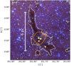 |
Fig. 1 The IRAC color composite image of the G351.77-0.53 filamentary region, where the 8.0 μm, 5.6 μm, and 3.6 μm are shown in red, green, and blue, respectively. The orange contour shows the coverage of the 3 mm data ALMA-IMF Large Program observations. The white contour represents the ATLASGAL emission (850 μm) at 0.62 Jy beam−1. The dominant central closed contour indicates the Mother Filament discussed below (also referred to as the “G351 filament” in Reyes-Reyes et al. 2024). This filament is also observed in NIR extinction and submillimeter emission. In its densest part, the star formation activity is revealed by strong NIR emission. |
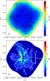 |
Fig. 2 Top: noise map of the fully combined N2H+ image (see text) in the G351.77 protocluster. The spectra with the highest noise values are located near the edges, as was expected. The mean rms value across the entire map is ~0.66 K, whereas the mean value in regions with S/N > 9 is ~0.40 K. Bottom: signal-to-noise ratio (S/N) map. Spectra with high S/N are distributed following filamentary structures. The contours show the areas where spectra with S/N ≥ 9 are found (see Appendix B). The ellipse in the bottom left corner represents the final beam size of the N2H+ data of 2.3″ × 2.1″, or 4.6 kau × 4.2 kau. |
2 Data
We analyzed the N2H+ (1–0) observations of the G351.77 protocluster in the 3 mm spectral band, observed by the 12 m-array, 7 m-array and TP configurations obtained from the ALMA-IMF Large Program (Motte et al. 2022). Our data has a maximum spatial resolution of ~4000 au and a spectral resolution of 0.23 km s−1. The beam sizes are (2.3″ × 2.1″), (16.9″ × 10.1″), and (69.6″ × 69.6″) for the 12 m-array, 7 m-array, and TP, respectively.
2.1 N2H+ data imaging
The data imaging process was performed using CASA 6.2 (CASA Team 2022) along with the ALMA-IMF data pipeline2. Initially, we imaged the 12 m-array data to determine the optimal parameter settings to achieve the highest quality results. Among the different parameters tested within the “tclean”3 CASA task, we explored different imaging results by varying: threshold, deconvolver, pbmask, pblimit and scales. These parameter values4 were selected based on the analysis of the residuals, model, and the image returned after each imaging process, in a way that minimized the residuals in the final product. Subsequently, we applied the same parameter values to combine the 12 m-array and 7 m-array data with “tclean” to increase the Fourier coverage (7M12M, henceforth). This combination produces artifacts such as peaks and bowls of intensity around the edges. These appear to be due to the differing UV-plane coverage of the 12 m-array versus 7 m-array, as well as the low signal near the edges. However, by increasing the pblimit value from 0.05 to 0.2 for this product – the later of which is a commonly used threshold in similar ALMA datasets – these artifacts are no longer produced, as the edge regions with lower sensitivity are effectively excluded.
Continuum subtraction was accomplished using the CASA task “imcontsub”. This task uses the channels free of line emission to generate a continuum model, which is subtracted from the line emission channels. This process yields the continuumsubtracted 7M12M data.
As a final step, we employed the CASA task “feather” to combine the 7M12M continuum subtracted data with the TP data to recover the extended line emission. Here we define the 7M12M continuum subtracted data as the high resolution data, and the TP as the low resolution data. Finally, we obtain a fully combined spectral cube (data cube, see Fig. A.1), with a spectral resolution of 0.23 km s−1, and whose size final synthesized beam is 2.3″ × 2.1″ and a Beam-Position-Angle (BPA) of 89°. The noise and signal-to-noise ratio (S/N) map of our imaged data are shown in Fig. 2. The mean root mean square (rms) value across the entire map is ~0.66 K, whereas the mean value in regions with S/N > 9 is ~0.40 K.
2.2 Other ALMA-IMF data
In our analysis, we used the smoothed “getsf” (Men’shchikov 2021) core catalog from Louvet et al. (2024), derived from the continuum images of the 1.3 mm band (Ginsburg et al. 2022a). We also utilized the core kinematics, integrated intensity map, and mean velocity map obtained from the DCN (3–2) spectral line fits from the 12 m-array (Cunningham et al. 2023). Further, we made use of the integrated intensity map and mean velocity map of H2CO (3–2) derived from the 12 m-array observations as part of the spectral setup of the ALMA-IMF Large Program (Motte et al. 2022). Additionally, we used an intermediate product of the H2 column density map of G351.77 at 6″ resolution, derived from a combination of 1.3 mm band, SOFIA/HAWC+ (53 μm, 89 μm, and 214 μm), APEX/SABOCA (350 μm) and APEX/LABOCA (870 μm) observations (Dell’Ova et al. 2024). Although the resolution of the final product of the H2 column density is 2.5″, we used this intermediate product in order to reduce the uncertainties of our estimations that could be produced by the combination of the data of H2 and from our fits. Moreover, this approach ensures a more uniform and reliable analysis by minimizing artifacts that may appear in maps at higher resolution and allows the calculation of one representative value of the relative abundance for the protocluster (Dell’Ova, private communication 2024).
3 Line fitting procedure
Since our main goal in this paper is to analyze the fine and large scale protocluster kinematics of dense gas, we require the use of spectral line fitting to retrieve the radial velocity field. Moreover, the line fitting of N2H+ (1–0) hyperfine structure provides additional parameters of interest; that is, the optical depth (τ) and excitation temperatures (Tex, see below). The first examination of the data cube immediately reveals that multiple velocity components exist over a significant number of spectra, consistent with previous research (e.g. Leurini et al. 2019, see Fig. 3). Hence, we adopted an iterative approach to line fitting, as is described in detail below.
We only fit spectra with S/N > 9. This approach stems from our experimental findings, which reveal that spectra with a S/N < 9 are inadequately fit, yielding high uncertainties in the returned parameters (see Fig. 2 and Appendix B). We ultimately fit the spectral cube with two velocity components when possible (driven mainly by S/N considerations, see Sect. 3.2) and one velocity component when the spectra are either relatively simple or the noise precludes more detailed velocity decomposition. To accomplish this fitting, we began with a one-velocity-component fit (see Fig. 4) and then with the two-velocity-components fit (see Fig. 4), which are independent. We refer to these two relatively “raw” fits as the first fitting procedures (FFPs). We then analyzed the S/N of the decomposed spectra to identify where we had reliable two-velocity-components fits; where we did not, we adopted the one-velocity-component fit for the spectrum being analyzed (see Sect. 3.3 and Fig. 5).
Here we use the N2H+ (1–0) line model “n2hp_vtau”5 from PySpecKit6 (Ginsburg & Mirocha 2011; Ginsburg et al. 2022b) to fit the cube (e.g., Redaelli et al. 2019; González Lobos & Stutz 2019; Álvarez-Gutiérrez et al. 2021). This model is a Local Thermodynamic Equilibrium (LTE) model, whose spectroscopic predictions come from known molecular data under the LTE assumption, such as rest frequencies and hyperfine structures. This procedure returns four parameters per velocity component: excitation temperature (Tex, see Fig. C.1), optical depth (τ, see Fig. C.2), centroid velocity (VLSR), and line width (σv), each representing a measurement for the entire spectrum.
To fit the data cube, four different guesses must be entered to initialize PySpecKit. In addition to the guesses, each parameter is assigned both a lower and upper limit value, defining the range within which the final fit values will lie. In Table 1, we show the guess and limit values for each parameter used in the FFP and in the final fit. After the fitting process, PySpecKit returns the model spectra, parameter values (see above), and associated parameter errors. Finally, applying methods in order to define the best fit for each spectra we merge the one and two velocity component fits into one model cube (see Sect. 3.3, Figs. 6, and 7 for example maps of the spectral fits, including the integrated intensity, mean velocity and the line width, and also Figs. C.1 and C.2 for examples of excitation temperature maps and optical depth maps). In the analysis in Sect. 3.4, we define the two main velocity components of the protocluster (see Figs. 6 and 7), where we also perform a careful measurement of the VLSR of G351.77 where <VLSR> = −3.843 ± 0.001 km s−1. In the text that follows, we present more details of the procedures outlined above, and we show in Sect. 3.4 that there is a continuity between the one and two velocity component fits except in some locations presenting jumps.
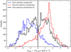 |
Fig. 3 Centroid velocity distributions of the one- and two-velocity-components fits. The black histogram represents the centroid velocity distribution of the spectra fit by the one-velocity-component model. The blue and red histograms show the centroid velocity distributions of the spectra fit with the two-velocity-components model, where blue corresponds to the first velocity component and red to the second velocity component. The solid black line represents the middle point X located at 0.025 km s−1, measured via Eq. (1) (see text). This divides the black histogram into two velocities, as explained in Sect. 3.4. |
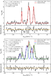 |
Fig. 4 Example of one-velocity (top) and two-velocity (bottom) component fits to two different spectra; the former (later) corresponds to a spectrum extracted from the blue (orange) areas in Fig. 5. In both panels: the data are represented on the top (solid black histograms) with their corresponding fits (colored curves), and the residuals are shown on the bottom, here the orange line refers to the nil value. The S/N of each spectrum, as well as the best-fit parameter values, are listed in each panel. In the bottom panel, the red curve represents the sum over the two velocity components. |
3.1 One-velocity-component fit
As an initial step, we employed a straightforward approach by fitting one velocity component across the entire spectral cube (see Fig. 4), entering the “FFP guesses” and “Limits” listed in Table 1. Since our goal is to achieve the best possible fit, we utilize the average of the parameters returned throughout the cube from the FFP to refine the input guesses, which are then applied in a new fitting process. New guesses are then estimated from these new fitting process. This is repeated until no variations are observed in the averages obtained for each parameter compared to previous fits. We define these parameter averages as “final guesses” (see Table 1). In this way, we provide PySpecKit values that are more representative of the data in order to produce the final model with a one-velocity-component fit.
The FFP reveals an issue produced by spectra with τ<1, which generates misleading estimations of Tex, whose values lie between 80 K ≲ Tex < 104 K. This issue also occurs in the two-velocity-components fitting. This problem arises due to the intrinsic degeneracy when fitting a single transition, which makes it impossible to measure both Tex and τ from the same transition when τ < 1. Since we aimed to preserve most of the data and use reliable values for each parameter, we address this issue by refitting the spectra with τ<1 and assigning them a constant Tex value (e.g., Caselli et al. 2002b,c).
Thus, spectra with τ<1 are selected and separated from the cube to be refit by a one-velocity-component with a constant Tex value, whose value comes from averaging Tex from spectra with τ > 1. The refit spectra use the final guesses listed in Table 1. However, the Tex limits are now 2.73 K to 12.4 K. At the end of this process, we obtain two separate spectral models and parameters from the spectra with τ ≥ 1, and from the spectra with τ<1 for the one-velocity-component fit, which correspond to the 64% and 36% of the spectra, respectively. As a final step in the fitting process, we merge these two spectral models and parameters, creating a final spectral model entirely fit by the one-velocity-component, with its corresponding parameters and associated errors.
Although this does not occur in every case, some spectra with τ ≫ 1 (τ ≳ 40) exhibit a “flat-top” effect at the intensity peak of the hyperfine structures in the model spectra. These spectra have errors in τ exceeding 100% and are excluded from the analysis. However, this occurs in less than 1% of the spectra, where the median value of τ ~ 3. The same issue arises in the two-velocity-components fits with similar frequency.
Guess and limit values entered for one- and two-velocity-components fits.
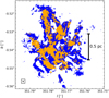 |
Fig. 5 Map of the number of velocity components in the N2H+ (1–0) spectral fits in the G351.77 protocluster. The blue (orange) pixels represent 59% (41%) of the spectra where we adopt a one-velocity-component fit (two-velocity-components fit), see Sect. 3.3. Most of the orange pixels are located in central regions, where we observe the highest S/N and integrated intensity values, similar to the results for G353.41 (Álvarez-Gutiérrez et al. 2024). The blue areas are located preferentially near the edges. The ellipse in the bottom left corner represents the beam size of the N2H+ data. |
3.2 Two-velocity-components fit
Upon examining the spectral cube, we notice the presence of two distinct velocity components in several spectra. Consequently, a one-velocity-component fit is not sufficient to describe the global kinematics of the data. This forces us to fit two velocity components in the spectral cube (see Fig. 4), entering the “FFP guesses” and “Limits” for each velocity component, listed in Table 1. In a similar way as we made in Sect. 3.1, and in order to get the best fit, we derive new guesses measuring the average of the values returned for each parameter of each component throughout the cube, until we obtain the final guesses (see Table 1), which are used to generate the final model with a two-velocity-components fit.
As we mentioned in Sect. 3.1, spectra with τ<1 produce bad estimations of the Tex. Therefore, spectra with τ<1 are selected and separated to be refit. However, because we are fitting two velocity components, it is necessary to separate the spectra into three different conditions (see Table 2) to assign them a constant Tex value. These constant values come from averaging Tex of spectra with τ ≥ 1 of each component. The refit spectra will use the same final guesses listed in Table 1, while the Tex limits depend on the opacity values (see Table 2).
The refitting process produces new τ estimations for spectra with τ ≈ 1 where the value can drop below 1. Specifically, this occurs in 5% of the total spectra when applying conditions 1 and 2 (see Table 2). As we already mentioned, these τ values generate bad estimations of Tex. It is necessary to select and separate the refit model spectra under two new conditions:
Model returned from the condition number 1 with τ2 < 1.
Model returned from the condition number 2 with τ1 < 1.
These spectra are refit again, using the final guesses and “Limits” of the Table 1. However, the Tex limits are now Tex = (2.73 K, 9.22 K) for the condition “a” and Tex = (2.73 K, 9.0 K) for the condition “b”. The separation of the cube into different conditions to refit the spectra with τ<1 provides us with the security that all spectra have greater freedom in order to estimate τ values and obtain good or more reliable Tex values in each spectrum.
At the end of this process, we obtain six separate model spectra and parameter cubes fit by two velocity components. One of these correspond to the model spectra with τ≥1, which account for 38% of the total spectra. The remaining five models spectra are derived from refitting process: conditions 1, 2, and 3 (see Table 2) represent 30%, 15%, and 11% of the final spectra, respectively, while the condition “a” and “b” (see above) contribute 3% and 2% to the final spectra, respectively. As a final step in this process, we merge these six spectral models and parameter cubes, creating a final spectral model entirely fit by two velocity components (see Fig. 6). We refer to each component as the “first velocity component” and the “second velocity component,” with their centroid velocities being the lowest and highest, respectively, and with their parameters and associated errors (see Fig. 4).
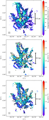 |
Fig. 6 Top: integrated intensity map from the final spectral model composed of both the one and two velocity components. Middle: line width map of the blue velocity component. Bottom: line width map of the red velocity component. The spectra inside the black contour are fit with two velocity components. The ellipse in the bottom left corner represents the beam size of the N2H+ data. |
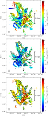 |
Fig. 7 Top: mean velocity map from the final spectral model composed of both the one and two velocity components. The red arrow display the direction of the Mother Filament. The blue arrow indicates the direction of the large-scale velocity gradient measured from the centroid velocities. Middle: centroid velocity map of the blue velocity component. Bottom: centroid velocity map of the red velocity component. The spectra inside the black contour are fit with two velocity components. The ellipse in the bottom left corner represents the beam size of the N2H+ data. |
Conditions and Tex limits for the refit of two velocity components.
3.3 Best fit and merging models
In Sects. 3.1 and 3.2, we described the complete fitting process of the data, fitting the whole cube with one and two velocity components. However, our spectral cube shows spectra where we can identify just one velocity component (see Fig. 4), spectra where we can identify two velocity components (see Fig. 4), and spectra where it is not possible to make a clear identification by eye. Furthermore, it is necessary to determine which fit (one or two velocity components) is better for each spectra to simplify our analysis and to recover reliable kinematic information about the protocluster. Thus, we devised a method to determine if one or two velocity components is appropriate for each spectrum based on S/N criteria and the parameters associated with each spectrum, specifically the line width.
In order to determine if the spectrum is better fit by one or two velocity components we:
Check the σv value in the spectral model fit by two velocity components. From inspection of the spectral model fit by two velocity components, we find some “false component” spectra without emission whose σv is equal to 0 km s−1 (see Fig. D.1). This implies that all spectra with these characteristics are better characterized by one-velocity-component fit (see Fig. D.1).
Measure the S/N of the velocity component with the lower intensity in the two-velocity-components fit. Deeper inspection shows that some additional velocity components have intensities similar to noise values. So, if the peak intensity is lower than five times the noise measured in that spectrum from the data cube, the one-velocity-component fit is adopted. Thus, we ensure the reliability of the additional velocity component (see Fig. D.2).
Additionally, all fit spectra with errors higher than five times the median error estimated for the centroid velocity (~0.2 km s−1) are removed for the kinematic analysis (see Sect. 5). For the estimation of column density (see Sect. 4), spectra with errors exceeding 10% for the line width, 30% for Tex, and 30% for τ are also excluded. These thresholds were estimated considering twice the median error measured for each parameter. Furthermore, we find that 95% of the spectra have error within the following ranges: [0.05 K, 1.78 K] for Tex, [0.4, 9.7] for τ, [0.007 km s−1, 0.26 km s−1] for the centroid velocity, and [0.1 km s−1, 0.17 km s−1] for the line width.
After applying these criteria, we obtain spectra well fit by one and two velocity components (see Fig. 4). All these spectra are merged in order to create a final spectral model composed of both one and two velocity components (see Fig. 5). Most of the spectra fit by two velocity components are located in internal regions toward highest integrated intensities (see Fig. 6).
3.4 Blue and red velocity components
From the four parameters returned by PySpecKit of the N2H+ (1–0) spectra, the centroid velocity is the one that has the lowest uncertainties with median values of 0.034 km s−1 (cases with higher errors than five times the median value are excluded, see Sect. 3.3), which gives us information about the radial velocity distributions of the regions where we observe line emission. The general centroid velocity distributions that we derive are plotted in Fig. 3, which we discuss in detail below.
The mean velocity map from the model in the top panel of Fig. 7, shows various interesting features. One of these includes indications of a large-scale velocity gradient (VG) that is almost perpendicular (~83°) to the direction in which the molecular cloud filament that hosts the protocluster extends (which we call the “Mother Filament,” see Fig. 1).
On the other hand, we observe jumps between the velocities of the spectra with one and two velocity components that reaches velocities of up to ~4 km s−1 (see top panel of Fig. 7). This is an effect produced by averaging the two centroid velocities in spectra with two velocity components, so is an artificial velocity averaging effect rooted in the complex motions in G351.77. Indeed, in the bottom two panels of Fig. 7, we separate the measured velocities and assign them to either a blue or red velocity component. To make this somewhat arbitrary but necessary velocity separation, we define the cut-off velocity as the midpoint based on the velocity distributions of the first velocity component and the second velocity component (see Fig. 3). We achieve this by applying the following simple relation:
![$\[<\mathrm{V}_{\mathrm{LSR}, 1}>+X \times \sigma_{\mathrm{v}_{\mathrm{LSR}, 1}}=<\mathrm{V}_{\mathrm{LSR}, 2}>-X \times \sigma_{\mathrm{v}_{\mathrm{LSR}, 2}},\]$](/articles/aa/full_html/2025/04/aa52589-24/aa52589-24-eq2.png) (1)
(1)
where < VLSR,1 > and < VLSR,2 > are the averaged centroid velocities of the first and second velocity component, respectively, σvLSR,1 and σvLSR,2 are the standard deviations of the centroid velocities in the first and second velocity component, respectively, and X represents the cut-off value used as the middle point, normalized by the standard deviations of the centroid velocity distributions.
Applying Eq. (1), we obtain X = 0.025. This value allows us to separate the centroid velocity distribution of the one-velocity-component fit into two parts and combine the measurements with the first and the second velocity component. We define the “blue velocity component” as the merger of all the spectra from the first velocity component and the spectra from the one-velocity-component fit with centroid velocity <0.025 km s−1, see middle panel of Fig. 7. Similarly, the “red velocity component” is the merger of all the spectra from the second velocity component and the spectra from the one-velocity-component fit with centroid velocity >0.025 km s−1 (see bottom panel of Fig. 7).
4 Column density, mass, and N2H+ relative abundance
The spectral line fitting of N2H+ (1–0) shown in Sect. 3 provides relevant information about the N2H+ (1–0) spectra, specifically excitation temperature (Tex), optical depth (τ), and line width (σv). These parameters enable the estimation of column density maps of N2H+, N(N2H+), calculated by Eq. (2) (see Fig. 8), and the mass of N2H+ in the protocluster, M(N2H+), calculated by Eq. (3), which can be determined for both the blue and the red velocity component (see Sect. 4.1). Additionally, the column density map of H2, N(H2), provided by Dell’Ova et al. (2024), shown in Fig. 9, gives us the opportunity to estimate the N2H+ relative abundances, X(N2H+), in the protocluster (see Fig. 10) covering ten out of eighteen 1.3 mm dust continuum cores (hereafter referred to as “dense cores”) from the core catalog of Louvet et al. (2024), see Table 3.
4.1 N2H+ column density and mass
In order to estimate the column density of N2H+, and given that Tex is not well constrained due to the low optical depth of some spectrum, we use the optically thick transitions approximation given by the following expression (Caselli et al. 2002c; Redaelli et al. 2019:
![$\[\mathrm{N}\left(\mathrm{~N}_2 \mathrm{H}^{+}\right)=\frac{4 \pi^{3 / 2}}{\sqrt{\ln (2)}} \frac{\nu^3 \cdot Q \cdot \sigma_v}{c^3 \cdot A_{u l} \cdot g_u} \frac{\tau}{e^{h \nu / k_b T_{e x}}-1} \cdot e^{E_u / k_b T_{e x}},\]$](/articles/aa/full_html/2025/04/aa52589-24/aa52589-24-eq3.png) (2)
(2)
where σv, τ, and Tex correspond to the parameters returned by our fits, while ν is the frequency, Q is the partition function, c is the speed of light, Aul is the Einstein coefficient, gu is the statistical weight, h is the Planck’s constant, kB is the Boltzmann’s constant, and Eu is the energy of the upper limit (Pagani et al. 2008; Mangum & Shirley 2017; Redaelli et al. 2019). The error of N(N2H+) is estimated making the error propagation over the Eq. (2). We apply this expression over the blue and the red velocity component to obtain the column density of each one, NB(N2H+) and NR(N2H+), respectively. The total column density NT(N2H+) is obtained by summing these (see Fig. 8 and Table 4). Then, we can measure the mass per pixel of N2H+ by applying the following expression:
![$\[\mathrm{M}\left(\mathrm{N}_2 \mathrm{H}^{+}\right)=\mathrm{N}(\mathrm{N}_2 \mathrm{H}^{+}) \cdot \mathrm{A}_{\text {pixel}} \cdot m_{\mathrm{N}_2 \mathrm{H}^{+}},\]$](/articles/aa/full_html/2025/04/aa52589-24/aa52589-24-eq4.png) (3)
(3)
where N(N2H+) is given by the Eq. (2), Apixel corresponds to the area of the pixel, and mN2H+ corresponds to the mass of N2H+ molecule, where mN2H+ = 4.817 × 10⁻²³ g. Table 4 shows the mass for the blue and the red velocity components as well as the total N2H+ mass in the protocluster.
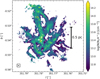 |
Fig. 8 N2H+ total column density map derived from Eq. (2). The ellipse in the bottom left corner represents the beam size of the N2H+ data. |
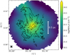 |
Fig. 9 H2 column density map from Dell’Ova et al. (2024) of the G351.77 protocluster. The black contour represents the spectra with NT(N2H+) > 1 × 1013 cm−2. The circle on the bottom left represents the beam size of 6″ × 6″. |
4.2 N2H+ relative abundance
We expect to estimate a new column density map of H2 (Ntot) and mass map of H2(Mtot) for both small and large scale structures (see Sect. 5), with at smaller spatial scale (see below) than the N(H2) provided by Dell’Ova et al. (2024). This estimation cannot be made with the ALMA-IMF dust emission given its small spatial coverage. However, the N2H+ emission provides us with a better angular resolution and a larger spatial coverage. For this is necessary to know the X(N2H+)in the protocluster, which is given by the following expression:
![$\[\mathrm{X}(\mathrm{N}_2 \mathrm{H}^{+})=\frac{\mathrm{N}(\mathrm{N}_2 \mathrm{H}^{+})}{\mathrm{N}(\mathrm{H}_2)},\]$](/articles/aa/full_html/2025/04/aa52589-24/aa52589-24-eq5.png) (4)
(4)
where the error of the relative abundance is estimated making the error propagation of the Eq. (4) utilizing the error maps of N(N2H+) and N(H2) at the same resolution.
Given the lower resolution of the N(H2) data (see Fig. 9), we performed a new fitting process of the N2H+ cube starting from the original spectral cube. In the first step, we convolved to a matched resolution and pixel scales the N(H2) data. Subsequently, we implemented the fitting processes shown in Sect. 3. In this way, it is feasible to analyze both datasets together in order to estimate the X(N2H+)correctly.
To ensure a more robust measurement of X(N2H+), we restricted our analysis to N(N2H+) and N(H2) regions with S/N in column densities >4. Applying Eq. (4), we obtained the relative abundance values for each pixel, which appears to follow a log-normal distribution (see Fig. 10). Based on these findings, our objective is to determine a representative value of X(N2H+), whose value will be equal to the mode of this distribution (the mean within the largest bin of the histogram, see Fig. 10). This allows us to compare structures across the whole protocluster and between the velocity components.
However, taking into account the significant scatter of X(N2H+), with values that ranging from ~10−11 to ~10−9, and considering that the mode may vary depending on the bin width used, we implemented the “Freedman Diaconis Estimator” method in order to derive the most representative value for the protocluster. This method7 provides the optimal bin width for a histogram, dividing the data sample into interquartile ranges, in order to equilibrate the distribution type, dispersion, and the size of the data sample.
Applying this method, the estimated optimal number of bins for our data distribution is 119 (see Fig. 10). With this number of bins, the mean within the largest bin (mode) corresponds to X(N2H+) = (1.66 ± 0.46) × 10−10. Additionally, by increasing the number of bins while preserving the log-normal shape of the distribution and averaging all the measured modes, we found that the modes converge to X(N2H+) = 1.66 × 10⁻¹⁰. Thus, we defined the representative relative abundance of G351.77 in the protocluster zone as X(N2H+) = (1.66 ± 0.46) × 10−10, whose value is within the ranges and magnitude order previously reported (e.g. Caselli et al. 2002a; Fontani et al. 2006; Henshaw et al. 2014). We used this value to determine Ntot and the Mtot at a higher resolution based on the N(N2H+) emission at its original resolution (before convolving it). This facilitates the measurement of the Mtot at smaller scales, allowing one to estimate masses related to dense cores and velocity gradients (see Table 5 and Sect. 5).
We estimate a total mass Mtot in the G351.77 protocluster of ~1660 ± 326 M⊙, which we consider a lower limit, since it corresponds to the mass derived only from the regions with N2H+ emission. Additionally, the total mass estimated directly from the dust-based H2 column density map from Dell’Ova et al. (2024) is M(H2) ~2820 M⊙. However, if we consider the mass inside the N2H+ coverage (at S/N > 9), we estimate a M(H2) ~2000 M⊙. This mass is within our uncertainties, and hence represents a good agreement considering the different tracers and techniques involved in this comparison. Given that the N(H2) map from Dell’Ova et al. (2024) is not affected by the interferometric filtering, like the N2H+ data of this research, the column densities, and then the masses, are correctly comparable. Our Mtot estimation is also consistent with the total mass measured in Reyes-Reyes et al. (2024), which represents ~16% of the total mass measured in the Mother Filament ~10 200 M⊙ in Reyes-Reyes et al. (2024). Aside from the global protocluster properties, we provide column densities, masses, and N2H+ relative abundances, in addition to the spectral fitting parameters (see Sect. 3 and Table 3) of the dense cores.
Physical parameters of the dense cores in G351.77 protocluster.
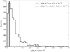 |
Fig. 10 Relative abundance X(N2H+) distribution in the G351.77 protocluster zone. The dashed red line represents the mean of the distribution. The dashed black line represents the mean inside the most prominent bin of the distribution. The shaded region represents the estimated error around the mode. |
Column densities and masses of N2H+ in G351.77 protocluster.
Total column densities and masses in G351.77 protocluster.
5 Kinematic analysis
The main goal is to analyze the kinematics of the dense gas within the G351.77 protocluster traced by N2H+ (1–0). The spectral line fitting process described in Sect. 3 provides us with the most reliable parameter measurable from each spectrum, the centroid velocity, whose median error estimations are ~0.034 km s−1. This centroid velocity, combined with the angular resolution of our data, enables us to analyze the kinematics of the protocluster on different scales (see below). To achieve this, we utilize PV diagrams (see Fig. 11), which correspond to projections of position-position-velocity (PPV) diagrams. These PV diagrams allow us to characterize PV features, which may be produced by inflow, rotation, outflow, or cloud-cloud collisions (Tobin et al. 2012; Henshaw et al. 2014; Haworth et al. 2015; Mori et al. 2024), and access to the physical information occurring at both approximately small and large scales. To simplify the analysis, we therefore defined small scales as scales from the resolution limit of the observations, or the “dense core” scales, of about 4 kau to about ten times larger. Conversely, larger scales encompass approximately from filament scales to the protocluster scale, so ~ 0.2 pc to 1.2 pc.
In addition, we created and analyzed PPV diagrams8, in order to inspect and distinguish PPV structures. This way, it was possible to extract structures at both small and large, potentially coarser, scales. In doing so, we isolated structures based on PPV distributions combined with their integrated intensity. We then analyzed these while avoiding degeneracies that might arise from the use of projected PV diagrams alone.
We utilized three parameters to generate the intensity-weighted PV diagrams shown in e.g., Fig. 11. These parameters are the centroid velocity, integrated intensity (excluding points with emission below 11 K km s−1 to avoid introducing noise and to better highlight the dominant structures in the diagrams), and b or l coordinates (e.g. Henshaw et al. 2014; González Lobos & Stutz 2019; Álvarez-Gutiérrez et al. 2021; Redaelli et al. 2022; Álvarez-Gutiérrez et al. 2024). The top left panel of Fig. 11 shows the spatial distribution of the N2H+ (1–0) emission, where the blue and red color bars represent the blue and red velocity components described in Sect. 3.4. The top right and bottom left panels display PV diagrams, where the color of each point represents the integrated intensity weighted.
5.1 Kinematic analysis on small scales
A cursory inspection of Fig. 11 reveals distinct PV features along the filamentary structures present in both the blue and the red velocity components, some of which appear to be consistent in position both with the dense cores (Louvet et al. 2024) and with their estimated DCN (3–2) velocities (see Table F.9 in Cunningham et al. 2023).
We analyzed the N2H+ (1–0) velocities around the dense cores within a radius six times the size of the dense core (~ 0.1 pc, see Table E.11 Louvet et al. 2024). This radius criteria enables us to examine the behavior of the surrounding gas while avoiding the overlap of gas around other cataloged dense cores. Subsequently, we recreated the PV diagrams of N2H+ (1–0) emission in the vicinity of the dense cores, which permitted the identification of two distinct types of features:
V-shapes: where the dense core is positioned at or near the point where we measure the inflection point in the velocity field of N2H+ (1–0), and the surrounding gas transitions toward lower or higher velocities (see Fig. 12 and Álvarez-Gutiérrez et al. 2024).
Straight shapes: where the gas around the dense core transitions from high to low velocities, while the dense core is located ~ halfway along this straight shape (see Fig. 13; see also Fig. 1 in Tobin et al. 2012).
From the 1.3 mm continuum data, 18 dense cores have been cataloged (see Table E.11 in Louvet et al. 2024), of which 9 are located in zones with N2H+ (1–0) integrated intensity higher than 11 K km s−1 and S/N > 9 (see Fig. 11). However, only six dense cores have identifiable kinematic patterns in the PV diagram (three V-shapes and three straight shapes, see Table E.1).
In order to characterize the V- and straight shapes, we applied a linear fit to the observed VGs, encompassing the upper and lower VG for the V-shapes (see Figs. 12 and 13). The selection criteria for the points used in the fit were based on their integrated intensity and location along the V-shape structure. This approach allowed us to specifically characterize the enveloping points of the V-shape structure, effectively providing a boundary or limit for the measurements derived from the characterization. For the linear fitting process, the integrated intensity was used as a statistical weight. After characterizing the VGs, we estimated their associated timescales as ![$\[t_{\mathrm{VG}}=\frac{1}{\mathrm{VG}}\]$](/articles/aa/full_html/2025/04/aa52589-24/aa52589-24-eq6.png) (e.g., Álvarez-Gutiérrez et al. 2021, 2024). Furthermore, we measured the Mtot (Sect. 4) associated with the points used to quantify the VGs in order to estimate the mass inflow rate
(e.g., Álvarez-Gutiérrez et al. 2021, 2024). Furthermore, we measured the Mtot (Sect. 4) associated with the points used to quantify the VGs in order to estimate the mass inflow rate ![$\[\dot{\mathrm{M}}_{\text {tot,in}}\]$](/articles/aa/full_html/2025/04/aa52589-24/aa52589-24-eq7.png) following:
following:
![$\[\dot{\mathrm{M}}_{\mathrm{tot}, \text { in }}=\frac{\mathrm{M}_{\mathrm{tot}}}{t_{\mathrm{VG}}}.\]$](/articles/aa/full_html/2025/04/aa52589-24/aa52589-24-eq8.png) (5)
(5)
We note that the above analysis of the VG and timescales is affected by the inclination angle, θ, of the filament relative to the plane of the sky. The relationship is given by tVG = l/vr tan (θ), where l represents the projected length of the filament in the plane of the sky, vr denotes the radial velocity, and θ is the inclination angle of the filament. For our purposes, we cannot measure the inclination of any given structure. The assumptions here are equivalent to assuming a 45° average inclination angle for all timescales and ![$\[\dot{\mathrm{M}}_{\text {tot,in}}\]$](/articles/aa/full_html/2025/04/aa52589-24/aa52589-24-eq9.png) . Besides, Álvarez-Gutiérrez et al. (2024) show in their Fig. 11 that the estimated gradients (which they measure in a similar fashion as here) do not depend on the orientation angle of the spatial axis used in the PV diagrams. That is, V-shapes extracted along the b coordinate still appear as clear V-shapes at other angles with gradients (and so timescales).
. Besides, Álvarez-Gutiérrez et al. (2024) show in their Fig. 11 that the estimated gradients (which they measure in a similar fashion as here) do not depend on the orientation angle of the spatial axis used in the PV diagrams. That is, V-shapes extracted along the b coordinate still appear as clear V-shapes at other angles with gradients (and so timescales).
Focusing on the most prominent V-shape, we identify two clear VGs associated with a dense core (L19 in Fig. 14 and Table E.1). This dense core is located in the region with the highest N2H+ (1–0) emission, where the spectra are fit by two velocity components. We measured the VGs, timescales, mass, and mass inflow rate of the six PV features associated with dense cores, and we present these parameters in Table E.1.
Henshaw et al. (2014) proposed two physical processes related to the V-shapes structures in PV diagrams: inflows and outflows. However, we do not observe an agreement between the position of outflow catalogs (e.g. Towner et al. 2024) and the position of dense cores associated with V-shapes in PV diagrams. We propose that the points utilized for the characterization of the VG in V-shapes represent the inflowing gas with the highest velocity along a filamentary structure, where the dense core may be located in a “knee” in the filament (see Fig. 12 and Álvarez-Gutiérrez et al. 2024 for similar interpretation of the V-shapes). On the other hand, the straight shapes may be explained as filamentary structures with embedded dense cores, where the filaments inflow toward the inner and denser regions and the dense cores follow the stream of the surrounding gas, flowing along with the filaments (Hacar & Tafalla 2011; Lu et al. 2018; Motte et al. 2018; Kim et al. 2022; Arzoumanian et al. 2023; Yang et al. 2023; Pan et al. 2024).
Continuing the PV analysis at scales of six times the average radius of the dense cores, some of these PV features are even found without any detected dense cores (see Fig. 14 and Table E.1).
Utilizing the PPV diagram, we find 16 PV features both V- and straight shapes in the protocluster without associated dense cores (see Fig. 14). We distinguish between these small scale PV features based on the velocity distribution in the PPV diagram and increases in integrated intensity. This way, we can rule out the possibility that a given PV feature is produced by the overlap of points that do not share nearby regions in the position-position diagram. We measured the VGs, timescales, mass, and ![$\[\dot{\mathrm{M}}_{\text {tot,in}}\]$](/articles/aa/full_html/2025/04/aa52589-24/aa52589-24-eq11.png) of the PV features (see Table E.1). Both the integrated intensities measured in the regions where these PV features are observed and the estimated
of the PV features (see Table E.1). Both the integrated intensities measured in the regions where these PV features are observed and the estimated ![$\[\dot{\mathrm{M}}_{\text {tot,in}}\]$](/articles/aa/full_html/2025/04/aa52589-24/aa52589-24-eq12.png) values appear similar to what we have estimated for the PV features associated with dense cores.
values appear similar to what we have estimated for the PV features associated with dense cores.
Furthermore, it is possible to observe some consistences in position-position between the cores candidates and the cores detected by “GExt2D” (Louvet et al. 2024). We suggest a relation between these PV features and possible cores that are under the detection limit on the 1.3 mm data (undetected by “getsf”) or regions where the gas is just beginning to accrete. We propose the location of these possible cores (see Table E.1) as the spatial locations of the vertexes of the V-shapes. Moreover, based on the dense cores and the associated PV features, we may expect a discrepancy of no more than ~0.03 pc between the proposed positions and the locations of the undetected cores. This because some gas flowing through filaments may move toward a local or global maximum of the gravitational potential, which might not necessarily coincide exactly with the position of a core (Izquierdo et al. 2018). Additionally, inflowing gas along filaments can be disturbed by turbulence, shear, interaction with molecular outflows, H II regions, and other dynamical processes (Guerrero-Gamboa & Vázquez-Semadeni 2020; Vázquez-Semadeni et al. 2024). These effects, in addition with projection effects, could explain the discrepancies observed between the position of dense cores and the vertex of the V-shapes, which, nevertheless, are always within about the beam size (see Fig. 12).
The estimation of ![$\[\dot{\mathrm{M}}_{\text {tot,in}}\]$](/articles/aa/full_html/2025/04/aa52589-24/aa52589-24-eq13.png) of these PV features, particularly the V-shapes, could be correlated with the dense core mass buildup, due to the convergence of VGs at some dense core positions (see Fig. 12 and Álvarez-Gutiérrez et al. 2024). Moreover, the estimated tVG could suggest the timescale for the collapse of filamentary structures toward dense cores (Álvarez-Gutiérrez et al. 2024). In total, we observe 17 V-shapes (see Table 6), where the average values of tVG = 43.73 ± 0.94 kyr and
of these PV features, particularly the V-shapes, could be correlated with the dense core mass buildup, due to the convergence of VGs at some dense core positions (see Fig. 12 and Álvarez-Gutiérrez et al. 2024). Moreover, the estimated tVG could suggest the timescale for the collapse of filamentary structures toward dense cores (Álvarez-Gutiérrez et al. 2024). In total, we observe 17 V-shapes (see Table 6), where the average values of tVG = 43.73 ± 0.94 kyr and ![$\[\dot{\mathrm{M}}_{\text {tot,in}}\]$](/articles/aa/full_html/2025/04/aa52589-24/aa52589-24-eq14.png) = 5.59 ± 0.34) × 10−4 M⊙ yr−1.
= 5.59 ± 0.34) × 10−4 M⊙ yr−1.
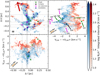 |
Fig. 11 Integrated intensity and PV diagrams of the blue (blue color bar) and red (red color bar) velocity components seen in N2H+ (1–0). Top left: spatial distribution of N2H+ (1–0) emission in G351.77. The green, black, and magenta × markers indicate the positions of the 9 out of the 18 (see Sect. 5.1) dense cores (Louvet et al. 2024), where each color represents the DCN spectral classification: single, complex, and non-detected, respectively (Cunningham et al. 2023). The + markers indicate the position of the 16 core candidates, proposed on the basis on the N2H+ PV features observed at scales of ~0.1 pc (see Sect. 5.1 and Table E.1). Dashed lines indicate the positions of the four dense cores that do not have measurable velocities. The red arrow indicates the direction of the Mother Filament. The ellipse in the bottom left represents the beam size of the N2H+ data. Top right and bottom left: PV diagrams along the two perpendicular directions. Top right: the colored arrows indicate the position of the dense cores and their ID in Table 3. We observe multiple structures, such as V-shapes and Straight structures (see text) along the filaments, some associated with dense cores in both position and velocity. The orange arrows represent a velocity gradient of 10 km s−1 pc−1 ≈ 0.1 Myr. |
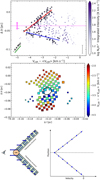 |
Fig. 12 Top: PV diagram of the most prominent V-shape (L19 in Fig. 11). The black outlined points show the points used in order to generate the linear fits of the velocity gradients. The red and blue lines represent the upper and lower VG, respectively, which converge at ~ 0.015 pc below the central position of the dense core. The magenta error bar represents the projected size of the dense core (Louvet et al. 2024), while the horizontal dashed line represents the position of the dense core. The color bar shows the integrated intensity of N2H+ (1–0) levels. The gray error bar represents the beam size of the N2H+ data. The green arrow represents a velocity gradient of 25 km s−1 pc−1, which corresponds to a timescale of ~0.4 Myr. Middle: Position-position diagram of the most prominent V-shape. The squares represent the points used for the linear fit (top figure). The size of the squares correspond to the integrated intensity of each spectrum, while the ellipse indicates the position and size of the dense core (L19 in Fig. 11). Bottom right: Proposed model for the observed PV features as V-shapes (see also Fig. 12 in Henshaw et al. 2014 and Álvarez-Gutiérrez et al. 2024). Bottom left: inflowing filamentary structure. The light blue and blue arrows represent the velocity magnitude of the gas and the radial component of the gas velocity, respectively. Right: PV diagram of the model. |
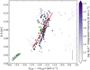 |
Fig. 13 PV diagram of a single core (L18 in Table E.1) from the catalog of Louvet et al. (2024). The PV feature outlines what we define as a straight shape. The black outlined points show the points used to generate the linear fit of the velocity gradient. The red line represents the linear fit of the velocity gradient. The green × marker indicates the position (Louvet et al. 2024) and velocity of the dense core measured in DCN (see Table F.9 in Cunningham et al. 2023), while the green bar indicates the projected dense core size. The gray error bar represents the beam size of the N2H+ data. The green arrow represents a velocity gradient of 25 km s−1 pc−1, which correspond to a timescale of ~0.4 Myr. |
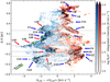 |
Fig. 14 PV diagram of the blue (blue color bar) and red (red color bar) velocity components seen in N2H+ (1–0). The dark points highlight the PV features observed. The blue arrows represent the location of the 16 PV features of candidates cores under the 1.3 mm band detection limit (see Table E.1). The red arrows indicate the location in the PV diagram of PV features associated with the dense cores (Louvet et al. 2024, see Table E.1). The markers and dashed lines are the same as in Fig. 11. The green arrow represents a velocity gradient of 10 km s−1 pc−1, which correspond to a timescale of 0.1 Myr. |
Averaged characterization of the N2H+ V-shapes observed PV diagram.
5.2 Kinematics analysis on large scales
The PV diagram of the N2H+ (1–0) emission, from filament scales to protocluster scales (~0.2 pc to ~1.2 pc) reveals two distinct large-scale structures, separated by ~2 km s−1 (see Fig. 11). One appears to be dominated by the blue velocity component, while the other is characterized by the red velocity component. Furthermore, these two velocity structures seem to merge or tighten up toward the Galactic northern region of the protocluster, in the direction toward the Mother Filament (see top left panel in Fig. 11). These large-scale structures present PV features like a zig-zag along the protocluster, which we suggest are produced by kinematic effects at smaller scales (see Sect. 5.1). However, upon deeper examination of the kinematics and inspection of the PPV diagram, we realize that these largescale structures are not only separated in velocity but also by spatial position (see Fig. 15).
In order to analyze these structures and identify the largescale regions contributing to the features observed in the PV-diagram, we divided the emission into four regions (F1, F2, F3, and F4) defining clear boundaries for each. This separation was guided by the integrated intensity map, SNR map, and the column density map, allowing us to distinguish between possible filamentary structures. The criteria used include integrated intensities drop below 50 K km s−1 (excluding F3) and velocity differences larger than ~0.9 km s−1, enabling us to separate structures that exhibit sharp velocity transitions (see Fig. 15):
F1: this corresponds to the primary filamentary structure within the protocluster, where we observe the highest S/Ns, integrated intensities, and column densities. It is connected with the three other large-scale structures (F2, F3, and F4) defined within the protocluster. Furthermore, six out of the nine dense cores, from Louvet et al. (2024), located in regions with N2H+ emission, are situated within this filamentary structure. Notably, this structure exhibits large-scale velocity distributions converging near the position of the dense core (L19 in Table 3) where we observe the most prominent V-shape (see Sect. 5.1) along with three straight shapes associated with dense cores. Furthermore, along this structure, we find some small-scale PV features that we suggest represent cores under the detection limit (see Sect. 5.1). Most of the spectra in this structure are characterized by two velocity components.
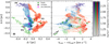
Fig. 15 Integrated intensity and PV diagram of the F1 (blue color bar), F2 (red color bar), F3 (green color bar), and F4 (purple color bar) largescale structures of N2H+ (1–0) into which the protocluster has been divided. Left: Spatial distribution of N2H+ (1–0) emission. Markers and dashed lines are the same as in Fig. 11. The ellipse in the bottom left represents the beam size of the N2H+ data. Right: PV diagram. We observe multiple large-scale V-shapes and straight shapes along the different filamentary structures, with some of them associated with dense cores in position and in velocity. The green arrows represent a velocity gradient of 10 km s−1 pc−1, which correspond to a timescale of ~0.1 Myr.
F2: adjacent to F1, the F2 structure is the next most obvious filamentary structure within G351.77. It connects to the F1 structure near the protocluster’s center through regions with low integrated intensity, but it merges with the F1 structure toward the Galactic north of the protocluster. This structure appears as a twisted filament, less monolithically well defined than F1 and not converging to a specific location. Nonetheless, two Louvet et al. (2024) dense cores are situated inside F2, as well as ~50% of the V- and straight shapes. Multiple spectra within this structure are characterized by two velocity components.
F3: located to the south of F1, F3 displays at least two clear velocity components along its length with a Δv reaching ~3 km s−1. F3 contains one dense core (L13 in Table 3), coinciding with the position where the filament exhibits a large-scale V-shape in the PV diagram (see Fig. 15). Two of the core candidates are located at the Galactic south of this structure.
F4: situated in the northern region of the protocluster, where F1 and F2 merge, the F4 structure presents well defined V- and straight shapes without associated cores. This region is connected with the Mother Filament.
As a whole, these structures do not appear drastically different from each other in terms of their internal kinematics; we observe PV features in all of them.
6 Discussion
6.1 G351.77 versus the G353.41 protocluster
In Sect. 5.1, we characterized the PV features associated with dense cores as well as PV features without cores, suggesting that the dense gas material traced by the N2H+ (1–0) line is inflowing in filamentary structures into dense cores or in larger scales inflowing toward denser regions (see also Hacar et al. 2017; Lu et al. 2018; Motte et al. 2018; Álvarez-Gutiérrez et al. 2021; Kim et al. 2022; Arzoumanian et al. 2023; Yang et al. 2023; Álvarez-Gutiérrez et al. 2024; Pan et al. 2024). The recent N2H+ analysis in the G353.41 protocluster (Álvarez-Gutiérrez et al. 2024), also observed by ALMA-IMF at matched physical resolution to the observations presented here, shows similar kinematic features although they use the N2H+ (1–0) isolated hyperfine component. The comparison to G351.41 is relevant beyond the similarities in the analysis techniques and the matched sensitivity and spatial resolution provided by ALMA-IMF.
Both protoclusters have similar masses, sizes, distances (Motte et al. 2022; Reyes-Reyes et al. 2024; Dell’Ova et al. 2024), and both exist inside isolated filamentary structures (see Fig. 1 and Álvarez-Gutiérrez et al. 2024).
Moreover, G351.77 and G353.41 have both been classified as existing in an intermediate evolutionary stage (Motte et al. 2022), based predominantly on H41α emission (see also Galván-Madrid et al. 2024). In finer detail, the larger number of dense cores and the smaller number of PV features in G353.41 compared to G351.77 together suggest that G351.77 is in a younger evolutionary stage relative to G353.41. Álvarez-Gutiérrez et al. (2024) characterized multiple V-shapes associated with dense cores, which they suggest are inflowing material onto or near dense cores, similar to our results. Almost all of the V-shapes in G353.41 are located inside filamentary structures; moreover, the tVG and ![$\[\dot{\mathrm{M}}_{\text {tot,in}}\]$](/articles/aa/full_html/2025/04/aa52589-24/aa52589-24-eq15.png) are similar (within the same order of magnitude) as those measured here for G351.77. This indicates that the V-shapes observed in PV diagrams represent generic kinematic features in forming protoclusters and can be used more broadly to access the conditions during the assembly of stellar clusters and the so called “initial conditions” of star formation, especially for the kinematic attributes.
are similar (within the same order of magnitude) as those measured here for G351.77. This indicates that the V-shapes observed in PV diagrams represent generic kinematic features in forming protoclusters and can be used more broadly to access the conditions during the assembly of stellar clusters and the so called “initial conditions” of star formation, especially for the kinematic attributes.
By averaging the VGs of the V-shapes associated only with the dense cores (see Table 6), we estimate a timescale ~32.96 ± 1.58 kyr. Conversely, by averaging the VGs of the V-shapes not associated with the dense cores, we estimate a timescales of ~43.12 ± 1.10 kyr. When averaging all the VGs associated with the V-shapes, we estimate a timescale of ~41.33 ± 0.95 kyr. We observe that the average timescale estimated in G353.41 protocluster is ~2× higher than the value measured in G351.77. This may also corroborate the above suggestion that G351.77 is younger, whereby the dense cores in the protocluster (which are also more numerous) may be accumulating mass faster than in G353.41, despite the mass reservoir similarity in both protoclusters (see above).
6.2 G351.77 on small scales
The longest timescale we measure for a V-shape is 69.17 ± 8.95 kyr (see Table 6), whose time is lower than the lifetime of the prestellar cores (Valeille-Manet et al. 2025). Although we have not observed protostellar cores within the G351.77 protocluster, we expect that these PV features will disappear before the dense cores enter the protostellar phase, unless these structures are continuously fed with gas in some way. This could suggest that more evolved regions should display fewer V-shapes features in dense gas, which would be more closely associated with dense cores rather than prestellar and protostellar cores.
Additionally, utilizing the mass and sizes of the dense cores from Table D.11 in Louvet et al. (2024), associated with the V-shapes, we measure the free-fall time (tf f) for each dense core, whose average is ~13.6 kyr. This value is ~2.5 times lower than the average timescale for the V-shapes (~33 kyr, see Sect. 6.1), and similar to the value measured in the G353.41 protocluster (see Álvarez-Gutiérrez et al. 2024), suggesting that the dense cores may collapse gravitationally before the V-shapes dissipate. The accumulation of mass into the dense cores via the V-shapes would increases the dense core densities, further reducing tf f and accelerating the gravitational collapse. Consequently, the dense cores could collapse on shorter timescales, limiting the time available for sustained gas accretion from the V-shapes. This implies a dual role for the V-shapes: directly feeding the dense cores while potentially generating new dense regions along the filaments produced by local accumulation of gas. Further, collateral effects from dense core collapse, such as outflows, feedback, and concentration of magnetic fields, could significantly influence the dynamics of these structures. In an evolutionary context, these interactions could affect dense core evolution, and the properties of the stars formed within. The increase in dense core mass could impact the initial mass function (IMF), and the core mass function (CMF) measured in the protocluster (see Louvet et al. 2024). These effects suggest that the relation between the V-shapes, the dense cores, and the larger filamentary structures regulates gas supply of gas, evolution timescales, and star formation efficiency in the protocluster.
Furthermore, we estimate the total mass accretion rate considering both the V-shape structures associated and not associated with the dense cores (see Table 6). The total mass accretion rate measured is ![$\[\dot{\mathrm{M}}_{\text {in,T}}\]$](/articles/aa/full_html/2025/04/aa52589-24/aa52589-24-eq16.png) = (9.84 ± 0.63) × 10−3 M⊙ yr−1. Considering the total mass of the protocluster is ~2820 M⊙, we can estimate the depletion timescales given by tdep = Mtot/
= (9.84 ± 0.63) × 10−3 M⊙ yr−1. Considering the total mass of the protocluster is ~2820 M⊙, we can estimate the depletion timescales given by tdep = Mtot/![$\[\dot{\mathrm{M}}_{\text {in,T}}\]$](/articles/aa/full_html/2025/04/aa52589-24/aa52589-24-eq17.png) , obtaining a tdep ~ 0.3 Myr.
, obtaining a tdep ~ 0.3 Myr.
A tdep ~ 0.3 Myr for the V-shapes is consistent with the short lifetime of dense gas traced by N2H+, as described in the simulations of Priestley et al. (2023), where N2H+ is exclusively associated with dense gas typically linked to material that will collapse to form stars. This suggests that the V-shapes associated with dense cores could represent gas in stages of gravitational collapse. In contrast, the V-shapes without associated dense cores could be material in transit toward higher densities, eventually becoming linked to star formation. Hence, we suggest that the V-shapes may serve as tracers of the early star formation rate (SFR) and the evolutionary stage of star-forming regions (see e.g., Dib et al. 2025, for the discussion on the efficacy of YSOs as SFR tracers).
Moreover, the fast tdep measured could represent not only an ongoing star formation in early stages, but also the need for continuous mass feeding from the larger scales, such as the Mother Filament (see below). This scenario maybe consistent with the finding of Hacar et al. (2024), where they identified dense fibers as structures moving material into forming star clusters. These fibers could continuously feed the protocluster, compensating the fast depletion of the local gas and enabling efficient star cluster formation. We caution that without direct confirmation of inflow onto a central mass (the dense cores in this case), the depletion timescales associated with the total sample of all V-shapes may be overestimated.
6.3 G351.77 on large scales
Moving to somewhat larger scales, in Sect. 5.2 we divided the N2H+ (1–0) emission of the G351.77 protocluster into 4 larger (~0.2 pc to ~1.2 pc) spatially distinguishable regions or filaments inside the protocluster. In particular, we show that the F1 filamentary structure seems to be inflowing toward a dense core, where we observe the most prominent V-shape in the PV diagram (see Figs. 11 and 15). Given that F1 filamentary structure is connected with the F4 structure, the region which is directly connected with the Mother Filament, and its velocity distribution observed in PPV diagrams, we suggest that the inflowing gas is coming from the Mother Filament, flowing toward the protocluster (e.g. Hacar et al. 2024). Furthermore, we find dense cores associated with straight shapes in the G351.77 protocluster, located along of the F1 filament structure (see Fig. 11), near the position where we observe the most prominent V-shape. Considering the velocity distribution of N2H+ displayed in the PV diagrams of straight shapes, their location, and the consistency of the N2H+ (1–0) velocities with those measured for the dense cores (see Table F.9 in Cunningham et al. 2023), we propose that these dense cores are inflowing, along with the N2H+, toward the location of the most prominent V-shape, potentially entrained in the slow contraction of the protocluster (Lu et al. 2018; Motte et al. 2018; Kim et al. 2022; Arzoumanian et al. 2023; Yang et al. 2023; Pan et al. 2024). All this, may suggests that the F1 structure is actively forming cores or stars.
In contrast to F1, the F2 filamentary structure does not show evidence of inflowing gas toward a specific location but rather presents inflow toward different locations along the structure. Moreover, most of the PV features on small scales do not have associated detected dense cores, which we propose as cores below the 1.3 mm band detection limit, located within the filament. This may suggest that this filamentary structure is participating in the formation of cores but at an earlier stage than the F1 structure. Additionally, hot cores are located in regions with N2H+ emission with S/N < 9, limiting the kinematic information available from them. Regarding the detected SiO outflows (see Towner et al. 2024), we identify four in F1 and two in F2, but none are associated with well-defined structures in the PV-diagrams. Instead, these outflows are located at the edges of the N2H+ emission rather than the internal regions of the filaments. This spatial distribution suggest that ongoing star formation activity may not be occurring within the densest regions of the filaments but rather in their outskirts. Furthermore, the more well-defined morphology of F1 compared to F2 supports the idea that these two exist at different evolutionary stages (see also Cunningham et al. (2023) for the proposal of multiple stages inside a given ALMA-IMF protocluster).
The F3 filamentary structure shows little evidence of star formation activity within it, where we find one dense core, and two PV features at small scales without associated dense cores. The PV features and the large-scale velocity distribution of this filamentary structure in PPV diagrams, seems to indicate that the gas in this is inflowing toward the dense core location.
The F4 structure presents velocity distributions in the PPV diagram (see Figs. 11 and 15) that supports the idea that the inflowing gas toward the denser N2H+ regions of the protocluster originate from the Mother Filament. Additionally, this region may also be a site where cores or stars could be forming, given the presence of PPV features on small scales that do not have detected dense cores associated.
6.4 G351.77 in a global hierarchical collapse scenario
The evidence that we have at small and large scales is consistent with the global hierarchical collapse (GHC) scenario described in Vázquez-Semadeni et al. (2019). This scenario explains the collapse process occurring on different scales in molecular clouds, where mass and gas flow and accrete through filamentary structures toward clumps and denser regions. It also describes how the timescales of accretion and contraction are shorter on smaller scales. These timescales play an important role in the SFR, with longer timescales allowing most of the mass to be dispersed due to feedback from massive stars, which later results in a low SFR.
Thus, by comparing the GHC model with our analysis, we suggest that the Mother Filament is undergoing global collapse, with a portion of it accreting and contracting toward the G351.77 protocluster. This implies that the protocluster will increase its mass over time. Although there is evidence of YSOs in the central part (Leurini et al. 2011a; Yu et al. 2018; Leurini et al. 2019; Sabatini et al. 2019), the H41α emission is compact in the central region of the protocluster (Motte et al. 2022; Galván-Madrid et al. 2024), where there is no N2H+ emission (S/N < 9). This suggests that currently there is insufficient feedback to significantly reduce the SFR in the protocluster (Vázquez-Semadeni et al. 2019). This indicates that the low SFR measured in G351.77 and along the Mother Filament (see Reyes-Reyes et al. 2024) may be due to the fact that the molecular cloud and the protocluster are still in a young stage, consistent with our suggestions and those in Reyes-Reyes et al. (2024). Consequently, the SFR is expected to increase with the formation of more massive stars until feedback from these new stars disperses the gas, thereby decreasing the SFR (Vázquez-Semadeni et al. 2019).
Given that we suggest the G351.77 protocluster is younger than G353.41, and based on the GHC model (Vázquez-Semadeni et al. 2019), we could anticipate a higher SFR in G353.41. This expectation aligns with the H41α emission in G353.41, which is higher than in G351.77 (see Table 4 in Motte et al. 2022), indicating a larger amount of massive star feedback in the G353.41 protocluster. However, a larger number of hot cores are observed in G351.77 compared to G353.41 (Bonfand et al. 2024), presenting a scenario that could contradict the notion of G351.77 being younger, as we might expect to find more hot cores in more evolved regions. Nevertheless, considering the various lines of evidence suggesting that G351.77 in indeed younger, we propose that some as of now unknown process may be inhibiting the formation of hot cores in G353.41 protocluster.
6.5 Multi-tracer modeling
In order to complement and enhance our understanding of the kinematic processes occurring in the protocluster at large scales, we utilize H2CO (2–1) and DCN (3–2) line emission covering the central part of the protocluster without N2H+ emission (Motte et al. 2022; Cunningham et al. 2023). Additionally, we modeled three possible cases for gas spheres: rotation-only, infall-only, and a combination between rotation and infall (see Appendix F), whose radial velocities are used to recreate PV diagrams (e.g., Tobin et al. 2012; Henshaw et al. 2014; Mori et al. 2024; Álvarez-Gutiérrez et al. 2024). This approach allows us to analyze the PV features produced by these kinematic processes in the PV diagrams (see Fig. 16)
The modeled sphere is formed by n numbers of points, which are under gravitational infall and keplerian rotation. The velocity associated with each point is estimated by using the following relations:
![$\[V_{\mathrm{in}}=-\sqrt{\frac{2 G M}{r}}, \quad V_{\mathrm{rot}}=\sqrt{\frac{G M}{r}},\]$](/articles/aa/full_html/2025/04/aa52589-24/aa52589-24-eq18.png) (6)
(6)
where r is the distance of each point to the center of the sphere, G is the gravitational constant, and M is the enclosed mass. The minimum distance between each point is of 0.007 pc, in order to simulate the pixel width of our data. Additionally, the sphere has a density profile that follows a power law described below:
![$\[\rho(r)=\rho_0\left(\frac{r}{\mathrm{pc}}\right)^{-\gamma},\]$](/articles/aa/full_html/2025/04/aa52589-24/aa52589-24-eq19.png) (7)
(7)
where r is the distance to the center of the sphere, and ρ0 is a known density. To generate an infalling and rotating sphere model, we utilize a rmin = 0.007 pc and a rmax = 0.8 pc, which correspond approximately to the coverage radius of N2H+. Also, we define γ = 3.1 based on the maximum velocities that the data reach and in how well are the model fits to the data. The total mass utilized is 270 M⊙ and 2700 M⊙, deriving ρ0 = 3.466 M⊙ pc−3 and ρ0 = 34.66 M⊙ pc−3, respectively. Although the general shape of the PV features of the modeled sphere in PV diagrams is not affected by the mass, the velocity amplitude does show differences.
Figure 16 shows the PV diagram of N2H+ (1–0) and H2CO (2–1) in comparison with the contours of a rotating and infalling sphere (see Appendix F). We observe that H2CO reaches Δv ~ 13 km s−1, with its velocity peaks in the PV diagram aligning well with the contours of the model. Furthermore, upon examining the velocity distribution of DCN in the PV diagram, we observe similar PV features with H2CO (see Fig. F.4 and Fig. F.5), which appear to match reasonably with our model of the rotating and infalling sphere and similar models (Tobin et al. 2012; Mori et al. 2024). Based on the spatial locations of H2CO and DCN, along with the PV features in the PV diagrams described by our model, we suggest that rotation and infall processes are occurring in the center of the protocluster within a radius of ~ 0.2 pc, similar scales as e.g., Galván-Madrid et al. (2009) and Liu et al. (2015), which is five times smaller than the N2H+ spatial coverage.
This scenario is consistent with the difference in velocity measured in N2H+ emission in the G351.77 protocluster, which suggests that the two clear N2H+ velocity structures observed in Fig. 11 are rotating relative to each other with a radial velocity gradient that is approximately perpendicular to the direction toward the Mother Filament (~83°), which extends above the top of Fig. 11 (see also Fig. 7). However, the inflow signature in the radial velocities seems more dominant than rotation for N2H+ on large scales. On the other hand, the models of rotation-only and infall-only show that the rotating-only case better fits the shapes observed in H2CO and DCN, suggesting that the central part of the protocluster is more dominated by rotation than infall (see Figs. 17, F.6, F.7, and F.8). This scenario is consistent with that proposed in e.g. Motte et al. (2018) for high-mass star-forming regions.
Given that the rotation axis appears parallel to Galactic latitude, in other words, the velocity gradient points along the Galactic longitude, we may hypothesize that the Galactic shear is in some way inducing the rotation in the G351.77 protocluster (Braine et al. 2018, 2020). This scenario would then imply that the initial angular momentum is set externally, and drains from the outside inward (see also Álvarez-Gutiérrez et al. (2021) filament rotation scenario and Salinas et al., in prep.).
This interplay between infalling and rotating gas might both favor and disfavor the protocluster star-forming activity at different scales. Despite infall dominating at the larger protocluster scales (traced by N2H+), in the very center of the protocluster the – now dominant – rotation might be reducing the rate at which the protocluster fuels its dense material. This cannot be preventing the cloud from forming a protocluster, as is evidenced by the fact that the protocluster is there and obviously forming stars. Yet the Mother Filament, so on scales beyond the ALMA-IMF coverage, exhibits evidence for inefficient star-forming activity compared to the large mass and mass-per-unit length profile (Reyes-Reyes et al. 2024). In this scenario, our results may be providing an insight to explain this dichotomy observed on the global cloud scale, because they suggest that rotation of dense filamentary sub-structures at ~0.8 pc scales may be ubiquitous along the entire Mother Filament, but being significantly more dominant than infall outside the protocluster itself. Indeed, correlations between the lack of evidence for star formation and velocity gradients consistent with rotation have been observed previously (Álvarez-Gutiérrez et al. 2021), where they also inferred outside-in filament evolution as the system sheds its angular momentum and evolves toward more efficient star formation. The transition between these two regimes could be rooted in different angular momentum loss rates across the entire cloud, potentially driven or influenced by the magnetic field (Stutz & Gould 2016; Stutz et al. 2018). Meanwhile, independent of the possible effects of magnetic fields, the kinematics in the Mother Filament will be characterized in upcoming work, which will test the rotation hypothesis.
In the above modeling, the sphere used to obtain the models employs a mass of 270 M⊙, which is 10 times lower than the 2720 M⊙ measured inside a radius of 0.8 pc in G351.77, in the N(H2) map provided by Dell’Ova et al. (2024). The larger mass assumption causes our models to exhibit larger velocities than observed. Specifically, the model would predict velocity spreads of order Δv ~ 44 km s−1, whereas the spreads that we observe are Δv ~ 14 km s−1. That is, the velocities in the model are overestimated by a factor of ~3. However, the shapes of the model PV diagram compared to the observed one are still very similar, which suggests that the qualitative combined infall and rotation signature exhibited by the model reproduces the observed PV diagram structure (see e.g., Arzoumanian et al. 2023; Kim et al. 2022; Lu et al. 2018, for models characterizing similar kinematic signatures).
The velocities measured for N2H+, H2CO, and DCN seem to be similar, and the observed PV features of H2CO and DCN seem to describe the same kinematic processes. All of this indicates that the measurements are reliable. However, in a global analysis the modeled sphere suggests higher velocities than the observed one given the mass budget, raising questions regarding such matters as why we measure lower velocities in the protocluster, and what other physical processes are affecting the kinematics of the gas.
The total mass derived from the dense cores located at the center of the protocluster (see Fig. 17) is ~100 M⊙ (Louvet et al. 2024). Furthermore, using average relative abundances, where X(DCN) = 2.06 × 10⁻¹⁰ and X(H2CO) = 4.66 × 10⁻¹⁰ (Maret et al. 2004; Minh et al. 2018), and the N(H2) from Dell’Ova et al. (2024), we estimate the DCN and H2CO masses to be M(DCN) = 1.89 × 10⁻⁶ M⊙ and M(H2CO) = 4.56 × 10⁻⁶ M⊙. Given their extremely low masses compared to the total enclosed mass, these components do not significantly contribute to the measured mass of 270 M⊙. Nonetheless, they may still play a role in shaping the gravitational potential influencing the observed kinematics. However, Fig. 17 shows possible relations between the positions and velocities of dense cores (including hot cores) and features observed in the PV-diagram of DCN emission. Furthermore, current evidence demonstrates that processes such as infall and rotation are occurring at smaller scales (~0.06″) in cores located at the central part of the protocluster (e.g. Beuther et al. 2017). Additionally, outflows have been cataloged in G351.77 (Towner et al. 2024), whose positions and velocity-ranges not show relations with PV-features (see Fig. 17). Moreover, the fragmentation into clumps observed along the Mother Filament has been attributed to turbulence and magnetic fields produced by the high-mass star formation (Zapata et al. 2008; Leurini et al. 2008, 2011a,b, 2013; Yu et al. 2018; Leurini et al. 2019; Sabatini et al. 2019). Considering all these physical processes, we could suggest that the kinematic behavior of the gas traced by N2H+, H2CO, and DCN may not be as described in our model, which is simple and only considers two kinematic processes. However, in broad scopes, the model is consistent with a comparatively slow gravitational contraction of the protocluster with inner rotation.
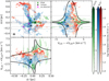 |
Fig. 16 Integrated intensity and PV diagrams of the blue (blue color bar) and red (red color bar) velocity components seen in N2H+ (1–0), and of the H2CO (2–1) emission (green color bar). Top left: spatial distribution of N2H+ and H2CO emission in G351.77. Markers and dashed gray lines are the same as in Fig. 11. The intersection of the dashed black lines represent the center of the rotating and infalling modeled sphere (see Appendix F). The ellipse in the bottom left represents the beam size of the N2H+ data. Top right and bottom left: PV diagrams along the two perpendicular directions. The black contours represent the shapes shown by the rotating and infalling modeled sphere in the PV diagram. |
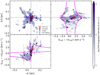 |
Fig. 17 Integrated intensity and PV diagrams of the DCN (3–2) emission. Top left: spatial distribution of DCN emission in G351.77. The green, black, and red × markers indicate the position of the dense cores (Louvet et al. 2024), where green and black represent the Cunningham et al. (2023) DCN spectral classification: single, and complex, respectively, and red indicates hot cores (also complex Bonfand et al. 2024). The blue stars indicate the position of the cataloged SiO outflows in G351.77, which are not associated with observed PV-features neither to range of velocities of DCN (Towner et al. 2024). The intersection of the dashed black curves represent the center of the rotating modeled sphere (see Appendix F). Top right and bottom left: PV diagrams along the two perpendicular directions. The magenta contours represent the PV features produced by a rotating modeled sphere in the PV diagram. |
7 Conclusions
We have conducted an analysis of the kinematics of the dense and cold gas within the massive G351.77 protocluster, traced by the spectral line N2H+ (1–0), utilizing the PV diagrams and characterization of physical processes involved in high-mass star formation. The spatial resolution of the N2H+ data cube is ~4 kau, making this the first study of its kind in G351.77.
Through spectral line fitting, we have obtained the main accessible physical parameters, such as excitation temperature, optical depth, centroid velocity, and line widths (see Sect. 3). We have implemented the spectral line fitting over the entire data cube, fitting one and two velocity components (see Sects. 3.1 and 3.2). We developed a method to identify and extract each spectra with one or two velocity components based on the line width and S/N of the modeled spectra (see Sect. 3.3). We finally obtained modeled data that possess spectra with one or two velocity components. Based on the centroid velocity distribution of each spectrum, we divided and isolated the data into two velocity components, which we named the blue velocity component and the red velocity component (see Sect. 3.4).
The excitation temperature, optical depth, and line widths enable the estimation of column density maps and masses of N2H+ (see Sect. 4). Additionally, we utilized the column density map of H2 provided by Dell’Ova et al. (2024) to estimate the relative abundance of N2H+, X(N2H+) ~ (1.66 ± 0.46) × 10−10, from which we derived an estimated total mass in the N2H+ emitting gas in the protocluster of ~1660 ± 326 M⊙.
The characterization of kinematic patterns, our main goal in this paper, revealed by the scrutiny of both the PV and PPV diagrams cubes, has allowed us to identify different small- and large-scale features (see Sect. 5). Our main results are:
The PV diagram on small scales reveals features such as V- and straight shapes associated in position and in velocity with the dense cores (Cunningham et al. 2023; Louvet et al. 2024). We suggest that the V-shapes describe inflowing gas in filamentary structures, where the dense cores are located near the vertex of the V-shapes. The straight shapes, on the other hand, describe inflowing filamentary structures going to denser N2H+ regions with dense cores following the stream produced by the gas (see Fig. 12);
We characterized these PV features by measuring the VGs, timescales, mass, and
![$\[\dot{\mathrm{M}}_{\text {tot,in}}\]$](/articles/aa/full_html/2025/04/aa52589-24/aa52589-24-eq20.png) . The most prominent V-shape reaches velocities of ~ −4.5 km s−1 relative to the VLSR, has an average
. The most prominent V-shape reaches velocities of ~ −4.5 km s−1 relative to the VLSR, has an average ![$\[\dot{\mathrm{M}}_{\text {tot,in}}\]$](/articles/aa/full_html/2025/04/aa52589-24/aa52589-24-eq21.png) of ~13.45 × 10⁻⁴ M⊙ yr−1, and a timescale of ~11.42 kyr (see Sect. 5.1);
of ~13.45 × 10⁻⁴ M⊙ yr−1, and a timescale of ~11.42 kyr (see Sect. 5.1);The above V-shapes have similar properties to the ones analyzed in Álvarez-Gutiérrez et al. (2024) in G353.41, indicating that they may be ubiquitous in this stage of protocluster evolution;
Similarly, we also find V- and straight shapes without associated dense cores; these have similar properties (timescales and
![$\[\dot{\mathrm{M}}_{\text {tot,in}}\]$](/articles/aa/full_html/2025/04/aa52589-24/aa52589-24-eq22.png) ) to the above sample. We suggest that these arise from possible cores or accretion centers that are under the detection limit of the 1.3 mm data (see Sect. 5.1 and Table E.1);
) to the above sample. We suggest that these arise from possible cores or accretion centers that are under the detection limit of the 1.3 mm data (see Sect. 5.1 and Table E.1);The averaged tf f of the dense cores is shorter than the timescales of the V-shapes. This suggests that the mass of the dense cores is increasing over their lifetimes, in turn modifying the tf f itself and likely driving faster dense core collapse;
The estimated timescales for the V-shapes are shorter than the timescale estimates for protostellar core envelope evolution (Valeille-Manet et al. 2025, and references therein). This suggests that the V-shapes are short-lived accretion signatures, which are more easily detectable in the most intense mass buildup phase of core formation. Hence, we can expect fewer V-shapes as star-forming regions evolve (see Sect. 5.1);
The total V-shape
![$\[\dot{\mathrm{M}}_{\text {tot,in}}\]$](/articles/aa/full_html/2025/04/aa52589-24/aa52589-24-eq23.png) (summed over the sample) enables us to estimate a depletion timescale of ~0.3 Myr in the protocluster. This implies a fast cluster formation timescale and/or a continuous mass feeding (see Sect. 5.1);
(summed over the sample) enables us to estimate a depletion timescale of ~0.3 Myr in the protocluster. This implies a fast cluster formation timescale and/or a continuous mass feeding (see Sect. 5.1);The PV diagram of N2H+ (on the largest scale we study of ~1.2 pc) reveals two main filamentary structures within the protocluster (F1 and F2 in Fig. 15). These filamentary structures are actively participating in the dense core and star formation, but at different levels, so we infer that they are at different evolutionary stages (see Sect. 5.2). This is consistent with previous findings of indications of different episodes of star formation in the ALMA-IMF protoclusters (Cunningham et al. 2023);
The analysis of large-scale VGs reveals that one of the two main filamentary structures (F1 in Fig. 15) may be inflowing toward a dense core position, where we observe the most prominent V-shape in the PV diagram at small scales (see above and Fig. 12). Within this filamentary structure, we find dense cores and PV features that are not associated with detected cores (see above). These seem to be inflowing along the filament (see Sect. 5.2);
The large-scale PV and PPV features seem to indicate that the protocluster is being fed by the Mother Filament (see Sect. 5.2), which the protocluster is forming out of.
The kinematic evidence observed in the dense gas, along with its characterization, suggests that G351.77 is actively and vigorously forming dense cores. However, based on the comparison with the G354.41 protocluster (Álvarez-Gutiérrez et al. 2024), the low SFR measured along the filament (Reyes-Reyes et al. 2024), and its consistency with the GHC scenario (Vázquez-Semadeni et al. 2019), we conclude that G351.77 protocluster is still in an early evolutionary stage. As the protocluster continues to be fed by the Mother Filament, we might expect to observe an increase in the number of cores, V-shaped features associated with them, and filamentary structures evolving into well-defined filaments, along with a rise in the SFR.
We have complemented the PV diagram analysis with the H2CO (2–1) and DCN (3–2) tracers, which cover areas without N2H+ (1–0) emission. This allows us to explore the relation between the large-scale kinematics described by N2H+ and the central region of the protocluster. In addition, we have implemented a rotating and infalling sphere model in order to characterize the PV features in the PV diagram produced by these kinematic processes, which is consistent with previous work (e.g., Tobin et al. 2012; Henshaw et al. 2014; Mori et al. 2024).
Here, in brief, we find that our simple toy model is consistent with larger-scale slow contraction and inner rotation, implying outside-in evolution as the initial angular momentum, possibly induced by Galactic shear (Braine et al. 2018, 2020), is dissipated (see also Álvarez-Gutiérrez et al. 2021). The PV features in the PV diagram produced by H2CO and DCN suggest that the central region of the protocluster may be experiencing simultaneous rotation and inflow, where the rotation appears to be the most dominant kinematic effect in the center (see Sect. 6.5). On the other hand, considering the velocity distribution and the position-position of the two large-scale velocity structures of N2H+ separated by ~2 km s−1 in the PV diagram, in addition to the possible rotation features described by H2CO and DCN, we suggest that these two large-scale velocity structures could be rotating relative to each other, with the rotating axis parallel to the direction of the Mother Filament. However, the most prominent kinematic process present at the N2H+ filamentary structures appears to be inflow, which seem to be inflowing not toward the center of the protocluster but rather inflowing onto themselves toward denser N2H+ regions (see Fig. 16).
Nevertheless, while the shapes and features presented in the model are consistent with the ones observed in the PV diagram by the tracers, the measured velocities exhibit an inconsistency with the velocities returned by the models by a factor of 3 (see Sect. 6.5). We attribute these differences to the simplicity of the toy model, which only considers two kinematic effects. At the same time, other works suggest the presence of rotation and infall at small scales, bipolar outflows produced by YSOs, gravitational instabilities along the filament, and magnetic fields in the protocluster, whose physical effect could be strongly affecting the behavior of the gas.
We have carried out a thorough analysis of the N2H+ line emission. One absolute imperative arising from this work is to ascertain the relationship of the protocluster to the Mother Filament (Reyes-Reyes et al. 2024) and the kinematic state of this filament as a whole. This work will be carried out in the near future.
Acknowledgements
We thank the referee for carefully comments, which helped improve this paper. This paper makes use of the following ALMA data: ADS/JAO.ALMA#2017.1.01355.L, #2013.1.01365.S, and #2015.1.01273.S. ALMA is a partnership of ESO (representing its member states), NSF (USA) and NINS (Japan), together with NRC (Canada), MOST and ASIAA (Taiwan), and KASI (Republic of Korea), in cooperation with the Republic of Chile. The Joint ALMA Observatory is operated by ESO, AUI/NRAO and NAOJ. The project leading to this publication has received support from ORP, which is funded by the European Union’s Horizon 2020 research and innovation program under grant agreement No. 101004719 [ORP]. This project has received funding from the European Research Council (ERC) via the ERC Synergy Grant ECOGAL (grant 855130) and from the French Agence Nationale de la Recherche (ANR) through the project COSMHIC (ANR-20-CE31-0009). A.S. gratefully acknowledges support by the Fondecyt Regular (project code 1220610), and ANID BASAL project FB210003. R.A. gratefully acknowledges support from ANID Beca Doctorado Nacional 21200897. R.G.M. acknowledges support from UNAM-PAPIIT project IN108822 and from CONAHCyT Ciencia de Frontera project ID 86372. Part of this work was performed at the high-performance computers at IRyAUNAM. T.Cs. and M.B. have received financial support from the French State in the framework of the IdEx Université de Bordeaux Investments for the future Program. A.G. acknowledges support from the NSF under grants AST 2008101 and CAREER 2142300. M.B. is a postdoctoral fellow in the University of Virginia’s VICO collaboration and is funded by grants from the NASA Astrophysics Theory Program (grant num- ber 80NSSC18K0558) and the NSF Astronomy & Astrophysics program (grant number 2206516). P.S. was partially supported by a Grant-in-Aid for Scientific Research (KAKENHI Number JP22H01271 and JP23H01221) of JSPS. R.A. gratefully acknowledges support from ANID Beca Doctorado Nacional 21200897. A.K. and L.B. gratefully acknowledges support from ANID BASAL project FB210003. S.R. acknowledges the funding and support of ANID-Subdirección de Capital Humano Magíster/Nacional/2021-22211000. G.B. acknowledge support from the PID2020-117710GB-I00 grant funded by MCIN/AEI(10.13039/501100011033 A.G. acknowledges the support of the Programme National ‘Physique et Chimie du Milieu Interstellaire’ (PCMI) of CNRS/INSU with INC/INP co-funded by CEA and CNES. H.-L. Liu is supported by Yunnan Fundamental Research Project (grant No. 202301AT070118, 202401AS070121). This work is supported by the China-Chile Joint Research Fund (CCJRF No. 2312). CCJRF is provided by Chinese Academy of Sciences South America Center for Astronomy (CASSACA) and established by National Astronomical Observatories, Chinese Academy of Sciences (NAOC) and Chilean Astronomy Society (SOCHIAS) to support China-Chile collaborations in astronomy. P. García is sponsored by the Chinese Academy of Sciences (CAS), through a grant to the CAS South America Center for Astronomy (CASSACA).
Appendix A N2H+ raw data
Figure A.1 displays different emission channels of the N2H+ (1–0) spectral line through the data cube observed with ALMA (see Sect. 2). Out of the 215 channels of the data cube, there are 110 that correspond to emission channels, which goes from -13.35 to 11.72 km s−1, with a spectral line resolution of 0.23 km s−1.
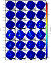 |
Fig. A.1 Channels map of data cube of the N2H+ (1–0) spectral line emission. There is a delta of velocity of 0.92 km s−1 between each channel. The velocities of each panel correspond to VLSR - <VLSR>. |
Appendix B PySpecKit experiment
To evaluate the performance of PySpecKit and determine the S/N threshold at which it provides reliable results, we conducted the following test: 1) We select a single spectrum from the data cube, from regions with S/N > 20, to fit it employing PySpecKit (with defined guesses and limits), obtaining a model and its respective parameters (input model). 2) We create a grid using this model, assigning a different S/N to each spectrum in the grid, artificially adding noise. 3) We fit the grid with PySpecKit (using the same guesses and limits as before), obtaining a new model for each spectrum (output models). By comparing parameters such as excitation temperature (Tex), optical depth (τ), centroid velocity (VLSR), and line width (σv) returned from the single spectrum (input model) versus the parameters returned from the grid (output model), we could assess the consistency of PySpecKit’s performance. This process was repeated for different spectra from the data cube, fitting one and two velocity components, conducting more than 200 different tests. The results of this experiment are consistent for both one- and two-velocity-components fits, showing that PySpecKit returns reliable values for S/N > 9. In contrast, for spectra with S/N < 9, the difference between the parameters from the input model and output models increases significantly, reaching values three or more times the standard deviation. Additionally, the uncertainties for each parameter rise to over the 30%, as expected. Figure B.1 shows the centroid velocity for the input and output models at different S/N levels, whose parameter exhibits the lowest uncertainties.
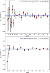 |
Fig. B.1 Example of the experiment fitting one velocity component (top) and two velocity components (bottom). The red points represent the centroid velocity value of the output models. The solid blue line shows the centroid velocity of the input model, while the dashed blue lines represent the range of the associated error. The error values increase as the S/N decreases. The discrepancy between the centroid velocity values of the output models and the input model increases as the S/N decreases, as we expected. |
Appendix C PySpecKit parameters
The models returned by PySpecKit produce parameter maps of the excitation temperature (Tex), optical depth (τ), centroid velocity (VLSR), and line width (σv) for each velocity component fit. Figures C.1 and C.2 show the Tex and τ maps for the blue and red velocity component defined in Sect. 3.4, while Figs. 6 and 7 display the centroid velocity and line width maps for both same velocity components (see Sect. 3.4), respectively.
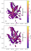 |
Fig. C.1 Top: Excitation temperature map of the blue velocity component. Bottom: Excitation temperature map of the red velocity component. The spectra inside the black contour are fit with two velocity components. The ellipse in the bottom left corner represents the beam size of the N2H+ data. |
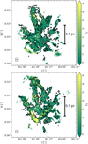 |
Fig. C.2 Top: Optical depth map of the blue velocity component. Bottom: Optical depth map of the red velocity component. The spectra inside the black contour are fit with two velocity components. The ellipse in the bottom left corner represents the beam size of the N2H+ data. |
Appendix D Good and bad fitting examples
The two-velocity-components fit of the N2H+ emission in G351.77 protocluster provides a more reliable fit for spectra that present multiple velocity components. However, this forces PySpecKit to fit “false velocity components” in spectra that reveal only one clear velocity component (see Fig. D.1 and Fig. D.2). The two methods applied over the model fit with one and two velocity components (see Sect. 3.3) enable us to define the best fit for each spectrum (see Fig. 4).
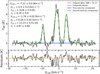 |
Fig. D.1 Example of two-velocity-components fits. The N2H+ data is represented by the histogram with their corresponding fits (colored curves), and the residuals are shown on the bottom panel. The orange line refers to the nil value. The modeled first velocity component has a σv,1 = 0 km s−1 and no uncertainties in its parameters, indicating that it is not possible to fit two velocity components in the spectrum. |
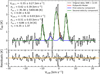 |
Fig. D.2 Example of two-velocity-components fits. The N2H+ data is represented by the histogram with their corresponding fits (colored curves), and the residuals are shown on the bottom panel. The orange line refers to the nil value. The intensity peak of the first velocity component is similar as what we measure for noise, indicating that it is not possible to fit two velocity components in the spectrum. |
Appendix E PV features at small scales
The characterization of the small-scale PV features observed in the PV diagram includes their position-position coordinates, shapes, velocity gradients, timescales, masses, and mass inflow rates.
Characterizations of the N2H+ PV features at small scale observed PV diagram.
Appendix F Infalling and rotating sphere model
Figure F.1 displays the modeled sphere under a Keplerian rotation (see Eq. 7) and its PV features produced in the PV diagrams. Figure F.2 represent the infalling modeled sphere (see Eq. 7) and its PV features produced in the PV diagrams. Figure F.3 represent the modeled sphere under both Keplerian rotation and infall at the same time and its PV features observed in the PV diagrams. The figures Fig. F.4, Fig. F.5, Fig. F.6, Fig. F.7, and Fig. F.8 display the H2CO and DCN spectral lines and its PV features observed in the PV diagrams, along with the PV features produced by the modeled sphere.
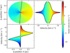 |
Fig. F.1 Top left: Position-position of a rotation-only sphere of 2700 M⊙. The solid black line represents the rotating axis whose inclination is of 85° respect to the x axis. Top right and bottom left: PV diagrams. The color bar represent the radial velocities derived from the Eq. 7, while the black contours show the PV features. |
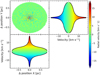 |
Fig. F.2 Top left: Position-position of an infalling-only sphere of 2700 M⊙. Top right and bottom left: PV diagrams. The color bar represent the radial velocities derived from the Eq. 7, while the black contours show the PV features. |
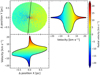 |
Fig. F.3 Top left: Position-position of a rotating and infalling sphere of 2700 M⊙. The solid black line represent the rotating axis whose inclination is of 85° respect to the x axis. Top right and bottom left: PV diagrams. The color bar represent the radial velocities derived from the Eq. 7, while the black contours show the PV features. |
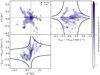 |
Fig. F.4 Same as Fig. 17 with the black contours represent the PV features produced by a rotating and infalling modeled sphere in the PV diagram. |
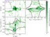 |
Fig. F.5 Integrated intensity and PV diagrams of the H2CO emission. Top left: Spatial distribution of H2CO emission in G351.77. The blue and magenta × markers indicate the position of the dense cores (Louvet et al. 2024), where each color represents the Cunningham et al. (2023) DCN spectral classification: single, and non-detected, respectively. Dashed gray curves indicate the positions of the dense cores that do not have identifiable velocities (non-detected). The intersection of the dashed black curves represent the center of the rotating and infalling modeled sphere (see Appendix F). Top right and bottom left: PV diagrams along the two perpendicular directions. The black contours represent the PV features produced by a rotating and infalling modeled sphere in the PV diagram. |
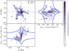 |
Fig. F.6 Same as Fig. 17 with the blue contours represent the PV features produced by a infalling modeled sphere in the PV diagram. |
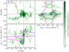 |
Fig. F.7 Same as Fig. F.5 with the magenta contours represent the PV features produced by a rotating modeled sphere in the PV diagram. |
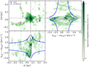 |
Fig. F.8 Same as Fig. F.5 with the blue contours represent the PV features produced by a infalling modeled sphere in the PV diagram. |
References
- Álvarez-Gutiérrez, R. H., Stutz, A. M., Law, C. Y., et al. 2021, ApJ, 908, 86 [CrossRef] [Google Scholar]
- Álvarez-Gutiérrez, R. H., Stutz, A. M., Sandoval-Garrido, N., et al. 2024, A&A, 689, A74 [NASA ADS] [CrossRef] [EDP Sciences] [Google Scholar]
- André, P., Arzoumanian, D., Könyves, V., Shimajiri, Y., & Palmeirim, P. 2019, A&A, 629, L4 [Google Scholar]
- Antyufeyev, O. V., Shulga, V. M., & Zinchenko, I. I. 2016, Kinematics Phys. Celest. Bodies, 32, 276 [Google Scholar]
- Anirudh, R., Eswaraiah, C., Jiao, S., & Jose, J. 2023, J. Astrophys. Astron., 44, 59 [Google Scholar]
- Armante, M., Gusdorf, A., Louvet, F., et al. 2024, A&A, 686, A122 [NASA ADS] [CrossRef] [EDP Sciences] [Google Scholar]
- Arzoumanian, D., Arakawa, S., Kobayashi, M. I. N., et al. 2023, ApJ, 947, L29 [Google Scholar]
- Bally, J., Langer, W. D., Stark, A. A., & Wilson, R. W. 1987, ApJ, 312, L45 [NASA ADS] [CrossRef] [Google Scholar]
- Bergin, E. A., & Tafalla, M. 2007, ARA&A, 45, 339 [Google Scholar]
- Bergin, E. A., Ciardi, D. R., Lada, C. J., Alves, J., & Lada, E. A. 2001, ApJ, 557, 209 [NASA ADS] [CrossRef] [Google Scholar]
- Beuther, H., Walsh, A. J., Johnston, K. G., et al. 2017, A&A, 603, A10 [NASA ADS] [CrossRef] [EDP Sciences] [Google Scholar]
- Bonfand, M., Csengeri, T., Bontemps, S., et al. 2024, A&A, 687, A163 [NASA ADS] [CrossRef] [EDP Sciences] [Google Scholar]
- Bonne, L., Bontemps, S., Schneider, N., et al. 2020, A&A, 644, A27 [EDP Sciences] [Google Scholar]
- Braine, J., Rosolowsky, E., Gratier, P., Corbelli, E., & Schuster, K. F. 2018, A&A, 612, A51 [NASA ADS] [CrossRef] [EDP Sciences] [Google Scholar]
- Braine, J., Hughes, A., Rosolowsky, E., et al. 2020, A&A, 633, A17 [NASA ADS] [CrossRef] [EDP Sciences] [Google Scholar]
- Brouillet, N., Despois, D., Molet, J., et al. 2022, A&A, 665, A140 [NASA ADS] [CrossRef] [EDP Sciences] [Google Scholar]
- Busquet, G., Estalella, R., Zhang, Q., et al. 2011, A&A, 525, A141 [NASA ADS] [CrossRef] [EDP Sciences] [Google Scholar]
- CASA Team (Bean, B., et al.) 2022, PASP, 134, 114501 [NASA ADS] [CrossRef] [Google Scholar]
- Caselli, P., Myers, P. C., & Thaddeus, P. 1995, ApJ, 455, L77 [Google Scholar]
- Caselli, P., Benson, P. J., Myers, P. C., & Tafalla, M. 2002a, ApJ, 572, 238 [Google Scholar]
- Caselli, P., Walmsley, C. M., Zucconi, A., et al. 2002b, ApJ, 565, 331 [NASA ADS] [CrossRef] [Google Scholar]
- Caselli, P., Walmsley, C. M., Zucconi, A., et al. 2002c, ApJ, 565, 344 [Google Scholar]
- Chen, H.-R. V., Zhang, Q., Wright, M. C. H., et al. 2019, ApJ, 875, 24 [Google Scholar]
- Cunningham, N., Ginsburg, A., Galván-Madrid, R., et al. 2023, A&A, 678, A194 [NASA ADS] [CrossRef] [EDP Sciences] [Google Scholar]
- Dale, J. E., Ngoumou, J., Ercolano, B., & Bonnell, I. A. 2014, MNRAS, 442, 694 [Google Scholar]
- Daniel, F., Dubernet, M. L., Meuwly, M., Cernicharo, J., & Pagani, L. 2005, MNRAS, 363, 1083 [NASA ADS] [CrossRef] [Google Scholar]
- Dell’Ova, P., Motte, F., Gusdorf, A., et al. 2024, A&A, 687, A217 [NASA ADS] [CrossRef] [EDP Sciences] [Google Scholar]
- Díaz-González, D. J., Galván-Madrid, R., Ginsburg, A., et al. 2023, ApJS, 269, 55 [CrossRef] [Google Scholar]
- Dib, S., Zhou, J.-W., Comerón, S., et al. 2025, A&A, 693, A51 [NASA ADS] [CrossRef] [EDP Sciences] [Google Scholar]
- Fernández-López, M., Arce, H. G., Looney, L., et al. 2014, ApJ, 790, L19 [Google Scholar]
- Fontani, F., Caselli, P., Crapsi, A., et al. 2006, A&A, 460, 709 [NASA ADS] [CrossRef] [EDP Sciences] [Google Scholar]
- Galván-Madrid, R., Keto, E., Zhang, Q., et al. 2009, ApJ, 706, 1036 [CrossRef] [Google Scholar]
- Galván-Madrid, R., Zhang, Q., Keto, E., et al. 2010, ApJ, 725, 17 [Google Scholar]
- Galván-Madrid, R., Díaz-González, D. J., Motte, F., et al. 2024, ApJS, 274, 15 [CrossRef] [Google Scholar]
- Ginsburg, A., & Mirocha, J. 2011, PySpecKit: Python Spectroscopic Toolkit, Astrophysics Source Code Library [record ascl:1109.001] [Google Scholar]
- Ginsburg, A., Csengeri, T., Galván-Madrid, R., et al. 2022a, A&A, 662, A9 [NASA ADS] [CrossRef] [EDP Sciences] [Google Scholar]
- Ginsburg, A., Sokolov, V., de Val-Borro, M., et al. 2022b, AJ, 163, 291 [NASA ADS] [CrossRef] [Google Scholar]
- González Lobos, V., & Stutz, A. M. 2019, MNRAS, 489, 4771 [CrossRef] [Google Scholar]
- Green, S., Montgomery, J. A., J., & Thaddeus, P. 1974, ApJ, 193, L89 [Google Scholar]
- Guerrero-Gamboa, R., & Vázquez-Semadeni, E. 2020, ApJ, 903, 136 [NASA ADS] [CrossRef] [Google Scholar]
- Hacar, A., & Tafalla, M. 2011, A&A, 533, A34 [NASA ADS] [CrossRef] [EDP Sciences] [Google Scholar]
- Hacar, A., Alves, J., Tafalla, M., & Goicoechea, J. R. 2017, A&A, 602, L2 [NASA ADS] [CrossRef] [EDP Sciences] [Google Scholar]
- Hacar, A., Clark, S. E., Heitsch, F., et al. 2023, in Astronomical Society of the Pacific Conference Series, 534, Protostars and Planets VII, eds. S. Inutsuka, Y. Aikawa, T. Muto, K. Tomida, & M. Tamura, 153 [Google Scholar]
- Hacar, A., Socci, A., Bonanomi, F., et al. 2024, A&A, 687, A140 [NASA ADS] [CrossRef] [EDP Sciences] [Google Scholar]
- Haworth, T. J., Shima, K., Tasker, E. J., et al. 2015, MNRAS, 454, 1634 [NASA ADS] [CrossRef] [Google Scholar]
- Henshaw, J. D., Caselli, P., Fontani, F., Jiménez-Serra, I., & Tan, J. C. 2014, MNRAS, 440, 2860 [Google Scholar]
- Issac, N., Tej, A., Liu, T., & Wu, Y. 2020, MNRAS, 499, 3620 [NASA ADS] [CrossRef] [Google Scholar]
- Ivanov, D., Bu, C., Hillenbrand, P.-M., et al. 2024, in American Astronomical Society Meeting Abstracts, 244, 222.04 [Google Scholar]
- Izquierdo, A. F., Galván-Madrid, R., Maud, L. T., et al. 2018, MNRAS, 478, 2505 [NASA ADS] [CrossRef] [Google Scholar]
- Jørgensen, J. K., Schöier, F. L., & van Dishoeck, E. F. 2004, A&A, 416, 603 [Google Scholar]
- Kim, S., Lee, C. W., Tafalla, M., et al. 2022, ApJ, 940, 112 [NASA ADS] [CrossRef] [Google Scholar]
- Kirk, J. M., Ward-Thompson, D., Di Francesco, J., et al. 2024, MNRAS, 532, 4661 [NASA ADS] [CrossRef] [Google Scholar]
- Klaassen, P. D., Johnston, K. G., Leurini, S., & Zapata, L. A. 2015, A&A, 575, A54 [NASA ADS] [CrossRef] [EDP Sciences] [Google Scholar]
- Kong, S., Whitworth, D. J., Smith, R. J., & Hamden, E. T. 2022, MNRAS, 517, 4679 [Google Scholar]
- Lada, C. J., & Lada, E. A. 2003, ARA&A, 41, 57 [Google Scholar]
- Lee, Y.-N., & Hennebelle, P. 2016, A&A, 591, A30 [NASA ADS] [CrossRef] [EDP Sciences] [Google Scholar]
- Lee, K. I., Fernández-López, M., Storm, S., et al. 2014, ApJ, 797, 76 [Google Scholar]
- Leurini, S., Hieret, C., Thorwirth, S., et al. 2008, A&A, 485, 167 [NASA ADS] [CrossRef] [EDP Sciences] [Google Scholar]
- Leurini, S., Codella, C., Zapata, L., et al. 2011a, A&A, 530, A12 [NASA ADS] [CrossRef] [EDP Sciences] [Google Scholar]
- Leurini, S., Pillai, T., Stanke, T., et al. 2011b, A&A, 533, A85 [NASA ADS] [CrossRef] [EDP Sciences] [Google Scholar]
- Leurini, S., Codella, C., Gusdorf, A., et al. 2013, A&A, 554, A35 [NASA ADS] [CrossRef] [EDP Sciences] [Google Scholar]
- Leurini, S., Gusdorf, A., Wyrowski, F., et al. 2014, A&A, 564, L11 [NASA ADS] [CrossRef] [EDP Sciences] [Google Scholar]
- Leurini, S., Schisano, E., Pillai, T., et al. 2019, A&A, 621, A130 [NASA ADS] [CrossRef] [EDP Sciences] [Google Scholar]
- Li, X.-M., Zhang, G.-Y., Men’shchikov, A., et al. 2023, A&A, 674, A225 [NASA ADS] [CrossRef] [EDP Sciences] [Google Scholar]
- Lippok, N., Launhardt, R., Semenov, D., et al. 2013, A&A, 560, A41 [NASA ADS] [CrossRef] [EDP Sciences] [Google Scholar]
- Liu, H. B., Galván-Madrid, R., Jiménez-Serra, I., et al. 2015, ApJ, 804, 37 [Google Scholar]
- Liu, H.-L., Stutz, A., & Yuan, J.-H. 2019, MNRAS, 487, 1259 [Google Scholar]
- Liu, H.-L., Sanhueza, P., Liu, T., et al. 2020, ApJ, 901, 31 [NASA ADS] [CrossRef] [Google Scholar]
- Liu, H.-L., Tej, A., Liu, T., et al. 2023, MNRAS, 522, 3719 [NASA ADS] [CrossRef] [Google Scholar]
- Louvet, F., Motte, F., Gusdorf, A., et al. 2016, A&A, 595, A122 [NASA ADS] [CrossRef] [EDP Sciences] [Google Scholar]
- Louvet, F., Sanhueza, P., Stutz, A., et al. 2024, A&A, 690, A33 [NASA ADS] [CrossRef] [EDP Sciences] [Google Scholar]
- Lu, X., Zhang, Q., Liu, H. B., et al. 2018, ApJ, 855, 9 [Google Scholar]
- Mangum, J. G., & Shirley, Y. L. 2017, PASP, 129, 069201 [NASA ADS] [CrossRef] [Google Scholar]
- Maret, S., Ceccarelli, C., Caux, E., et al. 2004, A&A, 416, 577 [NASA ADS] [CrossRef] [EDP Sciences] [Google Scholar]
- Men’shchikov, A. 2021, A&A, 649, A89 [EDP Sciences] [Google Scholar]
- Minh, Y. C., Liu, H. B., Galvań-Madrid, R., et al. 2018, ApJ, 864, 102 [NASA ADS] [CrossRef] [Google Scholar]
- Montillaud, J., Juvela, M., Vastel, C., et al. 2019, A&A, 631, A3 [NASA ADS] [CrossRef] [EDP Sciences] [Google Scholar]
- Mori, S., Aikawa, Y., Oya, Y., Yamamoto, S., & Sakai, N. 2024, ApJ, 961, 31 [Google Scholar]
- Motte, F., Bontemps, S., & Louvet, F. 2018, ARA&A, 56, 41 [NASA ADS] [CrossRef] [Google Scholar]
- Motte, F., Bontemps, S., Csengeri, T., et al. 2022, A&A, 662, A8 [NASA ADS] [CrossRef] [EDP Sciences] [Google Scholar]
- Motte, F., Pouteau, Y., Nony, T., et al. 2025, A&A, 694, A24 [NASA ADS] [CrossRef] [EDP Sciences] [Google Scholar]
- Nony, T., Galván-Madrid, R., Motte, F., et al. 2023, A&A, 674, A75 [NASA ADS] [CrossRef] [EDP Sciences] [Google Scholar]
- Pagani, L., Daniel, F., & Dubernet, M.-L. 2008, On the frequency of N2H+ and N2D+, https://hal.science/hal-00340115v1 [Google Scholar]
- Pan, S., Liu, H.-L., & Qin, S.-L. 2024, ApJ, 960, 76 [NASA ADS] [CrossRef] [Google Scholar]
- Peretto, N., & Fuller, G. A. 2009, A&A, 505, 405 [NASA ADS] [CrossRef] [EDP Sciences] [Google Scholar]
- Pety, J., Guzmán, V. V., Orkisz, J. H., et al. 2017, A&A, 599, A98 [NASA ADS] [CrossRef] [EDP Sciences] [Google Scholar]
- Pirogov, L. E., Zemlyanukha, P. M., Dombek, E. M., & Voronkov, M. A. 2023, Astron. Rep., 67, 1355 [Google Scholar]
- Plunkett, A. L., Fernández-López, M., Arce, H. G., et al. 2018, A&A, 615, A9 [NASA ADS] [CrossRef] [EDP Sciences] [Google Scholar]
- Pouteau, Y., Motte, F., Nony, T., et al. 2022, A&A, 664, A26 [NASA ADS] [CrossRef] [EDP Sciences] [Google Scholar]
- Pouteau, Y., Motte, F., Nony, T., et al. 2023, A&A, 674, A76 [NASA ADS] [CrossRef] [EDP Sciences] [Google Scholar]
- Priestley, F. D., Clark, P. C., Glover, S. C. O., et al. 2023, MNRAS, 526, 4952 [NASA ADS] [CrossRef] [Google Scholar]
- Redaelli, E., Bizzocchi, L., Caselli, P., et al. 2019, A&A, 629, A15 [NASA ADS] [CrossRef] [EDP Sciences] [Google Scholar]
- Redaelli, E., Bovino, S., Sanhueza, P., et al. 2022, ApJ, 936, 169 [NASA ADS] [CrossRef] [Google Scholar]
- Reyes-Reyes, S. D., Stutz, A. M., Megeath, S. T., et al. 2024, MNRAS, 529, 2220 [NASA ADS] [CrossRef] [Google Scholar]
- Sabatini, G., Giannetti, A., Bovino, S., et al. 2019, MNRAS, 490, 4489 [Google Scholar]
- Sanhueza, P., Jackson, J. M., Foster, J. B., et al. 2012, ApJ, 756, 60 [Google Scholar]
- Sanhueza, P., Girart, J. M., Padovani, M., et al. 2021, ApJ, 915, L10 [NASA ADS] [CrossRef] [Google Scholar]
- Schneider, N., Csengeri, T., Bontemps, S., et al. 2010, A&A, 520, A49 [CrossRef] [EDP Sciences] [Google Scholar]
- Schwarz, K. R., Teague, R., & Bergin, E. A. 2019, ApJ, 876, L13 [Google Scholar]
- Shirley, Y. L. 2015, PASP, 127, 299 [Google Scholar]
- Storm, S., Mundy, L. G., Fernández-López, M., et al. 2014, ApJ, 794, 165 [NASA ADS] [CrossRef] [Google Scholar]
- Stutz, A. M. 2018, MNRAS, 473, 4890 [NASA ADS] [CrossRef] [Google Scholar]
- Stutz, A. M., & Gould, A. 2016, A&A, 590, A2 [NASA ADS] [CrossRef] [EDP Sciences] [Google Scholar]
- Stutz, A. M., & Kainulainen, J. 2015, A&A, 577, L6 [NASA ADS] [CrossRef] [EDP Sciences] [Google Scholar]
- Stutz, A. M., Gonzalez-Lobos, V., & Gould, A. 2018, MNRAS, submitted, [arXiv:1807.11496] [Google Scholar]
- Tafalla, M., & Hacar, A. 2014, in Dense Cores: Origin, Evolution, and Collapse, 4, 103.01 [Google Scholar]
- Tatematsu, K., Kandori, R., Umemoto, T., & Sekimoto, Y. 2008, PASJ, 60, 407 [NASA ADS] [Google Scholar]
- Thaddeus, P., & Turner, B. E. 1975, ApJ, 201, L25 [Google Scholar]
- Tobin, J. J., Hartmann, L., Bergin, E., et al. 2012, ApJ, 748, 16 [Google Scholar]
- Tobin, J. J., Bergin, E. A., Hartmann, L., et al. 2013, ApJ, 765, 18 [NASA ADS] [CrossRef] [Google Scholar]
- Towner, A. P. M., Ginsburg, A., Dell’Ova, P., et al. 2024, ApJ, 960, 48 [NASA ADS] [CrossRef] [Google Scholar]
- Turner, B. E. 1974, ApJ, 193, L83 [Google Scholar]
- Valeille-Manet, M., Bontemps, S., Csengeri, T., et al. 2025, A&A, 696, A11 [NASA ADS] [CrossRef] [EDP Sciences] [Google Scholar]
- van’t Hoff, M. L. R., Walsh, C., Kama, M., Facchini, S., & van Dishoeck, E. F. 2017, A&A, 599, A101 [Google Scholar]
- Vázquez-Semadeni, E., Palau, A., Ballesteros-Paredes, J., Gómez, G. C., & Zamora-Avilés, M. 2019, MNRAS, 490, 3061 [Google Scholar]
- Vázquez-Semadeni, E., Hu, Y., Xu, S., Guerrero-Gamboa, R., & Lazarian, A. 2024, MNRAS, 530, 3431 [Google Scholar]
- Yang, D., Liu, H.-L., Tej, A., et al. 2023, ApJ, 953, 40 [NASA ADS] [CrossRef] [Google Scholar]
- Yu, N.-P., Xu, J.-L., Wang, J.-J., & Liu, X.-L. 2018, ApJ, 865, 135 [NASA ADS] [CrossRef] [Google Scholar]
- Zapata, L. A., Leurini, S., Menten, K. M., et al. 2008, AJ, 136, 1455 [Google Scholar]
- Zhou, J.-W., Liu, T., Evans, N. J., et al. 2022, MNRAS, 514, 6038 [NASA ADS] [CrossRef] [Google Scholar]
All Tables
All Figures
|
Fig. 1 The IRAC color composite image of the G351.77-0.53 filamentary region, where the 8.0 μm, 5.6 μm, and 3.6 μm are shown in red, green, and blue, respectively. The orange contour shows the coverage of the 3 mm data ALMA-IMF Large Program observations. The white contour represents the ATLASGAL emission (850 μm) at 0.62 Jy beam−1. The dominant central closed contour indicates the Mother Filament discussed below (also referred to as the “G351 filament” in Reyes-Reyes et al. 2024). This filament is also observed in NIR extinction and submillimeter emission. In its densest part, the star formation activity is revealed by strong NIR emission. |
| In the text | |
|
Fig. 2 Top: noise map of the fully combined N2H+ image (see text) in the G351.77 protocluster. The spectra with the highest noise values are located near the edges, as was expected. The mean rms value across the entire map is ~0.66 K, whereas the mean value in regions with S/N > 9 is ~0.40 K. Bottom: signal-to-noise ratio (S/N) map. Spectra with high S/N are distributed following filamentary structures. The contours show the areas where spectra with S/N ≥ 9 are found (see Appendix B). The ellipse in the bottom left corner represents the final beam size of the N2H+ data of 2.3″ × 2.1″, or 4.6 kau × 4.2 kau. |
| In the text | |
|
Fig. 3 Centroid velocity distributions of the one- and two-velocity-components fits. The black histogram represents the centroid velocity distribution of the spectra fit by the one-velocity-component model. The blue and red histograms show the centroid velocity distributions of the spectra fit with the two-velocity-components model, where blue corresponds to the first velocity component and red to the second velocity component. The solid black line represents the middle point X located at 0.025 km s−1, measured via Eq. (1) (see text). This divides the black histogram into two velocities, as explained in Sect. 3.4. |
| In the text | |
|
Fig. 4 Example of one-velocity (top) and two-velocity (bottom) component fits to two different spectra; the former (later) corresponds to a spectrum extracted from the blue (orange) areas in Fig. 5. In both panels: the data are represented on the top (solid black histograms) with their corresponding fits (colored curves), and the residuals are shown on the bottom, here the orange line refers to the nil value. The S/N of each spectrum, as well as the best-fit parameter values, are listed in each panel. In the bottom panel, the red curve represents the sum over the two velocity components. |
| In the text | |
|
Fig. 5 Map of the number of velocity components in the N2H+ (1–0) spectral fits in the G351.77 protocluster. The blue (orange) pixels represent 59% (41%) of the spectra where we adopt a one-velocity-component fit (two-velocity-components fit), see Sect. 3.3. Most of the orange pixels are located in central regions, where we observe the highest S/N and integrated intensity values, similar to the results for G353.41 (Álvarez-Gutiérrez et al. 2024). The blue areas are located preferentially near the edges. The ellipse in the bottom left corner represents the beam size of the N2H+ data. |
| In the text | |
|
Fig. 6 Top: integrated intensity map from the final spectral model composed of both the one and two velocity components. Middle: line width map of the blue velocity component. Bottom: line width map of the red velocity component. The spectra inside the black contour are fit with two velocity components. The ellipse in the bottom left corner represents the beam size of the N2H+ data. |
| In the text | |
|
Fig. 7 Top: mean velocity map from the final spectral model composed of both the one and two velocity components. The red arrow display the direction of the Mother Filament. The blue arrow indicates the direction of the large-scale velocity gradient measured from the centroid velocities. Middle: centroid velocity map of the blue velocity component. Bottom: centroid velocity map of the red velocity component. The spectra inside the black contour are fit with two velocity components. The ellipse in the bottom left corner represents the beam size of the N2H+ data. |
| In the text | |
|
Fig. 8 N2H+ total column density map derived from Eq. (2). The ellipse in the bottom left corner represents the beam size of the N2H+ data. |
| In the text | |
|
Fig. 9 H2 column density map from Dell’Ova et al. (2024) of the G351.77 protocluster. The black contour represents the spectra with NT(N2H+) > 1 × 1013 cm−2. The circle on the bottom left represents the beam size of 6″ × 6″. |
| In the text | |
|
Fig. 10 Relative abundance X(N2H+) distribution in the G351.77 protocluster zone. The dashed red line represents the mean of the distribution. The dashed black line represents the mean inside the most prominent bin of the distribution. The shaded region represents the estimated error around the mode. |
| In the text | |
|
Fig. 11 Integrated intensity and PV diagrams of the blue (blue color bar) and red (red color bar) velocity components seen in N2H+ (1–0). Top left: spatial distribution of N2H+ (1–0) emission in G351.77. The green, black, and magenta × markers indicate the positions of the 9 out of the 18 (see Sect. 5.1) dense cores (Louvet et al. 2024), where each color represents the DCN spectral classification: single, complex, and non-detected, respectively (Cunningham et al. 2023). The + markers indicate the position of the 16 core candidates, proposed on the basis on the N2H+ PV features observed at scales of ~0.1 pc (see Sect. 5.1 and Table E.1). Dashed lines indicate the positions of the four dense cores that do not have measurable velocities. The red arrow indicates the direction of the Mother Filament. The ellipse in the bottom left represents the beam size of the N2H+ data. Top right and bottom left: PV diagrams along the two perpendicular directions. Top right: the colored arrows indicate the position of the dense cores and their ID in Table 3. We observe multiple structures, such as V-shapes and Straight structures (see text) along the filaments, some associated with dense cores in both position and velocity. The orange arrows represent a velocity gradient of 10 km s−1 pc−1 ≈ 0.1 Myr. |
| In the text | |
|
Fig. 12 Top: PV diagram of the most prominent V-shape (L19 in Fig. 11). The black outlined points show the points used in order to generate the linear fits of the velocity gradients. The red and blue lines represent the upper and lower VG, respectively, which converge at ~ 0.015 pc below the central position of the dense core. The magenta error bar represents the projected size of the dense core (Louvet et al. 2024), while the horizontal dashed line represents the position of the dense core. The color bar shows the integrated intensity of N2H+ (1–0) levels. The gray error bar represents the beam size of the N2H+ data. The green arrow represents a velocity gradient of 25 km s−1 pc−1, which corresponds to a timescale of ~0.4 Myr. Middle: Position-position diagram of the most prominent V-shape. The squares represent the points used for the linear fit (top figure). The size of the squares correspond to the integrated intensity of each spectrum, while the ellipse indicates the position and size of the dense core (L19 in Fig. 11). Bottom right: Proposed model for the observed PV features as V-shapes (see also Fig. 12 in Henshaw et al. 2014 and Álvarez-Gutiérrez et al. 2024). Bottom left: inflowing filamentary structure. The light blue and blue arrows represent the velocity magnitude of the gas and the radial component of the gas velocity, respectively. Right: PV diagram of the model. |
| In the text | |
|
Fig. 13 PV diagram of a single core (L18 in Table E.1) from the catalog of Louvet et al. (2024). The PV feature outlines what we define as a straight shape. The black outlined points show the points used to generate the linear fit of the velocity gradient. The red line represents the linear fit of the velocity gradient. The green × marker indicates the position (Louvet et al. 2024) and velocity of the dense core measured in DCN (see Table F.9 in Cunningham et al. 2023), while the green bar indicates the projected dense core size. The gray error bar represents the beam size of the N2H+ data. The green arrow represents a velocity gradient of 25 km s−1 pc−1, which correspond to a timescale of ~0.4 Myr. |
| In the text | |
|
Fig. 14 PV diagram of the blue (blue color bar) and red (red color bar) velocity components seen in N2H+ (1–0). The dark points highlight the PV features observed. The blue arrows represent the location of the 16 PV features of candidates cores under the 1.3 mm band detection limit (see Table E.1). The red arrows indicate the location in the PV diagram of PV features associated with the dense cores (Louvet et al. 2024, see Table E.1). The markers and dashed lines are the same as in Fig. 11. The green arrow represents a velocity gradient of 10 km s−1 pc−1, which correspond to a timescale of 0.1 Myr. |
| In the text | |
|
Fig. 15 Integrated intensity and PV diagram of the F1 (blue color bar), F2 (red color bar), F3 (green color bar), and F4 (purple color bar) largescale structures of N2H+ (1–0) into which the protocluster has been divided. Left: Spatial distribution of N2H+ (1–0) emission. Markers and dashed lines are the same as in Fig. 11. The ellipse in the bottom left represents the beam size of the N2H+ data. Right: PV diagram. We observe multiple large-scale V-shapes and straight shapes along the different filamentary structures, with some of them associated with dense cores in position and in velocity. The green arrows represent a velocity gradient of 10 km s−1 pc−1, which correspond to a timescale of ~0.1 Myr. |
| In the text | |
|
Fig. 16 Integrated intensity and PV diagrams of the blue (blue color bar) and red (red color bar) velocity components seen in N2H+ (1–0), and of the H2CO (2–1) emission (green color bar). Top left: spatial distribution of N2H+ and H2CO emission in G351.77. Markers and dashed gray lines are the same as in Fig. 11. The intersection of the dashed black lines represent the center of the rotating and infalling modeled sphere (see Appendix F). The ellipse in the bottom left represents the beam size of the N2H+ data. Top right and bottom left: PV diagrams along the two perpendicular directions. The black contours represent the shapes shown by the rotating and infalling modeled sphere in the PV diagram. |
| In the text | |
|
Fig. 17 Integrated intensity and PV diagrams of the DCN (3–2) emission. Top left: spatial distribution of DCN emission in G351.77. The green, black, and red × markers indicate the position of the dense cores (Louvet et al. 2024), where green and black represent the Cunningham et al. (2023) DCN spectral classification: single, and complex, respectively, and red indicates hot cores (also complex Bonfand et al. 2024). The blue stars indicate the position of the cataloged SiO outflows in G351.77, which are not associated with observed PV-features neither to range of velocities of DCN (Towner et al. 2024). The intersection of the dashed black curves represent the center of the rotating modeled sphere (see Appendix F). Top right and bottom left: PV diagrams along the two perpendicular directions. The magenta contours represent the PV features produced by a rotating modeled sphere in the PV diagram. |
| In the text | |
|
Fig. A.1 Channels map of data cube of the N2H+ (1–0) spectral line emission. There is a delta of velocity of 0.92 km s−1 between each channel. The velocities of each panel correspond to VLSR - <VLSR>. |
| In the text | |
|
Fig. B.1 Example of the experiment fitting one velocity component (top) and two velocity components (bottom). The red points represent the centroid velocity value of the output models. The solid blue line shows the centroid velocity of the input model, while the dashed blue lines represent the range of the associated error. The error values increase as the S/N decreases. The discrepancy between the centroid velocity values of the output models and the input model increases as the S/N decreases, as we expected. |
| In the text | |
|
Fig. C.1 Top: Excitation temperature map of the blue velocity component. Bottom: Excitation temperature map of the red velocity component. The spectra inside the black contour are fit with two velocity components. The ellipse in the bottom left corner represents the beam size of the N2H+ data. |
| In the text | |
|
Fig. C.2 Top: Optical depth map of the blue velocity component. Bottom: Optical depth map of the red velocity component. The spectra inside the black contour are fit with two velocity components. The ellipse in the bottom left corner represents the beam size of the N2H+ data. |
| In the text | |
|
Fig. D.1 Example of two-velocity-components fits. The N2H+ data is represented by the histogram with their corresponding fits (colored curves), and the residuals are shown on the bottom panel. The orange line refers to the nil value. The modeled first velocity component has a σv,1 = 0 km s−1 and no uncertainties in its parameters, indicating that it is not possible to fit two velocity components in the spectrum. |
| In the text | |
|
Fig. D.2 Example of two-velocity-components fits. The N2H+ data is represented by the histogram with their corresponding fits (colored curves), and the residuals are shown on the bottom panel. The orange line refers to the nil value. The intensity peak of the first velocity component is similar as what we measure for noise, indicating that it is not possible to fit two velocity components in the spectrum. |
| In the text | |
|
Fig. F.1 Top left: Position-position of a rotation-only sphere of 2700 M⊙. The solid black line represents the rotating axis whose inclination is of 85° respect to the x axis. Top right and bottom left: PV diagrams. The color bar represent the radial velocities derived from the Eq. 7, while the black contours show the PV features. |
| In the text | |
|
Fig. F.2 Top left: Position-position of an infalling-only sphere of 2700 M⊙. Top right and bottom left: PV diagrams. The color bar represent the radial velocities derived from the Eq. 7, while the black contours show the PV features. |
| In the text | |
|
Fig. F.3 Top left: Position-position of a rotating and infalling sphere of 2700 M⊙. The solid black line represent the rotating axis whose inclination is of 85° respect to the x axis. Top right and bottom left: PV diagrams. The color bar represent the radial velocities derived from the Eq. 7, while the black contours show the PV features. |
| In the text | |
|
Fig. F.4 Same as Fig. 17 with the black contours represent the PV features produced by a rotating and infalling modeled sphere in the PV diagram. |
| In the text | |
|
Fig. F.5 Integrated intensity and PV diagrams of the H2CO emission. Top left: Spatial distribution of H2CO emission in G351.77. The blue and magenta × markers indicate the position of the dense cores (Louvet et al. 2024), where each color represents the Cunningham et al. (2023) DCN spectral classification: single, and non-detected, respectively. Dashed gray curves indicate the positions of the dense cores that do not have identifiable velocities (non-detected). The intersection of the dashed black curves represent the center of the rotating and infalling modeled sphere (see Appendix F). Top right and bottom left: PV diagrams along the two perpendicular directions. The black contours represent the PV features produced by a rotating and infalling modeled sphere in the PV diagram. |
| In the text | |
|
Fig. F.6 Same as Fig. 17 with the blue contours represent the PV features produced by a infalling modeled sphere in the PV diagram. |
| In the text | |
|
Fig. F.7 Same as Fig. F.5 with the magenta contours represent the PV features produced by a rotating modeled sphere in the PV diagram. |
| In the text | |
|
Fig. F.8 Same as Fig. F.5 with the blue contours represent the PV features produced by a infalling modeled sphere in the PV diagram. |
| In the text | |
Current usage metrics show cumulative count of Article Views (full-text article views including HTML views, PDF and ePub downloads, according to the available data) and Abstracts Views on Vision4Press platform.
Data correspond to usage on the plateform after 2015. The current usage metrics is available 48-96 hours after online publication and is updated daily on week days.
Initial download of the metrics may take a while.