| Issue |
A&A
Volume 689, September 2024
|
|
|---|---|---|
| Article Number | A74 | |
| Number of page(s) | 23 | |
| Section | Interstellar and circumstellar matter | |
| DOI | https://doi.org/10.1051/0004-6361/202450321 | |
| Published online | 04 September 2024 | |
ALMA-IMF
XIII. N2H+ kinematic analysis of the intermediate protocluster G353.41
1
Departamento de Astronomía, Universidad de Concepción,
Casilla 160-C,
Concepción,
Chile
e-mail: This email address is being protected from spambots. You need JavaScript enabled to view it.
2
Univ. Grenoble Alpes, CNRS, IPAG,
38000
Grenoble,
France
3
Instituto de Radioastronomía y Astrofísica, Universidad Nacional Autónoma de México,
Morelia,
Michoacán
58089,
Mexico
4
SKA Observatory, Jodrell Bank,
Lower Withington,
Macclesfield
SK11 9FT,
UK
5
National Astronomical Observatory of Japan,
2-21-1 Osawa,
Mitaka, Tokyo
181-8588,
Japan
6
Astronomical Science Program, The Graduate University for Advanced Studies,
SOKENDAI, 2-21-1 Osawa,
Mitaka, Tokyo
181-8588,
Japan
7
Departments of Astronomy, University of Virginia,
Charlottesville,
VA
22904,
USA
8
Laboratoire d’astrophysique de Bordeaux, Univ. Bordeaux, CNRS,
B18N, allée Geoffroy Saint-Hilaire,
33615
Pessac,
France
9
Laboratoire de Physique de l’École Normale Supérieure, ENS, Université PSL, CNRS, Sorbonne Université, Université Paris Cité,
75005
Paris,
France
10
Observatoire de Paris, PSL University, Sorbonne Université, LERMA,
75014,
Paris,
France
11
Department of Astronomy, University of Florida,
P.O. Box 112055,
Gainesville,
FL
32611,
USA
12
Max Planck Institute for Astronomy,
Königstuhl 17,
69117
Heidelberg,
Germany
13
S. N. Bose National Centre for Basic Sciences,
Sector-III, Salt Lake,
Kolkata
700106,
India
14
Astronomy Department, Universidad de Chile,
Camino El Observatorio 1515, Las Condes,
Santiago,
Chile
15
Departament de Física Quàntica i Astrofísica (FQA), Universitat de Barcelona (UB),
Martí i Franquès 1,
08028
Barcelona,
Catalonia,
Spain
16
Institut de Ciències del Cosmos (ICCUB), Universitat de Barcelona,
Martí i Franquès, 1,
08028,
Barcelona,
Catalonia,
Spain
17
Institut d’Estudis Espacials de Catalunya (IEEC),
Gran Capità, 2–4,
08034
Barcelona, Catalonia,
Spain
18
Instituto Argentino de Radioastronomía (CCT-La Plata, CONICET; CICPBA),
C.C. No. 5, 1894, Villa Elisa,
Buenos Aires,
Argentina
19
Joint Alma Observatory (JAO),
Alonso de Córdova 3107, Vitacura,
Santiago,
Chile
20
School of Physics and Astronomy, Yunnan University,
Kunming,
650091,
PR China
21
Institute of Astronomy and Department of Physics, National Tsing Hua University,
Hsinchu
30013,
Taiwan
22
Max-Planck-Institut für Radioastronomie,
Auf dem Hü gel 69,
53121
Bonn,
Germany
Received:
10
April
2024
Accepted:
12
June
2024
Abstract
The ALMA-IMF Large Program provides multi-tracer observations of 15 Galactic massive protoclusters at a matched sensitivity and spatial resolution. We focus on the dense gas kinematics of the G353.41 protocluster traced by N2H+ (1−0), with a spatial resolution of ~0.02 pc. G353.41, at a distance of ~2kpc, is embedded in a larger-scale (~8 pc) filament and has a mass of ~2.5 × 10³ M⊙ within 1.3 × 1.3 pc2. We extracted the N2H+ (1−0) isolated line component and decomposed it by fitting up to three Gaussian velocity components. This allows us to identify velocity structures that are either muddled or impossible to identify in the traditional position-velocity diagram. We identify multiple velocity gradients on large (~1 pc) and small scales (~0.2pc). We find good agreement between the N2H+ velocities and the previously reported DCN core velocities, suggesting that cores are kinematically coupled with the dense gas in which they form. We have measured nine converging “V-shaped” velocity gradients (VGs) (~20 km s−1 pc−1) that are well resolved (sizes ~0.1 pc), mostly located in filaments, which are sometimes associated with cores near their point of convergence. We interpret these V-shapes as inflowing gas feeding the regions near cores (the immediate sites of star formation). We estimated the timescales associated with V-shapes as VG−1, and we interpret them as inflow timescales. The average inflow timescale is ~67 kyr, or about twice the free-fall time of cores in the same area (~33 kyr) but substantially shorter than protostar lifetime estimates (~0.5 Myr). We derived mass accretion rates in the range of (0.35–8.77) × 10−4 M⊙ yr−1. This feeding might lead to further filament collapse and the formation of new cores. We suggest that the protocluster is collapsing on large scales, but the velocity signature of collapse is slow compared to pure free-fall. Thus, these data are consistent with a comparatively slow global protocluster contraction under gravity, and faster core formation within, suggesting the formation of multiple generations of stars over the protocluster’s lifetime.
Key words: ISM: clouds / ISM: kinematics and dynamics / ISM: molecules / ISM: structure
© The Authors 2024
 Open Access article, published by EDP Sciences, under the terms of the Creative Commons Attribution License (https://creativecommons.org/licenses/by/4.0), which permits unrestricted use, distribution, and reproduction in any medium, provided the original work is properly cited.
This article is published in open access under the Subscribe to Open model. This email address is being protected from spambots. You need JavaScript enabled to view it. to support open access publication.
1 Introduction
While star clusters have been studied extensively over many decades at comparatively short wavelengths, their precursors, protoclusters, have not been studied in depth until recently. Pro-toclusters (or embedded clusters) are the gas-dominated maternal environments in which star clusters are born and whose stellar constituents will ultimately populate the field of our Galaxy. Protoclusters are distinct entities from star clusters. Both are defined as relatively compact configurations in which the gravity is strong enough to influence the dynamics of their constituents. But in the latter, there is little to no gas, and the gravity of the cluster is dominated by the stars themselves. In protoclus-ters, in contrast, gravity is dominated by the cold gas in which the stars themselves are forming (Stutz & Gould 2016; Csengeri et al. 2017; Stutz 2018; Motte et al. 2018). Protoclusters are more accessible now than ever before thanks to ALMA and its exquisitely high-resolution interferometric millimeter-wave data tracing the cold gas in which the stars form (Sanhueza et al. 2019; Liu et al. 2020; Motte et al. 2022). Inside protoclusters, we witness the ongoing conversion of gas into compact and extremely dense stars, a process mediated by gas filaments (Stutz 2018; González Lobos & Stutz 2019; Álvarez-Gutiérrez et al. 2021) feeding gas structures called “cores” (André et al. 2010; Stutz & Kainulainen 2015; Kuznetsova et al. 2015, 2018). Cores are compact gas mass concentrations, often defined to be of a size matching the resolution limit of the observations. In this case, we define cores to be in the order ~2 kau, for reasons described below.
In this paper, we focus on the G353.41 protocluster (see Fig. 1), and in particular, on the dense gas kinematics observa-tionally accessible from the protocluster scale (2.9 pc2) to the core scale. We trace this dense and cold gas using the N2H+ (1– 0) line observed with ALMA. Given that N2H+ is detected at high column densities (N(H2) ≳ 1022 cm−2; Tafalla et al. 2021), we gain access to the inner dense gas “skeleton” of the protoclus-ter structure, free from confusion induced by lower-density gas. Meanwhile, ALMA permits us to obtain the resolution needed to trace structures down to the core scales at which individual or small numbers of stars may be forming.
The ALMA-IMF Large Program1 (LP) maps 15 dense, nearby (2–5.5 kpc), and massive (2–32 × 103 M⊙) Milky Way protoclusters down to ~2 kau scales (Motte et al. 2022), at a matched spatial resolution. ALMA-IMF provides a large protocluster sample in order to test the universality of the stellar initial mass function (IMF) (Bastian et al. 2010; Offner et al. 2014). The ALMA-IMF LP also provides a vast catalog of molecular lines, in bands 3 (2.6–3.6 mm) and 6 (1.1–1.4 mm). This rich molecular treasure trove allows for a detailed kinemat-ical characterization of the gas, protostellar cores, and young stellar objects (YSOs) present in these protoclusters. The current publicly available ALMA-IMF data include, but are not limited to, continuum maps (Ginsburg et al. 2022; Díaz-González et al. 2023), 12 m data cubes of all spectral windows (Cunningham et al. 2023), core catalogs (Pouteau et al. 2023; Louvet et al. 2024), and hot core and outflow catalogs (Cunningham et al. 2023; Nony et al. 2023; Towner et al. 2024; Armante et al. 2024; Bonfand et al. 2024, Valeille-Manet et al. in prep). The data products derived from the ALMA-IMF LP allow us to constrain the different star-forming environments, in which we can analyze column densities, temperatures, outflow masses, core properties, and multi-tracer gas kinematics. This approach offers a thorough characterization of the processes taking place in these regions.
Motte et al. (2022) present a method of classifying these 15 protoclusters based on their evolutionary stage, assuming that they exhibit more H II regions as they evolve. They take into account the flux ratio between the 1 mm to 3 mm continuum maps ( ), and the free-free emission at the frequency of H41α (
 ). They find that as protoclusters evolve,
  decreases, while
  increases (Motte et al. 2022, see their Fig. 3). Using these constraints, they group their 15 protocluster as being in a young, intermediate, or evolved evolutionary state. Out of these 15 regions, we analyze the G353.41 protocluster (hereafter G353). In Fig. 1, we indicate the ALMA-IMF N2H+ (1–0) coverage of G353 (centered at α,δ (J2000)= 17:30:26.28,−34:41:49.7) and its parent filament (dark lane traced by ATLASGAL 870 µm emission; Schuller et al. 2009) with light green and gray contours, respectively.
Motte et al. (2022) classify this protocluster as being in an intermediate evolutionary state, located at ~2 kpc, and hosting a total mass of 2.5 × 10³ M⊙. They describe G353 as isolated, without obvious interaction with massive nearby stellar clusters. Using moment maps derived from the N2H+ (1–0) 12 m dataset, they suggest the presence of multiple velocity components, indicating a complex velocity field. They propose that G353 is composed of filaments interacting at the central hub. As is presented in Bonfand et al. (2024), this region is an outlier in the ALMA-IMF hot core sample. Only one weak, low-mass (<2 M⊙) compact methyl formate source is detected and it lacks strong emission from complex organic molecules. They state that this protocluster is in a chemically poor stage, in which further characterization of this region is required.
The N2H+ (1–0) transition (v = 93.173809 GHz), given its high critical density, ncrit = 2 × 105 cm−3 (Ungerechts et al. 1997), allows us to access the dense gas kinematics present in the innermost parts of star-forming regions (Caselli et al. 2002a; Bergin et al. 2002; Tafalla et al. 2004; Lippok et al. 2013; Storm et al. 2014; Hacar et al. 2018; Chen et al. 2019; González Lobos & Stutz 2019; Álvarez-Gutiérrez et al. 2021). The J = 1→0 transition presents seven hyperfine components (Cazzoli et al. 1985; Caselli et al. 1995, 2002a). The kinematic analysis of this complex emission can be simplified by considering only the well-separated isolated component (93.17631 GHz; F1, F = 0,1 → 1,2; Cazzoli et al. 1985). Such simplification is convenient to study the complex velocity fields found at the center of filaments. These regions present the densest environments for star formation, usually presenting multiple, blended velocity components, in which the velocity distributions exhibit twists, turns, spirals, and wave-like patterns (Csengeri et al. 2011; Fernández-López et al. 2014; Stutz & Gould 2016; Liu et al. 2019; González Lobos & Stutz 2019; Henshaw et al. 2020; Álvarez-Gutiérrez et al. 2021; Sanhueza et al. 2021; Redaelli et al. 2022; Olguin et al. 2023). Recent techniques, such as the intensity-weighted position-velocity (PV) diagrams (González Lobos & Stutz 2019; Álvarez-Gutiérrez et al. 2021), allow us to characterize processes such as infall, outflow, or rotation present in these environments, in which high spatial and spectral resolution studies open a window onto the small-scale gas kinematics of star-forming regions. In addition to the PV diagrams, we can create position-position-velocity (PPV) diagrams, in order to identify coherent structures that might be both spatially and kinematically associated (Chen et al. 2019; Henshaw et al. 2019, 2020; Sanhueza et al. 2021; Redaelli et al. 2022).
In this paper we investigate the N2H+ dense gas kinematics of G353 from large (protocluster) to small (cores) scales. In Sect. 2, we present the data. In Sect. 3 we introduce our N2H+ isolated extraction procedure. In Sect. 4, we model and decompose the multiple velocity components found in the N2H+ isolated component spectra. In Sect. 5, we show our gas kinematic analysis, from protocluster to core scales. In Sect. 6, we show that G353 might be under gravitational collapse at small and large scales. In Sect. 7, we estimate mass accretion rates for multiple velocity gradients (VGs) characterized in our N2H+ data. We discuss our results in Sect. 8, and we present our summary and conclusions in Sect. 9.
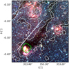 |
Fig. 1 Composite image of G353: IRAC 3.6 µm (in blue), 4.5 µm (green), and 5.8 µm (red). We indicate the ALMA-IMF N2H+ (1–0) coverage with a light green contour. We highlight ATLASGAL emission (870 µm) at 40 mJy beam−1 with the gray contour, corresponding roughly to a Herschel-derived N(H) of ~ 5.5 1022 cm−2. |
2 Data
2.1 ALMA-IMF data
We make use of the N2H+ (1–0) 12 m, 7 m, and Total Power observations described in Motte et al. (2022) for our analysis, providing robust uv plane coverage. We image the combination of the N2H+ 7m and 12m (from now on called “7m+12m”) measurement set of G353, using the publicly available imaging scripts from the ALMA-IMF github repository2. These data are corrected by the primary beam response pattern. Due to the missing large-scale emission, we find that near the VLSR of the protocluster (−17 km s−1; Wienen et al. 2015; Motte et al. 2022) some subregions in the 7m+12m cube present deep negative artifacts (“negative bowls”). To cover all possible uv scales, we combine the N2H+ 7m+12m continuum-subtracted cube with the Total Power observations from the ALMA-IMF LP. We use the feather3 task from CASA 5.6.0. With this combination, we were able to recover the missing flux, seen as negative bowls, present in the interferometric-only data. We produce a fully combined, multi-scale, feathered dataset which we use for our dense gas kinematic analysis.
To estimate and subtract the continuum emission present in the 7 m+12 m cube, we use the imcontsub4 CASA task. We select the emission-free channels between −43 km s−1 and −33 km s−1, and set the polynomial degree of the continuum fit (fitorder) to zero. We list relevant final image parameters in Table 1, such as the field size, pixel scale, beam size, root-mean-square noise (RMS), and channel width.
We use 12 m datacubes from Cunningham et al. (2023) to compare the shock tracers SiO (5–4) and CO (2–1) to our N2H+ kinematic analysis. We use DCN and N2H+ data to determine core velocities (Sect. 4.2). To determine total masses in specific regions we use the N(H2) map from Díaz-González et al. (2023).
Relevant parameters of the N2H+ 7m+l2m imaging.
2.2 Core properties from published catalogs
We use the cores catalog5 from Louvet et al. (2024). These cores were identified using the getsf algorithm, specialized in source extraction on regions with complex filamentary structures (Men’shchikov 2021). This procedure was done using the 1.3 mm continuum maps, smoothed at a common resolution of ~2700 au, obtaining a total of 45 sources for G353. We also use the DCN core velocities (15 sources, Cunningham et al. 2023) and the SiO outflow catalog (16 sources, Towner et al. 2024) in order to look for correlation between the N2H+ gas kinematics and cores/outflows position and properties. It is worth mentioning that, within a radius of 0.3 pc from the center of G353 (Motte et al. 2022), we find 60% of the 1.3 mm cores (27 sources), and ~ 70% of the cores with DCN velocities and SiO outflows (11 sources from each catalog). Of these 11 outflows, 7 are “red” 3 are “blue” (monopolar), and 1 is “bipolar” (Towner et al. 2024). The presence of these sources might imply a complex velocity field in this region, given that cores and outflows disturb the kinematics of the surrounding gas.
3 N2H+ isolated component analysis and filament extraction
The N2H+ (1–0) transition is characterized by its hyperfine emission composed by seven components (Caselli et al. 1995, see their Fig. 1). We present an ideal example of N2H+ emission in Fig. 2, panel d. In this work, we refer to the triplet of hyperfine components that present the highest intensities as the main N2H+ components, located at the center of the line emission at vrest = 93.173806 GHz. We refer to the most blueshifted hyperfine component as the isolated component, at νrest = 93.17631 GHz, shifted by ∼−8 km s−1 relative to the main N2H+ component (see Table 1 from Cazzoli et al. 1985).
3.1 Isolated component identification and extraction
We developed an algorithm to extract only the isolated hyper-fine component from every pixel in the feathered datacube. This is in order to reduce the complexity of our data, given that it may contain multiple velocity components in addition to the hyperfine line emission. Considering that the N2H+ emission moves in velocity across the protocluster, our approach is to find the velocity where the emission of the isolated component ends and remove the rest of the line emission. We also preserve the emission-free channels, at low (−43 km s−1 to −31.5 km s−1) and high (0.7 km s−1 to 6.7 km s−1) velocities, to improve future RMS estimations if needed. It should be noted that in the procedures described below, we use find_peaks6 to detect peaks and valleys in the different spectra.
Our extraction approach is separated into two procedures, for low and for high signal-to-noise ratio (S/N) data (see Fig. 3, and text below). In order to determine which data have low or high S/N, we obtained the mean spectrum over all the spatial pixels of the cube, which serves as a guide to determine the velocity at the “mean dip” (Vmean dip = −22 km s−1, dashed gray line in Fig. 2 panel “a”). This velocity represents the mean location of the intensity valley between the isolated and the main components of the N2H+ emission. We defined ΔVmean = 3.2km s−1 as the difference between Vmean dip and the velocity at the peak of the mean isolated component Vmean peak (dashed black line in Fig. 2 panel “a”), used in our velocity guesses for the high S/N extraction procedure (see below).
To create a S/N map of the isolated component, we first measured the RMS noise in emission-free channels (−43 km s−1 to −31.5 km s−1), and the peak intensity in the channels range in which the mean isolated component is located (−43 km s−1 to Vmean dip). This approach allows us to exclude the emission of the main line components. We encountered spurious emission at the edges of the S/N map. We adopted the procedure from Towner et al. (2024) by using the image processing techniques implemented by binary_erosion7 (1 iteration) and binary_propagation8 to clean the data for further analysis. binary_erosion allows us to remove the spurious emission in the outskirt of the map, although this approach also removes high S/N edges of our protocluster. Then, we used binary_propagation on the cleaned S/N map, using the original S/N map mask, to restore only the protocluster edges. To test our cleaning approach we computed the total integrated intensity using the Python package SpectralCube9 in the range of −31.5 km s−1 to Vmean dip using the original and cleaned S/N mask. We estimated that the removed spurious emission accounts for ~2% of the total integrated intensity for data with S /N > 5.
In Fig. 3, we show the N2H+ isolated component S/N map, where at S/N values ≥5 we capture the cloud emission while excluding noise (white contour). We set our isolated component S/N threshold to 5, in order to use one of the two extraction procedures (see below). In this section we refer to high (low) S/N spectrum if its isolated component S /N ≥ 5 (< 5). For low S/N spectra, we extracted all the channels in the velocity range from −43 km s−1 up until Vmean dip (panel “b” in Fig. 2). We take this approach given that for low S/N data we cannot identify peaks in the N2H+ emission in a reliable manner. For high S/N spectra the extraction procedure consists of creating different velocity guesses that represent the location of the intensity valley, similar to the definition of Vmean dip (Fig. 2). Then, we selected a velocity guess based on its associated weight (see description below). This approach is described in detail here:
First, we implemented a rolling average along each spectrum. This is in order to smooth over intensity bumps that might result in false positives for the detection of peaks and valleys. For this procedure, we averaged considering two channels before and after each velocity.
After smoothing, for each spectrum we identified the isolated component peak using find_peaks. We called the velocity associated with this peak Visolated component. In the case of multiple velocity components it represents the most blueshifted one. We found the intensity valley between the isolated component and the N2H+ main line emission by inverting the spectrum and finding the first peak which is the inverted intensity valley. We defined the associated velocity to this intensity valley as Vfirst minima.
We created three velocity guesses based on the properties of each spectrum in our cube (see points below). These are the 1st guess: Visolated component + ΔVmean.2nd guess: Vfirst minima in the case of multiple isolated components this guess might incorrectly capture the intensity valley after the first isolated component. In that case, the other guesses are needed for a reliable isolated component extraction. 3rd guess: Vmean dip + ΔVmean to provide a velocity cut further away from the V mean dip. This guess is mainly useful in the case where multiple isolated components cover a velocity range larger than the one probed by the other two guesses.
From each velocity guess we estimated two parameters to later decide which one to use. One is the absolute value of its associated intensity “Ii” (i.e., intensity at the guess velocity), and the other is distance in velocity “dVi” to the mean dip. The i subscript represents the guess associated with these parameters. We save the parameters of each guess in the lists “I” and “dV”.
-
We normalized these lists by their minimum value ensuring that the guess with the smallest “Ii” and “dVi” will have a weight (w) of 1, defined in Eq. (1). We do not encounter divergences in this normalization given these parameters are not exactly zero.
 (1)
(1)in which the “norm” subscript indicates that the parameter list is normalized by dividing it by its minimum value.
By visual inspection we considered that we obtain good extraction results when the weight is mostly dependent on dV and in a minor part on I. This is reflected by the 0.2 and 0.8 factors multiplying Inorm and dVnorm, respectively, in the definition of “w” in Eq. (1).
We chose the guess with the weight closest to unity.
Similarly as for S/N < 5, we extracted the spectra from −43 km s−1 up until the velocity of the chosen guess, and preserved the emission-free channels from 0.7 km s−1 to 6.7 km s−1.
Various examples of N2H+ spectra and isolated hyperfine component extraction are shown in Fig. 2, in which we can see spectra containing one (panel “c”), two (panel “e”), and three (panel “f”) velocity components, all well extracted by our procedure. In Stutz et al. (in prep) this approach is generalized to all ALMA-IMF regions for N2H+, providing reliable results.
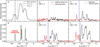 |
Fig. 2 N2H+ spectra involved in our isolated component extraction procedure. Panel a: normalized average N2H+ spectrum (solid black line) over the entire region. We show the location of the mean peak of the isolated component (dashed black line) and the “mean dip” (dashed gray line), see text. Middle and right panels: normalized example spectra (within a pixel) of the N2H+ isolated velocity component extraction procedure (see Sect. 3). We show G353 N2H+ spectra with solid black lines and the extracted isolated component, along with emission-free channels, with dashed red lines. Panel d: expected N2H+ emission for an excitation temperature of 15 K, an opacity of 1, velocity centroid of −17 km s−1, and a line width of 0.2 km s−1. We see the seven hyperfine components characteristic of this tracer, in which the most blueshifted corresponds to the isolated component. To derive this emission we use “n2hp_vtau” model from PySpecKit. In panels b, c, e, and f) we indicate Vmean dip with a dashed gray line. We present data with S /N < 5 in panel b, in which we make a rough extraction based on the Vmean dip. We show data with S /N ≥ 5 in panels c, e, and f, presenting clear single, double, and triple N2H+ isolated velocity components, respectively. In these examples we represent the selected velocity guess that separates the isolated component emission from the main line emission with dashed blue lines. The offset positions (Δl, Δb) of the spectra in panels b, c, e, and f are (0.68 pc, 0.27 pc), (0.12pc, −0.28 pc), (−0.08 pc, 0.47 pc), and (0.16pc, −0.07pc), respectively. These offsets are estimated relative to the center of the region (see Sect. 1). |
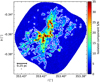 |
Fig. 3 G353 N2H+ isolated component S/N map. The white contour indicates the location of data with an isolated component S/N ≥ 5. We show the location of the 1.3 mm cores presented in Louvet et al. (2024) with black ellipses and are located in regions with S/N ≥ 15. We indicate the beam size of these data with a gray ellipse at the bottom left corner. Outside the S/N contour we make a rough extraction of the isolated component (see text). For data inside the S/N contours, we implement a procedure based on detection of peaks and valleys, to individually extract high (≥5) S/N isolated components (see Sect. 3). |
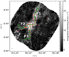 |
Fig. 4 Moment 0 map of the extracted N2H+ isolated component emission. We use the FilFinder Python package to identify the main filamentary structure present in G353 (see Appendix A). We identify three filaments (F1, F2, and F3; green lines) converging toward the central hub. The location of most of the 1.3 mm cores (red ellipses), projected in the POS, lie on top of the spine of these filaments, specially in the hub. |
3.2 Filamentary identification
We use the FilFinder Python package (Koch & Rosolowsky 2015) in order to detect the most prominent filaments in this region (green lines in Fig. 4). The procedure, including the parameters we used for the filamentary identification, is presented in Appendix A. In Fig. 4, we indicate the detected filaments with green lines, on top of the moment zero map of the multiple N2H+ isolated components. We see that G353 is a hub-filament system (HFS), composed by three main filaments converging at its center. The HFSs are a characteristic feature of early stages of star formation, in which gas flows through the filaments toward the central hub triggering star formation (Myers 2009; Galván-Madrid et al. 2010; Busquet et al. 2013; Galván-Madrid et al. 2013; Peretto et al. 2014; Kumar et al. 2022; Zhou et al. 2022). We see that in the plane of the sky (POS) most of the 1.3 mm cores (red ellipses) are located on top of the filaments. This spatial agreement between filaments and protostelar cores is consistent with filamentary fragmentation (André et al. 2010; Busquet et al. 2013; Stutz & Kainulainen 2015; Kuznetsova et al. 2015, 2018).
4 N2H+ isolated component velocity decomposition
In Fig. 2, we see that clear multiple isolated velocity components are present in our dataset. In this section we present our approach regarding the line modeling of these multiple velocity components. We also show how we use these models to determine core velocities.
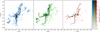 |
Fig. 5 Spatial distribution of the modeled N2H+ isolated velocity components. We indicate the main filament structure with green lines (see Fig. 4). In blue, green, and red we indicate the first, second, and third velocity components, respectively. We indicate the beam size of these data with a gray ellipse at the bottom left corner. The emission of the first and second components is more extended and intense than the third, most red-shifted velocity component. The 1.3 mm cores match regions with high integrated intensity, mostly traced by the first and second velocity components. |
4.1 Modeling of the isolated component emission
To characterize the complex dense-gas kinematics traced by N2H+ we followed the method in Álvarez-Gutiérrez et al. (2021), and we used the spectroscopic toolkit PySpecKit (Ginsburg & Mirocha 2011; Ginsburg et al. 2022) to model and decompose the isolated component emission. PySpecKit adjusts a fixed number of components set by the user, based on visual inspection of the data we imposed three velocity components to every spectrum and then remove false positives (see below). Given the kinematic complexity of the data and cursory inspection of the spectra, a simpler analysis with only two components contradicts the data. In essence, three components is the simplest possible choice, given the data. While this might fail for a small number of spectra that could require ≥ 4 velocity components, the residuals indicate that this could occur in a severe minority of cases, and hence more components is not warranted given the S/N and resolution of this particular dataset. To improve the convergence of PySpecKit, we created a set of ranges for the parameters that define each of the three Gaussian velocity components, namely the peak intensity, central velocity, and velocity dispersion. After testing different parameter ranges, we set the intensity range between 1.76 K (four times the mean RMS) and 30 K, the velocity centroid from −30 km s−1 to −20 km s−1, and the velocity dispersion from 0.22 km s-1 to 1 km s-1.
From the results using the ranges defined above, we notice that some modeled components do not fit any emission. These fits are the result of imposing to the fitter a fixed number of components, given these spectra can be better represented by one or two velocity components. In these fits there is no uncertainty estimation for both the peak intensity and velocity dispersion. Based on these two criteria we removed those velocity fits from the modeled cube. With this cleaning approach we are left with spectra characterized by one (~34%), two (~53%), and three (~13%) Gaussian velocity components. We present the Gaussian fits of the high S/N spectra from Fig. 2 in Appendix B.
In Fig. 5, we show the spatial distribution of the multiple Gaussian velocity components. In gray we indicate the main filamentary structure in the region (see Sect. 3.2). The first and second velocity components, in blue and green, respectively, present most of the high intensity emission and they also spatially dominate over the third, most red-shifted component. Both the first and second components trace mostly the filaments F1 and F3 from Fig. 4, where most of the 1.3 mm cores are located. The position of these cores coincide with high integrated intensity regions in these isolated velocity components. The most redshifted component is compact and less intense compared to the first and second velocity components. This velocity distribution is located mostly along the filament F2 and the central hub (see Fig. 4). In Fig. 6, we present the number of Gaussian velocity components for each spectrum, where we highlight that:
Most of the N2H+ data presents emission characterized by two velocity components.
Most of the spectra described by three velocity components are located in the innermost parts of the region.
Most of the cores (black ellipses; Louvet et al. 2024) are located in regions with spectra presenting two to three Gaussian velocity components, indicating kinematic complexity even at ~4 kau (N2H+ spatial resolution).
Single velocity component spectra are located preferentially in the outskirt of the protocluster.
In Fig. 7, we show the histogram of the fitted velocity centroid of each Gaussian velocity component. The peaks of these distributions are located at −27, −24.7, and −23.3 km s−1, respectively, well-separated in velocity. From hereafter we refer to these distribution as blue, green, and red, respectively. Most of the velocity components appear to be associated with the blue and green distributions. For consistency with the different tracers used in further analysis, we shift the isolated component velocities by +8 km s−1, to the reference frame of the main line components of N2H+ (Cazzoli et al. 1985).
4.2 DCN and N2H+ derived core velocities
In this section, our goal is to increase the sample of core velocities from the already published DCN catalog, aiming to explore all the potential in these types of dataset. Given the relatively high ncrit of DCN (3−2) (~ 107 cm−3) compared to N2H+ (1−0) (2 × 105 cm−3), DCN (3−2) is known to coincide well with continuum peaks associated with cores (Liu et al. 2015; Cunningham et al. 2016; Minh et al. 2018), while N2H+ is characterized by tracing the dense gas at the innermost parts of star-forming regions (Fernández-López et al. 2014; Hacar et al. 2018; González Lobos & Stutz 2019).
In Cunningham et al. (2023), they use ALMA-IMF 12 m observations of DCN (3−2) to study cores kinematics. They apply line emission fits for the DCN spectra inside the 1.3 mm cores from Louvet et al. (2024). For this procedure they determine core velocities in all ALMA-ΓMF targets. They classify as DCN single and complex core velocities, spectra that can be fitted with one or multiple Gaussian velocity components, respectively. Due to a global conservative S/N threshold the DCN fitting process missed the velocity estimation of some cores. For G353 only 15 out of the 45 cores present DCN velocity fits.
We used the ALMA-IMF DCN 12 m data from Cunningham et al. (2023), which presents a velocity resolution of ~0.34 km s−1. For each DCN core velocity described by a single component (Cunningham et al. 2023) we compared the emission of the DCN and modeled N2H+ isolated spectra. We found an average velocity offset between the DCN peak and the closest N2H+ isolated component peak of ~0.65 km s−1, less than two DCN channel widths. We used this approach for the remaining 30 cores, in order to determine their DCN velocities.
Here we estimated the RMS of the DCN data in emission-free channels in the range of −42 km s−1 to −25 km s−1 and we obtain the S/N map by dividing the peak intensity by the RMS. For the procedure below we only used DCN spectra with S/N > 3. Next, we extracted the average DCN and modeled N2H+ isolated component spectrum of these 30 cores. We identified the N2H+ isolated velocity component closest to the DCN peak within three DCN channel widths. We found that 11 out of these 30 cores present DCN with S/N> 3 close to one N2H+ velocity component. Here, we defined the velocity of these cores as the velocity where the DCN emission peaks. On average, these cores have a velocity offset between these two tracers less than 0.8 km s−1 (<2.5 DCN channels), similar to the results obtained for the 15 cores with DCN velocities from Cunningham et al. (2023), and they present an average velocity offset of 0.38 km s−1. Throughout this paper we refer to these cores as “DCN & N2H+ cores” given they are derived from the comparison of these two tracers. In Appendix C we present two examples of the comparison of the DCN and N2H+ spectra in cores in which we see clear agreement between these tracers (Fig. C.1). In Table C.1 we show these obtained core velocities from our comparison between DCN & N2H+ spectra, complementing the DCN catalog from Cunningham et al. (2023).
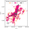 |
Fig. 6 Spatial distribution of the modeled N2H+ isolated component spectra. These models are composed by up to three Gaussian velocity components. The 1.3 mm cores and beam size are the same as in Fig. 3. Most of the 1.3 mm cores are located in regions with spectra presenting two to three velocity components (see Sect. 4.1). |
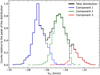 |
Fig. 7 Normalized velocity centroid distributions of each N2H+ Gaussian velocity component. The velocities at the peak of the distributions are −26.9 km s−1, −24.7 km s−1, and −23.3 km s−1 for component 1 (blue), 2 (green), and 3 (red), respectively (see Sect. 4.1). |
5 Analysis of position-velocity diagrams
5.1 Traditional position-velocity diagram
We start by analyzing the “traditional” PV diagram shown in Fig. 8. We created this diagram by taking the total intensity along the Galactic longitude, in which Δb indicates the distance in parsec relative to the center of G353, assuming a distance to the protocluster of 2 kpc (Motte et al. 2022). We see general agreement between the DCN core velocities and the N2H+ velocity distribution. This suggests that most of the cores are still kine-matically coupled to the dense gas in which they formed. As is presented in Sect. 4.2, the DCN and N2H+ velocities match within 0.8 km s−1 (<2.5 DCN channels).
Regarding the dense gas velocity distribution, in Fig. 8 we see a velocity spread of ~8 km s−1 in the subregion between Δb ~ −0.3 pc to 0.1 pc. Most of the intensity on this diagram is located at the upper part of this subregion, at Δb ± 0.1 pc. This spread is also present in the PV diagram along Δb and Δl shown in the top right and bottom left panel of Fig. 9. We explore the possible origin of this structure in Sect. 6.
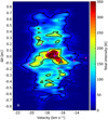 |
Fig. 8 “Traditional” PV diagram of the N2H+ modeled isolated components, created by collapsing the l coordinate. Δb indicates the distance along b in pc, relative to the center of G353, assuming a distance of 2 kpc (Motte et al. 2022). The colormap indicates the total intensity along l. With fuchsia and black crosses we show the 1.3 mm cores with single and complex DCN velocities detections, respectively (Cunningham et al. 2023). With dark cyan “×” markers we show the 1.3 mm cores with velocities derived from DCN and N2H+ data (see Sect. 4.2). The size of the markers indicate relative mass (Louvet et al. 2024). Black contours indicate total intensities at 40, 160, 280, and 400 K. We see a large-scale velocity spread (ΔV ~ 8 km s−1) around Δb ~ −0.3 pc − 0.13 pc (see also Sect. 5.2). We show the major axis of the beam and the channel width with a white rectangle at the bottom left corner. |
5.2 Intensity-weighted PV diagrams
In the top left panel of Fig. 9 we show the spatial distribution of the fitted Gaussian velocity components (see Sect. 4.1). The blue, green, and red color maps indicate the integrated intensity of the first, second, and third velocity components of the N2H+ spectra, respectively. We note that the spatial overlap between any of these components is presented in Fig. 6.
As is seen in Fig. 8, the traditional PV diagram provides information on the dynamics on the large, protocluster-scale, environment. Meanwhile, the intensity-weighted PV diagram (Fig. 9), in which the color of each point indicates its integrated intensity, highlights the small core-scale kinematics. Similarly as in González Lobos & Stutz (2019) and Álvarez-Gutiérrez et al. (2021), from the isolated component line decomposition (Sect. 4.1), we derived the integrated intensity and velocity centroid for each Gaussian velocity component. Using these parameters we created intensity-weighted PV diagrams along the b and l coordinates. We present these N2H+ PV diagrams in the bottom left and top right panels of Fig. 9. The key features on the position-position (PP) and on the top right PV diagram, are:
The agreement between the DCN core velocities and the overall N2H+ PV structures suggests that cores are still kinematically coupled to the dense gas in which they formed.
We see at least nine clear and prominent V-shaped velocity gradients (see Appendix D), across all velocity components. The orientation of these V-shape, pointing to the left/right (top right panel) or up/down (bottom left panel), follow no clear preference.
In some cases, the vertex of these V-shapes is close spatially and in velocity to the location of cores.
In the plane of the sky (POS), all three velocity components overlap in most of the region.
This technique recovers the large-scale velocity spread present in Fig. 8 and highlights small-scale structures.
The most prominent V-shape is located at (Δb, V) = (−0.14 pc, −20.5 km s−1), between two 1.3 mm cores with DCN detections (see Sect. 6).
For a better visualization of the 3D structure of these V-shapes we provide an interactive 3D PPV diagram online.
5.3 Velocity gradients
In this section, we focus on the most prominent blue V-shape (Fig. 9, top right panel). In Fig. 10, we show this velocity distribution, named V-shape “C”, in detail. Given the visual linearity of the VGs composing the V-shape, we applied a linear fit to these distributions in order to characterize them. For these fits we considered data only above an integrated intensity threshold of 8 K km s−1 and 3 K km s−1, for the upper and lower gradient, respectively. We removed data not related with the VG, clustered in the ranges of (Δb, V) ~ (−0.025 − 0.04pc , −19.5 − −18.5 km s−1), which lie just outside the filament hosting this V-shape on the POS. Additionally, we weighted each point based on their integrated intensity to make our fits more robust. The slopes of the linear fits represent the VGs in km s−1 pc−1. These linear fits follow the VGs distribution and these are somewhat asymmetric, the upper gradient is slightly shallower than the bottom gradient. Given the unknown inclination angle (θ) of these structures relative to the POS, the observed VG is just a fraction of the original VG. These are related as VG = VGoriginal ⋅ sin(θ). These VGs present values between ~13 to ~ 18 km s−1 pc−1 (see Fig. 10). Additionally, we estimated the center of this V-shape as the velocity-weighted mean position of the points composing this structure. With this approach the position of the points closest to the V-shape apex present more weight, obtaining the center of this V-shape at (l, b) = (353.4135°, −0.3657°). This position is located between “core 2” and “core 3”, both of them having DCN velocity fits (Cunningham et al. 2023). These cores present masses of 20.7 and 9.4 M⊙, respectively. We inspected the core catalog from Louvet et al. (2024) and concluded that the location of this V-shape do not coincide with any core.
In the left panel of Fig. 11, we show the integrated intensity of the multiple modeled N2H+ isolated components. With colored boxes we show the areas where we create the different PV diagrams presented on the right panel. These boxes are centered at the main blue V-shape, matching the area of this V-shaped structure (see Fig. 12). We show that the overall structure in PV space is conserved at different angles, excluding the possibility of this velocity feature being the result of projection effects.
For this V-shape we used its composing VGs to derive timescales as tVG = 1/VG, similar to the procedure for a rotating filament presented in Álvarez-Gutiérrez et al. (2021), and we suggest these can be interpreted as inflow timescales. The tVG values for this V-shape range between ~ 50–70 kyr. These timescales are short compared to the ~0.21 Myr free fall time (tff) of the protocluster (Motte et al. 2022), and a few times larger than the tff of nearby cores (~20 kyr, within 0.1 pc of this V-shape). To determine the cores tff, we use the 1.3 mm core masses from Louvet et al. (2024).
We characterized eight more N2H+ V-shaped structures. In Fig. 13, we show the position of these V-shapes in the POS. Previous studies have detected VGs along filaments, toward a converging point (Peretto et al. 2014; Pan et al. 2024; Rawat et al. 2024). In the case of G353 we see that instead of detecting a single V-shape at the intersection of its filaments, the hub appears to be fragmented into multiple, small-scale V-shaped VGs. Only V-shapes “A”, “D”, and “E” are outside of the hub, with V-shape “D” located on top of filament “F3”. This indicates that the V-shaped structures are not exclusive to the central parts of HFS, but are also present in comparatively isolated regions. We note that within a ~beam size from the apex of V-shape “B” (see Fig. D.2), the continuum core “7” (~6 M⊙) is located.
In Henshaw et al. (2014), they propose two scenarios that might produce these V-shaped VGs (see their Fig. 12). One scenario suggests that gas in a filament is flowing toward a denser region (infall), while the other scenario suggests that a protostellar outflow moves the dense gas located in its vicinity. To analyze the different dynamical processes present in this region, we used the ALMA-IMF 12 m data of the shock, outflow tracer SiO (5–4), from Cunningham et al. (2023). From those data we created its intensity-weighted PV diagram, presented in Fig. E.1 (see Appendix E for more details). We note that there is almost no SiO emission nor outflow sources at the location of the N2H+ V-shape (see Fig. 12). The ∆V within 10″ from this main blue V-shape is ~40 km s−1, while for the whole SiO dataset is ~80km s−1, showing a clear difference in the SiO ∆V and the core velocities. Furthermore, the SiO ∆V is ~ 10 times larger than the one of N2H+. This difference in traced velocities implies that these two molecules trace vastly different physical phenomena. We suggest that the small velocity range probed by N2H+ indicates that the VGs can be considered as infall signatures (see Sect. 6). We discuss the possible morphology of the filaments hosting V-shapes in Sect. 8.
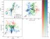 |
Fig. 9 N2H+ intensity-weighted position-position and PV diagrams of G353. Top left: spatial distribution of the fitted N2H+ Gaussian isolated velocity components (blue, green, and red, see Sect. 4.1). Ellipses indicate the location of the 1.3 mm continuum cores (Louvet et al. 2024). Orange indicates cores with no DCN detections. Fuchsia and black represent cores with single and complex DCN velocities (Cunningham et al. 2023). DCN & N2H+ cores are indicated with cyan. We show the beam size with a gray ellipse in the bottom left corner. Top right and bottom left: intensity-weighted PV diagrams along the b and l coordinates, respectively. For the 1.3 mm core velocities we use the same colors and markers convention from Fig. 8. For reference we indicate with a red arrow, in both the top right and bottom left panels, a VG of 10 km s−1 pc−1 corresponding to a timescale of ~0.1 Myr. We see multiple V-shapes near the location of cores across all velocities in the PV diagrams, more prominently in the top right panel (see Fig. D.1). The most prominent V-shape is located in the blue component, at (V, ∆b) ~ (−20.5km s−1, −0.14 pc) (see Sect. 5.2). We provide an interactive 3D PPV diagram online. |
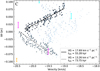 |
Fig. 10 Zoomed-in version of the top right panel of Fig. 9, centered at the prominent blue V-shape (“C”) located at (∆b, V) = (−0.14pc, −20.5 km s−1). We indicate the major axis of the cores with vertical lines in fuchsia (DCN single) and cyan (N2H+), similarly we represent the major axis of the beam with a vertical orange line. We apply linear fits to the upper and lower distributions, represented by darker points. These points are selected based on an integrated intensity threshold (see Sect. 5.3). We weight each point by their integrated intensity and derive VGs from the slope of these linear fits. The range of the obtained VGs is ~13 – 18 km s−1 pc−1. We defined the timescale associated with the VG as tVG = VG−1, being in the range of ~50–70 kyr. We show eight more well characterized V-shapes in Appendix D. |
6 G353 as a collapsing region
We used the SiO (5–4) and CO (2–1) data from Towner et al. (2024) and Cunningham et al. (2023) to identify possible outflows near the V-shape presented in Fig. 10. For CO we measured the RMS in the emission-free velocity range of 145–286 km s−1. We used only CO data with S /N > 3 for our analysis. The cleaning of the SiO data is described in Appendix E. In Fig. 12, with a fuchsia “×” we indicate the center of the V-shape from Sect. 5.3, located between two 1.3 mm cores 2 and 3 (black ellipses), which present DCN velocity detections. From these diagrams we see there is neither SiO nor CO outflow detection at the location of the main blue V-shape (∆l, ∆b) = (0pc, 0pc). In the right panel we show the position of the data composing this V-shape, where the velocity peaks toward the center of this velocity feature.
We derived the mass-weighted mean position of the two cores (2 and 3) closest to the V-shape to determine their barycen-ter (yellow “×” in Fig. 12). We found that the difference between the center of the V-shape and the barycenter of these cores is ~0.3″(~600 au), well below the beam size of the N2H+ data. A similar offset is also present in the intensity and velocity profiles along filaments from ATOMS data (Zhou et al. 2022, see their Fig. 6). This small spatial offset might suggest that the gas flowing in the V-shape is produced by the gravitational pull toward the barycenter of cores 2 & 3, where the N2H+ radial velocities peak. This interpretation is similar to the one proposed in Zhou et al. (2023) in their kinematic analysis of the G333 complex. They describe the V-shaped VGs as the result of gas funneling from the molecular cloud to clumps which is then funneled onto cores (see their Fig. 9) consistent with gravitational acceleration.
In Fig. 14, we show the mean spectrum of different tracers at the central position of the main blue V-shape. These spectra were measured over a circular region with diameter equal to the major axis of the N2H+ beam (2.28″; ~0.02 pc). This circular area results in a coverage of 1.14 times the N2H+ beam, and ~5.6 times the beams of the H2CO, DCN, and H213CO data. We see N2H+ and H2CO present double component spectrum with asymmetric peaks. Between these peaks we detect DCN and H213CO emission. The asymmetric spectrum present in N2H+ and H2CO is consistent with the “blue asymmetry” spectral feature, usually interpreted as infall signature, suggesting that this region is under gravitational collapse (e.g., Anglada et al. 1987; Mardones et al. 1997; Lee et al. 1999, 2001; Smith et al. 2012). Based on the idea that the V-shapes are the result of flowing gas along filaments toward denser regions, the blue-asymmetry detected at the center of the main blue V-shape suggests that gravitational collapse is taking place at the apex of the V-shaped structure.
Regarding large scales, in the traditional PV diagram presented in Sect. 5.1 (see Fig. 8), we see a clear velocity spread around ∆b ~−0.1 pc, also present in the top right panel of Fig. 9. Below we compare this velocity spread with the velocity distribution produced by infall, in which the gas velocities increase as the distance to the center of infall (“r”) decreases:
 (2)
(2)
For this comparison, we modeled a sphere with a total mass of 150 M⊙, a radius of 0.5 pc, and a power law density profile described by:
 (3)
(3)
We provide the derivation of ρ(r) in Appendix F. γ = 5.65 was determined by visual inspection by comparing the obtained radial velocities of the model (see below), at different γ values, with the overall shape of the PV distribution.
We then estimated the infall velocity of each point, based on the cumulative mass distribution (“M”) at any given distance to the center (Eq. (2)). We obtain the radial component of the infalling velocities as:
 (4)
(4)
in which X represents the horizontal coordinate in the POS, while Z represents the (unobserved) depth of the sphere. The spatial coordinates for this model range from −0.5 pc to 0.5 pc.
In Fig. 15, we show the coverage of the PV distribution from our model, described in Eqs. (2)–(4), with a solid white line. We find good agreement between the PV distributions of our approach and the data. The PV distribution of our infall model is consistent with previous work that provide the expected PV distributions for spherical protostellar envelopes under infall (Tobin et al. 2012). At large scales, we interpret the agreement between the PV diagrams of our model and the data as proto-cluster scale collapse due to gravitational contraction. It is worth noting that the inferred mass from our model is ~5.5 times lower than the one derived from the N(H2) map (Díaz-González et al. 2023). We speculate that a model considering complex processes such as turbulence, radiative transfer, and magnetic fields might solve this mass discrepancy while still matching the observed PV distribution.
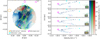 |
Fig. 11 Left panel: integrated intensity map of the modeled N2H+ isolated component within a region of radius of 0.1 pc, centered at V-shape “C”. With boxes in shades of green and yellow, we indicate the different paths taken to create the PV diagrams shown on the right panel. The area covered by these four PVs matches the extent of this V-shape (see Fig. 12). The 1.3 mm cores are indicated using the same convention from Fig. 9. For the cores within the radius of 0.1 pc we indicate their IDs in black. Right panel: PV diagrams associated with the colored rectangles in the left panel. At the bottom right corner of each sub panel, with colored values, we indicate the angle (counter-clockwise) of each PV path. The PV paths match the V-shape coverage (right panel of Fig. 12). We see the overall structure of this V-shape persists at different angles, indicating that these structures are not a result of projection in the POS. |
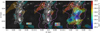 |
Fig. 12 Multi-tracer diagram at the location of the main blue V-shape of G353 (Sect. 5.3). The different panels show the step by step construction of the final plot (right panel). Left panel: the black to white background shows the 1.3 mm continuum emission from Díaz-González et al. (2023). With black ellipses we show the 1.3 mm continuum cores from Louvet et al. (2024). With black text we indicate the IDs of the cores closest to the center of the V-shape, marked with a fuchsia “×”. We indicate the barycenter of cores 2 & 3 (see Fig. 11) with a yellow “×”. Filled contours represent the CO (2–1) emission in the velocity ranges of −50 km s−1 to −15 km s−1 (cyan) and 15 km s−1 to 50 km s−1 (beige), relative to the Vlsr = −17 km s−1 of G353. With a white contour we indicate the log (N(H2) cm2) = 23.3. Middle panel: in addition to the left panel, we include the SiO (5–4) emission with blue and red contours in the same (negative and positive) velocity range as with CO. The pink contour indicates the integrated intensity of the most blueshifted modeled N2H+ Gaussian velocity component (see Fig. 9; blue distribution), at a value of 7 K km s−1. Right panel: with open circles we show the location of the data composing the main N2H+ blue V-shape. The colors indicate their velocity centroid, and their (increasing) size indicates how close the gas velocities are to the velocity apex of the V-shape. This VG seems to converge to the barycenter of cores 2 and 3, and it is oriented along filament “F3”. |
7 Mass accretion rates in the V-shaped structure
Based on the idea that the V-shapes are a result of gas flowing toward cores, in this section we provide estimates of their mass accretion rates (Ṁin) for N2H+ and H2.
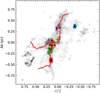 |
Fig. 13 V-shapes location on the plane of the sky. We indicate the position of each V-shape with colored points and their ID with black text. With red lines we show the filamentary structure identified in Sect. 3.2. In the background we show the integrated intensity map of all three velocity components, similarly as in Fig. 9. We see most of the V-shapes are located at the hub. |
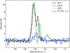 |
Fig. 14 Mean spectra within a 1.14″ (~0.01 pc) radius around the location of the main blue V-shape (pink “×” in Fig. 12). Both N2H+ and H2CO show blue asymmetry, known to characterize infall motions. The difference in velocity between the two N2H+ peaks is ~2.5 km s−1. |
7.1 H2 mass accretion rate
Here we describe our approach for V-shape “C”, and to ensure that we estimate the V-shape M(H2) on the area of this structure, we used the CASA task imregrid to obtain the continuum-derived N(H2) map from Díaz-González et al. (2023) at the resolution of the N2H+ data. We determined that in this V-shape the total N(H2) ~ 1.17 × 1026 cm−2 in an area of 0.013 pc2. Here, we derived a M(H2) map using Eq. (5):
 (5)
(5)
from this M(H2) map we considered only the points that are part of the V-shape. To determine the mass associated with flowing motions we subtracted the core masses (from Louvet et al. 2024) that are located inside this V-shape. We note here that this mass map is an upper limit given that we do not apply a background correction. We obtained a total of M(H2) ~ 53 M⊙. Considering tVG mean used in Eq. (8), we derived the Ṁin (H2) as:
 (6)
(6)
We used the procedure described above to estimate the Ṁin (H2) of the other eight V-shapes shown in Fig. D.2. We include these values in Table D.1. The average Ṁin (H2) of these V-shapes is 3.4 × 10⁻⁴ M⊙ yr−1. We note that V-shapes “H”, “C”, “F”, and “B” present the largest Ṁin (H2) and they are located near or at the convergence point of the filaments (see Fig. 13).
For comparison, using the core masses from Louvet et al. (2024) we estimate the free-fall time of all 45 1.3 mm cores and their mass accretion rates. These values present large scattering, ranging from (0.07–25) × 10−4 M⊙ yr−1, with 28 of these cores presenting Ṁin (H2) < 10−4 M⊙ yr−1. For cores 2 & 3, the average Ṁin (H2) is 15.5 × 10⁻⁴ M⊙ yr−1, about twice the Ṁin (H2) of the main blue V-shape, located between these two cores.
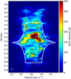 |
Fig. 15 PV coverage of a gravitationally collapsing sphere. The white contour represents the coverage of the synthetic radial velocities derived from this model (Sect. 6). The background and cores are the same as in Fig. 8. For the modeled sphere we set its total mass to 150 M⊙, within a radius of 0.5 pc. |
7.2 N2H+ mass accretion rate and relative abundance
To derive the N2H+ Ṁin associated with the main blue V-shape (Fig. 10), we need to estimate its N2H+ mass. For this procedure we used PySpecKit with the n2hp_vtau fitter, to fit the full N2H+ line. The fitted parameters (see below) allow us to derive the N(N2H+). The V-shape structure contains 77,143, and 25 N2H+ spectra with one, two, and three velocity components, respectively. The bluest velocities in the three velocity component spectra accounts for ~2% of the total number of velocities in this V-shape. For this reason, we modeled the full N2H+ hyper-fine line structure with one and two velocity components. In Table 2 we list the parameters and ranges used for this procedure.
After obtaining the modeled N2H+ cube, we removed modeled components that presented τRMS/τ > 0.3, in which τ and τRMS represent the estimated opacity and its associated error, respectively. This criterion is to ensure that we use reliable fitted parameters to determine our N(N2H+) values. For the fitting of two N2H+ components we only analyzed the most blueshifted component. The resulting opacities follow a log-normal distribution with a peak at τ = 0.13.
We derived the N(N2H+) of the V-shape by using Eq. (7) (Caselli et al. 2002b):
 (7)
(7)
in which τ, Tex, and ∆v are the opacity, excitation temperature, and velocity dispersion, respectively, obtained from the full line fitting. The Planck and Boltzmann constants are represented by h and k, respectively, v and λ are the frequency and wavelength of N2H+, A is the Einstein coefficient of the N2H+ (1–0) transition, 𝑔l and 𝑔u are the statistical weights of the lower and upper energy levels, El is the energy of the lower level, Qroι is the partition function estimated using the excitation temperature of the full N2H+ fits (see Eq. (A2) from Caselli et al. 2002b).
From the above procedure, inside the V-shaped structure, we get a total N(N2H+) = 5.24 × 1015 cm−2 and a total M(N2H+) = 5.9 × 10⁻⁸ MQ, within its extent of 0.013 pc2. We used the average timescale of the VGs from Sect. 5.3 (Fig. 10), tVG mean = 64.5 kyr, to determine the Ṁin (N2H+) as:
 (8)
(8)
The Ṁin (N2H+) estimate (and Ṁin (H2) below) should be multiplied by sin(θ), in order to account for the unknown inclination angle (θ) of the protocluster/filaments relative to the POS.
For the main blue V-shape (Fig. 10), we derived the N2H+ relative abundance X(N2H+), using the N2H+ and H2 column densities obtained above, as:
 (9)
(9)
The X(N2H+) value obtained above appears lower than typical estimates in massive Galactic star-forming regions reported in different works ([1.6–3.8] × 10−10; Caselli et al. 2002a; Henshaw et al. 2014, Sandoval-Garrido et al. in prep.). We consider it a good agreement taking into account the uncertainties of the involved measurements (i.e., column density estimates). For a comparison of the N2H+ relative abundance between regions composing the V-shapes and the rest of protocluster we would require to model the full N2H+ line emission in the whole region.
N2H+ full line fitting parameter ranges.
8 Discussion
8.1 V-shaped velocity gradients in the literature
The V-shaped VGs described in this work have been detected across multiple Galactic star-forming system. Stutz & Gould (2016) introduced the Slingshot mechanism in the Integral Shaped Filament (ISF) located in Orion A. They show undulations of the region in both position and velocity, suggesting that these features appear to be ejecting protostars (see their Fig. 2). Furthermore, Stutz (2018) characterize a standing wave in the neighborhood of the ISF, consistent with the Slingshot mechanism. It is possible that the undulations in the works above might result in the observed V-shaped structures seen in different studies (see below). González Lobos & Stutz (2019) identify six evenly spaced (every ~0.44 pc) velocity peaks along the spine of the ISF in Orion A. They suggest that this periodicity is consistent with the wave-like perturbation in the gas caused by the Slingshot mechanism. In Álvarez-Gutiérrez et al. (2021) they analyze the L1482 filament located in the California Molecular Cloud. In all of the analyzed tracers there is a clear velocity peak in their north region (length ~1.8 pc, mass ~103 M⊙). This sub-region contains a higher gas density and higher number of YSOs compared to the more quiescent south part.
While the two regions described above are considered nearby (both at D ≲ 500 pc), more distant regions also present these velocity features which we list below. Zhou et al. (2022) study the velocity profiles along filaments from the ATOMS survey (Liu et al. 2020). The median mass of their sources is ~1.4 × 10³ M⊙ with a median length of the filaments at -1.35 pc. By analyzing the H13CO+ (1–0) emission they find converging VGs along filaments (see their Figs. 6 and 10), which they also detected using simulations from Gómez & Vázquez-Semadeni (2014). These VGs at scales comparables to the V-shapes presented here are consistent with our VGs estimates (see their Figs. 7 and 8). In Zhou et al. (2023) they analyzed 13CO (2−1) APEX/LAsMA data of the G333 complex. They identify multiple V-shaped VG (see their Fig. 7) which they describe as the PV projection of a funneling structure in PPV space (see their Fig. 9). The origin of this structure is due to material inflowing toward the central hub and also due to gravitational contraction of star-forming clouds or clumps.
Redaelli et al. (2022) use ALMA N2H+ (1−0) isolated component data of the high-mass (5200 M⊙) clump AGAL014.492-00.139 identifying multiple coherent structures in PPV space (trees “B” and “G”; right panel of their Figs. 7 and 9). These are characterized by multiple undulations, and possible V-shaped VGs. For their “G” PV distribution, they suggest that one scenario is where the dense gas is flowing along the filament (of length -0.2 pc) from protostar “p3” toward the protostar “p2”. This motion has an Ṁin =2.2 × 10⁻⁴ M⊙ yr−1, being in the range of the Ṁin we derive for our VGs (see Table D.1).
In Rawat et al. (2024) they analyze 13CO(1−0) data obtained with the Purple Mountain Observatory, as part of the Milky Way Imaging Scroll Painting survey. They detect a V-shaped VG (see their Fig. 14) along the ridge of the G148.24+00.41 (G148) cloud. This V-shape peaks toward the dense clump at the center of this region, possibly indicating gas inflow along their filaments F2 and F6 toward the hub. The length of the V-shape in G148 is ~15 pc, while our most prominent V-shape (Fig. 10) is ~0.2 pc. Also the masses and lengths of their identified filaments are (1.3 to 6.9) × 103 M⊙ and 14 to 38 pc, respectively, large compared to the total mass (2.5 × 10³ M⊙) and extent of G353 (~1.2 pc). This difference in probed lengths and masses might be reflected by their mean VG ~0.05 km s−1 pc−1, ~2.5 orders of magnitude smaller than our VGs. This is consistent with the analysis presented in Zhou et al. (2022, 2023), in which they observe an inverse relation between the spatial scale of a region and their VGs (see their Fig. 8).
In Pan et al. (2024) using APEX C18O (2−1) data of the filamentary cloud G034.43+00.24 (G34) they identify converging VGs of lengths ~1 pc toward the “middle ridge” (see their Fig. 3, top panel). They interpret these VG as gas flowing from the filaments onto dense clumps, located at the center of G34. These VGs of their southern and northern filaments are in the range of ~0.3–0.4 km s−1 pc−1, and they estimate the total mass inflow rate toward the middle ridge as ~5.5 × 10⁻⁴ M⊙ yr−1, similar to our M⊙ estimates.
Current work by Sandoval-Garrido et al. (in prep.) in G351.77 (intermediate protocluster, located at 2 kpc; Motte et al. 2022; Reyes-Reyes et al. 2024) use a similar analysis as we present in this work, in which they identify multiple V-shaped velocity structures. In Salinas et al. (in prep) they analyze the kinematics of the evolved protocluster g012.80 (located at 2.4 kpc; Motte et al. 2022), in which they implement similar techniques and find velocity signatures of filamentary rotation.
8.2 Filamentary 3D morphology
V-shaped VGs appear to be a generic feature across a wide range of star-forming environments, probing VGs with differences of up to ~2 orders of magnitude in spatial scales ranging from 0.1 to ~ 10 pc. Despite being commonly detected in recent studies, it is still not clear how they are produced. Henshaw et al. (2014) highlights the degeneracy regarding the opposite interpretations of these V-shaped velocity structures. They suggest that these VGs can be a signature of gas flows along kinked filaments toward a core located at their convergence point. From our analysis regarding the most prominent V-shape (see Sects. 5.3 and 6) we see that no core is located at its apex, although cores 2 and 3 are within -0.05 pc. Also the spatial offset between the center of the V-shape with the barycenter between these two cores is -600 au. This is consistent with the idea of small-scale gravitational collapse within the protocluster, similar to clump decoupling from their parent molecular cloud (Peretto et al. 2023). Based on this, we conclude that cores may be located in the vicinity of the velocity apex, and not necessarily on top of it. This gas flows toward denser regions may result in the formation of high-mass cores in later stages during the evolution of the protocluster.
Regarding the kinked morphology of the regions hosting V-shapes, one scenario regarding magnetized shocks is presented in Inoue & Fukui (2013) and Inoue et al. (2018). They use mag-netohydrodynamics simulations to characterize the interaction of molecular clouds and a magnetized shock produced by a cloud-cloud collision. They find that the shock layer decelerates as it collides with denser regions. This deceleration reshapes the shock layer to be oblique, leading to the formation of kinked filaments and converging flows, which are oriented toward the apex of these filaments. They predict that magnetic fields present in the region should be perpendicular to these filaments and bend with the shock around the filament (Inoue et al. 2018, see their Fig. 3). In Bonne et al. (2020) and Bonne et al. (2023) they propose that this scenario takes place in the Musca and the DR21 filaments. In both of these regions they detect V-shaped VGs which they suggest are the result of cloud-cloud collisions bending the magnetic field (Bonne et al. 2020, see their Figs. 22 and 23). Further observations of magnetic field polarization in the POS, along with information along the line of sight is required to evaluate these models.
Another possibility is that these kinked structures could be caused by mechanisms such as the Slingshot. This mechanism proposes a standing wave, longitudinal gravitational instabilities, or large-scale oscillations possibly caused by a possibly helical magnetic field morphology, causing ejections of protostars and protoclusters from their maternal filament (Stutz & Gould 2016; Stutz 2018; Stutz et al. 2018; Liu et al. 2019).
A different interpretation is that they are the product of outflowing material coming from a forming protostar interacting with the surrounding dense gas (see their Fig. 12). To shed light into this degeneracy in G353 we compare the N2H+ (dense gas tracer) radial velocities and SiO (shock/outflow tracer) as a proxy for energies. The velocity range ∆V covered by the N2H+ emission is ~8km s−1, while for SiO is ~80 km s−1. Given the difference in probed velocities between SiO and N2H+ (see Sect. 5.3) and the analysis presented in Sect. 6 we suggest that the V-shapes in G353 are a signature of infall.
The multiple VGs that conform the V-shapes present in G353 have values of ~8 to ~31 km s−1 pc−1, with timescales ranging from ~35–173 kyr, and Ṁin values (~0.4–9) × 10−4 M⊙ yr−1. These values are similar to VGs in other regions with comparable sizes and masses. In G353 it is likely that these VGs are the result of dense gas moving through filaments, possibly increasing the density of the central regions, shaping the overall velocity field at large and small scales, and leading to a further increase in the core population and star formation activity.
8.3 Timescales and mass accretion rates
One important aspect of the V-shapes that is still not well understood is the timescale associated with the VGs (tVG = VG−1). It is not clear if nor how these timescales determine core formation lifetimes or impact the star formation environment in general. In our sample of V-shapes the timescales are in tens of kyrs with the average value of ~67 kyr, ~ two times the cores tff, while the tff of the whole protocluster is ~0.21 Myr. In Rawat et al. (2024) they estimate the longitudinal collapse timescales for their filaments, being in the range of 5–15 Myr. Using their derived VGs we estimate their associated timescales to be between ~16 and ~50 Myr, ~ one to two orders of magnitude larger than our small-scale V-shapes timescales. We suggest that the VG timescales might serve as an upper limit for filamentary collapse timescales. In Zhou et al. (2022) they determine gas accretion times as a function of the lengths of their filaments, assuming that the VGs produced by gas inflow (see their Fig. 11). At filament lengths comparable to our V-shapes (~0.1 pc) their gas accretion timescales are on the order of our estimates (see Table D.1).
8.4 Depletion timescales
It is also interesting to consider the mass accretion rates measured here compared to the available protoclustermass reservoir to explore implications for the duration of the gas dominated phase. The total mass accretion rate of our V-shaped structures is Ṁin, Tot = 3 × 10⁻³ M⊙ yr−1 (see Table D.1). Considering the total mass (MTot) of G353 as a mass reservoir, we estimated the depletion timescale (tdep) as the time needed to fully consume the gas. Here we assumed that Ṁin, Tot is representative of flows feeding gas onto cores. We estimated tdep = MTot/Ṁin, Tot, in which the total mass of the region is 2500 M⊙ (Motte et al. 2022). We obtained a tdep = 0.8 Myr, of similar magnitude but about four times larger than the tff of the protocluster. Considering that our estimate of Min, Tot is certainly a lower limit (see discussion above), the actual value value of tdep is likely to be shorter, so closer to the free-fall time estimate. Given that the protocluster does not appear to be in a state of free-fall (see Sect. 6) but instead undergoing comparatively slow gravitational contraction, the similarity in these relatively crude estimates seems remarkable. While we do not yet have an explanation for why relatively good match in timescales, it would seem to indicate that protocluster evolution may be a self-regulating process. Larger samples and similar analysis will test this hypothesis.
Moreover, the approximate concordance of tdep and tff may indicate that the “phase transition” of protocluster gas mass being converted into stellar mass could contribute a relevant “negative pressure” counteracting effects of, for example, feedback over the lifetime of the protocluster.
9 Summary and conclusions
We characterize the complex dense gas kinematics of G353 using ALMA-IMF LP observations. The data used in this paper mainly consist of the fully combined N2H+ data cube, but we also include 1.3 mm continuum cores and DCN cores velocity catalogs, SiO 12 m observations, and a N(H2) 1.3 mm continuum-derived map. We summarize our main results below:
With our N2H+ isolated component modeling, we find that most of the 1.3 mm cores are located in regions with two to three velocity components. This indicates kinematic complexity down to ~4 kau scales;
We increase the number of cores with a VLSR estimate in this region by further examining the DCN emission and comparing it with the N2H+ data extracted toward the core positions. We find that 11 cores that were previously undetected in the DCN background-subtracted fitting from Cunningham et al. (2023) are identified with our method. With this approach we increase our core velocities sample from 15 to 26, accounting for ~58% of the total 45 1.3 mm continuum cores. These are presented in Table C.1;
We show that the traditional PV diagram highlights large, protocluster scale kinematics. In contrast, the intensity-weighted PV diagram allows us access to the small, core scale dynamics (see Figs. 8 and 9);
From the PV diagrams, we see the DCN core velocities are in agreement with the N2H+ velocity distribution (within a few DCN channel widths). This suggests coupling between the cores and the dense gas in which they formed;
In the intensity-weighted PVs we see clear V-shaped velocity structures, composed by two linear VGs converging into a common point. These VGs are present across all N2H+ velocity components. Some of them are near the location of cores in both position and velocity (see Sect. 5.2);
We successfully characterize nine V-shaped VGs well detected in our N2H+ data (see Figs. 13 and D.2). These structures are located mostly at the center of the protocluster, where three filaments converge;
V-shape “C” (see Figs. 10–12) is the most prominent across our sample. It is centered between cores 2 and 3, two of the most massive cores in this region;
We estimate the barycenter of cores 2 & 3, presenting an offset relative to the center of the V-shape of ~0.3″(~600 au) well below the beam size of our N2H+ data;
For V-shape “B” we find that core “7”, with a mass of 6 M⊙, is located within a ~beam size from its apex;
We suggest that the dense gas is flowing along the filament, producing the V-shaped structure toward the derived barycentre;
We characterize the VGs composing our sample of V-shapes by applying linear fits to these distributions. We estimate timescales associated with the VGs as tVG = VG−1. These timescales are between ~35 to ~170 kyr, with an average of ~67 kyr. These values are short compared to the tff of the protocluster (~0.21 Myr), and ~2 times larger than the cores average tff (~32 kyr);
We suggest that at small scales the N2H+ V-shaped structures indicate gas motions along filaments, toward denser regions. Thus we interpret tVG as inflow timescales;
Using an H2 mass map and the V-shapes mean timescales, we derive H2 mass accretion rates of (0.35 to 8.77) × 10−4 M⊙ yr−1, consistent with previous studies on regions that present gas flows along filaments toward denser object or regions, such as protostars and clumps. Moreover, V-shapes “H”, “C”, “F”, and “B” present the largest Ṁin (H2) and they are located near or at the convergence point of the filaments (see Fig. 13);
In SiO, the PV structure covers a velocity range (∆V) of ~ 80 km s−1, while for N2H+ ∆V is ~8 km s−1. This difference suggests that N2H+ is tracing infall, a less energetic processes compared to SiO, a shock and outflow tracer;
We model the protocluster as a gravitationally collapsing sphere. The derived radial velocities are consistent with the large-scale morphology of the traditional PV diagram. This agreement suggests that at large scales the G353 protocluster is undergoing gravitational contraction.
Overall, it is imperative to replicate the kinematic analysis presented in this work in the remaining ALMA-IMF fields and other Galactic star-forming regions. By increasing the sample of analyzed fields we might find correlations between evolutionary state (young, intermediate, or evolved; see Motte et al. 2022), star formation activity, cores and outflow population properties, and their velocity field. This approach will allow us to better describe the kinematic processes taking place in this early stage of star formation.
Data availability
Interactive figure is available as supplementary material at: https://www.aanda.org
Acknowledgements
The authors thank the referee for helpful comments that improved the text. This paper makes use of the following ALMA data: ADS/JAO.ALMA#2017.1.01355.L. ALMA is a partnership of ESO (representing its member states), NSF (USA) and NINS (Japan), together with NRC (Canada), MOST and ASIAA (Taiwan), and KASI (Republic of Korea), in cooperation with the Republic of Chile. The Joint ALMA Observatory is operated by ESO, AUI/NRAO and NAOJ. We thank Elena Redaelli, Diego R. Matus Carrillo, and Vineet Rawat for very helpful discussions. R.A. gratefully acknowledges support from ANID Beca Doctorado Nacional 21200897. A.S. gratefully acknowledges support by the Fondecyt Regular (project code 1220610) and ANID BASAL project FB210003. F.L. acknowledges the support of the Marie Curie Action of the European Union (project MagiKStar, Grant agreement number 841276) F.M. acknowledges support from the French Agence Nationale de la Recherche (ANR) under reference ANR-20-CE31-009, of the Programme National de Physique Stellaire and Physique et Chimie du Milieu Interstellaire (PNPS and PCMI) of CNRS/INSU (with INC/INP/IN2P3). R.G.M. and D.D.G. acknowledge support from UNAM-PAPIIT project IN108822 and from CONACyT Ciencia de Frontera project ID 86372. F.M., F.L., and N.C. acknowledge support from the European Research Council (ERC) via the ERC Synergy Grant ECOGAL (grant 855130). N.C. acknowledges funding from the ERC under the European Union’s Horizon 2020 research. P.S. was partially supported by a Grant-in-Aid for Scientific Research (KAKENHI Number JP22H01271 and JP23H01221) of JSPS. M.B. is a postdoctoral fellow in the University of Virginia’s VICO collaboration and is funded by grants from the NASA Astrophysics Theory Program (grant number 80NSSC18K0558) and the NSF Astronomy & Astrophysics program (grant number 2206516). A.G. acknowledges support from the NSF under grants AAG 2008101 and CAREER 2142300. T.Cs. has received financial support from the French State in the framework of the IdEx Université de Bordeaux Investments for the future Program. S.D.R. acknowledges the funding and support of ANID-Subdirección de Capital Humano Magíster/Nacional/2021-22211000. T.B. acknowledges the support from S. N. Bose National Centre for Basic Sciences under the Department of Science and Technology, Govt. of India. G.B. acknowledges financial support from the grants PID2020-117710GB-I00 and CEX2019-000918 funded by MCIN/AEI/10.13039/501100011033. A.K. and L.B. gratefully acknowledge support from ANID BASAL projectFB210003. F.O. acknowledges the support of the Ministry of Science and Technology of Taiwan, projects No. 109-2112-M-007-008-, 110-2112-M-007-023-, and 110-2112-M-007-034-.
Appendix A Filamentary identification with FilFinder
Here we describe the procedure to identify the main filamentary structures presented in Sect. 3.2 using FilFinder (Koch & Rosolowsky 2015).
For this approach we used the moment 0 map of the extracted N2H+ isolated components that present a S/N ≥ 5. To estimate the moment 0 map we used the moment task from the SpectralCube Python package, within the velocity range of −31.5 km s−1to 0 km s−1. As part of the pre-processing of the moment 0 map before the filamentary detection, we decreased the contrast in the image by using the preprocess_image task and its argument flatten_percent set to 90. Now, in order to indicate to FilFinder the area in which to identify filaments, we used the subtask create_mask with the following parameters: glob_thresh: 4.5K km s−1, size_thresh: 0.25 pc2, smooth_size: 0.12 pc, border_masking: False, fill_hole_size: 0.013 pc2. The resulting mask is presented in Fig. A.1 with a white contour.
Then, we obtained the skeletons of the mask by using medskel. The derived structures are presented with red and green lines in Fig. A.1. Given we are only interested in the large-scale filaments, we used analyze_skeletons in order to “prune” the small-scale structures. For this pruning we used branch_thresh: 0.3 pc, prune_criteria: ‘length’, max_prune_iter: 0. This approach results in removing the small filaments (red lines in Fig. A.1) from the original skeleton and to obtain the main filamentary structure in G353 (green lines in Fig. A.1).
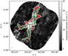 |
Fig. A.1 FilFinder filamentary identification. The background indicates the moment 0 map of the extracted N2H+ isolated components. The white contour shows the area where FilFinder identifies multiple filamentary structures (red and green lines). We remove the small-scale structures (in red) by “pruning” the skeleton structure from medskel, obtaining the main filaments of G353. We represent these filaments with green lines. |
Appendix B Examples of the isolated components fitting
In Sect. 3.1 we decomposed the multiple isolated component emission using PySpecKit. In Fig. B.1, we present the results of the Gaussian fitting for the high S/N spectra shown in Fig. 2 (panels c, e, and f).
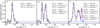 |
Fig. B.1 Gaussian velocity fits of the extracted N2H+ isolated components. In black we show the high S/N isolated components from panels c), e), and f) in Fig. 2. The individual Gaussian components and the obtained model are represented with dashed blue and solid red lines, respectively. On the right side of each panel we indicate the peak intensity (I), the velocity centroid (v), and velocity dispersion (σ) of each Gaussian component. The notations 1st, 2nd, and 3rd indicate the Gaussian velocity components from left to right. |
Appendix C DCN and N2H+ derived core velocity
In Table C.1 we provide the 1.3 mm core velocities obtained from DCN & N2H+ data (see Sect. 4.2), complementing the published DCN core velocities catalog from Cunningham et al. (2023). In the last column we indicate the number of N2H+ velocity components detected in these cores.
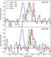 |
Fig. C.1 DCN and N2H+ normalized mean spectrum of cores 35 (top) and 46 (bottom). We show the multiple N2H+ isolated velocity components with blue, red, and green colors. We present the DCN emission in black. We see a match between the DCN emission and one of the N2H+ velocity components. We determine the N2H+ velocity for 11 cores with no DCN velocity fits. These are listed in Table C.1. |
1.3 mm core catalog of DCN & N2H+ velocities.
Appendix D V-shaped structures
In Sect. 5.3, we characterized the most prominent V-shaped structure we detect in Fig. 9. We repeated this process for the other eight different V-shaped structures, including the linear fits to the velocity gradients. In Fig. D.1, we indicate the V-shapes location in PV space with dark points, arrows, and their IDs. In Fig. D.2, we present individual close-ups for each V-shape. In Table D.1 we list their VGs, timescales, H2 masses, and mass accretion rates.
Here we list a few clarifications due to projection effects seen in these V-shaped structures:
In position-position space, only V-shape “B” presents a core within a ~beam size from its apex. This continuum core, core “7”, has a mass of ~6 M⊙.
For V-shape “A”, the 1.3 mm core with DCN single velocity component, located at the apex of this V-shape, is not spatially related with it.
In V-shapes “G” and “H” we see the same 1.3 mm cores with N2H+ velocities. These V-shapes are not the same distribution. They are overlapped in PV space and spatially separated by ~10″.
We improve the clarity of V-shape “B” by rotating the data in PP space by 80° counter-clockwise. We apply this process for V-shapes “E”, “G”, and “H” with an angle of 33° clockwise.
V-shapes G and H overlap in PV space but these are structures spatially separated.
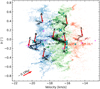 |
Fig. D.1 V-shapes location in PV space. We highlight the V-shapes listed in Table D.1 with black points and indicate them with red arrows and their ID. The core velocities and the N2H+ velocity distributions follow the same definitions from the top right panel in Fig. 9. V-shapes G and H overlap in PV space but these structures are spatially separated (left panel). |
Characterized V-shaped structures.
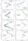 |
Fig. D.2 V-shaped structures listed in Table D.1, with the exception of “C” shown in Fig. 10. We indicate the “V-shape ID” from Table D.1 at the top/bottom left corner of each plot. The colors of the distributions, DCN and DCN & N2H+ derived core velocities, and beam size follow the same color and marker convention from Fig. 9. See Appendix D for clarifications regarding projection effects on these diagrams. |
Appendix E SiO Intensity-weighted position-velocity diagram
To create the SiO intensity-weighted PV diagram, first, we removed most of the noisy spectra by considering data with S/N ≥ 2.5. Then, we estimated the integrated intensity and velocity centroid at each pixel. We found improvements in our cleaning by using only spectra with integrated intensity ≥ 4 Kkm s–1. Using the coordinate, integrated-intensity, and velocity centroid of each spectrum, we create the SiO intensity-weighted PV diagrams we show in E.1.
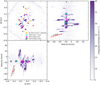 |
Fig. E.1 ALMA-IMF 12 m SiO equivalent of Fig. 9 using data from Cunningham et al. (2023). For the cores, we use the same marker and color convention from Fig. 9. With filled blue, red, and ‘red+blue’ circles we represent the SiO outflow candidates (Towner et al. 2024). With red arrows we indicate a VG = 400 km s–1 pc–1 corresponding to a timescale tVG = 2.5 kyr. The velocity range (∆V) covered by the SiO emission is ~80km s–1, about 10 times the velocity range traced by N2H+. This velocity difference suggests that SiO is tracing processes (outflows) ~100 times more energetic (ek = ∆V/2) than N2H+ (possibly infall). |
Appendix F G353 power law density profile
Here we provide the derivation of the density profile used for the gravitationally collapsing sphere. We assumed a power law density profile defined as:
 (F.1)
(F.1)
in which γ = 5.65 provides a good fit to the edges of the PV distribution seen in Fig. 8.
To determine the value of ρ0 , we integrated this expression in a sphere (Eq. (F.2)), with rmin < r < 0.5 pc. Based on different tests, probing total masses from 50 – 103 M⊙ and γ values from 2 – 6, we set the total mass of the sphere to 150 M⊙. We defined rmin ~ 0.007 pc which corresponds to the pixel size of the N2H+ data at a distance of 2 kpc.
 (F.2)
(F.2)
 (F.3)
(F.3)
 (F.4)
(F.4)
in which Menc(r = 0.5 pc) = 150 M⊙, rmin = 7 × 10⁻³ pc, and γ = 5.65, from Eq. (F.4), we obtained:
 (F.5)
(F.5)
References
- Álvarez-Gutiérrez, R. H., Stutz, A. M., Law, C. Y., et al. 2021, ApJ, 908, 86 [CrossRef] [Google Scholar]
- André, P., Men’shchikov, A., Bontemps, S., et al. 2010, A&A, 518, L102 [NASA ADS] [CrossRef] [EDP Sciences] [Google Scholar]
- Anglada, G., Rodriguez, L. F., Canto, J., Estalella, R., & Lopez, R. 1987, A&A, 186, 280 [NASA ADS] [Google Scholar]
- Armante, M., Gusdorf, A., Louvet, F., et al. 2024, A&A, 686, A122 [NASA ADS] [CrossRef] [EDP Sciences] [Google Scholar]
- Bastian, N., Covey, K. R., & Meyer, M. R. 2010, ARA&A, 48, 339 [Google Scholar]
- Bergin, E. A., Alves, J., Huard, T., & Lada, C. J. 2002, ApJ, 570, L101 [NASA ADS] [CrossRef] [Google Scholar]
- Bonfand, M., Csengeri, T., Bontemps, S., et al. 2024, A&A, 687, A163 [NASA ADS] [CrossRef] [EDP Sciences] [Google Scholar]
- Bonne, L., Bontemps, S., Schneider, N., et al. 2020, A&A, 644, A27 [EDP Sciences] [Google Scholar]
- Bonne, L., Bontemps, S., Schneider, N., et al. 2023, ApJ, 951, 39 [CrossRef] [Google Scholar]
- Busquet, G., Zhang, Q., Palau, A., et al. 2013, ApJ, 764, L26 [NASA ADS] [CrossRef] [Google Scholar]
- Caselli, P., Myers, P. C., & Thaddeus, P. 1995, ApJ, 455, L77 [Google Scholar]
- Caselli, P., Myers, P. C., & Thaddeus, P. 1995, ApJ, 455, L77 [Google Scholar]
- Caselli, P., Benson, P. J., Myers, P. C., & Tafalla, M. 2002a, ApJ, 572, 238 [Google Scholar]
- Caselli, P., Walmsley, C. M., Zucconi, A., et al. 2002b, ApJ, 565, 344 [Google Scholar]
- Cazzoli, G., Corbelli, G., Degli Esposti, C., & Favero, P. 1985, Chem. Phys. Lett., 118, 164 [Google Scholar]
- Chen, H.-R. V., Zhang, Q., Wright, M. C. H., et al. 2019, ApJ, 875, 24 [Google Scholar]
- Csengeri, T., Bontemps, S., Schneider, N., Motte, F., & Dib, S. 2011, A&A, 527, A135 [NASA ADS] [CrossRef] [EDP Sciences] [Google Scholar]
- Csengeri, T., Bontemps, S., Wyrowski, F., et al. 2017, A&A, 601, A60 [NASA ADS] [CrossRef] [EDP Sciences] [Google Scholar]
- Cunningham, N., Lumsden, S. L., Cyganowski, C. J., Maud, L. T., & Purcell, C. 2016, MNRAS, 458, 1742 [NASA ADS] [CrossRef] [Google Scholar]
- Cunningham, N., Ginsburg, A., Galván-Madrid, R., et al. 2023, A&A, 678, A194 [NASA ADS] [CrossRef] [EDP Sciences] [Google Scholar]
- Díaz-González, D. J., Galván-Madrid, R., Ginsburg, A., et al. 2023, ApJS, 269, 55 [CrossRef] [Google Scholar]
- Fernández-López, M., Arce, H. G., Looney, L., et al. 2014, ApJ, 790, L19 [Google Scholar]
- Galván-Madrid, R., Zhang, Q., Keto, E., et al. 2010, ApJ, 725, 17 [Google Scholar]
- Galván-Madrid, R., Liu, H. B., Zhang, Z. Y., et al. 2013, ApJ, 779, 121 [CrossRef] [Google Scholar]
- Ginsburg, A., & Mirocha, J. 2011, PySpecKit: Python Spectroscopic Toolkit, Ver. 0.1.23, Astrophysics Source Code Library [record ascl:1109.001] [Google Scholar]
- Ginsburg, A., Sokolov, V., de Val-Borro, M., et al. 2022, AJ, 163, 291 [NASA ADS] [CrossRef] [Google Scholar]
- Gómez, G. C., & Vázquez-Semadeni, E. 2014, ApJ, 791, 124 [Google Scholar]
- González Lobos, V., & Stutz, A. M. 2019, MNRAS, 489, 4771 [CrossRef] [Google Scholar]
- Hacar, A., Tafalla, M., Forbrich, J., et al. 2018, A&A, 610, A77 [NASA ADS] [CrossRef] [EDP Sciences] [Google Scholar]
- Henshaw, J. D., Caselli, P., Fontani, F., Jiménez-Serra, I., & Tan, J. C. 2014, MNRAS, 440, 2860 [Google Scholar]
- Henshaw, J. D., Ginsburg, A., Haworth, T. J., et al. 2019, MNRAS, 485, 2457 [Google Scholar]
- Henshaw, J. D., Kruijssen, J. M. D., Longmore, S. N., et al. 2020, Nat. Astron., 4, 1064 [CrossRef] [Google Scholar]
- Inoue, T., & Fukui, Y. 2013, ApJ, 774, L31 [Google Scholar]
- Inoue, T., Hennebelle, P., Fukui, Y., et al. 2018, PASJ, 70, S53 [NASA ADS] [Google Scholar]
- Koch, E. W., & Rosolowsky, E. W. 2015, MNRAS, 452, 3435 [Google Scholar]
- Kumar, M. S. N., Arzoumanian, D., Men’shchikov, A., et al. 2022, A&A, 658, A114 [NASA ADS] [CrossRef] [EDP Sciences] [Google Scholar]
- Kuznetsova, A., Hartmann, L., & Ballesteros-Paredes, J. 2015, ApJ, 815, 27 [NASA ADS] [CrossRef] [Google Scholar]
- Kuznetsova, A., Hartmann, L., & Ballesteros-Paredes, J. 2018, MNRAS, 473, 2372 [NASA ADS] [CrossRef] [Google Scholar]
- Lee, C. W., Myers, P. C., & Tafalla, M. 1999, ApJ, 526, 788 [NASA ADS] [CrossRef] [Google Scholar]
- Lee, C. W., Myers, P. C., & Tafalla, M. 2001, ApJS, 136, 703 [NASA ADS] [CrossRef] [Google Scholar]
- Lippok, N., Launhardt, R., Semenov, D., et al. 2013, A&A, 560, A41 [NASA ADS] [CrossRef] [EDP Sciences] [Google Scholar]
- Liu, H. B., Galván-Madrid, R., Jiménez-Serra, I., et al. 2015, ApJ, 804, 37 [Google Scholar]
- Liu, H.-L., Stutz, A., & Yuan, J.-H. 2019, MNRAS, 487, 1259 [Google Scholar]
- Liu, T., Evans, N. J., Kim, K.-T., et al. 2020, MNRAS, 496, 2790 [Google Scholar]
- Louvet, F., Sanhueza, P., Stutz, A., et al. 2024, A&A, in press, https://doi.org/10.1051/0004-6361/202345986 [Google Scholar]
- Mardones, D., Myers, P. C., Tafalla, M., et al. 1997, ApJ, 489, 719 [Google Scholar]
- Men’shchikov, A. 2021, A&A, 649, A89 [EDP Sciences] [Google Scholar]
- Minh, Y. C., Liu, H. B., Galvan-Madrid, R., et al. 2018, ApJ, 864, 102 [NASA ADS] [CrossRef] [Google Scholar]
- Motte, F., Bontemps, S., & Louvet, F. 2018, ARA&A, 56, 41 [NASA ADS] [CrossRef] [Google Scholar]
- Motte, F., Bontemps, S., Csengeri, T., et al. 2022, A&A, 662, A8 [NASA ADS] [CrossRef] [EDP Sciences] [Google Scholar]
- Myers, P. C. 2009, ApJ, 700, 1609 [Google Scholar]
- Nony, T., Galván-Madrid, R., Motte, F., et al. 2023, A&A, 674, A75 [NASA ADS] [CrossRef] [EDP Sciences] [Google Scholar]
- Offner, S. S. R., Clark, P. C., Hennebelle, P., et al. 2014, in Protostars and Planets VI, eds. H. Beuther, R. S. Klessen, C. P. Dullemond, & T. Henning, 53 [Google Scholar]
- Olguin, F. A., Sanhueza, P., Chen, H.-R. V., et al. 2023, ApJ, 959, L31 [NASA ADS] [CrossRef] [Google Scholar]
- Pan, S., Liu, H.-L., & Qin, S.-L. 2024, ApJ, 960, 76 [NASA ADS] [CrossRef] [Google Scholar]
- Peretto, N., Fuller, G. A., André, P., et al. 2014, A&A, 561, A83 [NASA ADS] [CrossRef] [EDP Sciences] [Google Scholar]
- Peretto, N., Rigby, A. J., Louvet, F., et al. 2023, MNRAS, 525, 2935 [NASA ADS] [CrossRef] [Google Scholar]
- Pouteau, Y., Motte, F., Nony, T., et al. 2023, A&A, 674, A76 [NASA ADS] [CrossRef] [EDP Sciences] [Google Scholar]
- Rawat, V., Samal, M. R., Walker, D. L., et al. 2024, MNRAS, 528, 2199 [NASA ADS] [CrossRef] [Google Scholar]
- Redaelli, E., Bovino, S., Sanhueza, P., et al. 2022, ApJ, 936, 169 [NASA ADS] [CrossRef] [Google Scholar]
- Reyes-Reyes, S. D., Stutz, A. M., Megeath, S. T., et al. 2024, MNRAS, 529, 2220 [NASA ADS] [CrossRef] [Google Scholar]
- Sanhueza, P., Contreras, Y., Wu, B., et al. 2019, ApJ, 886, 102 [Google Scholar]
- Sanhueza, P., Girart, J. M., Padovani, M., et al. 2021, ApJ, 915, L10 [NASA ADS] [CrossRef] [Google Scholar]
- Schuller, F., Menten, K. M., Contreras, Y., et al. 2009, A&A, 504, 415 [NASA ADS] [CrossRef] [EDP Sciences] [Google Scholar]
- Smith, R. J., Shetty, R., Stutz, A. M., & Klessen, R. S. 2012, ApJ, 750, 64 [NASA ADS] [CrossRef] [Google Scholar]
- Storm, S., Mundy, L. G., Fernández-López, M., et al. 2014, ApJ, 794, 165 [NASA ADS] [CrossRef] [Google Scholar]
- Stutz, A. M. 2018, MNRAS, 473, 4890 [NASA ADS] [CrossRef] [Google Scholar]
- Stutz, A. M., & Gould, A. 2016, A&A, 590, A2 [NASA ADS] [CrossRef] [EDP Sciences] [Google Scholar]
- Stutz, A. M., & Kainulainen, J. 2015, A&A, 577, L6 [NASA ADS] [CrossRef] [EDP Sciences] [Google Scholar]
- Stutz, A. M., Gonzalez-Lobos, V. I., & Gould, A. 2018, arXiv e-prints [arXiv:1807.11496] [Google Scholar]
- Tafalla, M., Myers, P. C., Caselli, P., & Walmsley, C. M. 2004, A&A, 416, 191 [NASA ADS] [CrossRef] [EDP Sciences] [Google Scholar]
- Tafalla, M., Usero, A., & Hacar, A. 2021, A&A, 646, A97 [NASA ADS] [CrossRef] [EDP Sciences] [Google Scholar]
- Tobin, J. J., Hartmann, L., Bergin, E., et al. 2012, ApJ, 748, 16 [Google Scholar]
- Towner, A. P. M., Ginsburg, A., Dell’Ova, P., et al. 2024, ApJ, 960, 48 [NASA ADS] [CrossRef] [Google Scholar]
- Ungerechts, H., Bergin, E. A., Goldsmith, P. F., et al. 1997, ApJ, 482, 245 [Google Scholar]
- Wienen, M., Wyrowski, F., Menten, K. M., et al. 2015, A&A, 579, A91 [NASA ADS] [CrossRef] [EDP Sciences] [Google Scholar]
- Zhou, J.-W., Liu, T., Evans, N. J., et al. 2022, MNRAS, 514, 6038 [NASA ADS] [CrossRef] [Google Scholar]
- Zhou, J. W., Wyrowski, F., Neupane, S., et al. 2023, A&A, 676, A69 [NASA ADS] [CrossRef] [EDP Sciences] [Google Scholar]
Proposal ID 2017.1.01355.L, PIs: Motte, Ginsburg, Louvet, Sanhueza.
Available at www.almaimf.com
All Tables
All Figures
|
Fig. 1 Composite image of G353: IRAC 3.6 µm (in blue), 4.5 µm (green), and 5.8 µm (red). We indicate the ALMA-IMF N2H+ (1–0) coverage with a light green contour. We highlight ATLASGAL emission (870 µm) at 40 mJy beam−1 with the gray contour, corresponding roughly to a Herschel-derived N(H) of ~ 5.5 1022 cm−2. |
| In the text | |
|
Fig. 2 N2H+ spectra involved in our isolated component extraction procedure. Panel a: normalized average N2H+ spectrum (solid black line) over the entire region. We show the location of the mean peak of the isolated component (dashed black line) and the “mean dip” (dashed gray line), see text. Middle and right panels: normalized example spectra (within a pixel) of the N2H+ isolated velocity component extraction procedure (see Sect. 3). We show G353 N2H+ spectra with solid black lines and the extracted isolated component, along with emission-free channels, with dashed red lines. Panel d: expected N2H+ emission for an excitation temperature of 15 K, an opacity of 1, velocity centroid of −17 km s−1, and a line width of 0.2 km s−1. We see the seven hyperfine components characteristic of this tracer, in which the most blueshifted corresponds to the isolated component. To derive this emission we use “n2hp_vtau” model from PySpecKit. In panels b, c, e, and f) we indicate Vmean dip with a dashed gray line. We present data with S /N < 5 in panel b, in which we make a rough extraction based on the Vmean dip. We show data with S /N ≥ 5 in panels c, e, and f, presenting clear single, double, and triple N2H+ isolated velocity components, respectively. In these examples we represent the selected velocity guess that separates the isolated component emission from the main line emission with dashed blue lines. The offset positions (Δl, Δb) of the spectra in panels b, c, e, and f are (0.68 pc, 0.27 pc), (0.12pc, −0.28 pc), (−0.08 pc, 0.47 pc), and (0.16pc, −0.07pc), respectively. These offsets are estimated relative to the center of the region (see Sect. 1). |
| In the text | |
|
Fig. 3 G353 N2H+ isolated component S/N map. The white contour indicates the location of data with an isolated component S/N ≥ 5. We show the location of the 1.3 mm cores presented in Louvet et al. (2024) with black ellipses and are located in regions with S/N ≥ 15. We indicate the beam size of these data with a gray ellipse at the bottom left corner. Outside the S/N contour we make a rough extraction of the isolated component (see text). For data inside the S/N contours, we implement a procedure based on detection of peaks and valleys, to individually extract high (≥5) S/N isolated components (see Sect. 3). |
| In the text | |
|
Fig. 4 Moment 0 map of the extracted N2H+ isolated component emission. We use the FilFinder Python package to identify the main filamentary structure present in G353 (see Appendix A). We identify three filaments (F1, F2, and F3; green lines) converging toward the central hub. The location of most of the 1.3 mm cores (red ellipses), projected in the POS, lie on top of the spine of these filaments, specially in the hub. |
| In the text | |
|
Fig. 5 Spatial distribution of the modeled N2H+ isolated velocity components. We indicate the main filament structure with green lines (see Fig. 4). In blue, green, and red we indicate the first, second, and third velocity components, respectively. We indicate the beam size of these data with a gray ellipse at the bottom left corner. The emission of the first and second components is more extended and intense than the third, most red-shifted velocity component. The 1.3 mm cores match regions with high integrated intensity, mostly traced by the first and second velocity components. |
| In the text | |
|
Fig. 6 Spatial distribution of the modeled N2H+ isolated component spectra. These models are composed by up to three Gaussian velocity components. The 1.3 mm cores and beam size are the same as in Fig. 3. Most of the 1.3 mm cores are located in regions with spectra presenting two to three velocity components (see Sect. 4.1). |
| In the text | |
|
Fig. 7 Normalized velocity centroid distributions of each N2H+ Gaussian velocity component. The velocities at the peak of the distributions are −26.9 km s−1, −24.7 km s−1, and −23.3 km s−1 for component 1 (blue), 2 (green), and 3 (red), respectively (see Sect. 4.1). |
| In the text | |
|
Fig. 8 “Traditional” PV diagram of the N2H+ modeled isolated components, created by collapsing the l coordinate. Δb indicates the distance along b in pc, relative to the center of G353, assuming a distance of 2 kpc (Motte et al. 2022). The colormap indicates the total intensity along l. With fuchsia and black crosses we show the 1.3 mm cores with single and complex DCN velocities detections, respectively (Cunningham et al. 2023). With dark cyan “×” markers we show the 1.3 mm cores with velocities derived from DCN and N2H+ data (see Sect. 4.2). The size of the markers indicate relative mass (Louvet et al. 2024). Black contours indicate total intensities at 40, 160, 280, and 400 K. We see a large-scale velocity spread (ΔV ~ 8 km s−1) around Δb ~ −0.3 pc − 0.13 pc (see also Sect. 5.2). We show the major axis of the beam and the channel width with a white rectangle at the bottom left corner. |
| In the text | |
|
Fig. 9 N2H+ intensity-weighted position-position and PV diagrams of G353. Top left: spatial distribution of the fitted N2H+ Gaussian isolated velocity components (blue, green, and red, see Sect. 4.1). Ellipses indicate the location of the 1.3 mm continuum cores (Louvet et al. 2024). Orange indicates cores with no DCN detections. Fuchsia and black represent cores with single and complex DCN velocities (Cunningham et al. 2023). DCN & N2H+ cores are indicated with cyan. We show the beam size with a gray ellipse in the bottom left corner. Top right and bottom left: intensity-weighted PV diagrams along the b and l coordinates, respectively. For the 1.3 mm core velocities we use the same colors and markers convention from Fig. 8. For reference we indicate with a red arrow, in both the top right and bottom left panels, a VG of 10 km s−1 pc−1 corresponding to a timescale of ~0.1 Myr. We see multiple V-shapes near the location of cores across all velocities in the PV diagrams, more prominently in the top right panel (see Fig. D.1). The most prominent V-shape is located in the blue component, at (V, ∆b) ~ (−20.5km s−1, −0.14 pc) (see Sect. 5.2). We provide an interactive 3D PPV diagram online. |
| In the text | |
|
Fig. 10 Zoomed-in version of the top right panel of Fig. 9, centered at the prominent blue V-shape (“C”) located at (∆b, V) = (−0.14pc, −20.5 km s−1). We indicate the major axis of the cores with vertical lines in fuchsia (DCN single) and cyan (N2H+), similarly we represent the major axis of the beam with a vertical orange line. We apply linear fits to the upper and lower distributions, represented by darker points. These points are selected based on an integrated intensity threshold (see Sect. 5.3). We weight each point by their integrated intensity and derive VGs from the slope of these linear fits. The range of the obtained VGs is ~13 – 18 km s−1 pc−1. We defined the timescale associated with the VG as tVG = VG−1, being in the range of ~50–70 kyr. We show eight more well characterized V-shapes in Appendix D. |
| In the text | |
|
Fig. 11 Left panel: integrated intensity map of the modeled N2H+ isolated component within a region of radius of 0.1 pc, centered at V-shape “C”. With boxes in shades of green and yellow, we indicate the different paths taken to create the PV diagrams shown on the right panel. The area covered by these four PVs matches the extent of this V-shape (see Fig. 12). The 1.3 mm cores are indicated using the same convention from Fig. 9. For the cores within the radius of 0.1 pc we indicate their IDs in black. Right panel: PV diagrams associated with the colored rectangles in the left panel. At the bottom right corner of each sub panel, with colored values, we indicate the angle (counter-clockwise) of each PV path. The PV paths match the V-shape coverage (right panel of Fig. 12). We see the overall structure of this V-shape persists at different angles, indicating that these structures are not a result of projection in the POS. |
| In the text | |
|
Fig. 12 Multi-tracer diagram at the location of the main blue V-shape of G353 (Sect. 5.3). The different panels show the step by step construction of the final plot (right panel). Left panel: the black to white background shows the 1.3 mm continuum emission from Díaz-González et al. (2023). With black ellipses we show the 1.3 mm continuum cores from Louvet et al. (2024). With black text we indicate the IDs of the cores closest to the center of the V-shape, marked with a fuchsia “×”. We indicate the barycenter of cores 2 & 3 (see Fig. 11) with a yellow “×”. Filled contours represent the CO (2–1) emission in the velocity ranges of −50 km s−1 to −15 km s−1 (cyan) and 15 km s−1 to 50 km s−1 (beige), relative to the Vlsr = −17 km s−1 of G353. With a white contour we indicate the log (N(H2) cm2) = 23.3. Middle panel: in addition to the left panel, we include the SiO (5–4) emission with blue and red contours in the same (negative and positive) velocity range as with CO. The pink contour indicates the integrated intensity of the most blueshifted modeled N2H+ Gaussian velocity component (see Fig. 9; blue distribution), at a value of 7 K km s−1. Right panel: with open circles we show the location of the data composing the main N2H+ blue V-shape. The colors indicate their velocity centroid, and their (increasing) size indicates how close the gas velocities are to the velocity apex of the V-shape. This VG seems to converge to the barycenter of cores 2 and 3, and it is oriented along filament “F3”. |
| In the text | |
|
Fig. 13 V-shapes location on the plane of the sky. We indicate the position of each V-shape with colored points and their ID with black text. With red lines we show the filamentary structure identified in Sect. 3.2. In the background we show the integrated intensity map of all three velocity components, similarly as in Fig. 9. We see most of the V-shapes are located at the hub. |
| In the text | |
|
Fig. 14 Mean spectra within a 1.14″ (~0.01 pc) radius around the location of the main blue V-shape (pink “×” in Fig. 12). Both N2H+ and H2CO show blue asymmetry, known to characterize infall motions. The difference in velocity between the two N2H+ peaks is ~2.5 km s−1. |
| In the text | |
|
Fig. 15 PV coverage of a gravitationally collapsing sphere. The white contour represents the coverage of the synthetic radial velocities derived from this model (Sect. 6). The background and cores are the same as in Fig. 8. For the modeled sphere we set its total mass to 150 M⊙, within a radius of 0.5 pc. |
| In the text | |
|
Fig. A.1 FilFinder filamentary identification. The background indicates the moment 0 map of the extracted N2H+ isolated components. The white contour shows the area where FilFinder identifies multiple filamentary structures (red and green lines). We remove the small-scale structures (in red) by “pruning” the skeleton structure from medskel, obtaining the main filaments of G353. We represent these filaments with green lines. |
| In the text | |
|
Fig. B.1 Gaussian velocity fits of the extracted N2H+ isolated components. In black we show the high S/N isolated components from panels c), e), and f) in Fig. 2. The individual Gaussian components and the obtained model are represented with dashed blue and solid red lines, respectively. On the right side of each panel we indicate the peak intensity (I), the velocity centroid (v), and velocity dispersion (σ) of each Gaussian component. The notations 1st, 2nd, and 3rd indicate the Gaussian velocity components from left to right. |
| In the text | |
|
Fig. C.1 DCN and N2H+ normalized mean spectrum of cores 35 (top) and 46 (bottom). We show the multiple N2H+ isolated velocity components with blue, red, and green colors. We present the DCN emission in black. We see a match between the DCN emission and one of the N2H+ velocity components. We determine the N2H+ velocity for 11 cores with no DCN velocity fits. These are listed in Table C.1. |
| In the text | |
|
Fig. D.1 V-shapes location in PV space. We highlight the V-shapes listed in Table D.1 with black points and indicate them with red arrows and their ID. The core velocities and the N2H+ velocity distributions follow the same definitions from the top right panel in Fig. 9. V-shapes G and H overlap in PV space but these structures are spatially separated (left panel). |
| In the text | |
|
Fig. D.2 V-shaped structures listed in Table D.1, with the exception of “C” shown in Fig. 10. We indicate the “V-shape ID” from Table D.1 at the top/bottom left corner of each plot. The colors of the distributions, DCN and DCN & N2H+ derived core velocities, and beam size follow the same color and marker convention from Fig. 9. See Appendix D for clarifications regarding projection effects on these diagrams. |
| In the text | |
|
Fig. E.1 ALMA-IMF 12 m SiO equivalent of Fig. 9 using data from Cunningham et al. (2023). For the cores, we use the same marker and color convention from Fig. 9. With filled blue, red, and ‘red+blue’ circles we represent the SiO outflow candidates (Towner et al. 2024). With red arrows we indicate a VG = 400 km s–1 pc–1 corresponding to a timescale tVG = 2.5 kyr. The velocity range (∆V) covered by the SiO emission is ~80km s–1, about 10 times the velocity range traced by N2H+. This velocity difference suggests that SiO is tracing processes (outflows) ~100 times more energetic (ek = ∆V/2) than N2H+ (possibly infall). |
| In the text | |
Current usage metrics show cumulative count of Article Views (full-text article views including HTML views, PDF and ePub downloads, according to the available data) and Abstracts Views on Vision4Press platform.
Data correspond to usage on the plateform after 2015. The current usage metrics is available 48-96 hours after online publication and is updated daily on week days.
Initial download of the metrics may take a while.