| Issue |
A&A
Volume 617, September 2018
|
|
|---|---|---|
| Article Number | A67 | |
| Number of page(s) | 43 | |
| Section | Interstellar and circumstellar matter | |
| DOI | https://doi.org/10.1051/0004-6361/201833015 | |
| Published online | 13 September 2018 | |
Bipolar H II regions
II. Morphologies and star formation in their vicinities
1
Aix-Marseille Université, CNRS, LAM, Laboratoire d’Astrophysique de Marseille,
Marseille,
France
e-mail: This email address is being protected from spambots. You need JavaScript enabled to view it.
2
Graduate Institute of Astronomy, National Central University 300,
Jhongli City,
Taoyuan County
32001,
Taiwan
3
Department of Physics & Astronomy, West Virginia University,
Morgantown,
WV 26506,
USA
4
Center for Gravitational Waves and Cosmology, West Virginia University, Chestnut Ridge Research Building,
Morgantown,
WV 26505,
USA
5
Adjunct Astronomer at the Green Bank Observatory,
PO Box 2,
Green Bank,
WV 24944,
USA
6
INAF-Istituto Fisica Spazio Interplanetario,
Via Fosso del Cavaliere 100,
00133
Roma,
Italy
Received:
13
March
2018
Accepted:
5
May
2018
Abstract
Aims. We aim to identify bipolar Galactic H II regions and to understand their parental cloud structures, morphologies, evolution, and impact on the formation of new generations of stars.
Methods. We use the Spitzer-GLIMPSE, Spitzer-MIPSGAL, and Herschel-Hi-GAL surveys to identify bipolar H II regions and to examine their morphologies. We search for their exciting star(s) using NIR data from the 2MASS, UKIDSS, and VISTA surveys. Massive molecular clumps are detected near these bipolar nebulae, and we estimate their temperatures, column densities, masses, and densities. We locate Class 0/I young stellar objects (YSOs) in their vicinities using the Spitzer and Herschel-PACS emission.
Results. Numerical simulations suggest bipolar H II regions form and evolve in a two-dimensional flat- or sheet-like molecular cloud. We identified 16 bipolar nebulae in a zone of the Galactic plane between ℓ ± 60° and |b| < 1°. This small number, when compared with the 1377 bubble H II regions in the same area, suggests that most H II regions form and evolve in a three-dimensional medium. We present the catalogue of the 16 bipolar nebulae and a detailed investigation for six of these. Our results suggest that these regions formed in dense and flat structures that contain filaments. We find that bipolar H II regions have massive clumps in their surroundings. The most compact and massive clumps are always located at the waist of the bipolar nebula, adjacent to the ionised gas. These massive clumps are dense, with a mean density in the range of 105 cm−3 to several 106 cm−3 in their centres. Luminous Class 0/I sources of several thousand solar luminosities, many of which have associated maser emission, are embedded inside these clumps. We suggest that most, if not all, massive 0/I YSO formation has probably been triggered by the expansion of the central bipolar nebula, but the processes involved are still unknown. Modelling of such nebula is needed to understand the star formation processes at play.
Key words: H II regions / dust, extinction / stars: formation
© ESO 2018
 Open Access article, published by EDP Sciences, under the terms of the Creative Commons Attribution License (http://creativecommons.org/licenses/by/4.0), which permits unrestricted use, distribution, and reproduction in any medium, provided the original work is properly cited.
1 Introduction
Long before the Herschel era, molecular clouds were known to exhibit rather complex geometries, including smaller substructures such as sheets and filaments (Schneider & Elmegreen 1979; de Geus et al. 1990; Mizuno et al. 1995; Goldsmith et al. 2008; Myers 2009). The unprecedented coverage and sensitivity of the Herschel observations have shown that filaments and filamentary structures (e.g. André et al. 2010; Molinari et al. 2010b; Wang et al. 2015) are closely tied to the star formation process as young protostars, and that bound prestellar cores are preferentially located within the dense filaments (Könyves et al. 2015; Marsh et al. 2016).
A growing body of evidence indicates that interstellar sheets and filaments play a vital role in the star formation process (e.g. André et al. 2014; Anathpindika & Freundlich 2015), including the formation of massive stars (e.g. Hill et al. 2011; Motte et al. 2018). Once a massive star forms, it photoionises its surroundings, forming an H II region. While still embedded in their natal molecular clouds, H II regions remain small and are classified as ultra-compact (UC: linear size < 0.1 pc) or compact (0.1–1 pc). Classical H II regions (size > 1 pc) correspond to a more evolved stage. Our understanding of the evolution and physics of H II regions comes mostly from studies that assume spherical symmetry. Classical H II regions can also show cometary and bipolar morphologies, although the latter is observed only in a few cases (e.g. Bally et al. 1983; Minier et al. 2013). The formation and evolution of spherical (e.g. Strömgren 1939; Kahn & Dyson 1965; Yorke 1986; Dyson & Williams 1997; Raga et al. 2012; Tremblin et al. 2014) and cometary or blister H II regions (e.g. Tenorio-Tagle 1979; Franco et al. 1990; Henney et al. 2005; Arthur & Hoare 2006; Steggles et al. 2017) have been relatively well-studied analytically and numerically.
To date, little numerical work has been devoted to the modelling and simulation of bipolar H II regions, primarily because no adequate attention has been paid to the identification and characterisation of such nebulae. In fact the only numerical work that reproduces the observed morphology of bipolar H II regions is done by Bodenheimer et al. (1979), who present a two-dimensional (2D) hydrodynamic simulation following the evolution of an H II region excited by a star lying in the symmetry plane of a flat homogeneous molecular cloud surrounded by a low-density medium. Recently, Wareing et al. (2017) using three-dimensional (3D) magnetohydrodynamic simulations found that when a massive star evolves in a sheet-like molecular cloud formed through the action of the thermal instability, the bubble that forms has a bipolar structure and a ring of swept-up material (see also, Wareing et al. 2018). Therefore, investigation of bipolar H II regions will add more insight into the nature of the molecular clouds in which they reside and the nature of clouds in general (see discussion in Anderson et al. 2011).
H II regions can trigger a new generation of star formation in their surroundings, either by sweeping ambient clouds into dense shells or by compressing nearby dense clouds into bound clumps/cores. In both cases, dense material eventually fragments to form new stars (for details, see the discussion in Deharveng et al. 2010), a process known as “triggering”. Prior work on triggering has focused exclusively on the winds and radiation from high-mass stars, and their impact on the surrounding cloud of uniform or power-law radial density profile (e.g. Whitworth et al. 1994; Hosokawa & Inutsuka 2005; Dale et al. 2007). For example, Dale et al. (2007), simulate the evolution of a spherical, uniform molecular cloud with an ionising source at its centre and find that the shell driven by the H II region fragments to form numerous self-gravitating objects that would form stars. Observational evidence of this process has been found at the edges of several H II regions in our Galaxy (e.g. Zavagno et al. 2010; Deharveng et al. 2012; Samal et al. 2014; Bernard et al. 2016; Liu et al. 2016), although disentangling true triggered stars from the spontaneously formed ones is still a subject of concern as the structure of the molecular clouds into which the H II region expands is often fractal and turbulent (see discussion in Walch et al. 2015; Dale et al. 2015). If it was true that bipolar H II regions form in a flat- or sheet-like filamentary molecular cloud, then one would expect the evolution and subsequent impact of the expanding H II region to be different from the spherical one. Numerical simulations by Fukuda & Hanawa (2000) suggest that H II region expansion near a filamentary molecular cloud can generate sequential waves of star-forming cores along the long axis of the filament on either side of the H II region.
In our previous work (Deharveng et al. 2015, hereafter Paper I) we presented multi-wavelength observations towards two bipolar H II regions. Based on the morphological comparison of the ionised gas of the H II region (which is often extended more than a few parsecs due to the effects of stellar feedback) and dense cold gas of the parental cloud, along with the velocity difference between ionised and molecular gas, we suggested that bipolar H II regions form in dense, flat, or sheet-like structures that contain filaments. In Paper I, we showed that due to the presence of dense filaments, bipolar H II regions can easily be mistaken for dual-bubble H II regions whose lobes are in contact when observed with Spitzer IRAC bands (e.g. see Sect. 3.1 of Paper I), or for cometary H II regions when observed at optical bands. Because of the high sensitivity and sub-parsec resolution, large-scale far-infrared (FIR) images from the Hi-Gal survey (Molinari et al. 2010a) allow us to study the cold dust properties of such regions over large scales. Analyses of column-density maps derived from Herschel observations have clearly shown the presence of cold dense filaments of high column density in bipolar H II regions that bisect their ionised lobes. Our results show that the parental cloud structure is important for the bipolar morphology of the H II region. We note that, while many spherical or irregularly shaped classical H II regions or bubbles have been identified in our Galaxy (e.g., Churchwell et al. 2006, 2007; Deharveng et al. 2010; Simpson et al. 2012), the observations of classical bipolar H II regions are still scarce; although our work has laid the foundations for the identification and investigation of a few more classical bipolar H II regions very recently (e.g. Xu et al. 2017; Panwar et al. 2017; Eswaraiah et al. 2017).
In this paper, we extend our study to six more bipolar H II regions in a continuation of our efforts to understand their cloud structure, morphology, evolution, and effect on the star formation processes in the parental cloud. The paper is organised as follows: Sect. 2 gives a summary of the observations used to identify candidate bipolar H II regions. These observations and the data reduction procedures are fully discussed in Paper I. Using the Spitzer Galactic Legacy Infrared Mid-Plane Survey Extraordinaire (GLIMPSE) and MIPS Inner Galactic Plane Survey (MIPSGAL) surveys, and the Herschel infrared Galactic Plane Survey (Hi-GAL), we have identified 16 candidate bipolar H II regions in a zone of the Galactic plane in the zone ℓ±60° and |b| < 1°. The catalogue of all the 16 candidate bipolar H II regions is given in Sect. 3. Six of these regions are studied in detail in this work and are presented in the Appendices. The other regions are the subject of a future paper. Section 3 also presents the overall morphology and physical conditions of the various components of interstellar medium (ISM) associated to bipolar H II regions, and discusses the general nature and properties of the stars, protostars, and dust clumps found in these regions. Section 4 discusses star formation in the vicinity of bipolar H II regions, especially in the context of triggered star formation. We give our conclusions in Sect. 5.
2 Methodology
As explainedin Paper I, in bipolar H II regions, the 8.0 μm emission is mostly due to the emission from polycyclic aromatic hydrocarbons (PAHs), which fluoresce in the immediate vicinity of the ionisation fronts (IFs). At 8.0 μm, these regions present two lobes separated bya narrow waist. At 24 μm, they are bright in the central region; this emission is due to very small grains located inside the ionised region and out of thermal equilibrium (Pavlyuchenkov et al. 2013). We use Spitzer images for identifying bipolar H II regions. Figure 1 shows an example of a bipolar H II region as seen by Spitzer (see also Fig. 4 of Paper I). We then use Herschel images to identify possible cold filaments by making Herschel column density and temperature maps. We subsequently check each bipolar H II region for the presence of radio continuum emission (using the NRAO VLA Sky Survey (NVSS), Sydney University Molonglo Sky Survey (SUMSS), and VLA Galactic Plane Survey (VGPS) surveys) to confirm the existence of a central H II region. Further, to study the star-formation around the bipolar H II regions, we explore their stellar, protostellar, and dense clump components using data from the Two Micron All Sky Survey (2MASS), UKIRT Infrared Deep Sky Survey (UKIDSS), and Visible and Infrared Survey Telescope for Astronomy (VISTA), Spitzer, and Herschel surveys (details about these datasets are given in Paper I).
In the following, we briefly outline our methodology for identifying and studying various components of the bipolar H II regions.Further details can be found in Paper I.
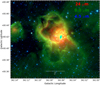 |
Fig. 1 Morphology of a bipolar H II region in the Spitzer bands. Red is the MIPSGAL image at 24 μm, green is the GLIMPSE image at 8.0 μm, and blue is the GLIMPSE image at 4.5 μm. |
2.1 Creation of dust temperature and column density maps
We create dust temperature and column density maps using the same procedure detailed in Sect. 4.1 of Paper I. Briefly, we use the Herschel Hi-GAL images at 160, 250, 350, and 500 μm, which are smoothed and regridded to the resolution (~37′′) and pixel size (11.5′′) of the 500 μm map. The spectral energy distribution (SED) of each pixel is then fitted by a single-temperature modified black-body model. No background emission is subtracted from the images prior to the SED fitting. Thus, the temperature maps represent the mean temperature for all material along the line of sight, weighted by the intensity of the emission. The dust opacities adopted for the SED fitting are κν = 35.2, 14.4, 7.3, and 3.6 cm2 g−1 at 160, 250, 350, and 500 μm, respectively (see Table 1 of Deharveng et al. 2012, and discussions therein). Uncertainties on derived dust temperatures are on the order of 2 K, mainly due to the uncertainty in the dust opacities (see discussion in Paper I).
We use the temperature maps to obtain high-resolution column density maps. We regrid the temperature maps to the resolution of the 250 μm data (18′′), then estimate the column density using the intensity of the 250 μm map, the temperature from the regridded temperature map, and Eq. (2) of Paper I. We assume that the regridded temperaturedoes not differ strongly from the one that would be obtained if all the maps had the resolution of the 250 μm observations.
We stress that the column density of a structure can depend upon its size. For example, if the size of a structure (a clump, a core, a filament) is smaller than 18′′, then this structure is smoothed out in our maps and its peak column density is underestimated; this effect can be important for distant regions1 (see also discussions in Baldeschi et al. 2017).
2.2 Characterisation of dust clumps
As in Paper I, for each region we only discuss the highest column density structures. We estimate the mass of the central region of such structures by integrating the column density in an aperture following the level at the column density peak’s half intensity. Although this approach is more suitable for compact clumps, it is interesting for two reasons: 1) if the clump can be approximated by an elliptical Gaussian of uniform temperature, its total mass is twice the mass measured using an aperture following the level at half the peak’s value; and 2) the derived mass is not dependent on the beam size, which therefore allows us to compare the masses (and mean density) of clumps at different distances and angular sizes. We estimate the mean volume density in the central regions of the clumps, using their mass and beam deconvolved size obtained for the aperture following the level at half the maximum value, assuming a spherical morphology and a homogeneous medium.
While estimating the parameters of the dense structures, we have subtracted a background column density value, which we estimate from regions close to the structures. This is done to minimise the effects of emission along the line of sight.
2.3 Search for ionised region and associated exciting star or cluster
We use Hα maps (from the SuperCOSMOS survey) and radio-continuum maps (from the NVSS, VGPS, and SUMSS surveys) to search for emission from the ionised gas in the central region of the bipolar H II regions. We then search for the exciting stars within the central ionised region of each bipolar nebula. The best way to identify O- and early B-type stars is through spectrophotometry, but these data do not exist for most of the bipolar nebulae in our sample. We therefore use two other methods:
- (i)
When the distance to the bipolar nebula is known but the exciting star is not (possibly due to high extinction), we use the radio continuum flux of the H II region to estimate the likely spectral type of the probable ionising star. Using Eq. (1) in Simpson & Rubin (1990), and assuming an electron temperature of 8000 K for the H II region and a ratio He+/H+ = 0.05, we estimate the ionising photon flux, and spectral type adopting the calibration of Martins et al. (2005) for O stars and of Smith et al. (2002) for early B stars. Here we assume that the exciting star is single and that no ionising photons are absorbed in the ionised region or leaked out into the interstellar medium (ISM).
- (ii)
When the distance to the H II region is known and the exciting cluster is visible, we use the near-infrared (NIR) catalogues to identify the exciting star (see Fig. 3 of Paper I). The exciting cluster can be undetectable in the NIR if it is hidden behind dense filamentary cloud located along the line of sight, at the waist of the nebula. The spectral types of massive stars derived using NIR data can be uncertain, particularly if the stars have excess emission in the NIR bands. To minimise the effect of excess emission, we mostly use J-band luminosity of the potential sources. We use the absolute magnitudes and colours of Martins & Plez (2006) to characterise O-type stars. For less massive stars, we use the data table of Pecaut & Mamajek (2013). When possible, we use both the above criteria to determine the distance to the bipolar H II regions (e.g. see discussion in the Sect. 6.1 of Paper I).
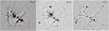 |
Fig. 2 Unsharp-masked images of G049.99–00.13 at 70, 24, and 8 μm. |
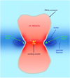 |
Fig. 3 Overall morphology of a bipolar H II region and its environment. Pink highlights for the ionised gas, blue the molecular material, and grey shows PAH emission at 8.0 μm. Various sources are also represented. The two lobes are, in general, well traced at 8.0 μm; a wavelength band is dominated by the emission of PAHs located in the PDR surrounding the ionised gas. There is a dense filament, observed as a cold elongated high-column-density feature at the centre of the lobes. This structure appears in emission at Herschel-SPIRE wavelengths and in absorption at 8 and 24 μm. |
2.4 Classification and characterisation of young stellar objects
In this work, we are interested in tracing recent star formation around bipolar H II regions. We therefore use the following indicators to search for Class 0, Class I, and flat-spectrum young stellar objects (YSOs) in their vicinities:
[3.6]–[4.5] vs. [5.8]–[8.0] colour–colour diagram (Megeath et al. 2004), using data from the Spitzer-GLIMPSE catalogue. We use this diagram mainly to identify candidate Class I YSOs, and also to understand the evolutionary status of some of the bright sources that coincide positionally with the dense structures of the bipolar fields. We note that this IRAC colour–colour diagram was first established for sources corrected for extinction (e.g. see Allen et al. 2004), which is not the case for the bipolar H II regions presented here. As a consequence of the high extinction, Class II YSOs in the IRAC colour–colour diagram can be found in the area generally attributed to Class I YSOs.
We use 24 μm data from the Spitzer-MIPSGAL catalogue to confirm this first classification. To better distinguish between Class I, flat-spectrum, and Class II YSOs, we use the colour [8.0]–[24], which is less affected by extinction compared to IRAC colours. Class I sources have [8.0]–[24] ≥ 3.9, Class II have [8.0]–[24] ≤ 3.2, and flat-spectrum sources of uncertain nature between Class I and Class II lie in between. We suggest that the identification and classification of those IRAC sources that have no 24 μm measurements are likely more uncertain (more details can be found in Paper I).
We use Herschel 70 μm data to search for Class 0 sources. In the Orion complex, Stutz et al. (2013) found 18 sources that are detected only at wavelengths ≥70 μm, but that have characteristics of early Class 0 sources. A Class 0 object could have a 24 μm counterpart, but not an NIR one. Since a strong correlation between the bolometric luminosity and the 70 μm flux has been found for protostars (Dunham et al. 2008), when possible we also use the Herschel 70 μm flux to estimate luminosity of the YSOs (for details see Paper I, Sect. 4.3).
We note that evolved stars, such as asymptotic giant branch (AGB) stars, can also be found at the same locations as Class I/II YSOs in colour-based criteria. We expect that contamination of our YSO sample with AGB stars is minimal, because most AGB stars will still be found in the colour-space of Class III YSOs compared to the Class II/I YSOs. For example, in the Serpens cloud, 62% of the Class III sources and 5% of the Class II sources were found to be background AGB stars when examined through spectroscopic observations by Oliveira et al. (2009), and a similar conclusion is reached by Romero et al. (2012).
A few interesting sources are missing in the GLIMPSE and MIPSGAL catalogues, and we add these to our catalogues manually. These are mostly sources located in the direction of the bright photon-dominated region (PDRs) surrounding H II regions, and therefore evaded automated detection. We measure the fluxes of these sources using point-spread function (PSF) fitting or aperture photometry. The latter is applied in the case of isolated sources superimposed on a relatively uniform background. Our measurements are calibrated using isolated point sources in the field of the bipolar nebula (details are given in Deharveng et al. 2012).
2.5 Creation of unsharp-masked images to unveil faint structures
We create unsharp-masked images by subtracting median-filtered images from the original ones. We generally use a filter window size of 5 × 5 pixels. Unsharp-masked images (shown in Fig. 2) are used to:
show the limits of the ionised region, and especially the limits of the lobes. The lobes may be faint and this emission is enhanced in the unsharp-masked images (see 70 μm image of Fig. 2);
allow for the detection of faint point sources, partly hidden by a bright nebular background emission (see 24 and 8 μm images of Fig. 2);
understand the dynamics of the ionised gas. Unsharp-masked images, especially at 8 μm, often display filaments originating from the waist of the nebula, perpendicular to the parental filament (see 8 μm image of Fig. 2). We suggest that these filaments result from the high-pressure ionised material flowing from the high-density central region present at the waist of the nebulae. This ionised flow carves the surrounding inhomogeneous molecular material.
3 Results
In the following, we present a catalogue of the identified bipolar H II regions, describe their global morphologies, and discuss the nature of the identified stellar and protostellar sources and dust clumps.
3.1 Catalogue of candidate bipolar H II regions
Using the methodology described in Sect. 2, we identify 16 bipolar H II regions in the zone of the Galactic plane between ℓ ± 60° and |b| < 1° (240 square degrees). Table 1 presents the candidate bipolar H II regions. Column 1 gives their names (mainly the name of the central radio H II regions), Cols. 2 and 3 give their central coordinates, Col. 4 their distances, Col. 5 the spectral type of their exciting stars if estimated or known, and Col. 6 contains some comments on individual H II regions.
The morphology and various components of star-formation of the bipolar nebulae G319.88 + 00.79 and G010.32–00.15 were discussed in Paper I, whereas G049.99–00.13, G316.80–00.05, G320.25 + 00.44, G338.93–00.06, G339.59–00.12, and G342.07 + 00.42 are fully discussed in the Appendices of this work. Details concerning the remaining regions will be the subject of a future paper.
Candidate bipolar nebulae.
3.2 The global morphology of the bipolar H II regions
Based on our findings (discussed in Appendices), Fig. 3 shows a schematic global view of a star forming complex associated with a bipolar H II region. In general, the bipolar H II regions are composed of a parental filament or sheet, bisected by a central region of ionised gas, with two ionised lobes oriented perpendicular to the parental filament. In the following, we discuss our findings on the global morphology and physical condition of individual components of the ISM associated with the bipolar H II regions.
3.2.1 The parental filament or sheet
Parental filaments are detected by Herschel-SPIRE (250–500 μm), as they contain cold dust. As an illustration, see the temperature map of G319.88+00.79, an almost perfect bipolar nebula (Paper I, Fig. 7); the parental filament is cold, with a minimum temperature of 13.4 K (the dust in the PDRs surrounding the two ionised lobes is warmer, with a maximum temperature of 23.2 K). The best examples of parental filaments are found in the G008.14+00.23, G018.66–00.06, G049.99–00.13, G051.61–00.36, G316.790–0.045, G319.88+00.79, and G320.25+00.44 fields. All such regions have: i) cold dust in the filament far from the ionised region, with a temperature in the range 14–17 K; and ii) warmer dust in the PDR surrounding the ionised gas, with a temperature generally higher than 20 K.
We note that what we see as filament (e.g. Paper I, Fig. 7) is the projection in the plane of the sky of a thee-dimensional universe. Therefore, what appears as filamentary structures – what we refer to as the parental filaments – may be dense sheets of material viewed nearly edge-on (we stress that it is this configuration in the Bodenheimer et al. (1979) simulation; Fig. 1 of Paper I). In this case, if the line of sight is slightly inclined with respect to the plane of thesheet, we expect to see the dense material at the waist of the bipolar nebula forming a torus. At 8 μm, the foreground side of the torus may be seen in absorption, whereas at SPIRE wavelengths an almost complete torus should be observed in emission (if the angular resolution allows us to separate the two sides of the waist). The eccentricity of the elliptical structure gives the inclination of the line of sight with respect to the plane of the dense sheet (assuming a circular waist). Three of the presented bipolar nebulae have this configuration: G010.32–00.14 (inclination angle ~37°; Paper I), G319.88+00.79 (inclination angle ~32°; Fig. 6 in Paper I), and G338.93–00.06 (inclination angle ~13°; Fig. D.4). For the three other nebulae studied in detail here, the following configuration is hinted at: G004.40 + 00.11, G320.25 + 00.44, and G342.07+00.42. Nine regions are clearly seen edge-on: G331.26–00.19. G008.14 + 00.23, G018.66–00.06, G025.38–00.18, G049.99–00.13, G051.61–00.36, G316.80– 00.05, G330.04–00.06, and G339.50–00.12.
The parental filaments appear as high-column-density structures, with column densities higher than 1.5 × 1022 cm−2 in the presented regions2. We estimate the volume density in the parental filaments from the zone of the filaments that is not affected by the H II regions. Such results are uncertain because we do not know for sure whether the filaments are two-dimensional sheets or one-dimensional cylinders. We obtain a range for the mean density in the filaments by assuming both of these geometries. For example, in G316 (Appendix B) the density is in the range 1.5–8 × 104 cm−3, in G319 (Paper I) it is in the range 1.6–8.0 × 104 cm−3, and in G320 (Appendix C) it is in the range 0.51–2.8 × 104 cm−3.
3.2.2 The ionised central region
Since the column density is in general high in the central direction of the bipolar H II regions, optical Hα emission is often weak or undetectable, but free-free radio-continuum emission from the ionised gas is observed. In most cases, the ionised gas fills the central region and the two lobes. For example, Fig. 4 shows the NVSS radio emission of the bipolar H II region G008.14+00.23. The radio emission is elongated along the two lobes. Good agreement between the radio emission and the 24 μm emission in the central region can also be seen. The 24 μm emission is saturated in the direction of the peak of the radio emission. We find that these characteristics are common to most nebulae (Bania et al. 2010; Deharveng et al. 2012).
When we have radio continuum data with enough angular resolution (e.g. from the Multi-Array Galactic Plane Imaging Survey (MAGPIS) survey; Helfand et al. 2006), we often see that the emission is brighter in some zones around the waist of the nebulae; there, it comes from the dense ionised layers bordering the dense molecular condensations present at the waist. This is clearly the case in the bipolar H II regions G010.32–00.14 (Paper I) and G316.80–00.05 (Appendix B).
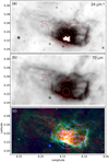 |
Fig. 4 Radio-continuum emission of G008.14+00.23. The Spitzer 24 μm (saturated in the centre) image (panel a) and the Herschel 70 μm image (panel b) over-plotted with 1.4 GHz contours from the NVSS survey (contour levels of 0.01, 0.05, 0.1, 0.5, 1.0, 1.5, 1.25, and 1.5 Jy beam−1). Panel c: colour composite image; red highlights the radio emission at 20 cm from MAGPIS survey (in logarithmic units), green shows the 8 μm emission, and blue shows the unsharp 70 μm emission (tohighlight the borders of the ionised lobes). The white contours indicate the NVSS radio emission (contour levels of 0.1, 0.5, and 1.0 Jy beam−1). |
3.2.3 The ionised lobes
The shape and extent of the lobes depend on the structure of the neutral medium surrounding the dense parental structure. We can trace the lobes using 8.0 μm emission, which borders the IFs. For most bipolar nebulae, the two lobes are of unequal size, which could be due to the combinationof the difference in the density of the medium located on each side of the parental filament and projection effects. The lobes can be characterised as being: i) small and closed (ionisation bounded) if expanding in a high-density medium, or ii) large if expanding in a low-density medium. It may even be open if the density of the surrounding medium is low, as in G010.32–00.15 (Paper I, Figs. 11 and 12).
Sometimes, we see several lobes of different sizes and/or orientations on the same side of the parental filament. We assume this is due to the fact that the IF expands more rapidly in some low-density channels, although we cannot ignore the possibility of a burst of ionisation waves from the central massive stars. One example is G008.14+00.23, which has one small closed lobe and one larger faint lobe on the same side. Some regions show distorted lobes when the IF limiting the lobe meets apre-existing dense condensation during its expansion; see for example Sh 201 of Deharveng et al. (2012) and its analogue in G342.07+00.42 (southern lobe, Fig. A.1) or G316.80–00.05 (southern lobe, Fig. B.1).
The dust in the PDRs bordering the ionised lobes is warm; generally warmer than 20 K and as high as 22–23 K. The G008.14+ 00.23 field illustrates this point as a dust temperature contour level of 20.75 K follows the border of the large northern lobe (Fig. 5). The G316.80–00.05 field offers another example (Fig. B.3). Another characteristic of all our regions is that the warm dust is found in zones emitting at 8.0 μm (e.g. see Fig. B.3c or Fig. F.5c).
Sometimes the column density maps show the presence of molecular material surrounding the ionised lobes. Compared to the parental filaments, the column density is not usually high in these structures, in the range 1–3 × 1022 cm−2 (background subtracted).This is observed for example around the two small lobes of G008.14+00.23, around the bottom lobe of G049.99–00.13, and around the western lobe of G320.25+00.44. The best example, however, is found around the eastern lobe of G338.93–00.06 (Fig. D.3). We suggest that we are dealing with neutral material collected during the expansion of the lobes.
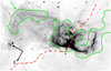 |
Fig. 5 Large northern lobe of G008.14+00.23. The image isof Spitzer 8.0 μm data; the emission of the northern lobe has been enhanced using a logarithmic scaling. The green contour corresponds to a dust temperature of 20.75 K; it follows the PDR bordering the northern lobe (green arrow). The dashed red curve shows the position of the parental filament. |
3.3 The global nature of central stars, YSOs, and clumps
Figure 3 gives a schematic of the various sources observed in the vicinity of the bipolar H II regions: the exciting star or cluster, YSOs, and clumps. Below we describe the global nature and properties of such sources.
3.3.1 The exciting central star or cluster
The identification of the stellar sources (e.g. the exciting star or cluster) allows for an estimate of the distance to the H II region; G010.32–00.15 from Paper I illustrates this point. Prior to our study, the distance to this region was very uncertain, in the range of 2–19 kpc for kinematic distances. The spectral type of the exciting star is known, determined by Bik et al. (2005). UKIDSS images of the region show the exciting cluster. Using NIR data of the exciting cluster we estimated its distance to be 1.75 kpc, close to the near kinematic distance.
The exciting star or cluster is expected to lie at the centre of the H II region. The region G319.88+00.79 presents an exemplary case of a central exciting cluster (Fig. 5 in Paper I); the cluster lies at the exact centre of the waist, at the centre of the elliptical ring. In this work, we have identified the most-likely exciting star (except for G316.80–00.05) in the central regions of the bipolar nebulae; in most cases, we do not see a cluster around them. In bipolar bubbles, this central region is generally found in the direction of the parental filament, and therefore may be strongly affected by extinction. This is one of the possible reasons for not being able to identify the exciting cluster in most of the H II regions. For example, we searched for the exciting cluster of G320.25+00.14 and G316.80–00.05, but we were not able to conclusively identify them. Similarly, we do not see any stellar cluster in the central region of G004.40+00.11 and G008.14+00.23.
3.3.2 The evolutionary status of the YSOs
We use two different indicators to identify YSOs: GLIMPSE [3.6]–[4.5] vs. [5.8]–[8.0] colours and [8]–[24] colours. As underlined in Sect. 2.4, the GLIMPSE [3.6]–[4.5] vs. [5.8]–[8.0] diagram is sensitive to the extinction, whereas the [8]–[24] colour is less sensitive. In Fig. 6, we compare the results obtained with the above two indicators. We are interested only in sources located in or close to the zone defined for Class I sources in the GLIMPSE colour–colour diagrams. Figure 6 shows the results obtained for 84 GLIMPSE Class-I sources with [8]–[24] colour, located in the fields of G010.32–00.14, G018.66–00.06, G049.99–00.13, G316.80–00.05, G319.88 + 00.79, G320.25 + 00.44, G338.93–00.06, and G339.59–00.12. Based on their [8]–[24] colours, they have been classified into different evolutionary stages and are shown in different colours in Fig. 6. The small red dots in the Class I zone are for sources of unknown nature; they have no 24 μm measurements, because they are either saturated or not detected at 24 μm. Of the IRAC-identified Class I YSOs that have 24 μm detections, we find that 28 are Class I (the two indicators agree), 25 are flat-spectrum, and 12 are Class II based on their [8]–[24] colours. This analysis shows the difficulty in disentangling Class I and Class II YSOs based on GLIMPSE data only, and thus the need for high-resolution longer-wavelength observations. Nonetheless, we can say that roughly 80% of the IRAC-classified Class I sources should be protostellar (i.e. Class I and flat-spectrum). The lifetime of Class I and flat-spectrum sources are of the order 105 yr; therefore, the presence of such sources suggests recent star formation activity in the region.
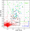 |
Fig. 6 Identified Class I YSOs in the field of bipolar nebulae, using two indicators. The underlying diagram is that ofthe region G316.80–00.05 (Fig. B.9), although the diagram of any other region could have been used. The colours give the nature of these sources according to their [8]–[24] colours. Green, blue, and black circles identify Class I, flat-spectrum, and Class II YSOs, respectively. Black “X” sources are for probable evolved stars. Small red dots are for sources of unknown nature because their 24 μm magnitude is unknown. The extinction law is that of Indebetouw et al. (2005). |
3.3.3 Location and properties of molecular clumps
Massive clumps are always present at the waist of the nebulae; they are part of the parental structure. The clumps found adjacent to the ionised regions are always the most massive, compact, and dense structures in the vicinity. We do not compare their peak column densities as these values depend on their angular sizes as compared to the resolution of the 250 μm observations. We do, however, compare their mass and mean volume densities of the central regions assuming that shape of the clumps is Gaussian in nature, and therefore their total mass is twice that of the central regions (see discussion in Sect. 2.2).
Figure 7 shows the masses of these clumps, which lie in the range 200M⊙–1400M⊙. We observe no relationship between the mass of the clumps and ionising source of the central nebulae. We suggest instead that the observed mass of the clumps strongly depends on the density and structure of the parental clouds, star-formation activity within the clumps, and/or the age of the central bipolar nebulae (if formed by collect-and-collapse-like process, then older sources are expected to collect more material; see discussion in Deharveng et al. 2010).
Figure 8 displays the mean density of the central regions of the clumps. The density can be as high as a few 106 cm−3. Globally, the density of clumps containing a luminous source (massive YSOs or ultra-compact (UC) H II regions) is higher than that of clumps devoid of luminous sources. It therefore seems that for these regions massive stars form in dense clumps rather than in massive ones.
Infrareddark clouds (IRDCs) are often described as the locations where star formation occurs. Based on Spitzer 8 μm opacity maps, Peretto & Fuller (2009) identified over 50 000 single-peaked IRDC fragments in our Galaxy, in the region of Galactic longitude and latitude 10° < |l| < 65° and |b| < 1°. Many of the massive and dense clumps inside which massive stars are forming are not reported as IRDC fragments by Peretto & Fuller (2009). Such clumps are not seen in absorption at Spitzer wavelengths due to their locations near to H II regions and their PDRs, and therefore they are hidden by the bright emission of the PDRs. Many examples can be found:
In the G010.32–00.14 (Paper I) field, three massive clumps (C1, C2, and C3 of mass 180, 223, and 330 M⊙, respectively) lie at the waist of nebula and are not IRDCs; they contain MYSOs (maser sources) of high luminosity (>1600 L⊙).
In the G320.25+00.44 field (Appendix C), the most massive (~280 M⊙) clump, C1, has not been identified as an IRDC despite being a strong absorption feature at 8.0 μm. It contains a source with a luminosity ~1700L⊙.
-
In the G339.58–00.12 field (Appendix E), two massive clumps (C1 of mass 550M⊙ and C2 of mass 360M⊙; see Fig. E.4) are located at the waist of the nebula. C1 contains a MYSO of luminosity ~2400L⊙ which is not an IRDC, and the IRDC detected in the vicinity of C2 (which contains a young cluster of 15 000L⊙) lies far from the column density peak.
We suggest in the field of H II regions that Spitzer-based IRDC fragments are not likely to be the best sites to search for massive star formation.
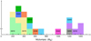 |
Fig. 7 Mass of the clumps associated with bipolar nebulae, observed either around their waists or along the parental filaments. |
4 Star formation near bipolar H II regions
This section discusses various components of the recent star-formation observed around the bipolar H II regions, and the possible existence of triggered star-formation in these regions.
4.1 Bright-rimmed clumps at the waist
Clumps located at the waist of bipolar nebulae are often surrounded by bright rims (BRs) that are bright at 8.0 μm. The BRs are observed on the clump-side adjacent to the ionised region. A Class I YSO is often located inside the clump, not towards its centre, but just behind the bright rim and very close to it. We describe two such cases are as follows. The best example is from the bipolar nebula G316.80–00.05 (Fig. B.7). Two clumps, C1 and C2, are located close to the eastern waist of the nebula. The C1 clump (mass ~ 1360M⊙, density ~ 7.4 × 105 cm−3) is bordered by a BR on its face turned towards the ionised region. This BR is also a dense ionised layer (it displays arc-like radio emission). Behind the BR, at ~0.03 pc in projection, lies a hydroxyl (OH), water (H2O), and methanol (CH3OH) maser that is also coincident with an EGO with jets. This is therefore a Class I YSO. The luminosity of this source is estimated to be ~26 000L⊙. The resolution of the radio emission does not allow us to separate the emission of the BR and that of the massive YSOs forming nearby.
The bipolar nebula G004.40+00.11 is another example that has bright rim clumps. Two clumps, C1 and C2, are located at the northern extremity ofthe waist. Each clump contains a YSO (see Fig. 9). The C2 clump is located adjacent to the H II region. It is warm and surrounded by a bright rim. Wide-field Infrared Survey Explorer (WISE; Wright et al. 2010) photometry suggests that the source embedded in C2 is a Class I YSO. The 4.5 μm image shows the presence of faint extended emission close to the YSO; we suggest that it is likely due an outflow activity such as those found in EGOs (e.g. Cyganowski et al. 2008). It lies very close to the bright rim ( ~2.′′6 in projection).
In some other regions, the YSO is rather far from the BR, but not in the very centre of the clump. One example is the G010.32–00.14 bipolar H II region (Paper I, Fig. 23). The central clumps, C2 and C3, are bordered on their side facing the exciting cluster by BRs observed both at 8.0 μm and at radio wavelengths (in the MAGPIS survey images). They contain massive young sources. For example, C1 contains a massive Class I YSO of high luminosity (4600L⊙; associated with a methanol maser), while C2 contains a UC H II region. These two sources do not lie at the centre of the clumps. Another example is the G338.93–00.06 region, which has an elliptic waist (Appendix D) with a bright clump (C1: mass ~275M⊙, density ~2.7 × 106 cm−3) bordered bya BR. Behind the BR, at about 0.1 pc in projection (at equal distance between the BR and the column density peak) lies an IR source associated with a methanol maser. This source is bright at 70 μm, with a luminosity of ~4500 L⊙.
 |
Fig. 8 Mean volume density of the clumps associated with bipolar nebulae, observed either around their waists or along the parental filaments. The black circles indicate clumps containing a source more luminous than 1000L⊙. The red lineon the low-density side indicates the range of densities estimated for the parental structures. |
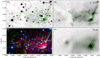 |
Fig. 9 Star formation in two clumps located at the waist of G004.40+00.11. The stellar content of the clumps is shown by 4.5 μm (panel a), 8.0 μm (panel b), and 70 μm (panel c) images. The over-plotted red contours are of column density (levels of 1.5, 1.0, 0.75, 0.5, 0.25 × 1023 cm−2) and the green contours are of 70 μm emission (levels of 20 000, 15 000, 10 000 MJy sr−1). Panel d: composite colour image with 70 μm emission in red, an unsharp image of the 8.0 μm emission highlighting the bright rim bordering clump C2 in green, and 4.5 μm emission in blue. The orange arrows point to the two YSOs emitting at 70 μm. The green contours are of 70 μm emission. |
4.2 Possible second-generation young clusters
Young clusters (small groups of Class I YSOs or IR point sources as opposed to isolated point sources) are observed in the following two regions. Firstly, the G339.59–00.12 field (Appendix E). Two massive and dense clumps, C1 and C2, are observed at the waist of the nebula (see Fig. E.4). Massive-star formation is observed in each of them. The C1 clump (mass ~ 550M⊙, density ~6.2 × 105 cm−3; Fig. 10) contains a small group of Class I and flat-spectrum YSOs (at least 4 Class I), an EGO, and a methanol maser. Secondly, the G342.07+00.42 field (Appendix F). Two massive and dense clumps, C1 and C2, are observed at the waist of the nebula (see Fig. F.4). The C1 clump (mass ~ 1030M⊙, density ~ 2.9 × 105 cm−3) lies on the west side of the waist. On VISTA images, a tight cluster seems to be embedded in C1 (Fig. 11). The clump contains a UC H II region lying only ~ 6′′ from the massive star of the cluster.
Since UC H II regions and masers trace very early phases ( ≤105 yr) of star formation. We suggest that these clusters are likely second-generation clusters of the field.
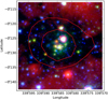 |
Fig. 10 Colour composite image showing the second-generation cluster of G339.59–00.12. The image is made with Spitzer 8.0 μm (red), 4.5 μm (green), and VISTA Ks (blue) data. The red contours are for column densities of 0.5 × 10²³ and 1.0 × 1023 cm−2. |
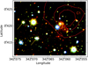 |
Fig. 11 Colour composite image showing the second-generation cluster of G342.07+00.42. The image ismade with VISTA J- (blue), H- (green), and K-band (red) images. The red contours are for column densities of 0.5 × 10²³, 1.0 × 10²³, and 1.5 × 1023 cm−2. The two orange arrows point to probable candidate exciting stars. |
4.3 Small diffuse regions
Small diffuseregions of extended 8.0, 24, and 70 μm emission areoften observed in the vicinity of bipolar nebulae. These extended regions are much smaller in size compared to the bipolar H II regions (e.g. 0.25 vs. 3.8 pc for region D in the field of G316.80–0.05). A star is often present in the centre of these regions. Based on these stars’ brightnesses and the lack of detected free-free emission from ionised gas, the stars may be of spectral type B. For example, in the field of G049.99–00.13 (Appendix A), three such regions are present. Two regions are located along the parental filament, in a condensation adjacent to the ionised region, and behind a bright rim; they are therefore likely associated with the bipolar nebula. In G339.59–00.12 (Appendix E), four small regions are present. Two of them contains stars. In the field of G316.80–00.05 (Appendix B), seven such regions are observed.
We suggest that these presumed B-type stars heat the dust and excite PAHs in their surroundings. We would require deep high-resolution radio observations to determine if the stars are massive enough to ionise their surroundings and form UC H II regions. Only in the case of G010.32–00.14 (Paper I; MAGPIS observations) we know the presence of a UC H II region.
We have no information on the evolutionary status of most of these regions. At longer wavelengths these sources are extended, and therefore we cannot conclusively say whether they are of the same generation as the exciting stars of the bipolar nebulae or if they represent second-generation massive stars. Only in the case of the UC H II region in G010.32–00.14 we suggest that we are looking at a second-generation massive source, as it is embedded inside a clump compressed by the adjacent central nebula. Spectroscopic observations would reveal the true nature of these sources.
4.4 Triggered star formation
In the studied regions, several observational signatures point to star formation triggered by the central expanding bipolar H II regions.
The most massive clumps in all our fields are without exception adjacent to the central ionised region. We cannot exclude that a few of them were pre-existing along the parental filament or in the parental sheet, but we regard it as probable that all of them were pre-existing as very low. How did these clumps form? We suggest that they formed from collected material as the ionised region expanded into the dense material of the parental filament or sheet. The morphology of the G010.32–00.14 complex (Paper I) is consistent with this interpretation, as there are five massive clumps surrounding the waist of the bipolar nebula. Again, we regard the probability of finding five pre-existing clumps surrounding an H II region and reached by the IF at the same time as very low. A similar situation is observed in G338.93–00.06 where four condensations are distributed along the waist of the nebula (Fig. D.3).
We know that a very early phase of star formation is at work in these clumps because Class 0/I sources, often associated with class II methanol masers, are detected in the direction of these clumps. In a few cases, we observe these sources close to the IF. This suggests that they form in the high-density compressed layer bordering the IF. High-angular-resolution molecular observations would allow us to better determine the morphology of the clumps in the vicinity of the IF.
We note that this type of star formation, that we believe was triggered by the expansion of central H II region, leads to the formation of luminous (and therefore probably massive) sources (see Fig. 8). One extreme example is the UC H II region embedded in clump C3 in the G010.32–00.14 field. Another extreme case is the source embedded in the C1 clump in the G316.804–400.05 field, which has a luminosity of ~26 000 L⊙ and is observed very close to the IF. The central bipolar H II regions in these two cases have the highest excitation degree of the sample (they are ionised by O4–O6 stars).
In a few cases, we observe collected material surrounding the lobes, but no stars are forming there3. The column density of this material is rather low, of the order of a few 1021 cm−2, much lower than that of the parental filamentary structure. This is probably the reason why no star formation is observed there.
We also observe star formation in pre-existing clumps reached by the IF limiting the lobes (C6 on the border of the bottom lobe in G010.32–00.14 and C5 on the border of the right lobe in G338.93–00.06; each shows star formation presently at work). In these cases, we do not know if star formation has been triggered by the compression of the clump by the high pressure ionised gas, or if star formation was already at work before the compression.
5 Conclusions
In this work, we studied six bipolar H II regions at NIR, mid-infrared (MIR), FIR, and radio wavelengths to determine their morphologies, parental cloud structures, and their impact on star formation in their vicinities. Our main conclusions are:
- 1.
Massive clumps are present at the waist of bipolar H II regions, adjacent to the ionised gas in all cases. They are massive, with several hundred solar masses in their central regions. High densities are found there, higher than 105 cm−3, and up to several 106 cm−3.
- 2.
Massive Class I YSOs are frequently associated with masers in these clumps. The more luminous ones lie in the densest clumps. Some clumps also contain small clusters of Class I YSOs.
- 3.
The massive YSOs are generally not located – in projection – at the centres of the clumps, but instead are found near the bright rims bordering the clumps on their faces towards the ionised gas. In some cases, they lie very close to the IF, probably in or close to the layer of compressed material bordering the IF.
- 4.
Star formation also occurs in some pre-existing condensations reached by the IF during the expansion of the ionised lobes.
- 5.
Points 1, 2, and 3 show that star formation has likely been triggered by the expansion of the central bipolar H II regions. As most of the massive YSOs are found at the waist of bipolar regions, this implies that recent star formation is mainly occurring in the material collected from the dense parental structures and not from the lower-density surrounding medium (therefore from material collected in the dense parental structure, and not in the material collected around the lobes).
We have covered the area located between longitude –60° and +60°, latitude –1° and +1°. This area contains about 1377 large bubble H II regions (Simpson et al. 2012). By eye, we have only identified 16 bipolar H II regions; even if this number is underestimated by a large factor (mainly because we identify mostly bipolar H II regions seen edge-on) it is several hundred times smaller than the number of bubble H II regions identified by Simpson et al. (2012). This suggests that most of the bubble H II regions in our Galaxy are probably not formed in two-dimensional, flat or sheet-like clouds.
The cloud structure that is at the origin of the bubble H II regions remains to be understood. Modelling and numerical simulationsof bipolar H II regions are missing, although a very recent model by Whitworth et al. (2018) suggests that bipolar H II regions can be created at the interface resulting from collisions between two clouds. More high-resolution simulations following the formation and evolution of an H II region excited by a massive star formed in a two-dimensional parental structure or inside a filament would shed light on their origin.
We also need to follow the formation of dense and massive clumps at the waist of the nebula, and the formation of massive sources inside these clumps. High-resolution molecular observations of clumps with ALMA may help to understand exactly where star formation occurs, in the compressed layer adjacent to the IF as these first observations seem to indicate, or more embedded inside the clump.
Acknowledgements
We thank the anonymous referee for helpful and constructive comments. The authors would first like to thank the Herschel Hi-GAL team for their continuing work on the survey. Observations were obtained with the Herschel-PACS and Herschel-SPIRE photometers. PACS was developed by a consortium of institutes led by MPE (Germany), including UVIE (Austria); KU Leuven, CSL, IMEC (Belgium); CEA, LAM (France); MPIA (Germany); INAF-IFSI/OAA/OAP/OAT, LENS, SISSA (Italy); IAC (Spain). This development was supported by the funding agencies BMVIT (Austria), ESA-PRODEX (Belgium), CEA/CNES (France), DLR (Germany), ASI/INAF (Italy), and CICYT/MCYT (Spain). SPIRE has been developed by a consortium of institutes led by Cardiff Univ. (UK) and including Univ. Lethbridge (Canada); NAOC (PR China); CEA, LAM (France); IFSI, Univ. Padua (Italy); IAC (Spain); Stockholm Observatory (Sweden); Imperial College London, RAL, UCL-MSSL, UKATC, Univ. Sussex (UK); Caltech, JPL, NHSC, Univ. Colorado (USA). This development was supported by national funding agencies: CSA (Canada); NAOC (PR China); CEA, CNES, CNRS (France); ASI (Italy); MCINN (Spain); SNSB (Sweden); STFC and UKSA (UK); and NASA (USA). This paper uses data form VISTA Variables in the Vía Láctea survey, obtained with VIRCAM/VISTA at the ESO Paranal Observatory. The VVV Survey is supported by BASAL Center for Astrophysics and Associated Technologies CATA PFB-06, by the Ministry of Economy, Development, and Tourism’s Millennium Science Initiative through grant IC12009, awarded to The Millennium Institute of Astrophysics (MAS). This publication makes use of data from The UKIRT Infrared Deep Sky Survey or UKIDSS which is a next generation near-infrared sky survey using the wide field camera (WFCAM) on the United Kingdom Infrared Telescope on Mauna Kea. This publication also made use of data products from the Two Micron All Sky Survey (a joint project of the University of Massachusetts and the Infrared Processing and Analysis Center / California Institute of Technology, funded by NASA and NSF. This paper also uses data observationsmade with the Spitzer Space Telescope (operated by the Jet Propulsion Laboratory, California Institute of Technology under a contract with NASA). We thank the French Space Agency (CNES) for financial support.
Appendix A G049.99–00.13
The H II region G49.99–00.13 is a small bipolar nebula (Fig. A.1). Two lobes are visible in the 8 μm, 24 μm, and 70 μm maps. One lobe is small ( ~1.5′) and closed, whereas the other is large ( ~2.3′) and relatively open. A filament is present, seen in absorption at 8 μm, and in emission at all Herschel-SPIRE wavelengths. The filament is perpendicular to the two lobes. A circular region of extended 24 μm emission is present in the centre of the nebula.
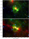 |
Fig. A.1 Bipolar nebula G049.99–00.13. Panel a: composite colour image with the Spitzer 24 μm, 8.0 μm, and 4.5 μm emission in red, green, and blue, respectively. Panel b: the red channel is now the Herschel column density map showing the parentalfilament. |
No Hα emission is detected in the optical images, but radio-continuum emission is observed in the NVSS and VGPS maps. The radio continuum flux density peaks in the direction of the region of extended 24 μm emission.
An IRAS source, IRAS 19214 + 1458 (coordinates: l = 49. °9973, b = –00. °1252), is spatially coincident with the H II region. It lies near the centre of the region of extended 24 μm emission.
A.1 Distance and exciting cluster
The integrated VGPS flux at 1.4 GHz is 460 mJy, and the flux at 9 GHz is 407 mJy (Anderson et al. 2011). High-resolution VLA observations found an integrated flux density of 238 mJy at 5 GHz (Hughes & MacLeod 1994). We believe because of the missing short-spacing of the VLA data, the flux density is a lower limit.
Anderson et al. (2011) found two recombination line velocities toward the region, at 38.5 km s−1 and 73.2 km s−1. Anderson et al. (2015) determined that the 38.5 km s−1 velocity is the correct one for the region and the other one is from diffuse ionised gas along the line of sight. The kinematic distance to the region is therefore 2.99 kpc or 7.94 kpc. As an HI absorption line is present at 55 km s−1, Anderson et al. (2015) prefer the far distance of 7.94 kpc, which we adopt in the following. Due to the complicated velocity field in this region, this distance is somewhat uncertain4.
Using the radio flux at 5 GHz and an electron temperature of 8000 K for the H II region, we estimate a ionising photon flux of ~2.70 × 1048 s−1 for distance 7.94 kpc. This corresponds to the output from an O7.5V star.
As mentioned previously, the peak of the radio continuum emission from the VGPS survey coincides with the peak of the 24 μm. Several stars are observed in this direction in the NIR, as shown by Fig. A.2. They do not form a tight cluster, but a few stars are possibly highly reddened by an overlapping foreground dust clump (i.e. the C2 clump discussed in Appendix A.2, whose peak column density is ~4.5 × 1022 cm−2).
Kang et al. (2009) used Spitzer data to look for candidate YSOs of W51 including G049.99–00.13. They propose five candidate YSOs in the vicinity of G049.99–00.13. They are tabulated as sources #1 to #5 in Table A.1 along with their coordinates and photometric magnitudes. Kang et al. (2009) suggest that the faintest one at Spitzer-IRAC wavelengths, G049.9977–00.1261 (i.e. the source #4 of the Table. A.1), is a stage 0/I YSO on the basis of its strong 24 μm emission. We doubt this classification. G049.9977–00.1261 lies in the direction of the central ionised region, so we believe that the background emission from warm dust has contaminated the measurement of the 24 μm flux. This source is almost undetectable at 8.0 μm but is detected at all other Spitzer-IRAC wavelengths and in the NIR.
We propose that G049.9977–00.1261 is instead the main exciting star of the G049.99–00.13 H II region; we call it “ex1” (see Fig. A.2 for the location of the star and Table A.1 for its photometric magnitudes). Its JHKs magnitudes (from the UKIDSS catalogue) point to an O7V star affected by a visual extinction of ~15.1 mag if lying at 7.94 kpc. This agrees with the radio flux of the H II region. A nearby star that we called “ex2” (see Table A.1), has the ability to participate in the ionisation of the nebula as it seems to be an O9.5–B0V star affected by 10.8 mag of visual extinction. However, the UKIDSS JHKs images show that this star is double (see the insert zoomed image of Fig. A.2), with two components of similar brightness separated by about 0.′′9 (UKIDSS catalogue has a single measurement for both stars and the coordinates of the measurement lie between the stars); this points to two early B stars.
A.2 Dust temperature, column density, and molecular clumps
Figure A.3 presents the temperature map of the region. The parental filament is cold, with dust temperatures in the range 15 K–16 K. The PDRs surrounding the ionised gas contain warmer dust, everywhere higher than 18.5 K; the maximum temperature is 19.3 K.
Infrared sources in the field of G049.99–00.13.
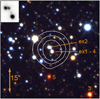 |
Fig. A.2 JHKs UKIDSS colour composite image of the centre of the nebula; Ks is red, H is green, and J is blue. The white contours indicate the centre of the extended 24 μm emission (levels of 400, 500, and 600 MJy sr−1). The two candidate exciting stars, ex1 and ex2, are identified, as well as two other YSO candidates, #3 and #5, identified by Kang et al. (2009). The insert is an enlargement of the UKIDSS Ks image of ex1 and ex2. |
Molecular clumps associated with G049.99–00.13.
Figure A.4 presents the column density map. In the filament, far from the H II region (e.g. at l = 50.1°, b = –0.10°), the column density is in the range 1.5–2 × 1022 cm−2. Three brightclumps (labelled as C1, C2, and C3 in the figure) are present at the waist of G049.99–00.13, along the parental filament with column density ~2.8 × 1022 cm−2 in C3, and ~5.1 × 1022 cm−2 in C2 and C1. The minimum column density is 7 × 1021 cm−2 in the field of Fig. A.4, therefore in the region surrounding G049.99– 00.13.
The SPIRE images show cold dust emission surrounding the two lobes. This emission is faint, with column densities of the order of 1.5 × 1022 cm−2 or even less;we suggest that this emission traces material collected around the ionised region during its expansion.
As discussed above, three bright clumps are present at the waist of G049.99–00.13, along the parental filament. We summaries the clump parameters in Table A.2. These parameters refer to the central region of the clumps, enclosed by apertures following the level at half the peak column density, after subtracting a background column density value. As can be seen from the table, the clumps are massive, containing several hundred solar masses in their central regions. We did not consider these regions as “cores”5 as they are too large (more than 0.3 pc); G049.99–00.13 lies too far away for Herschel to resolve cores. The mean volume density in the central regions is of the order of a few 104 cm−3 in C1 and C2, and less ( ~6 × 104 cm−3) in C3. Since these clumps are cold; we suggest that they lie in front of the ionised gas along the line of sight, and therefore we do not see their face adjacent to the ionised region.
A.3 Infrared dark clouds
Two IRDC fragments are detected by Peretto & Fuller (2009) in the vicinity of the nebula. The locations of these clouds are shown in Fig. A.5. As can be seen from the figure, one of them corresponds to a real structure and the other corresponds to a low-brightness region close to periphery of the western lobe. The compact massive clumps, C1 and C2, which are strong absorption features at 8.0 μm, have not been identified as IRDC fragments.
A.4 Young stellar objects and star formation
Here, we examine the YSOs identified by Kang et al. and then use them to discuss the star formation activity. These sources are identified in Fig. A.6:
Kang et al.’s source G049.9977–00.1261 (i.e. source #4 or ex1) lies at the very centre of the central extended 24 μm emissionregion, as shown by Fig. A.2. We suggest that this source is the main exciting star of the bipolar nebula (see preceding section).
Kang et al.’s YSOs G049.9842–00.1502, G049.9899–00.1413, G049.9914–00.1333, and G049.9982–00.1303 1, respectively, correspond to our sources #1, #2, #3, and #5 in Table A.1. We agree with their classification as YSOs.
YSO #1 lies on the border of the bottom lobe, away from the waist of the bipolar nebula. Its association with the nebula istherefore uncertain. It has no detectable 70 μm counterpart. Kang et al. classify it as a flat-spectrum source, and we agree with this classification.
YSO #2 lies in the direction of the bright rim bordering the condensation C1 at the waist of the nebula. Based on its location, we believe it is most probably associated with the bipolar nebula. It lies in a region of extended 24 μm emission(from the PDR); as a consequence its [24] magnitude can be uncertain. It lies ~5′′ away from a 70 μm source (CuTEXflux ~12.7 Jy). According to its [8]–[24] colour, we classify it as a Class II YSO.
YSOs #3 and #5 lie at the waist of the nebula, along the parental filament, in regions of high column density (#3 lies between C1 and C2, #5 embedded in C2). Kang et al. classify #3 as a flat-spectrum source, and we agree with this classification. YSO #5 is a Class I source according to its [8]–[24] colour (in agreement with Kang et al.). Both #3 and #5 sources have compact 70 μm counterparts; their 70 μm fluxes point respectively to luminosities of ~1150L⊙ and ~2300L⊙.
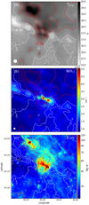 |
Fig. A.3 Dust temperature in the field of G049.99–00.13. The red contours are for dust temperatures of 17.5 K, 18 K, 18.5 K, and 19 K. The white ones are for 15.5 K, 16 K, 16.5 K, and 17 K. The contours are superimposed on the dust temperature map (panel a), the column density map (panel b), and the 8.0 μm image (panel c). |
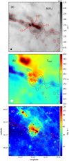 |
Fig. A.4 Column density in the field of G049.99–00.13. The red contours correspond to levels of 1.25, 1.5, 2, 3, and 4 × 1022 cm−2. They are superimposed on the column density map (panel a), the temperature map (panel b), and the 8.0 μm image (panel c). |
Small diffuse regions in the field of G049.99–00.13.
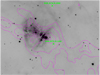 |
Fig. A.5 Location of IRDC fragments in the field of G049.9977–00.1261. The underlying image is the Spitzer 8.0 μm emission. The contours are from the column density map and are at same level as in Fig. A.4. |
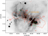 |
Fig. A.6 Spatial distribution of various sources in the field of G049.9977–00.1261 that are discussed in the text. The underlying grey image is the Spitzer 8.0 μm image. The column density contours are in red (levels of 2, 3, 4, and 5 × 1022 cm−2). The diffuse regions are identified in green, the YSOs in red, and the exciting stars in orange. |
Figure 2 displays three unsharp-masked images of G049.99–00.13. They allow the detection of all the point-sources present in the vicinity of the nebula. The figure shows very clearly that all these sources (except the source #1) are aligned and located inside or on the border of condensations present along the parental filament and adjacent to the ionised gas. Star formation has been and is presently at work at the waist of the G049.99–00.13 bipolar nebula.
A.5 Small regions of extended diffuse IR emission
Three sources observed at 8.0, 24, and 70 μm in the vicinity of G049.9977–00.1261 appear to be diffuse and non-stellar; they are the regions A, B, and C, identified in Fig. A.6. A star is present in the centre of each region. Their UKIDSS JHKs magnitudes are given in Table A.3. We suggest that regions A and B are associated with the complex as they lie in the centre of clump C1. The association of diffuse region C is more uncertain. Assuming a distance of 7.94 kpc, the UKIDSS data are consistent with the central star of region A being of spectral type B0.5V affected by a visual extinction of 23.4 mag, the central star of region B a B1V star affected by a visual extinction of 23.5 mag, and the central star of region C a later B-type star affected by an extinction of ~14.2 mag. None of these small and faint regions are detected in the VGPS data.
We find, compared to the exciting star of the nebula, that the massive stars of the regions A, B, and C are surrounded by diffuse yet relatively compact emission at 24 and 70 μm, and the regions are embedded in cold clumps (at least A and B); therefore these embedded stars are likely younger than the central exciting star. However, in the absence of spectroscopic information we cannot be very sure about their true evolutionary status.
Appendix B G316.80–00.05, or S109, S110, and S111
The group of three bubbles (S109, S110, and S111) forms the bipolar nebula G316.80–00.05 (Fig. B.1); their morphology is listed as “TP” in the Churchwell et al. (2006) catalogue6. The parental filament of the nebula is seen in absorption in the visible, NIR, and at Spitzer-GLIMPSE wavelengths (Fig. B.1a), whereas it is seen in emission at Herschel-SPIRE wavelengths (Fig. B.1b). This filament extends over 17′ ( ~14 pc for a distance of 2.8 kpc, justified later on). The S110 bubble is the northern lobe, which extends perpendicular to the filament. S109 and S111 form the southern lobe with a complicated morphology. In the north, we see two lobes, a small bright one corresponding to the S110 bubble, and a faint, extended, closed one (extending up to 10′ or 9 pc, from the centre of the nebula). The southern lobe also shows filaments extending south-west (up to 12′ or 10 pc from the centre). The morphology of the lobes is complicated, probably due to the presence of inhomogeneous dense interacting structures distorting the IF and also ionising photons in some directions, through holes, reaching far away regions.
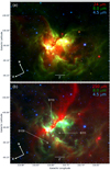 |
Fig. B.1 Bipolar nebula G316.80–00.05. Panel a: composite colour image of the G316.790-0.045 complex: red, green, and blue indicatethe Spitzer 24 μm, 8.0 μm, and 4.5 μm data, respectively (the 24 μm emission is saturated in the centre). Panel b: composite colour image of the complex: red is for the Herschel 250 μm emission showing the cold filament at the waist of the nebula, green is for the 8 μm PAH emission, blue is for the 4.5 μm stellar emission. The three bubbles listed in the (Churchwell et al. 2006) catalogue are identified. |
The bipolar H II region is faintly visible in the Hα superCOSMOS image, but we see diffuse emission of the ionised gas in the northern (S110) and southern lobes (S111, and also bright emission south of S111). Figure B.2 shows the radio continuum emission of the central region at 843 MHz (SUMSS; resolution 43′′ × 50′′) superimposed on the Hi-GAL 70 μm image. The contour level at 1 Jy beam−1 follows the limits of the saturated 24 μm zone. Figure B.2 shows that the peak of the radio emission lies between the C1 and C2 clumps (clumps are discussed in Appendix B.2). There is also an extension of the radio emission in the direction of a compact 8.0 μm to 70 μm emission region (discussed in Appendix B.5).
An IRAS source, IRAS 14416–5937 (coordinates: l = 316. °814, b = –000. °58), lies in the direction of the nebula. It has been studied in the IR bands by Vig et al. (2007). We discuss their results in Appendix B.2.
B.1 Distanceand exciting star
A mean velocity of the ionised gas at optical bands is V (Hα) = − 38 km s−1 (Georgelin et al. 1987), in agreement with the velocity measured using radio recombination lines: V (H109α) = –36.1 ± 1.1 km s−1 (Wilson et al. 1970b), V (H76α) = –38.1 ± 0.1 km s−1 (Mc Gee et al. 1981).
The distance of G316.8–0.1 has been discussed by Shaver et al. (1981). Based on kinematic and IR photometric arguments, the near kinematic distance is favoured by these authors. More recently, Busfield et al. (2006) resolved the distance ambiguity using HI self-absorption observations. According to them, G316.8–0.1 lies at a near kinematic distance of 2.8 ± 0.6 kpc.
The ionised region has been observed in radio continuum emission. Its flux is 32 ± 5 Jy at 1415 MHz (Shaver et al. 1981), 30.04 Jy at 4.85 GHz (Kuchar & Clark 1997), and 37.5 Jy at 843 MHz (Vig et al. 2007). Assuming a distance of 2.8 kpc and an electron temperature of 8000 K, these fluxes correspond to an ionising photon flux of ~2.18 × 1049 photons s−1, and therefore point to an O4–O5V star.
Hα emission is faint in the direction of the H II region, which indicates a high level of extinction. No exciting cluster has been clearly identified around the centre of the nebula, probably as a consequence of the high extinction. The stellar content of the region has been discussed by Vig et al. (2007). They searched for the exciting star of the central H II region among the 2MASS sources lying within the 30% contour of the radio peak at 843 MHz and above the reddening vector of a ZAMS O6 star in the J vs. J − H diagram. They adopted a distance of 2.8 kpc. Six stars were selected by them (the parameters of these stars are given in their table 5). If the distance is 2.8 kpc, all these stars lie clearly above the location of reddened O3 stars. Among these stars, one star (J14452143–594925: l = 316. °800, b = –00. °055) lies in the central area of radio emission seen at 843 MHz (Fig. B.2); it also lies close to the radio emission seen in the high-resolution radio image at 24 GHz (see Fig. B.7), and therefore may be the exciting star of the nebula. However, its SED shows the presence of an envelope (Vig et al. 2007), and thus it could also be a massive YSO with strong IR excess. We cannot therefore conclusively say the reddened O3 star identified by Vig et al. (2007) is the exciting star of the nebula. The column density in this region is ~1023 cm−2 (discussed in Sect. B.2) corresponding to a visual extinction of ~100 mag. Therefore, the non-detection of an exciting star and associated cluster is not surprising in this nebula.
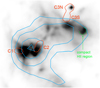 |
Fig. B.2 Central zone of the G316.80–00.05 bipolar H II region. The underlying image shows Hi-GAL 70 μm emission. The blue contours are of SUMSS 843 MHz radio emission (levels of 0.5, 1.0, 2.0, and 3.0 Jy beam−1). The column density contours (in red) show the central area of the C1 to C3 clumps (contour level ~2.0 × 1023 cm−2). |
B.2 Dust temperature, column density, and molecular clumps
Figure B.3a presents the dust temperature map of G316.80–00.05. As can be seen, the parental filament is cold, with dust temperatures lower than 17 K and a minimum at 14.1 K. The PDRs surrounding the ionised gas contain warmer dust, higher than 19 K throughout. The large northern lobe is well-traced by warm dust, in the range 19–20 K (indicated by black arrows in Fig. B.3a). In particular, it shows a good correlation between the warm dust emission ( ≥20 K) and the PAH 8.0 μm emission that comes from the PDRs adjacent to the ionised gas (see Fig. B.3c). In Fig. B.3a one can also see a compact structure (coordinates: l = 316. °753, b = –00. °036) with a muchhigher temperature peaking at 29.2 K. We find this is likely due to the presence of a compact H II region (further discussed in Appendix B.5.)
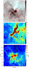 |
Fig. B.3 Dust temperature in the field of G316.80–00.05. The red contours are for temperatures of 19 K, 20 K, 21 K, 23 K, 25 K, and 27 K while the blue ones are for 15 K, 16 K, 17 K, and 18 K. The contours are superimposed on the dust temperature map (panel a), column density map (panel b), and the 8.0 μm image (panel c). The black arrows in the temperature map show the warm (19 K–20 K) PDR surrounding the large northern lobe. |
Figure B.4 shows the column density map of G316.80–00.05. High column densities are observed all along the parental filament, higher than 5 × 1022 cm−2 throughout.High-column-density material ( ≥2 × 1022 cm−2) is also observed around the southern lobe, especially on the borders of the S111 bubble (see Fig. B.4b).
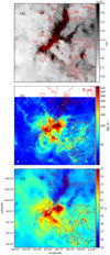 |
Fig. B.4 Column density in the field of G316.80–00.05. The contours are at column density values of 2, 5, 7.5, 10, and 20 × 1022 cm−2. They are superimposed on the column density map (panel a), the 8.0 μm image (panel b), and the temperature map (panel c). |
Five bright molecular condensations are present along the parental filament. They are identified as C1 to C4 in Fig. B.4a and their parameters are given in Table B.1. All five clumps display a column density ≥1.5 × 1023 cm−2. Clumps C1+C2 and C3 are located on each side at the waist of the bipolar nebula, and are adjacent to the ionised gas. Clump C3 composed oftwo compact dense structures, which we call clumps C3S and C3N (see Fig. B.5). All these clumps are massive; more than one thousand solar masses for their central regions. They are very dense, all with a density higher than 5 × 10⁵ molecules cm−3. Clump C2 is especially compact (radius ≤ 0.1 pc) and dense (density ≥ 106 molecules cm−3). Clump C4 is elongated along the parental filament and lies far from the ionised region. We do not know its size along the line of sight; therefore we estimate its mean density to be in the range 1 × 10⁴ to 8 × 104 cm−3 according toits morphology, where the range comes from assuming that C4 is the centre of a flat structure or of a cylindrical filament. We note, among the clumps, the C1 to C3 clumps adjacent to the ionised gas are warmer compared to clump C4.
Molecular clumps in the field of G316.80–00.05.
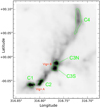 |
Fig. B.5 Apertures used to measure the parameters of the clumps discussed in the text. These apertures follow the level at the N(H2) peaks’ half intensity. They are superimposed on the N(H2) map. |
The dust distribution of the G316.80–00.05 field has been studied by Vig et al. (2007), based on observations obtained at 150 μm and 250 μm using the TIFR 100 cm balloon-borne telescope with a resolution of ~1′. Based on these observations, they consider this source to be mainly composed of two clouds, A and B, according to their nomenclature. Figure B.6 allows us to compare their observations with the Hi-GAL maps at similar wavelengths. Clumps C1 and C2 correspond to cloud A in Vig et al. (2007), while clumps C3N and C3S correspond to cloud B. The higher angular resolution of the Hi-GAL observations shows that the A and B clouds are not homogeneous but are composed of several structures. Clouds A and B were modelled by Vig et al. as spherically symmetric clouds of dust and gas. According to these authors, thegas exists throughout the clouds. Each cloud is ionised by a massive star located in the central zone that is devoid of dust. This zone is surrounded by a dusty shell. Our observations suggest: i) clouds A and B are not spherical structures, but are composed of several individual structures, as shown by Fig. B.6, ii) they are not ionised in their centre; this is especially evident for cloud B, as the radio-continuum and the 24 μm emission do not come from its central zone.
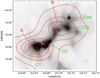 |
Fig. B.6 Comparison of the dust emission obtained at 160 μm by Hi-GAL (grey map; angular resolution ~12.5′′) and at 150 μm (red contours) by Vig et al. (2007, resolution ~1′, their Fig. 1) |
Observations of atomic or molecular lines have been obtained in the direction of the radio-continuum peak; their resolution is such that the brightest parts of the C1 and C2 clumps are covered by these observations (see Fig. B.2). The velocities measured are similar to that of the central H II region: V (CI) = − 38.8 km s−1 (Huang et al. 1999, beam ~ 130′′), V (CS) = − 37.8 km s−1 (Gardner & Whiteoak 1978, beam ~ 1.5′), V (CO) = − 39.3 km s−1 (Whiteoak et al. 1982, beam ~ 2.8′), V (NH3) = − 39 km s−1 (Vilas et al. 2000, beam ~ 4.2′); V (13CO) = − 38.9 km s−1 is also obtained in the direction of the bright rim bordering the C1 clump (Busfield et al. 2006, beam ~ 35′′). These measurements show that clumps C1 and C2 are associated with the central bipolar nebula.
Clump C4 lies farther from the H II region (e.g. see Fig. B.4a); the dense gas (i.e. CS emission) velocity in the direction of C4 is − 38.5 km s−1 (Jackson et al. 2008), meaning that it is also most probably associated with the H II region.
Three spots of OH, H2O, and methanol maser emission are detected in the direction of clumps. Their coordinates and velocities are given in Table B.2. Clump C1 harbours one of these maser sites (position accuracy of OH maser is better than 0.4′′; Caswell 1998); it lies on theborder of C1, behind the bright rim bordering C1 (see Fig. B.7a). The velocity of the various maser emission is in the range –47 km s−1 to –37 km s−1; thus not very different from that of the central H II region. This confirms the association of the C1 clump with the central H II region. Longmore et al. (2007) have obtained interferometric observations in NH3 transitions and 24 GHz radio-continuum emission at high resolution ( ~10′′) of the central region (mainly in the direction of C1 clump). NH3 is a good tracer of dense molecular gas (critical density ~2 × 104 cm−3). The integrated intensity of the NH3 (1, 1) transition is presented in Fig. B.7a. It shows two cores: one of them coincides with the central zone of clump C1, the other one is observed in the direction of the OH maser. This agrees well with the high mean density estimated for the central zone of the C1 clump (density ~ 7 × 105 cm−3; Table B.1). According to Longmore et al., the second core is probably an envelope surrounding the maser source. Two cores are also observed in the radio-continuum at 24 GHz (Fig B.7b). They are observed in the direction of the SUMSS peak emission at 843 MHz7. The observations of Longmore et al. show that one of the radio cores lies in the direction of the maser; its size is 13′′ × 11′′, its flux 1.13 Jy (the corresponding ionising flux is that of an early B star; Smith et al. 2002). Their interpretation is that the young object forming there is massive enough to ionise the surrounding gas. The second peak lies in the direction of a zone of 8.0 μm emission as shown by Fig. B.7b.
Maser sources in the vicinity of G316.80–00.05.
The second OH, H2O, and CH3OH maser spot is located at l = 316. °7624, b = –00. °0115 (again the OH maser positional accuracy is better than 0.4′′; Caswell 2001), which corresponds to the location of the C3N clump; clump C3 is therefore probably associated with the nebula.
The third OH, H2O, and CH3OH maser spot lies in the direction of a small clump that seems to be adjacent to a 8.0 μm filament bordering the southern lobe; it lies behind the filament with respect to the ionised region. However, its velocity, in the range –28 km s−1 to –15 km s−1, is rather different from that of the H II region. Therefore, this star formation site is probably not associated with the bipolar nebula.
B.3 Infrared dark clouds
Numerous IRDC fragments are listed by Peretto & Fuller (2009) in the direction of G316.80–00.05, shown in Fig. B.8. As can be seen from Fig. B.8, the massive clumps C2, C3S, and C3N, are not identified as IRDC fragments by Peretto & Fuller (2009). Among the IRDC fragments, two (G316.786–0.044 and G316.821–0.062) lie along the central parental filament, one (G316.825+0.013) lies in the direction of a small isolated clump of column density 2.6 × 1022 cm−2, and a few other fragments are located between 8.0 μm filaments; their nature is uncertain as they do not correspond to individual structures in the column density map (the resolution of the column density map can, however, smooth out small structures detected in absorption at 8 μm). A few IRDCs located at the centres of the S110 and S111 bubbles are not real, dense structures.
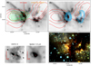 |
Fig. B.7 Vicinity of the first site of maser emission and the central region of the complex. The OH maser position isindicated by a red plus symbol. The orange arrow indicates the best candidate exciting star proposed by Vig et al. (2007). The red contours indicate the column density (levels of 1.0, 1.5, and 2.0 × 1023 cm−2). Panel a: green contours indicate the NH3 emission (Longmore et al. 2007, their Fig. 11); the underlying grey image is the Spitzer 8.0 μm image. Panel b: blue contours now indicate the radio-continuum emission at 24 GHz (Longmore et al. 2007). Panel c: composite JHKs colour image (VISTA images) showing the dark absorption features and the exciting star proposed by Vig et al. (2007). A zoomed view of maser site at 2.2 μm (VISTA) and 4.5 μm (Spitzer) is shown in the bottom-left panel. |
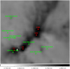 |
Fig. B.8 Positions (green crosses) of the IRDC fragments in the central area of G316.80–00.05. The underlying grey image is the column density map. The clump locations are shown in red crosses. |
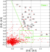 |
Fig. B.9 Colour–colour diagram, [3.6]–[4.5] vs. [5.8]–[8.0], for all Spitzer-GLIMPSE sources with measurements in the four bands, and situated within 10′ from the radio peak of the G316.80–00.05 field. The location of YSOs dominated by a disk (Class II YSOs) and by an envelope(Class I YSOs) are indicated, following Allen et al. (2004; see also Megeath et al. 2004). The sources discussed in the text, mainly candidate Class I YSOs, are identified. |
B.4 Young stellar objects and star formation
According to the GLIMPSE colour–colour diagram, several candidate Class I YSOs lie in the vicinity of the bipolar nebula; they are identified in Fig. B.9. Most of these sources are detected at 24 μm, which allows us to determine their evolutionary stages. Their coordinates, photometric magnitudes, and [8]–[24] colours are given in Table B.4.
Small regions of extended emission present in the field of G316.80–00.05.
Young stellar objects in the vicinity of G316.80–00.05. The JHKs magnitudes are from the VISTA catalogue.
First, we discuss the YSOs at the locations of the maser emission, then other YSOs in the field. Fig. B.7 shows the location of the first maser emission. As can be seen, a bright 70 μm compact source lies ~1.6′′ from the first maser position. Its flux of 1550 ± 100 Jy corresponds to a luminosity about 26000 ± 2000 L⊙. Its luminosity and the radio flux (see Appendix B.2) suggest that it is a compact H II region ionised by an early B star. This source would be young enough to be still associated with maser emission. The proximity ofa bright rim very close to the maser may suggest that at least a fraction of the radio-continuum and 70 μm emission comes from a dense ionised layer adjacent to the ionisation front and from the adjacent warm PDR, respectively. The VISTA K image (Fig. B.7c) shows an elongated feature on each side of the maser source, suggesting the presence of a jet. Also, a bright 4.5 μm source lies in the direction of the maser; it presents an extension (along the jet direction) suggesting that we are possibly dealing with an outflow such as EGO. A bright 8.0 μm source lies in the same direction; at 24 μm, the region issaturated. We have there an exceptional case of a MYSO young enough to present an outflow and massive enough to ionise its surrounding medium. This region is also especially interesting in terms of star formation as the MYSO is located not in the very centre of a dense clump but on its border, very close to the IF. There, we observe massive-star formation in a layer adjacent to the ionised gas (possibly a layer compressed by the ionised gas) and not at the very centre of the clump.
At the location of the second maser position lies a Class I YSO, our source #4 (Fig. B.10). This YSO is a very bright 24 μm (saturated) and 70 μm source. Its 70 μm flux of 227 Jy indicates a luminosity ~3700 L⊙. This source lies in the direction of the C3N clump, at about 9′′ from the column density peak. Several other YSOs also lie in the vicinity of the C3 clump. Sources #3 and #6 are Class I YSOs (based on their [8]–[24] colours). YSO #6 is not detectable at 70 μm (flux ≤ 0.3 Jy according to the CuTEX catalogue, which corresponds to a luminosity ≤7 L⊙). YSO #3 has a nearby companion (in projection) which is probably a Class II. YSO #3 has a 70 μm counterpart, of flux ~3.4 Jy, indicating a luminosity ~70 L⊙. YSO #7 is possibly a low-luminosity flat-spectrum source. YSOs #2 and #5 have faint 24 μm counterparts but are located too close to the maser source to be measurable; for the same reason, they are not detectable at 70 μm. Source #1 is located in the direction of the bright filaments bordering clump C3S; its 8.0 μm magnitude is probably influenced by the nebulous 8.0 μm background emission (its evolutionary stage is therefore very uncertain).
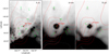 |
Fig. B.10 Vicinity of the C3 clump and the second site of maser emission. The YSOs and diffuse emission regions (A, B, and C) discussed in the text are identified. The red contours are for the column density (levels of 0.5, 1.0, 1.5, and 2 × 1023 cm−2). |
YSO #11 is observed in the direction of the third maser spot; its GLIMPSE colour points to a Class I YSO; the 4.5 μm image showsthat it is probably an EGO. The nearby source #10 is also a Class I according to its GLIMPSE colour. At 24 μm, sources #11 and #10 are not separated and the composite source is saturated. A bright 70 μm compact source lies in their direction. Several other YSOs lie nearby (see Fig. B.11). Sources #8 and #9 are observed in directions where the column density is ~6 × 1022 cm−2. Considering their GLIMPSE colours, they appear as Class I YSOs; considering their [8]–[24] colours (respectively 5.44 and 3.52 for #8 and #9), source #8 is confirmed Class I and source #9 is possibly a flat spectrum YSO. Source #8 is detected at 70 μm.
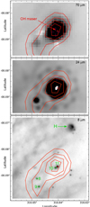 |
Fig. B.11 Third site of maser emission at 8 μm, 24 μm, and 70 μm. The OH maser position is indicated with a red arrow. The red contours are for the column density (levels of 4, 5, 6, and 7 × 1022 cm−2). The diffuse extended region, H, is identified in the 8 μm image. |
Many sources are observed along the parental filament, outside of the ionised region, especially in the direction of the C4 clump (Fig. B.12). Several of these sources have been discussed by Ragan et al. (2012). According to their [8]–[24] colours, sources #2 and #31 are Class I, sources #12, #18, #19, #20, #22, and #28 are flat spectrum YSOs, sources #13, #14, #15, #25 are Class II YSOs, and source #26 is of uncertain nature. Several of these Class II sources lie in directions of high column density (higher than 7.5 × 1022 cm−2, corresponding to AV ≥ 80 mag); if they are located behind such material their high extinction could explain their position in the GLIMPSE colour–colour diagram (the [3.6]–[4.5] colour is increased by ~1.1 mag for AV ~ 80 mag according to Indebetouw et al. (2005); furthermore the GLIMPSE and MIPSGAL photometry of source #15, the most extreme case, is of low accuracy; this YSO could be a flat-spectrum source as its [8]–[24] colour is 3.06 ± 0.29). The very bright source #17 is probably an unrelated evolved star, as its WISE colours indicate that it is an OH/IR star rather than a Class I/II YSO.
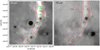 |
Fig. B.12 Sources in the vicinity of the C4 clump and along the parental filament. The red contours are for the column density (levels of 0.5, 0.75, 1.0 × 1023 cm−2). The diffuse extended region, F, is also identified. |
Several other sources lying in the vicinity of C4 are only 24 μm and/or 70 μm sources8. As such, they are possibly younger than Class I YSOs, possibly Class 0 YSOs or even prestellar sources if only detected at 70 μm. Sources #23, #24, #29, and #30 are observedonly at 70 μm. The faint sources #16 and #27 observed at 24 μm are of uncertain nature.
A few other sources lie farther away from the central parts of the bipolar nebula and the parental filament. Their association with the bipolar nebula is more uncertain. They are the YSOs #32, #33, #34, #35, #36, #37, #38, and #39, identified in Fig. B.13. YSO #32 lies in the direction of the northern lobe (inside it); it is probably a Class II YSO. YSO #33, located in the direction of the north-west border of the north lobe (inside it), is probably a Class I YSO (it has no detectable 70 μm counterpart). YSO #35 has no clear detectable 24 μm counterpart and YSO #36 lies in the 24 μm saturated zone; their nature is uncertain. The same situation holds for YSO #34 lying inside S110 (column density ~2.1 × 1022 cm−2), in the saturated 24 μm zone. YSO #37 is observed in the direction of a small clump with a column density ~7.4 × 1022 cm−2. This clump also contains the two small diffuse regions E and G (discussed in Appendix B.5). The clump lies along a 8.0 μm filament on the west side of the S111 bubble. YSO #37 is probably a Class II YSO according to its [8]–[24] colour. Along the same filament lies another small clump, with a column density of ~5.0 × 1022 cm−2, which contains the Class I YSO #38 (YSO #38 has no detectable 70 μm counterpart). YSO #39 lies in the direction of a small clump of column density ~3 × 1022 cm−2, located on the south border of S111; its 70 μm flux indicates a luminosity of 140L⊙ if at the distance of 2.8 kpc and it is probably a flat-spectrum YSO.
B.5 Small regions of extended diffuse IR emission
Eight small regions of extended diffuse emission at 8 μm, 24 μm, and 70 μm lie in the field of G316.80–00.05. They are the regions A, B, C, D, E, F, G and H identified in Fig. B.13. Theircoordinates and photometric measurements are given in Table B.3. Region A is located along the parental filament in the C3 clump, while B and C are located on the eastern border of the C3 clump (see Fig. B.10 for enlarged view). Region D lies below the parental filament close to clump C3 (see Fig. B.14 for enlarged view). Region F lies on the western border of C4 (see Fig. B.12 for enlarged view). Regions E and G are located at the south-western side of clump C3 and region H lies close to the third maser site (see Fig. B.11 for enlarged view). The column density in the direction of these regions is always higher than 2.5 × 1022 cm−2. We do not know if these regions are associated with the bipolar nebula.
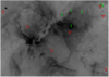 |
Fig. B.13 Locations of diffuse extended regions in the field of G316.80–00.05. The underlying grey image is the 8 μm image. |
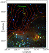 |
Fig. B.14 JHKs colour composite image, showing the second site of maser emission (green cross) and the extended region D (surrounded by a green dashed line). The red contours are for the column density (same levels as in Fig. B.7). The proposed exciting star of the region D is indicated by an arrow. |
A star lies at the very centre of region C; if region C lies at 2.8 kpc, then the 2MASS photometry of the star suggests that it is a B1V star with a visual extinction of 33.1 mag. This star is probably the main heating source of the dust in this region, and region C is possibly a faint H II region.
Region D appears as a small cometary nebula on the Spitzer-IRAC images. A star lies at its centre, visible in the VISTA K-band and Spitzer 4.5 μm images (see Fig. B.14). Only faint emission is observed at SPIRE wavelengths. The highest dust temperature in the field is observed in the direction of this region (see discussion in Appendix B.2); this suggests that we are possibly dealing with a compact H II region. We do not have high-resolution radio-continuum emission that could confirm this classification. However, the SUMSS radio-continuum emission extends in this direction (see Fig. B.2), indicating unresolved radio continuum emission. If it is associated (and therefore at the same distance), the central star is possibly an O9V star with a visual extinction of 33.2 mag. This is a strong argument in favour of this region being a compact H II region.
Appendix C G320.25+00.44
As shown in Fig. C.1, G320.25+00.44 is a bipolar nebula. It has two lobes of different size (the north-eastern one is about three times larger than the south-western one). A filament crosses its waist. The filament is seen in absorption in the near- to mid-IR (up to 24 μm), and in emission at Herschel-SPIRE FIR wavelengths. Extended 24 μm emission is observed from the central region.
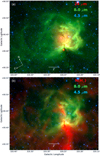 |
Fig. C.1 Bipolar nebula G320.25+00.44. Panel a: composite colour image, with red, green, and blue indicating the 24 μm, 8.0 μm, and 4.5 μm emissions, respectively. The lobes, the central extended 24 μm emission, and a few compact 24 μm sources at the waist of the nebula are apparent in this image. Panel b: composite colour image, with blue, green, and red showing the 4.5 μm, 8 μm and column density maps, respectively. |
Hα emission is present in the direction of the two lobes, and is strongly absorbed along the filament at the waist (Fig. C.2). This nebula is also a radio source at 843 MHz (from SUMSS survey). The peak of radio emission coincides with the region of extended 24 μm. However, the absence of Hα emission corresponding to the zone of strong 843 MHz emission points to the presence of high extinction towards the central area of the nebula.
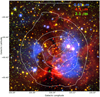 |
Fig. C.2 Central region of G320.25 + 00.44 at optical and NIR bands. Red indicates the 4.5 μm emission (shows the presence of a small cluster at the very centre of the nebula) and green shows the Ks VISTA image. The Hα SuperCOSMOS image is shown in blue. The white contours correspond to the radio emission at 843 MHz for the central region (contour levels of 0.015, 0.09, 0.16, and 0.23 Jy beam−1). The green cross corresponds to the position of IRAS 15033–5736. |
This H II region is also known as RCW88 (Rodgers et al. 1960). In the past it was identified as a planetary nebula (PN 166 in the list ofWray et al. (1966), but more recently it was recognised as being a “misclassified planetary nebula” and more probably a diffuse H II region (Acker et al. 1987).
C.1 Exciting star and distance
The velocity of the H II region is V (Hα) = −32.3 km s−1 according to Georgelin et al. (1987) or V (H109α) = −31 km s−1 according to Caswell & Haynes (1987). These authors favour a near kinematic distance in the range 2.1–2.2 kpc, which we adopt in this work. Avedisova & Kondratenko (1984) estimate the distance to be 1.8 ± 0.2 kpc, from the photometry of two faint OB stars; however these stars lie more than 18′ from the nebula and therefore are not directly associated with it. We note that the presence of observable Hα emission favours a near kinematic distance.
The integrated flux density of the H II region is S(5 GHz) = 2.3 Jy (Caswell & Haynes 1987); this agrees with the peak flux density of 2.06 Jy at 4.85 GHz measured by Kuchar & Clark (1997). Assuming a distance of 2.1 kpc, an electron temperature of 8000 K, the integrated flux at 5 GHz points to an ionising photon flux of 9.6 × 1047 s−1, and therefore to an exciting star of spectral type O8.5–O9V.
As shown by Fig. C.2, a small cluster is present in the central region of the nebula, as an over-density of sources at 4.5 μm. According to Mercer et al. (2005) this cluster (coordinates: l = 320. °245, b = +00. °436) contains 113 stars in a circular aperture of radius 1′; it lies close to the centre of the radio source (also the centre of the extended region of 24 μm emission). We have used the VISTA catalogue to identify the exciting star(s). Figure C.3 shows the J vs. J − K diagram of all the stars (small red circles) located at less than 10′ from the centre of the radio-continuum emission. The main sequence has been drawn for the assumed distance of 2.1 kpc. We searched exciting star(s) of the nebula within 0.5 pc (0.82′) radius from the radio centre (coordinates: l = 320. °244, b = +00. °439); these sources are marked with blue symbols in the Fig. C.3.
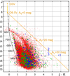 |
Fig. C.3 J vs. J − K diagram for the stars located at less than 10′ from the centre of the radio-continuum emission (red symbols). The main sequence for O stars (Martins & Plez 2006) and low-mass stars (Pecaut & Mamajek 2013) are drawn in orange and black curved lines, respectively, for a distance of 2.1 kpc and zeroreddening. The reddening vector corresponding to an O9.5 star is drawn as a slanting line using the extinction law of Rieke & Lebofsky (1985). The green and blue symbols represent stars located at less than 1 pc and 0.5 pc from the 24 μm centre, respectively. Possible exciting stars are numbered as #1, #2, and #3 in the figure. They are identified in Fig. C.4. |
In Fig. C.3, the three probable candidate exciting stars are labelled as #1, #2 and #3. These stars are the likely O stars in the direction of the peak radio emission. We give their coordinates and photometricmeasurements in Table C.1. Figure C.4 shows their locations on the JHKs colour-composite image. Among the stars, star #1 lies the closest to the radio and 24 μm centre, and thus is our best candidate exciting star. It is affected by a visual extinction of the order of 35.0 mag. Star #1 is the most massive star, too massive for a distance of 2.1 kpc. It is worth noting that star #1 has a nearby red companion that is not present in the VISTA catalogue, but can be seen in the VISTA image; therefore the K magnitude of star #1 is possibly overestimated. Star #2 lies farther away from the radio centre. Its photometry agrees with an O9V star at a distance of 2.1 kpc, with a visual extinction of 28.2 mag. Star #3 lies even farther away from the radio centre; its photometry suggests for an early B star.
Likely exciting stars of G320.25+00.44. Data extracted from the VISTA catalogue.
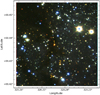 |
Fig. C.4 Central region of G320.25+00.44 in VISTA JHKS bands. The J-, H-, and Ks-band images are shown in blue, green, and red colours, respectively. The three candidate exciting stars are identified as #1, #2, and #3. |
Among the exciting stars, as can be seen from Fig. C.4, star #1 lies in the direction of the central parental filament. The cold material of the filament appears to be strong enough to absorb the 24 μm emission, the reason being that one sees two peaks of 24 μm emission on each side of the filament (Fig. C.1a). We suggest that the filament is responsible for the strong absorption of star #1 ( ~35 mag). Star #1 liesat the centre of the group of stars prominent in the GLIMPSE images or cluster identified by Mercer et al. (2005), and is therefore likely the exciting star of the nebula, although we cannot completely ignore the possibility that star#2 fulfills this function. Among the stars of the cluster with H and K magnitudes, we estimate a visual extinction of up to 41 mag, assuming an intrinsic colour H − K ~ 0 mag for the starsand using the extinction laws of Rieke & Lebofsky (1985). The column density measured in this direction is 2.8 × 1022 cm−2, which corresponds to an extinction of ~30 mag. This discrepancy points to an underestimate of the column density, and thus tells us that the absorbing structures are smaller than the resolution of our column density map ( ~18′′).
C.2 Dust temperature, column density, and molecular clumps
Figure C.5 shows the dust temperature map of G320.25+00.44. As can be seen, the parental filament outside the H II region is cold, with a temperature in the range of 1.7 to 17K. Among the lobes, the western lobe is relatively warmer with a temperature higher than 21 K and a maximum of 23.8 K. The western lobe is also bright at 8 μm. The extended eastern lobe is colder but, as a whole, has a temperature higher than 19 K.
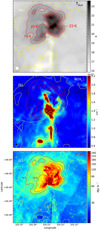 |
Fig. C.5 Dust temperature map in the field of G320.25+00.44. The red contours are for temperatures of 19 K, 20 K, 21 K, 22 K, and 23 K. The yellow contours are for temperatures of 16 K, 17 K, and 18 K. They are superimposed on the temperature map (panel a), the column density map (panel b) and on the 8.0 μm image (panel c). |
Figure C.6 shows the column density map of G320.25+00.44 along with the locations of bright clumps (marked as C1, C2, and C3) observed in its direction. The parameters of these clumps are given in Table C.2. As can be seen from the figure, the parental filament has a column density in the range 2 × 1022 cm−2 to 4 × 1022 cm−2. Among the clumps, the C1 clump is massive (mass ~ 280 M⊙), compact (radius ~ 0.12 pc), and dense (density ~ 5.7 × 105 cm−3). It is present at the waist of the bipolar nebula, adjacent to the ionised region. C2 lies outside of the parental filament, and is less massive (mass ~ 120 M⊙), less compact(radius ~ 0.21 pc), and less dense (density ~ 4.1 × 104 cm−3) than C1. It is, however, the coldest structure of the field, and four candidate Class I YSOs are detected in its direction (discussed in Sect. C.4). Its velocity, V (CS) = –32.1 km s−1 (Jackson et al. 2008), which is similar to that of the ionised gas, indicates that the C2 clump lies at the same distance as G320.25 + 00.44. The clump C3 is highly elongated and less dense among the clumps.
Properties of the clumps in the field of G320.25+00.44.
From Fig. C.6 one can also see that a relatively high-column-density structure (indicated with arrows) surrounds the western lobe. We suggest that it was formed from material collected during the expansion of the ionised gas as observed in the case of several Galactic H II regions (e.g. Deharveng et al. 2010). The column density of this structure is in the range 1.1 × 1022 cm−2 to 1.7 × 1022 cm−2.
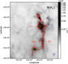 |
Fig. C.6 Column density in the field of G320.25+00.44. The contours correspond to column density levels of 0.15, 0.2, 0.5, and 1.0 × 1023 cm−2. The clumps are identified as C1, C2, and C3. The blue arrows show the matter likely collected around the western lobe of the nebula during its expansion. |
C.3 Infrared dark clouds
Several dark clouds have been detected in the direction of this region. For example, using J-band absorption, Hartley et al. (1986) have detected a cloud, DC320.2+0.4 (exact coordinates given by Dutra & Bica (2002): l = 320. °247, b = +0. °422) in the field of G320.25+00.44. This cloud corresponds to the border of the clump C1. We know that this clump is associated with the nebula because its velocity is similar to that of the ionised gas, with V (CO) = –32.9 km s−1 (Otrupek et al. 2000). Likewise, using an NIR extinction map, Dobashi (2011) detected a dark cloud (their number 6235) in the direction of l = 320. °233 and b = +0. °400. This cloud also lies at the border of the bright C1 clump (see Fig. C.7).
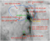 |
Fig. C.7 IRDCs in the field of G320.25+00.44. The IRDCs identified by Peretto & Fuller (2009) are in red, the ones identified by Hartley et al. (1986) and Dobashi (2011) are respectively in green and yellow. The underlying grey image is the column density map; the green contours correspond to column densities of 1.5 × 10²², 2.5 × 10²², and 10 × 1022 cm−2. The blue contour indicates the extent of the bipolar nebula. |
Several other IRDC fragments have also been identified in the direction of G320.25+00.44 by Peretto & Fuller (2009). The locations of these fragments are shown in Fig. C.7 with red plus symbols. Several of them correspond to real structures. They are SDC G320.262+0.467, SDC G320.252+0.447, SDC G320.235+0.346, SDC G320.234+0.331, SDC G320.271+0.293, and SDC G320.284+0.287. Four are likely false detections: i) SDC G320.219+0.430, which corresponds to a low brightness region of the western lobe; ii) SDC G320.322+0.469 and SDC G320.291+0.408 inside the eastern lobe; and iii) SDC G320.281+0.501, which corresponds to a low-brightness region close to periphery ofthe western lobe. We note that the most massive clump, C1, which is a strong absorption feature at 8.0 μm, has not been identified as an IRDC fragment by Peretto & Fuller (2009).
C.4 Young stellar objects and star formation
Figure C.8 shows the [3.6]–[4.5] vs. [5.8]–[8.0] diagram for the point sources in the field of G320.25+00.44. All the YSOs discussed in the text are identified in Fig. C.9. Their coordinates and photometric measurements are given in Table C.3. As can be seen from Fig. C.9, several of these YSOs are located outside the two lobes, and therefore are probably not associated with the bipolar nebula. They are the sources #7 and #19 (located far from the lobes), and #1 and #2 (located in the direction of filaments bordering the left lobe). We note that the [5.8]–[8.0] colour of YSOs #8and #12 (located in the central regions of the bipolar nebula) is suspicious as their emissions at 8 μm are extended and faint.
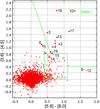 |
Fig. C.8 Colour–colour [3.6]–[4.5] vs. [5.6]–[8.0] diagram of the GLIMPSE sources in the vicinity of G320.25+00.44. These sources lie less than 9′ from the exciting cluster and have measurements in the four bands. The sources discussed in the text, mainly candidate Class I YSOs, are identified. |
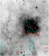 |
Fig. C.9 Positions of the various sources discussed in the text in the field of G320.25+00.44. The underlying grey image (in logarithmic units) is the 24 μm image. The blue contours are for the column density (levels of 1.5 × 1022 cm−2 and 5 × 1022 cm−2). |
Sources in the field of G320.25+00.44 (sources discussed in the text).
Many sources are present in the MIPSGAL image at 24 μm, but most of these sources populate the zone around 0,0 in the GLIMPSE colour–colour diagram. They are therefore not Class I sources. Looking at the [8.0]–[24] colour of the IRAC YSOs, we confirm that YSOs #3, #4, #10, #13, #16, #17, and #18 are likely Class I sources; YSOs #1, #2, and #14 are flat-spectrum sources; and YSO #19 is probably a Class II source.
The Herschel-70 μm image shows very few sources around the bipolar nebula, with only a bright 70 μm source observed in the direction of the C1 clump (see Fig. C.10). The 70 μm peak agrees well with the peak of the column density. The 70 μm source is slightly extended, with an integrated flux at 70 μm of 90 ± 10 Jy, which points to a total luminosity of ~1000 L⊙. At 24 μm this source has three components: YSOs #9 and #11 of similar brightness, and a fainter component #10 (Fig. C.10). At 8.0 μm, source #9 appears faint and extended, and source #11 is not seen, likely due to the fact that it is locatedin the direction of a strong absorption feature that seems to divide the extended 8.0 μm emission region in two.
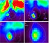 |
Fig. C.10 Spatial location of candidate YSOs in the direction of the C1 clump. The blue contours correspond to column densities of 0.5 × 1023 cm−2 and 1 × 1023 cm−2; they represent the emission in the central direction of the C1 clump and are superimposed on the 8.0 μm (panel a), 24 μm (panel b), 70 μm (panel c), and column density (panel d) maps. The YSOs are identified by plus symbolss. |
The 70 μm source is slightly elongated, as is the #9+#11 source, but the peak of the 70 μm emission does not correspond to either the #9 or the #11 YSOs; there is a positional discrepancy of some 3–4′′. The positional accuracy of the Herschel images is of the order of a few arcseconds, especially for regions located on the border of the maps, which is the case for G320.25+00.44. We therefore suggest that the 70 μm source corresponds to YSOs #9+#11. However, due to the lack of resolution, we do not know if we are dealing with two point-sources or with a single slightly extended source.
In the direction of C1, around Class I YSO #16, we also observed faint 70 μm emission (4.3 Jy, CuTEX).
To conclude, the Class I YSOs are all observed in the direction of high-column-density clumps or features; Class I YSOs #3 and #4 are observed in the direction of C2. The C1 clump contains at its very centre the high-luminosity source formed by YSOs #9+#10+#11 and its 70 μm counterpart. Class I YSOs #13, #16, and #17 are observed on the border of C1, and Class I YSOs #14 and #18 close to C1, along the parental filament.
Figure C.11 shows the unsharp masked image of the nebula at 24 and 70 μm along with the distribution of Class I YSOs and dense gas in its vicinity. The massive clump C1 lies at the western side of the nebula (adjacent to the H II region), and the most luminous YSO of the field is embedded in C1 and lies close to a bright rim (clearly visible as a convex feature in the 70 μm image with its apex pointing towards the exciting star of the nebula) bordering the clump. Other Class I YSOs in the vicinity of C1 are located far away from the clump centre. We do not see strong dust peaks around these Class I YSOs, which could be due to the low-luminosity nature of these YSOs (they have no 70 μm counterparts). It is difficult to conclude a great deal about the origin of the Class I YSOs that are located far away from the H II region, but since the clump C1 is adjacent to the H II region and shows a bright rim feature, we suggest the formation of the clump (and therefore the YSOs embedded in the clump) is strongly influenced by the compression of the H II region.
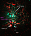 |
Fig. C.11 Colour composite image showing the position of the various sources that are discussed in the text, with respect to the 24 μm emission (in turquoise), the 70 μm emission (in red), and the column density distribution (contours). |
Appendix D G338.93–00.06
G338.93–00.06 is a rather faint bipolar nebula. The two lobes are clearly visible in 8 μm data, as shown by Fig. D.1a. The parental filament is not extended. At the waist of thenebula, the molecular material forms an elliptic structure, seen in absorption at 8.0 μm and in emission at SPIRE wavelengths (Fig. D.1b). Extended 24 μm emission is present in the centre of the nebula.
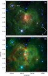 |
Fig. D.1 Composite colour images of G338.93–00.06. In the above images green and blue colours show the Spitzer 8.0 μm and 4.5 μm emissions, respectively. Panel a: the Spitzer 24 μm emission (saturated in the central region) is shown in red. Panel b: the Hi-GAL 250 μm emission of the cold dust is shown in red. |
The SuperCOSMOS image shows Hα emission near the waist of the nebula (see Fig. D.2a), mainly inside the elliptical structure. We note that faint diffuse Hα emission has also been observed in the direction of G338.93–00.06. This diffuse emission is probably due to unrelated ionised material present along the line of sight, as Georgelin et al. (1996) have shown the presence of several ionised features at different velocities (and therefore different distances) along the line of sight. This nebula is a radio-continuum source (Caswell & Haynes 1987).
A small cluster is reported by Dutra et al. (2003) near the centre of the elliptical structure (coordinates: l = 338. °931, b = –00. °065). This region is also the location of an IRAS source, IRAS 16395–4600 (coordinates: l = 338. °9279, b = –00. °0551). Figure D.2a shows the radio and optical emission in the central area of the nebula, along with the locations of the IRAS source and the embedded sources of the cluster.
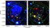 |
Fig. D.2 Central region of G338.93–00.06 at optical and NIR bands. Panel a: colour composite image with red, green, and blue showingthe Ks-band, J-band, and Hα emissions, respectively. Panel b: the red, green, and blue colours now show the Spitzer 4.5 μm, Ks, and J emissions, respectively. The green contours are for the radio emission (SUMSS survey; levels of 0.3, 0.4, and 0.5 Jy beam−1). The red cross corresponds to the position of IRAS 16395–4600, while the yellow cross corresponds to the coordinates of the stellar cluster reported by Dutra et al. (2003). Sources that are discussed in the text are labelled with numbers. |
D.1 Distanceof the region and exciting cluster
The velocity of the H II region measured through radio recombination line is V (H109α) = − 40 km s−1 (Caswell & Haynes 1987), which is in agreement with the velocity V (Hα) = –41 km s−1 of the Hα line (Georgelin et al. 1996). The kinematic distance of the region is uncertain to some extent. For example, Caswell et al. favour a near kinematic distance of 3.6 kpc. Based on the velocity ( − 38 km s−1) of the HI absorption line, Kothes & Dougherty (2008) estimated the distance of the H II region as 2.8 kpc. Georgelin et al. and Lee et al. (2012) favour a near kinematic distance of 3.1 kpc.
The integrated flux density of the H II region at 5 GHz as measured by Caswell & Haynes (1987) and Wilson et al. (1970b) is in the range 3.3–3.4 Jy. Kuchar & Clark (1997) measured a peak flux density of 3.925 Jy at ~5 GHz. If we adopt a distance of 3.1 kpc, an electron temperature of 6000 K (Caswell & Haynes 1987), and flux at 5 GHz in the range 3.3 Jy–3.9 Jy, we estimate the ionising photon flux to be in the range 3.34 × 1048–3.95 × 1048 s−1. We therefore propose a spectral type for the exciting star of O7V–O7.5V (if single and if no ionising photons are absorbed by dust internal to the region).
The exciting star of the nebula has not yet been identified. We searched exciting star(s) of the nebula close to the radio peak. As can be seen from Fig. D.2, an embedded cluster containing several NIR stars is associated with the nebula. To identify exciting star(s), we follow a similar prescription as employed for G320.25+00.44. In doing so, we found the star #1 of the Fig. D.2b is the best candidate O star according to its NIR photometry. Its JHKS magnitudes point to an O6V–O6.5V star if at 3.1 kpc or a O7V star, if at 2.8 kpc (visual extinction ~20 mag). Stars #2, #3, #4,#7, and #8 do not present a NIR excess, but they are not O stars; among them, star #7, if at 3.1 kpc, is possibly an early B star (visual extinction ~ 29 mag) and is therefore able to participate in the ionisation of the bipolar nebula. Stars #5 and #9 are possibly Class II YSOs according to their GLIMPSE colours (discussed in Appendix D.4). Star #10 is probably an evolved star, and star #11 appears to be a foreground star. In the following, we adopt the kinematic distance of 3.1 kpc.
D.2 Dust temperature, column density, and molecular clumps
The column density map of the field is presented in Fig. D.3 and the compact clumps are also marked. As can be seen, the dust present at the waist of the nebula lies mainly in four clumps. They are the clumps C1, C2, C3, and C4 of Fig. D.3. Among them, C1 and C2 are brighter than the others, with peak column densities of 2.5 × 1023 cm−2 and 1.6 × 1023 cm−2, respectively. We also see a clump on the border of the right lobe (clump C5 of Fig. D.3), and two clumps on the border of the left lobe (clumps C6 and C7 of Fig. D.3). The clumps C1 and C5 contain sources bright at 70 μm and associated with class II methanol masers, and are therefore sites of massive star formation. Among the clumps, C1 and C2, are compact and dense. The parameters of these clumps are given in Table D.1.
Properties of the condensations in the field of G338.93–00.06.
A remarkable feature of this nebula is its elliptical waist. This elliptical feature is seen at 8.0 μm, one half in absorption, the other half in emission; it is seen at PACS and SPIRE wavelengths in emission (see Fig. D.4). The four clumps, C1 to C4, are regularly spaced along this ellipse, two of them (C1 and C2) are massive (C1: 275 M⊙, C2:120M⊙) and dense ( ≥106 cm−3 for both).
For this nebula, material with column density in excess of 3.5 × 1022 cm−2 is observed surrounding the left lobe (see Fig. D.3). We suggest that we are dealing with material collected during the expansion of the lobe.
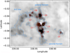 |
Fig. D.3 Column density map of the G338.93–00.06 field. The red contours are for the column density levels of 0.5, 1.0, 1.5, and 2 × 1023 cm−2, mainly showing the locations of the bright clumps. The blue contour corresponds to a column density level of 3.5 × 1022 cm−2. It mainly shows the collected material around the north-east lobe. The green contours are the aperture used to measure the mass and density for the central regions of the clumps. |
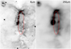 |
Fig. D.4 Elliptical waist of the G338.93–00.06 nebula at 8 μm and 250 μm. |
D.3 Infrared dark clouds
Seven IRDCfragments are reported by Peretto & Fuller (2009) in this region; they are identified in Fig. D.5a. Among the IRDCs: (i) four (SDC G338.928–0.086, SDC G338.928–0.112, SDC G338.930–0.079, and SDC G338.931–0.031) lie in the direction of small absorption features located along the parental structure, (ii) one (SDC G338.986–0.049) lies in the direction of the absorption feature located on the border of the left lobe, and (iii) two (SDC G338.962–0.058 and SDC G338.968–0.072) lie in the direction of the centre of the left lobe. All these IRDC fragments correspond to regions of cold dust emission. However, the two clumps, C1 and C5, with stronger emission at 250 μm, are not detected as IRDC fragments (see Fig. D.5b). These two clumps are associated with methanol masers, and are therefore sites of massive star formation.
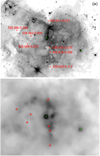 |
Fig. D.5 IRDCs reported in the field of G338.93–00.06 (red plus marks). Panel a: underlying grey image is the Spitzer 8.0 μm image. Panel b: underlying grey image is the Herschel 250 μm map. The positions of the methanol masers are shown by the green crosses. |
D.4 Young stellar objects and star formation
For G338.93–00.06 field, we do not present the [3.6]–[4.5] vs. [5.8]–[8.0] diagram as very few candidate YSOs are found in this field. The point sources identified as YSOs based on the GLIMPSE colours and/or association with methanol masers and/or detection at 70 μm are shown in Fig. D.6, and their coordinates and photometric measurements are given in Table D.2. We note that methanol masers are signposts of YSOs associated with outflows (Breen et al. 2010, and references therein).
Sources in the field of G338.93–00.06.
Two 6.7 GHz methanol masers are detected in the G338.93–00.06 field (Fig. D.6 for their locations). Their positions are given with asub-arcsecond accuracy by Caswell (1996, see Table D.2). One of them lies in the C1 clump. Its velocity is − 41.9 km s−1; therefore it is most probably associated with the bipolar H II region. The point source embedded in C1 is bright at 70 μm and 24 μm. This source is our YSO #2 (the maser lies at ~0.′′5 from YSO #2). Its WISE colours ([3.4] = 7.807, [4.6] = 5.663, [12] = 0.136, and [22] = –3.625 mag) have the characteristics of a Class I YSO according to Koenig et al. (2012) criteria. The second maser lies in the direction of the C5 clump; its velocity is − 41.4 km s−1, so very likely associated with the bipolar H II region. The corresponding point source is bright at 70 μm. This source is our YSO #4 (the maser lies at ~0.′′2 of YSO #4); its WISE colours ([3.4] = 7.224, [4.6] = 4.621, [12] = 2.029, and [22] = –0.263 mag) also have the characteristics of a Class I YSO. Both the masers show indications of variability9. The maser associated with YSO #4 is coincident with an OH 1665 & 1667 MHz maser (Caswell 1998); the OH maser positions have typical rms uncertainties of 0.4′′). No OH maser is detected in the direction of the methanol maser associated with YSO #2. YSO #2 has a 70 μm flux of 193 Jy indicating a luminosity of ~4500L⊙, if at 3.1 kpc. YSO #4 has a flux of 124 Jy, indicating a luminosity of ~2900L⊙. The luminosity and evolutionary status of the YSOs #1 and #2 suggest that massive star formation is currently taking place in clumps C1 and C2.
A few other sources (YSOs #1, #3, and #5) are also candidate Class I YSOs according to the [3.6]–[4.5] vs. [5.8]–[8.0] diagram. YSO #1 is located in the central region, along the elliptic feature at the waist of the bipolar nebula; it is bright at GLIMPSE wavelengths, but has no 24 μm or 70 μm counterpart.Therefore, its nature is uncertain; it is possibly a low-mass YSO. YSO #5 is located near the left lobe, slightly outside of it; its association with the nebula is uncertain. Its [8.0]–[24] colour suggests that it is a flat-spectrum source. YSO #3 is very faint at GLIMPSE wavelengths; it has no counterpart at longer wavelengths; its nature is uncertain.
The IRAS source, IRAS 16399–4601, is saturated at all Spitzer wavelengths up to 24 μm (Fig. D.6). Its WISE magnitudes are: [3.4] = 2.219, [4.6] = –0.258, [12] = –1.053, and [22] = –2.214. Its WISE colours suggest that it is not a Class I YSO, and probably not even a Class II (see Koenig et al.’s criteria); it is most probably a C-rich AGB star (e.g. see Tu & Wang 2013), and therefore an evolved star. Clump C5 harbouring YSO #4 is probably a pre-existing clump reached and compressed by the IF limiting the right lobe. Clump C1 harbouring YSO #2 lies at the waist of the bipolar nebula in the most massive clump of the field; it does not lie in its centre but at equal distance ( ~0.1 pc) in projection from the column density peak and the bright rim bordering C1 on its side turned towards the H II region. The formation of both MYSOs was probably triggered by the bipolar nebula, but via different processes.
Clump C2 is probably a protostellar clump. It appears in absorption at 8.0 μm and therefore probably lies on the front side of the waist. It contains no detectable IR source up to 24 μm and is unresolved on the column density map, and very dense. It is bordered by a bright rim at 8.0 μm on its side turned towards the ionised region. It contains a 70 μm source witha flux of 20.7 Jy indicating a luminosity of ~540L⊙.
D.5 Small extended emission regions
In the vicinity of the nebula (outside the lobes) lies a 24 μm compact bubble with a clumped morphology, surrounding a central point source (coordinates: l = 338. °9977, b = –00. °0082); it is identified as “MN46” in Fig. D.1a. According to Gvaramadze et al. (2010), MN46 is a candidate luminous blue variable and therefore an evolved massive star. The nature of this compact bubble is discussed by Nowak et al. (2014); its estimated distance is 1.9 kpc, and therefore it is probably not associated with the bipolar nebula.
Two compact regions are observed along the top border of the left lobe, between the C6 and C7 clumps. Their locations suggest that they are probably associated with the central nebula. They are identified in Figs. D.6 and D.7 as regions #1 and #2, and their coordinates and photometric measurements are given in Table D.3. Region #1 is an empty circular bubble at 8 μm, the more extended of the two regions, with a radius ~10′′, and is filled by 24 μm and 70 μm emission (see Fig. D.7). Region #2, which seems in projection to be adjacent to region #1, is more compact (radius ~ 5.′′ 5) and is also brighter at 24 μm and 70 μm.
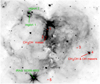 |
Fig. D.6 Location of the various sources discussed in the text in the field of G338.93–00.06 (the YSOs are in red). The underlying grey image is of Spitzer 8.0 μm data. |
Fluxes of small extended regions.
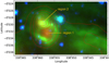 |
Fig. D.7 Two compact regions of extended 8.0 μm, 24 μm, and 70 μm emission lying on the border of G338.93–00.06. Red, green, and blue colours show the 24 μm, 8.0 μm, and 4.5 μm emissions, respectively. The red contours indicate the 70 μm emission (levels of 2000 MJy sr−1 to 8000 MJy sr−1 by s-eps-converted-to.pdf of 1000 MJy sr−1). |
Appendix E G339.58–00.12
G339.58–00.12 is a bipolar nebula presenting two closed lobes of unequal size (Fig. E.1). The parental filament is relatively faint at Herschel-SPIRE wavelengths. It is especially conspicuous on the Spitzer 8.0 μm image, where it appears as a clumpy absorption feature formed of multiple filaments.
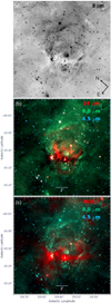 |
Fig. E.1 Bipolar nebula G339.58–00.12. Panel a: Spitzer 8.0 μm image showing the parental filament in absorption. Panel b: colour composite image with the Spitzer 4.5 μm, 8.0 μm, and 24 μm emissions shown in blue, green, and red, respectively. Panel c: red now shows the column density, showing the presence of two clumps along the parental filament. |
Figure E.2 shows the radio emission of the nebula at 843 MHz. As can be seen, the radio emission is especially bright at the waist of the nebula, and is also present along the lobes. One can also see the presence of two compact radio sources at the north-west of the bipolar nebula, the brightest one at l = 339. °522, b = –00. °026 and the other one atl = 339. °536, b = –00. °004. These compact sources are probably from background galaxies, since there is no IR emission in their directions.
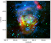 |
Fig. E.2 Radio-continuum emission of the bipolar nebula G339.58–00.12. The image is a colour composite, with 843 MHz radio-continuum emission (SUMSS) in red and Spitzer 24 μm and 8.0 μm emission in green and blue, respectively. The contours indicate radio emission levels of 0.025, 0.050, 0.075, 0.100, and 0.125 Jy beam−1. |
No Hα emission is detected in the direction of the H II region, even on the SuperCOSMOS image, which indicates a high level of extinction in its direction. No exciting cluster has been identified in the literature, probably the result of this high extinction.
E.1 Distanceand exciting cluster
Kothes & Dougherty (2007) estimated a distance of 2.6 kpc (+1.3 kpc, –0.7 kpc) for the region, based on the HI absorption line and adopting a systemic velocity of − 34 km s−1. The velocity of the ionised gas is at V (H109α) = − 30 km s−1, and the velocity of dense molecular gas detected with H2CO line in absorption is at V (H2CO) = − 33 km s−1 (Caswell & Haynes 1987).
According to Caswell & Haynes (1987), this H II region has an integrated flux density of 3.4 Jy at 5 GHz. At 4.85 GHz, Kuchar & Clark (1997) measured a peak flux density of 2.29 Jy. Assuming a distance of 2.8 kpc (discussed below), an integrated flux of 3.4 Jy at 5 GHz, and an electron temperature of 8000 K, we estimate the ionising photon flux NLyc to be ~2.53 × 1048 s−1, which points to an exciting star of spectral type O7.5V.
We expect the exciting star to be in the central area of the nebula. Just above the parental filament, we find that there is a diffuse region that is relatively bright at 8.0 μm with a nearby bright star (e.g. see 8 μm image of Fig. E.1a). The 8 μm Spitzer band contains the 7.7 and 8.0 μm emission lines, commonly attributed to PAH molecules. It is known that young OB stars have the ability to heat the surrounding dust to temperatures high enough to excite the PAH bands. The bright star is identified (pointed with an arrow mark) in Fig. E.3. According to 2MASS, if this star is an O star, its visual extinction is ~8.6 mag, and if it lies at 2.6 kpc, its spectral type is O8.5V–O9V. Alternatively, if it is an O7.5V star (according to the radio flux), its distance is ~3.1 kpc. VISTA images show that it is composed of two stars separated by 1.′′6 (Fig. E.3). As can be seen from the VISTA JHK composite-colour image in Fig. E.3, one of them appears red and the other one blue. We named the blue and red stars as VISTAb and VISTAr, respectively. Their coordinates and NIR magnitudes are given in Table E.2. Using VISTA magnitudes, we estimated that the brightest and bluest one, VISTAb, if an O7.5 V star, is at a distance of 2.8 kpc (visual extinction is ~13.0 mag). All this is in good agreement with the near kinematic distance of 2.6 kpc proposed by Kothes & Dougherty (2007) and the spectral type of the exciting star, O7.5V. In the following, we adopt a distance of 2.8 ± 0.3 kpc for further analysis.
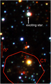 |
Fig. E.3 JHKs compositecolour image covering the centre of the C1 clump (red contour: column density 1 × 1023 cm−2) and the vicinity of our candidate exciting star. |
Coordinates of a few sources discussed in the text.
Coordinates and photometry of our candidate exciting star.
E.2 Dust temperature, column density, and molecular clumps
Figure E.4 displays the column density map of the nebula. The column density is high in the vicinity of the bipolar nebula, higher than 2 × 1022 cm−2 throughout.In particular, the column density is higher than 3.2 × 1022 cm−2 along the parental filament. Two bright clumps lie along the parental filament. They are identified as C1 and C2 in Fig. E.4 and their parameters are given in Table E.3. The clump C2 lies at the left waist of the bipolar nebula with a peak column density of 2.4 × 1023 cm−2, and C1 liesin the middle of the filament with a peak column density of 3.1 × 1023 cm−2. These clumps are adjacent to the ionised gas.
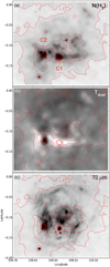 |
Fig. E.4 Column density in the vicinity of G339.58–00.12. Panel a: column density map; the red contours are for levels of 2, 3, 4, 6, 8, 10 × 1022 cm−2. Panel b: same contours superimposed on the dust temperature map. Panel c: same contours superimposed on the Herschel-70 μm image. |
Properties of the clumps in the field of G339.58–00.12.
There are two IRAS sources in the direction of this nebula. The C2 clump positionally coincides with one of the IRAS sources, IRAS 16424–4531 (coordinates: l = 339. °6201, b = –00. °1180). The other IRAS source, IRAS 16421–4532, lies near the centre of the top lobe (coordinates: l = 339. °5634, b = –00. °0909). Methanol maser emission at 6.7 GHz is observed in the direction of each of the clumps (Caswell 1996) indicating that massive-starformation is at work there.
Figure E.5 displays the dust temperature map of the G339.58–00.12 field. The temperature is low in the dust filament at the waist of the nebula, lower than 18.5 K, except in the direction of the C2 clump; a minimum temperature of 16.0 K is reached in the filament. The highest dust temperature in the field is ~ 21.2 K; it is observed in the direction of clump C2, on its side adjacent to the ionised region. The opposite side of C2 is cold, like the other parts of the parental filament. The temperature of the clump C1 is typical of that of the parental filament, in the range 16.0 K–17.0 K. There is therefore a temperature difference between the two clumps. As shown by Fig. E.5, the dust temperature in the filaments forming the northern lobe is in the range 19.5 K–20 K, and is therefore clearly higher than in the parentalfilament.
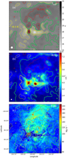 |
Fig. E.5 Dust temperature in the vicinity of G339.58–00.12. Panel a: dust temperature map; the red contours are for temperatures of 19.5 K, 20 K, and 20.5 K, the green one for 19 K, and the yellow ones for temperatures of 17.5 K, 18 K, and 18.5 K. Panel b: same contours are superimposed on the column density map. Panel c: contours are superimposed on the Spitzer 8.0 μm image. |
The two clumps are rather similar in terms of mass, size, and density (Table E.3). They are compact, with an equivalent radius in the range 0.12–0.145 pc. Their mean volume density is high, in the range 6–7 × 105 cm−3, but their stellar content possibly differs, which explains why they are so different in terms of dust temperature. Another possible explanation is that the C1 clump lies in front of the H II region and is along the line of sight, and we do not see its warm face turned towards the ionised gas.
We know that clump C2 is associated with the central H II region because the CS emission in the direction of IRAS 16424–4531 (therefore in the direction of C2) has a velocity of − 33.2 km s−1 (Bronfman et al. 1996), very similar to that of the ionised gas.
Two Class II methanol masers have been detected at 6.7 GHz in the direction of this region. Their positions are given at sub-arcsecond accuracy by Caswell (1996). The brightest maser (maser 2 in Table E.1) lies in the direction of clump C2. Its velocity is − 32.8 km s−1 (see also Walsh et al. 1998, who found seven maser points with a velocity in the range − 32.5 to − 37.8 km s−1). The other methanol maser (maser 1 in Table E.1) is fainter and lies in the direction of the C1 central clump; its velocity is − 31.3 km s−1 (Caswell 1996). The presence of an EGO (possibly a MYSO outflow candidate) is also reported by Cyganowski et al. (2008) in the direction of clump C1. An OH maser has been detected at 6 cm in the direction of the EGO with a velocity of –32 km s−1, but the resolution of the OH observations (beam of 10′) does not allow us to definitively associate it with a specific source.
E.3 Infrared dark clouds
Seven IRDCfragments are detected by Peretto & Fuller (2009). Two IRDC fragments are spatially correlated with condensations adjacent to the north-west lobe. The other five IRDCs are detected in the direction of absorption features linked to the parental filament. But once again, the brightest clump, C1, is not detected as an IRDC fragment, and the IRDC fragment detected in the vicinity of C2 is centred ~31′′ away from the Herschel column density peak.
E.4 Young stellar objects and star formation
Figure E.7 shows the [3.6]–[4.5] vs. [5.8]–[8.0] colour–colour of the point sources. The Class I YSOs and a few interesting sources are marked with different ID numbers. The astrometry and photometry of these sources are given in Table E.4.
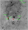 |
Fig. E.6 IRDCs detected by Peretto & Fuller (2009) in the field of G339.58–00.12 overlaid on the Spitzer 8.0 μm image. |
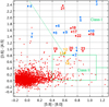 |
Fig. E.7 Colour–colour diagram, [3.6]–[4.5] vs. [5.8]–[8.0], for Spitzer-GLIMPSE sources with measurements in the four bands that are located less than 8′ from the centre of clump C1. The sources discussed in the text, mainly candidate Class I YSOs, are identified (blue, orange, and red dots indicate sources in the direction of C1, C2, and the whole bipolar nebula, respectively). |
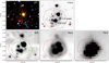 |
Fig. E.8 Sources in the direction of the C1 clump. The YSOs discussed in the text and in Table E.4 are identified on images in the NIR (JHKs colour composite image), at 4.5 μm, 8 μm, 24 μm, and 70 μm. The red contour corresponds to a column density of 1 × 1023 cm−2, and the green contour (superimposed on the 8 μm image) to a column density of 1.6 × 1023 cm−2. This latter contour follows a level that is half of the N(H2) peak’s intensity. |
Sources in the field of G339.58–00.12, mainly candidate Class I YSOs or objects discussed in the text.
The C1 clump harbours a deeply embedded cluster containing several candidate Class I YSOs. We found ten candidate Class I YSOs in the direction or vicinity of C1 (Fig. E.8); four of them (#2, #3, #4, and #6) are bright 24 μm sources, and at least two of them, #4 and #6, are strong 70 μm sources as well (they are not well-separated at the angular resolution of the 70 μm data). Sources #1, #8, and #10 are also 24 μm sources, butare faint; their [8.0]–[24] colours suggest flat-spectrum YSOs. The evolutionary stage of sources #5, #7, and #9 is more uncertain as they have no measurements at 24 μm. The faint Class II methanol maser (i.e. maser 2) lies ~0.′′6 away from source #4. The EGO detected by Cyganowski et al. (2008) lies ~0.′′3 from source #6. A 95 GHz Class I methanol maser has been detected by Chen et al. (2011) in the direction of the EGO, but the resolution of these observations(beam of 36′′) does not allow us to say whether it is associated with source #6 or source #4. Sources #2, #3, #4, and #6 at the very centre of C1 form a trapezium of candidate Class I YSOs; their [8.0]–[24] colour, higher than 3.9 mag, confirms their young evolutionary stages. YSO #4 is probably the least-evolved of them due to its [8.0]–[24] colour of 8.07 mag and its association with a Class II methanol maser. At 70 μm, the sources are not clearly separated. The whole cluster, dominated by YSOs #4 and #6, has a flux ~122 Jy at 70 μm, indicating a luminosity of ~2400L⊙.
Clump C2 contains several remarkable point sources as shown by Fig. E.9; it also contains two regions of extended diffuse emission at 8.0 μm and 24 μm. The extended regions are identified as A and B in Fig. E.9; they are discussed in E.5. At thevery centre of C2 lies a bright IR source, #11, which is saturated at Spitzer wavelengths from 3.6 μm to 24 μm. It shows somewhat extended emission in the NIR (JHKs). Its WISE photometry ([3.4] = 7.280, [4.6] = 3.299, [12] = 1.243, and [22] = –2.092 mag) is that of a candidate Class I YSO (using Koenig et al’s. criteria). It is very bright at 70 μm, with a flux ~860 Jy corresponding to a luminosity of ~15 000L⊙ (there is possibly a small contribution of sources A and B (discussed in Sect. E.5) to this flux). No UC H II region has been detected by Walsh et al. (1998) in this direction (detection limit of 1 mJy beam−1 at 8.64 GHz). The bright Class II methanol maser lies nearby, about 1′′ away from YSO #11 (Caswell 1996). Three other candidate YSOs of unknown nature lie on the border of C2; they are the sources #12, #13, and #14 of Fig. E.9. They are faint at 24 μm to be measured at this wavelength and lie too close to the bright YSO #11.
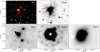 |
Fig. E.9 Sources in the vicinity of the C2 clump. As in Fig. E.8 but the green contour now corresponds to a column density of 1.26 × 1023 cm−2 (level that is half the N(H2) peak’s intensity). |
Several other sources located in the vicinity of the bipolar nebula are candidate Class I YSOs. They are identified in Fig. E.10. According to Robitaille et al. (2008), the field in Fig. E.10 (size 13.′9 × 13.′6) could contain three candidate AGB stars. Robitaille et al. (2008) propose that candidate xAGB stars have [4.5] ≤ 7.8 mag and sAGBs stars have [4.5] ≥ 7.8 and [8.0]–[24] ≤ 2.5; therefore, source #17 ([4.5] = 6.61 and [8.0]–[24] = 1.21 mag) is probably an AGB star. The nature of sources #18, #19, and #23, which are all bright at 4.5 μm, is uncertain as they could be either AGB stars or Class II YSOs. Also, we do not know if these sources are associated with the bipolar nebula. YSO #20, located in the direction of the parental filament, is probably associated with the region; its [8]–[24] colour indicates that it is probably a Class II YSO. Source #15 is located in the direction of a high-column-density feature (3.4 × 1022 cm−2) that appearsin absorption at 8.0 μm and 24 μm, and lies at the border of the top lobe of the bipolar nebula. It is only detected at 70 μm, and is therefore possibly a very young YSO with a low luminosity ( ~3L⊙).
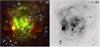 |
Fig. E.10 Sources in the G339.58–00.12 field (except in C1 and C2). Panel a: colour image with red, green, and blue indicating the 70 μm, 24 μm, and 4.5 μm images, respectively. Panel b: sources are identified on the Hi-GAL 70 μm image. |
A small clump (at l = 339. °634, b = –00. °176 with a peak column density of ~5.6 × 1022 cm−2) lies outside the bottom lobe, almost adjacent to it. In this direction lies YSO #21, which is probably a Class I YSO according to its [8]–[24] colour. It is a bright source at 70 μm and its flux indicates a luminosity of about 1500L⊙ if at a distance of 2.8 kpc, but its association with the bipolar nebula is uncertain. Near YSO #21 lies YSO #22, which is probably a flat spectrum YSO, and #23, which is of uncertain nature (Class II YSO or AGB star).
E.5 Small regions of extended diffuse IR emission
A number of small diffuse emission regions are observed from 8.0 μm to 70 μm. They are identified as regions of A, B and C in Fig. E.10 and their parameters are given in Table E.5. Regions A and B are located in the direction of C2, at 0.25 pc and 0.21 pc from the bright YSO #11, respectively (Fig. E.9). A star lies in the centre of region B; its VISTA photometry (H = 17.741 and Ks =15.059 magnitude) is compatible with an early B star (B2V or B3V), with an extinction of ~40 mag if at a distance of 2.8 kpc. This star is possibly the main heating source of the dust in this region. The star at the centre of region A is only detected in Ks data, and therefore its photometric spectral type could not be estimated. Regions A and B lie too close to YSO #11, and therefore are not measurable at 70 μm.
Small regions of extended emission present in the field of G339.58–00.12.
Region C lies south of the clump C1, ~0.53 pc from the column density peak of C1. A star lies at the centre of region C; its VISTA photometry (J = 16.138, H = 14.219, and K = 13.093 mag) is compatible with a B3V star affected by a visual extinction ~18 mag if at 2.8 kpc. Therefore, this star is possibly the heating source of the dust in Region C. The 70 μm flux of the region C, however, corresponds to a luminosity ~280L⊙, which is too low for an early B star.
Region D lies in the middle of the top lobe. It is bright at 70 μm and its flux corresponds to a luminosity of ~1500L⊙. At 250 μm, a point source appears adjacent to region D. The mass of the clump or envelope surrounding region D is ~45 ± 3 M⊙.
Appendix F G342.07+00.42
The H II region G342.07+00.42 is composedof three bubbles from the Churchwell et al. (2006) catalogue: S18, S19, and S20 (Fig. F.1). We propose that they are part of a bipolar H II region. Our arguments are the followings: i) A dense filament is observed at all SPIRE wavelengths and is easily seen on the column density map (Fig. F.1b). ii) Two lobes are present, perpendicular to the filament; one lobe corresponds to the S18 bubble, the other one is formed by the S19 and S20 bubbles. This latter lobe highly resembles the bottom lobe in Sh 201 (Deharveng et al. 2012). We suggest that the out-flowing ionised gas interacts with a pre-existing condensation on its way. The lobe is distorted and seems to split into two pieces (the S19 and S20 bubbles). iii) There is only one main extended region of 24 μm emission (this emission is saturated in the very centre), which lies along the filament, near the centre of the bipolar structure (Fig. F.1a). No strong Hα emission is found to be associated with the H II region. The Hα SuperCOSMOS image shows extended diffuse emission, and large absorption zones without any correlation with the distribution of cold dust.According to Georgelin et al. (1996) the G342.07+00.42 H II region is hidden behind the large and nearby RCW 113 H II region (which lies at about 2 kpc).
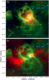 |
Fig. F.1 Bipolar nebula G342.07+00.42. Panel a: composite colour image as seen by Spitzer, and identification of the S18, S19, and S20 bubbles. Red, green, and blue are for the 24 μm, 8.0 μm, and 4.5 μm emissions, respectively (note that the 24 μm image is saturated in the central region). Panel b: red channel now shows the column density of molecular hydrogen. |
F.1 Distanceand exciting star
Caswell & Haynes (1987) measured an integrated flux density of 3.30 Jy at 5 GHz, and a velocity of − 65 km s−1 for the ionised gas; they estimated the kinematic distance to be 5.7 kpc or 13.3 kpc. Kuchar & Clark (1997) measured a peak flux density of 3.85 Jy at 4.85 GHz. Georgelin et al. (1996) suggest the existence of a spiral arm at about 5 kpc, and propose a distance of 4.7 kpc for G342.07+00.42. Anderson et al. (2014) in their WISE catalogue of Galactic H II regions give a distance of 4.7 ± 0.4 kpc, based on the velocity of the ionised gas and on the velocity of the H i absorption line. We adopt this distance of 4.7 kpc in the following.
No exciting star has been identified in this region. Adopting a radio flux at 5 GHz of 3.8 Jy, an electron temperature of 8000 K, and a distance of 4.7 kpc, we estimate the ionising flux NLyc in s−1, which points to an exciting star of spectral type O5.5V–O6V.
As shown by Fig. F.2, a cluster is present at the centre of the field. The cluster is reported by Dutra et al. (2003) and lies at l = 342. °069, b = +00. °417, which is the location between two dense clumps, C1 and C2, observed at the waist of the nebula (clumps are discussed in Sect. F.2). Furthermore, the VISTA survey images show the presence of a compact, highly reddened cluster in the direction of C2. We use data from the 2MASS and VISTA catalogues to study these clusters. Figure F.3 displays the J vs. J − K diagram of the stars located at less than 90′′ from the centre ofthe 24 μm saturated region (coordinates: l = 342. °0611, b = +00. °4196). The bright stars discussed in the paper are identified in Figs. F.2 and F.3. Figure F.3 suggests that: i) the two bright stars #7 and #19 are too bright to be related to the region. Other stars could also be foreground stars, but they are not easy to identify; ii) the locus of OV stars at a distance of 4.7 kpc is shown with blue plus symbols and the area located between the two slanted extinction lines contains several such stars. These stars possibly participate in the ionisation of the H II region. The main candidates appear to be stars #8, #15, and #11. The J − K colour of #8 (if an O star) indicates a visual extinction ~18.0 ± 2.0 mag; the extinction of #11 seems to be ~25.5 ± 2.0 mag. Although stars #8 and #11 are more massive than an O5V star, star #11 is a YSO according its NIR colours. Moreover, it lies close ( ~6.6′′ away) to a UC H II region G342.0610+00.4200 (Urquhart et al. 2007) and therefore is probably not the main exciting star of the nebula; it instead seems to be part of the compact cluster located in the direction of C2. We believe either star #8 or #15 is responsible for the majority of the ionisation of the nebula. The distance of the region is possibly overestimated for star #8; if it is an O5V star then it should at a distance of 4.1 ± 1.0 kpc. Star #15 lies at the centre of a small 8 μm cavity located between C1 and C2, and if it is at 4.7 kpc, then its spectral type is O5.5V, consistent with the spectral type obtained from radio measurements. Stars #3, #16, and #20 could also contribute to the ionisation, but being of O9.5V-type, their contribution should be less. Stars such as #5, #22, #13, #14, and #9 are possibly part of the cluster; and iii) Star #23 shows a visual extinction much smaller than that of the stars quoted before. It is also located behind the PAHs bright rim tracing the IF of the H II region (therfore outside the ionised region), at the east waist of the nebula. This suggests that star #23 is located in front of the nebula and is possibly a foreground star. Like star #23, several other stars (stars #17, #12, #24, #1, #4, etc.) show a visual extinction smaller than 10 mag. These stars are most likely foreground stars and are therefore not associated with the nebula.
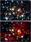 |
Fig. F.2 Exciting cluster of G342.07+00.42. Panel a: colour image with J, H, K, in blue, green, and red, respectively. Panel b: colour image with J, K, and 3.6 μm emission in blue, green, and red, respectively. Sources discussed in the text are identified. The main candidate exciting star is #8. The red contours are for column densities of 4, 6, and 8 × 1022 cm−2. |
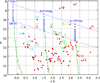 |
Fig. F.3 J vs. J − K diagram of the stars in the central region of G342.07+00.42. Their magnitudes are from the 2MASS and VISTA catalogues; we do not use VISTA data for stars brighter than 12.5 mag in J and K and 13.0 mag in H as they are probably saturated. The main sequence for OV stars is from Martins & Plez (2006), for visual extinctions of 0 mag, 20 mag, and 40 mag, and assuming a distance of 4.7 kpc; the extinction law is that of Rieke & Lebofsky (1985). The 2MASSphotometry of highly reddened stars must be regarded with caution as shown by the discrepancy between the 2MASS and VISTA measurements of some stars (joined by black lines). The stars are identified by their numbers according toFig. F.2. |
F.2 Dust temperature, column density and clumps
Figure F.4 shows the column density map of the G342.07+00.42 nebula. Four bright clumps, C1 to C4, lie in the direction of this nebula. Among the clumps, C1 and C2 are compact and dense. Their coordinates and parameters are given in Table F.2 and their positions are also shown in Fig. F.4. The column density is higher than 1 × 1022 cm−2 throughout; it reaches 2.1 × 1023 cm−2 in C1, the clump located on the western side of the bipolar nebula, and 1 × 1023 cm−2 in C2, the more extended condensation located at the eastern side at the waist of the bipolar nebula.
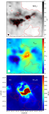 |
Fig. F.4 Column density of the neutral material in the vicinity of G342.07+00.42. The contours correspond to column densities of 2, 4, 6, 8, and 10 × 1022 cm−2. They are superimposed on the column density map (panel a), temperature map (panel b), and Herschel 70 μm map (panel c). The clumps C1 to C4 discussed in the text are identified. |
Exciting star(s) of G319.88+00.79.
Molecular clumps in the field of G342.07+00.42.
Figure F.5 shows the dust temperature map of the nebula. Low values are observed in the direction of the parental filament ( ≤17 K), on each side of the ionised region. The lowest temperature (14.5 K) is found in the direction of clump C2. Higher temperatures are observed in the direction of the ionised region and its PDR, up to 21.5 K. The temperature is slightly lower in the direction of the bright clump C1 ( ~19.5 K); but the low resolution of the map and the nearby ionised zone prevent any accurate temperature measurement for this structure. Figure F.5c presents a clear correlation between the zone of warm dust and the zone of PAH emission.
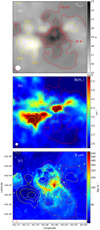 |
Fig. F.5 Dust temperature in the vicinity of G342.07+00.42. The red contours are for temperatures of 18.5 K, 19 K, 19.5 K, 20 K, and 20.5 K, the yellow ones for 15 K, 16 K, and 17 K. These curves are superimposed on the temperature map (panel a), the column density map (panel b), and the Spitzer 8.0 μm map (panel c). |
Three clumps (C1, C2, and C3) are observed along the parental filament. Among these clumps, clump C1 is remarkable for its mass ( ~1000 M⊙) and density (3 × 10⁵) in its central region; it is relatively circular with an equivalent radius of 0.23 pc.
This region is also the site of an IRAS source, IRAS 16489-4318 (coordinates: l = 342. °063, b = +00. °420), that lies on the border of a bright clump C1 (located between stars #11 and #12; Fig. F.2). We turn to MALT90 observations(details about MALT90 data can be found in Paper I) to examine the association of the clumps with the nebula. The HCO+ (1–0) and HNC (1–0) lines are used. They indicate velocities in the range –69 km s−1 to –76 km s−1 in the whole region. The central parts of C1 have a velocity in the range –69.5 km s−1 to –73.0 km s−1, in relatively good agreement with the velocity of the ionised gas. The more extended C2 condensation has a velocity in the range –70 km s−1 to –75 km s−1. The C3 and C4 clumps (see Fig. F.4) have velocities of ~ –73 km s−1 and ~ 77 km s−1, respectively.In conclusion, MALT90 observations show that the molecular material in the parental filament and surrounding the bipolar H II region is associated with this region.
F.3 Infrared dark clouds
Peretto & Fuller (2009) reported the presence of seven IRDC fragments in the direction or vicinity of G342.07+00.42. Their locations are shown in Fig. F.6. Two of them (SDC G342.036+00.434 and G342.103+00.404 in clumps C3 and C2, respectively) correspond to dense extended structures on each side at the waist of the nebula. Two others (SDC G342.067+0.437 and SDC G342.092+0.449) correspond to smaller features seen in absorption in the direction of the top lobe. Three of them (SDC G342.081+0.432 and SDC G342.068+0.452 inside of S18, and SDC G342.073+00.390 in the centre of S19) are not real structures but zones surrounded by bright 8 μm emission filaments. The most massive and compact clump (C1), which however displays absorption features at 8.0 μm, is not identified as an IRDC by Peretto & Fuller (2009).
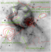 |
Fig. F.6 IRDC fragments identified by Peretto & Fuller (2009) in the field of G342.07+00.42. The underlying grey image is the Spitzer 8.0 μm image. The red contours correspond to column densities of 2, 4, 6, 8, and 10 × 1022 cm−2. |
F.4 Young stellar objects and star formation
We do not present the [3.6]–[4.5] vs. [5.8]–[8.0] diagram used to select candidate Class I YSOs, as very few candidates are found in this field. The point sources identified as YSOs based on the GLIMPSE colours and/or [8]–[24] colours are identified in Fig. F.7.
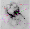 |
Fig. F.7 Spatial distributions of Class I (red circles), Flat (cyan circles), and Class II (green circle) on the 8.0 μm image. The contours correspond to column densities of 2, 4, 6, 8, and 10 × 1022 cm−2. The positions of the MYSO and EGO are also shown. |
As can be seen from Fig. F.7, a Class I YSO lies at the centre of the nebula. This is our star #15, one of the potential ionising sources of the nebula. We do not agree with its Class I YSO classification. At 24 μm, star #15 shows extended emission. We believe that the background emission from warm dust has contaminated the measurement of the 24 μm flux, resulting an excess flux at 24 μm.
Two Class I YSOs are located at the border of the top lobe. These YSOs are quite faint at 8.0 μm, and therefore their evolutionary statuses are also uncertain. In the direction of G342.07+00.42, an EGO, a “possible MYSO outflow candidate” is reported by Cyganowski et al. (2008); it lies at the border of a small extended emission region near the waist of the nebula, but outside it. A MSYO, in terms of UC H II region has also been identified in the direction of C1 (see discussion in Sect. F.1). The locations of the EGO and the MYSO are also shown in Fig. F.7. Here again, the most massive YSO and clump lie at the waist of the nebula.
References
- Acker, A., Chopinet, M., Pottash, S. R., & Stenholm, B. 1987, A&AS, 71, 163 [NASA ADS] [Google Scholar]
- Allen, L. E., Calvet, N., D’Alessio, P., et al. 2004, ApJS, 154, 363 [NASA ADS] [CrossRef] [Google Scholar]
- Anathpindika, S., & Freundlich, J. 2015, PASA, 32, e007 [NASA ADS] [CrossRef] [Google Scholar]
- Anderson, L. D., Bania, T. M., Balser, D. S., & Rood, R. T. 2011, ApJS, 194, 32 [NASA ADS] [CrossRef] [Google Scholar]
- Anderson, L. D., Bania, T. M., Balser, D. S., & Rood, R. T. 2012, ApJ, 754, 62 [NASA ADS] [CrossRef] [Google Scholar]
- Anderson, L. D., Bania, T. M., Balser, D.S., et al. 2014, ApJS, 212, 1 [NASA ADS] [CrossRef] [Google Scholar]
- Anderson, L. D., Hough, L. A., Wenger, T. V., et al. 2015, ApJ, 810, 42 [NASA ADS] [CrossRef] [Google Scholar]
- André, P., Men’shchikov, A., Bontemps, S., et al. 2010, A&A, 518, L102 [NASA ADS] [CrossRef] [EDP Sciences] [Google Scholar]
- André, P., Di Francesco, J., Ward-Thompson, D., et al. 2014, Protostars and Planets VI (Arizona: University of Arizona Press), 27 [Google Scholar]
- Arthur, S. J., & Hoare, M. G. 2006, ApJS, 165, 283 [NASA ADS] [CrossRef] [Google Scholar]
- Arzoumanian, D., Andrè, Ph., Didelon, P., et al. 2010, A&A, 529, L6 [Google Scholar]
- Avedisova, V. S., & Kondratenko, G. I. 1984, Ninfo, 56, 59 [Google Scholar]
- Baldeschi, A., Molinari, S., Elia, D., Pezzuto, S., & Schisano, E. 2017, MNRAS, 472, 1778 [NASA ADS] [CrossRef] [Google Scholar]
- Bally, J., Snell, R. L., & Predmore, R. 1983, ApJ, 272, 154 [NASA ADS] [CrossRef] [Google Scholar]
- Bania, T. M., Anderson, L. D., Balser, D. S., & Rood, R. T. 2010, ApJ, 718, L106 [NASA ADS] [CrossRef] [Google Scholar]
- Beaumont, C. N., & Williams, J. P. 2010, ApJ, 709, 791 [NASA ADS] [CrossRef] [Google Scholar]
- Bernard, A., Neichel, B., Samal, M. R., et al. 2016, A&A, 592, A77 [NASA ADS] [CrossRef] [EDP Sciences] [Google Scholar]
- Bica, E., Dutra, C. M., Soares, J., & Barbuy, B. 2003, A&A, 404, 223 [NASA ADS] [CrossRef] [EDP Sciences] [Google Scholar]
- Bieging, J. H., Peters, W. L., & Kang, M. 2010, ApJS, 191, 232 [NASA ADS] [CrossRef] [Google Scholar]
- Bik, A., Kaper, L., Hanson, M. M., & Smits, M. 2005, A&A, 440, 121 [NASA ADS] [CrossRef] [EDP Sciences] [Google Scholar]
- Bodenheimer, P., Tenorio-Tagle, G., & Yorke, H. W. 1979, ApJ, 233, 85 [NASA ADS] [CrossRef] [Google Scholar]
- Breen, S. L., Ellingsen, S. P., Caswell, J. L., & Lewis, B. E. 2010, MNRAS, 401, 2219 [NASA ADS] [CrossRef] [Google Scholar]
- Bronfman, L., Nyman, L.-A., & May, J. 1996, A&AS, 115, 81 [NASA ADS] [Google Scholar]
- Busfield, A. L., Purcell, C. R., Hoare, M. G., et al. 2006, MNRAS, 366, 1096 [NASA ADS] [CrossRef] [Google Scholar]
- Carey, S. J., Noriega-Crespo, A., Mizuno, D. R., et al. 2009, PASP, 121, 76 [NASA ADS] [CrossRef] [Google Scholar]
- Caswell, J. L. 1996, MNRAS, 279, 79 [NASA ADS] [CrossRef] [Google Scholar]
- Caswell, J. L. 1998, MNRAS, 297, 215 [NASA ADS] [CrossRef] [Google Scholar]
- Caswell, J. L. 2001, MNRAS, 326, 805 [NASA ADS] [CrossRef] [Google Scholar]
- Caswell, J. L., & Haynes, R. F. 1987, A&A, 171, 261 [NASA ADS] [Google Scholar]
- Caswell, J. L., Batchelor, R. A., Forster, J. R., & Wellington, K. J. 1989, Austr. J. Phys., 42, 331 [NASA ADS] [CrossRef] [Google Scholar]
- Caswell, J. L., Vaile, R. A., Ellingsen, S. P., et al. 1995a, MNRAS, 272, 96 [NASA ADS] [CrossRef] [Google Scholar]
- Caswell, J. L., Vaile, R. A., Ellingsen, S. P., & Norris, R. P. 1995b, MNRAS, 274, 1126 [NASA ADS] [Google Scholar]
- Chen, X., Ellingsen, S. P., Shen, Z.-Q., et al. 2011, ApJS, 196, 9 [NASA ADS] [CrossRef] [Google Scholar]
- Churchwell, E., Povich, M. S., Allen, D., et al. 2006, ApJ, 649, 7597 [NASA ADS] [CrossRef] [Google Scholar]
- Churchwell, E., Watson, D. F., Povich, M. S., et al. 2007, ApJ, 670, 428 [NASA ADS] [CrossRef] [Google Scholar]
- Culverhouse, T., Ade, P., Bock, J., et al. 2011, ApJS, 195, 8 [NASA ADS] [CrossRef] [Google Scholar]
- Cyganowski, C. J., Whitney, B. A., Holden, E., et al. 2008, AJ, 136, 2391 [NASA ADS] [CrossRef] [Google Scholar]
- Cyganowski, C. J., Koda, J., Rosolowsky, E., et al. 2013, ApJ, 764, 61 [NASA ADS] [CrossRef] [Google Scholar]
- Dale, J. E., Bonnell, I. A., & Whitworth, A. P. 2007, MNRAS, 375, 1291 [NASA ADS] [CrossRef] [Google Scholar]
- Dale, J. E., Haworth, T. J., & Bressert, E. 2015, MNRAS, 450, 1199 [NASA ADS] [CrossRef] [Google Scholar]
- Deharveng, L., Schuller, F., Anderson, L. D., et al. 2010, A&A, 523, A6 [NASA ADS] [CrossRef] [EDP Sciences] [Google Scholar]
- Deharveng, L., Zavagno, A., Anderson, L. D., et al. 2012, A&A, 546, A74 [NASA ADS] [CrossRef] [EDP Sciences] [Google Scholar]
- Deharveng, L., Zavagno, A., Samal, M.R., et al. 2015, A&A, 582, A1 (Paper I) [NASA ADS] [CrossRef] [EDP Sciences] [Google Scholar]
- de Geus, E. J., Bronfman, L., & Thaddeus, P. 1990, A&A, 231, 137 [NASA ADS] [Google Scholar]
- Dobashi, K. 2011, PASJ, 63, 1 [NASA ADS] [CrossRef] [Google Scholar]
- Dunham, M. M., Crapsi, A., Evans, N. J., et al. 2008, ApJS, 179, 249 [NASA ADS] [CrossRef] [Google Scholar]
- Dutra, C., & Bica, E. 2002, A&A, 383, 631 [NASA ADS] [CrossRef] [EDP Sciences] [Google Scholar]
- Dutra, C. M., Bica, E., Soares, J., & Barbuy, B. 2003, A&A, 400, 533 [NASA ADS] [CrossRef] [EDP Sciences] [Google Scholar]
- Dyson, J. E., & Williams, D. A. 1997, in The Physics of the Interstellar Medium, 2nd ed. (Bristol: Institute of Physics Publishing) [CrossRef] [Google Scholar]
- Ellsworth-Bowers, T. P., Rosolowsky, E., Glenn, J., et al. 2015, ApJ, 799, 29 [NASA ADS] [CrossRef] [Google Scholar]
- Eswaraiah, C., Lai, S.-P., Chen, W.-P., et al. 2017, ApJ, 850, 195 [NASA ADS] [CrossRef] [Google Scholar]
- Fontani, F., Cesaroni, R., & Furuya, R. S. 2010, A&A, 517, A56 [NASA ADS] [CrossRef] [EDP Sciences] [Google Scholar]
- Foster, J. B., Jackson, J. M., Barnes, P. J., et al. 2011, ApJS, 197, 25 [NASA ADS] [CrossRef] [Google Scholar]
- Foster, J. B., Rathborne, J. M., Sanhueza, P., et al. 2013, PASA, 30, e038 [NASA ADS] [CrossRef] [Google Scholar]
- Franco, J., Tenorio-Tagle, G., & Bodenheimer, P. 1990, ApJ, 349, 126 [NASA ADS] [CrossRef] [Google Scholar]
- Fukuda, N., & Hanawa, T. 2000, ApJ, 533, 911 [NASA ADS] [CrossRef] [Google Scholar]
- Gardner, F. F., & Whiteoak, J. B. 1978, MNRAS, 183, 711 [NASA ADS] [CrossRef] [Google Scholar]
- Georgelin, Y. M., Boulesteix, J., Georgelin, Y. P., et al. 1987, A&A, 174, 257 [NASA ADS] [Google Scholar]
- Georgelin, Y. M., Russeil, D., Marcelin, M., et al. 1996, A&AS, 120, 41 [NASA ADS] [CrossRef] [EDP Sciences] [Google Scholar]
- Goedhart, S., Gaylard, M. J., & van der Walt, D. J. 2004, MNRAS, 355, 553 [NASA ADS] [CrossRef] [Google Scholar]
- Goldsmith, P. F., Heyer, M., Narayanan, G., et al. 2008, ApJ, 680, 428 [NASA ADS] [CrossRef] [Google Scholar]
- Green, J. A., & McClure-Griffiths, N. M. 2011, MNRAS, 417, 2500 [NASA ADS] [CrossRef] [Google Scholar]
- Green, J. A., Caswell, J. L., Fuller, G. A., et al. 2010, MNRAS, 409, 913 [NASA ADS] [CrossRef] [Google Scholar]
- Gvaramadze, V. V., Kniazev, A. Y., & Fabrika, S. 2010, MNRAS, 405, 1047 [NASA ADS] [Google Scholar]
- Hartley, M., Tritton, S. B., Manchester, R. N., et al. 1986, A&AS, 63, 27 [NASA ADS] [Google Scholar]
- Helfand, D. J., Becker, R. H., White, R. L., Fallon, A., & Tuttle, S. 2006, AJ, 131, 2525 [NASA ADS] [CrossRef] [Google Scholar]
- Henney, W. J., Arthur, S. J., & García-Díaz, M. T. 2005, ApJ, 627, 813 [NASA ADS] [CrossRef] [Google Scholar]
- Hill, T., Motte, F., Didelon, P., et al. 2011, A&A, 533, A94 [NASA ADS] [CrossRef] [EDP Sciences] [Google Scholar]
- Hosokawa, T., & Inutsuka, S.-I. 2005, ApJ, 623, 917 [NASA ADS] [CrossRef] [Google Scholar]
- Huang, M., Bania, T. M., Bolatto, A., et al. 1999, ApJ, 517, 282 [NASA ADS] [CrossRef] [Google Scholar]
- Hughes, V. A., & MacLeod, G. C. 1994, ApJ, 427, 857 [NASA ADS] [CrossRef] [Google Scholar]
- Indebetouw, R., Mathis, J. S., Babler, B. L., et al. 2005, ApJ, 619, 931 [NASA ADS] [CrossRef] [Google Scholar]
- Jackson, J. M., Finn, S. C., Rathborne, J. M., et al. 2008, ApJ, 680, 349 [NASA ADS] [CrossRef] [Google Scholar]
- Jackson, J. M., Rathborne, J. M., Foster, J. B., et al. 2013, PASA, 30, e057 [NASA ADS] [CrossRef] [Google Scholar]
- Kahn, F. D., & Dyson, J. E. 1965, ARA&A, 3, 47 [NASA ADS] [CrossRef] [Google Scholar]
- Kang, M., Bieging, J. H., Povich, M. S., & Lee, Y. 2009, ApJ, 706, 83 [NASA ADS] [CrossRef] [Google Scholar]
- Koenig, X. P., Leisawitz, D. T., Benford, D. J., et al. 2012, ApJ, 744, 130 [NASA ADS] [CrossRef] [Google Scholar]
- Könyves, V., André, P., Men’shchikov, A., et al. 2015, A&A, 584, A91 [NASA ADS] [CrossRef] [EDP Sciences] [Google Scholar]
- Kothes, R., & Dougherty, S. 2007, A&A, 468, 993 [NASA ADS] [CrossRef] [EDP Sciences] [Google Scholar]
- Kothes, R., & Dougherty, S. 2008, Rev. Mex. Astron. Astrof., 33, 163 [NASA ADS] [Google Scholar]
- Kuchar, T. A., & Clark, F. O. 1997, ApJ, 488, 224 [NASA ADS] [CrossRef] [Google Scholar]
- Lawrence, A., Warren, S. J., Almaini, O., et al. 2007, MNRAS, 379, 1599 [NASA ADS] [CrossRef] [MathSciNet] [Google Scholar]
- Lee, E. J., Murray, N., & Rahman, M. 2012, ApJ, 752, 146 [NASA ADS] [CrossRef] [Google Scholar]
- Liu, H.-L., Li, J.-Z., Wu, Y., et al. 2016, ApJ, 818, 95 [NASA ADS] [CrossRef] [Google Scholar]
- Lockman, F. J. 1989, ApJS, 71, 469 [NASA ADS] [CrossRef] [Google Scholar]
- Longmore, S. N., Burton, M. G., Barnes, P. J., et al. 2007, MNRAS, 379, 535 [NASA ADS] [CrossRef] [Google Scholar]
- Martins, F., & Plez, B. 2006, A&A, 457, 637 [NASA ADS] [CrossRef] [EDP Sciences] [Google Scholar]
- Martins, F., Schaerer, D., & Hillier, D. J. 2005, A&A, 436, 1049 [NASA ADS] [CrossRef] [EDP Sciences] [Google Scholar]
- Marsh, K. A., Kirk, J. M., André, P., et al. 2016, MNRAS, 459, 342 [NASA ADS] [CrossRef] [Google Scholar]
- Mc Gee, R. X., & Newton, L. M. 1981, MNRAS, 196, 889 [NASA ADS] [CrossRef] [Google Scholar]
- Megeath, S. T., Allen, L. E., Gutermuth, R. A., et al. 2004, ApJS, 154, 367 [NASA ADS] [CrossRef] [Google Scholar]
- Mercer, E. P., Clemens, D. P., Meade, M. R., et al. 2005, ApJ, 635, 560 [NASA ADS] [CrossRef] [Google Scholar]
- Minier, V., Tremblin, P., Hill, T., et al. 2013, A&A, 550, A50 [NASA ADS] [CrossRef] [EDP Sciences] [Google Scholar]
- Minniti, D., Lucas, P. W., Emerson, J. P., et al. 2010, New Astron., 15, 433 [Google Scholar]
- Mizuno, A., Onishi, T., Yonekura, Y., et al. 1995, ApJ, 445, L161 [NASA ADS] [CrossRef] [Google Scholar]
- Molinari, S., Swinyard, B., Bally, J., et al. 2010a, PASP, 122, 314 [NASA ADS] [CrossRef] [Google Scholar]
- Molinari, S., Swinyard, B., Bally, J., et al. 2010b, A&A, 518, L100 [NASA ADS] [CrossRef] [EDP Sciences] [Google Scholar]
- Molinari, S., Schisano, E., Faustini, F., et al. 2011, A&A, 530, A133 [NASA ADS] [CrossRef] [EDP Sciences] [Google Scholar]
- Motte, F., Bontemps, S., & Louvet, F. 2018, ARA&A, in press [Google Scholar]
- Myers, P. C. 2009, ApJ, 700, 1609 [NASA ADS] [CrossRef] [EDP Sciences] [Google Scholar]
- Nowak, M., Flagey, N., & Noriega-Crespo, A. 2014, ApJ, 796, 116 [NASA ADS] [CrossRef] [Google Scholar]
- Oliveira, I., Merín, B., Pontoppidan, K. M., et al. 2009, ApJ, 691, 672 [NASA ADS] [CrossRef] [Google Scholar]
- Otrupek, R. E., Hartley, M., & Wang, J.-S. 2000, PASA, 17, 92 [NASA ADS] [CrossRef] [Google Scholar]
- Panwar, N., Samal, M. R., Pandey, A. K., et al. 2017, MNRAS, 468, 2684 [NASA ADS] [CrossRef] [Google Scholar]
- Parker, Q. A., Phillipps, S., Pierce, M. J., et al. 2005, MNRAS, 362, 689 [NASA ADS] [CrossRef] [Google Scholar]
- Pavlyuchenkov, Y. N., Kirsanova, M. S., & Wiebe, D. S. 2013, Astron. Rep., 57, 573 [NASA ADS] [CrossRef] [Google Scholar]
- Pecaut, M. J., & Mamajek, E. E. 2013, ApJS, 208, 9 [Google Scholar]
- Pecaut, M. J., Mamajek, E. E., & Bubar, E. J. 2012, ApJ, 746, 154 [NASA ADS] [CrossRef] [Google Scholar]
- Peretto, N., & Fuller, G.A. 2009, A&A, 505, 405 [NASA ADS] [CrossRef] [EDP Sciences] [Google Scholar]
- Raga, A. C., Cantó, J., & Rodríguez, L. F. 2012, MNRAS, 419, L39 [NASA ADS] [CrossRef] [Google Scholar]
- Ragan, S., Henning, T., Krause, O., et al. 2012, A&A, 547, A49 [NASA ADS] [CrossRef] [EDP Sciences] [Google Scholar]
- Rieke, G. H., & Lebofsky, M. J., & Low, F. J. 1985, AJ, 90, 900 [NASA ADS] [CrossRef] [Google Scholar]
- Robitaille, T. P., Meade, M. R., Babler, B. L., et al. 2008, AJ, 136, 2413 [NASA ADS] [CrossRef] [Google Scholar]
- Rodgers, A. W., Campbell, C. T., & Whiteoak, J. B. 1960, MNRAS, 121, 103 [NASA ADS] [CrossRef] [Google Scholar]
- Romero, G. A., Schreiber, M. R., Cieza, L. A., et al. 2012, ApJ, 749, 79 [NASA ADS] [CrossRef] [Google Scholar]
- Samal, M. R., Zavagno, A., Deharveng, L., et al. 2014, A&A, 566, A122 [NASA ADS] [CrossRef] [EDP Sciences] [Google Scholar]
- Schneider, S., & Elmegreen, B. G. 1979, ApJS, 41, 87 [NASA ADS] [CrossRef] [Google Scholar]
- Schutte, A. J., van der Walt, D. J., Gaylard, M. J., & MacLeod, G. C. 1993, MNRAS, 261, 783 [NASA ADS] [CrossRef] [Google Scholar]
- Shaver, P. A., Retallack, D. S., Wamsteker, W., & Danks, A. C. 1981, A&A, 102, 225 [NASA ADS] [Google Scholar]
- Simpson, J. P., & Rubin, R. H. 1990, ApJ, 354, 165 [NASA ADS] [CrossRef] [Google Scholar]
- Simpson, R. J., Povich, M. S., Kendrew, S., et al. 2012, MNRAS, 424, 2442 [NASA ADS] [CrossRef] [Google Scholar]
- Smith, L.J., Norris, R. P. F., & Crowther, P. A. 2002, MNRAS, 337, 1309 [NASA ADS] [CrossRef] [Google Scholar]
- Skrutskie, M. F., Cutri, R. M., Stiening, R., et al. 2006, AJ, 131, 1163 [NASA ADS] [CrossRef] [Google Scholar]
- Steggles, H. G., Hoare, M. G., & Pittard, J. M. 2017, MNRAS, 466, 4573 [NASA ADS] [CrossRef] [Google Scholar]
- Strömgren, B. 1939, ApJ, 89, 526 [NASA ADS] [CrossRef] [Google Scholar]
- Stutz, A. M., Tobin, J. J., Stanke, T., et al. 2013, ApJ, 767, 36 [NASA ADS] [CrossRef] [Google Scholar]
- Tenorio-Tagle,G. 1979, A&A, 71, 59 [Google Scholar]
- Tremblin, P., Anderson, L. D., Didelon, P., et al. 2014, A&A, 568, A4 [NASA ADS] [CrossRef] [EDP Sciences] [Google Scholar]
- Tu, X., & Wang, Z.-X. 2013, Res. Astron. Astrophys., 13, 323 [NASA ADS] [CrossRef] [Google Scholar]
- Urquhart, J. S., Busfield, A. L., Hoare, M. G., et al. 2007, A&A, 461, 11 [NASA ADS] [CrossRef] [EDP Sciences] [Google Scholar]
- Vig, S., Ghosh, S. K., Ojha, D. K., & Verma, R.P. 2007, A&A, 463, 175 [NASA ADS] [CrossRef] [EDP Sciences] [Google Scholar]
- Vilas-Boas, J. W. S., & Abraham, Z. 2000, A&A, 355, 1115 [NASA ADS] [Google Scholar]
- Walch, S., Whitworth, A. P., Bisbas, T. G., Hubber, D. A., & Wünsch, R. 2015, MNRAS, 452, 2794 [NASA ADS] [CrossRef] [Google Scholar]
- Walsh, A. J., Hyland, A. R., Robinson, G., & Burton, M.G. 1997, MNRAS, 291, 261 [CrossRef] [Google Scholar]
- Walsh, A. J., Burton, M. G., Hyland, A. R., & Robinson, G. 1998, MNRAS, 301, 640 [NASA ADS] [CrossRef] [Google Scholar]
- Wang, S., Gao, J., Jiang, B. W., et al. 2013, ApJ, 773, 30 [NASA ADS] [CrossRef] [Google Scholar]
- Wang, K., Testi, L., Ginsburg, A., et al. 2015, MNRAS, 450, 4043 [NASA ADS] [CrossRef] [MathSciNet] [Google Scholar]
- Wareing, C. J., Pittard, J. M., & Falle, S. A. E. G. 2017, MNRAS, 465, 2757 [NASA ADS] [CrossRef] [Google Scholar]
- Wareing, C. J., Pittard, J. M., Wright, N. J., & Falle, S. A. E. G. 2018, MNRAS, 475, 3598 [NASA ADS] [CrossRef] [Google Scholar]
- Whiteoak, J. B., Otrupcek, R. E., & Rennie, C. J. 1982, PASAu, 4, 434 [NASA ADS] [CrossRef] [Google Scholar]
- Whitworth, A. P., Bhattal, A. S., Chapman, S. J., Disney, M. J., & Turner, J. A. 1994, MNRAS, 268, 291 [NASA ADS] [CrossRef] [Google Scholar]
- Whitworth, A., Lomax, O., Balfour, S., et al. 2018, PASJ, 70, S.55 [NASA ADS] [CrossRef] [Google Scholar]
- Wilson, T. L., Mezger, P. G., Gardner, F. F., & Milne, D. K. 1970a, A&A, 6, 364 [NASA ADS] [Google Scholar]
- Wilson, T. L., Mezger, P. G., Gardner, F. F., & Milne, D. K. 1970b, A&A, 6, 384 [Google Scholar]
- Wray, J.D. 1966, PhD dissertation, Northwestern University, IL, USA [Google Scholar]
- Wright, E. L., Eisenhardt, P. R. M., Mainzer, A. K., et al. 2010, AJ, 140, 1868 [Google Scholar]
- Xu, J.-L., Yu, N., Zhang, C.-P., & Liu, X.-L. 2017, Ap&SS, 362, 175 [NASA ADS] [CrossRef] [Google Scholar]
- Yorke, H. W. 1986, ARA&A, 24, 49 [NASA ADS] [CrossRef] [Google Scholar]
- Zavagno, A., Anderson, L. D., Russeil, D., et al. 2010, A&A, 518, L101 [NASA ADS] [CrossRef] [EDP Sciences] [Google Scholar]
Consider, for example, a core and a clump that can be modelled as Gaussians of FWHM 0.1 and 0.5 pc, respectively. At 1, 2, and 5 kpc the peak column density of the core will be reduced by factors of 0.57, 0.25, and 0.05 due to the smoothing by the beam. At 1, 2, 5, and 8 kpc the peak column density of the clump will be reduced by factors of 0.97, 0.89, 0.57, and 0.34.
This is possibly not characteristic of all bipolar H II region complexes as the presence of a detectable parental filament is one of our selection criteria.
A possible exception is the G338.93–00.06 field where two compact sources are observed on the border of the left lobe, but we do not know whether or not they are associated with the bipolar nebula.
We note that Kang et al. (2009) consider G049.99–00.13 to be associated with W51. However, there is a velocity difference between the two regions. The ionised gas velocity of W51 is ~60 km s−1 (Lockman 1989).
Following Foster et al. (2011), we refer to molecular “clumps” when speaking about molecular structures with typical sizes in the range 0.3–3 pc, and typical mean densities in the range 103–104 cm−3. These structures may contain smaller ( ≤0.1 pc) and denser ( ≥104 cm−3) substructures, called “cores”.
TP indicates triple bubbles that appear to originate close to the same location.
The fluxes measured by Longmore et al. (2007) are lower than the integrated flux of the total radio source, most probably because interferometric observations are not sensitive to large structures.
Most of these sources have been measured by Ragan et al. (2012) at 70 μm; we have also measured some of them at this wavelength. Such measurements are given in Table B.4 to be compared to the CuTEX values. Very often they differ substantially, and this shows how difficult such a measurement is. The main difficulty is the estimation of the background emission.
The maser associated with YSO #2 is variable, with high-amplitude variations and a period of 132 days (Goedhart et al. 2004); the maser associated with YSO #4 shows only slight indications of variability. Goedhart et al. (2004) describe a maser with two velocity components, corresponding to the velocities of the two masers. As their observing beam is large (0.133°, more than twice the distance between the two masers) it probably contains the two masers.
All Tables
Young stellar objects in the vicinity of G316.80–00.05. The JHKs magnitudes are from the VISTA catalogue.
Likely exciting stars of G320.25+00.44. Data extracted from the VISTA catalogue.
Sources in the field of G339.58–00.12, mainly candidate Class I YSOs or objects discussed in the text.
All Figures
|
Fig. 1 Morphology of a bipolar H II region in the Spitzer bands. Red is the MIPSGAL image at 24 μm, green is the GLIMPSE image at 8.0 μm, and blue is the GLIMPSE image at 4.5 μm. |
| In the text | |
|
Fig. 2 Unsharp-masked images of G049.99–00.13 at 70, 24, and 8 μm. |
| In the text | |
|
Fig. 3 Overall morphology of a bipolar H II region and its environment. Pink highlights for the ionised gas, blue the molecular material, and grey shows PAH emission at 8.0 μm. Various sources are also represented. The two lobes are, in general, well traced at 8.0 μm; a wavelength band is dominated by the emission of PAHs located in the PDR surrounding the ionised gas. There is a dense filament, observed as a cold elongated high-column-density feature at the centre of the lobes. This structure appears in emission at Herschel-SPIRE wavelengths and in absorption at 8 and 24 μm. |
| In the text | |
|
Fig. 4 Radio-continuum emission of G008.14+00.23. The Spitzer 24 μm (saturated in the centre) image (panel a) and the Herschel 70 μm image (panel b) over-plotted with 1.4 GHz contours from the NVSS survey (contour levels of 0.01, 0.05, 0.1, 0.5, 1.0, 1.5, 1.25, and 1.5 Jy beam−1). Panel c: colour composite image; red highlights the radio emission at 20 cm from MAGPIS survey (in logarithmic units), green shows the 8 μm emission, and blue shows the unsharp 70 μm emission (tohighlight the borders of the ionised lobes). The white contours indicate the NVSS radio emission (contour levels of 0.1, 0.5, and 1.0 Jy beam−1). |
| In the text | |
|
Fig. 5 Large northern lobe of G008.14+00.23. The image isof Spitzer 8.0 μm data; the emission of the northern lobe has been enhanced using a logarithmic scaling. The green contour corresponds to a dust temperature of 20.75 K; it follows the PDR bordering the northern lobe (green arrow). The dashed red curve shows the position of the parental filament. |
| In the text | |
|
Fig. 6 Identified Class I YSOs in the field of bipolar nebulae, using two indicators. The underlying diagram is that ofthe region G316.80–00.05 (Fig. B.9), although the diagram of any other region could have been used. The colours give the nature of these sources according to their [8]–[24] colours. Green, blue, and black circles identify Class I, flat-spectrum, and Class II YSOs, respectively. Black “X” sources are for probable evolved stars. Small red dots are for sources of unknown nature because their 24 μm magnitude is unknown. The extinction law is that of Indebetouw et al. (2005). |
| In the text | |
|
Fig. 7 Mass of the clumps associated with bipolar nebulae, observed either around their waists or along the parental filaments. |
| In the text | |
|
Fig. 8 Mean volume density of the clumps associated with bipolar nebulae, observed either around their waists or along the parental filaments. The black circles indicate clumps containing a source more luminous than 1000L⊙. The red lineon the low-density side indicates the range of densities estimated for the parental structures. |
| In the text | |
|
Fig. 9 Star formation in two clumps located at the waist of G004.40+00.11. The stellar content of the clumps is shown by 4.5 μm (panel a), 8.0 μm (panel b), and 70 μm (panel c) images. The over-plotted red contours are of column density (levels of 1.5, 1.0, 0.75, 0.5, 0.25 × 1023 cm−2) and the green contours are of 70 μm emission (levels of 20 000, 15 000, 10 000 MJy sr−1). Panel d: composite colour image with 70 μm emission in red, an unsharp image of the 8.0 μm emission highlighting the bright rim bordering clump C2 in green, and 4.5 μm emission in blue. The orange arrows point to the two YSOs emitting at 70 μm. The green contours are of 70 μm emission. |
| In the text | |
|
Fig. 10 Colour composite image showing the second-generation cluster of G339.59–00.12. The image is made with Spitzer 8.0 μm (red), 4.5 μm (green), and VISTA Ks (blue) data. The red contours are for column densities of 0.5 × 10²³ and 1.0 × 1023 cm−2. |
| In the text | |
|
Fig. 11 Colour composite image showing the second-generation cluster of G342.07+00.42. The image ismade with VISTA J- (blue), H- (green), and K-band (red) images. The red contours are for column densities of 0.5 × 10²³, 1.0 × 10²³, and 1.5 × 1023 cm−2. The two orange arrows point to probable candidate exciting stars. |
| In the text | |
|
Fig. A.1 Bipolar nebula G049.99–00.13. Panel a: composite colour image with the Spitzer 24 μm, 8.0 μm, and 4.5 μm emission in red, green, and blue, respectively. Panel b: the red channel is now the Herschel column density map showing the parentalfilament. |
| In the text | |
|
Fig. A.2 JHKs UKIDSS colour composite image of the centre of the nebula; Ks is red, H is green, and J is blue. The white contours indicate the centre of the extended 24 μm emission (levels of 400, 500, and 600 MJy sr−1). The two candidate exciting stars, ex1 and ex2, are identified, as well as two other YSO candidates, #3 and #5, identified by Kang et al. (2009). The insert is an enlargement of the UKIDSS Ks image of ex1 and ex2. |
| In the text | |
|
Fig. A.3 Dust temperature in the field of G049.99–00.13. The red contours are for dust temperatures of 17.5 K, 18 K, 18.5 K, and 19 K. The white ones are for 15.5 K, 16 K, 16.5 K, and 17 K. The contours are superimposed on the dust temperature map (panel a), the column density map (panel b), and the 8.0 μm image (panel c). |
| In the text | |
|
Fig. A.4 Column density in the field of G049.99–00.13. The red contours correspond to levels of 1.25, 1.5, 2, 3, and 4 × 1022 cm−2. They are superimposed on the column density map (panel a), the temperature map (panel b), and the 8.0 μm image (panel c). |
| In the text | |
|
Fig. A.5 Location of IRDC fragments in the field of G049.9977–00.1261. The underlying image is the Spitzer 8.0 μm emission. The contours are from the column density map and are at same level as in Fig. A.4. |
| In the text | |
|
Fig. A.6 Spatial distribution of various sources in the field of G049.9977–00.1261 that are discussed in the text. The underlying grey image is the Spitzer 8.0 μm image. The column density contours are in red (levels of 2, 3, 4, and 5 × 1022 cm−2). The diffuse regions are identified in green, the YSOs in red, and the exciting stars in orange. |
| In the text | |
|
Fig. B.1 Bipolar nebula G316.80–00.05. Panel a: composite colour image of the G316.790-0.045 complex: red, green, and blue indicatethe Spitzer 24 μm, 8.0 μm, and 4.5 μm data, respectively (the 24 μm emission is saturated in the centre). Panel b: composite colour image of the complex: red is for the Herschel 250 μm emission showing the cold filament at the waist of the nebula, green is for the 8 μm PAH emission, blue is for the 4.5 μm stellar emission. The three bubbles listed in the (Churchwell et al. 2006) catalogue are identified. |
| In the text | |
|
Fig. B.2 Central zone of the G316.80–00.05 bipolar H II region. The underlying image shows Hi-GAL 70 μm emission. The blue contours are of SUMSS 843 MHz radio emission (levels of 0.5, 1.0, 2.0, and 3.0 Jy beam−1). The column density contours (in red) show the central area of the C1 to C3 clumps (contour level ~2.0 × 1023 cm−2). |
| In the text | |
|
Fig. B.3 Dust temperature in the field of G316.80–00.05. The red contours are for temperatures of 19 K, 20 K, 21 K, 23 K, 25 K, and 27 K while the blue ones are for 15 K, 16 K, 17 K, and 18 K. The contours are superimposed on the dust temperature map (panel a), column density map (panel b), and the 8.0 μm image (panel c). The black arrows in the temperature map show the warm (19 K–20 K) PDR surrounding the large northern lobe. |
| In the text | |
|
Fig. B.4 Column density in the field of G316.80–00.05. The contours are at column density values of 2, 5, 7.5, 10, and 20 × 1022 cm−2. They are superimposed on the column density map (panel a), the 8.0 μm image (panel b), and the temperature map (panel c). |
| In the text | |
|
Fig. B.5 Apertures used to measure the parameters of the clumps discussed in the text. These apertures follow the level at the N(H2) peaks’ half intensity. They are superimposed on the N(H2) map. |
| In the text | |
|
Fig. B.6 Comparison of the dust emission obtained at 160 μm by Hi-GAL (grey map; angular resolution ~12.5′′) and at 150 μm (red contours) by Vig et al. (2007, resolution ~1′, their Fig. 1) |
| In the text | |
|
Fig. B.7 Vicinity of the first site of maser emission and the central region of the complex. The OH maser position isindicated by a red plus symbol. The orange arrow indicates the best candidate exciting star proposed by Vig et al. (2007). The red contours indicate the column density (levels of 1.0, 1.5, and 2.0 × 1023 cm−2). Panel a: green contours indicate the NH3 emission (Longmore et al. 2007, their Fig. 11); the underlying grey image is the Spitzer 8.0 μm image. Panel b: blue contours now indicate the radio-continuum emission at 24 GHz (Longmore et al. 2007). Panel c: composite JHKs colour image (VISTA images) showing the dark absorption features and the exciting star proposed by Vig et al. (2007). A zoomed view of maser site at 2.2 μm (VISTA) and 4.5 μm (Spitzer) is shown in the bottom-left panel. |
| In the text | |
|
Fig. B.8 Positions (green crosses) of the IRDC fragments in the central area of G316.80–00.05. The underlying grey image is the column density map. The clump locations are shown in red crosses. |
| In the text | |
|
Fig. B.9 Colour–colour diagram, [3.6]–[4.5] vs. [5.8]–[8.0], for all Spitzer-GLIMPSE sources with measurements in the four bands, and situated within 10′ from the radio peak of the G316.80–00.05 field. The location of YSOs dominated by a disk (Class II YSOs) and by an envelope(Class I YSOs) are indicated, following Allen et al. (2004; see also Megeath et al. 2004). The sources discussed in the text, mainly candidate Class I YSOs, are identified. |
| In the text | |
|
Fig. B.10 Vicinity of the C3 clump and the second site of maser emission. The YSOs and diffuse emission regions (A, B, and C) discussed in the text are identified. The red contours are for the column density (levels of 0.5, 1.0, 1.5, and 2 × 1023 cm−2). |
| In the text | |
|
Fig. B.11 Third site of maser emission at 8 μm, 24 μm, and 70 μm. The OH maser position is indicated with a red arrow. The red contours are for the column density (levels of 4, 5, 6, and 7 × 1022 cm−2). The diffuse extended region, H, is identified in the 8 μm image. |
| In the text | |
|
Fig. B.12 Sources in the vicinity of the C4 clump and along the parental filament. The red contours are for the column density (levels of 0.5, 0.75, 1.0 × 1023 cm−2). The diffuse extended region, F, is also identified. |
| In the text | |
|
Fig. B.13 Locations of diffuse extended regions in the field of G316.80–00.05. The underlying grey image is the 8 μm image. |
| In the text | |
|
Fig. B.14 JHKs colour composite image, showing the second site of maser emission (green cross) and the extended region D (surrounded by a green dashed line). The red contours are for the column density (same levels as in Fig. B.7). The proposed exciting star of the region D is indicated by an arrow. |
| In the text | |
|
Fig. C.1 Bipolar nebula G320.25+00.44. Panel a: composite colour image, with red, green, and blue indicating the 24 μm, 8.0 μm, and 4.5 μm emissions, respectively. The lobes, the central extended 24 μm emission, and a few compact 24 μm sources at the waist of the nebula are apparent in this image. Panel b: composite colour image, with blue, green, and red showing the 4.5 μm, 8 μm and column density maps, respectively. |
| In the text | |
|
Fig. C.2 Central region of G320.25 + 00.44 at optical and NIR bands. Red indicates the 4.5 μm emission (shows the presence of a small cluster at the very centre of the nebula) and green shows the Ks VISTA image. The Hα SuperCOSMOS image is shown in blue. The white contours correspond to the radio emission at 843 MHz for the central region (contour levels of 0.015, 0.09, 0.16, and 0.23 Jy beam−1). The green cross corresponds to the position of IRAS 15033–5736. |
| In the text | |
|
Fig. C.3 J vs. J − K diagram for the stars located at less than 10′ from the centre of the radio-continuum emission (red symbols). The main sequence for O stars (Martins & Plez 2006) and low-mass stars (Pecaut & Mamajek 2013) are drawn in orange and black curved lines, respectively, for a distance of 2.1 kpc and zeroreddening. The reddening vector corresponding to an O9.5 star is drawn as a slanting line using the extinction law of Rieke & Lebofsky (1985). The green and blue symbols represent stars located at less than 1 pc and 0.5 pc from the 24 μm centre, respectively. Possible exciting stars are numbered as #1, #2, and #3 in the figure. They are identified in Fig. C.4. |
| In the text | |
|
Fig. C.4 Central region of G320.25+00.44 in VISTA JHKS bands. The J-, H-, and Ks-band images are shown in blue, green, and red colours, respectively. The three candidate exciting stars are identified as #1, #2, and #3. |
| In the text | |
|
Fig. C.5 Dust temperature map in the field of G320.25+00.44. The red contours are for temperatures of 19 K, 20 K, 21 K, 22 K, and 23 K. The yellow contours are for temperatures of 16 K, 17 K, and 18 K. They are superimposed on the temperature map (panel a), the column density map (panel b) and on the 8.0 μm image (panel c). |
| In the text | |
|
Fig. C.6 Column density in the field of G320.25+00.44. The contours correspond to column density levels of 0.15, 0.2, 0.5, and 1.0 × 1023 cm−2. The clumps are identified as C1, C2, and C3. The blue arrows show the matter likely collected around the western lobe of the nebula during its expansion. |
| In the text | |
|
Fig. C.7 IRDCs in the field of G320.25+00.44. The IRDCs identified by Peretto & Fuller (2009) are in red, the ones identified by Hartley et al. (1986) and Dobashi (2011) are respectively in green and yellow. The underlying grey image is the column density map; the green contours correspond to column densities of 1.5 × 10²², 2.5 × 10²², and 10 × 1022 cm−2. The blue contour indicates the extent of the bipolar nebula. |
| In the text | |
|
Fig. C.8 Colour–colour [3.6]–[4.5] vs. [5.6]–[8.0] diagram of the GLIMPSE sources in the vicinity of G320.25+00.44. These sources lie less than 9′ from the exciting cluster and have measurements in the four bands. The sources discussed in the text, mainly candidate Class I YSOs, are identified. |
| In the text | |
|
Fig. C.9 Positions of the various sources discussed in the text in the field of G320.25+00.44. The underlying grey image (in logarithmic units) is the 24 μm image. The blue contours are for the column density (levels of 1.5 × 1022 cm−2 and 5 × 1022 cm−2). |
| In the text | |
|
Fig. C.10 Spatial location of candidate YSOs in the direction of the C1 clump. The blue contours correspond to column densities of 0.5 × 1023 cm−2 and 1 × 1023 cm−2; they represent the emission in the central direction of the C1 clump and are superimposed on the 8.0 μm (panel a), 24 μm (panel b), 70 μm (panel c), and column density (panel d) maps. The YSOs are identified by plus symbolss. |
| In the text | |
|
Fig. C.11 Colour composite image showing the position of the various sources that are discussed in the text, with respect to the 24 μm emission (in turquoise), the 70 μm emission (in red), and the column density distribution (contours). |
| In the text | |
|
Fig. D.1 Composite colour images of G338.93–00.06. In the above images green and blue colours show the Spitzer 8.0 μm and 4.5 μm emissions, respectively. Panel a: the Spitzer 24 μm emission (saturated in the central region) is shown in red. Panel b: the Hi-GAL 250 μm emission of the cold dust is shown in red. |
| In the text | |
|
Fig. D.2 Central region of G338.93–00.06 at optical and NIR bands. Panel a: colour composite image with red, green, and blue showingthe Ks-band, J-band, and Hα emissions, respectively. Panel b: the red, green, and blue colours now show the Spitzer 4.5 μm, Ks, and J emissions, respectively. The green contours are for the radio emission (SUMSS survey; levels of 0.3, 0.4, and 0.5 Jy beam−1). The red cross corresponds to the position of IRAS 16395–4600, while the yellow cross corresponds to the coordinates of the stellar cluster reported by Dutra et al. (2003). Sources that are discussed in the text are labelled with numbers. |
| In the text | |
|
Fig. D.3 Column density map of the G338.93–00.06 field. The red contours are for the column density levels of 0.5, 1.0, 1.5, and 2 × 1023 cm−2, mainly showing the locations of the bright clumps. The blue contour corresponds to a column density level of 3.5 × 1022 cm−2. It mainly shows the collected material around the north-east lobe. The green contours are the aperture used to measure the mass and density for the central regions of the clumps. |
| In the text | |
|
Fig. D.4 Elliptical waist of the G338.93–00.06 nebula at 8 μm and 250 μm. |
| In the text | |
|
Fig. D.5 IRDCs reported in the field of G338.93–00.06 (red plus marks). Panel a: underlying grey image is the Spitzer 8.0 μm image. Panel b: underlying grey image is the Herschel 250 μm map. The positions of the methanol masers are shown by the green crosses. |
| In the text | |
|
Fig. D.6 Location of the various sources discussed in the text in the field of G338.93–00.06 (the YSOs are in red). The underlying grey image is of Spitzer 8.0 μm data. |
| In the text | |
|
Fig. D.7 Two compact regions of extended 8.0 μm, 24 μm, and 70 μm emission lying on the border of G338.93–00.06. Red, green, and blue colours show the 24 μm, 8.0 μm, and 4.5 μm emissions, respectively. The red contours indicate the 70 μm emission (levels of 2000 MJy sr−1 to 8000 MJy sr−1 by s-eps-converted-to.pdf of 1000 MJy sr−1). |
| In the text | |
|
Fig. E.1 Bipolar nebula G339.58–00.12. Panel a: Spitzer 8.0 μm image showing the parental filament in absorption. Panel b: colour composite image with the Spitzer 4.5 μm, 8.0 μm, and 24 μm emissions shown in blue, green, and red, respectively. Panel c: red now shows the column density, showing the presence of two clumps along the parental filament. |
| In the text | |
|
Fig. E.2 Radio-continuum emission of the bipolar nebula G339.58–00.12. The image is a colour composite, with 843 MHz radio-continuum emission (SUMSS) in red and Spitzer 24 μm and 8.0 μm emission in green and blue, respectively. The contours indicate radio emission levels of 0.025, 0.050, 0.075, 0.100, and 0.125 Jy beam−1. |
| In the text | |
|
Fig. E.3 JHKs compositecolour image covering the centre of the C1 clump (red contour: column density 1 × 1023 cm−2) and the vicinity of our candidate exciting star. |
| In the text | |
|
Fig. E.4 Column density in the vicinity of G339.58–00.12. Panel a: column density map; the red contours are for levels of 2, 3, 4, 6, 8, 10 × 1022 cm−2. Panel b: same contours superimposed on the dust temperature map. Panel c: same contours superimposed on the Herschel-70 μm image. |
| In the text | |
|
Fig. E.5 Dust temperature in the vicinity of G339.58–00.12. Panel a: dust temperature map; the red contours are for temperatures of 19.5 K, 20 K, and 20.5 K, the green one for 19 K, and the yellow ones for temperatures of 17.5 K, 18 K, and 18.5 K. Panel b: same contours are superimposed on the column density map. Panel c: contours are superimposed on the Spitzer 8.0 μm image. |
| In the text | |
|
Fig. E.6 IRDCs detected by Peretto & Fuller (2009) in the field of G339.58–00.12 overlaid on the Spitzer 8.0 μm image. |
| In the text | |
|
Fig. E.7 Colour–colour diagram, [3.6]–[4.5] vs. [5.8]–[8.0], for Spitzer-GLIMPSE sources with measurements in the four bands that are located less than 8′ from the centre of clump C1. The sources discussed in the text, mainly candidate Class I YSOs, are identified (blue, orange, and red dots indicate sources in the direction of C1, C2, and the whole bipolar nebula, respectively). |
| In the text | |
|
Fig. E.8 Sources in the direction of the C1 clump. The YSOs discussed in the text and in Table E.4 are identified on images in the NIR (JHKs colour composite image), at 4.5 μm, 8 μm, 24 μm, and 70 μm. The red contour corresponds to a column density of 1 × 1023 cm−2, and the green contour (superimposed on the 8 μm image) to a column density of 1.6 × 1023 cm−2. This latter contour follows a level that is half of the N(H2) peak’s intensity. |
| In the text | |
|
Fig. E.9 Sources in the vicinity of the C2 clump. As in Fig. E.8 but the green contour now corresponds to a column density of 1.26 × 1023 cm−2 (level that is half the N(H2) peak’s intensity). |
| In the text | |
|
Fig. E.10 Sources in the G339.58–00.12 field (except in C1 and C2). Panel a: colour image with red, green, and blue indicating the 70 μm, 24 μm, and 4.5 μm images, respectively. Panel b: sources are identified on the Hi-GAL 70 μm image. |
| In the text | |
|
Fig. F.1 Bipolar nebula G342.07+00.42. Panel a: composite colour image as seen by Spitzer, and identification of the S18, S19, and S20 bubbles. Red, green, and blue are for the 24 μm, 8.0 μm, and 4.5 μm emissions, respectively (note that the 24 μm image is saturated in the central region). Panel b: red channel now shows the column density of molecular hydrogen. |
| In the text | |
|
Fig. F.2 Exciting cluster of G342.07+00.42. Panel a: colour image with J, H, K, in blue, green, and red, respectively. Panel b: colour image with J, K, and 3.6 μm emission in blue, green, and red, respectively. Sources discussed in the text are identified. The main candidate exciting star is #8. The red contours are for column densities of 4, 6, and 8 × 1022 cm−2. |
| In the text | |
|
Fig. F.3 J vs. J − K diagram of the stars in the central region of G342.07+00.42. Their magnitudes are from the 2MASS and VISTA catalogues; we do not use VISTA data for stars brighter than 12.5 mag in J and K and 13.0 mag in H as they are probably saturated. The main sequence for OV stars is from Martins & Plez (2006), for visual extinctions of 0 mag, 20 mag, and 40 mag, and assuming a distance of 4.7 kpc; the extinction law is that of Rieke & Lebofsky (1985). The 2MASSphotometry of highly reddened stars must be regarded with caution as shown by the discrepancy between the 2MASS and VISTA measurements of some stars (joined by black lines). The stars are identified by their numbers according toFig. F.2. |
| In the text | |
|
Fig. F.4 Column density of the neutral material in the vicinity of G342.07+00.42. The contours correspond to column densities of 2, 4, 6, 8, and 10 × 1022 cm−2. They are superimposed on the column density map (panel a), temperature map (panel b), and Herschel 70 μm map (panel c). The clumps C1 to C4 discussed in the text are identified. |
| In the text | |
|
Fig. F.5 Dust temperature in the vicinity of G342.07+00.42. The red contours are for temperatures of 18.5 K, 19 K, 19.5 K, 20 K, and 20.5 K, the yellow ones for 15 K, 16 K, and 17 K. These curves are superimposed on the temperature map (panel a), the column density map (panel b), and the Spitzer 8.0 μm map (panel c). |
| In the text | |
|
Fig. F.6 IRDC fragments identified by Peretto & Fuller (2009) in the field of G342.07+00.42. The underlying grey image is the Spitzer 8.0 μm image. The red contours correspond to column densities of 2, 4, 6, 8, and 10 × 1022 cm−2. |
| In the text | |
|
Fig. F.7 Spatial distributions of Class I (red circles), Flat (cyan circles), and Class II (green circle) on the 8.0 μm image. The contours correspond to column densities of 2, 4, 6, 8, and 10 × 1022 cm−2. The positions of the MYSO and EGO are also shown. |
| In the text | |
Current usage metrics show cumulative count of Article Views (full-text article views including HTML views, PDF and ePub downloads, according to the available data) and Abstracts Views on Vision4Press platform.
Data correspond to usage on the plateform after 2015. The current usage metrics is available 48-96 hours after online publication and is updated daily on week days.
Initial download of the metrics may take a while.