| Issue |
A&A
Volume 699, July 2025
|
|
|---|---|---|
| Article Number | A150 | |
| Number of page(s) | 31 | |
| Section | Planets, planetary systems, and small bodies | |
| DOI | https://doi.org/10.1051/0004-6361/202450939 | |
| Published online | 10 July 2025 | |
Dark skies of the slightly eccentric WASP-18 b from its optical-to-infrared dayside emission★
1
Department of Astronomy, University of Geneva,
Chemin Pegasi 51,
1290
Versoix,
Switzerland
2
INAF, Osservatorio Astrofisico di Torino,
Via Osservatorio, 20,
10025
Pino Torinese To,
Italy
3
Space Research Institute, Austrian Academy of Sciences,
Schmiedlstraße 6,
8042
Graz,
Austria
4
Center for Space and Habitability, University of Bern,
Gesellschaftsstrasse 6,
3012
Bern,
Switzerland
5
Weltraumforschung und Planetologie, Physikalisches Institut, University of Bern,
Gesellschaftsstrasse 6,
3012
Bern,
Switzerland
6
Department of Astronomy, Stockholm University,
AlbaNova University Center,
10691
Stockholm,
Sweden
7
European Space Agency (ESA), European Space Research and Technology Centre (ESTEC),
Keplerlaan 1,
2201
AZ Noordwijk,
The Netherlands
8
Instituto de Astrofisica e Ciencias do Espaco, Universidade do Porto, CAUP,
Rua das Estrelas,
4150-762
Porto,
Portugal
9
Departamento de Fisica e Astronomia, Faculdade de Ciencias, Universidade do Porto,
Rua do Campo Alegre,
4169-007
Porto,
Portugal
10
Max Planck Institute for Astronomy,
Königstuhl 17,
69117
Heidelberg,
Germany
11
INAF, Osservatorio Astrofisico di Catania,
Via S. Sofia 78,
95123
Catania,
Italy
12
Space sciences, Technologies and Astrophysics Research (STAR) Institute, Université de Liège,
Allée du 6 Août 19C,
4000
Liège,
Belgium
13
Department of Space, Earth and Environment, Chalmers University of Technology,
Onsala Space Observatory,
439
92 Onsala,
Sweden
14
Department of Physics, University of Warwick,
Gibbet Hill Road,
Coventry
CV4 7AL,
UK
15
Centre Vie dans l'Univers, Faculté des sciences, Université de Genève,
Quai Ernest-Ansermet 30,
1211
Genève 4,
Switzerland
16
Institute of Planetary Research, German Aerospace Center (DLR),
Rutherfordstrasse 2,
12489
Berlin,
Germany
17
Instituto de Astrof ísica de Canarias,
Vía Láctea s/n,
38200
La Laguna,
Tenerife, Spain
18
Departamento de Astrofísica, Universidad de La Laguna,
Astrofísico Francisco Sanchez s/n,
38206
La Laguna,
Tenerife, Spain
19
Admatis,
5. Kandó Kálmán Street,
3534
Miskolc,
Hungary
20
Depto. de Astrofísica, Centro de Astrobiología (CSIC-INTA),
ESAC campus,
28692
Villanueva de la Cañada (Madrid),
Spain
21
INAF, Osservatorio Astronomico di Padova,
Vicolo dell'Osservatorio 5,
35122
Padova,
Italy
22
Centre for Exoplanet Science, SUPA School of Physics and Astronomy, University of St Andrews,
North Haugh,
St Andrews
KY16 9SS,
UK
23
CFisUC, Department of Physics,
University of Coimbra,
3004-516
Coimbra,
Portugal
24
Centre for Mathematical Sciences, Lund University,
Box 118,
221
00 Lund,
Sweden
25
Aix Marseille Univ, CNRS, CNES,
LAM,
38
rue Frédéric Joliot-Curie,
13388 Marseille, France
26
Astrobiology Research Unit, Université de Liège,
Allée du 6 Août 19C,
4000
Liège,
Belgium
27
Institute of Astronomy, KU Leuven,
Celestijnenlaan 200D,
3001
Leuven,
Belgium
28
ELTE Gothard Astrophysical Observatory,
9700
Szombathely,
Szent Imre h. u. 112, Hungary
29
SRON Netherlands Institute for Space Research,
Niels Bohrweg 4,
2333
CA Leiden,
The Netherlands
30
Leiden Observatory, University of Leiden,
PO Box 9513,
2300
RA Leiden,
The Netherlands
31
Dipartimento di Fisica, Università degli Studi di Torino,
via Pietro Giuria 1,
10125,
Torino,
Italy
32
National and Kapodistrian University of Athens, Department of Physics,
University Campus,
Zografos
157 84,
Athens,
Greece
33
Department of Astrophysics, University of Vienna,
Türkenschanzstrasse 17,
1180
Vienna,
Austria
34
Institute for Theoretical Physics and Computational Physics, Graz University of Technology,
Petersgasse 16,
8010
Graz,
Austria
35
Konkoly Observatory,
Research Centre for Astronomy and Earth Sciences,
1121
Budapest,
Konkoly Thege Miklós út 15-17, Hungary
36
ELTE Eötvös Loránd University, Institute of Physics,
Pázmány Péter sétány 1/A,
1117
Budapest,
Hungary
37
Lund Observatory, Division of Astrophysics, Department of Physics, Lund University,
Box 43,
22100
Lund,
Sweden
38
IMCCE, UMR8028 CNRS, Observatoire de Paris, PSL Univ.,
Sorbonne Univ.,
77
av. Denfert-Rochereau,
75014 Paris, France
39
Institut d'astrophysique de Paris, UMR7095 CNRS, Université Pierre & Marie Curie,
98bis blvd. Arago,
75014
Paris,
France
40
Astrophysics Group, Lennard Jones Building, Keele University,
Staffordshire,
ST5 5BG,
UK
41
European Space Agency, ESA – European Space Astronomy Centre,
Camino Bajo del Castillo s/n,
28692
Villanueva de la Cañada,
Madrid, Spain
42
Institute of Optical Sensor Systems, German Aerospace Center (DLR),
Rutherfordstraße 2,
12489
Berlin,
Germany
43
Dipartimento di Fisica e Astronomia “Galileo Galilei”, Università degli Studi di Padova,
Vicolo dell'Osservatorio 3,
35122
Padova,
Italy
44
ETH Zurich, Department of Physics,
Wolfgang-Pauli-Strasse 2,
8093
Zurich,
Switzerland
45
Cavendish Laboratory,
JJ Thomson Avenue,
Cambridge
CB3 0HE,
UK
46
Institut fuer Geologische Wissenschaften, Freie Universität Berlin,
Maltheserstraße 74-100,
12249
Berlin,
Germany
47
Institut de Ciencies de l'Espai (ICE, CSIC), Campus UAB,
Can Magrans s/n,
08193
Bellaterra,
Spain
48
Institut d'Estudis Espacials de Catalunya (IEEC),
08860
Castelldefels (Barcelona),
Spain
49
HUN-REN-ELTE Exoplanet Research Group,
Szent Imre h. u. 112.,
Szombathely
9700,
Hungary
50
Institute of Astronomy, University of Cambridge,
Madingley Road,
Cambridge
CB3 0HA,
UK
★★ Corresponding author: This email address is being protected from spambots. You need JavaScript enabled to view it.
Received:
31
May
2024
Accepted:
1
May
2025
Abstract
Context. Ultra-hot Jupiters (UHJs) are gas giant exoplanets that are strongly irradiated by their star, setting intense molecular dissociation that leads to atmospheric chemistry dominated by ions and atoms. These conditions inhibit day-to-night heat redistribution, which results in high temperature contrasts. Phase-curve observations over several passbands offer insights on the thermal structure and properties of these extreme atmospheres.
Aims. We aim to perform a joint analysis of multiple observations of WASP-18 b from the visible to the mid-infrared, using data from CHEOPS, TESS, and Spitzer. Our purpose is to characterise the planetary atmosphere with a consistent view over the large wavelength range covered, including JWST data.
Methods. We implemented a model for the planetary signal including transits, occultations, phase signal, ellipsoidal variations, Doppler boosting, and light travel time. We performed a joint fit of more than 250 eclipse events and derived the atmospheric properties using general circulation models (GCMs) and retrieval analyses.
Results. We obtained new ephemerides with unprecedented precisions of 1 second and 1.4 millisecond on the time of inferior conjunction and orbital period, respectively. We computed a planetary radius of R p = 1.1926 ± 0.0077 R J with a precision of 0.65% (or 550 km). Based on a timing inconsistency with JWST, we discuss and confirm the orbital eccentricity (e = 0.00852 ± 0.00091). We also constrain the argument of periastron to ω = 261.9−1.4 +1.3 deg. We show that the large dayside emission implies the presence of magnetic drag and super-solar metallicity. We find a steep thermally inverted gradient in the planetary atmosphere, which is common for UHJs. We detected the presence of strong CO emission lines at 4.5 μm from an excess of dayside brightness in the Spitzer/IRAC/Channel 2 passband. Using these models to constrain the reflected contribution in the CHEOPS passband, we derived an extremely low geometric albedo of Ag CHEOPS = 0.027 ± 0.011.
Conclusions. The orbital eccentricity remains a potential challenge for planetary dynamics that might require further study given the short-period massive planet and despite the young age of the system. The characterisation of the atmosphere of WASP-18 b reveals the necessity to account for magnetic friction and super-solar metallicity to explain the full picture of the dayside emission. We find the planetary dayside to be extremely unreflective; however, when juxtaposing TESS and CHEOPS data, we get hints of increased scattering efficiency in the visible, likely due to Rayleigh scattering.
Key words: techniques: photometric / planets and satellites: atmospheres / planets and satellites: individual: WASP-18 b
This work makes use of CHEOPS data from the Guaranteed Time Observation (GTO) programmes CH_PR100012 and CH_PR100016.
© The Authors 2025
 Open Access article, published by EDP Sciences, under the terms of the Creative Commons Attribution License (https://creativecommons.org/licenses/by/4.0), which permits unrestricted use, distribution, and reproduction in any medium, provided the original work is properly cited.
This article is published in open access under the Subscribe to Open model. This email address is being protected from spambots. You need JavaScript enabled to view it. to support open access publication.
1 Introduction
Most exoplanetary properties, such as temperatures, radii, compositions, and orbital architectures, span a broad range of values that go well beyond those of our Solar System. One of the categories of extra-solar planets that best illustrates this variety are hot Jupiters. These gas giants orbiting close to their stars exhibit extreme conditions in their massive atmospheres with temperatures above ~1000 K. At such small planet-to-star separations, hot Jupiters tend to synchronise their rotation and revolution periods due to immense tidal forces, which results in the stellar insolation always heating the same planetary hemisphere. Tidally locked objects receive large amounts of energy on their permanent dayside, which may lead to high day-to-night contrast and/or strong winds redistributing heat on a planetary scale (Showman & Guillot 2002; Showman et al. 2010; Komacek & Showman 2016; Zhang 2020). The hottest planets in this category are dubbed ultra-hot Jupiters (UHJs), whose atmospheres enter a specific regime where the dayside is dominated by atomic hydrogen (Bell & Cowan 2018), the major source of spectral continuum opacity is induced by hydrogen anions (H−) (Arcangeli et al. 2018; Lothringer et al. 2018; Parmentier et al. 2018), and the atmospheric composition of atoms and ions resembles that of a star (Kitzmann et al. 2018). The thermal emission coming from UHJs is so strong that it can be observed from the infrared up to the optical with large occultation signals when the planetary dayside is hidden by the host star. Observations over a large range of wavelengths are thus decisive to get key insights on UHJs.
The UHJ known as WASP-18 b (Hellier et al. 2009) is orbiting an early F6-type star with a very short orbital period of 0.94 day and a separation of 0.02 au (semi-major axis). The planet is a peculiar object of ten Jupiter masses, which is only slightly larger than Jupiter (1.2 R J ), which makes it denser than the Earth (more than five times denser than Jupiter). With such properties, WASP-18 b resides at the intersection between brown-dwarf and planet populations. It was recently observed by the Characterising Exoplanet Satellite (CHEOPS; Benz et al. 2021) and the Transiting Exoplanet Survey Satellite (TESS; Ricker et al. 2015). These observations continue to contribute to the extensive characterisation of the planet with several instruments, including the Spitzer (Werner et al. 2004) and James Webb space telescopes (JWST; Gardner et al. 2006). Recent works have reported the detection of several species in the atmosphere of WASP-18 b including H−, H2O, OH, and CO (Changeat et al. 2022; Brogi et al. 2023; Yan et al. 2023; Coulombe et al. 2023). Upper limits on the geometric albedo have been computed in the TESS passband (Shporer et al. 2019; Blažek et al. 2022).
In this work, we report the new CHEOPS and TESS phasecurve observations of WASP-18 b. We jointly analysed these data sets with already published TESS observations (Shporer et al. 2019). We also included Spitzer observations: 4 occultations previously analysed in Nymeyer et al. (2011) and 10 occultations observed in 2015 and firstly reported in Deming et al. (2023). We first start by presenting refined stellar properties of WASP-18 in Section 2. Sections 3 and 4 detail the data sets and the modelling framework used in this analysis. We present our results and how we improved the constraints on the planetary parameters (Section 5). Finally, we discuss the implications on the atmospheric properties of the planet in Section 6.
2 Stellar properties of WASP-18
In the framework of this study, we derived the properties of the host star WASP-18 (HD 10069; TOI-185) listed in Table 1, following the methods described below.
We used co-added high-resolution spectra obtained with the HARPS spectrograph (Mayor et al. 2003; Pepe et al. 2004) and analysed them with the spectral synthesis tool SME 1 (Spectroscopy Made Easy; Valenti & Piskunov 1996; Piskunov & Valenti 2017). This software fits the observations to a set of computed synthetic spectra for a chosen set of parameters based on atomic and molecular line data from the Vienna Atomic Line Database2 (VALD; Piskunov et al. 1995; Ryabchikova et al. 2015). We chose the ATLAS12 (Kurucz 2013) stellar atmosphere grid and modelled the stellar effective temperature, T eff, the surface gravity, log g, abundances, and the projected rotational velocity, v sin i★ . We used narrow and unblended lines between 6200 Â and 6600 Â to derive abundances and v sin i★ . The micro- (Bruntt et al. 2008) and macro-turbulent (Doyle et al. 2014) velocities were kept fixed to 1.50 km.s−1 and 5.60km.s−1, respectively. We refer to Persson et al. (2018) for further details on the modelling. Our results suggest that WASP-18 is an early F6V star with T eff = 6332 ± 60K. All results are listed in Table 1 and are within 1 σ agreement with the Gaia DR3 results and the values listed on the NASA archive3.
We used our stellar spectroscopic parameters to determine the stellar radius of WASP-18 using a MCMC modified infrared flux method (IRFM; Blackwell & Shallis 1977; Schanche et al. 2020). From the stellar properties T eff, log g, and [Fe/H], we constrained stellar atmospheric models from two catalogues (Kurucz 1993; Castelli & Kurucz 2003). We then constructed spectral energy distributions (SEDs) from which we computed synthetic photometry. We compared the photometry to the broadband observations in the following passbands: Gaia G, G BP, and G RP, 2MASS J, H, and K, and WISE W 1 and W2 (Skrutskie et al. 2006; Wright et al. 2010; Gaia Collaboration 2023). We derived the stellar bolometric flux that we had converted into the stellar angular diameter using the measured effective temperature. The angular diameter and offset-corrected Gaia parallax (Lindegren et al. 2021) were combined to produce the stellar radius. To account and correct for atmospheric model uncertainties, we conducted a Bayesian modelling, averaging of the posterior distributions of the radius produced via this process with both atmospheric catalogues.
The effective temperature, T
eff, metallicity, [Fe/H], and radius, R★
along with their uncertainties, were used as basic inputs to infer the isochronal mass, M★
, and age, t★
, from stellar evolutionary models. We derived two pairs {M★
, t★
} from two different approaches. The first pair of mass and age were estimated by applying the isochrone placement algorithm (Bonfanti et al. 2015, 2016) that interpolates the input stellar parameters within pre-computed grids of isochrones and tracks of PARSEC
4 v1.2S (Marigo et al. 2017). As outlined in Bonfanti et al. (2016), the isochrone placement code also implements the gyrochrono-logical relation by Barnes (2010) and, thus, we further provided the algorithm with the projected equatorial velocity of the star (v
★ sini★
) to benefit from the synergy between isochrone interpolation and gyrochronology (see e.g. Angus et al. 2019), thereby improving the convergence. The second pair of mass and age estimates were derived from the Code Liègeois d’Évolution Stellaire (CLÉS; Scuflaire et al. 2008), which computes the best-fit evolutionary track accounting for the basic input set of stellar parameters following a Levenberg-Marquardt minimisation scheme (Salmon et al. 2021). As detailed in Bonfanti et al. (2021), we checked the mutual consistency between the two respective pairs of outcomes via a χ2
-based criterion and then merged the results obtaining  M⊙
and t
★ = 1.4 ± 0.7 Gyr.
M⊙
and t
★ = 1.4 ± 0.7 Gyr.
We also note that the star WASP-18 has a very low magnetic activity as indicated by several indices (e.g. Fig. 2 of Fossati et al. 2013). This unusually quiet behaviour and its possible causes have been discussed in several works (e.g. Lanza 2014; Fossati et al. 2015; Lanza & Breton 2024).
Properties of the star WASP-18.
3 Observations and data reduction
3.1 CHEOPS observations
We obtained 38 observations of WASP-18 with CHEOPS spanning three observability seasons and a total time range of 2 years and 2 months. These visits were part of the Guaranteed Time Observation programmes of the CHEOPS consortium (CH_PR100012 and CH_PR100016) and covered 25 occultations, 11 transits, and a complete phase-curve. One of the visits, executed on 2022-09-29, was interrupted to perform a collision avoidance manoeuvre and the very short data set (of 1 hour) was not included in the analyses of this work. The visits from programme CH_PR100012 (transits) were observed with an exposure time of 53 sec, and the visits from programme CH_PR100016 (occultations and phase curve) were observed with an exposure time of 50 s. Table A.1 provides a detailed overview of all the CHEOPS observations with their corresponding raw light curves displayed in Fig. A.1.
The photometric light curve was extracted from the raw data using the Data Reduction Pipeline (DRP; Hoyer et al. 2020) that performs circular aperture photometry on images corrected for several effects of instrumental (bias offset, gain, dark current, hot pixels, and flat field) and astrophysical (cosmic rays, stray light, and smearing trails) origins. The DRP provides photometry for a range of aperture radii to make it possible to select the best option. To determine the aperture size with the best photometric precision, we first estimated the white noise level from the raw light curves. For each aperture, we computed the point-to-point difference of the light curves to remove any signal (planetary or red noise) and calculated the standard deviations of the resulting flat data sets using a method robust to outliers. These values were then divided by  to correct for the point-to-point difference step and obtain a reliable estimate of the white noise level. We then selected the aperture of 24 pixels that consistently gives the smallest noise level over all the 37 visits.
Across all the visits, we identified 400 out of 13 760 points (2.91%) that were flagged by the DRP (e.g. out-of-range temperatures, Earth occultation, and high cosmic ray hits). We also detected 148 outliers (1.11%) by performing 3.5-σ clipping after subtracting the best-fit results of the modelling described in Section 4. Finally, we flagged 407 (3.05%) data points that had background values above 7.8 105 electrons. This threshold was fixed as the point above which the flux does not correlate monotonically with the background level (a similar approach as that shown in Fig. 2 of Deline et al. 2022). The total of discarded points was 509 out of 13 360 (3.81%) since some of the outliers also had high background values.
Due to the orbital configuration of the spacecraft and the requirements on its thermal stability, CHEOPS photometry is generally affected by short interruptions every ~100 min (the orbital period of CHEOPS) mostly due to Earth occultations and also systematic trends induced by background level variations or close-by stars. These systematics usually strongly correlate with the roll angle of the spacecraft, the background level, and the photometric centroid of the target (e.g. Lendl et al. 2020; Delrez et al. 2021; Morris et al. 2021; Barros et al. 2022; Deline et al. 2022; Krenn et al. 2023; Bonfanti et al. 2024; Demangeon et al. 2024). We included the photometric variability caused by systematics in our global model using Gaussian processes (GPs) and polynomial correlation, as detailed in Section 4.1.
3.2 TESS observations
The Transiting Exoplanet Survey Satellite (TESS; Ricker et al. 2015) observed the star WASP-18 in sectors 2, 3, 29, 30, and 69, spanning 5 years from August 2018 to September 2023, and covering up to 115 phase curves of planet b. We downloaded the data sets from the Mikulski Archive for Space Telescopes (MAST5). The photometry of sectors 2 and 3 was available in a 2 minute cadence, while sectors 29, 30, and 69 had both 2 minute and 20 second cadences. To optimise the computational cost our our analysis, we only used the 2 minute cadence data for all sectors. TESS photometry was provided by the Science Processing Operations Center (SPOC) in two formats that have undergone different levels of processing. The simple aperture photometry (SAP) is a sum of pixel values within predefined non-circular apertures computed on calibrated images. The pre-search data conditioning SAP (PDCSAP) goes further by correcting the SAP photometry using information from the most common systematic features stored in the so-called cotrending basis vectors (CBVs; Kinemuchi et al. 2012). The resulting PDCSAP photometry is usually much cleaner than SAP, with fewer long-term trends. However, the PDCSAP flux can sometimes feature systematic trends that are not present in the SAP or, in the worst cases, have some low-amplitude astrophysical signals removed. After a careful inspection of the TESS light curves from all sectors, we found that the PDCSAP provides a better photometry with significant corrections of red noise for all sectors, except for sector 3 for which PDCSAP flux has strong systematics that are not present in the SAP flux. We thus selected the cleaner SAP for sector 3 and PDCSAP for the other sectors (2, 29, 30, and 69) as the base TESS flux for this work. We used the QUALITY flag provided for the SPOC pipeline to discard 16 565 out of 93 313 data points (17.75%). Given the focus of our analysis is to measure the phase-curve signal of WASP-18 b, we have not included any complex time-dependent systematic correction (e.g. spline functions or Gaussian processes) as we might lose our ability to accurately retrieve the planetary signal. We thus discarded parts of the light curves with remaining trends or high noise to keep only the cleanest photometry of each sector, as shown in Fig. B.1 and listed in Table B.1. From the best-fit residuals obtained with the model described in Section 4, we performed a 4-σ clipping to remove 28 outliers out of the remaining 67 190 photometric points. The final TESS light curves that we obtained after discarding trends and outliers cover about 101 full orbital period of WASP-18 b.
3.3 Spitzer observations
We recovered the observational data of WASP-18 with the Infrared Array Camera (IRAC) of the Spitzer space telescope (Werner et al. 2004) from the Spitzer Heritage Archive (SHA6). We downloaded all available data sets from three General Observing (GO) programmes: 50517 (PI: Harrington), 60185 (PI: Maxted), and 11099 (PI: Kreidberg). Programme 50517 observed two planetary occultations in December 2008, both observed simultaneously with the IRAC channels 1 and 3, and 2 and 4, respectively (Nymeyer et al. 2011). Programme 60185 included two full-orbit observations of WASP-18 b in January and August 2010 with the IRAC channels 1 and 2, respectively (Maxted et al. 2013). Programme 11099 covered ten occultations of planet b with the IRAC channel 2 in September 2015 that were published in Deming et al. (2023). A detailed log of the Spitzer observations is listed in Table C.1.
We re-extracted the photometry and applied a pre-processing correction that models the IRAC intra-pixel sensitivity (Ingalls et al. 2016) using the bilinearly interpolated subpixel sensitivity (BLISS) mapping (Stevenson et al. 2012a). We also included the possibility for a linear decorrelation as a function of the full-width at half maximum (FWHM) of the pixel response function (PRF). The modelling uncertainties of this correction were added quadratically to the errorbars of the data to ensure consistent error propagation. The final corrected light curves were sampled at cadences of 10.8 and 13.6 seconds (channels 1 and 2 and channels 3 and 4, respectively) for programme 50517, 27.4 seconds for programme 60185, and 129.4 seconds for programme 11099. Demory et al. (2016) and Bourrier et al. (2022) provide a detailed description of this pre-processing step.
When analysing the full-orbit light curves of programme 60185 (PI: Maxted), we noticed abnormal levels of red noise. We made several reduction attempts varying the noise parametrisation in order to mitigate the systematics without success. We also reduced the data with another independent pipeline (Stevenson et al. 2012a,b; Campo et al. 2011; Cubillos et al. 2013, 2014, 2017; Bell et al. 2019), but we ended up not being able to detrend the systematics from the astrophysical signal. The residual red noise was significant and the astrophysical signal depended heavily on the modelling choices without a clear optimal procedure (e.g. which data points or systematics models to include). This resulted in significant inconsistencies for some parameters when comparing these two phase curves with the other light curves from Spitzer, but also CHEOPS and TESS, in particular, for the noise levels, the occultation depths, and the mid-transit times. These inconsistencies were biasing our results when jointly analysing all the light curves. Without being able to explain the source of this red noise and without being able to retrieve reliable results out of these data sets, we chose to discard these two Spitzer phase curves.
We computed a joint fit to the remaining Spitzer data using the modelling of astrophysical signal and systematic noise described in Section 4 and performed a 4.5-sigma clipping to the best-fit residuals. This resulted in flagging and discarding a total of four outliers out of 8519 data points (0.05%).
4 Light-curve analysis
4.1 Normalisation and noise modelling
We adopted a similar normalisation and noise modelling for each of the observations analysed in this work; namely, each CHEOPS visit, each TESS orbit (2 orbits per sector), and each Spitzer visit. At least two parameters were fitted for each observation: the reference flux value used to normalise the photometric flux (see Section 4.2 for details about what a normalised flux of 1 corresponds to) and the noise jitter, σw, that is added (or subtracted if σw < 0) quadratically to the photometric error bars to account for the under- or over-estimation of the uncertainties of the data points. For each of the CHEOPS and Spitzer visits, we evaluated whether an additional linear slope was necessary to properly model the data. For this, we fit a full model including slopes for all visits to the data and identified every visit with a significant slope (value inconsistent with 0 by > 3σ). All other slopes were fixed to 0 in our final model. This resulted in fitting a slope for CHEOPS visits 3, 9, 31, 32, 33, and 35, and for Spitzer visits 3, 7, 8, 9, and 10.
These corrections are enough for the TESS and Spitzer data sets, as the photometric light curves have been pre-processed with the PDCSAP and the BLISS mapping, respectively.
CHEOPS photometry, however, is not corrected and is strongly affected by systematics, mainly due to background level variations and flux modulation due to the spacecraft rolling around its line of sight, which results in having the field of view rotating around the target star. We included a correction for the induced systematic noise as a function of the background flux and the roll angle of the satellite. We modelled the flux variations as a function of the background with the following formula:
![Mathematical equation: F=a_\text{bkg}\left[\log_{10}\!\left(B/B_0\right)\right]^2+b_\text{bkg}\log_{10}\!\left(B/B_0\right),](/articles/aa/full_html/2025/07/aa50939-24/aa50939-24-eq7.png) (1)
(1)
where F is the photometric flux, B is the background level, B 0 is a fixed reference background level, and a bkg and b bkg are fitted parameters. We compared the Bayesian information criterion (BIC) of the model with only a bkg free (b bkg = 0), only b bkg free (a bkg = 0), or both parameters free. The latter option was shown to be significantly favoured (ΔBIC > 70) and we selected it for our flux-background model. We determined the fixed value of B 0 = 188 425.83 e− from a Gaussian fit to the histogram of all background values, which provides a mean (or median) estimate that is robust to outlier.
The remaining systematic noise in CHEOPS light curves is strongly modulated by the rotation of the field of view, either due to background stars or any diffuse light source (e.g. Earth straylight). These effects on the photometry repeat themselves with each one of CHEOPS’ orbits and can be accurately modelled as a function of the spacecraft roll angle. We adopted a Gaussian process (GP) modelling of the noise as a function of the roll angle, using a Matérn-3/2 kernel from the celerite2 package (Foreman-Mackey et al. 2017; Foreman-Mackey 2018). This means that our GP was fitted to the residual flux phase-folded on the spacecraft roll-angle values, which are ranging roughly from 15 deg to 322 deg. Given the versatility of GPs, we chose to use the same set of hyper-parameters (the standard deviation of the process σGP and the correlation scale in roll-angle unit ρGP) for all CHEOPS visits, with each visit being modelled independently from the others. This means that every visit has its roll-angle dependency modelled with the same hyper-parameters, but only using the data points of that specific visit. This choice was found to be a good compromise between modelling flexibility and the number of free parameters.
All the steps normalising the flux and modelling the noise were conducted simultaneously with the astrophysical model fit.
4.2 Astrophysical model
4.2.1 Light travel time
We modelled the astrophysical signal of the WASP-18 system by dividing it into two additive contributions: the planetary flux and the stellar flux. Both contributions are accounting for the light travel time (LTT) through the planetary system and synchronised at the time of inferior conjunction, T
0 (mid-transit time). The corresponding correction is done by converting the observation times, t
obs, into LTT-corrected times, t
corr, using the following equation:
![Mathematical equation: t_\text{corr} = t_\text{obs} - \frac{a}{c}\,\left[1-\cos\!\left(2\pi\frac{t_\text{obs}-T_0}{P}\right)\right]\,\sin\!\left(i\right),](/articles/aa/full_html/2025/07/aa50939-24/aa50939-24-eq8.png) (2)
(2)
where a is the semi-major axis of the planetary orbit, c is the speed of light, T 0 is the time of inferior conjunction, and P and i are the orbital period and inclination, respectively. We note that Eq. (2) assumes a circular orbit. We implemented a LTT correction for eccentric orbits but the computational time is much longer and we estimated the model difference to be smaller than ±0.15 ppm (assuming the eccentricity value of 0.0091 from Nymeyer et al. 2011). Therefore, we opted for the circular approximation of the LTT correction. Every time we estimated the model values (i.e. at each step of our parameter space exploration), we first computed the parameter-dependent LTT correction and then calculated our model at times t corr. The amplitude of the correction for WASP-18 b is of the order of 20 seconds.
Our model fits directly for the orbital period, P, the orbital inclination, i, and the normalised semi-major axis, a/R★ , where R★ is the stellar radius. To compute the LTT correction, we included in our model a free parameter R★ with a normal prior based on the value derived from the IRFM method (see Section 2 and Table 1). This new parameter allows us to compute the LTT, while accounting for uncertainties on the stellar radius.
4.2.2 Planetary flux
We modelled the flux coming from the planet as a combination of the phase curve of the planet and an occultation model when the planet is hidden by the star. The phase curve is computed by a sine function with a possible phase offset with respect to the orbital phase of the planet. This was implemented using the following equation (details provided in Appendix D):
 (3)
(3)
where ω is the argument of periastron7, ν is the true anomaly, Δφ is the phase offset (e.g. hotspot offset), i is the orbital inclination, and F min and F max are the minimum and maximum values of the phase curve as seen from i = 90 deg, respectively. We note that when Δφ = 0, we have F min and F max being the nightside and dayside fluxes, respectively. Also, if i ≠ 90 deg, then the value of F max is greater than the observed occultation depth (even if Δφ = 0).
We computed the planetary flux model by multiplying the phase-curve, Fp , by an occultation model, F occ, from the batman package (Kreidberg 2015) that has been normalised in such a way that the out-of-occultation value is 1 and the in-occultation value is 0. The occultation model has up to seven free parameters: the mid-transit time, T 0, the orbital period, P, the planet-to-star radii ratio, R p /R★ , the normalised semi-major axis, a/R★ , the orbital inclination, i, and the eccentricity, e, and the argument of periastron, ω, implemented in the form: {e cos ω, e sin ω}.
4.2.3 Stellar flux
Our model of the stellar flux only includes variability induced by the planet: the ellipsoidal variations, the Doppler boosting and the planetary transit. Other sources of variability, such as granulation or star spots, have not been detected in the data sets and were not modelled. Their small contribution (if any) is thus accounted for by the noise jitter, σw, described in Section 4.1. The stellar flux can be expressed with the following equation:
 (4)
(4)
where F EV is the ellipsoidal variation, F DB is the Doppler boosting, and F tra is the flux dip induced by the planetary transit.
The ellipsoidal variations (EVs) are caused by the deformation of the stellar sphere due to the gravitational pull (tidal forces) of the planet. The bulge created on the stellar surface rotates together with the planet, in and out of view of the observer, which in turn induces photometric variability. This effect is well described in Esteves et al. (2013) where they present a model derived from the work on binary stars of Morris (1985) (Eqs. (1)–(3)), which itself is based on the proposed cosine series expansion of Kopal (1959) (Eq. (IV-2-37)). For consistency, Appendix E details the steps to derive the EV model used in this work resulting in the following equations (Eqs. (5)–(10)). Similarly to Eq. (8) of Esteves et al. (2013), we express the ellipsoidal variations of circular orbits using the first three dominating terms of the expansion:
![Mathematical equation: F_\text{EV} = A_\text{EV}\,\left[\cos\!\left(2\theta\right) - A_1\sin\!\left(\theta\right) + A_3\sin\!\left(3\theta\right) + A_0\right],](/articles/aa/full_html/2025/07/aa50939-24/aa50939-24-eq11.png) (5)
(5)
where θ = ω + ν with ω the argument of periastron and ν the true anomaly. We chose to define the zero-flux level F
EV = 0 at mid-occultation time (i.e. θ = 3π/2) by adding a constant offset A
0 = 1 - A
1 - A
3 to the EV model. Similarly to Esteves et al. (2013), we can write the coefficients A
EV, A
1, and A
2 for circular orbits as follows:
 (6)
(6)
 (7)
(7)
 (8)
(8)
where M
p
and M★
are the masses of the planet and the star, respectively, R★
is the stellar radius, a is the semi-major axis, and i is the orbital inclination. The coefficients αEV and βEV
can be expressed as a function of limb-darkening and gravitydarkening coefficients (LDC and GDC, respectively). Esteves et al. (2013) only uses the linear LDC, and we recalculated the expression to account for the quadratic term based on Kopal (1959) and using the limb-darkening law from Manduca et al. (1977)
8 implemented in batman for instance. We obtain the following expressions:
 (9)
(9)
 (10)
(10)
where u 1 and u 2 are the LDC, and y is the GDC. Note that when u 2 = 0, we retrieve the equations (12) and (13) of Esteves et al. (2013). These expressions allow us to include the quadratic LDC values fitted to the transit light curve to compute the ellipsoidal variations. Given that a/R★ and i can be derived from the transit/occultation models, the EV model only introduces two additional free parameters: the amplitude A EV and the GDC y (via βEV). We note that not accounting for the secondary terms in the EV model (i.e. A 1 = A 3 = 0) results in a difference in EV amplitude of the order of 50 ppm in the CHEOPS passband, which is detectable with the photometric precision (see Fig. 1).
We computed the gravity-darkening coefficient for each passband of our data sets. For Spitzer and TESS, we used directly the values of y tabulated in Claret & Bloemen (2011) and Claret (2017). Based on the stellar properties T eff, log g, [Fe/H] listed in Table 1, we selected all y values within ±4σ of the stellar parameters, and computed the mean and standard deviation. For CHEOPS, Claret (2021) provides two values, y 1 and y 2, that relates to the GDC as y = β1 y1 + y 2, where β1 is the gravitydarkening exponent (GDE). From the work of Claret (2004), we extracted the values of the GDE using the stellar parameters and their uncertainties and computed β1 = 0.305 ± 0.004 for WASP-18. Table 2 lists the values of the gravity-darkening coefficients obtained for the different passbands.
We estimated that variations of the GDC of about 0.01 (order of magnitude of our uncertainties) will induce changes of about 0.2 ppm in our EV model. Therefore, for our analysis, we neglected these error bars and fixed the values of the GDC to their mean values for all passbands.
The Doppler boosting (DB) is a combination of two effects related to the motion of the star induced by the gravitational pull of the planet: the first contribution is the Doppler beaming that concentrates the stellar flux in the direction of motion; and the second contribution is the Doppler effect creating a passband-dependent variability due to the blue- and red-shift of the stellar light. The sources and modelling of DB are discussed in more details in the literature (e.g. Hills & Dale 1974; Rybicki & Lightman 1979; Loeb & Gaudi 2003; Zucker et al. 2007; Bloemen et al. 2011; Barclay et al. 2012; Esteves et al. 2013). Overall, the photometric effect of DB is proportional to the radial velocity of the star and can thus be modelled with the following expression:
![Mathematical equation: F_\text{DB} = -A_\text{DB}\left[\cos\!\left(\omega+\nu\right)+e\cos\!\left(\omega\right)\right],](/articles/aa/full_html/2025/07/aa50939-24/aa50939-24-eq17.png) (11)
(11)
where A DB is the amplitude of the Doppler boosting, ω is the argument of periastron, ν is the true anomaly, and e is the eccentricity.
Finally, the stellar flux variability due to ellipsoidal variations and Doppler boosting is further modulated by the partial flux loss when the planet transits its host. We thus multiply the sum of the two effects by a transit model (see Eq. (4)) also from the batman package (Kreidberg 2015) sharing the same parameters as the occultation model (Section 4.2.2), but also including two quadratic limb-darkening parameters, u 1> and u 2.
The final model including all astrophysical signals from the planetary system is therefore:
 (12)
(12)
 |
Fig. 1 Top: ellipsoidal variations modelled with and without secondary terms for the best-fit parameters in the CHEOPS passband. The x-axis represents the orbital phase of the planet θ = ν + ω, where ν and ω are the true anomaly and the argument of periastron, respectively. The blue curve (Sine model) is computed as a simple sine wave, i.e. with A 1 = A 3 = 0. The other models include the secondary terms that are computed for several values of the gravity-darkening coefficient y. Bottom: differences between the different EV models and the Sine model. The peak-to-peak difference in amplitude is of the order of 50 ppm for the realistic range of GDC values (0.1 ≤ y ≤ 0.5). The effect of accounting for A 1 and A 3 in the modelling of EV impacts mainly the difference in baseline level between transit and occultation. The baseline flux during transit will be lower than that during occultation (effect similar to a negative nightside flux). If not taken into account, this may lead to overestimating the occultation depth or underestimating the nightside flux from a planet. |
List of the gravity-darkening coefficients (GDC) for WASP-18.
4.3 Parameter space exploration and joint fit
The total number of parameters of our model for all passbands can be up to 187, among which 137 are nuisance parameters for noise modelling (84 for CHEOPS, 20 for TESS, and 33 for Spitzer). The 50 remaining parameters define the planetary model described in Section 4.2, with eight related to the planetary orbit (T 0, P, R p /R★ , a/R★ , i, e cos ω, e sin ω, R★ ) and seven for each of the six passbands (F max, F min, Δφ, A EV, A DB, u 1, u 2). We did not fit for the passband-dependent variations of R p /R★ as the only strong constraints on this parameter came from the transits of CHEOPS and TESS, which have similar passbands hence similar expected planetary radii (negligible difference due to Rayleigh scattering). Moreover, Spitzer occultations would only poorly constrain Rp /R ★ from the durations of the occultations.
Given Spitzer data only covers planetary occultations, we fixed the phase-curve and transit parameters (F min, A EV, A DB, u 1, u 2) to 0 as they could not be constrained by the light curves. In addition, we fitted the data with all parameters free and we obtained values for the minimum PC level F min (CHEOPS and TESS) and the phase offset Δφ consistent with zero (less than 3 σ significance). These parameters were thus fixed to 0 for the final analysis. To further reduce the size of the parameter space and considerably improve the computational time, we assumed the orbit of WASP-18b to be circular (e cos ω = e sin ω = 0). This choice is motivated by the small value of the eccentricity (e ~0.009) reported in previous works (Hellier et al. 2009; Triaud et al. 2010; Nymeyer et al. 2011; Csizmadia et al. 2019). Furthermore, a small eccentricity with the peculiar orbital orientation of WASP-18 b (ω ~ 270 deg) could be explained by radial-velocity signals induced by the bulge of the tidally deformed star (Arras et al. 2012)9. In total, we fixed 30 parameters, reducing the total number of free parameters to 157.
We explored the large parameter space with the Nested sampling method (Skilling 2004, 2006) implemented in the package dynesty (Speagle 2020; Koposov et al. 2023). We used a Dynamic Nested Sampler (Higson et al. 2019) with bounding option using multiple ellipsoid bounds (Feroz et al. 2009) and a random slice sampling (Neal 2003; Handley et al. 2015a,b). We started the run with 2000 live points, which corresponds to more than 10 times the number of dimensions and is good compromise between computational time and good convergence. The weight and stopping functions of the dynamic sampling were set to the default values, i.e. a relative fractional importance of 80% on the posterior for the weight, and a stopping criterion of d log Z ≤ 0.01 (with Z being the estimated Bayesian evidence). The run ended with a total number of 333 506 points sampling the parameter space.
5 Refined system properties
5.1 Planetary parameters
The final values of the planetary parameters obtained from our analysis are listed in Table 3. The values of the nuisance parameters fitted for each instrument are listed in appendix (Tables I.1, I.2 and I.3 for CHEOPS, TESS and Spitzer, respectively).
The final detrended light curves are presented in Figs. 2, 3, and 4, for the 36 CHEOPS visits, the 5 TESS sectors, and the 14 Spitzer visits, respectively.
We retrieve a time of inferior conjunction T 0 consistent at 1.15 σ with the value of Shporer et al. (2019) with a precision improved from 2.2 s to 1.6 s. The uncertainty on T 0 reaches a minimum of less than 1 s for the date T 0,opt = 2 459 251.66201 BJDTDB (i.e. on February 6, 2021). The precision of 1.4 ms on the orbital period P is also a significant improvement with respect to previously published results (138 ms for Shporer et al. 2019, 21 ms for Cortés-Zuleta et al. 2020, or 6 ms for Coulombe et al. 2023). The values of P are all consistent within 1 σ. The normalised semi-major axis a/R★ and the orbital inclination i are both consistent with the values from the literature, with the largest differences from Shporer et al. (2019) of 2.68 σ and 2.15 σ, respectively. This might be explained by the fact that the analysis of Shporer et al. (2019) fitted the data with fixed limb-darkening coefficients and a fixed non-zero eccentricity.
The planet-to-star radii ratio, R p /R★ , that we derived from our global fit is consistent with the values from Shporer et al. (2019) (2.24 σ) and Coulombe et al. (2023) (<1 σ). It is, however, significantly smaller than the value from Cortés-Zuleta et al. (2020). We refined the precision down to 0.13% on R p /R★ , which converts into 0.65%, or 550 km, on the absolute planetary radius.
In Section 4.3, we explained that the phase offset, Δφ, and the minimum planetary flux, F
min, were fixed to zero as their values were always consistent with zero when let free. The difficulty to constrain Δφ mainly came from the strong degeneracy between a hotspot offset and the effect of Doppler boosting (strong DB can be counterbalanced by having large westward hotspot offset), leading to unrealistically large values for both parameters. We note that fixing Δφ to 0 makes the values of F
max and F
min equivalent to the dayside flux (or occultation depth) and nightside flux, respectively. We were able to fit for F
min in both the CHEOPS and TESS passbands, as we analysed the full phase curves and we derived the following 3 σ upper limits:  and
and  .
.
When comparing the values of F max, A EV and A DB for the TESS passband to previously published values, we obtain consistency within ~1σ for all parameters of Shporer et al. (2019) and Coulombe et al. (2023), except for the EV of Shporer et al. (2019) that is marginally consistent at 2.89 σ. The precision on all three parameters is significantly improved. We note that the non-detection of the nightside flux is in agreement with the analysis of Coulombe et al. (2023), and we lowered the 3 σ upper limit by a factor of 2.4 (from 44 ppm to 18.4 ppm).
Following Equations (6) and (9), we could convert the detected EV amplitudes A
EV in both CHEOPS and TESS passbands to planetary masses. We obtained  and
and  , which are consistent with each other (1.89 σ) and with the literature. Despite their mutual consistency, the mass difference between the two passbands is probably due to inaccuracies of the GDC estimates (Table 2) between reality and theoretical modelling.
Finally, the dayside flux values, F max, that we derived for the four Spitzer/IRAC channels are all consistent (<1.1 σ) with the literature (Nymeyer et al. 2011; Maxted et al. 2013; Sheppard et al. 2017; Garhart et al. 2020).
Parameter values for the WASP-18 b system.
5.2 Orbital eccentricity and argument of periastron
We considered the planetary orbit to be circular for our fit given the small eccentricity reported in the literature and the fact that it may actually be explained by a spurious signal from the bulge of the tidally deformed star (see discussion in Section 4.3). However, Coulombe et al. (2023) recently observed the occultation of WASP-18 b with JWST and derived a mid-occultation time of  that is inconsistent with our results. Indeed, the parameter set we compute gives an occultation time of T
occ = 2459802.8826151 ± 0.000015 BJDTDB after including the LTT of 20.26 ±0.15sec. This means that there is a significant timing inconsistency of ΔT
occ
= −64.6 ± 8.1 sec (7.98 σ).
that is inconsistent with our results. Indeed, the parameter set we compute gives an occultation time of T
occ = 2459802.8826151 ± 0.000015 BJDTDB after including the LTT of 20.26 ±0.15sec. This means that there is a significant timing inconsistency of ΔT
occ
= −64.6 ± 8.1 sec (7.98 σ).
We first discarded the possibility of orbital period variation as the JWST observation occurred in-between the datasets considered in our analysis (nine CHEOPS visits within 2.5 months and TESS sector 69 fewer than 400 days after). We then considered the possibility of having an effect due to the thermal structure of the atmosphere and the fact that different passbands may probe different dayside brightness distribution. As shown in de Wit et al. (2012), this might result in mid-occultation time shifts with respect to expectations from the transit. However, even if we could not reach the required precision in the TESS data, we found a hint of a similar shift ( ). In addition, the detection of orbital eccentricity reported from radial velocity (Hellier et al. 2009; Triaud et al. 2010; Nymeyer et al. 2011; Csizmadia et al. 2019) made us consider the eccentric nature of the planetary orbit as the most probable source of the timing inconsistency.
We converted Δ
T
occ to orbital phase and obtained an offset of 0.00079 ± 0.00010 corresponding to an occultation phase of 0.49921 ± 0.00010. Due to the high computational cost of running a global fit with an eccentric orbit, we derived constraints on the eccentricity e and the argument of periastron ω indirectly. We considered 3 different sets of prior values on e cos ω and e sin ω from the works of Triaud et al. (2010), Nymeyer et al. (2011) and Csizmadia et al. (2019) that we combined with the likelihood probability of these 2 parameters to match the mid-occultation time  reported in Coulombe et al. (2023). We explored the 2D-parameter space {e cos ω, e sin ω} with the Markov chain Monte Carlo (MCMC) algorithm emcee (Foreman-Mackey et al. 2013, 2019) implemented in Python. The results from our 3 different approaches (3 different priors) are fully consistent (<1.2 σ) with each other (see posterior distributions in Fig. 5). Table 4 shows the published values of e and ω (used as priors in the form e cos ω and e sin ω) and the results we obtained with the mid-occultation time measured with JWST. Eccentricity values are largely consistent (<0.2 σ) with the published values with a significant improvement in precision for the value of Csizmadia et al. (2019). The same is true for the argument of periastron but with a weaker consistency (≤1.8 σ). We also note that all posterior distributions of ω values converge towards a similar angle of −262 deg despite the 3.2 σ inconsistency between the published values of Nymeyer et al. (2011) and Csizmadia et al. (2019). This highlights the strong constraint provided by the timing inconsistency with
  , which translates into unprecedented precision on the value of the argument of periastron (less than ±1.5 deg). As the posterior distribution derived from the published values of Triaud et al. (2010) is the most conservative among our 3 approaches (see blue data in Fig. 5), we selected it for our reference orbital parameters.
Following the confirmation of the eccentric nature of the orbit of WASP-18 b, we computed the circularisation timescale τcirc of the system using several formulae from the literature (Eq. (1) of Barros et al. 2011; Eqs. (2) or (3) of Adams & Laughlin 2006). We found a 3 σ upper limit of τcirc ≲ 20 Myr, which is much shorter than the age of the system t ★ = 1.4 ± 0.7 Gyr (see Table 1). The planet should thus have had its orbit circularised and explaining what this is not the case is challenging. A possible explanation could be that an outer companion is slowing down the damping of the eccentricity of WASP-18 b by injecting energy into the planetary orbit inducing (eccentricity excitation; Mardling 2007; Laskar et al. 2012). Pearson (2019) reported a candidate outer planet with an orbital period of 2.16 days and a mass of ~0.2M J , but there is no firm detection of this object. Another perturbing body that could cause eccentricity excitation is the stellar companion WASP-18 B that is a late-M dwarf at a distance of about 3500 au (Csizmadia et al. 2019). Further observations and analyses of the radial velocity and transit-time variations of the system might help understand the dynamical mechanisms at play and constrain the properties of the potential perturbing body.
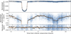 |
Fig. 2 CHEOPS phase-folded phase curve. Data points are shown in blue, and their 10-min binned counterparts are shown in black with error bars. The mean and 3 σ uncertainty of the model are shown in orange (line and shaded area, respectively) and have been computed from a set of 2000 models randomly drawn from the posterior distribution. From top to bottom are show the full phase curve, a zoomed-in version to highlight the phase-curve signal, and the residuals in ppm. |
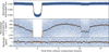 |
Fig. 3 TESS phase-folded phase curve. Data points are shown in blue, and their 10-min binned counterparts are shown in black with error bars. The mean and 3 σ uncertainty of the model are shown in orange (line and shaded area, respectively) and have been computed from a set of 2000 models randomly drawn from the posterior distribution. From top to bottom are show the full phase curve, a zoomed-in version to highlight the phase-curve signal, and the residuals in ppm. |
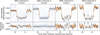 |
Fig. 4 Spitzer phase-folded occultations. Data points are shown in blue, and their 10-min binned counterparts are shown in black with error bars. The mean and 3 σ uncertainty of the model are shown in orange (line and shaded area, respectively) and have been computed from a set of 2000 models randomly drawn from the posterior distribution. The 4 IRAC channels 1, 2, 3, 4, centred at 3.6 μm, 4.5 μm, 5.8 μm, 8.0 μm, respectively, are shown at the top, with their corresponding residuals in ppm at the bottom. |
 |
Fig. 5 Correlation plot of the posterior distribution of the eccentricity e and argument of periastron ω of the orbit of WASP-18 b that match the mid-occultation time |

Values of the eccentricity e and argument of periastron ω.
5.3 Occultation depth variability
We checked for variability of the occultation depth in each instrument passband by fixing all parameters to their best-fit values from our global fit (see Table 3), letting free only the occultation depth (via the dayside flux F max), the noise jitter, σw, and the normalisation flux, f0 . The 3D parameter space was explored with the MCMC algorithm emcee (Foreman-Mackey et al. 2013, 2019).
We fitted each CHEOPS visit individually and extracted the posterior values of  for each epoch. The dayside flux values are represented in Fig. 6. Naturally, the visits not covering any occultation event are poorly constrained, but we obtain a precision of the order of 30 ppm for each of the other ones. We do not detect any strong sign of variability with discrepancies being below 3 σ. To quantify the dayside flux scattering, we calculated the multiplicative factor to be applied to the errorbar to find a distribution consistent with a Normal distribution. For the CHEOPS’ dayside flux, we found a multiplicative factor of 1.05, which is close to 1 and thus showing consistency with Gaussian statistics. We computed the Lomb-Scargle periodogram (Lomb 1976; Scargle 1982) of the series but could not identify any significant periodicity.
We split the TESS sectors into 110 short light curves with a duration of one planetary orbit. Given the TESS cadence, we had about 680 exposures for a full coverage of a planetary orbit, and we discarded 12 out of the 110 data sets that had fewer than 400 points (poor phase-curve coverage). For each of the 98 remaining light curves, we applied the same procedure as for the CHEOPS visits and obtained the  values represented in Fig. 7. The scatter is larger than what is allowed from the uncertainties with 17 data points at >3 σ (all ≲5 σ but 1 at 9.5 σ). The errorbar multiplicative factor is this time of 2.21, further confirming the large inconsistency with Gaussian statistics. We investigated the outliers’ light curves individually and found local variability likely of instrumental origin. No specific periodicity nor dominant timescale could be identified as a significant signal in the Lomb-Scargle periodogram. We note that this variability could also be of stellar origin and induced by supergranulation (e.g. HAT-P-7 b; Lally & Vanderburg 2022).
We selected the Spitzer occultations of the IRAC Channel 2 and fitted them individually similar to what was done for CHEOPS and TESS. The dayside flux values we recover were all consistent with each other (see Fig. 8). The errorbar multiplicative factor is 0.88 for the Spitzer F max values, hence showing clear consistency with Normal distribution statistics. We compared our individual values to the ones published in Deming et al. (2023) and found most of them being consistent (<3 σ) with only 2 out of 11 showing a significant discrepancy (4.1 σ and 3.2σ for AOR keys 53516800 and 53515520, respectively).
The analysis of the occultation depth variability of all three passbands did not reveal any significant signal on the short timescale. Thanks to the very long periods covered by our data sets (3 years for CHEOPS, 5 years for TESS, and 6.7 years for Spitzer), our results demonstrate long-term stability of the dayside of WASP-18 b.
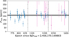 |
Fig. 6 Dayside flux observed in the CHEOPS passband over the three seasons of observations (all three panels). The observations covering an occultation are represented in blue (including a phase curve), and the ones only covering transits in pink. The horizontal black line and shaded areas mark the value |

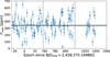 |
Fig. 7 Dayside flux observed in the TESS passband over the 5 sectors: sectors 2 and 3 on the left, sectors 29 and 30 in the center, and sector 69 on the right. The horizontal black line and shaded areas mark the value |

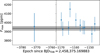 |
Fig. 8 Dayside flux observed in the Spitzer/IRAC/Channel 2 passband for programmes 50517 (left panel) and 11099 (right panel). The horizontal black line and shaded areas mark the value |

6 Atmospheric characterisation
6.1 Planet thermal emission
We discussed in Section 5.1 the upper limits that we obtained on the minimum PC flux values, F
min, from both CHEOPS and TESS passbands. Given that we fixed the phase offset Δφ to 0, F
min actually corresponds to the nightside flux. Assuming a black-body emission for the nightside of WASP-18 b and using synthetic stellar spectra from the PHOENIX library (Husser et al. 2013), we could convert upper limits from flux to temperature. We selected the PHOENIX spectrum with the closest properties to our stellar parameters: T
eff = 6300 K, logg = 4.5 and [Fe/H] = 0.0. We modelled the thermal emission of the planet following relationship:
 (13)
(13)
where R
p
and R★
are the planetary and stellar radii, respectively, S(λ, T
night) and S(λ, T★
) are the flux emission spectra of the planet and the star, respectively, and  is the instrumental passband. We downloaded the CHEOPS passband from the CHEOPS Archive Browser10, and the TESS passband from the TESS Science Support Center11. From
  and
and  , we could derive the nightside black-body temperatures,
  and
and  , for the two instruments, leading to an overall limit of T
night < 1970 K.
, for the two instruments, leading to an overall limit of T
night < 1970 K.
We performed a similar analysis for the dayside emission of WASP-18 b using Eq. (13) and replacing F
night by F
day = F
max, and T
night by the so-called brightness temperature T
b. We used F
max from all passbands but Spitzer/IRAC Channels 3 and 4, as their wavelength coverage goes beyond the limit of 5.5μm of the PHOENIX spectra. We obtained the following brightness temperatures:  ,
,  ,
,  , and
, and  . The uncertainties are expected to be underestimated given the fact that we did not propagate the uncertainties of the stellar properties by using a single PHOENIX spectrum. Also, we might be slightly biasing our results by assuming a black-body emission for the planet. However, these results already show some interesting outcomes as the TESS and Spitzer/IRAC/Channel 1 passband agree on a brightness temperature of 2960 K, whereas CHEOPS and Spitzer/IRAC/Channel 2 would be capturing an excess of flux (converted into a higher temperature here). The excess in the CHEOPS passband might actually indicate the presence of reflected light as we probe visible wavelengths. As for Spitzer/IRAC/Channel 2, the larger occultation depth could be explained by the presence of CO (Brogi et al. 2023; Yan et al. 2023) that have emission lines at 4.5 μm. Using the framework of Cowan & Agol (2011) and following the methodology detailed in Section 6.2 of Deline et al. (2022), we estimated the values of the Bond albedo A
B
and the heat redistribution efficiency ε (more details in Appendix F). As usual and expected for UHJs, we obtained very low values of both AB
and ε implying that the planetary atmosphere absorbs most of the incoming energy and redistributes it inefficiently. The narrowest constraints come from the TESS passbands with A
B
≤ 0.13 and ε ≤ 0.21. Interestingly, the maximum dayside temperature that this analytical approach allows is about 3060 K for the extreme case where AB
= ε = 0. This strengthens the hint for an excess of flux, especially in the passband of Spitzer/IRAC/Channel 2. Given the several assumptions made for this analysis of the dayside emission, we consider the aforementioned results as indicative. In the following Sections 6.2 and 6.3, we analysed the dayside emission of WASP-18 b including the recently published JWST values (Coulombe et al. 2023) to complete our 0.6-to-8.0 μm wavelength coverage of occultation depth measurements (see Fig. 9). We used two different approaches to characterise the planetary atmosphere: General Circulation Modelling (GCM) and atmospheric retrieval.
. The uncertainties are expected to be underestimated given the fact that we did not propagate the uncertainties of the stellar properties by using a single PHOENIX spectrum. Also, we might be slightly biasing our results by assuming a black-body emission for the planet. However, these results already show some interesting outcomes as the TESS and Spitzer/IRAC/Channel 1 passband agree on a brightness temperature of 2960 K, whereas CHEOPS and Spitzer/IRAC/Channel 2 would be capturing an excess of flux (converted into a higher temperature here). The excess in the CHEOPS passband might actually indicate the presence of reflected light as we probe visible wavelengths. As for Spitzer/IRAC/Channel 2, the larger occultation depth could be explained by the presence of CO (Brogi et al. 2023; Yan et al. 2023) that have emission lines at 4.5 μm. Using the framework of Cowan & Agol (2011) and following the methodology detailed in Section 6.2 of Deline et al. (2022), we estimated the values of the Bond albedo A
B
and the heat redistribution efficiency ε (more details in Appendix F). As usual and expected for UHJs, we obtained very low values of both AB
and ε implying that the planetary atmosphere absorbs most of the incoming energy and redistributes it inefficiently. The narrowest constraints come from the TESS passbands with A
B
≤ 0.13 and ε ≤ 0.21. Interestingly, the maximum dayside temperature that this analytical approach allows is about 3060 K for the extreme case where AB
= ε = 0. This strengthens the hint for an excess of flux, especially in the passband of Spitzer/IRAC/Channel 2. Given the several assumptions made for this analysis of the dayside emission, we consider the aforementioned results as indicative. In the following Sections 6.2 and 6.3, we analysed the dayside emission of WASP-18 b including the recently published JWST values (Coulombe et al. 2023) to complete our 0.6-to-8.0 μm wavelength coverage of occultation depth measurements (see Fig. 9). We used two different approaches to characterise the planetary atmosphere: General Circulation Modelling (GCM) and atmospheric retrieval.
6.2 General circulation model
We performed forward modelling of the atmosphere of WASP-18 b with the general circulation model (GCM) ExoRad, using the version with full radiative transfer (expeRT/MITgcm; Carone et al. 2020; Schneider et al. 2022)12. We generated synthetic emission spectra of the planetary dayside using the parameters listed in Table 3 as inputs, and normalised the outcomes with the PHOENIX stellar spectra (Husser et al. 2013) up to 5.5 μm, assuming T eff = 6300 K, and a matching black-body SED at longer wavelengths. To calculate the radiative forcing in the model, we assumed solar metallicity and equilibrium chemistry. We included correlated-k tabulated opacities combined to 11 spectral bins, corresponding to the S1 resolution as specified in Schneider et al. (2022) for the following species: H2O (from ExoMol13; Tennyson et al. 2016, 2020), Na (Allard et al. 2019), K (Allard et al. 2019), CO2, CH4, NH3, CO, H2S, HCN, SiO, PH3 and FeH, as well as H− absorption suitable for an ionised atmosphere.
We generated several GCM simulations to derive dayside spectra. We first tested runs without TiO and VO opacities with strong magnetic drag τfric and no drag. Here, we found that already the inclusion of magnetic drag alone yielded a vast improvement in the data fit. We then included TiO and VO opacities (McKemmish et al. 2016, 2019). TiO and VO produce an upper atmosphere thermal inversion that impacts in particular the dayside emission in the optical as observed with CHEOPS and TESS. We then tested various values for magnetic drag and including TiO/VO (see Table 5). Magnetic drag is treated during the simulation by applying uniform friction to the horizontal wind field (u, v) via:
 (14)
(14)
 (15)
(15)
where u and v are the zonal and meridional wind fields, respectively.
The inclusion of magnetic drag is motivated by the substantial degree of ionisation of the dayside atmosphere resulting in the presence of several ions such as Na+, K+, Ca+, Fe+, Al+ and Ti+ (Helling et al. 2019, 2021). The partially ionised flow induces magnetic coupling that in turn affects the winds as already pointed out by Perna et al. (2010); Rodríguez-Barrera et al. (2015). The necessity to account for the impact of magnetic fields in UHJs such as WASP-18 b has been further confirmed several times (Wardenier et al. 2023; Beltz et al. 2022; Demangeon et al. 2024). Recent JWST observations also support the impact of magnetic drag (e.g. WASP-18 b in Coulombe et al. 2023). Table 5 clearly shows that a combination of drag and TiO/VO is needed and that the fit to the data improves with decreasing τfric = 106, 105, 104 s. Coulombe et al. (2023) found with the GCM SPARC/MITgcm a lower value of τfric = 103 s. These authors tested, however, only two scenarios with weak τfric = 106 s and strong drag τfric = 103 s, respectively. They further did not perform a sensitivity study with the GCM with respect to drag and TiO, as we did in this paper. We thus note that the choice of τfric is currently still open for debate, in particular in the uniform drag assumption as implemented here (Perna et al. 2010; Tan & Komacek 2019; Coulombe et al. 2023; Beltz et al. 2022). We found with expeRT/MITcgm that τfric = 104 s already effectively disrupts superrotation at the dayside and yields agreement with the JWST emission spectrum. We further note that τfric = 104 s is currently the smallest drag time scale that was tested in expeRT/MITcgm. Smaller τfric time scales as well as other implementations of magnetic field coupling are currently under investigation. In any case, only full 3D GCMs can assess the impact of magnetic drag on the climate state that shapes horizontal heat transfer and thus the dayside emission. The resulting strong horizontal temperature gradient over the dayside, Δ T > 1000 K, also ensures that the TiO and VO abundances are not constant across the dayside.
Comparing the outcome with the measured occultation depths from CHEOPS, TESS, JWST and Spitzer reveals agreement when both TiO and VO and magnetic drag are used (see Fig. 9 and Table 5). Magnetic drag reduces circulation efficiency, resulting in a hotter dayside such that, even without TiO and VO, the GCM provides a relatively close match to the data, with a reduced χ2
( ) of 8.514. The agreement with the data is nonetheless further improved when including TiO and VO, even with reduced drag. Our best GCM match to the data is obtained when both TiO/VO and a strong drag are present (
 ). Therefore, both the magnetic drag and the presence of a strong, local gas-phase absorber in the optical like TiO and VO known from cool star atmosphere modelling (e.g. Gustafsson et al. 2008; Van Eck et al. 2017) are needed to match the data from the optical to the IR wavelengths. Models without TiO and VO are not shown for clarity but underpredict the emitted planetary flux. We particularly note that the GCM output qualitatively matches with the atmospheric retrieval models (see Section 6.3), including the flattening of the spectrum between 1 and 2 micron due to H2O dissociation. In cooler planets, this wavelength region is dominated by water bands. We note, however, that while our GCM with TiO/VO and magnetic drag shows an upper atmosphere temperature inversion, it is not sufficiently hot for CO emission. Retrieval models show that temperatures higher than 3500 K are required to trigger CO emission (see Fig. 10).
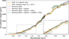 |
Fig. 9 Occultation depths as a function of wavelength. The black points with errorbars represent the measurement from this work (CHEOPS, TESS and Spitzer; 2 leftmost and 4 rightmost points) and from Coulombe et al. (2023) with JWST (0.8-3 μm). The GCM simulations including TiO and VO (Section 6.2) with and without magnetic drag are shown in orange and light brown, respectively. The orange-filled diamonds mark the passband-integrated GCM values with magnetic drag (τfric = 104 s). The retrieval runs (Section 6.3) are shown in blue, pink, purple and green (same colours as in Fig. 10 and Table 6) depending on the data points included in the fit. An inset zoomed-in view of the CHEOPS-to-1.75 μm range is shown in the lower right corner for convenience. |
Goodness-of-fit metrics for the GCM models.
6.3 Atmospheric retrieval
We performed atmospheric-retrieval analyses to characterise the thermal emission properties of WASP-18 b, hence, inferring its thermal and composition structure. We employed the open-source PYRAT BAY package (Cubillos & Blecic 2021) to perform the atmospheric modelling, spectral synthesis, and Bayesian posterior sampling. Since the model only accounts for thermal emission, we primarily constrained the retrievals using the infrared JWST and Spitzer occultations, while running additional fits with and without the optical CHEOPS and TESS occultations to assess how stellar reflected light affected the retrieval results.
The atmospheric model consists of a set of parameterized temperature and composition profiles as a function of pressure (81 layers between 100 and 10−9 bar). We adopted the Madhusudhan & Seager (2009) model to parameterise the temperature profile. The atmosphere of the UHJ WASP-18 b is expected to exceed 2000 K, with the hottest part of the dayside that could reach 3000 K. Since disequilibrium-chemistry processes such as photochemistry and transport-induced quenching become less and less important with increasing effective temperature, at the extreme temperatures seen on WASP-18 b, the chemical reaction rates are fast enough to overcome the effect of disequilibrium chemistry (Kopparapu et al. 2012; Moses 2014; Madhusudhan et al. 2016; Venot et al. 2018). If disequilibrium chemistry occurs at all, it would occur at high altitudes above the pressures probed by the observations presented in this work, and thus the modeled emission spectra of planets such as WASP-18 b would not be significantly impacted (Shulyak et al. 2020)15. Thermochemical equilibrium is therefore a reasonable assumption to model the dayside atmospheric composition of WASP-18 b and its corresponding emission spectra. The chemical network consists of 45 neutral and charged species, accounting for the main H, He, C, O, N, Na, K, S, Si, Fe, Ti, and V-bearing species expected to form in the atmosphere. We defined three retrieval parameters to sample the composition parameter space: the oxygen elemental abundance relative to solar values, [O/H]; the carbon abundance relative to solar values, [C/H]; anda catchall parameter to scale all other metal abundances relative to solar values, [M/H]. Finally, we computed the height of the pressure layers assuming hydrostatic equilibrium. Table 6 lists the retrieval parameters, priors, and posterior values.
For the spectral synthesis, we considered line-sampled opacities from the dominant molecular species from the HITEMP (CH4, CO, and CO2; Rothman et al. 2010) and ExoMol databases (H2O, HCN, NH3, TiO, VO, and C2H2; Tennyson et al. 2016, 2020). Prior to the retrievals, we tabulated the opacity line lists into a cross-section grid of temperatures, pressures, and wavenumbers (at a constant resolving power of R = 20 000). We pre-processed the larger line lists with the repack package to extract the dominant line transitions (Cubillos 2017). Additionally, we considered opacities from the Na and K resonant lines (Burrows et al. 2000), collision-induced absorption for H2-H2 (Borysow et al. 2001; Borysow 2002; Jørgensen et al. 2000) and H2-He (Borysow et al. 1988; Borysow & Frommhold 1989; Borysow et al. 1989), Rayleigh scattering for H, H2, and He (Kurucz 1970), and H− free-free and bound-free (John 1988). We adopted a PHOENIX stellar model as the flux spectrum for WASP-18. We performed the Bayesian posterior sampling using the Nested Sampling algorithm (Skilling 2004, 2006) as implemented in the MultiNest package (Feroz et al. 2009; Buchner et al. 2014), employing 1500 live points.
To assess the impact of each observation in constraining the atmospheric properties, we performed four retrieval analyses considering different sets of observing constraints. First, we performed retrievals using only the JWST occultations. Next, we added the Spitzer occultations to test the role of infrared absorbers. Finally, we included the TESS and CHEOPS occultations to test the impact of optical absorbers and reflected light. As expected, the JWST observations dominate the retrieval results, resulting in a consistent fit to the H2O bands between 1.0 and 2.5 μm. However, we found that retrievals with and without the Spitzer constraints lead to widely different temperature and composition outcomes (see Figs. 10 and 11, and Table 6). The driving factor is the high signal-to-noise IRAC2 occultation depth at 4.5 μm. The much larger brightness temperature at 4.5 μm than that of the JWST occultations requires an atmosphere with significant CO/CO2 absorption (as highlighted by the diagonally hatched area in left panel of Fig. 10), which in turn leads to super-solar carbon and oxygen abundances of 3-5 times solar. We also noted that incorporating the Spitzer occultations to the retrieval constraints results in steeper temperature gradients. This adjustment is expected given the stark brightness-temperature difference between the JWST and the Spitzer 4.5-μm observations (Fig. 10, right panel). In contrast, the retrieval of the JWST data alone returns an atmosphere with solar-to-subsolar abundances, well in agreement with the previous analysis by Coulombe et al. (2023).
Finally, we compared the retrieved thermal-emission spectra with the measurements in the CHEOPS and TESS passbands to look for the presence of reflected light coming from the planet. The left panel in Fig. 10 displays the retrieval models integrated over all instrumental passbands as coloured diamonds. Table 7 lists the thermal flux values retrieved for each one of the four retrieval models. We detail below the comparison within the CHEOPS and TESS passbands in the cases for which the Spitzer data were included in the retrieval fit (pink, purple and green). First, when only JWST and Spitzer data points were included in the retrieval fit (pink model), we found that the measured occultation depth in the TESS passband was significantly below the retrieval value (at 4.1 σ). Therefore, the inclusion of the TESS data point in the retrieval runs is necessary to properly model the data by mitigating the amount of thermal emission in the TESS passband. With the TESS data point included, we compared two retrieval runs with and without fitting the CHEOPS data point (green and purple models, respectively). When discarding CHEOPS from the fit, the retrieval model showed a smaller flux difference in the TESS passband (−11.1 ± 8.2 ppm). If we convert the flux difference into a 3-σ upper limit on the reflected light in the TESS passband, we get  ppm, which corresponds to a geometric albedo16 of
  .
.
The passband-integrated value of this model for CHEOPS gives a thermal flux of  ppm, which is smaller than the measured dayside flux by 2.6 σ. Explaining this difference with reflected light means
  ppm and a corresponding geometric albedo of
  . In our last run, we included all data points in the fit (green model) and analysed the effect on the limits of reflected light in both TESS and CHEOPS passbands. As listed in Table 7, we obtained a larger flux difference for TESS and smaller for CHEOPS, at −2.2 σ and +2.0 σ, respectively. These correspond to limits on geometric albedos of
  and
and  .
.
Our retrievals indicate that a significant fraction of the short-wavelength thermal emission originates from TiO/VO (Figure 10, right panel). Although the high planetary mass of WASP-18 b can potentially enhance the efficiency of cold-trapping - hence depleting heavier metals from the atmosphere (Beatty et al. 2017) -, our retrieved thermal profiles lie well above the thermal stability curves for Ti-bearing and other refractory species. This suggests that the dayside of WASP-18 b remains sufficiently hot to inhibit vertical cold-trapping (Spiegel et al. 2009), and thus allow for the presence of heavy metals like TiO, VO, and alkali metals in gas form in its atmosphere. While day-night cold-trapping remains a plausible scenario, additional phase-curve observations of the nightside emission are needed to evaluate its potential (Parmentier et al. 2013). However, Beatty et al. (2017) argued that observations of planets with daysides of 3000 K and hotter like this planet appear to escape nightside trapping. Figure 10 also elucidates why this would be the case. The dayside is too hot for TiO thermal stability even down to 100 bar. For such a high gravity and fast rotating planet, superrotation is expected to extend well down to 100 bar and deeper into the planet (Carone et al. 2020). Thus, an efficient horizontal heat and material transport is expected below 10 bar. Even if TiO would condense out (i.e. be thermally stable) on the nightside, it would evaporate again at depth and be transported towards the dayside, where it could again dominate the gas absorption in the optical wavelength range in agreement with the results in this work. This is also in line with the study of Helling et al. (2019), where they infer the absence of clouds on the dayside of WASP-18 b from cloud formation models.
We conclude that both the scenario including TESS only and the scenario including CHEOPS+TESS strongly constrain the amount of reflected light in the TESS passbands to extremely low values (< 0.017). This is not unexpected as many atmospheres of UHJs have been reported to be very dark (e.g. Wong et al. 2021). In the shorter wavelength CHEOPS band, we find tentative (2.6 σ) evidence for reflected light, indicative of stronger atmospheric scattering than in the TESS passband. Even so, it’s amplitude remains low, constrained to a geometric albedo below 0.059. The overall reflectivity remains nonetheless very low as well for CHEOPS, in line with expectations for UHJs. As the geometric albedo is wavelength-dependent, the difference in passbands between CHEOPS and TESS prevents us from performing a quantitative comparison between the two instruments. Fig. 12 shows how the reflected light detection of WASP-18 b computed in this work aligns well with previously published  values for other hot exoplanets (Lendl et al. 2020; Hooton et al. 2022; Deline et al. 2022; Brandeker et al. 2022; Scandariato et al. 2022; Parviainen et al. 2022; Demory et al. 2023; Krenn et al. 2023; Pagano et al. 2024; Singh et al. 2024; Demangeon et al. 2024; Akinsanmi et al. 2024; Scandariato et al. 2024). We also included measurements from the Kepler instrument (Koch et al. 1998; Borucki et al. 2010) as its passband probes essentially the same wavelength range as CHEOPS (Deline et al. 2020). Geometric albedos values in the Kepler passband have been reported in several publications (Esteves et al. 2015; Angerhausen et al. 2015; Heng et al. 2021; Morris et al. 2024). We selected values from the works of Esteves et al. (2015) and Morris et al. (2024) as they performed self-consistent analysis accounting for the contribution of thermal emission in the planetary dayside flux17.
From our analysis, we derived a strong upper limit on the contribution of the reflected light of WASP-18 b in the TESS passband. Despite its significant overlap with the CHEOPS passband (Deline et al. 2020), the latter has a much less stringent constraint with a hint of detection in CHEOPS at 2.6 σ. We explored the scattering properties of the atmosphere that could produce reflected light signals consistent with our computed geometric albedo values in both passbands. Since the dayside of WASP-18 b is likely too hot for condensates to be formed, the only reflective component of the atmosphere would be Rayleigh scattering by molecular and atomic hydrogen as well as helium. We estimated the geometric albedo of the dayside based on the retrieval results shown on the left-hand side of Fig. 11 and the corresponding median temperature profile depicted in Fig. 10. Given the temperature profile and the stated element abundances, we calculated the chemical composition (assuming chemical equilibrium) and the atmospheric absorption coefficients for the chemical species described above and Rayleigh scattering contributions by atomic and molecular hydrogen as well as helium. For the pressure, we chose 0.1 bar, which is the region where the contribution function peak, as shown in Fig. 10. Based on the computed absorption and scattering coefficients we then obtained the wavelength-dependent geometric albedo A g following the analytic solution derived by Heng et al. (2021). The corresponding stellar and planet fluxes were then finally integrated over the CHEOPS and TESS passbands to estimate the A g-contribution of the corresponding measurements.
The wavelength-dependent albedo and the passbands are shown in Fig. 13. The atmospheric species that decisively affects the visible wavelength region for a hot planet such as WASP-18 b is the hydrogen anion H−. Its very strong continuum absorption tends to produce black-body like spectra with only very little contributions by scattering (see Kitzmann et al. 2018, for example). As the yellow curve in Fig. 13 suggests, the geometric albedo of WASP-18 b would be quite low. The albedo still increases towards lower wavelengths due to the λ−4-dependence of Rayleigh scattering, such that the contributions by scattering are higher at the blue end of the CHEOPS passband than in the one of TESS. However, with a passband-integrated geometric albedo for CHEOPS of 0.0013, the estimated value remained below the retrieved value of  .
.
Since the most important species affecting the shortwave albedo is H− (see Fig. H.2), we performed two additional calculations that are depicted in Fig. 13. In the first we artificially removed H− (blue line). This leads to a strong increase in the geometric albedo, producing a CHEOPS Ag value of 0.09, while the corresponding value for TESS would be 0.017. In the second additional calculation, the chemical-equilibrium abundance of H− was reduced by 98% (orange curve), which yields  and
and  , more comparable to the retrieval results.
Besides H−, other short-wave absorbers, such as TiO and VO or the alkali metals Na and K can also impact the amount of scattered light and, thus, the geometric albedo. For the case of no H− absorption, we also show the resulting geometric albedos when removing these species as opacity sources in Fig. H.2. As the results suggest, the impact of TiO and VO on the geometric albedo is negligible for the atmosphere of WASP-18 b. The alkali metals, however, clearly have a stronger impact. When removing them, in addition to H−, we obtain the analytical limit of 0.75 for the geometric albedo in case of Rayleigh scattering.
However, the impact of these species can only be noticed when H− is not present. In Fig. H.1 of Appendix H we show the impact of the additional shortwave absorbers on Ag as a function of H−. These results suggest that as long H− is not removed entirely, the effect of all of these additional species on the geometric albedo is minimal.
A H− abundance lower than the one expected from chemical equilibrium can clearly be caused by non-equilibrium effects, including, for example, photochemistry. Furthermore, our estimated value of Ag is based on a one-dimensional description. In the real three-dimensional atmosphere, the abundance of H− should be expected to change considerably across the visible dayside since its abundance is very strongly temperature-dependent.
WASP-18 b retrieval analyses.
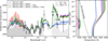 |
Fig. 10 Brightness-temperature spectra derived from the atmospheric retrieval analyses. The circle markers with error bars show the observed occultation depths with uncertainties. The two leftmost circles (red) correspond to CHEOPS and TESS passbands, while the four rightmost black points cover the Spitzer/IRAC channels. The JWST spectroscopic observations are shown in black between 0.8 and 3.0 μm and have been binned down for better visualisation. The coloured solid curves with shaded areas denote the retrieved median spectra and span of the 1σ credible interval for the four model fits (see legend). The diamond markers show the model spectra integrated over the photometric bands. The grey shaded areas highlight the contributions of some relevant species to thermal emission: alkali/H− and TiO/VO in the blue end, and CO/CO2 in the infrared. Right panel: the median (solid curves) and 1σ credible interval (shaded area) of the temperature-profile posterior distributions (same colour coding as in the left panel). The curves on the left edge show the normalized contribution functions that indicate the pressures mainly probed by the observations according to each retrieval analysis. The dashed black line shows the thermal stability curve for TiO2. Other thermal stability curves for species of interest, such as alkali metals (Na2S or KCl), are situated at even lower temperatures around ~1000 K. |
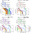 |
Fig. 11 Atmospheric retrieval compositions (each quadrant shows one of the four retrieval runs, labelled in bold text). Top: pairwise and marginal posterior distributions for the abundance free parameters. The quoted values on top of the marginal histograms denote the median and 1σ credible interval for each parameter (span of the central 68% percentiles, also denoted as the shaded areas). The black diagonal dashed lines denote the parameter space values where both parameter are scaled by the same amount (relative to solar abundances). Bottom: volume mixing ratios (VMR) for each retrieval corresponding to the posterior distributions shown above. The shaded areas denote the 1σ credible-interval span in VMR for selected species (see labels at the right of the bottom right quadrant). The solid curves on the left edge of the VMR panels show the contribution functions that indicate the pressures probed by the observations. |
Retrieved thermal flux in the CHEOPS and TESS passbands.
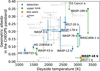 |
Fig. 12 Geometric albedo of several hot and ultra-hot exoplanets as function of their estimated dayside temperature. The detection values (blue) or upper limits (green) are measured in the CHEOPS passband ( |

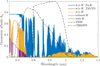 |
Fig. 13 Estimated geometric albedo of WASP-18 b based on the retrieval results in comparison to the passbands of CHEOPS and TESS. The green line shows the geometric albedo with an H− abundance derived by assuming chemical equilibrium (extremely low Ag values, reaching 0.03 at short wavelengths). For the purple line, this abundance is artificially reduced by 98% (yielding Ag values comparable to our results in the CHEOPS and TESS passbands), while for the yellow case the H− continuum is entirely removed as an opacity source. We further explored the effect of removing TiO and VO (red) as well as Na and K (blue). The impact of the former is negligible and the red curve lies hidden behind the yellow model. The latter reveals however more significant scattering spectral features, especially in the CHEOPS and TESS passbands. The strong increase of Ag towards lower wavelengths is caused by the λ−4-dependence of Rayleigh scattering. |
7 Conclusion
We performed a joint analysis of the phase-curve and occultation observations of the planet WASP-18 b, covering six passbands from the visible to the mid-infrared with the space-based instruments CHEOPS, TESS, and the four IRAC channels of Spitzer. We included several signals related to the planet in our modelling; namely, the transit, the occultation, the phase signal, the ellipsoidal variations, the Doppler boosting, and the light travel time. We derived new ephemerides with precisions of 1 second and 1.4 millisecond for the time of inferior conjunction and the orbital period, respectively. We measured a planetary radius of Rp = 1.1926 ± 0.0077 RJ , reaching a precision of 0.65% (equivalent to 550 km).
We interpreted a timing inconsistency with the time of superior conjunction from the JWST observation (Coulombe et al. 2023) as a consequence of the slight orbital eccentricity of the planet. Using priors on the eccentricity and the argument of periastron from radial-velocity measurements (Triaud et al. 2010; Nymeyer et al. 2011; Csizmadia et al. 2019), we substantially improved the constraints on the argument of periastron with a value of  for an eccentricity of e = 0.00852 ± 0.00091. Despite the relative youthfulness of the WASP-18 system, having such a short-period massive planet on an eccentric orbit is peculiar and might require further study to understand the formation and stability of the planetary orbit.
We investigated the occultation depth values across the 15 years covered by our data sets and we were not able to detect either short-term nor long-term variability.
From the upper limits on the nightside flux in the CHEOPS and TESS passbands, we derived a maximum nightside temperature estimate of T night < 2000 K. Modelling the dayside emission with general circulation models (GCMs) showed that the presence of magnetic-driven friction and super-solar metallicity are necessary to explain our observations. We also fit the occultation depths, including the data from JWST (Coulombe et al. 2023), with an atmospheric retrieval model. We were able to show that new Spitzer data at 4.5 μm reveal super-solar carbon and oxygen abundances, with significant CO/CO2 absorption, and a steep inverted temperature gradient throughout the planetary atmosphere. Overall, we found that the retrievals provided a good fit to the observations. However, the difference in brightness temperature inferred from the CHEOPS and TESS occultation depths was not captured by any of the models. This could be indicative of missing physics in the retrievals, such as the omission of reflected stellar light or atmospheric variations across latitude and longitude. We note that while GCMs do help in investigating the 3D effects of the physics, they are not strict fits to the data. Ultimately, future phase-curve or dayside-mapping observations will be critical to better constrain the spatial variation of the physical properties of WASP-18 b, allowing us to fine-tune our GCMs and construct more sophisticated retrieval models.
Finally, we explored the potential contribution of reflected light to the dayside brightness in the CHEOPS and TESS passbands. We strongly constrained the geometric albedo in TESS with a 3-σ upper limit of  . In parallel, the CHEOPS passband showed a hint of flux excess at 2.6σ that corresponds to a geometric albedo
  . This result suggests the presence of a very weak reflectivity of the planetary atmosphere. We modelled the scattering properties of WASP-18 b to match our derived Ag
values. We quantitatively reproduced this behaviour as the result of Rayleigh scattering in the presence of continuum absorption by H−. The abundance of H− needs to deviate from chemical equilibrium to match the geometric albedo in the CHEOPS and TESS passbands, which can be caused by non-equilibrium effects (e.g. photochemistry) or significant temperature variations across the planetary dayside.
. This result suggests the presence of a very weak reflectivity of the planetary atmosphere. We modelled the scattering properties of WASP-18 b to match our derived Ag
values. We quantitatively reproduced this behaviour as the result of Rayleigh scattering in the presence of continuum absorption by H−. The abundance of H− needs to deviate from chemical equilibrium to match the geometric albedo in the CHEOPS and TESS passbands, which can be caused by non-equilibrium effects (e.g. photochemistry) or significant temperature variations across the planetary dayside.
Data availability
Raw and detrended light curves are available at the CDS via anonymous ftp to cdsarc.cds.unistra.fr (130.79.128.5 or via https://cdsarc.cds.unistra.fr/viz-bin/cat/J/A+A/699/A150
Appendix A CHEOPS observations
List of the CHEOPS observations.
 |
Fig. A.1 CHEOPS raw light curves. The 37 CHEOPS visits are displayed in coloured data points from top to bottom with their corresponding models shown as black lines. The planet model at the top (continuous black line) is the final model with only astrophysical signals (see Eq. 12). |
Appendix B TESS observations
List of the times in BJDTDB used to discard TESS data points.
 |
Fig. B.1 TESS raw light curves extracted by the SPOC. The coloured points, blue and green, represent the photometric data of the two orbits of each sector. The black points are the data binned at a cadence of 30 min. The shaded areas highlight the photometric ranges that were discarded due to the presence of remaining systematic trends. The times in BJDTDB of the different cuts are listed chronologically in Table B.1. The light curve of sector 3 corresponds to the SAP flux (second panel) and the other sectors (2, 29, 30 and 69) are all PDCSAP fluxes. |
Appendix C Spitzer observations
List of the Spitzer observations.
Appendix D Phase-curve model
We provide details about the expression of the phase-curve model used in this work and reported in Eq 3.
We start by defining the phase-curve signal of the planet as a function of the planetary phase angle α:
 (D.1)
(D.1)
where a
PC
and b
PC
are the phase-curve semi-amplitude and a constant offset, respectively. We defined those two parameters in such a way that the phase-curve signal F
p reaches a maximum Fmax when α = 0 deg and a minimum F
min
when α = 180 deg, which corresponds to rewriting the previous equation as follows:
 (D.2)
(D.2)
We then used the expression of the phase angle α as a function of the angular position of the planet θ and the orbital inclination i:
 (D.3)
(D.3)
Here we have defined θ in such a way that the inferior conjunction occurs at θ = 90 deg. We note that when the planetary orbit is not viewed edge-on (i.e. i ≠ 90 deg), one has 0deg < α < 180 deg and the phase-curve signal F p never reaches the values F min and F max.
The angular position of the planet can be written θ = ω + ν, with ω and ν being the argument of periastron and the true anomaly, respectively. In order to account for potential phase shift between the superior conjunction (θ = 270 deg) and the phase-curve maximum value (e.g. due to a hotspot offset), we introduce the term Δφ in our expression of θ:
 (D.4)
(D.4)
We chose to subtract the phase shift value, Δφ, to ensure that a positive Δφ induces a positive time delay, which means that the phase-curve maximum will occur after the superior conjunction (e.g. westward hotspot offset).
We obtain the phase-curve model reported in Eq. 3 by merging Eqs. D.4 and D.3 into Eq. D.2.
Appendix E Ellipsoidal variations model
The ellipsoidal variations correspond to the photometric variability created by the rotation of a distorted star, which deformation is caused by the tidal forces of a close-by massive planet.
In the work of Kopal (1959), the light variation due to stellar distortion is derived in Section IV.2 of chapter IV as a series function of tesseral harmonics. considering the tidal lag negligible, the tesseral harmonics reduce to Legendre polynomials and the light variation can be simplified (Eq. IV-2-37 of Kopal 1959) as shown below up to the third harmonic:
![Mathematical equation: \begin{aligned} \delta\mathfrak{L} =\ &X_2^{(k)}\left(1+\frac{\beta_2}{4}\right)\left[\frac{v_1^{(2)}}{3}P_2\!\left(n_0\right)-w_1^{(2)}P_2\!\left(l_0\right)\right]\\ &- X_3^{(k)}\left(1+\frac{\beta_3}{10}\right)w_1^{(3)}P_3\!\left(l_0\right)\\ &+ \dots, \end{aligned}](/articles/aa/full_html/2025/07/aa50939-24/aa50939-24-eq170.png) (E.1)
(E.1)
where:
-
 are functions of the limb-darkening coefficients (k = 2 for the linear law, k = 3 for the quadratic law) detailed in Eqs. IV-2-38 and IV-2-39 of Kopal (1959),
 -
β j = [1 + η j (R★ )] y from Eq. IV-2-31 of Kopal (1959), where
![Mathematical equation: $\eta_j\!\left(R_\star\right)\in\left[j-2; j+1\right]$](/articles/aa/full_html/2025/07/aa50939-24/aa50939-24-eq172.png) depends on the density distribution within the star (Eqs. II-2-5 and II-2-6 of Kopal 1959 with a
1 ≡ R★
), and y is the gravity-darkening coefficient,
depends on the density distribution within the star (Eqs. II-2-5 and II-2-6 of Kopal 1959 with a
1 ≡ R★
), and y is the gravity-darkening coefficient, -
Pn (x) is the n th Legendre polynomials, i.e.
 and
and  ,
, -
n 0 = cos(i) and l 0 = cos(ψ) sin(i), where i is the orbital inclination (from the plane of the sky) and ψ is the true anomaly reckoned from the moment of inferior conjunction18, i.e. ψ = ω + ν - π/2 and l 0 = sin(ω + ν) sin(i ),
-
 refers to the rotational distortion and will therefore be ignored (this term is time-independent),
 -
 refers to the tidal distortion, i.e. ellipsoidal variations, and
  from Eqs. IV-2-33 and IV-2-56 of Kopal (1959) (with
  , and
, and  ) where
  (Eq. II-1-27 of Kopal 1959).
The two limits reported on η
j
(R★
) depend on the density distribution within the star (Eqs. II-2-4 to II-2-8 of Kopal 1959). The lower limit j - 2 assumes a constant density distribution throughout the stellar interior. The upper limit j + 1 represents the case where all the mass is concentrated at the center of the star. We follow Morris (1985) and thus Esteves et al. (2013), assuming the latter case to simplify the equations and obtain  and
and  .
.
When discarding the rotational distortion ( ) and assuming a point-mass stellar density distribution (η
j
(R★
) = j + 1), we can rewrite Eq. E.1, describing the light variation due to stellar distortion, as follows:
) and assuming a point-mass stellar density distribution (η
j
(R★
) = j + 1), we can rewrite Eq. E.1, describing the light variation due to stellar distortion, as follows:
![Mathematical equation: \begin{aligned} \delta\mathfrak{L} =\ &X_2^{(k)}\left(1+y\right) \frac{M_p}{M_\star}\left[\frac{R_\star}{r\!\left(\theta\right)}\right]^{3} \frac{1-3\sin^2\!\left(\theta\right)\sin^2\!\left(i\right)}{2}\\ &X_3^{(k)}\left(1+\frac{y}{2}\right) \frac{M_p}{M_\star}\left[\frac{R_\star}{r\!\left(\theta\right)}\right]^{4} \frac{3\sin\!\left(\theta\right)\sin\!\left(i\right)-5\sin^3\!\left(\theta\right)\sin^3\!\left(i\right)}{2}\\ &+ \dots \end{aligned}](/articles/aa/full_html/2025/07/aa50939-24/aa50939-24-eq184.png) (E.2)
(E.2)
Here,  and θ = ω + ν = ψ + π/2.
We can further simplify the expression of the light variation in the case of a circular orbit (e = 0) where one has r(θ) = a. By discarding all but the time-dependent terms (i.e. the terms depending on θ), we can obtain from Eq. E.2 the following expression of  :
:
![Mathematical equation: \begin{aligned} \delta\mathfrak{L} = \frac{M_p}{M_\star}\left(\frac{R_\star}{a}\right)^{\!3} \Bigg[ &\frac{3}{4} X_2^{(k)} \left(1+y\right) \sin^2\!\left(i\right) \cos\!\left(2\theta\right)\\ &+ \frac{3}{4} X_3^{(k)}\left(2+y\right) \frac{R_\star}{a} \left(1-\frac{5}{4}\sin^2\!\left(i\right)\right) \sin\!\left(i\right) \sin\!\left(\theta\right)\\ &+ \frac{5}{16} X_3^{(k)}\left(2+y\right) \frac{R_\star}{a} \sin^3\!\left(i\right) \sin\!\left(3\theta\right)\\ &+ \dots \Bigg] \end{aligned}](/articles/aa/full_html/2025/07/aa50939-24/aa50939-24-eq187.png) (E.3)
(E.3)
This expression is the one reported in Eqs. 1–3 of Morris (1985) where the higher order terms (represented by the dots) have been neglected19.
We can finally write the expression of the light variation of Eq. E.3 in a more compact way:
![Mathematical equation: \delta\mathfrak{L} = A_\text{EV}\,\left[\cos\!\left(2\theta\right) - A_1\sin\!\left(\theta\right) + A_3\sin\!\left(3\theta\right) + \dots\right],](/articles/aa/full_html/2025/07/aa50939-24/aa50939-24-eq188.png) (E.4)
(E.4)
where
 (E.5)
(E.5)
 (E.6)
(E.6)
 (E.7)
(E.7)
Here, we retrieve the expressions of the Eqs. 5, 6, 7 and 8 of Section 4.2.3.
Based on the Eqs. IV-2-15 and IV-2-39 of Kopal (1959), we can write the functions of the limb-darkening coefficients  for the quadratic limb-darkening law, i.e. for k = 3. For this, we also need to take into account that quadratic LD law used in Kopal (1959) is different from the commonly used law reported in Manduca et al. (1977) and implemented in the Python code batman (Kreidberg 2015). Indeed, the LD law from Manduca et al. (1977) is
  , whereas the one from Kopal (1959) is
  . By applying the transformations
  and υ2 = -υ
2 = in Eqs. IV-2-15 and IV-2-39 of Kopal (1959), we obtain:
and υ2 = -υ
2 = in Eqs. IV-2-15 and IV-2-39 of Kopal (1959), we obtain:
 (E.8)
(E.8)
 (E.9)
(E.9)
from which the expressions of αEV and βEV of Section 4.2.3 are derived (see Eqs. 9 and 10). Note that when u 2 = υ2 = 0, we get the expression for the linear limb-darkening law reported in Morris (1985) and Esteves et al. (2013).
Appendix F Bond albedo and heat redistribution efficiency
Here, we briefly explain an analytical method detailed in Deline et al. (2022) to estimate the Bond albedo AB and the heat redistribution ε.
We define the average effective temperature of a planet  by:
by:
 (F.1)
(F.1)
where T p is the local effective temperature in the planet atmosphere and dΩ describes a surface element of the atmosphere.
Assuming the planet is emitting as a black body at thermal equilibrium (i.e. absorbed flux equals emitted flux), we can write the following relationship with the average effective temperature of the planet:
 (F.2)
(F.2)
where A
B
is the Bond albedo, σSB is the Stefan-Boltzmann constant, R★
is the stellar radius, a is the semi-major axis, and S(λ, T★
) is the flux emission spectrum of the star as a function of its temperature,  , and the wavelength, λ.
The parametrisation of Cowan & Agol (2011) allows one to estimate the dayside and nightside effective temperatures as functions of the heat redistribution efficiency ε and  :
:
 (F.3)
(F.3)
 (F.4)
(F.4)
Therefore, from these equations, we can compute a relationship between A
B
and ε for a given dayside or nightside temperature, and constrain the range of possible values for these two parameters. Usually, the measured and constrained value is the dayside temperature, T
day, from the occultation depth, and we derive the range of values  . In the framework of Cowan & Agol (2011), the maximum dayside temperature is reached when A
B
= ε = 0, and one obtains
. In the framework of Cowan & Agol (2011), the maximum dayside temperature is reached when A
B
= ε = 0, and one obtains
 (F.5)
(F.5)
Appendix G Detailed Exorad description
The Exorad GCM used the MITgcm dynamical core to solve the hydrostatic primitive equations (e.g. Showman et al. 2009) on a rotating sphere in an Arakawa C-type cubed-sphere grid that spans in the horizontal plane 128 x 64 cells in longitude and latitude, respectively. In vertical direction it follows the formalism established in Carone et al. (2020): in the vertical direction, 41 logarithmically spaced grid cells between 10−5 bar and 100 bar are combined with six linearly spaced grid cells between 100 bar and 700 bar, resulting in 47 vertical cells.
Following Showman et al. (2009), a fourth-order Shapiro filter with dampening time scale τ
shap
= 25 s is used to remove small grid scale noise after each time step from the horizontal velocity fields20. The GCM is stabilised against non-physical gravity wave reflection on top of the modelling domain by implementing a sponge layer between 10−4 and 10−5. The zonal horizontal velocity u is damped by a Rayleigh friction term towards its longitudinally averaged mean ū via:
 (G.1)
(G.1)
where t is the time and k is the strength of the Rayleigh friction applied within the sponge layer, depending on pressure p by:
![Mathematical equation: k = k_{\rm top} \cdot \rm max \left[0,1- \left(\frac{p}{p_{\rm sponge}}\right)^2 \right]^{2}](/articles/aa/full_html/2025/07/aa50939-24/aa50939-24-eq208.png) (G.2)
(G.2)
The control parameters p sponge and k top determine the position and strength of the applied Rayleigh friction in the sponge layer. In this paper, the default values k top = 20 days−1 and 4 sponge = 10−4 bar are used.
To stabilise the deep layers, basal drag is applied to the zonal u and meridional wind velocity v in pressure layers deeper than 400 bar via:
 (G.3)
(G.3)
 (G.4)
(G.4)
where the control parameter k
deep is defined as
![Mathematical equation: k_{\rm deep} = k_{\rm bottom} \cdot \rm max \left[0, \frac{p-490\,\rm bar}{700\,\rm bar - 490\,\rm bar} \right]](/articles/aa/full_html/2025/07/aa50939-24/aa50939-24-eq211.png) (G.5)
(G.5)
with k bottom = 1 day−1.
The model was run with a dynamical timestep Δ t = 25 s for 1000 days simulation time to ensure that the temperature structure does not evolve anymore in the modelling domain· Fluxes are recalculated every fourth dynamical timestep.
Performance tests for the sponge layer and basal drag can be found in Carone et al. (2020). Full radiative transfer was established with the expeRT/MITgcm-branch of the ExoRad framework. A more detailed description of the radiative transfer implementation and performance tests can be found in Schneider et al. (2022).
Appendix H Additional geometric albedo calculations
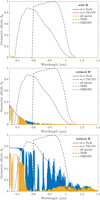 |
Fig. H.1 Estimated geometric albedo of WASP-18 b based on the retrieval results in comparison to the passbands of CHEOPS and TESS. The top panel shows the geometric albedo with the H− abundance derived by assuming chemical equilibrium and for several species removed as opacity source (note that all curves overlap as H− dominates and other opacity sources are negligible). In the middle panel, H− abundance is artificially reduced by 98%, for which A g values are comparable to our results in the CHEOPS and TESS passbands (i.e. the red and yellow curves overlap, but the effect of removing Na and K starts to appear around 600 nm). In the lower panel, the H− continuum is entirely removed, and the removal of alkali (Na and K) reveals even more strongly the scattering features, while the effect of TiO and VO remains negligible (overlap of red and yellow models). The strong increase of A g towards lower wavelengths is caused by the λ−4-dependence of Rayleigh scattering. In the last case, when Na and K are removed as well, the geometric albedo converges towards its analytical limit of 0.75 for Rayleigh scattering. |
 |
Fig. H.2 Estimated geometric albedo of WASP-18 b as a function of the abundance of H−. The A g values are computed based on the retrieval results in comparison to the passbands of CHEOPS and TESS. The H− abundance that best matches our measurements reported in Section 6.3 lies around 2% of the expected chemical equilibrium value (100% on the x-axis), i.e. a reduction of 98%. |
Appendix I Joint-fit values of the systematic parameters
Values of the systematic parameters for CHEOPS.
Values of the systematic parameters for TESS.
Values of the systematic parameters for Spitzer.
Appendix J Acknowledgements
This project has received funding from the European Research Council (ERC) under the European Union’s Horizon 2020 research and innovation programme (project FOUR ACES, grant agreement No. 724427). It has also been carried out in the frame of the National Centre for Competence in Research “PlanetS” supported by the Swiss National Science Foundation (SNSF). A.De. acknowledges the financial support of the SNSF.
P.E.C. is funded by the Austrian Science Fund (FWF) Erwin Schroedinger Fellowship, program J4595-N.
LCa and CHe acknowledge financial support from the Österreichische Akademie 1158 der Wissenschaften and from the European Union H2020-MSCA-ITN-2019 1159 under Grant Agreement no. 860470 (CHAMELEON). Calculations were performed using supercomputer resources provided by the Vienna Scientific Cluster (VSC).
B.-O. D. acknowledges support from the Swiss State Secretariat for Education, Research and Innovation (SERI) under contract number MB22.00046.
ML acknowledges support of the Swiss National Science Foundation under grant number PCEFP2_194576.
ABr was supported by the SNSA.
MNG is the ESA CHEOPS Project Scientist and Mission Representative, and as such also responsible for the Guest Observers (GO) Programme. MNG does not relay proprietary information between the GO and Guaranteed Time Observation (GTO) Programmes, and does not decide on the definition and target selection of the GTO Programme.
S.C.C.B. acknowledges support from FCT through FCT contracts nr. IF/01312/2014/CP1215/CT0004.
GBr, VSi, LBo, VNa, IPa, GPi, RRa, and GSc acknowledge support from CHEOPS ASI-INAF agreement n. 2019-29-HH.0.
The Belgian participation to CHEOPS has been supported by the Belgian Federal Science Policy Office (BELSPO) in the framework of the PRODEX Program, and by the University of Liège through an ARC grant for Concerted Research Actions financed by the Wallonia-Brussels Federation.
S.G.S. acknowledge support from FCT through FCT contract nr. CEECIND/00826/2018 and POPH/FSE (EC).
The Portuguese team thanks the Portuguese Space Agency for the provision of financial support in the framework of the PRODEX Programme of the European Space Agency (ESA) under contract number 4000142255.
TWi acknowledges support from the UKSA and the University of Warwick.
This project has received funding from the Swiss National Science Foundation for project 200021_200726. It has also been carried out within the framework of the National Centre of Competence in Research PlanetS supported by the Swiss National Science Foundation under grant 51NF40_205606. The authors acknowledge the financial support of the SNSF.
YAl acknowledges support from the Swiss National Science Foundation (SNSF) under grant 200020_192038.
We acknowledge financial support from the Agencia Estatal de Investigación of the Ministerio de Ciencia e Innovación MCIN/AEI/10.13039/501100011033 and the ERDF “A way of making Europe” through projects PID2019-107061GB-C61, PID2019-107061GB-C66, PID2021-125627OB-C31, and PID2021-125627OB-C32, from the Centre of Excellence “Severo Ochoa” award to the Instituto de Astrofísica de Canarias (CEX2019-000920-S), from the Centre of Excellence “María de Maeztu” award to the Institut de Ciències de l’Espai (CEX2020-001058-M), and from the Generalitat de Catalunya/CERCA programme.
DBa, EPa, and IRi acknowledge financial support from the Agencia Estatal de Investigación of the Ministerio de Ciencia e Innovación MCIN/AEI/10.13039/501100011033 and the ERDF “A way of making Europe” through projects PID2019-107061GB-C61, PID2019-107061GB-C66, PID2021-125627OB-C31, and PID2021-125627OB-C32, from the Centre of Excellence “Severo Ochoa” award to the Instituto de Astrofísica de Canarias (CEX2019-000920-S), from the Centre of Excellence “María de Maeztu” award to the Institut de Ciències de l’Espai (CEX2020-001058-M), and from the Generalitat de Catalunya/CERCA programme.
CBr and ASi acknowledge support from the Swiss Space Office through the ESA PRODEX program.
ACC acknowledges support from STFC consolidated grant number ST/V000861/1, and UKSA grant number ST/X002217/1.
ACMC acknowledges support from the FCT, Portugal, through the CFisUC projects UIDB/04564/2020 and UIDP/04564/2020, with DOI identifiers 10.54499/UIDB/04564/2020 and 10.54499/UIDP/04564/2020, respectively.
This project was supported by the CNES.
The Belgian participation to CHEOPS has been supported by the Belgian Federal Science Policy Office (BELSPO) in the framework of the PRODEX Program, and by the University of Liège through an ARC grant for Concerted Research Actions financed by the Wallonia-Brussels Federation.
L.D. thanks the Belgian Federal Science Policy Office (BELSPO) for the provision of financial support in the framework of the PRODEX Programme of the European Space Agency (ESA) under contract number 4000142531.
This work was supported by FCT - Fundaçâo para a Ciência e a Tecnologia through national funds and by FEDER through COMPETE2020 through the research grants UIDB/04434/2020, UIDP/04434/2020, 2022.06962.PTDC.
O.D.S.D. is supported in the form of work contract (DL 57/2016/CP1364/CT0004) funded by national funds through FCT.
MF and CMP gratefully acknowledge the support of the Swedish National Space Agency (DNR 65/19, 174/18).
DG gratefully acknowledges financial support from the CRT foundation under Grant No. 2018.2323 “Gaseousor rocky? Unveiling the nature of small worlds”.
M.G. is an F.R.S.-FNRS Senior Research Associate.
KGI is the ESA CHEOPS Project Scientist and is responsible for the ESA CHEOPS Guest Observers Programme. She does not participate in, or contribute to, the definition of the Guaranteed Time Programme of the CHEOPS mission through which observations described in this paper have been taken, nor to any aspect of target selection for the programme.
K.W.F.L. was supported by Deutsche Forschungsgemeinschaft grants RA714/14-1 within the DFG Schwerpunkt SPP 1992, Exploring the Diversity of Extrasolar Planets.
This work was granted access to the HPC resources of MesoPSL financed by the Region Ile de France and the project Equip@Meso (reference ANR-10-EQPX-29-01) of the programme Investissements d’Avenir supervised by the Agence Nationale pour la Recherche.
PM acknowledges support from STFC research grant number ST/R000638/1.
This work was also partially supported by a grant from the Simons Foundation (PI Queloz, grant number 327127).
NCSa acknowledges funding by the European Union (ERC, FIERCE, 101052347). Views and opinions expressed are however those of the author(s) only and do not necessarily reflect those of the European Union or the European Research Council. Neither the European Union nor the granting authority can be held responsible for them.
GyMSz acknowledges the support of the Hungarian National Research, Development and Innovation Office (NKFIH) grant K-125015, a a PRODEX Experiment Agreement No. 4000137122, the Lendület LP2018-7/2021 grant of the Hungarian Academy of Science and the support of the city of Szombathely.
V.V.G. is an F.R.S-FNRS Research Associate.
JV acknowledges support from the Swiss National Science Foundation (SNSF) under grant PZ00P2_208945.
NAW acknowledges UKSA grant ST/R004838/1.
CHEOPS is an ESA mission in partnership with Switzerland with important contributions to the payload and the ground segment from Austria, Belgium, France, Germany, Hungary, Italy, Portugal, Spain, Sweden, and the United Kingdom. The CHEOPS consortium would like to gratefully acknowledge the support received by all the agencies, offices, universities, and industries involved. Their flexibility and willingness to explore new approaches were essential to the success of this mission. CHEOPS data analysed in this article will be made available in the CHEOPS mission archive (https://cheops.unige.ch/archive_browser/).
This paper includes data collected with the TESS mission, obtained from the MAST data archive at the Space Telescope Science Institute (STScI). Funding for the TESS mission is provided by the NASA Explorer Program. STScI is operated by the Association of Universities for Research in Astronomy, Inc., under NASA contract NAS 5-26555.
This research has made use of the NASA/IPAC Infrared Science Archive, which is funded by the National Aeronautics and Space Administration and operated by the California Institute of Technology. This work has made use of data from the European Space Agency (ESA) mission Gaia (https://www.cosmos.esa.int/gaia), processed by the Gaia Data Processing and Analysis Consortium (DPAC, https://www.cosmos.esa.int/web/gaia/dpac/consortium).
Funding for the DPAC has been provided by national institutions, in particular the institutions participating in the Gaia Multilateral Agreement.
We thank both referees for their insightful comments that helped improve the quality of this work.
References
- Adams, F. C., & Laughlin, G. 2006, ApJ, 649, 1004 [Google Scholar]
- Akinsanmi, B., Barros, S. C. C., Lendl, M., et al. 2024, A&A, 685, A63 [NASA ADS] [CrossRef] [EDP Sciences] [Google Scholar]
- Allard, N. F., Spiegelman, F., Leininger, T., & Molliere, P. 2019, A&A, 628, A120 [NASA ADS] [CrossRef] [EDP Sciences] [Google Scholar]
- Andrae, R. 2010, arXiv e-prints [arXiv:1009.2755] [Google Scholar]
- Angerhausen, D., DeLarme, E., & Morse, J. A. 2015, PASP, 127, 1113 [NASA ADS] [CrossRef] [Google Scholar]
- Angus, R., Morton, T. D., Foreman-Mackey, D., et al. 2019, AJ, 158, 173 [Google Scholar]
- Arcangeli, J., Désert, J.-M., Line, M. R., et al. 2018, ApJ, 855, L30 [Google Scholar]
- Arras, P., Burkart, J., Quataert, E., & Weinberg, N. N. 2012, MNRAS, 422, 1761 [Google Scholar]
- Barclay, T., Huber, D., Rowe, J. F., et al. 2012, ApJ, 761, 53 [NASA ADS] [CrossRef] [Google Scholar]
- Barnes, S. A. 2010, ApJ, 722, 222 [Google Scholar]
- Barros, S. C. C., Faedi, F., Collier Cameron, A., et al. 2011, A&A, 525, A54 [NASA ADS] [CrossRef] [EDP Sciences] [Google Scholar]
- Barros, S. C. C., Akinsanmi, B., Boué, G., et al. 2022, A&A, 657, A52 [NASA ADS] [CrossRef] [EDP Sciences] [Google Scholar]
- Beatty, T. G., Madhusudhan, N., Tsiaras, A., et al. 2017, AJ, 154, 158 [NASA ADS] [CrossRef] [Google Scholar]
- Bell, T. J., & Cowan, N. B. 2018, ApJ, 857, L20 [Google Scholar]
- Bell, T. J., Zhang, M., Cubillos, P. E., et al. 2019, MNRAS, 489, 1995 [Google Scholar]
- Beltz, H., Rauscher, E., Kempton, E. M. R., et al. 2022, AJ, 164, 140 [NASA ADS] [CrossRef] [Google Scholar]
- Benz, W., Broeg, C., Fortier, A., et al. 2021, Exp. Astron., 51, 109 [Google Scholar]
- Bernabò, L. M., Csizmadia, S., Smith, A. M. S., et al. 2024, A&A, 684, A78 [NASA ADS] [CrossRef] [EDP Sciences] [Google Scholar]
- Blackwell, D. E., & Shallis, M. J. 1977, MNRAS, 180, 177 [NASA ADS] [CrossRef] [Google Scholar]
- Blažek, M., Kabáth, P., Piette, A. A. A., et al. 2022, MNRAS, 513, 3444 [CrossRef] [Google Scholar]
- Bloemen, S., Marsh, T. R., $Ostensen, R. H., et al. 2011, MNRAS, 410, 1787 [Google Scholar]
- Bonfanti, A., Ortolani, S., Piotto, G., & Nascimbeni, V. 2015, A&A, 575, A18 [NASA ADS] [CrossRef] [EDP Sciences] [Google Scholar]
- Bonfanti, A., Ortolani, S., & Nascimbeni, V. 2016, A&A, 585, A5 [NASA ADS] [CrossRef] [EDP Sciences] [Google Scholar]
- Bonfanti, A., Delrez, L., Hooton, M. J., et al. 2021, A&A, 646, A157 [EDP Sciences] [Google Scholar]
- Bonfanti, A., Brady, M., Wilson, T. G., et al. 2024, A&A, 682, A66 [NASA ADS] [CrossRef] [EDP Sciences] [Google Scholar]
- Borucki, W. J., Koch, D., Basri, G., et al. 2010, Science, 327, 977 [Google Scholar]
- Borysow, A. 2002, A&A, 390, 779 [NASA ADS] [CrossRef] [EDP Sciences] [Google Scholar]
- Borysow, A., & Frommhold, L. 1989, ApJ, 341, 549 [NASA ADS] [CrossRef] [Google Scholar]
- Borysow, J., Frommhold, L., & Birnbaum, G. 1988, ApJ, 326, 509 [NASA ADS] [CrossRef] [Google Scholar]
- Borysow, A., Frommhold, L., & Moraldi, M. 1989, ApJ, 336, 495 [NASA ADS] [CrossRef] [Google Scholar]
- Borysow, A., Jorgensen, U. G., & Fu, Y. 2001, J. Quant. Spec. Radiat. Transf., 68, 235 [NASA ADS] [CrossRef] [Google Scholar]
- Bourrier, V., Deline, A., Krenn, A., et al. 2022, A&A, 668, A31 [NASA ADS] [CrossRef] [EDP Sciences] [Google Scholar]
- Brandeker, A., Heng, K., Lendl, M., et al. 2022, A&A, 659, L4 [NASA ADS] [CrossRef] [EDP Sciences] [Google Scholar]
- Brogi, M., Emeka-Okafor, V., Line, M. R., et al. 2023, AJ, 165, 91 [NASA ADS] [CrossRef] [Google Scholar]
- Bruntt, H., De Cat, P., & Aerts, C. 2008, A&A, 478, 487 [NASA ADS] [CrossRef] [EDP Sciences] [Google Scholar]
- Buchner, J., Georgakakis, A., Nandra, K., et al. 2014, A&A, 564, A125 [NASA ADS] [CrossRef] [EDP Sciences] [Google Scholar]
- Burrows, A., Marley, M. S., & Sharp, C. M. 2000, ApJ, 531, 438 [NASA ADS] [CrossRef] [Google Scholar]
- Campo, C. J., Harrington, J., Hardy, R. A., et al. 2011, ApJ, 727, 125 [NASA ADS] [CrossRef] [Google Scholar]
- Carone, L., Baeyens, R., Mollière, P., et al. 2020, MNRAS, 496, 3582 [NASA ADS] [CrossRef] [Google Scholar]
- Castelli, F., & Kurucz, R. L. 2003, in IAU Symposium, 210, Modelling of Stellar Atmospheres, eds. N. Piskunov, W. W. Weiss, & D. F. Gray, A20 [Google Scholar]
- Changeat, Q., Edwards, B., Al-Refaie, A. F., et al. 2022, ApJS, 260, 3 [NASA ADS] [CrossRef] [Google Scholar]
- Charbonneau, D., Noyes, R. W., Korzennik, S. G., et al. 1999, ApJ, 522, L145 [CrossRef] [Google Scholar]
- Claret, A. 2004, A&A, 424, 919 [NASA ADS] [CrossRef] [EDP Sciences] [Google Scholar]
- Claret, A. 2017, A&A, 600, A30 [NASA ADS] [CrossRef] [EDP Sciences] [Google Scholar]
- Claret, A. 2019, RNAAS, 3, 17 [NASA ADS] [Google Scholar]
- Claret, A. 2021, RNAAS, 5, 13 [NASA ADS] [Google Scholar]
- Claret, A., & Bloemen, S. 2011, A&A, 529, A75 [NASA ADS] [CrossRef] [EDP Sciences] [Google Scholar]
- Cortés-Zuleta, P., Rojo, P., Wang, S., et al. 2020, A&A, 636, A98 [NASA ADS] [CrossRef] [EDP Sciences] [Google Scholar]
- Coulombe, L.-P., Benneke, B., Challener, R., et al. 2023, Nature, 620, 292 [NASA ADS] [CrossRef] [Google Scholar]
- Cowan, N. B., & Agol, E. 2011, ApJ, 729, 54 [Google Scholar]
- Csizmadia, S., Hellard, H., & Smith, A. M. S. 2019, A&A, 623, A45 [NASA ADS] [CrossRef] [EDP Sciences] [Google Scholar]
- Cubillos, P. E. 2017, ApJ, 850, 32 [CrossRef] [Google Scholar]
- Cubillos, P. E., & Blecic, J. 2021, MNRAS, 505, 2675 [NASA ADS] [CrossRef] [Google Scholar]
- Cubillos, P., Harrington, J., Madhusudhan, N., et al. 2013, ApJ, 768, 42 [NASA ADS] [CrossRef] [Google Scholar]
- Cubillos, P., Harrington, J., Madhusudhan, N., et al. 2014, ApJ, 797, 42 [NASA ADS] [CrossRef] [Google Scholar]
- Cubillos, P., Harrington, J., Loredo, T. J., et al. 2017, AJ, 153, 3 [Google Scholar]
- Deline, A., Queloz, D., Chazelas, B., et al. 2020, A&A, 635, A22 [NASA ADS] [CrossRef] [EDP Sciences] [Google Scholar]
- Deline, A., Hooton, M. J., Lendl, M., et al. 2022, A&A, 659, A74 [NASA ADS] [CrossRef] [EDP Sciences] [Google Scholar]
- Delrez, L., Ehrenreich, D., Alibert, Y., et al. 2021, Nat. Astron., 5, 775 [NASA ADS] [CrossRef] [Google Scholar]
- Demangeon, O. D. S., Cubillos, P. E., Singh, V., et al. 2024, A&A, 684, A27 [NASA ADS] [CrossRef] [EDP Sciences] [Google Scholar]
- Deming, D., Line, M. R., Knutson, H. A., et al. 2023, AJ, 165, 104 [NASA ADS] [CrossRef] [Google Scholar]
- Demory, B.-O., Gillon, M., de Wit, J., et al. 2016, Nature, 532, 207 [NASA ADS] [CrossRef] [Google Scholar]
- Demory, B. O., Sulis, S., Meier Valdés, E., et al. 2023, A&A, 669, A64 [NASA ADS] [CrossRef] [EDP Sciences] [Google Scholar]
- de Wit, J., Gillon, M., Demory, B. O., & Seager, S. 2012, A&A, 548, A128 [NASA ADS] [CrossRef] [EDP Sciences] [Google Scholar]
- Doyle, A. P., Davies, G. R., Smalley, B., Chaplin, W. J., & Elsworth, Y. 2014, MNRAS, 444, 3592 [Google Scholar]
- Esteves, L. J., De Mooij, E. J. W., & Jayawardhana, R. 2013, ApJ, 772, 51 [NASA ADS] [CrossRef] [Google Scholar]
- Esteves, L. J., De Mooij, E. J. W., & Jayawardhana, R. 2015, ApJ, 804, 150 [Google Scholar]
- Feroz, F., Hobson, M. P., & Bridges, M. 2009, MNRAS, 398, 1601 [NASA ADS] [CrossRef] [Google Scholar]
- Foreman-Mackey, D. 2016, J. Open Source Softw., 1, 24 [Google Scholar]
- Foreman-Mackey, D. 2018, RNAAS, 2, 31 [NASA ADS] [Google Scholar]
- Foreman-Mackey, D., Hogg, D. W., Lang, D., & Goodman, J. 2013, PASP, 125, 306 [Google Scholar]
- Foreman-Mackey, D., Agol, E., Ambikasaran, S., & Angus, R. 2017, AJ, 154, 220 [Google Scholar]
- Foreman-Mackey, D., Farr, W., Sinha, M., et al. 2019, J. Open Source Softw., 4, 1864 [NASA ADS] [CrossRef] [Google Scholar]
- Fossati, L., Ayres, T. R., Haswell, C. A., et al. 2013, ApJ, 766, L20 [Google Scholar]
- Fossati, L., Ingrassia, S., & Lanza, A. F. 2015, ApJ, 812, L35 [NASA ADS] [CrossRef] [Google Scholar]
- Gaia Collaboration (Vallenari, A., et al.) 2023, A&A, 674, A1 [NASA ADS] [CrossRef] [EDP Sciences] [Google Scholar]
- Gardner, J. P., Mather, J. C., Clampin, M., et al. 2006, Space Sci. Rev., 123, 485 [Google Scholar]
- Garhart, E., Deming, D., Mandell, A., et al. 2020, AJ, 159, 137 [NASA ADS] [CrossRef] [Google Scholar]
- Gustafsson, B., Edvardsson, B., Eriksson, K., et al. 2008, A&A, 486, 951 [NASA ADS] [CrossRef] [EDP Sciences] [Google Scholar]
- Handley, W. J., Hobson, M. P., & Lasenby, A. N. 2015a, MNRAS, 450, L61 [NASA ADS] [CrossRef] [Google Scholar]
- Handley, W. J., Hobson, M. P., & Lasenby, A. N. 2015b, MNRAS, 453, 4384 [Google Scholar]
- Hellier, C., Anderson, D. R., Collier Cameron, A., et al. 2009, Nature, 460, 1098 [NASA ADS] [CrossRef] [Google Scholar]
- Helling, C., Gourbin, P., Woitke, P., & Parmentier, V. 2019, A&A, 626, A133 [NASA ADS] [CrossRef] [EDP Sciences] [Google Scholar]
- Helling, C., Lewis, D., Samra, D., et al. 2021, A&A, 649, A44 [NASA ADS] [CrossRef] [EDP Sciences] [Google Scholar]
- Heng, K., Menou, K., & Phillipps, P. J. 2011, MNRAS, 413, 2380 [NASA ADS] [CrossRef] [Google Scholar]
- Heng, K., Morris, B. M., & Kitzmann, D. 2021, Nat. Astron., 5, 1001 [NASA ADS] [CrossRef] [Google Scholar]
- Higson, E., Handley, W., Hobson, M., & Lasenby, A. 2019, Statist. Comput., 29, 891 [Google Scholar]
- Hills, J. G., & Dale, T. M. 1974, A&A, 30, 135 [NASA ADS] [Google Scholar]
- Hooton, M. J., Hoyer, S., Kitzmann, D., et al. 2022, A&A, 658, A75 [NASA ADS] [CrossRef] [EDP Sciences] [Google Scholar]
- Hoyer, S., Guterman, P., Demangeon, O., et al. 2020, A&A, 635, A24 [NASA ADS] [CrossRef] [EDP Sciences] [Google Scholar]
- Husser, T. O., Wende-von Berg, S., Dreizler, S., et al. 2013, A&A, 553, A6 [NASA ADS] [CrossRef] [EDP Sciences] [Google Scholar]
- Ingalls, J. G., Krick, J. E., Carey, S. J., et al. 2016, AJ, 152, 44 [NASA ADS] [CrossRef] [Google Scholar]
- John, T. L. 1988, A&A, 193, 189 [NASA ADS] [Google Scholar]
- Jørgensen, U. G., Hammer, D., Borysow, A., & Falkesgaard, J. 2000, A&A, 361, 283 [Google Scholar]
- Kinemuchi, K., Barclay, T., Fanelli, M., et al. 2012, PASP, 124, 963 [Google Scholar]
- Kitzmann, D., Heng, K., Rimmer, P. B., et al. 2018, ApJ, 863, 183 [Google Scholar]
- Koch, D. G., Borucki, W., Webster, L., et al. 1998, in Space Telescopes and Instruments V, 3356, eds. P. Y. Bely, & J. B. Breckinridge, 599 [Google Scholar]
- Komacek, T. D., & Showman, A. P. 2016, ApJ, 821, 16 [CrossRef] [Google Scholar]
- Kopal, Z. 1959, Close Binary Systems (Wiley) [Google Scholar]
- Koposov, S., Speagle, J., Barbary, K., et al. 2023, https://doi.org/10.5281/zenodo.8408702 [Google Scholar]
- Kopparapu, R. k., Kasting, J. F., & Zahnle, K. J. 2012, ApJ, 745, 77 [NASA ADS] [CrossRef] [Google Scholar]
- Kreidberg, L. 2015, PASP, 127, 1161 [Google Scholar]
- Krenn, A. F., Lendl, M., Patel, J. A., et al. 2023, A&A, 672, A24 [NASA ADS] [CrossRef] [EDP Sciences] [Google Scholar]
- Kurucz, R. L. 1970, SAO Special Report, 309 [Google Scholar]
- Kurucz, R. L. 1993, SYNTHE spectrum synthesis programs and line data [Astrophysics Source Code Library] [Google Scholar]
- Kurucz, R. L. 2013, ATLAS12: Opacity sampling model atmosphere program [Astrophysics Source Code Library] [Google Scholar]
- Lally, M., & Vanderburg, A. 2022, AJ, 163, 181 [NASA ADS] [CrossRef] [Google Scholar]
- Lanza, A. F. 2014, A&A, 572, L6 [NASA ADS] [CrossRef] [EDP Sciences] [Google Scholar]
- Lanza, A. F., & Breton, S. N. 2024, A&A, 687, A187 [NASA ADS] [CrossRef] [EDP Sciences] [Google Scholar]
- Laskar, J., Boué, G., & Correia, A. C. M. 2012, A&A, 538, A105 [NASA ADS] [CrossRef] [EDP Sciences] [Google Scholar]
- Lendl, M., Csizmadia, S., Deline, A., et al. 2020, A&A, 643, A94 [EDP Sciences] [Google Scholar]
- Lindegren, L., Bastian, U., Biermann, M., et al. 2021, A&A, 649, A4 [EDP Sciences] [Google Scholar]
- Loeb, A., & Gaudi, B. S. 2003, ApJ, 588, L117 [Google Scholar]
- Lomb, N. R. 1976, Ap&SS, 39, 447 [Google Scholar]
- Lothringer, J. D., Barman, T., & Koskinen, T. 2018, ApJ, 866, 27 [NASA ADS] [CrossRef] [Google Scholar]
- Madhusudhan, N., & Seager, S. 2009, ApJ, 707, 24 [NASA ADS] [CrossRef] [Google Scholar]
- Madhusudhan, N., Agúndez, M., Moses, J. I., & Hu, Y. 2016, Space Sci. Rev., 205, 285 [Google Scholar]
- Manduca, A., Bell, R. A., & Gustafsson, B. 1977, A&A, 61, 809 [NASA ADS] [Google Scholar]
- Mardling, R. A. 2007, MNRAS, 382, 1768 [NASA ADS] [Google Scholar]
- Marigo, P., Girardi, L., Bressan, A., et al. 2017, ApJ, 835, 77 [Google Scholar]
- Maxted, P. F. L., Anderson, D. R., Doyle, A. P., et al. 2013, MNRAS, 428, 2645 [NASA ADS] [CrossRef] [Google Scholar]
- Mayor, M., Pepe, F., Queloz, D., et al. 2003, The Messenger, 114, 20 [NASA ADS] [Google Scholar]
- McKemmish, L. K., Yurchenko, S. N., & Tennyson, J. 2016, MNRAS, 463, 771 [NASA ADS] [CrossRef] [Google Scholar]
- McKemmish, L. K., Masseron, T., Hoeijmakers, H. J., et al. 2019, MNRAS, 488, 2836 [Google Scholar]
- Morris, S. L. 1985, ApJ, 295, 143 [Google Scholar]
- Morris, B. M., Delrez, L., Brandeker, A., et al. 2021, A&A, 653, A173 [NASA ADS] [CrossRef] [EDP Sciences] [Google Scholar]
- Morris, B. M., Heng, K., & Kitzmann, D. 2024, A&A, 685, A104 [NASA ADS] [CrossRef] [EDP Sciences] [Google Scholar]
- Moses, J. I. 2014, Philos. Trans. Roy. Soc. Lond. Ser. A, 372, 20130073 [Google Scholar]
- Neal, R. M. 2003, Ann. Statist., 31, 705 [Google Scholar]
- Nymeyer, S., Harrington, J., Hardy, R. A., et al. 2011, ApJ, 742, 35 [NASA ADS] [CrossRef] [Google Scholar]
- Pagano, I., Scandariato, G., Singh, V., et al. 2024, A&A, 682, A102 [NASA ADS] [CrossRef] [EDP Sciences] [Google Scholar]
- Parmentier, V., Showman, A. P., & Lian, Y. 2013, A&A, 558, A91 [NASA ADS] [CrossRef] [EDP Sciences] [Google Scholar]
- Parmentier, V., Line, M. R., Bean, J. L., et al. 2018, A&A, 617, A110 [NASA ADS] [CrossRef] [EDP Sciences] [Google Scholar]
- Parviainen, H., Wilson, T. G., Lendl, M., et al. 2022, A&A, 668, A93 [NASA ADS] [CrossRef] [EDP Sciences] [Google Scholar]
- Pearson, K. A. 2019, AJ, 158, 243 [NASA ADS] [CrossRef] [Google Scholar]
- Pepe, F., Mayor, M., Queloz, D., et al. 2004, A&A, 423, 385 [NASA ADS] [CrossRef] [EDP Sciences] [Google Scholar]
- Perna, R., Menou, K., & Rauscher, E. 2010, ApJ, 719, 1421 [NASA ADS] [CrossRef] [Google Scholar]
- Persson, C. M., Fridlund, M., Barragán, O., et al. 2018, A&A, 618, A33 [NASA ADS] [CrossRef] [EDP Sciences] [Google Scholar]
- Piskunov, N., & Valenti, J. A. 2017, A&A, 597, A16 [NASA ADS] [CrossRef] [EDP Sciences] [Google Scholar]
- Piskunov, N. E., Kupka, F., Ryabchikova, T. A., Weiss, W. W., & Jeffery, C. S. 1995, A&AS, 112, 525 [Google Scholar]
- Ricker, G. R., Winn, J. N., Vanderspek, R., et al. 2015, J. Astron. Telesc. Instrum. Syst., 1, 014003 [Google Scholar]
- Rimmer, P. B., & Helling, C. 2016, ApJS, 224, 9 [NASA ADS] [CrossRef] [Google Scholar]
- Rodríguez-Barrera, M. I., Helling, C., Stark, C. R., & Rice, A. M. 2015, MNRAS, 454, 3977 [Google Scholar]
- Rothman, L. S., Gordon, I. E., Barber, R. J., et al. 2010, J. Quant. Spec. Radiat. Transf., 111, 2139 [NASA ADS] [CrossRef] [Google Scholar]
- Ryabchikova, T., Piskunov, N., Kurucz, R. L., et al. 2015, Phys. Scr, 90, 054005 [Google Scholar]
- Rybicki, G. B., & Lightman, A. P. 1979, Radiative Processes in Astrophysics (Wiley) [Google Scholar]
- Salmon, S. J. A. J., Van Grootel, V., Buldgen, G., Dupret, M. A., & Eggenberger, P. 2021, A&A, 646, A7 [NASA ADS] [CrossRef] [EDP Sciences] [Google Scholar]
- Scandariato, G., Singh, V., Kitzmann, D., et al. 2022, A&A, 668, A17 [NASA ADS] [CrossRef] [EDP Sciences] [Google Scholar]
- Scandariato, G., Carone, L., Cubillos, P. E., et al. 2024, A&A, 692, A129 [NASA ADS] [CrossRef] [EDP Sciences] [Google Scholar]
- Scargle, J. D. 1982, ApJ, 263, 835 [Google Scholar]
- Schanche, N., Hébrard, G., Collier Cameron, A., et al. 2020, MNRAS, 499, 428 [NASA ADS] [CrossRef] [Google Scholar]
- Schneider, A. D., Carone, L., Decin, L., et al. 2022, A&A, 664, A56 [NASA ADS] [CrossRef] [EDP Sciences] [Google Scholar]
- Scuflaire, R., Théado, S., Montalbán, J., et al. 2008, Ap&SS, 316, 83 [Google Scholar]
- Sheppard, K. B., Mandell, A. M., Tamburo, P., et al. 2017, ApJ, 850, L32 [Google Scholar]
- Showman, A. P., & Guillot, T. 2002, A&A, 385, 166 [NASA ADS] [CrossRef] [EDP Sciences] [Google Scholar]
- Showman, A. P., Fortney, J. J., Lian, Y., et al. 2009, ApJ, 699, 564 [NASA ADS] [CrossRef] [Google Scholar]
- Showman, A. P., Cho, J. Y. K., & Menou, K. 2010, in Exoplanets, ed. S. Seager, 471 [Google Scholar]
- Shporer, A., Wong, I., Huang, C. X., et al. 2019, AJ, 157, 178 [Google Scholar]
- Shulyak, D., Lara, L. M., Rengel, M., & Nèmec, N. E. 2020, A&A, 639, A48 [NASA ADS] [CrossRef] [EDP Sciences] [Google Scholar]
- Singh, V., Scandariato, G., Smith, A. M. S., et al. 2024, A&A, 683, A1 [NASA ADS] [CrossRef] [EDP Sciences] [Google Scholar]
- Skilling, J. 2004, in American Institute of Physics Conference Series, 735, Bayesian Inference and Maximum Entropy Methods in Science and Engineering: 24th International Workshop on Bayesian Inference and Maximum Entropy Methods in Science and Engineering, eds. R. Fischer, R. Preuss, & U. V. Toussaint, 395 [Google Scholar]
- Skilling, J. 2006, Bayesian Anal., 1, 833 [Google Scholar]
- Skrutskie, M. F., Cutri, R. M., Stiening, R., et al. 2006, AJ, 131, 1163 [NASA ADS] [CrossRef] [Google Scholar]
- Sobolev, V. V. 1975, Light Scattering in Planetary Atmospheres, International Series of Monographs in Natural Philosophy (Pergamon Press) [Google Scholar]
- Speagle, J. S. 2020, MNRAS, 493, 3132 [Google Scholar]
- Spiegel, D. S., Silverio, K., & Burrows, A. 2009, ApJ, 699, 1487 [Google Scholar]
- Stevenson, K. B., Harrington, J., Fortney, J. J., et al. 2012a, ApJ, 754, 136 [Google Scholar]
- Stevenson, K. B., Harrington, J., Lust, N. B., et al. 2012b, ApJ, 755, 9 [NASA ADS] [CrossRef] [Google Scholar]
- Tan, X., & Komacek, T. D. 2019, ApJ, 886, 26 [Google Scholar]
- Tennyson, J., Yurchenko, S. N., Al-Refaie, A. F., et al. 2016, J. Mol. Spectrosc., 327, 73 [Google Scholar]
- Tennyson, J., Yurchenko, S. N., Al-Refaie, A. F., et al. 2020, J. Quant. Spec. Radiat. Transf., 255, 107228 [NASA ADS] [CrossRef] [Google Scholar]
- Triaud, A. H. M. J., Collier Cameron, A., Queloz, D., et al. 2010, A&A, 524, A25 [NASA ADS] [CrossRef] [EDP Sciences] [Google Scholar]
- Valenti, J. A., & Piskunov, N. 1996, A&AS, 118, 595 [NASA ADS] [CrossRef] [EDP Sciences] [Google Scholar]
- Van Eck, S., Neyskens, P., Jorissen, A., et al. 2017, A&A, 601, A10 [NASA ADS] [CrossRef] [EDP Sciences] [Google Scholar]
- Venot, O., Drummond, B., Miguel, Y., et al. 2018, Exp. Astron., 46, 101 [NASA ADS] [CrossRef] [Google Scholar]
- Wardenier, J. P., Parmentier, V., Line, M. R., & Lee, E. K. H. 2023, MNRAS, 525, 4942 [NASA ADS] [CrossRef] [Google Scholar]
- Werner, M. W., Roellig, T. L., Low, F. J., et al. 2004, ApJS, 154, 1 [NASA ADS] [CrossRef] [Google Scholar]
- Wong, I., Kitzmann, D., Shporer, A., et al. 2021, AJ, 162, 127 [NASA ADS] [CrossRef] [Google Scholar]
- Wright, E. L., Eisenhardt, P. R. M., Mainzer, A. K., et al. 2010, AJ, 140, 1868 [Google Scholar]
- Yan, F., Nortmann, L., Reiners, A., et al. 2023, A&A, 672, A107 [NASA ADS] [CrossRef] [EDP Sciences] [Google Scholar]
- Zhang, X. 2020, Res. Astron. Astrophys., 20, 099 [NASA ADS] [CrossRef] [Google Scholar]
- Zucker, S., Mazeh, T., & Alexander, T. 2007, ApJ, 670, 1326 [NASA ADS] [CrossRef] [Google Scholar]
PA dova and TR ieste S tellar E volutionary Code: http://stev.oapd.inaf.it/cgi-bin/cmd
The argument of periastron ω is defined in such a way that the inferior conjunction (planetary transit) occurs at a true anomaly value of v inf = π/2 - ω (see Appendix D).
The quadratic limb-darkening law proposed by Manduca et al. (1977) is  , where
  with x being the normalised radial coordinate on the stellar disc, I is the local intensity attenuation with respect the center of the stellar disc, and u
1 and u
2 are the limb-darkening coefficients.
with x being the normalised radial coordinate on the stellar disc, I is the local intensity attenuation with respect the center of the stellar disc, and u
1 and u
2 are the limb-darkening coefficients.
Arras et al. (2012) estimate that tides in the WASP-18 system have a radial-velocity effect of ~32m/s whereas the eccentric effect is ~15 m/s (see Ktide and eKorb in their Table 1). However, Bernabò et al. (2024) show that neglecting stellar rotation, as done in Arras et al. (2012), leads to overestimating the tidal effect by a factor Prot /Porb (see their Eq. (10)). Csizmadia et al. (2019) estimates for WASP-18 b that P rot/P orb ~ 5.8, which means the tides effect on RV is of the order of 5.5 m/s. As this value is still comparable to the eccentric effect of 15 m/s, the tidal origin of the eccentric RV signal remains possible.
Details of the GCM are described in Appendix G.
It is important to note that GCMs are forward models that are not fitted to the data. Thus, given the very broad wavelength range covered in this analysis, we consider  values below 10 as a reasonable match, and values below 5 to be in very good agreement.
More specifically, it takes less than 10−2 s to reach thermochemical equilibrium for local gas phase temperatures exceeding 1000 K (Rimmer & Helling 2016, Sect. 6.3).
The geometric albedo is defined as A g = ΔF (R p /a)2 for circular orbits, where ΔF is the normalised flux excess, R p is the planetary radius, and a is the semi-major axis (Sobolev 1975; Charbonneau et al. 1999).
Esteves et al. (2015) accounts for the thermal emission by assuming immediate re-radiation (i.e. zero heat redistribution or ε = 0 in Eqs. (F.3) and (F.4), which corresponds to a so-called greenhouse factor  ) and Lambertian reflection of the planetary surface (
 ). Morris et al. (2024) fits for thermal emission using spherical harmonics using values of the greenhouse factor f ~ 0.7 and deriving indirectly the Bond albedo AB
.
). Morris et al. (2024) fits for thermal emission using spherical harmonics using values of the greenhouse factor f ~ 0.7 and deriving indirectly the Bond albedo AB
.
In Kopal (1959), ψ is defined as “the true anomaly of the secondary component in the plane of the relative orbit, reckoned from the moment of superior conjunction (i.e., mid-primary minimum if the primary component is one of greater surface brightness)”. If one considers the planet as the secondary component and the star as the primary, then the mid-primary minimum actually corresponds to the inferior conjunction from the planetary perspective (i.e. the planet is in front of the star and ω + ν = π/2).
The angle φ of Morris (1985) is equivalent of the angle ψ of Kopal (1959), which means φ = ψ = θ- π/2. We also have the term k1 of Eq. 3 of Morris (1985) equal to zero because we do not consider perturbations from a third body in the system.
We note that τshap corresponds to the dissipation time τν used in Heng et al. (2011) to compare horizontal dissipation in different dynamical cores.
All Tables
All Figures
|
Fig. 1 Top: ellipsoidal variations modelled with and without secondary terms for the best-fit parameters in the CHEOPS passband. The x-axis represents the orbital phase of the planet θ = ν + ω, where ν and ω are the true anomaly and the argument of periastron, respectively. The blue curve (Sine model) is computed as a simple sine wave, i.e. with A 1 = A 3 = 0. The other models include the secondary terms that are computed for several values of the gravity-darkening coefficient y. Bottom: differences between the different EV models and the Sine model. The peak-to-peak difference in amplitude is of the order of 50 ppm for the realistic range of GDC values (0.1 ≤ y ≤ 0.5). The effect of accounting for A 1 and A 3 in the modelling of EV impacts mainly the difference in baseline level between transit and occultation. The baseline flux during transit will be lower than that during occultation (effect similar to a negative nightside flux). If not taken into account, this may lead to overestimating the occultation depth or underestimating the nightside flux from a planet. |
| In the text | |
|
Fig. 2 CHEOPS phase-folded phase curve. Data points are shown in blue, and their 10-min binned counterparts are shown in black with error bars. The mean and 3 σ uncertainty of the model are shown in orange (line and shaded area, respectively) and have been computed from a set of 2000 models randomly drawn from the posterior distribution. From top to bottom are show the full phase curve, a zoomed-in version to highlight the phase-curve signal, and the residuals in ppm. |
| In the text | |
|
Fig. 3 TESS phase-folded phase curve. Data points are shown in blue, and their 10-min binned counterparts are shown in black with error bars. The mean and 3 σ uncertainty of the model are shown in orange (line and shaded area, respectively) and have been computed from a set of 2000 models randomly drawn from the posterior distribution. From top to bottom are show the full phase curve, a zoomed-in version to highlight the phase-curve signal, and the residuals in ppm. |
| In the text | |
|
Fig. 4 Spitzer phase-folded occultations. Data points are shown in blue, and their 10-min binned counterparts are shown in black with error bars. The mean and 3 σ uncertainty of the model are shown in orange (line and shaded area, respectively) and have been computed from a set of 2000 models randomly drawn from the posterior distribution. The 4 IRAC channels 1, 2, 3, 4, centred at 3.6 μm, 4.5 μm, 5.8 μm, 8.0 μm, respectively, are shown at the top, with their corresponding residuals in ppm at the bottom. |
| In the text | |
|
Fig. 5 Correlation plot of the posterior distribution of the eccentricity e and argument of periastron ω of the orbit of WASP-18 b that match the mid-occultation time |
| In the text | |
|
Fig. 6 Dayside flux observed in the CHEOPS passband over the three seasons of observations (all three panels). The observations covering an occultation are represented in blue (including a phase curve), and the ones only covering transits in pink. The horizontal black line and shaded areas mark the value |
| In the text | |
|
Fig. 7 Dayside flux observed in the TESS passband over the 5 sectors: sectors 2 and 3 on the left, sectors 29 and 30 in the center, and sector 69 on the right. The horizontal black line and shaded areas mark the value |
| In the text | |
|
Fig. 8 Dayside flux observed in the Spitzer/IRAC/Channel 2 passband for programmes 50517 (left panel) and 11099 (right panel). The horizontal black line and shaded areas mark the value |
| In the text | |
|
Fig. 9 Occultation depths as a function of wavelength. The black points with errorbars represent the measurement from this work (CHEOPS, TESS and Spitzer; 2 leftmost and 4 rightmost points) and from Coulombe et al. (2023) with JWST (0.8-3 μm). The GCM simulations including TiO and VO (Section 6.2) with and without magnetic drag are shown in orange and light brown, respectively. The orange-filled diamonds mark the passband-integrated GCM values with magnetic drag (τfric = 104 s). The retrieval runs (Section 6.3) are shown in blue, pink, purple and green (same colours as in Fig. 10 and Table 6) depending on the data points included in the fit. An inset zoomed-in view of the CHEOPS-to-1.75 μm range is shown in the lower right corner for convenience. |
| In the text | |
|
Fig. 10 Brightness-temperature spectra derived from the atmospheric retrieval analyses. The circle markers with error bars show the observed occultation depths with uncertainties. The two leftmost circles (red) correspond to CHEOPS and TESS passbands, while the four rightmost black points cover the Spitzer/IRAC channels. The JWST spectroscopic observations are shown in black between 0.8 and 3.0 μm and have been binned down for better visualisation. The coloured solid curves with shaded areas denote the retrieved median spectra and span of the 1σ credible interval for the four model fits (see legend). The diamond markers show the model spectra integrated over the photometric bands. The grey shaded areas highlight the contributions of some relevant species to thermal emission: alkali/H− and TiO/VO in the blue end, and CO/CO2 in the infrared. Right panel: the median (solid curves) and 1σ credible interval (shaded area) of the temperature-profile posterior distributions (same colour coding as in the left panel). The curves on the left edge show the normalized contribution functions that indicate the pressures mainly probed by the observations according to each retrieval analysis. The dashed black line shows the thermal stability curve for TiO2. Other thermal stability curves for species of interest, such as alkali metals (Na2S or KCl), are situated at even lower temperatures around ~1000 K. |
| In the text | |
|
Fig. 11 Atmospheric retrieval compositions (each quadrant shows one of the four retrieval runs, labelled in bold text). Top: pairwise and marginal posterior distributions for the abundance free parameters. The quoted values on top of the marginal histograms denote the median and 1σ credible interval for each parameter (span of the central 68% percentiles, also denoted as the shaded areas). The black diagonal dashed lines denote the parameter space values where both parameter are scaled by the same amount (relative to solar abundances). Bottom: volume mixing ratios (VMR) for each retrieval corresponding to the posterior distributions shown above. The shaded areas denote the 1σ credible-interval span in VMR for selected species (see labels at the right of the bottom right quadrant). The solid curves on the left edge of the VMR panels show the contribution functions that indicate the pressures probed by the observations. |
| In the text | |
|
Fig. 12 Geometric albedo of several hot and ultra-hot exoplanets as function of their estimated dayside temperature. The detection values (blue) or upper limits (green) are measured in the CHEOPS passband ( |
| In the text | |
|
Fig. 13 Estimated geometric albedo of WASP-18 b based on the retrieval results in comparison to the passbands of CHEOPS and TESS. The green line shows the geometric albedo with an H− abundance derived by assuming chemical equilibrium (extremely low Ag values, reaching 0.03 at short wavelengths). For the purple line, this abundance is artificially reduced by 98% (yielding Ag values comparable to our results in the CHEOPS and TESS passbands), while for the yellow case the H− continuum is entirely removed as an opacity source. We further explored the effect of removing TiO and VO (red) as well as Na and K (blue). The impact of the former is negligible and the red curve lies hidden behind the yellow model. The latter reveals however more significant scattering spectral features, especially in the CHEOPS and TESS passbands. The strong increase of Ag towards lower wavelengths is caused by the λ−4-dependence of Rayleigh scattering. |
| In the text | |
|
Fig. A.1 CHEOPS raw light curves. The 37 CHEOPS visits are displayed in coloured data points from top to bottom with their corresponding models shown as black lines. The planet model at the top (continuous black line) is the final model with only astrophysical signals (see Eq. 12). |
| In the text | |
|
Fig. B.1 TESS raw light curves extracted by the SPOC. The coloured points, blue and green, represent the photometric data of the two orbits of each sector. The black points are the data binned at a cadence of 30 min. The shaded areas highlight the photometric ranges that were discarded due to the presence of remaining systematic trends. The times in BJDTDB of the different cuts are listed chronologically in Table B.1. The light curve of sector 3 corresponds to the SAP flux (second panel) and the other sectors (2, 29, 30 and 69) are all PDCSAP fluxes. |
| In the text | |
|
Fig. H.1 Estimated geometric albedo of WASP-18 b based on the retrieval results in comparison to the passbands of CHEOPS and TESS. The top panel shows the geometric albedo with the H− abundance derived by assuming chemical equilibrium and for several species removed as opacity source (note that all curves overlap as H− dominates and other opacity sources are negligible). In the middle panel, H− abundance is artificially reduced by 98%, for which A g values are comparable to our results in the CHEOPS and TESS passbands (i.e. the red and yellow curves overlap, but the effect of removing Na and K starts to appear around 600 nm). In the lower panel, the H− continuum is entirely removed, and the removal of alkali (Na and K) reveals even more strongly the scattering features, while the effect of TiO and VO remains negligible (overlap of red and yellow models). The strong increase of A g towards lower wavelengths is caused by the λ−4-dependence of Rayleigh scattering. In the last case, when Na and K are removed as well, the geometric albedo converges towards its analytical limit of 0.75 for Rayleigh scattering. |
| In the text | |
|
Fig. H.2 Estimated geometric albedo of WASP-18 b as a function of the abundance of H−. The A g values are computed based on the retrieval results in comparison to the passbands of CHEOPS and TESS. The H− abundance that best matches our measurements reported in Section 6.3 lies around 2% of the expected chemical equilibrium value (100% on the x-axis), i.e. a reduction of 98%. |
| In the text | |
Current usage metrics show cumulative count of Article Views (full-text article views including HTML views, PDF and ePub downloads, according to the available data) and Abstracts Views on Vision4Press platform.
Data correspond to usage on the plateform after 2015. The current usage metrics is available 48-96 hours after online publication and is updated daily on week days.
Initial download of the metrics may take a while.