| Issue |
A&A
Volume 685, May 2024
|
|
|---|---|---|
| Article Number | A63 | |
| Number of page(s) | 24 | |
| Section | Interstellar and circumstellar matter | |
| DOI | https://doi.org/10.1051/0004-6361/202348502 | |
| Published online | 08 May 2024 | |
The tidal deformation and atmosphere of WASP-12 b from its phase curve★,★★
1
Observatoire astronomique de l’Université de Genève,
Chemin Pegasi 51,
1290
Versoix,
Switzerland
e-mail: This email address is being protected from spambots. You need JavaScript enabled to view it.
2
Instituto de Astrofisica e Ciencias do Espaco, Universidade do Porto, CAUP,
Rua das Estrelas,
4150-762
Porto,
Portugal
3
Departamento de Fisica e Astronomia, Faculdade de Ciencias, Universidade do Porto,
Rua do Campo Alegre,
4169-007
Porto,
Portugal
4
Space Research Institute, Austrian Academy of Sciences,
Schmiedl-strasse 6,
8042
Graz,
Austria
5
INAF, Osservatorio Astrofisico di Torino,
Via Osservatorio, 20,
10025
Pino Torinese To,
Italy
6
Weltraumforschung und Planetologie, Physikalisches Institut, University of Bern,
Gesellschaftsstrasse 6,
3012
Bern,
Switzerland
7
Center for Space and Habitability, University of Bern,
Gesellschaftsstrasse 6,
3012
Bern,
Switzerland
8
Department of Astronomy, Stockholm University,
AlbaNova University Center,
10691
Stockholm,
Sweden
9
Centre for Exoplanet Science, SUPA School of Physics and Astronomy, University of St Andrews,
North Haugh,
St Andrews
KY16 9SS,
UK
10
IMCCE, UMR8028 CNRS, Observatoire de Paris, PSL Univ., Sorbonne Univ.,
77 av. Denfert-Rochereau,
75014
Paris,
France
11
INAF, Osservatorio Astrofisico di Catania,
Via S. Sofia 78,
95123
Catania,
Italy
12
Department of Physics, University of Warwick,
Gibbet Hill Road,
Coventry
CV4 7AL,
UK
13
Cavendish Laboratory,
JJ Thomson Avenue,
Cambridge
CB3 0HE,
UK
14
Institute of Planetary Research, German Aerospace Center (DLR),
Rutherfordstrasse 2,
12489
Berlin,
Germany
15
Instituto de Astrofisica de Canarias,
Via Lactea s/n,
38200
La Laguna,
Tenerife,
Spain
16
Departamento de Astrofisica, Universidad de La Laguna,
Astrofísico Francisco Sanchez s/n,
38206 La
Laguna,
Tenerife,
Spain
17
European Space Agency (ESA), ESTEC,
Keplerlaan 1,
2201 AZ
Noordwijk,
The Netherlands
18
Admatis,
5. Kandó Kálmán Street,
3534
Miskolc,
Hungary
19
Depto. de Astrofisica, Centro de Astrobiologia (CSIC-INTA),
ESAC campus,
28692
Villanueva de la Cañada (Madrid),
Spain
20
Université Grenoble Alpes, CNRS, IPAG,
38000
Grenoble,
France
21
INAF, Osservatorio Astronomico di Padova,
Vicolo dell’Osservatorio 5,
35122
Padova,
Italy
22
Institute of Optical Sensor Systems, German Aerospace Center (DLR),
Rutherfordstrasse 2,
12489
Berlin,
Germany
23
Université de Paris Cité, Institut de physique du globe de Paris, CNRS,
1 Rue Jussieu,
75005
Paris,
France
24
Centre for Mathematical Sciences, Lund University,
Box 118,
221 00
Lund,
Sweden
25
Aix Marseille Univ, CNRS, CNES, LAM,
38 rue Frédéric Joliot-Curie,
13388
Marseille,
France
26
Astrobiology Research Unit, Université de Liège,
Allée du 6 Août 19C,
4000
Liège,
Belgium
27
Space sciences, Technologies and Astrophysics Research (STAR) Institute, Université de Liège,
Allée du 6 Août 19C,
4000
Liège,
Belgium
28
Centre Vie dans l’Univers, Faculté des sciences, Université de Genève,
Quai Ernest-Ansermet 30,
1211
Genève 4,
Switzerland
29
Leiden Observatory, University of Leiden,
PO Box 9513,
2300 RA
Leiden,
The Netherlands
30
Department of Space, Earth and Environment, Chalmers University of Technology,
Onsala Space Observatory,
439 92
Onsala,
Sweden
31
Dipartimento di Fisica, Università degli Studi di Torino,
via Pietro Giuria 1,
10125
Torino,
Italy
32
Department of Astrophysics, University of Vienna,
Türkenschanzs-trasse 17,
1180
Vienna,
Austria
33
Institute for Theoretical Physics and Computational Physics, Graz University of Technology,
Petersgasse 16,
8010
Graz,
Austria
34
Konkoly Observatory, Research Centre for Astronomy and Earth Sciences,
1121 Budapest,
Konkoly Thege Miklós
út 15–17,
Hungary
35
ELTE Eötvös Loránd University, Institute of Physics,
Pázmány Péter sétány 1/A,
1117
Budapest,
Hungary
36
Institut d’astrophysique de Paris, UMR7095 CNRS, Université Pierre & Marie Curie,
98bis blvd. Arago,
75014
Paris,
France
37
Astrophysics Group, Lennard Jones Building, Keele University,
Staffordshire
ST5 5BG,
UK
38
Physikalisches Institut, University of Bern,
Gesellschaftsstrasse 6,
3012
Bern,
Switzerland
39
Dipartimento di Fisica e Astronomia “Galileo Galilei”, Università degli Studi di Padova,
Vicolo dell’Osservatorio 3,
35122
Padova,
Italy
40
ETH Zurich, Department of Physics,
Wolfgang-Pauli-Strasse 2,
8093
Zurich,
Switzerland
41
Zentrum für Astronomie und Astrophysik, Technische Universität Berlin,
Hardenbergstr. 36,
10623
Berlin,
Germany
42
Institut fuer Geologische Wissenschaften, Freie Universitaet Berlin,
Maltheserstrasse 74-100,
12249
Berlin,
Germany
43
Institut de Ciencies de l’Espai (ICE, CSIC), Campus UAB,
Can Magrans s/n,
08193
Bellaterra,
Spain
44
Institut d’Estudis Espacials de Catalunya (IEEC),
Gran Capità 2–4,
08034
Barcelona,
Spain
45
ELTE Eötvös Loránd University, Gothard Astrophysical Observatory,
9700
Szombathely,
SzentImre h. u. 112,
Hungary
46
HUN-REN-ELTE Exoplanet Research Group,
Szent Imre h. u. 112,
Szombathely,
9700,
Hungary
47
Institute of Astronomy, University of Cambridge,
Madingley Road,
Cambridge
CB3 0HA,
UK
48
CFisUC, Departamento de Fisica, Universidade de Coimbra,
3004516
Coimbra,
Portugal
Received:
6
November
2023
Accepted:
5
February
2024
Abstract
Context. Ultra-hot Jupiters present a unique opportunity to understand the physics and chemistry of planets, their atmospheres, and interiors at extreme conditions. WASP-12 b stands out as an archetype of this class of exoplanets, with a close-in orbit around its star that results in intense stellar irradiation and tidal effects.
Aims. The goals are to measure the planet’s tidal deformation, atmospheric properties, and also to refine its orbital decay rate.
Methods. We performed comprehensive analyses of the transits, occultations, and phase curves of WASP-12b by combining new CHEOPS observations with previous TESS and Spitzer data. The planet was modeled as a triaxial ellipsoid parameterized by the second-order fluid Love number of the planet, h2, which quantifies its radial deformation and provides insight into the interior structure.
Results. We measured the tidal deformation of WASP-12b and estimated a Love number of h2 = 1.55−0.49+0.45 (at 3.2σ) from its phase curve. We measured occultation depths of 333 ± 24 ppm and 493 ± 29 ppm in the CHEOPS and TESS bands, respectively, while the nightside fluxes are consistent with zero, and also marginal eastward phase offsets. Our modeling of the dayside emission spectrum indicates that CHEOPS and TESS probe similar pressure levels in the atmosphere at a temperature of ~2900 K. We also estimated low geometric albedos of Ag = 0.086 ± 0.017 and Ag = 0.01 ± 0.023 in the CHEOPS and TESS passbands, respectively, suggesting the absence of reflective clouds in the high-temperature dayside of the planet. The CHEOPS occultations do not show strong evidence for variability in the dayside atmosphere of the planet at the median occultation depth precision of 120 ppm attained. Finally, combining the new CHEOPS timings with previous measurements refines the precision of the orbital decay rate by 12% to a value of −30.23 ± 0.82 ms yr−1, resulting in a modified stellar tidal quality factor of Q′★ = 1.70 ± 0.14 × 10⁵.
Conclusions. WASP-12 b becomes the second exoplanet, after WASP-103b, for which the Love number has been measured from the effect of tidal deformation in the light curve. However, constraining the core mass fraction of the planet requires measuring h2 with a higher precision. This can be achieved with high signal-to-noise observations with JWST since the phase curve amplitude, and consequently the induced tidal deformation effect, is higher in the infrared.
Key words: planets and satellites: individual: WASP-12b / planets and satellites: interiors
The CHEOPS photometric time-series data used in this paper are available at the CDS via anonymous ftp to cdsarc.cds.unistra.fr (130.79.128.5) or via https://cdsarc.cds.unistra.fr/viz-bin/cat/J/A+A/685/A63
Based on data from CHEOPS guaranteed time observations (GTO) with Program IDs: CH_PR100013, CH_PR100016, and CH_PR330093.
© The Authors 2024
 Open Access article, published by EDP Sciences, under the terms of the Creative Commons Attribution License (https://creativecommons.org/licenses/by/4.0), which permits unrestricted use, distribution, and reproduction in any medium, provided the original work is properly cited.
This article is published in open access under the Subscribe to Open model. This email address is being protected from spambots. You need JavaScript enabled to view it. to support open access publication.
1 Introduction
Ultra-hot Jupiters (UHJs) orbit very close to their host stars and are subjected to immense tidal forces and irradiation which impact the orbital, atmospheric, and geometric characteristics of the planets. Depending on the stellar properties, the strong tidal interaction may cause the orbits of the planets to become circular and coplanar (zero eccentricity and obliquity), while their rotation rates and orbital periods may become synchronized (tidal locking; Hut 1980). These effects can impact the atmospheric circulation and also result in tidal deformation of the planet’s shape in response to the perturbing force (Correia & Rodríguez 2013; Correia et al. 2014). Another consequence of the tidal interaction is the shrinkage of the planetary orbit (tidal decay) due to loss of angular momentum to the star if the planetary orbital period is not synchronized with the stellar rotation period.
The intense irradiation received by UHJs results in extremely high dayside atmospheric temperatures such that molecular water (H2O) is thermally unstable in favor of atomic hydrogen (Woitke et al. 2018). The hot daysides of UHJs generally favor the atomic form rather than the molecular form (e.g., Si/SiO or Mg/MgH). Other metal elements may appear in their ionized form, such as Na+, K+, but also in the less abundant Ti+ and Al+ (Helling et al. 2019, 2021). Therefore, UHJs are unique laboratories to study the physics and chemistry of planets at extreme conditions, shedding valuable insights into their orbital evolution, atmospheres, and interiors.
WASP-12 b stands out as one of the most irradiated UHJs, with an orbital period of only 1.09 days around a G0 star of Teff = 6300K (Hebb et al. 2008). Separated from the star by less than 3 stellar radii, the planet is exposed to strong tidal forces and irradiation, which makes it an attractive target for characterization via transit, eclipse, and phase-curve observations. WASP-12 b is indeed one of the most extensively studied exoplanets, with numerous observations ranging from ultraviolet to infrared wavelengths, revealing remarkable properties of the planet. The planet is inflated with a large radius of 1.9RJup likely due to high stellar irradiation. Evidence suggests that it is undergoing atmospheric mass loss with gas outflowing toward the star (Fossati et al. 2010). The proximity of its orbit to the Roche limit of its star makes it one of the few exoplanets where the tidal distortion of the planet can be probed from its light curve (Correia 2014; Akinsanmi et al. 2019). It is also the only exoplanet that has been observationally confirmed to be spiraling into the star due to tidal orbital decay (Yee et al. 2019). Secondary eclipse observations of WASP-12 b have resulted in discrepant eclipse depth measurements at various passbands which could be indicative of variability in the dayside atmosphere (Hooton et al. 2019). Previous work on WASP-12 b found evidence for water absorption in its terminator (Stevenson et al. 2014; Kreidberg 2015), whereas the dayside spectrum showed no signs of water (Swain et al. 2013), supporting previous gas-phase modeling results (e.g., Helling et al. 2019).
In this paper, we report on the transit, occultation, and phase curve observations of WASP-12b by the CHaracterizing ExO-planet Satellite (CHEOPS ; Benz et al. 2021). Previous CHEOPS observations (e.g., Lendl et al. 2020; Barros et al. 2022; Deline et al. 2022; Hooton et al. 2022; Ehrenreich et al. 2023) have shown its remarkable photometric capability in characterizing exoplanets. Here, we analyze the CHEOPS observations alongside archival data of WASP-12 to characterize the shape, orbit, and atmosphere of the planet. In Sect. 2.1, we described the observations obtained by the different instruments, and also the pre-processing of the datasets. We also derived the stellar properties and summarized the theoretical background on planetary tidal deformation. The analyses of the datasets are detailed in Sect. 3. In Sect. 4, we use the ellipsoidal planet model to probe the tidal deformation of the planet in the joint phase curve and transit observations. We characterize the atmosphere of the planet in Sect. 5: modeling its emission spectrum and probing for variability in its dayside atmosphere. In Sect. 6, we use our CHEOPS transit timing measurements along with published ones to refine the tidal decay timescale of the planet and the stellar tidal dissipation. Finally, we summarize the main results of our work in Sect. 7.
2 Observations and system properties
2.1 Observations
WASP-12 has been observed by several space- and ground-based instruments, capturing the transit, eclipse, and also the phase curve of the planet, WASP-12 b. In this paper, we analyze new observations from CHEOPS in addition to existing space-based observations from TESS and Spitzer. Although HST/WFC3 observations of WASP-12 b are also available, we excluded them due to poor transit ingress and/or egress coverage that makes it challenging to probe the planetary deformation.
2.1.1 CHEOPS
We obtained 47 visits of WASP-12 spanning 3 observation seasons between 2022–11–02 and 2022–12–24 using CHEOPS as part of the Guaranteed Time Observations (see observation log in Table A.1). The visits, identified by unique file keys, consist of 21 transits, 25 occultations, and half of a phase curve of WASP-12 b, all taken at an exposure time of 60 s. The phase curve visit lasted for 24 h, starting before an occultation and ending after transit. The visit durations of the transits and occultations range between 7.1 and 12.6 h, capturing significant baselines before and after the transits/occultations (see Figs. B.1 and B.25/3/2024 2:47:00 PM). Due to the short orbital period of the planet, the transit and occultation visits also fortuitously combine to construct a phase curve for the planet. In some cases, consecutive observations of transits and occultations result in half or full phase curves.
Due to the low-Earth orbit of CHEOPS, its line of sight is often interrupted by Earth occultations of the target or spacecraft passages through the South Atlantic Anomaly resulting in data gaps. For our observations of WASP-12 this resulted in light curve efficiencies between 49% and 63%. CHEOPS data are automatically processed by the official Data Reduction Pipeline (DRP version 13; Hoyer et al. 2020) which performs aperture photometry after calibration of the images and correcting for instrumental and environmental effects. The DRP provides light curves extracted with different aperture radii. Point-spread function (PSF) photometry can also be extracted using the PIPE1 package developed specifically for CHEOPS data.
In our analyses of WASP-12, we used the PSF-extracted light curves which are less sensitive to contamination from background stars (see e.g., Morris et al. 2021b; Brandeker et al. 2022; Delrez et al. 2023). The resulting light curves have a lower scatter than the DRP apertures in all visits. Data points that were flagged to have poor photometry (e.g., due to cosmic ray hits or bad pixels) were discarded. We further removed points with high background (BG > 3 times the median background level) where the correlation with the flux becomes nonlinear due to scattered light from the moon or the Earth’s limb. Finally, a 15-point moving median filter was used to eliminate points >5 times the median absolute deviation (MAD). In total, 987 points were discarded corresponding to 6.2% of the data points across all visits.
The Nadir-locked orientation of CHEOPS, as it orbits around the Earth, causes its field of view to rotate around the target. Combined with the irregular shape of the CHEOPS PSF, this leads to time-variable flux contamination in the aperture that is correlated with the spacecraft’s roll-angle. Thus, it is usually necessary to decorrelate against the roll-angle when analyzing CHEOPS data (e.g., Lendl et al. 2020; Morris et al. 2021a; Barros et al. 2022). Spacecraft pointing jitter can also result in flux trends that can be accounted for by decorrelating against the X and Y centroid positions of the target PSF on the CCD. Furthermore, CHEOPS observations can feature ramp effects at the beginning of each visit caused by the thermal settling of the telescope as it adjusts to a new target position. The ramp is accounted for by decorrelating the flux against the deviation of telescope tube temperature from the median value ∆Ttube (see e.g., Morris et al. 2021a; Deline et al. 2022). Data points (~45) in the first orbit of visits 44, 45, and 47 were removed as they featured a strong, nonlinear increase in the telescope temperature.
We model the systematic trends in each CHEOPS visit using spline decorrelations2 against the roll-angle, background flux, telescope tube temperature, and the X and Y centroid positions. The spline fit is performed simultaneously with the fit of the astrophysical model (Sect. 3.1) and involves successively fitting splines to the residuals of the astrophysical model and then evaluating the likelihood of the joint model. First, we performed a 2D spline fit of the residual against BG and ∆Ttube. The resulting residual is then used for another 2D spline fit against the X and Y centroid positions. Since the flux trends with these variables are approximately linear, the 2D spline functions are defined with a single degree and knot in each dimension. Finally, we model the roll-angle trend with a 1D cubic spline fit with knots every 18°.
2.1.2 TESS
TESS observed WASP-12 with 2-minute cadence in sectors 20, 43,44, and 45 with a span of almost 2 yr between December 2019 and December 2021. Across the four sectors, TESS observed 74 transits and occultations. Details of the TESS dataset are given in Table A.2. We utilized the Pre-search Data Conditioning Single Aperture Photometry (PDCSAP) light curve data produced by the Science Processing Operations Center (SPOC) pipeline which has been corrected for known instrumental systematics and contamination (Stumpe et al. 2012; Smith et al. 2012). The light curves from these sectors were recently published by Wong et al. (2022) where the transits, occultations, phase curve, and transit timings for WASP-12b were analyzed. We also analyzed these light curves to complement our CHEOPS observations.
The lightcurves were downloaded from the Mikulski Archive for Space Telescope (MAST) archive using the lightkurve python package (Lightkurve Collaboration 2018). Data points flagged by the SPOC pipeline were removed after which a 15-point moving median filter was used to remove points >5×MAD. We separated the light curves into segments by the time of the momentum dumps and removed any strong flux ramps at the beginning of data segments. In fitting the astrophysical model, we simultaneously account for long-term temporal trends in each data segment using a cubic spline with knots every 3 days so as to preserve the phase variation within an orbital period.
2.1.3 Spitzer
We also analyzed archival Spitzer data in the 3.6 µm and 4.5 µm channels of the InfraRed Array Camera (IRAC) that have already been published (Cowan et al. 2012; Bell et al. 2019). These observations consist of 2 phase curves in each channel acquired in 2010 (PID 70060, PI P. Machalek) and 2013 (PID 90186, PI K. Todorov). We downloaded the data from the Spitzer Heritage Archive3.
The reduction and analysis of these datasets are similar to Demory et al. (2016b), where we modeled the IRAC intra-pixel sensitivity (Ingalls et al. 2012) using a modified implementation of the BLISS (BiLinearly-Interpolated Sub-pixel Sensitivity) mapping algorithm (Stevenson et al. 2012). In addition to the BLISS mapping (BM), our baseline model includes a linear function of the Point Response Function’s (PRF) FWHM along the x and y axes, which significantly reduces the level of correlated noise as shown in previous studies (e.g., Demory et al. 2016a,b; Mendonça et al. 2018; Barros et al. 2022; Jones et al. 2022). This baseline model (BM + PRF FWHM) does not include time-dependent parameters. We implemented this instrumental model in a Markov Chain Monte Carlo (MCMC) framework already presented in the literature (Gillon et al. 2012). We included all data described in the paragraph above in the same fit. We ran two chains of 200 000 steps each to determine baseline corrected light curves at 3.6 and 4.5 µm that were used subsequently.
Previous analyses of these datasets by Cowan et al. (2012) and Bell et al. (2019) reported an anomalous phase modulation (with a periodicity of half the planet’s orbital period) in the 4.5 µm data but not at 3.6 µm. If the anomalous modulation is due to the tidal deformation of the planet, Cowan et al. (2012) estimated that the substellar axis would have to be at least 1.5 times longer than the polar axis. However, the effect of such a large deformation is not supported by the transit. Bell et al. (2019) instead proposed that the anomalous signal at 4.5 µm may be due to heated CO emission from gas outflowing from the planet. Bell et al. (2019) also found that the measured hotspot offset of the 3.6 µm phase curves significantly changed from eastward in 2010 to westward in 2013. As the unexpected phase curve features in these datasets make them difficult to combine, we chose to use only the transit regions of the Spitzer data in our analysis (0.2 day before and after mid-transit). Similar to the CHEOPS and TESS datasets, we remove outlier points >5×MAD with a 15-point moving median filter. Details of the Spitzer datasets are given in Table A.3.
Properties of the star WASP-12 system.
2.2 The host star
2.2.1 Stellar parameters
To facilitate our analysis of the observations, we refined the stellar parameters of WASP-12 (V = 11.5) as shown in Table 1. The spectroscopic stellar parameters (Teff, log 𝑔, microturbu-lence, [Fe/H]) were originally taken from a previous version of SWEET-Cat (Santos et al. 2013; Sousa et al. 2018). The spectroscopic parameters for WASP-12 were estimated with the ARES+MOOG methodology where we used the latest version of ARES4 (Sousa et al. 2007, 2015) to consistently measure the equivalent widths (EW) of selected iron lines on the spectrum of WASP-12. The list of iron lines is the same as the one presented in Sousa et al. (2008). In this analysis, we used a minimization process to find the ionization and excitation equilibrium to converge on the best set of spectroscopic parameters. This process makes use of the ATLAS grid of stellar model atmospheres (Kurucz 1993) and the radiative transfer code MOOG (Sneden 1973). More recently the same methodology was applied on a combined HARPS–N spectrum where we derived completely consistent spectroscopic stellar parameters (Teff = 6301 ± 64 K, log 𝑔 = 4.26 ± 0.10 dex, and [Fe/H] = 0.18 ± 0.04 dex; Sousa et al. 2021). We also derived a more accurate trigonometric surface gravity using recent Gaia data following the same procedure as described in Sousa et al. (2021) which provided a consistent value when compared with the spectroscopic surface gravity (4.23 ± 0.01 dex).
We determined the radius of WASP-12 using the infrared flux method (IRFM) with an MCMC approach (Blackwell & Shallis 1977; Schanche et al. 2020). We conducted a comparison between observed and synthetic broadband photometry to determine the stellar effective temperature and angular diameter that is converted to the stellar radius with knowledge of the target’s parallax. We constructed the spectral energy distributions (SEDs) of WASP-12 using the results of our spectral analysis above and the ATLAS stellar atmosphere models. We then produce synthetic photometry in the Gaia, 2MASS, and WISE passbands that are compared to Gaia G, GBP, and GRP, 2MASS J, H, and K, and WISE W1 and W2 broadband fluxes from the most recent data releases (Skrutskie et al. 2006; Wright et al. 2010; Gaia Collaboration 2023). Using the offset-corrected Gaia DR3 parallax, we obtained the stellar radius that is reported in Table 1.
We used Teff, [Fe/H], and R★ along with their uncertainties to determine the stellar mass M★ and age t★ by employing two different stellar evolution models. In fact, a first pair of mass and age values (M★,1, t★,1) were computed by the isochrone placement algorithm (Bonfanti et al. 2015, 2016) that interpolates the input values within precomputed grids of PARSEC5 v1.2S (Marigo et al. 2017) isochrones and tracks. A second pair (M★,2, t★,2), instead, was computed via the CLES (Code Liègeois d’Évolution Stellaire; Scuflaire et al. 2008) code, which generates the best-fit evolutionary track according to the provided input and the Levenberg-Marquadt minimization scheme (Salmon et al. 2021). We finally merged the two pairs of outcomes after successfully checking their mutual consistency through the χ2-based criterion as described in Bonfanti et al. (2021) and we obtained  and t★ = 2.3 ± 0.5 Gyr, consistent with literature values.
2.2.2 Stellar limb darkening
Accurate modeling of stellar limb darkening (LD) is important when analyzing exoplanetary transits in order to obtain unbiased transit parameters, and also to measure higher-order effects such as tidal deformation (Espinoza & Jordán 2015; Akinsanmi et al. 2019). The theoretical LD profile of different stars can be obtained from stellar atmosphere models that compute the stellar intensities as a function of the foreshortening angle µ measured from the limb to the center of the stellar disk. The most widely used stellar libraries for this purpose are the PHOENIX (Husser et al. 2013) and ATLAS (Kurucz 1993) stellar models. Since they are both theoretical models, they may not always provide an accurate representation of the actual stellar intensity profile (see e.g., Espinoza & Jordán 2015; Patel & Espinoza 2022). Indeed, both libraries predict slightly different intensity profiles for the same star in the same passband, making it difficult to select one over the other. However, since these libraries represent our current knowledge of stellar atmospheres, they may still be used to put useful priors on the stellar limb darkening profiles. Obtaining priors from these models can also be beneficial to multi-passband observations since the derived priors will ensure that the LD profile in all passbands relates to the same star.
First, we compute stellar intensity profiles for each pass-band using the LDCU python package6 which queries both stellar libraries using the stellar parameters (Teff, log 𝑔, and [Fe/H]) given in Table 1. Following Claret & Bloemen (2011), the obtained intensity profile computed from each library, and in each passband, is represented by 100 interpolated points (evenly spaced in µ). The uncertainties in the stellar parameters are accounted for by generating 10 000 intensity profile samples using random stellar parameter sets drawn from their normal distribution. The median and standard deviation of the profiles are then computed. Thus, for each passband, we have a median intensity profile from each stellar library with error bars at each µ point.
Different parametric limb darkening laws can be adopted to approximate the model intensity profile to derive limb darkening coefficients (LDCs) that can be used in transit analyses. In this work, we adopted the power-2 LD law (Hestroffer 1997) parameterized by the LDCs, c and α. The power-2 law has been shown to be superior to other two-parameter laws in modeling intensity profiles generated by stellar atmosphere models (Morello et al. 2017; Claret & Southworth 2022). The power-2 LD law is only surpassed by the four-parameter law which is difficult to use in transit model fitting due to the higher number of parameters and the strong correlations between them, which can lead to nonphysical intensity profiles.
Similar to Barros et al. (2022), we leveraged the computed model intensity profiles from the two libraries to derive priors on the LDCs. We obtain LDCs in each passband by fitting the preferred power-2 law to the corresponding combined PHOENIX and ATLAS model intensity profiles. The 1σ uncertainties of the obtained LDCs are inflated such that the allowed parameter space encompasses both intensity profiles and associated 1σ uncertainties. This approach is illustrated in Fig. B.3a and the derived LDC priors for the passbands are reported in Table A.4. Using the derived LDCs as priors allows the transit fit to determine the best-fit limb darkening profile without being too restricted to the predictions of either library. Alternative approaches to modeling limb darkening using the intensity profiles are presented in Sect. 4.2.
2.3 The planet: Tidal deformation
WASP-12 b orbits so close to its host star that it is predicted to be one of the most tidally deformed planets (Akinsanmi et al. 2019; Hellard et al. 2019; Berardo & De Wit 2022). The deformation of a planet in response to perturbing forces depends on its interior structure and can be quantified by the second-degree Love number for radial displacement h2 (Love 1911; Kellermann et al. 2018). For a fluid planet, h2 is related to the tidal Love number k2 (as h2 = 1 + k2) which measures the distribution of mass within the planet. Therefore, measurement of h2 from the detection of tidal deformation allows constraining the planet’s interior structure (Kramm et al. 2011, 2012). The relationship between the tidal response of a planet and its core mass has been investigated in previous studies (e.g., Batygin et al. 2009; Ragozzine & Wolf 2009; Kramm et al. 2011) showing that an incompressible fluid planet with a homogeneous interior mass distribution will have the highest h2 value of 2.5. However, the value of h2 decreases as a planet becomes more centrally condensed (more mass at the core), since the presence of a massive core reduces the response of a planet to the perturbing potential (Leconte et al. 2011b). For instance, the lower measured Love number of 1.39 for Saturn (Lainey et al. 2017) reflects a core mass fraction higher than that of Jupiter which has a Love number of 1.565 (Durante et al. 2020).
The shape of a tidally deformed planet can be described by a triaxial ellipsoid (with axes r1, r2, r3) where r1 is the planet radius oriented along the star-planet (substellar) axis, r2 is along the orbital direction (dawn-dusk axis), and r3 is along the polar axis. The volumetric radius of the ellipsoid is given by Rv = (r1 r2 r3)1/3. According to the analytical shape model formulated in Correia (2014), the axes of the ellipsoid follow the relation7:
 (1)
(1)
where q is an asymmetry parameter defined as
 (2)
(2)
Therefore the axes r1 , r2, r3 of the deformed planet depend on the Love number h2 , the proximity of the planetary orbit to the star a, the planet-to-star mass ratio QM = Mp/M★, and the volumetric radius of the planet Rv.
The nonspherical shape of the ellipsoidal planet causes the projected cross-sectional area to vary as it rotates with orbital phase. The projected area as a function of orbital phase angle (ϕ = 2π phase) is given (e.g., by Leconte et al. 2011a) as
 (3)
(3)
where i is the orbital inclination of the planet. The projected area can be calculated using Eqs. (1) and (2), given the values of h2, Rv , and QM. The ellipsoid projects its maximum area at quadrature, while the minimum area is projected at mid-transit (and mid-occultation). The effective planetary radius at mid-transit (ϕ = 0) can be obtained from Eq. (3) as  . The varying planet projection can lead to anomalies in the transit light curve (Correia 2014; Akinsanmi et al. 2019) and also in the shape of the full-orbit phase curve (Leconte et al. 2011b; Akinsanmi et al. 2024) when compared to a spherical planet. Measuring the deviation of the planet’s shape from sphericity in high-precision light curves can thus provide a measurement of the Love number.
3 Light curve analysis
In this section, we describe the analytical light curve model that we use to model the phase curves, transits, and occultations of WASP-12 b We further describe our fitting methodology for each analysis.
3.1 Light curve model
We adopt an analytical light curve model composed of the transit (Ftra) and occultation (Focc) signals, the phase variation signal by the planet (Fp: due to reflection and thermal emission from the atmosphere), and also the phase variation signal by the star (F★: due to ellipsoidal distortion of the star by the planet and Doppler beaming of the stellar light). The total phase curve model is given as a function of the orbital phase angle as:
 (4)
(4)
Given the expected deformed shape of WASP-12 b , an adequate light curve model should account for the deformation in the relevant component signals (Akinsanmi et al. 2024). We describe the components of Eq. (4) in the following sections.
3.1.1 Stellar phase variation model
The flux from the star F★ varies as a function of phase as
 (5)
(5)
such that F★ is unity at mid-transit and mid-eclipse. The value of F★ at other phases depends on the ellipsoidal variation FEV and Doppler beaming FDB signals which have semi-amplitudes, AEV and ADB respectively given (e.g., in Loeb & Gaudi 2003; Esteves et al. 2013; Shporer 2017) by:
 (6)
(6)
 (7)
(7)
where QM is a again the planet-to-star mass ratio, a/R* is the semi-major axis scaled by the stellar radius, i is the orbital inclination, KRV is the radial velocity (RV) semi-amplitude, and c is the speed of light. The coefficient αEV depends on the linear limb darkening coefficient u, and gravity darkening coefficient 𝑔 as
 (8)
(8)
while the coefficient αDB depends on the stellar flux 𝓕λ and passband transmission 𝒯λ at wavelength λ as
 (9)
(9)
3.1.2 Transit and occultation models
The transit, Ftra, and occultation, Focc, signals are generated using the ellc transit tool (Maxted 2016) which allows modeling the planet shape as a sphere or as an ellipsoid parameterized by the Love number as implemented in Akinsanmi et al. (2019). The ellipsoidal planet model parameters are the same as the usual spherical planet model except that the spherical planet radius Rp is replaced by the volumetric radius Rv 8, and the addition of h2 and QM.
3.1.3 Planetary phase variation model
Although the flux from the planet (Fp) is composed of both reflected light and thermal emission from the atmosphere, the degeneracy between both components makes it challenging to model them simultaneously (see e.g., Lendl et al. 2020; Deline et al. 2022; Parviainen et al. 2022). Following recent optical phase curve studies (e.g., Shporer et al. 2019; Wong et al. 2021; Daylan et al. 2021), we model the total planetary phase variation using a sinusoidal function given by:
 (10)
(10)
where Fmax and Fmin are the maximum and minimum planet fluxes respectively, and δ is the hotspot offset (positive value means an eastward offset). The planet’s dayside flux Fd (i.e., occultation depth) and nightside flux Fn are derived as the value of Fp(ϕ) at ϕ = π and ϕ = 0 respectively9. The semi-amplitude of the atmospheric phase variation Aatm is (Fmax − Fmin)/2.
Following the recommendation of Akinsanmi et al. (2024), we account for the planetary tidal deformation in the out-of-transit phases by multiplying the planet’s phase variation (Eq. (10)) by the normalized phase-dependent projected area of the ellipsoid (Eq. (3)) to have
 (11)
(11)
This implies that the phase variation of the deformed planet depends on h2, Rv, and QM. Bell et al. (2019) employed a similar approach to model the tidal deformation of WASP-12b in an attempt to explain its anomalous phase curve shape in the Spitzer 4.5 µm band. However, the planet’s shape was modeled as a biaxial ellipsoid (instead of the triaxial model used here). They found that even if tidal deformation might contribute to the phase curve, it is not sufficient to explain the observed anomaly present only in the 4.5 µm phase curve. Similarly, in the analysis of the HST and Spitzer phase curves of WASP-K)3 b, Kreidberg et al. (2018) accounted for the planetary deformation by including the normalized phase-dependent projected area of the ellipsoid. However, instead of fitting the shape of the planet, it was fixed based on the tabulated predictions in Leconte et al. (2011b).
3.1.4 Light travel time
We corrected for light-travel time across the planetary system by converting the observation times (tobs) into a reference time (tref). The reference time accounts for the projected distance between the current position of the planet along the orbit and its position at inferior conjunction. This is given for a circular orbit as (Deline et al. 2022)
 (12)
(12)
3.2 Fitting process
To obtain results regarding different planetary properties, we perform different model fits to the datasets:
We analyzed all datasets by performing a global fit using the ellipsoidal and spherical planet models and comparing the results (Sect. 3.3). This analysis allows to constrain the shape and atmospheric properties of the planet.
We analyzed the CHEOPS transit observations individually (Sect. 3.4) to derive transit timings for orbital decay analysis.
We analyzed the CHEOPS occultation observations individually (Sect. 3.5) to measure the occultation depth of each visit and probe for potential atmospheric variability.
In these fits, the astrophysical and systematic trends are modeled simultaneously. In cases where we perform model comparison, we sample the parameter space using the nested sampling algorithm, dynesty (Speagle 2020) which provides posteriors of the fit and also the Bayesian evidence for each model. We used 1000 live points to explore the parameter space until the estimated log-evidence was smaller than 0.1. In other fits, we use the affine-invariant MCMC ensemble sampler implemented in emcee (Foreman-Mackey et al. 2013). The results of these analyses are discussed in Sects. 4–6.
3.3 Phase curve analysis
We used dynesty to fit the light curve model (Eq. (4)) to all the datasets simultaneously, considering both a spherical and an ellipsoidal planet. We fit the CHEOPS and TESS observations using the full phase curve model, and the Spitzer observations using only the transit component. We fit for the orbital parameters: planetary period P, mid-transit time T0, planet-star radius ratio Rp/R★, scaled semi-major axis a/R★ and impact parameter b. We also fit for the phase curve parameters: Fd, Fn, δ, AEV, and ADB. Fitting for the total EV amplitude, AEV, ensures that we consider all possible combinations of the component limb and gravity darkening coefficients (in Eqs. (6) and (8)) and not just their theoretically estimated values.
As seen in Table 2, we assumed wide uniform priors on all parameters except for the LDCs which have Gaussian priors as derived in Sect. 2.2.2, and ADB for which we used Gaussian priors centered on theoretical values calculated from Eq. (9) for each passband with a standard deviation of 0.2. The prior on Fn includes negative values to ensure Gaussian posteriors and avoid overestimating the nightside flux. For the fit using the ellipsoidal planet model, we adopt a uniform prior for h2 and a normal prior for the log of the mass ratio (log QM) based on literature values.
We performed the analysis using a two-step fitting process in which an initial fit of the data from each instrument is performed to estimate the noise properties of each visit/sector (e.g., Lendl et al. 2017; Wong et al. 2021; Demory et al. 2023). We estimated the amplitude of additional white noise βw, which is calculated as the ratio of the residual RMS to the mean photometric uncertainty. We also calculated the amplitude of the red noise βr by taking the average of the ratio of the binned residuals at several timescales to the expected Gaussian  noise scaling at that timescale (e.g., Winn et al. 2008). We then rescaled the photometric uncertainties of the light curve by multiplying them by βwβr. This method allows us to propagate the extra noise contributions to the best-fit parameters. Fitting instead for a jitter parameter to account for extra white noise in each visit/sector of the instruments would introduce 54 additional parameters to the global fit of the datasets, making the convergence time of the fit much longer. We chose not to model the red noise using Gaussian Processes since this might be capable of absorbing the subtle signal of tidal deformation in the light curve.
After determining the βwβr for all datasets, the global results are obtained from the final joint fit of the datasets. The orbital parameters (P, T0, b, a/R★) are common between the datasets while other passband-dependent parameters including Rv /R★ are different between the datasets. We also fit the models using fixed quadratic ephemeris determined from our orbital decay result in Sect. 6, and find that the derived parameters are consistent within 1σ. The results of the spherical and ellipsoidal fits are given in Table 2 while the phase-folded data and best-fit models are shown in Figs. 1 and 2.
The results of the phase curve fit are discussed in Sects. 4.1 and 5.1.
Result of the fit to the CHEOPS and TESS phase curves.
3.4 CHEOPS transit analysis
With the aim of deriving precise transit times, we individually analyzed the 22 CHEOPS transit observations using the Ftra model in Eq. (4). Since the phase variation signals (Fp and F★) impact the transit baseline of each visit, we first subtracted out the best-fit phase variation signals determined from the phase curve fit (in Sect. 3.3). We propagate the uncertainties of the Fp and F★ models by quadratically adding their standard deviations to the flux error bars. Each transit was allowed to have a unique mid-transit time and systematics model, but the shape parameters (i.e., Rp/R★, b, a/R★) were constrained using Gaussian priors based on the parameter posteriors from the spherical planet phase curve fit. We sample the parameter space using emcee.
Figure B.1 shows the best-fit transit+systematics model over-plotted on each transit light curve. It also shows the best-fit transit model overplotted on each detrended light curve and annotated with the obtained timing precision. Finally, the residual of each light curve fit is shown with the measured RMS. The mid-transit times obtained for the transits and their 1σ uncertainties are given in Table A.5 with a mean precision of 27.5 s.
3.5 CHEOPS occultation analysis
With the aim of measuring the individual occultation depths, we individually analyzed the 26 CHEOPS occultation observations using the Focc model in Eq. (4). Similar to the transit analyses, we also subtracted out the best-fit phase variation signals (Fp and F★) determined from the phase curve fit and propagated their uncertainties to the flux error bars. Here, we fit for the occultation depth but fixed the orbital and shape parameters (i.e., P, Rp/R★, b, a/R★) to the best-fit CHEOPS values obtained from the phase curve fit. However, since precise timing measurements cannot be obtained from the individual occultations due to the low signal-to-noise, we use Gaussian prior on T0 based on the posterior from the phase curve fit. Figure B.2 shows the best-fit occultation+systematics model overplotted on each occultation light curve. It also shows the best-fit occultation model overplot-ted on each detrended light curve and lastly, the residuals of each light curve fit and its RMS.
We further jointly analyzed the occultation observations within each of the three seasons, freely fitting for the mid-occultation time and occultation depth. The epoch of the occulta-tion time for each season was set to that of the occultation closest to the center of the time series. The resulting timings for each of the three seasons (labeled S1–S3) are listed in Table A.5.
Section 5.4 discusses the measured occultation depths with respect to previously reported hints of atmospheric variability in dayside of WASP-12b.
4 Tidal deformation
4.1 Measuring deformation from phase curve
From the joint fit of the CHEOPS, TESS , and Spitzer datasets, we compare the results of the ellipsoidal and spherical planet models. Table 2 reports the median posterior and 1σ uncertainties of the parameters of both models. The posterior probability distributions of some relevant parameters are also shown in Fig. B.5 where we see greater uncertainties in the determination of the planet-star radius ratios for the ellipsoidal model due to strong correlations with the Love number.
From the ellipsoidal planet phase curve fit, we measured a Love number of  corresponding to a 3.16σ detection. This is the first measurement of the Love number of a planet from the analysis of its full-orbit phase curve. Previous work by Barros et al. (2022) obtained a 3σ measurement of the Love number of WASP-103 b from the analysis of transit-only observations from different space telescopes. Since planetary tidal deformation signal in the phase curve is correlated with the stellar ellipsoidal variation signal, we additionally follow the strategy of Barros et al. (2022) to measure the deformation in the transit-only regions where the stellar ellipsoidal variation is insignificant. We measured
  in agreement with the phase curve derived value, but at a slightly reduced significance of ~3σ. This indicates that the detection of deformation is robust against the modeling of ellipsoidal variation and that the inclusion of out-of-transit data in our phase curve fit slightly enhances the detection of deformation (see Akinsanmi et al. 2024). Both detections of tidal deformation from its induced subtle effects on light curves have been facilitated by CHEOPS, allowing to reach the 3σ measurement significance. We further assess the significance of our detection by computing the Bayes factor from the log-evidence of each model obtained from the dynesty fit. The Bayes factor, BES is computed as the exponent of the difference in log-evidence between the ellipsoidal and spherical models. We obtained a Bayes factor of 6.7 in positive favor of the ellipsoidal planet model (Kass & Raftery 1995).
Figure 1 shows the best-fit phase curve models to the CHEOPS and TESS light curves and the contribution of the component signals. We see that the major impact of tidal deformation on the total phase curve is the modification of the planet’s atmospheric phase variation Fp (green curves). Compared to the spherical planet case, Fp for the deformed planet features additional flux contribution between transit and eclipse due to the larger and varying projected size of the ellipsoid at these phases. The contribution of tidal deformation to the total ellipsoidal planet phase curve (yellow curve at the bottom of panel b) peaks between quadrature and eclipse (at phases 0.3 and 0.69). The spherical planet model fit attempts to account for the deformation contribution by increasing the amplitude of the stellar ellipsoidal variation  (dashed black curve). However, since the peaks of FEV occur at quadratures and are always spaced by 0.5 phases, it is unable to completely absorb the deformation signal (which has shorter peak spacing) even if it is shifted in phase. The bottom two panels of Fig. 1 show the residuals from the fits. In each passband, the difference between the ellipsoidal and spherical planet models is overplotted on the spherical planet fit residuals, highlighting the deformation signature - that is, the remaining signal due to deformation that cannot be accounted for by a spherical planet model. The deformation signature is concentrated within the in-transit phases while the out-of-transit phases show only slight variations. This is due to the low amplitude of the planetary phase variation in these optical bands (a few hundred ppm) which influences the out-of-transit deformation signature. Phase curve observations in the infrared, where the amplitude of the planet’s atmospheric phase variation can reach thousands of ppm, will lead to a significant increase in the deformation signature outside transit, thereby allowing a more precise detection of the deformation and Love number measurement (Akinsanmi et al. 2024).
Figure 2 shows the transit phases of the fit for all the datasets. We see that the amplitude and shape of the deformation signature are passband dependent, respectively, due to the varying size of the planet and also different limb darkening compensation at each passband. The ratios of the ellipsoidal planet axes are also passband-dependent since the asymmetry between the axes depends on the radius at that passband (Eq. (2)). Using Eqs. (1) and (2) with the derived values from the ellipsoidal planet model fit, we calculate the axis ratios, r1:r2:r3, in the different pass-bands and report them in Table 2. As opposed to the large r1/r3 ratio of 1.5 estimated in Cowan et al. (2012) to explain the Spitzer 4.5 µm phase curve anomaly, our fit to the datasets results in a more physical ratio of 1.16 in this passband. Therefore, the source of the Spitzer 4.5 µm remains unexplained and requires further investigation.
Comparing the posterior parameters between the ellipsoidal and spherical planet model fits, we find that most parameters differ only by <2σ due to the limited precision of h2 obtained from these datasets. Figure 3 compares the physical radius and mean density of the planet in the different passbands, calculated using the posteriors from the fits and stellar parameters in Table 1. The results show that the assumption of sphericity leads to an underestimation of the volumetric radius of WASP-12b by 4.0–5.2% and an overestimation of the planetary density by ≳12%, in line with theoretical expectations (Leconte et al. 2011b; Burton et al. 2014; Correia 2014). The biases in radius and density are respectively only ~2σ and ~1σ significant due to the limited precision of the derived h2 from these datasets and the planetary mass from radial velocity (RV). Therefore, an increase in photometric and RV precisions will lead to more significant parameter biases and the derived properties of the planet if sphericity is assumed (Berardo & De Wit 2022).
For both deformed and spherical model phase curve fits, the measured stellar ellipsoidal variation semi-amplitude AEV is larger in the CHEOPS band compared to TESS. This is due to the passband-dependent limb and gravity darkening parameters in αEV in Eq. (8). The measured AEV in both bands can be used to independently estimate the mass of WASP-12b using Eqs. (6) and (8), and we expect to obtain the same mass estimate in both passbands. First, the linear limb-darkening parameter for each passband was estimated using LDCU, while the gravity darkening coefficient was estimated from the tables in Claret (2021) and Claret (2017) for the CHEOPS and TESS bands, respectively. We use the stellar mass from Table 1 and orbital parameters from the joint fit in Table 2. For the spherical planet model, we derive a planetary mass of 2.34 ± 0.48 MJup from CHEOPS parameters and 2.09 ± 0.49 MJup from TESS which are consistent with one another within 1σ. These masses are higher but consistent with the value of 1.47 ± 0.073 MJup derived from radial velocity (RV; Collins et al. 2017) at 1.2–1.8σ. For the ellipsoidal planet model, we derive 1.89 ± 0.53 MJup for CHEOPS and 1.49 ± 0.58 MJup for TESS which are more consistent with the RV value at <0.8σ. Although the discrepancy between the masses from EV and RV in the spherical model case is not significant due to the large uncertainties on EV masses, we see a slight indication that accounting for deformation reconciles both estimates better.
The derived h2 for WASP-12b is unexpectedly close to the value of Jupiter despite its higher insolation and mass. This was also the case for WASP-103b with the measured h2 of 1.585 (Barros et al. 2022). Theoretical models predict a decrease in the Love number with mass above ~ 1 MJup since more massive objects are more compressible and therefore tend to become more centrally condensed (Leconte et al. 2011b). Lower h2 values are also expected at higher equilibrium temperatures due to the lower density of the planetary envelope compared to the core (Kramm et al. 2012; Wahl et al. 2021). Nonetheless, our derived h2 value is consistent with the theoretical models (e.g., Leconte et al. 2011b; Wahl et al. 2021) predicting a maximum h2 of 1.6 for tidally locked hot Jupiters. It has been suggested that the ellipsoidal planet shape model might not sufficiently account for nonlinear tidal response of the planet causing it to systematically overestimate the Love number (Wahl et al. 2021). However, transit models that account for these are not currently available and will require more parameters to model the planetary shape which will be strongly correlated.
Following the procedure of Buhler et al. (2016), we attempt to estimate the core mass fraction of the WASP-12b using the measured h2 value. We found that the 3σ measurement of the Love number does not provide valuable constraints as the result remain consistent with a core mass fraction of 0 and 1. Indeed, Akinsanmi et al. (2024) showed that valuable constraints on the core mass fraction require h2 precisions higher than 4σ. They also showed that a single JWST phase curve of a target such as WASP-12b is capable of attaining 17σ measurement of h2 due to the large phase curve amplitude in the infrared, the reduced effect of limb darkening, and the unparalled precision of the instrument.
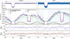 |
Fig. 1 CHEOPS (left) and TESS (right) phase curves of WASP-I2b. Panels a: the total phase curve models overplotted on the detrended and phase-folded data. Panels b: zoom of panel a showing the different components of the total phase curve. The solid blue curve is the total phase curve model for an ellipsoidal planet, while the red dashed curve is for a spherical planet. The solid and dashed green curves represent the best-fit planetary phase variation component (Fp) for the deformed and spherical planets, respectively. The cyan curve is the computed thermal-only 3D GCM for the planet (see Sect. 5.2.2) which shows for CHEOPS that some reflection from the atmosphere is required to reach the amplitude of the green curves. The black curves at the bottom of this panel show the best-fit stellar ellipsoidal variation (FEV) from the deformed (solid) and spherical (dashed) planet model fits. The yellow curve represents the contribution of tidal deformation to the total phase curve, with circles denoting the peaks. Panels c and d: the residuals of the phase curve fits using the ellipsoidal (blue) and spherical (red) planet models. The difference between the models (ellipsoidal–spherical) representing the deformation signature in each passband is overplotted on the spherical model residuals. |
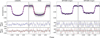 |
Fig. 2 Phase-folded transits of WASP-I2b from the different instruments with the best-fit models overplotted. For each instrument, the 5-min binned residuals for the ellipsoidal (blue) and spherical planet (red) model fits are shown. The difference between both models is again overplotted on the spherical model residuals. |
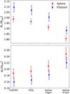 |
Fig. 3 Physical radius and density for WASP-I2b derived from the spherical and ellipsoidal planet model fits. |
Sensitivity of derived Love number on different approaches of modeling limb darkening.
4.2 Impact of limb darkening
As most of the optical band deformation signature is concentrated within the transit phases, the detection is sensitive to the modeling of the limb darkening profile. In the fit for tidal deformation, we used the method described in Sect. 2.2.2 to derive priors on the LDCs based on model intensity profiles from the two spectral synthesis libraries (we call this our fiducial analysis). We also explore two alternative methods to leveraging the generated model intensity profiles, which involve simultaneously fitting the model intensity profiles and the transit observations in order to find the best-fit LD profile.
Alternative-1 : This approach merges the PHOENIX and ATLAS model intensity profiles to create a new joint intensity profile whose lσ uncertainty at each µ encompasses the lσ uncertainty of the individual model profiles (see Fig. B.3b). The joint intensity profile is fitted with the power-2 LD law simultaneously with the transit observations so that a joint likelihood of the suggested limb darkening profile and transit model is obtained (for each passband) at each iteration in our sampling process. This approach allows the joint model intensity profile and transit observations to determine the best-fit limb darkening profile. The parameters of the LD law here have uninformative wide priors since their values are constrained during the joint fit.
Alternative-2 : In this approach, a uniform bound is defined that spans the median of both model intensity profiles (see Fig. B.3c). During the likelihood estimation, each µ point in the suggested limb darkening profile that is anywhere within the defined bounds is assigned zero likelihood. Profile points outside the bound are still acceptable but have lower likelihood values (Gaussian) depending on their distance from the bounds. This approach is agnostic to the eventual choice of limb darkening profile as long as its points are within or close to the bounds defined by both theoretical stellar intensity profiles.
We perform the ellipsoidal planet model fits to the data again using the aforementioned limb darkening alternative approaches and compare the results with our fiducial analysis. The result is given in Table 3 where a consistent value of h2 is derived with the 3 methods, indicating that our fit is robust against the modeling of limb darkening.
5 Atmospheric characterization
Phase curves provide a wealth of information to characterize the atmosphere of a planet such as the day and nightside temperatures, the longitudinal temperature and reflectivity map, and also the efficiency of heat transport among others (see e.g., Cowan & Agol 2011; Shporer 2017; Parmentier & Crossfield 2018). In this section, we infer the atmospheric properties of WASP-l2b from our CHEOPS and TESS phase curve analyses (Sect. 3.3). Unless otherwise stated, the discussion below is based mostly on the phase curve fit using the ellipsoidal planet model. However, we still report the derived parameters for both planet models in Table 2 and we found them to be in agreement within lσ.
5.1 Phase curve constraints
The results of the phase curve fit for the ellipsoidal and spherical planet model fits (Table 2) reveal a larger planet-to-star radius ratio in the CHEOPS band compared to the TESS band, indicating stronger atmospheric opacity in the bluer CHEOPS band. We also measure a significantly lower dayside flux (occultation depth) in CHEOPS compared to TESS. The nightside fluxes in both passbands are consistent with zero at <lσ (2σ upper limits of ~50 ppm). The best-fit phase curves show only marginally significant eastward phase offsets of 9 ± 5° and 6 ± 3° in the CHEOPS and TESS bands, respectively. The low nightside flux and small phase offset in both bands indicate low-efficiency day-night heat redistribution at the atmospheric layers probed by the instruments. This is consistent with the theoretical and observed trend of decreasing phase offset with increasing temperature for ultra-hot Jupiters (Parmentier et al. 2016; Komacek & Showman 2016; Komacek et al. 2017) possibly due to their short radiative timescales (Perna et al. 2012).
5.2 Atmospheric modeling
We model the atmosphere of WASP-l2b by performing ID retrievals on the emission spectrum and computing the forward global circulation model. This will facilitate the proper interpretation of the phase curve, thereby enabling the determination of the relative contribution of both reflection and thermal emission to the observed occultation depths.
5.2.1 1D retrieval
We model the emission spectra of WASP-12b using the open-source PYRAT BAY framework (Cubillos & Blecic 2021) to constrain its atmospheric properties based on the tabulated occultation depth measurements in Hooton et al. (2019, and references therein). This dataset consists of several ground-based, HST/WFC3, and Spitzer measurements spanning 0.5–8 µm. Since reflection is not accounted for in PYRAT BAY, our model only considered the infrared observation (λ > 1.0 µm) to avoid interference from the reflected flux at shorter wavelengths. The retrieved thermal emission spectrum can then be computed including shorter wavelengths to estimate the thermal contribution in the CHEOPS and TESS passbands.
We model the atmosphere of WASP-l2b between 102– l0−9 bar adopting the parametric temperature–pressure (T-P) prescription of Guillot (2010). The parametric model depends on the irradiation temperature Tirr, the mean thermal opacity log κ′, and the ratio of the visible to thermal opacities log γ. For this analysis, we modeled the composition under thermochemi-cal equilibrium, considering the most relevant neutral and ionic species expected for hot-Jupiter atmospheres. The chemistry was parameterized by the abundance of carbon [C/H], oxygen [O/H], and all other metals [M/H] relative to solar-abundance values. The radiative transfer calculation considered HITEMP and Exo-Mol opacity line lists for H2O, CO, CO2, CH4, HCN, NH3, TiO, VO (Rothman et al. 2010; Li et al. 2015; Hargreaves et al. 2020; Harris et al. 2006, 2008; Polyansky et al. 20l8; Coles et al. 20l9; Yurchenko 20l5; McKemmish et al. 20l6, 20l9), which were preprocessed using the REPACK algorithm to extract the dominant line transitions (Cubillos 2017). Additional opacities include the Na and K resonant lines (Burrows et al. 2000), collision-induced absorption from H2–H2 (Borysow et al. 2001; Borysow 2002), Rayleigh opacity from H2, H, and He (Kurucz 1970), and H− free-free and bound-free opacity (John 1988). For the stellar spectrum, we used a synthetic PHOENIX spectrum (Husser et al. 2013) according to the stellar properties (Table 1). Finally, the atmospheric Bayesian retrieval employed a differential-evolution MCMC algorithm implemented in Cubillos et al. (2017) to construct posterior distributions for the atmospheric parameters.
We tested four retrieval scenarios: with and without the Spitzer 5.8 and 8.0 µm data points; and also with and without TiO/VO absorption (since these species may or may not be present in the atmosphere). We found statistically consistent results between all scenarios, thus in the following, we report the results of the retrieval including TiO/VO and all Spitzer observations.
Figure 4 shows the retrieved T–P profile and thermal spectrum, which we extended over the CHEOPS and TESS pass-bands. The retrieval spectral fit is mostly driven by the HST/WFC3 and the Spitzer 3.6 and 4.5 µm observations. The model fits most of the occultation depths relatively well, although several mutually inconsistent measurements lead to a reduced χ2 of 2.9. The observations at wavelengths λ < 2 µm are well fit by a ~3000 K blackbody model, indicating that these bands probe a nearly isothermal region of the atmosphere. The depths at the Spitzer 3.6 µm and 4.5 µm bands imply lower brightness temperatures (~2600 K) than in the HST/WFC3 band, possibly due to absorption by carbon-bearing species. These measurements drive the retrieved model towards a non-inverted T–P profile since these bands probe the upper atmosphere (see contribution function and T–P profile in the right panel of Fig. 4). Previous work by Stevenson et al. (2014a) and Oreshenko et al. (2017) similarly finds a noninverted T–P profile. The retrieval model underestimates the Spitzer 5.8 µm and 8.0 µm which would require higher brightness temperatures of ~3400 K, and thus are inconsistent with the rest of the observations. These Spitzer points have larger uncertainties and are therefore not very constraining in the fit.
In all scenarios, we find insignificant contributions from N-bearing species, which are not expected to be prominent at high-temperature atmospheres in thermochemical equilibrium. Likewise, TiO and VO do not seem to have an impact on the retrieved spectrum, probably because the bluer end of the spectrum (where these molecules absorb the most) is nearly isothermal, which decreases the amplitude of spectral features. On the other hand, C- and O-bearing species (CO, CO2, CH4, H2O) are more prominent. Figure B.4 shows the retrieval posterior distribution, we find super-solar abundances for both carbon and oxygen while keeping mostly C/O > 1 ratios. For other metals, we find sub-solar abundances. These results are consistent with previous retrieval analyses of the WASP-12b emission spectrum (e.g., Oreshenko et al. 2017; Himes & Harrington 2022).
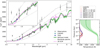 |
Fig. 4 Eclipse spectrum of WASP-12b. Left: observed occultation depths of WASP-12b (gray points) with the CHEOPS and TESS occultation depths are shown as colored diamonds. The best-fit thermal retrieval model and its 1σ uncertainties are overplotted in green while the forward thermal 3D GCM spectrum is plotted in violet. The gray dashed curves show the blackbody model spectra for brightness temperatures of 2600 K, 3000 K, and 3400 K. Right: T–P profile for the retrieval showing a gradual temperature decrease with decreasing pressure depth between 10−1− 10−4 bar indicative of no thermal inversion in the atmosphere of WASP-12 b. The contribution function at each passband is also shown indicating that TESS and CHEOPS essentially probe the same pressure levels within the atmosphere. |
5.2.2 3D global circulation model (GCM)
We also compare the measured occultation depths with the output of a forward 3D GCM that self-consistently calculates the thermal emission from the planet. Here, we use expeRT/MITgcm as introduced by Carone et al. (2020); Schneider et al. (2022). The expeRT/MITgcm uses a pre-calculated grid of correlated-k opacities, where we employ here the S1 spectral resolution as described in Schneider et al. (2022) and opacity sources for Na, K, CH4, H2O, CO2, CO, H2S, HCN, SiO, PH3 and FeH with collision-induced absorption from H2, He and H− and Rayleigh scattering of H2 and He. We omit VO and TiO because our retrievals showed no evidence of a thermal inversion in the upper atmosphere, which would indicate the presence of these molecules. In post-processing, we calculate the thermal emission of the planet for different orbital phases (including the day-side emission) using a wavelength resolution R = 100, where we reduce the spatial resolution of the dayside to 15 degrees in longitude and latitude. During the GCM simulation as well as during post-processing, the abundance of molecules is computed using equilibrium chemistry assuming solar ([Fe/H]=0) metallicity. Thus, we include the effect of thermal ionization of H2 and H2O on our predicted phase curves and dayside emission spectrum.
The dayside emission of the GCM is overplotted in Fig. 4 where we see a good agreement with the retrieval model. In particular, the GCM model correctly predicts that water features are muted in the HST/WFC3 wavelength range (between 1.1 and 1.6 µm) due to a combination of thermal ionization and thus dissociation of H2O over large parts of the dayside and electron opacities that suppress molecular features in this wavelength range. For larger wavelengths, where Spitɀer (and now JWST) is sensitive, molecular features are present again. Although the GCM dayside emission yields smaller amplitude features compared to the best retrieval model, it is still qualitatively in agreement with the available data.
Using the phase-resolved thermal emission spectrum from the GCM, we integrate the flux with the CHEOPS and TESS response functions to obtain the thermal phase variation of the planet in both bands. We overplot the thermal GCM along with the fitted planetary models in Fig. 1. For CHEOPS, the lower amplitude of the thermal GCM compared to the fitted Fp models indicates the need for additional flux from reflection. For TESS , the computed thermal GCM is a good representation of the observed atmospheric phase variation, although the maximum flux and hotspot offset are slightly overestimated; as often seen when comparing GCMs to observations (Parmentier & Crossfield 2018; Zhang et al. 2018). For ultra-hot Jupiters like WASP-12b, it also has been recognized that their daysides are so hot that the gas is dominated by atoms and ions and no longer by molecules like H2O, TiO, and VO. The locally high gas temperatures, therefore, lead to a moderate ionization of the atmosphere (Arcangeli et al. 2018; Parmentier et al. 2018). While expeRT/MITgcm takes the H2O thermal stability into account by calculating a chemical equilibrium model and adjusting abundances accordingly, we did not take into account that this partially ionized flow may couple to the exoplanet’s magnetic field. Which processes dominate a magnetic coupling will depend on the planet’s magnetic field and the local degree of ionization. A partially ionized gas may couple to the magnetic field and some species may, hence, be transported with the flow (Helling et al. 2021). Such interactions may modify the wind flow to dampen the hot spot offset and change the maximum flux (Rogers & Komacek 2014; Beltz et al. 2022), in particular in the infrared (May et al. 2022). In this work, we opted to not add drag to the GCM to mimic the unknown magnetic field in WASP-12 b and minimize the number of uncertainties.
5.3 Albedos and dayside/nightside temperatures
The observed dayside flux in each passband is composed of the thermal emission from the planet and the reflected light by the atmosphere in that passband. The observed flux is thus given (e.g., Esteves et al. 2013; Shporer 2017) as:
 (13)
(13)
For a planet with radius Rp and semi-major axis a, the reflective contribution is determined by the geometric albedo Ag, while the thermal contribution is determined by the emission spectra of the planet and the star 𝓕λ(Tp) and 𝓕λ(Teff), respectively. Therefore, interpreting the measured dayside fluxes requires determining the relative contributions of reflection and thermal emission in the CHEOPS and TESS bands.
As seen in the T–P profile in Fig. 4, CHEOPS and TESS probe similar pressure levels in the atmosphere consistent with black-body dayside temperatures of 2915±25 K and 2821±25 K, respectively. The average measured dayside temperature across both bands is 2868 ± 17 K, in agreement with the effective dayside temperature of 2864 ± 15 K derived in Schwartz et al. (2017). Using the retrieved thermal emission spectra, we calculated the thermal contribution in the CHEOPS and TESS passbands as 205± 10 and 480± 19 ppm, respectively. Subtracting the thermal contribution from the observed occultation depths, we used Eq. (13) to estimate the geometric albedo in the pass-bands. We find Ag = 0.083±0.015 in the CHEOPS band and Ag = 0.010±0.023 in the TESS band, indicating that the atmosphere has non-negligible reflectivity in the CHEOPS band but much lower reflectivity in the TESS band where Ag is consistent with zero with 2σ upper limit of 0.06. The derived Ag values are consistent with the results from the shorter wavelengths of HST /STIS where Bell et al. (2017) found Ag < 0.064.
The derived low geometric albedo of WASP-12 b follows the trend of low reflectivity (A𝑔 ≲ 0.2) of UHJs in the optical to near-infrared transition bands (Mallonn et al. 2019), which is supported by the difficulty in forming condensates at such high temperatures (Parmentier et al. 2018; Wakeford et al. 2017). Perhaps unlikely, but the higher albedo in the CHEOPS band may be due to high-temperature condensates (e.g., silicates, Al2O3, CaTiO3) on the western terminator that have been transported from the nightside. Indeed, Sing et al. (2013) found that the best-fit model to the HST/STIS, HST/WFC3, and Spitɀer transmission spectrum of WASP-12 b was Mie scattering by Al2O3 haze but Bell et al. (2017) ruled out this scenario based on low day-side reflectivity measured in the HST/STIS band. They instead favored thermal emission and Rayleigh scattering from atomic hydrogen and helium.
We used Eq. (13) to convert the measured nightside fluxes to nightside brightness temperatures and obtained 2σ upper limits of Tnight ≃ 2000 K in both passbands (Table 2). This implies a large day-night temperature contrast (>45%) as expected for UHJs due to relatively inefficient heat redistribution (Perna et al. 2012; Komacek et al. 2017). The derived high nightside temperature limit is consistent with the expectation of increasing values as a function of stellar irradiation (Keating et al. 2019) as night clouds disperse for highly irradiated planets.
5.4 Dayside atmospheric variability
Several authors have reported hints of possible time variability in the dayside atmospheric brightness of WASP-12 b due to discrepant secondary eclipse depth measurements obtained at various wavelength bands (see Fig. 4). For example, analyses of two i′-band observations from different ground-based telescopes resulted in an eclipse depth difference of more than 2σ (Hooton et al. 2019) while a pair of V-band observations taken within a month of each other revealed eclipse depths that are discrepant with 4.5σ significance (von Essen et al. 2019). There is also a 2.5σ discrepancy between published z′-band depth measurements (López-Morales et al. 2010; Föhring et al. 2013) and similar level of disagreement in measurements taken around ~2µm (see Hooton et al. 2019), and also at Spitɀer 3.6 µm and 4.5 µm (e.g., Cowan et al. 2012; Stevenson et al. 2014b). Given that the reported eclipse depths have come from different instruments and authors, it is possible that some of the observed disagreements could be due to instrument systematics, observing conditions, telluric contamination in ground-based observations, or even in the analysis of the data. However, Komacek & Showman (2019) showed that the hydrodynamic instabilities in hot Jupiter atmospheres can impact the thermal emission leading to variability at the 2% level in eclipse depth measurements. WASP-12 b can particularly show variability due to magnetohydrodynamic effects in the partially ionized atmosphere (Rogers & Komacek 2014). It remains unclear whether the observed disagreements are astrophysical or due to systematics.
Contrary to these results, the analysis of 4 sectors of TESS data by Wong et al. (2022) found no strong evidence of variability between the individual eclipse measurements, although the largest discrepancy between any two measurements is 3.1 σ. Given the low signal-to-noise of the individual TESS eclipses, they were only able to place 2σ upper limits of 450 ppm and 80 ppm on orbit-to-orbit and month-long variability, respectively.
We further investigate this potential variability with the CHEOPS occultation observations spanning 3 seasons. The analyses of the 26 occultations have been described in Sect. 3.5. Figure 5 shows the derived occultation depths and their 1 σ uncertainties ordered chronologically. The depths derived from the joint fit of occultations with each season of observation are also shown. The individual occultation depths agree with each other within 1σ and also with the joint fit of each season better than 1.2σ. The largest discrepancy between any two depth measurements is 1.8σ while the joint fits for the seasons are in agreement within 1 σ. We search for periodicity in the occultation depths using a Lomb-Scargle periodogram (Lomb 1976; Scargle 1982) and found the highest peak periodicity of 8.3 days to be nonsignificant with a false alarm probability of ~20%. Therefore, we do not find strong evidence for variability in the dayside atmosphere of WASP-12 b at the median depth precision of 120 ppm attained by CHEOPS.
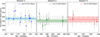 |
Fig. 5 Occultation depth measurements of individual CHEOPS visits in the three observation seasons. The horizontal lines and shaded regions represent the measured depth from jointly fitting all the visits in each season. The depths measured between seasons are consistent within 1σ. The dotted sinusoidal signal is the best-fit periodic signal (P = 8.3) to the depth measurements across all seasons. |
6 Tidal decay
Previous analyses of the transit times of WASP-12 b have clearly shown that the orbit of the planet is decaying due to tidal interaction with the star, causing the planet to lose angular momentum to the star (Maciejewski et al. 2016; Yee et al. 2019; Turner et al. 2021; Wong et al. 2022). The estimate of the planet’s decay rate was possible due to the long baseline of available timing measurements. Since our CHEOPS observations further extend the time baseline, we perform a fit to refine the ephemeris and decay rate of the WASP-12 b by combining our transit and occultation timing measurements given in Table A.5. We combined these CHEOPS transit timings with prior transit and occultation timings compiled by Yee et al. (2019) from various authors and TESS timings derived in Wong et al. (2022).
We model the orbital decay of the planet using a quadratic ephemeris model which gives the transit and occultation times (e.g., Turner et al. 2021) as :
 (14)
(14)
where T0 is the reference transit time closest to the middle of the entire time series, E is the transit epoch, and dP/dE is the orbital decay rate from which the time decay rate  and the decay timescale τ = P/Ṗ can be derived. We used emcee to simultaneously fit Eq. (14) to the transit and occultation times with T0, P, and dP/dE as free parameters. The result from the model fit is given as:
 (15)
(15)
from which we derived:
 (16)
(16)
The decay rate Ṗ derived from our fit including new timing measurements by CHEOPS remains consistent with the estimate of −29.81 ± 0.94 ms yr−1 obtained in Wong et al. (2022) but improves the precision by 12%. Our revised orbital decay timescale τ is slightly shorter but 13% more precise than the value of 3.16 ± 0.1 Myr derived in Wong et al. (2022). Figure 6 shows the transit and occultation timing deviations of WASP-12 b and the orbital decay model fit after subtraction of the best-fit linear ephemeris model.
The rate at which the planet’s orbital energy (Ep) and angular momentum (Lp) are being lost to the star can be calculated (e.g., Yee et al. 2019) as:
 (17)
(17)
The energy is then dissipated inside the star as the tidal oscillations are converted into heat. The efficiency of tidal dissipation is quantified by the modified tidal quality factor of the star Q′★ which can we derive from Ṗ using the constant lag model of Goldreich & Soter (1966) as:
 (18)
(18)
Population studies of stars show that the value of Q′★ ranges between 105−106.5 for hot Jupiter systems and may extend up to 107 for binary star systems (Jackson et al. 2008; Ogilvie 2014). Lower values of Q′★ imply more efficient tidal dissipation. Our derived value in agreement with the value of Q′★ = (1.75±0.12) × 105 derived in Yee et al. (2019). The derived value is on the low end of the range of Q′★ values and implies a much higher dissipation rate for WASP-12 than is expected for a main-sequence star (Turner et al. 2021; Yee et al. 2019). Since the efficiency of tidal dissipation depends also on the structure and evolutionary state of the star, one explanation would be that WASP-l2 is actually a subgiant star capable of such efficient dissipation due to nonlinear breaking of gravity waves close to the center of the star (Weinberg et al. 2017). However, further stellar modeling reports that the observed characteristics of WASP-l2 are consistent with a main-sequence star rather than a subgiant (Bailey & Goodman 2019). Our modeling also confirms a young stellar age of 2.3 Gyr (Sect. 2.2.l).
Tidal decay has not been confirmed for any other exoplanet despite several ultra-hot Jupiter systems having similar planetary and orbital characteristics as WASP-12. Recently, Vissapragada et al. (2022) reported evidence for the tidal decay of Kep1er-1658 b orbiting an evolved star and derived a decay rate of  ms yr−1. However, further observation of this system will be needed to improve the precision of the orbital decay rate. As this is the first reported case of planetary inspiral around an evolved star, its confirmation will give support to the theoretical expectation of planetary engulfment with stellar evolution, which results in the observed dearth of hot Jupiters around evolved stars (Grunblatt et al. 2022). Harre et al. (2023) also reported a 5σ significant measurement of orbital decay for WASP-4 b but found that more observations are required to differentiate between the tidal decay and apsidal precession scenarios.
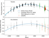 |
Fig. 6 Deviation in the transit (top) and occultation (bottom) timings of WASP-l2b compared to the best-fit linear ephemeris model. The black and green points are published measurements taken from Yee et al. (2019) and Wong et al. (2022), respectively, while the red points are the new CHEOPS timing measurements. |
7 Conclusion
In this work, we have presented a detailed analysis of WASP-12 b using observations by the CHEOPS spacecraft alongside publicly available data from TESS and Spitɀer. We leverage these datasets to put constraints on the shape, atmosphere, and orbital characteristics of the planet. We summarize the main results below·
The large number of CHEOPS visits allowed us to construct a phase curve which we analyzed together with TESS phase curve and Spitɀer transits to constrain the tidal deformation and atmospheric properties of the planet. From our global fit to the datasets, we measured a Love number of
 corresponding to a 3.16 σ detection. This measurement makes WASP-12 b the second planet, after WASP-103 b, where tidal deformation has been significantly detected from the light curve. The 3σ Love number measurements for these planets are still consistent with those of Jupiter despite the strong irradiation of these planets. There is a need to improve the precision of Love number measurements in order to perform comparative interior structure analysis between these highly irradiated, tidally locked planets and the cooler Jupiter. Phase curve observations of such planets with JWST will provide the precisions needed to measure the Love number at ~ 12σ significance, which will in turn better constrain their core mass fractions and interior structures (Akinsanmi et al. 2024);
We significantly measure occultation depths of 333 ± 24 ppm and 493 ± 29 ppm in the CHEOPS and TESS bands, respectively. The nightside fluxes are consistent with zero at both bands. We compared our phase curve with the output of 3D-GCM and found close agreement between them. We measured marginal eastward phase offset of in both bands. We also detected stellar ellipsoidal variation in both pass-bands, which leads to mass estimates that marginally differ from the RV-derived mass at the 1.2–1.8σ level if a spherical planet shape is assumed. However, when we account for tidal deformation, the mass estimates agree with the RV value at < 1σ indicating a preference for the ellipsoidal model;
We model the emission spectrum of WASP-12 b using published occultation depth measurements spanning 0.5–8 µm to derive the thermal profile of the planet. Our best-fit model indicates that CHEOPS and TESS are probing the same pressure level in the atmosphere of WASP-12 b with an average brightness temperature of ~2868 K. We found no evidence of temperature inversion in the atmosphere in agreement with the conclusion from Madhusudhan et al. (2011). We additionally estimate the geometric albedo of the planet and find the planet to be more reflective in the CHEOPS band with Ag = 0.086 ± 0.017 than in TESS with Ag = 0.01 ± 0.023;
Our analysis of the CHEOPS occultations did not show strong evidence of variability in the dayside atmosphere of the planet at the median occultation depth precision of 120 ppm attained by CHEOPS;
Our analysis of the tidal decay of the planet using the new CHEOPS observations refines the orbital decay rate of the planet to −30.13 ± 0.82 ms yr−1 corresponding to a precision improvement of 12% compared to the latest estimates from Wong et al. (2021).
Acknowledgements
CHEOPS is an ESA mission in partnership with Switzerland with important contributions to the payload and the ground segment from Austria, Belgium, France, Germany, Hungary, Italy, Portugal, Spain, Sweden, and the United Kingdom. The CHEOPS Consortium would like to gratefully acknowledge the support received by all the agencies, offices, universities, and industries involved. Their flexibility and willingness to explore new approaches were essential to the success of this mission. BA acknowledges the financial support of the Swiss National Science Foundation under grant number PCEFP2_194576. ML acknowledges support of the Swiss National Science Foundation under grant number PCEFP2_194576. S.C.C.B. acknowledges support from FCT through FCT contracts nr. IF/01312/2014/CP1215/CT0004. LCa and CHe acknowledge support from the European Union H2020-MSCA-ITN-2019 under Grant Agreement no. 860470 (CHAMELEON). P.E.C. is funded by the Austrian Science Fund (FWF) Erwin Schroedinger Fellowship, program J4595-N. ACCa and TWi acknowledge support from STFC consolidated grant numbers ST/R000824/1 and ST/V000861/1, and UKSA grant number ST/R003203/1. GBr, GSc, VSi, LBo, VNa, IPa, GPi, and RRa acknowledge support from CHEOPS ASI-INAF agreement no. 2019-29-HH.0. B.-O.D. acknowledges support from the Swiss State Secretariat for Education, Research and Innovation (SERI) under contract number MB22.00046. ABr was supported by the SNSA. S.G.S. acknowledge support from FCT through FCT contract nr. CEECIND/00826/2018 and POPH/FSE (EC). This work was supported by FCT – Fundação para a Ciência e a Tecnologia through national funds and by FEDER through COMPETE2020 – Programa Operacional Competitividade e Internacionalizacão by these grants: UID/FIS/04434/2019, UIDB/04434/2020, UIDP/04434/2020, PTDC/FIS-AST/32113/2017 and POCI-01-0145-FEDER-032113, PTDC/FIS-AST/28953/2017 and POCI-01-0145-FEDER-028953, PTDC/FIS-AST/28987/2017 and POCI-01-0145-FEDER-028987, O.D.S.D. is supported in the form of work contract (DL 57/2016/CP1364/CT0004) funded by national funds through FCT. YAl acknowledges support from the Swiss National Science Foundation (SNSF) under grant 200020_192038. RAl, DBa, EPa, and IRi acknowledge financial support from the Agencia Estatal de Investigación of the Ministerio de Ciencia e Innovación MCIN/AEI/10.13039/501100011033 and the ERDF “A way of making Europe” through projects PID2019-107061GB-C61, PID2019-107061GB-C66, PID2021-125627OB-C31, and PID2021-125627OB-C32, from the Centre of Excellence “Severo Ochoa” award to the Instituto de Astrofísica de Canarias (CEX2019-000920-S), from the Centre of Excellence “María de Maeztu” award to the Institut de Ciències de l’Espai (CEX2020-001058-M), and from the Generalitat de Catalunya/CERCA programme. X.B., S.C., D.G., M.F. and J.L. acknowledge their role as ESA-appointed CHEOPS science team members. This work has been carried out within the framework of the NCCR PlanetS supported by the Swiss National Science Foundation under grants 51NF40_182901 and 51NF40_205606. This project was supported by the CNES. The Belgian participation to CHEOPS has been supported by the Belgian Federal Science Policy Office (BELSPO) in the framework of the PRODEX Program, and by the University of Liège through an ARC grant for Concerted Research Actions financed by the Wallonia-Brussels Federation. L.D. is an F.R.S.-FNRS Postdoctoral Researcher. This project has received funding from the European Research Council (ERC) under the European Union’s Horizon 2020 research and innovation programme (project FOUR ACES. grant agreement no. 724427). It has also been carried out in the frame of the National Centre for Competence in Research PlanetS supported by the Swiss National Science Foundation (SNSF). D.E. acknowledges financial support from the Swiss National Science Foundation for project 200021_200726. M.F. and C.M.P. gratefully acknowledge the support of the Swedish National Space Agency (DNR 65/19, 174/18). DG gratefully acknowledges financial support from the CRT foundation under Grant No. 2018.2323 “Gaseousor rocky? Unveiling the nature of small worlds”. M.G. is an F.R.S.-FNRS Senior Research Associate. MNG is the ESA CHEOPS Project Scientist and Mission Representative, and as such also responsible for the Guest Observers (GO) Programme. MNG does not relay proprietary information between the GO and Guaranteed Time Observation (GTO) Programmes, and does not decide on the definition and target selection of the GTO Programme. SH gratefully acknowledges CNES funding through the grant 837319. KGI is the ESA CHEOPS Project Scientist and is responsible for the ESA CHEOPS Guest Observers Programme. She does not participate in, or contribute to, the definition of the Guaranteed Time Programme of the CHEOPS mission through which observations described in this paper have been taken, nor to any aspect of target selection for the programme. K.W.F.L. was supported by Deutsche Forschungsgemeinschaft grants RA714/14-1 within the DFG Schwerpunkt SPP 1992, Exploring the Diversity of Extrasolar Planets. This work was granted access to the HPC resources of MesoPSL financed by the Region Ile de France and the project Equip@Meso (reference ANR-10-EQPX-29-01) of the programme Investissements d’Avenir supervised by the Agence Nationale pour la Recherche. AC acknowledges support from PTDC/FIS-AST/7002/2020. PM acknowledges support from STFC research grant number ST/M001040/1. This work was also partially sup rted by a grant from the Simons Foundation (PI Queloz, grant po number 327127). NCSa acknowledges funding by the European Union (ERC, FIERCE,101052347). Views and opinions expressed are however those of the author(s) only and do not necessarily reflect those of the European Union or the European Research Council. Neither the European Union nor the granting authority can be held responsible for them. GyMSz acknowledges the support of the Hungarian National Research, Development and Innovation Office (NKFIH) grant K-125015, a PRODEX Experiment Agreement No. 4000137122, the Lendület LP2018-7/2021 grant of the Hungarian Academy of Science and the support of the city of Szombathely. V.V.G. is an F.R.S-FNRS Research Associate. NAW acknowledges UKSA grant ST/R004838/1.
Appendix A Tables
CHEOPS observation log of WASP-12 . The visit types are either occultation (occ), transit (tra), or phase-curve (PC). βwβr gives the white and red noise correction factor to the flux uncertainties of each visit.
TESS observation log of WASP-12
Spitzer transit observation log of WASP-12
Derived power-2 LDC priors in the different passbands and the posterior from the ellipsoidal and spherical planet model fits.
Derived mid-transit times for the individual CHEOPS transit observations of WASP-12b.
Appendix B Figures
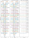 |
Fig. B.1 CHEOPS transit light curves of WASP-12b labeled according to the visit number. Left: The best-fit transit and systematics model is overplotted on the data. Middle: Systematics detrended flux with transit model overplotted. The obtained transit time uncertainty for each visit is shown in seconds. Right: Residuals after subtraction of best-fit transit and systematics model. The 30-min bins and the root-mean-square (rms) of each visit are also shown. |
 |
Fig. B.2 CHEOPS occultation light curves of WASP-12b labeled according to their visit numbers. Left: The best-fit occultation and systematics model is overplotted on the data. Middle: Systematics detrended flux with occultation model overplotted. Right: Residuals after subtraction of best-fit occultation and systematics model. The 30-min bins and the root-mean-square (rms) of each visit are also shown. |
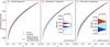 |
Fig. B.3 Different approaches adopted to model the stellar limb darkening using model stellar intensity profiles from the PHOENIX (red) and ATLAS (blue) libraries. The plots illustrate the approaches for the Spitzer 4.5µm passband observations. Panel (a) illustrates our “fiducial” approach where LDCs are generated to be used as priors in the transit model fitting. The black curve shows the fit of the power-2 law to the combined model intensity profiles. The parameter space (gray) allowed by the 1σ uncertainty of the obtained LDCs encompasses both intensity profiles and associated 1σ uncertainties. Panel (b) shows the “alternative-1” approach which merges the PHOENIX and ATLAS model profiles to create a new joint intensity profile (cyan) whose 1σ uncertainties at each µ encompasses the 1σ uncertainty of the individual profiles. This is illustrated in the inset for µ = 0.4. The new joint profile is fitted with an LD law alongside the transit observation at each passband. Panel (c) shows the “alternative-2” approach which similarly combines both intensity profiles but creates a uniform bound (cyan) spanning the median of both profiles such that LD profile points within the bound have equal likelihood but decrease as the profile points deviate from the bound. |
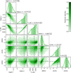 |
Fig. B.4 Posterior distribution of the retrieval using PYRAT BAY with the median and 1σ. |
 |
Fig. B.5 Corner plot showing the posterior probability distributions of the fitted parameters for the spherical planet model (red) and ellipsoidal planet model. Vertical colored lines indicate the median of the distributions while shaded regions define the 68%credible intervals. The different instruments are labeled: CHEOPS (ch), TESS (tess), Spitzer 3.6µm (spl), and Spitzer 4.5µm (sp2). |
References
- Akinsanmi, B., Barros, S. C., Santos, N. C., et al. 2019, A&A, 621, A117 [NASA ADS] [CrossRef] [EDP Sciences] [Google Scholar]
- Akinsanmi, B., Lendl, M., Boué, G., & Barros, S. C. C. 2024, A&A, 682, A15 [NASA ADS] [CrossRef] [EDP Sciences] [Google Scholar]
- Arcangeli, J., Désert, J.-M., Line, M. R., et al. 2018, ApJ, 855, L30 [Google Scholar]
- Bailey, A., & Goodman, J. 2019, MNRAS, 482, 1872 [NASA ADS] [CrossRef] [Google Scholar]
- Barros, S. C. C., Akinsanmi, B., Boué, G., et al. 2022, A&A, 657, A52 [NASA ADS] [CrossRef] [EDP Sciences] [Google Scholar]
- Batygin, K., Bodenheimer, P., & Laughlin, G. 2009, ApJ, 704, L49 [NASA ADS] [CrossRef] [Google Scholar]
- Bell, T. J., Nikolov, N., Cowan, N. B., et al. 2017, ApJ, 847, L2 [Google Scholar]
- Bell, T. J., Zhang, M., Cubillos, P. E., et al. 2019, MNRAS, 489, 1995 [Google Scholar]
- Benz, W., Broeg, C., Fortier, A., et al. 2021, Exp. Astron., 51, 109 [Google Scholar]
- Beltz, H., Rauscher, E., Roman, M. T., & Guilliat, A. 2022, AJ, 163, 35 [NASA ADS] [CrossRef] [Google Scholar]
- Berardo, D., & De Wit, J. 2022, ApJ, 941, 155 [NASA ADS] [CrossRef] [Google Scholar]
- Blackwell, D. E., & Shallis, M. J. 1977, MNRAS, 180, 177 [NASA ADS] [CrossRef] [Google Scholar]
- Bonfanti, A., Ortolani, S., Piotto, G., & Nascimbeni, V. 2015, A&A, 575, A18 [NASA ADS] [CrossRef] [EDP Sciences] [Google Scholar]
- Bonfanti, A., Ortolani, S., & Nascimbeni, V. 2016, A&A, 585, A5 [NASA ADS] [CrossRef] [EDP Sciences] [Google Scholar]
- Bonfanti, A., Delrez, L., Hooton, M. J., et al. 2021, A&A, 646, A157 [EDP Sciences] [Google Scholar]
- Borysow, A. 2002, A&A, 390, 779 [NASA ADS] [CrossRef] [EDP Sciences] [Google Scholar]
- Borysow, A., Jorgensen, U. G., & Fu, Y. 2001, J. Quant. Spec. Radiat. Transf., 68, 235 [NASA ADS] [CrossRef] [Google Scholar]
- Brandeker, A., Heng, K., Lendl, M., et al. 2022, A&A, 659, L4 [NASA ADS] [CrossRef] [EDP Sciences] [Google Scholar]
- Buhler, P. B., Knutson, H. A., Batygin, K., et al. 2016, ApJ, 821, 26 [CrossRef] [Google Scholar]
- Burrows, A., Marley, M. S., & Sharp, C. M. 2000, ApJ, 531, 438 [NASA ADS] [CrossRef] [Google Scholar]
- Burton, J. R., Watson, C. A., Fitzsimmons, A., et al. 2014, ApJ, 789, 113 [NASA ADS] [CrossRef] [Google Scholar]
- Carone, L., Baeyens, R., Mollière, P., et al. 2020, MNRAS, 496, 3582 [NASA ADS] [CrossRef] [Google Scholar]
- Claret, A. 2017, A&A, 600, A30 [NASA ADS] [CrossRef] [EDP Sciences] [Google Scholar]
- Claret, A. 2021, RNAAS, 5, 13 [NASA ADS] [Google Scholar]
- Claret, A., & Bloemen, S. 2011, A&A, 529, A75 [NASA ADS] [CrossRef] [EDP Sciences] [Google Scholar]
- Claret, A., & Southworth, J. 2022, A&A, 664, A128 [NASA ADS] [CrossRef] [EDP Sciences] [Google Scholar]
- Coles, P. A., Yurchenko, S. N., & Tennyson, J. 2019, MNRAS, 490, 4638 [CrossRef] [Google Scholar]
- Collins, K. A., Kielkopf, J. F., & Stassun, K. G. 2017, AJ, 153 [Google Scholar]
- Correia, A. C. M. 2014, A&A, 570, A5 [NASA ADS] [CrossRef] [EDP Sciences] [Google Scholar]
- Correia, A. C. M., & Rodríguez, A. 2013, ApJ, 767, 128 [NASA ADS] [CrossRef] [Google Scholar]
- Correia, A. C., Boué, G., Laskar, J., & Rodríguez, A. 2014, A&A, 571, A50 [NASA ADS] [CrossRef] [EDP Sciences] [Google Scholar]
- Cowan, N. B., & Agol, E. 2011, ApJ, 729, 54 [Google Scholar]
- Cowan, N. B., Machalek, P., Croll, B., et al. 2012, ApJ, 747, 82 [Google Scholar]
- Cubillos, P. E. 2017, ApJ, 850, 32 [CrossRef] [Google Scholar]
- Cubillos, P. E., & Blecic, J. 2021, MNRAS, 505, 2675 [NASA ADS] [CrossRef] [Google Scholar]
- Cubillos, P., Harrington, J., Loredo, T. J., et al. 2017, AJ, 153, 3 [Google Scholar]
- Daylan, T., Günther, M. N., Mikal-Evans, T., et al. 2021, AJ, 161, 131 [NASA ADS] [CrossRef] [Google Scholar]
- Deline, A., Hooton, M. J., Lendl, M., et al. 2022, A&A, 659, A74 [NASA ADS] [CrossRef] [EDP Sciences] [Google Scholar]
- Delrez, L., Leleu, A., Brandeker, A., et al. 2023, J. Laskar, 10, 51 [Google Scholar]
- Demory, B.-O., Gillon, M., de Wit, J., et al. 2016a, Nature, 532, 207 [NASA ADS] [CrossRef] [Google Scholar]
- Demory, B.-O., Gillon, M., Madhusudhan, N., & Queloz, D. 2016b, MNRAS, 455, 2018 [NASA ADS] [CrossRef] [Google Scholar]
- Demory, B.-O., Sulis, S., Meier Valdés, E., et al. 2023, A&A, 669, A64 [NASA ADS] [CrossRef] [EDP Sciences] [Google Scholar]
- Dermott, S. F. 1979, Icarus, 37, 310 [NASA ADS] [CrossRef] [Google Scholar]
- Durante, D., Parisi, M., Serra, D., et al. 2020, Geophys. Res. Lett., 47, e2019GL086572 [CrossRef] [Google Scholar]
- Ehrenreich, D., Delrez, L., Akinsanmi, B., et al. 2023, A&A, 671, A154 [NASA ADS] [CrossRef] [EDP Sciences] [Google Scholar]
- Espinoza, N., & Jordán, A. 2015, MNRAS, 450, 1879 [Google Scholar]
- Esteves, L. J., De Mooij, E. J. W., & Jayawardhana, R. 2013, ApJ, 772, 51 [NASA ADS] [CrossRef] [Google Scholar]
- Föhring, D., Dhillon, V. S., Madhusudhan, N., et al. 2013, MNRAS, 435, 2268 [CrossRef] [Google Scholar]
- Foreman-Mackey, D., Hogg, D. W., Lang, D., & Goodman, J. 2013, PASP, 125, 306 [Google Scholar]
- Fossati, L., Haswell, C. A., Froning, C. S., et al. 2010, ApJ, 714, L222 [Google Scholar]
- Gaia Collaboration (Vallenari, A., et al.) 2023, A&A, 674, A1 [NASA ADS] [CrossRef] [EDP Sciences] [Google Scholar]
- Gillon, M., Triaud, A. H. M. J., Fortney, J. J., et al. 2012, A&A, 542, A4 [NASA ADS] [CrossRef] [EDP Sciences] [Google Scholar]
- Goldreich, P., & Soter, S. 1966, Icarus, 5, 375 [Google Scholar]
- Grunblatt, S. K., Saunders, N., Sun, M., et al. 2022, AJ, 163, 120 [NASA ADS] [CrossRef] [Google Scholar]
- Guillot, T. 2010, A&A, 520, A27 [NASA ADS] [CrossRef] [EDP Sciences] [Google Scholar]
- Hargreaves, R. J., Gordon, I. E., Rey, M., et al. 2020, ApJS, 247, 55 [NASA ADS] [CrossRef] [Google Scholar]
- Harre, J.-V., Smith, A. M. S., Barros, S. C. C., et al. 2023, A&A, 669, A124 [NASA ADS] [CrossRef] [EDP Sciences] [Google Scholar]
- Harris, G. J., Tennyson, J., Kaminsky, B. M., Pavlenko, Y. V., & Jones, H. R. A. 2006, MNRAS, 367, 400 [Google Scholar]
- Harris, G. J., Larner, F. C., Tennyson, J., et al. 2008, MNRAS, 390, 143 [NASA ADS] [CrossRef] [Google Scholar]
- Hebb, L., Collier-Cameron, A., Loeillet, B., et al. 2008, ApJ, 693, 1920 [Google Scholar]
- Hellard, H., Csizmadia, S., Padovan, S., et al. 2019, ApJ, 878, 119 [NASA ADS] [CrossRef] [Google Scholar]
- Helling, C., Gourbin, P., Woitke, P., & Parmentier, V. 2019, A&A, 626, A133 [NASA ADS] [CrossRef] [EDP Sciences] [Google Scholar]
- Helling, C., Worters, M., Samra, D., Molaverdikhani, K., & Iro, N. 2021, A&A, 648, A80 [NASA ADS] [CrossRef] [EDP Sciences] [Google Scholar]
- Hestroffer, D. 1997, A&A, 327, 199 [NASA ADS] [Google Scholar]
- Himes, M. D., & Harrington, J. 2022, ApJ, 931, 86 [NASA ADS] [CrossRef] [Google Scholar]
- Hooton, M. J., de Mooij, E. J. W., Watson, C. A., et al. 2019, MNRAS, 486, 2397 [NASA ADS] [CrossRef] [Google Scholar]
- Hooton, M. J., Hoyer, S., Kitzmann, D., et al. 2022, A&A, 658, A75 [NASA ADS] [CrossRef] [EDP Sciences] [Google Scholar]
- Hoyer, S., Guterman, P., Demangeon, O., et al. 2020, A&A, 635, A24 [NASA ADS] [CrossRef] [EDP Sciences] [Google Scholar]
- Husser, T.-O., Wende-von Berg, S., Dreizler, S., et al. 2013, A&A, 553, A6 [NASA ADS] [CrossRef] [EDP Sciences] [Google Scholar]
- Hut, P. 1980, A&A, 92, 167 [NASA ADS] [Google Scholar]
- Ingalls, J. G., Krick, J. E., Carey, S. J., et al. 2012, Proc. SPIE, 8442, 84421Y [NASA ADS] [CrossRef] [Google Scholar]
- Jackson, B., Greenberg, R., & Barnes, R. 2008, ApJ, 681, 1631 [NASA ADS] [CrossRef] [Google Scholar]
- John, T. L. 1988, A&A, 193, 189 [NASA ADS] [Google Scholar]
- Jones, K., Morris, B. M., Demory, B.-O., et al. 2022, A&A, 666, A118 [NASA ADS] [CrossRef] [EDP Sciences] [Google Scholar]
- Kass, R. E., & Raftery, A. E. 1995, J. Am. Stat. Assoc., 90, 773 [Google Scholar]
- Keating, D., Cowan, N. B., & Dang, L. 2019, Nat. Astron., 3, 1092 [NASA ADS] [CrossRef] [Google Scholar]
- Kellermann, C., Becker, A., & Redmer, R. 2018, A&A, 615, 39 [Google Scholar]
- Komacek, T. D., & Showman, A. P. 2016, ApJ, 821, 16 [CrossRef] [Google Scholar]
- Komacek, T. D., & Showman, A. P. 2019, ApJ, 888, 2 [NASA ADS] [CrossRef] [Google Scholar]
- Komacek, T. D., Showman, A. P., & Tan, X. 2017, ApJ, 835, 198 [NASA ADS] [CrossRef] [Google Scholar]
- Kramm, U., Nettelmann, N., Redmer, R., & Stevenson, D. J. 2011, A&A, 528, A18 [NASA ADS] [CrossRef] [EDP Sciences] [Google Scholar]
- Kramm, U., Nettelmann, N., Fortney, J. J., Neuhäuser, R., & Redmer, R. 2012, A&A, 538, A146 [NASA ADS] [CrossRef] [EDP Sciences] [Google Scholar]
- Kreidberg, L. 2015, PASP, 127, 1161 [Google Scholar]
- Kreidberg, L., Line, M. R., Parmentier, V., et al. 2018, AJ, 156, 17 [NASA ADS] [CrossRef] [Google Scholar]
- Kurucz, R. L. 1970, SAO Special Report, 309 [Google Scholar]
- Kurucz, R. L. 1993, SYNTHE spectrum synthesis programs and line data (Cambridge, MA, USA: Smithsonian Astrophysical Observatory) [Google Scholar]
- Lainey, V., Jacobson, R. A., Tajeddine, R., et al. 2017, Icarus, 281, 286 [Google Scholar]
- Leconte, J., Lai, D., & Chabrier, G. 2011a, A&A, 536, C1 [NASA ADS] [CrossRef] [EDP Sciences] [Google Scholar]
- Leconte, J., Lai, D., & Chabrier, G. 2011b, A&A, 528, A41 [NASA ADS] [CrossRef] [EDP Sciences] [Google Scholar]
- Lendl, M., Cubillos, P. E., Hagelberg, J., et al. 2017, A&A, 606 [Google Scholar]
- Lendl, M., Csizmadia, S., Deline, A., et al. 2020, A&A, 643, A94 [EDP Sciences] [Google Scholar]
- Li, G., Gordon, I. E., Rothman, L. S., et al. 2015, ApJS, 216, 15 [NASA ADS] [CrossRef] [Google Scholar]
- Lightkurve Collaboration (Cardoso, L., et al.) 2018, Astrophysics Source Code Library [record ascl:1812.013] [Google Scholar]
- Loeb, A., & Gaudi, B. S. 2003, ApJ, 588, L117 [Google Scholar]
- Lomb, N. R. 1976, Astrophys. Space Sci., 39, 447 [Google Scholar]
- López-Morales, M., Coughlin, J. L., Sing, D. K., et al. 2010, ApJL, 716, L36 [CrossRef] [Google Scholar]
- Love, A. E. H. 1911, Nature, 89, 471 [Google Scholar]
- Maciejewski, G., Dimitrov, D., Fernández, M., et al. 2016, A&A, 588, L6 [NASA ADS] [CrossRef] [EDP Sciences] [Google Scholar]
- Madhusudhan, N., Harrington, J., Stevenson, K. B., et al. 2011, Nature, 469, 64 [NASA ADS] [CrossRef] [Google Scholar]
- Mallonn, M., Köhler, J., Alexoudi, X., et al. 2019, A&A, 624, A62 [NASA ADS] [CrossRef] [EDP Sciences] [Google Scholar]
- Marigo, P., Girardi, L., Bressan, A., et al. 2017, ApJ, 835, 77 [Google Scholar]
- Maxted, P. F. L. 2016, A&A, 591, A111 [NASA ADS] [CrossRef] [EDP Sciences] [Google Scholar]
- May, E. M., Stevenson, K. B., Bean, J. L., et al. 2022, AJ, 163, 256 [NASA ADS] [CrossRef] [Google Scholar]
- McKemmish, L. K., Yurchenko, S. N., & Tennyson, J. 2016, MNRAS, 463, 771 [NASA ADS] [CrossRef] [Google Scholar]
- McKemmish, L. K., Masseron, T., Hoeijmakers, H. J., et al. 2019, MNRAS, 488, 2836 [Google Scholar]
- Mendonça, J. M., Malik, M., Demory, B.-O., & Heng, K. 2018, AJ, 155, 150 [Google Scholar]
- Morello, G., Tsiaras, A., Howarth, I. D., & Homeier, D. 2017, AJ, 154, 111 [NASA ADS] [CrossRef] [Google Scholar]
- Morris, B. M., Delrez, L., Brandeker, A., et al. 2021a, A&A, 653, A17 [NASA ADS] [CrossRef] [EDP Sciences] [Google Scholar]
- Morris, B. M., Heng, K., Brandeker, A., Swan, A., & Lendl, M. 2021b, A&A, 651, L12 [NASA ADS] [CrossRef] [EDP Sciences] [Google Scholar]
- Ogilvie, G. I. 2014, ArA&A, 52, 171 [NASA ADS] [CrossRef] [Google Scholar]
- Oreshenko, M., Lavie, B., Grimm, S. L., et al. 2017, ApJ, 847, L3 [NASA ADS] [CrossRef] [Google Scholar]
- Parmentier, V., & Crossfield, I. J. M. 2018, in Handbook of Exoplanets (Cham: Springer International Publishing), 1419 [CrossRef] [Google Scholar]
- Parmentier, V., Fortney, J. J., Showman, A. P., Morley, C., & Marley, M. S. 2016, ApJ, 828, 22 [Google Scholar]
- Parmentier, V., Line, M. R., Bean, J. L., et al. 2018, A&A, 617, A110 [NASA ADS] [CrossRef] [EDP Sciences] [Google Scholar]
- Parviainen, H., Wilson, T. G., Lendl, M., et al. 2022, A&A, 668, A93 [NASA ADS] [CrossRef] [EDP Sciences] [Google Scholar]
- Patel, J. A., & Espinoza, N. 2022, AJ, 163, 228 [NASA ADS] [CrossRef] [Google Scholar]
- Perna, R., Heng, K., & Pont, F. 2012, ApJ, 751, 59 [NASA ADS] [CrossRef] [Google Scholar]
- Polyansky, O. L., Kyuberis, A. A., Zobov, N. F., et al. 2018, MNRAS, 480, 2597 [NASA ADS] [CrossRef] [Google Scholar]
- Ragozzine, D., & Wolf, A. S. 2009, ApJ, 698, 1778 [Google Scholar]
- Rogers, T. M., & Komacek, T. D. 2014, ApJ, 794, 132 [NASA ADS] [CrossRef] [Google Scholar]
- Rothman, L. S., Gordon, I. E., Barber, R. J., et al. 2010, J. Quant. Spec. Radiat. Transf., 111, 2139 [NASA ADS] [CrossRef] [Google Scholar]
- Salmon, S. J. A. J., Van Grootel, V., Buldgen, G., Dupret, M. A., & Eggenberger, P. 2021, A&A, 646, A7 [NASA ADS] [CrossRef] [EDP Sciences] [Google Scholar]
- Santos, N. C., Sousa, S. G., Mortier, A., et al. 2013, A&A, 556, A150 [NASA ADS] [CrossRef] [EDP Sciences] [Google Scholar]
- Scargle, J. D. 1982, ApJ, 263, 835 [Google Scholar]
- Schanche, N., Hébrard, G., Collier Cameron, A., et al. 2020, MNRAS, 499, 428 [NASA ADS] [CrossRef] [Google Scholar]
- Schneider, A. D., Carone, L., Decin, L., et al. 2022, A&A, 664, A56 [NASA ADS] [CrossRef] [EDP Sciences] [Google Scholar]
- Schwartz, J. C., Kashner, Z., Jovmir, D., & Cowan, N. B. 2017, ApJ, 850, 154 [Google Scholar]
- Scuflaire, R., Théado, S., Montalbán, J., et al. 2008, Ap&SS, 316, 83 [Google Scholar]
- Shporer, A. 2017, PASP, 129, 072001 [Google Scholar]
- Shporer, A., Wong, I., Huang, C. X., et al. 2019, AJ, 157, 178 [Google Scholar]
- Sing, D. K., Lecavelier des Etangs, A., Fortney, J. J., et al. 2013, MNRAS, 436, 2956 [NASA ADS] [CrossRef] [Google Scholar]
- Skrutskie, M. F., Cutri, R. M., Stiening, R., et al. 2006, AJ, 131, 1163 [NASA ADS] [CrossRef] [Google Scholar]
- Smith, J. C., Stumpe, M. C., Van Cleve, J. E., et al. 2012, PASP, 124, 1000 [Google Scholar]
- Sneden, C. A. 1973, PhD thesis, The University of Texas at Austin, USA [Google Scholar]
- Sousa, S. G., Santos, N. C., Israelian, G., Mayor, M., & Monteiro, M. J. P. F. G. 2007, A&A, 469, 783 [NASA ADS] [CrossRef] [EDP Sciences] [Google Scholar]
- Sousa, S. G., Santos, N. C., Mayor, M., et al. 2008, A&A, 487, 373 [NASA ADS] [CrossRef] [EDP Sciences] [Google Scholar]
- Sousa, S. G., Santos, N. C., Adibekyan, V., Delgado-Mena, E., & Israelian, G. 2015, A&A, 577, A67 [NASA ADS] [CrossRef] [EDP Sciences] [Google Scholar]
- Sousa, S. G., Adibekyan, V., Delgado-Mena, E., et al. 2018, A&A, 620, A58 [NASA ADS] [CrossRef] [EDP Sciences] [Google Scholar]
- Sousa, S. G., Adibekyan, V., Delgado-Mena, E., et al. 2021, A&A, 656, A53 [NASA ADS] [CrossRef] [EDP Sciences] [Google Scholar]
- Speagle, J. S. 2020, MNRAS, 493, 3132 [Google Scholar]
- Stevenson, K. B., Harrington, J., Fortney, J. J., et al. 2012, ApJ, 754, 136 [Google Scholar]
- Stevenson, K. B., Bean, J. L., Fabrycky, D., & Kreidberg, L. 2014, ApJ, 796, 32 [NASA ADS] [CrossRef] [Google Scholar]
- Stevenson, K. B., Bean, J. L., Madhusudhan, N., & Harrington, J. 2014a, ApJ, 791, 36 [NASA ADS] [CrossRef] [Google Scholar]
- Stevenson, K. B., Bean, J. L., Seifahrt, A., et al. 2014b, AJ, 147, 161 [NASA ADS] [CrossRef] [Google Scholar]
- Stumpe, M. C., Smith, J. C., Van Cleve, J. E., et al. 2012, PASP, 124, 985 [Google Scholar]
- Swain, M., Deroo, P., Tinetti, G., et al. 2013, Icarus, 225, 432 [NASA ADS] [CrossRef] [Google Scholar]
- Turner, J. D., Ridden-Harper, A., & Jayawardhana, R. 2021, AJ, 161, 72 [NASA ADS] [CrossRef] [Google Scholar]
- Vissapragada, S., Chontos, A., Greklek-McKeon, M., et al. 2022, ApJ, 941, L31 [NASA ADS] [CrossRef] [Google Scholar]
- von Essen, C., Stefansson, G., Mallonn, M., et al. 2019, A&A, 628, A115 [NASA ADS] [CrossRef] [EDP Sciences] [Google Scholar]
- Wahl, S. M., Thorngren, D., Lu, T., & Militzer, B. 2021, ApJ, 921, 105 [NASA ADS] [CrossRef] [Google Scholar]
- Wakeford, H. R., Visscher, C., Lewis, N. K., et al. 2017, MNRAS, 464, 4247 [NASA ADS] [CrossRef] [Google Scholar]
- Weinberg, N. N., Sun, M., Arras, P., & Essick, R. 2017, ApJ, 849, L11 [Google Scholar]
- Winn, J. N., Holman, M. J., Torres, G., et al. 2008, ApJ, 683, 1076 [Google Scholar]
- Woitke, P., Helling, C., Hunter, G. H., et al. 2018, A&A, 614, A1 [NASA ADS] [CrossRef] [EDP Sciences] [Google Scholar]
- Wong, I., Kitzmann, D., Shporer, A., et al. 2021, AJ, 162, 127 [NASA ADS] [CrossRef] [Google Scholar]
- Wong, I., Shporer, A., Vissapragada, S., et al. 2022, AJ, 163, 175 [NASA ADS] [CrossRef] [Google Scholar]
- Wright, E. L., Eisenhardt, P. R. M., Mainzer, A. K., et al. 2010, AJ, 140, 1868 [Google Scholar]
- Yee, S. W., Winn, J. N., Knutson, H. A., et al. 2019, ApJ, 888, L5 [Google Scholar]
- Yurchenko, S. N. 2015, J. Quant. Spec. Radiat. Transf., 152, 28 [NASA ADS] [CrossRef] [Google Scholar]
- Zhang, M., Knutson, H. A., Kataria, T., et al. 2018, AJ, 155, 83 [Google Scholar]
- Zharkov, V. N., & Trubitsyn, V. P. 1978, Physics of Planetary Interiors, Astronomy and Astrophysics Series (Tuscon, AZ: Pachart) [Google Scholar]
Implemented with the scipy.interpolate.LSQUnivariateSpline and scipy.interpolate.LSQBivariateSpline python classes.
The latest version, ARES v2, can be downloaded at https://github.com/sousasag/ARES
PAdova and TRieste Stellar Evolutionary Code: http://stev.oapd.inaf.it/cgi-bin/cmd
This relation also satisfies the condition in the linear theory of figures (Zharkov & Trubitsyn 1978; Dermott 1979) that a synchronously rotating body in hydrostatic equilibrium subjected to both rotation and tidal forces deforms such that (r2 − r3)/(r1 − r3) = 1 /4.
Rv of an ellipsoidal planet is always larger than the spherical planet transit radius since only a small part of the long axis is projected during transit. However, for the spherical planet, Rv is equivalent to the spherical planet transit radius.
Our code actually transforms Eq. (10) as a function of Fd and Fn instead of Fmax and Fmin.
All Tables
Sensitivity of derived Love number on different approaches of modeling limb darkening.
CHEOPS observation log of WASP-12 . The visit types are either occultation (occ), transit (tra), or phase-curve (PC). βwβr gives the white and red noise correction factor to the flux uncertainties of each visit.
Derived power-2 LDC priors in the different passbands and the posterior from the ellipsoidal and spherical planet model fits.
Derived mid-transit times for the individual CHEOPS transit observations of WASP-12b.
All Figures
|
Fig. 1 CHEOPS (left) and TESS (right) phase curves of WASP-I2b. Panels a: the total phase curve models overplotted on the detrended and phase-folded data. Panels b: zoom of panel a showing the different components of the total phase curve. The solid blue curve is the total phase curve model for an ellipsoidal planet, while the red dashed curve is for a spherical planet. The solid and dashed green curves represent the best-fit planetary phase variation component (Fp) for the deformed and spherical planets, respectively. The cyan curve is the computed thermal-only 3D GCM for the planet (see Sect. 5.2.2) which shows for CHEOPS that some reflection from the atmosphere is required to reach the amplitude of the green curves. The black curves at the bottom of this panel show the best-fit stellar ellipsoidal variation (FEV) from the deformed (solid) and spherical (dashed) planet model fits. The yellow curve represents the contribution of tidal deformation to the total phase curve, with circles denoting the peaks. Panels c and d: the residuals of the phase curve fits using the ellipsoidal (blue) and spherical (red) planet models. The difference between the models (ellipsoidal–spherical) representing the deformation signature in each passband is overplotted on the spherical model residuals. |
| In the text | |
|
Fig. 2 Phase-folded transits of WASP-I2b from the different instruments with the best-fit models overplotted. For each instrument, the 5-min binned residuals for the ellipsoidal (blue) and spherical planet (red) model fits are shown. The difference between both models is again overplotted on the spherical model residuals. |
| In the text | |
|
Fig. 3 Physical radius and density for WASP-I2b derived from the spherical and ellipsoidal planet model fits. |
| In the text | |
|
Fig. 4 Eclipse spectrum of WASP-12b. Left: observed occultation depths of WASP-12b (gray points) with the CHEOPS and TESS occultation depths are shown as colored diamonds. The best-fit thermal retrieval model and its 1σ uncertainties are overplotted in green while the forward thermal 3D GCM spectrum is plotted in violet. The gray dashed curves show the blackbody model spectra for brightness temperatures of 2600 K, 3000 K, and 3400 K. Right: T–P profile for the retrieval showing a gradual temperature decrease with decreasing pressure depth between 10−1− 10−4 bar indicative of no thermal inversion in the atmosphere of WASP-12 b. The contribution function at each passband is also shown indicating that TESS and CHEOPS essentially probe the same pressure levels within the atmosphere. |
| In the text | |
|
Fig. 5 Occultation depth measurements of individual CHEOPS visits in the three observation seasons. The horizontal lines and shaded regions represent the measured depth from jointly fitting all the visits in each season. The depths measured between seasons are consistent within 1σ. The dotted sinusoidal signal is the best-fit periodic signal (P = 8.3) to the depth measurements across all seasons. |
| In the text | |
|
Fig. 6 Deviation in the transit (top) and occultation (bottom) timings of WASP-l2b compared to the best-fit linear ephemeris model. The black and green points are published measurements taken from Yee et al. (2019) and Wong et al. (2022), respectively, while the red points are the new CHEOPS timing measurements. |
| In the text | |
|
Fig. B.1 CHEOPS transit light curves of WASP-12b labeled according to the visit number. Left: The best-fit transit and systematics model is overplotted on the data. Middle: Systematics detrended flux with transit model overplotted. The obtained transit time uncertainty for each visit is shown in seconds. Right: Residuals after subtraction of best-fit transit and systematics model. The 30-min bins and the root-mean-square (rms) of each visit are also shown. |
| In the text | |
|
Fig. B.2 CHEOPS occultation light curves of WASP-12b labeled according to their visit numbers. Left: The best-fit occultation and systematics model is overplotted on the data. Middle: Systematics detrended flux with occultation model overplotted. Right: Residuals after subtraction of best-fit occultation and systematics model. The 30-min bins and the root-mean-square (rms) of each visit are also shown. |
| In the text | |
|
Fig. B.3 Different approaches adopted to model the stellar limb darkening using model stellar intensity profiles from the PHOENIX (red) and ATLAS (blue) libraries. The plots illustrate the approaches for the Spitzer 4.5µm passband observations. Panel (a) illustrates our “fiducial” approach where LDCs are generated to be used as priors in the transit model fitting. The black curve shows the fit of the power-2 law to the combined model intensity profiles. The parameter space (gray) allowed by the 1σ uncertainty of the obtained LDCs encompasses both intensity profiles and associated 1σ uncertainties. Panel (b) shows the “alternative-1” approach which merges the PHOENIX and ATLAS model profiles to create a new joint intensity profile (cyan) whose 1σ uncertainties at each µ encompasses the 1σ uncertainty of the individual profiles. This is illustrated in the inset for µ = 0.4. The new joint profile is fitted with an LD law alongside the transit observation at each passband. Panel (c) shows the “alternative-2” approach which similarly combines both intensity profiles but creates a uniform bound (cyan) spanning the median of both profiles such that LD profile points within the bound have equal likelihood but decrease as the profile points deviate from the bound. |
| In the text | |
|
Fig. B.4 Posterior distribution of the retrieval using PYRAT BAY with the median and 1σ. |
| In the text | |
|
Fig. B.5 Corner plot showing the posterior probability distributions of the fitted parameters for the spherical planet model (red) and ellipsoidal planet model. Vertical colored lines indicate the median of the distributions while shaded regions define the 68%credible intervals. The different instruments are labeled: CHEOPS (ch), TESS (tess), Spitzer 3.6µm (spl), and Spitzer 4.5µm (sp2). |
| In the text | |
Current usage metrics show cumulative count of Article Views (full-text article views including HTML views, PDF and ePub downloads, according to the available data) and Abstracts Views on Vision4Press platform.
Data correspond to usage on the plateform after 2015. The current usage metrics is available 48-96 hours after online publication and is updated daily on week days.
Initial download of the metrics may take a while.