| Issue |
A&A
Volume 629, September 2019
|
|
|---|---|---|
| Article Number | A63 | |
| Number of page(s) | 19 | |
| Section | Interstellar and circumstellar matter | |
| DOI | https://doi.org/10.1051/0004-6361/201935882 | |
| Published online | 06 September 2019 | |
Synthetic observations of dust emission and polarisation of Galactic cold clumps
1
Department of Physics, PO Box 64, University of Helsinki,
00014 Helsinki,
Finland
e-mail: mika.juvela@helsinki.fi
2
ICREA & Institut de Ciències del Cosmos, Universitat de Barcelona, IEEC-UB,
Martí Franquès 1, 08028 Barcelona, Spain
3
Université de Toulouse, UPS-OMP, IRAP,
31028 Toulouse Cedex 4, France
4
CNRS, IRAP, 9 Av. colonel Roche, BP 44346,
31028 Toulouse Cedex 4, France
5
Institut de Ciències del Cosmos, Universitat de Barcelona, IEEC-UB,
Martí Franquès 1, 08028 Barcelona, Spain
Received:
13
May
2019
Accepted:
7
August
2019
Context. The Planck Catalogue of Galactic Cold Clumps (PGCC) contains over 13 000 sources that are detected based on their cold dust signature. They are believed to consist of a mixture of quiescent, pre-stellar, and already star-forming objects within molecular clouds.
Aims. We extracted PGCC-type objects from cloud simulations and examined their physical and polarisation properties. The comparison with the PGCC catalogue helps to characterise the properties of this large sample of Galactic objects and, conversely, provides valuable tests for numerical simulations of large volumes of the interstellar medium and the evolution towards pre-stellar cores.
Methods. We used several magnetohydrodynamical simulation snapshots to define the density field of our model clouds. Sub-millimetre images of the surface brightness and polarised signal were obtained with radiative transfer calculations. We examined the statistics of synthetic cold clump catalogues extracted with methods similar to the PGCC. We also examined the variations of the polarisation fraction p in the clumps.
Results. The clump sizes, aspect ratios, and temperatures in the synthetic catalogue are similar to the PGCC. The fluxes and column densities of synthetic clumps are smaller by a factor of a few. Rather than with an increased dust opacity, this could be explained by increasing the average column density of the model by a factor of two to three, close to N(H2) = 1022 cm−2. When the line of sight is parallel to the mean magnetic field, the polarisation fraction tends to increase towards the clump centres, which is contrary to observations. When the field is perpendicular, the polarisation fraction tends to decrease towards the clumps, but the drop in p is small (e.g. from p ~8% to p ~7%).
Conclusions. Magnetic field geometry reduces the polarisation fraction in the simulated clumps by only Δp ~1% on average. The larger drop seen towards the actual PGCC clumps therefore suggests some loss of grain alignment in the dense medium, such as predicted by the radiative torque mechanism. The statistical study is not able to quantify dust opacity changes at the scale of the PGCC clumps.
Key words: ISM: clouds / infrared: ISM / submillimeter: ISM / dust, extinction / stars: formation / stars: protostars
© ESO 2019
1 Introduction
The Planck Catalogue of Galactic Cold Clumps (PGCC; Planck Collaboration XXVIII 2016) contains over 13 000 cold Galactic sources that were detected using Planck sub-millimetre observations (Planck Collaboration I 2016) and the 100 μm data from the Infrared Astronomical Satellite (IRAS) survey (Neugebauer et al. 1984). The source extraction was not based on the absolute brightness of the sources but on the cold dust signature, that is obtained by subtracting the signal of warmer dust, that is traced with 100 μm surface brightness, from the Planck data (Montier et al. 2010). The typical dust colour temperatures of PGCC sources is Td < 14 K. In the interstellar medium (ISM), such low temperatures are found only in regions of high column density where the ISM is shielded from the interstellar radiation field by the high optical depths caused by dust. Apart from minor contamination by external galaxies, PGCC sources should therefore correspond to dense regions of Galactic molecular clouds where star formation may take place if it is not already.
The PGCC covers sources with distances from d ~100 pc up to several kiloparsecs. This combined with the ~4.5′ full width at half maximum (FWHM) beam size of the Planck and IRAS observations, for the analysis further convolved to 5′, means that the catalogue contains a heterogeneous sample of objects from gravitationally bound cloud cores in nearby clouds to entire clouds at kiloparsec distances. We use the term clump to refer to both the observed and simulated PGCC sources, irrespective of their physical size. The detection algorithm and its parameters have their own impact on the contents of the catalogue; they set preference on sources that are close to the beam size and have the largest temperature contrast relative to their immediate environment (as seen in projection via the colour temperature). This also contributes to the fact that PGCC contains different types of sources at different distances.
It is important to note that PGCC sources have been the target of many follow-up observations that mapped their molecular line emission (Wu et al. 2012; Meng et al. 2013; Parikka et al. 2015; Zhang et al. 2016, 2018; Liu et al. 2016; Fehér et al. 2017) and looked at their internal structure with higher-resolution continuum observations with Herschel, for example, (Planck Collaboration XXII 2011; Juvela et al. 2012, 2018a; Montillaud et al. 2015; Rivera-Ingraham et al. 2016) or the SCUBA-II instrument at JCMT (Liu et al. 2018a; Juvela et al. 2018b). These observations show multiple levels of fragmentation below the scales resolved by Planck and, in spite of the low temperatures, many PGCC clumps are already actively forming stars. The range of evolutionary phases is also reflected in the chemical properties (Tatematsu et al. 2017) and dust grain properties (Juvela et al. 2015a,b).
Our knowledge of magnetic fields in molecular clouds is based mainly on light polarisation, the optical and near-infrared (NIR) observations of background stars (Goodman et al. 1995; Whittet et al. 2001; Pereyra & Magalhães 2004; Alves et al. 2008; Chapman et al. 2011; Cox et al. 2016; Neha et al. 2018; Kandori et al. 2018), and the polarised dust emission at far-infrared (FIR), sub-millimetre, and radio wavelengths (Ward-Thompson et al. 2000; Koch et al. 2014; Matthews et al. 2014; Fissel et al. 2016; Pattle et al. 2017). The Planck survey provides a large amount of data for polarisation studies at cloud scales (Planck Collaboration Int. XX 2015; Planck Collaboration Int. XIX 2015; Planck Collaboration Int. XXXIII 2016). The Planck data have been used especially to study the polarisation fraction and the correlations in the relative morphology of column density and magnetic field structures (Planck Collaboration Int. XX 2015; Planck Collaboration Int. XXXIII 2016; Malinen et al. 2016; Soler et al. 2016; Alina et al. 2019). Particularly, the drop of polarisation fraction p towards PGCC clumps has been observed with high significance in the Planck 353 GHz data (Alina et al. 2019; Ristorcelli et al, in prep.). The variations ofp are interesting because they are related to the configuration of the magnetic fields in clumps and cores during the star formation process. However, p is also affected by variations in the efficiency of the grain alignment, as predicted, for example, by the theory of radiative torque alignment (RAT; Lazarian et al. 1997; Cho & Lazarian 2005; Hoang & Lazarian 2014) and demonstrated by numerical simulations (Pelkonen et al. 2009; Brauer et al. 2016; Reissl et al. 2018). These suggest that high optical depths and more frequent gascollisions should significantly reduce the grain alignment and thus the polarised emission observable from within the clumps. ThePGCC provides a statistically significant sample to study these questions observationally, although the Planck resolution limits the investigations to structures that are typically much larger than an individual cloud core. However, polarisation of selected PGCCs has already been studied at higher resolution with the SCUBA-2 POL-2 instrument at JCMT (Liu et al. 2018b,c; Juvela et al. 2018c), and many more will be covered by ongoing surveys (Ward-Thompson et al. 2017).
In this paper we compare synthetic observations of PGCC-type objects to the sources in the Planck catalogue. We use several snapshots of magnetohydrodynamical (MHD) simulations of supernova-driven turbulence that provide a large sample of dense clumps and cores. Radiative transfer calculations are used to produce synthetic observations in the Planck and IRAS bands. We extract from these maps sources (clumps) with an algorithm that closely follows the procedures used in the creation of the PGCC catalogue. Radiative transfer calculations also provide predictions for polarised intensity that will be obtained under the assumption of constant grain alignment. With these data, we can examine the polarisation fraction variations (geometrical depolarisation) that are caused by the magnetic field geometry alone. In future studies, these will be compared to observations to assess the importance of grain alignment variations. The comparison of simulations and observations helps us to better understand the physical nature of the PGCC objects. Conversely, it also serves as a valuable test for the numerical simulations, especially regarding the formation of dense structures as precursors of star formation.
The content of the paper is as follows: in Sect. 2 we describe the methods related to the MHD calculations (Sect. 2.1), the radiative transfer modelling (Sect. 2.2), and the creation of the synthetic source catalogue (Sect. 2.3). The results are presented in Sect. 3, where we compare the synthetic source catalogue with the actual PGCC catalogue (Sect. 3.1), and make predictions for the polarisation fraction in the clumps (Sect. 3.2). We discuss the results in Sect. 4 before summarising our conclusions in Sect. 5.
2 Methods
In this section, we describe the MHD simulations (Sect. 2.1) and the radiative transfer calculations (Sect. 2.2) that provided synthetic surface brightness maps. Section 2.3 describes how cold clumps were when extracted from these observations.
2.1 MHD simulations
We used MHD simulations that are described in Padoan et al. (2016a) and have been used, for example, for synthetic line observations of molecular clouds (Padoan et al. 2016b) and for studies of the star-formation rate (Padoan et al. 2017). The simulations of supernova-driven turbulence were run with the Ramses code (Teyssier 2002) using a 250-pc box with periodic boundary conditions. The runs started with zero velocity, a uniform density n(H) = 5 cm−3, and a uniform magnetic field of 4.6 μG. The self-gravity was turned on after 45 Myr and the simulations were then run for another 11 Myr. We use 18 snapshots covering this later time interval. The volume is fully sampled by a 5123 cell regular grid and the MHD runs have a maximum of six levels of refinement in the octree grids covering the densest regions. Thus, the largest cell size is 0.49 pc and the minimum cell size 7.6 ×10⁻³ pc.
The intent of the numerical experiment was to represent a generic volume within a Galactic spiral arm. Accordingly, the mean column density of the simulation is 30 M⊙ pc−2, comparable to that of the Perseus arm (Heyer & Terebey 1998), giving a total mass of 1.9 ×10⁶ M⊙. The supernova rate of 6.25 Myr−1 is somewhat conservative compared to the nearly three times larger value derived from a standard Kennicutt-Schmidt relation (Kennicutt 1998) and the column density of the simulation, but within the total observational scatter of that relation.
2.2 Calculation of surface brightness maps
The MHD runs provided the density field that is one of the inputs of radiative transfer modelling. The radiative transfer runs used only the 5123 root grid plus four levels of refinement, resulting in a spatial resolution of 0.031 pc in dense regions. Because the model clouds are assumed to be at distances d ≤ 100 pc, this corresponds to an angular resolution of 1.05′ or better. This is sufficient because, like in the case of the real PGCC catalogue, the beam size of the synthetic observations is 5.0′.
The models are illuminated by an external radiation field with intensities consistent with the local solar neighbourhood (Mathis et al. 1983). The average column density through the model volume is N(H) = 3.8 × 1021 cm−2, which corresponds to a visual extinction of AV ~ 1 mag. The average optical depth to the box centre is about half of this value. The effective optical depth, which determines the radiation field intensity, is still smaller because it is dominated by the lowest AV sightlines between a cell and the model boundary. As a result, the radiation field intensity is relatively constant at large scales and the most significant variations of radiation field (and of dust temperature) are dominated by smaller-scale optically thick structures.
The dust properties were taken from Compiègne et al. (2011). This dust model is fitted against diffuse medium observations and may not be representative of dense cores where the sub-millimetre dust emissivity is expected to be higher (Ossenkopf & Henning 1994; Martin et al. 2012; Juvela et al. 2015a) However, our low 5′ resolution dilutes the signal, especially at larger distances. Models with higher sub-millimetre dust opacity will be considered in Sect. 3.3.
The radiative transfer problem was solved with the Monte Carlo programme SOC (Juvela 2019). The dust grains were assumed to remain at equilibrium with the local radiation field, although the IRAS λ = 100μm band may have some contribution from stochastically heated small grains. In the current study, the source detection and the flux estimates are based on data where the warm emission component is subtracted. To the first order, this will eliminate the effects of diffuse small-grain emission.
SOC calculations used a grid of 52 logarithmically spaced frequencies between 1 × 10¹¹ and 1 × 3 × 1015 Hz to describe the radiation field intensity in the model clouds. Dust temperatures and emission from each cell of the model clouds were solved based on this information. Direct line-of-sight (LOS) integration of the radiative transfer equation resulted in surface brightness maps where the pixel size corresponded to the smallest cell size of the model. The maps were calculated towards the three coordinate axis directions. Each map thus covers a square region of 250 pc × 250 pc with 8192 × 8192 pixels with the size of 0.0305 pc × 0.0305 pc. Maps were calculated for the monochromatic wavelengths of 100, 350, 550, and 850 μm, which correspond to the IRAS 100 μm band and the 857, 545, and 353 GHz Planck bands.
Synthetic observations were calculated for 12 cloud distances that were spaced logarithmically from 100 pc to 10 000 kpc. We added noise to the maps, corresponding (in the final maps after convolution) to 0.06, 0.01, 0.01, and 0.001 MJy sr−1 at 100, 350, 350, and 850 μm, respectively (Miville-Deschênes & Lagache 2005; Planck Collaboration X 2016). We also added a relative-noise component, 1% for 100 μm and 0.5% at the other wavelengths, which actually dominates the total errors budget. The maps were convolved with a Gaussian beam to the final 5.0′ resolution and resampled onto 1′ pixels. With18 snapshots, 12 distances, and three view directions, the total number of maps is 648 per frequency. However, the distance d = 10 000 pc rarely resulted in any clump detection and effectively the largest distance is d = 6600 pc.
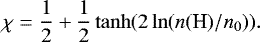
SOC was also used to calculate predictions of the 353 GHz polarised dust emission in the form of Stokes (I, Q, U) maps. This was done assuming a constant grain alignment efficiency throughout the model volume and a theoretical maximum polarisation fraction of p = 20%. The polarisation fraction is defined as
 (1)
(1)
Although we do not include noise in the polarisation simulations, we used the modified asymptotic estimator of Plaszczynski et al. (2014),
 (2)
(2)


where σQ and σU are the error estimates of Q and U and σQU their covariance. In Eq. (3) ψ0 is the true polarisation angle that is in practice replaced by its estimate
 (7)
(7)
Apart from grain alignment efficiency, here assumed to be constant, the polarisation fraction depends on the magnetic field geometry. For a single LOS, the main factors are the angle γ between the plane-of-the-sky (POS) and the B-field direction and the variations of the POS-projected magnetic field direction along the LOS. Because Q and U are proportional to cos2γ, we characterise the first factor with the averaged quantity
 (8)
(8)
where R(r) is the polarisation reduction factor, jν the dust emissivity at the observed wavelength, l is distance, and the integration extends over the full LOS (Chen et al. 2016). This quantity is independent of the field geometry projected onto the POS and, since R is kept constant, is directly the emission-weighted average of cos2γ. The observed polarisation is largest when the magnetic field is in the POS and thus when γ is zero and cos2γ is one. We denote with ⟨γ⟩ the angle that corresponds to the ⟨cos2γ⟩ value obtained from Eq. (8).
The second factor is the variation of the POS-projected magnetic field orientation along the LOS, which causes cancellation in the LOS Q and U integrals and thus leads to depolarisation. The effect can be described using the polarisation angle dispersion function
 (9)
(9)
where the summation extends over all cells along the LOS, Ψ is the local polarisation angle (i.e. for a single cell), and  is the similarly emission-weighted average angle.
The quantity SLOS only depends on data along a single LOS and is thus different from the polarisation angle dispersion function SPOS that can be derived from polarisation observations and describes variations over the sky (Planck Collaboration Int. XIX 2015). This can be calculated as
 (10)
(10)
where δ defines a spatial offset and the summation goes over N map pixels within distances [δ∕2, 3δ∕2] from the central position  . We evaluate SLOS from the synthetic observations by setting δ equal to FWHM/2 = 2.5′. The average SPOS value inside a 10′ radius circle is used to characterise the dispersion associated to a clump.
2.3 Clump catalogue
The surface brightness maps at wavelengths 100– 850 μm were analysed to extract cold clumps using a procedure that closely follows that of the PGCC study (Planck Collaboration XXVIII 2016). In the following we describe the method in detail.
The 100 μm map is compared in turn with each of the Planck maps. At the location of each pixel, the average local colour of the dust emission C = IPlanck∕I(100 μm) is estimated as the median over an annulus covering distances 5–15′ from the centre position. A map of cold residual emission is calculated as Planck band  , which differs from zero only because of local variations in the dust SED. Based on this map, the noise σCR of the cold residual is estimated as the median absolute deviation of the pixel values within an annulus from 5′ to 30′ from the centre. The background level
  is estimated as the median over the same pixels. Together these result in signal-to-noise (S/N) maps of the cold residual,
 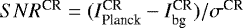 , one for each of the three Planck bands. Source candidates are identified in these maps as local maxima with SNRCR > 4, further requiring that the value is the maximum within a radius of 2′. The final merged catalogue contains sources where each of the three bands has a source candidate and the distances between the candidates are below 5′.
The second part of the clump analysis concerns the source fluxes. The 350 μm (857 GHz) source is fitted with a 2D Gaussian plus a third order polynomial background model. The fit uses the position of the detected source and returns estimates for its position angle and FWHM sizes along its major and minor axis directions. These parameters are used to separate a cold component in the 100 μm emission. A 2D Gaussian fit is appliedto the 100 μm surface brightness map using the previously fixed position and shape of the Gaussian. If there are other sources within a radius of 10′, these are fitted together as additional 2D Gaussian components (up to three Gaussians). After the fits, a corrected 100 μm warm template map is obtained by subtracting the fitted Gaussians and this is used to calculate new cold residual maps  at the threePlanck wavelengths. The flux densities of the detected clumps are estimated from these
  maps with aperture photometry. In normalised distance units r = x∕FWHMx, the aperture extends to a distance of r = 2.0. The fluxes are estimated after subtracting the local background that is calculated as the median over an annulus that extends over the distance range r = 2.0–2.5. If a source has a truly Gaussian shape, this results in flux estimates that are some 70% of the total intensity of the Gaussian.
The remaining clump characteristics are calculated based on the parameters derived above, based on synthetic observations, without resorting to direct information about the density and temperature values of the models. The source temperatures are estimated by fitting the spectral energy distribution (SED) with a modified blackbody function,
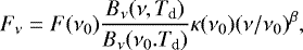 (11)
(11)
using the flux density F(ν0) at a reference frequency ν0 and the dust temperature Td as free parameters. Following the example of Planck Collaboration XXVIII (2016), we use dust opacities 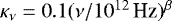 cm2 g−1 (Beckwith et al. 1990) and fix the spectral index to β = 2.0. The actual spectral index of the employed dust model is β ~ 1.84 over the 100–850 μm wavelength range. This means that the SED fit will underestimate the dust temperature but only by a fraction of one degree. Because distances d are known for all of synthetic clumps, their masses can be calculated as
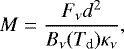 (12)
(12)
where Bν is the Planck function andTd the colour temperatureobtained from the SED fit. The aperture size and the measured flux density provide estimates of the average column density of each clump. The fitted 100 μm background component and the values of the reference annuli used in the Planck photometry provide the spectrum of the local warm background, which is used to estimate the colour temperature and the column density of the warm background.
Our procedures followed closely the methods used in Planck Collaboration XXVIII (2016), with only minor modifications. We fitted the cold residuals with a Gaussian (or up to three Gaussians), as in the case of the PGCC catalogue. However, the background was always modelled with a third order polynomial while in Planck Collaboration XXVIII (2016) the degree ranged from three to six. This can be justified by the smaller line-of-sight confusion of the synthetic observations, especially when compared to Planck observations of low Galactic latitudes.
3 Results
3.1 Clump catalogue
The total number of extracted clumps over all snapshots, view directions, and distances is of the order of 1.5 million (example shown in Fig. 1). In the following we concentrate on sources with good photometry (S/N above one) in all the four bands, which corresponds to the criterion FLUX_QUALITY=1 in the PGCC (Planck Collaboration XXVIII 2016). Figure 2 shows the number of clumps as a function of distance. At the distance of d = 100 pc, there are about 200 000 clumps per view direction, which corresponds to some 11 000 clumps per a single map (one snapshot and view direction).
Figure 3 shows clump parameters for the snapshot 377, view direction x, and the distance of d = 231 pc. The simulated clumps are compared to the PGCC sources that are to within 50% at the same distance. Both samples are limited to sources with reliable photometry (in PGCC FLUX_QUALITY=1). The FWHM sizes correspond to the Gaussian fits. The linear sizes in pc are based on the angular sizes and the known or, in the case of PGCC, estimated distances.
At the shown distance, the synthetic maps provide a few times more detections than the PGCC catalogue limited to similar distances within ± 50%. Many clump parameters are comparable between the PGCC and the synthetic catalogues. The minor axis sizes have almost identical distributions, as a direct consequence of the common threshold set by the beam size. The major axis angular sizes tend to be smaller for the synthetic clumps but this is less clear for the physical sizes since the PGCC distribution corresponds to a wider distance interval. The clump sizes are similar for all view directions and thus independent of the mean magnetic-field direction.
The largest discrepancy is in the flux densities that are about a factor of four times lower for synthetic clumps. This is reflected also in the estimates of the column densities, masses, and volume densities. On the other hand, the temperature distributions are very similar. The clump temperatures are based on the cold residual, not the total dust emission, and the separation may contribute to the similarity of the results. The background temperatures are also similar, although the synthetic observations show a narrow distribution because all models were subjected to the same radiation field.
Figure 4 shows the distributions of clump temperatures, column densities, and masses as a function of distance. This combines the statistics from all MHD snapshots and view directions. The values from the PGCC catalogue with a similar distance binning are shown for comparison.
Figure 3 indicated that the model clump temperatures are very similar to the PGCC values. Figure 4a shows that this holds for all distances d and that the average temperatures do not depend on the distance. This is somewhat unexpected given the two orders of magnitude difference in the probed linear scales. However, the PGCC shows a similar behaviour and only a marginal increase in the clump and background temperatures at the largest distances (typically sources in the inner Galaxy). In the simulations, this result could be expected because the radiation field and thus the physical dust temperatures do not vary with distance.
Figure 4b again shows the difference in the column densities. The synthetic clumps have lower values but, as in the case of the PGCC, there is a marginal increase at the largest distances. The mass estimates are very strongly connected to the resolution of the observations and scale as distance squared for both the PGCC and synthetic observations.
In the MHD simulations the turbulence is not isotropic because the magnetic field has a non-zero mean component along the y axis. Figure 5 shows observations for the three view direction, but does not indicate any significant dependence between the view direction and any of the clump properties. Similarly, Fig. 6 shows that the clump properties do not show time dependence, apart from a very minor increase of the average column density.
Figure 7 shows median intensity profiles around the extracted clumps. Clumps are divided into nine samples according tothe distance and view direction. There are further two sub-samples according to the surface brightness at the clump centre. The FWHM clump sizes tend to be only slightly larger than the beam. However, those parameters correspond to the cold emission component while the total intensity, as shown by Fig. 7 is more extended. All clumps detected in the cold residual emission are not necessarily local maxima of total surface brightness, and the profiles in Fig. 7 thus characterise more the general mass distribution in the clump environment than the intensity profile of the clumps themselves. Figure 7 includes only clumps with reliable flux measurements (S/N above two), for which the difference between the aperture and reference annulus is by definition positive.
The median profiles of the total intensity are tentatively fitted with functions
![\begin{equation*} I(r) = I_0 \left[ 1 + (r/R)^2\right]^{-\alpha} + I_{\textrm{bg}}.\end{equation*}](/articles/aa/full_html/2019/09/aa35882-19/aa35882-19-eq21.png) (13)
(13)
The parameter values α tend to be below α = 1.0 for the brighter clumps, which means that the mean intensity falls off very slowly, ~ r−0.5. The fits to lower-intensity clumps are more uncertain and for many low-intensity clumps the background level even increase at large angular distances. Such profiles cannot be well fitted with Eq. (13) and the fit parameters are not shown.
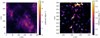 |
Fig. 1 Example of surface brightness data and clump extraction. Left frame: 850 μm map of one snapshot (number 377), with the view direction x and assumeddistance of d = 351 pc. Right frame:cold residual at 350 μm (857 GHz) for the area indicated with the dashed box in the first frame. The cyan ellipses correspond to the clumps that have been detected with S/N above four at all three Planck wavelengths and have reliable photometry in those bands and at 100 μm. |
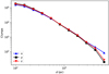 |
Fig. 2 Number of extracted clumps as a function of cloud distance. The curves correspond to the three different view directions and show the total number of clumps in the 18 snapshots. |
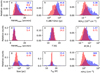 |
Fig. 3 Normalised parameter distributions for clumps in snapshot 377, direction x and distance 231 pc (red histograms). The blue histograms show the corresponding distributions for PGCC sources with within 50% the same distance. The mean values of the parameters are shown for the PGCC catalogue (upper numbers in blue) and for the simulated catalogue (lower numbers in red). The first frame also shows the number of clumps included in the plots. |
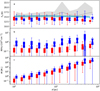 |
Fig. 4 Comparison of clump temperature, column density, and mass as functions of cloud distance. The red boxplots correspond to the simulated sample and the blue boxplots to the PGCC. Frame a: the grey shading and the cyan shading indicate theinterquartile intervals of the background temperature in the PGCC and in simulations, respectively. The median values are drawn with solid lines. |
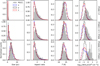 |
Fig. 5 Comparison of synthetic clump parameters for three distance intervals and view directions. The rows correspond to d < 400 pc, 400 pc < d < 1300 pc, and 1300 pc < d < 3000 pc. The columns show the distributions of physical clump size, aspect ratio, colour temperature, and column density. The data for the different view directions are shown in different colours. The corresponding data from the PGCC are plotted as grey histograms. |
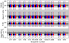 |
Fig. 6 Distributions of clump FWHM, aspect ratio, temperature, and column density as functions of MHD snapshot for clumps d < 400 pc. The boxplots correspond to data for different snapshots and directions (black, blue, and red for the x, y, and z directions, respectively). In each frame, the shaded regions correspond to the distribution of the PGCC catalogue values, light grey for the 1–99% interval and dark grey for the 25–75% interval of the cumulative probability distribution. |
3.2 Polarisation fraction in basic models
In this section we examine the polarisation fraction p of the clumps and the correlation between p and total intensity. Section 3.2.1 concentrates on the analysis of the synthetic observations and Sect. 3.2.2 looks at the correlations between p and the magnetic field structure.
3.2.1 Synthetic polarisation observations
Figure 8 shows median polarisation fraction profiles, similar to the intensity profiles of Fig. 7. In the simulations the maximum theoretical polarisation fraction was scaled to p = 20%. The values observed from the models are typically below 10%, especially in the dense regions associated with clump detections. For the view directions x and z, the polarisation fraction tends to decrease towards the clump positions. The drop is of the order of Δp = 1% and slightly more pronounced at larger distances. The clumps are divided into two sub-samples using the median value of the total intensity at the centre of the clumps. Compared to the low-intensity clumps, the median polarisation fraction of the high-intensity clumps is lower by Δp =1–2%. This applies to the x and z view directions and all radial points, which means that this a property of the clump environment rather than of the clump itself. Clumps thus reside in dense regions where p is already significantly below the average over the entire model.
The behaviour is quite different for the y direction where we observe the cloud along the mean magnetic field direction. In this case, the polarisation signal is much weaker (in the figure the values are multiplied by a factor of four) and there is no clear difference in the p of the low-intensity and high-intensity clumps. For the direction y, p tends to increase rather than decrease towards the clump centre. The behaviour is qualitatively consistent with the idea of dense clumps locally perturbing the orientation of the large-scale field, which would otherwise be parallel to the LOS.
The data from Figs. 8a–c are shown again in Fig. 9, now plotting p against the surface brightness Iν. The plot makes use of the azimuthal p and Iν averages calculated up to a distance of 40′ of the centre of each clump. For the directions x and z, the decrease in p between the lowest and highest surface brightness areas is Δp ~ 5% and thus almost a factor of two. For the direction y (along the mean-field direction) the distribution is flatter and p increases slightly towards both ends of the intensity axis. The p peak at the clump centre, as seen in Fig. 8b, is here stretched over intensities 2.5– 10 MJy sr−1.
Each frame of Fig. 8 covers a heterogeneous set of sources. Therefore, for the sources from Figs. 8a,c we correlated p with a number of other parameters, including the background intensity, S/N of the detection, and the clump size, shape, and temperature. For each clump, we also characterise the radial change of p with Δp, the difference between the mean values at 0–4′ and 10– 16′ radial distances. A negative value of Δp thus indicates a decrease of p towards the clump centre.
Figure 10 shows kernel density estimates of distributions when each parameter is plotted against Δp. The overall correlations are weak with the absolute values of the linear correlation coefficients r below 0.2. The figure includes formal probabilities ξ for Pearson correlation coefficients to be consistent with zero. Because of the set of correlated snapshots, the probabilities could be biased and we therefore quote ξ values that are calculated for a factor of 100 smaller random clump samples. For example, the comparison of Δp and the corresponding intensity contrast (the ratio of total 353 GHz surface brightness at θ <4′ divided by the average value at distances θ = 10–16′) gives r = −0.026; brighter clumps tend to havelower values of p. The correlation coefficient is small but its significance is still high. Negative correlations with Δp are observed also for the detection S/N, source flux, source column density, and the background in the cold residual map. The correlation is positive for the clump and background temperatures. Clumps with very large aspect ratios (possible filamentary morphologies) cluster around Δp = 0.
Figure 11 shows the corresponding correlations when Δp is replaced with the absolute value of the polarisation fraction at the clump centre. This results in larger correlation coefficients, which all retain the same sign as in Fig. 10. The only exception is the detection S/N, for which the correlation is now positive but with a smaller significance. Unlike in Fig. 10, the differences between the y vs. x and z directions are clear.
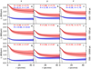 |
Fig. 7 Overview of 850 μm (353 GHz) intensity profiles of extracted clumps, divided according to view direction (columns) and distance (rows). Clumps with the central intensity above (red curves) and below (blue curves) the median intensity are plotted separately. The values are total intensities without background subtraction, normalised to the sample median value at the centre. The shaded regions correspond to the inter-quartile range. The median profiles are shown as dotted lines with the parameters R and α (see text) quoted in the frames. The Gaussians corresponding to the FWHM =5.0′ beam and the median major axis FWHM of the extracted clumps (cold component) are plotted with solid and dashed grey lines, respectively. |
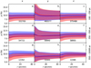 |
Fig. 8 Radial profiles of median polarisation fraction p. The clump sample is the same as in Fig. 7. The red and blue colours correspond to clumps with the central surface brightness respectively above or below the median value. The shaded regions show the inter-quartile ranges. The total number of clumps is indicated in each frame. The y-direction p values have been multiplied by a factor of four in the plot. |
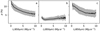 |
Fig. 9 Polarisation fraction p as a function of surface brightness for clumps in Figs. 7a–c. The clump distances are d ≤ 231 pc and the frames correspond to the view directions x, y, and z, respectively.The shading indicates the inter-quartile range. |
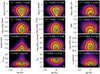 |
Fig. 10 Correlations between various parameters and Δp, the drop in polarisation towards centre of d ≤ 231 pc clumps (see text). The colour images show logarithmic point density for the clumps from Figs. 8a–c. The frames quote the linear correlation coefficients r. Probabilities ξ for r to be consistent with zero are computed for a factor of 100 smaller random clump samples. The black contours show the distribution for the combination of view directions x and z and the grey contours for the direction y. The contours are at 0.01, 0.1, 0.5, and 0.9 times the peak value. If not otherwise specified, the intensities and flux densities are the 850 μm values. |
3.2.2 Comparison to magnetic field structure
The observed polarisation fraction variations are affected by the magnetic field structure that can be characterised with ⟨ γ ⟩, SLOS, and SPOS (Eqs. (8)–(10)). Before discussing the statistics, we show in Fig. 12 ten randomly selected clumps. There is great variety in the type of p profiles, polarisation sometimes increasing rather than decreasing towards the clump centre. This small sample already suggests that p depends on both ⟨ γ ⟩ and SLOS.
Figure 13 correlates the quantities for the full sample of clumps at d = 100–231 pc. Here p, Iν, ⟨γ⟩ and SLOS are estimated towards the centre of theclumps while SPOS are averages within 10′ of the clump centre.
The correlation coefficients show that p is mostly dependent on SLOS, ⟨γ⟩, and SPOS, in that order. All correlations are highly significant and especially the dependence on SLOS is very strong with r = −0.96. The formal probabilities for r to be consistent with zero are far below 1%. The parameters ⟨γ⟩, SLOS, and SPOS show positive correlations also between themselves, with the strongest one, r = 0.73, between ⟨γ⟩ and SLOS.
Some distributions of Fig. 13 show two maxima that are related to the different view directions. The direction y, being parallel to the mean magnetic field orientation, is associated with large ⟨ γ ⟩ and low p values. The importance of this effect is illustrated further in Fig. 14, where we plot the histograms of ⟨γ⟩, SLOS, and SPOS for the differentview directions.
Appendix A includes figures similar to Fig. 13 where the y direction and the combinationof the x and y directions are shown separately. While SLOS always shows the largest negative correlation with p, its importance is somewhat reduced when the line of sight is parallel to the mean field. Similarly, the correlations between ⟨ γ ⟩, SLOS, and SPOS are lower for a given view direction. This is expected because the sub-samples (x and z directions vs. the y direction) and internally more homogeneous. For the y direction the parameters ⟨γ⟩ and SPOS become uncorrelated, although ⟨γ⟩ has significant correlation with SLOS, which is even more correlated with SPOS. Plots comparing polarisation data for different distances can also be found in Appendix A.
3.3 Modified models
We examined four modified versions of the synthetic observations. These included (1) longer lines of sight, (2) modification of the dust properties, (3) larger measurement noise, and (4) the inclusion of point sources that increase radiation field variations within the model volume (Table 1).
3.3.1 Models with longer LOS
A longer effective LOS L was obtained by adding together two or more of the original surface brightness maps. Each sum contains two, three, or four maps that thus correspond to L =2, 3, or 4 times longer LOS. For each L, we made three sets of maps using different snapshots and view directions. For example, L = 2 used combinations 377x+424y, 443y+472z, and 491z+571x, where the numbers refer to the snapshots and the letters to the view directions. For L = 3, each new map is the sum of three maps, all from different snapshots and view directions. Finally, the L = 4 maps are the sum of four maps that thus contains the same direction (x, y, or z) twice. Although these originate in different snapshots, the latter was transposed before the summation to avoid undue correlations between the component maps. For each L, in total exactly one third of the input maps is for the y direction.
Longer LOS reduces the number of clump detections (Fig. 15) but the fluxes of the extracted sources are higher and increase with L (Fig. 16). For the polarisation fraction profiles, the net effect of longer LOS is a Δp ~ 1% reduction inthe polarisation fraction (Fig. 17), which tends to increase with increasing L (not shown). The relationof p vs. surface brightness also becomes flatter but this is mainly the effect of the increased intensity values.
Figure 18 compares p to surface brightness and polarisation angle dispersion function SPOS. The absolute surface brightness is obviously correlated with L. Because of the mixing of different view directions x, y, and z into single maps, the p distribution shows here only a single peak that is between the cases of LOS being either parallel or perpendicular to the mean field. More interestingly, the differences in SPOS distributions remain small and longer LOS even shows a slight preferences for lower SPOS.
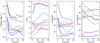 |
Fig. 12 Examples of radial profiles of Iν(850 μm), p, ⟨cos2γ⟩, and SLOS. The ten sources are selected randomly from the clumps in the snapshot 377, direction x, distance 152 pc, and S/N > 15. |
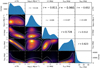 |
Fig. 13 Correlations between parameters p, Iν, ⟨γ⟩, SLOS, and SPOS. The values are estimated towards the centres of clumps at distances d ≤ 231 pc. The correlations are shown in the frames below the diagonal and the histograms of the individualparameters on the diagonal. The upper frames show the linear correlation coefficient r. The contours show separately the distributions for the combination of x and z view directions, with contours at 0.01, 0.1, 0.5, and 0.9 times the maximum probability. |
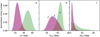 |
Fig. 14 Histograms ⟨γ⟩, SLOS, and SPOS for clumps at d = 100–231 pc. The colours blue, green, and red correspond to the view directions x, y, and z, respectively. |
Alternative models.
3.3.2 Dust properties
Alternative models were created also by changing the dust properties. Only snapshots 377, 406, 444, and 528 were used in these tests.
We consider a second dust component where the ratio of sub-millimetre and NIR dust opacities is τ(250 μ)∕τ(J) = 1.6 × 10⁻³, as derived from the statistical study of the PGCC fields observed with Herschel (Juvela et al. 2015a). This is a factor of 3.2increase of dust opacity compared to the default dust model and this relative rise was applied to λ > 30 μm. The abundance of this second dust component is
 (14)
(14)
The sum of the default and the modified dust components was kept constant. Therefore, at low densities the dust properties are as in the default model and the increased-opacity dust is limited to regions with high densities. We tested the threshold values of n0 = 1000 cm−3 and n0 = 5000 cm−3 and refer to these models as M1 and M5, respectively.
Figure 16 shows that in the modified dust case the clumps tend to have higher S/N and lower temperatures. The temperature drop is particularly clear for the higher density threshold (models M5) where the median value is close to Td = 12 K. The background intensities of M5 clumps are also much higher while the fluxes of the clumps themselves are even slightly lower. The opacity increase is thus not solving the difference to the higher PGCC source fluxes. The density threshold should affect the size of the clumps, at least if it corresponds to a volume with the size close to the original size of the extracted sources. The higher threshold of n(H) = 5000 cm−3 indeed leads to smaller clumps but the lower threshold of n(H) = 1000 cm−3 has no appreciable effect. The possible explanations are discussed in Sect. 4.3.
Figure 17a shows that the M5 clumps tend to have a high surface brightness. This means that the low flux densities result from the smaller size of the clumps. Model M5 clumps also tend to show lower polarisation but with similar shape of the radial profiles as the default models. Compared to M5, the changes in M1 are in the same direction but much less pronounced. This is interesting given that in M1 the dust property changes extend over larger areas. More than modifying the properties of individual clumps, the dust changes influence which clumps are detected.
The effect of dust properties on the observed polarisation can be seen also in Fig. 19. The distribution of p is more skewed towards small p values and the distribution of SLOS is correspondingly skewed towards larger angle dispersion values.
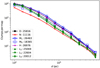 |
Fig. 15 Number of clumps per map for alternative models. The legend includes the average number of detected clumps per snapshot and direction, as the sum over all distances. |
3.3.3 Increased noise
We tested the effects of noise using the same set of snapshots as in Sect. 3.3.2. The noise of the surface brightness maps (see Sect. 2.2) was increased by a factor of five. Higher noise reduces the number of clump detections by almost the same factor (Fig. 15) and increases especially the dispersion of the clump temperature estimates. The noise also reduces the flux estimates of the clumps (the cold component) (Fig. 16). Figure 17 shows that the noise has increased the clump polarisation on average by Δp ~ 1%. Because the polarisation fraction was calculated from data without any added noise, this is not caused by bias in the p values but is a result of changes in the clump detection.
3.3.4 Radiation field variations
In the final set of alternative models, we added heating sources inside the model volume. This was done not to simulate protostellar cores, but to induce variations in the radiation field intensity and to investigate the effects that the resulting variations of the background temperature have on clump extraction. After all, according to Fig. 3h, one of the main differences compared to the PGCC catalogue is the uniformity of the colour temperature in the clump background. One hundred point sources were added to each of the four selected snapshots (377, 406, 444, and 528). The positions of the sources were selected randomly with uniform probability over the model volume. The sources were described as T = 20 000 K black bodies, with luminosities sampled from a normal distribution N(1000 L⊙, 300 L⊙). The luminosities are high enough to increase even the long-wavelength surface brightness by tens of per cent over projected distances of the order of 10 pc. Figure 20 shows the changes in dust colour temperature.
Although the effect of the heating sources is clear in the appearance of the temperature maps, it still affects significantly only a small fraction of the map areas. The effects on the parameters of the extracted clumps remain small (Fig. 16). The same applies to polarisation quantities where the changes with respect to the default model D are smaller than for the alternative dust models M5, with only a marginal widening of the p distribution (Fig. 19). The p distribution has a stronger peak at small values but the other parameters do not shown significant changes.
4 Discussion
We used radiative transfer modelling and cold-source detection methods to study the properties of dense clumps in MHD simulations of molecular clouds. The results were compared to the PGCC catalogue (Planck Collaboration XXVIII 2016). Below we discuss the clump extraction, the clump characteristics, and the relationships between the clump polarisation and the model clouds.
4.1 Clump detection
The detection and source analysis methods followed the example of the PGCC catalogue (Planck Collaboration XXVIII 2016). The detection method itself was already characterised in Montier et al. (2010) and in Planck Collaboration XXIII (2011). Because the sources are extracted from the cold residual maps, their temperature should be significantly lower than the temperatureof their environment. The main physical explanation for lower-than-average temperatures is high column density that reduces the local radiation field. This is particularly true in our simulations that do not include YSOs that could heat the clumps from inside. Nearby hot sources could lead to false detections by biasing the background temperature estimates. This necessitated the implementation of further safeguards in the analysis of the real observations (Planck Collaboration XXVIII 2016) but does not impact our simulations (without embedded sources).
At the closest distances the number of extracted clumps was of the order of 10 000 per map (Figs. 2, 15), similar to the number of sources in the PGCC catalogue. Although the models cover only a (250 pc)3 volume, this is reasonable because they represent relatively dense ISM (⟨n(H2)⟩ = 5 cm−3) and the number of resolution elements in synthetic maps is up to 50% of that in the Planck all-sky map. However, while in the PGCC only half of the detections had reliable fluxes, in the synthetic observations the corresponding fraction is over 90%. This is partly due to the absence of internal sources. Our synthetic observations also suffer less from LOS confusion, especially when compared to the PGCC where most detections are near the Galactic plane.
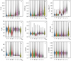 |
Fig. 16 Comparison of parameters for alternative models. Each frame shows parameter distributions for the models (see Table 1) and for the PGCC. The distributions are plotted using kernel density estimates (“violin plots”) with the quartile points indicated with horizontal lines. Frames a–i: clump 850 μm flux density, 850 μm flux density in the cold residual map, 100 μm background intensity, clump temperature, physical size, and aspect ratio, detection S/N, and the intensity and polarisation fraction contrasts (calculated as ratios of the mean values at radiae R < 4 ′ and R =10′–16′). Model results are for the distance of d = 231 pc. The PGCC distributions are plotted for selected quantities, for clumps with FLUX_QUALITY=1 and distance estimates within a factor of 1.5 of the nominal distance. |
4.2 Clump parameters in the default models
Most clump properties were similar to those in the PGCC catalogue. The almost identical distributions of minor axis FWHM reflect the cut-off set by the beam size. The major axis FWHM values are comparable although, in the basic models, the synthetic clumps tend to be smaller (Figs. 3, 5, 6). The size distribution of the PGCC is wider (Fig. 3) also because they include a range of estimated distances and the estimates have ~30% uncertainty (Planck Collaboration XXVIII 2016; Montillaud et al. 2015).
For the default models, the most noticeable difference between synthetic and PGCC clumps is in the flux densities. In Fig. 3, the PGCC clumps are on average about four times brighter and this difference is carried over to column density, mass, and volume density.
The clump temperatures are slightly higher than in the PGCC, but this finding of course depends on the assumed radiation field and the dust model. We simulated only the large-grain emission but the contribution to the 100 μm band from stochastically heated very small grains (VSGs) should get mostly eliminated when the warm-emission component is subtracted. If VSG emission caused limb brightening in the real PGCC clumps, their cold residual emission would be estimated to be smaller in their outer parts, thus leading to smaller clump sizes and flux densities. This is contrary to our finding that the synthetic clumps tended to be smaller.
4.3 Alternative cloud models
The default dust model was consistent with diffuse regions (Sect. 2.2), with τ(250 μ)∕AJ = 0.45 × 10⁻³ but dust opacity is known to be higher in molecular clouds (Planck Collaboration XXV 2011; Planck Collaboration XI 2014) and especially in dense cores (Stepnik et al. 2003; Roy et al. 2013). Therefore, we tested cases where the long-wavelength dust opacity was in dense regions increased to τ(250 μ)∕AJ = 1.6 × 10⁻³. This value was derived from Herschel observations of cloud cores and could be considered an upper limit for PGCC-type larger objects (Juvela et al. 2015a).
It would be tempting to interpret the difference between the simulated and PGCC flux densities as proof of increased sub-millimetre opacity. However, keeping the radiation field fixed, higher sub-millimetre opacities did not translate into higher source fluxes. When the long-wavelength opacity was increased, the dust temperatures decreased. For the model M5, the drop was about 2 K (Fig. 16d), almost compensating for the higher opacity. The size of the extracted clumps in M5 also decreased by almost a factor of two (Fig. 16e). The alternative density threshold n(H) = 1000 cm−3 resulted in much smaller changes. Although source fluxes might be increased by fine tuning the density threshold, it seems unlikely that the flux differences can be explained by dust properties. Conversely, our simulations do not exclude the possibility of the PGCC clumps having increased sub-millimetre opacity. One needs comparisons with other column density tracers, such as near-infrared extinction, to get direct constraints on the dust opacity (Martin et al. 2012; Roy et al. 2013; Juvela et al. 2015a).
For models L with longer LOS, the background intensities are naturally higher. However, also the clump flux densities are strongly correlated with the LOS length (Fig. 16a). This is due to the higher column densities and partly due to the increased size of the extracted clumps. In the case of L = 3–4, the flux densities are comparable to the PGCC values. With the Planck 353 GHz optical depth map at 1° resolution and the assumption of dust opacity τ(353 GHz) = 6 × 10⁻²⁷ NH (Planck Collaboration XI 2014), we estimate that the median column density at the PGCC source positions is N(H) = 8.3 × 1021 cm−2 (N(H) = 6.9 × 1021 cm−2 for the FLUX_QUALITY=1 sub-sample). This is more than twice the column density of our default model and thus in qualitative agreement with the finding that models with higher column densities are in better agreement with the PGCC observations.
If the PGCC clumps are real compact 3D objects, their observed properties should ideally be independent of the LOS length. However, we find the properties to be affected by other LOS emission. A longer LOS increases the average signal, which results in larger structures with higher integrated flux densities appearing above the noise. This is not a major factor in our simulations where the effect of L on the clump size is less than 20%. A longer LOS also means more confusion noise that leaves many of the fainter sources below the detection limit. Figure 15 indeed show that as the LOS is increased from L = 1 to L = 4, the number of sources decreases by one third. The confusion noise and the resulting selection effects thus explain the Fν vs. L correlation.
Although the observed PGCC properties are affected by projection effects, the detections algorithm itself makes use of the signature of cold dust emission. This sets preference to objects with large optical depths (also in directions perpendicular to the LOS) and thus with large volume densities. LOS confusion is likely to be a more important for continuum catalogues where the detections are based only on source brightness, without further physical constraints. The problem could be alleviated only by using radial velocity information from line measurements to identify and even separate objects along the LOS.
Increased observational noise reduced the number of detections (Fig. 15) and, unlike longer LOS, decreased the average size of the extracted clumps (Fig. 16e). In tests involving discrete heating sources, effects were seen mainly in diffuse regions (Fig. 20), with no major consequences for the clump statistics. We emphasise that these tests were concerned with variations in the radiation field external to the clumps, not the effect of protostellar sources embedded in the clumps. That would require simulations with higher spatial resolution and more careful source modelling (Malinen et al. 2011).
The separation of cold clumps from their warmer envelopes is not straightforward and requires observations in a wide wavelength range, preferably at a high spatial resolution. In real observations, this also applies to the small-grain emission, which may have some effect via its contribution to the 100 μm band and could be traced with additional shorter-wavelength bands. Similarly, the cold-clump emission can be contaminated by embedded hot sources, which should be quantified with further mid-infrared observations. Strongly heated clumps should of course not be detected as cold sources but they may affect the detectability and estimated properties of even nearby clumps (Planck Collaboration XXVIII 2016).
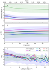 |
Fig. 17 Radial profiles and correlation between polarisation fraction and surface brightness for alternative models with d = 231 pc, as indicated in the last frame. The shaded regions correspond to the inter-quartile intervals for the models L3 (green) and M5 (blue). Frames a and b: additional curves for a S/N > 10, Td < 13 K sub-sample of the default case (dashed black lines). In frame b, these are on top of each other. Frame c: curves for the default and H cases also overlap. |
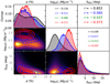 |
Fig. 18 Comparison of p, clump 850 μm intensity Iν, and SPOS for default model and longer LOS cases. The background images and the black histograms correspond to the default model and the blue and red histograms, respectively, to the L = 2 and L =4 models. From top to bottom: correlation coefficients are listed for the default case and the L = 2, 3, and 4 cases. The plot includes all clumps at d ≤ 231 pc. |
4.4 Clump polarisation
In the studyof clump polarisation, grain alignment efficiency was set constant, simply scaling the maximum theoretical polarisation fraction to p = 20%. All variations observed in p are therefore caused by the geometry of the magnetic field.
The mean magnetic field was parallel to the y axis. When LOS was perpendicular to the mean field, p values of theclumps ranged from p ~ 5% to over 10%, brighter clumps having lower polarisation fractions. For LOS parallel to the mean field, p values were 3–4 times lower and uncorrelated with the clump intensity. The radial p profiles were also qualitatively different. When LOS was perpendicular to the mean field, the average p profile decreased by Δp ~1% towards the clump centre, over a distance of ~ 10′ (Fig. 8). The drop was larger for larger cloud distances where this angular scale corresponds to cloud rather than core scales. When LOS was parallel to the field, the values increased towards the centre but on average less than Δp = 1%. Although line tangling usually leads to geometrical depolarisation, when the field is initially parallel to the LOS, the twisting of magnetic field can only increase the observed polarisation. The effect was clear in simulations and should be detectable also in observations. Appendix B shows a tentative test of this but full analysis of polarisation fraction variations in the PGCC clumps will be presented in Ristorcelli et al. (in prep.).
At largescales, we observe similar anticorrelation between column density and polarisation fraction as discussed for example in Planck Collaboration Int. XX (2015) (see, Fig. A.1). Although the clump polarisation fraction is also anti-correlated with column density, its average value is not significantly different from the average over the whole projected model, p ~ 10% for the x and z view directions (cf. Fig. 8). The values are also not sensitive to the resolution of the observations (Fig. A.1).
Figure 17 showed the radial profiles of p and the general dependence between p and surface brightness. Figure 21 shows the data in a different form, looking at the p vs. Iν relations separately for the centre of the clumps and for background points selected at 30′ distance. We also plot the upper-envelope relation pmax = −10.9 log10(N(H)) + 252.0 that was (Planck Collaboration Int. XX 2015) used to fit both Planck observations and simulated data. This matches also the upper envelope of the p vs. Iν relation of our synthetic clumps. For reference we also include the relation p = 2.02 − 0.28 × 10²² N(H2) derived for the massive filament G035.39-00.33 (Juvela et al. 2018c). This was estimated for column densities N(H2) > 1022 cm−2, values almost completely beyond the range of column densities probed by our synthetic low-resolution observations.
The simulated polarisation fraction depends only on the field geometry that was characterised with ⟨γ⟩, SLOS, and SPOS. Only SPOS is available for observers because ⟨γ⟩ and SLOS depend on field geometry along the LOS. The observed p was strongly correlated with all three parameters. The correlation coefficient was largest between p and SLOS, some r = −0.96 in the case of the mixed sample of different view directions (Fig. 13). Comparison with ⟨γ⟩ gave a value of r = −0.81 and comparison with SPOS still a very significant value of r = −0.65. This is not surprising because SPOS, ⟨γ⟩ are naturally correlated: when γ is close to 90° and the magnetic field is mainly along the LOS, the angles of the B field projected onto POS will have a large scatter. This applies both to the behaviour along single LOS (SLOS) and the resulting polarisation angle dispersion on the sky (SPOS). However, while the correlations between SLOS and ⟨γ⟩ on one hand and SLOS and SPOS on the other were both strong (r > 0.6), the correlation between SPOS and ⟨γ⟩ was significantly lower (Fig. 13). It was boosted by the mixture of view directions and disappeared in observations along the mean-field direction (Fig. A.3).
The longer LOS model (Sect. 3.3.1) were associated with some decrease in SPOS. In Mangilli et al. (2019), similar effect was seen in PILOT balloon-borne telescope (Bernard et al. 2016) observations of low Galactic latitudes and interpreted as averaging over many turbulent cells, which recovers the mean Galactic field orientation. In our simulations, the effect is also strong because of the relatively uniform mean-field direction.
The alternative models (Table 1) introduced minor changes in the polarisation relations. Increased dust opacity in dense regions leads to a decrease in the p values by Δp ~1% (Fig. 17). According to Fig. 19, this is caused mainly by an increased dispersion SLOS. If this were due to the different relative weighting of LOS areas, this would imply that clumps have a more uniform magnetic field compared to the rest of the 250 pc LOS. However, there are also other factors, for example, the clump selection. Figures A.2 and A.3 show that the y direction is associated with much lower p and higher SLOS values, which leads to the almost bimodal distributions of Fig. 19. Thus, the changes (lower p, higher SLOS) can be explained by a larger fraction of y-direction clumps. The alternative dust model M5 does indeed increase the relative amount of y-direction clumps by some 6%. When the effect of modified dust is examined for each direction separately, the shapes of the p and SLOS distributions do not change for the y direction but for the x and z directions p moves towards lower values and SLOS towards higher values. This is consistent with increased dust opacity giving more weight for regions with more tangled fields. The effects in Fig. 19 thus have two causes, the larger fraction of y-direction clumps and the enhanced geometrical depolarisation.
The only noticeable effect of discrete heating sources was in the p distribution where the peak at p~ 2% is slightly stronger and the number of clumps with p > 10% is higher (Fig. 19). The relative number of clumps detected towards the three view directions is not affected. The tail towards high p is thus probably related to the increased temperature contrast, which results in the detection of more tenuous clumps with higher polarisation fractions. The heating of diffuse material increases its contribution to the polarised intensity, also contributing to the steepening of the radialp profiles of the clumps (Fig. 17).
Figure 17 showed p profiles also for the cases of increased observational noise. We emphasise that this noise applies only to the observations leading to the detection and basic characterisation of the clumps. The polarisation data were simulated without observational noise to avoid the complications biased p estimates. Higher noise level should lead to the detection of clumps with preferentially higher column densities and thus lower p. However, in Fig. 17 noise has increased the polarisation fractions at the clump centre by Δp ~ 1% (Fig. 17b). However, this again results from a change in the relative number of clumps for the different view directions. Increased noise reduced the relative number of the y-direction clumps from 35.5 to 24.1%. Because of the much lower p values of they-direction clumps, thisaffects the overall polarisation statistics.
Larger column densities provide more chances for geometrical depolarisation and the net effect on p was mostly negative also in our simulations. In Fig. 18, p decreases with L, especially on the side of high p values. Furthermore, the p values tend to decrease more outside the clumps, making the radial profiles flatter (Fig. 17). At the clump centre, the average polarisation fraction is reduced by Δp = 1%. Relative to the default models, p increases only at the highest surface brightness values (Fig. 17c), in a small fraction of all clumps. However, the effect might be detectable for the real PGCC clumps that, as discussed in Sect. 4.3, typically correspond to higher column densities. The general anticorrelation between p and N(H) is of course well known based on previous observations and simulations (Vrba et al. 1976; Gerakines et al. 1995; Ward-Thompson et al. 2000; Planck Collaboration Int. XIX 2015; Alves et al. 2014; Planck Collaboration Int. XX 2015; Planck Collaboration XII 2019; Juvela et al. 2018c; Seifried et al. 2019; Coudé et al. 2019).
Our results on polarisation fraction are qualitatively similar to the core-scale simulations of Chen et al. (2016), where strong correlations were also observed between p, ⟨γ⟩, and SLOS. Chen et al. (2016) found that, compared to field inclination effects, polarisation fraction decreases during later core evolution relatively more because of the increased field tangling. Compared to those simulations, our clumps represent both larger scales and earlier pre-stellar stages. Another difference is the contribution from the LOS, outside the main clump. Our 250 pc LOS prevents the observed p values from becoming very low even towards the densest clumps (view direction y excluded). Based on the difference in column densities, such LOS contributions should be even stronger in the case of the low-latitude PGCC clumps. Another question related to the LOS confusion is how the background affects observations from interferometers and ground-based instruments, when the extended emission is filtered out from the observations. The importance of this on the recovered field morphology is, however, outside the scope of this paper.
The comparison of these simulations and observations, especially those of the PGCC clumps, can be used to address further the questions of dust opacity and grain alignment. Figure 17a showed that the surface brightness contrast between the clump centre and the environment at 30′ distance is for the Td < 13 K sample only ~1.65. For the corresponding sample of PGCC clumps this ratio is close to two (Ristorcelli et al., in prep.). However, in our tests the modified-dust-opacity models M1 and M5 did not significantly change the contrast and it may be more sensitive to the details of the clump selection than the dust properties. For example, both noise and background fluctuations (LOS confusion) directly lead to an increase in the average brightness of the detected clumps.
The variations of dust polarisation are more interesting. The polarisation fraction p drops towards the simulated clumps on average by less than Δp = 2%. For the y direction, when LOS is parallel to the mean field, the polarisation even increases towards the clumps. For the x and z view directions, the average ratio of p values measured at the clump centre and in the background at 30′ distance is 0.85. For the PGCC, the corresponding factor is ~0.60. This is thus significantly smaller, even though the PGCC sources should correspond to a mixture of different LOS vs. B-field configurations. This suggests that the polarised emission from dense clumps is reduced by additional factors, such as the RAT mechanism.
Assuming that RAT is the main grain alignment mechanism, polarised emission should be reduced in regions with weakerradiation fields. In the PGCC and in our simulations, the sources are selected directly based on their spectral cold-dust signature, which means that their inner regions are strongly shielded from the interstellar radiation field. Because grain alignment is disturbed by collision, the other main parameter is the local density. Early numerical studies predicted clear drop of emitted polarised intensity from clumps shielded by AV of a few and densities in MHD simulations above n(H_2) ~ 103 cm−3 (Bethell et al. 2007; Pelkonen et al. 2007, 2009). With more recent molecular-cloud simulations,Seifried et al. (2019) concluded that RAT would remain effective up to densities n(H2) ~ 104 cm−3. Observations do show a strong drop in p towards dense filaments and cores (Brauer et al. 2016; Juvela et al. 2018c; Kandori et al. 2018) but in individual sources it is difficult to disentangle the effects of dust physics from those of the field geometry. According to RAT theory the polarisation fraction should drop continuously with increasing volume density. The actual effect thus depends critically on the nature of the studied objects. The PGCC contains a very heterogeneous collection of sources, from nearby cloud cores (average densities above 104 cm−3) to more distant extended cloud structures, sometimes with very high column densities (such as infrared dark clouds). Large uncertainties are still associated with the dust properties, what is the grain size distribution inside the cold clumps and how grain evolution affects the emission and the alignment (Pelkonen et al. 2009; Reissl et al. 2017). The polarisation fraction of the PGCC clumps will be investigated further in Ristorcelli et al. (in prep.). This analysis and further modelling of Planck polarisation data should shed more light on these questions.
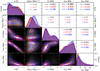 |
Fig. 19 Comparison of polarisation-related parameters for alternative models. The lower frames show kernel-density-estimated parameter correlations and the diagonal frames the histograms of individual parameters. The correlation coefficients are listed in the remaining frames. The background images and histograms drawn with black lines correspond to the default model D with all clumps d < 300 pc. The data for the alternative models H (internal heating sources) and M5 (modified dust properties) are drawn in red and blue, respectively. |
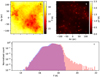 |
Fig. 20 Effect of internal sources on dust colour temperature. Frame a: temperature map for the default model D (snapshot 406, direction x) and frame b: change in the temperatures resulting in model H from 100 radiation sources inside the model volume. The temperature histograms are shown in frame c (blue for model D and red for model H). |
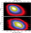 |
Fig. 21 Relations p vs. Iν for clump centres (colour images) and for background at 30′ distance (contours, in steps of 0.2 from 0.1 to 0.9 of the peak value). The plots include all clumps at d = 231 pc viewed from the x and y directions (frame a) and a subset with S/N > 10 and Td< 13 K (frame b). The dashed red line in frame b shows the upper envelope derived in Planck Collaboration Int. XX (2015). The cyan line is the relation estimated for the dense filament G035.39-00.33 (Juvela et al. 2018c) and is drawn for N(H2) > 1022 cm−2. The column density scale corresponding to Td = 15 K. |
5 Conclusions
We have used numerical simulations of interstellar clouds to make synthetic observations of a large number of cold clumps. The clumps were extracted with a detection method similar to that used for the PGCC (Planck Collaboration XXVIII 2016). We compared the properties of the simulated clumps with those of the PGCC sources. We also examined the polarisation fraction variations associated to the clumps. The study has led to the following conclusions.
Many physical clump properties (e.g. sizes, aspect ratios, and temperatures) of the simulated clumps are very similar to those in the Planck survey. However, especially the clump size distributions are determined mainly by the angular resolution of the observations and the upper limit set by the detection method.
The column densities of the synthetic clumps are lower than in the PGCC. This was concluded to be caused mainly by the model column densities that are lower than those encountered in the PGCC at low and intermediate Galactic latitudes. The observed clump column density distribution can be matched by increasing the average column density by a factor of 2–3. This suggests that the derived clump properties, also in the PGCC, are not properties of well-defined compact 3D sources but do depend on LOS confusion. The apparent difference in column densities can not be interpreted as direct evidence of increased dust sub-millimetre emissivity, although the simulations cannot exclude that possibility either.
The clumps are usually associated with a small decrease in the polarisation fraction, Δp ~ 1%, relative to their surroundings. In the more rare case, where the mean magnetic field parallel to the LOS, p tends to increase towards the clumps. This is caused by the very low background values and is typically less than Δp = 0.5%.
The alternative models show some noticeable changes in the polarisation fraction. Higher dust opacity (model M5) and increased LOS (model L3) decrease the p values towards clump centres by Δp = 1%. In the case of the latter, polarisation remains lower also outside the clumps and thus results in a low contrast in the p values between the clumps and their environment. Larger observational noise increases the average column density and decreases the average p of the extracted clumps. On the other hand, the discrete heating sources, used to increase the level and variations of the radiation field within the model volume, have but a marginal effect on the polarisation and other clump properties.
The surface brightness contrast between the clumps and their background is smaller for the simulated clumps than for the PGCC clumps. The drop in p is also smaller in the simulations, which suggests that the polarised emission from the PGCC clumps may be affected by additional factors, such as the imperfect grain alignment predicted by the RAT mechanism. This will be addressed in future studies.
Acknowledgements
M.J. acknowledges the support of the Academy of Finland Grant No. 285 769. P.P. acknowledges support by the Spanish MINECO under project AYA2017-88 754-P. V.M.P. acknowledges support by the Spanish MINECO under projects MDM-2014-0369 and AYA2017-88 754-P. We thankfully acknowledge the computer resources at MareNostrum and the technical support provided by Barcelona Supercomputing Center (AECT-2018-3-0019).
Appendix A Additional plots of polarisation quantities
Figures A.2 and A.3 show the correlations of the clump polarisation fraction p with other parameters. The figures are similar to Fig. 13 but show the data separately for the combination of x and z directions where the LOS is mainly perpendicular to the mean field direction (Fig. A.2) and for the y direction where it is mainly parallel to the field (Fig. A.3). Figure A.4 compares the same parameters for the default models at three distances, 152, 533, and 1232 pc.
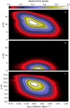 |
Fig. A.1 Polarisation fraction as function of 850 μm intensity over whole snapshot 377 (model D). The frames a–c correspond, respectively, to the view directions x, y, and z. The colour images show the distribution for the full-resolution maps and the contours (drawn in steps of 10% between 10 and 90% of the maximum value) for lower-resolution data that correspond to a distance of 351 pc. |
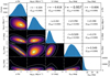 |
Fig. A.2 Same as Fig. 13 but only for clumps viewed from x and z directions. Upper right frames include probabilities ξ100 for r to be consistent with zero. These are calculated using random samples that are a factor of 100 smaller than the full clump samples. |
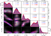 |
Fig. A.4 As Fig. 13 but comparing default models at different distances. The background images and histograms plotted with black lines are for d = 152 pc. Data for distances d = 533 pc and d = 1232 pc are drawn with blue and red lines (and contours), respectively. The correlation coefficients in the frames above the diagonal arewritten in the corresponding colours. |
Appendix B Polarisation fraction of PGCC clumps
The full analysis of polarisation fraction variations will be presented in Ristorcelli et al. (in prep.). However, we make here a preliminary test to see if the dichotomy of p profiles is detectable also for the real PGCC clumps (cf. Sect. 4.4). When LOS is perpendicular to the mean field direction, simulations showed several percent higher polarisation fractions, p decreasing towards the clump centre. When LOS was parallel to the mean field, the clumps had higher polarisation than their environment. However, these radial variations were on average less than 1%.
We calculated pmax estimates from the Planck all-sky maps and extracted radial intensity and p profiles for the PGCC clumps. This was done in a similar way as in the analysis of the simulated data (cf. Sect. 3.2.1). However, to decrease the effects of noise (present in observations but not in our simulations), the input maps were first convolved to 10′ resolution. Figure B.1 shows p as function of intensity and the estimated γ angle. This angle is calculated based on the Galactic coordinates and the distance of the PGCC clumps, assuming that Milky Way would have an ordered large-scale field. We assume that the field would be main azimuthal, with a pitch angle of 14°, as estimated for the spiral structure (Vallée 2017). The results are shown in Fig. B.1.
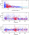 |
Fig. B.1 Polarisation fraction associated to selected PGCC clumps. The first frame shows the relation p vs. intensity when both are measured at the clump centres. The second frame shows p as a functionof the estimated γ angle. The last frame shows the same for the p contrast (p at the clumpcentre divided by the average over radial distances 16–20′). The blue and red colours correspond to two clump samples (see text). The cyan and magenta lines show the corresponding median values calculated with a moving window with the width one tenth of the data range. |
The analysis is naturally limited to clumps with distance estimates. We further limit the sample to sources with distances d < 8.5 kpc and with central intensity higher than Iν(353 GHz) = 5 MJy sr−1. These sources are plotted in Fig. B.1 in blue colour. The scatter of p values is increasing towards lower intensities. This is a sign of the estimates are becoming more uncertain and possibly biased because of the noise. We include in the plots also a more restricted set of sources. This includes only clumps with intensities above 5 MJy sr−1, with distances 200–5000 pc, and Galactic latitudes b = 2–30°. The constraint were included in an attempt to eliminate the most confused LOS in the Galactic plane and to avoid giving a high weight for the nearby clouds that may have systematic deviations from our very simple model for the γ angles. This second set of sources is plotted in red colour.
Figure B.1b is thus expected to show a decrease in p values between the perpendicular (γ = 0°) and the parallel (γ = 90°) cases. Such a negative trend is also observed, p decreasing by almost Δp = 3% as γ increases from 0° to 90°. The trend is similar for both clump samples. The trend should in principle be statistically significant because γ is not expected to be strongly correlated with clump intensity, which in turn is strongly correlated with the p uncertainties and p bias.
The angle between LOS and magnetic field has in simulations a smaller effect on the shape of the radial p profiles. In Fig. 8, the relative change between the clump centre and values at distances R >10′ is only of the order of 10%. Figure B.1c plots the contrast of p values as a function the angle γ for the PGCC clumps. The contrast is here defined as p in the clump centre divided by the mean value over distances R =16–20′. There is a marginal trend that agrees with the simulations: the contrast is smaller for small γ angles. However, the median values remain below one, even when the field is supposed to be parallel to the LOS (γ = 90°).
References
- Alina, D., Ristorcelli, I., Montier, L., et al. 2019, MNRAS, 485, 2825 [NASA ADS] [CrossRef] [Google Scholar]
- Alves, F. O., Franco, G. A. P., & Girart, J. M. 2008, A&A, 486, L13 [NASA ADS] [CrossRef] [EDP Sciences] [Google Scholar]
- Alves, F. O., Frau, P., Girart, J. M., et al. 2014, A&A, 569, L1 [NASA ADS] [CrossRef] [EDP Sciences] [Google Scholar]
- Beckwith, S. V. W., Sargent, A. I., Chini, R. S., & Guesten, R. 1990, AJ, 99, 924 [NASA ADS] [CrossRef] [Google Scholar]
- Bernard, J.-P., Ade, P., André, Y., et al. 2016, Exp. Astron., 42, 199 [NASA ADS] [CrossRef] [Google Scholar]
- Bethell, T. J., Chepurnov, A., Lazarian, A., & Kim, J. 2007, ApJ, 663, 1055 [NASA ADS] [CrossRef] [Google Scholar]
- Brauer, R., Wolf, S., & Reissl, S. 2016, A&A, 588, A129 [NASA ADS] [CrossRef] [EDP Sciences] [Google Scholar]
- Chapman, N. L., Goldsmith, P. F., Pineda, J. L., et al. 2011, ApJ, 741, 21 [NASA ADS] [CrossRef] [Google Scholar]
- Chen, C.-Y., King, P. K., & Li, Z.-Y. 2016, ApJ, 829, 84 [NASA ADS] [CrossRef] [Google Scholar]
- Cho, J., & Lazarian, A. 2005, ApJ, 631, 361 [NASA ADS] [CrossRef] [Google Scholar]
- Compiègne, M., Verstraete, L., Jones, A., et al. 2011, A&A, 525, A103 [NASA ADS] [CrossRef] [EDP Sciences] [Google Scholar]
- Coudé, S., Bastien, P., Houde, M., et al. 2019, ApJ, 877, 88 [NASA ADS] [CrossRef] [Google Scholar]
- Cox, N. L. J., Arzoumanian, D., André, P., et al. 2016, A&A, 590, A110 [NASA ADS] [CrossRef] [EDP Sciences] [Google Scholar]
- Fehér, O., Juvela, M., Lunttila, T., et al. 2017, A&A, 606, A102 [NASA ADS] [CrossRef] [EDP Sciences] [Google Scholar]
- Fissel, L. M., Ade, P. A. R., Angilé, F. E., et al. 2016, ApJ, 824, 134 [NASA ADS] [CrossRef] [Google Scholar]
- Gerakines, P. A., Whittet, D. C. B., & Lazarian, A. 1995, ApJ, 455, L171 [NASA ADS] [CrossRef] [Google Scholar]
- Goodman, A. A., Jones, T. J., Lada, E. A., & Myers, P. C. 1995, ApJ, 448, 748 [NASA ADS] [CrossRef] [Google Scholar]
- Heyer, M. H., & Terebey, S. 1998, ApJ, 502, 265 [NASA ADS] [CrossRef] [Google Scholar]
- Hoang, T., & Lazarian, A. 2014, MNRAS, 438, 680 [NASA ADS] [CrossRef] [Google Scholar]
- Juvela, M. 2019, A&A, 622, A79 [NASA ADS] [CrossRef] [EDP Sciences] [Google Scholar]
- Juvela, M., Ristorcelli, I., Pagani, L., et al. 2012, A&A, 541, A12 [NASA ADS] [CrossRef] [EDP Sciences] [Google Scholar]
- Juvela, M., Ristorcelli, I., Marshall, D. J., et al. 2015a, A&A, 584, A93 [NASA ADS] [CrossRef] [EDP Sciences] [Google Scholar]
- Juvela, M., Demyk, K., Doi, Y., et al. 2015b, A&A, 584, A94 [NASA ADS] [CrossRef] [EDP Sciences] [Google Scholar]
- Juvela, M., Malinen, J., Montillaud, J., et al. 2018a, A&A, 614, A83 [NASA ADS] [CrossRef] [EDP Sciences] [Google Scholar]
- Juvela, M., He, J., Pattle, K., et al. 2018b, A&A, 612, A71 [NASA ADS] [CrossRef] [EDP Sciences] [Google Scholar]
- Juvela, M., Guillet, V., Liu, T., et al. 2018c, A&A, 620, A26 [NASA ADS] [CrossRef] [EDP Sciences] [Google Scholar]
- Kandori, R., Tamura, M., Nagata, T., et al. 2018, ApJ, 857, 100 [NASA ADS] [CrossRef] [Google Scholar]
- Kennicutt, Jr. R. C. 1998, ApJ, 498, 541 [NASA ADS] [CrossRef] [Google Scholar]
- Koch, P. M., Tang, Y.-W., Ho, P. T. P., et al. 2014, ApJ, 797, 99 [NASA ADS] [CrossRef] [Google Scholar]
- Lazarian, A., Goodman, A. A., & Myers, P. C. 1997, ApJ, 490, 273 [NASA ADS] [CrossRef] [Google Scholar]
- Liu, T., Zhang, Q., Kim, K.-T., et al. 2016, ApJS, 222, 7 [NASA ADS] [CrossRef] [Google Scholar]
- Liu, T., Kim, K.-T., Juvela, M., et al. 2018a, ApJS, 234, 28 [NASA ADS] [CrossRef] [Google Scholar]
- Liu, T., Li, P. S., Juvela, M., et al. 2018b, ApJ, 859, 151 [NASA ADS] [CrossRef] [Google Scholar]
- Liu, T., Kim, K.-T., Liu, S.-Y., et al. 2018c, ApJ, 869, L5 [NASA ADS] [CrossRef] [Google Scholar]
- Malinen, J., Juvela, M., Collins, D. C., Lunttila, T., & Padoan, P. 2011, A&A, 530, A101 [NASA ADS] [CrossRef] [EDP Sciences] [Google Scholar]
- Malinen, J., Montier, L., Montillaud, J., et al. 2016, MNRAS, 460, 1934 [Google Scholar]
- Mangilli, A., Aumont, J., Bernard, J. P., et al. 2019, A&A, in press, http://doi.org/10.1051/0004-6361/201935072 [Google Scholar]
- Martin, P. G., Roy, A., Bontemps, S., et al. 2012, ApJ, 751, 28 [NASA ADS] [CrossRef] [Google Scholar]
- Mathis, J. S., Mezger, P. G., & Panagia, N. 1983, A&A, 128, 212 [NASA ADS] [Google Scholar]
- Matthews, T.G., Ade, P. A. R., Angilé, F. E., et al. 2014, ApJ, 784, 116 [NASA ADS] [CrossRef] [Google Scholar]
- Meng, F., Wu, Y., & Liu, T. 2013, ApJS, 209, 37 [NASA ADS] [CrossRef] [Google Scholar]
- Miville-Deschênes, M., & Lagache, G. 2005, ApJS, 157, 302 [NASA ADS] [CrossRef] [Google Scholar]
- Montier, L. A., Pelkonen, V.-M., Juvela, M., Ristorcelli, I., & Marshall, D. J. 2010, A&A, 522, A83 [NASA ADS] [CrossRef] [EDP Sciences] [Google Scholar]
- Montillaud, J., Juvela, M., Rivera-Ingraham, A., et al. 2015, A&A, 584, A92 [NASA ADS] [CrossRef] [EDP Sciences] [Google Scholar]
- Neha,S., Maheswar, G., Soam, A., & Lee, C. W. 2018, MNRAS, 476, 4442 [NASA ADS] [CrossRef] [Google Scholar]
- Neugebauer, G., Habing, H. J., van Duinen, R., et al. 1984, ApJ, 278, L1 [Google Scholar]
- Ossenkopf, V., & Henning, T. 1994, A&A, 291, 943 [NASA ADS] [Google Scholar]
- Padoan, P., Pan, L., Haugbølle, T., & Nordlund, Å. 2016a, ApJ, 822, 11 [NASA ADS] [CrossRef] [Google Scholar]
- Padoan, P., Juvela, M., Pan, L., Haugbølle, T., & Nordlund, Å. 2016b, ApJ, 826, 140 [NASA ADS] [CrossRef] [Google Scholar]
- Padoan, P., Haugbølle, T., Nordlund, Å., & Frimann, S. 2017, ApJ, 840, 48 [NASA ADS] [CrossRef] [Google Scholar]
- Parikka, A., Juvela, M., Pelkonen, V.-M., Malinen, J., & Harju, J. 2015, A&A, 577, A69 [NASA ADS] [CrossRef] [EDP Sciences] [Google Scholar]
- Pattle, K., Ward-Thompson, D., Berry, D., et al. 2017, ApJ, 846, 122 [NASA ADS] [CrossRef] [Google Scholar]
- Pelkonen, V. M., Juvela, M., & Padoan, P. 2007, A&A, 461, 551 [NASA ADS] [CrossRef] [EDP Sciences] [Google Scholar]
- Pelkonen, V.-M., Juvela, M., & Padoan, P. 2009, A&A, 502, 833 [NASA ADS] [CrossRef] [EDP Sciences] [Google Scholar]
- Pereyra, A., & Magalhães, A. M. 2004, ApJ, 603, 584 [NASA ADS] [CrossRef] [Google Scholar]
- Planck Collaboration XXII. 2011, A&A, 536, A22 [NASA ADS] [CrossRef] [EDP Sciences] [Google Scholar]
- Planck Collaboration XXIII. 2011, A&A, 536, A23 [NASA ADS] [CrossRef] [EDP Sciences] [Google Scholar]
- Planck Collaboration XXV. 2011, A&A, 536, A25 [NASA ADS] [CrossRef] [EDP Sciences] [Google Scholar]
- Planck Collaboration XI. 2014, A&A, 571, A11 [NASA ADS] [CrossRef] [EDP Sciences] [Google Scholar]
- Planck Collaboration I. 2016, A&A, 594, A1 [NASA ADS] [CrossRef] [EDP Sciences] [Google Scholar]
- Planck Collaboration X. 2016, A&A, 594, A10 [NASA ADS] [CrossRef] [EDP Sciences] [Google Scholar]
- Planck Collaboration XXVIII. 2016, A&A, 594, A28 [NASA ADS] [CrossRef] [EDP Sciences] [Google Scholar]
- Planck Collaboration XII. 2019, A&A, in press, http://doi.org/10.1051/0004-6361/201833885 [Google Scholar]
- Planck Collaboration Int. XX. 2015, A&A, 576, A105 [NASA ADS] [CrossRef] [EDP Sciences] [Google Scholar]
- Planck Collaboration Int. XIX. 2015, A&A, 576, A104 [NASA ADS] [CrossRef] [EDP Sciences] [Google Scholar]
- Planck Collaboration Int. XXXIII. 2016, A&A, 586, A136 [NASA ADS] [CrossRef] [EDP Sciences] [Google Scholar]
- Plaszczynski, S., Montier, L., Levrier, F., & Tristram, M. 2014, MNRAS, 439, 4048 [NASA ADS] [CrossRef] [Google Scholar]
- Reissl, S., Seifried, D., Wolf, S., Banerjee, R., & Klessen, R. S. 2017, A&A, 603, A71 [NASA ADS] [CrossRef] [EDP Sciences] [Google Scholar]
- Reissl, S., Stutz, A. M., Brauer, R., et al. 2018, MNRAS, 481, 2507 [NASA ADS] [CrossRef] [Google Scholar]
- Rivera-Ingraham, A., Ristorcelli, I., Juvela, M., et al. 2016, A&A, 591, A90 [NASA ADS] [CrossRef] [EDP Sciences] [Google Scholar]
- Roy, A., Martin, P. G., Polychroni, D., et al. 2013, ApJ, 763, 55 [NASA ADS] [CrossRef] [Google Scholar]
- Seifried, D., Walch, S., Reissl, S., & Ibáñez-Mejía, J. C. 2019, MNRAS, 482, 2697 [NASA ADS] [CrossRef] [Google Scholar]
- Soler, J. D., Alves, F., Boulanger, F., et al. 2016, A&A, 596, A93 [NASA ADS] [CrossRef] [EDP Sciences] [Google Scholar]
- Stepnik, B., Abergel, A., Bernard, J., et al. 2003, A&A, 398, 551 [NASA ADS] [CrossRef] [EDP Sciences] [Google Scholar]
- Tatematsu, K., Liu, T., Ohashi, S., et al. 2017, ApJS, 228, 12 [NASA ADS] [CrossRef] [Google Scholar]
- Teyssier, R. 2002, A&A, 385, 337 [NASA ADS] [CrossRef] [EDP Sciences] [Google Scholar]
- Vallée, J. P. 2017, Astron. Rev., 13, 113 [Google Scholar]
- Vrba, F. J., Strom, S. E., & Strom, K. M. 1976, AJ, 81, 958 [NASA ADS] [CrossRef] [Google Scholar]
- Ward-Thompson, D., Kirk, J. M., Crutcher, R. M., et al. 2000, ApJ, 537, L135 [NASA ADS] [CrossRef] [Google Scholar]
- Ward-Thompson, D., Pattle, K., Bastien, P., et al. 2017, ApJ, 842, 66 [NASA ADS] [CrossRef] [Google Scholar]
- Whittet, D. C. B., Gerakines, P. A., Hough, J. H., & Shenoy, S. S. 2001, ApJ, 547, 872 [NASA ADS] [CrossRef] [Google Scholar]
- Wu, Y., Liu, T., Meng, F., et al. 2012, ApJ, 756, 76 [NASA ADS] [CrossRef] [Google Scholar]
- Zhang, C.-P., Liu, T., Yuan, J., et al. 2018, ApJS, 236, 49 [NASA ADS] [CrossRef] [Google Scholar]
- Zhang, T., Wu, Y., Liu, T., & Meng, F. 2016, ApJS, 224, 43 [NASA ADS] [CrossRef] [Google Scholar]
All Tables
All Figures
|
Fig. 1 Example of surface brightness data and clump extraction. Left frame: 850 μm map of one snapshot (number 377), with the view direction x and assumeddistance of d = 351 pc. Right frame:cold residual at 350 μm (857 GHz) for the area indicated with the dashed box in the first frame. The cyan ellipses correspond to the clumps that have been detected with S/N above four at all three Planck wavelengths and have reliable photometry in those bands and at 100 μm. |
| In the text | |
|
Fig. 2 Number of extracted clumps as a function of cloud distance. The curves correspond to the three different view directions and show the total number of clumps in the 18 snapshots. |
| In the text | |
|
Fig. 3 Normalised parameter distributions for clumps in snapshot 377, direction x and distance 231 pc (red histograms). The blue histograms show the corresponding distributions for PGCC sources with within 50% the same distance. The mean values of the parameters are shown for the PGCC catalogue (upper numbers in blue) and for the simulated catalogue (lower numbers in red). The first frame also shows the number of clumps included in the plots. |
| In the text | |
|
Fig. 4 Comparison of clump temperature, column density, and mass as functions of cloud distance. The red boxplots correspond to the simulated sample and the blue boxplots to the PGCC. Frame a: the grey shading and the cyan shading indicate theinterquartile intervals of the background temperature in the PGCC and in simulations, respectively. The median values are drawn with solid lines. |
| In the text | |
|
Fig. 5 Comparison of synthetic clump parameters for three distance intervals and view directions. The rows correspond to d < 400 pc, 400 pc < d < 1300 pc, and 1300 pc < d < 3000 pc. The columns show the distributions of physical clump size, aspect ratio, colour temperature, and column density. The data for the different view directions are shown in different colours. The corresponding data from the PGCC are plotted as grey histograms. |
| In the text | |
|
Fig. 6 Distributions of clump FWHM, aspect ratio, temperature, and column density as functions of MHD snapshot for clumps d < 400 pc. The boxplots correspond to data for different snapshots and directions (black, blue, and red for the x, y, and z directions, respectively). In each frame, the shaded regions correspond to the distribution of the PGCC catalogue values, light grey for the 1–99% interval and dark grey for the 25–75% interval of the cumulative probability distribution. |
| In the text | |
|
Fig. 7 Overview of 850 μm (353 GHz) intensity profiles of extracted clumps, divided according to view direction (columns) and distance (rows). Clumps with the central intensity above (red curves) and below (blue curves) the median intensity are plotted separately. The values are total intensities without background subtraction, normalised to the sample median value at the centre. The shaded regions correspond to the inter-quartile range. The median profiles are shown as dotted lines with the parameters R and α (see text) quoted in the frames. The Gaussians corresponding to the FWHM =5.0′ beam and the median major axis FWHM of the extracted clumps (cold component) are plotted with solid and dashed grey lines, respectively. |
| In the text | |
|
Fig. 8 Radial profiles of median polarisation fraction p. The clump sample is the same as in Fig. 7. The red and blue colours correspond to clumps with the central surface brightness respectively above or below the median value. The shaded regions show the inter-quartile ranges. The total number of clumps is indicated in each frame. The y-direction p values have been multiplied by a factor of four in the plot. |
| In the text | |
|
Fig. 9 Polarisation fraction p as a function of surface brightness for clumps in Figs. 7a–c. The clump distances are d ≤ 231 pc and the frames correspond to the view directions x, y, and z, respectively.The shading indicates the inter-quartile range. |
| In the text | |
|
Fig. 10 Correlations between various parameters and Δp, the drop in polarisation towards centre of d ≤ 231 pc clumps (see text). The colour images show logarithmic point density for the clumps from Figs. 8a–c. The frames quote the linear correlation coefficients r. Probabilities ξ for r to be consistent with zero are computed for a factor of 100 smaller random clump samples. The black contours show the distribution for the combination of view directions x and z and the grey contours for the direction y. The contours are at 0.01, 0.1, 0.5, and 0.9 times the peak value. If not otherwise specified, the intensities and flux densities are the 850 μm values. |
| In the text | |
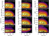 |
Fig. 11 Same as Fig. 10 but plotting quantities against p at the clump centre. |
| In the text | |
|
Fig. 12 Examples of radial profiles of Iν(850 μm), p, ⟨cos2γ⟩, and SLOS. The ten sources are selected randomly from the clumps in the snapshot 377, direction x, distance 152 pc, and S/N > 15. |
| In the text | |
|
Fig. 13 Correlations between parameters p, Iν, ⟨γ⟩, SLOS, and SPOS. The values are estimated towards the centres of clumps at distances d ≤ 231 pc. The correlations are shown in the frames below the diagonal and the histograms of the individualparameters on the diagonal. The upper frames show the linear correlation coefficient r. The contours show separately the distributions for the combination of x and z view directions, with contours at 0.01, 0.1, 0.5, and 0.9 times the maximum probability. |
| In the text | |
|
Fig. 14 Histograms ⟨γ⟩, SLOS, and SPOS for clumps at d = 100–231 pc. The colours blue, green, and red correspond to the view directions x, y, and z, respectively. |
| In the text | |
|
Fig. 15 Number of clumps per map for alternative models. The legend includes the average number of detected clumps per snapshot and direction, as the sum over all distances. |
| In the text | |
|
Fig. 16 Comparison of parameters for alternative models. Each frame shows parameter distributions for the models (see Table 1) and for the PGCC. The distributions are plotted using kernel density estimates (“violin plots”) with the quartile points indicated with horizontal lines. Frames a–i: clump 850 μm flux density, 850 μm flux density in the cold residual map, 100 μm background intensity, clump temperature, physical size, and aspect ratio, detection S/N, and the intensity and polarisation fraction contrasts (calculated as ratios of the mean values at radiae R < 4 ′ and R =10′–16′). Model results are for the distance of d = 231 pc. The PGCC distributions are plotted for selected quantities, for clumps with FLUX_QUALITY=1 and distance estimates within a factor of 1.5 of the nominal distance. |
| In the text | |
|
Fig. 17 Radial profiles and correlation between polarisation fraction and surface brightness for alternative models with d = 231 pc, as indicated in the last frame. The shaded regions correspond to the inter-quartile intervals for the models L3 (green) and M5 (blue). Frames a and b: additional curves for a S/N > 10, Td < 13 K sub-sample of the default case (dashed black lines). In frame b, these are on top of each other. Frame c: curves for the default and H cases also overlap. |
| In the text | |
|
Fig. 18 Comparison of p, clump 850 μm intensity Iν, and SPOS for default model and longer LOS cases. The background images and the black histograms correspond to the default model and the blue and red histograms, respectively, to the L = 2 and L =4 models. From top to bottom: correlation coefficients are listed for the default case and the L = 2, 3, and 4 cases. The plot includes all clumps at d ≤ 231 pc. |
| In the text | |
|
Fig. 19 Comparison of polarisation-related parameters for alternative models. The lower frames show kernel-density-estimated parameter correlations and the diagonal frames the histograms of individual parameters. The correlation coefficients are listed in the remaining frames. The background images and histograms drawn with black lines correspond to the default model D with all clumps d < 300 pc. The data for the alternative models H (internal heating sources) and M5 (modified dust properties) are drawn in red and blue, respectively. |
| In the text | |
|
Fig. 20 Effect of internal sources on dust colour temperature. Frame a: temperature map for the default model D (snapshot 406, direction x) and frame b: change in the temperatures resulting in model H from 100 radiation sources inside the model volume. The temperature histograms are shown in frame c (blue for model D and red for model H). |
| In the text | |
|
Fig. 21 Relations p vs. Iν for clump centres (colour images) and for background at 30′ distance (contours, in steps of 0.2 from 0.1 to 0.9 of the peak value). The plots include all clumps at d = 231 pc viewed from the x and y directions (frame a) and a subset with S/N > 10 and Td< 13 K (frame b). The dashed red line in frame b shows the upper envelope derived in Planck Collaboration Int. XX (2015). The cyan line is the relation estimated for the dense filament G035.39-00.33 (Juvela et al. 2018c) and is drawn for N(H2) > 1022 cm−2. The column density scale corresponding to Td = 15 K. |
| In the text | |
|
Fig. A.1 Polarisation fraction as function of 850 μm intensity over whole snapshot 377 (model D). The frames a–c correspond, respectively, to the view directions x, y, and z. The colour images show the distribution for the full-resolution maps and the contours (drawn in steps of 10% between 10 and 90% of the maximum value) for lower-resolution data that correspond to a distance of 351 pc. |
| In the text | |
|
Fig. A.2 Same as Fig. 13 but only for clumps viewed from x and z directions. Upper right frames include probabilities ξ100 for r to be consistent with zero. These are calculated using random samples that are a factor of 100 smaller than the full clump samples. |
| In the text | |
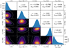 |
Fig. A.3 Same as Fig. 13 but only for clumps viewed from y direction. |
| In the text | |
|
Fig. A.4 As Fig. 13 but comparing default models at different distances. The background images and histograms plotted with black lines are for d = 152 pc. Data for distances d = 533 pc and d = 1232 pc are drawn with blue and red lines (and contours), respectively. The correlation coefficients in the frames above the diagonal arewritten in the corresponding colours. |
| In the text | |
|
Fig. B.1 Polarisation fraction associated to selected PGCC clumps. The first frame shows the relation p vs. intensity when both are measured at the clump centres. The second frame shows p as a functionof the estimated γ angle. The last frame shows the same for the p contrast (p at the clumpcentre divided by the average over radial distances 16–20′). The blue and red colours correspond to two clump samples (see text). The cyan and magenta lines show the corresponding median values calculated with a moving window with the width one tenth of the data range. |
| In the text | |
Current usage metrics show cumulative count of Article Views (full-text article views including HTML views, PDF and ePub downloads, according to the available data) and Abstracts Views on Vision4Press platform.
Data correspond to usage on the plateform after 2015. The current usage metrics is available 48-96 hours after online publication and is updated daily on week days.
Initial download of the metrics may take a while.