| Issue |
A&A
Volume 586, February 2016
|
|
|---|---|---|
| Article Number | A103 | |
| Number of page(s) | 35 | |
| Section | Interstellar and circumstellar matter | |
| DOI | https://doi.org/10.1051/0004-6361/201526538 | |
| Published online | 02 February 2016 | |
Consistent dust and gas models for protoplanetary disks
I. Disk shape, dust settling, opacities, and PAHs
1 SUPA, School of Physics & Astronomy, University of St. Andrews, North Haugh, St. Andrews KY16 9SS, UK
e-mail: pw31@st-andrews.ac.uk
2 UJF-Grenoble 1/CNRS-INSU, Institut de Planétologie et d’Astrophysique (IPAG) UMR 5274, 38041 Grenoble, France
3 Kapteyn Astronomical Institute, Postbus 800, 9700 AV Groningen, The Netherlands
4 Astronomical Institute “Anton Pannekoek”, University of Amsterdam, PO Box 94249, 1090 GE Amsterdam, The Netherlands
5 University of Vienna, Department of Astrophysics, Türkenschanzstrasse 17, 1180 Vienna, Austria
6 UMI-FCA, CNRS/INSU France (UMI 3386), and Departamento de Astronomíca, Universidad de Chile, 1058 Santiago, Chile
7 Departamento de Física Teórica, Universidad Autonoma de Madrid, Campus Cantoblanco, 28049 Madrid, Spain
8 Max Planck Institute for Extraterrestrial Physics, Giessenbachstrasse, 85741 Garching, Germany
9 Leiden Observatory, Leiden University, PO Box 9513, 2300 RA Leiden, The Netherlands
10 INAF, Osservatorio Astronomico di Cagliari, via della Scienza 5, 09047 Selargius (CA), Italy
11 Konkoly Observatory, Hungarian Academy of Sciences, 1121 Budapest, Konkoly Thege Miklós út 15−17, Hungary
12 Université de Toulouse, UPS-OMP, IRAP, 14 avenue É. Belin, 31400 Toulouse, France
13 Institute of Astronomy, University of Cambridge, Madingley Road, Cambridge CB3 0HA, UK
Received: 15 May 2015
Accepted: 4 November 2015
We propose a set of standard assumptions for the modelling of Class II and III protoplanetary disks, which includes detailed continuum radiative transfer, thermo-chemical modelling of gas and ice, and line radiative transfer from optical to cm wavelengths. The first paper of this series focuses on the assumptions about the shape of the disk, the dust opacities, dust settling, and polycyclic aromatic hydrocarbons (PAHs). In particular, we propose new standard dust opacities for disk models, we present a simplified treatment of PAHs in radiative equilibrium which is sufficient to reproduce the PAH emission features, and we suggest using a simple yet physically justified treatment of dust settling. We roughly adjust parameters to obtain a model that predicts continuum and line observations that resemble typical multi-wavelength continuum and line observations of Class II T Tauri stars. We systematically study the impact of each model parameter (disk mass, disk extension and shape, dust settling, dust size and opacity, gas/dust ratio, etc.) on all mainstream continuum and line observables, in particular on the SED, mm-slope, continuum visibilities, and emission lines including [OI] 63 μm, high-J CO lines, (sub-)mm CO isotopologue lines, and CO fundamental ro-vibrational lines. We find that evolved dust properties, i.e. large grains, often needed to fit the SED, have important consequences for disk chemistry and heating/cooling balance, leading to stronger near- to far-IR emission lines in general. Strong dust settling and missing disk flaring have similar effects on continuum observations, but opposite effects on far-IR gas emission lines. PAH molecules can efficiently shield the gas from stellar UV radiation because of their strong absorption and negligible scattering opacities in comparison to evolved dust. The observable millimetre-slope of the SED can become significantly more gentle in the case of cold disk midplanes, which we find regularly in our T Tauri models. We propose to use line observations of robust chemical tracers of the gas, such as O, CO, and H2, as additional constraints to determine a number of key properties of the disks, such as disk shape and mass, opacities, and the dust/gas ratio, by simultaneously fitting continuum and line observations.
Key words: stars: formation / circumstellar matter / radiative transfer / line: formation / astrochemistry / methods: numerical
© ESO, 2016
1. Introduction
Disk models are widely used by the community to analyse and interpret line and continuum observations from protoplanetary disks, such as photometric fluxes, low- and high-resolution spectroscopy, images and visibility data, from X-ray to centimetre wavelengths. Historically, disk models could be divided intocontinuum radiative transfer models, such as HOCHUNK3D (Whitney et al. 2003), MC3D (Wolf 2003), RADMC (Dullemond & Dominik 2004a), TORUS (Harries et al. 2004), MCFOST (Pinte et al. 2006) and MCMax (Min et al. 2009), to explore the disk shape, dust temperature and grain properties, and thermo-chemical models, see e.g. (Henning & Semenov 2013) for a review, and Table 1. The thermo-chemical models usually include chemistry and UV and X-ray physics to explore the temperature and chemical properties of the gas, with particular emphasis on the outer disk as traced by (sub-)mm line observations.
However, this distinction is becoming more and more obsolete, because new disk models try to combine all modelling components and techniques, either by developing single, stand-alone modelling tools likeProDiMo (Woitke et al. 2009) and DALI (Bruderer et al. 2014), or by coupling separate continuum and gas codes to achieve a similar level of consistency.
Assumptions about disk shape, grain size, opacities, dust settling and PAHs in different thermo-chemical disk models.
Observational data from protoplanetary disks obtained with a single observational technique in a limited wavelength interval can only reveal certain information about the physical properties at particular radii and at particular vertical depths in the disk. Therefore, in order to derive an overall picture of protoplanetary disks, it is essential to combine all observational data, and to make consistent predictions for all continuum and line observables in a large range of wavelengths on the basis of a single disk model.
However, this holistic modelling approach does not come without a price. The number of free parameters in such models is large (around 20), and the computational time required to run one model can exceed days, weeks or even months (e.g. Semenov et al. 2006). These limitations have resulted in quite limited parameter space being explored in such models.
Therefore, previous chemical models have not fully explored the role of disk shape and dust opacities. In Table 1, we list assumptions made in differnt thermo-chemical disk models about the shape of the disk, the dust size distribution, opacities, dust settling, and polycyclic aromatic hydrocarbons (PAHs). The selection of models is not exhaustive in Table 1, for a more comprehensive overview of modelling techniques and assumptions see Table 3 in (Henning & Semenov 2013). Table 1 shows the diversity of modelling assumptions currently used by different disk modelling groups. These models often focus on the outer disk, consider small dust particles, and use different approaches for dust settling and PAHs.
All these assumptions have crucial impacts on the modelling results, not only with regard to the predicted continuum observations, as known from SED fitting, but also on chemical composition and line predictions. Therefore, to compare modelling results from a large number of protoplanetary disks, a set of consistent standard modelling assumptions is required.
In this paper, we explore what could be a minimum set of physical assumptions about the star, the disk geometry, the dust and PAH opacities, dust settling, gas and ice chemistry, gas heating and cooling, and line transfer, needed to capture the most commonly observed multi-wavelength properties of Class II and III protoplanetary disks. We aim at a consistent, coupled modelling of dust and gas, and we want to predict the full suite of observations simultaneously and consistently from one model.
In Sect.2 we introduce our aims and basic approach, in Sect. 3 we describe the details of our model, and in Sect. 4 we cross-check and verify the implementation of our assumptions into our three main modelling tools ProDiMo, MCFOST, and MCMax. In Sect. 5, we show first results for a simple model of a Class II T Tauri star, and systematically study the impact of all modelling parameters on the various predicted observables. We summarise these results and conclude in Sect. 6.
In the Appendices, we collate a number of auxiliary information. We explain our fitting routine of stellar parameters including UV and X-ray properties (Appendix A), and describe our assumptions concerning interstellar UV and IR background radiation fields. We compare some results obtained with the simplified treatment of PAHs (see Sect. 3.8) against models using the full stochastic quantum heating method in Appendix B. Appendix C compares the results obtained with time-dependent chemistry against those obtained in kinetic chemical equilibrium. We detail how certain observable key properties are computed from the models in Appendix D. Appendix E discusses the behaviour of optically thick emission lines. In Appendix F, we discuss the convergence of our results as function of the model’s spatial grid resolution.
Two forthcoming papers will continue this paper series, to study the impacts of chemical rate networks (Kamp et al., in prep., Paper II) and element abundances (Rab et al. 2015, Paper III) on the resulting chemical abundances and emission lines. Kamp et al. introduce a simplified, small chemical rate network and a more exhaustive, large chemical network, henceforth called the small DIANA chemical standard and the large DIANA chemical standard, respectively.
2. The DIANA project
The European FP7 project DiscAnalysis (or DIANA) was initiated to bring together different aspects of dust and gas modelling in disks, alongside multiwavelength datasets, in order to arrive at a common set of agreed physical assumptions that can be implemented in all modelling software, which is a precondition to cross-correlate modelling results for different objects.
The DIANA goal is to combine dust continuum and gas emission line diagnostics to infer the physical and chemical structure of Class II and III protoplanetary disks around M-type to A-type stars from observations, including dust, gas and ice properties. The project aims at a uniform modelling of a statistically relevant sample of individual disks with coherent observational data sets, from X-rays to centimetre wavelengths.
In protoplanetary disks, various physical and chemical mechanisms are coupled with each other in complicated, at least two-dimensional ways. Turbulence, disk flaring, dust settling, the shape of the inner rim, UV and X-ray irradiation, etc., lead to an intricate interplay between gas and dust physics. Therefore, consistent gas and dust models are required. Each of the processes listed above can be expected to leave specific fingerprints in form of observable continuum and line emissions that can possibly be used for their identification and diagnostics.
However, to include all relevant physical and chemical effects in a single disk model is a challenging task, and we have decided to include only processes which we think are the most important ones, clearly with some limitations. We also want to avoid approaches that are too complicated and pure theoretical concepts that are not yet verified by observations. The level of complexity in the models should be limited by the amount and quality of observational data we have to check the results. The result of these efforts are our disk modelling standards that we are proposing to the community in this paper series.
New challenges for disk modelling have emerged with the advances in high-resolution imaging (e.g. ALMA, NACO, SPHERE and GPI). These observations show evidence for non-axisymmetric structures such as spiral waves, warps, non-aligned inner and outer disks, and horseshoe-like shapes in the sub-mm. In the future, 3D models are clearly required to model such structures, but these challenges go beyond the scope of this paper. This paper aims at setting new 2D disk modelling standards as foundation for the DIANA project, sufficient to reproduce the majority of the observations, simple to implement, yet physically established, and sufficiently motivated by observations. We will offer our modelling tools and collected data sets to the community1.
 |
Fig. 1 Three figures visualising our disk modelling approach concerning disk shape and dust settling. This particular model has two radial zones, with a (dust and gas-free) gap between r = 1 AU to r = 5 AU. The outer zone is featured by a tapered outer edge. The left plot shows the hydrogen nuclei particle density n⟨ H ⟩(r,z). The middle and right plots show the local gas/dust ratio, and the mean dust particle size, respectively. These two properties are not constant throughout the disk, but depend on r and z through dust settling, see Sect. 3.5. From top to bottom, the two red dashed contour lines show the radial optical depth, in terms of the visual extinction, AV,rad = 0.01 and AV,rad = 1, and the two dashed black contours show the vertical optical depths AV = 1 and AV = 10. In the middle and r.h.s. plots, the vertical AV = 10 contour line has been omitted. |
3. Standard disk modelling approach
3.1. Stellar parameters and irradiation
To model Class II protoplanetary disks, we need to specify the stellar and interstellar irradiation at all wavelengths. This requires determining the photospheric parameters of the central star, i.e. the stellar luminosity L⋆, the effective stellar temperature T⋆ and the stellar mass M⋆. From these properties, the stellar radius R⋆ and the stellar surface gravity log (g) can be derived. Fitting these stellar properties to photometric observations is essential for modelling individual disks, which requires knowing the distance d and determining the interstellar extinction AV. More details about our procedure for fitting the photospheric stellar properties are explained in Appendix A.
Young stars are known to be strong UV and X-ray emitters. This additional, non-photospheric, high-energy disk irradiation can be neglected for pure dust continuum models, but is essential for the modelling of the chemistry and energy balance of the gas in protoplanetary disks. In Appendices A.2 and A.3, we explain how observed UV spectra and measured X-ray data can be used to prescribe this additional high-energy irradiation in detail. If such detailed data is not available, we propose a 4-parameter prescription, the relative UV luminosity fUV = LUV/L⋆, a UV powerlaw index pUV, the X-ray luminosity LX and the X-ray emission temperature TX, see Appendices A.2 and A.3 for details. All stellar irradiation components (photosphere, UV, X-rays) are treated by one point source in the centre of the disk.
In addition to the stellar irradiation, the disk is also exposed to interstellar irradiation: the interstellar UV field, infrared background radiation, and the 2.7 K cosmic background. All these types of irradiation are treated by an additional isotropic irradiation, approaching the disk from all sides (see Appendix A.4).
3.2. Disk mass and column density structure
The gas column density structure Σ(r) [g/cm2] is assumed to be given by a radial powerlaw with index ϵ, modified by an exponential tapering off factor 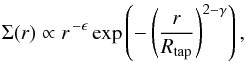 (1)where r is the radius and Rtap the tapering-off radius. This approach can naturally explain the often somewhat larger spectral appearance of protoplanetary disks in (sub-)mm molecular lines as compared to millimetre continuum images. If the disk has a tenous continuation, the lines remain optically thick to quite large radii, where the optically thin continuum signal already vanishes in the background noise. For example, the CO J = 2 → 1 line at 1.3 mm only requires a hydrogen nuclei column density of about NH = Σ/(1.4 amu) ≈ 10 21 cm-2 in our models to become optically thick, whereas the 1.3 mm continuum requires NH ≈ 2 × 10 24 cm-2. In our reference model (see Sect. 5.1), these column densities correspond to radii of about 450 AU and 20 AU, respectively.
While a tapering-off column density structure according to Eq. (1), with constant dust/gas ratio, seems sufficient to explain the different apparent sizes of gas and dust in many cases, for example (Isella et al. 2007; Tilling et al. 2012) for HD 163296 and (Panić et al. 2009) for IM Lupi, recent high S/N ALMA observations of TW Hya (Andrews et al. 2012) and HD 163296 (de Gregorio-Monsalvo et al. 2013) suggest that the radial extension of millimeter-sized grains can be significantly smaller, with a sharp outer edge, i.e. a varying dust/gas ratio. However, since the predicted timescales for radial migration are in conflict with current observations (e.g. Birnstiel & Andrews 2014), and not much is known quantitatively about migration yet, we assume a constant dust/gas ratio in this paper, to avoid the introduction of additional free parameters.
The default choice for the tapering-off exponent is γ = ϵ (self-similar solution, Hartmann et al. 1998). However, here the two exponents are kept independent, in order to avoid ϵ to be determined by γ in cases where high-quality sub-mm image data allow for a precise determination of γ. We think that the inner disk structure should rather be constrained by observations originating from the inner regions, for example near-IR excess, IR interferometry, ro-vibrational CO lines, etc.. Radial integration of Eq. (1), from Rin to Rout, results in the total disk mass Mdisk, which is used to fix the proportionality constant in Eq. (1). The inner rim is assumed to be sharp and positioned at Rin. The outer radius Rout ≫ Rtap is chosen large enough to ensure that Σ(Rout) is small enough to be neglected, e.g. NH(Rout) ≈ 1020 cm-2.
3.3. Vertical gas stratification
We assume a Gaussian vertical gas distribution with parametric gas scale height Hg as function of r as 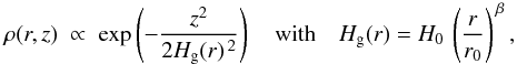 (2)where ρ(r,z) is the gas mass density in cylindrical coordinates, H0 is the reference gas scale height at radius r0, and β is the flaring exponent. Vertical integration of the gas density ρ(r,z) results in Σ(r) which is used to fix the proportionality constant in Eq. (2). We have chosen this simple approach to be most flexible with our fits of near-IR excess, far-IR excess, visibilities and gas lines. An alternative approach would be to assume vertical hydrostatic equilibrium, either using the calculated dust or gas temperature as input, but these models have some issues reproducing T Tauri disk observations, see Sect. 5.2.2. Also, such models take about 5× to 100× more computational time to complete, because an iteration between radiative transfer, gas physics, and vertical structure is required. This approach is not appropriate when considering the calculation of a large number of models, as is required when fitting observations.
3.4. Dust size distribution
We assume a powerlaw dust size distribution f0(a)[cm-4] as function of particle radius a [cm] as ![\begin{equation} f_0(a)\;\propto\;a^{-\apow} \quad\mbox{with}\quad a\in[\amin,\amax] . \label{eq:dustsize} \end{equation}](/articles/aa/full_html/2016/02/aa26538-15/aa26538-15-eq83.png) (3)Equation (3) prescribes the dust size distribution function in the disk “before settling”. Dust settling concentrates the larger grains toward the midplane, and therefore, the local dust size distribution f(a,r,z)[cm-4] will, in general, deviate from f0(a). Since dust settling only re-distributes the dust particles vertically in a given column, vertical integration over that column must again result in f0(a) = ∫f(a,r,z) dz/∫dz. The local dust mass density [g/cm3], before settling, is given by
(3)Equation (3) prescribes the dust size distribution function in the disk “before settling”. Dust settling concentrates the larger grains toward the midplane, and therefore, the local dust size distribution f(a,r,z)[cm-4] will, in general, deviate from f0(a). Since dust settling only re-distributes the dust particles vertically in a given column, vertical integration over that column must again result in f0(a) = ∫f(a,r,z) dz/∫dz. The local dust mass density [g/cm3], before settling, is given by  , where ρd is the dust material density, ρ the gas density and δ the assumed unsettled dust/gas mass ratio. This condition is used to fix the proportionality constant in Eq. (3).
The minimum and maximum dust size, amin and amax, are set by the following simple considerations: sub-micron sized particles are directly seen in scattered light images, high above the midplane. They are abundant in the interstellar medium (larger grains up to a few μm seem to already exist in dense cores, see Lefèvre et al. 2014), and disks are primordially made of such dust. Millimetre sized grains do also exist in protoplanetary disks, as indicated by the observed SED slope at mm-wavelengths. Therefore, a powerlaw covering the entire size range seems to be the most simple, straightforward option. We will explore the effects of amin, amax and apow on the various continuum and line observations in Sect. 5.2.1.
3.5. Dust settling
Dust settling is included according to Dubrulle et al. (1995), assuming an equilibrium between upward turbulent mixing and downward gravitational settling. The result is a size and density-dependent reduction of the dust scale heights Hd(r,a) with respect to the gas scale height Hg(r), ![\begin{eqnarray} && \left(\frac{H_{\rm d}(r,a)}{H_{\rm g}(r)}\right)^{2} = \frac{(1+\gamma_0)^{-1/2}\,\alpha_{\rm settle}} {\tau_{f}(r,a)\;\Omega(r)} \label{eq:settle}\\[3mm] &&\tau_{f}(r,a) = \frac{\rho_{\rm d}\;a}{\rho_{\rm mid}(r)\;c_T(r)}, \label{eq:tauf} \end{eqnarray}](/articles/aa/full_html/2016/02/aa26538-15/aa26538-15-eq95.png) where Ω(r) is the Keplerian orbital frequency, γ0 ≈ 2 for compressible turbulence, and τf(r,a) is the frictional timescale in the Stokes regime. ρmid(r) is the midplane gas density, and cT the midplane sound speed. To avoid iterations involving the midplane temperature as computed by dust radiative transfer, we use cT(r) = Hg(r) Ω(r) here, where Hg(r) is the gas scale height from Eq. (2). αsettle is the dimensionless viscosity parameter describing the strength of the turbulent mixing. The l.h.s. of Eq. (4) is smoothly limited to a maximum value of one by y2 → y2/ (1 + y2) with y = Hd(r,a) /Hg(r). Technically, in every disk column, Eq. (4) is computed for a number of (about 100) dust size bins. Starting from the unsettled dust size distribution, the dust particles in each size bin are re-distributed in z-direction according to f(a,r,z) ∝ exp(−z2/ [2Hd(r,a) 2]), building up a numerical representation of the local dust size distribution function at every point in the disk f(a,r,z).
where Ω(r) is the Keplerian orbital frequency, γ0 ≈ 2 for compressible turbulence, and τf(r,a) is the frictional timescale in the Stokes regime. ρmid(r) is the midplane gas density, and cT the midplane sound speed. To avoid iterations involving the midplane temperature as computed by dust radiative transfer, we use cT(r) = Hg(r) Ω(r) here, where Hg(r) is the gas scale height from Eq. (2). αsettle is the dimensionless viscosity parameter describing the strength of the turbulent mixing. The l.h.s. of Eq. (4) is smoothly limited to a maximum value of one by y2 → y2/ (1 + y2) with y = Hd(r,a) /Hg(r). Technically, in every disk column, Eq. (4) is computed for a number of (about 100) dust size bins. Starting from the unsettled dust size distribution, the dust particles in each size bin are re-distributed in z-direction according to f(a,r,z) ∝ exp(−z2/ [2Hd(r,a) 2]), building up a numerical representation of the local dust size distribution function at every point in the disk f(a,r,z).
We consider dust settling as a robust physical effect that should occur rapidly in any disk (Dullemond & Dominik 2004b), with the dust grains relaxing quickly toward a vertical equilibrium distribution as described by Eq. (4). Therefore, we think this important effect should be included in radiative transfer as well as in thermo-chemical disk models. Equations (4) and (5) offer an easy-to-implement, yet physically well-justified method to do so, with just a single parameter αsettle.
3.6. Radial zones, holes, and gaps
There is increasing evidence that protoplanetary disks are frequently sculptured by the planets forming in them, which results in the formation of various shape defects, in particular disk gaps (e.g. Forrest et al. 2004; Andrews et al. 2011; Kraus et al. 2013). The gaps are apparently mostly devoid of dust, but may still contain gas as traced by CO rotational and ro-vibrational emission lines (e.g. Bruderer 2013; Carmona et al. 2014). Such objects are classified as transitional disks, with a strong deficiency of near-IR to mid-IR flux. Understanding the SEDs of transitional disks requires to position the inner wall of the (outer) disk at much larger radii than expected from the dust sublimation temperature or the co-rotation radius (e.g. Espaillat et al. 2014). The physical mechanisms responsible for gap formation and disk truncation are still debated, for example planet formation and migration (Lin & Papaloizou 1986; Trilling et al. 1998; Nelson et al. 2000; Zhang et al. 2014), and/or photo-evaporation winds (Font et al. 2004; Alexander et al. 2006; Gorti & Hollenbach 2009), but one observational fact seems to have emerged: disk shape defects are common. In fact, single-zone, continuous protoplanetary disks (e.g. FT Tau, see Garufi et al. 2014) could be a rather rare class (e.g. Maaskant et al. 2014), and for the modelling of individual protoplanetary disks we need an additional option. For an archetypal shape defect, we consider two distinct radial disk zones, with a gap in-between. In such a case, all disk shape, dust and settling parameters come in two sets, one for the inner zone, and one for the outer zone.
3.7. Standard dust opacities
As we will show in this paper, the assumptions about the dust opacities have a crucial impact not only on the predicted continuum observations, but also for chemistry and emission lines. Therefore, the authors of this paper have agreed on a new common approach, which includes a number of robust facts and requirements that are essential to model disks. We will explain these new standard dust opacities carefully in the following, because we think that the dust in disks is different from the dust in the interstellar medium and standard dust opacities so far only exist for the interstellar medium (e.g. Draine & Lee 1984; Laor & Draine 1993).
Our assumptions for the dust opacity treatment are guided by a study of multi-wavelength optical properties of dust aggregates (Min et al. 2016) where the Discrete Dipole Approximation (DDA) is used to compute the interaction of light with complexly shaped, inhomogeneous aggregate particles. These opacity calculations are computationally too expensive to be applied in complex disk models, but Minet al. have developed a simplified, fast numerical treatment that allows us to reproduce these opacities reasonably well.
We consider a mixture of amorphous laboratory silicates (Dorschner et al. 1995, Mg0.7Fe0.3SiO3) with amorphous carbon (Zubko et al. 1996, BE-sample). Pure laboratory silicates are “glassy” particles with almost negligible absorption cross sections in the near-IR, just where T Tauri stars are most luminous. Such particles would rather scatter the incident light away from the disk, which would lead to substantial problems in explaining the near-IR excess of T Tauri stars. Therefore, the inclusion of a conductive, hence highly opaque, albeit featureless material in the near-IR is necessary. However, it is unclear whether amorphous carbon, metallic iron, or e.g. troilite (FeS) should be used. Our simplified material composition is inspired by the past disk modelling expertise of the team, and by the solar system composition proposed by Min et al. (2011).
The dust grains are assumed to be composed of 60% silicate, 15% amorphous carbon, and 25% porosity, by volume, well-mixed on small scales. The effective refractory index of this porous material is calculated by applying the Bruggeman (1935) mixing rule. In contrast, just adding opacities (assuming separate grains of pure materials with the same size distribution and equal temperatures) does not seem physically justified at all, and does not reproduce the optical properties of aggregate particles equally well (Min et al. 2016).
We use a distribution of hollow spheres (DHS) with a maximum hollow volume ratio  . This approach avoids several artefacts of Mie theory (spherical resonances) and can account for the most important shape effects, see details in (Min et al. 2016). In combination with our choice of the amorphous carbon optical constants from Zubko et al. (1996, BE-sample), this approach captures the “antenna-effect” observed from the aggregate particles, where irregularly shaped inclusions of conducting materials result in a considerable increase of mm-cm absorption opacities.
Table 3 summarises our standard choices of dust parameter values, and Fig. 2 shows the resulting opacities including scattering and extinction. Figure 3 shows the dependencies of the dust absorption opacities on the remaining free dust size and material parameters. We will continue to discuss these results and their impact on predicted continuum and line observations in Sect. 5.2.1. Our standard dust opacities feature
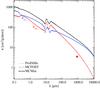 |
Fig. 2 Dust opacities used for the standard disk radiative transfer modelling, with parameters amin = 0.05 μm, amax = 3 mm, apow = 3.5, and 15% amorphous carbon by volume. The extinction per dust mass is shown in black, absorption in red, and scattering in blue. Results shown with lines for ProDiMo, open symbols for MCMax, and full symbols for MCFOST – all of which agree. The red star represents the value of 3.5 cm2/ g(dust) at 850 μm used by Andrews & Williams (2005) to determine disk masses from sub-mm fluxes. |
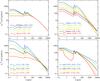 |
Fig. 3 Dust absorption coefficient per dust mass as function of dust size and material parameters. The black line is identical in every part plot, with parameter values as used in the reference model, our dust standard opacities, see Table 3. The upper two figures show the dependencies on minimum and maximum particle size, amin and amax. The lower two plots show the dependencies on dust size powerlaw index apow and on the volume fraction of amorphous carbon. 25% porosity and maximum hollow volume ratio |
-
a FUV-dust extinction opacity of about 1000 cm2/g(dust), which is about 100 times less than in standard ISM models with MRN size distribution (Mathis et al. 1977);
-
a dust albedo of 64% at FUV wavelengths, and 58% at 1 μm;
-
a dust absorption cross section of about 5.8 cm2/g(dust) at 850 μm, which is about a factor of 1.6 larger than the value of 3.5 cm2/g(dust) used by Andrews & Williams (2005) to determine disk masses from sub-mm fluxes2;
-
a millimetre dust absorption slope of about 1; and
-
a centimetre dust absorption slope of about 1.5.
The dust opacities described above have been determined from the well-mixed dust size distribution function f0(a), see Sect. 3.4. Since we have dust settling in the disk, the dust opacities need to be computed from the local settled dust size distribution function f(a,r,z), and will hence not only depend on λ, but also on the location in the disk (r,z). Simply put, dust settling leads to a strong concentration of the (sub-)mm opacity in the midplane, in particular in the outer disk regions, but only to a mild reduction of the UV opacities in the upper and inner layers. According to Fig. 3, the main effects are:
-
1)
Large amin values reduce the optical and UV opacities, and destroy the 10 μm/20 μm silicate emission features.
-
2)
Large amax values reduce the UV, optical, near-IR and far-IR opacities considerably, because the available dust mass is spread over a larger size range, and the big particles do not contribute much to the dust opacities at those wavelengths. Here, increasing amax has similar consequences as lowering the dust/gas mass ratio. At longer wavelengths, amax determines where the final transition to the Rayleigh-limit takes place (λtrans ≈ 2πamax), beyond which (λ>λtrans) the opacity changes to a steeper slope. For larger amax, this transition occurs at longer wavelengths. The choice of our reference value of amax = 3 mm is motivated by cm-observations which usually do not show such breaks. However, Greaveset al. (in prep.) report on first evidence of such a steepening toward cm wavelengths after removal of the free-free emission component, based on new Green Bank Telescope data up to 8.6 mm.
-
3)
The powerlaw size index apow determines the mixing ratio of small and large grains. Since the smaller particles are responsible for the short wavelength opacities, and the large grains for the long wavelength opacities, apow determines the general opacity slope, and the mm and cm-slopes in particular.
-
4)
A large volume fraction of amorphous carbon reduces the 10 μm, 20 μm silicate emission features, fills in the opacity deficits of the major solid-state silicate resonances (up to about 8 μm), and flattens the absorption opacities at millimetre and centimetre wavelengths.
In order to facilitate the adoption of these opacities in other work, a Fortran-90 package to compute the DIANA standard dust opacities3.
3.8. PAHs
Polycyclic aromatic hydrocarbon molecules (PAHs) play an important role in our disk models via (i) continuum radiative transfer effects; (ii) photoelectric heating of the gas; and (iii) chemical effects. The chemical effects include the charging of the PAHs, the release and consumption of free electrons via photo-ionisation and recombination, and further effects due to charge exchange reactions. We study (i) and (ii) for neutral PAHs in this paper, but do not include the chemical effects as we are using here the small DIANA chemical standard. In contrast, the large DIANA chemical standard (Paper II) has the PAHs included in the selection of chemical specimen, and therefore accounts for (iii) as well.
PAHs are observed via their strong mid-IR emission bands in many Herbig Ae/Be stars (e.g. Maaskant et al. 2014), whereas detection rates in T Tauri stars are much lower (Geers et al. 2006), possibly because T Tauri stars generate much less blue and soft UV stellar radiation to heat the PAHs. PAHs in Herbig Ae/Be disks seem to have sizes of at least 100 carbon atoms (Visser et al. 2007). The PAH abundance in the disk is assumed to be given by the standard abundance in the interstellar medium (Tielens 2008), modified by factor fPAH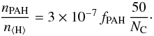 (6)fPAH = 1 corresponds to the interstellar medium (ISM) standard4. Here, nPAH [cm-3] is the PAH particle density, n⟨ H ⟩ [cm-3] is the hydrogen nuclei density and NC is the number of carbon atoms in the PAH. The actual PAH abundance in disks is disputed (e.g. Geers et al. 2006; Visser et al. 2007). Values fPAH ≈ 0.1 or lower seem typical in Herbig Ae disks (Geers et al. 2006).
We assume NC = 54 carbon atoms and NH = 18 hydrogen atoms (“circumcoronene”) in the reference model, resulting in a PAH mass of 667 amu and a PAH radius of 4.87 Å (Weingartner & Draine 2001). NC and fPAH are free model parameters, as well as a decision whether to select the neutral or charged PAH opacities. Circumcoronene IR and UV spectra have been directly measured by Bauschlicher Jr. & Bakes (2000). However, in the DIANA framework, we use “synthetic” PAH opacities of neutral and charged PAHs are calculated according to Li & Draine (2001) with updates from Draine & Li (2007), including the “graphitic” contribution in the near-IR and the additional “continuum” opacities of charged PAHs.
In comparison to the low UV opacities of evolved dust in disks (Sect. 3.7), PAHs can easily dominate the blue and UV opacities, see Fig. A.2. This happens in the well-mixed case for fPAH ≳ 0.1 in our disk models. The dominance of the PAH opacities in the UV is even stronger in the upper disk regions because of dust settling (we assume that PAH molecules do not settle). For Herbig Ae disks, where the maximum of the stellar radiation is released around 400 nm, fPAH ≳ 1 would imply that the stellar photons are predominantly absorbed by the PAHs rather than by the dust. The absorbed energy would then be re-emitted via the strong PAH mid-IR resonances, and it is this mid-IR PAH emission that would predominantly heat the disk. Furthermore, the stellar UV usually reaches the line forming regions in a disk indirectly, via scattering on dust particles from above. For fPAH ≳ 0.1, the PAHs would effectively shield the disk from UV radiation, because UV scattering by PAHs is extremely inefficient. These two effects have large implications on our models for both the internal dust and gas temperature structure in a disk.
The treatment of PAHs in the Monte Carlo programs MCFOST and MCMax is standard, using a quantum heating formalism with stochastic PAH temperature distribution. This mechanism was first proposed for small grains by Desert et al. (1986) and later applied to PAHs in the interstellar medium by Manske & Henning (1998), Guhathakurta & Draine (1989), Siebenmorgen et al. (1992). The Monte Carlo programs offer additional options to take into account e.g. a PAH size distribution and an internal determination of the PAH charge, by balancing the basic photo-ionisation and recombination rates (Maaskant et al. 2014). However, these options involve some quite specific simplifications, for example no negative PAHs, no charge exchange reactions, and an assumed electron concentration, which we need to avoid for reasons of consistency for the DIANA modelling efforts.
While looking for a fast, simplified, and robust way to treat the most important effects of PAHs equally well in all our disk models, we discovered that a simplified treatment of the PAHs in radiative equilibrium, according to 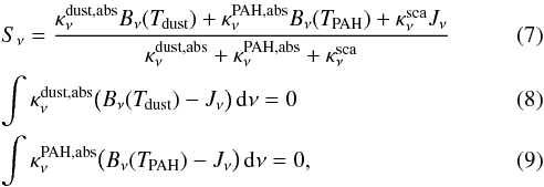 leads to quite accurate results in comparison to the stochastic PAH treatment, see Appendix B and Fig. A.3. Here, Sν is the source function,
  and
and  are the absorption and scattering opacities (of dust and PAHs as annotated), Bν(T) is the Planck function and Jν is the mean intensity. The scattering term
  is here simplifyingly written for isotropic scattering. Equations (8) and (9) express the conditions of radiative equilibrium with separate dust and PAH temperatures, Tdust and TPAH, respectively.
The quantum heating formalism is appropriate for ISM conditions, where PAHs are only sometimes heated by rare FUV photons. In contrast, we show in Appendix B that the PAHs in the inner regions of protoplanetary disks, which are responsible for the observable mid-IR PAH emission features, are situated in an intense optical and infrared radiation field created by the star and by the dust and the PAHs in the disk, which keeps the stochastic PAH temperature distribution high and quite narrow, i.e. close to the analytical treatment in radiative equilibrium. Li & Mann (2012) found similar results for nano grains acquiring an equilibrium temperature when exposed to intense starlight.
3.9. Chemistry and heating/cooling balance
Based on the results of the continuum radiative transfer as described in the previous sections, the gas phase and ice chemistry is calculated in kinetic chemical equilibrium, coupled to the gas heating/cooling balance. These parts of the model have been described elsewhere, see (Woitke et al. 2009) for the basic model, (Thi et al. 2011) for continuum radiative transfer, (Woitke et al. 2011) for updates concerning non-LTE treatment and heating and cooling, and (Aresu et al. 2011) for X-ray heating and chemistry, and are not discussed in this paper. In this paper we use the small chemical network, as proposed in Paper II. We carefully select 100 gas phase and ice species (see Paper II), and take into account altogether 1288 reactions. All 1065 gas phase and UV reactions among the selected species are taken into account from the UMIST 2012 database (McElroy et al. 2013), including the old collider reactions. We replace the treatment of photo-reactions by individual photo cross-sections from the Leiden Lamda database (Schöier et al. 2005) where possible, add 145 X-ray reactions (Aresu et al. 2011), 40 ice adsorption and thermal, UV photo and cosmic ray desorption reactions, and 38 auxiliary reactions including those of vibrationally excited molecular hydrogen H , see details in Paper II. We take the (gas + ice) element abundances from Table 2 in Paper III. Appendix C discusses the validity of our approach to use the time-independent solution of our chemical rate network to compute the chemical composition of the disk and the gas emission lines.
Unsettled dust properties in the reference model in comparison to a MRN size distribution and uniform a = 0.1 μm dust particles.
Model parameters, and values for the reference model.
3.10. Line radiative transfer
After the continuum radiative transfer, gas and dust temperature structure, chemistry and non-LTE level populations have been determined, a formal solution of line and continuum radiative transfer is carried out in 3D, using a bundle of 356 × 144 parallel rays towards the observer at distance d under inclination angle i, see (Woitke et al. 2011, Appendix A.7 therein) for details. These computations result in observable quantities like line fluxes, line velocity-profiles, molecular line maps and channel maps.
4. Model implementation and verification
The DIANA standard modelling assumptions summarised in Sect. 3 (stellar and interstellar irradiation, disk shape, dust opacities, dust settling, treatment of PAHs) have been implemented into MCFOST (Pinte et al. 2006, 2009) MCMax (Min et al. 2009) and ProDiMo (Woitke et al. 2009). The independent implementation of our modelling assumptions has allowed us to perform stringent checks on our computational methods and numerical results. Figure 2 shows a validation of our dust opacity implementation. Figure A.2 compares the assumed gas calculated settled dust densities, the resulting dust and PAH temperatures, as well as the SEDs. Apart from some minor temperature deviations in the optically thick midplane regions, which are irrelevant for the predicted observations, we achieve an excellent agreement concerning the physical state of the disk and all predicted observations. In particular, the upper right part of Fig. A.2 shows that we obtain very similar SED and spectral shape of the PAH features no matter whether we useProDiMo, MCFOST, or MCMax.
Further verification tests (not shown here) have been undertaken for disk models with gaps, where the numerical resolution of the inner wall of the outer disk is particularly important, and for MC → ProDiMo “chain models”. In these chain models, we use the Monte Carlo codes to compute the disk structure, the dust and PAH temperatures, and the internal radiation field Jν(r,z), and then pass these results on to ProDiMo to compute the gas temperature structure, the chemical composition of ice and gas, and the emission lines.
The advantages of using the MC → ProDiMo chain models are (i) the Monte-Carlo technique is computationally faster; (ii) the temperature iteration scheme is more robust, in particular at high optical depths; and (iii) the Monte-Carlo technique allows for a more detailed implementation of radiation physics, in particular anisotropic scattering, PAHs with stochastic quantum heating, and polarisation. For the effects of anisotropic scattering, see Fig. G.2 in Appendix G. These more sophisticated options are not used in this paper, in order to facilitate comparisons to the results obtained with pureProDiMo. The pre-existing interface between MCFOST andProDiMo (Woitke et al. 2010) has been generalised and implemented in MCMax, such that now all MCFOST and MCMax users are able to use ProDiMo to predict chemical and line results on top of their continuum models.
Appendix F discusses the numerical convergence of our models as function of numerical grid resolution, for both the pure ProDiMo and the MC → ProDiMo chain models. Our conclusion here is that we need about 100 × 100 grid points in both ProDiMo and MC models, to achieve an accuracy <10% for all continuum observables and line flux predictions.
5. Results
The results of our disk models are presented in the following way. We first introduce a simple single-zone reference model in Sect. 5.1 which roughly fits a number of typical continuum and line observations of Class II T Tauri stars. In the following two sub-sections, we then study the impact of our model parameters on the various continuum and line observables by looking at how our model predictions change with respect to the reference model. In Sect. 5.2, we study the impact of selected model parameters on all observables at a time, and in Sect. 5.3, we discuss particular observables separately.
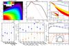 |
Fig. 4 Summary of results from the reference model. Top row: assumed gas density structure n⟨ H ⟩(r,z) with overplotted radial (red) and vertical (black) optical depths AV = 1 dashed contours, computed SED, and visibilities. In the visibility plot, the coloured areas show V2 for all baseline orientations at 3 different wavelengths, with a zoom-in on the first 30 m. Lower row: other resulting quantities. The left plot shows the mean dust and gas temperatures (in units of 10 K), the near-IR excess (in units of 0.05 L⊙) and the logarithmic SED slopes at mm and cm wavelengths. The centre plot shows calculated line fluxes and full widths at half maximum (FWHM). The right plot shows some results for the CO fundamental ro-vibrational line emissions, line fluxes as function of rotational quantum number J for the R-branch and the P-branch, as well as computed FWHM for those lines. The inserted figure shows the line profile averaged over all emission lines, scaled from 0 (continuum) to 1 (maximum). |
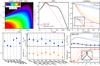 |
Fig. 5 Results from the T Tauri reference model, but assuming uniform 0.1 μm sized dust particles and astronomical silicate Mie opacities. Depicted quantities are shown with respect to the reference model, and explained in the caption of Fig. 4. |
5.1. The reference model
Table 3 summarises our model parameters, and lists the values used for the reference model. The resulting spectral energy distribution (SED), visibilities, line observations, and some integrated properties are shown in Fig. 4. Concerning the integrated properties, we calculate the mean gas temperature in the disk ⟨ Tgas ⟩, the mean dust temperature ⟨ Tdust ⟩, the near-IR excess, the 10 μm SED amplitude, the mm-slope and the cm-slope as explained in Appendix D, see Eqs. (D.1) to (D.8). The reference model is characterised by
-
a near-IR excess of about 0.12 L⊙;
clearly visible silicate dust emission features around 10 μm and 20 μm;
a descending SED-slope dlog (νFν)/dlog λ< 0 beyond 20 μm, as is typical for continuous (i.e. non-transitional) T Tauri disks;
a 1.3 mm continuum flux of 60 mJy with an apparent radius (semi-major axis) of about 100 AU (0.75″ at a distance of 140 pc) – typical observed values are about 20−200 mJy, and 0.25′′−1.4′′, see (Guilloteau et al. 2011);
a mm-slope of about 2.4 – typical observed values are about 1.9−2.7, see (Ricci et al. 2010, 2012);
a [OI] 63 μm line flux of 25 × 10-18 W/m2 – typical observed values for non-outflow sources are about (3−50) × 10-18 W/m2, see (Howard et al. 2013);
a 12CO J = 2 → 1 line flux of about 15 Jy km s-1, and a 12CO/13CO line ratio of about 5 – for typical values, see (Williams & Best 2014);
an apparent radius (semi-major axis) in the 12CO J = 2 → 1 line of about 450 AU (3.5″ at 140 pc), typical observed values are about 1″−5″, see (Williams & Best 2014);
weak CO ro-vibrational lines with a broad, box-shaped emission profile mostly emitted from the far side of the inner rim, which are not very typical with respect to observations. The “central nose” on top of the averaged line profile is a contribution from low-J lines which are also emitted from more distant disk regions, see Fig. 17. For typical CO ro-vibrational observations, see Sect. 5.3.7.
All other emission lines in the IR to far-IR spectral region are rather weak, which would likely result in non-detections with current instruments (for example o-H2O 63.3 μm, CO J = 18 → 17, o-H2 17.03 μm), maybe except for the optical [OI] 6300 Å line (model flux 7 × 10-18 W/m2). The CO fundamental ro-vibrational lines are also rather weak in the reference model (of order 2 × 10-18 W/m2 at FWHM = 130 km s-1), which is below the detection limit of e.g. the CRIRES spectrograph (about 10-18 W/m2 at FWHM = 20 km s-1).
5.2. Impact of selected model parameters
5.2.1. Dust size and opacity parameters
It is important to realise that dust grains in protoplanetary disks are likely to be very different from the tiny dust particles in the diffuse interstellar medium (ISM) for which the astronomical silicate opacities have been constructed by Draine & Lee (1984), only considering λ< 1 μm, and using MRN (Mathis et al. 1977) size parameters. In contrast, we expect the dust grains in disks to be much larger, up to mm-sizes, which reduces the UV dust opacities by a large factor (about 100) depending on parameters amin, amax and apow, see Table 2 and Fig. 3.
This simple and straightforward fact distinguishes our disk models from other chemical models (Table 1). In our models, the dust is much more transparent in the UV, allowing the UV to penetrate deeper into the disk, which increases the importance of molecular self-shielding, and reduces the importance of X-rays relative to the UV.
Table 2 shows that a disk-typical dust size distribution can be expected to have additional substantial impacts on disk chemistry, see also Vasyunin et al. (2011). The total grain surface area per H nucleus, important for surface chemistry, H2 formation and photoelectric heating, is reduced by a factor of about 250 with respect to the MNR dust model, and the dust particle concentration nd/n⟨ H ⟩ is only of order 10-14, where  is the (unsettled) total dust particle density. This implies, for example, that even if every dust grain was negatively charged once, there would be hardly any effect on the midplane electron concentration.
Figure 5 shows the results of the model when switching to uniform 0.1 μm sized dust particles and astronomical silicate opacities. The SED is now featured by stronger 10 μm/20 μm silicate emission features, higher far-IR continuum fluxes, and a quite sudden kink around 200 μm, followed by a steeper decline toward millimetre wavelengths. The apparent size of the disk is smaller at 1.6 μm, but larger at 10 μm and 1.3 mm. The disk is now warmer in dust, but cooler in gas, in fact mean dust and gas temperatures are more equal. Most emission lines in the model with uniform 0.1 μm dust particles show weaker fluxes, by up to a factor of ten. However, the CO J = 10 → 9 line doesn’t follow this general trend.
Understanding the impact of the dust size and material parameters on gas temperature and emission lines can be isolated to the effect of a single quantity, namely the dust optical depths at UV wavelengths τUV, see Sects. 5.3.4, 5.3.5 and 5.3.7. All dust parameter alterations that result in lower τUV will generally lead to a deeper penetration of UV into the disk, causing an increase of the thickness of the warm molecular gas layer, and this leads to stronger emission lines at optical to far-IR wavelengths. The impact is less pronounced on (sub-)mm lines, see Sect. 5.3.6, although secondary temperature and chemical effects are important to understand the (sub-)mm line ratios.
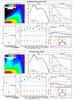 |
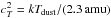
Fig. 6 Two variants of (1 + 1)D hydrostatic disk models. Depicted quantities are explained in Fig. 4, but shown here in comparison to the reference model. The upper half shows the results for the simplified hydrostatic model based on the dust temperature Tdust and a constant molecular weight, i.e. sound speed |

5.2.2. Hydrostatic disk models
Figure 6 summarises the results of two variants of (1+1)D hydrostatic models, where the vertical disk extension at any radius is computed from the condition of hydrostatic equilibrium, which requires an iterative approach of radiative transfer, chemistry and gas heating/cooling balance, see (Woitke et al. 2009) for details. The lower model is the proper hydrostatic solution, where the pressure p = ρkTgas/μ is calculated according to the local gas temperatures Tgas and mean molecular weight μ resulting from chemistry. The upper model is a simplified version thereof, where the dust temperature is used instead (Tgas ≈ Tdust), and the mean molecular weight is assumed to be constant (μ ≈ 2.3 amu). The observable properties of these hydrostatic models are as follows.
-
The SEDs of both types of hydrostatic models cannot explain the observed levels of near-IR excess for T Tauri stars, because the inner rim is quite low.
-
Between 20μm and 50μm, the SED displays an increasing slope, which is caused by the strong flaring of the outer disk (see also Fig. 2 in Meijerink et al. 2012).
-
The models are substantially warmer, both in gas and dust, as compared to the reference model, again because of the flaring of the outer disk.
-
The far-IR to mm emission lines are all stronger as compared to the reference model. The [OI] 63.2 μm flux is (7−10) × 10-17 W/m2, which is out 4 times stronger as in the reference model, and quite high with respect to observations. The 12CO/13CO line ratio is as large as 8.
-
The ro-vibrational CO ro-vibrational lines are weaker, because of the low inner rim, and have complicated multi-component line profiles.
The two variants of hydrostatic models have quite similar observable properties, including the spectral lines, although the disk gas density structure is remarkably different. The proper hydrostatic model displays larger amounts of extended hot gas high above the disk in the inner regions. However, this highly extended hot gas is purely atomic, hence it does not emit in molecular lines, one has to use atomic tracers to detect it, such as [OI] 6300 Å or maybe [NeII] 12.82 μm. In summary, hydrostatic passive disk models have some issues explaining the observed SED and line properties of T Tauri stars.
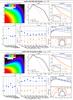 |
Fig. 7 Effects of disk flaring and dust settling on all observables, with respect to the reference model. The upper set of figures shows a model with less flaring as compared to the reference model β = 1.05, and the lower half shows a model with stronger dust settling αsettle = 10-4. See Fig. 6 for further explanations. |
5.2.3. Disk flaring and/or dust settling?
Little disk flaring and strong dust settling have similar effects on the SED, see Fig. 7. The β = 1.05 and αsettle = 10-4 models have practically indistinguishable SEDs beyond 20 μm, with a more steeply decreasing slope as compared to the reference model around ~ 50 μm. The reason for that steeper slope is that a more self-shadowed dust configuration leads to less interception of star light per disk radius interval, hence to a steeper decline of the dust temperatures as function of radius (e.g. Beckwith et al. 1990; Chiang & Goldreich 1997). We can see from Fig. 7 that indeed the mass averaged dust temperature ⟨ Tdust ⟩, which is dominated by the outer disk regions, has fallen from about 19 K in the reference model to about 13 K in both cases. Lacking disk flaring and strong dust settling both cause very low dust temperatures in the midplane, of order 4 K already at r = 150 AU in the αsettle = 10-4 model, only limited by CMB and other background radiation. These very cold disk models have particular mm and cm-properties, because the cold dust is not entirely emitting in the Rayleigh-Jeans limit even at millimetre wavelengths, see Sect. 5.3.3.
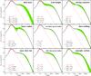 |
Fig. 8 Effect of dust and disk parameters on model SED at distance 140 pc and inclination 45°. The thick full black line is the reference model (identical in every part figure), whereas the green shaded area indicates the effect of a single parameter on the SED, where the dashed and dotted lines correspond to the changed parameter values as annotated. Top row: dust mass Mdust, scale height H0, and flaring exponent β. Second row: inner radius Rin, column density powerlaw index ϵ, and dust settling parameter αsettle. Third row: maximum grain size amax, dust size powerlaw index apow, and volume ratio of amorphous carbon. The dependencies of the SED on the tapering-off radius Rtap (not shown), on the outer radius Rout (not shown), and on the minimum dust particle size amin (not shown) are less than the one shown for ϵ. |
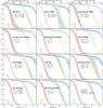 |
Fig. 9 Effects of selected dust and disk shape parameters on continuum visibilities at 1.6 μm (blue), 10 μm (green) and 1.3 mm (red). Distance is 140 pc. The squared visibility V2 (fraction of correlated flux) is shown as function of baseline [cm] /1000 /λ [cm] for baseline orientation along the major axis of the disk on the sky. The abscissa on top is the corresponding maximum observable spatial scale [cm] = 0.6·d [cm] /baseline [kλ] /1000. The full lines show the reference model, identical in every part figure. The dashed and dotted lines correspond to the changed parameter values as annotated. Non-depicted parameters have less influence on the visibilities, for example amax. See Table 3 for explanations of parameter symbols. |
Since the scale height is anchored at r = 100 AU in the model, little flaring (the β = 1.05 model) implies a tall inner disk which causes a strong near-IR excess. Assuming strong dust settling instead avoids these artefacts, because the impact of dust settling is strongest where the gas densities are lowest, i.e. in the outer regions, whereas the inner regions are only affected a little.
When looking at the impact on gas temperature and emission lines, however, the two models show just opposite effects. Lacking disk flaring moves the gas into the disk shadow, causing lower gas temperatures and weaker emission lines. Dust settling, in contrast, leaves the gas bare and exposed to the stellar UV radiation, leading to higher gas temperatures and stronger gas emission lines in general.
Therefore, in order to diagnose lacking disk flaring and/or strong dust settling, the far-IR SED slope around 50 μm is crucial, but to distinguish between disk flaring and dust settling, the simultaneous observation of far-IR gas lines is the key.
5.3. Parameter impact on selected observables
5.3.1. SED
Figure 8 shows the impact of our model parameters on the calculated spectral energy distribution (SED). Some parameter dependencies have already been discussed and explained in Sects. 5.2.1 and 5.2.3, but we repeat the essence here to give a comprehensive overview of all important effects.
The dust mass Mdust shifts the SED up and down at long wavelength, where the disk is predominantly optically thin. Its influence diminishes at λ ≲ 100 μm, but even at 20 μm, where the disk is massively optically thick, a change of Mdust still produces noticeable changes. This is because more mass increases the height at which the disk becomes radially optically thick, which has similar consequences as increasing the scale height.
The reference scale height H0 affects the SED at all shorter wavelength λ ≲ 200 μm, but not the Rayleigh-Jeans tail of the SED. Larger scale heights mean to intersect more star light, and to produce a warmer disk interior which re-emits more thermal radiation from all optically thick disk regions.
The flaring index β rotates the SED around a point at λ ≈ 20 μm here, depending on the model and on the choice of the reference radius H0 in Eq. (2). Large β values mean that we have a flared disk with a low inner rim but with tall outer regions, which produce less near-IR but more far-IR excess. Small β lead to a “self-shadowed” disk structure with very cold dust in the outer parts.
The inner radius Rin regulates the maximum temperature of the dust grains at the inner rim. Larger Rin therefore result in less near-IR emission (“transitional disks”). However, the total amount of excess luminosity is not changing. For large Rin, the luminosity excess merely shifts from the near-IR to the mid-IR region, and beyond.
Dust settling, with parameter αsettle describing the strength of the turbulent mixing, almost exclusively affects the long wavelength parts of the SED (λ ≳ 20 μm). According to the Dubrulle prescription (see Eq. (5)), dust settling is much more effective at large radii where the densities are low, in which case the dust grains cannot be easily dragged along turbulent gas motions. Consequently, the outer disk parts become flat as seen in dust, although the gas still extends high up. Therefore, strong settling has similar consequences as lacking disk flaring at long wavelengths. For a well-mixed dust/gas mixture, the mm-grains tend to cover all spectral features produced by the small grains with their flat, greyish opacity, washing out the 10 μm and 20 μm silicate emission features. Dust settling removes the large grains from the disk surface, and therefore amplifies the silicate emission features, which seems necessary in many cases to re-produce the observed shape of the silicate emission features.
The maximum dust particle size amax has a similar influence as Mdust at long wavelengths. Increasing amax effectively means to put more dust mass into very large particles which have almost no opacity at shorter wavelengths. However, beyond about 1 mm in this model, where the largest particles do provide the dominating opacities, the SED starts to change slope depending on the value of amax.
The dust size distribution powerlaw index apow regulates the mixture of small and large dust particles in the disk. It thereby changes, in particular, the mm and cm-slopes. Larger apow values also amplify the 10 μm and 20 μm silicate emission features, because the grayish opacity of the large grains is mostly removed from the model.
The volume fraction of amorphous carbon has a surprisingly large impact on the SED at all wavelengths. As discussed in Sect. 3.7, pure laboratory silicates are very effective scatterers, keeping the stellar radiation out of the disk, but they will hardly absorb it. Therefore, disks made of pure silicates are much cooler and emit less near-IR and far-IR excess. The fraction of amorphous carbon also changes substantially the mm and cm slopes through opacity effects.
The surface density powerlaw index ϵ has practically no influence on the SED, same with the tapering-off radius Rtap (not depicted), the outer radius Rout (not depicted, see also Bouy et al. 2008) and the minimum dust size amin (as long as amin ≲ 0.5 μm, not depicted). The dependencies of the SED on those non-depicted parameters are less than those shown for ϵ.
From the shape of the SED changes caused by the nine parameters depicted in Fig. 8, one can easily imagine how degenerate pure SED fitting can be (e.g. Robitaille et al. 2007), just consider, for example, a combination of lower dust mass with more amorphous carbon.
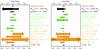 |
Fig. 10 Impact of model parameters on the millimetre SED slope (left) and centimetre SED slope (right), as defined by Eqs. (D.7) and (D.8), respectively. The model parameters which have been varied are listed to the right of each plot (see Table 3 for explanations of the symbols), along with the ranges explored. The colours indicate different groups of model parameters. Gas and dust masses are shown in black, disk shape parameters in green, and dust size, material and settling parameters in orange. The changes of the observable quantity, here e.g. the mm-slope, caused by varying a particular model parameter, are shown with arrows. The original value of the observable quantity is shown by the red point marked with “reference model” (for example, 2.4 for the mm-slope), where the top x-axis provides an absolute scale, and the bottom x-axis provides a relative scale with respect to the value obtained by the reference model. The arrows indicate the direction and magnitude of changes caused. Leftward arrows indicate a flattening of the SED, rightward arrows a steepening. The corresponding parameter values are shown to the left and right of the “–” to the right of each plot. For example, increasing the disk mass Mdisk from the reference value to 0.1 M⊙ results in a flatter SED |


5.3.2. Visibilities
Figure 9 shows the impact of model parameters on the calculated visibilities at 1.6 μm (e.g. PIONIER), at 10 μm (e.g. MIDI), and at 1.3 mm (e.g. CARMA, ALMA). The mm-visibility (see e.g. Guilloteau et al. 2011) probes the apparent spatial extension of the disk, limited by minimum optical depth requirements to produce a detectable signal at those wavelengths. This apparent size is most directly influenced by the tapering-off radius Rtap. The “sharpness” of the outer edge γ is reflected by the steepness of the V2-decline. However, more dust in the outer regions (larger Mdust, smaller ϵ) also increases the optical depths in these regions, which leads to larger apparent sizes as well. Strong dust settling αsettle → 10-4 moves the grains toward the midplane into the disk shadow where they are substantially cooler (see Sect. 5.3.3 and Fig. 7), so cold that some fraction of the dust grains does not emit in the Rayleigh limit at 1.3mm, thus producing less extended flux, which leads to a smaller apparent size5.
The 10 μm visibilities reflect the radial extension of warm dust in the disk surface layer producing the 10 μm silicate emission feature (about 1 AU in the reference model). This extension is larger for warm, e.g. flared disks. In contrast, parameter choices which lead to cooler conditions at 1 AU cause a smaller appearance of the disk at 10 μm. Such parameter choices include smaller scale heights H0, dust size parameter variations that increase the mean dust size (larger amin, smaller apow), and lacking amorphous carbon. Dust settling plays no significant role here.
The 1.6 μm visibilities are more difficult to understand, see (Anthonioz et al. 2015). They have three components: the star, scattering and emission from the inner rim, and extended scattering. The extended scattering leads to a slight tilt of the V2-curves beyond baselines [kλ] ≳ 100, before V2 drops to much lower values at baselines which corresponds to the inner rim of the disk (0.07 AU in the model). At even longer baselines, the interferometer would start to resolve the star (R⋆ = 0.0097 AU), and the visibility would drop sharply, but such long baselines are currently not accessible, and not included in Fig. 9). The 1.6 μm visibilities hence probe the relative contributions of these three components and their spatial extensions. Most remarkably is the influence of flaring and settling, which powers/suppresses the extended scattering component, and the fraction of amorphous carbon which changes the albedo of the dust particles. Pure silicate dust particles (amC = 0), for example, are almost perfect scatterers at 1.6 μm, leading to a much more pronounced extended scattering component.
Noteworthy, the hydrostatic disk models show a stronger extended scattering component as well (because of the strong flaring of the outer disk), and less contributions from the inner rim, which has a lower wall height.
The inner rim radius Rin directly affects the second component of the 1.6 μm visibilities directly, namely the emission and scattering from the inner rim. Large Rin can also limit the radial extension of the 10 μm emission region from the inside, introducing new small scales in form of the ring thickness and the apparent height of the inner rim wall, with sharp edges, which leads to more complex visibility shapes.
5.3.3. The mm-slope and cm-slope
Figure 10 shows the impact of the model parameters on the observable SED slopes at millimetre and centimetre wavelengths, as defined by Eqs. (D.7) and (D.8), which are important diagnostics of grain growth in protoplanetary disks, see e.g. (Natta et al. 2007) and (Testi et al. 2014). The SED slopes are expected to reflect the dust absorption opacity slopes, with some flattening due to optical depth effects  (10)Eq. (10) was derived by Beckwith et al. (1990)6 for a powerlaw surface density structure Σ ∝ r− p and a vertically isothermal powerlaw temperature distribution T ∝ r− q. This formalism was later relaxed by Ricci et al. (2010, 2012), who determined T(r) according to Chiang & Goldreich (1997) and considered a self-similar disk with tapered outer edge. Ricciet al. found values αSED ≈ 1.9−2.7 for the Taurus-Auriga region, which are significantly lower than what is expected from small interstellar grains βabs ≈ 1.7 (Draine 2006), suggesting that the dust in protoplanetary disks must have much smaller βabs ≈ 0.3−1.0 at (1−3) mm, indicating dust growth.
The standard DIANA opacities have  and
and  , thus the SED slopes of the reference model are expected to be
  and
and  in the optically thin limit Δ = 0. However, the reference model exhibits
  and
and  , in agreement with observations, suggesting optical depths corrections of Δmm ≈ 1.5 and Δcm ≈ 0.1, respectively.
Closer inspection shows, however, that these derived Δ do not agree at all with the expected flattening due to optical depth effects. The radius r1 where the vertical dust optical depth equals unity  (11)is only r1 ≈ 6.9 AU at λ = 1.3 mm and r1 = 0.9 AU at λ = 7 mm in the reference model, which results in tiny corrections, Δmm = 0.04−0.12 and Δcm = 0.01−0.03, as derived from the equations in Beckwith et al. (1990), depending on what is assumed for the outer radius in our tapered-edged models. At both wavelengths, the expected Δ-corrections are too small, inconsistent with the results obtained from our radiative transfer models.
This conclusion holds for all models computed in this paper. The strongest optical depth effects occur in massive disks (Mdisk = 0.1 M⊙), if the mass is more concentrated toward the centre (ϵ = 1.5), if the disk is small (Rtap = 50 AU), and/or if the dust size and opacity parameters lead to larger mm-opacities. But even in all these cases, the expected Beckwith et al. Δ-corrections for optical depths effects at 1.3 mm stay well below unity, which is insufficient to explain the gentle mm-slopes obtained from our radiative transfer models. The mm-slopes from the computed SEDs are more gentle than expected, and optical depth effects are not the key to explain these discrepancies7.
Beckwith et al. (1990) derived Eq. (10) by assuming that all dust grains emit in the Rayleigh limit. If we ignore optical depth effects for a moment, the observable flux Fν is exactly given by  (12)where
  is the dust absorption coefficient per dust mass (assumed to be constant throughout the disk),
  is the dust mass averaged Planck function, and Mdust is the total dust mass. The log-log slope αSED = −∂log Fν/∂log λ is then given by
  (13)Table 4 shows that the deviations of the Planck derivative from its limiting value of 2 can be substantial. At 1.3 mm, for example, the Planck slope is about 1.35 and not 2, if the grains emit at 10 K. At 7 mm, deviations ≳0.2 dex are still conceivable if the majority of grains would emit at 5 K. Indeed, using these deviations from Rayleigh-Jeans regime, Dutrey et al. (2014) report on vertical mean dust temperatures of 8.5 K at 300 AU in the disk of GGTau.
Negative logarithmic derivative of the Planck function, −∂log Bν(T) /∂log λ, as function of temperature and wavelength.
The dependencies of αSED on the disk temperature structure, according to Eq. (13), can explain the results obtained from our radiative transfer models. The mean dust temperature according to Eq. (D.2) is ⟨ Tdust ⟩ ≈ 19 K in the reference model, but this is a linear mean, and the Planck function is highly non-linear at low temperatures ⟨ Bν(T) ⟩ ≪ Bν( ⟨ T ⟩). Simply put, a considerable part of the dust in the disk is so cold that it does not contribute significantly to the 1.3 mm flux. The minimum dust temperature in the reference model is about 4.5 K. The cold dust over total dust mass fraction is 0.12 (for Tdust< 7 K), 0.31 (for Tdust< 10 K), 0.58 (for Tdust< 15 K), and 0.75 (for Tdust< 20 K). It is about this fraction, with efficiencies according to Table 4, that is missing in the observable flux, causing the deviations from αSED = 2 + βabs.
These temperature effects explain the qualitative behaviour of the SED millimetre and centimetre slopes in the models as shown in Fig. 10. The dust size and material parameters impact the SED slope directly via changing the dust absorption slope βabs, compare Fig. 3. These parameters have the strongest impact on the SED slope. The green disk shape parameters have an influence on the dust temperature structure in the disk Tdust(r,z) and, therefore, have an indirect influence on the SED slope. Figure 11 shows that all disk shape parameters that lead to very cold midplane conditions in the disk around r ≈ 50 AU are well correlated with the more gentle mm-slopes in the models, in particular little flaring (β = 1.05) and a steep column-density structure (ϵ = 1.5). However, dust settling has in fact an even stronger impact (αsettle = 10-4, leftmost point in Fig. 10). By settling, the bigger grains are moved to the cooler midplane, and concentrating the grains toward the midplane also increases the shadow formation there, making the midplane even cooler.
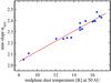 |
Fig. 11 Correlation between computed SED mm-slope (as measured between 850 μm and 1.3 mm) and midplane dust temperature at r = 50 AU for models with identical dust properties and disk mass. Varied parameters include gas/dust (at constant Mdust), Rin, Rtap, ϵ, γ, H(100 AU), β and αsettle, i.e. the green disk shape parameters in Fig. 10 and dust settling. |
Our conclusion is that, indeed, the dust absorption opacity slope βabs mostly determines the SED slope. However, αSED flattens significantly for cold disks, an effect that has not been reported so far and that seems more important that the classical Δ-correction for optical depth effects (Beckwith et al. 1990).
5.3.4. The [OI] 63.2 μm emission line
We now turn our attention from continuum observations to gas emission lines. We have selected four representative emission lines for the discussion in this paper, which are frequently observed, and which emerge from different disk regions, see Fig. 12. All selected lines have chemically robust carriers, namely the O-atom or the CO-molecule, which are not critically dependent on chemical details. These lines are rather influenced by the shape of the disk and gas temperature distribution in the disk surface layer.
The [OI] 63.2 μm line is usually the strongest disk emission line throughout the electromagnetic spectrum, compare Fig. 4, and has been detected in 84% of T Tauri stars with disk dust masses >10-5 M⊙ by the Herschel open time key program GASPS (Dent et al. 2013), including outflow sources (see Howard et al. 2013). With an excitation energy of 227 K and a critical density of ~6 × 105 cm-3, this line originates in disk layers even above the CO containing molecular layers, see Fig. 12. In order to excite this line, the gas needs to be as warm as ≳50 K (Kamp et al. 2010). These conditions are only present in outflows and in the disk up to radial distances ≲100 AU, above the molecular layers which are too cold because of molecular line cooling.
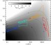 |
Fig. 12 Line emitting regions in the reference model. The surrounded areas are responsible for 50% of the vertically emitted line fluxes as annotated. The black dashed contours show the hydrogen nuclei particle density log n⟨ H ⟩(r,z). The yellow dotted contour line shows the upper boundary of the molecular layer where nCO/n⟨ H ⟩ = 10-5. |
The impact of the model parameters on the predicted [OI] 63.2 μm line flux is shown in Fig. 13. According to the physical excitation mechanism explained in the previous paragraph, the line flux increases with all parameters that directly trigger the heating in the uppermost disk layers, marked in blue in Fig. 13, namely the stellar UV excess fUV, the X-ray luminosity LX, the PAH concentration fPAH and the efficiency of exothermic reactions γchem. The disk shape parameters (marked in green in Fig. 13) also play an important role. For a self-shadowed disk (e.g. for flaring index β = 1.05), the distant oxygen gas is situated in the disk shadow, and the [OI] 63.2 μm line is substantially suppressed. The line is massively optically thick (τline ≈ 100 in the reference model at 100 AU), so what counts is the size of the disk surface area with gas temperatures Tgas ≳ 50 K, which depends on the disk mass and shape parameters Hg(100 AU), β and ϵ. In comparison, dust size parameters and inclination play no significant role for this line.
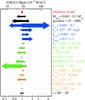 |
Fig. 13 “Impactogram” of the [OI] 63.2 μm emission line. The absolute line flux is depicted on the top abscissa, as well as relative to the reference model at the bottom. Leftward arrows indicate a weakening of the line, and rightward arrows a strengthening of the line, due to changes of single model parameter as indicated on the r.h.s. The colours indicate groups of parameters. Gas and dust masses are shown in black, heating parameters in blue, disk shape parameters in green, and dust parameters in orange. See Fig. 10 for further explanations. |
Figure 13 shows that 5 different model parameters are able to change the [OI] 63.2 μm line flux by at least a factor of 2 within their reasonable ranges of values, therefore, finding clear correlations of the [OI] 63.2 μm line flux with one of these parameters seems quite unlikely, which could explain why Meeus et al. (2012) and Aresu et al. (2014) have reported on negative results concerning such correlations.
Since the [OI] 63.2 μm line is optically thick, one would not expect the gas mass nor the gas/dust ratio to be important. However, for this particular line, there is an interesting energy conservation mechanism at work. The emission of [OI] 63.2 μm line photons is the dominant cooling process in the line emitting regions, and therefore, the line luminosity must roughly equal the integrated heating rate in the [OI] 63.2 μm line emitting volume. Consequently, the gas temperature in this volume can be expected to relax towards an equilibrium value where the [OI] 63.2 μm line cooling balances the total heating, henceforth denoted as “self-regulation mechanism”. The heating in the line emitting region is provided by a number of physical processes that absorb and thermalise fractions of the incoming UV and X-ray photon energies, namely X-ray Coulomb heating, heating by neutral carbon photo-ionisation, PAH heating via photo-effect, and heating by exothermic chemical reactions driven by UV and X-ray reactions. For larger disk masses, the solid angle (as seen from the star) of the distant disk regions that absorb the UV and X-ray photons increases, therefore, the [OI] 63.2 μm line flux increases. The impact of the gas/dust ratio is actually more significant, as there is a competition between dust versus gas absorption of UV photons. For larger gas/dust ratios, fewer UV photons are absorbed by the dust (and re-emitted as continuous far-IR radiation), hence more of the available UV flux is converted into gas heating.
As a consequence of these processes, more gas (less dust) generally leads to an increase of the size of the disk surface area where Tgas ≳ 50 K. More specifically, an increase of the gas mass causes the [OI] 63.2 μm line emission region to shift upwards (Kamp et al. 2010), which captures more of the impinging UV and X-ray photons. However, because of the self-regulating energy conservation mechanisms explained above, effects are rather modest. By varying the gas mass by a factor of 10, the [OI] 63.2 μm line only changes by factors of a few.
5.3.5. CO high-J emission lines
As an example for high-J CO emission lines, we have selected the CO J = 18 → 17 line at 144.8 μm with an excitation energy of 945 K and a critical density of ~2 × 106 cm-3. Due to its high excitation energy, gas temperatures Tgas ≳ 200 K are required to excite this line, and these conditions are only present in the CO surface layer inside of r ≲ 5 AU in the reference model. The line is optically thick, but approaches τline = 1 at the outer boundary of the line emitting region. The line is rather weak in the reference model, a factor of about 30 lower than the Herschel/PACS detection limit. In fact, detection rates of this line for T Tauri stars are rather low, about 41% of the 34 objects selected by GASPS (Dent et al. 2013)8, most of them being identified as outflow sources (see Howard et al. 2013).
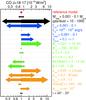 |
Fig. 14 Impact of model parameters on the CO J = 18 → 17 emission line at 144.87 μm, see Fig. 10 for explanations. |
The “impactogram” of the CO J = 18 → 17 line (Fig. 14) shows many similarities to the behaviour of the [OI] 63.2 μm line (Fig. 13), for example the direction of effects, but the scaling of the abscissa is different. We are now reporting on effects that can potentially change a line flux by one order of magnitude.
Since both line and continuum are optically thick, and level populations are close to LTE, we can use Eq. (E.3), see Appendix E, to estimate the line flux. This demonstrates that for these optically thick far-IR lines, it is the difference between gas and dust temperatures (in the disk surface layers between about 1 AU and 5 AU) that determines the line flux.
Besides the parameters directly involved in the gas heating (blue), we can conclude from Fig. 14 that also the dust size parameters play an essential role. All parameter changes that imply an increase of the mean dust particle size (orange) lead to a reduction of the dust UV opacity, see Sect. 5.2.1, and hence to an increase of the thickness of the layer where the gas temperature is substantially larger than the dust temperature. Precisely speaking, as will be explained in Sect. 5.3.7 and Fig. 20, it is the ratio τline/τUV which is important. Since the gas temperature structure is more or less fixed to τUV, more gas, or lower UV continuum optical depths, both result in larger CO J = 18 → 17 line fluxes. This also explains the dependence on dust settling.
Interestingly, when the inner disk radius is increased in the model to 10 AU, i.e. well beyond the outer radius of the line emitting region in the reference model, the line flux increases. In this case, instead of radially continuous line emission, the line is preferentially emitted from the distant inner wall, and the larger emitting area of that wall seems more relevant than the radial dilution of the impinging UV and X-ray photons, as long as this high-energy irradiation is sufficient to cause gas temperatures ≳200 K at the inner wall.
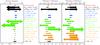 |
Fig. 15 Predicted behaviour of the 12CO, 13CO and C18O J = 2 → 1 isotopologue lines around 1.3 mm. The left plot shows the impact of model parameters on the predicted 12CO line flux, see Fig. 10 for more explanations. The two figures on the right show the impacts of model parameters on the 12CO /13CO and 13CO/C18O line ratios. Note that the direction of effects is sometimes inversed on the r.h.s., for example the dependency on disk flaring parameter β. Less flaring leeds to weaker CO lines in general, but to larger line ratios. On the right, both an increase and a decrease of the amorphous carbon dust volume fraction Vol(AC) lead to higher line ratios, here the larger arrows correspond to Vol(AC) = 0%. |
5.3.6. (sub-)mm CO isotopologue lines
The CO J = 2 → 1 isotopologue lines have excitation energies of about 17 K and critical densities ~7 × 104 cm-3. The impact of the model parameters on our computed CO isotopologue line fluxes is shown in Fig. 15. In the following, we discuss these results obtained by our 3D diagnostic line transfer computations (Sect. 3.10), by means of a few simplified equations, to demonstrate and understand the main dependencies we find. The 12CO line is optically thick in all models, the 13CO is optically thick in most models, and the C18O line is borderline optically thin, meaning that the radial distances R(τline = 1), up to which the lines are optically thick, depends on isotopologue. In the reference model, R(τline = 1) ≈ 450 AU for the 12CO line, ≈210 AU for the 13CO line, and ≈110 AU for the C18O line. The level populations connected to the CO isotopologue lines in the (sub-)mm regime result to be close to LTE, and the continuum is optically thin. Under these circumstances, the line fluxes are approximately given by ![\begin{equation} F_{\rm line} \approx 2\Delta\Omega\,\Delta\nu\, B_\nu[T_{\rm gas}(\tau_{\rm line}=1)] , \label{eq:lineapprox} \end{equation}](/articles/aa/full_html/2016/02/aa26538-15/aa26538-15-eq347.png) (14)see Eq. (E.2) and explanations in Appendix E. The mean gas temperature in the CO (sub-)mm line emission regions (see Fig. 12) results to be ⟨ Tgas ⟩ ≈ Tgas(τline = 1) ≈ 20−35 K, and varies only little throughout the presented models (all isotopologues). This temperature only affects the line fluxes in a linear way in the Rayleigh-Jeans limit. Therefore, the discussion of the CO isotopologue line fluxes
(14)see Eq. (E.2) and explanations in Appendix E. The mean gas temperature in the CO (sub-)mm line emission regions (see Fig. 12) results to be ⟨ Tgas ⟩ ≈ Tgas(τline = 1) ≈ 20−35 K, and varies only little throughout the presented models (all isotopologues). This temperature only affects the line fluxes in a linear way in the Rayleigh-Jeans limit. Therefore, the discussion of the CO isotopologue line fluxes 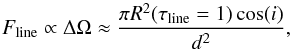 (15)simplifies to a discussion of the radius up to which the CO lines are optically thick R(τline = 1) as follows.
-
The 12CO line fluxes depend only little on all parameters which do not change R(τline = 1) significantly, in particular fUV, LX, fPAH, dust size and settling parameters, scale height H0 and flaring parameter β, as well as parameters only relevant for the inner disk, such as Rin.
-
Most important are those model parameters which directly determine R(τline = 1), these are the tapering-off radius Rtap and the tapering-off exponent γ.
-
The dependency on γ is remarkable. The reference model has a tapering-off radius of Rtap = 100 AU, a mean CO emission temperature of Tgas(τline = 1) ≈ 25 K, and a 12CO J = 2 → 1 line flux of 15.7 Jy km s-1 (1.2 × 10⁻¹⁹ W/m2). According to Eq. (14), this line flux corresponds to an emitting radius of R(τline = 1) = 450 AU, which is possible only because we assume a smoothly decreasing surface density structure beyond Rtap with γ = 1 in the reference model. If the disk has a much sharper outer edge (γ = −0.5) the mean CO emission temperature increases by 10 K, but the flux is down to 4.2 Jy km s-1 (3.3 × 10⁻²⁰ W/m2), which then corresponds to a radius of only 200 AU. These numbers are in very good agreement with the radii R(τline = 1) that we can directly measure in the models, see Fig. 12.
There are a number of model parameters which indirectly change R(τline = 1), among them the disk mass Mdisk, the gas/dust ratio, and the column density powerlaw exponent ϵ. These parameters change the amount of CO gas in the outer regions, which implies that R(τline = 1) changes, too. These indirect influences on the CO line fluxes are stronger in models with exponential tapering-off. Models with a sharp outer edge do not show much of those effects.
To summarise, the 12CO (sub-)mm lines probe the conditions in the tapering-off distant gas above and around the disk, well beyond the radial zones emitting the continuum. These conclusions are robust, almost purely geometrical, because CO is such an abundant and robust chemical constituent of the disks. There is no need for any sophisticated chemical effects to understand these lines.
In contrast, the CO isotopologue line ratios (see r.h.s. of Fig. 15) are more difficult to understand. It has been suggested, e.g. by Williams & Best (2014) and Miotello et al. (2014), that the CO isotopologue line ratios are an excellent probe of the disk mass, in particular if rare isotopes like C18O and C17O can be observed with high sensitivity9. We see the dependence of isotopologue line ratios on disk mass clearly in our models, too, but we also see other parameter dependencies that can be equally important. When looking at line ratios, the major dependencies (like Fline ∝ R2) cancel, though not completely, and other secondary temperature and chemical effects come into play. The (sub-)mm CO isotopologue line ratios show the following effects:
-
The dependence of the 12CO /13CO line ratio on disk mass is almost negligible in our models, consistent with Williams & Best (2014), because both lines are optically thick. The dependence of the 13CO/C18O line ratio on Mdisk is more pronounced, because the C18O line is borderline optically thin.
-
The asymmetric dependence of the 13CO/C18O line ratio on Mdisk indicates that we need disk masses as low as 10-3 M⊙ to fully be in the optically thin limiting case for the C18O line (the 13CO line is optically thick in most models anyway), also evident from the missing dependence on inclination.
-
The impact of the sharpness of the outer disk edge γ is remarkable. For a very sharp outer edge (γ = −0.5) we come close to a configuration where all three CO isotopologue lines remain optically thick until the disk ends abruptly, see Fig. 16, in which case the line ratios would be unity. However, there are secondary temperature-effects (the 13CO and C18O lines are emitted from deeper layers which are cooler) which always keep the isotopologue line ratios >1.
-
The dependencies on the gas/dust ratio are much more pronounced than on Mdisk, which shows that it is not simply the gas mass that counts. In fact, the two models denoted by Mdisk = 0.001 M⊙ and gas/dust = 10 have the same gas mass, they only differ in terms of their total dust mass (see footnote below Table 3). The more dusty model (gas/dust = 10) has a taller midplane shadow, hence cooler conditions even at higher disk layers, and more CO ice. Therefore, the 13CO line becomes borderline optically thin and its flux drops quickly, leading to a larger 12CO /13CO line ratio.
-
Figure 15 shows a strong impact of disk flaring (parameter β) on the CO isotopologue line ratios, which again can be attributed to CO ice formation. The β = 1.05 model produces a self-shadowed disk configuration with very cold midplane conditions, favouring CO ice formation. The resulting lower gaseous CO column densities weaken in particular the 13CO line, hence the 12CO /13CO line ratio becomes larger.
-
There are also noticeable dependencies on dust size parameters and dust settling, which are again related to CO ice formation. All dust size and opacity parameters which lead to an increase of the dust opacities around 1 μm lead to a more pronounced midplane shadow, cooler conditions around (100−300) AU, more CO ice, hence larger 12CO /13CO line ratios.
To summarise, the analysis of the (sub-)mm CO isotopologue line ratios requires sophisticated modelling where the sharpness of the outer disk edge, the strength and thickness of the disk midplane shadow impacting the CO ice formation, and vertical temperature effects all play a significant role. Spatially resolved line data with high S/N (e.g. ALMA) are required to disentangle these effects.
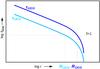 |
Fig. 16 Understanding (sub-)mm CO isotopologue line ratios. The 13CO line is weaker, because it approaches τline = 1 at smaller radii. Similar apparent radii (and fluxes) of the 12CO and 13CO lines can be obtained by making the outer disk edge sharp. |
5.3.7. CO υ = 1 → 0 emission lines
The fundamental ro-vibrational CO υ = 1 → 0 emission lines are regularly detected in T Tauri stars (e.g. Najita et al. 2003; Salyk et al. 2011; Brown et al. 2013), in Herbig Ae/Be stars (Brittain et al. 2003; Blake & Boogert 2004; van der Plas et al. 2015), as well as in transition disks (Goto et al. 2006; Salyk et al. 2009; Pontoppidan et al. 2008). Surveys of CO ro-vibrational emission lines in young stars (e.g. Brown et al. 2013) detect 12CO emission in about ~80% of the objects. The line profiles are generally double-peaked, but, in many objects, in particular in T Tauri stars, line profiles can also be singly peaked which is usually interpreted in terms of a slow (few km/s) molecular disk wind (Pontoppidan et al. 2011; Bast et al. 2011; Brown et al. 2013). 12CO integrated line fluxes observed are of order 10-17 W/m2, and line widths are 12−200 km s-1, mostly reflecting the expected distribution of inclination. Disks around early-type Herbig AeBe stars have narrower line profiles, on average, than T Tauri stars Brown et al. (2013).
The lines have excitation energies (3000−6000) K and critical densities10 of order (1012−1014 ) cm-3, depending on temperature and depending on whether the gas is H2-rich or atomic, see (Thi et al. 2013) for details. The low-J fundamental CO lines are always massively optically thick in our models, with vertical line centre optical depths of order 104−107 for r< 10 AU in the reference model. Figure 12 shows that the CO υ = 1 → 0 lines are vertically emitted by a region that extends radially to about 1 AU in the reference model, from a thin horizontal layer at the top of the warm molecular layer. In addition, the line can also be emitted from the far side of the directly illuminated inner rim, if the disk is seen under an inclination angle i> 0°. This contribution is not accounted for in Fig. 12, and may in fact domiante under certain circumstances.
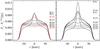 |
Fig. 17 CO υ = 1 → 0 line velocity profiles predicted by the reference model, continuum subtracted and convolved with a 12 km s-1 Gaussian (resolution R ≈ 25 000). The R(10) and R(35) lines plotted in red are selected for further study of the model parameters impacts in Fig. 18. |
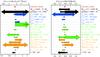 |
Fig. 18 Impact of model parameters on ro-vibrational CO emission. On the l.h.s, the υ = 1 → 0R(10) line has been selected to study the effects of changing model parameters on line flux. The r.h.s. shows the R(35) /R(10) line ratio, a measure for the “CO rotational excitation temperature”. Large line ratios indicate emission from hot CO. Note that the direction of parameter impact is often reversed on the r.h.s., i.e. weak lines are usually emitted from a tiny area of hot gas, whereas strong lines are emitted from an extended area of cool gas. See Fig. 10 for further explanations. |
In LTE, the CO gas will emit substantially in the fundamental lines if (i) the gas temperatures exceed about 500−1000 K; and (ii) the gas is significantly warmer than the local dust temperature, according to Eq. (E.3) in Appendix E![\begin{equation} F_{\rm line} \approx 2 \Delta\Omega\,\Delta\nu \left(B_\nu[T_{\rm gas}(\tau_{\rm line}=1)] -B_\nu[T_{\rm dust}(\tau_{\rm cont}=1)]\right) . \end{equation}](/articles/aa/full_html/2016/02/aa26538-15/aa26538-15-eq377.png) (16)These two conditions are always fulfilled at the inner rim, or, more precisely speaking, in the thin hot surface layer that covers the inner rim facing the star, which forms a very thin radial photodissociation region (PDR). These emissions from the inner rim creates a broad, box-like “minimum CO emission profile” for all R-branch and P-branch lines (Fig. 17) with a hot characteristic emission temperature. However, the CO emission lines created this way would be quite faint and could not be detected with current instruments, because of the tiny solid angle ΔΩ occupied by the inner rims of T Tauri stars.
(16)These two conditions are always fulfilled at the inner rim, or, more precisely speaking, in the thin hot surface layer that covers the inner rim facing the star, which forms a very thin radial photodissociation region (PDR). These emissions from the inner rim creates a broad, box-like “minimum CO emission profile” for all R-branch and P-branch lines (Fig. 17) with a hot characteristic emission temperature. However, the CO emission lines created this way would be quite faint and could not be detected with current instruments, because of the tiny solid angle ΔΩ occupied by the inner rims of T Tauri stars.
In order to create observable line fluxes, the model must fulfil the above stated two conditions for CO υ = 1 → 0 emission also at larger radii, which only occurs in some models, depending on the parameters important for the gas heating, flaring, and dust shielding (Figs. 18 and G.1). If the extended gas is sufficiently warm, we have a mixture of narrow (extended) cool CO emission with some broad, hot emission from the inner rim, (Fig. 17). The emissions from the extended regions are lacking strong high-J lines not only because the gas is cooler there, but also because the optical depths are smaller for the high-J lines, i.e. the high-J lines probe deeper layers which are cooler, and where the differences between gas and dust temperatures start to vanish (Fig. 20). The cool, extended contributions add a central component to the line profile which is often double-peaked, but not always (Fig. G.1).
The following results have been obtained with the default CO model molecule in ProDiMo with vibrational quantum numbers v ≤ 2 and rotational quantum numbers J ≤ 50, limited to 110 levels, see (Thi et al. 2013) for extended options. Figure 18 shows the impact of the model parameters on the R(10) line flux and characteristic CO emission temperature as measured by R(35)/R(10). Figure G.1 shows how the mean line profile changes when selected model parameters are varied. The main effects are as follows.
-
Stronger CO line fluxes are connected with more centrally peaked line emissions coming from larger emitting areas.
-
All parameters that increase gas heating will generally increase line flux, in particular the UV excess fUV (Garufi et al. 2014) and the efficiency of chemical heating γchem.
-
However, the X-ray luminosity has no significant influence on the fundamental CO emission lines.
-
Disk flaring makes the CO lines stronger and cooler.
-
A larger inner disk radius Rin leads to a larger solid angle
 , hence substantially stronger CO lines. If Rin is increased, the heating UV flux gets radially diluted ∝
 , but can still provide sufficient gas heating and CO excitation up to about Rin ~ 3 AU, depending on stellar UV luminosity. For even larger Rin, however, the excitation conditions for fundamental CO line emission break down, see Fig. 19.
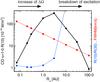
Fig. 19 Impact of inner disk radius Rin on CO υ = 1 → 0 line emission fluxes and FWHM. The black line shows the computed R(10) line fluxes for the reference model, when varying Rin between 0.07 AU and 100 AU. The blue line shows the R(10) /R(35) line ratio, and the red line shows the computed R(10) line widths.
-
There is a strong impact of the dust size parameters on the CO fundamental line emission. This is due to changes in the dust UV optical depths τUV, see Fig. 20. Dust parameter choices which favour larger particles (larger amin, larger amax, smaller apow) and less amorphous carbon reduce the UV dust opacities, i.e. the UV light can penetrate deeper into the CO line emitting regions, which increases the gas temperatures and CO line fluxes.
-
After the inner disk radius, the gas/dust ratio has the largest impact on the fundamental CO emission. The reason for this effect is the same as for the dust size parameters. Larger gas/dust ratios lead to an increase of the τline/τUV ratio.
To summarise, the impinging UV flux and the local τline/τUV ratio regulate the strength of the CO fundamental line emissions, but the disk shape determines how much of the stellar UV flux reaches a disk region under consideration. The reference model shows very weak CO fundamental line fluxes with broad, box-like profiles, which would in fact lead to non-detections, but the model parameters can be changed to result in observable line flux levels and more typical CO line profiles.
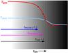 |
Fig. 20 Understanding optically thick CO ro-vibrational emission lines. The sketch can either represent the inner rim horizontally, or a distant disk column vertically. The gas and dust temperature structure is connected to τUV, the dust optical depth in the UV. High-J and low-J CO emission lines have different line optical depths, so their fluxes probe the contrast between gas and dust temperatures at different depths. |
The strong dependence of the CO υ = 1 → 0 line fluxes on Rin suggests that any disk shape irregularities in the inner regions ≲30 AU, which create highly extended vertical gas columns that are exposed to fresh UV light from the central star, could easily dominate the CO fundamental emission lines. Such irregularities could be, for example, (i) large inner holes; (ii) disk gaps with highly puffed-up secondary inner walls; (iii) spiral waves which are warmer than the surrounding gas, causing those regions to stick out vertically; or (iv) the launching regions of disk winds.
6. Summary and conclusions
The analysis and interpretation of observational data from Class II and III protoplanetary disks is a challenging task. Various hydrodynamical, chemical, dust, and radiative processes are coupled to each other in complicated ways, and current disk modelling groups are using quite different assumptions to setup their 2D radiative transfer and thermo-chemical models concerning disk shape, dust size and opacity parameters, treatment of PAHs, and dust settling.
We have systematically investigated the effects of those assumptions in this paper by have studying the impact of the associated model parameters on the various continuum and line predictions, using a holistic disk modelling approach which allows us to calculate all continuum and line observations on the basis of a single model. The most important effects are:
-
Disk shape matters. In particular, scale heights and disk flaringhave large impacts on the gas and dust temperature distribution inthe disk, and hence on SED, visibilities and gas emission lines. Forvery cold, self-shadowed disk configurations, ice formation canstrongly reduce the (sub-mm) emission lines.
-
Hydrostatic T Tauri disk models produce only little near-IR excess, but a strong flaring of the outer disk, which leads to a re-increase of the spectral flux νFν between λ = (20−50) μm, whereas the opposite is typically observed for non-transitional disk.
-
Dust size is important, not only for modelling the continuum, but also for modelling chemistry and emission lines, which is often not discussed in thermo-chemical disk models. By extending the dust size distribution to mm sizes, as required to fit the SED, the UV dust opacity is reduced by a factor of about 100, which means that UV photons can penetrate much deeper into the disk with ample effects on chemistry, temperature structure and gas emission lines.
-
New dust standard opacities have been developed. Guided by a study of the multi-wavelength optical properties of dust aggregates particles (Min et al. 2016), we have developed a simplified and fast numerical treatment for dust opacities. We propose to use an effective porous mixture of amorphous laboratory silicates with amorphous carbon, a powerlaw size distribution with a distribution of hollow spheres to capture the most important size, material, and shape effects. A Fortran-90 package to compute the DIANA standard dust opacities11.
-
Disk flaring and/or dust settling? Dust settling affects primarily the outer disk regions, leading to cooler disks, lower continuum fluxes at mid-IR to cm wavelengths, and smaller apparent disk sizes in the millimetre continuum. These effects on the continuum observables are very similar to those in models with little or lacking disk flaring. However, concerning the gas emission lines, dust settling has just the opposite effect. Dust settling leaves the vertically extended gas bare and exposed to the stellar UV radiation, leading to higher gas temperatures and stronger gas emission lines in general. Thus, we can expect to distinguish between disk flaring and dust settling by observing in particular far-IR emission lines.
-
PAHs can have important effects on the disk radiative transfer, even if the mid-IR PAH features are not visible in the SED. If the PAH abundance reaches about 10% of the interstellar standard, the PAH opacities start to catch up with the dust opacities in the UV and blue parts of the spectrum. Since the PAHs are not settled, and have negligible scattering opacities, the PAHs change the ways in which UV photons reach the disk. In fact, the PAHs can effectively “shield” the disk from UV photons. We are proposing a simplified method by treating the PAHs consistently in the continuum radiative transfer assuming radiative equilibrium, with a PAH temperature independent from the dust temperature.
With regard to particular observations, we find the following robust dependencies that can be used for diagnostic purposes.
-
The SED mm-slope is more gentle than expected from the dustopacity-slope if the disk is cold in the midplane, which happensconsistently in all of our T Tauri models.
-
The [OI] 63.2 μm line is optically thick under all explored circumstances, and probes the tenuous layers above the molecular disk at radii ~(10−100) AU. Since this line provides the most important cooling process in these layers, it is subject to a self-regulation mechanism where the line luminosity must equal the spatially integrated heating rate in that region, in form of various UV and X-ray processes.
-
The high-J CO lines are optically thick and triggered by an excess of the gas temperature over the local dust temperature at the upper edge of the molecular layer around 1−10 AU. The lines are stronger for larger τline/τUV ratios, and hence an excellent tracer of the gas/dust ratio.
-
The (sub-)mm 12CO lines probe the radial extension and conditions in the tapering-off distant gas around the disk, well beyond the radial zones responsible for the (sub-)mm continuum. These conclusions are robust, almost purely geometrical, because these lines are always optically thick in our models, and because CO is such an abundant and chemically robust constituent of the disks.
-
The (sub-)mm CO isotopologue lines of 13CO and C18O require more sophisticated modelling, where the sharpness of the outer disk edge, the strength and vertical extension of the disk midplane shadow, and vertical temperature gradients all play a significant role. The 12CO/13CO isotopologue line ratio is quite independent from disk mass, because both lines are usually optically thick in our models, but increases significantly in cold disks where the increased efficiency of CO ice formation affetcs the 13CO lines more than the 12CO lines.
-
The CO υ = 1−0 fundamental lines are massively optically thick in all our models, and hence provide a clear diagnostic for the existence of warm (≳500 K) gas in the inner disk regions, with a gas temperature in clear excess to the underlying dust temperature. In our standard T Tauri disk setup, these lines are quite weak, because these conditions are mostly met just at the inner rim. Stronger and more extended CO emission lines are obtained, however, if the impinging UV flux is larger, and/or if the local optical depth ratio τline/τUV is larger. In practise, such extended emission occurs in models where sub-micron grains are missing, and/or where the gas/dust ratio is larger, leading to more realistic line profiles. Disk shape irregularities, like inner holes with diameters of order several AU, can lead to much stronger CO fundamental line emissions as well.
Our results demonstrate that the various continuum and line observables probe the physical conditions at very different radii and different heights in the disk. Thus, only a combination of suitable multi-wavelength dust and gas observations can break the various degeneracies, for example those in SED modelling, and can lead to more reliable disk diagnosis.
This paper series aims at setting new disk modelling standards for the analysis of multi-wavelength continuum and line observations for protoplanetary disks, with easy to implement, yet physically grounded, and practical assumptions, which are sufficiently motivated by observations. We will continue this series by exploring the effects of chemical networks and rates in Paper II (Kamp et al., in prep.) and element abundances in Paper III (Rab et al. 2015).
We intend to offer our modelling tools and collected data sets to the community at the end of the FP7 DIANA project12.
This critical opacity value traces back to Beckwith et al. (1990) who proposed ≈10 cm2/g(dust) at 300 µm (1000 GHz).
Available at http://www.diana-project.com/data-results-downloads
Woitke et al. (2013) and Piétu et al. (2014) have reported on the detection of very small protoplanetary disks which could represent a non-negligible fraction of protoplanetary disks in general. These disks are likely optically thick, where this statement is probably not valid.
There was a clear selection bias in (Dent et al. 2013), because only objects with bright [OI] 63.2 μm line were selected for the CO observations, included T Tauri stars with outflows.
CO isotopologue chemistry is not included in our models, we use fixed abundance ratios as 12CO /13CO = 71.4 and 12CO/C18O = 498.7. See Miotello et al. (2014) for the effects of isotope-selective photo-destruction of carbon monoxide.
The large optical depths in the CO fundamental lines tend to “quench” non-LTE effects, so the effective critical density is actually lower by about another 2 orders of magnitude (see, e.g. Woitke et al. 1996).
Available at http://www.diana-project.com/data-results-downloads
Acknowledgments
We would like to thank Dr. Pieter Degroote for compiling a database of updated UV to far-IR photometric measurements for all our 80 targets, including accurate filter functions and zero-points, and Dr. Hein Bertelsen for improving the discussion about fundamental CO emission. The research leading to these results has received funding from the European Union Seventh Framework Programme FP7-2011 under grant agreement no 284405. C. Rab and C. Baldovin-Saavedra acknowledge funding by the Austrian Science Fund (FWF), project number P24790, and the Austrian Research Promotion Agency (FFG) under grant agreement FA 538022, respectively. A. Carmona acknowledge support by the Momentum grant of the MTA CSFK Lendület Disk Research Group. The computer simulations were carried out on the UK MHD Consortium parallel computer at the University of St Andrews, funded jointly by STFC and SRIF.
References
- Akimkin, V., Zhukovska, S., Wiebe, D., et al. 2013, ApJ, 766, 8 [NASA ADS] [CrossRef] [Google Scholar]
- Alexander, R. D., Clarke, C. J., & Pringle, J. E. 2006, MNRAS, 369, 229 [NASA ADS] [CrossRef] [Google Scholar]
- Andrews, S. M., & Williams, J. P. 2005, ApJ, 631, 1134 [NASA ADS] [CrossRef] [Google Scholar]
- Andrews, S. M., Wilner, D. J., Espaillat, C., et al. 2011, ApJ, 732, 42 [NASA ADS] [CrossRef] [Google Scholar]
- Andrews, S. M., Wilner, D. J., Hughes, A. M., et al. 2012, ApJ, 744, 162 [NASA ADS] [CrossRef] [Google Scholar]
- Anthonioz, F., Ménard, F., Pinte, C., et al. 2015, A&A, 574, A41 [NASA ADS] [CrossRef] [EDP Sciences] [Google Scholar]
- Aresu, G., Kamp, I., Meijerink, R., et al. 2011, A&A, 526, A163 [NASA ADS] [CrossRef] [EDP Sciences] [Google Scholar]
- Aresu, G., Kamp, I., Meijerink, R., et al. 2014, A&A, 566, A14 [NASA ADS] [CrossRef] [EDP Sciences] [Google Scholar]
- Arnaud, K. A. 1996, in Astronomical Data Analysis Software and Systems V, eds. G. H. Jacoby, & J. Barnes, ASP Conf. Ser., 101, 17 [Google Scholar]
- Bast, J. E., Brown, J. M., Herczeg, G. J., van Dishoeck, E. F., & Pontoppidan, K. M. 2011, A&A, 527, A119 [NASA ADS] [CrossRef] [EDP Sciences] [Google Scholar]
- Bauschlicher Jr., C., & Bakes, E. 2000, Chem. Phys., 262, 285 [NASA ADS] [CrossRef] [Google Scholar]
- Beckwith, S. V. W., Sargent, A. I., Chini, R. S., & Guesten, R. 1990, AJ, 99, 924 [NASA ADS] [CrossRef] [Google Scholar]
- Bethell, T. J., & Bergin, E. A. 2011, ApJ, 739, 78 [NASA ADS] [CrossRef] [Google Scholar]
- Birnstiel, T., & Andrews, S. M. 2014, ApJ, 780, 153 [NASA ADS] [CrossRef] [Google Scholar]
- Birnstiel, T., Dullemond, C. P., & Brauer, F. 2010, A&A, 513, A79 [NASA ADS] [CrossRef] [EDP Sciences] [Google Scholar]
- Blake, G. A., & Boogert, A. C. A. 2004, ApJ, 606, L73 [NASA ADS] [CrossRef] [Google Scholar]
- Bouy, H., Huélamo, N., Pinte, C., et al. 2008, A&A, 486, 877 [NASA ADS] [CrossRef] [EDP Sciences] [Google Scholar]
- Brittain, S. D., Rettig, T. W., Simon, T., et al. 2003, ApJ, 588, 535 [NASA ADS] [CrossRef] [Google Scholar]
- Brott, I., & Hauschildt, P. H. 2005, in The Three-Dimensional Universe with Gaia, eds. C. Turon, K. S. O’Flaherty, & M. A. C. Perryman, ESA SP, 576, 565 [Google Scholar]
- Brown, J. M., Pontoppidan, K. M., van Dishoeck, E. F., et al. 2013, ApJ, 770, 94 [NASA ADS] [CrossRef] [Google Scholar]
- Bruderer, S. 2013, A&A, 559, A46 [NASA ADS] [CrossRef] [EDP Sciences] [Google Scholar]
- Bruderer, S., van der Marel, N., van Dishoeck, E. F., & van Kempen, T. A. 2014, A&A, 562, A26 [NASA ADS] [CrossRef] [EDP Sciences] [Google Scholar]
- Bruggeman, D. A. G. 1935, Ann. Phys., 416, 636 [NASA ADS] [CrossRef] [Google Scholar]
- Carmona, A., Pinte, C., Thi, W. F., et al. 2014, A&A, 567, A51 [NASA ADS] [CrossRef] [EDP Sciences] [Google Scholar]
- Chiang, E. I., & Goldreich, P. 1997, ApJ, 490, 368 [NASA ADS] [CrossRef] [Google Scholar]
- D’Alessio, P., Canto, J., Calvet, N., & Lizano, S. 1998, ApJ, 500, 411 [NASA ADS] [CrossRef] [Google Scholar]
- de Gregorio-Monsalvo, I., Ménard, F., Dent, W., et al. 2013, A&A, 557, A133 [NASA ADS] [CrossRef] [EDP Sciences] [Google Scholar]
- Dent, W. R. F., Thi, W. F., Kamp, I., et al. 2013, PASP, 125, 477 [NASA ADS] [CrossRef] [Google Scholar]
- Desert, F. X., Boulanger, F., & Shore, S. N. 1986, A&A, 160, 295 [NASA ADS] [Google Scholar]
- DeWarf, L. E., Sepinsky, J. F., Guinan, E. F., Ribas, I., & Nadalin, I. 2003, ApJ, 590, 357 [NASA ADS] [CrossRef] [EDP Sciences] [Google Scholar]
- Dorschner, J., Begemann, B., Henning, T., Jaeger, C., & Mutschke, H. 1995, A&A, 300, 503 [NASA ADS] [Google Scholar]
- Draine, B. T. 2006, ApJ, 636, 1114 [NASA ADS] [CrossRef] [Google Scholar]
- Draine, B. T., & Bertoldi, F. 1996, ApJ, 468, 269 [NASA ADS] [CrossRef] [EDP Sciences] [Google Scholar]
- Draine, B. T., & Lee, H. M. 1984, ApJ, 285, 89 [Google Scholar]
- Draine, B. T., & Li, A. 2007, ApJ, 657, 810 [NASA ADS] [CrossRef] [Google Scholar]
- Du, F., & Bergin, E. A. 2014, ApJ, 792, 2 [NASA ADS] [CrossRef] [Google Scholar]
- Dubrulle, B., Morfill, G., & Sterzik, M. 1995, Icarus, 114, 237 [NASA ADS] [CrossRef] [Google Scholar]
- Dullemond, C. P., & Dominik, C. 2004a, A&A, 417, 159 [NASA ADS] [CrossRef] [EDP Sciences] [Google Scholar]
- Dullemond, C. P., & Dominik, C. 2004b, A&A, 421, 1075 [NASA ADS] [CrossRef] [EDP Sciences] [Google Scholar]
- Dutrey, A., Wakelam, V., Boehler, Y., et al. 2011, A&A, 535, A104 [NASA ADS] [CrossRef] [EDP Sciences] [Google Scholar]
- Dutrey, A., di Folco, E., Guilloteau, S., et al. 2014, Nature, 514, 600 [NASA ADS] [CrossRef] [Google Scholar]
- Espaillat, C., Muzerolle, J., Najita, J., et al. 2014, in Protostars and Planets VI, eds. H. Beuther, et al. (Tucson: University of Arizona Press), 497 [Google Scholar]
- Font, A. S., McCarthy, I. G., Johnstone, D., & Ballantyne, D. R. 2004, ApJ, 607, 890 [NASA ADS] [CrossRef] [Google Scholar]
- Forrest, W. J., Sargent, B., Furlan, E., et al. 2004, ApJS, 154, 443 [NASA ADS] [CrossRef] [Google Scholar]
- Garufi, A., Podio, L., Kamp, I., et al. 2014, A&A, 567, A141 [NASA ADS] [CrossRef] [EDP Sciences] [Google Scholar]
- Geers, V. C., Augereau, J.-C., Pontoppidan, K. M., et al. 2006, A&A, 459, 545 [NASA ADS] [CrossRef] [EDP Sciences] [Google Scholar]
- Gorti, U., & Hollenbach, D. 2008, ApJ, 683, 287 [NASA ADS] [CrossRef] [Google Scholar]
- Gorti, U., & Hollenbach, D. 2009, ApJ, 690, 1539 [Google Scholar]
- Goto, M., Usuda, T., Dullemond, C. P., et al. 2006, ApJ, 652, 758 [NASA ADS] [CrossRef] [Google Scholar]
- Güdel, M., Briggs, K. R., Arzner, K., et al. 2007, A&A, 468, 353 [NASA ADS] [CrossRef] [EDP Sciences] [Google Scholar]
- Guhathakurta, P., & Draine, B. T. 1989, ApJ, 345, 230 [NASA ADS] [CrossRef] [Google Scholar]
- Guilloteau, S., Dutrey, A., Piétu, V., & Boehler, Y. 2011, A&A, 529, A105 [NASA ADS] [CrossRef] [EDP Sciences] [Google Scholar]
- Harries, T. J., Monnier, J. D., Symington, N. H., & Kurosawa, R. 2004, MNRAS, 350, 565 [NASA ADS] [CrossRef] [Google Scholar]
- Hartmann, L., Calvet, N., Gullbring, E., & D’Alessio, P. 1998, ApJ, 495, 385 [NASA ADS] [CrossRef] [Google Scholar]
- Helling, C., Woitke, P., Rimmer, P. B., et al. 2014, Life, 4, 142 [NASA ADS] [CrossRef] [Google Scholar]
- Henning, T., & Semenov, D. 2013, Chem. Rev., 113, 9016 [Google Scholar]
- Hersant, F., Wakelam, V., Dutrey, A., Guilloteau, S., & Herbst, E. 2009, A&A, 493, L49 [NASA ADS] [CrossRef] [EDP Sciences] [Google Scholar]
- Howard, C. D., Sandell, G., Vacca, W. D., et al. 2013, ApJ, 776, 21 [NASA ADS] [CrossRef] [Google Scholar]
- Isella, A., Testi, L., Natta, A., et al. 2007, A&A, 469, 213 [CrossRef] [EDP Sciences] [Google Scholar]
- Jansen, F., Lumb, D., Altieri, B., et al. 2001, A&A, 365, L1 [NASA ADS] [CrossRef] [EDP Sciences] [Google Scholar]
- Kamp, I., Tilling, I., Woitke, P., Thi, W., & Hogerheijde, M. 2010, A&A, 510, A18 [NASA ADS] [CrossRef] [EDP Sciences] [Google Scholar]
- Kraus, S., Ireland, M., Sitko, M., et al. 2013, in Protostars and Planets VI Posters, 51 [Google Scholar]
- Laor, A., & Draine, B. T. 1993, ApJ, 402, 441 [NASA ADS] [CrossRef] [Google Scholar]
- Lefèvre, C., Pagani, L., Juvela, M., et al. 2014, A&A, 572, A20 [NASA ADS] [CrossRef] [EDP Sciences] [Google Scholar]
- Li, A., & Draine, B. T. 2001, ApJ, 554, 778 [Google Scholar]
- Li, A., & Mann, I. 2012, in Nanodust in the Solar System: Discoveries and Interpretations, Astrophys. Space Sci. Libr., eds. I. Mann, N. Meyer-Vernet, & A. Czechowski (Berlin, Heidelberg: Springer), 385, 5 [Google Scholar]
- Lin, D. N. C., & Papaloizou, J. 1986, ApJ, 309, 846 [NASA ADS] [CrossRef] [Google Scholar]
- Maaskant, K. M., Min, M., Waters, L. B. F. M., & Tielens, A. G. G. M. 2014, A&A, 563, A78 [NASA ADS] [CrossRef] [EDP Sciences] [Google Scholar]
- Manske, V., & Henning, T. 1998, A&A, 337, 85 [NASA ADS] [Google Scholar]
- Mathews, G. S., Klaassen, P. D., Juhász, A., et al. 2013, A&A, 557, A132 [NASA ADS] [CrossRef] [EDP Sciences] [Google Scholar]
- Mathis, J. S., Rumpl, W., & Nordsieck, K. H. 1977, ApJ, 217, 425 [NASA ADS] [CrossRef] [Google Scholar]
- Mathis, J. S., Mezger, P. G., & Panagia, N. 1983, A&A, 128, 212 [NASA ADS] [Google Scholar]
- McElroy, D., Walsh, C., Markwick, A. J., et al. 2013, A&A, 550, A36 [NASA ADS] [CrossRef] [EDP Sciences] [Google Scholar]
- Meeus, G., Montesinos, B., Mendigutía, I., et al. 2012, A&A, 544, A78 [NASA ADS] [CrossRef] [EDP Sciences] [Google Scholar]
- Meijerink, R., Aresu, G., Kamp, I., et al. 2012, A&A, 547, A68 [NASA ADS] [CrossRef] [EDP Sciences] [Google Scholar]
- Min, M., Hovenier, J. W., & de Koter, A. 2005, A&A, 432, 909 [NASA ADS] [CrossRef] [EDP Sciences] [Google Scholar]
- Min, M., Dullemond, C. P., Dominik, C., de Koter, A., & Hovenier, J. W. 2009, A&A, 497, 155 [NASA ADS] [CrossRef] [EDP Sciences] [Google Scholar]
- Min, M., Dullemond, C. P., Kama, M., & Dominik, C. 2011, Icarus, 212, 416 [NASA ADS] [CrossRef] [Google Scholar]
- Min, M., Rab, C., Woitke, P., Dominik, C., & Ménard, F. 2016, A&A, 585, A13 [NASA ADS] [CrossRef] [EDP Sciences] [Google Scholar]
- Miotello, A., Bruderer, S., & van Dishoeck, E. F. 2014, A&A, 572, A96 [NASA ADS] [CrossRef] [EDP Sciences] [Google Scholar]
- Najita, J., Carr, J. S., & Mathieu, R. D. 2003, ApJ, 589, 931 [NASA ADS] [CrossRef] [Google Scholar]
- Natta, A., Testi, L., Calvet, N., et al. 2007, Protostars and Planets V, 767 [Google Scholar]
- Nelson, R. P., Papaloizou, J. C. B., Masset, F., & Kley, W. 2000, MNRAS, 318, 18 [NASA ADS] [CrossRef] [Google Scholar]
- Nomura, H., & Millar, T. J. 2005, A&A, 438, 923 [NASA ADS] [CrossRef] [EDP Sciences] [MathSciNet] [Google Scholar]
- Öberg, K. I., Murray-Clay, R., & Bergin, E. A. 2011, ApJ, 743, L16 [NASA ADS] [CrossRef] [Google Scholar]
- Panić, O., Hogerheijde, M. R., Wilner, D., & Qi, C. 2009, A&A, 501, 269 [NASA ADS] [CrossRef] [EDP Sciences] [Google Scholar]
- Piétu, V., Guilloteau, S., Di Folco, E., Dutrey, A., & Boehler, Y. 2014, A&A, 564, A95 [NASA ADS] [CrossRef] [EDP Sciences] [Google Scholar]
- Pinte, C., Ménard, F., Duchêne, G., & Bastien, P. 2006, A&A, 459, 797 [NASA ADS] [CrossRef] [EDP Sciences] [Google Scholar]
- Pinte, C., Harries, T. J., Min, M., et al. 2009, A&A, 498, 967 [NASA ADS] [CrossRef] [EDP Sciences] [Google Scholar]
- Pontoppidan, K. M., Blake, G. A., van Dishoeck, E. F., et al. 2008, ApJ, 684, 1323 [NASA ADS] [CrossRef] [Google Scholar]
- Pontoppidan, K. M., Blake, G. A., & Smette, A. 2011, ApJ, 733, 84 [NASA ADS] [CrossRef] [Google Scholar]
- Qi, C., D’Alessio, P., Öberg, K. I., et al. 2011, ApJ, 740, 84 [NASA ADS] [CrossRef] [Google Scholar]
- Rab, Ch., Kamp, I., Thi, W.-F., et al. 2015, A&A, submitted [Google Scholar]
- Ricci, L., Testi, L., Natta, A., et al. 2010, A&A, 512, A15 [NASA ADS] [CrossRef] [EDP Sciences] [Google Scholar]
- Ricci, L., Trotta, F., Testi, L., et al. 2012, A&A, 540, A6 [NASA ADS] [CrossRef] [EDP Sciences] [Google Scholar]
- Robitaille, T. P., Whitney, B. A., Indebetouw, R., & Wood, K. 2007, ApJS, 169, 328 [NASA ADS] [CrossRef] [Google Scholar]
- Salyk, C., Blake, G. A., Boogert, A. C. A., & Brown, J. M. 2009, ApJ, 699, 330 [NASA ADS] [CrossRef] [Google Scholar]
- Salyk, C., Blake, G. A., Boogert, A. C. A., & Brown, J. M. 2011, ApJ, 743, 112 [NASA ADS] [CrossRef] [Google Scholar]
- Schöier, F. L., van der Tak, F. F. S., van Dishoeck, E. F., & Black, J. H. 2005, A&A, 432, 369 [NASA ADS] [CrossRef] [EDP Sciences] [Google Scholar]
- Semenov, D., & Wiebe, D. 2011, ApJS, 196, 25 [NASA ADS] [CrossRef] [Google Scholar]
- Semenov, D., Wiebe, D., & Henning, T. 2006, ApJ, 647, L57 [NASA ADS] [CrossRef] [Google Scholar]
- Semenov, D., Hersant, F., Wakelam, V., et al. 2010, A&A, 522, A42 [NASA ADS] [CrossRef] [EDP Sciences] [Google Scholar]
- Shakura, N. I., & Syunyaev, R. A. 1973, A&A, 24, 337 [NASA ADS] [Google Scholar]
- Siebenmorgen, R., Kruegel, E., & Mathis, J. S. 1992, A&A, 266, 501 [NASA ADS] [Google Scholar]
- Siess, L., Dufour, E., & Forestini, M. 2000, A&A, 358, 593 [Google Scholar]
- Testi, L., Birnstiel, T., Ricci, L., et al. 2014, in Protostars and Planets VI, eds. H. Beuther, et al. (Tucson: University of Arizona Press), 339 [Google Scholar]
- Thi, W.-F., Woitke, P., & Kamp, I. 2011, MNRAS, 412, 711 [NASA ADS] [Google Scholar]
- Thi, W. F., Kamp, I., Woitke, P., et al. 2013, A&A, 551, A49 [NASA ADS] [CrossRef] [EDP Sciences] [Google Scholar]
- Tielens, A. G. G. M. 2008, ARA&A, 46, 289 [NASA ADS] [CrossRef] [EDP Sciences] [Google Scholar]
- Tilling, I., Woitke, P., Meeus, G., et al. 2012, A&A, 538, A20 [NASA ADS] [CrossRef] [EDP Sciences] [Google Scholar]
- Trilling, D. E., Benz, W., Guillot, T., et al. 1998, ApJ, 500, 428 [NASA ADS] [CrossRef] [Google Scholar]
- Valenti, J. A., Johns-Krull, C. M., & Linsky, J. L. 2000, ApJS, 129, 399 [NASA ADS] [CrossRef] [Google Scholar]
- Valenti, J. A., Fallon, A. A., & Johns-Krull, C. M. 2003, ApJS, 147, 305 [NASA ADS] [CrossRef] [Google Scholar]
- van der Plas, G., van den Ancker, M. E., Waters, L. B. F. M., & Dominik, C. 2015, A&A, 574, A75 [NASA ADS] [CrossRef] [EDP Sciences] [Google Scholar]
- Vasyunin, A. I., Wiebe, D. S., Birnstiel, T., et al. 2011, ApJ, 727, 76 [NASA ADS] [CrossRef] [Google Scholar]
- Visser, R., Geers, V. C., Dullemond, C. P., et al. 2007, A&A, 466, 229 [NASA ADS] [CrossRef] [EDP Sciences] [MathSciNet] [Google Scholar]
- Walsh, C., Millar, T. J., Nomura, H., et al. 2014, A&A, 563, A33 [NASA ADS] [CrossRef] [EDP Sciences] [Google Scholar]
- Weingartner, J. C., & Draine, B. T. 2001, ApJS, 134, 263 [NASA ADS] [CrossRef] [MathSciNet] [Google Scholar]
- Weisskopf, M. C., Tananbaum, H. D., Van Speybroeck, L. P., & O’Dell, S. L. 2000, in X-Ray Optics, Instruments, and Missions III, eds. J. E. Truemper, & B. Aschenbach, SPIE Conf. Ser., 4012, 2 [Google Scholar]
- Whitney, B. A., Wood, K., Bjorkman, J. E., & Wolff, M. J. 2003, ApJ, 591, 1049 [Google Scholar]
- Williams, J. P., & Best, W. M. J. 2014, ApJ, 788, 59 [NASA ADS] [CrossRef] [Google Scholar]
- Woitke, P., Krueger, D., & Sedlmayr, E. 1996, A&A, 311, 927 [Google Scholar]
- Woitke, P., Kamp, I., & Thi, W. 2009, A&A, 501, 383 [NASA ADS] [CrossRef] [EDP Sciences] [Google Scholar]
- Woitke, P., Pinte, C., Tilling, I., et al. 2010, MNRAS, 405, L26 [NASA ADS] [CrossRef] [Google Scholar]
- Woitke, P., Riaz, B., Duchêne, G., et al. 2011, A&A, 534, A44 [NASA ADS] [CrossRef] [EDP Sciences] [Google Scholar]
- Woitke, P., Dent, W. R. F., Thi, W.-F., et al. 2013, in Protostars and Planets VI Posters, 13 [Google Scholar]
- Wolf, S. 2003, Comput. Phys. Comm., 150, 99 [Google Scholar]
- Zhang, X., Liu, B., Lin, D. N. C., & Li, H. 2014, ApJ, 797, 20 [NASA ADS] [CrossRef] [Google Scholar]
- Zubko, V. G., Mennella, V., Colangeli, L., & Bussoletti, E. 1996, MNRAS, 282, 1321 [NASA ADS] [CrossRef] [Google Scholar]
Appendix A: Stellar parameters and irradiation
Appendix A.1: Stellar parameters
The photospheric component of the stellar emission is characterised by the effective temperature T⋆, the surface gravity g, and the stellar (photospheric) luminosity L⋆. Since these properties are fairly well-known for most of our target objects in the literature, we have decided not to put too much efforts into this issue. Assuming solar abundances for the star, we use standardPHOENIX stellar atmosphere models (Brott & Hauschildt 2005) to fit Teff, L⋆ and the interstellar extinction AV, to our photometric and spectroscopic data (see Fig. A.1). A thorough determination of T⋆ requires to fit high-resolution optical spectra. For most target objects, this has been done already in the literature, so we can pick T⋆ from the literature and only fit AV and L⋆ for the assumed distance d, using at first an estimate of the surface gravity g.
Once T⋆ and L⋆ are determined, we involve pre-main sequence stellar evolutionary models (Siess et al. 2000) to find the stellar mass M⋆ and the age. The stellar radius and surface gravity are then given by  and
and  . We use the resulting value for g to redo the fitting above. This procedure is found to converge very quickly, and – thanks to having fixed T⋆ from the literature – gives quite unambiguous results, see examples in Table A.1.
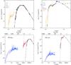 |
Fig. A.1 Fitting stellar parameters, and compilation of the stellar irradiation for two examples, TW Hya (left) and AB Aur (right). The upper plots show measured photometric fluxes (coloured symbols) as function of wavelength λ, in comparison to our best fitting, reddened Phoenix stellar atmosphere model spectrum (black), and the averaged observed FUV data (orange). The lower plots show the de-reddened surface intensities Iν(r = R⋆) (black), and the averaged, de-reddened FUV data (λ> 91.2 nm, red). The blue lines show fits to de-absorbed X-ray data, using a two-component X-ray gas emission model (energy E> 0.1 keV). The dashed grey line marks the EUV regime in between, which is assumed to be absorbed by neutral hydrogen between the star and the disk and hence disregarded in the disk model. The dashed magenta lines show quick parametric fits to the UV and X-ray data, see Eqs. (A.1) and (A.2) and text, not used for the TW Hya and AB Aur models. |
Appendix A.2: Stellar UV irradiation
The UV irradiation by the central star is much more difficult to determine, and hampered by the lack of high-quality UV data, especially in the hard FUV region (<130 nm), and for Lyα. We have systematically scanned and collected UV data from IUE, FUSE, HST/STIS, HST/COS, and HST/ACS. These data have been re-binned and collated, using the inverse square of the flux uncertainties as weighting factors, following the idea used by Valenti et al. (2000, 2003). The results of this data collection will be described elsewhere (Dionatos et al. 2015, in prep.).
For many objects, the UV data is poor and incomplete, and we have to use template stars or other tools to complete it. One option is to use a simple powerlaw Iλ ∝ λpUV, or 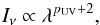 (A.1)where the proportionality constant and the UV powerlaw index pUV can be roughly fitted to the existing data, or in order to fill in gaps in the data. For TW Hya and AB Aur, however, the UV data quality is excellent, and we can directly use the data to determine the UV irradiation, see Fig. A.1 and Table A.1.
In case of the Herbig Ae/Be stars, the UV data seems mostly photospheric in character, still having absorption lines down to wavelengths of about 150 nm and below, but at even shorter wavelengths, the spectrum changes character, is dominated by emission lines and is in excess to photospheric models. The soft part of the UV data can then be used to improve the fits of the stellar parameters and AV. For AB Aur, we do not need to pick T⋆ from the literature. We find good agreement between the UV data and our photospheric model with T⋆ = 9550 K down to about 130 nm, in excellent agreement with (DeWarf et al. 2003).
Assumed/derived stellar parameters for two example objects.
Appendix A.3: Stellar X-ray irradiation
X-ray data were obtained by using archival and new data from the two X-ray observatories XMM-Newton (Jansen et al. 2001) and Chandra (Weisskopf et al. 2000). The spectra were extracted using the software of either science centres (SAS and CIAO). To get the source spectra, we select a circular extraction region around the center of the emission, while the background area contained a large source-free area on the same CCD. The extraction tools (EVSELECT for XMM and SPECEXTRACT for Chandra) delivered the source and background spectra as well as the redistribution matrix and the ancilliary response files.
The extracted spectra were then fitted with the X-ray emission model XSPEC (Arnaud 1996) assuming a collisionally ionised plasma (VAPEC) and a model for an absorption column (WABS). The element abundance values in the VAPEC models were set to typical values for pre-main sequence stars, as chosen by the XEST project (Güdel et al. 2007). Either a one component (1T), a two component (2T) or a three component (3T) emission model is fitted to the data. Highly absorbed sources or scarce data allow only for 1T fits. The fit delivers an absorption column density towards the source NH, and a plasma emission temperature TX and an emission measure EM for each component. Finally, the unabsorbed spectrum is calculated after setting the absorption column density parameter to zero, and the flux is derived by integrating over the energy range 0.3−10 keV.
In cases where no detailed X-ray data are available, a more simple two-parameter approach is used considering a free-free (bremsstrahlung) continuum with total luminosity LX and a fitted X-ray emission temperature TX,fit as 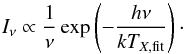 (A.2)Table A.1 shows that TX,fit results to be close to the highest X-ray component temperatures found, whereas the mean temperature ⟨ TX ⟩ (linear mean of component temperatures, weighted by component emission masses) would result in a very bad fit and should not be used in Eq. (A.2). The unabsorbed X-ray emission spectrum is finally converted to units of surface intensities Iν(r = R⋆) [erg/cm2/ s/Hz/sr], using the previously determined values for d and R⋆, and merged with the UV data and photospheric model spectrum.
Appendix A.4: Background radiation
Protoplanetary disks are irradiated not only by the central star, but also from the environment. We assume an isotropic interstellar (IS) background radiation field  with 3 components, the IS UV-field (created by distant O-stars), the cosmic background (CMB, approximated by a 2.7 K Planckian), and an infrared background radiation field
  (created by distant stars and molecular clouds).
 |
Fig. A.2 Results for the T Tauri reference model with artificially large PAH abundance (fPAH = 10), showing independent results from ProDiMo, MCMax and MCFOST with PAHs in radiative equilibrium. The upper left figure shows the well-mixed dust and neutral PAH opacities. ProDiMo opacities are shown by lines, separately for dust (black = extinction, red = absorption, blue = scattering) and PAHs (green, only absorption), MCMax and MCFOST opacities are shown by dots (combined dust+PAH opacities). The upper right figure shows the computed SEDs with a zoom-in on the prominent PAH emission features at 3.3 μm, 6.2 μm, 7.6 μm, 8.6 μm, 11.3 μm and 13.5 μm. The lower left plot shows the assumed gas densities ρgas (black) and derived (settled) dust densities ρdust (red) for a series of vertical cuts at radius r as labelled. The PAH densities are given by ρPAH ≈ 0.00132 × ρgas for fPAH = 10. The lower middle and lower right plots compare the computed dust and PAH temperatures betweenMCMax (green), MCFOST (blue), and ProDiMo (black). |
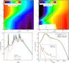 |
Fig. A.3 Comparison of PAH results between full treatment with stochastic quantum heating, and simplified method assuming the PAHs to be in radiative equilibrium. The reference model with artificially increased PAH abundance fPAH = 10 is considered. The upper left plot shows the mean PAH temperature ⟨ TPAH ⟩, and the upper right plot shows the relative width of the PAH temperature distribution function σT/ ⟨ TPAH ⟩ where |
The interstellar UV field is approximated by a 20000 K-black-body with a tiny dilution factor Wdil = 9.85357 × 10⁻¹⁷ such that χISM = 1 corresponds to the integrated standard IS UV field of Draine & Bertoldi (1996) (A.3)For the infrared background field , we take the spectral shape from (Mathis et al. 1983, their Tables A.3 and B.1), and adjust the parameter
  such that the integrated background intensity equals
  (A.4)A blackbody would accomodate its temperature to Tback is this background radiation field. Tback limits the dust temperatures in the disk, because when including the star as additional light source, the temperatures can only increase. Without the infrared contribution
  the background temperature results to be 2.97 K, but we can increase to simulate a disk in close proximity to, e.g., a star formation region which provides additional IR background radiation, with expected impact on the mm-slope (see Sect. 5.3.3). For example, to achieve Tback = 5 K and 10 K, values for
  and 92 are required, respectively. The original work of Mathis et al. (1983, i.e.
  is derived from stars and molecular clouds at a distance at 10 kpc from the Galactic centre.
When calculating spectral fluxes from a model with background radiation, we need to subtract the background as  (A.5)The background subtraction (Eq. (A.5)) is important in particular at long wavelengths where the CMB is bright. For example, at λ = 1 cm, the CMB multiplied by solid angle
  is 15 × stronger than the disk signal from the reference model. Equation (A.5) is also necessary to make the results independent of considered image size (as long as the disk is well contained in the image). We note, however, that Eq. (A.5) can lead to negative fluxes, for example an edge-on disk in the UV or whenever the disk appears darker than the background at the considered wavelength, for example the “silhouette disks” in the Orion nebula.
Appendix B: The PAH temperature distribution
Figure A.2 shows some results for the T Tauri reference model introduced in Sect. 5, but, in order to demonstrate the effects, with an artificially large PAH abundance of fPAH = 10. The dust in the outer disk parts is strongly concentrated towards the midplane, whereas the PAH molecules stay co-spatial with the gas by assumption. In all optically thin regions, and in the surface of the inner rim, the PAH temperatures are higher by a large factor ~ 1.5−2 as compared to the dust temperatures, simply due to the very blue absorption characteristic of the PAHs which facilitates radiative heating. In contrast, in the optically thick midplane of the disk, we find TPAH ≈ Tdust as expected. The PAH emission features result from the large temperature contrast between PAHs and dust in the optically thin upper and inner disk regions <(1−10) AU, depending on wavelength, see Fig. A.3. In the outer optically thin disk regions, the PAH temperature re-increases due to the interstellar UV irradiation.
The detailed physical modelling of the PAH molecules with the Monte Carlo codes allows for a treatment of the quantum heating by single photons absorption events by the PAHs, followed by radiative cooling, which leads to a stochastic PAH temperature distribution p(T) at every point in the model. In the following, we can thereby check the validity of our simplified treatment of the PAHs in radiative equilibrium, as outlined in Sect. 3.8. The PAH emissivity [erg/s/Hz/sr /PAH-molecule] is given by 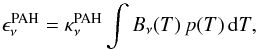 (B.1)where
  PAH-molecule] is the PAH absorption cross section and Bν(T) is the Planck function. The temperature distribution function p(T) is normalised to ∫p(T) dT = 1.
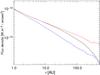 |
Fig. B.1 Comparison of radial intensity profiles in the 11.3 μm PAH emission feature obtained from the reference T Tauri model. The blue lines shows the intensity profile if dust and PAHs are assumed to have a common radiative equilibrium temperature. The black line shows the simplified treatment with independent dust and PAH temperatures, both in radiative equilibrium. The red line shows the results obtained with the full PAH treatment with a stochastic PAH temperature distribution. |
In order to quantify the mean PAH temperature and the width of the PAH temperature distribution, we consider 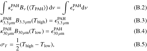 i.e. we define a high temperature to match the 3.3 μm PAH emission and a low temperature to match the continuous 30 μ PAH emission. The mean temperature ⟨ TPAH ⟩ is related to the total frequency integrated PAH emission. Usually, we find Tlow> ⟨ TPAH ⟩ >Thigh in the models, see an example in Fig. A.3, lower left part. In the example shown, the relative width of the PAH temperature distribution function is σT/ ⟨ TPAH ⟩ ≈ 15%.
Figure A.3 shows that σT/ ⟨ TPAH ⟩ anti-correlates with ⟨ TPAH ⟩. Large average PAH temperatures imply a sharply peaked temperature distribution function. The upper right plot shows which spatial disk regions are responsible for the various PAH emission features. The PAH 3.3 μm feature originates in the innermost 1 AU disk regions, whereas the 11.3 μm emission region stretches out to about 10 AU. In all cases, the PAH emissions come from borderline optically thin altitudes where the dust is not yet optically thick, and where ⟨ TPAH ⟩ ≫ Tdust. All these warm regions are characterised by quite a sharply peaked temperature distribution function σT/ ⟨ TPAH ⟩ ≈ 0.2%−30%, which explains why the fast approximate method, assuming the PAHs to be in radiative equilibrium, works so well for the SED modelling.
Figure B.1 shows, however, that there are substantial differences at larger radii, which are not important for the integral emission of the PAH features. The blue model in Fig. B.1 (assuming equal dust and PAH temperatures) fails completely to predict the PAH emission features in the SED. The black model (PAHs in radiative equilibrium) is good for the SED and sufficient to predict the intensity profiles up to ~20 AU, but only the full stochastic treatment of the PAHs (red model) can predict the intensity profile beyond ~20 AU.
Appendix C: Time-dependent chemistry
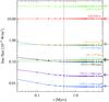 |
Fig. C.1 Computed line fluxes as function of disk age for the T Tauri reference model with time-dependent disk chemistry. Each vertical column of dots represents one disk model. The arrows on the r.h.s. indicate the results from the time-independent reference model. The vertical dashed line marks t = 0.5 Myr, after which the line fluxes do not change significantly any more. |
To investigate the effects of chemical evolution in the disk on the observable gas emission lines, we have computed additional models where the disk structure, the dust size distribution, dust settling and opacities, the dust and gas temperatures, and the internal radiation field are taken over from the reference model, but at each grid point, the chemical rate network is advanced in time from zero to 5 Myr, starting from initial concentrations typical for the dark cores of molecular clouds, see (Helling et al. 2014) for details.
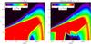 |
Fig. C.2 The CO concentration ϵ(CO) = nCO/n⟨ H ⟩ after 1 Myr (l.h.s.) compared to the CO concentration in the time-independent reference model. |
Figure C.1 shows the resulting line fluxes as function of disk age. After an initial relaxation phase which lasts a few 105 yrs, the gas emission line fluxes become constant in the model, and do not change significantly afterwards. This behaviour is a consequence of the relatively short chemical relaxation timescales in most line forming regions situated well above the icy midplane, compare Fig. 12. The chemical relaxation timescale τchem(r,z) is introduced and discussed in (Woitke et al. 2009, see Sect. 8.3 and Fig. 13 therein). The relaxation of the optical and IR lines is indeed very quick; we measure mean values of the chemical relaxation timescale as 1.2 yrs, 90 yrs, 120 yrs, 4000 yrs and 8000 yrs in the line forming regions of [OI] 6300 Å, o-H2 17 μm, CO J = 18−17, CO J = 10−9 and [OI] 63 μm, respectively.
However, the CO mm-line fluxes do not fully converge to the results obtained by the time-independent reference model, see arrows on the r.h.s. of Fig. C.1, even for integration times as long as 10 Myr. This is consistent with the very long chemical relaxation timescales ⟨ τchem ⟩ we find for those lines, namely 20 Myr, 50 Myr and 100 Myr in the line forming regions of CO J = 2−1, 13CO J = 2−1, and C18O J = 2−1, respectively.
The difference of the CO concentration between the t = 1 Myr disk model and the time-independent reference model is shown in Fig. C.2. All upper disk regions have practically indistinguishable CO concentrations, however, in the dark icy midplane (vertical visual extinction AV> 10), CO cannot freeze out directly where the dust temperature exceeds about 20 K (at radii ≲30 AU in this model). Instead, the CO is very slowly dissociated in these regions by reactions with He+ created by cosmic rays. Most of the liberated oxygen atoms re-form CO, but a small part can form other molecules with higher adsorptions energies like water, and these will freeze out immediately. This mechanism provides a slowly ticking chemical clock in the dark midplane regions of protoplanetary disks, leading to gaseous carbon-to-oxygen ratios C/O ≈ 1 on Myr timescales between the water and the CO ice-lines, and to C/O ≫ 1 on even longer timescales, see (Öberg et al. 2011; Helling et al. 2014).
The (sub-)mm CO isotopologue line fluxes are somewhat affected by these differences, for example remainders of cold gaseous CO in the dark icy midplane can partly re-absorb the CO line photons emitted by the warm surface of the disk on the opposite side which cross the midplane. In this way, the CO isotopologue line fluxes of the time-independent model can be up to 30% larger than those of the time-dependent models. However, these effects are small compared to the impact of disk mass, size and shape, dust size distribution and settling, and the dust/gas ratio, and negligible for most optical and near-IR to far-IR lines.
We conclude that the emission lines of chemically robust gas tracers, such as CO, H2 and the oxygen atom, are little affected by time-dependent chemical effects in our models. Disk evolution will rather have an impact on those lines via the changing stellar parameters, the changing shape of the disk, and physical gas and dust evolution. See e.g. Akimkin et al. (2013) for time-dependent disk models which include those effects.
Appendix D: Properties derived from the model
The mean gas temperature in the disk ⟨ Tgas ⟩, the mean dust temperature ⟨ Tdust ⟩, the near-IR excess, the 10 μm SED amplitude, the dust absorption mm and cm-slopes βabs, and the millimetre and centimetre flux-slopes αSED, are calculated as  where ρgas is the gas mass density, ρdust = ρgas·δ the dust mass density, δ the local dust-to-gas mass ratio, dV = 2πr dr dz the volume element, d the distance,
  the spectral flux per wavelength interval,
  the flux from the naked star and the dust absorption opacity [cm2/ g(dust)].
Appendix E: Fluxes of optically thick emission lines
It is noteworthy that all observable emission lines discussed in this paper are optically thick in the reference model, with the only exception being C18O J = 2 → 1 which is borderline optically thin. For large optical depths we can use the Eddington-Barbier approximation ![\appendix \setcounter{section}{5} \begin{equation} I_\nu \approx S_{\nu}\,(\tau_\nu=1) \approx\left\{\begin{array}{ll} S_{\nu}^{\rm cont}\,(\tau_\nu^{\rm cont}=1) & \mbox{,\ \ if }|\nu-\nu_0|\gg\Delta\nu\\[0.6ex] S_{\nu}^{\rm line}\,(\tau_\nu^{\rm line}=1) & \mbox{,\ \ if }|\nu-\nu_0|\leq \Delta\nu, \end{array}\right. \label{eq:Inu} \end{equation}](/articles/aa/full_html/2016/02/aa26538-15/aa26538-15-eq490.png) (E.1)where Sν is the general source function,
(E.1)where Sν is the general source function,  the continuum source function and
  the line source function.
  and
and  are the continuum and line centre optical depth, ν0 and Δν = FWHM/ 2 are the line centre frequency and observed frequency width, respectively. If the continuum is optically thin
  , its contribution can be neglected in Eq. (E.1).
Integration over solid angle and frequency, and continuum subtraction, results in the line flux ![\appendix \setcounter{section}{5} \begin{eqnarray} F_{\rm line} &=&\int\int \left(I_\nu-I_\nu^{\rm cont}\right)\,{\rm d}\nu\,{\rm d}\Omega~~~~~~~~~~~~~~~~~~~~~~~~~~~~~~~~~~~~~~~~~~~~~~~~~~~~~~~~~~~~~~~~~~~~~~~~~~~~~~~ \nonumber\\ &\approx& 2\Delta\Omega\,\Delta\nu \left(S_{\nu}^{\rm line}(\tau_{\rm line}=1) -S_{\nu}^{\rm cont}\left(\tau_{\rm cont}=1\right)\right) \label{eq:Fline}\\ &\approx& 2\Delta\Omega\,\Delta\nu \left(B_\nu\left[T_{\rm gas}\left(\tau_{\rm line}\!=\!1\right)\right] \! -\!B_\nu\left[T_{\rm dust}\left(\tau_{\rm cont}\!=\!1\right)\right]\right) , \label{eq:Flapprox} \end{eqnarray}](/articles/aa/full_html/2016/02/aa26538-15/aa26538-15-eq499.png) where ΔΩ is the solid angle occupied by the part of the disk that is optically thick in the line, and 2Δν = FWHM is the observed frequency full width half maximum. The first approximation (Eq. (E.2)) is valid only if the excitation conditions (, ) are about constant in the line forming region, otherwise the integration over the solid angle cannot be carried out this way. The second approximation (Eq. (E.3)) is valid for LTE only. Figure 20 shows the typical situation encountered in disks where we look through a warm gas toward the cold, optically thick midplane.
where ΔΩ is the solid angle occupied by the part of the disk that is optically thick in the line, and 2Δν = FWHM is the observed frequency full width half maximum. The first approximation (Eq. (E.2)) is valid only if the excitation conditions (, ) are about constant in the line forming region, otherwise the integration over the solid angle cannot be carried out this way. The second approximation (Eq. (E.3)) is valid for LTE only. Figure 20 shows the typical situation encountered in disks where we look through a warm gas toward the cold, optically thick midplane.
Appendix F: Numerical convergence
Figure F.1 shows three series of ProDiMo models with increasing spatial resolution in the underlying numerical grid. The resulting continuum predictions like near-IR excess, 10 μm amplitude, millimetre and centimetre slopes etc. (see Sect. D) are robust. Even quick 30 × 30 models are sufficient to predict the SED and derived quantities, with an accuracy better than 5% with respect to the results from the big 160 × 150 reference model.
The grid resolution is more critical, however, when studying emission lines. A too coarse spatial grid usually leads to an over-prediction of the emission line fluxes. Most critical are lines which originate in a small portion of the disk volume, like the weak o-H2 and high-J CO lines, but also [OI] 63.2 μm and [OI] 6300 Å. Here, the radial grid resolution is more important than the vertical grid resolution. The only counter-example to this rule are the ro-vibrational CO lines which are mostly emitted directly from the surface of the inner rim in this model. Here, the vertical grid resolution is more important. In summary, we need a grid resolution of about 100 × 100 to achieve an accuracy better than 10% for all predictions, see grey shaded box in Fig. F.1.
Figure F.2 shows the numerical convergence of MC→ProDiMo chain models, when varying the spatial grid resolution in the Monte-Carlo (MC) programs. It is reassuring to see that the MC→ProDiMo chain models actually produce results that are very similar as compared to the pure ProDiMo models. For sufficient spatial resolution in the MC models (again about 100 × 100 grid points), the deviations in continuum results are smaller than 10%, and line results agree better than 15%, where most critical are the faint mid-far IR o-H2 and high-J CO lines. Other, e.g. (sub-)mm line results are more robust. There is also no obvious asymmetry in Fig. F.2, e.g. some lines are weaker whereas others are stronger when using the MC→ProDiMo chain models.
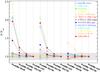 |
Fig. F.1 Various results of pure-ProDiMo models as function of spatial grid resolution. All results F are plotted with respect to the results of the reference model Fref, which has 160 × 150 radial and vertical grid points, respectively. The quantities annotated with spectral lines are emission line fluxes. |
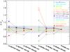 |
Fig. F.2 Various results of MC→ProDiMo chain models as function of the spatial grid resolution in the Monte-Carlo (MC) programs MCFOST and MCMax. The continuum results are directly computed from the MC model output files. The line results are obtained by passing the MC model results (densities, opacities, Tdust, radiation field, etc.) to a high-resolution (160 × 150) ProDiMo model. For further explanations, see caption of Fig. F.1. |
For sufficient spatial resolution in the MC models, the MCFOST and MCMax results show a similar pattern with respect to the pure ProDiMo reference results, i.e. the deviations between MCFOST→ProDiMo and MCMax→ProDiMo models are actually smaller than the deviations between those models and pure ProDiMo models.
Appendix G: Impacts of additional model parameters
Figure G.1 shows the impact of various model parameters on the mean CO fundamental line emission strengths and profiles. The results are discussed in Sect. 5.3.7.
Figure G.2 compares the results obtained from a model using anisotropic scattering to the reference model. The largest difference concerns the amplitude of the 10 μm silicate emission feature, the anisotropic model has a stronger amplitude by about 14%, making the feature clearly more visible in the SED plot as compared to the reference model.
Concerning the gas emission lines, we see only little effects, and no clear trend. The disk is mostly UV illuminated from the top, which requires at least one scattering event in the borderline optically thin disk surface layers. Since an
angle-dependent treatment of dust scattering favours forward scattering, one would expect the UV illumination of the disk from above to be reduced, because ≈90° scattering events seem to be required. However, this does not seem to be entirely true. The question whether a scattered UV photon reaches the disk or not is simply determined by whether the photon is scattered upwards or downwards, which is a 50%/50% chance even for anisotropic scattering. With anisotropic scattering, we rather redistribute the entry points where the scattered photons enter the disk, favouring the outer disk regions, and their initial entry angle. Multiple scattering also reduces the effects.
We measure line flux and FWHM differences of order 10%, with no clear trend, the only exception being CO J = 10 → 9 with is actually enhanced by 28%. These results are close to the “noise level” expected from various numerical effects in the models, compare Figs. F.1 and F.2.
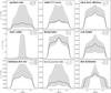 |
Fig. G.1 Effects of selected stellar, gas, dust and disk shape parameters on CO fundamental emission line profiles. Each part figure shows mean line profiles averaged over all computed CO υ = 1 → 0R-branch and P-branch emission lines, continuum subtracted and convolved with a 12 km s-1 Gaussian (resolution R ≈ 25 000). The thick full lines show the reference model, identical in every part figure. The shaded areas indicate the changes caused by single parameter variations, where the dashed and dotted lines correspond to the changed parameter values as annotated. Non-depicted parameters have less influence on the CO fundamental emission, for example the X-ray luminosity LX, compare Fig. 18. |
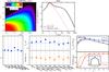 |
Fig. G.2 Comparison of results between models using isotropic and anisotropic scattering. Both models are MCMax→ProDiMo chain models. The results from the anisotropic model are shown with respect to the results obtained from the isotropic (reference) model. Depicted quantities are explained in Fig 4. The visibility plot is omitted here. |
All Tables
Assumptions about disk shape, grain size, opacities, dust settling and PAHs in different thermo-chemical disk models.
Unsettled dust properties in the reference model in comparison to a MRN size distribution and uniform a = 0.1 μm dust particles.
Negative logarithmic derivative of the Planck function, −∂log Bν(T) /∂log λ, as function of temperature and wavelength.
All Figures
|
Fig. 1 Three figures visualising our disk modelling approach concerning disk shape and dust settling. This particular model has two radial zones, with a (dust and gas-free) gap between r = 1 AU to r = 5 AU. The outer zone is featured by a tapered outer edge. The left plot shows the hydrogen nuclei particle density n⟨ H ⟩(r,z). The middle and right plots show the local gas/dust ratio, and the mean dust particle size, respectively. These two properties are not constant throughout the disk, but depend on r and z through dust settling, see Sect. 3.5. From top to bottom, the two red dashed contour lines show the radial optical depth, in terms of the visual extinction, AV,rad = 0.01 and AV,rad = 1, and the two dashed black contours show the vertical optical depths AV = 1 and AV = 10. In the middle and r.h.s. plots, the vertical AV = 10 contour line has been omitted. |
| In the text | |
|
Fig. 2 Dust opacities used for the standard disk radiative transfer modelling, with parameters amin = 0.05 μm, amax = 3 mm, apow = 3.5, and 15% amorphous carbon by volume. The extinction per dust mass is shown in black, absorption in red, and scattering in blue. Results shown with lines for ProDiMo, open symbols for MCMax, and full symbols for MCFOST – all of which agree. The red star represents the value of 3.5 cm2/ g(dust) at 850 μm used by Andrews & Williams (2005) to determine disk masses from sub-mm fluxes. |
| In the text | |
|
Fig. 3 Dust absorption coefficient per dust mass as function of dust size and material parameters. The black line is identical in every part plot, with parameter values as used in the reference model, our dust standard opacities, see Table 3. The upper two figures show the dependencies on minimum and maximum particle size, amin and amax. The lower two plots show the dependencies on dust size powerlaw index apow and on the volume fraction of amorphous carbon. 25% porosity and maximum hollow volume ratio |
| In the text | |
|
Fig. 4 Summary of results from the reference model. Top row: assumed gas density structure n⟨ H ⟩(r,z) with overplotted radial (red) and vertical (black) optical depths AV = 1 dashed contours, computed SED, and visibilities. In the visibility plot, the coloured areas show V2 for all baseline orientations at 3 different wavelengths, with a zoom-in on the first 30 m. Lower row: other resulting quantities. The left plot shows the mean dust and gas temperatures (in units of 10 K), the near-IR excess (in units of 0.05 L⊙) and the logarithmic SED slopes at mm and cm wavelengths. The centre plot shows calculated line fluxes and full widths at half maximum (FWHM). The right plot shows some results for the CO fundamental ro-vibrational line emissions, line fluxes as function of rotational quantum number J for the R-branch and the P-branch, as well as computed FWHM for those lines. The inserted figure shows the line profile averaged over all emission lines, scaled from 0 (continuum) to 1 (maximum). |
| In the text | |
|
Fig. 5 Results from the T Tauri reference model, but assuming uniform 0.1 μm sized dust particles and astronomical silicate Mie opacities. Depicted quantities are shown with respect to the reference model, and explained in the caption of Fig. 4. |
| In the text | |
|
Fig. 6 Two variants of (1 + 1)D hydrostatic disk models. Depicted quantities are explained in Fig. 4, but shown here in comparison to the reference model. The upper half shows the results for the simplified hydrostatic model based on the dust temperature Tdust and a constant molecular weight, i.e. sound speed |
| In the text | |
|
Fig. 7 Effects of disk flaring and dust settling on all observables, with respect to the reference model. The upper set of figures shows a model with less flaring as compared to the reference model β = 1.05, and the lower half shows a model with stronger dust settling αsettle = 10-4. See Fig. 6 for further explanations. |
| In the text | |
|
Fig. 8 Effect of dust and disk parameters on model SED at distance 140 pc and inclination 45°. The thick full black line is the reference model (identical in every part figure), whereas the green shaded area indicates the effect of a single parameter on the SED, where the dashed and dotted lines correspond to the changed parameter values as annotated. Top row: dust mass Mdust, scale height H0, and flaring exponent β. Second row: inner radius Rin, column density powerlaw index ϵ, and dust settling parameter αsettle. Third row: maximum grain size amax, dust size powerlaw index apow, and volume ratio of amorphous carbon. The dependencies of the SED on the tapering-off radius Rtap (not shown), on the outer radius Rout (not shown), and on the minimum dust particle size amin (not shown) are less than the one shown for ϵ. |
| In the text | |
|
Fig. 9 Effects of selected dust and disk shape parameters on continuum visibilities at 1.6 μm (blue), 10 μm (green) and 1.3 mm (red). Distance is 140 pc. The squared visibility V2 (fraction of correlated flux) is shown as function of baseline [cm] /1000 /λ [cm] for baseline orientation along the major axis of the disk on the sky. The abscissa on top is the corresponding maximum observable spatial scale [cm] = 0.6·d [cm] /baseline [kλ] /1000. The full lines show the reference model, identical in every part figure. The dashed and dotted lines correspond to the changed parameter values as annotated. Non-depicted parameters have less influence on the visibilities, for example amax. See Table 3 for explanations of parameter symbols. |
| In the text | |
|
Fig. 10 Impact of model parameters on the millimetre SED slope (left) and centimetre SED slope (right), as defined by Eqs. (D.7) and (D.8), respectively. The model parameters which have been varied are listed to the right of each plot (see Table 3 for explanations of the symbols), along with the ranges explored. The colours indicate different groups of model parameters. Gas and dust masses are shown in black, disk shape parameters in green, and dust size, material and settling parameters in orange. The changes of the observable quantity, here e.g. the mm-slope, caused by varying a particular model parameter, are shown with arrows. The original value of the observable quantity is shown by the red point marked with “reference model” (for example, 2.4 for the mm-slope), where the top x-axis provides an absolute scale, and the bottom x-axis provides a relative scale with respect to the value obtained by the reference model. The arrows indicate the direction and magnitude of changes caused. Leftward arrows indicate a flattening of the SED, rightward arrows a steepening. The corresponding parameter values are shown to the left and right of the “–” to the right of each plot. For example, increasing the disk mass Mdisk from the reference value to 0.1 M⊙ results in a flatter SED |
| In the text | |
|
Fig. 11 Correlation between computed SED mm-slope (as measured between 850 μm and 1.3 mm) and midplane dust temperature at r = 50 AU for models with identical dust properties and disk mass. Varied parameters include gas/dust (at constant Mdust), Rin, Rtap, ϵ, γ, H(100 AU), β and αsettle, i.e. the green disk shape parameters in Fig. 10 and dust settling. |
| In the text | |
|
Fig. 12 Line emitting regions in the reference model. The surrounded areas are responsible for 50% of the vertically emitted line fluxes as annotated. The black dashed contours show the hydrogen nuclei particle density log n⟨ H ⟩(r,z). The yellow dotted contour line shows the upper boundary of the molecular layer where nCO/n⟨ H ⟩ = 10-5. |
| In the text | |
|
Fig. 13 “Impactogram” of the [OI] 63.2 μm emission line. The absolute line flux is depicted on the top abscissa, as well as relative to the reference model at the bottom. Leftward arrows indicate a weakening of the line, and rightward arrows a strengthening of the line, due to changes of single model parameter as indicated on the r.h.s. The colours indicate groups of parameters. Gas and dust masses are shown in black, heating parameters in blue, disk shape parameters in green, and dust parameters in orange. See Fig. 10 for further explanations. |
| In the text | |
|
Fig. 14 Impact of model parameters on the CO J = 18 → 17 emission line at 144.87 μm, see Fig. 10 for explanations. |
| In the text | |
|
Fig. 15 Predicted behaviour of the 12CO, 13CO and C18O J = 2 → 1 isotopologue lines around 1.3 mm. The left plot shows the impact of model parameters on the predicted 12CO line flux, see Fig. 10 for more explanations. The two figures on the right show the impacts of model parameters on the 12CO /13CO and 13CO/C18O line ratios. Note that the direction of effects is sometimes inversed on the r.h.s., for example the dependency on disk flaring parameter β. Less flaring leeds to weaker CO lines in general, but to larger line ratios. On the right, both an increase and a decrease of the amorphous carbon dust volume fraction Vol(AC) lead to higher line ratios, here the larger arrows correspond to Vol(AC) = 0%. |
| In the text | |
|
Fig. 16 Understanding (sub-)mm CO isotopologue line ratios. The 13CO line is weaker, because it approaches τline = 1 at smaller radii. Similar apparent radii (and fluxes) of the 12CO and 13CO lines can be obtained by making the outer disk edge sharp. |
| In the text | |
|
Fig. 17 CO υ = 1 → 0 line velocity profiles predicted by the reference model, continuum subtracted and convolved with a 12 km s-1 Gaussian (resolution R ≈ 25 000). The R(10) and R(35) lines plotted in red are selected for further study of the model parameters impacts in Fig. 18. |
| In the text | |
|
Fig. 18 Impact of model parameters on ro-vibrational CO emission. On the l.h.s, the υ = 1 → 0R(10) line has been selected to study the effects of changing model parameters on line flux. The r.h.s. shows the R(35) /R(10) line ratio, a measure for the “CO rotational excitation temperature”. Large line ratios indicate emission from hot CO. Note that the direction of parameter impact is often reversed on the r.h.s., i.e. weak lines are usually emitted from a tiny area of hot gas, whereas strong lines are emitted from an extended area of cool gas. See Fig. 10 for further explanations. |
| In the text | |
|
Fig. 19 Impact of inner disk radius Rin on CO υ = 1 → 0 line emission fluxes and FWHM. The black line shows the computed R(10) line fluxes for the reference model, when varying Rin between 0.07 AU and 100 AU. The blue line shows the R(10) /R(35) line ratio, and the red line shows the computed R(10) line widths. |
| In the text | |
|
Fig. 20 Understanding optically thick CO ro-vibrational emission lines. The sketch can either represent the inner rim horizontally, or a distant disk column vertically. The gas and dust temperature structure is connected to τUV, the dust optical depth in the UV. High-J and low-J CO emission lines have different line optical depths, so their fluxes probe the contrast between gas and dust temperatures at different depths. |
| In the text | |
|
Fig. A.1 Fitting stellar parameters, and compilation of the stellar irradiation for two examples, TW Hya (left) and AB Aur (right). The upper plots show measured photometric fluxes (coloured symbols) as function of wavelength λ, in comparison to our best fitting, reddened Phoenix stellar atmosphere model spectrum (black), and the averaged observed FUV data (orange). The lower plots show the de-reddened surface intensities Iν(r = R⋆) (black), and the averaged, de-reddened FUV data (λ> 91.2 nm, red). The blue lines show fits to de-absorbed X-ray data, using a two-component X-ray gas emission model (energy E> 0.1 keV). The dashed grey line marks the EUV regime in between, which is assumed to be absorbed by neutral hydrogen between the star and the disk and hence disregarded in the disk model. The dashed magenta lines show quick parametric fits to the UV and X-ray data, see Eqs. (A.1) and (A.2) and text, not used for the TW Hya and AB Aur models. |
| In the text | |
|
Fig. A.2 Results for the T Tauri reference model with artificially large PAH abundance (fPAH = 10), showing independent results from ProDiMo, MCMax and MCFOST with PAHs in radiative equilibrium. The upper left figure shows the well-mixed dust and neutral PAH opacities. ProDiMo opacities are shown by lines, separately for dust (black = extinction, red = absorption, blue = scattering) and PAHs (green, only absorption), MCMax and MCFOST opacities are shown by dots (combined dust+PAH opacities). The upper right figure shows the computed SEDs with a zoom-in on the prominent PAH emission features at 3.3 μm, 6.2 μm, 7.6 μm, 8.6 μm, 11.3 μm and 13.5 μm. The lower left plot shows the assumed gas densities ρgas (black) and derived (settled) dust densities ρdust (red) for a series of vertical cuts at radius r as labelled. The PAH densities are given by ρPAH ≈ 0.00132 × ρgas for fPAH = 10. The lower middle and lower right plots compare the computed dust and PAH temperatures betweenMCMax (green), MCFOST (blue), and ProDiMo (black). |
| In the text | |
|
Fig. A.3 Comparison of PAH results between full treatment with stochastic quantum heating, and simplified method assuming the PAHs to be in radiative equilibrium. The reference model with artificially increased PAH abundance fPAH = 10 is considered. The upper left plot shows the mean PAH temperature ⟨ TPAH ⟩, and the upper right plot shows the relative width of the PAH temperature distribution function σT/ ⟨ TPAH ⟩ where |
| In the text | |
|
Fig. B.1 Comparison of radial intensity profiles in the 11.3 μm PAH emission feature obtained from the reference T Tauri model. The blue lines shows the intensity profile if dust and PAHs are assumed to have a common radiative equilibrium temperature. The black line shows the simplified treatment with independent dust and PAH temperatures, both in radiative equilibrium. The red line shows the results obtained with the full PAH treatment with a stochastic PAH temperature distribution. |
| In the text | |
|
Fig. C.1 Computed line fluxes as function of disk age for the T Tauri reference model with time-dependent disk chemistry. Each vertical column of dots represents one disk model. The arrows on the r.h.s. indicate the results from the time-independent reference model. The vertical dashed line marks t = 0.5 Myr, after which the line fluxes do not change significantly any more. |
| In the text | |
|
Fig. C.2 The CO concentration ϵ(CO) = nCO/n⟨ H ⟩ after 1 Myr (l.h.s.) compared to the CO concentration in the time-independent reference model. |
| In the text | |
|
Fig. F.1 Various results of pure-ProDiMo models as function of spatial grid resolution. All results F are plotted with respect to the results of the reference model Fref, which has 160 × 150 radial and vertical grid points, respectively. The quantities annotated with spectral lines are emission line fluxes. |
| In the text | |
|
Fig. F.2 Various results of MC→ProDiMo chain models as function of the spatial grid resolution in the Monte-Carlo (MC) programs MCFOST and MCMax. The continuum results are directly computed from the MC model output files. The line results are obtained by passing the MC model results (densities, opacities, Tdust, radiation field, etc.) to a high-resolution (160 × 150) ProDiMo model. For further explanations, see caption of Fig. F.1. |
| In the text | |
|
Fig. G.1 Effects of selected stellar, gas, dust and disk shape parameters on CO fundamental emission line profiles. Each part figure shows mean line profiles averaged over all computed CO υ = 1 → 0R-branch and P-branch emission lines, continuum subtracted and convolved with a 12 km s-1 Gaussian (resolution R ≈ 25 000). The thick full lines show the reference model, identical in every part figure. The shaded areas indicate the changes caused by single parameter variations, where the dashed and dotted lines correspond to the changed parameter values as annotated. Non-depicted parameters have less influence on the CO fundamental emission, for example the X-ray luminosity LX, compare Fig. 18. |
| In the text | |
|
Fig. G.2 Comparison of results between models using isotropic and anisotropic scattering. Both models are MCMax→ProDiMo chain models. The results from the anisotropic model are shown with respect to the results obtained from the isotropic (reference) model. Depicted quantities are explained in Fig 4. The visibility plot is omitted here. |
| In the text | |
Current usage metrics show cumulative count of Article Views (full-text article views including HTML views, PDF and ePub downloads, according to the available data) and Abstracts Views on Vision4Press platform.
Data correspond to usage on the plateform after 2015. The current usage metrics is available 48-96 hours after online publication and is updated daily on week days.
Initial download of the metrics may take a while.