| Issue |
A&A
Volume 689, September 2024
|
|
|---|---|---|
| Article Number | A92 | |
| Number of page(s) | 18 | |
| Section | Interstellar and circumstellar matter | |
| DOI | https://doi.org/10.1051/0004-6361/202450865 | |
| Published online | 04 September 2024 | |
A JWST/MIRI analysis of the ice distribution and polycyclic aromatic hydrocarbon emission in the protoplanetary disk HH 48 NE
1
Leiden Observatory, Leiden University,
PO Box 9513,
2300 RA
Leiden, The Netherlands
2
Institute of Astronomy, Department of Physics, National Tsing Hua University,
Hsinchu, Taiwan
3
Department of Chemistry, University of California,
Berkeley, CA
94720-1460, USA
4
Institut des Sciences Moléculaires d’Orsay, CNRS, Univ. Paris-Saclay,
91405
Orsay, France
5
Institute for Astronomy, University of Hawai’i at Manoa,
2680 Woodlawn Drive,
Honolulu, HI
96822, USA
6
Astrochemistry Laboratory, NASA Goddard Space Flight Center,
8800 Greenbelt Road,
Greenbelt, MD
20771, USA
7
Department of Physics, Catholic University of America,
Washington, DC
20064, USA
8
Physikalisch-Meteorologisches Observatorium Davos und Weltstrahlungszentrum (PMOD/WRC),
Dorfstrasse 33,
7260,
Davos Dorf, Switzerland
9
Centre for Interstellar Catalysis, Department of Physics and Astronomy, Aarhus University,
8000
Aarhus, Denmark
10
Department of Astronomy, University of Virginia,
Charlottesville, VA
22904, USA
11
Jet Propulsion Laboratory, California Institute of Technology,
4800 Oak Grove Drive,
Pasadena, CA
91109, USA
12
Department of Chemistry, Massachusetts Institute of Technology,
Cambridge, MA
02139, USA
13
National Radio Astronomy Observatory,
Charlottesville, VA
22903, USA
14
Center for Astrophysics I Harvard & Smithsonian,
60 Garden St.,
Cambridge, MA
02138, USA
15
Physique des Interactions Ioniques et Moléculaires, CNRS, Aix Marseille Univ.,
13397
Marseille, France
16
INAF – Osservatorio Astrofisico di Catania,
via Santa Sofia 78,
95123
Catania, Italy
17
Department of Physics, University of Central Florida,
Orlando, FL
32816, USA
18
Max Planck Institute for Astronomy,
Königstuhl 17,
69117
Heidelberg, Germany
19
Laboratory for Astrophysics, Leiden Observatory, Leiden University,
PO Box 9513,
2300 RA
Leiden, The Netherlands
20
Max-Planck-Institut für extraterrestrische Physik,
Giessenbachstraße 1,
85748
Garching bei München, Germany
Received:
24
May
2024
Accepted:
11
July
2024
Abstract
Context. Ice-coated dust grains provide the main reservoir of volatiles that play an important role in planet formation processes and may become incorporated into planetary atmospheres. However, due to observational challenges, the ice abundance distribution in protoplanetary disks is not well constrained. With the advent of the James Webb Space Telescope (JWST), we are in a unique position to observe these ices in the near- to mid-infrared and constrain their properties in Class II protoplanetary disks.
Aims. We present JWST Mid-InfraRed Imager (MIRI) observations of the edge-on disk HH 48 NE carried out as part of the Direc- tor’s Discretionary Early Release Science program Ice Age, completing the ice inventory of HH 48 NE by combining the MIRI data (5–28 μm) with those of NIRSpec (2.7–5 μm).
Methods. We used radiative transfer models tailored to the system, including silicates, ices, and polycyclic aromatic hydrocarbons (PAHs) to reproduce the observed spectrum of HH 48 NE with a parameterized model. The model was then used to identify ice species and constrain spatial information about the ices in the disk.
Results. The mid-infrared spectrum of HH 48 NE is relatively flat, with weak ice absorption features. We detect CO2, NH3, H2O, and tentatively CH4 and NH4+. Radiative transfer models suggest that ice absorption features are produced predominantly in the 50–100 au region of the disk. The CO2 feature at 15 μm probes a region closer to the midplane (z/r = 0.1–0.15) than the corresponding feature at 4.3 μm (z/r = 0.2–0.6), but all observations trace regions significantly above the midplane reservoirs where we expect the bulk of the ice mass to be located. Ices must reach a high scale height (z/r ~ 0.6; corresponding to a modeled dust extinction Av ~ 0.1), in order to be consistent with the observed vertical distribution of the peak ice optical depths. The weakness of the CO2 feature at 15 μm relative to the 4.3 μm feature and the red emission wing of the 4.3 μm CO2 feature are both consistent with ices being located at a high elevation in the disk. The retrieved NH3 abundance and the upper limit on the CH3OH abundance relative to H2O are significantly lower than those in the interstellar medium, but consistent with cometary observations. The contrast of the PAH emission features with the continuum is stronger than for similar face-on protoplanetary disks, which is likely a result of the edge-on system geometry. Modeling based on the relative strength of the emission features suggests that the PAH emission originates in the disk surface layer rather than the ice absorbing layer.
Conclusions. Full wavelength coverage is required to properly study the abundance distribution of ices in disks. To explain the pres- ence of ices at high disk altitudes, we propose two possible scenarios: a disk wind that entrains sufficient amounts of dust, and thus blocks part of the stellar UV radiation, or vertical mixing that cycles enough ices into the upper disk layers to balance ice photodesorption from the grains.
Key words: radiative transfer / scattering / solid state: volatile / planets and satellites: formation / protoplanetary disks / infrared: general
Corresponding author; This email address is being protected from spambots. You need JavaScript enabled to view it.
NASA Hubble Fellowship Program Sagan Fellow.
© The Authors 2024
 Open Access article, published by EDP Sciences, under the terms of the Creative Commons Attribution License (https://creativecommons.org/licenses/by/4.0), which permits unrestricted use, distribution, and reproduction in any medium, provided the original work is properly cited.
This article is published in open access under the Subscribe to Open model. This email address is being protected from spambots. You need JavaScript enabled to view it. to support open access publication.
1 Introduction
The composition of planetesimals, comets, and eventually plan- ets is determined in large part by the composition of their building blocks: ice-coated dust grains. Ices are the dominant carriers of volatiles in planet-forming regions (Pontoppidan et al. 2014; Walsh et al. 2015), and set for a large part the spatial distribution of volatiles in the disk (McClure 2019; Banzatti et al. 2020; Sturm et al. 2022; Banzatti et al. 2023). Ices not only play a crucial role in the disk chemistry, but also in planet formation processes (e.g., Öberg & Bergin 2016; Drążkowska et al. 2016). Unlike the gas present in the protoplanetary disk, ices are directly incorporated into the cores of planets, comets, and icy moons (Öberg et al. 2023b). Mapping ices in disks at different stages of their evolution is therefore important to under- stand the initial building blocks available for planet formation.
With the advent of the James Webb Space Telescope (JWST) we are in the unique position to target the ice absorption bands in the mid-infrared (2-15 μm) with sufficient angular resolution to search for spatial variations in the distribution of protoplanetary disk ices in nearby star-forming regions. In the earlier stages of the star formation sequence, when the natal cloud or envelope has high line-of-sight AV (Molecular clouds, Class 0 protostars, Class I protostars), ices have been readily observed in detail with ISO, Spitzer (Boogert et al. 2015), Akari (Aikawa et al. 2012; Noble et al. 2013), ground based observatories, and JWST (Yang et al. 2022; McClure et al. 2023; Rocha et al. 2024; Brunken et al. 2024). However, in late-stage protoplanetary disks after the envelope has dissipated (Class II systems), the contrast of these ice species with respect to the continuum from the warm inner disk is only detectable if the star and bright inner disk is blocked by the disk. This is the case for edge-on disks, which makes them ideal laboratories to study ices in Class II systems (Pontoppidan et al. 2005, 2007; Terada et al. 2007; Schegerer & Wolf 2010; Terada & Tokunaga 2012; Terada et al. 2012; Terada & Tokunaga 2017). Since these sources require high sensitivity to be observed, due to their edge-on nature, JWST is the first observatory that allows for spatially resolved, sensitive observa- tions of these systems with full wavelength coverage in the near- and mid-infrared. An initial analysis of Near-Infrared Spectrograph (NIRSpec, Jakobsen et al. 2022) data of the edge-on disk HH 48 NE detected spatially resolved ice features for the first time in a disk, including the trace species NH3, OCS, OCN−, and 13CO2, and revealed a surprisingly large vertical extent of H2O, CO2, and CO ice absorption (Sturm et al. 2023a). In this paper, we present new Mid-InfraRed Imager (MIRI, Rieke et al. 2015) observations of the same source to complete the inventory of ice features observable with JWST.
Our radiative transfer models and interpretation of JWST NIRSpec observations have shown that the complex scattering light path through edge-on disks precludes a straightforward analysis of the ice features, so that ice abundance distribu- tions can only be constrained by radiative transfer modeling of multi-wavelength observations (Sturm et al. 2023b,a). Ice fea- ture profiles become distorted by scattering (Dartois et al. 2024), and their optical depths do not depend linearly on the column density along a direct line-of-sight toward the star because the multiple light paths through the disk partially ‘dilute’ the absorp- tion profiles. Additional modeling diagnostics of the different ice absorbing regions are necessary in order to understand the spatial distribution of abundances in disks.
Another important element of protoplanetary disks are the Polycyclic Aromatic Hydrocarbons (PAHs). These big molecules (that in many aspects resemble small dust grains) play a cru- cial role in the charge balance, chemistry, and heating/cooling of the disk and could contain a significant fraction of the avail- able carbon (Tielens 2008; Kamp 2011). PAHs can be excited by UV radiation and cool efficiently through mid-infrared emission features. These features are attributed to the stretching of C–H (3.3 μm) and C–C (6.23, 7.7 μπι) bonds, in-plane (8.4 μm) and out-of-plane (11.27 μm) C–H bending motions or a combination of both (5.4, 5.65 μm). The shape and comparative strength of the features can vary depending on the excitation state, charge, size distribution and hydrogenation (Draine & Li 2007; Boersma et al. 2009; Geers et al. 2009; Maaskant et al. 2014). The distri- bution and excitation of PAHs in protoplanetary disks has been actively studied (Habart et al. 2006; Visser et al. 2007; Geers et al. 2007; Boutéraon et al. 2019; Kokoulina et al. 2021). Mod- eling shows that K–M stars (T* < 4200 K) lack UV flux to excite the PAHs (Geers et al. 2009). PAH features have been detected in numerous Herbig Ae/Be stars, but not in T Tauri systems with a spectral type later than G8 (Geers et al. 2006; Tielens 2008; Maaskant et al. 2014; Lange et al. 2023), except for the edge-on disk around Tau 042021 (Arulanantham et al. 2024). The authors suggest that the unique geometry of edge-on sys- tems, which obstructs the thermal emission from the inner disk, enables the detection of the comparatively weaker PAH emission from T Tauri stars at mid-infrared wavelengths.
The paper is organized as follows: we first describe the details of the observations in Sect. 2 and the results that can be directly inferred from the observations in Sect. 3. Then we describe the model setup for simulating observations of ices in protoplanetary disks in Sect. 4 and use these models to inter- pret the ice composition, and abundance distribution of the HH 48 NE disk in Sect. 5. Finally, we discuss the implications of our findings and the prospects of analyzing ices in edge-on protoplanetary disks in Sect. 6. We summarize our findings in Sect. 7.
2 Description of observations
We present new observations of the HH 48 system using MIRI/MRS onboard JWST, taken on 2023 March 23, as part of the Director’s Discretionary Early Release Science (DD-ERS) program “Ice Age: Chemical evolution of ices during star for- mation” (ID 1309, PI: McClure). The spectroscopic data were taken with a standard 4-point dither pattern for a total inte- gration of 1665 s, with the pointing centered on 11h04m23.18s, -77° 18′06.75″. No target acquisition was taken because of the extended nature of the source. A second, emission-free point- ing was observed at 11h04m24.48s −77°18′38.77″ with simi- lar integration time to subtract the astrophysical background from the target flux. The data were processed through JWST pipeline version 1.11.4 (Bushouse et al. 2023), which includes the time-dependent correction for the throughput of channel 4. The calibration reference file database versions 11.16.21 and jwst_1119.pmap were used, which includes updated onboard flat-field and throughput calibrations for an absolute flux calibration accuracy estimate of 5.6 ± 0.7% (Argyriou et al. 2023). The stan- dard steps in the JWST pipeline were carried out to process the data from the 3D ramp format to the cosmic ray corrected slope image. The scientific background is subtracted after the “Level 1” run. Further processing of the 2D slope image for assign- ing pixels to coordinates, flat fielding, and flux calibration was also done using standard steps in the “Level 2” data pipeline cal- webb_spec2. To build the calibrated 2D IFU slice images in the 3D datacube, the “Stage 3” pipeline was run. The final pipeline processed product presented here was built into 3D with the out- lier bad pixel rejection step turned off, as this over-corrected and removed target flux.
Each spectrum was extracted using a conical extrac- tion, increasing the circular aperture with wavelength by employing a radius of 2.5 resolution elements and a min- imum radius of 1.″25. Since the target is a binary, we extracted spectra from both sources at the same time, cen- tered on 11h04m23.1806s −77° 18′04.744″ (HH 48 NE) and 11h04m23.186s −77° 18′06.939″ (HH 48 SW). Due to the increas- ing size of the point spread function (PSF) with wavelength, the sources spatially overlap at wavelengths > 12 μm. To make sure that our target of interest, HH 48 NE, is the least contaminated by the binary component, HH 48 SW, the mask of HH 48 SW was used to deselect the contaminated region on the mask of HH 48 NE (see Fig. B.1). The masks overlap at wavelengths >12 μm, but the brightest core of HH 48 NE’s disk remains resolved up to ~25 μm. The 12 sub-channels were then scaled according to the median of the overlapping region in between the sub-channels, starting from the shortest wavelengths (NIR-Spec) to the longest sub-channels. The correction is in all cases less than 5%. For channel 4 (λ > 18 μm), we did not use any scaling because the difference in pixel size in combination with the double mask during extraction would result in sudden jumps in the spectrum.
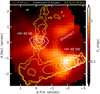 |
Fig. 1 Overview of the HH 48 system at MIRI wavelengths. The continuum-subtracted H2 V = 0-0, J = 5−3 line emission (9.66 μm) is shown in color tracing a complex structure of outflows and potential infall. The continuum at 5.24 μm is shown in white contours at 20, 60, 100, and 300 μJy, tracing the scattered light from the two protoplanetary disks. The [Fe II] line at 5.34 μm is shown in the yellow contours at 5, 10, 30, and 100 tracing the jets of both protostars. The primary, HH 48 SW, and secondary, HH 48 NE, are labeled in white. |
3 Observational results
An overview of the HH 48 system is presented in Fig. 1, in which we show the spatial extent of the continuum-subtracted H2 V = 0–0, J = 5−3 line with contours of the continuum at 5.24 μm (white) and the continuum-subtracted [Fe II] line at 5.34 μm (yellow). HH 48 is a binary of two T Tauri stars with a separation of ~2.″3 or 425 au. Both sources show extended con- tinuum emission at 5.24 μm. A jet is detected in both systems in the [Fe II] line emission at 5.34 μm. The noble gas lines from Neon and Argon exhibit a spatial distribution very similar to that of the [Fe II] lines, tracing the jet. The H2 emission (background in Fig. 1) extends far beyond the scattered light continuum and probably traces disk winds in both protoplanetary disks. Large- scale structure is detected in H2 toward the northwest of both sources that is not connected to any of the protostars in a coher- ent manner and traces the asymmetric structure earlier observed in CO J = 2 − 1 ALMA observations (see Fig. A.1 and Sturm et al. 2023c). This component only appears in low-energy H2 lines (Eup < 2000 K), which implies that the gas is cold with a high column density. A careful investigation of the region did not show any signs of an additional source, which means that the most likely origin of the large-scale structure is an infalling streamer feeding the system or an interacting large-scale wind. The focus of this paper is on HH 48 NE, as it is the more inclined of the two sources, but a spectrum of HH 48 SW is shown in Appendix B.
Figure 2 presents the source-integrated MIRI spectrum of HH 48 NE. Common gas emission lines are marked. Molecu- lar gas emission lines (e.g., CO, H2O) can be seen throughout the spectrum but will be analyzed in a future article, as the main focus of this paper is on the ice absorption features. The spec- trum shows a shallow silicate feature in absorption that peaks at 9.0 μm. The peak of this feature is offset compared to the peak observed in emission in systems with lower inclination (usually around 10 μm), due to an extra emission component from the inner disk that is scattered similarly to the continuum, as was also predicted by radiative transfer models (Sturm et al. 2023b). The observations are overall in good agreement with the photomet- ric data points compiled in Sturm et al. (2023c), except for the Spitzer/MIPS data point at 24 μm. This photometric data point was based on a 2D Gaussian fit to the low-resolution Spitzer data, which resulted in an overestimation by a factor of three.
To estimate the continuum baseline underneath the molecu- lar gas emission lines, we spline-fitted a line through the troughs between the lines including the broad features from PAH and ices in the continuum. Since the placement of this continuum is uncertain, all figures include the full data as well for comparison.
3.1 PAH emission
The most striking features are the PAH emission features most clearly seen at 6.23, 7.7, and 11.27 μm, but also at 5.4, 5.65, and 8.47 μm (see the PAH opacity template shown as the dashed line in Fig. 3, taken from Visser et al. 2007). The PAH emis- sion is spatially localized at the disk (i.e., we do not detect extended emission) and shows signs of severe wavelength depen- dent extinction since the 3 μm feature is absent and the 6.2 μm feature is weaker than expected. This suggests that the PAHs are located in the disk atmosphere and are obscured by its edge-on nature and/or that the UV/visible part of their excitation source is strongly attenuated. Given the uncertainty of the extinction, it is difficult to compare feature ratios to constrain anything about the PAH characteristics. The peak positions do not align with the established observational classes in ISM observations in Peeters et al. (2002) that usually correlate among different features; a potential combination of the three classes’ character- istics is observed concurrently, which is indicative of radiative transfer spectral modification or active PAH chemistry in the disk. Although the 12.6 μm feature is faint, it may be partially concealed by the H2O libration band (as is seen in the model without PAH in Fig. 3). The 5.4 and 5.65 μm features are more pronounced than anticipated compared to the 5.25 and 6.2 μm bands, possibly due to the presence of small PAHs with multi- ple hydrogen groups in trios (Boersma et al. 2009; Ricca et al. 2019). Further exploration of the origin and characteristics of the PAHs is required to elucidate their significance in the physics and chemistry of regions where planets are forming, extending the analysis to less massive stars like T Tauri stars.
3.2 Ice features
Strong ice absorption features, such as those observed in molec- ular clouds or protostars, are absent from our mid-infrared MIRI observations, which we interpret as a direct result of the multiple light paths that are possible through the disk (see for more details Sturm et al. 2023a). The strongest absorption feature is the CO2 bending mode at 15.5 μm with a peak optical depth of only 0.2. Due to the position of the PAH features and the effects of radia- tive transfer changing the profiles of the ice and silicate features, it is not appropriate to fit a polynomial to the continuum for ice identification and analysis. Therefore, a radiative transfer model tailored to this source is required to discriminate ice absorption features from silicate and PAH features.
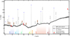 |
Fig. 2 Integrated MIRI spectrum of HH 48 NE. The continuum baseline underneath the gas emission lines is shown as a black line. Gas features are labeled accordingly. Molecular and recombination hydrogen lines are marked with colored tick marks. Absorption wavelength regions for important ices are marked on the bottom. Spitzer photometric data points are shown in red. |
3.3 Spatially resolved continuum emission in H H 48 NE
The left column of Fig. 4 presents the spatially-resolved contin- uum emission of the HH 48 NE disk at a range of wavelengths from optical HST observations to millimeter ALMA observa- tions. The bowl-shaped disk with a bright lobe on top, a dark lane, and a weaker lobe at the bottom, is recognizable up to 10 μm. The disk is spatially resolved up to 15 μm, which indi- cates that the continuum has a significant contribution from scattered light up to 15 μm. The east-west asymmetry that was observed previously in the optical HST observations is visible to a wavelength of ~ 10 μm. Normalized vertical and radial cuts through the continuum emission are shown on the right. Con- tributions due to HH 48 SW or possible dynamic interactions (Stapelfeldt et al. 2014; Sturm et al. 2023c) between the systems are masked in orange.
4 Model setup
Sturm et al. (2023a) show that the optical depth of the ice features in observations of edge-on protoplanetary disks is not linearly correlated with their column density and that the pro- files of the ice features can be significantly altered due to the scattering opacity of the ices. Since the disk is seen in scattered light in the JWST observations, it requires detailed 3D radiative transfer modeling to interpret the observed ice features and to constrain the region that is probed in the disk.
4.1 Physical structure
We adopted the model setup described in Sturm et al. (2023c,b). The input stellar spectrum was assumed to be a black body with temperature (Ts) scaled to the stellar luminosity (Ls). The density setup of the disk was parameterized with a power-law density structure and an exponential outer taper (Lynden-Bell & Pringle 1974),
![Mathematical equation: ${\Sigma _{{\rm{dust }}}} = {{{\Sigma _{\rm{c}}}} \over }{\left( {{r \over {{R_{\rm{c}}}}}} \right)^{ - \gamma }}\exp \left[ { - {{\left( {{r \over {{R_{\rm{c}}}}}} \right)}^{2 - \gamma }}} \right],$](/articles/aa/full_html/2024/09/aa50865-24/aa50865-24-eq1.png) (1)
(1)
where Σc is the surface density at the characteristic radius, Rc, γ is the power-law index, and e is the gas-to-dust ratio. The inner radius of the disk was set to the dust sublimation radius, approx- imated by  , and the outer radius of the grid was set to 300 au (1.″6), which is consistent with the observations of the disk extent.
The vertical structure of the disk is described as
 (2)
(2)
where h is the aspect ratio of the gas and small dust grains, hc is the aspect ratio at the characteristic radius, and ψ is the flar- ing index. We adopted two dust size populations to mimic dust settling in the system with a Gaussian distribution,
![Mathematical equation: ${\rho _{\rm{d}}} = {{{\Sigma _{{\rm{dust }}}}} \over {\sqrt {2\pi } rh}}\exp \left[ { - {1 \over 2}{{\left( {{{\pi /2 - \theta } \over h}} \right)}^2}} \right],$](/articles/aa/full_html/2024/09/aa50865-24/aa50865-24-eq4.png) (3)
(3)
where θ is the opening angle from the midplane as seen from the central star. The aspect ratio of the large grain population was restricted to X · h with X ∈ [0,1]. The fraction of the total dust mass that resides in the large dust population was defined as fℓ. The two dust populations followed a power-law size dis- tribution with a fixed slope of −3.5 between the minimum grain size, amin, and amax. amin and amax of the small grains were left as free parameters. The amin value is consistent across both grain populations, while the amax for the large grain population was fixed at 1 mm. The dust and ice opacities were calculated using OpTool (Dominik et al. 2021), using the distribution of hollow spheres (DHS; Min et al. 2005) approach to account for grain shape effects with fmax = 0.8. The gas was assumed to follow the small dust grain population, which implies that the gas-to-dust ratio varies over the vertical extent of the disk according to the dust settling.
The ALMA observations of HH 48 NE show clear signs of a central cavity, which is also supported by the spectral energy distribution (SED) and the HST scattered light observations (see Sturm et al. 2023c, for a detailed exploration of the source struc- ture). Therefore, we incorporated a basic cavity description by scaling the dust surface density of both dust populations within the cavity radius (Rcav) by a depletion factor (δcav); this can be seen in Table 1.
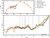 |
Fig. 3 Overview of the source-integrated spectrum of HH 48 NE (gray), with the continuum baseline underneath the gas lines shown in black with a zoom-in on the JWST wavelength range 2.7–27 μm. Different ice radiative transfer models are shown for comparison with the observations. The initial model constrained from photometric data points, HST, and ALMA observations (Sturm et al. 2023c,b) is shown in blue. A similar model was fine-tuned to the NIRSpec and MIRI spectrum with only refractory dust (red), dust and ice (green), and dust, ice, and PAHs (orange). The PAH opacity template used is shown at the bottom without extinction corrections (Visser et al. 2007). |
4.2 Ice distribution
The ices are initially distributed at a constant abundance with respect to hydrogen within the expected ice surfaces, with the initial abundances taken from the inheritance model in Ballering et al. (2021), based on observations summarized in Boogert et al. (2015). The model has an increasing number of ice species towards the midplane, based on their binding energy and a photodesorption limit. The thermal desorption ice line of each system was determined using the approach described in Hasegawa et al. (1992). The ice line is assumed to be at the point where there is more ice than gas available of a given molecular species
 (4)
(4)
where nice is the number density of molecules in the ice phase, ngas is the number density of molecules in the gas phase, ad is the characteristic dust grain size, nd is the dust number den- sity, S is the sticking coefficient which is assumed to be 1, kB is the Boltzmann constant, Τ is the dust temperature, Mn is the molecular mass of the species, Eb is the binding energy, Nss is the number of binding sites per surface area assumed to be 8 × 1014 cm−2 (Visser et al. 2011), and mi is the mass of the species, i. The region where ice is abundant is, in addition, ver- tically truncated by a limit that was initially put at AV = 1.5 mag, motivated by the onset of water ice in dark cloud observations (Boogert et al. 2015), which corresponds to z/r ~ 0.3. Inside and above this limit, the model consists of bare grains without ice mantles. This boundary is an approximation of the photodesorption limit and the slightly higher dust temperatures at low AV, which prevent ice formation on grains and assumes that all ice species are equally vulnerable to the same UV radiation.
In most parts of the disk, the vertical snowlines for H2O and CO2 were determined by this photodesorption limit; the verti- cal snowline for CO2 was set by thermal desorption only within ~20 au. For species such as CH4 and pure CO, which have lower binding energies, the vertical snowline was exclusively determined by thermal desorption.
The average density of the dust and ice composite was then calculated in every region using
 (5)
(5)
where x is the abundance with respect to total hydrogen, and M the mean molecular weight. The gas predominantly consists of H2 and He and has an abundance of xgas = 0.64 and a mean molecular weight of 2.44. The ice is distributed throughout the small and large grain population according to their surface area, assuming smooth spheres, following the description in Ballering et al. (2021),
 (6)
(6)
In each of the two dust populations, the ice is distributed over the grains assuming a constant dust core-ice mantle mass ratio assuming efficient dust growth in the disk after initial freeze out in early phases of the star forming process.
The additional mass of the ice was not added to the dust model, to keep the physical structure of the disk the same inde- pendent of the ice distribution. This implies that we effectively used a gas-to-solid ratio of 100 that includes silicates, amorphous carbon, and ice, instead of a gas-to-dust ratio of 100. Depending on the choice of definition of settling (dust only, or dust and ice) and gas-to-dust ratio, the actual ice mass can vary up to a factor of a few, a point we return to in Sect. 6.
Properties of the fiducial model presented in Sturm et al. (2023c,b) and the model tweaked to fit the JWST spectrum.
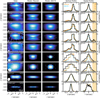 |
Fig. 4 Multi-wavelength spatial comparison between the models and the observations. First column from the left: the spatial appearance of the continuum emission from HH 48 NE in the optical HST observations, JWST MIRI observations, and millimeter ALMA continuum observations. Second and third columns: spatial appearance of the continuum emission from the fiducial model and MIRI fit, respectively, after convolution to a representative PSF. Last two columns: median averaged vertical and radial profile of the continuum emission normalized to the peak (black) with the fiducial model (orange) and MIRI fit (blue) on top. The orange box marks the region where HH 48 SW starts dominating the continuum. |
Properties of the ice retrieved in the models compared to the ISM.
4.3 PAHs
The spectrum shows clear signatures of PAH emission, as was described in Sect. 3, and without properly considering its emis- sion, it is difficult to identify and characterize the ice features.
The PAH emission is spatially localized to the disk, and the rela- tive strengths of the different features suggest that the PAHs are obscured, which means that they are emitting from within the protoplanetary disk. Therefore, we modeled the PAHs in a sim- plistic way, including a population of PAHs in the model using the opacities from Visser et al. (2007) assuming a size distribu- tion from 5 to 100 Å and a power law slope of 3.5. For the PAHs, we assumed the same temperature as for the dust; stochastic heat- ing by UV photons was not taken into account. The PAHs are limited to the regions in the model where ices are absent due to either thermal desorption or photodesorption. This assumption relies on the fact that PAHs are only excited in regions exposed to UV radiation and that their features are observed in emission rather than absorption. The mass of PAHs required to match the strengths of the features in the observations is 175 ppm of the disk mass, or 17% of the available carbon, which is consistent with ISM abundances and above previously modeled abundances that predict a depletion by orders of magnitude in Herbig Ae/Be stars (Sloan et al. 2005; Visser et al. 2007; Geers et al. 2009; Lange et al. 2023).
5 Modeling results
As a starting point, we adopted the physical structure from Sturm et al. (2023b). Initial ice abundances were established based on the average of their measurements relative to H2O ice in Boogert et al. (2015), with the H2O abundance at 8 × 10⁻⁵ following the reasoning in Ballering et al. (2021) and consistent with Sturm et al. (2023b) (see Table 2). This model is a good fit to the spatial extent of optical HST scattered light observations, ALMA mil- limeter continuum observations, and the SED (see Figs. 4, B.2 and Sturm et al. 2023c). The model reproduces the observed JWST spectrum reasonably well, except for the silicate feature and the flux at wavelengths >20 μm. The main reason for this is the change of origin of the continuum emission as, in the mod- els, the direct warm emission from the disk starts dominating over the scattered light of the warm inner disk in that particular region. Since the initial model is already close to the data, we perturbed the parameters of the fiducial model using the MCMC setup presented in Sturm et al. (2023c) with Ls, hc, ψ, Mgas, fℓ, amin, amax,s, and δcav as free parameters without waiting for conversion. The best-fitting model to the spectrum is given in Table 1 with only minor changes in the setup. Details on the out- come of the overall modeling and identified ices are presented in Sect. 5.1, and the effect of changing the size of the region in the disk where ices are included is investigated in Sect. 5.2.
5.1 Ice identification
In the NIRSpec spectrum (2.8–5.3 μm), we identified the major ice components H2O, CO2, and CO, and multiple weaker signa- tures from less abundant ices NH3, OCN−, and OCS and the 13CO2 isotopologue. Ice identification in the MIRI spectrum (5–28 μm) requires comparison with a model to correctly pre- dict the location of the ice features and to separate them from the PAH emission. Fig. 3 presents the comparison between the source-integrated spectrum of the observations and the best- fitting model including dust, ice, and PAHs (orange line). The model is overall a good representation of the spectrum with a few wavelength regions that are over-predicted.
5.1.1 H2O
The bending mode of H2O at 6 μm is present in both the obser- vations and the models, but is weak compared to the OH-stretch mode at 3 μm. Due to the PAH emission feature at 6.25 μm it is hard to tell whether the discrepancy between the model and the observations is a result of the continuum being slightly too high or if the feature is stronger in the observations than in the model; other molecules could contribute to the absorption feature. The libration mode of H2O at 12 μm is not observed in the spectrum, but the model without PAH emission (green vs. orange in Fig. 3) illustrates that the feature can also be hidden under the 11 and 12 μm PAH emission features.
5.1.2 CO2
The bending mode of CO2 at 15 μm is weaker than expected from the CO2 stretch feature at 4.3 μm (see Fig. B.2), and has the characteristic double-peaked profile of partially segregated CO2 ice (see e.g., Boogert et al. 2015, for a review). Partial segrega- tion indicates that heating has induced diffusion, resulting in the formation of isolated pockets of pure CO2 ice within the matrix. In addition, the bending mode has a broad contribution that is not accounted for in the model. The best-fitting model includes one component of CO2:CO at 20 Κ in a 3:1 ratio at an abundance of 6 ppm with respect to hydrogen. This ice mixture was chosen to accommodate CO being high up in the disk, and because it dominates the CO profile fit in Bergner et al. (2024). Using more mixtures could improve the fit to individual ice features in the MIRI range, but we refer to Bergner et al. (2024) for a detailed analysis of the ice profiles in the NIRSpec wavelength range. The models show that we can roughly reproduce the strength and shape of the CO2 feature and the CO feature with this single component. We revisit fitting the strength of both CO2 features in Sect. 5.2.2.
5.1.3 7 μm region
The 6.8 μm absorption feature commonly found in protostars and dark clouds, usually attributed to NH4+, is only weakly detected. Due to the PAH features at 6.25 μm and 7–9 μm, it is difficult to study this region in detail. However, the models suggest that there is an additional absorption feature centered at 6.8 μm that is currently not taken into account in the model, which could be due to the NH4+ complex (Keane et al. 2001; Boogert et al. 2008, 2015). Ice absorption features of other species, for example SO2 and CH4, are also known to occur at ~7.6–7.7 μm, the wavelength where the PAH feature is expected. The PAH feature shows a dent at the peak, which can be reproduced with the addition of CH4 ice to the model at ISM abundance (3.6 ppm, Ballering et al. 2021) with respect to hydrogen, but a component including, for example SO2, cannot be excluded (see Figs. 2, 5).
OCN− has a feature in this range as well and is weakly detected at 4.6 μm in the NIRSpec spectrum (Sturm et al. 2023a), but given the much weaker band strength at 7.6 μm, the contribution is most likely negligible (van Broekhuizen et al. 2004). Since the shape of the PAH feature is relatively unconstrained, we leave a detailed analysis of this ice feature to a future project.
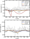 |
Fig. 5 Optical depth representation of the NH3 and CH3OH features (top) and the CH4 feature (bottom) with modeled features overlayed at different abundances. The black line indicates the continuum under- neath the gas emission features including ices. |
5.1.4 NH3 and CH3OH
Ammonia, NH3, is detected at 9.3 μm at a strength consistent with the feature found at 2.93 μm (see Fig. 5). This feature is reproduced with a component of pure NH3 in the model with an abundance of 0.5 ppm with respect to hydrogen, a factor 10 lower than the abundance assumed in the ISM. There is no clear sign of methanol, CH3OH, in the spectrum: there is no sign of the 9.7 μm CH3OH feature and the red wing of the H2O feature at 3.4 μm shows no sign of the narrow 3.53 μm CH3OH feature (Sturm et al. 2023a; Terwisscha van Scheltinga et al. 2018), even though it cannot be excluded that there is a minor contribution (cf. the discussion in Bergner et al. 2024). Given that the bind- ing energy of methanol is higher than that of CO2, this places tight constraints on the abundance in the disk regions that are traced with these observations. The maximum abundance of pure CH3OH in the model that is consistent with the observations is 0.5 ppm. We return to this in Sect. 6.
5.2 Localizing the measured ice
Due to the complex radiative transfer between the emission and detection of the light, our observations do not trace the bulk ice reservoir in the midplane of the disk. The presence of PAH emis- sion complicates this further. Furthermore, we have shown in Sturm et al. (2023a) that the spatially resolved information from the ice absorption is not directly related to the ice column density along the line of sight. The main reason for these results can be attributed to the position of the light source in our observations, which is situated at the center of the source rather than behind the disk as for background star observations. Consequently, we examine the ice characteristics along the multiple trajectories of the photons that scatter within the disk’s atmosphere, rather than along a narrow beam passing through the disk. In this section, we explore what regions our observations trace in the models, and constrain the region where the observed ices are located in the disk.
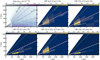 |
Fig. 6 Contribution function of the ice absorption features. Top left: total dust density distribution in the model with internal shielding (radial AV; dashed black line) at 0.03, 0.1, 0.3, 1, and 10 mag and external shielding (vertical AV; white dashed line) at 0.01, 0.03, 0.1, and 1 mag from top to bottom. The other panels show the contribution function (CBF), i.e., the contribution of a specific region to the total absorption of the ice feature in percentages. The pure CO ice at high abundance is added for reference, but we argue in the main text that this component is not observed. The absorbing area is the region in the disk that contribute significantly to the total absorption. The red and yellow lines indicate the fiducial and best fit photodesorption snow surface, respectively, for reference. The thick, dashed white line shows the τ = 1 surface at the ice feature wavelength. We would like to note that viewing angle is really important and is 83° in this case |
5.2.1 Contribution function
To constrain the region probed by our observations, contribution functions were generated for the ice absorption in the model. Due to scattering, it is not possible to deduce the regional contribu- tion from a single model, since it requires storing the complete trajectory of every emitted photon, which is not practical. There- fore, we rerun the same model multiple times, each time with the ices removed except for a specific region in the disk to test the contribution to the absorption in the source-integrated spectrum of that specific region. The disk is divided into five radial bins with edges at 0, 50, 100, 150, 200, and 300 au and 11 vertical bins at z/r of 0, 0.1, 0.15, 0.2, 0.25, 0.3, 0.4, 0.5, 0.6, 0.7, 0.8, and 0.9, which results in a total of 55 models. The course grid- ding is necessary to have sufficient S/N on the ice feature in the source-integrated spectrum in a reasonable computation time. It should be noted that we neglected photodesorption in this case to show what the contribution of ices to the total absorption would be at all positions in the disk. The regional contribution to the absorption of the different ice features in the source-integrated spectrum is displayed in Fig. 6. We included a model with one component of CO mixed in CO2 as given in Table 2, and a sep- arate model with one component of pure CO with a binding energy of 830 K.
By comparing the contribution functions in Fig. 6, we can identify three different categories. First, we see that the H2O and CO2 features in the NIRSpec wavelength range (3 and 4.3 μm, respectively) are dominated by a region between a radius of 50 and 100 au and significantly above the midplane (z/r = 0.2–0.5). The source of continuum at these wavelengths is the warm inner disk (Sturm et al. 2023b), scattered through the atmospheric lay- ers of the disk. Ice absorption is dominated by layers that are optically thin enough so that not all the light is absorbed but have enough ice mass to absorb a significant amount of light in the ice feature. The disk midplane is too optically thick to let pho- tons escape, and the disk atmosphere (z/r ≃ 0.5) and outer disk (r > 100 au) have too low ice mass to significantly contribute to the total absorption in the spectrum. There is a significant con- tribution from below the τ = 1 layer at the absorption feature wavelength (dashed white line), which is a result of the fact that a large fraction of the photons encounter multiple scattering and could scatter downward (cf. Sturm et al. 2023b,a).
Second, pure CO ice absorption would be dominated by a region in the model close to the midplane because of its physical location. Assuming a binding energy of 830 K (Noble et al. 2012) the pure CO ice is restricted to z/r < 0.15, which is reached by only a small fraction of the light. Due to the small fraction of light that reaches the CO ice-rich layer, the optical depths in the model cannot reproduce the data even for a very high CO abun- dance (c.f. Sturm et al. 2023b). Instead, CO is mixed with CO2 or H2O (see Sturm et al. 2023a and Sect. 5.2), leaving little room for pure CO (Bergner et al. 2024). CO mixed in the CO2 matrix shows similar results as the CO2 feature, which is no surprise given the small difference in feature wavelength.
Third, the CO2 feature at 15 μm traces a region close to the midplane between z/r of 0.1 and 0.15. The probed region with these features is closer to the midplane because of the longer wavelength of the features, which means that photons can pen- etrate further in the disk. Additionally, the dominant source of continuum changes at these wavelengths from scattering to ther- mal dust emission in the models (see Sturm et al. 2023b), which means that the layer with the highest density that is still opti- cally thin will produce the strongest absorption in the integrated spectrum.
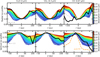 |
Fig. 7 Median averaged profiles of the peak optical depths in radial direction (top) and vertical direction (bottom). The data are displayed in black and models with varying vertical photodesorption threshold in z/r are shown in the colors specified in the colorbar. The dashed gray line shows the fiducial model with a photodesorption limit of AV = 1.5 mag and the dashed orange line indicates the vertical profile of the CO ice if pure CO ice is considered with a binding energy of 830 K. |
5.2.2 Locating elevated ices
There are three pieces of evidence indicating that the ices in the disk are elevated (located higher above the midplane) with respect to our model predictions assuming a photodesorption limit of AV = 1.5 mag. First, as is discussed in Sturm et al. (2023a), the vertical dependence on the absorption strength in the H2O, CO2, and CO features is less steep than expected if the ices were physically confined near the midplane. In Fig. 7, we present the median averaged dependence of the peak opti- cal depth as a function of both horizontal and vertical positions in the disk. These profiles are normalized to the absorption at r = 0 and z = 0. Unfortunately, the CO2 feature at 15 μm is not spatially resolved, and the signal-to-noise ratio for the other ice features is insufficient for a comparable analysis. To determine the vertical extent of the ices, we conducted simulations with different photodesorption limits based on an ice destruction con- straint in z/r. Subsequently, we convolved each wavelength point with the corresponding NIRSpec PSF using the WebbPSF pack- age (Perrin et al. 2012) and calculated the median dependence of the optical depth in both horizontal and vertical directions similar to the observations. The modeled profiles are depicted in Fig. 7. The gray line represents the standard model with a pho- todesorption limit of AV = 1.5 mag, while the colored regions display the outcomes for different desorption limits. Even with the standard photodesorption limit, there are absorption features at high altitudes (z > 50 au) caused by photons undergoing mul- tiple scattering events, although this is insufficient to account for the observed profile. The best-fitting model features a photodes- orption threshold of z/r = 0.6, corresponding to AV ~0.1 mag as observed from the star. The observed absorption profile for CO can only be explained by a component of CO mixed within a matrix with a higher desorption temperature, as pure CO is con- fined near the midplane due to its low desorption temperature, resulting in a sharp peak without a significant contribution from photons undergoing multiple scattering events (z > 50 au).
The radial profiles yield similar outcomes, although care has to be taken as these profiles are more sensitive to the source structure compared to the vertical profiles. One interpretation of our results would suggest that the CO2 feature aligns more closely with a photodesorption threshold of z/r = 0.5, and the CO feature with a photodesorption threshold of z/r = 0.4. How- ever, given the uncertainties, we assume similar snow surfaces for all three molecules.
The second piece of evidence for elevated ices in the atmo- sphere of the disk is the weak absorption of the bending mode of CO2 at 15 μm in comparison to the stretching mode at 4.3 μm. The intensity of the ice absorption feature correlates with the extent of the disk area impacted by ice absorption. The contri- bution function (shown in Fig. 6) indicates that the majority of the absorption at 4.3 μm originates from a height between z/r = 0.2–0.5, whereas the absorption at 15 μm is predominantly from regions near the disk midplane (z/r = 0.1–0.15). The standard model, with a photodesorption limit of AV = 1.5 mag, success- fully replicates the 15 μm bending mode but fails to predict the CO2 stretch mode at 4.3 μm by a factor of two (see Fig. 8). By expanding the region of absorption in the disk atmosphere by raising the photodesorption limit, the absorption at 4.3 μm increases significantly more than that at 15 μm, supporting a photodesorption limit at z/r = 0.6. Alternatively, increasing the abundance of CO2 in the model by about an order of magnitude in the z/r = 0.2–0.5 region, as probed by the 4.3 μm feature, could simultaneously account for both features with the fiducial photodesorption limit of AV = 1.5 mag. This would be consis- tent with some chemical models (e.g., Drozdovskaya et al. 2016; Arabhavi et al. 2022), but contradicts others (e.g., Ballering et al. 2021).
Finally, the shape of the ice features lends support to the notion of ice being located higher up in the disk because of geometric considerations. Apart from the importance of the extinction coefficient of ices, the refractive index of the ice also significantly influences the shape of the ice absorption features due to anisotropic scattering. In particular, additional absorption or emission wings are observed on either the blue or red side of the strong ice features (see also Dartois et al. 2022). In the NIRSpec observations of HH 48 NE, apparent emission wings are detected on the red side and absorption on the blue side of both the CO2 and CO features at 4.3 and 4.67 μm, respec- tively. This is opposite to the distortion observed in background star observations (e.g., Dartois et al. 2022; McClure et al. 2023; Dartois et al. 2024) because of the source structure. For obser- vations of background stars, the continuum is a consequence of direct emission from the star, and photons that scatter off the path on icy grains are not collected. However, for observations of disks viewed edge-on, the continuum is a result of scattered light, implying that photons that scatter from icy grains at a cer- tain angle might be included in the observations. These wings become more prominent when the photons scatter at extreme angles, indicating the presence of ice at higher elevations in the disk (see the sketch in Fig. 9). Figure 8 demonstrates that ice at z/r ~ 0.6 is required to explain the absorption at 4.18–4.21 μm and apparent emission at 4.29–4.4 μm.
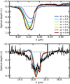 |
Fig. 8 Comparison between the 4.3 μm CO2 stretch feature and the 15 μm bending mode in the observations (black) and models with differ- ent vertical photodesorption limits (colored lines). The relative strengths of the features change with the photodesorption threshold due to a dif- ferent spatial origin of the absorption (see Sect. 5.2.1). The shape of the 4.3 μm and especially the red emission wing at 4.30–4.35 μm is also dependent on the height of the photodesorption limit due to geometric effects (see Fig. 9). No detailed fit to ice absorption profiles was per- formed, which could significantly improve the fit at 15 μm (see Bergner et al. 2024, for a fit of the 4.3 μm feature). |
6 Discussion
6.1 PAHs in edge-on protoplanetary disks
Protoplanetary disks that are observed face-on typically exhibit minimal or no indication of PAH emission, particularly within Τ Tauri star systems (see e.g., Geers et al. 2006; Visser et al. 2007; Henning et al. 2024). This absence is commonly under- stood to suggest a significant depletion of gas-phase PAHs by several orders of magnitude, combined with a lack of UV pho- tons to excite them for stars with a spectral type later than G8 (Geers et al. 2006; Tielens 2008; Geers et al. 2009; Maaskant et al. 2014; Lange et al. 2023). We find mounting evidence that edge-on systems regularly show strong 8 and 11 μπι PAH fea- tures (see also the spectrum of Tau 042021 in Arulanantham etal. 2024).
The fact that we see PAH emission in edge-on but not face- on disks suggests a localized origin of this emission. However, our best-fit model of HH 48 NE disk, if oriented face-on, still predicts strong PAH emission which is inconsistent with these previous observations (see Fig. 10). The way in which we imple- mented PAHs in the model is simplistic and did not include stochastic visible/UV excitation, but we expect the resulting dif- ferences to be minor (Woitke et al. 2016) and should not affect the conclusion that the PAH emission should be visible in face- on observations if they are equally distributed over the disk. However, this implies that the PAH abundance estimated from our model should be considered an upper limit. The inferred cav- ity in the HH 48 NE disk (Sturm et al. 2023c) might enhance the PAH emission due to reduced UV absorption by dust grains, thereby facilitating greater excitation of PAHs (Geers et al. 2009; Maaskant et al. 2014). Additional modeling is required to explain this dichotomy in the observations between the two inclination classes. Resolved observations of PAHs in edge-on and face-on systems would help constrain the properties of PAHs in disks (Lange et al. 2024).
Bright PAH emission significantly complicates the analysis of ice features, as they dominate the continuum between 6 and 10 μm. Therefore, we limit ourselves to the strongest ice features, and leave a search for the 6.8 μm NH4+ feature and potential complex organic molecule signatures at 7.2 and 7.4 μm (see e.g., McClure et al. 2023; Rocha et al. 2024) to a future study.
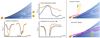 |
Fig. 9 Sketch of the three pieces of evidence for elevated ices in HH 48 NE. The orange line demonstrates the effect of including the ices high up in the disk on the vertical absorption profile (panel 1), the relative strength of the 4.3 to 15 μm CO2 features (panel 2), and the scattering wing of the 4.3 μm CO2 feature (panel 3). Two scenarios are proposed: a dusty disk wind blocking part of the UV emission from the star (Scenario A) or vertical mixing stirring up ice to the surface (Scenario B). |
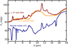 |
Fig. 10 Comparison of the fiducial model (blue; i = 83°) with face on disk models (i = 0°) at similar opacities with (red) and without (orange) PAHs. The PAH emission is predicted to be strong in the face-on case as well, which is contradictory to literature observations of less inclined Τ Tauri systems. |
6.2 Ices at high elevation in protoplanetary disks
We have shown using three different observables that at least part of the ice in HH 48 NE is located at a height of up to z/r = 0.6. The different methods are illustrated and explained in Fig. 9. Our snow surface for the main ice species is well above the photodesorption threshold of AV = 1.5, and is signif- icantly above the thermal desorption threshold for CO. As an additional check for the position of the snow surface, we ran thermochemical DALI models (Bruderer et al. 2012; Bruderer 2013) with the same physical structure and dust opacities as in the RADMC-3D model. This approach takes the full chemistry and molecular UV shielding (e.g., H2O lines) into account and is therefore a better representation than our simplified approach assuming a photodesorption cut-off based on dust extinction. We used the standard network that is based on the UMIST 06 net- work (Woodall et al. 2007) to solve for steady-state chemistry. Figure 11 presents the location of the snow surface, defined as the place where Xice = Xgas, for the three main ice species. The snow surface for H2O and CO2 in DALI is consistent with our simple parametrization of AV = 1.5 mag, and agrees well in the region between 50 and 100 au which is the dominant region that is probed by our observations (see Fig. 6).
We consider two scenarios that could explain why the ices are elevated above a molecule’s snow surface. In the first sce- nario, part of the UV radiation is blocked, possibly by a dusty wind that shields the ices in the disk’s atmosphere (see Fig. 9). Both a magnetically driven wind and a photoionized wind (Olofsson et al. 2009; Owen et al. 2011; Panoglou et al. 2012; Booth & Clarke 2021; Pascucci et al. 2023) do have the poten- tial to loft submicrometer-sized grains high into the atmosphere. We do see evidence of H2 emission above the disk that likely originates in a disk wind, and found that the disk atmosphere is poor in sub-micrometer-sized dust grains, which could be because they are actively transported away from the atmosphere by the wind (Sturm et al. 2023c). Additionally, the system has an inner cavity which is depleted in dust and gas, which could be a result of internal photoevaporation. In the case of a magnetohydrodynamic (MHD) disk wind, models suggest that a high accretion rate of 10−7 M⊙ yr−1 is necessary to sufficiently block the disk from UV radiation (Panoglou et al. 2012). Unfortunately, we do not have a reliable estimate of the mass accretion rate in the system because of the edge-on nature of the source, which blocks most of the emission coming from the inner disk. How- ever, considering the strong atomic jet and the potential streamer, it is not unlikely that the system is still strongly accreting. It has been proposed before that a dusty disk wind might account for the elevated AV values observed in a substantial sample of disks using the Ly alpha line, relative to the optical and infrared measurements (McJunkin et al. 2014). Further discussion on the implications and supporting evidence can be found in (Pascucci et al. 2023). UV shielding might also be increased by the appar- ently high concentration of PAHs in the warm regions of the disk (see Sect. 4.3), which effectively absorb UV radiation, or by molecular shielding from molecules like H2O (Bosman et al. 2022). If this scenario is true, it would have a significant impact on the interpretation of observations and models of protoplane- tary disks, as UV radiation is in many cases a dominant driver of the chemistry (e.g., Bergner et al. 2019, Bergner et al. 2021; Calahan et al. 2023) and can excite PAHs (Visser et al. 2007; Geers et al. 2009).
In an alternative scenario, the UV photons penetrate into the disk atmosphere as usual, but efficient mixing recycles the ices at higher altitude (see Fig. 9). Chemical modeling including ver- tical turbulent mixing and diffusion shows that icy grains can reach the observable disk surface in turbulent disks, effectively mixing ices upward faster than they can be photodesorbed in the upper layers (Semenov et al. 2006, 2008; Furuya et al. 2013; Furuya & Aikawa 2014; Woitke et al. 2022). The grain sizes of the icy grains inferred from the H2O and CO2 features (>1 μm; see Dartois et al. 2022 and Sturm et al. 2023a), which are thought to trace mainly the atmosphere of the disk, could be a direct result of mixing ice-rich micrometer-sized dust grains into the upper layers of the disk. If this scenario is the case, we expect to see enhanced effects of UV-driven chemistry in the outer disk as a result of UV reaching a significant fraction of the ices in the disk (Ciesla & Sandford 2012; Woitke et al. 2022), which could be tested with (sub-)millimeter (e.g., ALMA or NOEMA) observations.
Additional analysis on a larger sample of sources is required to constrain which of these scenarios is most likely. Future directions could involve including a better description of pho- todesorption and PAH excitation using the stellar UV field and interstellar radiation field, and including molecular shielding for example by H2O (Bosman et al. 2022). Currently, external radia- tion is disregarded based on the assumption that sufficient resid- ual cloud material shields the disk from such radiation; however, should it exert an influence, it would likely be counterproductive.
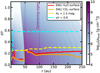 |
Fig. 11 Snow surface modeled with the simplified approach of AV = 1.5 mag (yellow) and the required height (cyan). The other lines indicate the snow surfaces of H2O (red) and CO2 (orange) in DALI models with a similar physical structure. The region that is predominantly probed by our ice observations (see Fig. 6) is marked with purple lines. |
6.3 Chemical implications
The molecular abundances that we need to include in the model to match the observations are listed in Table 2. The retrieved abundances relative to hydrogen are considerably reduced, up to ten times less, when compared to earlier results reported in Sturm et al. (2023a) and Bergner et al. (2024). This is a direct result from the elevated snow surface which spreads the ices needed to reproduce the observed line depths over a larger disk volume compared to the fiducial photodesorption limit. The presented abundances are a starting point for comparing observations with chemical models, including surface chemistry and vertical mixing. Our absolute abundances are in general lower than ISM abundances taken from the inheritance model in Ballering et al. (2021), this could be because we trace the ices in the disk atmosphere rather than in the midplane where the bulk of the ices reside. Combining multiple features of the same molecular species would allow us to study the ice composition and abundance in different regions of the disk; however, as is shown in Sect. 5.2.2 knowing the physical location of the snow surface beforehand is crucial as these properties are degenerate. Comparing the height of the snow surface derived with JWST with high resolution ALMA observations (for example of CO, H2CO, Podio et al. 2020) could help in this regard, but these are currently not available for this system. If sequestered ice is responsible for the gas-phase molecular depletion of CO and H2O (see e.g., Krijt et al. 2020; Sturm et al. 2022), then it is located in the midplane, where we cannot trace it with edge-on disk observations.
In Table 2, we compare the ice ratios with respect to water in the protoplanetary disk with the background star observations in McClure et al. (2023). The latter observations probe the ices in the molecular cloud stage in absorption against the contin- uum of a background star. Since the HH 48 NE observations are taken not far from the molecular cloud, the initial conditions of the disk were likely very similar to the background star obser- vations. The overall CO2/H2O column density ratio is consistent with the background star observations, although the individual mixtures have changed (Bergner et al. 2024). CO appears sig- nificantly less abundant in the protoplanetary disk, compared to background star observations. However, it is very likely that the disk observations only probe the CO that is trapped in the CO2 or H2O matrix and therefore survives high up in the disk, while the bulk of the CO ice is closer to the midplane where it can- not be probed by edge-on disk observations. CH4 is tentatively detected at the location of a PAH emission features, which makes the observed optical depth uncertain. Combined with the low binding energy, which indicates that the majority of the ice is located close to the midplane, the observed abundance is unre- liable. CH4 is expected to be abundant in protoplanetary disks due to the active carbon chemistry (Bruderer 2013; Woitke et al. 2016; Krijt et al. 2020; Oberg et al. 2023a), which is in line with the observations, but would be an order of magnitude higher than observed in comets and the ISM (see Table 2). Both NH3 and CH3OH are significantly depleted (×3 and >×3, respectively) in the disk with respect to the dark cloud (McClure et al. 2023). Both of these molecules are not efficiently formed in protoplan- etary disks, but predicted to be inherited predominantly from the natal cloud (Drozdovskaya et al. 2016; Ballering et al. 2021; Booth et al. 2021). Their low abundance suggests that at least part of the ice is reset and/or processed upon entering the pro- toplanetary disk. Alternatively, inherited ice ends up mostly in the midplane, and the ice we observe is formed locally in the disk. The low abundance of NH3 and CH3OH with respect to water is consistent with the observed abundances in comets. Pre- sumably, comets are formed in the midplane, so in the midplane the CH3OH abundance should be low as well, and thus favoring some reset. We would like to note, however, that comets trace the history of the protosun which may not have been formed in an environment like HH 48 NE, so one-to-one comparison is non-trivial and will require ice observations in a larger sample of disks around solar-like stars.
6.4 Limitations and future outlook
We have shown that we can approximately reproduce the NIR- Spec and MIRI spectrum with a relatively simple parameterized model including dust, PAHs, and ices. In this section we will discuss the main observables that can be used to constrain ice properties from the observations and give a future outlook to the possibilities.
6.4.1 Ice observables
Due to the complex radiative transfer in edge-on disk observa- tions, constraining properties of the ices is not trivial. Directly using the optical depth of the ice features to derive column den- sities can lead to errors of several orders of magnitude, which should be avoided (Sturm et al. 2023a). There are a few observ- ables that can be used to compare with models to learn more about the source structure, ice abundance and composition from the ice features.
The strength of ice absorption features is related to the size of the absorbing region in the disk and the ice abundance.
The vertical distribution of the peak optical depths of the ice can be used to locate ice vertically in the disk; In this work, we have shown that the ices in HH 48 NE are limited verti- cally by photodesorption, but a similar analysis can be done on thermal snow surfaces if, for example, pure CO ice is detected. Comparing the vertical dependence of the absorp- tion in the 15 μm CO2 feature with that of the 4.3 μm feature will give additional constraints on the source structure, as this will allow one to probe the extent of the absorbing area at this wavelength (see Fig. 6);
Modeling observations of multiple features from the same species (e.g., H2O and CO2) will enable the abundance and composition in different regions in the disk to be constrained. Moreover, their comparative intensities can serve as a gauge for determining the extent of the area that absorbs;
The isotopic ratios (e.g., 13CO2, 13CO) with the main isotopologue give information on the level of saturation in the main isotopologue, assuming a 12C/13C value. We have shown that our models can explain the strong 13CO2 absorption, but other isotopologues were unfortunately not detected. If, for example, 13CO had been detected, this would hint at a small absorbing area with a high abundance of CO instead of being mixed in CO2 and therefore widespread in the disk.
Ice profile shapes can be used to constrain the chemical envi- ronment of the ice which is done in a separate paper(Bergner et al. 2024). Combining multiple features can give insights into the vertical segregation of ice mixtures. This is only pos- sible with high spectral resolution mid infrared instruments like MIRI;
We have shown that scattering wings can be used to put con- straints on the source structure and the scale height of the ice, taking the geometry of the system into account. Addi- tionally, these features can be used to constrain the grain size distribution (cf. Dartois et al. 2022, 2024).
In the end, a combination of these observables will result in the best constrained source structure in the model and the best constraints on ice properties.
6.4.2 Future prospects
In this study, we have demonstrated the feasibility of fitting JWST observations using a relatively straightforward approach. All relevant observables discussed in Sect. 6.4.1 are simultane- ously matched in the model. Expanding the sample size is the next logical step to compare our results for HH 48 NE with other disks; currently, only this particular source has been thoroughly examined, and it may be an outlier due to its proximity to the companion HH 48 SW. The methodology employed presents a practical means to model a broader array of disks and gather data on the composition and distribution of ice in protoplane- tary disks. If other sources validate that the observed ices share a similar snowsurface as a result of photodesorption and ice mix- tures, a reasonable simplification in the fitting process is a model featuring only three dust populations: small dust particles with- out ice, small dust particles with ice, and large dust particles with ice. This streamlines computational efforts significantly and allows for further adjustments or the inclusion of ices in MCMC or χ2 fitting.
One drawback of using edge-on disks to investigate ices is that it does not capture the bulk of the ice mass in the disk mid- plane, but rather focuses on regions in the disk’s atmosphere (see Fig. 6). Disks with lower masses have the potential to reveal a higher proportion of their ice content, with features being less likely to be saturated. Nevertheless, observed edge-on disks typ- ically possess substantial mass by nature (Angelo et al. 2023), which complicates the analysis of ices.
If it is indeed the case that the contrast of the PAHs in the disk is intensified due to the high inclination of this source, iden- tifying subtle features will prove to be quite challenging. A more sophisticated incorporation of PAHs, including stochastic heat- ing, is essential to make any assertions regarding their abundance and distribution within the disk. Furthermore, future endeav- ors should focus on comparing the results with ALMA data to differentiate between various scenarios. The scarcity of high- resolution ALMA observations of molecules in edge-on disks necessitates further exploration to impose additional constraints on the physical disk structure and chemistry.
7 Conclusion
We presented new JWST/MIRI data to complete the ice inven- tory of the edge-on protoplanetary disk HH 48 NE. Radiative transfer models are fitted to the data to constrain abundances and the regions that are probed with the observations. We therefore conclude the following: - Edge-on disks are promising laboratories for studying ices in protoplanetary disks, as we find clear evidence for var- ious newly detected disk ice features including CO2, NH3 and tentatively CH4. JWST spectra can be fitted well with
3D radiative transfer models using a relatively simple setup, which enables detailed analysis of their abundance and physical location in the disk;
Ices are located unexpectedly high up in the disk, up to z/r ~ 0.6 and AV ~ 0.1. This result is determined based on the vertical dependence of the absorption, the ratio of the 4.3 and 15 μm CO2 features, and the scattering wings of the 4.3 μm feature. We suggest two possible scenarios: (1) Entrained dust in a disk wind is blocking the stellar UV radi- ation, so ice may survive higher up in the disk, but this would have strong implications for the gas-phase chemistry as well. (2) Alternatively, the icy material is efficiently elevated in the disk by vertical mixing, continuously replenishing the ice reservoir in the upper disk atmosphere;
JWST NIRSpec probes the ices in a higher layer in the disk than MIRI due to a change in scattering properties and the origin of the continuum. This complicates the analysis since the abundance and mixture of ices may change spatially in the disk, but with sufficient wavelength coverage, we can study multiple disk regions simultaneously.
The absence of a methanol feature and the faint NH3 fea- ture indicates that some of the ice from the original cloud is destroyed during earlier phases, reset upon entering the pro- toplanetary disk or remains concealed in the optically thick midplane;
The PAH emission contrast to the continuum is strong in HH 48 NE, but is extincted by the disk, which implies that it must be localized to the disk itself. Current models cannot explain why the contrast in edge-on systems is so much dif- ferent than in less inclined systems. This suggests that PAHs can be more abundant than previously thought, but only in specific regions in the disk probed by these observations. The spectrum of PAH emission bands hinders the analysis of ice features due to its strong, widespread impact on the continuum location.
JWST provides a unique opportunity to study ices and PAHs in protoplanetary disks in unprecedented detail. Full NIRSpec and MIRI coverage is required to understand and constrain the full ice inventory in protoplanetary disks. The application of the analysis presented here to additional protoplanetary disks will build a more global understanding of the composition and distri- bution of ices in these regions, which is important in the context of the evolution of planetary systems.
Acknowledgements
We thank the anonymous referee for the constructive feedback on the manuscript. Astrochemistry in Leiden is supported by the Netherlands Research School for Astronomy (NOVA), by funding from the European Research Council (ERC) under the European Union’s Horizon 2020 research and innovation programme (grant agreement No. 101019751 MOLDISK). M.K.M. acknowledges financial support from the Dutch Research Council (NWO; grant VI.Veni.192.241). Support for C.J.L. was provided by NASA through the NASA Hubble Fellowship grant No. HST-HF2-51535.001-A awarded by the Space Telescope Science Institute, which is operated by the Asso- ciation of Universities for Research in Astronomy, Inc., for NASA, under contract NAS5-26555. D.H. is supported by Center for Informatics and Computation in Astronomy (CICA) grant and grant number 110J0353I9 from the Ministry of Education of Taiwan. D.H. acknowledges support from the National Technol- ogy and Science Council of Taiwan through grant number 111B3005191. E.D. and J.A.N. acknowledge support from French Programme National ‘Physique et Chimie du Milieu Interstellaire’ (PCMI) of the CNRS/INSU with the INC/INP, co-funded by the CEA and the CNES. M.N.D. acknowledges the Holcim Foun- dation Stipend. Part of this research was carried out at the Jet Propulsion Laboratory, California Institute of Technology, under a contract with the National Aeronautics and Space Administration (80NM0018D0004). S.I. and E.F.vD. acknowledge support from the Danish National Research Foundation through the Center of Excellence “InterCat” (Grant agreement no.: DNRF150). M.A.C. was funded by NASA’s Fundamental Laboratory Research work package and NSF grant AST-2009253.
Appendix A Streamer
The H2 emission shows, apart from the disk winds in both sys- tems, an additional emission component to the North-West that is not correlated with the orientation of any of the sources’ out- flow. A comparison with the Moment 0 map of the CO J = 2 – −1 emission presented in Sturm et al. (2023c) shows that it is co-located with an asymmetric extension of redshifted CO emission, indicating that it is most likely an infalling stream of material falling on HH 48 NE. Unfortunately, the tail of HH 48 SW to the South-West is not observed because of the smaller MIRI field of view.
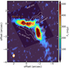 |
Fig. A.1 Overview of the asymmetric emission in the HH 48 system. The colored image shows the integrated CO J = 2 – −1 emission map of HH 48 NE (Sturm et al. 2023c). The contours indicate the spatial extent of the low energy H2 emission line at 9.67 μm. The ALMA beam (orange) and MIRI PSF size at 9.7 μm (white) are shown at the bottom right. |
Appendix B Spectral extraction
The source-integrated spectrum is extracted using a conical extraction, increasing the mask with wavelength according to the resolution, to get as much S/N on the spectrum as possible. To avoid contamination from the binary component, we used the mask of the primary source, HH 48 SW, as a negative mask on the mask for HH 48 NE (see Fig. B.1).
 |
Fig. B.1 Left: The integrated spectrum of HH 48 NE (red) and HH 48 SW (orange). NIRSpec data of HH 48 SW are not available as a result of the smaller field of view of the NIRSpec instrument compared to MIRI. Right: Continuum image of the HH 48 system at 24 μm with the masks used to extract the source-integrated spectrum shown on the left. |
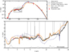 |
Fig. B.2 Same as Fig. 3 but with a comparison between the best-fitting model and the pre-JWST model published in Sturm et al. (2023b) |
Appendix C Model improvements
The current best-fitting model agrees well with the observed spectrum, with most discrepancies being less than 20%. This is an improvement over the model constrained pre-JWST (see Fig. B.2,4 for a comparison). There are a few instances where the model overestimates the flux (by less than 50%), particularly in the red wing of the water band at 3 μm. This overestimation could be due to an absorption component from ammonia hydrates (NH3H2O) around 3.5 μm, which is not accounted for in the model. The scattering wing in emission on the red side of the feature resembles the CO2 feature, further exacer- bating the difference. The regions around the silicate features (8–9 μm and 13–18 μm) are overestimated by 50%, possibly due to the source structure and the dust scattering characteris- tics in the system. The disk’s edge-on orientation suggests that the silicate features may have a scattered emission component from the warm inner disk and an absorption component from the cold outer disk. The ratio of these components is highly sensi- tive to the source structure, and they may not necessarily reflect similar grain compositions. The observations extending beyond the model’s spatial extent suggest that the model’s continuum source is mainly direct dust emission rather than scattered emis- sion, indicating a need for a higher placement of the scattering surface. An analysis using a two-component Gaussian fit to the radial profile of the continuum emission reveals a discrepancy in the ratio of scattering to direct emission between the mod- els (1:10) and the observations (1:2). While boosting scattering at these wavelengths is not straightforward, it likely involves a combination of source structure and grain composition. Investi- gating the inclusion of a third dust population with micron-sized grains in future studies could offer potential benefits. Maintain- ing a constant grain composition helps constrain the number of free parameters and speed up model computation. Future mod- els and JWST observations are expected to provide new insights into grain composition around silicate features, which can be leveraged to improve the model accuracy in the future.
Improvements can also be made by incorporating foreground cloud absorption in the modeling process. While the current model spectrum is scaled with the extinction curve based on AV, potential ice absorption in an envelope or foreground cloud is not considered. In particular models of younger sources may need to account for this. Uncertainties exist regarding the distribution of ices over dust grains, which can significantly influence measured abundances. The assumed system-averaged gas-to-dust ratio of 100 is consistent with most observations. Molecular abundances relative to hydrogen are integrated into the dust grains with- out altering the total mass in the region, effectively assuming an effective gas-to-solids ratio instead of a gas-to-dust ratio. Changes in the mass distribution can alter the physical structure and continuum significantly. Therefore, discussing ice-to-rock ratios in relevant disk regions is recommended over abundances when comparing with other systems due to the lack of precise constraints on the vertical gas distribution.
References
- Aikawa, Y., Kamuro, D., Sakon, I., et al. 2012, A&A, 538, A57 [NASA ADS] [CrossRef] [EDP Sciences] [Google Scholar]
- Angelo, I., Duchene, G., Stapelfeldt, K., et al. 2023, ApJ, 945, 130 [NASA ADS] [CrossRef] [Google Scholar]
- Arabhavi, A. M., Woitke, P., Cazaux, S. M., et al. 2022, A&A, 666, A139 [NASA ADS] [CrossRef] [EDP Sciences] [Google Scholar]
- Argyriou, I., Glasse, A., Law, D. R., et al. 2023, A&A, 675, A111 [NASA ADS] [CrossRef] [EDP Sciences] [Google Scholar]
- Arulanantham, N., McClure, M. K., Pontoppidan, K., et al. 2024, ApJ, 965, L13 [NASA ADS] [CrossRef] [Google Scholar]
- Ballering, N. P., Cleeves, L. I., & Anderson, D. E. 2021, ApJ, 920, 115 [NASA ADS] [CrossRef] [Google Scholar]
- Banzatti, A., Pascucci, I., Bosman, A. D., et al. 2020, ApJ, 903, 124 [NASA ADS] [CrossRef] [Google Scholar]
- Banzatti, A., Pontoppidan, K. M., Carr, J. S., et al. 2023, ApJ, 957, L22 [NASA ADS] [CrossRef] [Google Scholar]
- Bergner, J. B., Öberg, K. I., Bergin, E. A., et al. 2019, ApJ, 876, 25 [Google Scholar]
- Bergner, J. B., Öberg, K. I., Guzman, V. V., et al. 2021, ApJS, 257, 11 [NASA ADS] [CrossRef] [Google Scholar]
- Bergner et al. 2024, ApJ, submitted [Google Scholar]
- Boersma, C., Mattioda, A. L., Bauschlicher, C. W. J., et al. 2009, ApJ, 690, 1208 [NASA ADS] [CrossRef] [Google Scholar]
- Boogert, A. C. A., Pontoppidan, K. M., Knez, C., et al. 2008, ApJ, 678, 985 [Google Scholar]
- Boogert, A. C. A., Gerakines, P. A., & Whittet, D. C. B. 2015, ARA&A, 53, 541 [Google Scholar]
- Booth, R. A., & Clarke, C. J. 2021, MNRAS, 502, 1569 [NASA ADS] [CrossRef] [Google Scholar]
- Booth, A. S., Walsh, C., Terwisscha van Scheltinga, J., et al. 2021, Nat. Astron., 5, 684 [NASA ADS] [CrossRef] [Google Scholar]
- Bosman, A. D., Bergin, E. A., Calahan, J., & Duval, S. E. 2022, ApJ, 930, L26 [NASA ADS] [CrossRef] [Google Scholar]
- Boutéraon, T., Habart, E., Ysard, N., et al. 2019, A&A, 623, A135 [NASA ADS] [CrossRef] [EDP Sciences] [Google Scholar]
- Bruderer, S. 2013, A&A, 559, A46 [NASA ADS] [CrossRef] [EDP Sciences] [Google Scholar]
- Bruderer, S., van Dishoeck, E. F., Doty, S. D., & Herczeg, G. J. 2012, A&A, 541, A91 [NASA ADS] [CrossRef] [EDP Sciences] [Google Scholar]
- Brunken, N. G. C., Rocha, W. R. M., van Dishoeck, E. F., et al. 2024, A&A, 685, A27 [NASA ADS] [CrossRef] [EDP Sciences] [Google Scholar]
- Bushouse, H., Eisenhamer, J., Dencheva, N., et al. 2023, https://doi.org/10.5281/zenodo.8247246 [Google Scholar]
- Calahan, J. K., Bergin, E. A., Bosman, A. D., et al. 2023, Nat. Astron., 7, 49 [Google Scholar]
- Ciesla, F. J., & Sandford, S. A. 2012, Science, 336, 452 [NASA ADS] [CrossRef] [Google Scholar]
- Dartois, E., Noble, J. A., Ysard, N., Demyk, K., & Chabot, M. 2022, A&A, 666, A153 [NASA ADS] [CrossRef] [EDP Sciences] [Google Scholar]
- Dartois, E., Noble, J. A., Caselli, P., et al. 2024, Nat. Astron., 8, 359 [NASA ADS] [CrossRef] [Google Scholar]
- Dominik, C., Min, M., & Tazaki, R. 2021, OpTool: Command-line driven tool for creating complex dust opacities, Astrophysics Source Code Library, [record ascl:2104.010] [Google Scholar]
- Draine, B. T., & Li, A. 2007, ApJ, 657, 810 [CrossRef] [Google Scholar]
- Drążkowska, J., Alibert, Y., & Moore, B. 2016, A&A, 594, A105 [Google Scholar]
- Drozdovskaya, M. N., Walsh, C., van Dishoeck, E. F., et al. 2016, MNRAS, 462, 977 [NASA ADS] [CrossRef] [Google Scholar]
- Furuya, K., & Aikawa, Y. 2014, ApJ, 790, 97 [Google Scholar]
- Furuya, K., Aikawa, Y., Nomura, H., Hersant, F., & Wakelam, V. 2013, ApJ, 779, 11 [NASA ADS] [CrossRef] [Google Scholar]
- Geers, V. C., Augereau, J. C., Pontoppidan, K. M., et al. 2006, A&A, 459, 545 [NASA ADS] [CrossRef] [EDP Sciences] [Google Scholar]
- Geers, V. C., van Dishoeck, E. F., Visser, R., et al. 2007, A&A, 476, 279 [NASA ADS] [CrossRef] [EDP Sciences] [Google Scholar]
- Geers, V. C., van Dishoeck, E. F., Pontoppidan, K. M., et al. 2009, A&A, 495, 837 [NASA ADS] [CrossRef] [EDP Sciences] [Google Scholar]
- Habart, E., Natta, A., Testi, L., & Carbillet, M. 2006, A&A, 449, 1067 [NASA ADS] [CrossRef] [EDP Sciences] [Google Scholar]
- Hasegawa, T. I., Herbst, E., & Leung, C. M. 1992, ApJS, 82, 167 [Google Scholar]
- Henning, T., Kamp, I., Samland, M., et al. 2024, PASP, 136, 054302 [NASA ADS] [CrossRef] [Google Scholar]
- Jakobsen, P., Ferruit, P., Alves de Oliveira, C., et al. 2022, A&A, 661, A80 [NASA ADS] [CrossRef] [EDP Sciences] [Google Scholar]
- Kamp, I. 2011, in EAS Publications Series, 46, ed. C. Joblin, & A. G. G. M. Tielens, 271 [CrossRef] [EDP Sciences] [Google Scholar]
- Keane, J. V., Tielens, A. G. G. M., Boogert, A. C. A., Schutte, W. A., & Whittet, D. C. B. 2001, A&A, 376, 254 [NASA ADS] [CrossRef] [EDP Sciences] [Google Scholar]
- Kokoulina, E., Matter, A., Lopez, B., et al. 2021, A&A, 652, A61 [NASA ADS] [CrossRef] [EDP Sciences] [Google Scholar]
- Krijt, S., Bosman, A. D., Zhang, K., et al. 2020, ApJ, 899, 134 [NASA ADS] [CrossRef] [Google Scholar]
- Lange, K., Dominik, C., & Tielens, A. G. G. M. 2023, A&A, 674, A200 [NASA ADS] [CrossRef] [EDP Sciences] [Google Scholar]
- Lange, K., Dominik, C., & Tielens, A. G. G. M. 2024, A&A, 686, A181 [NASA ADS] [CrossRef] [EDP Sciences] [Google Scholar]
- Lynden-Bell, D., & Pringle, J. E. 1974, MNRAS, 168, 603 [Google Scholar]
- Maaskant, K. M., Min, M., Waters, L. B. F. M., & Tielens, A. G. G. M. 2014, A&A, 563, A78 [NASA ADS] [CrossRef] [EDP Sciences] [Google Scholar]
- McClure, M. K. 2019, A&A, 632, A32 [NASA ADS] [CrossRef] [EDP Sciences] [Google Scholar]
- McClure, M. K., Rocha, W. R. M., Pontoppidan, K. M., et al. 2023, Nat. Astron., 7, 431 [NASA ADS] [CrossRef] [Google Scholar]
- McJunkin, M., France, K., Schneider, P. C., et al. 2014, ApJ, 780, 150 [NASA ADS] [CrossRef] [Google Scholar]
- Min, M., Hovenier, J. W., & de Koter, A. 2005, A&A, 432, 909 [NASA ADS] [CrossRef] [EDP Sciences] [Google Scholar]
- Noble, J. A., Congiu, E., Dulieu, F., & Fraser, H. J. 2012, MNRAS, 421, 768 [NASA ADS] [Google Scholar]
- Noble, J. A., Fraser, H. J., Aikawa, Y., Pontoppidan, K. M., & Sakon, I. 2013, ApJ, 775, 85 Öberg, K. I., & Bergin, E. A. 2016, ApJ, 831, L19 [Google Scholar]
- Öberg, K. I., Facchini, S., & Anderson, D. E. 2023a, ARA&A, 61, 287 [CrossRef] [Google Scholar]
- Öberg, N., Cazaux, S., Kamp, I., et al. 2023b, A&A, 672, A142 [CrossRef] [EDP Sciences] [Google Scholar]
- Olofsson, J., Augereau, J. C., van Dishoeck, E. F., et al. 2009, A&A, 507, 327 [NASA ADS] [CrossRef] [EDP Sciences] [Google Scholar]
- Owen, J. E., Ercolano, B., & Clarke, C. J. 2011, MNRAS, 411, 1104 [NASA ADS] [CrossRef] [Google Scholar]
- Panoglou, D., Cabrit, S., Pineau Des Forêts, G., et al. 2012, A&A, 538, A2 [CrossRef] [EDP Sciences] [Google Scholar]
- Pascucci, I., Cabrit, S., Edwards, S., et al. 2023, in Astronomical Society of the Pacific Conference Series, 534, Protostars and Planets VII, ed. S. Inutsuka, Y. Aikawa, T. Muto, K. Tomida, & M. Tamura, 567 [Google Scholar]
- Peeters, E., Hony, S., Van Kerckhoven, C., et al. 2002, A&A, 390, 1089 [NASA ADS] [CrossRef] [EDP Sciences] [Google Scholar]
- Perrin, M. D., Soummer, R., Elliott, E. M., Lallo, M. D., & Sivaramakrishnan, A. 2012, SPIE Conf. Ser., 8442, 84423D [NASA ADS] [Google Scholar]
- Podio, L., Garufi, A., Codella, C., et al. 2020, A&A, 642, A7 [NASA ADS] [CrossRef] [EDP Sciences] [Google Scholar]
- Pontoppidan, K. M., Dullemond, C. P., van Dishoeck, E. F., et al. 2005, ApJ, 622, 463 [NASA ADS] [CrossRef] [Google Scholar]
- Pontoppidan, K. M., Stapelfeldt, K. R., Blake, G. A., van Dishoeck, E. F., & Dullemond, C. P. 2007, ApJ, 658, L111 [CrossRef] [Google Scholar]
- Pontoppidan, K. M., Salyk, C., Bergin, E. A., et al. 2014, in Protostars and Planets VI, eds. H. Beuther, R. S. Klessen, C. P. Dullemond, & T. Henning, 363 [Google Scholar]
- Ricca, A., Roser, J. E., Peeters, E., & Boersma, C. 2019, ApJ, 882, 56 [NASA ADS] [CrossRef] [Google Scholar]
- Rieke, G. H., Wright, G. S., Böker, T., et al. 2015, PASP, 127, 584 [NASA ADS] [CrossRef] [Google Scholar]
- Rocha, W. R. M., van Dishoeck, E. F., Ressler, M. E., et al. 2024, A&A, 683, A124 [NASA ADS] [CrossRef] [EDP Sciences] [Google Scholar]
- Rubin, M., Altwegg, K., Balsiger, H., et al. 2019, MNRAS, 489, 594 [Google Scholar]
- Schegerer, A. A., & Wolf, S. 2010, A&A, 517, A87 [NASA ADS] [CrossRef] [EDP Sciences] [Google Scholar]
- Semenov, D., Wiebe, D., & Henning, T. 2006, ApJ, 647, L57 [NASA ADS] [CrossRef] [Google Scholar]
- Semenov, D., Pavlyuchenkov, Y., Henning, T., Wolf, S., & Launhardt, R. 2008, ApJ, 673, L195 [NASA ADS] [CrossRef] [Google Scholar]
- Sloan, G. C., Keller, L. D., Forrest, W. J., et al. 2005, ApJ, 632, 956 [NASA ADS] [CrossRef] [Google Scholar]
- Stapelfeldt, K. R., Duchêne, G., Perrin, M., et al. 2014, in Exploring the Formation and Evolution of Planetary Systems, 299, eds. M. Booth, B. C. Matthews, & J. R. Graham, 99 [NASA ADS] [Google Scholar]
- Sturm, J. A., McClure, M. K., Harsono, D., et al. 2022, A&A, 660, A126 [NASA ADS] [CrossRef] [EDP Sciences] [Google Scholar]
- Sturm, J. A., McClure, M. K., Beck, T. L., et al. 2023a, A&A, 679, A138 [NASA ADS] [CrossRef] [EDP Sciences] [Google Scholar]
- Sturm, J. A., McClure, M. K., Bergner, J. B., et al. 2023b, A&A, 677, A18 [NASA ADS] [CrossRef] [EDP Sciences] [Google Scholar]
- Sturm, J. A., McClure, M. K., Law, C. J., et al. 2023c, A&A, 677, A17 [NASA ADS] [CrossRef] [EDP Sciences] [Google Scholar]
- Terada, H., & Tokunaga, A. T. 2012, ApJ, 753, 19 [NASA ADS] [CrossRef] [Google Scholar]
- Terada, H., & Tokunaga, A. T. 2017, ApJ, 834, 115 [NASA ADS] [CrossRef] [Google Scholar]
- Terada, H., Tokunaga, A. T., Kobayashi, N., et al. 2007, ApJ, 667, 303 [NASA ADS] [CrossRef] [Google Scholar]
- Terada, H., Tokunaga, A. T., Pyo, T.-S., et al. 2012, AJ, 144, 175 [NASA ADS] [CrossRef] [Google Scholar]
- Terwisscha van Scheltinga, J., Ligterink, N. F. W., Boogert, A. C. A., van Dishoeck, E. F., & Linnartz, H. 2018, A&A, 611, A35 [NASA ADS] [CrossRef] [EDP Sciences] [Google Scholar]
- Tielens, A. G. G. M. 2008, ARA&A, 46, 289 [NASA ADS] [CrossRef] [Google Scholar]
- van Broekhuizen, F. A., Keane, J. V., & Schutte, W. A. 2004, A&A, 415, 425 [NASA ADS] [CrossRef] [EDP Sciences] [Google Scholar]
- Visser, R., Geers, V. C., Dullemond, C. P., et al. 2007, A&A, 466, 229 [NASA ADS] [CrossRef] [EDP Sciences] [Google Scholar]
- Visser, R., Doty, S. D., & van Dishoeck, E. F. 2011, A&A, 534, A132 [NASA ADS] [CrossRef] [EDP Sciences] [Google Scholar]
- Walsh, C., Nomura, H., & van Dishoeck, E. 2015, A&A, 582, A88 [NASA ADS] [CrossRef] [EDP Sciences] [Google Scholar]
- Woitke, P., Min, M., Pinte, C., et al. 2016, A&A, 586, A103 [NASA ADS] [CrossRef] [EDP Sciences] [Google Scholar]
- Woitke, P., Arabhavi, A. M., Kamp, I., & Thi, W. F. 2022, A&A, 668, A164 [NASA ADS] [CrossRef] [EDP Sciences] [Google Scholar]
- Woodall, J., Agúndez, M., Markwick-Kemper, A. J., & Millar, T. J. 2007, A&A, 466, 1197 [CrossRef] [EDP Sciences] [Google Scholar]
- Yang, Y.-L., Green, J. D., Pontoppidan, K. M., et al. 2022, ApJ, 941, L13 [NASA ADS] [CrossRef] [Google Scholar]
All Tables
Properties of the fiducial model presented in Sturm et al. (2023c,b) and the model tweaked to fit the JWST spectrum.
All Figures
|
Fig. 1 Overview of the HH 48 system at MIRI wavelengths. The continuum-subtracted H2 V = 0-0, J = 5−3 line emission (9.66 μm) is shown in color tracing a complex structure of outflows and potential infall. The continuum at 5.24 μm is shown in white contours at 20, 60, 100, and 300 μJy, tracing the scattered light from the two protoplanetary disks. The [Fe II] line at 5.34 μm is shown in the yellow contours at 5, 10, 30, and 100 tracing the jets of both protostars. The primary, HH 48 SW, and secondary, HH 48 NE, are labeled in white. |
| In the text | |
|
Fig. 2 Integrated MIRI spectrum of HH 48 NE. The continuum baseline underneath the gas emission lines is shown as a black line. Gas features are labeled accordingly. Molecular and recombination hydrogen lines are marked with colored tick marks. Absorption wavelength regions for important ices are marked on the bottom. Spitzer photometric data points are shown in red. |
| In the text | |
|
Fig. 3 Overview of the source-integrated spectrum of HH 48 NE (gray), with the continuum baseline underneath the gas lines shown in black with a zoom-in on the JWST wavelength range 2.7–27 μm. Different ice radiative transfer models are shown for comparison with the observations. The initial model constrained from photometric data points, HST, and ALMA observations (Sturm et al. 2023c,b) is shown in blue. A similar model was fine-tuned to the NIRSpec and MIRI spectrum with only refractory dust (red), dust and ice (green), and dust, ice, and PAHs (orange). The PAH opacity template used is shown at the bottom without extinction corrections (Visser et al. 2007). |
| In the text | |
|
Fig. 4 Multi-wavelength spatial comparison between the models and the observations. First column from the left: the spatial appearance of the continuum emission from HH 48 NE in the optical HST observations, JWST MIRI observations, and millimeter ALMA continuum observations. Second and third columns: spatial appearance of the continuum emission from the fiducial model and MIRI fit, respectively, after convolution to a representative PSF. Last two columns: median averaged vertical and radial profile of the continuum emission normalized to the peak (black) with the fiducial model (orange) and MIRI fit (blue) on top. The orange box marks the region where HH 48 SW starts dominating the continuum. |
| In the text | |
|
Fig. 5 Optical depth representation of the NH3 and CH3OH features (top) and the CH4 feature (bottom) with modeled features overlayed at different abundances. The black line indicates the continuum under- neath the gas emission features including ices. |
| In the text | |
|
Fig. 6 Contribution function of the ice absorption features. Top left: total dust density distribution in the model with internal shielding (radial AV; dashed black line) at 0.03, 0.1, 0.3, 1, and 10 mag and external shielding (vertical AV; white dashed line) at 0.01, 0.03, 0.1, and 1 mag from top to bottom. The other panels show the contribution function (CBF), i.e., the contribution of a specific region to the total absorption of the ice feature in percentages. The pure CO ice at high abundance is added for reference, but we argue in the main text that this component is not observed. The absorbing area is the region in the disk that contribute significantly to the total absorption. The red and yellow lines indicate the fiducial and best fit photodesorption snow surface, respectively, for reference. The thick, dashed white line shows the τ = 1 surface at the ice feature wavelength. We would like to note that viewing angle is really important and is 83° in this case |
| In the text | |
|
Fig. 7 Median averaged profiles of the peak optical depths in radial direction (top) and vertical direction (bottom). The data are displayed in black and models with varying vertical photodesorption threshold in z/r are shown in the colors specified in the colorbar. The dashed gray line shows the fiducial model with a photodesorption limit of AV = 1.5 mag and the dashed orange line indicates the vertical profile of the CO ice if pure CO ice is considered with a binding energy of 830 K. |
| In the text | |
|
Fig. 8 Comparison between the 4.3 μm CO2 stretch feature and the 15 μm bending mode in the observations (black) and models with differ- ent vertical photodesorption limits (colored lines). The relative strengths of the features change with the photodesorption threshold due to a dif- ferent spatial origin of the absorption (see Sect. 5.2.1). The shape of the 4.3 μm and especially the red emission wing at 4.30–4.35 μm is also dependent on the height of the photodesorption limit due to geometric effects (see Fig. 9). No detailed fit to ice absorption profiles was per- formed, which could significantly improve the fit at 15 μm (see Bergner et al. 2024, for a fit of the 4.3 μm feature). |
| In the text | |
|
Fig. 9 Sketch of the three pieces of evidence for elevated ices in HH 48 NE. The orange line demonstrates the effect of including the ices high up in the disk on the vertical absorption profile (panel 1), the relative strength of the 4.3 to 15 μm CO2 features (panel 2), and the scattering wing of the 4.3 μm CO2 feature (panel 3). Two scenarios are proposed: a dusty disk wind blocking part of the UV emission from the star (Scenario A) or vertical mixing stirring up ice to the surface (Scenario B). |
| In the text | |
|
Fig. 10 Comparison of the fiducial model (blue; i = 83°) with face on disk models (i = 0°) at similar opacities with (red) and without (orange) PAHs. The PAH emission is predicted to be strong in the face-on case as well, which is contradictory to literature observations of less inclined Τ Tauri systems. |
| In the text | |
|
Fig. 11 Snow surface modeled with the simplified approach of AV = 1.5 mag (yellow) and the required height (cyan). The other lines indicate the snow surfaces of H2O (red) and CO2 (orange) in DALI models with a similar physical structure. The region that is predominantly probed by our ice observations (see Fig. 6) is marked with purple lines. |
| In the text | |
|
Fig. A.1 Overview of the asymmetric emission in the HH 48 system. The colored image shows the integrated CO J = 2 – −1 emission map of HH 48 NE (Sturm et al. 2023c). The contours indicate the spatial extent of the low energy H2 emission line at 9.67 μm. The ALMA beam (orange) and MIRI PSF size at 9.7 μm (white) are shown at the bottom right. |
| In the text | |
|
Fig. B.1 Left: The integrated spectrum of HH 48 NE (red) and HH 48 SW (orange). NIRSpec data of HH 48 SW are not available as a result of the smaller field of view of the NIRSpec instrument compared to MIRI. Right: Continuum image of the HH 48 system at 24 μm with the masks used to extract the source-integrated spectrum shown on the left. |
| In the text | |
|
Fig. B.2 Same as Fig. 3 but with a comparison between the best-fitting model and the pre-JWST model published in Sturm et al. (2023b) |
| In the text | |
Current usage metrics show cumulative count of Article Views (full-text article views including HTML views, PDF and ePub downloads, according to the available data) and Abstracts Views on Vision4Press platform.
Data correspond to usage on the plateform after 2015. The current usage metrics is available 48-96 hours after online publication and is updated daily on week days.
Initial download of the metrics may take a while.