| Issue |
A&A
Volume 698, May 2025
|
|
|---|---|---|
| Article Number | A8 | |
| Number of page(s) | 18 | |
| Section | Interstellar and circumstellar matter | |
| DOI | https://doi.org/10.1051/0004-6361/202452966 | |
| Published online | 23 May 2025 | |
The edge-on disc Tau 042021: Icy grains at high altitudes and a wind containing astronomical polycyclic aromatic hydrocarbons
1
Institut des Sciences Moléculaires d’Orsay, CNRS,
Univ. Paris-Saclay,
91405
Orsay,
France
2
Physique des Interactions Ioniques et Moléculaires, CNRS, Aix Marseille Université,
Marseille,
France
3
Leiden Observatory, Leiden University,
PO Box 9513,
2300 RA
Leiden,
The Netherlands
4
Space Telescope Science Institute,
3700 San Martin Drive,
Baltimore,
MD
21218,
USA
5
Jet Propulsion Laboratory, California Institute of Technology,
4800 Oak Grove Drive,
Pasadena,
CA
91109,
USA
6
Physikalisch-Meteorologisches Observatorium Davos und Weltstrahlungszentrum (PMOD/WRC),
Dorfstrasse 33,
7260
Davos Dorf,
Switzerland
7
Department of Astronomy, Boston University,
725 Commonwealth Avenue,
Boston,
MA
02215,
USA
8
Institute for Astrophysical Research, Boston University,
725 Commonwealth Avenue,
Boston,
MA
02215,
USA
9
Institute of Astronomy, Department of Physics, National Tsing Hua University,
Hsinchu,
Taiwan
10
INAF–Osservatorio Astrofisico di Catania,
via Santa Sofia 78,
95123
Catania,
Italy
11
Department of Physics, University of Central Florida,
Orlando,
FL
32816,
USA
★ Corresponding author: emmanuel.dartois@universite-paris-saclay.fr
Received:
12
November
2024
Accepted:
30
March
2025
Context. Spectra of the nearly edge-on protoplanetary discs observed with the JWST have shown ice absorption bands of varying optical depths and peculiar profiles, challenging radiative transfer modelling and our understanding of dust and ice in discs.
Aims. With the aim of constraining the underlying disc’s structure and evolutionary state, we build models including dust grain size, shape, and composition to reproduce JWST IFU spectroscopy of a well-characterised, massive, and large edge-on disc, Tau 042021. Specifically, we aim to match its spectral energy distribution, the spatial distribution of the dust and ice, and the spectral characteristics of the dust continuum and ice bands profiles, as well as test for the presence of astronomical polycyclic aromatic hydrocarbons (PAH) band carriers.
Methods. We explored radiative transfer models using different dust grain size distributions, including grains with effective radii of aeff = 0.005–3000 μm. Mass absorption and scattering coefficients for distributions of triaxial ellipsoidal grains were calculated using the discrete dipole approximation (DDA) for small size parameters (2πaeff/λ < 10), whereas the hollow sphere approximation was used for larger size parameters. We considered compositions including silicates, amorphous carbon, and mixtures of water, carbon dioxide, and carbon monoxide. The resulting orientation-averaged scattering matrices were input into RADMC-3D Monte Carlo radiative transfer models of Tau 042021 to simulate the spectral cubes observed with JWST-NIRSpec and MIRI. We compared the calculated optical depth distributions and profiles of the main ice bands to observations, including water at 3.05 μm, carbon monoxide at 4.67 μm, and carbon dioxide at 4.26 μm. We also compared these results to archival JWST-NIRCam and ALMA continuum images. We tested three increasingly complex disc structures, starting from a standard model and adding first an extended atmosphere, then a disc wind containing astro-PAHs.
Results. The observed near- to mid-infrared spectral energy distribution requires efficient scatterers, implying dust distributions that include grains of up to several tens of microns in size. The intensity distribution perpendicular to the disc exhibits emission profile wings extending into the upper disc atmosphere at altitudes exceeding the classical scale height expected in the isothermal hydrostatic limit. We produce ice absorption images that demonstrate the presence of icy dust grains up to altitudes high above the disc midplane, more than three hydrostatic equilibrium scale heights. We demonstrate the presence of a wind containing the carriers of astronomical PAH bands. The wind appears as an X-shaped emission at 3.3, 6.2, 7.7, and 11.3 μm, characteristic wavelengths associated with the infrared astronomical PAH bands. We associate the spatial distribution of this component with carriers of astronomical PAH bands that form a layer of emission at the interface with the H2 wind.
Key words: radiative transfer / scattering / solid state: volatile / planets and satellites: formation / protoplanetary disks / dust, extinction
© The Authors 2025
 Open Access article, published by EDP Sciences, under the terms of the Creative Commons Attribution License (https://creativecommons.org/licenses/by/4.0), which permits unrestricted use, distribution, and reproduction in any medium, provided the original work is properly cited.
This article is published in open access under the Subscribe to Open model. Subscribe to A&A to support open access publication.
1 Introduction
Nearly edge-on protoplanetary discs offer researchers the unique opportunity to trace the vertical distribution of dust and gas in a disc (e.g. Arulanantham et al. 2024; Duchêne et al. 2024; Sturm et al. 2023b,c; Dutrey et al. 2017; Guilloteau et al. 2016). However, at such a high inclination, the extremely high opacity towards the central nascent star prohibits direct line-of-sight observation of ices in absorption in the visible to infrared range. The observed spectra rather result from a complex radiative transfer as light scattered on the disc surface probes different parts of the disc. Spectral features thus carry signatures of the disc’s physical structure and of the different scattering properties of dust grains of various sizes, shapes, and compositions. With JWST, the dust and ice composition of nearly edge-on discs can be spatially resolved to reveal the chemical stratification of the (icy) dust grains. Recently, Sturm et al. (2024) studied the radial and vertical distribution of major ice species towards the edge-on disc HH 48NE. That work demonstrate that the retrieval of the spatial distribution of the ice is often non-trivial due to the complex photon propagation through the disc. The CO ice was observed at high altitudes similar to CO2 and H2O. Thorough radiative transfer models of icy dust grains are needed to infer both the ice and the dust grain distributions in the disc.
The Tau 042021 disc (RA 04:20:21.4, Dec +28:13:49.2; 2MASS J04202144+2813491), is a large and nearly edge-on (∼ 88∘) disc located in the nearby Taurus dense cloud (∼ 140 pc, Galli et al. 2019; Kenyon et al. 1994; Roccatagliata et al. 2020), first discovered in the visible (Luhman et al. 2009; Stapelfeldt et al. 2014; Villenave et al. 2020). Hubble Space Telescope Advanced Camera for Surveys (HST-ACS) observations further revealed the presence of a bipolar jet at 0.6 μm (Duchêne et al. 2014). The central star is estimated to be an M1 star (Luhman et al. 2009; Duchêne et al. 2024), with an effective temperature of ∼ 3700 K and a sub-solar bolometric luminosity. Along its major axis, the disc extends out to about 400–450 au in radius when observed in dust and gas in the visible and near-infrared (NIR), or with CO gas in the millimetre, whereas the millimetric (larger grain) dust emission is slightly less extended (Duchêne et al. 2024; Villenave et al. 2020, and references therein). It has recently been imaged in several infrared bands with the James Webb Space Telescope (JWST) by Duchêne et al. (2024), who analysed the images with refractory-only dust models, concluding that large ∼10 μm dust grains must be present and vertically well mixed with smaller grains. The large grains are found elevated to at least 60 au above the midplane at the largest disc radii. This observation implies that turbulence plays a crucial role, being strong enough to lift such large particles all the way to the surface of the disc. The paper also discusses potential sources of emission observed high above the midplane in their images, including the presence of a photodissociative disc wind that could entrain grains as large as ∼1 μm, producing a ‘veil’ of optical scattered light well above the disc midplane, and the possibility that PAHs or very small grains are entrained along with the gas and get stochastically heated once they reach high enough layers from which they are in direct sight of the central source. In contrast, ALMA dust continuum images show a significant degree of settling for larger grains probed up to the millimetre size range (Villenave et al. 2020, 2023).
In the first paper from the MIDAS JWST GO program (PID 1751), Arulanantham et al. (2024) used JWST MIRI spectroscopy to resolve the mid-infrared (MIR) spatial distribution of H2, revealing an X-shaped disc wind extending to ∼200 au above the disc midplane, as well as a bipolar jet arising from [Ne II], [Ne III], [Ni II], [Fe II], [Ar II], and [S III] forbidden emission lines. Extended H2O and CO gas emission lines are also detected, with excitation indicating that they arise from the central regions close to the star, but are scattered by the large dust grains in the disc surface. Finally, extended astronomical PAH band emission at 11.3 μm co-spatial with the scattered light continuum is observed.
In this article, we produce spatially resolved maps of ice absorption features in the Tau 042021 disc and use radiative transfer models to simulate them. In Sect. 2, we present the NIRSpec spectra and ice maps. Section 3 is devoted to the description of the physical model of the disc and describing how the icy grain properties are derived. A number of progressively complex physical models of spectra and ice maps are presented and compared to the data. The final section presents the conclusions of the study.
2 Observations
The observations presented here are part of the JWST Cycle 1 GO program ‘Mapping Inclined Disk Astrochemical Signatures (MIDAS)‘ (#1751, PI McClure). We observed Tau 042021 with NIRSpec on September 7 2023. The observations were taken with the G235H and G395H filters from 1.66–3.17 μm and 2.87–5.27 μm, respectively, at a spectral resolution of R∼2700, using the IFU observing mode with a pixel scale of 0.1′′ pixel−1 and a field of view (FoV) of 3.0′′ × 3.0′′. To fully capture the radial and vertical extent of this disc, predicted by our pre-launch radiative transfer models, we used a 2 × 2 mosaic and a four-point cycling pattern optimised for extended sources. Each cycled G395H exposure consisted of one integration of 25 groups with the NRSIRS2RAPID readout pattern for a total exposure time of 1518 s, while each cycled G235H exposure consisted of one integration of 5 groups with the NRSIRS2 readout pattern account, to account for data volume issues, for the same total exposure time of 1518 s. Since the regions surrounding Tau 042021 lacked bright stars in the field that could leak through the Micro-Shutter Assembly (MSA) failed open shutters and the intrinsic background emission is low at these wavelengths, we opted not to obtain either a leakcal frame or a dedicated background for these NIRSpec observations.
For MIRI observations, we refer to details presented in Arulanantham et al. (2024), of which we recall here only a brief description. These observations were taken on February 13, 2023 using a four-point dither pattern optimised for an extended source, with each dither exposure consisting of one integration of 69 groups, read using the FASTR1 readout pattern, for total onsource exposure times of 6594 s in each of the MIRI channels. A dedicated sky background was obtained with dithers of the same number of groups on a two-point dither pattern. Observations used the four different IFU channels, covering four wavelength ranges: 4.9–7.65 μm (Channel 1), 7.51–11.7 μm (Channel 2), 11.55–17.98 μm (Channel 3), and 17.7–27.9 μm (Channel 4). The smallest FoV and highest spatial resolution are available at shorter wavelengths in Channel 1 (3.2′′ × 3.7′′, 0.196′′ pixel−1). The FoV increases to 6.6′′ × 7.7′′ in Channel 4, and the spatial resolution drops to 0.273′′ pixel−1. For point sources, the average PSF FWHMs, denoted by theta in the subsequent equation, increase with wavelength, such that θ = 0.033(λ μm) + 0.106′′ (Law et al. 2023; Argyriou et al. 2023).
To supplement the MIDAS data and better constrain the physical model of Tau 042021, we gathered archival multi-wavelength images and spectra. The disc spectral energy distribution (SED) and HST/JWST/ALMA images were already modelled in Duchêne et al. (2024) using dust grains based on photometry and broadband images. We extend the range of the NIRSpec and MIRI data by adopting the photometric points from Table 4 in Duchêne et al. (2024). In the visible to NIR wavelength range, it is known that the scattered light from the disc shows significant variability over a period of a few days (Luhman et al. 2009). This is seen when comparing photometric points recorded at different periods to the JWST photometry. Some degree of variability in the flux is thus expected in the NIR if the data are not recorded at the same epoch.
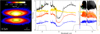 |
Fig. 1 NIRSpec observations of Tau 042021. Left: illustrative photometric image at 3.7 μm, showing the overall structure of the disc in continuum emission flux. Right: NIRSpec spectra of Tau 042021. The total flux integrated over both lobes is shown in black. The individual contributions of the upper emission lobe (red) and lower lobe (blue) are shown. The upper-to-lower lobe flux ratio is shown in gold. The ratio generally lies at around 2 across the continuum, whereas in some parts of the profile of the absorption bands, the lower lobe is more extinct than the upper. Some gaps in the spectra are due to the corresponding ‘gaps’ in the NIRSpec observations at some wavelengths. The photometry from NIRCam images presented in Duchêne et al. (2024) are shown in orange (the corresponding filter shapes for the NIRCam filters F200W and F444W are shown below in black). The corresponding photometry obtained by integrating the spectra over the same filter profiles from our work are shown in green. |
2.1 Observational extraction and analysis
NIRSpec datacubes provided by the JWST pipeline (1188 pmap version) were processed with in-house post-pipeline treatments, including routines to flag glitches by comparing sudden localised ‘hot’ pixels between adjacent channels, and interpolating the fluxes at the flagged spaxel positions. We applied a synthetic photometry approach to check the cross-calibration between NIRCam broadband images and NIRSpec IFU spectra. The NIRSpec spectro-photometry were compared to NIRCam by integrating through the F200W and F444W NIRCam bandpasses (Rieke et al. 2023), giving rise to photometric fluxes which agree well with Duchêne et al. (2024) photometric fluxes, as shown in Fig. 1. We extracted MIRI one-dimensional spectra by integrating over each lobe of the disc, after subtracting a background flux, estimated in an apparent empty region of the MIRI FoV. The spectra were scaled by 25% to the NIRSpec flux density in the overlapping region around 5 μm to account for potential differences in extraction aperture and compensate for intrinsic source variability. We construct optical depth images of the main ice bands by averaging the flux density of channels over 0.01 μm wide bins at the wavelength centre of each ice band. The optical depth of each spectral feature is derived by taking the ratio of the image at the ice band and an image at a continuum wavelength, chosen to be free of absorption. By taking an adjacent continuum point at a wavelength as close as possible to the ice band extinction, we take into account, as much as possible, the effects of propagation (and thus scattering) for similar wavelengths. This operation proceeds only for spaxels with intensities above a given threshold above the noise, defining the accessible dynamic range presented in the images. In particular, this means we cannot access the ice optical depth along the dark lane separating the two lobes. An optical depth map is derived as τ(x, y) = − ln (Fice(x, y)/Fcont(x, y)) to show ice spatial variations in ice distributions. If some photons are leaking from ice-free regions and contribute to the spectrum it adds an offset to the spectrum and implies the true optical depths might be higher. The important point is that these observed optical depth maps, as they will be compared to the models’ outputs, which are constructed in the same way, allow for a direct comparison between models and observations.
2.2 Images and spectra
Some NIRCam and MIRI images of Tau 042021 are shown in Duchêne et al. (2024) and the MIRI spectrum is shown in Arulanantham et al. (2024), where the gas phase lines are analysed. The opaque disc midplane divides the disc emission into two lobes with an approximate flux ratio of two between the upper lobe and the lower one, as expected for such a highly inclined disc (∼87.5∘). This is observed again in the left panel of Fig. 1, where we present an image in the continuum at 3.7 μm derived from the NIRSpec datacube by averaging fluxes in the cube channels over a 0.02 μm span around the central wavelength. The image is shown on a log scale, with the flux I normalised to the maximum (Imax) in the map. The scale is shown in the colorbar above and we can note that it covers almost two orders of magnitude.
The NIRSpec spectrum is presented in the right panel of Fig. 1. The emission from the two lobes is seen to maintain a relatively constant relative flux ratio of ∼2 across the spectrum. Strong ice absorption bands are evident in the spectrum of the disc, with the features dominated by the presence of H2O, CO2, and CO ices at 3.1, 4.26, and 4.67 μm, respectively. These are the major ice species expected to be present in ice mantles, and observed in other discs (e.g. Sturm et al. 2023b). Both lobe spectra and the total flux spectrum display similar overall features, and particularly have similar ice band profiles.
In the spectral region that overlaps with the observations of this disc by Pascucci et al. (2025), the fluxes we derive are in excellent agreement, and within potential source flux variations. As stated above, this disc scattering showed significant variability over a period of five days (see Fig. 10 in Luhman et al. 2009) and between different epochs in 2MASS (Cutri et al. 2003) 1.58 mJy at 2.2 μm, Spitzer, (Rebull et al. 2010) 2.1 mJy at 3.6 μm, thus up to 60% variation, a variability much higher than potential JWST photometric calibration issues. In the MIRI spectrum (Arulanantham et al. 2024, and Fig. 4), the main ice absorption feature observed is the bending mode absorption of CO2 at about 15.2 μm.
In addition to the ice bands, emission lines are observed superimposed on the continuum in both the MIRI spectrum (Arulanantham et al. 2024, and Fig. 4) and the NIRSpec spectrum in Fig. 1. Between about 4.3 and 5.3 μm, on top of the continuum, arise intense, high temperature gas-phase CO emission lines coming from the inner disc regions. In the MIRI range, astronomical PAHs emission shapes the spectrum in the 6 to 13 μm range. In this article, we refer to these observed emission features as the astronomical PAH bands. However, in the literature, these are often referred to as aromatic infrared bands, since the exact carriers are not identified (i.e. they have not been attributed to specific PAH). Some of the bands can definitively be attributed to the vibrational modes of aromatic species, and these features can also be referred to in the literature as ‘astroPAHs’, even shortened to ‘PAH emission features’. In this article, to distinguish the observed emission features from the carriers of the bands, we refer to astronomical PAH bands for the former and astronomical PAHs for the latter. When referring to model components used to reproduce both the emission and its associated carriers, we use the term astro-PAHs.
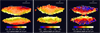 |
Fig. 2 Observed H2O, CO2, and CO ice optical depth mapped images of the disc at 3.0, 4.26, and 4.67 μm derived from the NIRSpec image at those wavelengths calculated relative to the reference continuum intensities taken at 3.7, 4.32, and 4.72 μm, respectively. Over-plotted white contours show the flux intensity at the band centres, normalised to their maximum in the map. The last contour is at 5% from the maximum. |
2.3 Optical depth imaging for H2O, CO2, and CO ices
Observed NIRSpec H2O, CO2, and CO optical depth mapped images of the disc at 3.0, 4.26, and 4.67 μm calculated against the reference continuum intensities taken at 3.7, 4.32, 4.72 μm, respectively are shown in Fig. 2. Over-plotted white contours show the relative intensities at the band centres – in the ice absorption – normalised to their maximum in the map. This shows the spatial extent of the dynamic range of the flux over which a meaningful optical depth could be derived. A gradient in the optical depth is seen in every ice band, but the optical depths for H2O, CO2 ices do not go to zero up to the sensitivity limit of JWST, and are still present very high in the disc atmosphere.
The first striking aspect is that the ice band optical depth images seem to extend far from the disc midplane and are comparable, in terms of spatial profile, to the adjacent continuum. We note that the vertical extension of the images presented here is limited by the achieved JWST signal-to-noise, and thus, even if a significant decrease were observed in the optical depth, ices might be present at even greater distances from the midplane. Indeed, if the CO optical depth asymptotically goes to zero in the outermost parts of the atmosphere, for H2O and CO2 ices the optical depth are still significant when the disc intensity goes to the limit of detection by JWST, and they thus could even extend slightly higher in the atmosphere than we have been able to measure here. The lower lobe absorbs slightly more due to the inclination, although we note that optical imaging shows that the brightness asymmetry between lobes is variable (Luhman et al. 2009).
2.4 Spectral signatures of scattering in ice absorption profiles
The ice band profiles are unusual when compared to those generally observed in dense clouds or protostars with the JWST (e.g. Yang et al. 2022; McClure et al. 2023; Federman et al. 2024; Le Gouellec et al. 2024), in particular for the CO2 ice bands. A spectrum with complete wavelength coverage from the north emission lobe of Tau 042021 in the NIR (i.e. excluding spaxels masked in the IFU at some wavelengths), scaled to the north lobe total flux at 3.7 μm, is shown in Fig. 3. It is compared to a dense cloud spectrum from Chamaeleon I, taken from McClure et al. (2023). The CO2 antisymmetric stretching mode around 4.26 μm in this almost edge-on disc is distorted, with a long extinction wing on the blue side of the profile and a sharp increase on the red side, just before the comb of gaseous CO emission lines. This is reminiscent of the profile inversion observed in recent NIRSpec observations of HH 48 NE (Sturm et al. 2023a) and several young objects with edge-on discs (FS Tau B, HH 30, IRAS 04302, including Tau 042021 analysed here, Pascucci et al. 2025). In contrast, the profile observed in the highly extinct source towards a dense cloud shows the opposite trend. Such characteristic profile modifications can be attributed to radiative transfer effects, including scattering with respect to dense clouds. In the case of protoplanetary discs, as is shown in, for example, Fig. 14 of Dartois et al. (2022), the emerging ice profiles will appear to be more affected than for spherical envelopes or dense clouds. These profiles can even be reversed with respect to dense cloud ones, with a pronounced blue-shifted wing absorption, and especially for a high inclination accompanied by high optical depths. Such profiles provide an important constraint on dust grains present in discs.
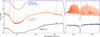 |
Fig. 3 Band profiles comparison. The integrated NIRSpec spectrum from the north lobe of Tau 042021, in a sub-region unaffected by NIRSpec IFU masking to fully sample the profile, is shown in red (multiplied by 1.2). It is compared to a typical dense cloud spectrum (NIRCam + NIRSpec IFU, black, flux (multiplied by two) observed at high extinction in Chamaeleon I (McClure et al. 2023). Note the inversion in the shape for the CO2 ice band profile around 4.27 μm betraying differences in radiative transfer properties. A laboratory transmittance spectrum (blue) of a H2O:CO2 ice film mixture used in the optical constants determination in Dartois et al. (2024) has been converted to flux scale for comparison. Spectra have been scaled to have similar optical depths in the ice absorption features in order to compare their profiles. |
3 Modelling and discussion
The observational data can be further interpreted with a series of models. We focus particularly on the description of the dust grains, including the presence of ice, accounting for the observed ice features, before discussing the implications of adding two main additional structural components – an extended dust grain atmosphere and a disc wind – to the standard disc structure.
3.1 Radiative transfer
To make relevant comparisons with the multi-wavelength SED, JWST spectra, and images, we performed radiative transfer calculations to model the expected spectra and images for Tau 042021. The calculations were performed using the Monte Carlo RADMC-3D1 software (Dullemond et al. 2012), utilising full anisotropic scattering for the dust radiative transfer. Details on the grain models used, both in terms of size distributions and physico-chemical composition, are given in the following sections. A spherical grid was used, and, taking advantage of the azimuthal symmetry, it was reduced to a radius and polar angle grid. The grid contains 256 radial points, spaced logarithmically in the radius from rin to rout, and sampled even more finely near the inner disc edge. The polar angle was sliced into 512 angles covering a total opening angle of 3π/4, centred on the disc midplane. After solving the radiative transfer, spectral cubes were produced at specific wavelengths with a FoV of 1000 × 1000 au, sampled with 5 au spaxels (200 × 200 pixels), adopting a pre-defined disc inclination.
3.2 Grain models
The approach adopted here for modelling observed spectra of such icy grains was detailed in Dartois et al. (2022, 2024). For a comprehensive understanding of the concept development, we refer interested readers to these references. Here, we provide an overview of the various stages involved, as well as the addition made to extend the size range of the dust size distribution to millimetre-sized grains. We define the grain shape and size distributions and the composition of the refractory phase within those grains, identify the composition of the ice phase, and structure the arrangement of refractory and ice components within the final grain structure.
Each mixed ice-refractory grain was modelled using the DDA programme DDSCAT (version 7.3, Draine & Flatau 2013). These grains are represented by dipoles with optical properties corresponding to both refractory and ice components, arranged stochastically to simulate a compact aggregate of smaller dust grains. This choice was driven by the expected stochastic sticking of dust grains from an initial smaller distribution, each coated with an ice mantle, representing the continuous process, from dense cloud to the disc phase, of ice mantle production and/or accretion onto grains, acting concomitantly with collisions, leading to the aggregation into bigger grains (e.g. Marchand et al. 2023; Lebreuilly et al. 2023; Silsbee et al. 2020; Paruta et al. 2016; Ormel 2014). Brief discussions of this choice can be found in Dartois (2006); Dartois et al. (2022). Laboratory-derived optical constants of ices and refractory materials were used, as is described in Dartois et al. (2022, 2024). From the available laboratory ice mixtures, we can determine the optical constants. The ice mixture composition that proves to be closest to the main ice absorption features observed, in other words the one most adequate for modelling Tau 042021, corresponds to a binary H2O:CO2 ice combined with a pure CO ice (previously used in Dartois et al. (2024). This choice has the additional advantage of showing how the radiative transfer affects differently the spectra in an edge-on disc when compared to a dense cloud line of sight, the latter discussed in Dartois et al. (2024), starting from the same set of optical constants. As dust grains exhibit non-spherical shapes, these add to the grain size in terms of contributing to scattering phenomena. To take this into account, we adopted a distribution of ellipsoids with many shapes represented by a weighted distribution of ellipsoid shapes exploring all the combinations of integers for the axis ratios within a factor of five (resulting in a total of 15 combinations). A discussion of this choice can be found in Sect. 2.2 in Dartois et al. (2022). In summary, such a distribution of ellipsoidal shapes explores a diversity of dust grains and, with such a weighting scheme, extreme shapes that have a non-physical probability of being present in space, such as when the ellipsoid tends to be like an infinite rod or to be planar, make a lower contribution to the distribution. The orientation-averaged cross-section was obtained by averaging over 16 orientation angles relative to the incoming plane wave for each ellipsoid. The DDA calculation is not suitable for calculating scattering and absorption cross-sections for very large values of the dimensionless size parameter x = 2πaeff/λ, where aeff is the effective radius of the grain and λ the wavelength under consideration. At large size parameters, the absorption and scattering cross-sections asymptotically converge towards their geometric regime. For size parameters above ten, we used the cost effective approximation given by a distribution of hollow spheres (dhs, Min et al. 2005), as implemented in the optool package (Dominik et al. 2021), to calculate the scattering and absorption cross-sections for smaller wavelengths (λ < 2πaeff/10). To ensure continuity between the calculations at their respective boundaries, the dhs parameter (corresponding to fmax, i.e. defining spheres with inner voids with volume fractions between 0 and fmax) was adjusted at the wavelength λ = 2πaeff/10 to match to the extinction cross-sections calculated with DDA and thus provide continuity.
The reference grain size distribution originates from the classical interstellar medium Mathis Rumpl & Nordsieck (MRN) distribution (Mathis et al. 1977), with grain radii ranging from aeff(min) of 5×10⁻³ μm to aeff(max) of 0.25 μm, hereafter denoted as amin and amax, respectively, for simplicity. The number density of grains of size a, between these limits, follows a power law. For each dust size distribution, grain growth is simulated by redistributing the total dust mass into a new size distribution characterised by a given amin and amax. Conserving the total dust mass thus redefines the slope of the power law in the distribution. This approach to grain growth parametrisation is consistent with numerous models’ outcomes of grain growth up to the protostellar phase (Marchand et al. 2022; Silsbee et al. 2020; Lebreuilly et al. 2019; Paruta et al. 2016; Ormel 2014; Weingartner & Draine 2001).
3.3 Dust grain components
The standard dust model used in our disc models has three main components corresponding to distinct physical regimes in the disc. The dust grain existence limit is first defined by the sublimation temperature of silicates, which is set here to 1300 K, corresponding to their typical sublimation temperature in discs (e.g. Kama et al. 2009). At lower temperatures, the three components are as follows:
- (i)
The first grain composition, modelled as bare grains of a mix of silicates and amorphous carbon, is set by where the grains are heated and/or exposed to UV. Bare grains are expected for temperatures above the ice sublimation limit, set at 100 K, and below the refractory (i.e. silicates set at 1300 K) sublimation limit. In addition, at temperatures below 100 K, if the UV flux is high enough, photodesorption hampers the in situ formation or re-accretion of a significant amount of ice. UV can come either from the central object or the exterior, so below a
 , applied both radially and vertically bare grains are assumed. In practice, the ice sublimation is often the dominant parameter defining the radial limit of this first grain composition. We shall return to the external UV field – that is, the vertical threshold – in the discussion.
 - (ii)
Another grain composition is defined below a visual extinction threshold, and where T < 100 K, where grains contain a combination of the previously mentioned refractory components and ices with a composition as defined above.
- (iii)
In the adopted dust grain size distributions, the largest grains start to decouple from the gas and progressively settle to the midplane of the disc (Villenave et al. 2020). To account for this, we thus implemented an icy dust composition with a larger grain size distribution, which has the same chemical composition as (ii), but located at a smaller scale height within the disc. The icy grain distribution is thus divided into two ranges. The first size distribution, for grains fully dynamically coupled to the gas, extends from amin to asettling, with a size distribution described by a power law adapted to preserve the total dust mass for an equivalent MRN distribution. This distribution’s boundaries are adopted to bare grains and the icy small- to medium-sized grains. Above this size limit are the settled grains, and this large grain distribution extends from asettling to 3 mm in size, the largest size limit in our calculations. The same power law is used for this distribution. An abundance factor is applied to the settled grain distribution to allow for a relative variation of large grains contribution with respect to the small- to medium-sized ones.
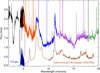 |
Fig. 4 Comparison of a combined NIRSpec (black) and MIRI (each channel is represented with a distinct colour: orange, blue, purple, or green) spectrum of Tau 042021 with spectra representing gas-phase contributions from CO gas (dark blue) and astronomical PAHs (brown) to the spectrum. See text for details. |
3.4 Gas phase CO and astronomical PAH bands treatment
Gas is included in the disc models as follows: a gas-to-dust ratio of one hundred is adopted, and the disc density is defined with respect to the gas distribution. In this section, we describe two components that present key spectral signatures in the observed data. A gas-phase CO component is particularly evident in the observed spectra, with CO lines spanning the ∼4.3 – 5.3 μm range, covered by NIRSpec (Fig. 4). We do not explicitly include the spectral signatures of this CO gas in the radiative transfer model. Figure 4 shows a simulated spectrum of gas-phase CO from the inner region at T ∼ 1500 K. Such a gas-phase contribution is produced in regions (r < 10 au and/or high above the disc surface; Salyk et al. 2011), which can be, to first order, decoupled from the core of the main (icy) disc radiative transfer model. CO gas is out of the main scope of this article and will be analyzed in future studies. The observed astronomical PAH bands emission spectrum from the HD97300 disc retrieved from the Spitzer archive (PID 2; Astronomical Observation Request 12697088, Low and High resolution), is also shown in Fig. 4. From the central positions and widths of the bands, it can be seen that the astronomical PAH bands from the HD97300 disc belong to a similar class of emission profiles as those in Tau 042021, thus allowing a first-order evaluation of their contribution to the SED. Astro-PAHs are not included in the first stages of the radiative transfer modelling, but will be discussed in a dedicated section below.
3.5 Standard disc structure
To analyse the observations, we used a series of disc models with increasing levels of structural complexity. We started with a classical, so-called ‘standard’ disc model, illustrated in the upper sketch of Fig. 5. The disc model is based on an axisymmetric flaring disc around a young star, described using classical parameters. The surface density of the disc is parametrised with
 (1)
(1)
where r is the radial distance to the star, r0 is a reference radius, and Σ0 the surface density normalisation at this reference radius. p is the power law exponent describing the radial variation, positive if the surface density decreases with radius. The density is tapered by an exponential edge with reference radius rt, following the viscous disc model theoretical solution (Lynden-Bell & Pringle 1974).
The vertical density distribution, under hydrostatic equilibrium, is given by
 (2)
(2)
with the density at the radial distance, r, and vertical distance, z, from the midplane. H(r) is the vertical scale height under a vertical isothermal hypothesis, whose radial variation is given by
 (3)
(3)
where H0 is the scale height at the reference radius, r0. h is the power law exponent describing the scale height radial variation, > 1 for flaring discs. The midplane density radial variation evolves thus with a power law as s = −(p+h).
The disc extends from its inner radius, rin, defined by the sublimation temperature of the refractory components to the outer radius, rout, which we set to 450 au, based on previous JWST and ALMA imaging (e.g. Villenave et al. 2020; Arulanantham et al. 2024), and a distance to the Taurus cloud of 140 pc (Kenyon et al. 1994; Roccatagliata et al. 2020; Galli et al. 2019). Rather than a sharp sublimation front, many discs possess an inner, less dense cavity filled with lower density of material. We added to the model the possible presence of an inner cavity, which then extends from rin to rcav, as is discussed in, for example, Sturm et al. (2023c), and which is only partly filled with grains by applying a δcav (< 1) factor to the prescribed densities for all the grain populations present at radii lower than rcav. To avoid overly sharp edges at the cavity boundary, the transition from the cavity edge to the δcav factor inside the cavity is tapered over a few percent of the cavity radius.
Millimetre images have also shown that large grains are progressively settling towards the midplane. To take into account this observed settling, the dust grain distribution is divided into two grain populations, one for small to medium grains and another one for large grains, as explained above. The large grain distribution possesses its own (over)density factor with respect to the small grain distribution, and its own (lower) scale height  . Each of these size distributions is homogeneous, and is well mixed within each zone.
The results of a standard model – with the main parameters close to the ones used in Duchêne et al. (2024); that is, Tstar = 3700 K, an inclination of 87.5∘, nH2 (100 au) = 1 × 109 cm−3, p = 0.7, rin = 0.07 au, rout = 450 au, and H0 = 7.5 au− are presented in Fig. 6 alongside observational data. The model includes, in addition, a lower-density cavity, rcav = 40 au, δcav = 0.05. The grain size distributions are set with amin = 1 μm, asettled = 40 μm, amax = 3000 μm, h = 1.2. The settled large grain scale height in this model 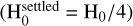 is less pronounced than that used previously (e.g. Villenave et al. 2020), due to the requirement for a slight asymmetry, which can be seen in the ALMA Band 7 image cut. The settled grain outer radius is also reduced compared to the small dust and gaseous disc, here 0.7 × rout, which is compatible with previous studies using a settled radius of about 300 au (Villenave et al. 2020; Duchêne et al. 2024).
The first striking difference between such a ‘standard’ model and the observations is the vertical extent of the disc, which is particularly evident at lower wavelengths. Even after the PSF convolution, the overall shape of these images possesses a rather flat-topped profile on each emission lobe. Standard hydrostatic models for almost edge-on discs will produce an intensity with an hourglass or chalice shape, as shown here and in many models presented in Fig. 13 in Duchêne et al. (2024). The morphology of the images observed for other edge-on discs – such as for HH30 with HST (e.g. Burrows et al. 1996) and, more recently, in NIRSpec continuum images around 4.65 μm (see Fig. 2 of Pascucci et al. 2025) or 2 μm (see Fig. 2 of Tazaki et al. 2025), in which the HH 30 hourglass shape of the continuum is clear and departs from Tau 042021 – seems adequately described with such an hourglass shape. Here, it is clear that in the JWST observations of Tau 042021 the intensities extend further out and the resulting observed intensity distributions look more like two ellipsoidal lobes in the NIR. This upper atmosphere of the disc can be seen in the vertical cuts through the disc centre shown in the right panels of Fig. 6, where the observed profiles are wider and extend further out than in the standard model.
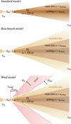 |
Fig. 5 Schematic edge-on views of the protoplanetary disc models used in this article. Upper panel: The ‘standard’ model includes a main disc flaring component with grains of sizes smaller than a critical size asettling and, possibly, settled dust grains for sizes above this size limit. The internal part of the disc (below rcav) can harbour a partially filled cavity (where the density is multiplied by a δcav < 1 factor). See Sect. 3.5 for details of the other parameters used in the ‘standard model’. Central panel: The extended atmosphere model, or ‘benchmark’ model, detailed in Sect. 3.6, supersedes the ‘standard’ model, while still including its main disc flaring component and settled dust grains. This model comprises an extended tenuous dust atmosphere lying above the classical purely hydrostatic model. Lower panel: The ‘wind’ model, detailed in Sect. 3.7.2, includes all the components from the benchmark model with the addition of a wind whose main parametrisation is shown here. Angles are given from the midplane axis. |
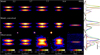 |
Fig. 6 Standard model. (upper) Model images at full resolution for selected wavelengths spanning the NIR to millimetre range. (middle) Model images once convolved with the JWST or ALMA PSF. (lower) JWST NIRSpec (2.2 and 3.7 μm), MIRI (7.7 and 14.4 μm), and ALMA Band 7 (890 μm) observations. Blue ticks are guides to the small wings observed at about 22.5∘, especially in the NIR, whereas brown tickmarks indicate an angle of 36∘ overplotted on the 7.7 μm image, corresponding to the angle for the X-shape discussed by Duchêne et al. (2024), and close to the H2 wind (semi-opening) angle previously observed in the 35–38.5∘ range by Arulanantham et al. (2024); Pascucci et al. (2025). The colorbars indicate the intensity levels, normalised to the maximum intensity for each image, in log scale except for ALMA data presented in linear scale. The right panel are cuts along the vertical line through the centre of the disc observations and models at the corresponding wavelengths (2.2 μm−blue; 3.7 μm-orange; 7.7 μm – purple; 14.4 μm – green, and 890 μm – brown). The spatial scale is expanded (shown with the black arrows) by a factor of two as compared to the images for a clearer view. The adopted blue-red-yellow color table was chosen to enhance the visibility of details in the structure. A version of this same figure with a uniform red temperature color table is presented in the appendix. |
3.6 Adding an extended atmosphere to the standard structure
From the results above, and as has already been concluded by Duchêne et al. (2024), it is evident that some grains are present high in the disc, producing a ‘veil’ of optical scattered light. This is evidenced when looking at the intensity perpendicular to the disc, as discussed above, with extended wings present well above the disc midplane and especially in the NIR. The standard radiative transfer with standard scale heights for small and large grain distributions, well describing the dominant mass fraction of the disc, must thus be modified to include the presence of small amounts of such grains. To consider this in the model, a small fraction of gas and grains can be present at a higher scale height than expected for the isothermal vertical density profile. The physical reasons for, and implication of the presence of, a tenuous extended atmosphere are discussed below.
The vertical density profile of an isothermal disc, defined using Eq. (2) implemented in the radiative transfer models described above, results in intensity profiles that are too narrow; that is, not extended high enough above the disc midplane. The observations clearly show a shallow intensity halo that is vertically extended, at several times the local scale heights (∼3 × H(r)) expected from a purely hydrostatic disc, due to an extended disc atmosphere. At such scale heights above the disc, departures from a pure Gaussian density profile are expected. There exist several physical reasons for that, including among the possibilities: deviation from pure hydrostatic equilibrium in relatively massive discs (and this disc must be massive given its large diameter approaching 1000 au), a non-isothermal temperature profile at large scale height (superheated layers), vertical diffusion, turbulence, the presence of dust ejected as a result of the left-over material from the recently imaged nested jets (Pascucci et al. 2025), or dust sustained at higher heights by the past or present remains of magnetic fields. Such departures have been proposed in previous models and discussed in general terms for many discs (Lee et al. 2024; Lebreuilly et al. 2023; Montesinos et al. 2021; Lesur 2021a; Armitage 2019; Dutrey et al. 2011; Hirose & Turner 2011; Ciesla 2010; Chiang & Goldreich 1997). Since, in the case of Tau 042021, we are dealing with an edge-on disc, it is more likely that we can see and probe such an extended upper atmosphere. To model the effect of an extended atmosphere, we adopt a simple configuration by slightly modifying the vertical density profile in a way that has been parameterised to empirically fit some of the protoplanetary disc models cited just above. We modify Eq. (2) by replacing it with the following extended atmosphere equation:
 (4)
(4)
The first term is the classical isothermal hydrostatic density profile from Eq. (2), while the second term produces a tail in the density profile corresponding to the extended atmosphere. Parametrising β as β = exp (−ϵ), for ϵ = {2, 5}, the extended atmosphere contribution surpasses the classical isothermal vertical density profile above a few z/h, as shown in the middle sketch of Fig. 5. Although it represents only a tiny fraction of the total dust mass, this extended atmosphere has a profound effect on the NIR intensity profile of the JWST images and spectra. The result of an extended atmosphere model calculation, similar to the standard model, but including the implementation of Eq. (4) with ϵ = 2.5, is shown in Fig. 9, and is referred to as the ‘benchmark model’ hereafter. This ϵ = 2.5 value allows the description of the vertical extent of the observed disc emission, especially in the NIRSpec wavelength range. As is shown in Fig. 7 it implies mobilising about or less than 1% of the disc dust surface density above three scale heights. Using this benchmark model including an extended atmosphere, we will try to reproduce the SED, the ice features’ spectral profiles, and the observed images in the following sections.
3.6.1 FIR/NIR SED provides global constraints on grain sizes
The extensive probe of all the possible parameters to be explored is a tricky aspect of disc modelling at such a level of detail. The calculation time required for the production of our RADMC3D models under full scattering radiative transfer being prohibitive, due to the need for high photon statistics considering the high level of scattering involved, we used a coarse grid of parameters for the size distributions with minimum size amin ranging from 0.005 μm to 10 μm, with the maximum size for this distribution, asettling from 0.25 μm to 100 μm. The upper size range is fixed to 3 mm for the largest grains. The scale height at the reference radius r0 = 100 au was varied between 6 and 10 au. The flaring index, h, was explored between 1.05 and 1.25. To narrow the parameter space to be explored in models, the intensity ratios in the observed SED of the source, in other words comparing millimetre emission to the NIR, as well as the slope in the MIR, provide constraints on the underlying and required dust distributions.
Based on the available photometric data, Duchêne et al. (2024) explored six different ice-free radiative transfer models, concluding that grains up to 10 μm in size are fully coupled to the gas up to the disc’s surface layers. In agreement with these results, we need a settled component of dust grains, and we explore hereafter the allowed range for this settling size. In addition, a better agreement is obtained for the ratio between the 20–50 μm range fluxes and the millimetre flux if we include a cavity that is a few tens of astronomical units in size. A 40 au cavity is close to the minimum cavity size necessary to match the 21 μm to 890 μm intensity ratio, with much lower cavity sizes producing an emission ratio in excess of what is observed. We explore in more detail the evolution of the intensity ratios with different models, including ices, and systematically varying amin and asettling, while setting the other parameters to values close to the midpoint of the previously explored parameter grid. This is shown in Fig. 8 for several models we calculated, concentrating on and starting from the benchmark model, then varying the amin and asettling values. A number of general trends have emerged from this parametric study. The essence of the results obtained is that the 2 μm over 890 μm intensity ratio first increases when asettling increases and then decreases. For amin larger than 2 μm, the decrease is pronounced. All models explored with asettling below a few microns failed to produce enough scattering intensity in the NIR with respect to the millimetre as observed. The same is true for distributions with asettling above about 50 μm. Models with asettling below a few microns also fail to produce the 2.0–4.4 μm ratio observed, with, for example, MRN-like distribution producing too steep a slope. The combination of just these two intensity ratios already restricts the parameters space.
Among the numerous parameters, based solely on the SED, the combinations of the NIR, MIR, and FIR ratios suggest that with a model comprised of two size distributions and including settling, the dust settling cutoff size should lie in the few tens of micrometres, whereas the smaller dust distribution minimum size must stay below a few microns, but be above the MRN cutoff as we need an efficient scatterer in the NIR to account for the 2μm/Flux (ALMA) flux ratio. A ‘benchmark’ model with these characteristics is discussed hereafter both in terms of distribution of intensities in images and spectroscopic ice band depths and profiles.
 |
Fig. 7 Vertical density profile for a scale height of H0 = 10, normalised to the midplane density, considering an isothermal model (solid line) and including an extended atmosphere as shown in Eq. (4) for ϵ = 2.5 (dotted line) and 4 (dashed line), corresponding to an atmosphere contributing above about 3–4 × z/h. The integral of the mass increase above 3 scale heights represents about 1 × 10⁻² of the total mass for ϵ = 2.5 and about 2 × 10⁻³ of the total mass for ϵ = 4, but strongly affects the radiative transfer in the upper layers. |
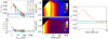 |
Fig. 8 Selected NIR-to-FIR characteristic intensity ratios. Left: intensity ratios calculated as a function of asetting for the benchmark model. amin, defining the evolution of the small and large dust grain distributions, is varied from the MRN value (0.005 μm) to 3 μm. The shaded regions delimited by dotted lines represent the expected observed intensity ratios, taking into account the variations between JWST observations and previous photometric data points. The central panels are 2D representations of the same model results. Right: exploration of the effect of cavity radius on the 21 to 890 μm intensity ratio in the benchmark model, which includes the presence of an inner, partially filled, cavity. A better agreement is obtained for rcav above several tens of astronomical units. |
 |
Fig. 9 Benchmark model, i.e. the ‘standard’ disc model plus an extended atmosphere. The nomenclature is the same as for Fig. 6. The presence of an efficient scatterer rather high up in the disc in this extended atmosphere allows for a better reproduction of the vertical distribution of observed intensities. See text for details. A version of this same figure with a uniform red temperature colour table is presented in the appendix. |
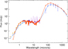 |
Fig. 10 Benchmark model spectrum (orange) overplotted on the SED data for Tau 042021, normalised to the observed average flux in the NIRSpec range. Blue photometric points are taken from Table 4 of Duchêne et al. (2024). Orange symbols correspond to the ≤ 2.2 μm photometric points adjusted by a factor to match the JWST flux, taking into account the known potential variability of the source (see text for details). Error bars (3σ) are given for the long wavelength photometric points from Spitzer/MIPS, Herschel/PACS and Herschel/SPIRE, retrieved from published point source catalogues. |
3.6.2 Images at relevant wavelengths
The benchmark model fulfilling the characteristics constrained from our simple SED analysis is shown in the first row of Fig. 9, at selected wavelengths spanning the NIR, MIR, and the submillimetre from ALMA Band 7. The wavelength selection from the model covers continuum emission wavelengths from the disc, avoiding strong ice bands. The second row of images, obtained by convolving the simulated images with the Webb PSF (ALMA PSF for the last image) at each corresponding wavelength can then be compared to the observations presented in the lower row of the figure. The consequence of the presence of an efficient scatterer rather high up in the disc (above about 3 scale heights), which motivated the addition of an extended atmosphere, is obvious when compared to the standard model images from Fig. 6. It better describes the distribution of intensities as observed with JWST images of the Tau 042021 disc. As shown in the rightmost column – which compares the intensity profiles of cuts passing through the centre of the disc along the perpendicular axis – with this extended model, the intensity wings extending up to the upper disc atmosphere are better reproduced than the standard model without the extended atmosphere. Despite this overall improvement, the central image, at 7.7 μm, still departs significantly from the model, which suggests it requires an additional component.
The SED calculated from the modelled images is shown in Fig. 10, and a detailed zoom of the NIRSpec-MIRI range is shown in Fig. 11. The global agreement is good, albeit with a remaining excess still present around 100 μm and below 0.5 μm. The excess at long wavelength might be due to deviations of the underlying optical constants in the model from the true optical properties of the grains, whereas the excess in the UV-visible below 0.5 μm most probably arises from an accretion driven mechanism that we do not include and thus cannot reproduce in the modelling.
The observed optical depth images first presented in Fig. 2 are now compared in Fig. 12 to the optical depth images resulting from the extended atmosphere benchmark model. We qualitatively reproduce well both the absolute values of optical depth and their spatial evolution across the disc except for lines of sight directly aligned perpendicular to the pole close to the stellar line of sight. In particular, there is a pronounced high optical depth ridge at the terminator separating the dark disc from the start of bright emission, and a sort of valley with a progressive decrease moving upwards until the disc emission becomes too low to be measurable. In the models, as in the observations, the ice band optical depth images extend far from the disc mid-plane and are comparable, in terms of spatial profile, to the adjacent continuum (see Fig. 9). We do not see and measure a sharp frontier for a transition to a sublimating zone for H2O and CO2 ices in the observations, they are present everywhere that we can measure. Only the CO optical depth seems to asymptotically reduce to zero in the outermost parts of the atmosphere at some point. This suggests that ices observed in the upper atmosphere of the vertical density profile are sufficiently well protected both from VUV photons external to the cloud, and from direct illumination of the source (shielded by the innermost grains), otherwise they would have been desorbed, or, dragged or entrained into the upper atmosphere (relatively recently).
3.6.3 CO2 profile
The profile of the antisymmetric stretching mode of solid CO2 observed in the Chamaeleon cloud against background sources, in other words in direct extinction (e.g. McClure et al. 2023; Dartois et al. 2024), tends to form an asymmetric profile with a band exhibiting excess extinction in the red wing and – because the dust grain size at the upper bound of the size distribution reaches micron sizes – shows an apparent slight flux increase on the left, towards shorter wavelengths. In contrast, the observation of solid CO2 in protoplanetary discs, observed at a relatively significant degree of inclination, associated with high optical depths and subject to radiative transfer effects, often reveals a profile that appears inverted, with a pronounced blue wing that can extend relatively far from the core of the band absorption (e.g. IRAS04302+2247, Aikawa et al. 2012, Fig. 3; Pascucci et al. 2025) and such a profile inversion is observed in the case of Tau 042021 (this work, Pascucci et al. 2025) and other discs such as HH 48 NE (Sturm et al. 2023b; Bergner et al. 2024), FS Tau B and HH 30 (Pascucci et al. 2025).
The ice band profiles in this work, including the pronounced CO2 feature blue wing extinction, provide constraints on the range of parameters for the models. This is especially true for the CO2 band, because, for a solid phase absorption band, it is intense and narrow. Additionally, it falls in a region of the spectrum fairly free of competing features. The inversion of the CO2 profile, which is reproduced in our benchmark model, as shown in the model overplotted over the observations in Fig. 11 provides a stringent spectral constraint on the models.
3.7 Testing the presence of a wind containing astro-PAHs
3.7.1 Observational constraints
As was mentioned above, and highlighted by the study of the 7.7 μm emission, the ‘benchmark’ model – the model with an extended atmosphere – is (in some of the images) insufficient to explain the spatial distribution of the intensity. An X shape is observed to emerge from, and extend beyond, the smooth and progressive evolution of the disc images attributable to the (icy) dust grain bands and continuum alone. A peculiar X-shaped feature is already observed in broadband NIRCam and MIRI imaging at 7.7 and 12.8 μm and discussed by Duchêne et al. (2024). This feature is absent from their other images at 2.0, 4.4 and 21.0 μm. An H2 wind has been identified from line images constructed for H2 rovibrational transitions from spectral observations with MIRI and NIRSpec, and discussed in Arulanantham et al. (2024) and Pascucci et al. (2025), respectively. The H2 transitions, because of their high fluxes, also contribute to the previous wide-band sensitive images, as well as other potential components, and this is where constructing narrower band images from the IFU spectral data can help in discriminating the carriers. Some IFU images in the MIR require the existence of an additional component to explain the observations. As these structures could follow the wavelengths characteristic of the emission linked to the astronomical PAH bands (e.g. Chown et al. 2024; van Diedenhoven et al. 2004; Peeters et al. 2002; Leger & Puget 1984; Allamandola et al. 1985), whose prominent bands are expected around 3.3, 6.2, 7.7, 11.3 μm, we produced filtered images in dedicated bands corresponding to these features to demonstrate this. Guided by the MIRI integrated disc spectrum of Tau 042021 as shown earlier in Fig. 4, we have averaged several spectral images in a wavelength band around positions crucial for determining the contribution of the astronomical PAH bands, and did the same for nearby wavelengths to sample the adjacent continuum disc emission outside these bands. We also selected nearby wavelength ranges with intense H2 transitions to compare them to the expected structure associated with the already identified H2 wind. The ‘line or band filter’ wavelength ranges are shown in Fig. 13, for NIRSpec (left) and MIRI (right) while the corresponding images constructed from these filters are shown in Fig. 14. The bands of interest to be cross-compared, on which these filters have been positioned, are at 3.28, 6.25, 7.7, and 11.3 μm to monitor the astronomical PAHs emission bands, and 3.325, 6.909, 9.667 μm for H2, corresponding in the case of the latter to the H2 1–0 O(5), H2 0–0 S(5) and 0–0 S(3) transitions, respectively. Continuum images have been prepared for NIRSpec from filters at 3.21 and 3.35 μm (to estimate the continuum baseline to be subtracted from the 3.28 μm astronomical PAH band corresponding to the CH stretching mode). For MIRI, filters were placed at 5.8 and 10.25 μm to monitor the continuum outside, but sufficiently close to, the astronomical PAH bands centred at 6.25, 7.7, and 11.3 μm. In the MIRI range, the spectrum of astronomical PAH emission bands in another disc (HD 97300) observed with Spitzer (retrieved from the Spitzer archive as explained previously) is plotted below Tau 042021 to show that the chosen continuum wavelength positions fall in minima with respect to the astronomical PAH bands. These filters are used to estimate and properly subtract the other components in the disc (i.e. the ice features and dust continuum emission) contributing to the astronomical PAHs images. The bottom row of Fig. 14 shows the distribution of intensities for continuum-subtracted astronomical PAH bands observed at 3.28, 6.25, 7.7, and 11.3 μm. There is evidence of an X shape in each of the three bands. This shape is already seen in the raw images (i.e. not yet continuum-subtracted) at 6.25, 7.7, and 11.3 μm, although the contrast is much higher when the continuum filter contributions are removed. At 3.28 μm, the contrast is far less intense, and the PAH astronomical band does not appear to be present in the raw image, but becomes evident upon continuum subtraction. When the images fall at wavelengths corresponding to astronomical PAH bands in the MIRI range, the shape of the emission contrasts with the rounded, less extended, shape of the ice and/or dust continuum, confirming that the astronomical PAHs are the most probable carriers of this X-shaped emission.
Another result of this analysis, obtained by comparison with the H2 emission bands, is that this astronomical PAHs-related X-shaped distribution of intensity is much more angularly extended than the H2 wind. The width and opening angle for the X shape seems more open than that observed for the H2 emission lines tracing the H2 wind, the latter appearing to be nested in this astronomical PAH bands’ X shape.
To demonstrate this more clearly, we constructed three colour composite images merging astronomical PAH bands (in red) with nearby H2 emission lines (in green), as presented in Fig. 15. The pairs are: the 3.28 μm astronomical PAH band and the 3.235 μm H2 1–0 O(5) line (left), the 6.25 μm astronomical PAH band and the 6.909 H2 S(5) line (centre), and the 11.3 μm feature and the 9.667 H2 S(3) line (right). These images show that the bands associated with astronomical PAH carriers seem to form a conical envelope that encloses the H2 emission, such that the transitions of these two carriers form an imbricated stepped system. If we add this to the conclusion drawn by Duchêne et al. (2024), that the warm molecular layer as traced with 12CO would be located between the 5–8 μm scattered light tracing the disc surface and the X-shaped feature, then going perpendicular to the conical structure walls we would cross frontiers delimited by a stratification of a nested wind of H2 /astronomical PAHs/warm 12CO, before reaching the extended atmosphere comprised of gas and dust grains.
The high sensitivity of the broadband MIRI 770W and 1280W images presented in Duchêne et al. (2024) reveals a more spatially extended, weak emission. This could also be related to the PAHs identified here via their main vibrational emission bands (3.3, 6.2, 7.7, and 11.3 μm) thanks to the combined MIRI and NIRSpec IFU spatially resolved spectroscopy. Such an attribution would require spectroscopic information to rule out the contribution of other emission features falling within the 770W and 1280W imaging filters, most notably the broad continuum emission and the sharp molecular H2 and atomic HI and [NeII] lines (see Fig. 6 in Duchêne et al. (2024); (Arulanantham et al. 2024) and our Fig 12). The next generation of space-based infrared telescopes would benefit from having some narrow imaging filters centred on the most intense MIR PAH features as well as on their adjacent continua.
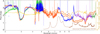 |
Fig. 11 Zoom of the benchmark model spectrum (orange) and estimated uncertainties on the calculation (light orange filled region) in the JWST spectral range, overplotted on the NIRSpec-MIRI combined spectrum. The astronomical PAHs emission from the HD 97300 disc is shown in order to delineate the regions where such features contribute to the spectrum (these emission features are not explicitly included in the model). |
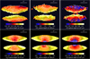 |
Fig. 12 Upper row: reproduction of Fig. 2, observed ice optical depth mapped images. Lower row: benchmark model optical depth images of the disc in H2O, CO2, and CO, as derived at 3.0, 4.26, 4.67 μm calculated against the reference continuum intensities taken at 3.7, 4.32, 4.72 μm, respectively. Over-plotted white contours show the flux intensities at the band centres, normalised to their maximum in the map. The last contour is at 5% from the maximum which is approximately the limit achieved in the observations. |
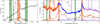 |
Fig. 13 Left panel: NIRSpec-IFU spectrum in the region covering the CH stretching mode of astronomical PAH bands. Highlighted as filled regions (orange, green) are the wavelength spans corresponding to the different spectrophotometric filters we applied for our analysis. Green filters serve as continuum references to determine the continuum to be subtracted from the orange filter, which covers the astronomical PAH feature at 3.28 μm, while excluding the adjacent Pfund δ H emission line. Right panel: MIRI-MRS spectrum in each observed channel (Ch2 red, Ch3 blue, Ch4 purple). Highlighted as filled regions (orange, green) are the wavelength spans corresponding to the different spectrophotometric filters we applied for our analysis, and corresponding to specific bands of interest in the spectrum. The orange filters are tailored to measure the main emission bands contributing to the astronomical PAH bands. The green filters are reference wavelengths to record potential contributions from the adjacent astronomical PAH-free continuum. Overplotted in brown is the Spitzer spectrum of HD 97300 which displays a similar astronomical PAH bands contribution. |
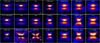 |
Fig. 14 Series of images corresponding to the integration of the observed MIRI-MRS spectra over the newly built-in filters shown in Fig. 13. Each image has been normalised to its maximum intensity in order to clearly visualize the distributions of intensities. The first row corresponds to the ‘continuum filters’ distribution. The second (middle) row contains images of the astronomical PAH bands of interest (3.29, 6.25, 7.7, 11.3 μm) and H2 (6.909, 9.667 μm) emission lines. The lowest row shows the intensity in bands of interest once subtracted by the adjacent continuum reference intensity, then also normalised to observe the intensity distributions. The upper row shows intensity distributions with globally rounded lobes, whereas each band corresponding to an astronomical PAH band shows a more or less pronounced X shape. The width and opening angle for this X shape are larger than those observed for the H2 emission lines tracing the H2 wind, the latter being more ‘nested’ within this astronomical PAH band X shape. |
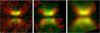 |
Fig. 15 Astronomical PAH band-H2 wind composite images. Left: composite of the 3.28 μm astronomical PAH band (in red) and the 3.235 μm H2 1–0 O(5) line (in green). Middle: composite of the 6.25 μm astronomical PAH band (in red) and the 6.909 μm H2 S(5) line (in green). Right: composite of the 11.3 μm astronomical PAH band (in red) and the 9.667 μm H2 S(3) line (in green). |
3.7.2 Simple model of a wind with astro-PAHs
We show that the observations can be explained to first order by adding a simplified astro-PAH model to the benchmark disc model with an extended atmosphere. The astro-PAHs wind contribution is described here and illustrated in the lower sketch of Fig. 5. A simple way to include such a wind consists of matter ejected from a conical structure with opening angles from the disc and whose base start from a radius rwind to rwind + δrwind. The dependence of density on the height of the wind is not easy to set, but models show it should not decrease strongly past the disc surface (Lesur 2021b; Ray & Ferreira 2021). We define
![$\rho^{\text {wind}}(\mathrm{r}, \mathrm{z})=\delta_{\text {wind}} \frac{\rho[\mathrm{r}, \mathrm{z}=\zeta \mathrm{H}(\mathrm{r})]}{[|\mathrm{z}| /[\zeta \mathrm{H}(\mathrm{r})]]^{-\gamma}} \times\left(\frac{\mathrm{r}_{\text {wind}}}{\mathrm{r}}\right)^{2};|\mathrm{z}|>\zeta \mathrm{H}(\mathrm{r}),$](/articles/aa/full_html/2025/06/aa52966-24/aa52966-24-eq8.png) (5)
(5)
where ζ is a multiplicative factor to the local scale height at which the wind begins, considered as the disc surface for the wind, and the density boundaries (ρwind = 0) are defined by rwind to rwind + δ rwind, and the θin and θout angles. These different components (settling, extended atmosphere, wind) are depicted in Fig. 5. γ defines the order of the decrease of the density with respect to the scale height. We adopt ζ = 2; that is, the wind density takes its origin at about two scale heights and evolves with γ = 1. The (rwind/r)2 factor assumes a dilution factor if the primary source of excitation comes from the stellar photons.
The astro-PAHs spectral grain model was adapted from the small PAH-Carbonaceous Grains description of Li & Draine (2001), in particular the cross-sections and profiles describing the different bands. From the extinction cross-section, we built small grain properties for the carriers constituting this wind. We do not fully treat the stochastic emission properties of such astro-PAHs, since such a treatment is out of the scope of this article. Instead, we make a simplified hypothesis to approach this. We assign the carriers a fixed emission temperature. By doing this we intrinsically assume that we deal both with the same size distribution of small astro-PAHs in the wind and that photoexcitation leads to the same internal equilibrium temperature – and thus infrared fluorescence emission cascade – irrespective of where these astronomical PAH carriers are in the wind. The emission intensity is thus modulated by the (radially and vertically decreasing) density of the carriers and the stellar photons dilution factor. The parametrisation from Eq. (5) discussed above, allows us to describe the observations, but additional studies would be needed to further constrain these astronomical PAHs. At this stage we cannot exclude thermal excitation of the carriers.
The result of the extended atmosphere model added by this astro-PAH wind, assuming θin = 49∘ and θout = 36∘, rwind = 40 au, δrwind = 25 au, ζ = 2, and an equilibrium temperature for the astro-PAHs of 600 K, is shown in Fig. 16 and the resulting model spectrum in Fig. A.4. The addition of this wind allows us to explain, to first order, the shape of the observed images in the MIR with MIRI, in and out of the astronomical PAHs wavelengths, and with an X shape, which takes on particular prominence when the aromatic bands are crossed.
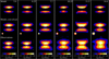 |
Fig. 16 Extension of the benchmark model to test the presence of an astro-PAH wind component. (upper) Model images at full resolution for selected wavelengths spanning the MIR for bands including astronomical PAH band contributions (6.25, 7.7, 11.3 μm) or bands representing the adjacent continuum (5.8, 10.25, 14.4 μm), for comparison. (middle) Model images once convolved with the JWST PSF. Note the alternance of a more rounded shape for continuum-dominated bands and a chalice/hourglass shape for those with astronomical PAHs contributions. (lower row) Observed MIRI images. The colorbars indicate the intensity levels, normalised to the maximum intensity for each image, on a log scale. A version of this same figure with a uniform red temperature color table is presented in the appendix. |
4 Conclusions
We have modelled the full scattering radiative transfer in the very large, almost edge-on Tau 042021 disc, including the evolution of the size and shape of icy dust grains. We added astro-PAHs as a necessary component to explain the observations covering the NIR to MIR with NIRSpec and MIRI IFUs. The essential features of the icy dust grains in the Tau 042021 disc are as follows:
The high NIR to FIR intensity ratio in the observations implies efficient scattering by grains 1–3 microns in size, and thus grains grow to at least the micron size in this disc. In agreement with previous studies, grains larger than tens of microns settle towards the disc midplane;
With such a close to edge-on disc, the observations are highly sensitive to the vertical density distribution. We have shown that reproduction of the multi-wavelength distribution of intensities in the images of Tau 042021 requires a radiative transfer model with an atmosphere extending above the classical pure isothermal vertical scale height, for scale heights >> 1, unlike in other discs such as HH30;
Deep ice absorptions are observed, indicating the presence of the major ices H2O, CO, and CO2. The spatial distribution of these ices is revealed by constructing optical depth images comparing the absorption features to the adjacent continuum. The ices are determined to be present up to high altitudes above the disc midplane; that is, above three scale heights. This suggests that ices observed in the upper atmosphere of the vertical density profile are either sufficiently well protected from VUV photons – both those external to the cloud, and the direct illumination by the source (shielded by the innermost grains) – to prevent significant desorption, or are replenished on short timescales; that is, have been relatively recently dragged or entrained into the upper atmosphere. For H2O and CO2, this vertical frontier is observationally limited only by the sensitivity of JWST, and ices may be present even higher in the disc than probed here. Apart from the very inner part of the disc, the radiative transfer is thus dominated by ice covered dust grains;
These observations underline the presence of a wind containing the carriers of astronomical PAHs. It appears as an X-shaped emission at the wavelengths of the characteristic MIR astronomical PAH bands; that is, around 3.3, 6.2, 7.7, and 11.3 microns. We provide a framework for interpreting the observations and to show that the astronomical PAH emission is more extended than the ice and dust continuum;
Images of the astronomical PAH emission and the emission of H2 in Tau 042021 seem to indicate that the spectral bands linked to astronomical PAH carriers outline a conical envelope encasing the H2 emission. This arrangement suggests that the transitions associated with these two carriers form a layered, step-like structure. This is particularly interesting in the context of the conclusion from previous studies proposing that the warm molecular layer traced by 12CO is situated between the 5–8 μm scattered light marking the disc surface and the X-shaped feature; in other words, that moving outwards perpendicular to the conical structure’s walls would reveal successive boundary layers. These layers would therefore follow a stratified pattern – consisting of an embedded wind composed of H2, astronomical PAHs, and warm 12CO – before transitioning into the extended atmosphere filled with gas and dust particles. Further studies are needed to refine the constraints on the emission characteristics and underlying physics of the astronomical PAHs in Tau 042021.
Acknowledgements
Support for program No. 1751 was provided by NASA through a grant from the Space Telescope Science Institute, which is operated by the Association of Universities for Research in Astronomy, Inc., under NASA contract NAS 5-03127. E.D. and J.A.N. acknowledge support from French Programme National ‘Physique et Chimie du Milieu Interstellaire’ (PCMI) of the CNRS/INSU with the INC/INP, co-funded by the CEA and the CNES. A portion of this research was carried out at the Jet Propulsion Laboratory, California Institute of Technology, under a contract with the National Aeronautics and Space Administration (80NM0018D0004). D.H. is supported by a Center for Informatics and Computation in Astronomy (CICA) grant and grant number 110J0353I9 from the Ministry of Education of Taiwan. D.H. also acknowledges support from the National Science and Technology Council, Taiwan (Grant NSTC111-2112-M-007-014MY3, NSTC113-2639-M-A49-002-ASP, and NSTC113-981 2112-M-007-027). M.E.P. acknowledges support by INAF grant within the program Ricerca Fondamentale 2022. This work is based in part on observations made with the NASA/ESA/CSA James Webb Space Telescope. The data were obtained from the Mikulski Archive for Space Telescopes at the Space Telescope Science Institute, which is operated by the Association of Universities for Research in Astronomy, Inc., under NASA contract NAS 5-03127 for JWST. These observations are associated with program No. 1751 – Mapping inclined disk astrochemical signatures (MIDAS). The data described here may be obtained from https://dx.doi.org/10.17909/q1ec-wj71.
Appendix A Images with a uniform color table and model spectrum including the astro-PAHs grain model
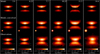 |
Fig. A.3 Benchmark model including an astro-PAHs wind component as in Fig. 16 coded with a single red temperature color table. (upper) Model images at full resolution for selected wavelengths spanning the MIR for bands including astro-PAHs contributions (6.25, 7.7, 11.3 μm) or bands representing adjacent bands with more continuum (5.8, 10.25, 14.4 μm) for comparison. (middle) Model images once convolved with JWST PSF. Note the alternance of more rounded shape for continuum dominated bands and chalice/hourglass shape for the one with astro-PAHs contribution. (lower row) observed MIRI images. The colorbars indicate the intensity levels, normalised to the maximum intensity for each image, in log scale. |
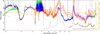 |
Fig. A.4 Zoom of the benchmark model spectrum including the astro-PAHs grain model (orange) and estimated uncertainties on the calculation (light orange filled region) in the JWST spectral range, overplotted on the NIRSpec-MIRI combined spectrum. Note the emission in the model is higher in the 8–10 microns, which may be related to an overestimate of the silicates stretching mode contribution in emission in this range. The astronomical PAHs emission from the HD97300 disc is also shown in order to delineate the astronomical PAHs spectral profiles observed in another disc. |
References
- Aikawa, Y., Kamuro, D., Sakon, I., et al. 2012, A&A, 538, A57 [NASA ADS] [CrossRef] [EDP Sciences] [Google Scholar]
- Allamandola, L. J., Tielens, A. G. G. M., & Barker, J. R., 1985, ApJ, 290, L25 [Google Scholar]
- Argyriou, I., Glasse, A., Law, D. R., et al. 2023, A&A, 675, A111 [NASA ADS] [CrossRef] [EDP Sciences] [Google Scholar]
- Armitage, P. J., 2019, Physical Processes in Protoplanetary Disks, eds. M. Audard, M. R. Meyer, & Y. Alibert (Berlin, Heidelberg: Springer Berlin Heidelberg), 1 [Google Scholar]
- Arulanantham, N., McClure, M., Pontoppidan, K., et al. 2024, ApJ, 965, L13 [NASA ADS] [CrossRef] [Google Scholar]
- Bergner, J. B., Sturm, J. A., Piacentino, E. L., et al. 2024, ApJ, 975, 166 [NASA ADS] [CrossRef] [Google Scholar]
- Burrows, C. J., Stapelfeldt, K. R., Watson, A. M., et al. 1996, ApJ, 473, 437 [Google Scholar]
- Chiang, E., & Goldreich, P., 1997, ApJ, 490, 368 [NASA ADS] [CrossRef] [Google Scholar]
- Chown, R., Sidhu, A., Peeters, E., et al. 2024, A&A, 685, A75 [NASA ADS] [CrossRef] [EDP Sciences] [Google Scholar]
- Ciesla, F. J., 2010, ApJ, 723, 514 [NASA ADS] [CrossRef] [Google Scholar]
- Cutri, R. M., Skrutskie, M. F., van Dyk, S., et al. 2003, The IRSA 2MASS All-Sky Point Source Catalog, NASA/IPAC Infrared Science Archive, http://irsa.ipac.caltech.edu/applications/Gator/ [Google Scholar]
- Dartois, E., 2006, A&A, 445, 959 [NASA ADS] [CrossRef] [EDP Sciences] [Google Scholar]
- Dartois, E., Noble, J. A., Ysard, N., Demyk, K., & Chabot, M., 2022, A&A, 666, A153 [NASA ADS] [CrossRef] [EDP Sciences] [Google Scholar]
- Dartois, E., Noble, J. A., Caselli, P., et al. 2024, Nat. Astron., 8, 359 [NASA ADS] [CrossRef] [Google Scholar]
- Dominik, C., Min, M., & Tazaki, R., 2021, Astrophysics Source Code Library [record ascl:2104.010] [Google Scholar]
- Draine, B. T., & Flatau, P. J., 2013, arXiv e-prints [arXiv:1305.6497] [Google Scholar]
- Duchêne, G., Stapelfeldt, K., Isella, A., et al. 2014, in Exploring the Formation and Evolution of Planetary Systems, 299, eds. M. Booth, B. C. Matthews, & J. R. Graham, 111 [Google Scholar]
- Duchêne, G., Ménard, F., Stapelfeldt, K. R., et al. 2024, AJ, 167, 77 [CrossRef] [Google Scholar]
- Dullemond, C. P., Juhasz, A., Pohl, A., et al. 2012, Astrophysics Source Code Library [record ascl:1202.015] [Google Scholar]
- Dutrey, A., Wakelam, V., Boehler, Y., et al. 2011, A&A, 535, A104 [NASA ADS] [CrossRef] [EDP Sciences] [Google Scholar]
- Dutrey, A., Guilloteau, S., Piétu, V., et al. 2017, A&A, 607, A130 [CrossRef] [EDP Sciences] [Google Scholar]
- Federman, S. A., Megeath, S. T., Rubinstein, A. E., et al. 2024, ApJ, 966, 41 [CrossRef] [Google Scholar]
- Galli, P. A. B., Loinard, L., Bouy, H., et al. 2019, A&A, 630, A137 [NASA ADS] [CrossRef] [EDP Sciences] [Google Scholar]
- Guilloteau, S., Piétu, V., Chapillon, E., et al. 2016, A&A, 586, L1 [NASA ADS] [CrossRef] [EDP Sciences] [Google Scholar]
- Hirose, S., & Turner, N. J., 2011, ApJ, 732, L30 [NASA ADS] [CrossRef] [Google Scholar]
- Kama, M., Min, M., & Dominik, C., 2009, A&A, 506, 1199 [NASA ADS] [CrossRef] [EDP Sciences] [Google Scholar]
- Kenyon, S. J., Dobrzycka, D., & Hartmann, L., 1994, AJ, 108, 1872 [NASA ADS] [CrossRef] [Google Scholar]
- Law, D. D., Morrison, J. E., Argyriou, I., et al. 2023, AJ, 166, 45 [NASA ADS] [CrossRef] [Google Scholar]
- Lebreuilly, U., Commerçon, B., & Laibe, G., 2019, A&A, 626, A96 [NASA ADS] [CrossRef] [EDP Sciences] [Google Scholar]
- Lebreuilly, U., Vallucci-Goy, V., Guillet, V., Lombart, M., & Marchand, P., 2023, MNRAS, 518, 3326 [Google Scholar]
- Lee, Y.-N., Ray, B., Marchand, P., & Hennebelle, P., 2024, ApJ, 961, L28 [NASA ADS] [CrossRef] [Google Scholar]
- Leger, A., & Puget, J. L., 1984, A&A, 137, L5 [Google Scholar]
- Le Gouellec, V. J. M., Lew, B. W. P., Greene, T. P., et al. 2024, ApJ, submitted [arXiv:2410.11095] [Google Scholar]
- Lesur, G. R., 2021a, J. Plasma Phys., 87, 205870101 [Google Scholar]
- Lesur, G. R. J. 2021b, A&A, 650, A35 [NASA ADS] [CrossRef] [EDP Sciences] [Google Scholar]
- Li, A., & Draine, B. T., 2001, ApJ, 554, 778 [Google Scholar]
- Luhman, K. L., Mamajek, E. E., Allen, P. R., & Cruz, K. L., 2009, ApJ, 703, 399 [NASA ADS] [CrossRef] [Google Scholar]
- Lynden-Bell, D., & Pringle, J. E., 1974, MNRAS, 168, 603 [Google Scholar]
- Marchand, P., Guillet, V., Lebreuilly, U., & Mac Low, M. M., 2022, A&A, 666, A27 [NASA ADS] [CrossRef] [EDP Sciences] [Google Scholar]
- Marchand, P., Lebreuilly, U., Mac Low, M. M., & Guillet, V., 2023, A&A, 670, A61 [NASA ADS] [CrossRef] [EDP Sciences] [Google Scholar]
- Mathis, J. S., Rumpl, W., & Nordsieck, K. H., 1977, ApJ, 217, 425 [Google Scholar]
- McClure, M. K., Rocha, W. R. M., Pontoppidan, K. M., et al. 2023, Nat. Astron., 7, 431 [NASA ADS] [CrossRef] [Google Scholar]
- Min, M., Hovenier, J. W., & de Koter, A., 2005, A&A, 432, 909 [NASA ADS] [CrossRef] [EDP Sciences] [Google Scholar]
- Montesinos, M., Cuello, N., Olofsson, J., et al. 2021, ApJ, 910, 31 [CrossRef] [Google Scholar]
- Ormel, C. W., 2014, ApJ, 789, L18 [Google Scholar]
- Paruta, P., Hendrix, T., & Keppens, R., 2016, Astron. Comput., 16, 155 [NASA ADS] [CrossRef] [Google Scholar]
- Pascucci, I., Beck, T. L., Cabrit, S., et al. 2025, Nat. Astron., 9, 81 [Google Scholar]
- Peeters, E., Hony, S., Van Kerckhoven, C., et al. 2002, A&A, 390, 1089 [NASA ADS] [CrossRef] [EDP Sciences] [Google Scholar]
- Ray, T. P., & Ferreira, J., 2021, New A Rev., 93, 101615 [NASA ADS] [CrossRef] [Google Scholar]
- Rebull, L. M., Padgett, D. L., McCabe, C. E., et al. 2010, ApJS, 186, 259 [NASA ADS] [CrossRef] [Google Scholar]
- Rieke, M. J., Kelly, D. M., Misselt, K., et al. 2023, PASP, 135, 028001 [CrossRef] [Google Scholar]
- Roccatagliata, V., Franciosini, E., Sacco, G. G., Randich, S., & Sicilia-Aguilar, A., 2020, A&A, 638, A85 [NASA ADS] [CrossRef] [EDP Sciences] [Google Scholar]
- Salyk, C., Blake, G. A., Boogert, A. C. A., & Brown, J. M., 2011, ApJ, 743, 112 [NASA ADS] [CrossRef] [Google Scholar]
- Silsbee, K., Ivlev, A. V., Sipilä, O., Caselli, P., & Zhao, B., 2020, A&A, 641, A39 [NASA ADS] [CrossRef] [EDP Sciences] [Google Scholar]
- Stapelfeldt, K. R., Duchêne, G., Perrin, M., et al. 2014, in Exploring the Formation and Evolution of Planetary Systems, 299, eds. M. Booth, B. C. Matthews, & J. R. Graham, 99 [Google Scholar]
- Sturm, J. A., McClure, M. K., Beck, T. L., et al. 2023a, A&A, 679, A138 [NASA ADS] [CrossRef] [EDP Sciences] [Google Scholar]
- Sturm, J. A., McClure, M. K., Bergner, J. B., et al. 2023b, A&A, 677, A18 [NASA ADS] [CrossRef] [EDP Sciences] [Google Scholar]
- Sturm, J. A., McClure, M. K., Law, C. J., et al. 2023c, A&A, 677, A17 [NASA ADS] [CrossRef] [EDP Sciences] [Google Scholar]
- Sturm, J. A., McClure, M. K., Harsono, D., et al. 2024, A&A, 689, A92 [NASA ADS] [CrossRef] [EDP Sciences] [Google Scholar]
- Tazaki, R., Ménard, F., Duchêne, G., et al. 2025, ApJ, 980, 49 [Google Scholar]
- van Diedenhoven, B., Peeters, E., Van Kerckhoven, C., et al. 2004, ApJ, 611, 928 [NASA ADS] [CrossRef] [Google Scholar]
- Villenave, M., Ménard, F., Dent, W. R. F., et al. 2020, A&A, 642, A164 [EDP Sciences] [Google Scholar]
- Villenave, M., Podio, L., Duchêne, G., et al. 2023, ApJ, 946, 70 [NASA ADS] [CrossRef] [Google Scholar]
- Weingartner, J. C., & Draine, B. T., 2001, ApJ, 548, 296 [Google Scholar]
- Yang, Y.-L., Green, J. D., Pontoppidan, K. M., et al. 2022, ApJ, 941, L13 [NASA ADS] [CrossRef] [Google Scholar]
All Figures
|
Fig. 1 NIRSpec observations of Tau 042021. Left: illustrative photometric image at 3.7 μm, showing the overall structure of the disc in continuum emission flux. Right: NIRSpec spectra of Tau 042021. The total flux integrated over both lobes is shown in black. The individual contributions of the upper emission lobe (red) and lower lobe (blue) are shown. The upper-to-lower lobe flux ratio is shown in gold. The ratio generally lies at around 2 across the continuum, whereas in some parts of the profile of the absorption bands, the lower lobe is more extinct than the upper. Some gaps in the spectra are due to the corresponding ‘gaps’ in the NIRSpec observations at some wavelengths. The photometry from NIRCam images presented in Duchêne et al. (2024) are shown in orange (the corresponding filter shapes for the NIRCam filters F200W and F444W are shown below in black). The corresponding photometry obtained by integrating the spectra over the same filter profiles from our work are shown in green. |
| In the text | |
|
Fig. 2 Observed H2O, CO2, and CO ice optical depth mapped images of the disc at 3.0, 4.26, and 4.67 μm derived from the NIRSpec image at those wavelengths calculated relative to the reference continuum intensities taken at 3.7, 4.32, and 4.72 μm, respectively. Over-plotted white contours show the flux intensity at the band centres, normalised to their maximum in the map. The last contour is at 5% from the maximum. |
| In the text | |
|
Fig. 3 Band profiles comparison. The integrated NIRSpec spectrum from the north lobe of Tau 042021, in a sub-region unaffected by NIRSpec IFU masking to fully sample the profile, is shown in red (multiplied by 1.2). It is compared to a typical dense cloud spectrum (NIRCam + NIRSpec IFU, black, flux (multiplied by two) observed at high extinction in Chamaeleon I (McClure et al. 2023). Note the inversion in the shape for the CO2 ice band profile around 4.27 μm betraying differences in radiative transfer properties. A laboratory transmittance spectrum (blue) of a H2O:CO2 ice film mixture used in the optical constants determination in Dartois et al. (2024) has been converted to flux scale for comparison. Spectra have been scaled to have similar optical depths in the ice absorption features in order to compare their profiles. |
| In the text | |
|
Fig. 4 Comparison of a combined NIRSpec (black) and MIRI (each channel is represented with a distinct colour: orange, blue, purple, or green) spectrum of Tau 042021 with spectra representing gas-phase contributions from CO gas (dark blue) and astronomical PAHs (brown) to the spectrum. See text for details. |
| In the text | |
|
Fig. 5 Schematic edge-on views of the protoplanetary disc models used in this article. Upper panel: The ‘standard’ model includes a main disc flaring component with grains of sizes smaller than a critical size asettling and, possibly, settled dust grains for sizes above this size limit. The internal part of the disc (below rcav) can harbour a partially filled cavity (where the density is multiplied by a δcav < 1 factor). See Sect. 3.5 for details of the other parameters used in the ‘standard model’. Central panel: The extended atmosphere model, or ‘benchmark’ model, detailed in Sect. 3.6, supersedes the ‘standard’ model, while still including its main disc flaring component and settled dust grains. This model comprises an extended tenuous dust atmosphere lying above the classical purely hydrostatic model. Lower panel: The ‘wind’ model, detailed in Sect. 3.7.2, includes all the components from the benchmark model with the addition of a wind whose main parametrisation is shown here. Angles are given from the midplane axis. |
| In the text | |
|
Fig. 6 Standard model. (upper) Model images at full resolution for selected wavelengths spanning the NIR to millimetre range. (middle) Model images once convolved with the JWST or ALMA PSF. (lower) JWST NIRSpec (2.2 and 3.7 μm), MIRI (7.7 and 14.4 μm), and ALMA Band 7 (890 μm) observations. Blue ticks are guides to the small wings observed at about 22.5∘, especially in the NIR, whereas brown tickmarks indicate an angle of 36∘ overplotted on the 7.7 μm image, corresponding to the angle for the X-shape discussed by Duchêne et al. (2024), and close to the H2 wind (semi-opening) angle previously observed in the 35–38.5∘ range by Arulanantham et al. (2024); Pascucci et al. (2025). The colorbars indicate the intensity levels, normalised to the maximum intensity for each image, in log scale except for ALMA data presented in linear scale. The right panel are cuts along the vertical line through the centre of the disc observations and models at the corresponding wavelengths (2.2 μm−blue; 3.7 μm-orange; 7.7 μm – purple; 14.4 μm – green, and 890 μm – brown). The spatial scale is expanded (shown with the black arrows) by a factor of two as compared to the images for a clearer view. The adopted blue-red-yellow color table was chosen to enhance the visibility of details in the structure. A version of this same figure with a uniform red temperature color table is presented in the appendix. |
| In the text | |
|
Fig. 7 Vertical density profile for a scale height of H0 = 10, normalised to the midplane density, considering an isothermal model (solid line) and including an extended atmosphere as shown in Eq. (4) for ϵ = 2.5 (dotted line) and 4 (dashed line), corresponding to an atmosphere contributing above about 3–4 × z/h. The integral of the mass increase above 3 scale heights represents about 1 × 10⁻² of the total mass for ϵ = 2.5 and about 2 × 10⁻³ of the total mass for ϵ = 4, but strongly affects the radiative transfer in the upper layers. |
| In the text | |
|
Fig. 8 Selected NIR-to-FIR characteristic intensity ratios. Left: intensity ratios calculated as a function of asetting for the benchmark model. amin, defining the evolution of the small and large dust grain distributions, is varied from the MRN value (0.005 μm) to 3 μm. The shaded regions delimited by dotted lines represent the expected observed intensity ratios, taking into account the variations between JWST observations and previous photometric data points. The central panels are 2D representations of the same model results. Right: exploration of the effect of cavity radius on the 21 to 890 μm intensity ratio in the benchmark model, which includes the presence of an inner, partially filled, cavity. A better agreement is obtained for rcav above several tens of astronomical units. |
| In the text | |
|
Fig. 9 Benchmark model, i.e. the ‘standard’ disc model plus an extended atmosphere. The nomenclature is the same as for Fig. 6. The presence of an efficient scatterer rather high up in the disc in this extended atmosphere allows for a better reproduction of the vertical distribution of observed intensities. See text for details. A version of this same figure with a uniform red temperature colour table is presented in the appendix. |
| In the text | |
|
Fig. 10 Benchmark model spectrum (orange) overplotted on the SED data for Tau 042021, normalised to the observed average flux in the NIRSpec range. Blue photometric points are taken from Table 4 of Duchêne et al. (2024). Orange symbols correspond to the ≤ 2.2 μm photometric points adjusted by a factor to match the JWST flux, taking into account the known potential variability of the source (see text for details). Error bars (3σ) are given for the long wavelength photometric points from Spitzer/MIPS, Herschel/PACS and Herschel/SPIRE, retrieved from published point source catalogues. |
| In the text | |
|
Fig. 11 Zoom of the benchmark model spectrum (orange) and estimated uncertainties on the calculation (light orange filled region) in the JWST spectral range, overplotted on the NIRSpec-MIRI combined spectrum. The astronomical PAHs emission from the HD 97300 disc is shown in order to delineate the regions where such features contribute to the spectrum (these emission features are not explicitly included in the model). |
| In the text | |
|
Fig. 12 Upper row: reproduction of Fig. 2, observed ice optical depth mapped images. Lower row: benchmark model optical depth images of the disc in H2O, CO2, and CO, as derived at 3.0, 4.26, 4.67 μm calculated against the reference continuum intensities taken at 3.7, 4.32, 4.72 μm, respectively. Over-plotted white contours show the flux intensities at the band centres, normalised to their maximum in the map. The last contour is at 5% from the maximum which is approximately the limit achieved in the observations. |
| In the text | |
|
Fig. 13 Left panel: NIRSpec-IFU spectrum in the region covering the CH stretching mode of astronomical PAH bands. Highlighted as filled regions (orange, green) are the wavelength spans corresponding to the different spectrophotometric filters we applied for our analysis. Green filters serve as continuum references to determine the continuum to be subtracted from the orange filter, which covers the astronomical PAH feature at 3.28 μm, while excluding the adjacent Pfund δ H emission line. Right panel: MIRI-MRS spectrum in each observed channel (Ch2 red, Ch3 blue, Ch4 purple). Highlighted as filled regions (orange, green) are the wavelength spans corresponding to the different spectrophotometric filters we applied for our analysis, and corresponding to specific bands of interest in the spectrum. The orange filters are tailored to measure the main emission bands contributing to the astronomical PAH bands. The green filters are reference wavelengths to record potential contributions from the adjacent astronomical PAH-free continuum. Overplotted in brown is the Spitzer spectrum of HD 97300 which displays a similar astronomical PAH bands contribution. |
| In the text | |
|
Fig. 14 Series of images corresponding to the integration of the observed MIRI-MRS spectra over the newly built-in filters shown in Fig. 13. Each image has been normalised to its maximum intensity in order to clearly visualize the distributions of intensities. The first row corresponds to the ‘continuum filters’ distribution. The second (middle) row contains images of the astronomical PAH bands of interest (3.29, 6.25, 7.7, 11.3 μm) and H2 (6.909, 9.667 μm) emission lines. The lowest row shows the intensity in bands of interest once subtracted by the adjacent continuum reference intensity, then also normalised to observe the intensity distributions. The upper row shows intensity distributions with globally rounded lobes, whereas each band corresponding to an astronomical PAH band shows a more or less pronounced X shape. The width and opening angle for this X shape are larger than those observed for the H2 emission lines tracing the H2 wind, the latter being more ‘nested’ within this astronomical PAH band X shape. |
| In the text | |
|
Fig. 15 Astronomical PAH band-H2 wind composite images. Left: composite of the 3.28 μm astronomical PAH band (in red) and the 3.235 μm H2 1–0 O(5) line (in green). Middle: composite of the 6.25 μm astronomical PAH band (in red) and the 6.909 μm H2 S(5) line (in green). Right: composite of the 11.3 μm astronomical PAH band (in red) and the 9.667 μm H2 S(3) line (in green). |
| In the text | |
|
Fig. 16 Extension of the benchmark model to test the presence of an astro-PAH wind component. (upper) Model images at full resolution for selected wavelengths spanning the MIR for bands including astronomical PAH band contributions (6.25, 7.7, 11.3 μm) or bands representing the adjacent continuum (5.8, 10.25, 14.4 μm), for comparison. (middle) Model images once convolved with the JWST PSF. Note the alternance of a more rounded shape for continuum-dominated bands and a chalice/hourglass shape for those with astronomical PAHs contributions. (lower row) Observed MIRI images. The colorbars indicate the intensity levels, normalised to the maximum intensity for each image, on a log scale. A version of this same figure with a uniform red temperature color table is presented in the appendix. |
| In the text | |
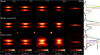 |
Fig. A.1 Standard model as in Fig. 6 coded with a single red temperature color table. |
| In the text | |
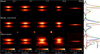 |
Fig. A.2 Benchmark model as in Fig. 9 coded with a single red temperature color table. |
| In the text | |
|
Fig. A.3 Benchmark model including an astro-PAHs wind component as in Fig. 16 coded with a single red temperature color table. (upper) Model images at full resolution for selected wavelengths spanning the MIR for bands including astro-PAHs contributions (6.25, 7.7, 11.3 μm) or bands representing adjacent bands with more continuum (5.8, 10.25, 14.4 μm) for comparison. (middle) Model images once convolved with JWST PSF. Note the alternance of more rounded shape for continuum dominated bands and chalice/hourglass shape for the one with astro-PAHs contribution. (lower row) observed MIRI images. The colorbars indicate the intensity levels, normalised to the maximum intensity for each image, in log scale. |
| In the text | |
|
Fig. A.4 Zoom of the benchmark model spectrum including the astro-PAHs grain model (orange) and estimated uncertainties on the calculation (light orange filled region) in the JWST spectral range, overplotted on the NIRSpec-MIRI combined spectrum. Note the emission in the model is higher in the 8–10 microns, which may be related to an overestimate of the silicates stretching mode contribution in emission in this range. The astronomical PAHs emission from the HD97300 disc is also shown in order to delineate the astronomical PAHs spectral profiles observed in another disc. |
| In the text | |
Current usage metrics show cumulative count of Article Views (full-text article views including HTML views, PDF and ePub downloads, according to the available data) and Abstracts Views on Vision4Press platform.
Data correspond to usage on the plateform after 2015. The current usage metrics is available 48-96 hours after online publication and is updated daily on week days.
Initial download of the metrics may take a while.