| Issue |
A&A
Volume 666, October 2022
|
|
|---|---|---|
| Article Number | A74 | |
| Number of page(s) | 19 | |
| Section | Interstellar and circumstellar matter | |
| DOI | https://doi.org/10.1051/0004-6361/202244026 | |
| Published online | 11 October 2022 | |
Synthetic Next Generation Very Large Array line observations of a massive star-forming cloud
1
Department of Physics,
PO Box 64,
00014,
University of Helsinki,
Helsinki, Finland
e-mail: This email address is being protected from spambots. You need JavaScript enabled to view it.
2
Shanghai Astronomical Observatory, Chinese Academy of Sciences,
80 Nandan Road,
Shanghai
200030, PR China
3
Department of Astronomy, Eötvös Loránd University,
Pázmány Péter sétány 1/A,
1117
Budapest, Hungary
Received:
15
May
2022
Accepted:
1
August
2022
Abstract
Context. Studies of the interstellar medium and the pre-stellar cloud evolution require spectral line observations that have a high sensitivity and high angular and velocity resolution. Regions of high-mass star formation are particularly challenging because of line-of-sight confusion, inhomogeneous physical conditions, and potentially very high optical depths.
Aims. We wish to quantify to what accuracy the physical conditions within a massive star-forming cloud can be determined from observations. We are particularly interested in the possibilities offered by the Next Generation Very Large Array (ngVLA) interferometer.
Methods. We used data from a magnetohydrodynamic simulation of star formation in a high-density environment. We concentrated on the study of a filamentary structure that has physical properties similar to a small infrared-dark cloud. We produced synthetic observations for spectral lines observable with the ngVLA and analysed these to measure column density, gas temperature, and kinematics. Results were compared to ideal line observations and the actual 3D model.
Results. For a nominal cloud distance of 4kpc, ngVLA provides a resolution of ~0.01 pc even in its most compact configuration. For abundant molecules, such as HCO+, NH3, N2H+, and CO isotopomers, cloud kinematics and structure can be mapped down to subarcsecond scales in just a few hours. For NH3, a reliable column density map could be obtained for the entire 15″ × 40″ cloud, even without the help of additional single-dish data, and kinetic temperatures are recovered to a precision of ~1 K. At higher frequencies, the loss of large-scale emission becomes noticeable. The line observations are seen to accurately trace the cloud kinematics, except for the largest scales, where some artefacts appear due to the filtering of low spatial frequencies. The line-of-sight confusion complicates the interpretation of the kinematics, and the usefulness of collapse indicators based on the expected blue asymmetry of optically thick lines is limited.
Conclusions. The ngVLA will be able to provide accurate data on the small-scale structure and the physical and chemical state of star-forming clouds, even in high-mass star-forming regions at kiloparsec distances. Complementary single-dish data are still essential for estimates of the total column density and the large-scale kinematics.
Key words: ISM: clouds / ISM: molecules / radio lines: ISM / stars: formation / stars: protostars
© M. Juvela et al. 2022
 Open Access article, published by EDP Sciences, under the terms of the Creative Commons Attribution License (https://creativecommons.org/licenses/by/4.0), which permits unrestricted use, distribution, and reproduction in any medium, provided the original work is properly cited.
This article is published in open access under the Subscribe-to-Open model. This email address is being protected from spambots. You need JavaScript enabled to view it. to support open access publication.
1 Introduction
Progress in star-formation (SF) studies is made via a combination of observations and numerical simulations. Many open questions remain regarding the cloud formation, the balance between gravity, turbulence, and magnetic fields at different scales, how filamentary structures are formed, how they fragment, and how mass accretion takes place at different scales, from clouds to filaments and finally to protostellar cores – and how all these processes differ between star-forming regions (Motte et al. 2018; Hacar et al. 2022; Pattle et al. 2022). We also need a better understanding of the interstellar medium (ISM) itself, the gas, and the dust, which are used as tracers of the SF process and affect, and are affected by, the SF.
Understanding high-mass SF is particularly important as massive stars are crucial to many astrophysical processes, and their ionising radiation and stellar winds, as well as the heavy elements produced by supernovae, affect their host galaxies (Kennicutt 2005). Massive stars are formed partly in infrared-dark clouds (IRDCs), which are massive (M ≳ 1000 M⊙), cold (on average T ~ 10–20K), and dense (Σ ~ 0.02 g cm−2; Peretto et al. 2010; Kainulainen & Tan 2013; Tan et al. 2014; Lim et al. 2016).
Studies suggest that high-mass star-forming cores fragment as soon as they lose turbulent and magnetic support (Csengeri et al. 2011), and numerical simulations show clouds not to be in equilibrium (Padoan et al. 2001; Vázquez-Semadeni et al. 2007). Although simulations provide a direct handle on the dependences between SF and the environment where SF takes place, different views exist regarding the main causes of the high-mass SF (Zinnecker & Yorke 2007; Tan 2018; Motte et al. 2018). It is still not clear whether high-mass stars form through competitive accretion (Larson 1992; Bonnell et al. 2001, 2004) or core-accretion (Larson 1981; McKee 1999; McKee & Tan 2003) or via large-scale processes that are driven mainly either by gravity (Vázquez-Semadeni et al. 2019; Naranjo-Romero et al. 2022) or turbulent inertial flows (Padoan et al. 2020; Pelkonen et al. 2021) – or rather the relative importance of the different mechanisms is in different physical environments.
The SF theories are all supported by numerical simulations, although with some differences in the assumed boundary conditions and included physics. It is essential that these paradigms be tested against real observations in an objective way. Observations can be used to estimate physical parameters (column densities, volume densities, and temperatures) and the kinematics and chemistry in different phases of the SF process, and to quantify the resulting populations of clumps, filaments, and cores. These can all be compared to the model predictions, using synthetic observations that take into account, at least partially, the complexity of the source structure and the variations in the physical conditions along the line of sight (LOS) and inside the finite telescope beam.
To accurately test SF theories, one needs observations that cover large areas with high sensitivity and fidelity and, on the other hand, have the resolution to probe the small-scale core fragmentation and the initial stages of protostellar collapse. Recent continuum observations, for example the surveys conducted with the Herschel Space Observatory (Pilbratt et al. 2010), have resulted in significant advances in the understanding of the structure of the star-forming clouds and the large-scale context of SF. However, spectral line observations remain crucial, to mitigate the effects of LOS confusion and to gain direct access to the physical properties, kinematics, and chemistry of the gas component.
Radio interferometers are essential for studies of the small structures, the cloud cores with sizes below ~0.1 pc or even the core fragmentation down to ~1000 au scales (Tokuda et al. 2020; Sahu et al. 2021). Interferometry is also needed for the more distant targets, including the typical high-mass star-forming clouds that are at kiloparsec distances (Liu et al. 2020; Beuther et al. 2021; O’Neill et al. 2021; Motte et al. 2022). Instruments such as the Atacama Large Millimeter/submillimeter Array (ALMA1), the Submillimetre Array (SMA2), and the IRAM NOrthern Extended Millimeter Array (NOEMA3) already provide subarcsecond resolution.
The Next Generation Very Large Array (ngVLA4) is the planned extension of the Karl G. Jansky Very Large Array (VLA5). It will cover frequencies 1.2–116 GHz with (at the highest frequencies) a maximum instantaneous bandwidth of 20 GHz and with a sensitivity and angular resolution potentially exceeding those of both the current VLA and ALMA instruments. The ngVLA will also complement the radio-frequency coverage of ALMA and SKA6 that, respectively, operate mainly at higher and lower frequencies. It will be complementary also by providing high-resolution observations of the northern sky. The ngVLA will be able to observe basic transitions of several key molecules, such as NH3, some of which are not accessible to ALMA but are important for SF studies and especially for the study of the cold ISM and the early phases of the SF process.
In this paper we study, as a test case, synthetic observations of a massive filamentary cloud. The target has properties similar to an IRDC capable of giving birth to high-mass stars. The cloud model is obtained from a magnetohydrodynamic (MHD) simulation, which is post-processed with radiative transfer calculations to predict line emission in several transitions that are accessible to the ngVLA. The simulated line data are processed with the CASA program7 to make predictions for actual ngVLA observations, including realistic noise and effects of the interferometric mode of observations. This is part of an ngVLA community study, where we investigate the use of the ngVLA interferometer for observations of star-forming clouds. In the present paper, the emphasis is on moderately extended structures, and we concentrate on observations with the most compact ngVLA antenna configuration. Smaller scales (e.g. sub-fragmentation of cores) will be addressed in future publications.
The contents of the paper are the following. Section 2 describes the MHD runs (Sect. 2.1), radiative transfer modelling (Sect. 2.2), and CASA simulations (Sect. 2.3). The synthetic observations are analysed in Sect. 3, regarding column densities (Sect. 3.2) and temperatures (Sect. 3.3) and cloud kinematics (3.4). We discuss the results in Sect. 4 before listing the final conclusions in Sect. 5.
2 Simulated Observations
2.1 MHD Simulations
As a starting point for the synthetic observations, we used the density and velocity fields from the MHD simulation described in Haugbølle et al. (2018). The MHD run covers a volume of (4 pc)3, using octree spatial discretisation with a root grid of 2563 cells and up to five levels of refinement, reaching a best linear resolution of 100 au (4.88 × 10⁻⁴ pc). The refinement was based on density, especially to resolve the collapsing cores. Sink particles were used to represent collapsed regions where the density exceeded the average density by a factor of 105–106 and where stars are thus forming. The total mass contained in the (4 pc)3 box is about 3000 M⊙. In the snapshot used in this paper, over 400 stars have already formed, and these were also used in the subsequent radiative transfer modelling as radiation sources. Details of the MHD simulation and a study of formed stellar populations can be found in Haugbølle et al. (2018).
2.2 Radiative Transfer Modelling
We concentrated on the densest part of the model and extracted a (1.84pc)3 sub-volume out of the full (4pc)3 MHD run. The sub-volume contains 230 young stars with masses ranging from sub-solar to 36 M⊙ and includes two main density enhancement that, in the selected view direction “x”, appear as a single elongated structure (Fig. 1a). We refer to this structure as “the filament”. In 3D, it consists of a northern and a southern clumps, which are connected also in 3D, but only by narrow bridges that are inclined by about 45° with respect to the observer LOS (Fig. 1b). The 3D nature of the object is therefore different from its appearance in the projected images. Figure 2 shows the mass surface density towards the direction x. The figure also shows the outlines of the northern and southern clumps, which are in 3D defined by density isosurfaces.
We started by modelling the dust component, using the dust properties from Weingartner & Draine (2001), the Case B that has a selective extinction of RV = 5.5, the high value being appropriate for dense clouds. The calculations were carried out with the radiative transfer programme SOC (Juvela 2019), using the full octree discretisation of the MHD model. The dust heating included an isotropic external field (Mathis et al. 1983) and the contribution of the embedded stars, which were modelled as as blackbody point sources, with the given luminosities and effective temperatures (Haugbølle et al. 2018). The radiative transfer calculations solved the dust temperature Tdust for each model cell, assuming that the grains are at equilibrium with the radiation field. The dust-temperature distribution has its mode at 14.3 K and extends below 10 K in dense, nonprotostellar cores. The temperature structure is not fully resolved in the immediate vicinity of stars, but temperatures at and above 100K are reached in nearly 0.1% of the cells. Because the spatial grid is highly refined close to the star-forming cores, this corresponds to a much smaller fraction of the cloud volume. The analysis of the synthetic observations of dust emission (and polarisation as a proxy of the magnetic fields) are deferred to a future publication. In this paper, only the information of the estimated large-grain dust temperatures is used. Appendix A shows a colour-temperature map, how the dust temperature distribution would appear based on 160–500 µm continuum observations.
The line modelling is based on the density and velocity fields of the MHD simulation and the results of the dust modelling, assuming that the dust temperature serves as a proxy for the gas kinetic temperature, Tkin ≈ Tdust. The line modelling was carried out with the radiative transfer program LOC (Juvela 2020), with the molecular data obtained from the LAMDA database (Schöier et al. 2005). The calculations solve the non-LTE excitation of the molecules in each cell and provide spectral line maps towards chosen directions. Spectra were computed for 13CO(1−0), C18O(1−0), HCO+(1−0), H13CO+(1−0), N2H+(1−0), NH3(1, 1), and NH3(2, 2) lines. In the case of N2H+(1−0) and NH3(1, 1), the hyperfine structure was taken into account by assuming LTE conditions between the hyperfine components (Keto 1990).
The assumed peak fractional abundances are 2 × 10⁻⁶ for 13CO, 3 × 10⁻⁷ for C18O, 5 × 10⁻¹⁰ for HCO+, 1 × 10⁻¹¹ for H13CO+, 3 × 10⁻⁸ for NH3, and 1 × 10⁻⁹ for N2H+. The abundances were further scaled with an additional density dependence n(H2)2.45/(3.0 × 108 + n(H2)2.45) (cf. Glover et al. 2010). This decreases the abundances at densities below n(H2) = 104 cm−3, reduces them by a factor of ten at n(H2) = 103 cm−3 and makes them negligible at the lowest densities, where the gas can be assumed to be mostly atomic. We did not model the depletion that could decrease the abundances at the highest densities, especially within the pre-stellar cores.
The assumption Tkin ≈ Tdust is accurate at densities close to and above 105 cm−3, where the gas–dust collisions bring the gas kinetic temperature to within a few degrees of the dust temperature (Goldsmith 2001; Young et al. 2004; Juvela & Ysard 2011). For example for N2H+(1−0), most emission comes from such high-density gas, because the critical density of the transition is close to n(H2) = 105 cm−3. There is a range of densities around n(H2) ≈ 104 cm−3 where we may underestimate the kinetic temperature and the N2H+ abundance is not negligible. However, the effect of this uncertainty is smaller than that of the assumed absolute abundances. HCO+ has a similarly high critical density. The Tkin ≈ Tdust approximation is less appropriate for C18O and especially for 13CO, because its higher optical depth leads to significant excitation at lower densities. However, in the absence of local heating sources, Tdust remains close to 20 K in the less dense regions, and if the gas is assumed to be in molecular form (the lack of photodissociation also implying reduced heating via the photoelectric effect), the gas kinetic temperatures should not be much higher.
The fractional abundances are generally subject to large uncertainty. The typical 13CO abundance is ~10−6 (e.g. Dickman 1978; Roueff et al. 2021), but the [13CO]/[C18O] ratio can vary significantly around the cosmic abundance ratio ~5.5 (Myers et al. 1983). Values 3–10 have been reported in dark clouds and high-mass star-forming regions alike (Paron et al. 2018; Areal et al. 2018; Roueff et al. 2021). In our simulations, the ratio was [13CO]/[C18O] = 6.67, which is close to the average values found in IRDCs (Du & Yang 2008; Areal et al. 2019). Pirogov et al. (1995) reported an average value [HCO+]/[H13CO+] = 29 for a sample of dense clouds. Rodríguez-Baras et al. (2021) examined nearby clouds and, for example in Orion, found roughly similar values. However, the distribution of estimates is very wide and extends up to values similar to the isotopic ratio 12C/13C ~ 90 in the solar neighbourhood (Milam et al. 2005). We use a ratio [HCO+]/[H13CO+] = 50. The assumed abundance [HCO+] = 5 × 10⁻¹⁰ is close to the lower limit found in the IRDC survey of Vasyunina et al. (2011) or in Rodríguez-Baras et al. (2021). For most clouds, the estimated abundances are higher, by up to a factor of ten, and our simulations are therefore somewhat pessimistic regarding the HCO+ and H13CO+ line intensities (see also Blake et al. 1987; Sanhueza et al. 2012). For ammonia, the selected value [NH3] = 10−8 is typical of IRDCs (Chira et al. 2013; Sokolov et al. 2017). Finally, the estimates of [N2H+] vary more than one order of magnitude even in samples of dense clouds. Ryabukhina & Zinchenko (2021) found in the IRDC G351.78-0.54 values [N2H+] = 0.5−2.5 × 10⁻¹⁰, which are similar to the values 1−4 × 10⁻¹⁰ reported for low-mass cores (Caselli et al. 2002a). However, in Gerner et al. (2014), the values tended to be slightly below [N2H+] = 10−9 for IRDCs and slightly higher for high-mass protostellar objects. Using data from the MALT90 survey (Foster et al. 2011), Miettinen (2014) found an average of [N2H+] = 1.6 × 10⁻⁹, both infrared-dark and infrared-bright sources exhibiting similar abundances. Our assumed value [N2H+] = 1 × 10⁻⁹ is therefore closer to these higher estimates.
In the present paper, our main interest is in the comparison between ‘a model’ and the synthetic observations made of that particular model. A high degree of physical accuracy in the underlying cloud description is therefore less crucial, and this applies both to the assumed temperature and abundance distributions.
The radiative transfer modelling resulted in spectral line maps that cover the model with a pixel size that was set equal to the smallest cell size in the 3D model. For the assumed cloud distance of 4 kpc, one pixel (equal to 100 au or 4.88 × 10⁴ pc) corresponds to an angular size of 0.025″. The velocity resolution of the extracted spectra was set to ~0.1 km s−1, which is of the order of the thermal line broadening and much below the total observed line widths that are typically ~1 km s−1 or larger.
The spectra that were obtained directly from the radiative transfer calculations are in the following called the “ideal” observations. The radiative transfer program LOC is not based on Monte Carlo method, and the spectra do not therefore contain random Monte Carlo noise. The errors are only due to the sampling of the radiation field with a finite number of rays. This could have a small effect when line data are compared directly to the properties of the 3D model, but it does not directly affect the comparison between the ideal observations and the synthetic ngVLA observations, because the latter are based on the former.
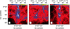 |
Fig. 1 Column density of the selected cloud region viewed from three orthogonal directions. Frame a corresponds to the direction that is selected for the analysis of synthetic observations. The actual 3D spatial separation between the northern and southern density peaks is shown best in frame b (structures in the upper right and lower left part of the plot). |
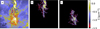 |
Fig. 2 Surface mass density of the whole model cloud (frame a) and separately for the northern and southern clumps (frames b and c). The clumps are defined using a density isosurface at 2 × 105 cm−3, and their outlines are also overplotted in frame a. |
2.3 CASA Simulations
The spectral cubes produced by the radiative transfer calculations were converted to synthetic ngVLA observations with the help of the CASA simulator8. Because our emphasis is on extended rather than sub-core-scale structure, we concentrate on observations made with the Core Subarray, which consists of 94 antennas with maximum baselines of 1.3 km.
The ngVLA observation were simulated with the CASA simobserve script, adding noise according to the published ngVLA characteristics9. The simulated raw observations were also processed with the CASA program, where maps were made with the tclean algorithm, with robust weighting (robust = 0.5) and automatic multi-threshold masking.
The target field was set at zero declination, which results in small ellipticity in the synthesised beam. For the Core antenna configuration, after adding a small amount of tapering, the resolution ranges from 2.6″ × 2.2″ for the ammonia lines near 23.7 GHz to about 0.58″ × 0.50″ for the C18O and 13CO lines near 110 GHz. We used two pointings that are separate by 14″ in the latitude. The corresponding map sizes range from nearly circular ammonia maps, with a diameter of 3.6′, to more elliptical coverage of 0.87′ × 0.77′ at the highest frequencies. This is sufficient to cover the cloud filament that has a length of less than ~0.7′ (0.8 pc at the distance of 4kpc). The nominal simulations correspond to an observing time of six hours with the Core antenna configuration. All observations are corrected for the main beam.
3 Results
3.1 Line Maps
Figure 3 shows maps of integrated intensity for the ideal observations (the direct output from the radiative transfer modelling without beam convolution, observational noise, or the effects of interferometric observations). Apart from differences in the signal level, the molecules (C18O, N2H+ HCO+, and NH3) show only small differences that result from different optical depths and critical densities. The N2H+ and NH3 integrated intensities include the emission from all hyperfine components.
Figure 4 is the corresponding plot for the nominal synthetic ngVLA observations (6 h with the Core array). The noise is sufficiently low not to be clearly visible in the integrated intensity. The main differences compared to Fig. 3 are the loss of some extended emission, for example in the south-west part of the C18O map, which is also visible as lower integrated intensity. There are some regions of negative signal around of the filament. These artefacts might be reduced by more careful manual data reduction and especially by the inclusion of single-dish data. However, at small scales, the correspondence to the ideal maps is good and mainly limited by the beam size of the synthetic observations. Figure 5 shows NH3 and N2H+ spectra that are averaged over parts of the northern and southern clumps where the maximum LOS density exceeds 2 × 106 cm−3 (about half of the areas shown in Fig. 2). In spite of the complex 3D structure of the target areas (see Appendix B), the average spectra are not far from Gaussian.
Figure 6 shows the observed integrated line intensities as a function of column density. The x-axis is here a modified value N′(H2), which is the true model column density scaled with the density dependence that was used in setting the molecular abundances. The density dependence was the same for all molecules. Thus, the actual column density of each molecule is equal to N′(H2) multiplied with the peak abundances of the molecule (Sect. 2.2). In an ideal case, the relationship between W and N′(H2) should be linear.
The first frame of Fig. 6 shows the results for ideal observations. There are minor deviations from linear relationships, with only small effects from temperature (and excitation-temperature) variations and some saturation at the highest optical depths. The same factors affect the dispersion, which is of the order of a factor of two in the direction of the W axis. Figure 6b shows the same for the nominal synthetic ngVLA observations (without single-dish data). The observed W is plotted against the same modified column density N′(H2) as above, but convolved to the angular resolution of the observations. The correlation between column density and integrated intensity W remains fair at the highest column densities, but the observed W values are now lower because of interferometric filtering. The ammonia observations benefit from the lower frequency and the correspondingly larger synthesised beam (lower noise) and larger main beam (larger maximum recoverable scale).
If the line area were plotted against the true column density N(H2) rather than against N′(H2), the W values at the low-column-density part of the plot would appear to drop, although the actual change is in the x-axis variable. The values are lower because the average fractional abundances decrease towards lower column densities. In our case, this amounts to more than a factor of three reduction in the W values at N(H2) ~ 5 × 1021 cm−2, compared to the value seen at N′(H2)) ~ 5 × 1021 cm−2. However, this difference is entirely dependent on the ad hoc assumption of the fractional abundances.
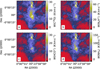 |
Fig. 3 Comparison of integrated intensities W in ideal C18O, N2H+, HCO+, and NH3 observations. |
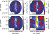 |
Fig. 4 Comparison of integrated intensity W in simulated ngVLA observations (Core antenna configuration with 6 h of observation). As in Fig. 3, the frames show the data for C18O, N2H+, HCO+, and NH3. |
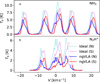 |
Fig. 5 Average ideal and ngVLA-observed NH3 and N2H+ spectra towards the northern (N) and the southern (S) clumps. The dotted lines correspond to ideal observations and the solid lines to the nominal synthetic ngVLA observations. |
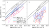 |
Fig. 6 Integrated intensities of selected molecules as a function of N′(H2), which is the true model column density that has been scaled to take into account the density dependence of molecular abundances. Frame a shows the data for ideal observations (full model resolution) and frame b for the simulated ngVLA observations (resolution of ngVLA data). The contours are drawn at 10%, 50%, and 90% of the peak point density (pixels per logarithmic column-density and line-area interval). For HCO+ in frame a, the distribution is plotted also against N(H2), showing the effect of lower average abundances at lower densities. For reference, the dashed black lines show two linear relationships that are separated by a factor of two along the W axis: W = 2 × 10⁻²² × N′(H2) K km s−1 and W = 4× 10⁻²² × N′(H2) K kms−1. |
3.2 Column Densities
Column densities can be estimated with different spectral lines or line combinations (Appendix C). We examine four cases: (1) assuming optically thin C18O lines with Tex = 15 K, (2) using a combination of H13CO+ and HCO+ lines, or using the hyperfine structure of either (3) the N2H+(1−0) or (4) the NH3(1, 1) lines. All estimates are converted to N(H2) by using the maximum fractional abundance in the model cloud. To eliminate the effect of abundance variations, the true model column densities are also re-scaled to take into account the LOS abundance variations, and, once these are convolved to the resolution of the observations, there should ideally be a one-to-one correspondence to the values derived from the synthetic observations.
We fit the spectra with one or more Gaussian components or, in the case of N2H+ and NH3, with the hyperfine structure and one velocity component. Appendix D shows examples of C18O spectra observed towards the northern core that are fitted with different number of Gaussian components. Both the northern and southern cores show a very complex velocity structure, but the relevant line parameters can still be mostly approximated using the single Gaussian. Towards the centre of the field, the emission from the two LOS regions overlaps, and the spectra show two equally strong velocity components that are separated by some 2 km s−1 in velocity.
In Fig. 7, the first column shows the true column density that is modified according to the common density dependence of the abundances. The second column shows the corresponding estimates derived from ideal observations, and the third column the estimates based on the synthetic ngVLA observations. The analysis is based on Gaussian fits or, in the case of N2H+ and NH3 lines, hyperfine fits, all with a single fitted velocity component. There are already significant differences between the first two columns that are caused by the assumptions of the columndensity estimation: LOS homogeneity, the fixed Tex value in the case of C18O, and the inaccuracy of representing the spectra with single Gaussian velocity components.
Figure 8 plots the column-density estimates from C18O, N2H+, and NH3 against the true column density. The plots include estimates from both the ideal observations and the synthetic ngVLA observations. The ideal C18O observations provide accurate values, the adopted Tkin = 15 K not resulting in a significant offset. Bias appears only at high column densities, N(C18O) > 1016 cm−2, where the lines are no longer optically thin or possibly because the Tkin values of the model cloud are systematically lower in regions of high density. In contrast, the ngVLA estimates are clearly lower, mirroring the trends in Fig. 6. Gaussian fits with two velocity components usually result in only small changes, except for some low-column-density regions.
For N2H+, synthetic ngVLA observations reach high S/N only in the high-density part of the filament (Fig. 7i) and the estimates are below the true values. For NH3, the beam size is larger (2.4″ compared to 0.64″ for N2H+), the S/N (and the main-beam size) is similarly larger, and the ngVLA observations provide more accurate estimates up to the highest column densities. At ammonia column densities ~1015 cm−2 and below, the estimates fall below the true values. This is probably due to the filtering of large-scale emission, although the assumption of a single velocity component may also bias the results in some regions.
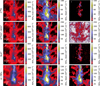 |
Fig. 7 Comparison of true and estimated column densities. The three columns correspond to the true column density, the column density estimated from ideal observations, and the column density derived from the nominal synthetic ngVLA observations. Results are shown for C18O (first row; optically thin approximation), combination of H13CO+ and HCO+ lines (second row), N2H+ (third row; fit of hyperfine structure), and NH3 (bottom row; fit of hyperfine structure). Observational estimates have been scaled to N(H2) using the maximum fractional-abundance value in the modelling. In the first column, the true column densities are also correspondingly scaled down according to the spatial variation of the relative abundances. |
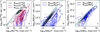 |
Fig. 8 Correlations between column density estimates and the true column density. The y-axis shows the ideal and simulated ngVLA estimates, and the x-axis the true model column density of the molecule in question. Results are shown for C18O, N2H+, and NH3. These correspond to the maps in Fig. 1, with the addition of C18O estimates based on the fitting of two Gaussian velocity components (NCASA2 in frame a). There are nine linearly spaced contour levels, up to the maximum point density (pixels per logarithmic intervals of true and observed column density). |
3.3 Kinetic Temperature
We estimated the gas kinetic temperature with the combination of NH3(1,1) and NH3 (2,2) lines (Appendix C). The analysis assumes a homogeneous and isothermal medium, but the observations should give a good approximation for the mass-weighted temperature, as long as the LOS variations and the optical depths are not extreme (Juvela et al. 2012a).
We used hyperfine fits of the NH3(1, 1) line and Gaussian fits of the NH3(2, 2) line, assuming a single velocity component. Figure 9 compares the true density-weighted kinetic temperature  of the model cloud with the values derived from ideal and from synthetic ngVLA ammonia observations. All data are convolved to 3″ resolution.
The ideal NH3 observations result in correct values to within a couple of degrees, with a small positive bias across all temperatures. In the centre of the map, the presence of multiple velocity components can also contribute to the differences. For synthetic ngVLA observations, the locus coincides with that of ideal observations. However, there is some positive bias at higher temperatures (mostly lower column densities). The maps suggest that these deviations are associated with the border regions with lower S/N, especially for NH3 (2,2), and large-scale effects from the filtering of extended emission.
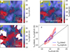 |
Fig. 9 Comparison of kinetic-temperature estimates. The frames show (a) true density-weighted and LOS-averaged kinetic temperature |


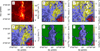 |
Fig. 10 Comparison of mass-weighted average LOS velocity 〈υLOS〉 of the model cloud and the mean radial velocity 〈υ〉 from ideal observations or from synthetic ngVLA observations. Frames show (a) true column density, (b) 〈υ〉 in ideal C18O observations, (c) 〈υ〉 in ideal N2H+ observations, (d) 〈υLOS〉 convolved to 0.55″ resolution, (e) 〈υ〉 in synthetic ngVLA C18O observations, and (f) 〈υ〉 in synthetic ngVLA N2H+ observations. The contour is drawn at column density N(H2) = 5 × 1022 cm−2, and regions of lower column density are masked in frames e and f. |
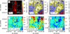 |
Fig. 11 Comparison of radial-velocity estimates from ideal C18O line observations. The frames show: (a) true column density of the model, (b) true mass-weighted average LOS velocity 〈υLOS〉 of the model, (c) mean radial velocity in non-LTE spectra, (d) difference between the radial velocity of the non-LTE spectra and 〈υLOS〉, (e) velocity difference between non-LTE and LTE spectra (including Tkin variations), and (f) velocity difference between non-LTE and LTE spectra, the latter assuming a constant kinetic temperature of Tkin = 15 K. All data are used at full resolution, without beam convolution. |
3.4 Cloud Kinematics
Regarding the cloud kinematics, we look first at the differences between the true mass-weighted average LOS velocity in the model cloud and the mean velocities estimated from line observations. Second, we look at infall indicators and how they are related to the actual infall motions in the model cloud.
3.4.1 Small-scale Velocity Field
We compare the observed mean line velocities 〈υ〉 to the massand abundance-weighted LOS velocity 〈υLOS〉. The observed 〈υ〉 are calculated as the intensity-weighted average radial velocity over the line profiles, both for the ideal spectra and the synthetic ngVLA spectra. The parameter 〈υLOS〉 is read directly from the 3D model cloud. We include in its definition also the abundance variations, so that ideally 〈υLOS〉 ≈ 〈υ〉 for optically thin emission.
Figure 10 compares the observed 〈υ〉 of the C18O and N2H+ spectra to the actual 〈υLOS〉 values in the model. The observed 〈υ〉 values differ from 〈υLOS〉 by up to ~1 km s−1. These can be caused by temperature variations that affect the observed spectra but not the 〈υLOS〉 values. A second explanation are radiative transfer effects, because both C18O and N2H+ reach optical depths slightly above one. The radial velocities derived from the two species are clearly correlated, but also show differences below 1 km s−1. Although synthetic ngVLA observations may be affected by the interferometric filtering, their 〈υ〉 values are still clearly closer to the velocities of the ideal spectra than to the mass-weighted average velocities 〈υLOS〉 of the model cloud.
Figure 11 compares radial velocities of different types of idealised spectra. It shows that the differences between non-LTE spectra and 〈υLOS〉 are explained more by the variations in kinetic temperature (frame f) than by non-LTE effects (frame e). Together these account for about for half of the differences to 〈υLOS〉, self-absorption and other radiative-transfer effects providing further contributions.
Figure 12 shows the same data in the northern core. There are several interesting kinematic features, such as a linear vertical filament (south of the central core, with a length of ~0.05 pc and a width of 0.001 pc) and spiralling structures close to the core centre, which itself shows velocity differences of more than 4 km s−1 between its northern and southern parts. The area of the vertical filament shows a particularly large difference between 〈υLOS〉 and the 〈υ〉 values derived from the non-LTE spectra. The structure almost completely disappears in the latter, because of its low excitation compared to other material along the LOS.
Figure 13 compares further the ideal and synthetic H13CO+ observations of the northern core. The radial velocities are taken from Gaussian fits with a single velocity component10, and they are traced along four paths starting at the core location. The ngVLA observations follow the results of ideal observations, typically with a precision to a fraction of 1 km s−1. Towards the core, limited by the resolution of the observations, the velocity gradients increase up to ~50 km s−1 pc−1. However, large gradients are seen also further out, as the selected path crosses different LOS emission regions. The complexity of the LOS structure is demonstrated further in Appendix B, where we show plots of the 3D density cube and the position–position–velocity (PPV) cube derived from synthetic ngVLA observations of the13 CO line.
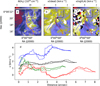 |
Fig. 13 Comparison of radial-velocity estimates from ideal and synthetic ngVLA observations of H13CO+(1−0). Frames a–c show, respectively, the true column density, the radial velocity from ideal observations, and the radial velocity from synthetic ngVLA observations. Frame d shows the radial velocity along the four paths (starting at the core location) indicated in frames a–c. The radial velocity from ideal observations is plotted with solid lines and the velocity from synthetic ngVLA observations with dashed lines. |
3.4.2 Large-scale Velocity Field
Principal component analysis (PCA) uses the eigenvalue decomposition of the spectral observations to examine velocity fluctuations as a function of scale (Heyer & Schloerb 1997) This usually results in a scaling relation δυ ~ Rα, which can be further related to the energy power spectrum (Brunt & Heyer 2002, 2013).
Figure 14 shows the calculated scaling relations for 13CO and C18O, for an area of 27″ × 41″ centred on the filament. In ideal observations, both molecules give the same value of 0.78 for the exponent of the scaling relation, in spite of the optical depths differing by a factor of several (fractional-abundance ratio of 10). The slopes are significantly steeper for the synthetic ngVLA observations, with little difference between the 13CO and C18O lines. The downturn and truncation of the relationships around 0.004 pc is due to the beam size (0.55″ ~ 0.001 pc).
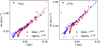 |
Fig. 14 Results of PCA analysis of ideal and synthetic ngVLA observations of the 13CO and C18O lines. The quoted exponents of the scaling relation correspond to least-squares fits to the filled symbols. |
3.4.3 Infall Indicators
The main structure of the model cloud consists of the northern and the southern clumps. These have complex 3D velocity fields, but the net flow of gas is directed towards the clump centres and many individual cores. However, observations provide information only of the LOS velocities. To characterise the corresponding LOS motions in the 3D model, we define an inflow index ξ with the equation
 (1)
(1)
where υ(x) and n(x) are the velocity and the density along the LOS coordinate x. The location of the main LOS density maximum is x0, the radial velocity at that position is υ0, and the sign is selected so that infall towards the maximum corresponds to positive ξ values, the ξ parameter having units of velocity. The averaging can be done over the whole LOS but, to measure gas motions above a given density threshold n0, we use n′ = max(0, n(x) − n0).
Figure 15 shows the ξ values for the whole filament area, for the threshold values of n0 = 104 cm−3 and n0 = 106 cm−3. The high-density gas shows almost exclusively positive ξ values (especially in frame d), indicating the systematic contraction of the structure. When the clumps are examined in more detail, larger ξ values can be resolved towards the central cores at subarcsecond scales (Fig. 16). The mean values of ξ are clearly positive, but there are also small intertwined areas with negative ξ values. When observed at lower resolution, these can be thus expected to dilute the overall infall signature.
In line observations, infall regions might be identified with analysis of the line profiles, with the comparison of optically thin and thick tracers. This presumes that the excitation temperature increases towards the infall centre, which then leads to asymmetric self-absorption and the net emission of optically thick lines moving to lower radial velocities and results in a blueshifted profile. The assumption is likely to be correct for isolated, symmetric, and centrally concentrated structures, rendering it very useful in the study of isolated cores. However, if the line profile contains emission from completely separate LOS structures (with different radial velocities and excitation conditions), the line profile cannot be expected to be closely correlated with the infall motions of individual cores.
We examined this question using a parameter,
 (2)
(2)
that compares the radial velocities of one optically thin and one optically thick line (cf. Mardones et al. 1997), adopting a convention where positive values of δυ indicate infall or collapse. We calculated δV for three pairs of lines: C18O(1−0) and 13CO(1−0), H13CO+(1−0) and HCO+(1−0), N2H+(1−0) and HCO+(1−0). Two alternative sets of input values were used in Eq. (2). In the first case, the velocities and the line width were obtained from Gaussian fits with a single velocity component. In the second case, we examined directly the channels with optically thin emission above a given brightness-temperature threshold and estimated υthin and υthick directly as weighted averaged over these channels.
Figure 17 shows the results for ideal C18O(1−0) and 13CO(1−0) observations. For comparison, we plot in Fig. 17 also the skewness of the 13CO(1−0) profile (for channels around the peak of the C18O(1−0) spectrum).
The values of δυ remain well below δυ ~ 2 that has been considered significant in studies of protostellar cores (Mardones et al. 1997). This is due to the very large total linewidths. The two methods to compute δυ do mostly agree, but there are also areas where the Gaussian fits lead to clearly different or even opposite results. This is not surprising, considering the complexity of some of the spectral profiles. There is very little correlation between the δυ and the ξ values of Fig. 16, and there are marked differences also between the δυ maps derived from ideal observations (Fig. 17) or from the synthetic ngVLA observations (not shown).
The scenario where δυ is able to probe collapse (an isolated core with centrally peaked Tex distribution and a symmetric velocity field) will also result in positive kurtosis in the profiles of optically thick lines. The correlation between kurtosis and δυ is weak for the ideal observations but becomes significant in the synthetic ngVLA observations. This shows that these statistics are not efficient in localising regions of infall motion, not only because of the more complex physical situation but also because they are sensitive to systematic errors that affect the data at larger scales (e.g. self-cancellation due to the extended emission from optically thick species).
We examine the LOS emission further in Appendix B. There the spectra are seen consist of emission from a number of disjoint density peaks, making δv insensitive to actual infall motions in any single LOS density peak. We return to this question also in the following discussion (Sect. 4.5).
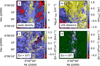 |
Fig. 15 Maps of infall index ξ computed from the 3D model. Upper frames show the peak density along each LOS (frame a) and the distance (relative to the cloud centre) to that location along the LOS (frame b). The lower frames show the ξ maps for density thresholds n0 = 104 cm−3 and n0 = 106 cm−3. The dark green colour corresponds to masked areas where the maximum density along the LOS falls below the density threshold n0. |
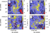 |
Fig. 16 Maps of infall index ξ towards the cores. Upper frames show maps of the peak LOS density towards the northern (frame a) and the southern (frame b) core. The lower frames show the corresponding maps of the infall index ξ, which are computed using a threshold value of n0 = 104 cm−3. |
4 Discussion
We have investigated the use of line observations for studies of star-forming clouds, comparing ideal and synthetic observations to the known properties of the model cloud. In particular, we have simulated observations for the planned ngVLA radio interferometer. We discuss below the main result.
4.1 Cloud Model and Synthetic Observations
The model cloud has a mass of some 3000 M⊙ in a volume of (4 pc)3. It has thus a mean density of nearly n(H2) = 700 cm−3 and is capable of SF up to high-mass stars (Haugbølle et al. 2018). We concentrated on the densest part of the, where the column densities reach up to N(H2) ~ 1024 cm−2. The target is thus similar to a small filamentary infrared IRDC (e.g. Jiménez-Serra et al. 2014; Barnes et al. 2021; Liu et al. 2022). As shown by Fig. 1, the appearance of a single filament can easily result from projection effects in a turbulent cloud (Juvela et al. 2012b). It is noteworthy that in two out of the three orthogonal view direction the same disjoint 3D regions align to form a single filamentary structure. They also have a velocity difference only of a couple of km s−1 and thus cannot be easily separated even in velocity space. The cloud also includes several hundred newly born stars that provide local heating and increase the LOS temperature variations. The average temperatures are low (with a mode of 14.3 K) but exceed 100 K in small regions. Therefore, the model provides a good analogue for a high-mass star forming region with some of its observational challenges.
Nevertheless, there are limitations to the realism of the cloud model. First, it does not include a detailed description of molecular outflows that could considerably further complicate the kinematics. Second, the chemical abundances were set using an ad hoc density dependence, instead of detailed time-dependent chemical modelling. Third, the computed dust temperatures were used as a proxy for the gas temperatures, instead of direct computation of the gas thermal balance. This is justified at high densities (Sect. 2.2) but is increasingly inaccurate when densities fall below ~105 cm−3.
The gas heating varies depending on the local conditions, also in ways that are not considered in our model. Cosmic-ray fluxes in excess of ξ = 10−14 s−1 have been observed towards some high-mass star-forming regions. These are much higher than the typical values in dense clouds (~10−17 s−1 and above, Caselli et al. 1998; Gerin et al. 2010). However, the high rates are found preferentially in regions of low density and low molecular abundances (Bayet et al. 2011). Cosmic rays are attenuated only by thick columns of gas (N(H2) ~ 1023 cm−2) but are also affected by the magnetic fields. Owen et al. (2021) investigated cosmic-ray propagation in filamentary clouds and the resulting effects on gas temperatures. The effect reaches almost 20 K, when the cosmic-ray energy density is increased a factor of ten above its normal Milky-Way value. However, those calculations correspond to lower densities and therefore do not include the gas–dust coupling. In models, where the gas would be heated to similarly high temperatures via photoelectric effect, the collisions are able to bring the gas temperature down to within some degrees of the dust temperature (Goldsmith 2001; Juvela & Ysard 2011). Therefore, although the gas temperatures in our model are not calculated precisely, they are still representative of the temperature fields in real clouds.
More locally, the formed high-mass stars create photon dominated regions (PDRs) and the young stars can produce X-rays with distinct effects on the chemistry (Hollenbach & Tielens 1997; Spaans & Meijerink 2005; Meijerink et al. 2006). The modelling of the detailed temperature structure and chemistry of PDRs is clearly beyond the scope of this paper. The MHD simulation contains a few bona fide massive stars, but, in their surroundings, the predicted line emission will be more reminiscent of earlier evolutionary stages. The selected angular resolution (1″ corresponding to 4000 au) means that the synthetic observations are not sensitive to structures at the scale of protostellar disks.
The above factors do not directly affect our main goal, the comparison of a 3D model and synthetic observations made of that model. Both the column-density and temperature distributions are similar to those found in real IRDCs. Furthermore, the synthetic line observations were calculated with full radiative transfer calculations, which take into not only the varying densities and kinetic temperatures but also deviations from LTE conditions.
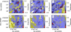 |
Fig. 17 Collapse indicators δV based on ideal C18O and 13CO observations. The upper and lower frames show, respectively, the northern and the southern clumps, for the same area as in Fig. 16. Frames a and d show δυ(proflle) that is computed from channels around the peak of the C18O spectrum. Frames b and e show the corresponding δυ (Gaussian) that is based on line parameters from Gaussian fits. For comparison, frames c and f show the skewness of the 13CO line profiles. |
4.2 Column Densities
As long as the observed lines are not completely optically thick, column densities can be estimated using a single line with an assumed excitation temperature or with two or more lines with an assumed or measured opacity ratio. The cases of the N2H+ and NH3 column densities fall into the second category, making use of the known the optical-depth ratios of the hyperfine components. All our column-density estimates include the assumption of a homogeneous medium, and the resulting errors can be expected to increase as the optical depths and the density and kinetic-temperature variations increase.
Because of the low average kinetic temperatures, the brightness temperatures are in our simulations typically only of the order of 10 K. High sensitivity is therefore required to reliably measure the line intensities outside the densest cores, especially in the case of the N2H+ and NH3 satellite lines. Of these two species, the NH3 integrated intensities are 2-3 times larger (Fig. 3). The largest differences between N2H+ and NH3 are caused, however, by the almost factor of four difference in frequencies. As a result, S/N of NH3 is much higher but the angular resolution is correspondingly lower (2.43″ vs. 0.64″; Fig. 7). Both species provide accurate column density estimates in ideal observation. In the synthetic ngVLA observations, N2H+ shows a larger dispersion (for a significantly higher angular resolution) and systematically lower values (Fig. 8). The low values are naturally explained by the filtering of extended emission, which is evident for example in Fig. 3. Similar to N2H+, reliable observations of C18O and H13CO+ are limited to regions of highest column density (N(H2) ≳ 5 × 1022 cm−2). Previous observations of IRDCs have shown that H13CO+(1−0) emission matches continuum emission quite well in dense regions (Liu et al. 2022).
For the ngVLA Core antenna configuration, the maximum recoverable scales are almost 80″ at the frequency of the NH3(1, 1) line and slightly less than 20″ at the frequency of the N2H+(1−0) line. Our cloud falls between these scales, the filament (N(H2) > 5 × 1022 cm−2) extending over an area of some 40 × 10 arcsec. As pointed out in ngVLA memos11, at scales above 5″ it becomes important for image fidelity and sensitivity to combine interferometric observations with data from a large single-dish telescope. We return to the importance of single-dish data in Sect. 4.6.
We estimated column densities also with C18O(1−0) spectra and the assumption of a constant excitation temperature. For ideal observations, this resulted in fairly accurate estimates, the break-up of the assumption of optically thin lines causing significant underestimation only at the highest column densities (Fig. 8a). However, in our cloud model also the kinetic temperature tends to decrease with increasing density, which could explain part of the bias. In the case of synthetic ngVLA observations, the column densities are underestimated, similar to the N2H+ results, confirming that the bias is common for observations towards the upper end of the ngVLA frequency range and related to the lack of information of the lowest spatial frequencies.
Column densities were calculated using Gaussian fits or, in the case of hyperfine structure, a set of Gaussians for the hyperfine components but only a single velocity component. It is difficult to predict, how much error the Gaussian approximation produces, because this can depend even on the initial values used in the fits. The fitted component might cover multiple velocity components or could converge to just one of those. The effect on C18O column-density estimates is easy to understand, because these are directly proportional to the integrated line intensity. Even in the case of multi-modal spectra (examples shown in Fig. D.1), the differences between the one-component and two-component fits were small at high column densities (Fig. 8). At lower column densities, the two-component fits resulted in larger column densities, by up to a factor of two. Such differences could be expected in the centre of the field, where the spectra show two equally strong velocity components.
The hyperfine structure of the N2H+ and NH3 lines was fitted using only a single velocity component. Unlike in the simple Gaussian fits, these fits provide directly estimates for the excitation temperature and optical depth. In this case, multi-component fits could easily lead to unphysical solutions. For example, one components could have Tex < Tbg, providing an ‘absorption’ feature to help the fitting of some non-Gaussian line profiles, or one could even have Tex ≈ Tbg combined with an arbitrary column density. Some unphysical solutions could be automatically rejected or avoided by using suitable regularisation. However, fitting of multi-component models to hyperfine spectra remains susceptible to degeneracies, and the automatic selection of the physically most likely solution remains a challenge. In the purely technical sense, the fits are still easy. For example, the maps of ideal observations in Fig. 7 contained some 5 million individual spectra but could fitted in just a few minutes.
4.3 Estimates of Kinetic Temperature
Figure 9 showed kinetic-temperature estimates derived from the NH3(1, 1) and NH3(2, 2) spectra. The accuracy of the estimates obtained with synthetic ngVLA observations is mostly comparable to that of ideal observations, with statistical noise of the order of 1 K. However, there is an increasing positive bias towards higher temperatures, which mirrors the behaviour in Fig. 8c for N(H2) at low column densities. This can be attributed partly to imperfections of the fits (with a single velocity component) and the different optical depths of the transitions, when combined with the large LOS temperature and density variations. Shirley (2015) estimated that the effective critical density of the NH3(2, 2) is at 10–20 K temperatures about two times higher than that of NH3(1, 1). In the Tkin analysis, the NH3(2, 2) spectra were fitted using fixed radial velocities obtained from the NH3(1, 1) hyperfine fits. If the radial velocities of the NH3(2, 2) line are kept as free parameters, the appearance of Fig. 9 changes only little, which shows that the two transitions are still essentially probing the same volume of gas. The temperature determination may also be influenced by imperfections in the interferometric observation and the data reduction, larger self-cancellation in NH3(1, 1) observations naturally leading to positive bias in Tkin estimates. The S/N of the synthetic ngVLA observations was clearly sufficient to map kinetic temperature over large cloud areas, beyond the N(H2) = 5 × 1022 cm−2 threshold used in Fig. 9.
4.4 Velocity Fields
Analysis in Sect. 3.4.1 showed that the mean radial velocity of observed spectral lines can significantly differ from the actual mass-weighted mean radial velocity in the model cloud. For ideal observations, which were computed at the full resolution of the model, the differences were up to ±1 km s−1. This corresponds to a large fraction of the total range of velocities. The total velocity dispersion of our model cloud is ~4 km s−1, which is also consistent with observations of many IRDCs (Li et al. 2022; Liu et al. 2022). The large differences between the observed and true (mass-weighted) velocities are limited to small regions, typically with large volume densities and large optical depths. The synthetic ngVLA observations and ideal line observations show differences at two distinct scales. At the smallest scales, close to the resolution of the observations, these result from observational noise. In the area with N(H2) > 5 × 1022 cm−2, the rms differences are quite small, ~0.1 km s−1 and ~0.15 km s−1 for C18O and N2H+, respectively. These values were measured at scales below 4″, by filtering out the larger-scale signal in the velocity maps. The absolute differences could be several times higher, but these are limited to larger spatial scales (> 4″) and are observed to be similar for both molecules. Therefore, based on the similar frequencies of the lines, these are most likely related to the filtering of large-scale emission and other imperfections in the imaging procedures.
Further investigations showed that the differences between the radial velocity of spectra and the true gas velocities are caused by temperature variations and optical-depth effects, which change the relative contribution of different LOS regions. The non-LTE effects (i.e. Tex variations in addition to Tkin variations) had a smaller impact (Figs. 11–12). The synthetic ngVLA observations traced well the large-scale velocity structures, from the beam size up to at least ~4″. Thanks to the hyperfine structure, the velocity determination is particularly accurate with N2H+ observations (Fig. 10).
Zooming into the cores, one interesting detail in Fig. 12 is the presence of a filament that is feeding the central core. Although this was clearly identifiable in the 3D model due to its different LOS velocity, it almost completely disappeared in synthetic observations, in the line-velocity maps. This could be attributed to its much lower kinetic (and excitation) temperature. The filament was detected in channel maps (for example in HCO+), but only marginally. This is because the width of the structure is below the beam size and the structure is weak compared to other emission along the LOS. The detectability of such kinematic features should be studied further, especially with models that more accurately describe the temperature and chemical composition of such structures.
The fact that radial velocities measured from synthetic ngVLA observations are close to those in ideal observations will be important for studies of the accretion associated with cores and especially in the context of high-mass SF and hub-filament systems. Figure 13 shows that H13CO+ (1−0) provides accurate measurements of the radial velocity and velocity gradients, as judged by the comparison with ideal observations. This will be important, when gradients are used to detect infall and to estimate infall rates. For example, Zhou et al. (2022) presented ALMA observations of hub-filament systems in a number of proto-clusters. The systematic velocity gradients scales of a few 0.1 pc were up to tens of km s−1, suggesting almost free-fall motions towards the massive hubs. In Fig. 13, 0.1 pc would correspond to ~5″, but the most systematic velocity gradients are seen only close to the resolution limit, in agreement with the lower mass of this system. However, in such complex regions, the estimation of velocity gradients and the corresponding gas-inflow rates is complicated not only by the random inclinations of the structures but also by the presence of many LOS structures that can lead to high apparent and partly artificial gradients. For example, in Fig. 13, the blue path crosses from the diffuse background to a filament, leading to an apparent gradient of close to ~50 km s−1 pc−1 (around the offset of 3″). Gradients should clearly be measured only along well-defined and continuous structures. The risk for artificial gradients, caused by change alignment of LOS structures, may also increase towards the central regions of hub-filament systems.
In Sect. 3.4.2, we looked briefly at the global velocity statistics with the help of the PCA method. The PCA estimates of the δυ ~ Rα scaling relation were well defined and the slopes were almost identical for the 13CO and C18O data, with α = 0.78. The synthetic observations resulted, however, in clearly steeper relationships (α = 1.00 and α = 1.05 for 13CO and C18O, respectively), again suggesting some effect from the interferometric filtering. Of course, for such analysis of large-scale density or velocity fields, the coverage of low spatial frequencies with additional single-dish data becomes crucial (Sect. 4.6). In spite of the S/N differences and the high S/N C18O observations being limited just to the central filament, the 13CO and C18O values were quite consistent with each other.
4.5 Failure of Infall Indicators
We compared the collapse indicator δv of Eq. (2) to the actual LOS flows in the model. The latter were quantified with the parameter ξ, the density-weighted net mass flow towards the highest LOS density peak (Eq. (1)). The comparison of ξ and δυ showed little correlation (Figs. 16 and 17, respectively). This was true even in the case of ideal line observations.
The parameter δυ is based on the picture of a single core, where the excitation temperature increases towards the centre. This leads to an asymmetry, where the optically thick species suffer more self-absorption on its redshifted side, leading to positive values of δυ (with the signs used in Eq. (2)). This is clearly not an appropriate description for more complex regions, where the LOS crosses several density peaks. In this case, δυ depends more on the random superposition of emission from structures with different excitation temperatures and radial velocities. Already in the case of two LOS clumps, the sign of δυ is likely to depend more on their relative velocities than the infall within individual clumps. The same complexity also affects the parameter ξ, but that at least is based on the true velocity field and concentrating on the main LOS density peak.
Appendix B illustrates the complexity of the density and velocity fields for selected sightlines, where large ξ values indicate a particularly strong inflow motion. We examine here the LOS for the fourth core (counted from north) that is indicated in Fig. B.2. Figure 18 shows, how an observed HCO+(1−0) spectrum is composed of the emission and absorption at different locations along the full LOS through the model cloud. In the case of the optically thinner H13CO+, up to 30% of the local emission is absorbed by foreground layers, but the shape of the total spectrum is only little affected by these optical-depth effects. In contrast, HCO+ emission can be completely absorbed by foreground structures, and most of the observed emission originates on the front side of cloud. For individual cores, one can often observe the change from redshifted emission on the near side to more blueshifted emission on the far side. However, several LOS structures contribute to the emission and absorption at any given radial velocity, and the spatial separation of the structures is >0.1 pc, much larger than the size of individual cores. Because of the random radial-velocity offsets between the structures, the observed spectrum does not show clear blue asymmetry.
Figures in Appendix B show further plots on how different LOS structures contribute to different spectral lines. In particular, Fig. B.4 splits a spectrum to its blueshifted and redshifted components in the case of another LOS. Also in that case, the dominant core is consistent with the basic assumptions of the δv diagnostic (redshifted emission on the front side and blueshifted emission on the far side of the core), but this signature is masked by other LOS structures. One similar concrete example was provided by Zhou et al. (2021), who carried out ALMA observations of the high-mass star-forming clump G286.21+0.17. The clump contains a filament that, based on the blue asymmetry of the single-dish HCO+ spectra, had been interpreted to be in global collapse. Interferometric observations revealed two separate clumps, and the asymmetry could be seen to be caused by the relative velocity of the clumps rather than by any systematic infall.
If all LOS structures were at clearly different radial velocities, the δυ statistics might be applied to individual velocity components. However, it is difficult ascertain from observations that one has correctly isolated a single core in velocity space, especially if the object is not fully spatially resolved. Therefore, the δυ-diagnostic will remain more applicable to nearby regions of low-mass SF, where the LOS confusion is lower and the spatial resolution typically higher.
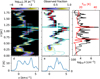 |
Fig. 18 Contributions of different LOS regions to a selected HCO+(1−0) spectrum. In frames a and b, the y-axis corresponds to the distance from the observer’s side of the model cloud, and the x-axis shows the radial velocity. Frame a shows the intensity of the local emission that reaches the observer and thus contributes to the observed spectrum in frame d. Frame b shows the same as the fraction of the local emission that is not absorbed by the foregrounds. The cyan contours are drawn around significant emission, to help the comparison between the frames a and b. In frame b, the observed fraction of emission is plotted only inside the contour. Frame e shows the corresponding fictitious optically thin spectrum, where all foreground absorption is ignored. The LOS variations in density (black curve) and kinetic temperature (red curve) as shown in frame c. |
4.6 Combination of Interferometer and Single-dish Data
Interferometric measurements are usually combined with single-dish data to recover information of large spatial scales (Cornwell et al. 1993). We simulated single-dish N2H+ (1−0) observations for a 8.1″ beam, which corresponds to a 100-m dish such as the Green Bank Telescope (GBT)12. The observational noise was set to 0.1 K, which is realistic for GBT data (Pingel et al. 2021). The single-dish observations were used as a model in the CASA tclean13 procedure, resulting in a spectral cube with information also of the largest scales. As an alternative, we reduced the ngVLA data separately and joined them with the single-dish data with the feathering procedure. These two alternatives should produce comparable results, although in practice differences up to tens of per cent might be observed in individual spectra (Barnes et al. 2021). We used the uvcombine14 tool for the feathering of the ngVLA and single-dish images.
Figure 19 shows the results in terms of column densities and sample spectra at the 0.55″ resolution. The results are very similar, whether the ngVLA and single-dish data are reduced together or joined by feathering. The spectral profiles are identical to within ~10%, and the column densities along the selected stripe are also well correlated. Some larger differences are observed close to the position C, where the wide lines and the presence of multiple velocity components causes problems for our analysis that is based on hyperfine fits with a single velocity component. With the exception of the position C, all observations tend to underestimate the true column density. This in spite of the fact that the latter values are here again corrected for the spatial abundance variations. Excluding the peak N(N2H+) > 2 × 1014 cm−2 around the position C, the differences between the two alternative combinations of ngVLA and single-dish data were ~14%, the feathering resulting in only 5% lower average value. Figure 19 also shows that the difference between the synthetic and the ideal N2H+ observations is smaller than the difference between the ideal observations and the true column densities. This applies both to the mean value and the variations along the selected stripe.
In Sect. 3.2, column densities were calculated using single lines, because the interferometric filtering appeared to have different effect on, for example, the optically thin C18O and the much more extended 13CO emission. After combining ngVLA and single-dish data, Fig. 20 shows correlations between the true column density (obtained directly from the model) and estimates calculated using the C18O versus 13CO and the H13CO+ versus HCO+ line ratios. The situation is much improved over the ngVLA-only results in Fig. 8, but the use of the 13CO versus C18O line ratios results in only marginal improvement over the simpler assumption of optically thin C18O emission. There is also some bias that is still larger in the synthetic observations than in the ideal observations. Rather than having real physical causes, this might thus result from some imperfections in the data reduction or in the inclusion of the single-dish data. Apart from systematic errors, the dispersion is small and mostly below 25%. The plot is limited to within 10″ of the two pointing centres, where the hydrogen column densities are N(H2) ~ 1023 cm−2 or even higher. The estimates calculated from the H13CO+ versus HCO+ line ratio do not show bias, but the increase in dispersion towards lower column densities is more noticeable.
In Fig. 20a, the assumed Tex = 15 K resulted in quite accurate estimates. With Tex = 25 K, the column densities would be overestimated by more than 50%, the effect being almost the same for the whole map. Thus, a single optically thin line can already provide much information on relative structures, and, depending on the science case, the addition of good-quality single-dish data can be more important than the more precise excitation-temperature information obtained from line ratios.
The emission at the brightest parts of the filament was captured quite well already in the ngVLA-only observations. Section 4.4 showed that the same conclusion applies to the velocity fields observed towards the densest sub-structures. Therefore, ngVLA data without any additional single-dish data could be sufficient for studies of the individual densest regions. On the other hand, single-dish data remain essential for extended sources – such as the examined IRDC model – and any studies into the large-scale velocity or density statistics (Sect. 3.2).
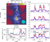 |
Fig. 19 Comparison of N2H+ observations with and without single-dish data. The top left frame shows the N(N2H+) column-density map that is derived from the combined ngVLA and single-dish data. The circle in the lower left corner corresponds to the 0.55″ resolution of the final map, and the circle in the lower right corner shows the 8.1″ beam of the single-dish data. The bottom left frame shows a comparison of the column-density estimates along the path that is plotted in the first frame. Results are shown for ideal observations and for ngVLA and single-dish observations when both are included in the cleaning process (“combined”) or when they are joined afterwards through feathering (“feathered”). We plot also the true column density that is obtained directly from the model cube. The right-hαnd frames show sample spectra towards the four positions marked in the first frame. The spectra from interferometric observations without combined single-dish data (“ngVLA”) are also shown. |
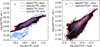 |
Fig. 20 Column-density estimated from C18O versus 13CO (frame a) and H13CO+ versus HCO+ (frame b) line ratios, plotted against the true column density N′(H2) (accounting for the effect of density-dependent fractional abundances). Results are shown for both ideal observations and the combined ngVLA and single-dish data. The diagonal dashed line corresponds to the expected one-to-one relation. For each dataset (listed in the legends) there are four contour levels that are equidistant from close to zero up to 80% of the maximum point density. The background greyscale images correspond to the estimates calculated from ngVLA line ratios. In frame a, the estimates for optically thin C18O emission at Tex = 15 K are shown for comparison. Plots use data within 10″ of the pointing centres and a resolution of 0.7″. |
5 Conclusions
We have simulated observations of a high-column-density molecular cloud to study the foreseen performance of the ngVLA interferometer for studies of the ISM and the early phases of the star-formation process. As the baseline case, we examined observations with the ngVLA Core antenna configuration and a total observing time of 6 h. The comparison of the ngVLA synthetic observations, the corresponding ideal line observations, and the actual 3D cloud model resulted in the following conclusions.
The ngVLA observations described the general structure of the filamentary cloud accurately. In the measurements of the integrated line intensity (e.g. HCO+, N2H+, and NH3), the noise does not become significant even close to the maximum angular resolution (down to ~0.5″).
At high frequencies, observations of our model cloud suffer from some loss of extended emission. For NH3 the effect remains small at the scale of the examined cloud (~15″ × 40″), and the column-density estimates remained accurate to about 30%, even without the use of single-dish data.
The kinetic temperatures derived from NH3 observations were mostly accurate to within ~1 K. However, at lower column densities some positive bias was observed, which could be attributed to some loss of extended signal even at the NH3(1,1) frequency.
The synthetic ngVLA observations provided an accurate image of the kinematics at intermediate scales. For example, velocity gradients associated with the main cores could be traced mostly with a precision better than ~0.3 km s−1. At higher frequencies (e.g. C18O and N2H+ lines), the radial-velocity data show low-spatial-frequency deviations, because the target cloud is larger than the maximum recoverable scale. The loss of low-spatial-scale information is reflected in global statistics, but the effects remained moderate, for example, in the PCA analysis of 13CO (in spite of the very extended emission) and C18O (in spite of the much lower signal-to-noise ratio) lines.
The ngVLA observations traced the kinematics within the cores down to the resolution limit. However, at the smallest scales some important features remain undetectable either because of beam dilution or because their spectral signatures (even in ideal observations) are weak. The emission from some dense regions was masked by the emission and absorption of other LOS regions, either because of temperature differences or radiative transfer effects.
We compared standard collapse indicators to the actual infall motions in the 3D model cloud. The blue asymmetry of optically thick lines was not significantly correlated with actual LOS motions in the cloud. The spectra were complex, containing contributions from many LOS density peaks. This makes it difficult to unambiguously interpret any observed spectral asymmetries in terms of a local collapse.
The addition of single-dish data recovers the lost large-scale emission, and, for example, the synthetic N2H+ spectra were found to be very similar to the ideal observations. However, there can still be significant differences between the true column densities and the estimates, even if these were derived from ideal observations. The complex velocity structure can lead to large errors or even complete failure in the column-density estimation.
The ngVLA will provide precise measurements of the small-scale structure and the physical and chemical state of star-forming clouds, even for high-mass star-forming regions at kiloparsec distances. However, complementary single-dish data remain essential for accurate estimates of the total column density and the large-scale kinematics.
Acknowledgements
E.M. is funded by the University of Helsinki doctoral school in particle physics and astrophysics (PAPU). Tie Liu acknowledges the supports by National Natural Science Foundation of China (NSFC) through grants No. 12073061 and No. 12122307, the international partnership program of Chinese Academy of Sciences through grant No. 114231KYSB20200009, Shanghai Pujiang Program 20PJ1415500 and the science research grants from the China Manned Space Project with no. CMS-CSST-2021-B06. We thank Troels Haugbølle for providing the data for the MHD simulations, and we acknowledge PRACE for awarding access to Curie at GENCI@CEA, France to carry out those simulations.
Appendix A Maps of Dust Emission and Temperature
The line simulations assumed that the kinetic temperature is equal to the dust temperature (Sect. 2). Figure A.1 shows for reference maps of the 250 µm surface brightness and dust colour temperature. The temperatures are estimated with modified blackbody fits to the synthetic 160, 250, 350, and 500 µm surface brightness maps, giving equal weight to data in all four bands. The dust opacity spectral index was assumed to be a constant β=1.8, which is close to the value in the used dust model.
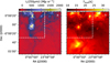 |
Fig. A.1 Maps of dust emission at 250 µm (left frame) and dust colour temperature (right frame). The dashed line shows the area discussed in the main part of the paper. The data correspond to the full resolution of the cloud model (using 0.05″ pixel size for the plot). |
Appendix B Origin of Observed Emission
Figure B.1 shows the main structures of the 3D density field and the kinematic structures seen in the PPV cube of the synthetic 13CO data. The density values were thresholded at n = 5 × 105 cm−3 and the detected regions, each with an individual label, were further extended to the region with n > 3 × 105 cm−3. Regions with fewer than 100 cells were removed, where the cell size corresponded to 0.25″. The 13CO data were analysed using the results from Gaussian fits with up to three velocity components, only using the components with brightness temperatures exceeding 3.5 K. These provide discrete points in the PPV space, where neighbouring points were further connected, if their distance was below
 (B.1)
(B.1)
Here ∆υ and ∆x are the distances along the velocity and spatial coordinates. The scales were set to δυ = 0.2 km s−1 and to δx equal to half of the beam FWHM. Each connected PPV region (velocity-coherent region) was given a unique label. Figure B.1 shows the extracted PPP and PPV regions as stereographic images.
Because the usual collapse indicator δυ showed little correlation with the actual infall motions in the model cloud, we examined further the contribution of different LOS regions to the observed spectra. Figure B.2 shows spectra towards five positions with large ξ values. These all contain several velocity components.
We examine further the northernmost LOS marked with a cross in Fig. B.2. Figure B.3 plots the density, kinetic temperature, and relative abundance along the full LOS. The LOS consist of a number of smaller density peaks, some of which are close in density to the strongest one. The lower frames of Fig. B.2 show the contributions of different LOS regions to the intensity in the observed spectrum. One takes here into account not only the local emission but also how the intensity is attenuated by foreground absorption. There are several density peaks with almost equal contributions to the observed spectra.
In Fig.-B.4, we examine further two pairs of spectra, C18O and 13CO and, on the other hand, H13CO+ and HCO+. We separate the lines to their redshifted and blueshifted parts using the mean velocity of the optically thinner line. The main density peaks (indicated with arrows) are associated with redshifted emission at the front side and blueshifted emission at the back side, which is consistent with collapse motions and agrees with assumptions of the δv diagnostic. However, in the final spectra such local effects are masked by the superposition of emission from many density peaks. This supports a scenario where, even if there were systematic inflow at all scales, the values of δυ will depend more on the relative density, excitation, and radial velocity of individual density structures, rather than the emission asymmetry in individual cores.
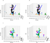 |
Fig. B.1 Stereographic images of the high-density structures (frames a and b) and the PPV structures extracted from synthetic 13CO ngVLA observations (frames c and d). The density structures correspond to regions above n = 3 × 105cm−3 and the PPV structures to individual Gaussian components brighter than 3.5 Κ in brightness temperature. |
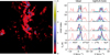 |
Fig. B.2 Spectra for selected LOS with strong inflow motions. The first frame shows the inflow index ξ convolved to 1″ resolution. Crosses mark five locations with large ξ values, and the plots on the right show spectra for these positions (rows in decreasing order of latitude). Spectra in the first column correspond to ideal observations and the spectra in the second column to simulated ngVLA observations. Spectra are plotted for C18O (black lines), HCO+ (blue), H13CO+ (cyan), and N2H+ (dashed red lines). |
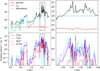 |
Fig. B.3 Parameters along the LOS towards the position indicated by the northernmost cross in Fig. B.2. The first frame shows the density (black line), abundance (arbitrary normalisation and cyan line), and kinetic temperature (red line). Frame b shows same data with a zoom-in to the dashed box in frame a. The bottom frames shows the contributions of different LOS regions to the observed spectra (integrated line intensity). |
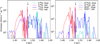 |
Fig. B.4 Same as lower right frame of Fig. B.3 but splitting emission to blueshifted and redshifted parts at the mean velocity of the optically thinner species (C18O in the left and H13CO+ in the right frame). The black arrows indicate the position of the main density peak. |
Appendix C Column Density Estimates
The observed brightness temperatures are
![Mathematical equation: $ {T_{\rm{b}}} = \eta \left[ {{J_v}\left( {{T_{{\rm{ex}}}}} \right) - {J_v}\left( {{T_{{\rm{bg}}}}} \right)} \right]\left( {1 - {e^{ - \tau }}} \right), $](/articles/aa/full_html/2022/10/aa44026-22/aa44026-22-eq11.png) (C.1)
(C.1)
where we assume an efficiency (including beam filling) of η = 1 and a background temperature of Tbg=2.73 K (same as in the radiative transfer simulations), and function J is defined as
 (C.2)
(C.2)
For the NH3(1,1) and N2H+ lines the optical depth τ and the excitation temperature Tex are obtained directly from the fitting of the above equation to the observed spectra, simultaneously including all hyperfine components with their known relative intensities.
Optical depth can also be estimated from the intensity ratio of lines with a known opacity ratio. This is often used with C18O and 13CO lines, and we apply the method to the HCO+ and H13CO+ lines. Assumptions of the same excitation temperature, beam filling, and line width for both lines lead to the expression
 (C.3)
(C.3)
for the ratio of the measured brightness temperatures (Myers et al. 1983). With the assumed ratio r between the optical depths of the two species A and B, the optical depths can be solved.
Once the optical depth τν and excitation temperature Tex are known, the column density of molecules on the upper energy level of the transition can be calculated as
 (C.4)
(C.4)
or, using the peak optical depth τ0 and FWHM line width ∆υ from Gaussian fits,
 (C.5)
(C.5)
The total column density of the molecules is obtained by scaling with the ratio of the sum of populations on all energy levels relative to the population of the level u,
 (C.6)
(C.6)
assuming the same excitation temperature for all transitions. Here gi are the statistical weights and Ei the energies of the energy levels, and Q is the partition function.
If the emission is optically thin, column density estimates can be written in terms of an assumed excitation temperature Tex and the integrated line intensity W,
 (C.7)
(C.7)
(Caselli et al. 2002b). We use this in calculations based on Gaussian fits, where
 (C.8)
(C.8)
In particular, for the J = 1 → 0 transition of C18O, Mangum & Shirley (2015) provide the formula
![Mathematical equation: $ {N_{{\rm{tot}}}}\left( {{{\rm{C}}^{18}}{\rm{O}}} \right) = {{2.48 \cdot {{10}^{14}}\left( {{T_{{\rm{ex}}}} + 0.88} \right){e^{{T_0}/{T_{{\rm{ex}}}}}}\smallint {T_b}dv\left( {{\rm{km/s}}} \right)} \over {\eta \left[ {{e^{{T_0}/{T_{{\rm{ex}}}}}} - 1} \right]\left[ {{J_v}\left( {{T_{{\rm{ex}}}}} \right) - {J_v}\left( {{T_{{\rm{bg}}}}} \right)} \right]}}, $](/articles/aa/full_html/2022/10/aa44026-22/aa44026-22-eq19.png) (C.9)
(C.9)
where  . Similarly, for optically thin N2H+ emission
![Mathematical equation: $ {N_{{\rm{tot}}}}\left( {{{\rm{N}}_2}{{\rm{H}}^ + }} \right) = {{6.25 \cdot {{10}^{15}}{e^{{T_0}/T}}\left( {{T_b}/{R_i}} \right)\Delta v} \over {v\eta \left[ {{e^{{T_0}/T}} - 1} \right]\left[ {{J_v}\left( {{T_{{\rm{ex}}}}} \right) - {J_v}\left( {{T_{{\rm{bg}}}}} \right)} \right]}}\left[ {{\rm{c}}{{\rm{m}}^{ - 2}}} \right]. $](/articles/aa/full_html/2022/10/aa44026-22/aa44026-22-eq21.png) (C.10)
(C.10)
In these formulas, frequency ν is given in gigahertz and the line width ∆υ in kilometres per second, and the result is the column density per square centimetre. In the N2H+ equation, Tb refers to the brightness temperature of one of the hyperfine components, which is then scaled with the relative intensity Ri of that component (ΣiRi ≡ 1). However, if the line is not optically thin, one can estimate Tex and τ by a simultaneous fit to all hyperfine components, as mentioned above.
The hyperfine fit to ammonia NH3(1,1) spectra also provides Tex and τ. Assuming Gaussian line parameters, the integration of optical depth profile gives
 (C.11)
for the column density of the upper level, with T0 = 1.14 K, the line width ∆υ being included in kilometres per second (Harju et al. 1993). As in the case of N2H+, if the emission is too weak for the hyperfine fit, column density can still be estimated from the integrated brightness temperature that is assumed to be optically thin,
![Mathematical equation: $ {N_u} = {1 \over \eta }\xi {1 \over {1 - {{\exp \left( {{T_0}/{T_{{\rm{ex}}}}} \right) - 1} \over {\exp \left( {{T_0}/{T_{{\rm{bg}}}}} \right) - 1}}}}\int {{T_b}dv} \,\,\,\left[ {{\rm{c}}{{\rm{m}}^{ - 2}}} \right]. $](/articles/aa/full_html/2022/10/aa44026-22/aa44026-22-eq23.png) (C.12)
(C.12)
The NH3(2, 2) transition can be handled in the same way, integrating only over the main component. The numerical factor ξ is 1.3 · 1013 for the NH3(1,1) and 6.2 · 1012 for the NH3(2,2) line. The total column density of NH3(1,1) is obtained as the sum of populations on the upper and lower level,
 (C.13)
The rotation temperature T12 is obtained from the column density ratio
 (C.14)
Walmsley & Ungerechts (1983) provide the transformation from T12 to kinetic temperature, based on a three-level model of the (1,1), (2,2), and (2,1) levels of para ammonia. Finally, the total ammonia column density can be estimated as
 (C.15)
assuming that only metastable levels are populated and the ortho/para ratio is thermalised (Ungerechts et al. 1986; Harju et al. 1993).
Appendix D Fits of Spectral Profiles
Most of the analysis was based on Gaussian fits or, in the case of N2H+ and NH3, simultaneous fitting of all hyperfine components and assuming a single velocity component. All Gaussian fits were also repeated with up to three velocity components. The calculations were made by our own GPU-accelerated fltting routine, with approximately 1 ms run time per spectrum (less for single-component Gaussians, slightly more in case of multiple velocity components or hyperfine spectra). In Sect. 4.6, the pyspeckit program (Ginsburg & Mirocha 2011) was used for comparison and to confirm the correct performance of our own routine.
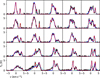 |
Fig. D.1 Examples of Gaussian fits towards the northern core, for simulated C18O observations (black lines) with the ngVLA Core configuration. The fits with one, two, and three Gaussian components are plotted with cyan, blue, and red lines, respectively. The spectra are taken at steps of FWHM, equal to 0.54″. |
When the spectra contain multiple velocity components, a fit may converge to a wrong solution, failing to fit the main velocity feature or, in fits with NC velocity components, failing to fit the NC most important features. Each fit was therefore repeated four times, using different initial parameter values and keeping the results from the fit with the lowest χ2 value. Figure D.1 shows examples of the fits of C18O spectra towards the northern core, using 1-3 velocity components. Not all fits are perfect (e.g. three-component fits sometimes missing one of the three most important features, like in the second frame of the plot). On the other hand, even the single-component fits usually approximate the total emission well, biasing the column-density estimates by much less than 50%.
The presence of multiple velocity components presents problems especially for hyperfine fits, because, without additional constraints, some components might converge to an unphysical solution (e.g. a combination of a very low Tex and a very large optical depth). This is not possible in the case of a single component that alone must match the observed spectrum. Conversely, if a spectrum that contains multiple velocity components is fitted with a model that contains only a single velocity component, the results are again biased. Figure D.2 shows, how the recovered optical depth and column density depend on the velocity difference between two equally strong velocity components. In this example, the original optical depth (the sum of the hyper-fine components) is ten, and the velocity difference is increased from zero to 4.0 km s−1. The two components both have (before optical-depth effects) a line width of ∆υ =1.0 km s−1. As the velocity components move further apart and the fitted spectrum falls between them, the optical depth is increasingly underestimated. On the other hand, the estimated column density, which also depends on both Tex and ∆υ, remains remarkably accurate.
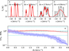 |
Fig. D.2 Test of fitting N2H+ observations containing two velocity components. The upper frames show simulated spectra (black lines) with 0.3 K observational noise and varying velocity difference δυ between the two components. Fits of a single velocity component are plotted in red for a number of noise realisations. The lower frame shows the recovered optical depth (blue line) and column density (red line) as a function of the velocity offset δυ. The shaded regions correspond to the inter-quartile range, which is computed from 128 noise realisations. The y-axis shows the ratio between the estimates and the true values. |
For large velocity differences, δυ ≳ 2 km s−1, we occasionally saw alternative fits that indicated much higher optical depths. These can be understood as an attempt to match the two velocity components with a single wide, flat-topped (i.e. completely saturated) spectral profile. These solutions tended to have higher χ2 values than the low-τ solutions, such as shown in Fig. D.2, suggesting that the alternative solutions might be caused by poor convergence or a local χ2 minimum. The differences in the χ2 values between the good and the alternative worse fit was only at 10% level. Therefore, one might encounter more of such bad fits (although possibly corresponding to a global χ2 minimum) when the signal-to-noise ratio of the observations is lower. They would then result in both the optical depth and the column density to be overestimated, potentially even by a factor of several.
References
- Areal, M. B., Paron, S., Celis Peña, M., & Ortega, M. E. 2018, A&A, 612, A117 [NASA ADS] [CrossRef] [EDP Sciences] [Google Scholar]
- Areal, M. B., Paron, S., Ortega, M. E., & Duvidovich, L. 2019, Publ. Astron. Soc. Austr., 36, e049 [CrossRef] [Google Scholar]
- Barnes, A. T., Henshaw, J. D., Fontani, F., et al. 2021, MNRAS, 503, 4601 [CrossRef] [Google Scholar]
- Bayet, E., Williams, D. A., Hartquist, T. W., & Viti, S. 2011, MNRAS, 414, 1583 [NASA ADS] [CrossRef] [Google Scholar]
- Beuther, H., Gieser, C., Suri, S., et al. 2021, A&A, 649, A113 [NASA ADS] [CrossRef] [EDP Sciences] [Google Scholar]
- Blake, G. A., Sutton, E. C., Masson, C. R., & Phillips, T. G. 1987, ApJ, 315, 621 [Google Scholar]
- Bonnell, I. A., Bate, M. R., Clarke, C. J., & Pringle, J. E. 2001, MNRAS, 323, 785 [Google Scholar]
- Bonnell, I. A., Vine, S. G., & Bate, M. R. 2004, MNRAS, 349, 735 [Google Scholar]
- Brunt, C. M., & Heyer, M. H. 2002, ApJ, 566, 289 [NASA ADS] [CrossRef] [Google Scholar]
- Brunt, C. M., & Heyer, M. H. 2013, MNRAS, 433, 117 [NASA ADS] [CrossRef] [Google Scholar]
- Caselli, P., Walmsley, C. M., Terzieva, R., & Herbst, E. 1998, ApJ, 499, 234 [Google Scholar]
- Caselli, P., Benson, P. J., Myers, P. C., & Tafalla, M. 2002a, ApJ, 572, 238 [Google Scholar]
- Caselli, P., Walmsley, C. M., Zucconi, A., et al. 2002b, ApJ, 565, 344 [Google Scholar]
- Chira, R. A., Beuther, H., Linz, H., et al. 2013, A&A, 552, A40 [NASA ADS] [CrossRef] [EDP Sciences] [Google Scholar]
- Cornwell, T. J., Holdaway, M. A., & Uson, J. M. 1993, A&A, 271, 697 [NASA ADS] [Google Scholar]
- Csengeri, T., Bontemps, S., Schneider, N., Motte, F., & Dib, S. 2011, A&A, 527, A135 [NASA ADS] [CrossRef] [EDP Sciences] [Google Scholar]
- Dickman, R. L. 1978, ApJS, 37, 407 [CrossRef] [Google Scholar]
- Du, F., & Yang, J. 2008, ApJ, 686, 384 [NASA ADS] [CrossRef] [Google Scholar]
- Foster, J. B., Jackson, J. M., Barnes, P. J., et al. 2011, ApJS, 197, 25 [CrossRef] [Google Scholar]
- Gerin, M., de Luca, M., Black, J., et al. 2010, A&A, 518, L110 [NASA ADS] [CrossRef] [EDP Sciences] [Google Scholar]
- Gerner, T., Beuther, H., Semenov, D., et al. 2014, A&A, 563, A97 [NASA ADS] [CrossRef] [EDP Sciences] [Google Scholar]
- Ginsburg, A., & Mirocha, J. 2011, PySpecKit: Python Spectroscopic Toolkit Astrophysics Source Code Library, [record ascl:1109.001] [Google Scholar]
- Glover, S. C. O., Federrath, C., Mac Low, M. M., & Klessen, R. S. 2010, MNRAS, 404, 2 [Google Scholar]
- Goldsmith, P. F. 2001, ApJ, 557, 736 [Google Scholar]
- Hacar, A., Clark, S., Heitsch, F., et al. 2022, ArXiv e-prints [arXiv:2203.09562] [Google Scholar]
- Harju, J., Walmsley, C. M., & Wouterloot, J. G. A. 1993, A&AS, 98, 51 [NASA ADS] [Google Scholar]
- Haugbølle, T., Padoan, P., & Nordlund, Å. 2018, ApJ, 854, 35 [CrossRef] [Google Scholar]
- Heyer, M. H., & Schloerb, P. F. 1997, ApJ, 475, 173 [NASA ADS] [CrossRef] [Google Scholar]
- Hollenbach, D. J., & Tielens, A. G. G. M. 1997, ARA&A, 35, 179 [NASA ADS] [CrossRef] [Google Scholar]
- Jiménez-Serra, I., Caselli, P., Fontani, F., et al. 2014, MNRAS, 439, 1996 [Google Scholar]
- Juvela, M. 2019, A&A, 622, A79 [NASA ADS] [CrossRef] [EDP Sciences] [Google Scholar]
- Juvela, M. 2020, A&A, 644, A151 [NASA ADS] [CrossRef] [EDP Sciences] [Google Scholar]
- Juvela, M., & Ysard, N. 2011, ApJ, 739, 63 [NASA ADS] [CrossRef] [Google Scholar]
- Juvela, M., Harju, J., Ysard, N., & Lunttila, T. 2012a, A&A, 538, A133 [NASA ADS] [CrossRef] [EDP Sciences] [Google Scholar]
- Juvela, M., Malinen, J., & Lunttila, T. 2012b, A&A, 544, A141 [NASA ADS] [CrossRef] [EDP Sciences] [Google Scholar]
- Kainulainen, J., & Tan, J. C. 2013, A&A, 549, A53 [NASA ADS] [CrossRef] [EDP Sciences] [Google Scholar]
- Kennicutt, R. C. 2005, in Massive Star Birth: A Crossroads of Astrophysics, eds. R. Cesaroni, M. Felli, E. Churchwell, & M. Walmsley, 227, 3 [NASA ADS] [Google Scholar]
- Keto, E. R. 1990, ApJ, 355, 190 [CrossRef] [Google Scholar]
- Larson, R. B. 1981, MNRAS, 194, 809 [Google Scholar]
- Larson, R. B. 1992, MNRAS, 256, 641 [NASA ADS] [CrossRef] [Google Scholar]
- Li, S., Sanhueza, P., Lee, C. W., et al. 2022, ApJ, 926, 165 [NASA ADS] [CrossRef] [Google Scholar]
- Lim, W., Tan, J. C., Kainulainen, J., Ma, B., & Butler, M. J. 2016, ApJ, 829, L19 [NASA ADS] [CrossRef] [Google Scholar]
- Liu, T., Evans, N. J., Kim, K.-T., et al. 2020, MNRAS, 496, 2790 [Google Scholar]
- Liu, H.-L., Tej, A., Liu, T., et al. 2022, MNRAS, 510, 5009 [NASA ADS] [CrossRef] [Google Scholar]
- Mardones, D., Myers, P. C., Tafalla, M., et al. 1997, ApJ, 489, 719 [Google Scholar]
- Mathis, J. S., Mezger, P. G., & Panagia, N. 1983, A&A, 500, 259 [NASA ADS] [Google Scholar]
- McKee, C. F. 1999, in NATO Advanced Study Institute (ASI) Series C, The Origin of Stars and Planetary Systems, eds. C. J. Lada, & N. D. Kylafis, 540, 29 [NASA ADS] [Google Scholar]
- McKee, C. F., & Tan, J. C. 2003, ApJ, 585, 850 [Google Scholar]
- Meijerink, R., Spaans, M., & Israel, F. P. 2006, ApJ, 650, L103 [Google Scholar]
- Miettinen, O. 2014, A&A, 562, A3 [NASA ADS] [CrossRef] [EDP Sciences] [Google Scholar]
- Milam, S. N., Savage, C., Brewster, M. A., Ziurys, L. M., & Wyckoff, S. 2005, ApJ, 634, 1126 [Google Scholar]
- Motte, F., Bontemps, S., & Louvet, F. 2018, ARA&A, 56, 41 [NASA ADS] [CrossRef] [Google Scholar]
- Motte, F., Bontemps, S., Csengeri, T., et al. 2022, A&A, 662, A8 [NASA ADS] [CrossRef] [EDP Sciences] [Google Scholar]
- Myers, P. C., Linke, R. A., & Benson, P. J. 1983, ApJ, 264, 517 [NASA ADS] [CrossRef] [Google Scholar]
- Naranjo-Romero, R., Vázquez-Semadeni, E., & Loughnane, R. M. 2022, MNRAS, 512, 4715 [NASA ADS] [CrossRef] [Google Scholar]
- O’Neill, T.J., Cosentino, G., Tan, J.C., Cheng, Y., & Liu, M. 2021, ApJ, 916, 45 [NASA ADS] [CrossRef] [Google Scholar]
- Owen, E. R., On, A. Y. L., Lai, S.-P., & Wu, K. 2021, ApJ, 913, 52 [NASA ADS] [CrossRef] [Google Scholar]
- Padoan, P., Juvela, M., Goodman, A. A., & Nordlund, Å. 2001, ApJ, 553, 227 [NASA ADS] [CrossRef] [Google Scholar]
- Padoan, P., Pan, L., Juvela, M., Haugbølle, T., & Nordlund, Å. 2020, ApJ, 900, 82 [NASA ADS] [CrossRef] [Google Scholar]
- Paron, S., Areal, M. B., & Ortega, M. E. 2018, A&A, 617, A14 [NASA ADS] [CrossRef] [EDP Sciences] [Google Scholar]
- Pattle, K., Fissel, L., Tahani, M., Liu, T., & Ntormousi, E. 2022, ArXiv e-prints [arXiv:2203.11179] [Google Scholar]
- Pelkonen, V. M., Padoan, P., Haugbølle, T., & Nordlund, Å. 2021, MNRAS, 504, 1219 [NASA ADS] [CrossRef] [Google Scholar]
- Peretto, N., Fuller, G. A., Plume, R., et al. 2010, A&A, 518, A98 [Google Scholar]
- Pilbratt, G. L., Riedinger, J. R., Passvogel, T., et al. 2010, A&A, 518, A1 [NASA ADS] [CrossRef] [EDP Sciences] [Google Scholar]
- Pingel, N. M., Pisano, D. J., Ruzindana, M., et al. 2021, AJ, 161, 163 [NASA ADS] [CrossRef] [Google Scholar]
- Pirogov, L., Zinchenko, I., Lapinov, A., Myshenko, V., & Shul’Ga, V. 1995, A&AS, 109, 333 [Google Scholar]
- Rodríguez-Baras, M., Fuente, A., Riviére-Marichalar, P., et al. 2021, A&A, 648, A120 [NASA ADS] [CrossRef] [EDP Sciences] [Google Scholar]
- Roueff, A., Gerin, M., Gratier, P., et al. 2021, A&A, 645, A26 [NASA ADS] [CrossRef] [EDP Sciences] [Google Scholar]
- Ryabukhina, O. L., & Zinchenko, I. I. 2021, MNRAS, 505, 726 [NASA ADS] [CrossRef] [Google Scholar]
- Sahu, D., Liu, S.-Y., Liu, T., et al. 2021, ApJ, 907, L15 [NASA ADS] [CrossRef] [Google Scholar]
- Sanhueza, P., Jackson, J. M., Foster, J. B., et al. 2012, ApJ, 756, 60 [Google Scholar]
- Schöier, F. L., van der Tak, F.F.S., van Dishoeck, E.F., & Black, J.H. 2005, A&A, 432, 369 [NASA ADS] [CrossRef] [EDP Sciences] [Google Scholar]
- Shirley, Y. L. 2015, PASP, 127, 299 [Google Scholar]
- Sokolov, V., Wang, K., Pineda, J. E., et al. 2017, A&A, 606, A133 [NASA ADS] [CrossRef] [EDP Sciences] [Google Scholar]
- Spaans, M., & Meijerink, R. 2005, Ap&SS, 295, 239 [NASA ADS] [CrossRef] [Google Scholar]
- Tan, J. C. 2018, IAU Symp., 332, 139 [NASA ADS] [Google Scholar]
- Tan, J. C., Beltrán, M. T., Caselli, P., et al. 2014, in Protostars and Planets VI, eds. H. Beuther, R.S. Klessen, C.P. Dullemond, & T. Henning, 149 [Google Scholar]
- Tokuda, K., Fujishiro, K., Tachihara, K., et al. 2020, ApJ, 899, 10 [NASA ADS] [CrossRef] [Google Scholar]
- Ungerechts, H., Walmsley, C. M., & Winnewisser, G. 1986, A&A, 157, 207 [Google Scholar]
- Vasyunina, T., Linz, H., Henning, T., et al. 2011, A&A, 527, A88 [NASA ADS] [CrossRef] [EDP Sciences] [Google Scholar]
- Vázquez-Semadeni, E., Gómez, G. C., Jappsen, A. K., et al. 2007, ApJ, 657, 870 [CrossRef] [Google Scholar]
- Vázquez-Semadeni, E., Palau, A., Ballesteros-Paredes, J., Gómez, G. C., & Zamora-Avilés, M. 2019, MNRAS, 490, 3061 [Google Scholar]
- Walmsley, C. M., & Ungerechts, H. 1983, A&A, 122, 164 [Google Scholar]
- Weingartner, J. C., & Draine, B. T. 2001, ApJ, 548, 296 [Google Scholar]
- Young, K. E., Lee, J.-E., Evans, Neal J.I., Goldsmith, P.F., & Doty, S.D. 2004, ApJ, 614, 252 [NASA ADS] [CrossRef] [Google Scholar]
- Zhou, J.-W., Liu, T., Li, J.-Z., et al. 2021, MNRAS, 508, 4639 [NASA ADS] [CrossRef] [Google Scholar]
- Zhou, J.-W., Liu, T., Evans, N. J., et al. 2022, MNRAS, 514, 6038 [NASA ADS] [CrossRef] [Google Scholar]
- Zinnecker, H., & Yorke, H. W. 2007, ARA&A, 45, 481 [Google Scholar]
Compared to direct intensity-weighted mean velocities, the single-component Gaussian fits are here better in extracting the velocity of the dominant LOS emission structure.
https://library.nrao.edu/ngvla.shtml, memo #14.
All Figures
|
Fig. 1 Column density of the selected cloud region viewed from three orthogonal directions. Frame a corresponds to the direction that is selected for the analysis of synthetic observations. The actual 3D spatial separation between the northern and southern density peaks is shown best in frame b (structures in the upper right and lower left part of the plot). |
| In the text | |
|
Fig. 2 Surface mass density of the whole model cloud (frame a) and separately for the northern and southern clumps (frames b and c). The clumps are defined using a density isosurface at 2 × 105 cm−3, and their outlines are also overplotted in frame a. |
| In the text | |
|
Fig. 3 Comparison of integrated intensities W in ideal C18O, N2H+, HCO+, and NH3 observations. |
| In the text | |
|
Fig. 4 Comparison of integrated intensity W in simulated ngVLA observations (Core antenna configuration with 6 h of observation). As in Fig. 3, the frames show the data for C18O, N2H+, HCO+, and NH3. |
| In the text | |
|
Fig. 5 Average ideal and ngVLA-observed NH3 and N2H+ spectra towards the northern (N) and the southern (S) clumps. The dotted lines correspond to ideal observations and the solid lines to the nominal synthetic ngVLA observations. |
| In the text | |
|
Fig. 6 Integrated intensities of selected molecules as a function of N′(H2), which is the true model column density that has been scaled to take into account the density dependence of molecular abundances. Frame a shows the data for ideal observations (full model resolution) and frame b for the simulated ngVLA observations (resolution of ngVLA data). The contours are drawn at 10%, 50%, and 90% of the peak point density (pixels per logarithmic column-density and line-area interval). For HCO+ in frame a, the distribution is plotted also against N(H2), showing the effect of lower average abundances at lower densities. For reference, the dashed black lines show two linear relationships that are separated by a factor of two along the W axis: W = 2 × 10⁻²² × N′(H2) K km s−1 and W = 4× 10⁻²² × N′(H2) K kms−1. |
| In the text | |
|
Fig. 7 Comparison of true and estimated column densities. The three columns correspond to the true column density, the column density estimated from ideal observations, and the column density derived from the nominal synthetic ngVLA observations. Results are shown for C18O (first row; optically thin approximation), combination of H13CO+ and HCO+ lines (second row), N2H+ (third row; fit of hyperfine structure), and NH3 (bottom row; fit of hyperfine structure). Observational estimates have been scaled to N(H2) using the maximum fractional-abundance value in the modelling. In the first column, the true column densities are also correspondingly scaled down according to the spatial variation of the relative abundances. |
| In the text | |
|
Fig. 8 Correlations between column density estimates and the true column density. The y-axis shows the ideal and simulated ngVLA estimates, and the x-axis the true model column density of the molecule in question. Results are shown for C18O, N2H+, and NH3. These correspond to the maps in Fig. 1, with the addition of C18O estimates based on the fitting of two Gaussian velocity components (NCASA2 in frame a). There are nine linearly spaced contour levels, up to the maximum point density (pixels per logarithmic intervals of true and observed column density). |
| In the text | |
|
Fig. 9 Comparison of kinetic-temperature estimates. The frames show (a) true density-weighted and LOS-averaged kinetic temperature |
| In the text | |
|
Fig. 10 Comparison of mass-weighted average LOS velocity 〈υLOS〉 of the model cloud and the mean radial velocity 〈υ〉 from ideal observations or from synthetic ngVLA observations. Frames show (a) true column density, (b) 〈υ〉 in ideal C18O observations, (c) 〈υ〉 in ideal N2H+ observations, (d) 〈υLOS〉 convolved to 0.55″ resolution, (e) 〈υ〉 in synthetic ngVLA C18O observations, and (f) 〈υ〉 in synthetic ngVLA N2H+ observations. The contour is drawn at column density N(H2) = 5 × 1022 cm−2, and regions of lower column density are masked in frames e and f. |
| In the text | |
|
Fig. 11 Comparison of radial-velocity estimates from ideal C18O line observations. The frames show: (a) true column density of the model, (b) true mass-weighted average LOS velocity 〈υLOS〉 of the model, (c) mean radial velocity in non-LTE spectra, (d) difference between the radial velocity of the non-LTE spectra and 〈υLOS〉, (e) velocity difference between non-LTE and LTE spectra (including Tkin variations), and (f) velocity difference between non-LTE and LTE spectra, the latter assuming a constant kinetic temperature of Tkin = 15 K. All data are used at full resolution, without beam convolution. |
| In the text | |
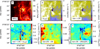 |
Fig. 12 As Fig. 11 but zooming in on the northern clump. |
| In the text | |
|
Fig. 13 Comparison of radial-velocity estimates from ideal and synthetic ngVLA observations of H13CO+(1−0). Frames a–c show, respectively, the true column density, the radial velocity from ideal observations, and the radial velocity from synthetic ngVLA observations. Frame d shows the radial velocity along the four paths (starting at the core location) indicated in frames a–c. The radial velocity from ideal observations is plotted with solid lines and the velocity from synthetic ngVLA observations with dashed lines. |
| In the text | |
|
Fig. 14 Results of PCA analysis of ideal and synthetic ngVLA observations of the 13CO and C18O lines. The quoted exponents of the scaling relation correspond to least-squares fits to the filled symbols. |
| In the text | |
|
Fig. 15 Maps of infall index ξ computed from the 3D model. Upper frames show the peak density along each LOS (frame a) and the distance (relative to the cloud centre) to that location along the LOS (frame b). The lower frames show the ξ maps for density thresholds n0 = 104 cm−3 and n0 = 106 cm−3. The dark green colour corresponds to masked areas where the maximum density along the LOS falls below the density threshold n0. |
| In the text | |
|
Fig. 16 Maps of infall index ξ towards the cores. Upper frames show maps of the peak LOS density towards the northern (frame a) and the southern (frame b) core. The lower frames show the corresponding maps of the infall index ξ, which are computed using a threshold value of n0 = 104 cm−3. |
| In the text | |
|
Fig. 17 Collapse indicators δV based on ideal C18O and 13CO observations. The upper and lower frames show, respectively, the northern and the southern clumps, for the same area as in Fig. 16. Frames a and d show δυ(proflle) that is computed from channels around the peak of the C18O spectrum. Frames b and e show the corresponding δυ (Gaussian) that is based on line parameters from Gaussian fits. For comparison, frames c and f show the skewness of the 13CO line profiles. |
| In the text | |
|
Fig. 18 Contributions of different LOS regions to a selected HCO+(1−0) spectrum. In frames a and b, the y-axis corresponds to the distance from the observer’s side of the model cloud, and the x-axis shows the radial velocity. Frame a shows the intensity of the local emission that reaches the observer and thus contributes to the observed spectrum in frame d. Frame b shows the same as the fraction of the local emission that is not absorbed by the foregrounds. The cyan contours are drawn around significant emission, to help the comparison between the frames a and b. In frame b, the observed fraction of emission is plotted only inside the contour. Frame e shows the corresponding fictitious optically thin spectrum, where all foreground absorption is ignored. The LOS variations in density (black curve) and kinetic temperature (red curve) as shown in frame c. |
| In the text | |
|
Fig. 19 Comparison of N2H+ observations with and without single-dish data. The top left frame shows the N(N2H+) column-density map that is derived from the combined ngVLA and single-dish data. The circle in the lower left corner corresponds to the 0.55″ resolution of the final map, and the circle in the lower right corner shows the 8.1″ beam of the single-dish data. The bottom left frame shows a comparison of the column-density estimates along the path that is plotted in the first frame. Results are shown for ideal observations and for ngVLA and single-dish observations when both are included in the cleaning process (“combined”) or when they are joined afterwards through feathering (“feathered”). We plot also the true column density that is obtained directly from the model cube. The right-hαnd frames show sample spectra towards the four positions marked in the first frame. The spectra from interferometric observations without combined single-dish data (“ngVLA”) are also shown. |
| In the text | |
|
Fig. 20 Column-density estimated from C18O versus 13CO (frame a) and H13CO+ versus HCO+ (frame b) line ratios, plotted against the true column density N′(H2) (accounting for the effect of density-dependent fractional abundances). Results are shown for both ideal observations and the combined ngVLA and single-dish data. The diagonal dashed line corresponds to the expected one-to-one relation. For each dataset (listed in the legends) there are four contour levels that are equidistant from close to zero up to 80% of the maximum point density. The background greyscale images correspond to the estimates calculated from ngVLA line ratios. In frame a, the estimates for optically thin C18O emission at Tex = 15 K are shown for comparison. Plots use data within 10″ of the pointing centres and a resolution of 0.7″. |
| In the text | |
|
Fig. A.1 Maps of dust emission at 250 µm (left frame) and dust colour temperature (right frame). The dashed line shows the area discussed in the main part of the paper. The data correspond to the full resolution of the cloud model (using 0.05″ pixel size for the plot). |
| In the text | |
|
Fig. B.1 Stereographic images of the high-density structures (frames a and b) and the PPV structures extracted from synthetic 13CO ngVLA observations (frames c and d). The density structures correspond to regions above n = 3 × 105cm−3 and the PPV structures to individual Gaussian components brighter than 3.5 Κ in brightness temperature. |
| In the text | |
|
Fig. B.2 Spectra for selected LOS with strong inflow motions. The first frame shows the inflow index ξ convolved to 1″ resolution. Crosses mark five locations with large ξ values, and the plots on the right show spectra for these positions (rows in decreasing order of latitude). Spectra in the first column correspond to ideal observations and the spectra in the second column to simulated ngVLA observations. Spectra are plotted for C18O (black lines), HCO+ (blue), H13CO+ (cyan), and N2H+ (dashed red lines). |
| In the text | |
|
Fig. B.3 Parameters along the LOS towards the position indicated by the northernmost cross in Fig. B.2. The first frame shows the density (black line), abundance (arbitrary normalisation and cyan line), and kinetic temperature (red line). Frame b shows same data with a zoom-in to the dashed box in frame a. The bottom frames shows the contributions of different LOS regions to the observed spectra (integrated line intensity). |
| In the text | |
|
Fig. B.4 Same as lower right frame of Fig. B.3 but splitting emission to blueshifted and redshifted parts at the mean velocity of the optically thinner species (C18O in the left and H13CO+ in the right frame). The black arrows indicate the position of the main density peak. |
| In the text | |
|
Fig. D.1 Examples of Gaussian fits towards the northern core, for simulated C18O observations (black lines) with the ngVLA Core configuration. The fits with one, two, and three Gaussian components are plotted with cyan, blue, and red lines, respectively. The spectra are taken at steps of FWHM, equal to 0.54″. |
| In the text | |
|
Fig. D.2 Test of fitting N2H+ observations containing two velocity components. The upper frames show simulated spectra (black lines) with 0.3 K observational noise and varying velocity difference δυ between the two components. Fits of a single velocity component are plotted in red for a number of noise realisations. The lower frame shows the recovered optical depth (blue line) and column density (red line) as a function of the velocity offset δυ. The shaded regions correspond to the inter-quartile range, which is computed from 128 noise realisations. The y-axis shows the ratio between the estimates and the true values. |
| In the text | |
Current usage metrics show cumulative count of Article Views (full-text article views including HTML views, PDF and ePub downloads, according to the available data) and Abstracts Views on Vision4Press platform.
Data correspond to usage on the plateform after 2015. The current usage metrics is available 48-96 hours after online publication and is updated daily on week days.
Initial download of the metrics may take a while.