| Issue |
A&A
Volume 695, March 2025
|
|
|---|---|---|
| Article Number | A18 | |
| Number of page(s) | 12 | |
| Section | Interstellar and circumstellar matter | |
| DOI | https://doi.org/10.1051/0004-6361/202452013 | |
| Published online | 28 February 2025 | |
Projection-angle effects when “observing” a turbulent magnetized collapsing molecular cloud
I. Chemistry and line transfer
1
Institute of Physics, Laboratory of Astrophysics, Ecole Polytechnique Fédérale de Lausanne (EPFL), Observatoire de Sauverny,
1290
Versoix,
Switzerland
2
Department of Physics and Astronomy, University of Western Ontario,
London,
ON
N6A 3K7,
Canada
3
Canadian Institute for Theoretical Astrophysics, University of Toronto,
60 St. George, St.,
Toronto,
ON
M5S 3H8,
Canada
4
Research School of Astronomy and Astrophysics, Australian National University,
Canberra,
ACT 2611,
Australia
5
Australian Research Council Centre of Excellence in All Sky Astrophysics (ASTRO3D),
Canberra,
ACT 2611,
Australia
★ Corresponding author; This email address is being protected from spambots. You need JavaScript enabled to view it.
Received:
27
August
2024
Accepted:
10
February
2025
Abstract
Context. Most of our knowledge regarding molecular clouds and the early stages of star formation stems from molecular spectral-line observations. However, the various chemical and radiative-transfer effects, in combination with projection effects, can lead to a distorted view of molecular clouds and complicate the interpretation of observations.
Aims. Our objective is to simultaneously study all of these effects by creating synthetic spectral-line observations based on chemo- dynamical simulations of a collapsing molecular cloud.
Methods. We performed a three-dimensional ideal magnetohydrodynamic simulation of a supercritical turbulent collapsing molecular cloud where the dynamical evolution was coupled to a nonequilibrium gas-grain chemical network consisting of 115 species, the evolution of which was governed by >1600 chemical reactions. We post-processed this simulation with a multilevel nonlocal thermodynamic equilibrium radiative-transfer code to produce synthetic position-position-velocity data cubes of the CO, HCO+, HCN, and N2H+ (J = 1 → 0) transitions under various projection angles with respect to the mean component of the magnetic field. Synthetic polarization maps are presented in a companion paper.
Results. We find that the chemical abundances of various species in our simulated cloud tend to be over-predicted in comparison to observationally derived abundances and attribute this discrepancy to the fact that the cloud collapses rapidly and therefore the various species do not have enough time to deplete onto dust grains. This suggests that our initial conditions may not correspond to the initial conditions of real molecular clouds and cores. We show that the projection angle has a notable effect on the moment maps of the species for which we produced synthetic observations. Specifically, the integrated emission and velocity dispersion of CO, HCO+ and HCN are higher when the cloud is observed “face on” compared to “edge on,” whereas column density maps exhibit an opposite trend. Finally, we show that only N2H+ is an accurate tracer of the column density of the cloud across all projection angles studied.
Key words: astrochemistry / magnetohydrodynamics (MHD) / radiative transfer / turbulence / stars: formation / ISM: clouds
© The Authors 2025
 Open Access article, published by EDP Sciences, under the terms of the Creative Commons Attribution License (https://creativecommons.org/licenses/by/4.0), which permits unrestricted use, distribution, and reproduction in any medium, provided the original work is properly cited.
This article is published in open access under the Subscribe to Open model. This email address is being protected from spambots. You need JavaScript enabled to view it. to support open access publication.
1 Introduction
In order to probe the dynamics of star-forming cores and molecular clouds, we heavily rely on spectral-line observations of various chemical tracers. Such observations are used to probe the turbulent motions within clouds and cores (Larson 1981; Heyer et al. 2009; Brunt et al. 2010; Federrath et al. 2016; Gerrard et al. 2023), estimate their angular momenta (e.g., Goodman et al. 1993; Chen et al. 2023), probe the available gas for star formation (e.g., Jones et al. 2023 and references therein), derive the kinetic temperature of the gas, probe the H2 number density of these clouds (Li & Goldsmith 2012; Tafalla et al. 2023), and derive information regarding the strength of the magnetic field (Davis 1951; Chandrasekhar & Fermi 1953; Skalidis & Tassis 2021; Bešlić et al. 2024). Yet, while observations from such tracers are routinely used, theoretical investigations are still lacking in terms of accurately and simultaneously modeling molecule formation and line-emission processes.
Three-dimensional (3D) simulations that incorporate time-dependent chemistry typically focus on a limited number of species and often involve a restricted set of chemical reactions relevant to CO chemistry and/or H2 formation (Glover et al. 2010; Micic et al. 2012; Bertram et al. 2014; Clark et al. 2019; Seifried et al. 2017; Seifried et al. 2020). Such simulations usually focus on scales of a few tens of parsecs where the formation of more complex molecular species than CO can generally be ignored. However, such simulations also lack the capacity to provide theoretical predictions regarding the expected observational characteristics of pre-stellar cores where star formation takes place, as high-density tracer molecules are not modeled. Numerical studies that focus on smaller scales and include nonequilibrium chemical modeling (e.g., Tassis et al. 2012; Keto et al. 2015; Tritsis et al. 2016, 2022, 2023) are often limited in terms of dimensionality, and therefore do not capture the full complexity of pre-stellar cores.
An alternative approach to performing chemistry “on the fly” is to post-process the dynamical simulation at a specific evolutionary stage using a time-dependent chemical model (Krumholz 2014; Godard et al. 2023; Hu et al. 2024). Such postprocessing is less computationally demanding and allows for the exploration of a larger parameter space but these methods do not reflect the significant molecular-abundance variations that can arise from different dynamical evolutionary pathways (Priestley et al. 2023). To compensate for such shortcomings, other studies have used “tracer particles” or a combination of tracer particles and nonequilibrium chemical modeling to predict the molecular abundances of various species (e.g., Navarro-Almaida et al. 2024, Priestley et al. 2024 and references therein).
Clearly, in all of the aforementioned studies, there is a trade-off between the number of species followed, and/or the methodology through which these species are modeled, and the computational cost. As such, even very detailed studies, where a large number of species are followed using an on-the-fly approach (see for instance Bovino et al. 2019), are forced to exclude more complex molecules. However, given the chaotic nature of chemical networks and the interdependence of species, excluding more complex molecules may result in inaccurate estimates of the abundances of the modeled species. In turn, such inaccuracies can propagate through the radiative-transfer calculations, undermining the overall accuracy of theoretical predictions.
In this study, we present the first results from a 3D simulation of a turbulent magnetized collapsing molecular cloud. In addition to modeling the dynamics of the cloud, we employed a nonequilibrium gas-grain chemical network to compute the abundances of 115 chemical species using an on-the-fly approach. Chemical species with up to seven atoms were modeled. We additionally post-processed this simulation with a nonlocal thermodynamic equilibrium (non-LTE) line radiative-transfer code and produced synthetic position-position-velocity (PPV) data cubes. In the present study, emphasis is placed on the qualitative aspects of our simulations and simulated observations, deferring a detailed comparison to actual observations to future research.
Our paper is organized as follows. In Sect. 2, we summarize our methods and the numerical tools used to perform the chemo-dynamical simulation and the radiative-transfer calculations. In Sect. 3.1, we discuss dynamical and chemical results, and in Sect. 3.2 we present synthetic observations of the CO, HCO+, HCN, and N2H+ (J = 1 → 0) transitions under five different projection angles with respect to the mean component of the magnetic field. In a companion paper (Tritsis et al. 2024; hereafter Paper II), we present synthetic polarization maps for the same projection angles and analyze their correlation with the simulated PPV cubes presented here. Finally, in Sect. 4, we summarize our most important results.
2 Numerical methods and setup
2.1 Numerical setup
To perform our ideal magnetohydrodynamic (MHD) chemo-dynamical simulation, we used the FLASH adaptive mesh refinement code (Fryxell et al. 2000; Dubey et al. 2008). We used a hybrid Riemann solver that combines the Roe solver (Roe 1981) for accuracy and the HLLD solver (Miyoshi & Kusano 2005) for stability, and the unsplit staggered mesh algorithm (Evans & Hawley 1988). The condition that the divergence of the magnetic field is zero, was consistently met to numerical accuracy at all times. Finally, for the Poisson equation, we used the Multigrid solver (Ricker 2008).
We used an ideal gas equation of state, assuming isothermal-ity and setting the temperature equal to T = 10 K, everywhere in the cloud. The initial number density was set equal to 500 cm−3, the magnetic field was initially along the ɀ axis and its strength was equal to 7.5 µG. As such, the mass-to-flux ratio, in units of the critical value required for the cloud to collapse (Mouschovias & Spitzer 1976), was ~2.3. The total mass of the cloud was equal to ~240 M⊙.
The dimensions of the cloud were equal to 2 pc in each direction. We used a 643 grid with two levels of refinement, such that the resolution of our smallest cell is ~ 8 × 10⁻³ pc. We used open boundary conditions in all dimensions. We refined our grid using a modified second derivative criterion of the density (Löhner 1987) and have verified that the Truelove condition (Truelove et al. 1997) was consistently met throughout the simulation. We followed the evolution of the cloud up to a “central” number density of 105 cm−3. Continuing our calculations beyond this point was overly computationally expensive. For reference, more than 2.5 million CPU hours were required to perform this simulation.
2.2 Turbulent initial conditions
We initialized a turbulent velocity field with zero mean momentum, which was generated with the public code TurbGen (Federrath et al. 2022), based on the methods described in Federrath et al. (2010). The turbulent velocity field was constructed in Fourier space (k-space), with a power-law velocity (υ) spectrum dυ2/dk ∝ k−2 in the wavenumber range 2 ≤ k ≤ 20, where k = 2π/L and L was the size of the computational domain. We generated a natural mixture of modes for the velocity field, with 2/3 of the power in solenoidal modes and 1/3 power in compressible modes, by setting ζ = 0.5 in TurbGen (see Eqs. (6–9) in Federrath et al. 2010). The standard deviation of the field was set to συ = 0.554 km/s, and with the given sound speed of cs = 0.18 km/s, this initializes a turbulent velocity field with a sonic Mach number of ℳ = συ/cs ~ 3, broadly consistent with the velocity dispersion – size relation observed in Milky Way clouds (Larson 1981; Falgarone et al. 1992; Heyer & Brunt 2004; Roman-Duval et al. 2011). This choice of initial turbulent velocity field approximates the typical turbulent conditions observed in pre-stellar clouds and cores.
2.3 Chemical modeling
The inclusion of a chemical network in dynamical simulations is imperative if we wish to have realistic chemical conditions. Having realistic chemical conditions is in turn crucial for radiative-transfer post-processing and ultimately for performing a one-to-one comparison to real observations. Here, we used the same chemical network as in Tritsis et al. (2022) and Tritsis et al. (2023) (see also Tritsis et al. 2016) consisting of 115 species, 48 out of which were ions and 37 were ice-mantle species. At each grid point and for every timestep, the evolution of these species was governed by ~1650 chemical reactions. These reactions encompassed a range of processes, including freeze-out, thermal desorption, photodissociation, photoionization, cosmic-ray ionization, cosmic-ray induced photo processes, and grain-surface chemical reactions. Reaction rates were taken from the UMIST database (McElroy et al. 2013). In a future work, we plan to update our chemical network to incorporate the latest reaction rates provided by Millar et al. (2024). The initial elemental abundances can be found in Table 1 of Tritsis et al. (2022).
The visual extinction that enters in the determination of the reaction rates of photo-related processes was calculated using an on-the-fly approach based on the six-ray approximation. Following Glover & Clark (2012b) the “3D”  is given by
![Mathematical equation: $A_\v ^{3D} = - {1 \over f}log\left[ {{1 \over 6}\mathop \sum \limits_1^6 {e^{ - f{A_{\v ,i}}}}} \right] + C,$](/articles/aa/full_html/2025/03/aa52013-24/aa52013-24-eq2.png) (1)
(1)
where Aυ,i is the visual extinction along each direction in each of the principal axes of our numerical grid. The inclusion of the factor f was based on the scaling of the photodissociation rate with visual extinction, as  . Here, we adopted f = 2.3 which represents an average scaling factor of all species in the chemical network. To convert between column density
  and visual extinction Aυ,i we followed Pineda et al. (2010) and used
  cm−2 mag−1. Given that the simulation presented is intended to represent a subregion of a molecular cloud, a constant offset C was also used in Eq. (1). The addition of an offset in Eq. (1) also ensures that there are no issues at the boundaries of our simulation, where the computed value of
  would otherwise be ≪ 1. Here, we adopted a value of C = 1.5 mag (see for instance Table 1 from Kainulainen et al. 2011 for an estimate of the average visual extinction in nearby molecular clouds).
A similar expression as Eq. (1) was also used for the calculation of the cosmic-ray ionization rate. To convert between the column density and the cosmic-ray ionization rate we used (Umebayashi 1983)
 (2)
(2)
where ζ0 = 1.3 × 10⁻¹⁷ s−1 is the “standard” cosmic-ray ionization rate (Caselli et al. 1998), and  is the mass column density. However, given the range of column densities that we followed here (<1023cm−2; see Fig. 1 in Paper II), the exponential factor on the right-hand side of Eq. (2) was always very close to unity, and only very small deviations (≪ 1%) from the standard value were found.
2.4 Line radiative-transfer simulations
To create synthetic spectral-line observations we used the non-LTE multilevel radiative-transfer code PYRATE (Tritsis et al. 2018; Tritsis & Kylafis 2024). PYRATE uses a ray-tracing approach to solve the radiative-transfer problem with the level populations calculated using a Λ-iteration. While doing so, we took into account that photons emitted from one region of the cloud would interact with another region, provided that the relative velocity between the two regions is less than the thermal linewidth. Consequently, this approach allowed us to account for the coupling of the level populations over the entire cloud (see also the discussion in Appendix C in Tritsis & Kylafis 2024). To save computational time, however, we neglected the hyperfine structure of molecules, where relevant.
All of our radiative-transfer calculations were performed under non-LTE conditions, assuming five rotational levels and we post-processed our simulation at a resolution of 1283 grid cells. The contribution from the Cosmic Microwave Background radiation was taken into account when computing the level populations. Collisional and Einstein coefficients were taken from the LAMBDA database (Schöier et al. 2005). For all of our radiative-transfer calculations we assumed a spectral resolution of 0.05 km s−1 and 64 points in frequency space. Finally, intensities were converted to brightness-temperature units and noise was added to the spectra such that the signal-to-noise ratio in the center of the cloud was equal to 20 in all modeled PPV data cubes.
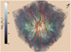 |
Fig. 1 Isometric 3D view of the H2 number-density distribution (color-coded isosurfaces) within the simulated cloud. Red lines show the magnetic field lines and green vectors show the velocity field in the cloud. |
3 Results
Throughout this manuscript, we use x, y, ɀ, to denote our axes when we show results associated with 3D quantities (e.g., number density), and ξ and η for results associated with synthetic observations (i.e., moment maps from our synthetic PPV cubes), including when the line of sight (LOS) coincides with one of the principal axes of the grid. In all images associated with synthetic observations, we annotate the azimuthal and polar angles (θ and ϕ, respectively) under which the cloud is “observed” such that there is no confusion regarding the projection angle. A schematic illustration of the angles and definitions associated with synthetic observations can be found in Fig. 1 of Paper II.
3.1 Chemo-dynamical results
In Fig. 1, we present a 3D isometric view of our simulated cloud when the central number density is ~ 105 cm−3. The magnetic field is depicted using red lines and the green vectors show the velocity field. The cloud exhibits a complex structure, but despite the fact that it is supercritical and super-Alfvénic, it has still contracted along the magnetic-field lines (i.e., along the ɀ axis). Consequently, a flattened structure with “mean density” of ~104 cm−3 has formed with its short axis oriented parallel to the magnetic field. That is, the structure itself lies approximately in the x-y plane. For reference, the orientation of the coordinate axes is indicated in the top right corner of Fig. 1.
3.1.1 Qualitative features in molecular abundances
In Fig. 2, we present molecular-abundance slices along the x axis. The slices are averaged within 0.05 pc and centered at the location of the maximum H2 number density. The calculated molecular abundances exhibit certain general qualitative trends, observed in molecular clouds and pre-stellar cores. The CO abundance (upper row, middle panel) decreases by almost an order of magnitude from the outskirts of the cloud to the location of maximum number density where it is depleted onto dust grains. HCO+ (upper row, right panel) is significantly more concentrated toward the densest regions of the cloud but it is still abundant at H2 number densities of 103 cm−3. Similarly, HCN (middle row, left panel) also appears to be significantly abundant even at the lower-density regions of the cloud of ~ 103 cm−3 (e.g., Pety et al. 2017; Kauffmann et al. 2017; Tafalla et al. 2021; Jones et al. 2023). In terms of the “traditional” high-density tracers, N2H+ is visibly more extended than NH3 (middle row, right and middle panels, respectively), as observations of dense cores also suggest (e.g., Tafalla et al. 2002; Chitsazzadeh et al. 2014). We note here that such differences in the abundance distributions between these two species could potentially account for the fact that the N2H+ spectra have been found to have larger linewidths than those of NH3 (Pineda et al. 2021). The abundance distributions of HC3N and H2CO (bottom row, left and middle panels, respectively) also seem to be in line with observations in terms of the fact that they peak off center in comparison to the H2 number density (Tafalla et al. 2006).
An important trend that can be observed throughout Fig. 2 is that the abundance distributions of various species appear to be significantly affected by (and often follow) the 3D visual extinction (colored contours in Fig. 2) which peaks off center in comparison to the H2 number density. In 3D space, as well as in the slices presented in Fig. 2, the distance between the density and visual extinction peaks is ~0.22 pc. Apart from the effect of depletion, this trend may also be a potential reason why certain species peak off center with respect to the continuum peak.
Another notable feature in Fig. 2 is that the small “filaments” evident in the H2 density distribution (upper left panel) are neither evident in the visual extinction (colored contours) nor in the species. The differences in the filamentary structures seen in the H2 density and extinction map arise from the averaging process inherent in the six-ray approximation used to calculate  (Eq. (1)). While the H2 density reflects sharp variations caused by the turbulent flow,
  is influenced by contributions from all six directions, which effectively “smooths out” these sharp changes. Therefore, this smoothening of the small filamentary structures occurs because
  is not localized but rather determined by the surrounding structure from multiple directions.
This smoothing effect of  also indirectly propagates to the molecular-abundance distributions. However, the fact that other molecular species exhibit different or smoother abundance distributions, lacking the small-scale filaments observed in the H2 number density, is not solely due to photo-related processes. These differences arise from the complex interdependence between species in the chemical network, combined with varying timescales and the chemical history of the cloud. In the cloud center, for the time shown in Fig. 2, and for the chemical history of this specific simulated cloud, HCN is primarily produced through reactions involving HCNH+ and electrons, and destroyed by reactions with H2CO+. CO is produced via reactions involving HCO+ and electrons, and destroyed by freezing onto dust grains or reacting with H+. Only N2H+ is more closely tied to the H2 density, since H2 is directly involved in its production, although the dominant production mechanism still involves reactions between
  and N2. For the time shown in Fig. 2, all of these reactions occur on much shorter timescales than the dynamical timescale of the cloud, meaning that chemistry can, in principle, respond rapidly to the formation of the small filaments observed in the H2 density distribution. However, this is not the case as the formation and destruction of these species is not typically directly tied to the H2 density, and even when it is (as in the production of N2H+), the other reactant (e.g.,
  in the case of N2H+) must also reflect to some extent the same features.
 |
Fig. 2 Averaged slices (within 0.05 pc) along the x axis, centered at the location of the maximum number density in the cloud, showing the spatial distribution of various molecules. In the upper left panel, we show the H2 number density, and in the rest of the panels we show the abundances of various, commonly observed species. The dotted red, dash yellow, dash-dotted blue, and solid violet contours represent 30, 50, 70, and 90% of the maximum 3D visual extinction within the cloud, respectively. |
3.1.2 Comparison of modeled and observed abundances
From a quantitative standpoint, the picture is far less clear. Specifically, the abundances of some species are over-predicted compared to what observations suggest. Bergin et al. (2002) and Lin et al. (2020) both estimated the N2H+ abundance to be ~3 × 10⁻¹¹ in the pre-stellar cores L1512 and B68, respectively. Such values are ~1 order of magnitude lower than what is calculated in our simulation. A similar argument can be made for the abundances of HCO+ (see for instance the abundance estimates in Table 9 of Pety et al. 2017). Tafalla et al. (2006) estimated the fractional abundance of this molecule to be ~3 × 10⁻⁹ and ~1.5 × 10⁻⁹ in the pre-stellar cores L1498 and L1517B, respectively. Such values are again lower by a factor of ~5 than those calculated in our model. For the same cores, the abundance of H2CO is also estimated to be ~one order of magnitude lower than the predictions of the model, while the abundance of HC3N is in agreement with observational estimates (see also the discussion below). In line with this trend, the observational estimates for the abundance of CH3CN in the pre-stellar cores L1544, L1498 and L1517B are also lower by a factor of ~5–10 compared to model predictions (Megías et al. 2023).
Some of these differences may arise due to the specific details of the chemical network employed. Variations in reaction rates across chemical databases, and differences in the number of reactions or species considered, can result in abundance variations of up to a factor of ~5 for certain molecules (e.g., Wakelam et al. 2012, Fig. 1). However, in our case, we observe differences often spanning orders of magnitude between the abundances of several molecules in our simulated cloud and those observed. This indicates that the issue likely lies not in the calculation of abundances but rather in the initial conditions of the simulated cloud, which may not accurately represent real clouds. A slower cloud collapse, resulting from different initial conditions, could potentially reduce these differences. For instance, an initially stronger magnetic field such that the cloud was subcritical, and/or a higher initial sonic Mach number could provide additional support against gravity. This would in turn allow chemistry more time to evolve at lower densities and visual extinctions.
The fundamental role of initial conditions in shaping the chemical evolution of molecular clouds becomes evident if we compare the abundances of CO and HCO+ in our modeled cloud with those obtained from subcritical simulations, where collapse occurs more slowly. For instance, in their 2D subcritical models, Tritsis et al. (2022) found CO and HCO+ abundances that were one to two orders of magnitude lower than those calculated here for the same central density (see their Figure 10). This is to be expected, as the cloud presented here reaches this evolutionary stage very rapidly (i.e., within ~1.8 Myrs) and, as a result, these species do not have enough time to deplete onto dust grains. Specifically, the depletion timescale of CO in our chemical network at a density of 104 cm−3 is 0.56 Myrs (see also Bergin & Tafalla 2007). Comparing the depletion timescale with the free-fall time at the same density, we find that τdepl/tff = 1.7. In contrast, initially subcritical modeled clouds can spend a significant portion of their lifetime (4–8 Myr) at densities of 103–104 cm−3 (see Figure 1 in Tritsis et al. 2023). At these densities, the depletion timescale is shorter by a factor of 2–10 compared to the dynamical timescale, which, in this case, is the ambipolar-diffusion timescale. A similar trend, where the abundances of various species were higher in supercritical models compared to subcritical ones was also observed in the chemo-dynamical simulations by Tassis et al. (2012).
While in most instances the abundances from the model are larger than observational estimates, there are some cores and clouds where the calculated abundances are in fair agreement with observations or even lower. For example, the HC3N abundance calculated in Lupus starless cores is in very good agreement with model predictions (Wu et al. 2019). In relative terms, the abundance of HC3N over that of NH3 also appears to be in rough agreement with observations (Xie et al. 2021), albeit the uncertainties span ~two orders of magnitude and therefore no robust conclusions can be drawn. The N2H+ abundance in the pre-stellar cores L1498 and L1517B (Tafalla et al. 2006) is also in very good agreement with the predictions of the model, while for the same cores, the estimated NH3 abundance is larger than what is calculated from our nonequilibrium chemical model.
From the above discussion it becomes clear that there are order-of-magnitude uncertainties when performing a comparison between model predictions of molecular abundances and observational estimates. Additionally, the results from our model might agree with observations of some cores and clouds and disagree with others. As a result, no definitive conclusion can be drawn using this single model, albeit the present comparison suggests that the initial conditions of our simulated cloud may not accurately represent real clouds. Therefore, a careful dedicated study is required with an extensive literature review of observational abundance estimates of many molecular species over a range of H2 densities. A statistical comparison with the results from many different chemo-dynamical models with different initial and physical conditions can then reveal invaluable information regarding the histories of these clouds. In the future, we will revisit this issue with a broader suite of simulations, including subcritical models under nonideal MHD conditions.
3.2 Synthetic line-emission observations
In Fig. 3, we show moment maps from simulated PPV cubes of the CO J = 1 → 0 transition. Moment maps from simulated PPV cubes of the HCO+, HCN, and N2H+ J = 1 → 0 transitions are shown in Figs. A.1, A.2, and A.3, respectively. In the left column we show the velocity-integrated emission maps, in the middle column we show the first-moment maps, and finally in the right column we show the second moment maps. Different rows correspond to simulated PPV cubes under different projection angles starting from “face on” (ϕ = 0°; upper row) to “edge on” (ϕ = 90°; bottom row). The colored contours overplotted on top of the zeroth moment maps for each projection angle correspond to the column density with contour levels set equal to 30, 50, 70, and 90 % of the maximum column density in each specific projection angle (dotted red, dash yellow, dash-dotted blue and solid violet lines, respectively). Column density maps for the same projection angles are presented in Paper II.
The red ellipses in the right column of Fig. 3 show different regions selected to extract mean values of the zeroth and second moment maps as a function of the projection angle. As the polar angle increases from 0° to 90°, the shape of these regions transitions from a circle to an ellipse with progressively greater eccentricity to account for the observed morphology of the cloud. Importantly, we ensured that the area of these regions remains constant across all projection angles. The size of these regions was determined based on two criteria. First, a physical criterion, as our primary interest lies in the inner parts of the cloud, where the emission from the rest of the simulated species is also concentrated (i.e., see Fig. A.3). Secondly, a statistical criterion, as the zeroth moment map values within these regions exhibit a roughly Gaussian distribution (for most projection angles and molecules). We verified that changing the size and/or the shape of these regions does not qualitatively impact our results. Our results for the mean values of the zeroth and second moment maps are shown in the upper and lower Fig. 4, respectively. With the black, red, cyan and magenta lines we show our results for CO, HCO+, HCN, and N2H+, respectively. The shaded regions in each panel show the 16th and 84th percentiles of the respective distributions inside the red regions in the left column of Fig. 3.
As evident from Fig. 3, the CO emission does not probe the densest parts of the cloud and systematically peaks off center in comparison to the column-density peaks. While this statement holds true for all projection angles, the effect is more prominent for polar angles close to 90° where two quasi-parallel (to each other and to the column-density filament) elongated structures are observed. Additionally, the average integrated emission systematically decreases with an increasing value of the polar angle by approximately ~30–50% from face on to edge on. This trend is more clearly evident in the upper panel of Fig. 4 (black line and shaded region). Similarly, this trend in mean integrated intensity is observed in the zeroth moment maps of HCN and HCO+ (see Figs. A.1–A.2 and red and cyan lines in Fig. 4).
With regards to the qualitative features in the zeroth moment maps, HCN and HCO+ exhibit a more complex behavior. For large values of the polar angle, both molecules are fair tracers of the column density, albeit both species peak off center in comparison to the column density peak. For such projection angles, HCO+ exhibits a more rapid decline than HCN in integrated intensity towards the outskirts of the cloud. For smaller values of the polar angle, both species trace the column density significantly better than CO. However, HCN performs significantly better in the highest column density regions (column density contours >50%). In terms of mean values within the selected regions (red ellipses in Fig. 3), HCO+ declines faster as a function of the projection angle than HCN (see red and cyan lines in the upper panel of Fig. 4).
Among all species for which we have produced synthetic PPV data cubes, only N2H+ is a good tracer of the H2 column density across all projection angles (left column in Fig. A.3). We note, however, that this does not necessarily imply that N2H+ also traces the H2 number-density peak. Specifically, due to the complex 3D structure of the cloud, the location of the column-density peak does not exactly coincide with the location of the number-density peak. Additionally, N2H+ is the only species for which the integrated emission does not systematically decrease as a function of the projection angle (from face on to edge on). In contrast, by comparing the upper left and lower left panels of Fig. A.3, we observe an increase in integrated emission by ~20% in the higher column density contours (>70%; dash-dotted blue lines), while the average value in the selected red regions shown in the right column of Fig. 3 remains roughly constant with projection angle (see magenta line in the upper panel of Fig. 4).
A similar pattern to the zeroth moment maps is also seen in the second moment maps of our simulated PPV cubes (see right columns in Figs. 3, A.1–A.3 and the lower panel in Fig. 4). That is, the dispersion of the LOS velocity is ~20–30% higher when the cloud is observed face on in comparison to when it is observed edge on. The same trend is evident in the synthetic PPV cubes of all simulated species. This is due to the fact that, even though the modeled cloud is supercritical, it still primarily collapses along magnetic field lines. As such, the velocity dispersion observed for small polar angles is primarily due to gravitational collapse. Interestingly enough however, these systematic motions along magnetic field lines are not particularly evident in the first moment maps of intermediate projection angles (ϕ = 22.5°, 45° and 67.5° shown in the second, third and fourth rows of Fig. 3, A.1–A.3, respectively), although a global gradient is observed. Instead, the first moment maps are primarily dominated by the turbulent motions within the cloud and exhibit both red and blue-shifted motions above and below the “midplane” of the cloud (η = 0 pc).
Additionally, the velocity dispersion derived from HCN synthetic observations is somewhat higher than that derived from HCO+ by ~0.03–0.05 km s−1 for polar angles close to face on. We note that, since our simulation was performed assuming ideal MHD conditions, if HCO+ and HCN probed the same gas, the derived LOS velocity dispersion should be the same. This offset is also not constant with respect to the projection angle and when the cloud is seen edge on the derived velocity dispersion from HCO+ is slightly higher than HCN. While such differences in the derived LOS velocity dispersion might seem insignificant, they are a significant fraction of the expected ion-neutral drift velocity for central number densities of 105 cm−3. Given that these two species also probe different parts of the cloud (see discussion above) corroborate the findings by Tritsis et al. (2023) that these two species cannot be used to probe ambipolar diffusion in molecular clouds.
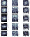 |
Fig. 3 Moment maps from the CO (J = 1 → 0) transition from our chemo-dynamical simulation under different projection angles. In the left, middle and left columns we show the zeroth, first and second moment maps, respectively. In the upper row the mean component of the magnetic field is along the LOS, whereas in the bottom row the mean magnetic field lies in the plane of the sky. Intermediate angles are shown in the second, third and fourth rows (the azimuthal and polar angles are indicated in the upper left corners of the zeroth moment maps). The red dotted, yellow dash, blue dash-dotted, and solid violet contours represent 30, 50, 70, and 90% of the maximum column density, respectively. The red ellipses in the right column show the region used to extract average values as a function of the projection angle (see text and Fig. 4). |
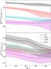 |
Fig. 4 Dependence of the average of the zeroth and second moment maps (upper and lower panels, respectively) on the projection angle for each of the species for which we have produced synthetic observations. Averages are computed within the red ellipses shown in the rightcolumn of Fig. 3. Shaded regions show the 16th and 84th percentiles of the distributions of values within the ellipses shown in the right column of Fig. 3. For all species, we observe a decrease in the derived velocity dispersion with increasing polar angle. The same trend is true for the velocity-integrated emission, apart from N2H+, for which the average of the zeroth-moment maps remains roughly constant. |
3.3 Caveats
A key assumption made throughout this study is that the gas is isothermal. Departures from isothermality can significantly influence the abundances of species in our chemical network, as most reaction rates are temperature dependent, and can also impact the observed line profiles. Line profiles will be affected by both temperature-driven changes in collisional excitation and through variations in the optical depth. For instance, an increase in temperature will increase the thermal linewidth, causing more cells to fall within one thermal linewidth away from each other (see Sect. 2.4), which will, in turn, lead to a higher cumulative optical depth along a given LOS.
Ammonia observations (e.g., Lemme et al. 1996; Seo et al. 2015; Friesen et al. 2017) have established that, at the scales of cores, the temperature remains nearly constant, with only small variations on the order of 2–3 K. Additionally, theoretical work (e.g., Goldsmith 2001; Galli et al. 2002) has demonstrated that variations in the abundances of the main coolants, such as C+ and CO (e.g., Goldsmith & Langer 1978), at high densities (≳104 cm−3) do not significantly affect the temperature. This is because gas-dust coupling ensures that any reduction in gas-phase cooling is balanced by energy exchange between gas and dust, and because molecular cooling transitions are often optically thick. Finally, chemo-dynamical simulations including heating and cooling processes (e.g., Glover et al. 2010; Glover & Clark 2012a) have shown that for visual extinctions ≳4 mag, the gas is nearly isothermal. For reference, the maximum visual extinction in our simulation is ~14 mag. At lower densities ≲ 103 cm−3, we should expect temperature variations of the factor of 2-3, as CO observations of molecular clouds also suggest (e.g., Goldsmith et al. 2008).
Given the above discussion, we do not expect any realistic temperature variations to significantly impact our results on molecular abundances, particularly in the central regions of the cloud (≳104 cm−3), which are the focus of the present study. Furthermore, in the lower-density outskirts, the abundance of CO does not exhibit substantial variation except at the very edges of the cloud (see Fig. 2). This suggests that temperature variations in these regions should also remain limited, although this conclusion is constrained by the absence of explicit heating and cooling processes in our modeling.
Regarding the line profiles, the flattened structure of our modeled cloud, implies that any temperature increases in the outskirts are likely to be more pronounced along the ɀ axis. Such variations would preferentially enhance the values in the zeroth and second moment maps when the cloud is viewed face on compared to edge on, due to the broader linewidths and increased excitation. In the edge-on case, temperature variations would primarily affect the gradients of the zeroth and second moment maps from the center to the outskirts1. As such, the observed trends in the moment maps discussed here, should be robust and would likely be strengthened rather than diminished by any realistic temperature variations.
4 Summary and conclusions
We have presented first results from a 3D ideal MHD turbulent chemo-dynamical simulation of a collapsing molecular cloud, where we simultaneously followed the evolution of 115 chemical species. By post-processing this simulation with a non-LTE radiative-transfer code we produced line-emission synthetic observations under various projection angles, including on and off-axis projections. Synthetic dust-polarization observations were also created for the same projection angles and are presented in a companion paper.
We find that the abundance distributions of various species in our chemo-dynamical simulation can qualitatively explain certain features observed in molecular-emission maps. Specifically, we find evidence for CO depletion in the densest regions of the cloud, that the HCN abundance remains high (~6.5 × 10⁻¹⁰) even in lower-density regions (~103 cm−3), and that NH3 is more peaked (in relation to the H2 number density) than N2H+. However, quantitatively, there is a tendency for the abundances of most species in our simulation to be overpredicted in comparison to most observational estimates. We attribute this trend to the fact that the cloud collapses rapidly and, as a result, these species do not have enough time to deplete onto dust grains. Our results hint that the initial conditions used in this specific model might not be entirely representative of real molecular clouds and cores.
From our synthetic observations we found that the projection angle has a notable effect on the observed properties of the cloud. For three out of four simulated species (CO, HCO+, and HCN), there is a decrease in the values of their zeroth moment maps (by ~30–50%) as the polar angle increases. Only for N2H+ the zeroth moment map remains roughly constant (with even a slight increase in the very central regions) from face on to edge on. For all species, the velocity dispersion measured, is higher when the cloud is observed face on rather than when it is seen edge on. This is to be expected, as the cloud is primarily collapsing along magnetic-field lines and we are therefore observing the effect of gravity. However, such motions are not easily distinguishable in the first moment maps of the simulated species as turbulence significant affects their overall structure.
In Paper II, we show that column density maps exhibit an opposite trend compared to the zeroth and second moment maps with respect to the projection angle. That is, the column density is higher when the cloud is seen edge on compared to when it is seen face on. Such complications, related to the projection angle, can affect observational estimates of various quantities, including those for the magnetic field strength (calculated using the Davis-Chandrasekhar-Fermi method and its variants), since all three input quantities, δυ, δθ and  , are affected by the inclination angle. Additionally, the H2 column density and the zeroth moment maps of molecular emission are inversely related to the projection angle. That is, the values of H2 column density increase with an increasing polar angle whereas the values in the zeroth moment maps decrease. Therefore, the slope in the relation between integrated molecular emission and column density, as examined in recent observational studies (Tafalla et al. 2023), should also be affected by the projection angle.
Acknowledgements
We are grateful to K. Tassis for stimulating discussions. We are also grateful to the referee for their constructive feedback and suggestions which helped enhance the clarity and quality of our manuscript. A. Tritsis acknowledges support by the Ambizione grant no. PZ00P2_202199 of the Swiss National Science Foundation (SNSF). S. Basu was supported by a Discovery grant from NSERC. C. Federrath acknowledges funding provided by the Australian Research Council (Discovery Projects DP230102280 and DP250101526). The software used in this work was in part developed by the DOE NNSA-ASC OASCR Flash Center at the University of Chicago. This research was enabled in part by support provided by SHARCNET (Shared Hierarchical Academic Research Computing Network) and Compute/Calcul Canada and the Digital Research Alliance of Canada. We further acknowledge high-performance computing resources provided by the Leibniz Rechenzentrum and the Gauss Centre for Supercomputing (grants pr32lo, pr48pi and GCS Large-scale project 10391), the Australian National Computational Infrastructure (grant ek9) and the Pawsey Supercomputing Centre (project pawsey0810) in the framework of the National Computational Merit Allocation Scheme and the ANU Merit Allocation Scheme. We also acknowledge use of the following software: MATPLOTLIB (Hunter 2007), NUMPY (Harris et al. 2020), SCIPY (Virtanen et al. 2020) and the YT analysis toolkit (Turk et al. 2011).
Appendix A Dense-gas tracers
In this Appendix we present moment maps for additional molecular species. Specifically, we have performed non-LTE radiative-transfer calculations for HCO+, HCN and N2H+. In the interest of saving computational time, we have ignored the hyperfine structure for our N2H+ radiative-transfer simulations. The corresponding moment maps are shown in Figs. A.1, A.2, A.3.
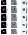 |
Fig. A.3 Same as Fig. 3 but for the N2H+ (J = 1 → 0) transition. In contrast to the other species studied here, N2H+ is a good tracer of the column density for most projection angles. |
References
- Bergin, E. A., & Tafalla, M. 2007, ARA&A, 45, 339 [Google Scholar]
- Bergin, E. A., Alves, J., Huard, T., et al. 2002, ApJ, 570, L101 [NASA ADS] [CrossRef] [Google Scholar]
- Bertram, E., Shetty, R., Glover, S. C. O., et al. 2014, MNRAS, 440, 465 [CrossRef] [Google Scholar]
- Bešlić, I., Coudé, S., Lis, D. C., et al. 2024, A&A, 684, A212 [NASA ADS] [CrossRef] [EDP Sciences] [Google Scholar]
- Bovino, S., Ferrada-Chamorro, S., Lupi, A., et al. 2019, ApJ, 887, 224 [NASA ADS] [CrossRef] [Google Scholar]
- Brunt, C. M., Federrath, C., & Price, D. J. 2010, MNRAS, 403, 1507 [Google Scholar]
- Caselli, P., Walmsley, C. M., Terzieva, R., et al. 1998, ApJ, 499, 234 [NASA ADS] [CrossRef] [Google Scholar]
- Chandrasekhar, S., & Fermi, E. 1953, ApJ, 118, 113 [Google Scholar]
- Chitsazzadeh, S., Di Francesco, J., Schnee, S., et al. 2014, ApJ, 790, 129 [NASA ADS] [CrossRef] [Google Scholar]
- Chen, C.-Y., Friesen, R., Li, J., et al. 2024, MNRAS, 527, 10279 [Google Scholar]
- Clark, P. C., Glover, S. C. O., Ragan, S. E., et al. 2019, MNRAS, 486, 4622 [CrossRef] [Google Scholar]
- Davis, L. 1951, Phys. Rev., 81, 890 [Google Scholar]
- Dubey, A., Fisher, R., Graziani, C., et al. 2008, Numer. Model. Space Plasma Flows, 385, 145 [NASA ADS] [Google Scholar]
- Evans, C. R., & Hawley, J. F. 1988, ApJ, 332, 659 [Google Scholar]
- Falgarone, E., & Puget, J.-L. 1995, A&A, 293, 840 [NASA ADS] [Google Scholar]
- Falgarone, E., Puget, J.-L., & Perault, M. 1992, A&A, 257, 715 [NASA ADS] [Google Scholar]
- Federrath, C., Roman-Duval, J., Klessen, R. S., et al. 2010, A&A, 512, A81 [NASA ADS] [CrossRef] [EDP Sciences] [Google Scholar]
- Federrath, C., Rathborne, J. M., Longmore, S. N., et al. 2016, ApJ, 832, 143 [NASA ADS] [CrossRef] [Google Scholar]
- Federrath, C., Roman-Duval, J., Klessen, R. S., et al. 2022, Astrophysics Source Code Library [record ascl:2204.001] [Google Scholar]
- Friesen, R. K., Pineda, J. E., co-PIs, et al. 2017, ApJ, 843, 63 [NASA ADS] [CrossRef] [Google Scholar]
- Fryxell, B., Olson, K., Ricker, P., et al. 2000, ApJS, 131, 273 [Google Scholar]
- Galli, D., Walmsley, M., & Gonçalves, J. 2002, A&A, 394, 275 [NASA ADS] [CrossRef] [EDP Sciences] [Google Scholar]
- Gerrard, I. A., Federrath, C., Pingel, N. M., et al. 2023, MNRAS, 526, 982 [NASA ADS] [CrossRef] [Google Scholar]
- Glover, S. C. O., & Clark, P. C., 2012a, MNRAS, 421, 9 [NASA ADS] [Google Scholar]
- Glover, S. C. O., & Clark, P. C. 2012b, MNRAS, 421, 116 [NASA ADS] [Google Scholar]
- Glover, S. C. O., Federrath, C., Mac Low, M.-M., et al. 2010, MNRAS, 404, 2 [Google Scholar]
- Godard, B., Pineau des Forêts, G., Hennebelle, P., et al. 2023, A&A, 669, A74 [NASA ADS] [CrossRef] [EDP Sciences] [Google Scholar]
- Goldsmith, P. F. 2001, ApJ, 557, 736 [Google Scholar]
- Goldsmith, P. F., & Langer, W. D. 1978, ApJ, 222, 881 [Google Scholar]
- Goldsmith, P. F., Heyer, M., Narayanan, G., et al. 2008, ApJ, 680, 428 [Google Scholar]
- Goodman, A. A., Benson, P. J., Fuller, G. A., et al. 1993, ApJ, 406, 528 [CrossRef] [Google Scholar]
- Harris, C. R., Millman, K. J., van der Walt, S. J. et al. 2020, Nature, 585, 357 [NASA ADS] [CrossRef] [Google Scholar]
- Heyer, M. H., & Brunt, C. M. 2004, ApJ, 615, L45 [NASA ADS] [CrossRef] [Google Scholar]
- Heyer, M., Krawczyk, C., Duval, J., et al. 2009, ApJ, 699, 1092 [Google Scholar]
- Hu, Z., Wibking, B. D., Krumholz, M. R., & Federrath, C. 2024, MNRAS, 534, 2426 [NASA ADS] [CrossRef] [Google Scholar]
- Hunter, J. D. 2007, Comput. Sci. Eng., 9, 90 [NASA ADS] [CrossRef] [Google Scholar]
- Jones, G. H., Clark, P. C., Glover, S. C. O., et al. 2023, MNRAS, 520, 1005 [NASA ADS] [CrossRef] [Google Scholar]
- Kainulainen, J., Beuther, H., Banerjee, R., et al. 2011, A&A, 530, A64 [NASA ADS] [CrossRef] [EDP Sciences] [Google Scholar]
- Kauffmann, J., Goldsmith, P. F., Melnick, G., et al. 2017, A&A, 605, L5 [NASA ADS] [CrossRef] [EDP Sciences] [Google Scholar]
- Keto, E., Caselli, P., & Rawlings, J. 2015, MNRAS, 446, 3731 [NASA ADS] [CrossRef] [Google Scholar]
- Krumholz, M. R. 2014, MNRAS, 437, 1662 [NASA ADS] [CrossRef] [Google Scholar]
- Larson, R. B. 1981, MNRAS, 194, 809 [Google Scholar]
- Le Besnerais, G., & Champagnat, F. 2005, IEEE Int. Conf. Image Process., 1, I [Google Scholar]
- Lemme, C., Wilson, T. L., Tieftrunk, A. R., et al. 1996, A&A, 312, 585 [NASA ADS] [Google Scholar]
- Li, D., & Goldsmith, P. F. 2012, ApJ, 756, 12 [NASA ADS] [CrossRef] [Google Scholar]
- Lin, S.-J., Pagani, L., Lai, S.-P., et al. 2020, A&A, 635, A188 [NASA ADS] [CrossRef] [EDP Sciences] [Google Scholar]
- Löhner, R. 1987, Comp. Meth. App. Mech. Eng., 61, 323 [CrossRef] [Google Scholar]
- McElroy, D., Walsh, C., Markwick, A. J., et al. 2013, A&A, 550, A36 [NASA ADS] [CrossRef] [EDP Sciences] [Google Scholar]
- Megías, A., Jiménez-Serra, I., Martín-Pintado, J., et al. 2023, MNRAS, 519, 1601 [Google Scholar]
- Micic, M., Glover, S. C. O., Federrath, C., et al. 2012, MNRAS, 421, 2531 [NASA ADS] [CrossRef] [Google Scholar]
- Millar, T. J., Walsh, C., Van de Sande, M., et al. 2024, A&A, 682, A109 [NASA ADS] [CrossRef] [EDP Sciences] [Google Scholar]
- Miyoshi, T., & Kusano, K. 2005, J. Computat. Phys., 208, 315 [NASA ADS] [CrossRef] [Google Scholar]
- Mouschovias, T. C., & Spitzer, L. 1976, ApJ, 210, 326 [NASA ADS] [CrossRef] [Google Scholar]
- Navarro-Almaida, D., Lebreuilly, U., Hennebelle, P., et al. 2024, A&A, 685, A112 [NASA ADS] [CrossRef] [EDP Sciences] [Google Scholar]
- Pety, J., Guzmán, V. V., Orkisz, J. H., et al. 2017, A&A, 599, A98 [NASA ADS] [CrossRef] [EDP Sciences] [Google Scholar]
- Pineda, J. L., Goldsmith, P. F., Chapman, N., et al. 2010, ApJ, 721, 686 [NASA ADS] [CrossRef] [Google Scholar]
- Pineda, J. E., Schmiedeke, A., Caselli, P., et al. 2021, ApJ, 912, 7 [NASA ADS] [CrossRef] [Google Scholar]
- Priestley, F. D., Clark, P. C., Glover, S. C. O., et al. 2023, MNRAS, 524, 5971 [CrossRef] [Google Scholar]
- Priestley, F. D., Clark, P. C., Glover, S. C. O., et al. 2024, MNRAS, 531, 4408 [NASA ADS] [CrossRef] [Google Scholar]
- Ricker, P. M. 2008, ApJS, 176, 293 [NASA ADS] [CrossRef] [Google Scholar]
- Roe, P. L. 1981, Jo. Computat. Phys., 43, 357 [Google Scholar]
- Roman-Duval, J., Federrath, C., Brunt, C., et al. 2011, ApJ, 740, 120 [NASA ADS] [CrossRef] [Google Scholar]
- Schöier, F. L., van der Tak, F. F. S., van Dishoeck, E. F., et al. 2005, A&A, 432, 369 [Google Scholar]
- Seifried, D., Walch, S., Girichidis, P., et al. 2017, MNRAS, 472, 4797 [NASA ADS] [CrossRef] [Google Scholar]
- Seifried, D., Haid, S., Walch, S., et al. 2020, MNRAS, 492, 1465 [NASA ADS] [CrossRef] [Google Scholar]
- Seo, Y. M., Shirley, Y. L., Goldsmith, P., et al. 2015, ApJ, 805, 185 [Google Scholar]
- Skalidis, R., & Tassis, K. 2021, A&A, 647, A186 [NASA ADS] [CrossRef] [EDP Sciences] [Google Scholar]
- Tafalla, M., Myers, P. C., Caselli, P., et al. 2002, ApJ, 569, 815 [CrossRef] [Google Scholar]
- Tafalla, M., Santiago-García, J., Myers, P. C., et al. 2006, A&A, 455, 577 [NASA ADS] [CrossRef] [EDP Sciences] [Google Scholar]
- Tafalla, M., Usero, A., & Hacar, A. 2021, A&A, 646, A97 [NASA ADS] [CrossRef] [EDP Sciences] [Google Scholar]
- Tafalla, M., Usero, A., & Hacar, A. 2023, A&A, 679, A112 [NASA ADS] [CrossRef] [EDP Sciences] [Google Scholar]
- Tassis, K., Willacy, K., Yorke, H. W., et al. 2012, ApJ, 754, 6 [NASA ADS] [CrossRef] [Google Scholar]
- Tritsis, A., & Kylafis, N. 2024, A&A, 692, A75 [NASA ADS] [CrossRef] [EDP Sciences] [Google Scholar]
- Tritsis, A., Tassis, K., & Willacy, K. 2016, MNRAS, 458, 789 [CrossRef] [Google Scholar]
- Tritsis, A., Yorke, H., & Tassis, K. 2018, MNRAS, 478, 2056 [NASA ADS] [Google Scholar]
- Tritsis, A., Federrath, C., Willacy, K., et al. 2022, MNRAS, 510, 4420 [NASA ADS] [CrossRef] [Google Scholar]
- Tritsis, A., Basu, S., & Federrath, C. 2023, MNRAS, 521, 5087 [NASA ADS] [CrossRef] [Google Scholar]
- Tritsis, A., Basu, S., & Federrath, C. 2025, A&A, submitted [NASA ADS] [CrossRef] [EDP Sciences] [Google Scholar]
- Truelove, J. K., Klein, R. I., McKee, C. F., et al. 1997, ApJ, 489, L179 [CrossRef] [Google Scholar]
- Turk, M. J., Smith, B. D., Oishi, J. S., et al. 2011, ApJS, 192, 9 [NASA ADS] [CrossRef] [Google Scholar]
- Umebayashi, T. 1983, Progr. Theoret. Phys., 69, 480 [NASA ADS] [CrossRef] [Google Scholar]
- Virtanen, P., Gommers, R., Oliphant, T. E., et al. 2020, Nat. Methods, 17, 261 [Google Scholar]
- Wakelam, V., Herbst, E., Loison, J.-C., et al. 2012, ApJS, 199, 21 [Google Scholar]
- Wu, Y., Liu, X., Chen, X., et al. 2019, MNRAS, 488, 495 [Google Scholar]
- Xie, J., Fuller, G. A., Li, D., et al. 2021, Sci. China Phys. Mech. Astron., 64, 279511 [NASA ADS] [CrossRef] [Google Scholar]
Even this effect should also be minimal as, by the time significant temperature variations occur at high ɀ values, the molecular abundance and H2 number density would have decreased sufficiently that the emission, in most molecules, would be insignificant.
All Figures
|
Fig. 1 Isometric 3D view of the H2 number-density distribution (color-coded isosurfaces) within the simulated cloud. Red lines show the magnetic field lines and green vectors show the velocity field in the cloud. |
| In the text | |
|
Fig. 2 Averaged slices (within 0.05 pc) along the x axis, centered at the location of the maximum number density in the cloud, showing the spatial distribution of various molecules. In the upper left panel, we show the H2 number density, and in the rest of the panels we show the abundances of various, commonly observed species. The dotted red, dash yellow, dash-dotted blue, and solid violet contours represent 30, 50, 70, and 90% of the maximum 3D visual extinction within the cloud, respectively. |
| In the text | |
|
Fig. 3 Moment maps from the CO (J = 1 → 0) transition from our chemo-dynamical simulation under different projection angles. In the left, middle and left columns we show the zeroth, first and second moment maps, respectively. In the upper row the mean component of the magnetic field is along the LOS, whereas in the bottom row the mean magnetic field lies in the plane of the sky. Intermediate angles are shown in the second, third and fourth rows (the azimuthal and polar angles are indicated in the upper left corners of the zeroth moment maps). The red dotted, yellow dash, blue dash-dotted, and solid violet contours represent 30, 50, 70, and 90% of the maximum column density, respectively. The red ellipses in the right column show the region used to extract average values as a function of the projection angle (see text and Fig. 4). |
| In the text | |
|
Fig. 4 Dependence of the average of the zeroth and second moment maps (upper and lower panels, respectively) on the projection angle for each of the species for which we have produced synthetic observations. Averages are computed within the red ellipses shown in the rightcolumn of Fig. 3. Shaded regions show the 16th and 84th percentiles of the distributions of values within the ellipses shown in the right column of Fig. 3. For all species, we observe a decrease in the derived velocity dispersion with increasing polar angle. The same trend is true for the velocity-integrated emission, apart from N2H+, for which the average of the zeroth-moment maps remains roughly constant. |
| In the text | |
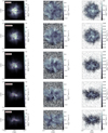 |
Fig. A.1 Same as Fig. 3 but for the HCO+ (J = 1 → 0) transition. |
| In the text | |
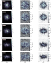 |
Fig. A.2 Same as Fig. 3 but for the HCN (J = 1 → 0) transition. |
| In the text | |
|
Fig. A.3 Same as Fig. 3 but for the N2H+ (J = 1 → 0) transition. In contrast to the other species studied here, N2H+ is a good tracer of the column density for most projection angles. |
| In the text | |
Current usage metrics show cumulative count of Article Views (full-text article views including HTML views, PDF and ePub downloads, according to the available data) and Abstracts Views on Vision4Press platform.
Data correspond to usage on the plateform after 2015. The current usage metrics is available 48-96 hours after online publication and is updated daily on week days.
Initial download of the metrics may take a while.