Which molecule traces what: Chemical diagnostics of protostellar sources

Łukasz Tychoniec; Ewine F. van Dishoeck; Merel L. R. van ’t Hoff; Martijn L. van Gelder; Benoît Tabone; Yuan Chen; Daniel Harsono; Charles L. H. Hull; Michiel R. Hogerheijde; Nadia M. Murillo; John J. Tobin

doi:10.1051/0004-6361/202140692

Home

All issues

Volume 655 (November 2021)

A&A, 655 (2021) A65

Full HTML

Free Access

Issue		A&A Volume 655, November 2021


Article Number		A65
Number of page(s)		38
Section		Interstellar and circumstellar matter
DOI		https://doi.org/10.1051/0004-6361/202140692
Published online		18 November 2021

A&A 655, A65 (2021)

Which molecule traces what: Chemical diagnostics of protostellar sources

Łukasz Tychoniec¹^,2, Ewine F. van Dishoeck²^,3, Merel L. R. van ’t Hoff⁴, Martijn L. van Gelder², Benoît Tabone², Yuan Chen², Daniel Harsono⁵, Charles L. H. Hull⁶^,7, Michiel R. Hogerheijde²^,8, Nadia M. Murillo⁹ and John J. Tobin¹⁰

¹ European Southern Observatory, Karl-Schwarzschild-Strasse 2, 85748 Garching bei München, Germany
e-mail: lukasz.tychoniec@eso.org
² Leiden Observatory, Leiden University, PO Box 9513, 2300 RA Leiden, The Netherlands
³ Max-Planck-Institut für Extraterrestrische Physik, Giessenbachstrasse 1, 85748 Garching, Germany
⁴ Department of Astronomy, University of Michigan, 500 Church Street, Ann Arbor, MI 48109, USA
⁵ Institute of Astronomy and Astrophysics, Academia Sinica, No. 1, Sec. 4, Roosevelt Road, Taipei 10617, Taiwan
⁶ National Astronomical Observatory of Japan, NAOJ Chile, Alonso de Córdova 3788, Office 61B, 7630422, Vitacura, Santiago, Chile
⁷ Joint ALMA Observatory, Alonso de Córdova 3107, Vitacura, Santiago, Chile
⁸ Anton Pannekoek Institute for Astronomy, University of Amsterdam, Science Park 904, 1098 XH Amsterdam, The Netherlands
⁹ Star and Planet Formation Laboratory, RIKEN Cluster for Pioneering Research, Wako, Saitama 351-0198, Japan
¹⁰ National Radio Astronomy Observatory, 520 Edgemont Road, Charlottesville, VA 22903, USA

Received: 1 March 2021
Accepted: 8 July 2021

Abstract

Context. The physical and chemical conditions in Class 0/I protostars are fundamental in unlocking the protostellar accretion process and its impact on planet formation.

Aims. The aim is to determine which physical components are traced by different molecules at subarcsecond scales (<100–400 au).

Methods. We used a suite of Atacama Large Millimeter/submillimeter Array (ALMA) datasets in band 6 (1 mm), band 5 (1.8 mm), and band 3 (3 mm) at spatial resolutions 0.″5–3″ for 16 protostellar sources. For a subset of sources, Atacama Compact Array (ACA) data at band 6 with a spatial resolution of 6″ were added. The availability of low- and high-excitation lines and data on small and larger scales, is important to understand the full picture.

Results. The protostellar envelope is well traced by C¹⁸O, DCO⁺, and N₂D⁺, which stems from the freeze-out of CO governing the chemistry at envelope scales. Molecular outflows are seen in classical shock tracers such as SiO and SO, but ice-mantle products such as CH₃OH and HNCO that are released with the shock are also observed. The molecular jet is a key component of the system. It is only present at the very early stages, and it is prominent not only in SiO and SO, but occasionally also in H₂CO. The cavity walls show tracers of UV-irradiation such as C₂H, c-C₃H₂ and CN. In addition to showing emission from complex organic molecules (COMs), the hot inner envelope also presents compact emission from small molecules such as H₂S, SO, OCS, and H¹³CN, which most likely are related to ice sublimation and high-temperature chemistry.

Conclusions. Subarcsecond millimeter-wave observations allow us to identify these (simple) molecules that best trace each of the physical components of a protostellar system. COMs are found both in the hot inner envelope (high-excitation lines) and in the outflows (lower-excitation lines) with comparable abundances. COMs can coexist with hydrocarbons in the same protostellar sources, but they trace different components. In the near future, mid-infrared observations with JWST–MIRI will provide complementary information about the hottest gas and the ice-mantle content, at unprecedented sensitivity and at resolutions comparable to ALMA for the same sources.

Key words: stars: formation / astrochemistry / techniques: interferometric / ISM: molecules / submillimeter: ISM

© ESO 2021

1 Introduction

The formation of Sun-like stars is set in motion by the collapse of a cold, dense cloud. Many different physical processes take place in the protostellar stage, which encompasses the first few 10⁵ yr that are critical to the subsequent evolution of the star and its planetary system (Lada 1987). The mass of the star and that of its circumstellar disk are determined during this embedded phase (Hueso & Guillot 2005), and the first steps of planet formation must take place then (Greaves & Rice 2010; Williams 2012; ALMA Partnership 2015; Manara et al. 2018; Harsono et al. 2018; Tobin et al. 2020; Tychoniec et al. 2018, 2020; Segura-Cox et al. 2020). On larger scales, the collapsing envelope is simultaneously dispersed by the energetic action of bipolar jets and winds emanating from the star-disk system, which creates outflows of entrained gas and dust (Arce & Sargent 2006; Offner & Arce 2014)

Rotational transitions of molecules are a powerful tool to probe other components of the system and can be used to infer densities, temperatures, UV fields, chemical abundances, and kinematics (van Dishoeck & Blake 1998; Evans 1999). Until recently, studies of low-mass protostars were hampered by spatial resolution that was insufficient to distinguish these different physical components. The advent of submillimeter interferometry opened the possibility of studying protostellar systems at much smaller scales than with single-dish observations (e.g., Chandler & Carlstrom 1996; Hogerheijde et al. 1999; Schilke et al. 1992; Wilner et al. 2000; Jørgensen et al. 2005a; Tobin et al. 2011).

With the Atacama Large Millimeter/submillimeter Array (ALMA), it is possible to image many molecular lines on the relevant physical scales with achievable observing times at subarcsecond resolution. Impressive ALMA studies of individual low-mass protostars have been presented, focusing both on simple species (<6 atoms) and complex molecules (>6 atoms) (e.g., Sakai et al. 2014a; Jørgensen et al. 2016; López-Sepulcre et al. 2017; Lee et al. 2019a,b; Codella et al. 2018; Manigand et al. 2020; van Gelder et al. 2020; Bianchi et al. 2020). The first ALMA surveys of complex molecules on a larger sample (Yang et al. 2021) and of Class I disks are currently conducted (Podio et al. 2020; Garufi et al. 2021). The Continuum and Lines in Young ProtoStellar Objects (CALYPSO) survey with IRAM Plateau de Bure Interferometer (PdBI) studied a larger sample of protostars, but at more limited resolution and sensitivity (Belloche et al. 2020; Maret et al. 2020; Podio et al. 2021).

We present ALMA data of 16 protostellar sources covering rotational transitions of various molecules. We used these data to build a complete picture of the physical structures in protostars that are traced by these types of molecules. This sample constitutes one of the largest combinations of high-resolution ALMA observations of Class 0/I protostars to date in ALMA bands 3, 5, and 6. The data cover a broad range of protostellar properties within the low-mass regime, and our aim is to identify and describe key molecular tracers of future Sun-like stars and the physical components of star-forming sources to which they correspond. Parts of the ALMA datasets presented here have been published before with focuses on different aspects: complex organic molecules (van Gelder et al. 2020; Nazari et al. 2021), the temperature structure of Class I disks (van ’t Hoff et al. 2020a), outflows and high-velocity jets in Serpens (Hull et al. 2016; Tychoniec et al. 2019), and molecular emission associated with magnetic fields (Hull et al. 2017; Le Gouellec et al. 2019). We provide a comprehensive overview of these different datasets and make full use of the observations with uniform analysis methods. This allows to reveal and systematise the molecular tracers of Class 0/I protostars. Out of 16 presented sources, 11 are included in upcoming James Webb Space Telescope (JWST) observations with the Mid-Infrared Instrument (MIRI; Wright et al. 2015) (Van Dishoeck et al. 2017; Ray et al. 2017) and the Near-Infrared Spectrograph (NIRSpec) (Van Dishoeck et al. 2017; Greene et al. 2017; Tobin et al. 2021; Harsono et al. 2021)

Class 0 sources are defined by the strong excess of their submillimeter luminosity and very low bolometric temperatures <70 K (André et al. 1993; Chen et al. 1995). These sources are associated with powerful outflows, and the envelope mass dominates the mass of the entire system. Class I sources are defined by having an infrared spectral index that indicates strong reddening (Lada 1987), with bolometric temperatures of 70–650 K (Chen et al. 1995). These systems have already converted most of their envelope mass into the disk and protostar (Crapsi et al. 2008; van Kempen et al. 2009b; Maury et al. 2011). For the typical envelope masses of the sources presented here and for the average disk masses found by Tychoniec et al. (2020), the masses are M_disk∕M_env ≃ 1% for Class 0 and ≃20% for Class I, with values up to 75–98% in cases of rotationally supported disks (Jørgensen et al. 2009).

The different components of protostellar systems vary significantly in their physical conditions, such as density and temperature, molecular enrichment, and dynamics. Our current knowledge about them is described briefly below to set the scene for the interpretation of our data.

Envelope

The envelope surrounding a protostar is the material that fuels the accretion process onto the star and disk. The physical conditions in the outer envelope on scales of a few 1000 au are reminiscent of those of starless cores with heavy freeze-out, and their chemical composition is directly inherited from the cloud out of which the star is being born (Caselli & Ceccarelli 2012). Systematic motions such as infall or expansion can occur, but otherwise, they are characterized by low turbulence and narrow (FWHM < 0.5–1 km s⁻¹) line profiles indicative of quiescent gas (Jørgensen et al. 2002).

Warm inner envelope

In the innermost part of the envelope on scales of the disk, the temperatures rise above 100 K so that any water and complex organic molecules (COMs) contained in ices are released from the grains back into the gas, where they are readily observed at submillimeter wavelengths. This region with its unique chemical richness is called the hot core, or to distinguish it from its high-mass counterpart, the hot corino (Herbst & van Dishoeck 2009).

Jets and outflows

As the material is accreting from the envelope onto the disk, excess angular momentum has to be transported in a still unexplained process to allow material to accrete onto the growing protostar. Jets and outflows constitute compelling candidates for extracting angular momentum through magnetic fields. In the earliest stages when the mass loss is highest, the densities are high enough to form molecules in the internal shocks in the jet (Bachiller & Gomez-Gonzalez 1992; Tafalla et al. 2010). Much slower (<20 km s⁻¹) and less collimated gas moving away from the protostar is called an outflow. The origin of the outflows remain debated. Large-scale outflows reveal bow-shock shells and cavities that may be driven by the fast intermittent jet (Gueth et al. 1996; Gueth & Guilloteau 1999; Tychoniec et al. 2019). The temperatures in shocked regions are much higher than in the surrounding envelope, up to a few thousand Kelvin, and sputtering of grain cores and ice mantles can further result in unique chemical signatures (Arce et al. 2008; Flower & Pineau des Forêts 2013).

Outflow cavity walls

These are the narrow zones in between the cold dense quiescent envelope material and the lower-density warm cone where outflows are propagating at high velocities. Cavity walls are exposed to UV radiation from the accreting star-disk boundary layer, which can escape through the outflow cavity without being extincted (Spaans et al. 1995). This creates conditions similar to those found in photon-dominated regions (PDRs), which occur throughout the interstellar medium near sources of intense UV radiation (Hollenbach & Tielens 1997). In units of the interstellar radiation field (ISRF, Draine 1978), typical values of 10² –10³ are found on scales of ~1000 au (van Kempen et al. 2009a; Y"i"ld"i"z et al. 2012; Benz et al. 2016; Karska et al. 2018).

Young disk

In the inner envelope, a protoplanetary disk starts to form as the natural outcome of a rotating collapsing core (Ulrich 1976; Cassen & Moosman 1981; Terebey et al. 1984). A young disk should be rotating in Keplerian motion. At early stages, it is difficult to identify whether the so-called embedded disk is rotationally supported because any molecular emission from the disk is entangled with that from the envelope. In recent years, several embedded disks have been identified to have Keplerian rotational structure on scales of ~100 au (Tobin et al. 2012; Murillo et al. 2013; Ohashi et al. 2014; Yen et al. 2017). Molecular tracers in young disks can probe their temperature structure in addition to providing kinematic information (van ’t Hoff et al. 2018b).

This work is organized as follows. In Sect. 2 we describe the observations we used, and Sect. 3 presents the results of this work, including detections and morphology of the targeted molecules. In Sect. 4 the results are discussed, with special focus on which molecular tracers correspond to each of the physical components. The focus ison a qualitative description, rather than quantitative analyses, for which source specific models and more rotational transitions of a given molecule are required. We summarize our work in Sect. 5.

Table 1

Targeted protostellar systems.

2 Observations

2.1 Datasets

Six different ALMA 12 m datasets at band 3, 5, and 6 are used in this work to cover 14 out of 16 sources. The spatial resolution of all ALMA 12 m datasets is comparable (0.″3–0.″6), except for 2017.1.01174.S, where band 3 observations are obtained at 3′′. Additionally, ACA observations with 7 m antennas were obtained for 5 out of 16 sources observed with band 6 at 6′′ resolution.

The targeted protostars are well-known objects located in different star-forming regions. They span a range of properties within the low-mass regime; the probed range of L_bol, T_bol, and M_env is shown in Table 1. The parameters are provided by a suite of observations across the infrared and submillimeter spectrum (Enoch et al. 2009; Kristensen et al. 2012; Green et al. 2013).

The details of the observations are summarized in Table A.1. The spatial resolution allows observing protostellar systems at solar system scales. Band 5 and 6 observations provide a resolution of ~0.′′5, which corresponds to a 70–220 au diameter for sources in our sample. Thus, regions down to 35–110 au radius in the inner envelope are probed. The band 3 data achieve a moderate resolution of ~3′′, which provides information on intermediate envelope scales of 500–1500 au. The ACA observations of six sources at 6′′ resolution probe envelope scales of 800–2000 au.

2.2 Spectral setup of the observations

A collection of different datasets using different ALMA bands implies varying spectral and spatial resolution and varying spectral coverage in the analysis. Throughout this paper, the sources shown in the figures therefore differ when detections and maps of different molecules are presented. In all cases, we discuss only those sources for which the given transition has been targeted when the molecule is discussed. All nondetections are explicitly stated. Table A.2 provides a list of targeted molecular transitions, including sources in which a particular line was covered and detected or not detected.

The ALMA observations presented here target different spectral setups across bands 3, 5, and 6. This allows probing the strongly varying physical scales and conditions. In particular, our band 3 data grant access to lines at very low excitation levels that enable tracing more extended material. Dust is less optically thick in band 3 than in band 6, which potentially allows insight into the densest inner regions. Band 6 offers a usual set of tracers of outflows: CO, SiO, and SO.

Cold outer envelopes with temperatures <20 K are probed with low E_up transitions. Additionally, nonthermal processes such as sputtering of material from the grains in the outflow are also observed in low E_up because their critical densities are low. On the other hand, thermal desorption from grains in the innermost regions are best probed with lines with high E_up. With the large span of frequencies of the observations, different transitions of the same molecule can be detected and used to trace different components of the system (e.g., an HNCO line at E_up = 15 K is available in band 3, and lines at 70 and 125 K are covered in band 6).

3 Results

3.1 Continuum emission from protostars

Figure 1 presents continuum emission maps toward four example protostars obtained with ALMA at ~0.′′5. The examples illustrate most of the characteristic features observed in the continuum maps. The continuum images for all sources are presented in Fig. B.1.

The continuum emission observed at millimeter wavelengths (1.3–3 mm in our observations) traces thermal dust emission from the inner envelope and the embedded disk. In the Class 0 protostars, the central continuum source generally appears compact R < 100 au (e.g., B1-c, Fig. 1). The example of SMM3 (Fig. B.1) shows a large resolved dust structure perpendicular to the outflow, but its classification as a disk is not certain. The fact that we observe primarily compact continuum emission toward Class 0 sources is consistent with observations of confirmed rotationally supported disks (e.g., Tobin et al. 2018, 2020; Maury et al. 2019) and predictions of models (Visser & Dullemond 2010; Harsono et al. 2015b; Machida et al. 2016). While we assume that this compact emission belongs to the young embedded disk, we do not have spatial and kinematic resolution to confirm the presence of Class 0 Keplerian disks in our sample.

The extended continuum emission in Class 0 sources is consistent with a significant amount of envelope material surrounding the protostar. In the case of the SMM1 system, presented in Fig. 1 (left), the continuum clumps outside the central emission are components of multiple protostellar systems, shown as stars, which is confirmed by individual molecular outflows (Hull et al. 2016, 2017). Binary components are also seen in TMC1, BHR71, and IRAS 4B (Fig. B.1). In the case of S68N presented in Fig. 1, two emission peaks that stand out from the diffuse envelope emission are indicated with circles, but their protostellar nature is not confirmed.

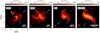Fig. 1

Continuum emission at 1.3 mm of four example protostellar systems obtained with ALMA at 0.′′5 resolution. Stars indicate confirmed protostellar sources, circles show condensations of continuum emission without confirmed protostellar nature, dotted lines show outflow cavity walls, and dashed lines show streams of envelope material. Arrows indicate outflow directions.

3.2 Protostellar envelope

We present molecules that trace the bulk of the protostellar envelope in Fig. 2. The protostellar envelope has a typical radius on the orderof a few 1000 au (Jørgensen et al. 2002; Kristensen et al. 2012). Thus, the subarcsecond ALMA 12 m array observations tend to resolve the envelope emission out. For instance, the maximum recoverable scale (MRS) of ALMA band 6 observations at 0.′′4 presented here is 5′′, which is between 600–2000 au diameter depending on the distance to the source. For this reason, we discuss in this section mainly the ALMA-ACA observations obtained at lower spatial resolution (6′′; 750–2500 au) for five sources in our datasets that are Class 0 sources: B1-c, BHR71, Per-emb-25, SMM3, and IRAS 4B, and for the Class I source TMC1. The ACA can zoom-in on what was previously contained in a single-dish beam of 15–20′′, while the MRS of ACA (30′′) enables us to preserve sensitivity to large-scale emission. The MRS of all observations presented here are reported in Table A.1.

In Fig.2 the typical envelope tracers C¹⁸O 2–1 (E_up = 16 K), DCO⁺ 3–2 (E_up = 21 K), and N₂D⁺ 3–2 (E_up = 22 K), observed at 6′′ resolution with the ACA, are presented toward the example Class 0 and Class I sources B1-c and TMC1, respectively. The emission from the presented molecules exhibits a similar behavior for all Class 0 sources, therefore B1-c serves as a representative case. TMC1 is the only Class I source in the sample for which 7 m observations are available. The maps for all sources in which these molecules were targeted are providedin Appendix C. All envelope tracers presented here are characterized by narrow line profiles with an FWHM ~ 1 km s⁻¹.

The C¹⁸O emission peak coincides with the continuum peak for our six sources and appears to be compact. The diameter is less than 1000 au for B1-c and TMC1. For B1-c and all Class 0 sources (Fig. C.1), low-level extended C¹⁸O emission is seen along the outflow direction. For the only Class I source targeted with the ACA, emission is marginally resolved in the direction perpendicular to the outflow.

In our observations, N₂D⁺ is seen extended in the direction perpendicular to the core major axis toward B1-c (Fig. 2) and other Class 0 sources except IRAS 4B (Fig. C.2). In the case of IRAS 4B, the emission from this molecule appears dominated by large-scale emission from the filament detected toward this source, which connects it with IRAS 4A (Sakai et al. 2012). The peak of the N₂D⁺ emission is significantly shifted from the continuum peak in all cases, with a significant decrease in the innerregions in some cases (see BHR 71 in Fig. C.2). Similar extended N₂D⁺ emission in other Class 0 sources was reported by Tobin et al. (2013) based on lower-resolution SMA and IRAM-30 m data. For TMC1, the N₂D⁺ molecule is not detected.

The DCO⁺ emission is seen extended in a similar way as for N₂D⁺. However, in contrast to N₂D⁺, DCO⁺ is brightest at the continuum peak for all sources except for TMC1 and Per-emb-25. For these two sources, the emission peak is offset by 1000–2000 au from the continuum source in the direction perpendicular to the outflow. In the Class I source TMC1, DCO⁺ is present on much smaller scales (<2000 au radius) than in Class 0 sources.

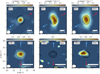Fig. 2

Maps of key envelope tracers toward B1-c (Class 0, top) and TMC1 (Class I, bottom) obtained with ACA. Contours represent continuum emission at 1.3 mm observed with ACA. Different distances to B1-c and TMC1 result in different spatial resolutions of the maps. Left: C¹⁸O 2–1. Middle: N₂D⁺ 3–2. Right: DCO⁺ 3–2. All moment-0 maps are integrated from −2.5 to 2.5 km s⁻¹ with respect to v_sys.

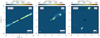Fig. 3

Maps of the EHV jets observed in SiO. Moment-0 maps are presented in color scale, in which continuum emission at 1.3 mm ispresented as black contours, both obtained with 12 m observations. SiO 4–3 map of HH211 integrated from −20 to −10 and from 10 to 20 km s⁻¹ with respect to v_sys, B1-c integrated from −70 to −40 and from 40 to 70 km s⁻¹ with respect to v_sys, and SMM3 integrated from −60 to −40 and from 20 to 35 km s⁻¹ with respect to v_sys.

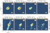Fig. 4

Zoom-in on molecular bullets from the SMM3 jet (see Fig. 3). CO, SiO, SO, and H₂ CO molecular transitions are presented. Top: northern blueshifted bullet. Moment-0 maps are integrated from –60 to –40 km s⁻¹ with respect to v_sys. The map center is offset from the SMM3 continuum center by (–3.′′7, +10.′′3). Bottom: southern redshifted bullet. Moment-0 maps are integrated from 20 to 40 km s⁻¹. The map center is offset from the SMM3 continuum center by (+2.′′7, –7.′′).

3.3 Outflows and jets

Figure 3 presents the extremely high-velocity (EHV) molecular jet component for HH211, B1c, and SMM3 observed in SiO with the ALMA 12 m array; the L1448-mm EHV is shown in figure later on. The latter and HH211 are well-known EHV sources (Guilloteau et al. 1992; Lee et al. 2007), while SMM3 and B1-c are new detections of the jet component. HH211 shows SiO emission at low velocities because the outflow is almost in the plane of the sky, but the high velocities are evident from the large proper motion movements of the bullets (~115 km s⁻¹; Lee et al. 2015). CO, H₂CO, and SiO in the EHV jets of Emb8N and SMM1 are presented in detail in Hull et al. (2016) and Tychoniec et al. (2019).

These data are particularly interesting because still only a few molecules that trace EHV jets have been identified to date (see Lee 2020 for review). In addition to those presented here, CO, SiO, SO, and H₂CO, molecules such as HCO⁺ and H₂O have been observed in this high-velocity component (Kristensen et al. 2012; Lee et al. 2014). It is especially important to highlight the third detection of a H₂CO bullet in SMM3 after IRAS 04166 (Tafalla et al. 2010) and Emb8N (Tychoniec et al. 2019). These detections mean that either a significant fraction of ice-coated dust is released with the jet, or that the H₂CO is efficiently produced in the jet through gas-phase chemistry.

Several molecular bullets are observed along the jet axis with velocities up to 100 km s⁻¹ in L1448-mm and HH211, while both B1-c and SMM3 show a much simpler structure in which two bullets are detected on one side in the former and a single pair of symmetrically placed bullets observed in the latter case. In B1-c a pair of bullets is located ~200 au from the continuum peak, and the other bullet at 2500 au is only seen in the redshifted part of the jet. The emission in SiO and SO appears to be very similar (Figs. D.2 and D.3). No other molecules trace the high-velocity component toward this source. H₂CO and ¹²CO are not targeted with our ALMA 12 m datasets toward B1-c. The SMM3 jet has two distinct high-velocity bullets at ~3200 au from thesource that appear to be similar in CO, SiO, and SO (see the zoom-in on Fig. 4). Additionally, the redshifted bullet shows faint but significant emission from H₂CO. No traces of H₂CO are found inthe blueshifted outflow.

Figure 5 presents low-velocity outflow tracers CO 2–1 (E_up = 16 K) for TMC1, SO 5₆ –4₅ (E_up = 35 K), and SiO 4–3 (E_up = 21 K) for B1-c. In Fig. D.1 we present an overview of the CO 2–1 emission for five sources obtained with the ALMA 12 m array at 0.′′4 resolution. The sources show a variety of emission structures in the low-velocity gas (<20 km s⁻¹). We do not capture the entirety of the outflows in none of the cases because they extend beyond the primary beam of observations (~30′′). SMM3 and Emb8N have very narrow outflow opening angles (<20 degrees), while SMM1, S68N, and TMC1 present larger opening angles.

CO emission is especially prominent in the cavity walls. This can be related to both the limb brightening effect and to the higher (column) density of the material in the outflow cavity walls. This is especially highlighted in the Class I source TMC1, where CO emission is almost exclusively seen in the outflow cavity walls. Even though CO is piling up in this region, it is observed at velocities up to 15 km s⁻¹, so that it clearly traces the entrained material and not the envelope. The lower envelope density in Class I results in less material that can be entrained in the outflow. Three CO outflows from SMM1-a, SMM1-b, and SMM1-d overlap in SMM1 (Hull et al. 2016; Tychoniec et al. 2019).

In Fig. D.2 we present SiO maps: band 5 SiO 4–3 (E_up = 21 K) and band 6 SiO 5–4 (E_up = 31 K) data are shown in velocity ranges corresponding to the low-velocity outflow. In contrast to CO emission, the low-velocity SiO is mostly observed in clumps of emission instead of tracing the entirety of the outflowing gas. Several such clumps are observed in source S68N. In some cases, the clumps are relatively symmetric (Emb8N and B1-c), while monopolar emission is seen in other examples (L1448-mm and SMM1-d). SMM1-a and SMM1-b show very weak SiO emission at low velocities. SiO emission in outflows is exclusively present in the Class 0 sources and is absent in the Class I sources TMC1 and B5-IRS1 that are covered in these data sets.

Figure D.3 presents SO 5₆ –4₅ (E_up = 35 K) and SO 6₇ –5₆ (E_up = 47 K) observations in band 6. The emitting regions of SO are comparable with those of SiO for the Class 0 sources. The cases of S68N and B1-c show that SO emission also peaks at the source position, but SiO is absent there. This shows that SO and SiO do not always follow each other, and some SO might be associated with hot-core emission (Drozdovskaya et al. 2018). Important differences are observed for TMC1, where SO seems to be associated with the remainder of the envelope or the disk, while SiO is not detected toward this source, as mentioned above.

HCN 1–0 (E_up = 4 K) and H¹³CN 2–1 (E_up = 12 K) maps arepresented in Figs. D.4 and D.5, respectively. HCN is clearly seen in outflowing material enhanced in similar regions as the low-velocity SiO. For Emb8N, the HCN emission has been associated with an intermediate-velocity shock (Tychoniec et al. 2019). In B1-c and L1448-mm, weak extended emission along the outflow direction is detected, but H¹³CN strongly peaks at the source. HH211 shows H¹³CN only in the outflow, and the geometry is consistent with the outflow cavity walls, but the velocity profiles are consistent with the outflowing material.

Ice-mantle tracers are a different class of molecules that are detected in low-velocity protostellar outflows. They are produced and entrained through interactions between the jet and the envelope. Here we present ALMA 12 m array observations in band 6 at 0.′′5 resolution for CO 2–1 (E_up = 17 K), CH₃OH 2_1,0 –1_0,0 (E_up = 28 K), and H₂CO 3_0,3 –2_0,2 (E_up = 21 K), and in band 3 at 3′′ resolution for CH₃CN 6₁ –5₁ (E_up = 26 K), CH₃CHO 6_1,6,0 – 5_1,5,0 (E_up = 21 K), and HNCO 5_0,5 –5_0,4 (E_up = 16 K). Figure 6 compares maps of integrated emission from these molecules with those of CO for S68N. All ice-mantle tracers detected in the outflow are observed in their low-energy transitions. Additional maps for S68N are presented in the appendix (Fig. D.6): band 6 0.′′5 resolution image of CH₃CHO 14_0,14–13_0,13 (E_up = 96 K) and H₂ CCO 13_1,13–12_1,12 (E_up = 101 K), which overlaps with NH₂CHO 12_2,10–12_2,10 (E_up = 92 K), and the band 3 image at 3′′ resolution of CH₃OCHO 10_0,10–9_0,9 (E_up = 30 K).

Around the frequency of the H₂ CCO 3_1,13–12_1,12 (E_up = 101 K) line, an extended emission is observed in the outflow, but it is coincident with NH₂CHO, which is only 4 km s⁻¹ apart (Fig. D.6). NH₂CHO is more commonly observed in the shocked regions than H₂CCO (Ceccarelli et al. 2017; Codella et al. 2017); it is possible that these lines are blended. More low-energy transitions are required to confirm the identification of these lines.

The velocities observed for ice-mantle tracers in the outflow are <15 km s⁻¹ with respect to the systemic velocity. This is slower than the CO and SiO outflow line wings, which have velocities up to 20–30 km s⁻¹. On the other hand, the lines are clearly broader than those of molecular tracers of UV-irradiated regions that trace passively heated gas (see Sect. 4.3).

Ice-mantle tracers are also detected in SMM3 and B1-c, two Class 0 protostars (Figs. D.7 and D.8). For SMM3, only a lower A_ij transition of CH₃OH with E_up = 61 K was targeted, but not detected toward this source. The methanol emission of B1-c is confused with the high-velocity SO emission, whereas emission from other COMs in the outflow is weak and only appears in the redshifted part of the outflow. Thus, S68N is the best case to study the composition of shock-released ice mantles.

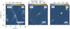Fig. 5

Low-velocity outflow in CO, SO, and SiO. The moment-0 maps of CO toward TMC1 and the SO and SiO map toward B1c are integrated from −10 to 10 km s⁻¹ with respect to v_sys.

3.4 Outflow cavity walls

In this section, we highlight key molecules detected in the outflow cavity walls. It is challenging to precisely distinguish cavity walls from the outflowing material. The velocity of the gas in the cavity walls should be lower than in the outflow because the cavity wall contains envelope material at rest that is passively heated by UV radiation, however. We first discuss maps of species associated with cavity walls and then their line profiles.

Figure 7 presents integrated emission maps of key tracers discussed in this section for two examples: SMM3 and B1-c. Plots for the remaining sources (S68N, Emb8N, and TMC1) are presented in the appendix in Fig. E.1. Key tracers of the outflow cavity walls are simple unsaturated hydrocarbon molecules: c-C₃H₂ 4_4,1 –3_3,0 (E_up = 32 K) for SMM3 and TMC1, and C₂H 3_2.5,3–2_1.5,2 (E_up = 25 K) for S68N, B1-c, and Emb8N, as seen in maps obtained with ALMA band 6 at 0.′′5 resolution.

In Emb8N and SMM3 the emission from C₂H and c-C₃H₂, respectively,is symmetric. It appears similar in extent and shape on either side of the continuum source. Comparison with CO emission, which traces the bulk of the outflowing gas, indicates that the hydrocarbons are located in the outflow cavity walls close to the source. A higher-energy transition of c-C₃H₂ 7_2,6 –7_1,7 E_up = 61 K is seen toward SMM3 closer to the protostar than the lower-energy transition. This reflects the increase in temperature of the cavity walls closer to the source. For B1-c, the emission from C₂H is U-shaped, suggestive of a cavity wall, and it is stronger on the blueshifted side of the outflow, which could be either a projection effect or an asymmetry in the envelope structure. For B1-c, no ALMA CO observations exist to compare with the bulk of the outflow at comparable resolution, but the other outflow tracer SO confirms the outflow direction and approximate extent of the outflow cavity walls. Moreover, the shape of the cavity walls is consistent with the appearance of the CO 3–2 outflow observed with SMA toward this source at 4′′ resolution (Stephens et al. 2018).

S68N presents a chaotic structure (Fig. E.1, top), but C₂H is found to be elongated in the outflow direction. While it is difficult to identify the cavity wall, the C₂H emission surrounds the CO outflow emission. The C₂H emission toward this source is asymmetric, with stronger emission in the blueshifted part of the outflow. Emission of c-C₃H₂ toward the Class I source TMC1 (Fig. E.1, bottom) is not directly related to the cavity walls, but is extended perpendicular to the outflow, which suggests that c-C₃H₂ traces the envelope or extended disk material.

Figure 7 also shows CN 1–0 (E_up = 5 K) observed at 3′′ resolution in band 3 for SMM3 and B1-c. Compared with C₂H, CN traces similar regions. In S68N, CN has a similar extent as C₂H, but not over the full extent of the outflow traced by CO. In B1-c, the CN emission has a similar shape of the cavity wall cone as observed in C₂H, but a significant contribution from larger scales is also detected. In all cases, the CN emission avoids the central region, which likely results from on-source absorption by the foreground CN molecules.

In some cases such as SMM3, the extent of the CN is broader than the extent of hydrocarbons, which are more comparable with CO. The narrow line widths suggest, however, that this emission is still associated with the passively irradiated envelope rather than with the entrained outflow.

TMC1 presents a high-resolution example of CN emission (Fig. E.1). The offset between CO and CN reveals the physical structure of the inner regions of the protostellar system: the entrained outflow traced with CO appears to be closer to the jet axis, while CN highlights the border between the outflow cavity wall and the quiescent envelope. CN is sensitive to UV radiation because it can be produced with atomic C and N, whose abundances are enhanced in PDRs, and UV photodissociation of HCN contributes as well (Fuente et al. 1993; Jansen et al. 1995; Walsh et al. 2010; Visser et al. 2018).

H¹³CO⁺ emission is presented for B1c (Fig. 7), S68N, and Emb8N (Fig. E.1) observed in band 6 at 0.′′4 resolution. The bulk of the emission from this molecule appears to be related to the cold envelope, but streams of material are observed in B1-c and S68N. Examples of such streamers kinematically consistent with accretion have been observed in other protostars (Pineda et al. 2020). The streams of gas observed in H¹³CO⁺ are coincident with the cavity wall observed in C₂H. Because H¹³CO⁺ is expected to probe the dense envelope, the similarity of the morphology of the traced material between H¹³CO⁺ and C₂H and CN shows that the envelope material is UV irradiated. ¹³CS observed in band 6 with the 12 m array is detected for SMM3 (Fig. 7). The morphology of ¹³CS emission is very similar to that of c-C₃H₂.

In Fig. 8 we present spectra of the ice-mantle tracers CH₃OH and H₂CO and the hydrocarbon molecules C₂H and C₃H₂. All spectra are shifted by their source velocity to zero km s⁻¹. In case of S68N, C₂H and CH₃OH have very similar line profiles, indicating that they trace similar material. The width of ~ 10 km s⁻¹ suggests that this material is entrained with the outflow. A narrow component appears to be superposed at systemic velocities. Fine-splitting of C₂H blends the spectra, although the other transition at +2 km s⁻¹ does not affect the blueshifted velocity component. In contrast, B1c shows only remarkably narrow C₂H line profiles with an FWHM of ~2 km s⁻¹, and SMM3 has similarly narrow c-C₃H₂ and ¹³CS lines compared with the broader H₂CO emission (Fig. 8, right).

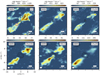Fig. 6

Maps of the ice mantle tracers toward the S68N outflow, with the CO low-velocity outflow map for reference. Top: CO, H₂CO, and CH₃OH moment-0 maps obtained in band 6 at 0.′′5 resolution. Circles show regions from which spectra were obtained for the analysis in Sect. 7.1. Bottom: CH₃CHO, HNCO, and CH₃CN moment-0 maps obtained in band 3 at 2.′′5 resolution. The emission is integrated from −10 to −1 km s⁻¹ and from 1 to 10 km s⁻¹ with respect to v_sys.

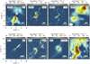Fig. 7

Maps of the outflow cavity wall tracers toward SMM3 and B1c, with the low-velocity outflow map for reference. Top: moment-0 maps toward SMM3 of CO 2–1, c-C₃H₂ 6_1,6 –5_0,5, and ¹³CS 5–4 obtainedin band 6 at 0.′′5 resolution and CN 1–0 in band 3 at 3′′ with continuum emission at the same band and the resolution shown as black contours. Bottom: moment-0 maps toward B1c of SO 6₇–5₆, C₂H 3_2.5,3 –2_1.5,1, and H¹³CO⁺ 3–2 obtainedat 0.′′5 and CN 1–0 at 3′′ resolution with continuum emission at the same band and the resolution shown as black contours. The emission is integrated from −5 to −1 km s⁻¹ and from 1 to 5 km s⁻¹ with respect to v_lsr. Outflow directions and delineated cavity walls are shown in C₂H and C₃H₂ maps.

3.5 Inner envelope

Figure 9 shows emission from H₂CCO, HNCO, t-HCOOH, SO, H₂CS, and H¹³CN for the Class 0 protostar B1-c and H₂S and OCS lines for SMM3; all observed with the ALMA 12 m array at 0.′′5. Several molecules tracing the inner hot envelope are detected in 7 m data and are presented in Fig. F.1. CCS is detected for SMM3, BHR71, and IRAS 4B, but it is nondetected for B1-c, TMC1, and Per-emb-25. OCS and H₂S (Fig. F.1) are observed for all targeted in 7 m Class 0 sources, but are nondetected for Class I sources.

The SO 6₇–5₆ E_up = 48 K line is observed to peak on the central source for B1-c and S68N (Fig. D.3). SO has already been discussed in the outflow (Sect. 4.2.2), but it is also prominent in the inner envelope. While the spatial resolution does not allow us to distinguish the hot-core emission from the small-scale outflow on a scale of a few hundred au, there is a difference between these two sources and SMM3 and Emb8N. The latter two sources show a substantial decrease in SO intensity toward the continuum peak, that is, they have prominent SO emission in the outflow, but not from the hot core. This suggests that in sources like B1-c and S68N, which are bright in SO toward the continuum emission peak, an additional component causes the SO emission. This is highlighted by the narrower lines of SO toward the continuum peak compared with the outflow in S68N (Fig. G.1). The narrow component, visible in spectra taken on-source, has a width of ~5 km s⁻¹. The main component of the spectrum taken in the blueshifted outflow has a similar width, but a more prominent line wing up to 20 km s⁻¹.

TMC1 clearly shows SO emission toward both components of the binary system, slightly offset from their peak positions (Fig. D.3). A molecular ridge is also present in SO close to the disk-envelope interface.

HNCO and HN¹³CO are detected toward B1-c and S68N peaking on-source in higher E_up transitions (Nazari et al. 2021). For lines with E_up < 90 K, an extended component is also detected in the outflow. SMM3 and Emb8N have no detections of HNCO on-source, but for SMM3, this molecule appears in the outflow. For none of the Class I sources in which the relatively strong HNCO 11_0,11–10_0,10 line (A_ij = 2 × 10⁻⁴ s⁻¹, E_up = 70 K) was targeted was it detected.

OCS is detected toward SMM3 peaking in the center; S68N and SMM1 show centrally peaked O¹³ CS detection. This is a minor isotopolog signalling a high abundance of OCS (Fig. F.2). In all cases, the emission is moderately resolved. It extends to ~200 au in the case of SMM3 and is detected up to 500 au away from source for S68N and SMM1.

H₂S shows strong emission toward SMM3 and is also weakly present in TMC1. For SMM3, the emission is resolved along the outflow direction and perpendicular to the expected disk axis. These are the only two sources for which H₂S 12 m array data were taken. Additionally, the 7 m data presented in the appendix (Fig. F.1) show prominent centrally peaked H₂S emission for four more Class 0 sources.

H₂CS is detected for B1-c, S68N, and L1448-mm through a line with E_up = 38 K. Another transition with E_up = 46 K is found in Class I disks: IRAS-04302, L1489, and TMC1A. In B1-c, the emission is marginally resolved, while in IRAS-04302 the molecule is clearly observed across the midplane, indicating sublimation from icy grains at temperatures of at least 20 K (van ’t Hoff et al. 2020a; Podio et al. 2020).

H₂CCO is detected for B1-c and S68N. For the lower E_up = 100 K transition, the molecule is also detected in the outflow. For Class I sources, the transition at comparable energy is not detected. HCOOH is detected for B1-c and S68N with low-energy transitions that are seen both on-source and in the outflow, while the higher-energy line (E_up = 83 K) is only observed on-source. H¹³CN is detected in B1-c and L1448-mm on-source in addition to the outflow component.

Disks are commonly observed in Class I sources (Harsono et al. 2014; Yen et al. 2017) as the envelope clears out material from the gap. Fig. 10 presents maps of the C¹⁷O 2–1 (E_up = 16 K) and CN 2–1 (E_up =16 K) lines toward Class I disks and L1527-IRS, which is identified as a Class 0/I object, observed with ALMA 12 m at 0.′′3 resolution. The C¹⁷O and H₂CO emission for disks in Taurus using these data were analyzed in detail by van ’t Hoff et al. (2020a). Here we discuss CN in comparison with C¹⁷O. C¹⁷O is observed to be concentrated toward the continuum emission for all disks, and is a much more unambiguous tracer of the disk than any other more abundant CO isotopolog, although even C¹⁷O still shows some trace emission from the surrounding envelope.

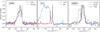Fig. 8

Spectra obtained at the cavity wall positions for hydrocarbons (red) and ice-mantle tracers (blue). Left: C₂H 3_2.5,2 –2_1.5,1 (E_up = 25 K) and CH₃OH 2_1,0 –1_0,1 (E_up = 28 K) spectra for S68N. Middle: C₂H 3_2.5,2 –2_1.5,1 (E_up = 25 K) and SO 6₇–5₆ (E_up = 48 K) spectra for B1-c. Right: c-C₃H₂ 4_4,1 –3_3,0 (E_up = 32 K), H₂CO 3_2,1 –2_2,0 (E_up = 68 K), and ¹³CS 5–4 (E_up = 33 K) spectra for SMM3.

4 Discussion

Figure 11 summarizes the current understanding of which components are traced by the molecules in Class 0/I protostars. Table 2 lists all molecules discussed in this work and indicates the physical component that they trace. Below, we address several implications of the results. We note that the discussion is confined to the molecules that were targeted and detected in our datasets, but it is by no means complete. Other relevant tracers not discussed here are NH₃ and N₂H⁺, which trace the envelope well (e.g., Tobin et al. 2011; Chen et al. 2007; Pineda et al. 2019). PO and PN were recently suggested as cavity wall or outflow tracers, but their abundances are very low (Bergner et al. 2019). SO₂ is an important tracer of thewarm gas in the disk-envelope interface (Artur de la Villarmois et al. 2019). Finally, we focused on low-energy transitions observed with ALMA E_up < 100 K, with the exception of hot core tracers.

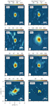Fig. 9

Compact emission for B1-c and SMM3 for various molecules tracing the warm inner envelope (hot core). Moment-0 maps shown in color scale integrated from −3 to 3 km s⁻¹ with respect to v_sys. The 1.3 mm continuum is presented as contours.

4.1 Cold envelope

4.1.1 C¹⁸O

C¹⁸O is a good tracer of high column density material because its critical density is low. However, it becomes less abundant as soon as the dust temperature drops below the CO freeze-out temperature (~20–25 K). There is also a density threshold: CO freeze-out only occurs at densities above ~ 10⁴–10⁵ cm⁻³ because at lower densities, the timescales for freeze-out are longer than the lifetime of the core (Caselli et al. 1999; Jørgensen et al. 2005b).

For four out of the six sources presented here at 6′′ resolution, Kristensen et al. (2012) modeled the SED and submillimeter spatial extent using the code DUSTY (Ivezic & Elitzur 1997). Among other properties, the results provide a temperature structure throughout the envelope and the radius at which the temperaturedrops below 10 K, which is considered as the border between envelope and the parent cloud. Kristensen et al. (2012) obtained radii of 3800, 5000, 6700, and 9900 au for IRAS 4B, TMC1, SMM3, and BHR71, respectively. The compact C¹⁸O emission observed on-source and its nondetection over the full expected extent of the protostellar envelope can be explained by CO freeze-out occurring already within the inner 1800–2500 au radius, which is the spatial resolution of our observationsfor Class 0 sources. This upper limit on the CO snow line is consistent with CO snow lines that are typically observed and modeled toward other Class 0 protostars (Jørgensen et al. 2004a; Anderl et al. 2016; Hsieh et al. 2019).

Equation (1) from Frimann et al. (2017) allows calculating the expected CO snow line for the current luminosity of the example sources B1-c and TMC1 presented in Fig. 2 in the absence of an outburst. For B1-c the snow line is expected to be at 200–400 au radius depending on the assumptions of the sublimation temperature (larger radii for 21 K and smaller for 28 K), while the TMC1 CO snow line is expected to be at 100–200 au. For the most luminous source with C¹⁸O 7 m observations available, the expected radius is at 400–750 au. This means that in all cases, the expected CO snow line is clearly well within the 7 m beam. In high-resolution studies, the CO emission is often seen at greater distances than expected from the current luminosities of these protostars. This is attributed to accretion bursts of material that increase their luminosities, resulting in a shift of the observed CO emission radius up to a few times its expected value (but usually still within a 1000 au radius) (Jørgensen et al. 2015; Frimann et al. 2017; Hsieh et al. 2019).

4.1.2 N₂D⁺ and DCO⁺

Both DCO⁺ and N₂D⁺ are considered cold gas tracers (e.g., Qi et al. 2015). N₂D⁺ is efficiently destroyed by CO in the gas phase, therefore freeze-out of CO results in N₂D⁺ being retained in the gas phase at larger radii of the envelope, where temperatures are lower. This behavior has been demonstrated in several other protostellar sources by Tobin et al. (2011, 2013, 2019).

Both DCO⁺ and N₂D⁺ are produced through reactions with H₂ D⁺. At cold temperatures, the H₂ D⁺ abundance is enhanced through the H $_{3}^{+}$ $_3^+$ + HD → H₂ D⁺ + H₂ reaction, which is exothermic by 230 K. As the reverse reaction is endothermic, low temperatures increase H₂ D⁺. Additionally, both H $_{3}^{+}$ $_3^+$ and H₂ D⁺ are enhanced in gas in which CO has been depleted. However, the CO molecule is still needed for the production of DCO⁺ through the H₂ D⁺ + CO reaction. Therefore DCO⁺ is expected to be most abundant around the CO snow line (Jørgensen et al. 2004a; Mathews et al. 2013). Warmer production routes through CH₂D⁺ + CO are also possible (Wootten 1987; Favre et al. 2015; Carney et al. 2018).

The difference between DCO⁺ and N₂D⁺ chemistry isreflected in the morphology of both molecules in the dense regions close to the continuum peak. As DCO⁺ requires gas-phase CO for its formation, it peaks close to the CO snow line, which is within the resolution of our observations (~1800–2500 au radius), while N₂D⁺ is only located where CO is not present in the gas phase. Therefore we observe a significant decrease in N₂D⁺ in the inner envelope. If the warm production of DCO⁺ is triggered in the inner regions, this will additionally produce DCO⁺ within the beam of our observations, hence DCO⁺ does not decrease in the inner envelope. The extent of the DCO⁺ and N₂D⁺ emission in each source is comparable, ranging from ~5000 au in B1-c and BHR71 to 1500 au in TMC1, suggesting that their outside radii trace the region in which CO becomes present again in the gas phase as a result of the low density.

The morphology of the emission from cold gas tracers such as DCO⁺ and N₂D⁺ is sensitive to the density and temperature profile of the system, which can be affected by the system geometry (i.e., outflow opening angle, disk flaring angle, and flattening of the envelope). DCO⁺ has been shown to increase its abundance in the cold shadows of a large embedded disk (Murillo et al. 2015). Emission from DCO⁺ and N₂D+ is consistent with a picture of a dissipating envelope in Class I sources, resulting in less dense, warmer gas surrounding the protostar. TMC1 has an order of magnitude lower envelope mass compared to the Class 0 sources (Table 1; Kristensen et al. 2012). This causes the extent of the cold and dense region to shrink, preventing N₂D⁺ from being detected, and limiting the extent of DCO⁺ emission. The dense gas toward TMC1 is clearly present only in the flattened structure surrounding the binary system, where it may form a young embedded disk. This source is suggested to have a rotationally supported circumbinary disk (Harsono et al. 2014; van ’t Hoff et al. 2020a). The geometry of the disk can create favorable conditions for the DCO⁺ enhancement in the cold shadows of the disk.

Other relevant molecules that trace the quiescent envelope material but are not presented here are HCO⁺ and H¹³CO⁺ (Hogerheijde et al. 1997; Jørgensen et al. 2007; Hsieh et al. 2019, van ’t Hoff et al. in prep.). These molecules have been shown to probe the material outside of the water snow-line (Jørgensen et al. 2013; van ’t Hoff et al. 2018a). As water sublimates at temperatures ~ 100 K, which is much higher than CO, HCO⁺ can be detected throughout the envelope, except for the warmest inner regions. N₂H⁺ traces the envelope material and CO snow line and has been shown to peak closer to the central protostar than N₂D⁺ (Tobin et al. 2013). Their ratio can potentially be used as an evolutionary tracer of protostars (Emprechtinger et al. 2009). NH₃ is also observed to map similar components as N₂H⁺ (Tobin et al. 2019).

In summary, the quiescent envelope material is traced by dense and/or cold gas tracers. Chemical interactions result in N₂D⁺ tracing the outer envelope where CO is frozen out, whereas DCO⁺ is detected both in the outer envelope and in the inner regions, where it traces the unresolved CO snowline. C¹⁸O is a good tracer of dense (n > 10⁵ cm⁻³) and warm (T > 30 K) regions in the inner 2000 au radius of the protostellar systems. The evolution of the physical conditions from Class 0 to Class I is evident as the envelope becomes less dense and the protostellar luminosity can more easily heat up dust and gas.

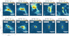Fig. 10

Images of Class I disks observed with ALMA 12 m in band 6 (van ’t Hoff et al. 2020a). Top: moment-0 maps of C¹⁷O at 0.′′4 resolution integrated from −10 to 10 km s⁻¹ with respect to v_sys. Bottom: moment-0 maps of CN integrated from −2 to 2 km s⁻¹ with respect to v_sys. Continuum contours are shown in black.

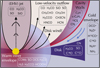Fig. 11

Summary cartoon presenting key molecular tracers of different components, limited to molecules presented in this work except for NH₃ and N₂H⁺, which are important large-scale envelope tracers. CN is shown on top of the disk as it traces the disk atmosphere and not the midplane. The protostar is indicated in yellow in the center.

Table 2

Molecular tracers of physical components exclusive to this work.

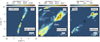Fig. 12

Maps of three different outflow components. Moment-0 maps are presented in color scale, and the continuum emission at 1.3 mm is plotted in black. Both were obtained with ALMA 12 m observations. Left: EHV molecular jet illustrated with the SiO (4–3) map for L1448-mm integrated from −70 to −50 and from 50 to 70 km s⁻¹ with respect to v_sys. Middle: low-velocity outflow illustrated with the CO 2–1 map for S68N integrated from −15 to −3 and from 3 to 15 km s⁻¹ with respect to v_sys. Right: ice-mantle content released with shock sputtering presented with the CH₃OH (2_1,0 – 1_0,0) map for S68N integrated from −8 to −1 and from 1 to 8 km s⁻¹ with respect to v_sys. The CO outflow from Ser-emb-8N is present at the edge of the map.

4.2 Outflows and jets

Outflowing material from protostellar systems is best analyzed with kinematic information. In the following section, we discuss three different components of protostellar outflows observed with the ALMA 12 m array: (1) the high-velocity jet (>30 km s⁻¹), (2) the low-velocity outflow (<30 km s⁻¹), and (3) the gas that results from the interaction with the outflow and ice-sputtering products at velocities close to that of the ambient material, but with significantly broader line widths (up to 15 km s⁻¹) than the quiescent envelope tracers. The three components are presented in Fig. 12 with examples of S68N, which is a representative case of a prominent outflow and ice sputtering, and L1448-mm, which is a source with a prototypical high-velocity jet.

4.2.1 Extremely high-velocity jet

Six out of the seven Class 0 sources targeted at high resolution strengthen the conclusion that EHV jets are more common than previously thought in Class 0 sources (Podio et al. 2021). It is argued that the molecular jet tracers have a very different physical origin than the protostellar outflows. In contrast to the low-velocity outflow, which consists mostly of entrained envelope material, the EHV jet is expected to be directly launched from the innermost region of the system (Tafalla et al. 2010; Lee 2020). The high-velocity jet is comprised of atomic material that readily forms molecules in the high-density clumps (internal working surfaces; Raga et al. 1990; Santiago-García et al. 2009) that are caused by shocks in the jet. The shocks are produced by the velocity variations in the ejection. This in turn means that by observing the high-velocity bullets, insight on the variability of the accretion process is gained (Raga et al. 1990; Stone & Norman 1993). The new EHV sources B1c and SMM3 show bullet spacings of 1200 au in B1c and 3200 au in SMM3, which can be converted using the terminal velocity of the jets (not corrected for inclination) into dynamical ages of 80 and 250 yr, respectively. If the central mass of the protostar can be estimated, this can be used to provide the orbital period of the component causing the variability (Lee 2020).

The fact that the EHV jet tracers are dominated by O-bearing molecules has been associated with a low C/O ratio in the jet material (Tafalla et al. 2010). For high mass-loss rates, molecules are produced efficiently in the jet from the launched atomic material (Glassgold et al. 1991; Raga et al. 2005; Tabone et al. 2020). Additionally, the ratio of SiO to CO can indicate dust in the launched material, which in turn can inform about the jet launching radius, that is, whether it is inside or outside the dust sublimation radius (Tabone et al. 2020). The new detections of high-velocity jets suggest that this process may occur in every young Class 0 object. Studying large samples of objects with ALMA and combining this with multitransition observations can unveil the atomic abundances of the inner regions, which are otherwise difficult to measure directly (McClure 2019).

The presence of H₂CO in the jet could result from gas-phase production through the reaction of CH₃ with O. Alternatively, if the icy grains were launched with the jet, they could be sputtered in the internal working surfaces at high velocities (Tychoniec et al. 2019).

In summary, O-bearing species such as CO, SiO, SO, and H₂CO observed at high velocities are excellent tracers of the chemistry within the protostellar jet. These molecules most likely formed in the internal working surfaces from the material carried away from the launching region of the jet.

4.2.2 Low-velocity outflow

The CO molecule traces the bulk of the gas because it is the most abundant molecule detectable in the submillimeter regime. It serves as anindicator of the outflow extent and of the gas morphology because it is not affected by chemical processing in shocks. It can also be used to quantify the total mass-loss rates using the dense cloud abundance ratio of CO/H₂ ~ 10⁻⁴. A well-known correlation between molecular outflows and protostellar luminosities indicates a strong link between the accretion and ejectionprocesses (Cabrit & Bertout 1992; Bontemps et al. 1996; Mottram et al. 2017). The decrease in accretion and total envelope mass with evolution of the system also results in fainter, less powerful outflows. The weak emission from the Class I source TMC1, which is an order of magnitude lower in intensity than the outflows from Class 0 protostars, is consistent with this trend.

SiO is enhanced by several orders of magnitude in shocks compared with gas in cold and dense clouds, where most of the Si is locked in the grains (e.g., Guilloteau et al. 1992; Dutrey et al. 1997). Shocks release Si atoms from the grains by means of sputtering and grain destruction, leading to subsequent reactions with OH, another product of shocks, which form SiO (Caselli et al. 1997; Schilke et al. 1997; Gusdorf et al. 2008b,a). Thus, SiO is much more prominent in high-velocity gas, where grains are more efficiently destroyed (see Sect. 4.2.1), than in low-velocity shocks.

SO is enhanced in shocks through reactions of atomic S released from the grains with OH, and through H₂S converted into SO with atomic oxygen and OH (Hartquist et al. 1980; Millar & Williams 1993). Shocks could also explain the emission toward TMC1, where weak accretion shocks onto the disk could enhance the SO abundances (Sakai et al. 2014b; Yen et al. 2014; Podio et al. 2015). Overall, there is a clear decrease in both SiO and SO low-velocity emission from Class 0 to Class I. Either the less powerful jet cannot destroy the grains and create conditions for the production of SiO and SO, and/or the much less dense envelope and outflow cavity walls do not provide enough dust grains to create high column densities of these molecules. Additionally, the excitation conditions might change significantly with evolution of the protostellar system, hampering the detection of even low-J SO and SiO transitions with critical densities in the 10⁵−10⁶ cm⁻³ range.

HCN is associated with the most energetic outflows (Jørgensen et al. 2004b; Walker-Smith et al. 2014) and is enhanced at high temperatures in shocks. H¹³CN is likely associated with both the hot inner regions (not detected in HCN because the line is optically thick) and the low-velocity outflow (Tychoniec et al. 2019; Yang et al. 2020). The geometry of the H¹³CN emission seen in HH211 resembles a cavity wall: this might be a result of CN produced by UV-photodissociation and subsequent production of HCN through the H₂ + CN reaction, which requires high temperatures (Bruderer et al. 2009; Visser et al. 2018). That H¹³CN is seen at outflow velocities shows that shocks are required to produce HCN, which is likely released at the cavity walls and then dragged along with the outflow.

4.2.3 Shock-sputtering products

Ice-mantle tracers are detected in outflows of protostars SMM3, B1-c and S68N. As indicated in Sect. 3.3, S68N is the best testcase for studying the composition of shock-released ice mantles. The morphology of the emission of ice-mantle tracers in S68N is somewhat uniform. CH₃CN and HNCO are clearly brighter in the redshifted part of the outflow (southeast) and CH₃CHO is brighter at the blueshifted (northwest) side. CH₃OH and H₂CO show an even distribution between the two lobes. The peak intensity for all species occurs at significant distances from the source (~5000 au), and in some cases, the emission drops below the detection limit closer to the source. This is in contrast to the CO emission, which can be traced all the way back to the central source. In all tracers, the emission is also detected at the continuum position, but this emission has a narrow profile and results from thermal sublimation of ices in the hot core of S68N (van Gelder et al. 2020).

The velocities observed for CH₃OH and other ice-mantle tracers are high enough for these molecules to be material near the outflow cavity walls, where ice mantles could be sputtered. These molecules therefore most likely trace low-velocity entrained material with a considerable population of ice-coated grains that are sputtered in the shock (Tielens et al. 1994; Buckle & Fuller 2002; Arce et al. 2008; Jiménez-Serra et al. 2008; Burkhardt et al. 2016). Thermal desorption of molecules from grains is not likely because dust temperatures at distances of few times 10³ au from the protostar are well below the desorption temperatures for most COMs. That there is no enhancement of these tracers closer to thesource also argues against the hypothesis that emission is related to high temperature.

4.3 Outflow cavity walls

Emission from hydrocarbons and CN in the outflow cavity walls is directly related to the exposure of these regions to the UV radiation from the accreting protostar. Both c-C₃H₂ and C₂H have been prominently observed in PDRs such as the Horsehead nebula and the Orion bar, tracing the layers of the cloud where UV-radiation photodissociates molecules, which helps to maintain the high atomic carbon abundance in the gas phase that is needed to build these molecules. C₂H is enhanced in the presence of UV radiation at cloud densities (Fuente et al. 1993; Hogerheijde et al. 1995), and c-C₃H₂ usually shows a good correlation with C₂H (Teyssier et al. 2004). Both molecules have efficient formation routes involving C and C⁺, although models with PDR chemistry alone tend to underpredict their abundances, especially for c-C₃H₂. A proposed additional mechanism is the top-down destruction of PAHs (Teyssier et al. 2004; Pety et al. 2005, 2012; Guzmán et al. 2015); the spatial coincidence of PAH emission bands with hydrocarbons in PDRs is consistent with this interpretation (van der Wiel et al. 2009).

It is instructive to compare the conditions between classic PDRs and outflow cavity walls around low-mass protostars. The G₀ value for the Orion bar is estimated at 2.6 × 10⁴ (Marconi et al. 1998), while the Horsehead nebula has a much more moderate radiation field of 10² (Abergel et al. 2003). The UV radiation field around low-mass protostars measured by various tracers is 10² –10³ at ~1000 au from theprotostar (Benz et al. 2016; Y"i"ld"i"z et al. 2015; Karska et al. 2018), therefore the PDR origin of small hydrocarbons is plausible. The top-down production of hydrocarbons due to PAH destruction does not appear to be an efficient route here because PAHs are not commonly observed in low-mass protostellar systems (Geers et al. 2009), and the UV fields required for this process are above 10³ (Abergel et al. 2003).

The difference in morphology of hydrocarbons between Class 0 and Class I systems (outflow cavity walls in Class 0 versus rotating disk-like structure in Class I) is most likely related to the evolution of the protostellar systems. Class 0 sources have a dense envelope, and the UV radiation can only penetrate the exposed outflow cavity walls, while for Class I it is likely much easier for both the UV radiation from the accreting protostar and the interstellar radiation to reach deeper into the envelope or disk. This is consistent with emission from well-defined cavity walls seen toward these sources.

The case of moderate ~10 km s⁻¹ velocity material observed toward S68N indicates that the C₂H line does not exclusively trace the quiescent cavity walls in all sources. The profile is consistent with the observed morphology of the line (see Fig. E.1): emission is seen up to a few thousand au from the source, and its shape does not resemble a cavity wall as clearly as in other sources. The narrow component centered at the systemic velocity shown in Fig. 8 indicates that while the broad component might dominate the emission, the UV-irradiated cavity wall also contributes to the emission observed for S68N.

S68N could be a very young source, as indicated by the chaotic structure of its outflow and envelope (Le Gouellec et al. 2019). The high abundances of freshly released ice-mantle components described in Sect. 4.2.3 are consistent with this interpretation. It is also possible that UV radiation produced locally in shocks causes the enhancement of C₂H emission at higher velocities.

As a high-density tracer, the ¹³CS molecule likely traces the material that piles up on the cavity walls, pushed by the outflow. This emission is usually slow (±2 km s⁻¹), indicating that this is not outflowing gas, but rather envelope material on the outflowing cavity walls. The nondetection of ¹³CS in 12 m data (Fig. E.1) toward the Class I source TMC1 is consistent with the dissipating envelope as the source evolves, hence no high-density material is seen in the remnant cavity walls, even though they are still highlighted by the CO emission. In the remaining Class 0 sources with the ¹³CS detections, Emb8N, SMM1 and S68N (Fig. E.2), emission also follows other cavity wall tracers. SMM1 is the only source that shows higher velocity structure (>7 km s⁻¹) of the ¹³CS emission on one side of the cavity wall. As this is spatially coincident with the high-velocity jet observed in CO (Hull et al. 2016), this emission might be related to the material released with the jet from the envelope.

To summarize, we observe the hydrocarbons C₂H and c-C₃H₂, as well as CN, H¹³CO⁺, and ¹³CS, in the outflow cavity walls of Class 0 protostars. C₂H, as the mostabundant of the hydrocarbons presented here, is also detected prominently throughout the envelope at velocities comparable to the low-velocity outflow, whereas c-C₃H₂ appears to be a clean tracer of the quiescent UV-irradiated gas in the cavity walls in the Class 0 sources.

4.4 Warm inner envelope

4.4.1 Compact emission

The inner regions of young protostellar systems are characterized by high temperatures that result in a rich chemistry as molecules that form efficiently in ices on grains in cold clouds sublimate into the gas phase. The COMs detected in these datasets arediscussed quantitatively in detail elsewhere, for the O-bearing species by van Gelder et al. (2020) and for N-bearing species by Nazari et al. (2021). In this section we focus on smaller molecules that also trace the innermost hot-core regions and therefore are likely abundant in ices. This includes several small S-bearing molecules.

Sources B1-c and S68N are both characterized as hot cores (Bergner et al. 2017; van Gelder et al. 2020), which means that the conditions in their inner regions are favorable for the release of molecules from the ice mantles. For the well-studied case of IRAS16293-2422, Drozdovskaya et al. (2018) have also identified a hot-core component of SO based on isotopolog data, in addition to an SO component in the large-scale outflow. Overall, SO observed in protostars appears to be mostly related to evaporation of the grain mantle.

The SO appearance close to the central protostar could be related to accretion shocks onto the disk, which are weaker than shocks that cause the SO emission detected in the outflows (Sect. 4). In accretion shocks, SO can be released from the icy mantles with the infalling material (Sakai et al. 2014b). However, narrow line widths of SO toward TMC1 seem to rule out the accretion-shock scenario and indicate emission along the cavity walls (Harsono et al. 2021).

HNCO emission has been modeled by Hernández-Gómez et al. (2018) and was suggested to be a superposition of both warm inner regions of the envelope and the colder, outer envelope. The behavior is similar to that of sulphur-bearing species, which we also observed. This was proposed to be related to the fact that O₂ and OH are involved in the formation of species such as SO and HNCO (Rodríguez-Fernández et al. 2010).

H₂S is expected to be the dominant sulphur carrier in ices (Taquet et al. 2020). However, it has not yet been detected in ice-absorption spectra to date (Boogert et al. 2015). The weak emission from H₂S in dark clouds has been modeled as a result of the photodesorption of ices at the outside of the cloud (as in the case of H₂O, Caselli et al. 2012), while chemical desorption is important for grains deeper inside the cloud but outside the water snow-line (Navarro-Almaida et al. 2020). These models are consistent with H₂S ice containing most of the sulphur. Multiple lines of H₂CS are a powerful tool to probe the warm >100 K innermost regions of the protostellar systems (van ’t Hoff et al. 2020b).

While B1-c and S68N are characterized as hot cores with many detected COM lines (van Gelder et al. 2020) and L1448-mm has warm water in the inner regions (Codella et al. 2010), SMM3 does not appear to have significant emission from COMs. Moreover, simple molecules associated with the hot cores for B1-c, such as SO and H₂CO, are only detected outside the central source of SMM3. While it is possible that the optically thick continuum prevents a detection of COMs in its inner envelope (De Simone et al. 2020a), differences in chemistry or physical structure (e.g., a large cold disk, see Sect. 3.5) between the SMM3 and the hot-core sources are also possible. The fact that emission from OCS and H₂S is centrally peaked (Fig. 9, bottom row) suggests that the continuum optical depth is not an issue, although both these species could be a result of grain destruction or ice sputtering and would therefore not necessarily come from the midplane, but rather from the surface of a disk-like structure. The additional detection of CCS in 7 data toward SMM3, which is on the other hand not detected in B1-c, might indicate at different chemical composition of the two protostellar systems.

4.4.2 Embedded disks

In the case of large edge-on disks such as IRAS-04302 and L1527, the vertical structure and CO freeze-out radius occurs can be probed. Overall, Class I disks are warmer than their Class II counterparts, and CO freeze-out takes place only in the outermost regions (Harsono et al. 2015a; van ’t Hoff et al. 2018a, 2020a; Zhang et al. 2020).

We detect CN in all observed Class I disks, although it does not trace the midplane of the disk. In the near edge-on example of IRAS-04302, the CN emission originates from the upper layers of the disks in the same direction as the outflow, which is perpendicular to the disk in this source. This opens the possibility that the emission is also related to the irradiated residual cavity walls in these sources. TMC1A is a clear example where CN traces the same material as was probed by Bjerkeli et al. (2016) in CO, which is attributed to a disk wind. TMC1 and L1527 show CN oriented in the same direction as the disk; TMC1 also shows a clear filament structure on larger scales that is irradiated by the UV photons from the protostar, as is also observed in other tracers.

In comparison with the C¹⁷O emission, which traces the midplane disk, CN thus appears in the upper layers and in the outflow. In most cases, the two molecules are therefore mutually exclusive. This picture is consistent with the hypothesis that the bulk density traced by CO and the irradiated layers of the disk and envelope exposed to UV emission are traced by CN. Recent observations of a sample of Class I sources including IRAS-04302 by Garufi et al. (2021) are consistent with the hypothesis that CN does not trace the disk midplane.

In the younger Class 0 or borderline Class 0/I sources, a characterization of the disk is much more difficult because of the strong envelope emission. Nevertheless, several Keplerian disks have been identified with observations of CO isotopologs such as C¹⁸O and ¹³CO (Tobin et al. 2012; Murillo et al. 2013). Our data allow us to investigate this for the case of SMM3. Figure G.2 shows the red- and blueshifted emission from C¹⁸O toward SMM3. A clear rotational signature in the direction perpendicular to the outflow on scales of a few hundred au is observed. However, to unambiguously identify the disk and its radius, higher spatial and spectral resolution data are necessary.

4.5 COMs in outflow versus COMs in the hot core

Complex organic molecules are already detected in the prestellar stage of star formation (Bacmann et al. 2012; Scibelli & Shirley 2020), where they are efficiently produced on the surfaces of icy grains (e.g., Watanabe et al. 2004; Öberg et al. 2009). They can subsequently be released back into the gas through various nonthermal desorption processes and/or be re-formed by gas-phase reactions. In the inner envelope, the temperatures are high enough to enable thermal desorption of ices. In the outflow cavity walls, sputtering by shocks can release ices from the grains. In the hot core, COMs are detected through high-excitation lines, while in the outflow, they are observed primarily through transitions with low E_up. A comparison of the observations of molecular complexity in outflows with those of hot cores can therefore unveil if there is any warm-temperature processing of the ices, and whether some molecules also have a gas-phase production route.

We compared abundance ratios between different ice-mantle species and methanol at three positions for S68N: one in the source, obtained from van Gelder et al. (2020) and Nazari et al. (2021), and one each in the blue- and redshifted parts of the outflow, which are calculated from the fluxes obtained in this work. We measured the abundance of the species in a 3′′ region centered on CH₃OH peak on the blue- and redshifted regions. The size of the region was based on the spatial resolution of the band 3 data. The regions are indicated in Fig. 6. From these regions, we extracted spectra and calculated column densities using the spectral analysis tool CASSIS¹.

For the CASSIS model, we assumed T_ex = 20 K, typical of subthermally excited molecules with large dipole moments in outflow gas. The FWHM of the lines was fixed at 3 km s⁻¹, which is the width of the CH₃OH line. With these parameters, an LTE calculation provides column densities for the observed line intensities under the assumption of optically thin emission (see Tychoniec et al. 2019 for a discussion of the uncertainties in this method.)

Only a single CH₃OH line 2_1,0 –1_0,1 (E_up = 28 K) is detected in the outflow of S68N. Escape probability calculations with RADEX (van der Tak et al. 2007) show that even at the lower densities in outflows, this CH₃OH line is likely optically thick. No optically thin CH₃OH isotopolog is detected in the outflow; therefore we provide an upper limit for the ¹³CH₃OH 2_1,1 –1_0,1 (E_up =28 K). The upper limit on this ¹³CH₃OH line of 1 × 10¹⁴ cm⁻² translates into an upper limit on the CH₃OH column density of 7 × 10¹⁵ cm⁻² assuming ¹²C/¹³C = 70 (Milam et al. 2005).

The column density calculated from the flux measurement of the CH₃OH line gives of 2 × 10¹⁵ cm⁻², which means that the methanol abundance can be underestimated by a factor of 4. With the available information, we assume that the CH₃OH column density is between 2 × 10¹⁵ cm⁻² and 7 × 10¹⁵ cm⁻², and we compared abundances of other molecules with respect to CH₃OH using this range of values. The hot-core methanol column density of S68N in van Gelder et al. (2020) was corrected for optical thickness with CH $_{3}^{18}$ $_3^{18}$ OH.

Figure 13 compares the abundance ratios of various species with respect to methanol for S68N. First, the figure shows that the relative abundances are remarkably similar on either side of the outflow, well within the uncertainties. Second, most abundances relative to CH₃OH are found to be comparable to the S68N hot core within our uncertainties and those of van Gelder et al. (2020) and Nazari et al. (2021), noting that because the optically thin CH₃OH line is not detected in the outflow, our uncertainties are larger. The greatest difference is seen for CH₃CHO and H₂CCO, which mightbe attributed to the additional gas-phase formation in shocks. While the difference is well beyond the conservative uncertainties assumed here, this result should be confirmed with a larger sample of sources with different properties. The jump in CH₃CHO abundance with respect to methanol in the outflow has also been reported for two other sources, L1157 and IRAS4A (De Simone et al. 2020b).

For the well-studied L1157 outflow, Codella et al. (2020) reported that CH₃CHO/CH₃OH is 0.5%, which they found to agree well with the ratios in hot cores toward different protostars, but not including L1157 itself. In thecase of S68N, we uniquely show a comparison of the emission from molecules in the outflows and hot core for the same source. While modeling by Codella et al. (2020) showed that the similar spatial origin of CH₃OH and CH₃CHO does not imply that they are both solely grain-sputtering products, an agreement of hot cores and outflows could mean that similar processes are responsible for emission in both regions.

It is interesting that the SMM3 outflow shows ice-mantle tracers in the outflow, but not in the source. The lack of hot-core emission is therefore likely due to the physical conditions in the inner regions, such as a large disk (Sect. 3.5) or continuum optical depth (De Simone et al. 2020a), and not to the lack of complex molecules on the grains. Because methanol is not detected, we cannot provide abundance ratios for this outflow. B1-c is another source with an outflow containing ice mantle products. The methanol lines in this source overlap the high-velocity SO outflow, therefore precise abundance measurements are not possible.

The JWST will be able to provide information about the ice content due to rich absorption spectra in the mid-IR. The abundances of COMs in the gas phase provided by ALMA (van Gelder et al. 2020; Nazari et al. 2021) can then be directly compared with the ice content. So far, the ice content observed on cloud scales with VLT-ISAAC does not show a correlation with the gas content, but these data do not probe thermally desorbed ices (Perotti et al. 2020).

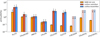Fig. 13

Ratio of complex organic molecules with respect to CH₃OH in S68N. The ratios are shown for a 3′′ region in the red- and blueshifted part of the outflow. The abundance ratios in the hot cores are taken from van Gelder et al. (2020) and Nazari et al. (2021). The error bars mark the lower and upper limit on the ratios, as calculated from the optically thick CH₃OH emission (lower limit) and ¹³CH₃OH (upper limit). All outflow abundances obtained from the band 6 data are at 0.′′45 resolution, except for CH₃OCHO and CH₃CN, which were derived from band 3 data at 3′′ resolution.

4.6 Carbon chains and other hydrocarbons versus COMs

Early observations at low spatial resolution suggested that large carbon chains such as C₅H, HC₇N, and HC₉N and complex organic molecules are mutually exclusive, and therefore the two were proposed to be tracers of two different categories of protostellar sources driven by different chemistry, namely warm carbon-chain chemistry (WCCC) and hot-core chemistry (Sakai & Yamamoto 2013). Warm carbon-chain chemistry is thought to occur above the sublimation temperature of CH₄ ~ at 30 K. The proposed difference then lies in the WCCC sources, which collapse more rapidly than the hot-core sources, which prevents CO from accumulating on the ices, leaving a higher CH₄ ice content. Thus, in WCCC sources, there would be less CO to form more complex organic molecules such as CH₃OH, and an underabundance of COMs is indeed observed. This scenario has been supported by the lower deuteration observed in WCCC sources (Sakai et al. 2009). With ALMA observations at higher resolution and sensitivity, sources harboring both COMs and small hydrocarbons, c-C₃H₂, and C₂H, have now been observed (Imai et al. 2016; Oya et al. 2017).

Our data also show detections of small hydrocarbons and COMs in the same sources (Fig. 14). However, our high-resolution maps now show that these hydrocarbons originate in the UV-irradiated outflow cavity walls (Sect. 4.3). Both c-C₃H₂ and C₂H can be explained by PDR chemistry alone (Guzmán et al. 2015; Cuadrado et al. 2015) even in moderate UV fields of low-mass protostars, and therefore WCCC chemistry does not need to be invoked for the sources presented in this work. The PDR origin is consistent with our observed geometry at the edges of the cavities, where lower extinction allows the UV radiation from the protostellar accretion to easily reach this region. It also explains the confinement of this emission to the inner 2000 au of the envelope as the UV radiation decreases with distance from the source. A deep search for larger hydrocarbons such as HC₅N in cavity walls could help to understand their origin.

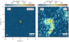Fig. 14

Emission maps of an example COM and hydrocarbon toward B1-c. Left: CH₃CHO moment 0 map. Right: C₂H moment 0 map. Both are integrated from −2 to 2 km s⁻¹ with respect to v_sys.

4.7 Class 0 versus Class I in different components

Many processes take place within the protostellar lifetime of a few 10⁵ yr and alter the chemical composition and physical conditions. First, the envelope dissipates, and the radius within which key molecules are in the gas phase decreases (Jørgensen et al. 2005b). With high-resolution studies, it is now possible to probe different snow lines in unprecedented detail (van ’t Hoff et al. 2018a; Hsieh et al. 2019). A clear evolutionary trend is observed in temperature: Class 0 disks are generally warmer than Class II disks, and Class I sources are in between. This has a strong effect on therichness of their spectra (van ’t Hoff et al. 2020a,b). This is also observed in our sample, where all Class 0 sources show either complex organic molecules or small molecules related to grain evaporation, but no evidence of these molecules is found in Class I sources (Sect. 4.4.1). Table 3 summarizes the evolution of the molecular composition of protostellar systems.

Complex organic molecules are a key tracer of chemistry at the early stages. We detect them in the outflows only in Class 0 sources, probably because the outflow force, mass, and envelope density decrease. In the inner regions, physical conditions such as temperatureand density also favor the early stages for the abundances of COMs. In the rare cases of a rich chemistry in Class I disks, it is usually attributed to accretion outbursts heating up the disk (van ’t Hoff et al. 2018c; Lee et al. 2019a).

Molecular EHV jets are only present in the Class 0 phase (Nisini et al. 2015). In our sample, six out of seven sources have a high-velocity component, and none is detected in Class I (Sect. 4.2.1), whereas the lower-velocity outflows in these stages are rich in ice-mantle tracers (Sect. 4.2.3). The Class I jets are invisible in molecular tracers, and their outflows primarily show CO, with a far weaker contribution from shock tracers such as SO and SiO (Sect. 4.2.2).

Cavity walls are observed prominently in the Class 0 sources in molecules whose abundances are sensitive to UV radiation. In Class I sources, a flared disk and weak outflow remain. While there is less envelope material to attenuate the UV radiation, there is also less material to irradiate and the accretion luminosity of older sources decreases, which results in less prominent emission from UV tracers on large scales in Class I (Sect. 4.3). Another example of a transition of the molecular appearance between Class 0 and I is SO: this molecule primarily traces the outflow in Class 0 and the disk-envelope interface in Class I.

Table 3

Summary of evolution of chemical tracers.

5 Conclusions

We have presented an overview of the molecular tracers of the physical components in protostellar Class 0 and Class I systems. Table 2 and Fig. 11 present an overview of the results, which are summarized below.

Protostellar envelopes are primarily traced with dense-gas tracers such as C¹⁸O and CO, and snow-line tracers such as DCO⁺, N₂D⁺, and H¹³CO⁺. For this component, it is essential to use observations that are sensitive to large scales of ~5000 au.
Protostellar outflows are separated into different components. High-velocity molecular jets are traced by the O-bearing molecules CO, SiO, SO, and H₂CO. Entrained outflow material can be probed by low-velocity CO, SiO, SO, H₂CO, and HCN as well as by molecules released from ices by sputtering, such as CH₃OH, CH₃CHO, HNCO, CH₃CN, and CH₃OCHO.
Outflow cavity walls are pronounced in UV irradiation tracers: C₂H, c-C₃H₂, and CN, and high-density tracers such as ¹³CS.
Hot cores, the inner warm envelopes, are probed predominantly by COMs and simple molecules released from ice mantles and produced by high-temperature chemistry such as SO, H₂S, H₂CS, OCS, H¹³CN, HCOOH, and HNCO.
Embedded disks, which are most clearly detected in Class I sources, can be observed in C¹⁷O and H₂CO, while CN traces their upper layers. CO isotopologs can be used to probe disks in Class 0 sources. However, the confusion with the envelope emission requires a detailed analysis of the kinematics to confirm that a Keplerian disk is present.

Hydrocarbons and COMs are found to coexist routinely in protostellar sources: the first are present in the UV-irradiated cavity walls, and COMs are present in the hot core and in the outflows. It is plausible that PDR chemistry for the formation of hydrocarbons is sufficient to explain the presence of molecules such as C₂H and c-C₃H₂, and that no warm carbon-chain chemistry is required, which relies on abundant CH₄ in ices. Observations of more complex carbon chains in cavity walls and envelopes are necessary to understand whether the WCCC plays a role there. The JWST will be able to probe the CH₄ ice content at spatial scales comparable to ALMA, which will show if there are any differences in the ice composition between sources.

Throughout this study, the availability of low-lying molecular lines to probe the cold extended envelope and outflow and high-excitation lines to trace compact hot cores was key for the analysis. The occurrence of the same molecules in different physical components provides an opportunity to study the processes involved in their formation and excitation. For example, ice-mantle tracers sputtered from the grains in outflows give useful insight into the ice composition, whereas a comparison with abundances of thermally released COMs in the inner region is a powerful tool to probe whether gas-phase formation routes contribute to complex molecule formation.

JWST-MIRI will provide unprecedented resolution and sensitivity in the mid-IR that will allow probing the emission from hot gas in shocks and ice-absorption features. JWST observations can then be combined with our understanding of the kinematics and spatial origin of molecules revealed by ALMA.

Acknowledgements

The authors are grateful to the anonymous referee for comments that improved the quality of the paper. This paper makes use of the following ALMA data: ADS/JAO.ALMA# 2017.1.01174.S, ADS/JAO.ALMA# 2017.1.01350.S, ADS/JAO.ALMA# 2017.1.01371.S, ADS/JAO.ALMA# 2017.1. 01413.S, ADS/JAO.ALMA# 2013.1.00726.S, ADS/JAO.ALMA# 2016.1.00710.S. ALMA is a partnership of ESO (representing its member states), NSF (USA) and NINS (Japan), together with NRC (Canada), MOST and ASIAA (Taiwan), and KASI (Republic of Korea), in co-operation with the Republic of Chile. The Joint ALMA Observatory is operated by ESO, AUI/NRAO and NAOJ. Astrochemistry in Leiden is supported by the Netherlands Research School for Astronomy (NOVA). Ł.T. acknowledges the ESO Fellowship Programme. M.L.vG. acknowledges support from the Dutch Research Council (NWO) with projectnumber NWO TOP-1 614.001.751. C.L.H.H. acknowledges the support of the NAOJ Fellowship and JSPS KAKENHI grants 18K13586 and 20K14527. The National Radio Astronomy Observatory is a facility of the National Science Foundation operated under cooperative agreement by Associated Universities, Inc. This research has made use of NASA’s Astrophysics Data System Bibliographic Services. This research made use of NumPy (Harris et al. 2020); Astroquery (Ginsburg et al. 2019); Astropy, a community-developed core Python package for Astronomy (Astropy Collaboration 2018, 2013); Pandas (McKinney 2010, 2011); and Matplotlib (Hunter 2007).

Appendix A Tables

Table A.1

Specifications of observations

Table A.2

Molecular transitions targeted

Appendix B Continuum images

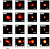Fig. B.1

Continuum emission from the sources in the sample.

Appendix C Envelope tracers

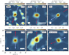Fig. C.1

Moment maps of C¹⁸O 2–1 (E_up=16 K) at 6′′ resolution. Contours: Continuum. Color scale: C¹⁸O integrated from -2 to 2 km s⁻¹ with respect to v_sys.

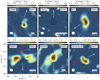Fig. C.2

Moment maps of N₂D⁺ 3–2 (E_up=22 K) at 6′′ resolution. Contours: Continuum. Color scale: Moment-0 map integrated from -2 to 2 km s⁻¹ with respect to v_sys.

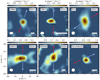Fig. C.3

Moment maps of DCO⁺ 3–2 (E_up=21 K) at 6′′ resolution. Contours: Continuum. Color scale: Moment-0 map integrated from -2 to 2 km s⁻¹ with respect to v_sys.

Appendix D Outflow

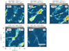Fig. D.1

Moment maps of low-velocity CO 2–1 (E_up=17 K) outflow at 0.′′4 resolution. Contours: Continuum. Color scale: Moment-0 map integrated from -10 to 10 km s⁻¹ with respect to v_sys.

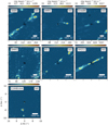Fig. D.2

Moment maps of low-velocity SiO 5–4 (E_up =34 K) and 4–3 (E_up =21 K) outflow at 0.′′4 resolution. Contours: Continuum. Color scale: Moment-0 map integrated from -15 to 15 km s⁻¹ with respect to v_sys.

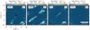Fig. D.3

Moment maps of low-velocity SO 5₆–4₅ (E_up =35 K) and 6₇–5₆ (E_up =48 K) outflow at 0.′′4 resolution. Contours: Continuum. Color scale: Moment 0 map integrated from -10 to 10 km s⁻¹ with respect to v_sys.

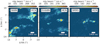Fig. D.4

Moment maps of HCN 1–0 (E_up=4 K) at 0.′′5 resolution. Color scale: Moment-0 map integrated from -15 to 15 km s⁻¹ with respect to v_sys.

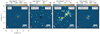Fig. D.5

Moment maps of H¹³CN 2–1 (E_up=14 K) at 0.′′4 resolution. Contours: Continuum. Color scale: Moment-0 map integrated from -7 to 7 km s⁻¹ with respect to v_sys.

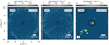Fig. D.6

Additional plots of sputtering products for S68N. CH₃CHO 14_0,14 –13_0,13(E_up = 96 K) and H₂CCO 13_1,13 –12_1,12 (E_up =101 K), which are separated by 4 km s⁻¹, and CH₃OCHO 10_0,10 –9_0,9 (E_up =30 K).

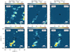Fig. D.7

Moment-0 map in color scale and 1.3 mm continuum in contours of SMM3. CO 2–1 (E_up =17 K), H₂CO 3_2,1 -2_2,0 E_up = 68 K, and CH₃OH 4₂ –5₁ E_up =60 K moment-0 maps obtained in band 6 at 0.′′5 resolution. CH₃CHO 6_1,6,1 –5_1,5,1 E_up =21 K, HNCO 5_0,5–4_0,4 E_up =16 K, CH₃CN 6₀ –5₀ E_up =19 K, and CH₃OCHO 9_5,5 –8_5,4 E_up =43 K. Map of the sputtering product emission toward SMM3 in band 3 at 3′′ resolution. Moment-0 map integrated from -4 to 4 km s⁻¹ with respect to - v_sys.

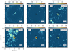Fig. D.8

Moment-0 map in color scale and 1.3 mm continuum in contours of B1-c. CO 2–1 E_up =48 K and CH₃OH 4₂ –5₁ E_up =60 K moment-0 maps obtained in band 6 at 0.′′5 resolution. Sputtering product emission toward SMM3 in band 3 at 3′′ resolution. CH₃CHO 6_1,6,1 –5_1,5,1 E_up =21 K, HNCO 5_0,5–4_0,4 E_up =16 K, and CH₃CN 6₀ -5₀ E_up =19 K and CH₃OCHO 9_5,5 –8_5,4 E_up =43 K. Moment-0 map integrated from -10 to 10 km s⁻¹ with respect to v_sys for SO and from -2 to 2 km s⁻¹ with respect to v_sys for the other molecules.

Appendix E Cavity walls

Fig. E.1

Maps of the outflow cavity wall tracers toward S68N, TMC1, and Emb8N with the CO low-velocity outflow map for reference. Top: Moment-0 maps toward S68N of CO and C₂H, H¹³CO⁺ obtained in band 6 at 0.′′5 resolution and CN in band 3 at 3′′. Middle: Moment-0 maps toward TMC1 of CO, c-C₃H₂, and ¹³CS and CN obtained at 0.′′5. The emission is integrated from -5 to -1 km s⁻¹ and from 1 to 5 km s⁻¹ with respec to v_sys. Bottom: Moment-0 maps toward Emb8N of CO, c-C₂H, and H¹³CO⁺ ¹³CS at 0.′′5 in band 6. and CN in band 3 at 3′′. The emission is integrated from -5 to 5 km s⁻¹ with respect to v_sys.

Fig. E.2

¹³CS 5–4 (E_up =33 K) integrated from -5 to 5 km s⁻¹ with respect to v_sys in band 6 at 0.′′5.

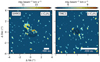Fig. E.3

c-C₃H₂ 7_2,6 –7_1,7 (E_up =63 K) integrated from -1.5 to 1.5 km s⁻¹ with respect to v_sys.

Appendix F Inner envelope

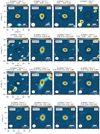Fig. F.1

CCS 19₁₈–18₁₇ E_up =111 K, OCS 19–18 E_up=111 K, and H₂CO 9_1,8 –9_1,9 E_up =174 K, H₂S 2₂ –2₁ E_up =83 K moment-0 maps from ACA band 6 observations and 6′′ resolution integrated from -2 to 2 km s⁻¹ with respect to v_sys.

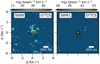Fig. F.2

O¹³CS 18–17 E_up=99 K integratedfrom -3 to 3 km s⁻¹ with respect to v_sys.

Appendix G Additional plots

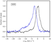Fig. G.1

Spectra of SO 6₇–5₆ for S68N. Spectra averaged over the 0.′′6 diameter circle on positions of the central source (black) and the blueshifted outflow (blue). Both spectra normalized to the peak emission at the position.

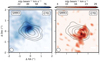Fig. G.2

Map of the C¹⁸O emission toward SMM3. Moment-0 map in color scale and 1.3 mm continuum in contours. Left: Moment-0 map integrated from -3 to -0.5 km s⁻¹ with respect to v_sys. Right: Moment-0 map integrated from 0.5 to 3 km s⁻¹ with respect to v_sys.

References

Abergel, A., Teyssier, D., Bernard, J. P., et al. 2003, A&A, 410, 577 [NASA ADS] [CrossRef] [EDP Sciences] [Google Scholar]
ALMA Partnership (Brogan, C. L., et al.) 2015, ApJ, 808, L3 [Google Scholar]
Anderl, S., Maret, S., Cabrit, S., et al. 2016, A&A, 591, A3 [NASA ADS] [CrossRef] [EDP Sciences] [Google Scholar]
André, P., Ward-Thompson, D., & Barsony, M. 1993, ApJ, 406, 122 [Google Scholar]
Arce, H. G., & Sargent, A. I. 2006, ApJ, 646, 1070 [NASA ADS] [CrossRef] [Google Scholar]
Arce, H. G., Santiago-García, J., Jørgensen, J. K., Tafalla, M., & Bachiller, R. 2008, ApJ, 681, L21 [NASA ADS] [CrossRef] [Google Scholar]
Artur de la Villarmois, E., Jørgensen, J. K., Kristensen, L. E., et al. 2019, A&A, 626, A71 [NASA ADS] [CrossRef] [EDP Sciences] [Google Scholar]
Astropy Collaboration (Robitaille, T. P., et al.) 2013, A&A, 558, A33 [NASA ADS] [CrossRef] [EDP Sciences] [Google Scholar]
Astropy Collaboration (Price-Whelan, A. M., et al.) 2018, AJ, 156, 123 [Google Scholar]
Bachiller, R., & Gomez-Gonzalez, J. 1992, A&ARv, 3, 257 [NASA ADS] [CrossRef] [Google Scholar]
Bacmann, A., Taquet, V., Faure, A., Kahane, C., & Ceccarelli, C. 2012, A&A, 541, L12 [NASA ADS] [CrossRef] [EDP Sciences] [Google Scholar]
Belloche, A., Maury, A. J., Maret, S., et al. 2020, A&A, 635, A198 [NASA ADS] [CrossRef] [EDP Sciences] [Google Scholar]
Benz, A. O., Bruderer, S., van Dishoeck, E. F., et al. 2016, A&A, 590, A105 [NASA ADS] [CrossRef] [EDP Sciences] [Google Scholar]
Bergner, J. B., Öberg, K. I., Garrod, R. T., & Graninger, D. M. 2017, ApJ, 841, 120 [Google Scholar]
Bergner, J. B., Öberg, K. I., Walker, S., et al. 2019, ApJ, 884, L36 [CrossRef] [Google Scholar]
Bianchi, E., Chandler, C. J., Ceccarelli, C., et al. 2020, MNRAS, 498, L87 [NASA ADS] [CrossRef] [Google Scholar]
Bjerkeli, P., van der Wiel, M. H. D., Harsono, D., Ramsey, J. P., & Jørgensen, J. K. 2016, Nature, 540, 406 [Google Scholar]
Bontemps, S., Andre, P., Terebey, S., & Cabrit, S. 1996, A&A, 311, 858 [NASA ADS] [Google Scholar]
Boogert, A. C. A., Gerakines, P. A., & Whittet, D. C. B. 2015, ARA&A, 53, 541 [Google Scholar]
Bruderer, S., Benz, A. O., Bourke, T. L., & Doty, S. D. 2009, A&A, 503, L13 [NASA ADS] [CrossRef] [EDP Sciences] [Google Scholar]
Buckle, J. V., & Fuller, G. A. 2002, A&A, 381, 77 [NASA ADS] [CrossRef] [EDP Sciences] [Google Scholar]
Burkhardt, A. M., Dollhopf, N. M., Corby, J. F., et al. 2016, ApJ, 827, 21 [CrossRef] [Google Scholar]
Cabrit, S., & Bertout, C. 1992, A&A, 261, 274 [Google Scholar]
Carney, M. T., Fedele, D., Hogerheijde, M. R., et al. 2018, A&A, 614, A106 [NASA ADS] [CrossRef] [EDP Sciences] [Google Scholar]
Caselli, P., & Ceccarelli, C. 2012, A&ARv, 20, 56 [Google Scholar]
Caselli, P., Hartquist, T. W., & Havnes, O. 1997, A&A, 322, 296 [NASA ADS] [Google Scholar]
Caselli, P., Walmsley, C. M., Tafalla, M., Dore, L., & Myers, P. C. 1999, ApJ, 523, L165 [Google Scholar]
Caselli, P., Keto, E., Bergin, E. A., et al. 2012, ApJ, 759, L37 [Google Scholar]
Cassen, P., & Moosman, A. 1981, Icarus, 48, 353 [CrossRef] [Google Scholar]
Ceccarelli, C., Caselli, P., Fontani, F., et al. 2017, ApJ, 850, 176 [NASA ADS] [CrossRef] [Google Scholar]
Chandler, C. J., & Carlstrom, J. E. 1996, ApJ, 466, 338 [Google Scholar]
Chen, H., Myers, P. C., Ladd, E. F., & Wood, D. O. S. 1995, ApJ, 445, 377 [NASA ADS] [CrossRef] [Google Scholar]
Chen, X., Launhardt, R., & Henning, T. 2007, ApJ, 669, 1058 [NASA ADS] [CrossRef] [Google Scholar]
Codella, C., Ceccarelli, C., Nisini, B., et al. 2010, A&A, 522, L1 [NASA ADS] [CrossRef] [EDP Sciences] [Google Scholar]
Codella, C., Ceccarelli, C., Caselli, P., et al. 2017, A&A, 605, L3 [NASA ADS] [CrossRef] [EDP Sciences] [Google Scholar]
Codella, C., Bianchi, E., Tabone, B., et al. 2018, A&A, 617, A10 [NASA ADS] [CrossRef] [EDP Sciences] [Google Scholar]
Codella, C., Ceccarelli, C., Bianchi, E., et al. 2020, A&A, 635, A17 [NASA ADS] [CrossRef] [EDP Sciences] [Google Scholar]
Crapsi, A., van Dishoeck, E. F., Hogerheijde, M. R., Pontoppidan, K. M., & Dullemond, C. P. 2008, A&A, 486, 245 [NASA ADS] [CrossRef] [EDP Sciences] [Google Scholar]
Cuadrado, S., Goicoechea, J. R., Pilleri, P., et al. 2015, A&A, 575, A82 [NASA ADS] [CrossRef] [EDP Sciences] [Google Scholar]
De Simone, M., Ceccarelli, C., Codella, C., et al. 2020a, ApJ, 896, L3 [NASA ADS] [CrossRef] [Google Scholar]
De Simone, M., Codella, C., Ceccarelli, C., et al. 2020b, A&A, 640, A75 [NASA ADS] [CrossRef] [EDP Sciences] [Google Scholar]
Draine, B. T. 1978, ApJS, 36, 595 [Google Scholar]
Drozdovskaya,M. N., van Dishoeck, E. F., Jørgensen, J. K., et al. 2018, MNRAS, 476, 4949 [NASA ADS] [CrossRef] [Google Scholar]
Dutrey, A., Guilloteau, S., & Bachiller, R. 1997, A&A, 325, 758 [NASA ADS] [Google Scholar]
Emprechtinger, M., Caselli, P., Volgenau, N. H., Stutzki, J., & Wiedner, M. C. 2009, A&A, 493, 89 [NASA ADS] [CrossRef] [EDP Sciences] [Google Scholar]
Enoch, M. L., Evans, II, N. J., Sargent, A. I., & Glenn, J. 2009, ApJ, 692, 973 [Google Scholar]
Evans, Neal J., I. 1999, ARA&A, 37, 311 [NASA ADS] [CrossRef] [Google Scholar]
Favre, C., Bergin, E. A., Cleeves, L. I., et al. 2015, ApJ, 802, L23 [NASA ADS] [CrossRef] [Google Scholar]
Flower, D. R., & Pineau des Forêts, G. 2013, MNRAS, 436, 2143 [NASA ADS] [CrossRef] [Google Scholar]
Frimann, S., Jørgensen, J. K., Dunham, M. M., et al. 2017, A&A, 602, A120 [NASA ADS] [CrossRef] [EDP Sciences] [Google Scholar]
Fuente, A., Martin-Pintado, J., Cernicharo, J., & Bachiller, R. 1993, A&A, 276, 473 [NASA ADS] [Google Scholar]
Garufi, A., Podio, L., Codella, C., et al. 2021, A&A, 645, A145 [EDP Sciences] [Google Scholar]
Geers, V. C., van Dishoeck, E. F., Pontoppidan, K. M., et al. 2009, A&A, 495, 837 [NASA ADS] [CrossRef] [EDP Sciences] [Google Scholar]
Ginsburg, A., Sipőcz, B. M., Brasseur, C. E., et al. 2019, AJ, 157, 98 [Google Scholar]
Glassgold, A. E., Mamon, G. A., & Huggins, P. J. 1991, ApJ, 373, 254 [NASA ADS] [CrossRef] [Google Scholar]
Greaves, J. S., & Rice, W. K. M. 2010, MNRAS, 407, 1981 [CrossRef] [Google Scholar]
Green, J. D., Evans, II, N. J., Jørgensen, J. K., et al. 2013, ApJ, 770, 123 [NASA ADS] [CrossRef] [Google Scholar]
Greene, T. P., Meyer, M. R., Ressler, M. E., Rieke, M. J., & Van Dishoeck, E. F. 2017, Protostar (YSO) Spectroscopy (USA: JWST Proposal, Cycle1), 1186 [Google Scholar]
Gueth, F., & Guilloteau, S. 1999, A&A, 343, 571 [NASA ADS] [Google Scholar]
Gueth, F., Guilloteau, S., & Bachiller, R. 1996, A&A, 307, 891 [NASA ADS] [Google Scholar]
Guilloteau, S., Bachiller, R., Fuente, A., & Lucas, R. 1992, A&A, 265, L49 [NASA ADS] [Google Scholar]
Gusdorf, A., Cabrit, S., Flower, D. R., & Pineau des Forêts, G. 2008a, A&A, 482, 809 [NASA ADS] [CrossRef] [EDP Sciences] [Google Scholar]
Gusdorf, A., Pineau des Forêts, G., Cabrit, S., & Flower, D. R. 2008b, A&A, 490, 695 [NASA ADS] [CrossRef] [EDP Sciences] [Google Scholar]
Guzmán, V. V., Pety, J., Goicoechea, J. R., et al. 2015, ApJ, 800, L33 [CrossRef] [Google Scholar]
Harris, C. R., Millman, K. J., van der Walt, S. J., et al. 2020, Nature, 585, 357 [NASA ADS] [CrossRef] [Google Scholar]
Harsono, D., Jørgensen, J. K., van Dishoeck, E. F., et al. 2014, A&A, 562, A77 [NASA ADS] [CrossRef] [EDP Sciences] [Google Scholar]
Harsono, D., Bruderer, S., & van Dishoeck, E. F. 2015a, A&A, 582, A41 [NASA ADS] [CrossRef] [EDP Sciences] [Google Scholar]
Harsono, D., van Dishoeck, E. F., Bruderer, S., Li, Z. Y., & Jørgensen, J. K. 2015b, A&A, 577, A22 [NASA ADS] [CrossRef] [EDP Sciences] [Google Scholar]
Harsono, D., Bjerkeli, P., van der Wiel, M. H. D., et al. 2018, Nat. Astron., 2, 646 [Google Scholar]
Harsono, D., van der Wiel, M. H. D., Bjerkeli, P., et al. 2021, A&A, 646, A72 [NASA ADS] [CrossRef] [EDP Sciences] [Google Scholar]
Harsono, D., Bjerkeli, P., Jorgensen, J., et al. 2021, Mapping the Hot Gas where an Outflow is Launched from a Protoplanetary Disk (USA: JWST Proposal, Cycle 1), 2104 [Google Scholar]
Hartquist, T. W., Dalgarno, A., & Oppenheimer, M. 1980, ApJ, 236, 182 [NASA ADS] [CrossRef] [Google Scholar]
Herbst, E., & van Dishoeck, E. F. 2009, Ann. Rev. Astron. Astrophys., 47, 427 [Google Scholar]
Hernández-Gómez, A., Sahnoun, E., Caux, E., et al. 2018, MNRAS, 483, 2014 [Google Scholar]
Hogerheijde, M. R., Jansen, D. J., & van Dishoeck, E. F. 1995, A&A, 294, 792 [NASA ADS] [Google Scholar]
Hogerheijde, M. R., van Dishoeck, E. F., Blake, G. A., & van Langevelde, H. J. 1997, ApJ, 489, 293 [NASA ADS] [CrossRef] [Google Scholar]
Hogerheijde, M. R., van Dishoeck, E. F., Salverda, J. M., & Blake, G. A. 1999, ApJ, 513, 350 [NASA ADS] [CrossRef] [Google Scholar]
Hollenbach, D. J., & Tielens, A. G. G. M. 1997, ARA&A, 35, 179 [NASA ADS] [CrossRef] [Google Scholar]
Hsieh, T.-H., Murillo, N. M., Belloche, A., et al. 2019, ApJ, 884, 149 [Google Scholar]
Hueso, R., & Guillot, T. 2005, A&A, 442, 703 [NASA ADS] [CrossRef] [EDP Sciences] [Google Scholar]
Hull, C. L. H., Girart, J. M., Kristensen, L. E., et al. 2016, ApJ, 823, L27 [CrossRef] [Google Scholar]
Hull, C. L. H., Girart, J. M., Tychoniec, Ł., et al. 2017, ApJ, 847, 92 [NASA ADS] [CrossRef] [Google Scholar]
Hunter, J. D. 2007, Comput. Sci. Eng., 9, 90 [NASA ADS] [CrossRef] [Google Scholar]
Imai, M., Sakai, N., Oya, Y., et al. 2016, ApJ, 830, L37 [CrossRef] [Google Scholar]
Ivezic, Z., & Elitzur, M. 1997, MNRAS, 287, 799 [Google Scholar]
Jansen, D. J., Spaans, M., Hogerheijde, M. R., & van Dishoeck, E. F. 1995, A&A, 303, 541 [NASA ADS] [Google Scholar]
Jiménez-Serra, I., Caselli, P., Martín-Pintado, J., & Hartquist, T. W. 2008, A&A, 482, 549 [NASA ADS] [CrossRef] [EDP Sciences] [Google Scholar]
Jørgensen, J. K., Schöier, F. L., & van Dishoeck, E. F. 2002, A&A, 389, 908 [CrossRef] [EDP Sciences] [Google Scholar]
Jørgensen, J. K., Schöier, F. L., & van Dishoeck, E. F. 2004a, A&A, 416, 603 [Google Scholar]
Jørgensen, J. K., Hogerheijde, M. R., Blake, G. A., et al. 2004b, A&A, 415, 1021 [NASA ADS] [CrossRef] [EDP Sciences] [Google Scholar]
Jørgensen, J. K., Bourke, T. L., Myers, P. C., et al. 2005a, ApJ, 632, 973 [Google Scholar]
Jørgensen, J. K., Schöier, F. L., & van Dishoeck, E. F. 2005b, A&A, 435, 177 [NASA ADS] [CrossRef] [EDP Sciences] [Google Scholar]
Jørgensen, J. K., Johnstone, D., Kirk, H., & Myers, P. C. 2007, ApJ, 656, 293 [Google Scholar]
Jørgensen, J. K., van Dishoeck, E. F., Visser, R., et al. 2009, A&A, 507, 861 [NASA ADS] [CrossRef] [EDP Sciences] [Google Scholar]
Jørgensen, J. K., Visser, R., Sakai, N., et al. 2013, ApJ, 779, L22 [Google Scholar]
Jørgensen, J. K., Visser, R., Williams, J. P., & Bergin, E. A. 2015, A&A, 579, A23 [NASA ADS] [CrossRef] [EDP Sciences] [Google Scholar]
Jørgensen, J. K., van der Wiel, M. H. D., Coutens, A., et al. 2016, A&A, 595, A117 [Google Scholar]
Karska, A., Kaufman, M. J., Kristensen, L. E., et al. 2018, ApJS, 235, 30 [NASA ADS] [CrossRef] [Google Scholar]
Kristensen, L. E., van Dishoeck, E. F., Bergin, E. A., et al. 2012, A&A, 542, A8 [NASA ADS] [CrossRef] [EDP Sciences] [Google Scholar]
Lada, C. J. 1987, IAU Symp., 115, 1 [Google Scholar]
Le Gouellec, V. J. M., Hull, C. L. H., Maury, A. J., et al. 2019, ApJ, 885, 106 [NASA ADS] [CrossRef] [Google Scholar]
Lee, C.-F. 2020, A&ARv, 28, 1 [NASA ADS] [CrossRef] [Google Scholar]
Lee, C.-F., Ho, P. T. P., Palau, A., et al. 2007, ApJ, 670, 1188 [NASA ADS] [CrossRef] [Google Scholar]
Lee, C.-F., Hirano, N., Zhang, Q., et al. 2014, ApJ, 786, 114 [NASA ADS] [CrossRef] [Google Scholar]
Lee, C.-F., Hirano, N., Zhang, Q., et al. 2015, ApJ, 805, 186 [NASA ADS] [CrossRef] [Google Scholar]
Lee, C.-F., Codella, C., Li, Z.-Y., & Liu, S.-Y. 2019a, ApJ, 876, 63 [Google Scholar]
Lee, J.-E., Lee, S., Baek, G., et al. 2019b, Nat. Astron., 3, 314 [Google Scholar]
López-Sepulcre, A., Sakai, N., Neri, R., et al. 2017, A&A, 606, A121 [NASA ADS] [CrossRef] [EDP Sciences] [Google Scholar]
Machida, M. N., Matsumoto, T., & Inutsuka, S.-i. 2016, MNRAS, 463, 4246 [Google Scholar]
Manara, C. F., Morbidelli, A., & Guillot, T. 2018, A&A, 618, L3 [NASA ADS] [CrossRef] [EDP Sciences] [Google Scholar]
Manigand, S., Jørgensen, J. K., Calcutt, H., et al. 2020, A&A, 635, A48 [NASA ADS] [CrossRef] [EDP Sciences] [Google Scholar]
Marconi, A., Testi, L., Natta, A., & Walmsley, C. M. 1998, A&A, 330, 696 [NASA ADS] [Google Scholar]
Maret, S., Maury, A. J., Belloche, A., et al. 2020, A&A, 635, A15 [NASA ADS] [CrossRef] [EDP Sciences] [Google Scholar]
Mathews, G. S., Klaassen, P. D., Juhász, A., et al. 2013, A&A, 557, A132 [NASA ADS] [CrossRef] [EDP Sciences] [Google Scholar]
Maury, A. J., André, P., Men’shchikov, A., Könyves, V., & Bontemps, S. 2011, A&A, 535, A77 [NASA ADS] [CrossRef] [EDP Sciences] [Google Scholar]
Maury, A. J., André, P., Testi, L., et al. 2019, A&A, 621, A76 [NASA ADS] [CrossRef] [EDP Sciences] [Google Scholar]
McClure, M. K. 2019, A&A, 632, A32 [NASA ADS] [CrossRef] [EDP Sciences] [Google Scholar]
McKinney, W. 2010, in Proceedings of the 9th Python in Science Conference, Vol. 445, Austin, TX, 51–56 [Google Scholar]
McKinney, W. 2011, Python for High Performance and Scientific Computing, 14 [Google Scholar]
Milam, S. N., Savage, C., Brewster, M. A., Ziurys, L. M., & Wyckoff, S. 2005, ApJ, 634, 1126 [Google Scholar]
Millar, T. J., & Williams, D. A. 1993, Dust and Chemistry in Astronomy (Bristol: IOP Publishing) [Google Scholar]
Mottram, J. C., van Dishoeck, E. F., Kristensen, L. E., et al. 2017, A&A, 600, A99 [NASA ADS] [CrossRef] [EDP Sciences] [Google Scholar]
Murillo, N. M., Lai, S.-P., Bruderer, S., Harsono, D., & van Dishoeck, E. F. 2013, A&A, 560, A103 [NASA ADS] [CrossRef] [EDP Sciences] [Google Scholar]
Murillo, N. M., Bruderer, S., van Dishoeck, E. F., et al. 2015, A&A, 579, A114 [NASA ADS] [CrossRef] [EDP Sciences] [Google Scholar]
Navarro-Almaida, D., Le Gal, R., Fuente, A., et al. 2020, A&A, 637, A39 [NASA ADS] [CrossRef] [EDP Sciences] [Google Scholar]
Nazari, P., van Gelder, M. L., van Dishoeck, E. F., et al. 2021, A&A, 650, A150 [EDP Sciences] [Google Scholar]
Nisini, B., Santangelo, G., Giannini, T., et al. 2015, ApJ, 801, 121 [NASA ADS] [CrossRef] [Google Scholar]
Öberg, K. I., Garrod, R. T., van Dishoeck, E. F., & Linnartz, H. 2009, A&A, 504, 891 [NASA ADS] [CrossRef] [EDP Sciences] [Google Scholar]
Offner, S. S. R., & Arce, H. G. 2014, ApJ, 784, 61 [NASA ADS] [CrossRef] [Google Scholar]
Ohashi, N., Saigo, K., Aso, Y., et al. 2014, ApJ, 796, 131 [NASA ADS] [CrossRef] [Google Scholar]
Oya, Y., Sakai, N., Watanabe, Y., et al. 2017, ApJ, 837, 174 [Google Scholar]
Perotti, G., Rocha, W. R. M., Jørgensen, J. K., et al. 2020, A&A, 643, A48 [EDP Sciences] [Google Scholar]
Pety, J., Teyssier, D., Fossé, D., et al. 2005, A&A, 435, 885 [NASA ADS] [CrossRef] [EDP Sciences] [Google Scholar]
Pety, J., Gratier, P., Guzmán, V., et al. 2012, A&A, 548, A68 [NASA ADS] [CrossRef] [EDP Sciences] [Google Scholar]
Pineda, J. E., Zhao, B., Schmiedeke, A., et al. 2019, ApJ, 882, 103 [NASA ADS] [CrossRef] [Google Scholar]
Pineda, J. E., Segura-Cox, D., Caselli, P., et al. 2020, Nat. Astron., 4, 1158 [NASA ADS] [CrossRef] [Google Scholar]
Podio, L., Codella, C., Gueth, F., et al. 2015, A&A, 581, A85 [NASA ADS] [CrossRef] [EDP Sciences] [Google Scholar]
Podio, L., Garufi, A., Codella, C., et al. 2020, A&A, 642, L7 [NASA ADS] [CrossRef] [EDP Sciences] [Google Scholar]
Podio, L., Tabone, B., Codella, C., et al. 2021, A&A, 648, A45 [NASA ADS] [CrossRef] [EDP Sciences] [Google Scholar]
Qi, C., Öberg, K. I., Andrews, S. M., et al. 2015, ApJ, 813, 128 [Google Scholar]
Raga, A. C., Canto, J., Binette, L., & Calvet, N. 1990, ApJ, 364, 601 [NASA ADS] [CrossRef] [Google Scholar]
Raga, A. C., Williams, D. A., & Lim, A. J. 2005, Rev. Mex. Astron. Astrofis., 41, 137 [Google Scholar]
Ray, T. P., Beuther, H., Caratti o Garatti, A., et al. 2017, The Young Protostellar Outflow HH211, (USA: JWST Proposal, Cycle 1) 1257 [Google Scholar]
Rodríguez-Fernández, N. J., Tafalla, M., Gueth, F., & Bachiller, R. 2010, A&A, 516, A98 [Google Scholar]
Sakai, N., & Yamamoto, S. 2013, Chem. Rev., 113, 8981 [Google Scholar]
Sakai, N., Sakai, T., Hirota, T., Burton, M., & Yamamoto, S. 2009, ApJ, 697, 769 [Google Scholar]
Sakai, N., Ceccarelli, C., Bottinelli, S., Sakai, T., & Yamamoto, S. 2012, ApJ, 754, 70 [NASA ADS] [CrossRef] [Google Scholar]
Sakai, N., Oya, Y., Sakai, T., et al. 2014a, ApJ, 791, L38 [Google Scholar]
Sakai, N., Sakai, T., Hirota, T., et al. 2014b, Nature, 507, 78 [Google Scholar]
Santiago-García, J., Tafalla, M., Johnstone, D., & Bachiller, R. 2009, A&A, 495, 169 [NASA ADS] [CrossRef] [EDP Sciences] [Google Scholar]
Schilke, P., Walmsley, C. M., Pineau Des Forets, G., et al. 1992, A&A, 256, 595 [Google Scholar]
Schilke, P., Walmsley, C. M., Pineau des Forêts, G., & Flower, D. R. 1997, A&A, 321, 293 [Google Scholar]
Scibelli, S., & Shirley, Y. 2020, ApJ, 891, 73 [NASA ADS] [CrossRef] [Google Scholar]
Segura-Cox, D. M., Schmiedeke, A., Pineda, J. E., et al. 2020, Nature, 586, 228 [NASA ADS] [CrossRef] [Google Scholar]
Spaans, M., Hogerheijde, M. R., Mundy, L. G., & van Dishoeck, E. F. 1995, ApJ, 455, L167 [NASA ADS] [Google Scholar]
Stephens, I. W., Dunham, M. M., Myers, P. C., et al. 2018, ApJS, 237, 22 [NASA ADS] [CrossRef] [Google Scholar]
Stone, J. M., & Norman, M. L. 1993, ApJ, 413, 210 [CrossRef] [Google Scholar]
Tabone, B., Godard, B., Pineau des Forêts, G., Cabrit, S., & van Dishoeck, E. F. 2020, A&A, 636, A60 [NASA ADS] [CrossRef] [EDP Sciences] [Google Scholar]
Tafalla, M., Santiago-García, J., Hacar, A., & Bachiller, R. 2010, A&A, 522, A91 [NASA ADS] [CrossRef] [EDP Sciences] [Google Scholar]
Taquet, V., Codella, C., De Simone, M., et al. 2020, A&A, 637, A63 [NASA ADS] [CrossRef] [EDP Sciences] [Google Scholar]
Terebey, S., Shu, F. H., & Cassen, P. 1984, ApJ, 286, 529 [Google Scholar]
Teyssier, D., Fossé, D., Gerin, M., et al. 2004, A&A, 417, 135 [NASA ADS] [CrossRef] [EDP Sciences] [Google Scholar]
Tielens, A., McKee, C., Seab, C., & Hollenbach, D. 1994, ApJ, 431, 321 [NASA ADS] [CrossRef] [Google Scholar]
Tobin, J. J., Hartmann, L., Chiang, H.-F., et al. 2011, ApJ, 740, 45 [NASA ADS] [CrossRef] [Google Scholar]
Tobin, J. J., Hartmann, L., Chiang, H.-F., et al. 2012, Nature, 492, 83 [NASA ADS] [CrossRef] [Google Scholar]
Tobin, J. J., Bergin, E. A., Hartmann, L., et al. 2013, ApJ, 765, 18 [NASA ADS] [CrossRef] [Google Scholar]
Tobin, J. J., Looney, L. W., Li, Z.-Y., et al. 2018, ApJ, 867, 43 [CrossRef] [Google Scholar]
Tobin, J. J., Bourke, T. L., Mader, S., et al. 2019, ApJ, 870, 81 [CrossRef] [Google Scholar]
Tobin, J. J., Sheehan, P. D., Megeath, S. T., et al. 2020, ApJ, 890, 130 [CrossRef] [Google Scholar]
Tobin, J., Calvet, N., Fischer, W. J., et al. 2021, Characterizing Accretion Signatures in the Youngest Protostars: The Case of L1527 IRS, (USA: JWST Proposal, Cycle 1), 1798 [Google Scholar]
Tychoniec, Ł., Tobin, J. J., Karska, A., et al. 2018, ApJS, 238, 19 [Google Scholar]
Tychoniec, Ł., Hull, C. L. H., Kristensen, L. E., et al. 2019, A&A, 632, A101 [NASA ADS] [CrossRef] [EDP Sciences] [Google Scholar]
Tychoniec, Ł., Manara, C. F., Rosotti, G. P., et al. 2020, A&A, 640, A19 [NASA ADS] [CrossRef] [EDP Sciences] [Google Scholar]
Ulrich, R. K. 1976, ApJ, 210, 377 [Google Scholar]
van der Tak, F. F. S., Black, J. H., Schöier, F. L., Jansen, D. J., & van Dishoeck, E. F. 2007, A&A, 468, 627 [NASA ADS] [CrossRef] [EDP Sciences] [Google Scholar]
van der Wiel, M. H. D., van der Tak, F. F. S., Ossenkopf, V., et al. 2009, A&A, 498, 161 [NASA ADS] [CrossRef] [EDP Sciences] [Google Scholar]
van Dishoeck, E. F., & Blake, G. A. 1998, ARA&A, 36, 317 [Google Scholar]
Van Dishoeck, E. F., Beuther, H., Boogert, A. C., et al. 2017, The JWST Protostellar Ice Legacy Survey, JWST Proposal. Cycle (USA: NASA), 1 [Google Scholar]
Van Dishoeck, E. F., Beuther, H., Caratti o Garatti, A., et al. 2017, MIRI EC Protostars Survey, (USA: JWST Proposal, Cycle 1), 1290 [Google Scholar]
van Gelder, M. L., Tabone, B., Tychoniec, Ł., et al. 2020, A&A, 639, A87 [NASA ADS] [CrossRef] [EDP Sciences] [Google Scholar]
van Kempen, T. A., van Dishoeck, E. F., Güsten, R., et al. 2009a, A&A, 507, 1425 [NASA ADS] [CrossRef] [EDP Sciences] [Google Scholar]
van Kempen, T. A., van Dishoeck, E. F., Salter, D. M., et al. 2009b, A&A, 498, 167 [NASA ADS] [CrossRef] [EDP Sciences] [Google Scholar]
van ’t Hoff, M. L. R., Persson, M. V., Harsono, D., et al. 2018a, A&A, 613, A29 [NASA ADS] [CrossRef] [EDP Sciences] [Google Scholar]
van ’t Hoff, M. L. R., Tobin, J. J., Harsono, D., & van Dishoeck, E. F. 2018b, A&A, 615, A83 [Google Scholar]
van ’t Hoff, M. L. R., Tobin, J. J., Trapman, L., et al. 2018c, ApJ, 864, L23 [Google Scholar]
van ’t Hoff, M. L. R., Harsono, D., Tobin, J. J., et al. 2020a, ApJ, 901, 166 [Google Scholar]
van ’t Hoff, M. L. R., van Dishoeck, E. F., Jørgensen, J. K., & Calcutt, H. 2020b, A&A, 633, A7 [Google Scholar]
Visser, R., & Dullemond, C. P. 2010, A&A, 519, A28 [NASA ADS] [CrossRef] [EDP Sciences] [Google Scholar]
Visser, R., Bruderer, S., Cazzoletti, P., et al. 2018, A&A, 615, A75 [NASA ADS] [CrossRef] [EDP Sciences] [Google Scholar]
Walker-Smith, S. L., Richer, J. S., Buckle, J. V., Hatchell, J., & Drabek-Maunder, E. 2014, MNRAS, 440, 3568 [NASA ADS] [CrossRef] [Google Scholar]
Walsh, C., Millar, T. J., & Nomura, H. 2010, ApJ, 722, 1607 [Google Scholar]
Watanabe, N., Nagaoka, A., Shiraki, T., & Kouchi, A. 2004, ApJ, 616, 638 [Google Scholar]
Williams, J. P. 2012, Meteorit. Planet. Sci., 47, 1915 [NASA ADS] [CrossRef] [Google Scholar]
Wilner, D. J., Myers, P. C., Mardones, D., & Tafalla, M. 2000, ApJ, 544, L69 [NASA ADS] [CrossRef] [Google Scholar]
Wootten, A. 1987, IAU Symp., 120, 311 [NASA ADS] [Google Scholar]
Wright, G. S., Wright, D., Goodson, G. B., et al. 2015, PASP, 127, 595 [NASA ADS] [CrossRef] [Google Scholar]
Yang, Y.-L., Evans, Neal J., I., Smith, A., et al. 2020, ApJ, 891, 61 [CrossRef] [Google Scholar]
Yang, Y.-L., Sakai, N., Zhang, Y., et al. 2021, ApJ, 910, 20 [Google Scholar]
Yen, H.-W., Takakuwa, S., Ohashi, N., et al. 2014, ApJ, 793, 1 [NASA ADS] [CrossRef] [Google Scholar]
Yen, H.-W., Koch, P. M., Takakuwa, S., et al. 2017, ApJ, 834, 178 [Google Scholar]
Y"i"ld"i"z, U. A., Kristensen, L. E., van Dishoeck, E. F., et al. 2012, A&A, 542, A86 [NASA ADS] [CrossRef] [EDP Sciences] [Google Scholar]
Y"i"ld"i"z, U. A., Kristensen, L. E., van Dishoeck, E. F., et al. 2015, A&A, 576, A109 [NASA ADS] [CrossRef] [EDP Sciences] [Google Scholar]
Zhang, K., Schwarz, K. R., & Bergin, E. A. 2020, ApJ, 891, L17 [Google Scholar]

¹

http://cassis.irap.omp.eu/

All Tables

Table 1

Targeted protostellar systems.

In the text

Table 2

Molecular tracers of physical components exclusive to this work.

In the text

Table 3

Summary of evolution of chemical tracers.

In the text

Table A.1

Specifications of observations

In the text

Table A.2

Molecular transitions targeted

In the text

All Figures

	Fig. 1 Continuum emission at 1.3 mm of four example protostellar systems obtained with ALMA at 0.′′5 resolution. Stars indicate confirmed protostellar sources, circles show condensations of continuum emission without confirmed protostellar nature, dotted lines show outflow cavity walls, and dashed lines show streams of envelope material. Arrows indicate outflow directions.
In the text

Fig. 2

Maps of key envelope tracers toward B1-c (Class 0, top) and TMC1 (Class I, bottom) obtained with ACA. Contours represent continuum emission at 1.3 mm observed with ACA. Different distances to B1-c and TMC1 result in different spatial resolutions of the maps. Left: C¹⁸O 2–1. Middle: N₂D⁺ 3–2. Right: DCO⁺ 3–2. All moment-0 maps are integrated from −2.5 to 2.5 km s⁻¹ with respect to v_sys.

In the text

Fig. 3

Maps of the EHV jets observed in SiO. Moment-0 maps are presented in color scale, in which continuum emission at 1.3 mm ispresented as black contours, both obtained with 12 m observations. SiO 4–3 map of HH211 integrated from −20 to −10 and from 10 to 20 km s⁻¹ with respect to v_sys, B1-c integrated from −70 to −40 and from 40 to 70 km s⁻¹ with respect to v_sys, and SMM3 integrated from −60 to −40 and from 20 to 35 km s⁻¹ with respect to v_sys.

In the text

Fig. 4

Zoom-in on molecular bullets from the SMM3 jet (see Fig. 3). CO, SiO, SO, and H₂ CO molecular transitions are presented. Top: northern blueshifted bullet. Moment-0 maps are integrated from –60 to –40 km s⁻¹ with respect to v_sys. The map center is offset from the SMM3 continuum center by (–3.′′7, +10.′′3). Bottom: southern redshifted bullet. Moment-0 maps are integrated from 20 to 40 km s⁻¹. The map center is offset from the SMM3 continuum center by (+2.′′7, –7.′′).

In the text

	Fig. 5 Low-velocity outflow in CO, SO, and SiO. The moment-0 maps of CO toward TMC1 and the SO and SiO map toward B1c are integrated from −10 to 10 km s⁻¹ with respect to v_sys.
In the text

Fig. 6

Maps of the ice mantle tracers toward the S68N outflow, with the CO low-velocity outflow map for reference. Top: CO, H₂CO, and CH₃OH moment-0 maps obtained in band 6 at 0.′′5 resolution. Circles show regions from which spectra were obtained for the analysis in Sect. 7.1. Bottom: CH₃CHO, HNCO, and CH₃CN moment-0 maps obtained in band 3 at 2.′′5 resolution. The emission is integrated from −10 to −1 km s⁻¹ and from 1 to 10 km s⁻¹ with respect to v_sys.

In the text

Fig. 7

Maps of the outflow cavity wall tracers toward SMM3 and B1c, with the low-velocity outflow map for reference. Top: moment-0 maps toward SMM3 of CO 2–1, c-C₃H₂ 6_1,6 –5_0,5, and ¹³CS 5–4 obtainedin band 6 at 0.′′5 resolution and CN 1–0 in band 3 at 3′′ with continuum emission at the same band and the resolution shown as black contours. Bottom: moment-0 maps toward B1c of SO 6₇–5₆, C₂H 3_2.5,3 –2_1.5,1, and H¹³CO⁺ 3–2 obtainedat 0.′′5 and CN 1–0 at 3′′ resolution with continuum emission at the same band and the resolution shown as black contours. The emission is integrated from −5 to −1 km s⁻¹ and from 1 to 5 km s⁻¹ with respect to v_lsr. Outflow directions and delineated cavity walls are shown in C₂H and C₃H₂ maps.

In the text

Fig. 8

Spectra obtained at the cavity wall positions for hydrocarbons (red) and ice-mantle tracers (blue). Left: C₂H 3_2.5,2 –2_1.5,1 (E_up = 25 K) and CH₃OH 2_1,0 –1_0,1 (E_up = 28 K) spectra for S68N. Middle: C₂H 3_2.5,2 –2_1.5,1 (E_up = 25 K) and SO 6₇–5₆ (E_up = 48 K) spectra for B1-c. Right: c-C₃H₂ 4_4,1 –3_3,0 (E_up = 32 K), H₂CO 3_2,1 –2_2,0 (E_up = 68 K), and ¹³CS 5–4 (E_up = 33 K) spectra for SMM3.

In the text

	Fig. 9 Compact emission for B1-c and SMM3 for various molecules tracing the warm inner envelope (hot core). Moment-0 maps shown in color scale integrated from −3 to 3 km s⁻¹ with respect to v_sys. The 1.3 mm continuum is presented as contours.
In the text

	Fig. 10 Images of Class I disks observed with ALMA 12 m in band 6 (van ’t Hoff et al. 2020a). Top: moment-0 maps of C¹⁷O at 0.′′4 resolution integrated from −10 to 10 km s⁻¹ with respect to v_sys. Bottom: moment-0 maps of CN integrated from −2 to 2 km s⁻¹ with respect to v_sys. Continuum contours are shown in black.
In the text

	Fig. 11 Summary cartoon presenting key molecular tracers of different components, limited to molecules presented in this work except for NH₃ and N₂H⁺, which are important large-scale envelope tracers. CN is shown on top of the disk as it traces the disk atmosphere and not the midplane. The protostar is indicated in yellow in the center.
In the text

Fig. 12

Maps of three different outflow components. Moment-0 maps are presented in color scale, and the continuum emission at 1.3 mm is plotted in black. Both were obtained with ALMA 12 m observations. Left: EHV molecular jet illustrated with the SiO (4–3) map for L1448-mm integrated from −70 to −50 and from 50 to 70 km s⁻¹ with respect to v_sys. Middle: low-velocity outflow illustrated with the CO 2–1 map for S68N integrated from −15 to −3 and from 3 to 15 km s⁻¹ with respect to v_sys. Right: ice-mantle content released with shock sputtering presented with the CH₃OH (2_1,0 – 1_0,0) map for S68N integrated from −8 to −1 and from 1 to 8 km s⁻¹ with respect to v_sys. The CO outflow from Ser-emb-8N is present at the edge of the map.

In the text

Fig. 13

Ratio of complex organic molecules with respect to CH₃OH in S68N. The ratios are shown for a 3′′ region in the red- and blueshifted part of the outflow. The abundance ratios in the hot cores are taken from van Gelder et al. (2020) and Nazari et al. (2021). The error bars mark the lower and upper limit on the ratios, as calculated from the optically thick CH₃OH emission (lower limit) and ¹³CH₃OH (upper limit). All outflow abundances obtained from the band 6 data are at 0.′′45 resolution, except for CH₃OCHO and CH₃CN, which were derived from band 3 data at 3′′ resolution.

In the text

	Fig. 14 Emission maps of an example COM and hydrocarbon toward B1-c. Left: CH₃CHO moment 0 map. Right: C₂H moment 0 map. Both are integrated from −2 to 2 km s⁻¹ with respect to v_sys.
In the text

	Fig. B.1 Continuum emission from the sources in the sample.
In the text

	Fig. C.1 Moment maps of C¹⁸O 2–1 (E_up=16 K) at 6′′ resolution. Contours: Continuum. Color scale: C¹⁸O integrated from -2 to 2 km s⁻¹ with respect to v_sys.
In the text

	Fig. C.2 Moment maps of N₂D⁺ 3–2 (E_up=22 K) at 6′′ resolution. Contours: Continuum. Color scale: Moment-0 map integrated from -2 to 2 km s⁻¹ with respect to v_sys.
In the text

	Fig. C.3 Moment maps of DCO⁺ 3–2 (E_up=21 K) at 6′′ resolution. Contours: Continuum. Color scale: Moment-0 map integrated from -2 to 2 km s⁻¹ with respect to v_sys.
In the text

	Fig. D.1 Moment maps of low-velocity CO 2–1 (E_up=17 K) outflow at 0.′′4 resolution. Contours: Continuum. Color scale: Moment-0 map integrated from -10 to 10 km s⁻¹ with respect to v_sys.
In the text

	Fig. D.2 Moment maps of low-velocity SiO 5–4 (E_up =34 K) and 4–3 (E_up =21 K) outflow at 0.′′4 resolution. Contours: Continuum. Color scale: Moment-0 map integrated from -15 to 15 km s⁻¹ with respect to v_sys.
In the text

	Fig. D.3 Moment maps of low-velocity SO 5₆–4₅ (E_up =35 K) and 6₇–5₆ (E_up =48 K) outflow at 0.′′4 resolution. Contours: Continuum. Color scale: Moment 0 map integrated from -10 to 10 km s⁻¹ with respect to v_sys.
In the text

	Fig. D.4 Moment maps of HCN 1–0 (E_up=4 K) at 0.′′5 resolution. Color scale: Moment-0 map integrated from -15 to 15 km s⁻¹ with respect to v_sys.
In the text

	Fig. D.5 Moment maps of H¹³CN 2–1 (E_up=14 K) at 0.′′4 resolution. Contours: Continuum. Color scale: Moment-0 map integrated from -7 to 7 km s⁻¹ with respect to v_sys.
In the text

	Fig. D.6 Additional plots of sputtering products for S68N. CH₃CHO 14_0,14 –13_0,13(E_up = 96 K) and H₂CCO 13_1,13 –12_1,12 (E_up =101 K), which are separated by 4 km s⁻¹, and CH₃OCHO 10_0,10 –9_0,9 (E_up =30 K).
In the text

Fig. D.7

Moment-0 map in color scale and 1.3 mm continuum in contours of SMM3. CO 2–1 (E_up =17 K), H₂CO 3_2,1 -2_2,0 E_up = 68 K, and CH₃OH 4₂ –5₁ E_up =60 K moment-0 maps obtained in band 6 at 0.′′5 resolution. CH₃CHO 6_1,6,1 –5_1,5,1 E_up =21 K, HNCO 5_0,5–4_0,4 E_up =16 K, CH₃CN 6₀ –5₀ E_up =19 K, and CH₃OCHO 9_5,5 –8_5,4 E_up =43 K. Map of the sputtering product emission toward SMM3 in band 3 at 3′′ resolution. Moment-0 map integrated from -4 to 4 km s⁻¹ with respect to - v_sys.

In the text

Fig. D.8

Moment-0 map in color scale and 1.3 mm continuum in contours of B1-c. CO 2–1 E_up =48 K and CH₃OH 4₂ –5₁ E_up =60 K moment-0 maps obtained in band 6 at 0.′′5 resolution. Sputtering product emission toward SMM3 in band 3 at 3′′ resolution. CH₃CHO 6_1,6,1 –5_1,5,1 E_up =21 K, HNCO 5_0,5–4_0,4 E_up =16 K, and CH₃CN 6₀ -5₀ E_up =19 K and CH₃OCHO 9_5,5 –8_5,4 E_up =43 K. Moment-0 map integrated from -10 to 10 km s⁻¹ with respect to v_sys for SO and from -2 to 2 km s⁻¹ with respect to v_sys for the other molecules.

In the text

Fig. E.1

Maps of the outflow cavity wall tracers toward S68N, TMC1, and Emb8N with the CO low-velocity outflow map for reference. Top: Moment-0 maps toward S68N of CO and C₂H, H¹³CO⁺ obtained in band 6 at 0.′′5 resolution and CN in band 3 at 3′′. Middle: Moment-0 maps toward TMC1 of CO, c-C₃H₂, and ¹³CS and CN obtained at 0.′′5. The emission is integrated from -5 to -1 km s⁻¹ and from 1 to 5 km s⁻¹ with respec to v_sys. Bottom: Moment-0 maps toward Emb8N of CO, c-C₂H, and H¹³CO⁺ ¹³CS at 0.′′5 in band 6. and CN in band 3 at 3′′. The emission is integrated from -5 to 5 km s⁻¹ with respect to v_sys.

In the text

	Fig. E.2 ¹³CS 5–4 (E_up =33 K) integrated from -5 to 5 km s⁻¹ with respect to v_sys in band 6 at 0.′′5.
In the text

	Fig. E.3 c-C₃H₂ 7_2,6 –7_1,7 (E_up =63 K) integrated from -1.5 to 1.5 km s⁻¹ with respect to v_sys.
In the text

	Fig. F.1 CCS 19₁₈–18₁₇ E_up =111 K, OCS 19–18 E_up=111 K, and H₂CO 9_1,8 –9_1,9 E_up =174 K, H₂S 2₂ –2₁ E_up =83 K moment-0 maps from ACA band 6 observations and 6′′ resolution integrated from -2 to 2 km s⁻¹ with respect to v_sys.
In the text

	Fig. F.2 O¹³CS 18–17 E_up=99 K integratedfrom -3 to 3 km s⁻¹ with respect to v_sys.
In the text

	Fig. G.1 Spectra of SO 6₇–5₆ for S68N. Spectra averaged over the 0.′′6 diameter circle on positions of the central source (black) and the blueshifted outflow (blue). Both spectra normalized to the peak emission at the position.
In the text

	Fig. G.2 Map of the C¹⁸O emission toward SMM3. Moment-0 map in color scale and 1.3 mm continuum in contours. Left: Moment-0 map integrated from -3 to -0.5 km s⁻¹ with respect to v_sys. Right: Moment-0 map integrated from 0.5 to 3 km s⁻¹ with respect to v_sys.
In the text

Current usage metrics show cumulative count of Article Views (full-text article views including HTML views, PDF and ePub downloads, according to the available data) and Abstracts Views on Vision4Press platform.

Data correspond to usage on the plateform after 2015. The current usage metrics is available 48-96 hours after online publication and is updated daily on week days.

Initial download of the metrics may take a while.

[1] Abergel, A., Teyssier, D., Bernard, J. P., et al. 2003, A&A, 410, 577 [NASA ADS] [CrossRef] [EDP Sciences] [Google Scholar]

[2] ALMA Partnership (Brogan, C. L., et al.) 2015, ApJ, 808, L3 [Google Scholar]

[3] Anderl, S., Maret, S., Cabrit, S., et al. 2016, A&A, 591, A3 [NASA ADS] [CrossRef] [EDP Sciences] [Google Scholar]

[4] André, P., Ward-Thompson, D., & Barsony, M. 1993, ApJ, 406, 122 [Google Scholar]

[5] Arce, H. G., & Sargent, A. I. 2006, ApJ, 646, 1070 [NASA ADS] [CrossRef] [Google Scholar]

[6] Arce, H. G., Santiago-García, J., Jørgensen, J. K., Tafalla, M., & Bachiller, R. 2008, ApJ, 681, L21 [NASA ADS] [CrossRef] [Google Scholar]

[7] Artur de la Villarmois, E., Jørgensen, J. K., Kristensen, L. E., et al. 2019, A&A, 626, A71 [NASA ADS] [CrossRef] [EDP Sciences] [Google Scholar]

[8] Astropy Collaboration (Robitaille, T. P., et al.) 2013, A&A, 558, A33 [NASA ADS] [CrossRef] [EDP Sciences] [Google Scholar]

[9] Astropy Collaboration (Price-Whelan, A. M., et al.) 2018, AJ, 156, 123 [Google Scholar]

[10] Bachiller, R., & Gomez-Gonzalez, J. 1992, A&ARv, 3, 257 [NASA ADS] [CrossRef] [Google Scholar]

[11] Bacmann, A., Taquet, V., Faure, A., Kahane, C., & Ceccarelli, C. 2012, A&A, 541, L12 [NASA ADS] [CrossRef] [EDP Sciences] [Google Scholar]

[12] Belloche, A., Maury, A. J., Maret, S., et al. 2020, A&A, 635, A198 [NASA ADS] [CrossRef] [EDP Sciences] [Google Scholar]

[13] Benz, A. O., Bruderer, S., van Dishoeck, E. F., et al. 2016, A&A, 590, A105 [NASA ADS] [CrossRef] [EDP Sciences] [Google Scholar]

[14] Bergner, J. B., Öberg, K. I., Garrod, R. T., & Graninger, D. M. 2017, ApJ, 841, 120 [Google Scholar]

[15] Bergner, J. B., Öberg, K. I., Walker, S., et al. 2019, ApJ, 884, L36 [CrossRef] [Google Scholar]

[16] Bianchi, E., Chandler, C. J., Ceccarelli, C., et al. 2020, MNRAS, 498, L87 [NASA ADS] [CrossRef] [Google Scholar]

[17] Bjerkeli, P., van der Wiel, M. H. D., Harsono, D., Ramsey, J. P., & Jørgensen, J. K. 2016, Nature, 540, 406 [Google Scholar]

[18] Bontemps, S., Andre, P., Terebey, S., & Cabrit, S. 1996, A&A, 311, 858 [NASA ADS] [Google Scholar]

[19] Boogert, A. C. A., Gerakines, P. A., & Whittet, D. C. B. 2015, ARA&A, 53, 541 [Google Scholar]

[20] Bruderer, S., Benz, A. O., Bourke, T. L., & Doty, S. D. 2009, A&A, 503, L13 [NASA ADS] [CrossRef] [EDP Sciences] [Google Scholar]

[21] Buckle, J. V., & Fuller, G. A. 2002, A&A, 381, 77 [NASA ADS] [CrossRef] [EDP Sciences] [Google Scholar]

[22] Burkhardt, A. M., Dollhopf, N. M., Corby, J. F., et al. 2016, ApJ, 827, 21 [CrossRef] [Google Scholar]

[23] Cabrit, S., & Bertout, C. 1992, A&A, 261, 274 [Google Scholar]

[24] Carney, M. T., Fedele, D., Hogerheijde, M. R., et al. 2018, A&A, 614, A106 [NASA ADS] [CrossRef] [EDP Sciences] [Google Scholar]

[25] Caselli, P., & Ceccarelli, C. 2012, A&ARv, 20, 56 [Google Scholar]

[26] Caselli, P., Hartquist, T. W., & Havnes, O. 1997, A&A, 322, 296 [NASA ADS] [Google Scholar]

[27] Caselli, P., Walmsley, C. M., Tafalla, M., Dore, L., & Myers, P. C. 1999, ApJ, 523, L165 [Google Scholar]

[28] Caselli, P., Keto, E., Bergin, E. A., et al. 2012, ApJ, 759, L37 [Google Scholar]

[29] Cassen, P., & Moosman, A. 1981, Icarus, 48, 353 [CrossRef] [Google Scholar]

[30] Ceccarelli, C., Caselli, P., Fontani, F., et al. 2017, ApJ, 850, 176 [NASA ADS] [CrossRef] [Google Scholar]

[31] Chandler, C. J., & Carlstrom, J. E. 1996, ApJ, 466, 338 [Google Scholar]

[32] Chen, H., Myers, P. C., Ladd, E. F., & Wood, D. O. S. 1995, ApJ, 445, 377 [NASA ADS] [CrossRef] [Google Scholar]

[33] Chen, X., Launhardt, R., & Henning, T. 2007, ApJ, 669, 1058 [NASA ADS] [CrossRef] [Google Scholar]

[34] Codella, C., Ceccarelli, C., Nisini, B., et al. 2010, A&A, 522, L1 [NASA ADS] [CrossRef] [EDP Sciences] [Google Scholar]

[35] Codella, C., Ceccarelli, C., Caselli, P., et al. 2017, A&A, 605, L3 [NASA ADS] [CrossRef] [EDP Sciences] [Google Scholar]

[36] Codella, C., Bianchi, E., Tabone, B., et al. 2018, A&A, 617, A10 [NASA ADS] [CrossRef] [EDP Sciences] [Google Scholar]

[37] Codella, C., Ceccarelli, C., Bianchi, E., et al. 2020, A&A, 635, A17 [NASA ADS] [CrossRef] [EDP Sciences] [Google Scholar]

[38] Crapsi, A., van Dishoeck, E. F., Hogerheijde, M. R., Pontoppidan, K. M., & Dullemond, C. P. 2008, A&A, 486, 245 [NASA ADS] [CrossRef] [EDP Sciences] [Google Scholar]

[39] Cuadrado, S., Goicoechea, J. R., Pilleri, P., et al. 2015, A&A, 575, A82 [NASA ADS] [CrossRef] [EDP Sciences] [Google Scholar]

[40] De Simone, M., Ceccarelli, C., Codella, C., et al. 2020a, ApJ, 896, L3 [NASA ADS] [CrossRef] [Google Scholar]

[41] De Simone, M., Codella, C., Ceccarelli, C., et al. 2020b, A&A, 640, A75 [NASA ADS] [CrossRef] [EDP Sciences] [Google Scholar]

[42] Draine, B. T. 1978, ApJS, 36, 595 [Google Scholar]

[43] Drozdovskaya,M. N., van Dishoeck, E. F., Jørgensen, J. K., et al. 2018, MNRAS, 476, 4949 [NASA ADS] [CrossRef] [Google Scholar]

[44] Dutrey, A., Guilloteau, S., & Bachiller, R. 1997, A&A, 325, 758 [NASA ADS] [Google Scholar]

[45] Emprechtinger, M., Caselli, P., Volgenau, N. H., Stutzki, J., & Wiedner, M. C. 2009, A&A, 493, 89 [NASA ADS] [CrossRef] [EDP Sciences] [Google Scholar]

[46] Enoch, M. L., Evans, II, N. J., Sargent, A. I., & Glenn, J. 2009, ApJ, 692, 973 [Google Scholar]

[47] Evans, Neal J., I. 1999, ARA&A, 37, 311 [NASA ADS] [CrossRef] [Google Scholar]

[48] Favre, C., Bergin, E. A., Cleeves, L. I., et al. 2015, ApJ, 802, L23 [NASA ADS] [CrossRef] [Google Scholar]

[49] Flower, D. R., & Pineau des Forêts, G. 2013, MNRAS, 436, 2143 [NASA ADS] [CrossRef] [Google Scholar]

[50] Frimann, S., Jørgensen, J. K., Dunham, M. M., et al. 2017, A&A, 602, A120 [NASA ADS] [CrossRef] [EDP Sciences] [Google Scholar]

[51] Fuente, A., Martin-Pintado, J., Cernicharo, J., & Bachiller, R. 1993, A&A, 276, 473 [NASA ADS] [Google Scholar]

[52] Garufi, A., Podio, L., Codella, C., et al. 2021, A&A, 645, A145 [EDP Sciences] [Google Scholar]

[53] Geers, V. C., van Dishoeck, E. F., Pontoppidan, K. M., et al. 2009, A&A, 495, 837 [NASA ADS] [CrossRef] [EDP Sciences] [Google Scholar]

[54] Ginsburg, A., Sipőcz, B. M., Brasseur, C. E., et al. 2019, AJ, 157, 98 [Google Scholar]

[55] Glassgold, A. E., Mamon, G. A., & Huggins, P. J. 1991, ApJ, 373, 254 [NASA ADS] [CrossRef] [Google Scholar]

[56] Greaves, J. S., & Rice, W. K. M. 2010, MNRAS, 407, 1981 [CrossRef] [Google Scholar]

[57] Green, J. D., Evans, II, N. J., Jørgensen, J. K., et al. 2013, ApJ, 770, 123 [NASA ADS] [CrossRef] [Google Scholar]

[58] Greene, T. P., Meyer, M. R., Ressler, M. E., Rieke, M. J., & Van Dishoeck, E. F. 2017, Protostar (YSO) Spectroscopy (USA: JWST Proposal, Cycle1), 1186 [Google Scholar]

[59] Gueth, F., & Guilloteau, S. 1999, A&A, 343, 571 [NASA ADS] [Google Scholar]

[60] Gueth, F., Guilloteau, S., & Bachiller, R. 1996, A&A, 307, 891 [NASA ADS] [Google Scholar]

[61] Guilloteau, S., Bachiller, R., Fuente, A., & Lucas, R. 1992, A&A, 265, L49 [NASA ADS] [Google Scholar]

[62] Gusdorf, A., Cabrit, S., Flower, D. R., & Pineau des Forêts, G. 2008a, A&A, 482, 809 [NASA ADS] [CrossRef] [EDP Sciences] [Google Scholar]

[63] Gusdorf, A., Pineau des Forêts, G., Cabrit, S., & Flower, D. R. 2008b, A&A, 490, 695 [NASA ADS] [CrossRef] [EDP Sciences] [Google Scholar]

[64] Guzmán, V. V., Pety, J., Goicoechea, J. R., et al. 2015, ApJ, 800, L33 [CrossRef] [Google Scholar]

[65] Harris, C. R., Millman, K. J., van der Walt, S. J., et al. 2020, Nature, 585, 357 [NASA ADS] [CrossRef] [Google Scholar]

[66] Harsono, D., Jørgensen, J. K., van Dishoeck, E. F., et al. 2014, A&A, 562, A77 [NASA ADS] [CrossRef] [EDP Sciences] [Google Scholar]

[67] Harsono, D., Bruderer, S., & van Dishoeck, E. F. 2015a, A&A, 582, A41 [NASA ADS] [CrossRef] [EDP Sciences] [Google Scholar]

[68] Harsono, D., van Dishoeck, E. F., Bruderer, S., Li, Z. Y., & Jørgensen, J. K. 2015b, A&A, 577, A22 [NASA ADS] [CrossRef] [EDP Sciences] [Google Scholar]

[69] Harsono, D., Bjerkeli, P., van der Wiel, M. H. D., et al. 2018, Nat. Astron., 2, 646 [Google Scholar]

[70] Harsono, D., van der Wiel, M. H. D., Bjerkeli, P., et al. 2021, A&A, 646, A72 [NASA ADS] [CrossRef] [EDP Sciences] [Google Scholar]

[71] Harsono, D., Bjerkeli, P., Jorgensen, J., et al. 2021, Mapping the Hot Gas where an Outflow is Launched from a Protoplanetary Disk (USA: JWST Proposal, Cycle 1), 2104 [Google Scholar]

[72] Hartquist, T. W., Dalgarno, A., & Oppenheimer, M. 1980, ApJ, 236, 182 [NASA ADS] [CrossRef] [Google Scholar]

[73] Herbst, E., & van Dishoeck, E. F. 2009, Ann. Rev. Astron. Astrophys., 47, 427 [Google Scholar]

[74] Hernández-Gómez, A., Sahnoun, E., Caux, E., et al. 2018, MNRAS, 483, 2014 [Google Scholar]

[75] Hogerheijde, M. R., Jansen, D. J., & van Dishoeck, E. F. 1995, A&A, 294, 792 [NASA ADS] [Google Scholar]

[76] Hogerheijde, M. R., van Dishoeck, E. F., Blake, G. A., & van Langevelde, H. J. 1997, ApJ, 489, 293 [NASA ADS] [CrossRef] [Google Scholar]

[77] Hogerheijde, M. R., van Dishoeck, E. F., Salverda, J. M., & Blake, G. A. 1999, ApJ, 513, 350 [NASA ADS] [CrossRef] [Google Scholar]

[78] Hollenbach, D. J., & Tielens, A. G. G. M. 1997, ARA&A, 35, 179 [NASA ADS] [CrossRef] [Google Scholar]

[79] Hsieh, T.-H., Murillo, N. M., Belloche, A., et al. 2019, ApJ, 884, 149 [Google Scholar]

[80] Hueso, R., & Guillot, T. 2005, A&A, 442, 703 [NASA ADS] [CrossRef] [EDP Sciences] [Google Scholar]

[81] Hull, C. L. H., Girart, J. M., Kristensen, L. E., et al. 2016, ApJ, 823, L27 [CrossRef] [Google Scholar]

[82] Hull, C. L. H., Girart, J. M., Tychoniec, Ł., et al. 2017, ApJ, 847, 92 [NASA ADS] [CrossRef] [Google Scholar]

[83] Hunter, J. D. 2007, Comput. Sci. Eng., 9, 90 [NASA ADS] [CrossRef] [Google Scholar]

[84] Imai, M., Sakai, N., Oya, Y., et al. 2016, ApJ, 830, L37 [CrossRef] [Google Scholar]

[85] Ivezic, Z., & Elitzur, M. 1997, MNRAS, 287, 799 [Google Scholar]

[86] Jansen, D. J., Spaans, M., Hogerheijde, M. R., & van Dishoeck, E. F. 1995, A&A, 303, 541 [NASA ADS] [Google Scholar]

[87] Jiménez-Serra, I., Caselli, P., Martín-Pintado, J., & Hartquist, T. W. 2008, A&A, 482, 549 [NASA ADS] [CrossRef] [EDP Sciences] [Google Scholar]

[88] Jørgensen, J. K., Schöier, F. L., & van Dishoeck, E. F. 2002, A&A, 389, 908 [CrossRef] [EDP Sciences] [Google Scholar]

[89] Jørgensen, J. K., Schöier, F. L., & van Dishoeck, E. F. 2004a, A&A, 416, 603 [Google Scholar]

[90] Jørgensen, J. K., Hogerheijde, M. R., Blake, G. A., et al. 2004b, A&A, 415, 1021 [NASA ADS] [CrossRef] [EDP Sciences] [Google Scholar]

[91] Jørgensen, J. K., Bourke, T. L., Myers, P. C., et al. 2005a, ApJ, 632, 973 [Google Scholar]

[92] Jørgensen, J. K., Schöier, F. L., & van Dishoeck, E. F. 2005b, A&A, 435, 177 [NASA ADS] [CrossRef] [EDP Sciences] [Google Scholar]

[93] Jørgensen, J. K., Johnstone, D., Kirk, H., & Myers, P. C. 2007, ApJ, 656, 293 [Google Scholar]

[94] Jørgensen, J. K., van Dishoeck, E. F., Visser, R., et al. 2009, A&A, 507, 861 [NASA ADS] [CrossRef] [EDP Sciences] [Google Scholar]

[95] Jørgensen, J. K., Visser, R., Sakai, N., et al. 2013, ApJ, 779, L22 [Google Scholar]

[96] Jørgensen, J. K., Visser, R., Williams, J. P., & Bergin, E. A. 2015, A&A, 579, A23 [NASA ADS] [CrossRef] [EDP Sciences] [Google Scholar]

[97] Jørgensen, J. K., van der Wiel, M. H. D., Coutens, A., et al. 2016, A&A, 595, A117 [Google Scholar]

[98] Karska, A., Kaufman, M. J., Kristensen, L. E., et al. 2018, ApJS, 235, 30 [NASA ADS] [CrossRef] [Google Scholar]

[99] Kristensen, L. E., van Dishoeck, E. F., Bergin, E. A., et al. 2012, A&A, 542, A8 [NASA ADS] [CrossRef] [EDP Sciences] [Google Scholar]

[100] Lada, C. J. 1987, IAU Symp., 115, 1 [Google Scholar]

[101] Le Gouellec, V. J. M., Hull, C. L. H., Maury, A. J., et al. 2019, ApJ, 885, 106 [NASA ADS] [CrossRef] [Google Scholar]

[102] Lee, C.-F. 2020, A&ARv, 28, 1 [NASA ADS] [CrossRef] [Google Scholar]

[103] Lee, C.-F., Ho, P. T. P., Palau, A., et al. 2007, ApJ, 670, 1188 [NASA ADS] [CrossRef] [Google Scholar]

[104] Lee, C.-F., Hirano, N., Zhang, Q., et al. 2014, ApJ, 786, 114 [NASA ADS] [CrossRef] [Google Scholar]

[105] Lee, C.-F., Hirano, N., Zhang, Q., et al. 2015, ApJ, 805, 186 [NASA ADS] [CrossRef] [Google Scholar]

[106] Lee, C.-F., Codella, C., Li, Z.-Y., & Liu, S.-Y. 2019a, ApJ, 876, 63 [Google Scholar]

[107] Lee, J.-E., Lee, S., Baek, G., et al. 2019b, Nat. Astron., 3, 314 [Google Scholar]

[108] López-Sepulcre, A., Sakai, N., Neri, R., et al. 2017, A&A, 606, A121 [NASA ADS] [CrossRef] [EDP Sciences] [Google Scholar]

[109] Machida, M. N., Matsumoto, T., & Inutsuka, S.-i. 2016, MNRAS, 463, 4246 [Google Scholar]

[110] Manara, C. F., Morbidelli, A., & Guillot, T. 2018, A&A, 618, L3 [NASA ADS] [CrossRef] [EDP Sciences] [Google Scholar]

[111] Manigand, S., Jørgensen, J. K., Calcutt, H., et al. 2020, A&A, 635, A48 [NASA ADS] [CrossRef] [EDP Sciences] [Google Scholar]

[112] Marconi, A., Testi, L., Natta, A., & Walmsley, C. M. 1998, A&A, 330, 696 [NASA ADS] [Google Scholar]

[113] Maret, S., Maury, A. J., Belloche, A., et al. 2020, A&A, 635, A15 [NASA ADS] [CrossRef] [EDP Sciences] [Google Scholar]

[114] Mathews, G. S., Klaassen, P. D., Juhász, A., et al. 2013, A&A, 557, A132 [NASA ADS] [CrossRef] [EDP Sciences] [Google Scholar]

[115] Maury, A. J., André, P., Men’shchikov, A., Könyves, V., & Bontemps, S. 2011, A&A, 535, A77 [NASA ADS] [CrossRef] [EDP Sciences] [Google Scholar]

[116] Maury, A. J., André, P., Testi, L., et al. 2019, A&A, 621, A76 [NASA ADS] [CrossRef] [EDP Sciences] [Google Scholar]

[117] McClure, M. K. 2019, A&A, 632, A32 [NASA ADS] [CrossRef] [EDP Sciences] [Google Scholar]

[118] McKinney, W. 2010, in Proceedings of the 9th Python in Science Conference, Vol. 445, Austin, TX, 51–56 [Google Scholar]

[119] McKinney, W. 2011, Python for High Performance and Scientific Computing, 14 [Google Scholar]

[120] Milam, S. N., Savage, C., Brewster, M. A., Ziurys, L. M., & Wyckoff, S. 2005, ApJ, 634, 1126 [Google Scholar]

[121] Millar, T. J., & Williams, D. A. 1993, Dust and Chemistry in Astronomy (Bristol: IOP Publishing) [Google Scholar]

[122] Mottram, J. C., van Dishoeck, E. F., Kristensen, L. E., et al. 2017, A&A, 600, A99 [NASA ADS] [CrossRef] [EDP Sciences] [Google Scholar]

[123] Murillo, N. M., Lai, S.-P., Bruderer, S., Harsono, D., & van Dishoeck, E. F. 2013, A&A, 560, A103 [NASA ADS] [CrossRef] [EDP Sciences] [Google Scholar]

[124] Murillo, N. M., Bruderer, S., van Dishoeck, E. F., et al. 2015, A&A, 579, A114 [NASA ADS] [CrossRef] [EDP Sciences] [Google Scholar]

[125] Navarro-Almaida, D., Le Gal, R., Fuente, A., et al. 2020, A&A, 637, A39 [NASA ADS] [CrossRef] [EDP Sciences] [Google Scholar]

[126] Nazari, P., van Gelder, M. L., van Dishoeck, E. F., et al. 2021, A&A, 650, A150 [EDP Sciences] [Google Scholar]

[127] Nisini, B., Santangelo, G., Giannini, T., et al. 2015, ApJ, 801, 121 [NASA ADS] [CrossRef] [Google Scholar]

[128] Öberg, K. I., Garrod, R. T., van Dishoeck, E. F., & Linnartz, H. 2009, A&A, 504, 891 [NASA ADS] [CrossRef] [EDP Sciences] [Google Scholar]

[129] Offner, S. S. R., & Arce, H. G. 2014, ApJ, 784, 61 [NASA ADS] [CrossRef] [Google Scholar]

[130] Ohashi, N., Saigo, K., Aso, Y., et al. 2014, ApJ, 796, 131 [NASA ADS] [CrossRef] [Google Scholar]

[131] Oya, Y., Sakai, N., Watanabe, Y., et al. 2017, ApJ, 837, 174 [Google Scholar]

[132] Perotti, G., Rocha, W. R. M., Jørgensen, J. K., et al. 2020, A&A, 643, A48 [EDP Sciences] [Google Scholar]

[133] Pety, J., Teyssier, D., Fossé, D., et al. 2005, A&A, 435, 885 [NASA ADS] [CrossRef] [EDP Sciences] [Google Scholar]

[134] Pety, J., Gratier, P., Guzmán, V., et al. 2012, A&A, 548, A68 [NASA ADS] [CrossRef] [EDP Sciences] [Google Scholar]

[135] Pineda, J. E., Zhao, B., Schmiedeke, A., et al. 2019, ApJ, 882, 103 [NASA ADS] [CrossRef] [Google Scholar]

[136] Pineda, J. E., Segura-Cox, D., Caselli, P., et al. 2020, Nat. Astron., 4, 1158 [NASA ADS] [CrossRef] [Google Scholar]

[137] Podio, L., Codella, C., Gueth, F., et al. 2015, A&A, 581, A85 [NASA ADS] [CrossRef] [EDP Sciences] [Google Scholar]

[138] Podio, L., Garufi, A., Codella, C., et al. 2020, A&A, 642, L7 [NASA ADS] [CrossRef] [EDP Sciences] [Google Scholar]

[139] Podio, L., Tabone, B., Codella, C., et al. 2021, A&A, 648, A45 [NASA ADS] [CrossRef] [EDP Sciences] [Google Scholar]

[140] Qi, C., Öberg, K. I., Andrews, S. M., et al. 2015, ApJ, 813, 128 [Google Scholar]

[141] Raga, A. C., Canto, J., Binette, L., & Calvet, N. 1990, ApJ, 364, 601 [NASA ADS] [CrossRef] [Google Scholar]

[142] Raga, A. C., Williams, D. A., & Lim, A. J. 2005, Rev. Mex. Astron. Astrofis., 41, 137 [Google Scholar]

[143] Ray, T. P., Beuther, H., Caratti o Garatti, A., et al. 2017, The Young Protostellar Outflow HH211, (USA: JWST Proposal, Cycle 1) 1257 [Google Scholar]

[144] Rodríguez-Fernández, N. J., Tafalla, M., Gueth, F., & Bachiller, R. 2010, A&A, 516, A98 [Google Scholar]

[145] Sakai, N., & Yamamoto, S. 2013, Chem. Rev., 113, 8981 [Google Scholar]

[146] Sakai, N., Sakai, T., Hirota, T., Burton, M., & Yamamoto, S. 2009, ApJ, 697, 769 [Google Scholar]

[147] Sakai, N., Ceccarelli, C., Bottinelli, S., Sakai, T., & Yamamoto, S. 2012, ApJ, 754, 70 [NASA ADS] [CrossRef] [Google Scholar]

[148] Sakai, N., Oya, Y., Sakai, T., et al. 2014a, ApJ, 791, L38 [Google Scholar]

[149] Sakai, N., Sakai, T., Hirota, T., et al. 2014b, Nature, 507, 78 [Google Scholar]

[150] Santiago-García, J., Tafalla, M., Johnstone, D., & Bachiller, R. 2009, A&A, 495, 169 [NASA ADS] [CrossRef] [EDP Sciences] [Google Scholar]

[151] Schilke, P., Walmsley, C. M., Pineau Des Forets, G., et al. 1992, A&A, 256, 595 [Google Scholar]

[152] Schilke, P., Walmsley, C. M., Pineau des Forêts, G., & Flower, D. R. 1997, A&A, 321, 293 [Google Scholar]

[153] Scibelli, S., & Shirley, Y. 2020, ApJ, 891, 73 [NASA ADS] [CrossRef] [Google Scholar]

[154] Segura-Cox, D. M., Schmiedeke, A., Pineda, J. E., et al. 2020, Nature, 586, 228 [NASA ADS] [CrossRef] [Google Scholar]

[155] Spaans, M., Hogerheijde, M. R., Mundy, L. G., & van Dishoeck, E. F. 1995, ApJ, 455, L167 [NASA ADS] [Google Scholar]

[156] Stephens, I. W., Dunham, M. M., Myers, P. C., et al. 2018, ApJS, 237, 22 [NASA ADS] [CrossRef] [Google Scholar]

[157] Stone, J. M., & Norman, M. L. 1993, ApJ, 413, 210 [CrossRef] [Google Scholar]

[158] Tabone, B., Godard, B., Pineau des Forêts, G., Cabrit, S., & van Dishoeck, E. F. 2020, A&A, 636, A60 [NASA ADS] [CrossRef] [EDP Sciences] [Google Scholar]

[159] Tafalla, M., Santiago-García, J., Hacar, A., & Bachiller, R. 2010, A&A, 522, A91 [NASA ADS] [CrossRef] [EDP Sciences] [Google Scholar]

[160] Taquet, V., Codella, C., De Simone, M., et al. 2020, A&A, 637, A63 [NASA ADS] [CrossRef] [EDP Sciences] [Google Scholar]

[161] Terebey, S., Shu, F. H., & Cassen, P. 1984, ApJ, 286, 529 [Google Scholar]

[162] Teyssier, D., Fossé, D., Gerin, M., et al. 2004, A&A, 417, 135 [NASA ADS] [CrossRef] [EDP Sciences] [Google Scholar]

[163] Tielens, A., McKee, C., Seab, C., & Hollenbach, D. 1994, ApJ, 431, 321 [NASA ADS] [CrossRef] [Google Scholar]

[164] Tobin, J. J., Hartmann, L., Chiang, H.-F., et al. 2011, ApJ, 740, 45 [NASA ADS] [CrossRef] [Google Scholar]

[165] Tobin, J. J., Hartmann, L., Chiang, H.-F., et al. 2012, Nature, 492, 83 [NASA ADS] [CrossRef] [Google Scholar]

[166] Tobin, J. J., Bergin, E. A., Hartmann, L., et al. 2013, ApJ, 765, 18 [NASA ADS] [CrossRef] [Google Scholar]

[167] Tobin, J. J., Looney, L. W., Li, Z.-Y., et al. 2018, ApJ, 867, 43 [CrossRef] [Google Scholar]

[168] Tobin, J. J., Bourke, T. L., Mader, S., et al. 2019, ApJ, 870, 81 [CrossRef] [Google Scholar]

[169] Tobin, J. J., Sheehan, P. D., Megeath, S. T., et al. 2020, ApJ, 890, 130 [CrossRef] [Google Scholar]

[170] Tobin, J., Calvet, N., Fischer, W. J., et al. 2021, Characterizing Accretion Signatures in the Youngest Protostars: The Case of L1527 IRS, (USA: JWST Proposal, Cycle 1), 1798 [Google Scholar]

[171] Tychoniec, Ł., Tobin, J. J., Karska, A., et al. 2018, ApJS, 238, 19 [Google Scholar]

[172] Tychoniec, Ł., Hull, C. L. H., Kristensen, L. E., et al. 2019, A&A, 632, A101 [NASA ADS] [CrossRef] [EDP Sciences] [Google Scholar]

[173] Tychoniec, Ł., Manara, C. F., Rosotti, G. P., et al. 2020, A&A, 640, A19 [NASA ADS] [CrossRef] [EDP Sciences] [Google Scholar]

[174] Ulrich, R. K. 1976, ApJ, 210, 377 [Google Scholar]

[175] van der Tak, F. F. S., Black, J. H., Schöier, F. L., Jansen, D. J., & van Dishoeck, E. F. 2007, A&A, 468, 627 [NASA ADS] [CrossRef] [EDP Sciences] [Google Scholar]

[176] van der Wiel, M. H. D., van der Tak, F. F. S., Ossenkopf, V., et al. 2009, A&A, 498, 161 [NASA ADS] [CrossRef] [EDP Sciences] [Google Scholar]

[177] van Dishoeck, E. F., & Blake, G. A. 1998, ARA&A, 36, 317 [Google Scholar]

[178] Van Dishoeck, E. F., Beuther, H., Boogert, A. C., et al. 2017, The JWST Protostellar Ice Legacy Survey, JWST Proposal. Cycle (USA: NASA), 1 [Google Scholar]

[179] Van Dishoeck, E. F., Beuther, H., Caratti o Garatti, A., et al. 2017, MIRI EC Protostars Survey, (USA: JWST Proposal, Cycle 1), 1290 [Google Scholar]

[180] van Gelder, M. L., Tabone, B., Tychoniec, Ł., et al. 2020, A&A, 639, A87 [NASA ADS] [CrossRef] [EDP Sciences] [Google Scholar]

[181] van Kempen, T. A., van Dishoeck, E. F., Güsten, R., et al. 2009a, A&A, 507, 1425 [NASA ADS] [CrossRef] [EDP Sciences] [Google Scholar]

[182] van Kempen, T. A., van Dishoeck, E. F., Salter, D. M., et al. 2009b, A&A, 498, 167 [NASA ADS] [CrossRef] [EDP Sciences] [Google Scholar]

[183] van ’t Hoff, M. L. R., Persson, M. V., Harsono, D., et al. 2018a, A&A, 613, A29 [NASA ADS] [CrossRef] [EDP Sciences] [Google Scholar]

[184] van ’t Hoff, M. L. R., Tobin, J. J., Harsono, D., & van Dishoeck, E. F. 2018b, A&A, 615, A83 [Google Scholar]

[185] van ’t Hoff, M. L. R., Tobin, J. J., Trapman, L., et al. 2018c, ApJ, 864, L23 [Google Scholar]

[186] van ’t Hoff, M. L. R., Harsono, D., Tobin, J. J., et al. 2020a, ApJ, 901, 166 [Google Scholar]

[187] van ’t Hoff, M. L. R., van Dishoeck, E. F., Jørgensen, J. K., & Calcutt, H. 2020b, A&A, 633, A7 [Google Scholar]

[188] Visser, R., & Dullemond, C. P. 2010, A&A, 519, A28 [NASA ADS] [CrossRef] [EDP Sciences] [Google Scholar]

[189] Visser, R., Bruderer, S., Cazzoletti, P., et al. 2018, A&A, 615, A75 [NASA ADS] [CrossRef] [EDP Sciences] [Google Scholar]

[190] Walker-Smith, S. L., Richer, J. S., Buckle, J. V., Hatchell, J., & Drabek-Maunder, E. 2014, MNRAS, 440, 3568 [NASA ADS] [CrossRef] [Google Scholar]

[191] Walsh, C., Millar, T. J., & Nomura, H. 2010, ApJ, 722, 1607 [Google Scholar]

[192] Watanabe, N., Nagaoka, A., Shiraki, T., & Kouchi, A. 2004, ApJ, 616, 638 [Google Scholar]

[193] Williams, J. P. 2012, Meteorit. Planet. Sci., 47, 1915 [NASA ADS] [CrossRef] [Google Scholar]

[194] Wilner, D. J., Myers, P. C., Mardones, D., & Tafalla, M. 2000, ApJ, 544, L69 [NASA ADS] [CrossRef] [Google Scholar]

[195] Wootten, A. 1987, IAU Symp., 120, 311 [NASA ADS] [Google Scholar]

[196] Wright, G. S., Wright, D., Goodson, G. B., et al. 2015, PASP, 127, 595 [NASA ADS] [CrossRef] [Google Scholar]

[197] Yang, Y.-L., Evans, Neal J., I., Smith, A., et al. 2020, ApJ, 891, 61 [CrossRef] [Google Scholar]

[198] Yang, Y.-L., Sakai, N., Zhang, Y., et al. 2021, ApJ, 910, 20 [Google Scholar]

[199] Yen, H.-W., Takakuwa, S., Ohashi, N., et al. 2014, ApJ, 793, 1 [NASA ADS] [CrossRef] [Google Scholar]

[200] Yen, H.-W., Koch, P. M., Takakuwa, S., et al. 2017, ApJ, 834, 178 [Google Scholar]

[201] Y"i"ld"i"z, U. A., Kristensen, L. E., van Dishoeck, E. F., et al. 2012, A&A, 542, A86 [NASA ADS] [CrossRef] [EDP Sciences] [Google Scholar]

[202] Y"i"ld"i"z, U. A., Kristensen, L. E., van Dishoeck, E. F., et al. 2015, A&A, 576, A109 [NASA ADS] [CrossRef] [EDP Sciences] [Google Scholar]

[203] Zhang, K., Schwarz, K. R., & Bergin, E. A. 2020, ApJ, 891, L17 [Google Scholar]

Which molecule traces what: Chemical diagnostics of protostellar sources

1 Introduction

Envelope

Warm inner envelope

Jets and outflows

Outflow cavity walls

Young disk

2 Observations

2.1 Datasets

2.2 Spectral setup of the observations

3 Results

3.1 Continuum emission from protostars

3.2 Protostellar envelope

3.3 Outflows and jets

3.4 Outflow cavity walls

3.5 Inner envelope

4 Discussion

4.1 Cold envelope

4.1.1 C18O

4.1.2 N2D+ and DCO+

4.2 Outflows and jets

4.2.1 Extremely high-velocity jet

4.2.2 Low-velocity outflow

4.2.3 Shock-sputtering products

4.3 Outflow cavity walls

4.4 Warm inner envelope

4.4.1 Compact emission

4.4.2 Embedded disks

4.5 COMs in outflow versus COMs in the hot core

4.6 Carbon chains and other hydrocarbons versus COMs

4.7 Class 0 versus Class I in different components

5 Conclusions

Acknowledgements

Appendix A Tables

Appendix B Continuum images

Appendix C Envelope tracers

Appendix D Outflow

Appendix E Cavity walls

Appendix F Inner envelope

Appendix G Additional plots

References

All Tables

All Figures

4.1.1 C¹⁸O

4.1.2 N₂D⁺ and DCO⁺