JWST Observations of Young protoStars (JOYS)

M. L. van Gelder; L. Francis; E. F. van Dishoeck; Ł. Tychoniec; T. P. Ray; H. Beuther; A. Caratti o Garatti; Y. Chen; R. Devaraj; C. Gieser; K. Justtanont; P. J. Kavanagh; P. Nazari; S. Reyes; W. R. M. Rocha; K. Slavicinska; M. Güdel; Th. Henning; P.-O. Lagage; G. Wright

doi:10.1051/0004-6361/202451967

Home

All issues

Volume 692 (December 2024)

A&A, 692 (2024) A197

Full HTML

Open Access

Issue		A&A Volume 692, December 2024


Article Number		A197
Number of page(s)		24
Section		Interstellar and circumstellar matter
DOI		https://doi.org/10.1051/0004-6361/202451967
Published online		13 December 2024

A&A, 692, A197 (2024)

Overview of gaseous molecular emission and absorption in low-mass protostars

M. L. van Gelder¹^★, L. Francis¹, E. F. van Dishoeck¹^,2, Ł. Tychoniec¹, T. P. Ray³, H. Beuther⁴, A. Caratti o Garatti⁵, Y. Chen¹, R. Devaraj³, C. Gieser², K. Justtanont⁶, P. J. Kavanagh⁷, P. Nazari⁸, S. Reyes⁴, W. R. M. Rocha¹^,9, K. Slavicinska¹^,9, M. Güdel¹⁰^,11, Th. Henning⁴, P.-O. Lagage¹² and G. Wright¹³

¹ Leiden Observatory, Leiden University, PO Box 9513, 2300RA Leiden, The Netherlands
² Max Planck Institut für Extraterrestrische Physik (MPE), Giessenbachstrasse 1, 85748 Garching, Germany
³ School of Cosmic Physics, Dublin Institute for Advanced Studies, 31 Fitzwilliam Place, D02 XF86, Dublin, Ireland
⁴ Max Planck Institute for Astronomy, Königstuhl 17, 69117 Heidelberg, Germany
⁵ INAF-Osservatorio Astronomico di Capodimonte, Salita Moiariello 16, 80131 Napoli, Italy
⁶ Department of Space, Earth and Environment, Chalmers University of Technology, Onsala Space Observatory, 439 92 Onsala, Sweden
⁷ Department of Experimental Physics, Maynooth University, Maynooth, Co Kildare, Ireland
⁸ European Southern Observatory (ESO), Karl-Schwarzschild-Strasse 2, 1780 85748 Garching, Germany
⁹ Laboratory for Astrophysics, Leiden Observatory, Leiden University, PO Box 9513, 2300 RA Leiden, The Netherlands
¹⁰ Department of Astrophysics, University of Vienna, Türkenschanzstrasse 17, 1180 Vienna, Austria
¹¹ ETH Zürich, Institute for Particle Physics and Astrophysics, Wolfgang-Pauli-Strasse 27, 8093 Zürich, Switzerland
¹² Université Paris-Saclay, Université Paris Cité, CEA, CNRS, AIM, 91191 Gif-sur-Yvette, France
¹³ UK Astronomy Technology Centre, Royal Observatory Edinburgh, Blackford Hill, Edinburgh EH9 3HJ, UK

^★ Corresponding author; vgelder@strw.leidenuniv.nl

Received: 23 August 2024
Accepted: 2 October 2024

Abstract

Context. The Mid-InfraRed Instrument (MIRI) on board the James Webb Space Telescope (JWST) allows one to probe the molecular gas composition at mid-infrared (mid-IR) wavelengths with unprecedented resolution and sensitivity. It is important to study these features in low-mass embedded protostellar systems, since the formation of planets is thought to start in this phase. Previous studies were sensitive primarily to high-mass protostars.

Aims. The aim of this paper is to derive the physical conditions of all gas-phase molecules detected toward a sample of 18 low-mass protostars as part of the JWST Observations of Young protoStars (JOYS) program and to determine the origin of the molecular emission and absorption features. This includes molecules such as CO₂, C₂H₂, and CH₄ that cannot be studied at millimeter wavelengths.

Methods. We present JWST/MIRI data taken with the Medium Resolution Spectrometer (MRS) of 18 low-mass protostellar systems, focusing on gas-phase molecular lines in spectra extracted from the central protostellar positions. The column densities and excitation temperatures were derived for each molecule using local thermodynamic equilibrium (LTE) slab models. Ratios of the column densities (absorption) or total number of molecules (emission) were taken with respect to H₂O in order to compare these to ratios derived in interstellar ices.

Results. Continuum emission is detected across the full MIRI-MRS wavelength toward 16/18 sources; the other two sources (NGC 1333 IRAS 4B and Ser-S68N-S) are too embedded to be detected. The MIRI-MRS spectra show a remarkable richness in molecular features across the full wavelength range, in particular toward B1-c (absorption) and L1448-mm (emission). Besides H₂, which is not considered here, water is the most commonly detected molecule (12/16) toward the central continuum positions followed by CO₂ (11/16), CO (8/16), and OH (7/16). Other molecules such as ¹³CO₂, C₂H₂, ¹³CCH₂, HCN, C₄H₂, CH₄, and SO₂ are detected only toward at most three of the sources, particularly toward B1-c and L1448-mm. The JOYS data also yield the surprising detection of SiO gas toward two sources (BHR71-IRS1, L1448-mm) and for the first time CS and NH₃ at mid-IR wavelengths toward a low- mass protostar (B1-c). The temperatures derived for the majority of the molecules are 100–300 K, much lower than what is typically derived toward more evolved Class II sources (≳500 K). Toward three sources (e.g., TMC1-W), hot (∼1000–1200 K) H₂O is detected, indicative of the presence of hot molecular gas in the embedded disks, but such warm emission from other molecules is absent. The agreement in abundance ratios with respect to H₂O between ice and gas points toward ice sublimation in a hot core for a few sources (e.g., B1-c), whereas their disagreement and velocity offsets hint at high-temperature (shocked) conditions toward other sources (e.g., L1448-mm, BHR71-IRS1).

Conclusions. Molecular emission and absorption features trace various warm components in young protostellar systems, from the hot core regions to shocks in the outflows and disk winds. The typical temperatures of the gas-phase molecules of 100–300 K are consistent with both ice sublimation in hot cores as well as high-temperature gas phase chemistry. Molecular features originating from the inner embedded disks are not commonly detected, likely because they are too extincted even at mid-IR wavelengths by small, unsettled dust grains in upper layers of the disk.

Key words: astrochemistry / stars: formation / stars: low-mass / stars: protostars / ISM: molecules

© The Authors 2024

Open Access article, published by EDP Sciences, under the terms of the Creative Commons Attribution License (https://creativecommons.org/licenses/by/4.0), which permits unrestricted use, distribution, and reproduction in any medium, provided the original work is properly cited.

This article is published in open access under the Subscribe to Open model. Subscribe to A&A to support open access publication.

1 Introduction

Molecules play a crucial role in the formation of protostellar and planetary systems (e.g., van Dishoeck & Blake 1998; Caselli & Ceccarelli 2012; Ceccarelli et al. 2023). Not only is their evolution from molecular clouds to protoplanetary disks important for setting the initial composition of planetary bodies in the disks, but they also provide constraints on the physical conditions during all protostellar stages. It is especially relevant to study the molecular gas composition in the earliest phases of star formation, since it has been suggested that planet formation starts in these early Class 0 and I phases (e.g., Harsono et al. 2018; Tychoniec et al. 2018, 2020). In this work, we present new observations with the James Webb Space Telescope (JWST) at mid-infrared (mid-IR) wavelengths tracing the molecular gas composition in young and embedded protostellar systems.

Molecular emission in embedded protostellar systems is commonly observed at (sub)millimeter wavelengths with interferometers such as the Atacama Large Millimeter/submillimeter Array (ALMA). These observations have shown that molecular emission is present at all scales of embedded protostellar systems (see overviews of Jørgensen et al. 2020; Tychoniec et al. 2021; Tobin & Sheehan 2024), from the large-scale envelope (e.g., Jørgensen et al. 2002; Tobin et al. 2013), to the inner envelope and hot core (e.g., Bottinelli et al. 2004; Kristensen et al. 2012; Oya et al. 2019; van Gelder et al. 2020; Nazari et al. 2021), embedded disks (e.g., Harsono et al. 2014; van’t Hoff et al. 2023; Lee et al. 2024), and outflows and jets (Arce et al. 2010; Codella et al. 2014; Lee et al. 2017; Tychoniec et al. 2019). However, ALMA is mostly sensitive to the colder (≲500 K) regions and not to the hotter material located in the strong outflow and jet shocks, disk winds, and the inner embedded disk. Moreover, several important and abundant molecules such as H₂, CO₂, C₂ H₂, and CH₄ lack a permanent dipole moment, and therefore do not show pure rotational lines at submillimeter wavelengths (van Dishoeck 2004). In order to probe the (hot) rovibrational transitions of such species, one has to observe them at mid-IR wavelengths.

Prior to the launch of JWST, gaseous molecular features at mid-IR wavelengths were difficult to detect toward low-mass protostellar sources (Lahuis et al. 2010). Water (H₂O) was the most common molecule (next to H₂ and CO) detected with the Spitzer Space Telescope with rather high temperatures of up to 1500 K that likely originate from embedded disks or shocks (e.g., Watson et al. 2007; Lahuis et al. 2010). Detections of other molecules such as CO₂ and C₂H₂ were limited to a few sources and did not allow for the derivation of their physical conditions (Lahuis et al. 2010). Toward high-mass sources, on the other hand, gaseous emission and absorption lines were more commonly observed at mid-IR wavelengths using first the Infrared Space Observatory Short Wavelength Spectrometer (ISO-SWS; e.g., Helmich et al. 1996; Lahuis & van Dishoeck 2000; Boonman et al. 2003; Boonman & van Dishoeck 2003; van Dishoeck 2004) and then Spitzer, as well as several ground-based telescopes such as the Very Large Telescope (VLT) and the Stratospheric Observatory For Infrared Astronomy (SOFIA; e.g., Lacy et al. 1989, 1991; Evans et al. 1991; Sonnentrucker et al. 2006; Sonnentrucker et al. 2007; Barr et al. 2020). Molecular absorption is typically observed toward the bright continuum sources and suggested to arise from the envelope or a disk surface layer above the accretion-heated midplane (e.g., Knez et al. 2009; Barr et al. 2020, 2022). Not only are CO, H₂O, and CO₂ commonly detected toward high-mass sources, but also species like C₂H₂, HCN, SO₂, CS, and NH₃ have been detected in absorption (Keane et al. 2001; Boonman & van Dishoeck 2003; Dungee et al. 2018; Barr et al. 2020; Nickerson et al. 2023). Furthermore, molecular emission was detected toward high-mass protostellar systems at positions where they could clearly be attributed to shocks (Boonman et al. 2003; Sonnentrucker et al. 2006; Sonnentrucker et al. 2007). Nevertheless, previous mid-IR observatories either lacked the spatial and/or spectral resolution and sensitivity to detect gaseous molecular features at high signal-to-noise ratios (S/N) in a larger sample of sources or suffered from telluric absorption at crucial wavelengths.

The Medium Resolution Spectrometer (MRS; Wells et al. 2015; Argyriou et al. 2023) of the Mid InfraRed Instrument (MIRI; Rieke et al. 2015; Wright et al. 2015, 2023) on JWST is excellent at detecting molecular emission and absorption features due to its unprecedented spatial and spectral resolution and sensitivity. This has led to the detection of various molecular emission and absorption features toward the distant, high-mass protostellar system IRAS 23385+6053 (Beuther et al. 2023; Gieser et al. 2023; Francis et al. 2024). Interestingly, they seem to trace gas at a temperature of ~150 K toward this high-mass source, likely originating from either a disk surface layer or, alternatively, the outflow. For a couple of low-mass sources, clear features of CO and rovibrational H₂O lines are detected (Yang et al. 2022; Kóspál et al. 2023; Salyk et al. 2024). Moreover, van Gelder et al. (2024) recently observed SO₂ for the first time at mid-IR wavelengths toward a low-mass protostellar system, NGC 1333 IRAS 2A, finding a temperature of ~100 K, which is consistent with the SO₂ tracing the hot core.

The mid-IR molecular lines allow one to trace molecules in the inner hot cores of low-mass protostellar systems that cannot be observed otherwise. At millimeter wavelengths, these hot cores show spectra dominated by emission of complex organics (e.g., Jørgensen et al. 2016; Bianchi et al. 2020; van Gelder et al. 2020; Nazari et al. 2021, 2024a). Given their similar gas-phase abundance ratios across protostellar luminosities (e.g., Coletta et al. 2020; Nazari et al. 2022; Chen et al. 2023), these are suggested to originate from thermal ice desorption. This was recently supported by JWST/MIRI-MRS observations of complex organics in the ices (Rocha et al. 2024; Chen et al. 2024), showing similar ratios between ice and gas for several (but not all) complex organics. For dominant ice species such as H₂O, CO₂, CH₄, and NH₃, however, this is not yet clear. The dominant ice species have been studied in detail toward several low-mass sources with ground-based telescopes and Spitzer (e.g., Boogert et al. 2008; Pontoppidan et al. 2008; Öberg et al. 2008), showing typical abundance ratios with respect to H₂O of 10⁻² − 10⁻¹ (see overview by Boogert et al. 2015). Gas-phase observations toward low-mass sources were limited to a few detections (mostly H₂O; e.g., Watson et al. 2007; Lahuis et al. 2010) and could not constrain whether the emission or absorption was originating from thermal ice sublimation in the hot core. Moreover, (additional) high-temperature gas-phase chemistry in the hot cores is possible for these species and alters their abundances following ice sublimation (e.g., Charnley et al. 1992; Garrod et al. 2022). Nevertheless, similar abundance ratios between ice and gas will be a strong indication of the gas-phase molecules originating from thermal ice sublimation in a hot core.

Molecular emission at mid-IR wavelengths can also originate from shocks in outflows or disk winds (e.g., Boonman et al. 2003; Sonnentrucker et al. 2006; Sonnentrucker et al. 2007; Francis et al. 2024). Extended jets and outflows are frequently seen at mid-IR wavelengths through H₂ and atomic tracers (e.g., Maret et al. 2009; Dionatos et al. 2009, 2014; Caratti o Garatti et al. 2024; Narang et al. 2024), but also the smaller-scale disk winds can now be resolved with JWST (e.g., Harsono et al. 2023; Sturm et al. 2023; Federman et al. 2024; Tychoniec et al. 2024; Assani et al. 2024). These outflows and disk winds are important for protostellar systems and disk evolution by carrying away angular momentum as well as disk dispersal (e.g., Frank et al. 2014; Bally 2016; Tabone et al. 2022a,b; Pascucci et al. 2023). Velocity-shifted molecular emission is a good indication of the presence of outflows or small-scale disk winds, although disk winds are also often seen in absorption toward the bright IR continuum (e.g., Thi et al. 2010; Herczeg et al. 2011). Shocks in these outflows or disk winds can produce molecules such as H₂O, CO₂, SO₂, and SiO through high-temperature gas-phase chemistry or sputtering of the ices from the dust grains (e.g., Caselli et al. 1997; Gusdorf et al. 2008a,b; van Dishoeck et al. 2021).

Toward Class II protoplanetary disks, molecular emission at mid-IR wavelengths is commonly detected (e.g., H₂O, CO₂, C₂H₂, HCN; Carr & Najita 2008; Salyk et al. 2011; Grant et al. 2023; Pontoppidan et al. 2024; Henning et al. 2024) and, given the derived temperatures (≳ 500 K), it has been suggested that it originates in the inner disk or warm surface layers (e.g., Blake & Boogert 2004; Banzatti et al. 2023a; Gasman et al. 2023; Temmink et al. 2024a; Schwarz et al. 2024). Especially toward very low-mass stars, a wealth of hydrocarbon molecules have been identified recently (e.g., CH₄, C₄H₂, C₆H₆; Tabone et al. 2023; Arabhavi et al. 2024). An interesting first comparison between embedded Class 0/I and more evolved Class II sources suggests that the temperatures are lower in protostellar systems (~100–300 K; van Dishoeck et al. 2023; Francis et al. 2024; van Gelder et al. 2024; Salyk et al. 2024) compared with Class II disks (≳500 K; Grant et al. 2023; Ramírez-Tannus et al. 2023; Banzatti et al. 2023a; Gasman et al. 2023; Temmink et al. 2024a,b). This implies that MIRI-MRS observations of protostellar systems are not necessarily tracing the embedded disks. However, the number of low-mass embedded sources with accurate constraints on the molecular excitation conditions remains limited.

The most common tools adopted to analyze molecular emission and absorption features at mid-IR wavelengths are local thermodynamic equilibrium (LTE) slab models (e.g., Salyk et al. 2011; Tabone et al. 2023; Francis et al. 2024). However, while the rovibrational transitions may be (almost) fully thermalized for the high densities (≳ 10¹⁰ cm⁻³) in inner Class II disks, the densities in the inner envelopes of protostellar systems (~ 10⁶ − 10⁸ cm⁻³) are lower than their critical densities (typically > 10¹⁰ cm⁻³). An important effect to take into account for mid-IR emission lines in protostellar systems is infrared pumping (e.g., Boonman et al. 2003; Sonnentrucker et al. 2006; Sonnentrucker et al. 2007; van Gelder et al. 2024), whereby the vibrationally excited levels get more strongly populated by a strong mid-IR radiation field than through just collisional excitation. This leads LTE models to overpredict the total number of molecules by several orders of magnitude (van Gelder et al. 2024). Furthermore, it is important to note that even at the spectral resolution of MIRI-MRS (R = 3500−1500; Labiano et al. 2021; Jones et al. 2023), line blending and optical depth needs to be taken into account in order to derive accurate physical parameters (e.g., Li et al. 2024).

In this paper, we present an overview of the JWST/MIRI-MRS observations of 18 low-mass protostellar systems from the JWST Observations of Young protoStars (JOYS) program¹, focusing on the gaseous molecular emission and absorption features. This includes all molecules except H₂, which will be presented in a separate paper (Francis et al. in prep.). Moreover, the emphasis of this paper lies on the physical and chemical conditions in the inner envelope and embedded disks (i.e., < 100 au scales). Molecular emission located on larger scales in the outflow will also be discussed in a separate paper (Francis et al., in prep.). This paper is organized as follows. The sample, data reduction, and LTE analysis are described in Sect. 2. The detection statistics and the results from the LTE analysis are presented in Sect. 3. We discuss these results in context of other evolutionary stages and what molecule is tracing what component in Sect. 4. Lastly, our main conclusions are summarized in Sect. 5.

2 Observations and analysis

2.1 Sample

The full sample of sources studied in this work and their properties are listed in Table B.1 (available on Zenodo). All observations are part of the JOYS program. The sample was selected to cover both the earliest Class 0 phases as well as more evolved Class I systems. It contains sources in three star-forming regions, Taurus, Perseus, and Serpens, as well as two protostars from the BHR71 cloud (IRS 1 and IRS 2), spanning a large range of bolometric luminosities (0.2–109 L_⊙) and bolometric temperatures (28–189 K). Furthermore, several of the targeted protostellar systems contain confirmed embedded disks (e.g., L1527, TMC1, TMC1A; Tobin et al. 2012; Harsono et al. 2014; Tychoniec et al. 2021) or are part of small-scale (<1000 au) multiple systems (B1-a, Ser-SMM1, Ser-S68N, TMC1; Choi 2009; Tobin et al. 2016; van’t Hoff et al. 2020a, le Gouellec et al. in prep.). The Class I source B1-a remains (partially) unresolved at mid-IR wavelengths and is therefore considered to be a single source in the remaining analysis. Furthermore, the JOYS sample also includes SVS4-5, a low-mass Class I/II source showing deep CH₃OH ice features that is located behind or inside the envelope and outflow of the Class 0 source Ser-SMM4 (Pontoppidan et al. 2004). For Ser-emb8(N), the central protostellar position was not observed and only the blueshifted part of the outflow was covered. Similarly, only the blueshifted outflow was targeted for IRAS 4A, but the protostellar position is also covered in another JWST program (PID 1236; Ressler et al., in prep.) with no continuum detected. These two sources will therefore not be discussed further in this paper. This gives a total of 18 sources (with binaries explicitly counted) where the central protostellar position is covered by MIRI-MRS (11 Class 0, 1 Class 0/I, 5 Class I, 1 Class I/II; see Table B.1).

2.2 Observations

The MIRI-MRS data analyzed in this work were taken as part of the guaranteed time observations (GTO) program 1290 (PI: E.F. van Dishoeck). The majority of the sources were observed using a single pointing centered on the protostar, often with a small offset to cover a portion of the blueshifted outflow. For a few selected sources (i.e., B1 -c, L 1448-mm, BHR71 IRS1), multiple pointings were used to cover the larger-scale blueshifted outflows. However, since the focus of this paper is on the molecular emission from the central protostellar regions, only the pointings centered on the protostars themselves have been used.

The observations were taken with a two-point dither pattern that was optimized for extended sources except for B1-c and Ser-SMM1 A, for which a four-point dither pattern was adopted. The pointing of TMC1A was not centered on the protostar but on the blueshifted disk wind, which resulted in the source itself lying at the edge of the field of view (FoV) in channels 1 and 2. Only one dither position was therefore used for channels 1 and 2 in order to reduce instrumental artifacts created by combining two dithers when the point spread function (PSF) is not fully sampled. For each of the four star-forming regions, a dedicated background observation was performed to allow for a proper subtraction of the telescope background and detector artifacts. For Taurus, the background observations were carried out with a single dither position, whereas for the other three dedicated backgrounds a two-point dither pattern was used. All observations used the FASTR1 read-out mode in all three gratings (A, B, C), providing the full 4.9–27.9 µm wavelength coverage of MIRI-MRS. For each source, the total on-source integration time in each grating is listed in Table B.1. The integration time was evenly divided between the three gratings, except for B1-c, where the integration time in grating B was twice as long as in the other gratings (4000 s in grating B and 2000 s in gratings A and C) to get a higher S/N in the silicate absorption feature around 10 µm.

All data were processed through the JWST calibration pipeline version 1.13.4 (Bushouse et al. 2024) using reference context jwst_1188.pmap of the JWST Calibration Reference Data System (CRDS; Greenfield & Miller 2016). First, the raw uncal data was processed through the DetectorlPipeline using the default settings. Second, the Spec2Pipeline was carried out to produce calibrated detector images. The dedicated background was also subtracted on the detector level in this step. To circumvent subtracting astronomical features in the dedicated background observations from the science data, any clear emission lines (e.g., H₂ S(1) and S(2) lines) in the dedicated background rate files were masked before subtraction. Additionally, the fringe flat for extended sources was applied, as well as the residual fringe correction (Kavanagh et al., in prep.). Following this step, an additional bad pixel map was created from the cal files using the Vortex Imaging Processing package (Christiaens et al. 2023). Last, data cubes were created from the calibrated detector files in the Spec3Pipeline for each band and each channel separately using the drizzle algorithm (Law et al. 2023). In this step, the master background and outlier rejection steps were switched off. The new wavelength calibration derived from H₂O lines was included in the data reduction (Pontoppidan et al. 2024).

The spectra of all sources were extracted from apertures centered on the continuum sources (see Table B.1). Toward some sources (e.g., L1448-mm), extended molecular emission is present in the outflow, which will be presented in a separate paper (Navarro et al., in prep.). For the sources where the continuum emission is unresolved, spectra were extracted using an aperture that increases with wavelength following the size of the PSF (FWHM_PSF = 0.033(λ/µm) + 0.106″; Law et al. 2023). By default, the diameter was set to 4 × FWHM_PSF to encompass as much of the PSF as possible without including additional noise. However, for sources where extended molecular emission is present in the outflow (e.g., L1448-mm), a smaller aperture with a diameter of 2 × FWHM_PSF was adopted to exclude the larger scale outflow in the spectra. Furthermore, the aperture for B1-a was set to a larger diameter of 5 × FWHM_PSF to include both sources in a single aperture since the individual components of the binary cannot be resolved at longer wavelengths (see Fig. B.1). For the edge-on disk L1527, the source appears as extended in scattered light at the shortest wavelengths (see Fig. B.13). Hence, a circular aperture with a radius of 3″ was used to capture both sides of the disk in a single aperture. Following the spectral extraction, an additional 1D residual fringe correction was applied to the spectra, in particular to remove the high-frequency dichroic noise in channels 3 and 4 (Kavanagh et al., in prep.). Finally, the spectra of all 12 subbands were stitched together to allow for a single analysis of the full wavelength range that MIRI-MRS provides. Channel 1A was used as the baseband since its photometric calibration is generally the most accurate (Argyriou et al. 2023), but since the photometric calibration between the all 12 subbands matched down to at most a few %, only minor offsets were needed to stitch all the 12 sub-bands to each other. The final spectra of B1-c and L1448-mm are presented in Fig. 1. For all sources, overview figures including spectra, continuum images, and the corresponding aperture are shown in Appendix B (available on Zenodo).

2.3 Analysis methods

This subsection describes in detail the specific steps used in the analysis of the paper. The baseline subtraction is explained in Sect. 2.3.1, followed by a brief description of the extinction determination in Sect 2.3.2. The molecular spectroscopy used in this work is summarized in Sect. 2.3.3. The LTE slab model fit procedure is described in Sect. 2.3.4 and the importance of including IR pumping in the derivation of the total number of molecules is stated in Sect. 2.3.5. Lastly, in Sect. 2.3.6, the approach in taking abundance ratios is detailed. Readers interested in the results of this paper should proceed to Sect. 3.

2.3.1 Baseline subtraction

In order to fit molecular emission and absorption features, it is important to subtract the baseline. This was achieved by the combination of an automated fit to the observed continuum followed by a visual inspection and correction where necessary. First, the full 4.9–27.9 µm range was fit automatically with a univariate spline function to line-free bins. The latter were selected based on whether their measured flux was higher or lower than the 40% and 60% quantiles of ten neighboring bins. If the wavelength bin had a lower or higher value, it was considered as either an emission or absorption line or a bad pixel, whereas if its value was within the 40–60% quantile range, it was considered as a line-free wavelength bin in the fit with the univariate spline function. For spectra very rich in emission or absorption lines (e.g., L1448-mm, B1-c, TMC1-W), the range of quantiles was varied to 10–30% and 70–90%, respectively, in order to provide a better automated fit of the baseline.

Second, the automated fit was checked by visual inspection and line-free wavelength regions were added or removed manually. This was especially important for very line-rich sources (e.g., TMC1-W) where no clear line-free regions are present in some parts of the spectrum. Furthermore, the automated baseline estimate often did not provide a proper result in intermediately broad ice absorption features such as those of CH₄ (around 7.7 µm) and CO₂ (15 µm).

Following the baseline subtraction, the noise level, σ, was determined per subband from line-free wavelength regions. The derived σ (in mJy) are presented in Table C.1 (available on Zenodo). The noise level is σ ~ 0.1–0.5 mJy in channels 1–3 for most sources, with σ increasing toward values of up to ~ 10 mJy in channel 4C. TMC1A shows higher noise levels of several mJy already in channels 1–3 because the source is located near the edge of the FoV.

2.3.2 Extinction

The total extinction was determined in a similar way to that of van Gelder et al. (2024, see their Appendix C). In short, the total extinction was decomposed into two components: the differential extinction caused by various ice absorption bands and silicates (τ_{ice, silicates}) and the absolute extinction (τ_ext) based on the McClure (2009) extinction law. In this paper, τ_{ice,silicates} was determined for each source by using the baseline continuum fit (see Sect. 2.3.1) via $τ_{ice,silicates} = - \ln (\frac{F_{baseline}}{F_{SED}}),$ ${\tau _{{\rm{ice,silicates }}}} = - \ln \left( {{{{F_{{\rm{baseline }}}}} \over {{F_{{\rm{SED }}}}}}} \right),$ (1)

where F_baseline is the local continuum baseline (in mJy) and F_SED is the thermal spectral energy distribution (SED) global continuum fit (in mJy). The latter was derived in a similar manner to that of Rocha et al. (2024) and Chen et al. (2024) (see the top panel of Fig. 1).

The absolute extinction was determined by fitting a power-law function to regions of the McClure (2009) extinction law where ice and silicate absorption features are absent (see Appendix C of van Gelder et al. 2024 for the derivation) and scaling the optical depth with A_K, $τ_{ext} = 0.085 λ^{- 0.25} A_{K} / 7.75,$ ${\tau _{{\rm{ext}}}} = 0.085{\lambda ^{ - 0.25}}{A_{\rm{K}}}/7.75,$ (2)

where A_K was set to 7 mag (maximum A_K for which the McClure 2009, excintion law is valid) for all sources, corresponding to A_V ≈ 55 mag. Since the interest of this paper lies primarily in column density ratios rather than in their absolute values, the precise value of A_K does not matter for our purposes.

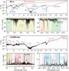Fig. 1

Spectra of B1-c (top row) and L1448-mm (third row) and the main spectral features detected among the JOYS data of these two sources (two panels per source below the full spectrum). In the top spectrum of B1-c, the SED continuum fit is shown in red and dominant ice and silicate absorption features are labeled in blue and brown, respectively. The two gray boxes mark the spectral range covered in the two insets in the second row. The baseline-subtracted absorption spectra of B1-c are presented in the second row, highlighting the CO and rovibrational H₂O features between 4.9–7.0 µm and the CO₂, ¹³CO₂, C₂H₂, and HCN features between 13.3–15.9 µm. The third row shows the spectrum of L1448-mm with dominant emission lines of H₂, [S I], and [Fe II] labeled in red. The bottom row shows the baseline-subtracted emission spectra from the two gray boxes, focusing on the rovibrational H₂O, SO₂, CH₄, and SiO features between 7.0–8.6 µm and the pure rotational lines of H₂O and OH between 18.5–21.5 µm.

2.3.3 Molecular spectroscopy

The spectroscopic information needed for fitting the emission and absorption of all targeted molecules was taken from the HITRAN database² (Gordon et al. 2022). The full list of molecules included in this work contains H₂ O, CO, OH, CO₂, ¹³CO₂, C₂H₂, ¹³CCH, HCN, C₄H₂, CH₄, SO₂, CS, SiO, and NH₃. The most relevant spectroscopic information is the rest wavelength, upper energy level, E_up, Einstein A_ij coefficients, and upper level degeneracy, 𝑔_up, for each transition. The HITRAN data were converted to the Leiden Atomic and Molecular Database (LAMDA; Schöier et al. 2005; van der Tak et al. 2020) format to make it compatible with the radexpy slab model code (e.g., Grant et al. 2023; Tabone et al. 2023; Francis et al. 2024). The partition functions, Q, as a function of temperature were similarly obtained from the HITRAN database. The partition function of SiO was taken from the Cologne Database for Molecular Spectroscopy³ (CDMS; Müller et al. 2001, 2005; Endres et al. 2016).

2.3.4 Local thermodynamic equilibrium model fitting

For each molecule, the best fitting excitation temperature, T_ex, and column density, N, were determined by setting a grid covering a large range of conditions (see e.g., Francis et al. 2024). Two different grids are explored in this work. One higher resolution grid covers T_ex = 50–800 K in steps of 10 K and log₁₀(N) = 14–21 in units of cm⁻² with steps of 0.125 on a log₁₀ scale. The second grid has a lower resolution but covers a larger range in both T_ex and N: 50–2500 K in steps of 25 K and log₁₀(N) = 14–23 in units of cm⁻² with steps of 0.167 on a log₁₀ scale. The higher resolution grid is applicable to most molecules since typical temperatures measured lie in the 100–500 K range. However, for CO, OH, and in some cases H₂O, higher temperatures (up to 2000 K) were measured, necessitating the need for exploring a broader parameter space.

Given that H₂O could not be fit by an LTE model with a single excitation temperature in many sources, multiple components were used that probe different reservoirs of H₂O in the protostellar system with different temperatures (see e.g., Gasman et al. 2023; Temmink et al. 2024a). Here, three different components are adopted. All the rovibrational lines shortward of 9 µm were fit using a single LTE model (Rovib H₂O). The pure rotational lines longward of 11 µm were fit using a colder (T ~ 100–300 K) and warm (T > 300 K) component.

Absorption and emission model grids were computed separately. For each grid point, the optical depth as a function of wavelength was computed on a high spectral resolution of R = 10⁶ taking into account line overlap producing optically thick lines (Tabone et al. 2023). For emission models, the intrinsic line broadening ∆V was set to the commonly adopted value of 4.71 km s⁻¹ based on the thermal line broadening of H₂ molecules at 500 K (Salyk et al. 2011). It is important to note that in case of optically thin emission, the derived column density is independent of ∆V, whereas for optically thick emission, the column density scales with ∆V⁻¹ (e.g., Tabone et al. 2023). For absorption models, on the other hand, the depth of absorption features is more dependent on the assumed ∆V. Since determining ∆V accurately for the sample is not the main goal of this paper, only a few values of ∆V (2, 4.71, 10, and 20 km s⁻¹) were explored in order to get good fits to the data. Larger ∆V were tested by visual inspection, but did not improve the fit for any of the sources.

The radial velocity offset (υ_line) with respect to the υ_lsr was determined for CO₂, SiO, and H₂O in our three most line-rich sources, B1-c, L1448-mm, and BHR71-IRS1, through Gaussian fitting of selected unblended lines. For H₂O, the rovibrational lines and rotational lines were fit separately. Since multiple lines of the same species were included, the uncertainty of the velocity could be derived at the level of ~5 km s⁻¹. The υ_line of all other species was determined by visual inspection with a typical uncertainty of ~ 10–20 km s⁻¹. The aim of this paper is not to derive accurate velocity information for all sources and species, but only for the selected sources and species for which more accurate velocities are needed in interpreting the results. For all other sources and species, υ_line will be derived in future works focusing on spatially extended molecular emission in the outflows.

For absorption models, the χ² was minimized for each grid point on the optical depth scale following the description of Francis et al. (2024) which is based on earlier work of Helmich (1996), $χ^{2} = \sum_{i = 1}^{N_{bin}} {(\frac{τ_{obs, i} - τ_{model, i}}{τ_{σ}})}^{2},$ ${\chi ^2} = \sum\limits_{i = 1}^{{N_{{\rm{bin}}}}} {{{\left( {{{{\tau _{{\rm{obs}},{\rm{i}}}} - {\tau _{{\rm{model }},{\rm{i}}}}} \over {{\tau _\sigma }}}} \right)}^2}} ,$ (3)

where N_bin is the number of selected wavelength bins used in the fit, τ_obs is the observed line optical depth defined as τ_obs = − ln(F_obs/F_baseline) with F_obs the observed flux (in mJy) and F_baseline the local continuum baseline (in mJy) determined in Sect. 2.3.1, τ_model is the model optical depth, and τ_σ the uncertainty on the optical depth defined as τ_σ = σ/F_obs with σ the noise level in mJy presented in Table C.1. In order to match the observations, the optical depth of the model in Eq. (3) (τ_model) was scaled to the MIRI-MRS resolution as a function of wavelength (R = 3500 − 1000; Labiano et al. 2021; Jones et al. 2023; Argyriou et al. 2023; Pontoppidan et al. 2024).

In the case of emission, the model optical depth as function of wavelength was first converted to the model flux (F_model) before calculating the χ² via $F_{model} = π {(\frac{R_{em}}{d})}^{2} B_{v} (T_{ex}) (1 - e^{τ_{model}}),$ ${F_{{\rm{model }}}} = \pi {\left( {{{{R_{{\rm{em}}}}} \over d}} \right)^2}{B_v}\left( {{T_{{\rm{ex}}}}} \right)\left( {1 - {e^{{\tau _{{\rm{model}}}}}}} \right),$ (4)

where d is the distance to the source, R_em is the radius of the emitting area, and B_ν(T_ex) is the Planck function at the excitation temperature of the corresponding grid point. In Eq. (4), the emitting area was parameterized as a circle with a radius, R_em, but in reality the emitting area can have any shape with an area equal to $π R_{em}^{2}$ $\pi R_{{\rm{em}}}^2$ . In contrast to absorption models, emission models thus have one additional parameter, R_em, related to the size of the emitting area which was needed to scale the model to the observed flux. In case of optically thin emission, N and R_em are completely degenerate with each other, but for optically thick emission, N and R_em can both be constrained. Using the model flux, the χ² for each grid point was calculated analogous to Eq. (3), $χ^{2} = \sum_{i = 1}^{N_{bin}} {(\frac{F_{obs, i} - F_{model, i}}{σ})}^{2},$ ${\chi ^2} = \sum\limits_{i = 1}^{{N_{{\rm{bin }}}}} {{{\left( {{{{F_{{\rm{obs }},i}} - {F_{{\rm{model}},{\rm{i}}}}} \over \sigma }} \right)}^2}} ,$ (5)

with σ the noise level (in mJy) for each band listed in Table C.1.

In contrast to absorption models, it is important to take into account the extinction to provide a good fit to the data and derive accurate column densities. This is especially important for species with transitions in deep ice absorption features (e.g., CO₂ P branch lines in the CO₂ ice feature; Francis et al. 2024; van Gelder et al. 2024). The extinction described in Sect. 2.3.2 was applied to the LTE model before computing the χ².

Only wavelengths that show emission or absorption features were included in the fit, while wavelengths overlapping with strong atomic or H₂ lines were excluded. Furthermore, the shape of the Q branch of molecular emission or absorption features is very sensitive to the excitation temperature but is also very degenerate with line optical depth. Hence, even though the line optical depth was taken into account in the LTE models, strongly blended lines such as Q branches were omitted in the fit to not suffer from high line optical depths. This indeed improves the accuracy of the derived excitation temperatures and column densities (see the discussion in Appendix E, available on Zenodo and also Li et al. 2024). However, Q branches or other possibly optically thick lines were included if these were the only detected lines (i.e., when both R and P branches were not detected). Following the procedure of Grant et al. (2023) and Francis et al. (2024), an iterative fit of the molecules was performed in order of decreasing flux where the best-fit model for each molecule was subtracted before continuing to the next molecule.

The best-fit model was determined by the minimum χ² of the grid. The confidence intervals of T_ex, N, and R_em (for emission models) were determined following Carr & Najita (2008) and Salyk et al. (2011) by placing contours on the χ² maps. Similarly, the best-fit number of molecules 𝒩_mol of emission models was computed via $N_{mol} = N π R^{2},$ ${{\cal N}_{{\rm{mol}}}} = N\pi {R^2},$ (6)

and its confidence intervals were calculated similarly to those of T_ex and N. The number of free parameters K was set to 2 (see discussion in Avni 1976), and the 1, 2, 3σ confidence intervals were computed from the reduced χ² $(χ_{red}^{2} = χ^{2} / K)$ $\left( {\chi _{{\rm{red}}}^2 = {\chi ^2}/K} \right)$ by setting a $Δ χ_{red}^{2}$ $\Delta \chi _{{\rm{red}}}^2$ of 2.3, 6.2, and 11.8, respectively.

A molecule (or component of H₂O) was considered detected when at least three wavelength bins showed emission or absorption above the 5σ level. For the cases in which no accurate constraints on the parameters could be achieved for a certain molecule (e.g., ¹³CO₂ and ¹³CCH₂ in L1448-mm), the temperature was fixed to that of other species in the same source and only the column density and emitting area were fit for. Moreover, in case of non-detections, the 3σ upper limit to the column density was derived for a typical excitation temperature of 150 K and setting the emitting radius to a typical radius of 10 au. It is important to note that the emission (and absorption) was assumed to be optically thin and the resulting upper limit on 𝒩_mol is therefore not dependent on the assumed radius. For the warm H₂O component, an excitation temperature of 450 K was set when deriving the 3σ upper limit to the column density.

2.3.5 Infrared pumping

Column densities derived from absorption lines are not susceptible to possible non-LTE effects such as infrared pumping. However, for column densities (or number of molecules) derived from emission line models, this has to be taken into account so that these parameters are not overestimated (e.g., Boonman et al. 2003; Bruderer et al. 2015; Bosman et al. 2017; van Gelder et al. 2024). The most direct way to take infrared pumping into account would be to run a grid of non-LTE RADEX models (van der Tak et al. 2007; Bruderer et al. 2015; Bosman et al. 2017), but this is beyond the scope of this work and only possible for a select number of molecules (i.e., H₂O, CO₂, and HCN) for which collisional rate coefficients are available. It would also require detailed physical and chemical model of the source with the infrared radiation field specified at each point. An indirect method is through measurements of the same molecules at sub-millimeter wavelengths in their pure rotation transitions as was done for SO₂ in NGC 1333 IRAS 2A (van Gelder et al. 2024), but this is not possible for molecules such as CH₄, CO₂, and C₂H₂ that lack pure rotational transitions at millimeter wavelengths due to the absence of a permanent dipole moment.

Nevertheless, the effect of infrared pumping can be estimated when assuming the vibrational temperature (T_vib) is set by the infrared radiation field (as was the case for SO₂ in NGC 1333 IRAS 2A; van Gelder et al. 2024). The vibrational temperature is then approximately equal to the brightness temperature (T_IR) at the frequency (v) of the vibrational mode through which the IR pumping occurs, $T_{vib} \approx T_{IR} = \frac{h v}{k_{B}} \ln^{- 1} (1 + \frac{2 h v^{3}}{I_{v} c^{2}}),$ ${T_{{\rm{vib}}}} \approx {T_{{\rm{IR}}}} = {{hv} \over {{k_{\rm{B}}}}}{\ln ^{ - 1}}\left( {1 + {{2h{v^3}} \over {{I_v}{c^2}}}} \right),$ (7)

where I_v is the extinction corrected surface brightness (in Jy sr⁻¹), h is Planck’s constant, k_B is the Boltzmann constant, and c is the speed of light. The corrected number of molecules (𝒩_mol,corr) can then be computed via (van Gelder et al. 2024) $N_{mol, corr} = N_{mol} \frac{e^{- h v / (k_{B} T_{rot})}}{e^{- h v / (k_{B} T_{vib})}},$ ${{\cal N}_{{\rm{mol}},{\rm{ corr }}}} = {{\cal N}_{{\rm{mol}}}}{{{e^{ - hv/\left( {{k_{\rm{B}}}{T_{{\rm{rot}}}}} \right)}}} \over {{e^{ - hv/\left( {{k_{\rm{B}}}{T_{{\rm{vib}}}}} \right)}}}},$ (8)

where 𝒩_mol is the number of molecules measured from the LTE model fits (Sect. 2.3.4) and T_rot is the rotational temperature in the vibrational ground state (assumed to be equal to T_ex measured from the LTE model fits; van Gelder et al. 2024). Statistical degeneracies, 𝑔, have been neglected in Eq. (8) for simplicity but this does not significantly affect the derived 𝒩_mol,corr since the uncertainties on T_ex and T_vib dominate the uncertainty of 𝒩_mol,corr (see discussion below). The correction was only applied to species that are detected and not to derived upper limits on 𝒩_mol.

It is important to take into account that the IR pumping does not necessarily go through the vibrational level of the observed emission. For CO₂, for example, pumping can occur through the V₃ mode around 4.3 µm followed by de-excitation through other vibrational bands such as the v₂ bending mode around 15 µm (Bosman et al. 2017). Many of the detected molecules have vibrational modes at shorter wavelengths (i.e., higher T_IR) than those that are detected here (e.g., C₂H₂ with the v₄ + v₅ mode around 7.7 µm, which is not detected in our data). The bands through which the IR pumping is assumed to occur are presented in Table 1. For CO₂, the brightness temperature at 4.3 µm (i.e., outside the MIRI-MRS range) was obtained from a NIRSpec program (PID: 1960) within the JOYS collaboration (private communication) or through interpolation of the SED to shorter wavelengths for sources where NIRSpec data is not available.

Computing 𝒩_corr comes with some significant uncertainties (i.e., T_vib ≈ T_IR, pumping through higher order excited states, neglecting ɡ factors; see the discussion in Appendix D, available on Zenodo). Small differences of 5–10 K in the derived T_vib can already lead to an order of magnitude difference in the derived 𝒩_corr (see Fig. D.1). The uncertainty on 𝒩_corr can therefore be orders of magnitude even when the difference between T_vib and T_rot is small. Nevertheless, it is important to provide an estimate for the effect of infrared pumping on the derived number of molecules. Therefore, only the minimum and maximum values of 𝒩_corr are presented, where the maximum value of 𝒩_corr corresponds to the uncorrected 𝒩_mol and the minimum value of 𝒩_corr to that computed using Eq. (8). A full non-LTE analysis, taking all these effects into account, is beyond the scope of this work.

Table 1

Infrared pumping information for each molecule.

2.3.6 Abundances

Column densities or total number of molecules by themselves do not provide accurate constraints on the abundance of a molecule due to observational dependencies (i.e., emitting area). The ratio between two molecules, on the other hand, do provide such constraints, assuming that the two molecules are roughly located in the same region of the protostellar system. It is, however, important that a relevant reference species is selected.

In this paper, all abundance ratios were taken with respect to H₂O since it is a dominant ice species and because it is abundantly detected in many sources. Water is therefore an excellent reference species for ice sublimation in hot cores. High-temperature gas-phase chemistry in either the hot core or in shocks can also produce H₂O, but as long as the H₂O is just recycled in the hot gas (i.e., destroyed and reformed), it is still a good reference species. The main issue would be if there is a significant amount oxygen not originally in H₂O ice or gas (e.g., atomic O, refractory dust) that is driven into H₂O by high-temperature gas-phase chemistry, but this cannot contribute to the amount of H₂O by more than a factor of a few (see e.g., van Dishoeck et al. 2021).

Water shows emission or absorption lines through both its rovibrational lines between 5–9 µm and its pure rotational lines longward of 13 µm. However, the ro-vibrational lines are susceptible to IR pumping effects (see Sect. 2.3.5) whereas the pure rotational lines are not. On the other hand, the pure rotational lines at mid-IR wavelengths originate from high energy levels of several thousands of K, needing warm gas to be excited, whereas rovibrational lines in absorption originate from the ground state with E_low as low as 0 K, therefore being more sensitive to the cold gas. Nevertheless, given that the derived temperatures of H₂O from the pure rotational lines are low (100–500 K) and in order to avoid the effect of infrared pumping, the total column density (absorption) or number of molecules (emission) of H₂O was derived from the pure rotational lines. The rotational lines were fit using two components (cold, warm) and the total column density or number of molecules was calculated through the sum of these two components. In the majority of the sources, the total rotational H₂O component (hereafter H₂O-rot) is dominated by the cold component, although for some sources this is not detected (e.g., B1-c).

An alternative to H₂O as a reference species would be CO₂, which is also a dominant ice species detected toward many of the sources with a rather constant CO₂/H₂O ice ratio (e.g., Pontoppidan et al. 2008). However, gaseous CO₂ appears to be more often associated with disk winds or outflowing material and its derived column density or number of molecules is often uncertain due to IR pumping. Molecular hydrogen is another option as it is the most abundant molecule and would provide absolute abundances. However, the emission of the low-J lines, which are most sensitive to the warm (~few 100 K) gas, is dominated by the outflow or disk winds (e.g., Tychoniec et al. 2024, Francis et al., in prep.), making it difficult to disentangle the contribution from the warm inner envelope and disk. Therefore, H₂O was selected as the reference species for abundance ratios.

3 Results

3.1 Continuum emission

Within the JOYS low-mass sample, 18 continuum point sources are detected (see Appendix B). The binary B1-a is only very marginally resolved at the shortest wavelengths (see Fig. B.1) and fully unresolved from ~12 µm onward, and therefore analyzed as a single source B1-a-NS. On the other hand, the TMC1 binary is resolved up to ~16 µm (see Figs. B.15 and B.16) and therefore both components are analyzed individually. At longer wavelengths, the binary becomes unresolved, which could explain the similar temperature of the cold H₂O components (see Appendix A.1). However, this does not affect any of the derived conclusions. For L1527, the continuum traces the scattered light on both sides of the disk (see Fig. B.13).

Neither IRAS 4B nor Ser-S68N-S is detected at its source position (based on ALMA data; Tychoniec et al. 2021) in the continuum over the full MIRI-MRS wavelength range. For Ser-S68N-S, some continuum flux appears to be present longward of 12 µm, but this likely originates from the wings of the PSF from Ser-S68N-N (see Fig. B.8). Both IRAS 4B and Ser-S68N-S are likely too embedded to be detectable even at MIRI-MRS wavelengths, similar to the case of HH 211 (Ray et al. 2023; Caratti o Garatti et al. 2024). Ser-S68N-S has an outflow oriented nearly in the plane of the sky (i.e., edge-on disk; Podio et al. 2021), which could also explain the lack of continuum emission, but for IRAS 4B the orientation of the outflow is unknown (Podio et al. 2021). Toward the source position of IRAS 4B no clear molecular features are present, but in particular strong emission of H₂O is detected in the jet about 4″ to the south for IRAS 4B, as was also seen by Herschel (Herczeg et al. 2012), which will be discussed in a separate paper. Toward Ser-S68N-S, weak CO and CO₂ emission is detected around 5 µm and 15 µm, respectively, which is likely related to the strong molecular outflow (Tychoniec et al. 2019, Francis et al. in prep.). Additionally, H₂O and OH emission is detected at >20 µm wavelengths, but this is likely related to Ser-S68N-N, since its PSF starts overlapping with that of Ser-S68N-S at longer wavelengths. IRAS 4B and Ser-S68N-S are therefore excluded in the remainder of the analysis. However, it is important to note that the absence of molecular features in the spectra in these two sources does not mean that the molecules are absent in these systems but are possibly hidden due to the high extinction by their natal envelopes and/or dusty accretion disks.

3.2 Molecular spectra

An overview of the two most line-rich spectra of the JOYS sample, B1-c and L1448-mm, is presented in Fig. 1. For B1-c, the baseline-subtracted spectrum around a few key wavelength ranges is also presented in Fig. 2. The spectra show an unprecedented richness in gas-phase molecular features across the full wavelength range, as well as multiple deep ice absorption features. These ice features include both simple (i.e., H₂O, CO₂, CH₄, NH₃) and complex (e.g., CH₃OH, C₂H₅OH, CH₃OCHO) molecules and are presented in separate papers (e.g., Rocha et al. 2024; Chen et al. 2024; Brunken et al. 2024; Slavicinska et al. 2024). Multiple sources also show emission of H₂ (not analyzed in this work) and atoms (i.e., [S I], [Fe II]) tracing mostly the disk wind, outflow, or jet (e.g., Tychoniec et al. 2024). The molecular gas-phase lines are detected both in absorption (e.g., B1-c, BHR71 IRS1) and in emission (e.g., B1-a-NS, L1448-mm) toward the JOYS sources.

The shorter wavelengths (i.e., <7 µm) are dominated by features from the first overtone of CO and the ν₂ rovibrational lines of H₂O (see for TMC1-W in Fig. 3). Only the J > 25 P branch lines of CO are covered in the MIRI-MRS wavelength range. The rovibrational lines of H₂O are commonly detected toward the JOYS sources (see Sect. 3.3), both in emission and in absorption. In several sources (e.g., B1-c, TMC1-W; see Figs. 2 and 3), the forest of H₂O lines is so dense that almost no line-free wavelength regions are present.

At longer wavelengths (i.e., >7 µm), other molecular features start to appear, such as those of the SO₂ ν₃ band with the Q branch at 7.35 µm (see also van Gelder et al. 2024) and the CH₄ ν₄ mode with its Q branch at 7.65 µm. Interestingly, clear emission (L1448-mm) and absorption (BHR71-IRS1) features of SiO are detected between 8-8.5 µm (see Fig. 4). This triples the number of SiO detections at mid-IR wavelengths toward protostellar systems (see e.g., McClure et al. 2024). Moreover, toward B1-c, clear absorption features associated with CS and NH₃ are detected (see Fig. 5), marking the first detection of these molecules at mid-IR wavelengths toward a low-mass protostellar system.

In channel 3B (i.e., 13 < λ < 15.5 µm), the bands of C₂H₂ (ν₅, Q branch at 13.6 µm), HCN (v₂, Q branch at 14.1 µm), and CO₂ (v₂, Q branch at 15.0 µm) are located (see the case of B1-c in Fig. 2). Next to the Q branch of C₂H₂, also its ¹³CCH₂ iso-topolog is detected toward both B1-c and L1448-mm. Similarly, the Q branch of ¹³CO₂ at 15.45 µm is detected toward both of these sources (see Figs. 1 and 2). Toward L1448-mm, also di-acetelyne (C₄H₂) is observed in emission through its ν₈ bending mode at 15.92 µm.

The longest wavelengths (i.e., >17 µm) are dominated by OH features and the pure rotational transitions of H₂O (see bottom right panel of Fig. 1). The rotational lines of H₂O originate from energy levels of >1000 K and are therefore mostly sensitive to warmer temperatures. However, some rotational transitions are clearly sensitive to colder temperatures of ~ 100-200 K than the bulk of the lines which trace T > 300 K gas.

All together, the JOYS data provide a wealth of molecular emission and absorption features of various molecules. In Sects. 3.3 and 3.4, the detection statistics and LTE slab model fit results will be presented. The LTE models provide remarkably good fits to the data (see e.g., Fig. 2 for B1-c). In Appendix F (available on Zenodo), the residuals of the full LTE fit to B1-c are presented. The residuals show remaining absorption lines which could either originate from either a different temperature component to the fit molecular species or a species that is not considered in this paper (e.g., isotopologs). Nevertheless, the residuals are mostly below the level of 10% with higher residuals in some line-rich wavelength regions (e.g., 7–8 µm; see Fig. F.2).

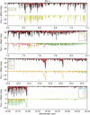Fig. 2

Overview of the main molecular absorption features detected toward B1-c in the MIRI-MRS wavelength range. In each panel, the baseline-subtracted spectrum is shown in black and the best-fit LTE model including all molecules listed is overlaid as the shaded red area. At the bottom of each panel, the individual best-fit LTE models of all molecules contributing to the corresponding wavelength range are displayed at an arbitrary constant offset, with each color denoting a different species. The surprising detection of NH₃ toward B1-c is highlighted in Fig. 5.

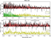Fig. 3

Baseline-subtracted spectrum (black) and best-fit LTE model (shaded red) for TMC1-W in the 4.9–8.0 µm range. At the bottom of each panel, the individual best-fit LTE models of rovibrational H₂O (yellow) and CO (green) are shown at an arbitrary constant offset. Deep negative absorption features originating from detector artifacts are clipped for clarity.

3.3 Molecular detection statistics

The molecular detections per source are listed in Table H.1 (available on Zenodo). The most commonly observed molecule is H₂O, which is detected toward 12/16 of the studied sources. The rovibrational lines around 5-8 µm are detected in three more sources (11/16) than the pure rotational lines longward of 13 µm (8/16). This could be related to the decrease in sensitivity at longer wavelengths (see Table C.1). However, it is just opposite to what is observed toward more evolved Class II disks where the pure rotational lines appear to be more often detected than the rovibrational lines, likely due to subthermal excitation of the vibrational levels (see e.g., Banzatti et al. 2023b). Moreover, three of the four sources with rovibrational H₂O detected but an absence of rotational H₂O (Ser-SMM1B, TMC1A, BHR71-IRS2) show the rovibrational lines in absorption. These absorption lines originate from the vibrational ground state with E_low as low as 0 K, whereas the pure rotational lines originate from much higher energy levels (>1000 K), which could explain their absence. The other source, L1527, shows only a few rovibrational lines of H₂O weakly in emission and only located in the western side of the disk or outflow (Devaraj et al., in prep.), which could mean that they are the result of IR pumping rather than colli-sional excitation. B1-c is the only source that shows absorption of H₂O in the pure rotational lines arising from E_low > 1000 K levels. Interestingly, the pure rotational lines of H₂O are in emission toward BHR71-IRS1 whereas the rovibrational lines are in absorption, indicating that they are likely tracing two different components (e.g., hot core, disk wind or outflow) within the protostellar system. Moreover, the rovibrational lines are seen in absorption toward TMC1-E whereas they are in emission toward TMC1-W.

Almost as commonly detected as H₂O is CO₂, which is seen toward 11/16 sources. Similar to H₂O, it is mostly observed in emission, but is in absorption toward four sources. In the case of Ser-S68N-S, the CO₂ emission is clearly spatially offset and located in the outflow rather than at the central position and is therefore excluded from the remaining analysis. Toward several other sources (e.g., L1448-mm, BHR71-IRS1, Ser-SMM3), CO₂ also shows an outflow component but hosts a bright central component as well. The ¹³CO₂ isotopolog is only detected toward the two sources that are most rich in molecular features, B1-c (in absorption) and L1448-mm (in emission).

Other molecules are far less present than H₂O and CO₂. Besides CO and OH, which are discussed further below, C₂H₂ and CH₄ are the most detected species (3/16). Several other species such as ¹³CCH₂, HCN, and SO₂ are only detected toward B1-c and L1448-mm. The carbon-chain molecule C₄H₂, commonly observed in more evolved Class II disks around very low-mass stars (e.g., Tabone et al. 2023; Arabhavi et al. 2024), is detected in emission only toward L1448-mm. Silicon monoxide is detected in emission (L1448-mm) and absorption (BHR71-IRS1) around 8.5 µm (see Appendix A.9). Toward B1-c, also CS (8–8.5 µm) and NH₃ (9–11 µm) are detected in absorption for the first time toward a low-mass protostellar system.

Lastly, CO and OH are commonly detected toward the JOYS sources (8/16 and 7/16, respectively). Carbon monoxide is seen in absorption toward the sources that also show the rovibra-tional H₂O lines in absorption except for TMC1-E, where CO is in absorption but the rovibrational lines of H₂O are in emission. However, only the high-J lines of the P branch of CO are detectable with MIRI-MRS; hence, a non-detection of CO here does not imply that it is not present in the protostellar systems. Furthermore, because only the high-J lines are detectable, the LTE analysis is degenerate between high temperatures and high column densities (e.g., Herczeg et al. 2011; Francis et al. 2024, see also discussion in Rubinstein et al. 2024 for the NIRSpec range) and will therefore not be further discussed in this paper. The OH radical is only detected in emission. Toward several sources (e.g., B1-a-NS, TMC1-E, BHR71-IRS1), prompt OH emission is detected between 9-11 µm, which is suggested to originate from H₂O photodissociation (Tabone et al. 2021, 2024; Zannese et al. 2024; Neufeld et al. 2024). In all sources with OH detections, also the lines at longer wavelengths (>13 µm) are detected which likely result from formation pumping (e.g., Carr & Najita 2014; Zannese et al. 2024). Since the OH emission is therefore likely not originating from regions that are in LTE, it will also not be discussed further in this paper.

The JOYS data were also checked for other molecules including H₂S and hydrocarbons such as C₆H₆, C₂H₄, C₂H₆, and CH₃ that are often detected toward Class II disks around very low-mass stars (Tabone et al. 2023; Arabhavi et al. 2024). However, these molecules are not detected in any of the sources. Likewise, complex organics such as CH₃OH and CH₃CN have infrared bands in the MIRI-MRS wavelength range and are not detected toward any of the sources. Furthermore, the MIRI-MRS spectral range also covers cations such as N₂H⁺, HCO⁺, and ${CH}_{3}^{+}$ ${\rm{CH}}_3^ +$ , but these are also not detected toward any of the sources.

Three sources (i.e., B1-b, Per-emb 8, Ser-SMM1A) do not show any gas-phase molecular features in their spectra albeit a clear detection of the continuum across the full wavelength range (see Figs. B.2, B.6, and B.9). Here, the absence of molecular features cannot be explained by envelope or cloud extinction as is likely the case for IRAS 4B and Ser-S68N-S.

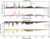Fig. 4

Baseline-subtracted spectrum (black) and best-fit LTE model (shaded red) for L1448-mm (top panel) and BHR71-IRS1 (bottom panel) in the 7.2–8.6 µm range. At the bottom of each panel, the individual best-fit LTE models of rovibrational H₂O (yellow), CH₄ (red), SO₂ (pink), and SiO (brown) are shown at an arbitrary constant offset. Deep negative absorption features originating from detector artifacts are clipped for clarity.

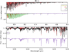Fig. 5

Baseline-subtracted spectrum (black) and best-fit LTE model (shaded red) for B1-c in the 8.2-12.5 µm range. At the bottom of each panel, the individual best-fit LTE models of rovibrational H₂O (yellow), CH₄ (red), CS (green), and NH₃ (purple) are shown at an arbitrary constant offset. Deep negative absorption features originating from detector artifacts are clipped for clarity. Between 10-12 µm, some features of NH₃ are over or under reproduced, but the S/N at these wavelengths is low due to the strong absorption by the silicate and H₂O ice libration bands.

3.4 Local thermodynamic equilibrium model fit results

As an example of our results, an overview of the main molecular features detected toward B1-c and the best-fit LTE model is shown in Fig. 2. The full baseline-subtracted spectra are presented in Appendix G (available on Zenodo) for all sources.

The overlaid best-fit model clearly presents a very good fit to the data, with the majority of the absorption features fit by the molecules listed in Fig. 2. It is important to note that the 9–12 µm range of the continuum subtracted spectra presented in Appendix G is more noisy due to the deep silicate and water libration mode absorption. Moreover, the discrepancy between the R and P branches due to the extinction of the CO₂ ice band is evident: almost no absorption features are present between 15 µm and 15.4 µm, which is nicely consistent with the LTE models (i.e., there is no continuum to absorb against). Similarly, for L1448-mm this effect is very evident for CO₂ in emission, as it was to a lesser extent also for the P and R branch lines in the high-mass source IRAS 23385+6053 (Francis et al. 2024).

The main findings per molecule are presented in Appendix A. In Table 2, the derived excitation temperatures are presented for all sources showing molecular emission or absorption features. The best-fit LTE results (i.e., column density N, excitation temperature T_ex, radius of emitting area R_em, number of molecules 𝒩_mol, number of molecules corrected for infrared pumping 𝒩_mol,corr) are tabulated per source in Appendix H (available on Zenodo).

It is important to note that the results from absorption modeling (i.e., B1-c, BHR71-IRS1) are very reliable since they are not dependent on an emitting area and do not suffer from non-LTE effects such as IR pumping. The results from emission models (i.e., L1448-mm) are therefore more uncertain. Nevertheless, the majority of the excitation conditions (T_ex) are well constrained (typical error of ~10 K) and are rather cold in the range of T_ex ~ 100–300 K for most species. Similarly to T_ex, column densities (N) and number of molecules (𝒩_mol) are within a few orders of magnitude for the majority of the sources.

Table 2

Excitation temperatures in units of Kelvin derived from the LTE slab models.

4 Discussion

4.1 Hot core versus outflow

One key question is what the molecular emission and absorption features in the JOYS data are tracing. Most molecules have temperatures in the range of 100–300 K, which means that they are likely associated with the hot core and warm inner envelope or alternatively with dense shocks in the outflow. A direct way to distinguish between ice desorption in the hot core or gas-phase chemistry is by comparing the abundance ratios with respect to H₂O between ice and gas. Assuming that the amount of H₂O is dominated by thermal ice desorption, similar abundances between gas and ice point toward an origin of the molecules in the ices whereas deviating abundances hint at (subsequent) gas-phase chemistry. However, H₂O can also have gas-phase formation routes in the hot core, but as long as H₂O is only recycled (i.e., destroyed and reformed) in the gas phase, the amount of H₂O will not be altered significantly. Only if large amounts of oxygen are driven from another form (e.g., atomic, refractory dust) into H₂O, its abundance (with respect to H₂) will be increased, but not by more than a factor of a few (see e.g., van Dishoeck et al. 2021). Outflowing material is most directly recognized by a blueshifted velocity offset, such as for BHR71-IRS1 (v_line up to −45 km s⁻¹), or spatially extended emission such as for L1448-mm and B1-a.

Only H₂O and CO₂ are detected toward a larger bulk of sources. The majority of the species are predominantly detected toward B1-c and L1448-mm, with some other detections toward other sources such as BHR71-IRS1 (C₂H₂, SiO). The discussion below on what the mid-IR molecular features are tracing is therefore biased toward B1-c and L1448-mm, but also information from (non)detections in the other sources is included.

4.1.1 Hot cores

The strongest indication for the mid-IR gas-phase lines tracing ice sublimation in a hot core is the case of B1-c. Both the gas-phase and ice abundance ratios with respect to H₂O are shown in Fig. 6. B1-c is one of the prototypical hot core sources that is rich in complex organics at millimeter wavelengths with no evidence of an embedded disk down to 10 au scales (van Gelder et al. 2020; Nazari et al. 2021). Moreover, it is also a bright infrared source showing many deep ice absorption features (e.g., Fig. 1; Boogert et al. 2008; Pontoppidan et al. 2008; Öberg et al. 2008; Chen et al. 2024). It is directly evident that the abundances between gas and ice are remarkably similar. It is important to note that the gas-phase column densities and their ratios for B1-c are derived from absorption lines and therefore more reliable than those derived for sources showing emission lines. Moreover, the velocity of all absorbing species is consistent with the υ_lsr = 6 km s⁻¹, therefore excluding an outflow origin since its outflow is not in the plane of the sky (e.g., Jørgensen et al. 2006; Hatchell et al. 2007; Tychoniec et al. 2021). In particular the ratios of CO₂ (i.e., the ¹³CO₂ ratio multiplied by 70) and NH₃ are in very good agreement with these in the ices, showing that the gas-phase lines are directly tracing the composition of the sublimated ices. For CH₄, the gas-phase abundance is on the higher side but still within the uncertainties of typical CH₄ ice abundances (Öberg et al. 2008; Boogert et al. 2015; Rocha et al. 2024; Chen et al. 2024). The only species that significantly deviates is SO₂ for which the gas-phase abundance is about an order of magnitude higher than in the ices (Rocha et al. 2024; Chen et al. 2024). This indicates that for SO₂ (additional) gas-phase chemistry may enhance its abundance above that of the ices (e.g., Charnley 1997; Garrod et al. 2022).

Similarly, for some other sources a hot core origin seems to be the most plausible. In Ser-SMM1B, CO₂ is detected in emission and the upper limits for other species such as SO₂, and NH₃ are all still consistent with ices. An ice origin is further supported by the velocity of the CO₂ that is redshifted by ~10 km s⁻¹ with respect to the υ_lsr, likely coming from infalling material. However, only the Q branch of CO₂ is detected and therefore the number of CO₂ molecules may be underestimated. SVS4-5 is another source showing deep ice absorption features (Pontoppidan et al. 2004; Perotti et al. 2020). The gas-phase ratios of CO₂ and CH₄ with respect to H₂O also point toward a hot core origin, but the lines are shifted by −80 km s⁻¹ and −40 km s⁻¹ with respect to the υ_lsr and are more consistent with outflowing material (i.e., molecules in the spatially extended outflow of the nearby Class 0 source Ser-SMM4 seen in absorption against the IR continuum of SVS4-5; Pontoppidan et al. 2004).

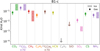Fig. 6

Abundance ratios of several detected molecules (colored datapoints) with respect to the total column density of H₂O derived from the pure rotational lines (cold + warm components) toward B1-c. The datapoints of ¹³CO₂ and ¹³CCH₂ are multiplied by 70 to take into account the ¹²C/¹³C ratio of the local ISM (Milam et al. 2005). The range of column density ratios detected in the ices for all low-mass protostellar systems (i.e., not limited to B1-c or other JOYS sources) are displayed as the shaded colored area for each species with a confirmed ice detection (Boogert et al. 2015; Rocha et al. 2024; Chen et al. 2024).

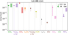Fig. 7

Abundance ratios in of several detected molecules (colored datapoints) with respect to the total number of molecules of H₂O derived from the pure rotational lines (cold + warm components) toward L1448-mm. The datapoints of ¹³CO₂ and ¹³CCH₂ are multiplied by 70 to take into account the ¹²C/¹³C ratio of the local ISM (Milam et al. 2005). The larger lighter error bars indicate the range of the abundance ratios when IR pumping is taken into account. The range of column density ratios detected in the ices for all low-mass protostellar systems (i.e., not limited to L1448-mm or other JOYS sources) are displayed as the shaded colored area for each species with a confirmed ice detection (Boogert et al. 2015; Rocha et al. 2024; Chen et al. 2024).

4.1.2 Outflows and disk winds

A completely different case to the hot core in B1-c is present in L1448-mm (see Fig. 7). Here, no strong agreement with the ices is seen for many species. Whereas the ratio of CO₂ is in agreement when IR pumping is not considered, its abundance with respect to H₂O may be as low as 10⁻⁵ when IR pumping through its 4 µm band is taken into account. Similarly, the upper limit for NH₃ suggests a lower gas-phase abundance than in the ices. On the other hand, the abundances of CH₄ and SO₂ are significantly higher than the ices. Given that the derived excitation temperatures of CH₄ and SO₂ (130 ± 10 K and 140 ± 20 K, respectively) are higher than the assumed vibrational temperatures (119 K and 122 K), their excitation is assumed not to be dominated by IR pumping, hence the latter cannot explain the high abundances of both species. Likewise to L1448-mm, the abundance ratios in BHR71-IRS1 do not agree with those in the ices.

This suggests that the molecular features are not directly tracing thermal ice sublimation but rather regions where their abundances are dominated by other effects. One possibility is that the molecular abundances are altered by gas-phase chemistry following thermal ice sublimation in a hot core (e.g., Charnley et al. 1992; Charnley 1997; Garrod et al. 2022). Alternatively, the molecular features could originate from shocks in either the outflow or disk wind close to the source, where they can be formed through high-temperature gas-phase chemistry (e.g., Caselli et al. 1997; Gusdorf et al. 2008a,b). Otherwise, the ices can be sputtered off the dust grains in such shocks, although this seems to be limited only to shock velocities of up to ≾15 km s⁻¹ (e.g., Suutarinen et al. 2014; van Dishoeck et al. 2021).

An (unresolved) outflow or disk wind origin is supported by the fact that the mid-IR lines are shifted by −10 up to −45 km s⁻¹ with respect to the υ_lsr in BHR71-IRS1. Toward L1448-mm, the velocity shift is smaller (~−25 km s⁻¹) and only directly evident at shorter wavelengths for the rovibrational lines of H₂O and SiO (see Table H.5). The emission lines of other molecules such as CO₂, C₂H₂, and HCN do not show significant velocity offsets up to −20 km s⁻¹. Moreover, especially CO₂ clearly shows spatially extended emission consistent with outflowing material (Navarro et al. in prep.). Furthermore, SiO is detected at mid-IR wavelengths toward both sources. Silicon monoxide is commonly observed at millimeter wavelengths in the bullets of molecular jets (e.g., Podio et al. 2016, 2021; Lee et al. 2017; Tychoniec et al. 2019, 2021) and indeed also detected on larger scales in the jets of both L1448-mm (Guilloteau et al. 1992; Jiménez-Serra et al. 2011; Toledano-Juárez et al. 2023; Nazari et al. 2024b) and BHR71-IRS1 (and IRS2; Gusdorf et al. 2011, 2015; Gavino et al. 2024). In both cases, the mid-IR SiO emission and absorption is spatially unresolved, but showing similar velocity offsets as the other molecules and atomic species (Tychoniec et al. in prep., Navarro et al., in prep.). This is in agreement with results from Herschel comparing the H₂O velocity profiles with those of SiO (e.g., Nisini et al. 2013; Leurini et al. 2014; van Dishoeck et al. 2021). Moreover, the derived temperatures of 300–400 K are consistent with those in jet shocks (e.g., Caselli et al. 1997; Gusdorf et al. 2008a,b) and not with thermal sublimation of silicate grains (~1500 K). Toward both sources, emission from other molecules such as CO₂ is also present in the MIRI-MRS data on larger scales in the outflows, but this will be presented in a separate paper.

For many other sources, there is also a strong indication that especially molecular emission features are tracing unresolved outflows. This is especially evident for CO₂, for which temperatures of ~100–300 K are measured for the majority of the sources, consistent with it being present on larger scales and not in the hot inner regions of an embedded disk (see Sect. 4.2). On the other hand, not all sources show velocity offsets in their CO₂ with respect to the υ_lsr (i.e., Ser-SMM3, TMC1A). Toward SVS4-5, the CO₂ emission is modeled at a velocity of −80 km s⁻¹ with respect to the υ_lsr, likely associated with the outflow of the nearby Class 0 source Ser-SMM4. For B1-a-NS, on the other hand, CO₂ is seen in absorption at +35 km s⁻¹ with respect to the υ_lsr, but also weak spatially extended emission of CO₂ is present toward the south. Overall, CO₂ appears to be very commonly present on larger scales and not necessarily solely tracing ice sublimation.

4.2 Embedded disks

4.2.1 Temperatures from Class 0 and I to Class II

Figure 8 compares the ranges of derived excitation temperatures from Class 0 and I sources in JOYS to those derived for more evolved Class II protoplanetary disks. Typical temperatures in Class II disks are T ≿ 500 K (e.g., Grant et al. 2023; Banzatti et al. 2023a; Gasman et al. 2023; Temmink et al. 2024a,b), suggesting that the emission arises either from the inner disk or a warm disk surface layer. In contrast, for many molecules, the derived temperatures (100–300 K) are significantly lower toward the protostars in the JOYS sample. As is discussed in Sect. 4.1, in many cases it is evident that the molecular features are not tracing a disk-like structure but are rather present in the hot core or warm inner envelope (e.g., B1-c, Ser-SMM1B) or are located in the disk wind or outflow (e.g., L1448-mm, BHR71-IRS1). However, in a few embedded sources, the rovibrational lines of H₂O show temperatures of up to 1200 K, suggesting that these may be tracing embedded disks.

Within the JOYS sample, several sources are known to host rotationally supported embedded disks based on resolved millimeter observations (e.g., TMC1A, TMC1, L1527; Tobin et al. 2012; Harsono et al. 2014; Tychoniec et al. 2021; Ohashi et al. 2023). Most notably, toward TMC1-W, hot H₂O (1280 ± 20 K) is detected through its rovibrational lines between 5.5 µm and 7.5 µm (see Fig. 3). Given the high temperature and the small emitting area predicted by the LTE models (0.05 ± 0.01 au), the rovibrational H₂O lines are clearly originating from hot compact material that likely resides within its inner embedded disk. Interestingly, toward its companion TMC1-E, the H₂O lines are in absorption and not as hot (580 ± 20 K), but still consistent with a cooler H₂O component in the disk (Gasman et al. 2023; Temmink et al. 2024a). Moreover, given that the lines are shifted by −10 km s⁻¹ with respect to the υ_lsr, this H₂O may also originate from a disk wind rather than the embedded disk (Tychoniec et al. 2024). Similarly hot H₂O as in TMC1-W is detected toward Ser-SMM1B (980 ± 20 K), but for this source the presence of an embedded disks has yet to be confirmed at millimeter wavelengths. However, given the similar temperature as seen toward TMC1-W, an embedded disk origin for the hot H₂O is plausible. Toward SVS4-5, also hot H₂O (1040 ± 20 K) is detected, which in contrast to CO₂ and CH₄ is not blueshifted but consistent with the systemic velocity. This indicates that it is likely originating from the background Class I/II source that is located behind or inside the envelope and outflow of the nearby Class 0 source Ser-SMM4 (Pontoppidan et al. 2004).

On the other hand, several sources hosting embedded disks do not show such hot temperatures in H₂O. TMC1A shows rovi-brational H₂O in absorption at 440 ± 10 K, but it is not directly evident whether this is tracing the embedded disk or whether it is originating from its disk wind since the velocity with respect to the υ_lsr needed to fit the data is −10 km s⁻¹ (e.g., Herczeg et al. 2011; Bjerkeli et al. 2016). Similarly, B1-a-NS (displaying weak rotation in ¹³CO at millimeter wavelengths; Tobin et al. 2018) shows the rovibrational lines in emission at 405 ± 15 K at −10 km s⁻¹ offset for which neither an embedded disk nor an outflow contribution can be neglected.

4.2.2 Absence of molecular features

A major surprise is the non-detection of clear embedded disk tracers at high temperatures in other species than H₂O. As is evident from Fig. 8, the temperatures of especially CO₂, C₂H₂, and HCN are systematically lower (~ 100–300 K) than typically seen in Class II sources (>500 K; e.g., Grant et al. 2023; Tabone et al. 2023; Schwarz et al. 2024; Arabhavi et al. 2024). Moreover, several embedded sources such as B1-b, Per-emb 8 and Ser-SMM3 (the latter two hosting rotating disk-like structures; Tobin et al. 2018; Tychoniec et al. 2021), and L1527 (hosting an edge-on rotationally supported disk; Tobin et al. 2012) show no or hardly any emission or absorption features despite bright mid-IR continuum. For edge-on disks like L1527 this could easily be explained by the outer disk absorbing the inner disk, but for the other sources this cannot explain the lack of hot molecular gas. No clear trend between the amount of detected molecules and their physical properties is visible with either the bolometric luminosity or bolometric temperature.

One possible explanation could be that the inner regions of embedded disks are not as warm as more evolved Class II disks. However, this would be rather surprising given that embedded disks are generally warmer than their Class II counterparts (e.g., van‘t Hoff et al. 2018, 2020a,b; Podio et al. 2020). Moreover, young protostars are still actively accreting and therefore generally more luminous (Evans et al. 2009; Fischer et al. 2017). The presence of molecular features does not increase with luminosity since two of the more luminous sources in our sample, Ser-SMM1A and Ser-SMM3, hardly show any molecular emission and absorption. The absence of hot molecular features from the inner regions of embedded disks is thus likely not a temperature effect.

A different scenario is where the emission (or absorption) from the inner embedded disks is completely extincted. In more evolved Class II disks, the larger dust grains are suggested to have settled to the midplane of the disk (e.g., Dullemond & Dominik 2005; Dullemond et al. 2007). In the disk surface layers, often gas-to-dust ratios of >1000 are needed in order to explain the observed molecular emission and high line-to-continuum ratios (e.g., Meijerink et al. 2009; Woitke et al. 2018; Greenwood et al. 2019). However, in embedded disks, the dust may not have fully grown and settled yet and can therefore severely extinct the emission from the inner disk. Indeed, recent observations of the embedded disks from the Early Planet Formation in Embedded Disks (eDisk) program show little settling of dust grains in several Class I sources (Lin et al. 2023; Encalada et al. 2024; Gavino et al. 2024). Moreover, the embedded disks are continuously being replenished in small dust grains by their envelopes (Visser et al. 2009, 2011; Cridland et al. 2022; Gupta et al. 2023). The unsettled dust grains in the upper layers of the disk can easily fully extinct the hot molecular features emitted from lower layers of the disk.

Alternatively, substructures in the disk (i.e., gaps, cavities, rings) can also reduce the amount of gas-phase molecules in the inner disk (Kalyaan et al. 2021, 2023; Vlasblom et al. 2024). However, embedded disks show very little substructures at millimeter wavelengths in the eDisk program (Ohashi et al. 2023), although some embedded sources are known to show subtructures (e.g., HL Tau, Oph-IRS63; ALMA Partnership 2015; Sheehan et al. 2020; Segura-Cox et al. 2020; Flores et al. 2023). BHR71-IRS1 (and IRS2) were also part of the eDisk program and lack clear substructures in the continuum (Gavino et al. 2024), but clear disk related molecular emission or absorption are also absent. This suggests that substructures alone cannot explain the lack of gas-phase molecular features in embedded disks. Extinction by unsettled dust in grains in the upper layers of the disks is therefore a more likely explanation.

Fig. 8

Range in excitation temperatures (shaded colored areas) for all detected species toward the embedded low-mass protostellar systems in the JOYS sample. For each species, the measured range of more evolved Class II sources is presented in the shaded gray areas (Salyk et al. 2011; Grant et al. 2023; Gasman et al. 2023; Tabone et al. 2023; Temmink et al. 2024a; Schwarz et al. 2024; Arabhavi et al. 2024). Since no data are available for SiO, SO₂, CS, and NH₃ in Class II sources, these are not displayed. It is evident that the molecular features in Class 0&I sources are tracing colder regions than in Class II sources, although the number of detections in embedded sources remains limited.

4.3 Comparison to high-mass protostars

Many of the molecules detected in this work have also been observed toward embedded high-mass sources. With previous space-based telescopes such as ISO and Spitzer, species such as H₂O, CO₂, and C₂H₂ were commonly detected (e.g., Helmich et al. 1996; Boonman et al. 2003; van Dishoeck 2004; Sonnentrucker et al. 2006; Sonnentrucker et al. 2007). Moreover, also ground-based instruments such as the VLT and airborne telescopes such as SOFIA were able to observe gas-phase molecular features toward high-mass sources at very high spectral resolution (Evans et al. 1991; Dungee et al. 2018; Indriolo et al. 2020; Barr et al. 2020, 2022). More recently, also MIRI-MRS observations of a high-mass protostellar region were presented (Francis et al. 2024), showing molecular emission and absorption features. Now that these species are also detected toward low-mass sources, it is interesting to determine whether similar components are traced between low-mass and high-mass systems.

In Fig. 9, the range of measured excitation temperatures is compared to those measured in high-mass sources similarly to Fig. 8. The temperatures measured toward low-mass sources all overlap with those in high-mass sources, but are on the lower side of the distribution. An exception is CH₄ for which higher temperatures are measured for low-mass sources, although it must be noted that both the low-mass and high-mass range are based on two sources (Boogert et al. 1998) and that higher temperatures are suggested from a tentative detection in IRAS 23385+6053 (Francis et al. 2024). The high temperatures of several 100 K for C₂H₂ and HCN were suggested to originate from ice sublimation, perhaps followed by high-temperature gas-phase chemistry (Lahuis & van Dishoeck 2000), which would mean that they are tracing hot core regions similar to B1-c, but can also trace hot surface layers of a viscously heated disk (Barr et al. 2020). On the other hand, lower temperatures on the order of 100-300 K were measured for CO₂ and toward several other high-mass sources and linked to either sputtering the from ices and/or via high-temperature gas-phase chemistry in shocks (Boonman et al. 2003; Sonnentrucker et al. 2006; Sonnentrucker et al. 2007). More recently, lower excitation temperatures were also linked to the warm disk surface layers, but at larger radii of >100 au (van Dishoeck et al. 2023; Francis et al. 2024). In many of our low-mass sources, the low temperatures are linked to outflow shock activity (e.g., Ser-SMM3, L1448-mm) based on their blueshifted velocities and disagreement between gas-phase and ice abundance ratios.

Three molecules that were only detected toward low-mass sources for the first time with JWST, SO₂, CS, and NH₃ (van Gelder et al. 2024, this work), were previously detected toward high-mass sources (e.g., Keane et al. 2001; Knez et al. 2009; Dungee et al. 2018; Barr et al. 2018, 2020; Nickerson et al. 2023). For SO₂, the measured excitation temperatures toward high-mass sources are mostly similar to those in low-mass sources, on the order of 100–300 K (Dungee et al. 2018; Nickerson et al. 2023), suggesting that they are likely either tracing the hot cores or outflow shocks. On the other hand, higher temperatures of up to 700 K have also been seen for high-mass sources (Keane et al. 2001), which are more consistent with hot disk surface layers. For CS, a similarly large range in temperatures is measured toward high-mass sources (Knez et al. 2009; Barr et al. 2018, 2020; Nickerson et al. 2023) and the derived temperature of B1-c lies right in the middle of the high-mass range. The derived temperature of NH₃ of 340 ± 10 K in the hot core of B1-c is on the lower side of the high-mass range (250–900 K; Barr et al. 2020; Nickerson et al. 2023), which is consistent with high-mass hot cores. Higher temperature of up to 900 K for NH₃ have only been seen in hot disk surface layers (Barr et al. 2020). Both toward low-mass and high-mass source molecular features can thus trace various components ranging from the hot core to disk surface layers and (outflow) shocked regions.

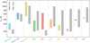Fig. 9

Range in excitation temperatures (shaded colored areas) for all detected species measured toward the embedded low-mass protostellar systems in the JOYS sample. For each species, the range measured toward high-mass sources is presented in the shaded gray areas (Boogert et al. 1998; Lahuis & van Dishoeck 2000; Keane et al. 2001; Boonman et al. 2003; Knez et al. 2009; Karska et al. 2014; Dungee et al. 2018; Barr et al. 2018, 2020; Nickerson et al. 2023; Francis et al. 2024). Since for no data are available for SiO and C₄H₂ in high-mass sources, these are not displayed.

5 Summary

This paper presents an overview of molecular emission and absorption features detected in JWST/MIRI-MRS observations of the sample of 18 low-mass protostars in the JOYS program. The spectra of the central regions of 16 sources where mid-IR continuum was detected were fit using LTE slab models to determine the physical conditions in which the molecules reside. This includes molecules such as CO₂, C₂H₂, and CH₄ that cannot be studied at millimeter wavelengths. Abundance ratios were derived with respect to H₂O, and together with the derived excitation conditions were used to determine the origin of the molecular emission and absorption features. Based on the aforementioned analysis, our main conclusions are as follows:

The spectra show an unprecedented richness in molecular emission and absorption features. Molecular features can be either in absorption against the bright embedded IR continuum (e.g., B1-c) or in emission (e.g., L1448-mm);
Water is the most commonly detected species in the MIRI-MRS observations, being present in 12/16 sources. Almost similarly present are CO₂ (11/16), CO (8/16), and OH (7/16). All other molecules are detected in at most three sources (predominantly B1-c and L1448-mm); these include ¹³CO₂, C₂H₂, ¹³CCH₂, HCN, C₄H₂, CH₄, and SO₂;
The data yield the surprising detection of SiO toward L1448-mm (emission) and BHR71-IRS1 (absorption) and, for the first time, CS and NH₃ at mid-IR wavelengths toward a low-mass protostellar source (B1-c);
The excitation temperatures derived toward the majority of the species lie in the 100-300 K range, consistent with those derived toward high-mass sources but significantly lower than what is typically observed toward more evolved Class II disks;
For sources showing molecules in emission, IR pumping has to be taken into account in deriving accurate column densities and the total number of molecules;
Molecular emission and absorption features in embedded protostellar systems can trace various components. The abundance ratios with respect to H₂O are fully consistent with ice sublimation toward the famous hot core source B1-c and, to a lesser extent, in several other sources (e.g., Ser-SMM1B). On the other hand, the discrepancy between gas and ice abundances with respect to H₂O, together with the detection of SiO, suggest outflow shock origins toward L1448-mm and BHR71-IRS1. Also, the cold and velocity-shifted CO₂ emission toward several other sources (e.g., Ser-SMM3, Ser-S68N-N) is consistent with outflowing material;
The JOYS data yield surprisingly few detections of molecular gas in the hot inner regions of the disk. TMC1-W is the only source with both a confirmed embedded disk and detected hot (~1200 K) molecular emission (H₂O), with only two other sources showing such hot H₂O features. This is in strong contrast with the more evolved Class II sources where hot molecular features are detected for many species (CO₂, C₂H₂, HCN). The non-detection of a broader range of molecular features from the embedded disks likely originates from extinction due to unsettled dust grains in the upper layers of the disk.

The JOYS data have shown the great potential of detecting and characterizing molecular emission and absorption features toward embedded protostellar systems. The unprecedented spatial and spectral resolution and sensitivity of JWST/MIRI-MRS will certainly yield more beautiful and line-rich data of embedded protostellar systems, further enlightening us about the processes that take place on disk and outflow scales. Furthermore, additional work on modeling the structure of embedded systems, including the disk and outflow, as well as their evolution will further shed light on what the molecular features detected at mid-IR wavelengths are tracing and what the chemical composition is during the onset of planet formation.

Data availability

Appendices B-H are available online at https://doi.org/10.5281/zenodo.14097317.

Acknowledgements

We would like to thank the anonymous referee for their constructive comments on the manuscript and John Black for fruitful discussions on non-LTE effects and infrared pumping. This work is based on observations made with the NASA/ESA/CSA James Webb Space Telescope. The data were obtained from the Mikulski Archive for Space Telescopes at the Space Telescope Science Institute, which is operated by the Association of Universities for Research in Astronomy, Inc., under NASA contract NAS 5-03127 for JWST. These observations are associated with program #1290. The following National and International Funding Agencies funded and supported the MIRI development: NASA; ESA; Belgian Science Policy Office (BELSPO); Centre Nationale d’Études Spatiales (CNES); Danish National Space Centre; Deutsches Zentrum fur Luftund Raumfahrt (DLR); Enterprise Ireland; Ministerio De Economiá y Competividad; The Netherlands Research School for Astronomy (NOVA); The Netherlands Organisation for Scientific Research (NWO); Science and Technology Facilities Council; Swiss Space Office; Swedish National Space Agency; and UK Space Agency. MvG, LF, EvD, YC, KS, and WR acknowledge support from ERC Advanced grant 101019751 MOLDISK, TOP-1 grant 614.001.751 from the Dutch Research Council (NWO), The Netherlands Research School for Astronomy (NOVA), the Danish National Research Foundation through the Center of Excellence “InterCat” (DNRF150), and DFG-grant 325594231, FOR 2634/2. T.P.R. acknowledges support from ERC grant 743029 EASY. H.B. acknowledges support from the Deutsche Forschungsgemeinschaft in the Collaborative Research Center (SFB 881) “The Milky Way System” (subproject B1) A.C.G. acknowledges support from PRIN-MUR 2022 20228JPA3A “The path to star and planet formation in the JWST era (PATH)” funded by NextGeneration EU and by INAF-GoG 2022 “NIR-dark Accretion Outbursts in Massive Young stellar objects (NAOMY)” and Large Grant INAF 2022 “YSOs Outflows, Disks and Accretion: towards a global framework for the evolution of planet forming systems (YODA)”. KJ acknowledges the support from the Swedish National Space Agency. P.J.K. acknowledges support from the Science Foundation Ireland/Irish Research Council Pathway programme under Grant Number 21/PATH-S/9360. P.N. acknowledges support from the ESO Fellowship and IAU Gruber Foundation Fellowship programs. This research made use of NumPy (Harris et al. 2020); Astropy, a community-developed core Python package for Astronomy (Astropy Collaboration 2022); Matplotlib (Hunter 2007).

Appendix A LTE results per molecule

A.1 H₂O

As discussed in Sect. 3.3, H₂O is the most commonly detected molecule in the JOYS data. In total, three different components were used to fit all the water lines across the full MIRI-MRS wavelength range. For the rovibrational lines shortward of 10 µm, one warm component provided a good fit to the data (see e.g., Fig. 3 for TMC1-W). On the other hand, for the pure rotational lines longward of 10 µm, two components with two different temperatures were needed to provide an accurate fit to the data with typical temperatures of ~ 150 K and ~400 K, called cold and warm, respectively (see Table 2 and Fig. A.1). In all sources where two components were needed to fit the pure rotational emission, the cold H₂O components traces the bulk of the H₂O (i.e., a higher N or 𝒩_mol than the warm component).

In several sources, the rovibrational component appears to be tracing the same H₂O as the pure rotational lines. This is especially clear toward B1-c, the only source where both the rotational and rovibrational lines of H₂O (and those of other species) are detected solely in absorption. The excitation temperature derived from the pure rotational lines (325 ± 15 K) is in perfect agreement with that derived from the rovibrational lines (300 ± 10 K) and also the column densities are within error bars in good agreement (4.4 ± 1.2 × 10¹⁸ cm⁻² and 7.8 ± 2.2 × 10¹⁸ cm⁻², respectively; see Table H.4). This shows that there is one warm component of H₂O that is absorbing against the bright continuum across the full wavelength range.

Other sources with agreement between the excitation conditions of the rovibrational lines and the pure rotational lines are B1-a-NS and L1448-mm (see Table 2). Toward both of these sources, H₂O is present in emission and two components were needed to fit the pure rotational lines (see Fig. A.1). The rovibra-tional lines in B1-a-NS seem to be tracing the same gas as the warm component of H₂O (~400 K) with an additional cold component of 160 ± 10 K traced by the lower E_up rotational lines. On the other hand, toward L1448-mm the temperature derived from the rovibrational lines (180 ± 10 K) is in better agreement with the cold H₂O component of the rotational lines (130 ± 10 K) than with the warm rotational H₂O component (390 ± 10 K) which is clearly tracing warmer gas.

Interestingly, toward the TMC1 binary, the rovibrational lines are in absorption toward TMC1-E (see Fig. G.25) whereas they are in emission toward TMC1-W (see Fig. 3). The pure rotational lines are in emission (see Figs. G.26 and G.28), but at these wavelengths the two components of the binary are barely resolved so it is not possible to determine which of the two components (or both) is showing this H₂O in emission. The excitation temperature of the rovibrational lines between the two components is very different with TMC1-W showing much hotter H₂O than TMC1-E (1280 ± 20 K and 580 ± 20 K, respectively). The radius of the emitting area derived for TMC1-W is 0.06 ± 0.01 au, consistent with a hot inner disk, whereas for TMC1-E no emitting area can be derived since the rovibrational lines are in absorption. In contrast, the radii of the emitting areas derived from the pure rotational lines are 0.3 ± 0.1 au (warm component) and 6.4 ± 1.9 au (cold component), suggesting that these are tracing more extended H₂O emission. Similarly to TMC1, the rovibrational lines of H₂O are in absorption toward BHR71-IRS1 whereas the rotational lines are in emission. The temperatures between these two components are significantly different (560 ± 10 K and 140 ± 10 K, respectively). The emitting area derived for the cold component is 24 ± 1 au, which is consistent with it being present on larger scales in the system (e.g., outflow), although it remains spatially unresolved at the continuum position. For the rovibrational lines, no emitting area can be derived since the lines are in absorption, but the velocity offset for both H₂O components (−42 ± 3 km s⁻¹ and −44 ± 9 km s⁻¹, respectively) is consistent with outflowing material.

In multiple sources (e.g., SVS 4-5, TMC1-E, TMC1-W), all water components are tracing three distinct physical components, where the rovibrational lines trace the hottest component. The majority of the H₂O in all sources resides at temperatures of ≲ 600 K. However, toward a few sources (i.e., Ser-SMM1B, SVS4-5, TMC1-W) very hot water with temperatures of up to 1200 K is detected. Toward TMC1-W and SVS4-5, this hot water is seen in emission (see Fig. 3) whereas toward Ser-SMM1B it is seen in absorption. This hot water component is similar to that found in Class II disks (e.g., Banzatti et al. 2023a; Perotti et al. 2023; Pontoppidan et al. 2024; Temmink et al. 2024a) and likely originates from the inner disk close to the protostar where the temperatures are high enough to produce such hot water.

A.2 CO₂

For L1448-mm, the best-fit models of CO₂, C₂H₂, HCN, and C₄H₂ are presented in Fig. A.2. As was mentioned in Sect. 3.3, CO₂ is the second most detected molecule next to H₂O. It seems to be tracing rather cold regions in embedded protostellar systems (see Table 2). Typical temperatures are about ~200 K, with the highest temperature of 315 ± 25 K measured toward TMC1-E and the lowest temperature of 60 ± 10 K measured toward TMC1A. This is in strong contrast to what is seen toward more evolved Class II disks where temperatures are typically much higher (> 500 K; Grant et al. 2023), although Class II disks with lower temperature CO₂ also exist (e.g., Schwarz et al. 2024). The abundance ratios with respect to H₂O (derived from the cold and warm components of the pure rotational lines) suggest a range of abundances from 10⁻⁵ − 10⁻¹ due to the effect of infrared pumping.

In several cases, the lines of CO₂ are blueshifted (i.e., BHR71-IRS1, SVS4-5) or even redshifted (i.e., B1-a-NS, Ser-SMM1B) by up to several tens of km s⁻¹, suggesting that it is either located in the outflow or is infalling. A clear case where CO₂ (as well as other molecular species) is tracing outflowing material is BHR71-IRS1, where all lines of CO₂ are shifted by −10 ± 4 km s⁻¹ with respect to the υ_lsr and show some spatially extended emission along the outflow cavity walls. The velocity shift is similar but slightly lower than other species such as H₂O and SiO (−45 km s⁻¹ and −23 ± 2 km s⁻¹, respectively; see Table H.16). BHR71-IRS1 also shows strong and spatially extended H₂ and atomic lines that are blueshifted by similar velocities, which will be discussed in a separate paper (Tychoniec et al. in prep.). The CO₂ lines toward SVS4-5 are even shifted by −80 km s⁻¹, but these likely originate from the outflow of the nearby Class 0 source Ser-SMM4 (Pontoppidan et al. 2004). On the other hand, the absorption lines toward B1-a-NS are redshifted by 35 km s⁻¹ , which is consistent with either tracing the redshifted outflow or with infalling material. Some weak extended emission of CO₂ is present in the southern direction, which is indicates that an outflow origin is more likely. However, the S/N of the CO₂ is low and the lines are strongly blended with H₂O lines (see Fig. G.2), hampering a more precise analysis.

Toward B1-c and L1448-mm, also the ¹³CO₂ isotopolog is detected (see Figs. 2 and A.2). The excitation temperature measured for B1-c (220 ± 30 K) is very similar to that of CO₂ (270 ± 10 K), suggesting that they are tracing the same component. For L1448-mm, the excitation temperature cannot be accurately constrained below 300 K, and was therefore fixed to that of CO₂ (120 K). Adopting a typical ¹²C/¹³C ratio of 70 for the local ISM (Milam et al. 2005), the derived abundance ratio of CO₂ with respect to H₂O in B1-c is a factor of ~5 higher than derived directly from the main isotopolog, likely due to line optical depth effects of CO₂. For L1448-mm, the abundances of ¹³CO₂ multiplied by 70 and CO₂ itself agree perfectly, given that the Q branch is excluded from the fit (see Appendix E).

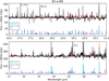Fig. A.1

Baseline-subtracted spectrum (black) and best-fit LTE model (shaded red) for B1-a-NS in the 16.5 – 27.5 µm range. At the bottom of each panel, the individual best-fit LTE models of cold H₂O (cyan), warm H₂O (blue), and OH (pink) are shown at an arbitrary constant offset. Deep negative absorption features originating from detector artifacts are clipped for clarity.

A.3 C₂H₂

Acetylene is detected toward three sources, B1-c, L1448-mm, and BHR71-IRS1 through its V5 bending mode around 13.6 µm (see e.g., Figs. 2 and A.2). The derived excitation temperatures are 300 ± 10 K and 110 ± 10 K for B1-c and L1448-mm, respectively (see Table 2). For BHR71-IRS1, the excitation temperature could not be constrained since only the Q branch is weakly detected and was fixed to 150 K. This is significantly lower than what is typically observed toward more evolved Class II sources (≿ 500 K; e.g., Salyk et al. 2011; Grant et al. 2023; Tabone et al. 2023; Arabhavi et al. 2024). Interestingly, the excitation temperature of ¹³CCH₂ (140 ± 30 K) is lower than that of C₂H₂ for B1-c, suggesting that ¹³CCH₂ might be probing a different region than the main isotopolog. However, the temperature of the main isotopolog may also be overestimated due to line optical depth effects (e.g., Appendix E, Li et al. 2024), even though the optically thick Q branch was excluded from the fit. Furthermore, the lines of ¹³CCH₂ are blended with those of C₂H₂ and HCN (see e.g., Fig. 2), which are much stronger, hampering the analysis of ¹³CCH₂.

The high optical depth of the C₂H₂ lines is further supported by the ratios of the column densities for B1-c. The derived column density ratio with respect to H₂O is about a factor of -7 higher than derived directly from C₂H₂ when adopting a ¹²C/¹³C ratio of 70 (Milam et al. 2005). For L1448-mm, the ratio of ¹³CCH₂ is in perfect agreement with C₂H₂ if the Q branch of the latter is excluded from the fit (see Appendix E). The effect of IR pumping is only a factor of a few given that the derived excitation temperature of C₂H₂ (110 ± 10 K) is only slightly lower than the brightness temperature at 7.7 µm (118 K). The ratio of C₂H₂/CO₂ is similar between B1-c and L1448-mm, but in BHR71-IRS1 C₂H₂ appears to be almost two orders of magnitude less abundant than CO₂. However, given both the lack of ¹³CO₂ and ¹³CCH₂ detections toward this source and the fact that only the possibly optically thick Q branches are detected for CO₂ and C₂H₂, the effect of line optical depth cannot be excluded. The upper limit of ¹³CCH₂ is consistent with the ratio of C₂H₂/CO₂ in B1-c and L1448-mm.

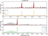Fig. A.2

Baseline-subtracted spectrum (black) and best-fit LTE model (shaded red) for L1448-mm in the 13.2 – 16.2 µm range. At the bottom of each panel, the individual best-fit LTE models of warm H₂O (blue), C₂H₂ (orange), ¹³CCH₂ (brown), HCN (yellow), CO₂ (green), ¹³CO₂ (purple), and C₄H₂ are shown at an arbitrary constant offset. Deep negative absorption features originating from detector artifacts are clipped for clarity.

A.4 HCN

Hydrogen cyanide is only detected in its ν₂ mode around 14 µm toward B1-c and L1448-mm (see Figs. 2 and A.2). Interestingly, similar temperatures are derived from its ν2 mode around 14 µm as for ¹³CCH₂ in both B1-c (180 ± 10 K) and C₂H₂ in L1448-mm (110 ± 10 K). This likely means that they are located in the same component of the protostellar system. Similarly to C₂ H₂, the derived excitation temperatures are significantly lower than commonly observed toward more evolved Class II sources. Furthermore, the abundance ratios with respect to H₂O indicates that HCN is equally abundant as C₂H₂ in both B1-c (7.3 ± 2.9 × 10⁻²) and L1448-mm (1 × 10⁻³ − 2 × 10⁻²), although for the latter source the effect of IR pumping provides an order of magnitude uncertainty. The uncorrected abundance of HCN is ~2 × 10⁻², which would make it almost similarly abundant with respect to H₂O as C₂H₂.

A.5 C₄H₂

Toward L1448-mm, also C₄H₂ is detected in emission through the Q branch of its ν₈ bending mode at 15.92 µm (see Fig. A.2). Its excitation temperature cannot be accurately constrained and was therefore fixed to 100 K, but any temperatures higher than 150 K can be excluded from the shape of the Q branch. Similarly to C₂H₂ and HCN, the derived upper limit on T_ex is significantly lower than in Class II sources. The abundance with respect to H₂O (~10⁻⁴ − 10⁻³) is about an order of magnitude lower than C₂H₂ and HCN, which is also consistent with the upper limit derived for B1-c (< 2 × 10⁻⁴) and other sources.

A.6 CH₄

The best-fit LTE model of CH₄ in L1448-mm is presented in the top panel of Fig. 4. The ν₄ mode of CH₄ is clearly detected through its Q branch at 7.66 µm, as well as through the R and P branch lines on either sides. The CH₄ features mildly suffer from extinction due to the (rather narrow) ice absorption band of CH₄ at 7.67 µm which also hampered the continuum determination. This differential extinction is taken into account in the LTE slab model fits but has only minor effects on the results. Besides B1-c and L1448-mm, CH₄ is also detected (weakly) in emission toward SVS4-5. The excitation temperatures derived for all three sources vary significantly (see Table 2), with L1448-mm and B1-c showing a much lower excitation temperatures (130 ± 10 K and 200 ± 10 K, respectively) compared to SVS4-5 (460 ± 80 K). However, as for CO₂, the absorption of CH₄ in SVS4-5 likely originates from the outflow of Ser-SMM4 in front of SVS4-5 given the high blueshifted velocity of −40 km s⁻¹. Methane thus shows similarly low temperatures between 100 – 200 K to the other molecules toward the protostellar positions. For B1-c, the derived ratio with respect to H₂O (9.7 ± 3.8 × 10⁻²) is similar to C₂H₂ and HCN and about a factor of two lower than CO₂. On the other hand, the abundance with respect to H₂O is almost an order of magnitude higher (0.62 ± 0.09) toward L1448-mm, making it only a factor of two less abundant than H₂O.

A.7 SO₂

Sulfur-dioxide is only detected toward B1-c and L1448-mm through its ν₃ asymmetric stretching mode around 7.35 µm (see Figs. 2 and 4), whereas its ν₁ symmetric stretching mode around 9 µm and ν₂ bending mode around 19 µm are both not detected. The absence of the ν₁ and ν₂ modes in B1-c is consistent with the best-fit LTE model, but according to the best-fit LTE model of L1448-mm the ν₁ and ν₂ modes should have been easily detected. This suggests that IR pumping through the ν₃ band could be important in L1448-mm similarly to the low-mass sources NGC 1333 IRAS 2A (van Gelder et al. 2024), consistent with other molecules such as CO₂ in this source (see e.g., Sect. A.2). The derived temperatures for B1-c (135 ± 25 K) and L1448-mm (115 ± 15 K) are very similar to that derived for IRAS 2A (95 ± 10 K; van Gelder et al. 2024). The abundance of SO₂ with respect to H₂O in B1-c is 1.3 ± 0.5 × 10⁻², which is about one order of magnitude lower than CO₂, C₂H₂, HCN, and CH₄. For L1448-mm, the range of SO₂ abundances is 0.03 − 4 when taking IR pumping into account.

A.8 CS

Toward B1-c, CS is seen in absorption through its ν₂ mode between 7.5 − 8.5 µm (see Figs. 2 and 5). Carbon monosulfide has so far only been detected in absorption toward high-mass protostellar systems (e.g., Knez et al. 2009; Barr et al. 2018; Nickerson et al. 2023) but never at mid-IR wavelengths toward a low-mass sources. The R branch lines are severely blended with the P branch lines of CH₄ and were therefore excluded in the fit, but P branch of CS shows clear unblended transitions. The excitation temperature of 285 ± 15 K is in very good agreement with other molecules toward B1-c (see Table 2), suggesting it is tracing the same gas. The derived abundance ratio of 5.5 ± 2.1 × 10⁻² is consistent with that of C₂H₂, HCN, and CH₄ and a factor of ~5 higher than that of SO₂.

A.9 SiO

Silicon monoxide is detected through its ν₁ mode in emission toward L1448-mm and in absorption toward BHR71-IRS1 (see Fig. 4). Thus far, SiO has only been detected at mid-IR wavelengths in absorption toward low-mass protostellar systems in the disk around an outbursting protostar (McClure et al. 2024). Here, the R and P branches are clearly detected between 7.8 µm and 8.5 µm and well fit with the LTE models. The derived excitation temperatures are similar for the two sources, 305 ± 15 K and 405 ± 25 K for L1448-mm and BHR71-IRS1, respectively. This is much lower than the temperature needed for thermal sublimation of silicon grains (~1500 K), implying that the SiO is not located within the dust sublimation radius. A likely origin is that the SiO is located in inner jet shocks where the silicon is sputtered off the dust grains in the shocks. This is further supported by blueshifted velocities of −24 ± 2 km s⁻¹ and −23 ± 2 km s⁻¹ with respect to the υ_lsr of the SiO lines and the emitting area of 1.9 ± 0.3 au derived for L1448-mm, pointing toward shocked regions in the inner jet or outflow. Furthermore, both L1448-mm and BHR71-IRS1 show very prominent outflows (e.g., Guilloteau et al. 1992; Tobin et al. 2018; Nazari et al. 2024b; Gavino et al. 2024) and in particular L1448-mm hosts a collimated high-velocity jet traced by SiO at millimeter wavelengths (Jiménez-Serra et al. 2011; Podio et al. 2021; Tychoniec et al. 2021; Nazari et al. 2024b).

The abundance ratios with respect to H₂O is 2.0 ± 0.6 × 10⁻⁴ in L1448-mm, which is three orders of magnitude lower than CH₄ and the minimum abundance of CO₂ and consistent with the range of C₄H₂. In contrast, the abundance ratio of SiO with respect to the rovibrational H₂O component in BHR71 IRS1 (the rotational lines are in emission) is much higher at 0.32 ± 0.13 which is two orders of magnitude higher than that of CO₂ (5.6 ± 2.2 × 10⁻³) and three orders of magnitude higher than that of C₂H₂ (1.8 ± 0.7 × 10⁻⁴). This suggests that especially in BHR71-IRS1, a lot of silicon is being released from the grains. The upper limit for B1-c is < 5.5 × 10⁻³, which is consistent with L1448-mm but two orders of magnitude lower than BHR71-IRS1.

A.10 NH₃

Another surprising detection is that of the NH₃ ν₂ symmetric bending mode in B1-c. This is, to the best of our knowledge, the first detection of NH₃ at mid-IR wavelengths toward a low-mass embedded protostellar system, with only a few detections toward high-mass sources (e.g., Evans et al. 1991; Barr et al. 2020; Nickerson et al. 2023). The best-fit LTE model is shown in Fig. 5. Clear absorption features of NH₃ are detected both between 8.2 µm and 9.3 µm, as well as longward of 10.2 µm, which are very well reproduced by the best-fit LTE model. The derived excitation temperature is 330 ± 10 K, which is consistent with those of CO₂ and H₂O (warm and rovibrational lines; see Table 2). Furthermore, the derived column density ratio with respect to H₂O is 4.1 ± 1.6 × 10⁻², which is very similar to almost all other molecules. However, the upper limits for several other sources are significantly lower (i.e., < 4 × 10⁻³ for L1448-mm).

References

ALMA Partnership (Brogan, C. L., et al.) 2015, ApJ, 808, L3 [Google Scholar]
Arabhavi, A. M., Kamp, I., Henning, T., et al. 2024, Science, 384, 1086 [NASA ADS] [CrossRef] [Google Scholar]
Arce, H. G., Borkin, M. A., Goodman, A. A., Pineda, J. E., & Halle, M. W. 2010, ApJ, 715, 1170 [NASA ADS] [CrossRef] [Google Scholar]
Argyriou, I., Glasse, A., Law, D. R., et al. 2023, A&A, 675, A111 [NASA ADS] [CrossRef] [EDP Sciences] [Google Scholar]
Assani, K. D., Harsono, D., Ramsey, J. P., et al. 2024, A&A, 688, A26 [NASA ADS] [CrossRef] [EDP Sciences] [Google Scholar]
Astropy Collaboration (Price-Whelan, A. M., et al.) 2022, ApJ, 935, 167 [NASA ADS] [CrossRef] [Google Scholar]
Avni, Y. 1976, ApJ, 210, 642 [NASA ADS] [CrossRef] [Google Scholar]
Bally, J. 2016, ARA&A, 54, 491 [Google Scholar]
Banzatti, A., Pontoppidan, K. M., Carr, J. S., et al. 2023a, ApJ, 957, L22 [NASA ADS] [CrossRef] [Google Scholar]
Banzatti, A., Pontoppidan, K. M., Pére Chávez, J., et al. 2023b, AJ, 165, 72 [CrossRef] [Google Scholar]
Barr, A. G., Boogert, A., DeWitt, C. N., et al. 2018, ApJ, 868, L2 [NASA ADS] [CrossRef] [Google Scholar]
Barr, A. G., Boogert, A., DeWitt, C. N., et al. 2020, ApJ, 900, 104 [NASA ADS] [CrossRef] [Google Scholar]
Barr, A. G., Boogert, A., Li, J., et al. 2022, ApJ, 935, 165 [NASA ADS] [CrossRef] [Google Scholar]
Beuther, H., van Dishoeck, E. F., Tychoniec, L., et al. 2023, A&A, 673, A121 [NASA ADS] [CrossRef] [EDP Sciences] [Google Scholar]
Bianchi, E., Chandler, C. J., Ceccarelli, C., et al. 2020, MNRAS, 498, L87 [NASA ADS] [CrossRef] [Google Scholar]
Bjerkeli, P., van der Wiel, M. H. D., Harsono, D., Ramsey, J. P., & Jørgensen, J. K. 2016, Nature, 540, 406 [Google Scholar]
Blake, G. A., & Boogert, A. C. A. 2004, ApJ, 606, L73 [NASA ADS] [CrossRef] [Google Scholar]
Boogert, A. C. A., Helmich, F. P., van Dishoeck, E. F., et al. 1998, A&A, 336, 352 [NASA ADS] [Google Scholar]
Boogert, A. C. A., Pontoppidan, K. M., Knez, C., et al. 2008, ApJ, 678, 985 [Google Scholar]
Boogert, A. C. A., Gerakines, P. A., & Whittet, D. C. B. 2015, ARA&A, 53, 541 [Google Scholar]
Boonman, A. M. S., & van Dishoeck, E. F. 2003, A&A, 403, 1003 [NASA ADS] [CrossRef] [EDP Sciences] [Google Scholar]
Boonman, A. M. S., van Dishoeck, E. F., Lahuis, F., et al. 2003, A&A, 399, 1047 [NASA ADS] [CrossRef] [EDP Sciences] [Google Scholar]
Bosman, A. D., Bruderer, S., & van Dishoeck, E. F. 2017, A&A, 601, A36 [NASA ADS] [CrossRef] [EDP Sciences] [Google Scholar]
Bottinelli, S., Ceccarelli, C., Lefloch, B., et al. 2004, ApJ, 615, 354 [Google Scholar]
Bruderer, S., Harsono, D., & van Dishoeck, E. F. 2015, A&A, 575, A94 [NASA ADS] [CrossRef] [EDP Sciences] [Google Scholar]
Brunken, N. G. C., van Dishoeck, E. F., Slavicinska, K., et al. 2024, A&A, 692, A163 [NASA ADS] [CrossRef] [EDP Sciences] [Google Scholar]
Bushouse, H., Eisenhamer, J., Dencheva, N., et al. 2024, https://doi.org/ 10.5281/zenodo.14153298 [Google Scholar]
Caratti o Garatti, A., Ray, T. P., Kavanagh, P. J., et al. 2024, A&A, 691, A134 [NASA ADS] [CrossRef] [EDP Sciences] [Google Scholar]
Carr, J. S., & Najita, J. R. 2008, Science, 319, 1504 [Google Scholar]
Carr, J. S., & Najita, J. R. 2014, ApJ, 788, 66 [NASA ADS] [CrossRef] [Google Scholar]
Caselli, P., & Ceccarelli, C. 2012, A&A Rev., 20, 56 [NASA ADS] [CrossRef] [Google Scholar]
Caselli, P., Hartquist, T. W., & Havnes, O. 1997, A&A, 322, 296 [NASA ADS] [Google Scholar]
Ceccarelli, C., Codella, C., Balucani, N., et al. 2023, in Astronomical Society of the Pacific Conference Series, 534, Protostars and Planets VII, eds. S. Inutsuka, Y. Aikawa, T. Muto, K. Tomida, & M. Tamura, 379 [NASA ADS] [Google Scholar]
Charnley, S. B. 1997, ApJ, 481, 396 [NASA ADS] [CrossRef] [Google Scholar]
Charnley, S. B., Tielens, A. G. G. M., & Millar, T. J. 1992, ApJ, 399, L71 [Google Scholar]
Chen, Y., van Gelder, M. L., Nazari, P., et al. 2023, A&A, 678, A137 [NASA ADS] [CrossRef] [EDP Sciences] [Google Scholar]
Chen, Y., Rocha, W. R. M., van Dishoeck, E. F., et al. 2024, A&A, 690, A205 [NASA ADS] [CrossRef] [EDP Sciences] [Google Scholar]
Choi, M. 2009, ApJ, 705, 1730 [Google Scholar]
Christiaens, V., Gonzalez, C., Farkas, R., et al. 2023, J. Open Source Softw., 8, 4774 [NASA ADS] [CrossRef] [Google Scholar]
Codella, C., Maury, A. J., Gueth, F., et al. 2014, A&A, 563, L3 [NASA ADS] [CrossRef] [EDP Sciences] [Google Scholar]
Coletta, A., Fontani, F., Rivilla, V. M., et al. 2020, A&A, 641, A54 [NASA ADS] [CrossRef] [EDP Sciences] [Google Scholar]
Cridland, A. J., Rosotti, G. P., Tabone, B., et al. 2022, A&A, 662, A90 [NASA ADS] [CrossRef] [EDP Sciences] [Google Scholar]
Dionatos, O., Nisini, B., Garcia Lopez, R., et al. 2009, ApJ, 692, 1 [NASA ADS] [CrossRef] [Google Scholar]
Dionatos, O., Jørgensen, J. K., Teixeira, P. S., Güdel, M., & Bergin, E. 2014, A&A, 563, A28 [NASA ADS] [CrossRef] [EDP Sciences] [Google Scholar]
Dullemond, C. P., & Dominik, C. 2005, A&A, 434, 971 [CrossRef] [EDP Sciences] [Google Scholar]
Dullemond, C. P., Hollenbach, D., Kamp, I., & D’Alessio, P. 2007, in Protostars and Planets V, eds. B. Reipurth, D. Jewitt, & K. Keil, 555 [Google Scholar]
Dungee, R., Boogert, A., DeWitt, C. N., et al. 2018, ApJ, 868, L10 [NASA ADS] [CrossRef] [Google Scholar]
Encalada, F. J., Looney, L. W., Takakuwa, S., et al. 2024, ApJ, 966, 32 [NASA ADS] [CrossRef] [Google Scholar]
Endres, C. P., Schlemmer, S., Schilke, P., Stutzki, J., & Müller, H. S. P. 2016, J. Mol. Spectrosc., 327, 95 [NASA ADS] [CrossRef] [Google Scholar]
Evans, I., Neal J., Lacy, J. H., & Carr, J. S. 1991, ApJ, 383, 674 [NASA ADS] [CrossRef] [Google Scholar]
Evans, I., Neal J., Dunham, M. M., Jørgensen, J. K., et al. 2009, ApJS, 181, 321 [NASA ADS] [CrossRef] [Google Scholar]
Federman, S. A., Megeath, S. T., Rubinstein, A. E., et al. 2024, ApJ, 966, 41 [CrossRef] [Google Scholar]
Fischer, W. J., Megeath, S. T., Furlan, E., et al. 2017, ApJ, 840, 69 [NASA ADS] [CrossRef] [Google Scholar]
Flores, C., Ohashi, N., Tobin, J. J., et al. 2023, ApJ, 958, 98 [NASA ADS] [CrossRef] [Google Scholar]
Francis, L., van Gelder, M. L., van Dishoeck, E. F., et al. 2024, A&A, 683, A249 [NASA ADS] [CrossRef] [EDP Sciences] [Google Scholar]
Frank, A., Ray, T. P., Cabrit, S., et al. 2014, in Protostars and Planets VI, eds. H. Beuther, R. S. Klessen, C. P. Dullemond, & T. Henning, 451 [Google Scholar]
Garrod, R. T., Jin, M., Matis, K. A., et al. 2022, ApJS, 259, 1 [NASA ADS] [CrossRef] [Google Scholar]
Gasman, D., van Dishoeck, E. F., Grant, S. L., et al. 2023, A&A, 679, A117 [NASA ADS] [CrossRef] [EDP Sciences] [Google Scholar]
Gavino, S., Jørgensen, J. K., Sharma, R., et al. 2024, ApJ, 974, 21 [NASA ADS] [CrossRef] [Google Scholar]
Gieser, C., Beuther, H., van Dishoeck, E. F., et al. 2023, A&A, 679, A108 [NASA ADS] [CrossRef] [EDP Sciences] [Google Scholar]
Gordon, I. E., Rothman, L. S., Hargreaves, R. J., et al. 2022, J. Quant. Spec. Radiat. Transf., 277, 107949 [NASA ADS] [CrossRef] [Google Scholar]
Grant, S. L., van Dishoeck, E. F., Tabone, B., et al. 2023, ApJ, 947, L6 [NASA ADS] [CrossRef] [Google Scholar]
Greenfield, P., & Miller, T. 2016, Astron. Comput., 16, 41 [NASA ADS] [Google Scholar]
Greenwood, A. J., Kamp, I., Waters, L. B. F. M., Woitke, P., & Thi, W. F. 2019, A&A, 631, A81 [NASA ADS] [CrossRef] [EDP Sciences] [Google Scholar]
Guilloteau, S., Bachiller, R., Fuente, A., & Lucas, R. 1992, A&A, 265, L49 [NASA ADS] [Google Scholar]
Gupta, A., Miotello, A., Manara, C. F., et al. 2023, A&A, 670, L8 [NASA ADS] [CrossRef] [EDP Sciences] [Google Scholar]
Gusdorf, A., Cabrit, S., Flower, D. R., & Pineau Des Forêts, G. 2008a, A&A, 482, 809 [NASA ADS] [CrossRef] [EDP Sciences] [Google Scholar]
Gusdorf, A., Pineau Des Forêts, G., Cabrit, S., & Flower, D. R. 2008b, A&A, 490, 695 [NASA ADS] [CrossRef] [EDP Sciences] [Google Scholar]
Gusdorf, A., Giannini, T., Flower, D. R., et al. 2011, A&A, 532, A53 [CrossRef] [EDP Sciences] [Google Scholar]
Gusdorf, A., Riquelme, D., Anderl, S., et al. 2015, A&A, 575, A98 [CrossRef] [EDP Sciences] [Google Scholar]
Harris, C. R., Millman, K. J., van der Walt, S. J., et al. 2020, Nature, 585, 357 [NASA ADS] [CrossRef] [Google Scholar]
Harsono, D., Jørgensen, J. K., van Dishoeck, E. F., et al. 2014, A&A, 562, A77 [NASA ADS] [CrossRef] [EDP Sciences] [Google Scholar]
Harsono, D., Bjerkeli, P., van der Wiel, M. H. D., et al. 2018, Nat. Astron., 2, 646 [Google Scholar]
Harsono, D., Bjerkeli, P., Ramsey, J. P., et al. 2023, ApJ, 951, L32 [NASA ADS] [CrossRef] [Google Scholar]
Hatchell, J., Fuller, G. A., & Richer, J. S. 2007, A&A, 472, 187 [NASA ADS] [CrossRef] [EDP Sciences] [Google Scholar]
Helmich, F. P. 1996, PhD thesis, Leiden University, The Netherlands [Google Scholar]
Helmich, F. P., van Dishoeck, E. F., Black, J. H., et al. 1996, A&A, 315, L173 [NASA ADS] [Google Scholar]
Henning, T., Kamp, I., Samland, M., et al. 2024, PASP, 136, 054302 [NASA ADS] [CrossRef] [Google Scholar]
Herczeg, G. J., Brown, J. M., van Dishoeck, E. F., & Pontoppidan, K. M. 2011, A&A, 533, A112 [NASA ADS] [CrossRef] [EDP Sciences] [Google Scholar]
Herczeg, G. J., Karska, A., Bruderer, S., et al. 2012, A&A, 540, A84 [NASA ADS] [CrossRef] [EDP Sciences] [Google Scholar]
Hunter, J. D. 2007, Comput. Sci. Eng., 9, 90 [NASA ADS] [CrossRef] [Google Scholar]
Indriolo, N., Neufeld, D. A., Barr, A. G., et al. 2020, ApJ, 894, 107 [NASA ADS] [CrossRef] [Google Scholar]
Jiménez-Serra, I., Martín-Pintado, J., Winters, J. M., Rodríguez-Franco, A., & Caselli, P. 2011, ApJ, 739, 80 [CrossRef] [Google Scholar]
Jones, O. C., Álvarez-Márquez, J., Sloan, G. C., et al. 2023, MNRAS, 523, 2519 [Google Scholar]
Jørgensen, J. K., Schöier, F. L., & van Dishoeck, E. F. 2002, A&A, 389, 908 [CrossRef] [EDP Sciences] [Google Scholar]
Jørgensen, J. K., Harvey, P. M., Evans, I., Neal J., et al. 2006, ApJ, 645, 1246 [CrossRef] [Google Scholar]
Jørgensen, J. K., van der Wiel, M. H. D., Coutens, A., et al. 2016, A&A, 595, A117 [Google Scholar]
Jørgensen, J. K., Belloche, A., & Garrod, R. T. 2020, ARA&A, 58, 727 [Google Scholar]
Kalyaan, A., Pinilla, P., Krijt, S., Mulders, G. D., & Banzatti, A. 2021, ApJ, 921, 84 [CrossRef] [Google Scholar]
Kalyaan, A., Pinilla, P., Krijt, S., et al. 2023, ApJ, 954, 66 [NASA ADS] [CrossRef] [Google Scholar]
Karska, A., Herpin, F., Bruderer, S., et al. 2014, A&A, 562, A45 [NASA ADS] [CrossRef] [EDP Sciences] [Google Scholar]
Keane, J. V., Boonman, A. M. S., Tielens, A. G. G. M., & van Dishoeck, E. F. 2001, A&A, 376, L5 [NASA ADS] [CrossRef] [EDP Sciences] [Google Scholar]
Knez, C., Lacy, J. H., Evans, I., Neal J., van Dishoeck, E. F., & Richter, M. J. 2009, ApJ, 696, 471 [NASA ADS] [CrossRef] [Google Scholar]
Kóspál, Á., Ábrahám, P., Diehl, L., et al. 2023, ApJ, 945, L7 [CrossRef] [Google Scholar]
Kristensen, L. E., van Dishoeck, E. F., Bergin, E. A., et al. 2012, A&A, 542, A8 [NASA ADS] [CrossRef] [EDP Sciences] [Google Scholar]
Labiano, A., Argyriou, I., Álvarez-Márquez, J., et al. 2021, A&A, 656, A57 [NASA ADS] [CrossRef] [EDP Sciences] [Google Scholar]
Lacy, J. H., Evans, I., Neal J., Achtermann, J. M., et al. 1989, ApJ, 342, L43 [NASA ADS] [CrossRef] [Google Scholar]
Lacy, J. H., Carr, J. S., Evans, I., Neal J., et al. 1991, ApJ, 376, 556 [NASA ADS] [CrossRef] [Google Scholar]
Lahuis, F., & van Dishoeck, E. F. 2000, A&A, 355, 699 [NASA ADS] [Google Scholar]
Lahuis, F., van Dishoeck, E. F., Jørgensen, J. K., Blake, G. A., & Evans, N. J. 2010, A&A, 519, A3 [NASA ADS] [CrossRef] [EDP Sciences] [Google Scholar]
Law, D. D., Morrison, J. E., Argyriou, I., et al. 2023, AJ, 166, 45 [NASA ADS] [CrossRef] [Google Scholar]
Lee, C.-F., Ho, P. T. P., Li, Z.-Y., et al. 2017, Nat. Astro., 1, 0152 [NASA ADS] [CrossRef] [Google Scholar]
Lee, J.-E., Kim, C.-H., Lee, S., et al. 2024, ApJ, 966, 119 [NASA ADS] [CrossRef] [Google Scholar]
Leurini, S., Gusdorf, A., Wyrowski, F., et al. 2014, A&A, 564, L11 [NASA ADS] [CrossRef] [EDP Sciences] [Google Scholar]
Li, J., Boogert, A., & Tielens, A. G. G. M. 2024, ApJS, 273, 32 [NASA ADS] [CrossRef] [Google Scholar]
Lin, Z.-Y. D., Li, Z.-Y., Tobin, J. J., et al. 2023, ApJ, 951, 9 [NASA ADS] [CrossRef] [Google Scholar]
Maret, S., Bergin, E. A., Neufeld, D. A., et al. 2009, ApJ, 698, 1244 [NASA ADS] [CrossRef] [Google Scholar]
McClure, M. 2009, ApJ, 693, L81 [NASA ADS] [CrossRef] [Google Scholar]
McClure, M., Francis, L., van Dishoeck, E., et al. 2024, Nature, submitted [Google Scholar]
Meijerink, R., Pontoppidan, K. M., Blake, G. A., Poelman, D. R., & Dullemond, C. P. 2009, ApJ, 704, 1471 [Google Scholar]
Milam, S. N., Savage, C., Brewster, M. A., Ziurys, L. M., & Wyckoff, S. 2005, ApJ, 634, 1126 [Google Scholar]
Müller, H. S. P., Thorwirth, S., Roth, D. A., & Winnewisser, G. 2001, A&A, 370, L49 [Google Scholar]
Müller, H. S. P., Schlöder, F., Stutzki, J., & Winnewisser, G. 2005, J. Mol. Struct., 742, 215 [Google Scholar]
Narang, M., Manoj, P., Tyagi, H., et al. 2024, ApJ, 962, L16 [NASA ADS] [CrossRef] [Google Scholar]
Nazari, P., van Gelder, M. L., van Dishoeck, E. F., et al. 2021, A&A, 650, A150 [EDP Sciences] [Google Scholar]
Nazari, P., Meijerhof, J. D., van Gelder, M. L., et al. 2022, A&A, 668, A109 [NASA ADS] [CrossRef] [EDP Sciences] [Google Scholar]
Nazari, P., Cheung, J. S. Y., Asensio, J. F., et al. 2024a, A&A, 686, A59 [NASA ADS] [CrossRef] [EDP Sciences] [Google Scholar]
Nazari, P., Tabone, B., Ahmadi, A., et al. 2024b, A&A, 686, A201 [NASA ADS] [CrossRef] [EDP Sciences] [Google Scholar]
Neufeld, D. A., Manoj, P., Tyagi, H., et al. 2024, ApJ, 966, L22 [NASA ADS] [CrossRef] [Google Scholar]
Nickerson, S., Rangwala, N., Colgan, S. W. J., et al. 2023, ApJ, 945, 26 [NASA ADS] [CrossRef] [Google Scholar]
Nisini, B., Santangelo, G., Antoniucci, S., et al. 2013, A&A, 549, A16 [NASA ADS] [CrossRef] [EDP Sciences] [Google Scholar]
Öberg, K. I., Boogert, A. C. A., Pontoppidan, K. M., et al. 2008, ApJ, 678, 1032 [Google Scholar]
Ohashi, N., Tobin, J. J., Jørgensen, J. K., et al. 2023, ApJ, 951, 8 [NASA ADS] [CrossRef] [Google Scholar]
Oya, Y., López-Sepulcre, A., Sakai, N., et al. 2019, ApJ, 881, 112 [Google Scholar]
Pascucci, I., Cabrit, S., Edwards, S., et al. 2023, in Astronomical Society of the Pacific Conference Series, 534, Protostars and Planets VII, eds. S. Inutsuka, Y. Aikawa, T. Muto, K. Tomida, & M. Tamura, 567 [NASA ADS] [Google Scholar]
Perotti, G., Rocha, W. R. M., Jørgensen, J. K., et al. 2020, A&A, 643, A48 [EDP Sciences] [Google Scholar]
Perotti, G., Christiaens, V., Henning, T., et al. 2023, Nature, 620, 516 [NASA ADS] [CrossRef] [Google Scholar]
Podio, L., Codella, C., Gueth, F., et al. 2016, A&A, 593, L4 [NASA ADS] [CrossRef] [EDP Sciences] [Google Scholar]
Podio, L., Garufi, A., Codella, C., et al. 2020, A&A, 642, L7 [NASA ADS] [CrossRef] [EDP Sciences] [Google Scholar]
Podio, L., Tabone, B., Codella, C., et al. 2021, A&A, 648, A45 [NASA ADS] [CrossRef] [EDP Sciences] [Google Scholar]
Pontoppidan, K. M., van Dishoeck, E. F., & Dartois, E. 2004, A&A, 426, 925 [NASA ADS] [CrossRef] [EDP Sciences] [Google Scholar]
Pontoppidan, K. M., Boogert, A. C. A., Fraser, H. J., et al. 2008, ApJ, 678, 1005 [NASA ADS] [CrossRef] [Google Scholar]
Pontoppidan, K. M., Salyk, C., Banzatti, A., et al. 2024, ApJ, 963, 158 [NASA ADS] [CrossRef] [Google Scholar]
Ramírez-Tannus, M. C., Bik, A., Cuijpers, L., et al. 2023, ApJ, 958, L30 [CrossRef] [Google Scholar]
Ray, T. P., McCaughrean, M. J., Caratti o Garatti, A., et al. 2023, Nature, 622, 48 [NASA ADS] [CrossRef] [Google Scholar]
Rieke, G. H., Wright, G. S., Böker, T., et al. 2015, PASP, 127, 584 [NASA ADS] [CrossRef] [Google Scholar]
Rocha, W. R. M., van Dishoeck, E. F., Ressler, M. E., et al. 2024, A&A, 683, A124 [NASA ADS] [CrossRef] [EDP Sciences] [Google Scholar]
Rubinstein, A. E., Evans, N. J., Tyagi, H., et al. 2024, ApJ, 974, 112 [NASA ADS] [CrossRef] [Google Scholar]
Salyk, C., Pontoppidan, K. M., Blake, G. A., Najita, J. R., & Carr, J. S. 2011, ApJ, 731, 130 [Google Scholar]
Salyk, C., Yang, Y.-L., Pontoppidan, K. M., et al. 2024, ApJ, 974, 97 [NASA ADS] [CrossRef] [Google Scholar]
Schöier, F. L., van der Tak, F. F. S., van Dishoeck, E. F., & Black, J. H. 2005, A&A, 432, 369 [Google Scholar]
Schwarz, K. R., Henning, T., Christiaens, V., et al. 2024, ApJ, 962, 8 [NASA ADS] [CrossRef] [Google Scholar]
Segura-Cox, D. M., Schmiedeke, A., Pineda, J. E., et al. 2020, Nature, 586, 228 [NASA ADS] [CrossRef] [Google Scholar]
Sheehan, P. D., Tobin, J. J., Federman, S., Megeath, S. T., & Looney, L. W. 2020, ApJ, 902, 141 [Google Scholar]
Slavicinska, K., Boogert, A. C. A., Tychoniec, Ł., et al. 2024, A&A, in press, https://doi.org/10.1051/0004-6361/202451383 [Google Scholar]
Sonnentrucker, P., González-Alfonso, E., Neufeld, D. A., et al. 2006, ApJ, 650, L71 [CrossRef] [Google Scholar]
Sonnentrucker, P., González-Alfonso, E., & Neufeld, D. A. 2007, ApJ, 671, L37 [NASA ADS] [CrossRef] [Google Scholar]
Sturm, J. A., McClure, M. K., Beck, T. L., et al. 2023, A&A, 679, A138 [NASA ADS] [CrossRef] [EDP Sciences] [Google Scholar]
Suutarinen, A. N., Kristensen, L. E., Mottram, J. C., Fraser, H. J., & van Dishoeck, E. F. 2014, MNRAS, 440, 1844 [Google Scholar]
Tabone, B., van Hemert, M. C., van Dishoeck, E. F., & Black, J. H. 2021, A&A, 650, A192 [NASA ADS] [CrossRef] [EDP Sciences] [Google Scholar]
Tabone, B., Rosotti, G. P., Cridland, A. J., Armitage, P. J., & Lodato, G. 2022a, MNRAS, 512, 2290 [NASA ADS] [CrossRef] [Google Scholar]
Tabone, B., Rosotti, G. P., Lodato, G., et al. 2022b, MNRAS, 512, L74 [NASA ADS] [CrossRef] [Google Scholar]
Tabone, B., Bettoni, G., van Dishoeck, E. F., et al. 2023, Nat. Astron., 7, 805 [NASA ADS] [CrossRef] [Google Scholar]
Tabone, B., van Dishoeck, E. F., & Black, J. H. 2024, A&A, 691, A11 [NASA ADS] [CrossRef] [EDP Sciences] [Google Scholar]
Temmink, M., van Dishoeck, E. F., Gasman, D., et al. 2024a, A&A, 689, A330 [NASA ADS] [CrossRef] [EDP Sciences] [Google Scholar]
Temmink, M., van Dishoeck, E. F., Grant, S. L., et al. 2024b, A&A, 686, A117 [NASA ADS] [CrossRef] [EDP Sciences] [Google Scholar]
Thi, W. F., van Dishoeck, E. F., Pontoppidan, K. M., & Dartois, E. 2010, MNRAS, 406, 1409 [Google Scholar]
Tobin, J. J., & Sheehan, P. D. 2024, ARA&A, 62, 203 [NASA ADS] [CrossRef] [Google Scholar]
Tobin, J. J., Hartmann, L., Chiang, H.-F., et al. 2012, Nature, 492, 83 [NASA ADS] [CrossRef] [Google Scholar]
Tobin, J. J., Bergin, E. A., Hartmann, L., et al. 2013, ApJ, 765, 18 [NASA ADS] [CrossRef] [Google Scholar]
Tobin, J. J., Looney, L. W., Li, Z.-Y., et al. 2016, ApJ, 818, 73 [CrossRef] [Google Scholar]
Tobin, J. J., Looney, L. W., Li, Z.-Y., et al. 2018, ApJ, 867, 43 [CrossRef] [Google Scholar]
Toledano-Juárez, I., de la Fuente, E., Trinidad, M. A., Tafoya, D., & Nigoche-Netro, A. 2023, MNRAS, 522, 1591 [CrossRef] [Google Scholar]
Tychoniec, Ł., Tobin, J. J., Karska, A., et al. 2018, ApJS, 238, 19 [Google Scholar]
Tychoniec, Ł., Hull, C. L. H., Kristensen, L. E., et al. 2019, A&A, 632, A101 [NASA ADS] [CrossRef] [EDP Sciences] [Google Scholar]
Tychoniec, Ł., Manara, C. F., Rosotti, G. P., et al. 2020, A&A, 640, A19 [NASA ADS] [CrossRef] [EDP Sciences] [Google Scholar]
Tychoniec, Ł., van Dishoeck, E. F., van’t Hoff, M. L. R., et al. 2021, A&A, 655, A65 [NASA ADS] [CrossRef] [EDP Sciences] [Google Scholar]
Tychoniec, Ł., van Gelder, M. L., van Dishoeck, E. F., et al. 2024, A&A, 687, A36 [NASA ADS] [CrossRef] [EDP Sciences] [Google Scholar]
van der Tak, F. F. S., Black, J. H., Schöier, F. L., Jansen, D. J., & van Dishoeck, E. F. 2007, A&A, 468, 627 [NASA ADS] [CrossRef] [EDP Sciences] [Google Scholar]
van der Tak, F. F. S., Lique, F., Faure, A., Black, J. H., & van Dishoeck, E. F. 2020, Atoms, 8, 15 [Google Scholar]
van Dishoeck, E. F. 2004, ARA&A, 42, 119 [NASA ADS] [CrossRef] [Google Scholar]
van Dishoeck, E. F., & Blake, G. A. 1998, ARA&A, 36, 317 [Google Scholar]
van Dishoeck, E. F., Kristensen, L. E., Mottram, J. C., et al. 2021, A&A, 648, A24 [NASA ADS] [CrossRef] [EDP Sciences] [Google Scholar]
van Dishoeck, E. F., Grant, S., Tabone, B., et al. 2023, Faraday Discuss., 245, 52 [NASA ADS] [CrossRef] [Google Scholar]
van Gelder, M. L., Tabone, B., Tychoniec, Ł., et al. 2020, A&A, 639, A87 [NASA ADS] [CrossRef] [EDP Sciences] [Google Scholar]
van Gelder, M. L., Ressler, M. E., van Dishoeck, E. F., et al. 2024, A&A, 682, A78 [NASA ADS] [CrossRef] [EDP Sciences] [Google Scholar]
van’t Hoff, M. L. R., Tobin, J. J., Harsono, D., & van Dishoeck, E. F. 2018, A&A, 615, A83 [CrossRef] [EDP Sciences] [Google Scholar]
van’t Hoff, M. L. R., Harsono, D., Tobin, J. J., et al. 2020a, ApJ, 901, 166 [Google Scholar]
van’t Hoff, M. L. R., van Dishoeck, E. F., Jørgensen, J. K., & Calcutt, H. 2020b, A&A, 633, A7 [CrossRef] [EDP Sciences] [Google Scholar]
van’t Hoff, M. L. R., Tobin, J. J., Li, Z.-Y., et al. 2023, ApJ, 951, 10 [CrossRef] [Google Scholar]
Visser, R., van Dishoeck, E. F., Doty, S. D., & Dullemond, C. P. 2009, A&A, 495, 881 [NASA ADS] [CrossRef] [EDP Sciences] [Google Scholar]
Visser, R., Doty, S. D., & van Dishoeck, E. F. 2011, A&A, 534, A132 [NASA ADS] [CrossRef] [EDP Sciences] [Google Scholar]
Vlasblom, M., van Dishoeck, E. F., Tabone, B., & Bruderer, S. 2024, A&A, 682, A91 [NASA ADS] [CrossRef] [EDP Sciences] [Google Scholar]
Watson, D. M., Bohac, C. J., Hull, C., et al. 2007, Nature, 448, 1026 [NASA ADS] [CrossRef] [Google Scholar]
Wells, M., Pel, J. W., Glasse, A., et al. 2015, PASP, 127, 646 [NASA ADS] [CrossRef] [Google Scholar]
Woitke, P., Min, M., Thi, W. F., et al. 2018, A&A, 618, A57 [NASA ADS] [CrossRef] [EDP Sciences] [Google Scholar]
Wright, G. S., Wright, D., Goodson, G. B., et al. 2015, PASP, 127, 595 [NASA ADS] [CrossRef] [Google Scholar]
Wright, G. S., Rieke, G. H., Glasse, A., et al. 2023, PASP, 135, 048003 [NASA ADS] [CrossRef] [Google Scholar]
Yang, Y.-L., Green, J. D., Pontoppidan, K. M., et al. 2022, ApJ, 941, L13 [NASA ADS] [CrossRef] [Google Scholar]
Zannese, M., Tabone, B., Habart, E., et al. 2024, Nat. Astron., 8, 577 [Google Scholar]

¹

https://miri.strw.leidenuniv.nl/

²

https://hitran.org/

³

https://cdms.astro.uni-koeln.de/

All Tables

Table 1

Infrared pumping information for each molecule.

In the text

Table 2

Excitation temperatures in units of Kelvin derived from the LTE slab models.

In the text

All Figures

Fig. 1

Spectra of B1-c (top row) and L1448-mm (third row) and the main spectral features detected among the JOYS data of these two sources (two panels per source below the full spectrum). In the top spectrum of B1-c, the SED continuum fit is shown in red and dominant ice and silicate absorption features are labeled in blue and brown, respectively. The two gray boxes mark the spectral range covered in the two insets in the second row. The baseline-subtracted absorption spectra of B1-c are presented in the second row, highlighting the CO and rovibrational H₂O features between 4.9–7.0 µm and the CO₂, ¹³CO₂, C₂H₂, and HCN features between 13.3–15.9 µm. The third row shows the spectrum of L1448-mm with dominant emission lines of H₂, [S I], and [Fe II] labeled in red. The bottom row shows the baseline-subtracted emission spectra from the two gray boxes, focusing on the rovibrational H₂O, SO₂, CH₄, and SiO features between 7.0–8.6 µm and the pure rotational lines of H₂O and OH between 18.5–21.5 µm.

In the text

Fig. 2

Overview of the main molecular absorption features detected toward B1-c in the MIRI-MRS wavelength range. In each panel, the baseline-subtracted spectrum is shown in black and the best-fit LTE model including all molecules listed is overlaid as the shaded red area. At the bottom of each panel, the individual best-fit LTE models of all molecules contributing to the corresponding wavelength range are displayed at an arbitrary constant offset, with each color denoting a different species. The surprising detection of NH₃ toward B1-c is highlighted in Fig. 5.

In the text

	Fig. 3 Baseline-subtracted spectrum (black) and best-fit LTE model (shaded red) for TMC1-W in the 4.9–8.0 µm range. At the bottom of each panel, the individual best-fit LTE models of rovibrational H₂O (yellow) and CO (green) are shown at an arbitrary constant offset. Deep negative absorption features originating from detector artifacts are clipped for clarity.
In the text

Fig. 4

Baseline-subtracted spectrum (black) and best-fit LTE model (shaded red) for L1448-mm (top panel) and BHR71-IRS1 (bottom panel) in the 7.2–8.6 µm range. At the bottom of each panel, the individual best-fit LTE models of rovibrational H₂O (yellow), CH₄ (red), SO₂ (pink), and SiO (brown) are shown at an arbitrary constant offset. Deep negative absorption features originating from detector artifacts are clipped for clarity.

In the text

Fig. 5

Baseline-subtracted spectrum (black) and best-fit LTE model (shaded red) for B1-c in the 8.2-12.5 µm range. At the bottom of each panel, the individual best-fit LTE models of rovibrational H₂O (yellow), CH₄ (red), CS (green), and NH₃ (purple) are shown at an arbitrary constant offset. Deep negative absorption features originating from detector artifacts are clipped for clarity. Between 10-12 µm, some features of NH₃ are over or under reproduced, but the S/N at these wavelengths is low due to the strong absorption by the silicate and H₂O ice libration bands.

In the text

Fig. 6

Abundance ratios of several detected molecules (colored datapoints) with respect to the total column density of H₂O derived from the pure rotational lines (cold + warm components) toward B1-c. The datapoints of ¹³CO₂ and ¹³CCH₂ are multiplied by 70 to take into account the ¹²C/¹³C ratio of the local ISM (Milam et al. 2005). The range of column density ratios detected in the ices for all low-mass protostellar systems (i.e., not limited to B1-c or other JOYS sources) are displayed as the shaded colored area for each species with a confirmed ice detection (Boogert et al. 2015; Rocha et al. 2024; Chen et al. 2024).

In the text

Fig. 7

Abundance ratios in of several detected molecules (colored datapoints) with respect to the total number of molecules of H₂O derived from the pure rotational lines (cold + warm components) toward L1448-mm. The datapoints of ¹³CO₂ and ¹³CCH₂ are multiplied by 70 to take into account the ¹²C/¹³C ratio of the local ISM (Milam et al. 2005). The larger lighter error bars indicate the range of the abundance ratios when IR pumping is taken into account. The range of column density ratios detected in the ices for all low-mass protostellar systems (i.e., not limited to L1448-mm or other JOYS sources) are displayed as the shaded colored area for each species with a confirmed ice detection (Boogert et al. 2015; Rocha et al. 2024; Chen et al. 2024).

In the text

Fig. 8

Range in excitation temperatures (shaded colored areas) for all detected species toward the embedded low-mass protostellar systems in the JOYS sample. For each species, the measured range of more evolved Class II sources is presented in the shaded gray areas (Salyk et al. 2011; Grant et al. 2023; Gasman et al. 2023; Tabone et al. 2023; Temmink et al. 2024a; Schwarz et al. 2024; Arabhavi et al. 2024). Since no data are available for SiO, SO₂, CS, and NH₃ in Class II sources, these are not displayed. It is evident that the molecular features in Class 0&I sources are tracing colder regions than in Class II sources, although the number of detections in embedded sources remains limited.

In the text

Fig. 9

Range in excitation temperatures (shaded colored areas) for all detected species measured toward the embedded low-mass protostellar systems in the JOYS sample. For each species, the range measured toward high-mass sources is presented in the shaded gray areas (Boogert et al. 1998; Lahuis & van Dishoeck 2000; Keane et al. 2001; Boonman et al. 2003; Knez et al. 2009; Karska et al. 2014; Dungee et al. 2018; Barr et al. 2018, 2020; Nickerson et al. 2023; Francis et al. 2024). Since for no data are available for SiO and C₄H₂ in high-mass sources, these are not displayed.

In the text

	Fig. A.1 Baseline-subtracted spectrum (black) and best-fit LTE model (shaded red) for B1-a-NS in the 16.5 – 27.5 µm range. At the bottom of each panel, the individual best-fit LTE models of cold H₂O (cyan), warm H₂O (blue), and OH (pink) are shown at an arbitrary constant offset. Deep negative absorption features originating from detector artifacts are clipped for clarity.
In the text

Fig. A.2

Baseline-subtracted spectrum (black) and best-fit LTE model (shaded red) for L1448-mm in the 13.2 – 16.2 µm range. At the bottom of each panel, the individual best-fit LTE models of warm H₂O (blue), C₂H₂ (orange), ¹³CCH₂ (brown), HCN (yellow), CO₂ (green), ¹³CO₂ (purple), and C₄H₂ are shown at an arbitrary constant offset. Deep negative absorption features originating from detector artifacts are clipped for clarity.

In the text

Current usage metrics show cumulative count of Article Views (full-text article views including HTML views, PDF and ePub downloads, according to the available data) and Abstracts Views on Vision4Press platform.

Data correspond to usage on the plateform after 2015. The current usage metrics is available 48-96 hours after online publication and is updated daily on week days.

Initial download of the metrics may take a while.

[1] ALMA Partnership (Brogan, C. L., et al.) 2015, ApJ, 808, L3 [Google Scholar]

[2] Arabhavi, A. M., Kamp, I., Henning, T., et al. 2024, Science, 384, 1086 [NASA ADS] [CrossRef] [Google Scholar]

[3] Arce, H. G., Borkin, M. A., Goodman, A. A., Pineda, J. E., & Halle, M. W. 2010, ApJ, 715, 1170 [NASA ADS] [CrossRef] [Google Scholar]

[4] Argyriou, I., Glasse, A., Law, D. R., et al. 2023, A&A, 675, A111 [NASA ADS] [CrossRef] [EDP Sciences] [Google Scholar]

[5] Assani, K. D., Harsono, D., Ramsey, J. P., et al. 2024, A&A, 688, A26 [NASA ADS] [CrossRef] [EDP Sciences] [Google Scholar]

[6] Astropy Collaboration (Price-Whelan, A. M., et al.) 2022, ApJ, 935, 167 [NASA ADS] [CrossRef] [Google Scholar]

[7] Avni, Y. 1976, ApJ, 210, 642 [NASA ADS] [CrossRef] [Google Scholar]

[8] Bally, J. 2016, ARA&A, 54, 491 [Google Scholar]

[9] Banzatti, A., Pontoppidan, K. M., Carr, J. S., et al. 2023a, ApJ, 957, L22 [NASA ADS] [CrossRef] [Google Scholar]

[10] Banzatti, A., Pontoppidan, K. M., Pére Chávez, J., et al. 2023b, AJ, 165, 72 [CrossRef] [Google Scholar]

[11] Barr, A. G., Boogert, A., DeWitt, C. N., et al. 2018, ApJ, 868, L2 [NASA ADS] [CrossRef] [Google Scholar]

[12] Barr, A. G., Boogert, A., DeWitt, C. N., et al. 2020, ApJ, 900, 104 [NASA ADS] [CrossRef] [Google Scholar]

[13] Barr, A. G., Boogert, A., Li, J., et al. 2022, ApJ, 935, 165 [NASA ADS] [CrossRef] [Google Scholar]

[14] Beuther, H., van Dishoeck, E. F., Tychoniec, L., et al. 2023, A&A, 673, A121 [NASA ADS] [CrossRef] [EDP Sciences] [Google Scholar]

[15] Bianchi, E., Chandler, C. J., Ceccarelli, C., et al. 2020, MNRAS, 498, L87 [NASA ADS] [CrossRef] [Google Scholar]

[16] Bjerkeli, P., van der Wiel, M. H. D., Harsono, D., Ramsey, J. P., & Jørgensen, J. K. 2016, Nature, 540, 406 [Google Scholar]

[17] Blake, G. A., & Boogert, A. C. A. 2004, ApJ, 606, L73 [NASA ADS] [CrossRef] [Google Scholar]

[18] Boogert, A. C. A., Helmich, F. P., van Dishoeck, E. F., et al. 1998, A&A, 336, 352 [NASA ADS] [Google Scholar]

[19] Boogert, A. C. A., Pontoppidan, K. M., Knez, C., et al. 2008, ApJ, 678, 985 [Google Scholar]

[20] Boogert, A. C. A., Gerakines, P. A., & Whittet, D. C. B. 2015, ARA&A, 53, 541 [Google Scholar]

[21] Boonman, A. M. S., & van Dishoeck, E. F. 2003, A&A, 403, 1003 [NASA ADS] [CrossRef] [EDP Sciences] [Google Scholar]

[22] Boonman, A. M. S., van Dishoeck, E. F., Lahuis, F., et al. 2003, A&A, 399, 1047 [NASA ADS] [CrossRef] [EDP Sciences] [Google Scholar]

[23] Bosman, A. D., Bruderer, S., & van Dishoeck, E. F. 2017, A&A, 601, A36 [NASA ADS] [CrossRef] [EDP Sciences] [Google Scholar]

[24] Bottinelli, S., Ceccarelli, C., Lefloch, B., et al. 2004, ApJ, 615, 354 [Google Scholar]

[25] Bruderer, S., Harsono, D., & van Dishoeck, E. F. 2015, A&A, 575, A94 [NASA ADS] [CrossRef] [EDP Sciences] [Google Scholar]

[26] Brunken, N. G. C., van Dishoeck, E. F., Slavicinska, K., et al. 2024, A&A, 692, A163 [NASA ADS] [CrossRef] [EDP Sciences] [Google Scholar]

[27] Bushouse, H., Eisenhamer, J., Dencheva, N., et al. 2024, https://doi.org/ 10.5281/zenodo.14153298 [Google Scholar]

[28] Caratti o Garatti, A., Ray, T. P., Kavanagh, P. J., et al. 2024, A&A, 691, A134 [NASA ADS] [CrossRef] [EDP Sciences] [Google Scholar]

[29] Carr, J. S., & Najita, J. R. 2008, Science, 319, 1504 [Google Scholar]

[30] Carr, J. S., & Najita, J. R. 2014, ApJ, 788, 66 [NASA ADS] [CrossRef] [Google Scholar]

[31] Caselli, P., & Ceccarelli, C. 2012, A&A Rev., 20, 56 [NASA ADS] [CrossRef] [Google Scholar]

[32] Caselli, P., Hartquist, T. W., & Havnes, O. 1997, A&A, 322, 296 [NASA ADS] [Google Scholar]

[33] Ceccarelli, C., Codella, C., Balucani, N., et al. 2023, in Astronomical Society of the Pacific Conference Series, 534, Protostars and Planets VII, eds. S. Inutsuka, Y. Aikawa, T. Muto, K. Tomida, & M. Tamura, 379 [NASA ADS] [Google Scholar]

[34] Charnley, S. B. 1997, ApJ, 481, 396 [NASA ADS] [CrossRef] [Google Scholar]

[35] Charnley, S. B., Tielens, A. G. G. M., & Millar, T. J. 1992, ApJ, 399, L71 [Google Scholar]

[36] Chen, Y., van Gelder, M. L., Nazari, P., et al. 2023, A&A, 678, A137 [NASA ADS] [CrossRef] [EDP Sciences] [Google Scholar]

[37] Chen, Y., Rocha, W. R. M., van Dishoeck, E. F., et al. 2024, A&A, 690, A205 [NASA ADS] [CrossRef] [EDP Sciences] [Google Scholar]

[38] Choi, M. 2009, ApJ, 705, 1730 [Google Scholar]

[39] Christiaens, V., Gonzalez, C., Farkas, R., et al. 2023, J. Open Source Softw., 8, 4774 [NASA ADS] [CrossRef] [Google Scholar]

[40] Codella, C., Maury, A. J., Gueth, F., et al. 2014, A&A, 563, L3 [NASA ADS] [CrossRef] [EDP Sciences] [Google Scholar]

[41] Coletta, A., Fontani, F., Rivilla, V. M., et al. 2020, A&A, 641, A54 [NASA ADS] [CrossRef] [EDP Sciences] [Google Scholar]

[42] Cridland, A. J., Rosotti, G. P., Tabone, B., et al. 2022, A&A, 662, A90 [NASA ADS] [CrossRef] [EDP Sciences] [Google Scholar]

[43] Dionatos, O., Nisini, B., Garcia Lopez, R., et al. 2009, ApJ, 692, 1 [NASA ADS] [CrossRef] [Google Scholar]

[44] Dionatos, O., Jørgensen, J. K., Teixeira, P. S., Güdel, M., & Bergin, E. 2014, A&A, 563, A28 [NASA ADS] [CrossRef] [EDP Sciences] [Google Scholar]

[45] Dullemond, C. P., & Dominik, C. 2005, A&A, 434, 971 [CrossRef] [EDP Sciences] [Google Scholar]

[46] Dullemond, C. P., Hollenbach, D., Kamp, I., & D’Alessio, P. 2007, in Protostars and Planets V, eds. B. Reipurth, D. Jewitt, & K. Keil, 555 [Google Scholar]

[47] Dungee, R., Boogert, A., DeWitt, C. N., et al. 2018, ApJ, 868, L10 [NASA ADS] [CrossRef] [Google Scholar]

[48] Encalada, F. J., Looney, L. W., Takakuwa, S., et al. 2024, ApJ, 966, 32 [NASA ADS] [CrossRef] [Google Scholar]

[49] Endres, C. P., Schlemmer, S., Schilke, P., Stutzki, J., & Müller, H. S. P. 2016, J. Mol. Spectrosc., 327, 95 [NASA ADS] [CrossRef] [Google Scholar]

[50] Evans, I., Neal J., Lacy, J. H., & Carr, J. S. 1991, ApJ, 383, 674 [NASA ADS] [CrossRef] [Google Scholar]

[51] Evans, I., Neal J., Dunham, M. M., Jørgensen, J. K., et al. 2009, ApJS, 181, 321 [NASA ADS] [CrossRef] [Google Scholar]

[52] Federman, S. A., Megeath, S. T., Rubinstein, A. E., et al. 2024, ApJ, 966, 41 [CrossRef] [Google Scholar]

[53] Fischer, W. J., Megeath, S. T., Furlan, E., et al. 2017, ApJ, 840, 69 [NASA ADS] [CrossRef] [Google Scholar]

[54] Flores, C., Ohashi, N., Tobin, J. J., et al. 2023, ApJ, 958, 98 [NASA ADS] [CrossRef] [Google Scholar]

[55] Francis, L., van Gelder, M. L., van Dishoeck, E. F., et al. 2024, A&A, 683, A249 [NASA ADS] [CrossRef] [EDP Sciences] [Google Scholar]

[56] Frank, A., Ray, T. P., Cabrit, S., et al. 2014, in Protostars and Planets VI, eds. H. Beuther, R. S. Klessen, C. P. Dullemond, & T. Henning, 451 [Google Scholar]

[57] Garrod, R. T., Jin, M., Matis, K. A., et al. 2022, ApJS, 259, 1 [NASA ADS] [CrossRef] [Google Scholar]

[58] Gasman, D., van Dishoeck, E. F., Grant, S. L., et al. 2023, A&A, 679, A117 [NASA ADS] [CrossRef] [EDP Sciences] [Google Scholar]

[59] Gavino, S., Jørgensen, J. K., Sharma, R., et al. 2024, ApJ, 974, 21 [NASA ADS] [CrossRef] [Google Scholar]

[60] Gieser, C., Beuther, H., van Dishoeck, E. F., et al. 2023, A&A, 679, A108 [NASA ADS] [CrossRef] [EDP Sciences] [Google Scholar]

[61] Gordon, I. E., Rothman, L. S., Hargreaves, R. J., et al. 2022, J. Quant. Spec. Radiat. Transf., 277, 107949 [NASA ADS] [CrossRef] [Google Scholar]

[62] Grant, S. L., van Dishoeck, E. F., Tabone, B., et al. 2023, ApJ, 947, L6 [NASA ADS] [CrossRef] [Google Scholar]

[63] Greenfield, P., & Miller, T. 2016, Astron. Comput., 16, 41 [NASA ADS] [Google Scholar]

[64] Greenwood, A. J., Kamp, I., Waters, L. B. F. M., Woitke, P., & Thi, W. F. 2019, A&A, 631, A81 [NASA ADS] [CrossRef] [EDP Sciences] [Google Scholar]

[65] Guilloteau, S., Bachiller, R., Fuente, A., & Lucas, R. 1992, A&A, 265, L49 [NASA ADS] [Google Scholar]

[66] Gupta, A., Miotello, A., Manara, C. F., et al. 2023, A&A, 670, L8 [NASA ADS] [CrossRef] [EDP Sciences] [Google Scholar]

[67] Gusdorf, A., Cabrit, S., Flower, D. R., & Pineau Des Forêts, G. 2008a, A&A, 482, 809 [NASA ADS] [CrossRef] [EDP Sciences] [Google Scholar]

[68] Gusdorf, A., Pineau Des Forêts, G., Cabrit, S., & Flower, D. R. 2008b, A&A, 490, 695 [NASA ADS] [CrossRef] [EDP Sciences] [Google Scholar]

[69] Gusdorf, A., Giannini, T., Flower, D. R., et al. 2011, A&A, 532, A53 [CrossRef] [EDP Sciences] [Google Scholar]

[70] Gusdorf, A., Riquelme, D., Anderl, S., et al. 2015, A&A, 575, A98 [CrossRef] [EDP Sciences] [Google Scholar]

[71] Harris, C. R., Millman, K. J., van der Walt, S. J., et al. 2020, Nature, 585, 357 [NASA ADS] [CrossRef] [Google Scholar]

[72] Harsono, D., Jørgensen, J. K., van Dishoeck, E. F., et al. 2014, A&A, 562, A77 [NASA ADS] [CrossRef] [EDP Sciences] [Google Scholar]

[73] Harsono, D., Bjerkeli, P., van der Wiel, M. H. D., et al. 2018, Nat. Astron., 2, 646 [Google Scholar]

[74] Harsono, D., Bjerkeli, P., Ramsey, J. P., et al. 2023, ApJ, 951, L32 [NASA ADS] [CrossRef] [Google Scholar]

[75] Hatchell, J., Fuller, G. A., & Richer, J. S. 2007, A&A, 472, 187 [NASA ADS] [CrossRef] [EDP Sciences] [Google Scholar]

[76] Helmich, F. P. 1996, PhD thesis, Leiden University, The Netherlands [Google Scholar]

[77] Helmich, F. P., van Dishoeck, E. F., Black, J. H., et al. 1996, A&A, 315, L173 [NASA ADS] [Google Scholar]

[78] Henning, T., Kamp, I., Samland, M., et al. 2024, PASP, 136, 054302 [NASA ADS] [CrossRef] [Google Scholar]

[79] Herczeg, G. J., Brown, J. M., van Dishoeck, E. F., & Pontoppidan, K. M. 2011, A&A, 533, A112 [NASA ADS] [CrossRef] [EDP Sciences] [Google Scholar]

[80] Herczeg, G. J., Karska, A., Bruderer, S., et al. 2012, A&A, 540, A84 [NASA ADS] [CrossRef] [EDP Sciences] [Google Scholar]

[81] Hunter, J. D. 2007, Comput. Sci. Eng., 9, 90 [NASA ADS] [CrossRef] [Google Scholar]

[82] Indriolo, N., Neufeld, D. A., Barr, A. G., et al. 2020, ApJ, 894, 107 [NASA ADS] [CrossRef] [Google Scholar]

[83] Jiménez-Serra, I., Martín-Pintado, J., Winters, J. M., Rodríguez-Franco, A., & Caselli, P. 2011, ApJ, 739, 80 [CrossRef] [Google Scholar]

[84] Jones, O. C., Álvarez-Márquez, J., Sloan, G. C., et al. 2023, MNRAS, 523, 2519 [Google Scholar]

[85] Jørgensen, J. K., Schöier, F. L., & van Dishoeck, E. F. 2002, A&A, 389, 908 [CrossRef] [EDP Sciences] [Google Scholar]

[86] Jørgensen, J. K., Harvey, P. M., Evans, I., Neal J., et al. 2006, ApJ, 645, 1246 [CrossRef] [Google Scholar]

[87] Jørgensen, J. K., van der Wiel, M. H. D., Coutens, A., et al. 2016, A&A, 595, A117 [Google Scholar]

[88] Jørgensen, J. K., Belloche, A., & Garrod, R. T. 2020, ARA&A, 58, 727 [Google Scholar]

[89] Kalyaan, A., Pinilla, P., Krijt, S., Mulders, G. D., & Banzatti, A. 2021, ApJ, 921, 84 [CrossRef] [Google Scholar]

[90] Kalyaan, A., Pinilla, P., Krijt, S., et al. 2023, ApJ, 954, 66 [NASA ADS] [CrossRef] [Google Scholar]

[91] Karska, A., Herpin, F., Bruderer, S., et al. 2014, A&A, 562, A45 [NASA ADS] [CrossRef] [EDP Sciences] [Google Scholar]

[92] Keane, J. V., Boonman, A. M. S., Tielens, A. G. G. M., & van Dishoeck, E. F. 2001, A&A, 376, L5 [NASA ADS] [CrossRef] [EDP Sciences] [Google Scholar]

[93] Knez, C., Lacy, J. H., Evans, I., Neal J., van Dishoeck, E. F., & Richter, M. J. 2009, ApJ, 696, 471 [NASA ADS] [CrossRef] [Google Scholar]

[94] Kóspál, Á., Ábrahám, P., Diehl, L., et al. 2023, ApJ, 945, L7 [CrossRef] [Google Scholar]

[95] Kristensen, L. E., van Dishoeck, E. F., Bergin, E. A., et al. 2012, A&A, 542, A8 [NASA ADS] [CrossRef] [EDP Sciences] [Google Scholar]

[96] Labiano, A., Argyriou, I., Álvarez-Márquez, J., et al. 2021, A&A, 656, A57 [NASA ADS] [CrossRef] [EDP Sciences] [Google Scholar]

[97] Lacy, J. H., Evans, I., Neal J., Achtermann, J. M., et al. 1989, ApJ, 342, L43 [NASA ADS] [CrossRef] [Google Scholar]

[98] Lacy, J. H., Carr, J. S., Evans, I., Neal J., et al. 1991, ApJ, 376, 556 [NASA ADS] [CrossRef] [Google Scholar]

[99] Lahuis, F., & van Dishoeck, E. F. 2000, A&A, 355, 699 [NASA ADS] [Google Scholar]

[100] Lahuis, F., van Dishoeck, E. F., Jørgensen, J. K., Blake, G. A., & Evans, N. J. 2010, A&A, 519, A3 [NASA ADS] [CrossRef] [EDP Sciences] [Google Scholar]

[101] Law, D. D., Morrison, J. E., Argyriou, I., et al. 2023, AJ, 166, 45 [NASA ADS] [CrossRef] [Google Scholar]

[102] Lee, C.-F., Ho, P. T. P., Li, Z.-Y., et al. 2017, Nat. Astro., 1, 0152 [NASA ADS] [CrossRef] [Google Scholar]

[103] Lee, J.-E., Kim, C.-H., Lee, S., et al. 2024, ApJ, 966, 119 [NASA ADS] [CrossRef] [Google Scholar]

[104] Leurini, S., Gusdorf, A., Wyrowski, F., et al. 2014, A&A, 564, L11 [NASA ADS] [CrossRef] [EDP Sciences] [Google Scholar]

[105] Li, J., Boogert, A., & Tielens, A. G. G. M. 2024, ApJS, 273, 32 [NASA ADS] [CrossRef] [Google Scholar]

[106] Lin, Z.-Y. D., Li, Z.-Y., Tobin, J. J., et al. 2023, ApJ, 951, 9 [NASA ADS] [CrossRef] [Google Scholar]

[107] Maret, S., Bergin, E. A., Neufeld, D. A., et al. 2009, ApJ, 698, 1244 [NASA ADS] [CrossRef] [Google Scholar]

[108] McClure, M. 2009, ApJ, 693, L81 [NASA ADS] [CrossRef] [Google Scholar]

[109] McClure, M., Francis, L., van Dishoeck, E., et al. 2024, Nature, submitted [Google Scholar]

[110] Meijerink, R., Pontoppidan, K. M., Blake, G. A., Poelman, D. R., & Dullemond, C. P. 2009, ApJ, 704, 1471 [Google Scholar]

[111] Milam, S. N., Savage, C., Brewster, M. A., Ziurys, L. M., & Wyckoff, S. 2005, ApJ, 634, 1126 [Google Scholar]

[112] Müller, H. S. P., Thorwirth, S., Roth, D. A., & Winnewisser, G. 2001, A&A, 370, L49 [Google Scholar]

[113] Müller, H. S. P., Schlöder, F., Stutzki, J., & Winnewisser, G. 2005, J. Mol. Struct., 742, 215 [Google Scholar]

[114] Narang, M., Manoj, P., Tyagi, H., et al. 2024, ApJ, 962, L16 [NASA ADS] [CrossRef] [Google Scholar]

[115] Nazari, P., van Gelder, M. L., van Dishoeck, E. F., et al. 2021, A&A, 650, A150 [EDP Sciences] [Google Scholar]

[116] Nazari, P., Meijerhof, J. D., van Gelder, M. L., et al. 2022, A&A, 668, A109 [NASA ADS] [CrossRef] [EDP Sciences] [Google Scholar]

[117] Nazari, P., Cheung, J. S. Y., Asensio, J. F., et al. 2024a, A&A, 686, A59 [NASA ADS] [CrossRef] [EDP Sciences] [Google Scholar]

[118] Nazari, P., Tabone, B., Ahmadi, A., et al. 2024b, A&A, 686, A201 [NASA ADS] [CrossRef] [EDP Sciences] [Google Scholar]

[119] Neufeld, D. A., Manoj, P., Tyagi, H., et al. 2024, ApJ, 966, L22 [NASA ADS] [CrossRef] [Google Scholar]

[120] Nickerson, S., Rangwala, N., Colgan, S. W. J., et al. 2023, ApJ, 945, 26 [NASA ADS] [CrossRef] [Google Scholar]

[121] Nisini, B., Santangelo, G., Antoniucci, S., et al. 2013, A&A, 549, A16 [NASA ADS] [CrossRef] [EDP Sciences] [Google Scholar]

[122] Öberg, K. I., Boogert, A. C. A., Pontoppidan, K. M., et al. 2008, ApJ, 678, 1032 [Google Scholar]

[123] Ohashi, N., Tobin, J. J., Jørgensen, J. K., et al. 2023, ApJ, 951, 8 [NASA ADS] [CrossRef] [Google Scholar]

[124] Oya, Y., López-Sepulcre, A., Sakai, N., et al. 2019, ApJ, 881, 112 [Google Scholar]

[125] Pascucci, I., Cabrit, S., Edwards, S., et al. 2023, in Astronomical Society of the Pacific Conference Series, 534, Protostars and Planets VII, eds. S. Inutsuka, Y. Aikawa, T. Muto, K. Tomida, & M. Tamura, 567 [NASA ADS] [Google Scholar]

[126] Perotti, G., Rocha, W. R. M., Jørgensen, J. K., et al. 2020, A&A, 643, A48 [EDP Sciences] [Google Scholar]

[127] Perotti, G., Christiaens, V., Henning, T., et al. 2023, Nature, 620, 516 [NASA ADS] [CrossRef] [Google Scholar]

[128] Podio, L., Codella, C., Gueth, F., et al. 2016, A&A, 593, L4 [NASA ADS] [CrossRef] [EDP Sciences] [Google Scholar]

[129] Podio, L., Garufi, A., Codella, C., et al. 2020, A&A, 642, L7 [NASA ADS] [CrossRef] [EDP Sciences] [Google Scholar]

[130] Podio, L., Tabone, B., Codella, C., et al. 2021, A&A, 648, A45 [NASA ADS] [CrossRef] [EDP Sciences] [Google Scholar]

[131] Pontoppidan, K. M., van Dishoeck, E. F., & Dartois, E. 2004, A&A, 426, 925 [NASA ADS] [CrossRef] [EDP Sciences] [Google Scholar]

[132] Pontoppidan, K. M., Boogert, A. C. A., Fraser, H. J., et al. 2008, ApJ, 678, 1005 [NASA ADS] [CrossRef] [Google Scholar]

[133] Pontoppidan, K. M., Salyk, C., Banzatti, A., et al. 2024, ApJ, 963, 158 [NASA ADS] [CrossRef] [Google Scholar]

[134] Ramírez-Tannus, M. C., Bik, A., Cuijpers, L., et al. 2023, ApJ, 958, L30 [CrossRef] [Google Scholar]

[135] Ray, T. P., McCaughrean, M. J., Caratti o Garatti, A., et al. 2023, Nature, 622, 48 [NASA ADS] [CrossRef] [Google Scholar]

[136] Rieke, G. H., Wright, G. S., Böker, T., et al. 2015, PASP, 127, 584 [NASA ADS] [CrossRef] [Google Scholar]

[137] Rocha, W. R. M., van Dishoeck, E. F., Ressler, M. E., et al. 2024, A&A, 683, A124 [NASA ADS] [CrossRef] [EDP Sciences] [Google Scholar]

[138] Rubinstein, A. E., Evans, N. J., Tyagi, H., et al. 2024, ApJ, 974, 112 [NASA ADS] [CrossRef] [Google Scholar]

[139] Salyk, C., Pontoppidan, K. M., Blake, G. A., Najita, J. R., & Carr, J. S. 2011, ApJ, 731, 130 [Google Scholar]

[140] Salyk, C., Yang, Y.-L., Pontoppidan, K. M., et al. 2024, ApJ, 974, 97 [NASA ADS] [CrossRef] [Google Scholar]

[141] Schöier, F. L., van der Tak, F. F. S., van Dishoeck, E. F., & Black, J. H. 2005, A&A, 432, 369 [Google Scholar]

[142] Schwarz, K. R., Henning, T., Christiaens, V., et al. 2024, ApJ, 962, 8 [NASA ADS] [CrossRef] [Google Scholar]

[143] Segura-Cox, D. M., Schmiedeke, A., Pineda, J. E., et al. 2020, Nature, 586, 228 [NASA ADS] [CrossRef] [Google Scholar]

[144] Sheehan, P. D., Tobin, J. J., Federman, S., Megeath, S. T., & Looney, L. W. 2020, ApJ, 902, 141 [Google Scholar]

[145] Slavicinska, K., Boogert, A. C. A., Tychoniec, Ł., et al. 2024, A&A, in press, https://doi.org/10.1051/0004-6361/202451383 [Google Scholar]

[146] Sonnentrucker, P., González-Alfonso, E., Neufeld, D. A., et al. 2006, ApJ, 650, L71 [CrossRef] [Google Scholar]

[147] Sonnentrucker, P., González-Alfonso, E., & Neufeld, D. A. 2007, ApJ, 671, L37 [NASA ADS] [CrossRef] [Google Scholar]

[148] Sturm, J. A., McClure, M. K., Beck, T. L., et al. 2023, A&A, 679, A138 [NASA ADS] [CrossRef] [EDP Sciences] [Google Scholar]

[149] Suutarinen, A. N., Kristensen, L. E., Mottram, J. C., Fraser, H. J., & van Dishoeck, E. F. 2014, MNRAS, 440, 1844 [Google Scholar]

[150] Tabone, B., van Hemert, M. C., van Dishoeck, E. F., & Black, J. H. 2021, A&A, 650, A192 [NASA ADS] [CrossRef] [EDP Sciences] [Google Scholar]

[151] Tabone, B., Rosotti, G. P., Cridland, A. J., Armitage, P. J., & Lodato, G. 2022a, MNRAS, 512, 2290 [NASA ADS] [CrossRef] [Google Scholar]

[152] Tabone, B., Rosotti, G. P., Lodato, G., et al. 2022b, MNRAS, 512, L74 [NASA ADS] [CrossRef] [Google Scholar]

[153] Tabone, B., Bettoni, G., van Dishoeck, E. F., et al. 2023, Nat. Astron., 7, 805 [NASA ADS] [CrossRef] [Google Scholar]

[154] Tabone, B., van Dishoeck, E. F., & Black, J. H. 2024, A&A, 691, A11 [NASA ADS] [CrossRef] [EDP Sciences] [Google Scholar]

[155] Temmink, M., van Dishoeck, E. F., Gasman, D., et al. 2024a, A&A, 689, A330 [NASA ADS] [CrossRef] [EDP Sciences] [Google Scholar]

[156] Temmink, M., van Dishoeck, E. F., Grant, S. L., et al. 2024b, A&A, 686, A117 [NASA ADS] [CrossRef] [EDP Sciences] [Google Scholar]

[157] Thi, W. F., van Dishoeck, E. F., Pontoppidan, K. M., & Dartois, E. 2010, MNRAS, 406, 1409 [Google Scholar]

[158] Tobin, J. J., & Sheehan, P. D. 2024, ARA&A, 62, 203 [NASA ADS] [CrossRef] [Google Scholar]

[159] Tobin, J. J., Hartmann, L., Chiang, H.-F., et al. 2012, Nature, 492, 83 [NASA ADS] [CrossRef] [Google Scholar]

[160] Tobin, J. J., Bergin, E. A., Hartmann, L., et al. 2013, ApJ, 765, 18 [NASA ADS] [CrossRef] [Google Scholar]

[161] Tobin, J. J., Looney, L. W., Li, Z.-Y., et al. 2016, ApJ, 818, 73 [CrossRef] [Google Scholar]

[162] Tobin, J. J., Looney, L. W., Li, Z.-Y., et al. 2018, ApJ, 867, 43 [CrossRef] [Google Scholar]

[163] Toledano-Juárez, I., de la Fuente, E., Trinidad, M. A., Tafoya, D., & Nigoche-Netro, A. 2023, MNRAS, 522, 1591 [CrossRef] [Google Scholar]

[164] Tychoniec, Ł., Tobin, J. J., Karska, A., et al. 2018, ApJS, 238, 19 [Google Scholar]

[165] Tychoniec, Ł., Hull, C. L. H., Kristensen, L. E., et al. 2019, A&A, 632, A101 [NASA ADS] [CrossRef] [EDP Sciences] [Google Scholar]

[166] Tychoniec, Ł., Manara, C. F., Rosotti, G. P., et al. 2020, A&A, 640, A19 [NASA ADS] [CrossRef] [EDP Sciences] [Google Scholar]

[167] Tychoniec, Ł., van Dishoeck, E. F., van’t Hoff, M. L. R., et al. 2021, A&A, 655, A65 [NASA ADS] [CrossRef] [EDP Sciences] [Google Scholar]

[168] Tychoniec, Ł., van Gelder, M. L., van Dishoeck, E. F., et al. 2024, A&A, 687, A36 [NASA ADS] [CrossRef] [EDP Sciences] [Google Scholar]

[169] van der Tak, F. F. S., Black, J. H., Schöier, F. L., Jansen, D. J., & van Dishoeck, E. F. 2007, A&A, 468, 627 [NASA ADS] [CrossRef] [EDP Sciences] [Google Scholar]

[170] van der Tak, F. F. S., Lique, F., Faure, A., Black, J. H., & van Dishoeck, E. F. 2020, Atoms, 8, 15 [Google Scholar]

[171] van Dishoeck, E. F. 2004, ARA&A, 42, 119 [NASA ADS] [CrossRef] [Google Scholar]

[172] van Dishoeck, E. F., & Blake, G. A. 1998, ARA&A, 36, 317 [Google Scholar]

[173] van Dishoeck, E. F., Kristensen, L. E., Mottram, J. C., et al. 2021, A&A, 648, A24 [NASA ADS] [CrossRef] [EDP Sciences] [Google Scholar]

[174] van Dishoeck, E. F., Grant, S., Tabone, B., et al. 2023, Faraday Discuss., 245, 52 [NASA ADS] [CrossRef] [Google Scholar]

[175] van Gelder, M. L., Tabone, B., Tychoniec, Ł., et al. 2020, A&A, 639, A87 [NASA ADS] [CrossRef] [EDP Sciences] [Google Scholar]

[176] van Gelder, M. L., Ressler, M. E., van Dishoeck, E. F., et al. 2024, A&A, 682, A78 [NASA ADS] [CrossRef] [EDP Sciences] [Google Scholar]

[177] van’t Hoff, M. L. R., Tobin, J. J., Harsono, D., & van Dishoeck, E. F. 2018, A&A, 615, A83 [CrossRef] [EDP Sciences] [Google Scholar]

[178] van’t Hoff, M. L. R., Harsono, D., Tobin, J. J., et al. 2020a, ApJ, 901, 166 [Google Scholar]

[179] van’t Hoff, M. L. R., van Dishoeck, E. F., Jørgensen, J. K., & Calcutt, H. 2020b, A&A, 633, A7 [CrossRef] [EDP Sciences] [Google Scholar]

[180] van’t Hoff, M. L. R., Tobin, J. J., Li, Z.-Y., et al. 2023, ApJ, 951, 10 [CrossRef] [Google Scholar]

[181] Visser, R., van Dishoeck, E. F., Doty, S. D., & Dullemond, C. P. 2009, A&A, 495, 881 [NASA ADS] [CrossRef] [EDP Sciences] [Google Scholar]

[182] Visser, R., Doty, S. D., & van Dishoeck, E. F. 2011, A&A, 534, A132 [NASA ADS] [CrossRef] [EDP Sciences] [Google Scholar]

[183] Vlasblom, M., van Dishoeck, E. F., Tabone, B., & Bruderer, S. 2024, A&A, 682, A91 [NASA ADS] [CrossRef] [EDP Sciences] [Google Scholar]

[184] Watson, D. M., Bohac, C. J., Hull, C., et al. 2007, Nature, 448, 1026 [NASA ADS] [CrossRef] [Google Scholar]

[185] Wells, M., Pel, J. W., Glasse, A., et al. 2015, PASP, 127, 646 [NASA ADS] [CrossRef] [Google Scholar]

[186] Woitke, P., Min, M., Thi, W. F., et al. 2018, A&A, 618, A57 [NASA ADS] [CrossRef] [EDP Sciences] [Google Scholar]

[187] Wright, G. S., Wright, D., Goodson, G. B., et al. 2015, PASP, 127, 595 [NASA ADS] [CrossRef] [Google Scholar]