| Issue |
A&A
Volume 692, December 2024
|
|
|---|---|---|
| Article Number | A163 | |
| Number of page(s) | 18 | |
| Section | Interstellar and circumstellar matter | |
| DOI | https://doi.org/10.1051/0004-6361/202451794 | |
| Published online | 10 December 2024 | |
JOYS+ study of solid-state 12C/13C isotope ratios in protostellar envelopes
Observations of CO and CO2 ice with the James Webb Space Telescope
1
Leiden Observatory, Leiden University,
2300 RA
Leiden,
The Netherlands
2
Max-Planck-Institut für Extraterrestrische Physik,
Gießenbachstraße 1,
85748
Garching,
Germany
3
Laboratory for Astrophysics, Leiden Observatory, Leiden University,
PO Box 9513,
2300 RA
Leiden,
The Netherlands
4
NASA Ames Research Center, Space Science and Astrobiology Division
M.S 245-6
Moffett Field,
CA
94035,
USA
5
Jet Propulsion Laboratory, California Institute of Technology,
4800 Oak Grove Drive,
Pasadena,
CA
91109,
USA
6
INAF-Osservatorio Astronomico di Capodimonte,
Salita Moiariello 16,
80131
Napoli,
Italy
7
Institute for Astronomy, University of Hawai’i at Manoa,
2680 Woodlawn Drive,
Honolulu,
HI
96822,
USA
8
Department of Experimental Physics, Maynooth University,
Maynooth, Co.
Kildare,
Ireland
9
European Southern Observatory,
Karl-Schwarzschild-Strasse 2,
85748
Garching bei München,
Germany
10
School of Earth and Planetary Sciences, National Institute of Science Education and Research,
Jatni
752050,
Odisha,
India
11
Homi Bhabha National Institute,
Training School Complex, Anushaktinagar,
Mumbai
400094,
India
★ Corresponding author; This email address is being protected from spambots. You need JavaScript enabled to view it.
Received:
5
August
2024
Accepted:
23
September
2024
Abstract
Context. The carbon isotope ratio is a powerful tool for studying the evolution of stellar systems due to its sensitivity to the local chemical environment. Recent detections of CO isotopologs in disks and exoplanet atmospheres revealed a high variability in the isotope abundance, ponting towards significant fractionation in these systems. In order to fully understand the evolution of this quantity in stellar and planetary systems, however, it is crucial to trace the isotope abundance from stellar nurseries to the time of planet formation. During the protostellar stage, the multiple vibrational modes of CO2 and CO ice, which peak in the near- and mid-infrared, provide a unique opportunity to examine the carbon isotope ratio in the solid state. With the current sensitivity and wide spectral coverage of the James Webb Space Telescope, the multiple weak and strong absorption features of CO2 and CO have become accessible at a high signal-to-noise ratio in solar-mass systems.
Aims. We aim to study the carbon isotope ratio during the protostellar stage by deriving column densities and ratios from the various absorption bands of CO2 and CO ice, and by comparing our results with the ratios derived in other astronomical environments.
Methods. We quantify the 12CO2/13CO2 and the 12CO/13CO isotope ratios in 17 class 0/I low-mass protostars from the 12CO2 ν1 + ν2 and 2ν1 + ν2 combination modes (2.70 µm and 2.77 µm), the 12CO2 ν3 stretching mode (4.27 µm), the 13CO2 ν3 stretching mode (4.39 µm), the 12CO2 ν2 bending mode (15.2 µm), the 12CO 1-0 stretching mode (4.67 µm), and the 13CO 1-0 stretching mode (4.78 µm) using the James Webb Space Telescope NIRSpec and MIRI observations. We also report a detection of the 2-0 overtone mode of 12CO at 2.35 µm.
Results. The column densities and 12CO2/13CO2 ratios derived from the various CO2 vibrational modes agree within the reported uncertainties, and we find mean ratios of 85 ± 23, 76 ± 12, and 97 ± 17 for the 2.70 µm band, the 4.27 µm band, and the 15.2 µm band, respectively. The main source of uncertainty on the derived values stems from the error on the band strengths; the observational errors are negligible in comparison. Variation of the 12CO2/13CO2 ratio is observed from one source to the next, which indicates that the chemical conditions of their envelopes might be genuinely different. The 12CO/13CO ratios derived from the 4.67 µm band are consistent, albeit elevated with respect to the 12CO2/13CO2 ratios, and we find a mean ratio of 165 ± 52.
Conclusions. These findings indicate that ices leave the prestellar stage with elevated carbon isotope ratios relative to the overall values found in the interstellar medium, and that fractionation becomes a significant factor during the later stages of star and planet formation.
Key words: astrochemistry / stars: protostars / ISM: molecules
© The Authors 2024
 Open Access article, published by EDP Sciences, under the terms of the Creative Commons Attribution License (https://creativecommons.org/licenses/by/4.0), which permits unrestricted use, distribution, and reproduction in any medium, provided the original work is properly cited.
This article is published in open access under the Subscribe to Open model. This email address is being protected from spambots. You need JavaScript enabled to view it. to support open access publication.
1 Introduction
The ingredients constituting interstellar material, stars, and eventually planets, originate in dense molecular clouds where atoms and small molecules are accreted from the gas phase onto cold dust grains to form icy mantles (Herbst & van Dishoeck 2009; Caselli & Ceccarelli 2012; Boogert et al. 2015). The abundance and composition of these ice mantles are therefore a direct probe of the chemical complexity of the molecular cloud at the time of ice formation. Susceptible to changes in these chemical conditions are isotope ratios that have been well studied both in the gas-phase and solid state in multiple celestial bodies (Nomura et al. 2023, and references therein). The variability of the isotope abundance across different astronomical environments is therefore indicative of the chemical evolution of these systems and of the physicochemical processes to which the pristine material has been subjected.
The carbon isotope ratio in particular is an attractive contender for isotope chemistry studies for numerous reasons. First, carbonaceous ices such as 12CO and 12CO2 are abundant and readily detected in infrared observations (de Graauw et al. 1996; Whittet et al. 1998; Gerakines et al. 1999; Keane et al. 2001; Pontoppidan et al. 2003; Bergin et al. 2005; Pontoppidan et al. 2008; Öberg et al. 2011; McClure et al. 2023), and if the sensitivity allows, their weaker isotopolog bands 13CO and 13CO2 are also observable in the same spectral range. This enables a carbon isotope analysis in the solid state (Boogert et al. 2000, 2002b; Pontoppidan et al. 2003; Brunken et al. 2024). Additionally, CO and CO2 ice have multiple vibrational modes across the infrared spectrum that facilitate comparison between ratios derived from the different absorption bands.
CO is also the second most abundant gas-phase molecule after H2 in the interstellar medium (ISM), and its isotopologs 12C16O, 13C16O, and 12C18O therefore have strong gas-phase molecular lines in the submillimeter and infrared, making them ideal for gas-phase studies in various environments (Smith et al. 2015; Nomura et al. 2023), including exoplanet atmospheres (Zhang et al. 2021a,b; Line et al. 2021; Gandhi et al. 2023; de Regt et al. 2024). This plethora of observational possibilities enables us to draw comparisons between gas-phase and solid-state abundances and to further elucidate the origin of interstellar material and its evolution from stellar nurseries to the time of planet formation.
Interstellar material is initially enriched with 13C during the CNO-cycle of stellar nucleosynthesis (M★ > 1.3 M⊙) when 13N atoms are converted into 13C atoms. A fraction of these 13C atoms remains in the star and is later released into the ISM at the end of its life cycle (Milam et al. 2005, 2009; Prantzos 2008). Once formed, the main fractionation processes that affect the regional carbon isotope ratios are isotope-exchange reactions, isotope-selective photodissociation, and possibly, gas-ice partitioning (Watson 1976; Langer et al. 1984; Langer & Penzias 1993; van Dishoeck & Black 1988; Visser et al. 2009; Smith et al. 2015).
The yardsticks against which all observations are usually measured are the ratios derived for the local ISM by Wilson & Rood (1994, 12C/13C ~ 77 ± 7) from CO studies and by Milam et al. (2005, 12C/13C ~ 68 ± 15) from CN studies, as well as the solar abundance ratio (Wilson & Rood 1994, 12C/13C ~ 89). In diffuse clouds, Ritchey et al. (2009) derived ratios from optical line absorption studies of CH+ that were consistent with the ISM standard (12CH+/13CH+ ~ 74). Conversely, the effect of selective photodissociation was observed in other diffuse clouds, where higher ratios were extracted from CO measurements (Lambert et al. (1994, 12CO/13CO ~ 167) and Federman et al. (2003, 12CO/13CO ~ 125 and 117)).
In dense star-forming regions, Jørgensen et al. (2016, 2018) mainly found sub-ISM ratios from gas-phase studies of complex organic molecules (COMs), with considerable deviations between the different species (12C/13C ~ 27–67). Large discrepancies were also observed in studies of protoplanetary disks, where the values varied drastically depending on the line of sight and on the region of the disk in which the ratio was measured (Hily-Blant et al. 2019; Booth et al. 2019, 2024; Bergin et al. 2024). Finally, cometary ratios and ratios derived from chon-drites were found to be similar to the standard solar value (~89) (Alexander et al. 2007; Bockelée-Morvan et al. 2015; Hässig et al. 2017; Nomura et al. 2023).
In the solid state, Boogert et al. (2000) examined a number of massive young stellar objects (MYSOs), three low-mass young stellar objects (LYSOs), and two clouds and found 12CO2/13CO2 ~ 52–113, consistent with the standard ISM ratio. Additional studies of CO ice for one MYSO (Boogert et al. 2002a) and one LYSO (Pontoppidan et al. 2003) yielded 12CO/13CO ~ 71 and 69, respectively. The sample of solar-mass protostars remained limited, however, since previous observational facilities lacked the sensitivity required to observe most of these low-mass objects. Moreover, the partial spectral coverage of these observatories often also meant that CO and CO2 ice could not be examined simultaneously.
With the exquisite sensitivity of the James Webb Space Telescope (JWST) (Gardner et al. 2023; Wright et al. 2023; Argyriou et al. 2023; Jakobsen et al. 2022; Böker et al. 2022), we are now able to study the various vibrational modes of CO and CO2, including their weaker isotopolog absorption features, for the first time in solar-mass protostars. Moreover, the high spectral resolution of the JWST offers a unique opportunity to perform a detailed profile analysis of these strong and weak ice features. McClure et al. (2023), for instance, used this unprecedented sensitivity to quantify solid-state 12CO2/13CO2 and 12CO/13CO ratios in the Cha I dark molecular cloud (12CO2/13CO2 ~ 69– 87 and 12CO/13CO ~ 99–169). Brunken et al. (2024) also used the high spectral resolution of the JWST to perform a detailed profile analysis of the 4.39 µm band of 13CO2 and showed that the band can be decomposed into five principal components (Pontoppidan et al. 2008) that are representative of the chemical and thermal environment of the CO2 ice.
In this paper, we present high-resolution JWST NIRSpec and MIRI observations of the 12CO2 v1 + v2 and the 2v1 + v2 combination modes (2.70 and 2.77 µm), the 12CO2 v3 stretching mode (4.27 µm), the 13CO2 v3 stretching mode (4.39 µm), the 12CO2 v2 bending mode (15.2 µm), the 12CO 2-0 overtone mode (2.35 µm), the 12CO 1-0 stretching mode (4.67 µm), and the 13CO 1-0 stretching mode (4.78 µm) for 17 low-mass Class 0/I protostars that were observed as part of the JWST Observations of Young protoStars (JOYS+) program (van Dishoeck et al. 2023; Beuther et al. 2023, Ressler et al. in prep.). We derive column densities of 12CO2, 13CO2, 12CO, and 13CO for each vibrational mode and determine the carbon isotope ratio for the sources in this sample. We build on the work of (Boogert et al. 2000) by expanding the sample of solar-mass objects and examining their isotope reservoir.
This paper is structured as follows. In Section 2 we present our data and describe the data reduction process and the methods for analyzing the spectra. In Section 3 we derive column densities and isotope ratios for the bands as a whole, and we discuss the results in Section 4. Finally, in Section 5 we provide a summary and the concluding remarks.
2 Observations and methods
2.1 Observations
Our observations were taken as part of the JWST Observations of Young protoStars (JOYS+) Cycle 1 guaranteed time program (GTO) NIRSpec (PI: E.F. van Dishoeck, ID: 1960) and MIRI (PI: M. E. Ressler, ID: 1236). The data consist of NIRSpec and MIRI spectra of 17 Class 0/I sources, including binaries observed using the G235M, G235H, G395M, and G395H modes (R = λ /Δ λ = 1000 and 2700 for the NIRSpec observations).
The NIRSpec datacubes were reprocessed using the JWST pipeline (version 1.13.4) and the corresponding CRDS context jwst_1231.pmap (CRDS_VER = ‘11.17.19’). Additional corrections outside the JWST pipeline were applied to enhance the data quality. The calwebb_detector1 step was executed with standard parameters. Subsequently, NSClean (Rauscher 2024) was used to address faint vertical banding and picture frame noise in the rate files. Following this, calwebb_spec2 was run to generate the cal files. A systematic search was conducted in the cal files to identify warm pixels for flagging, as detected in the MAST final cubes. Warm pixels labeled UNRELIABLE_FLAT and NO_SAT_CHECK were flagged to prevent their usage in the final product production. The remaining not-flagged warm pixels were identified using sigma clipping with high sigma values to prevent the inadvertent clipping of real data. Subsequently, the DQ extension of the cal files was updated to incorporate these newly flagged pixels. Finally, calwebb_spec3 was executed, configuring the outlier detection in the JWST outlier_detection step with a threshold_percent = 99.9 and a kernel_size = 7 7.
As a result, the final cubes exhibit an improved cleanliness and a significantly higher signal-to-noise ratio than those obtained directly from the MAST.
For the MIRI cubes, a two-point dither pattern in the negative direction was performed for the majority of the sources on the source position. One exception is B1-c, for which a four-point dither pattern was used. For each star-forming region (i.e., Taurus, Perseus, and Serpens), one dedicated background was taken in a two-point dither pattern, except for Taurus, where a single dither was used, in order to properly subtract the telescope background and to better remove detector artifacts. All observations were carried out using the FASTR1 readout mode and used all three MIRI-MRS gratings (A, B, and C), providing the full 4.9–28.6 µm wavelength coverage.
The data were processed through all three stages of the JWST calibration pipeline version 1.13.4 (Bushouse et al. 2024) using the same procedure as described by van Gelder et al. (2024). The reference contexts jwst_1188.pmap of the JWST Calibration Reference Data System (CRDS; Greenfield & Miller 2016) was used. In short, the raw data were processed through the Detercor1Pipeline using the default setting. The dedicated backgrounds were subtracted on the detector level in the Spec2Pipeline. This step also included the correction by the fringe flat for extended sources (Crouzet et al. in prep.) and a residual fringe correction (Kavanagh et al., in prep.). In order to remove any remaining warm and bad pixels from the calibrated detector data, an additional bad-pixel routine was applied using the Vortex Imaging Processing (VIP) package (Christiaens et al. 2024). Last, the final datacubes were constructed separately for each band of each channel using the Spec3Pipeline.
The properties of the Perseus objects studied in this work can be found in Tobin et al. (2016). An overview of the ice bands discussed in this work is presented in Figure 1 for the two sources EDJ183-b and Per-emb35.
2.2 Spectral extractions
Spectra were extracted for both the NIRSpec and MIRI range at central position using a cone diffraction extraction method with a 3λ/D cone aperture. We opted for this aperture size to ensure that a maximum amount of flux was included while avoiding overlap between the binary sources as much as possible. Overlap in the long-wavelength MIRI channels was unavoidable due to the increasing size of the point spread function. The identifying names and spectral extraction coordinates are given for all sources in Table C.1. Binary systems are denoted with ‘a’ and ‘b’.
2.3 Continuum subtraction
Prior to the analysis, the spectra were converted from flux scale  into optical depth scale using the Equation (1)
 (1)
(1)
where  is the flux of the continuum. In the following sections, we discuss the continuum placement for each vibrational mode.
2.3.1 The 2 µm region
The NIRSpec G235M and G235H modes covering the CO and CO2 bands in the 2 µm region are available for 9 of the 17 sources. Local continuum subtractions were performed for the 12CO overtone mode (2.35 µm) and the 12CO2 combination modes (2.70 and 2.77 µm) by fitting a third-order polynomial to the data, as illustrated in Figure B.1. For the overtone mode, we selected points between 2.30–2.34 and between 2.36–2.38 µm while being mindful of the noise spikes and gas-phase lines in this region. Local continua for the 2.70 µm bands were drawn using a similar method as in Keane et al. (2001).
2.3.2 The 4 µm region
The 12CO2 stretching (4.27 µm), the 13CO2 stretching mode (4.39 µm), the 12CO stretching mode (4.67 µm), and the 13CO stretching mode (4.78 µm) all have absorption features in the 4 µm spectral region. For many sources, this region is also heavily dominated by the CO gas-phase rotation-vibrational lines that in some cases even overlap with the 13CO2 ice bands (Brunken et al. 2024). For this region, we performed a local continuum subtraction by selecting points between 4.30–4.3,4.41–4.60,4.71–4.80, and 4.91–5 µm. We opted to place a local continuum over the 4.30–4.9 µm range since the shape of the continuum could be better traced when we expanded the wavelength range, especially for sources with a strong gas-line forest (Rubinstein et al. 2023; Federman et al. 2023). In Figure B.2 we show the continuum fittings for the two sources B1a-b (strong CO gas-line forest) and L1527 (weak CO gas-line forest).
We performed separate local continuum subtractions for the 12CO2 4.27 µm stretching mode because this band is sensitive to scattering effects (Dartois et al. 2022, 2024). Continuum points were placed between 4.17–4.19 and 4.31–4.35 µm following the methods described in Dartois et al. (2022). The results are presented in Figure B.3.
2.3.3 The 15 µm region
Continuum subtraction in the 15 µm region is particularly challenging due to several deep absorption and, in some cases, emission features that collectively alter the shape of the continuum. Two significant features, for instance, are the silicate bending and stretching modes, which have long been suspected of distorting the wing of the 12CO2 band. The two strong absorption features are located at 9.7 and 18 µm, with the latter likely pushing down the long-wavelength wing of the 15.2 µm CO2 band when the silicate is in absorption. This produces a band profile that is eerily similar to the grain-shape effects observed for the CO2 stretching mode (4.27 µm), where the short-wavelength wing of the band is raised relative to the long-wavelength wing, creating a negative absorption feature (Dartois et al. 2022, 2024).
Because of this striking resemblance, we briefly considered the possibility that the distortion at 15.2 µm might also be the result of scattering effects, but we argue that in order to produce such a strong scattering feature at these long wavelengths, grain sizes of ~10 µm are required, which is an unlikely scenario in dense protostellar envelopes where the grain sizes are ~0.9 µm (Dartois et al. 2024). Furthermore, for sources in which the silicate band is in emission (Figure B.13), we see the opposite effect: The short-wavelength wing of the CO2 band is lowered with respect to the long-wavelength wing since the silicate band pushes the long-wavelength wing up instead of down. In addition to the silicate absorption (and emission) band, water has a broad liberation mode that peaks at 13.6 µm and extends over the 15–28 µm region, and this might further contribute to the total absorption.
Taking all of these factors into account, we first placed a local continuum by selecting points between 12–14.5 and 25–28 µm and converted the spectra to optical depth scale (Figures 2, B.9, B.10, and B.11, first column). We subsequently modeled the asymmetric shape of the silicate bending mode with two Gaussian profiles centered at 18.3 µm and 22 µm, and subtracted this from the optical depth spectra (Figures 2, B.9, B.10, and B.11, second column). After subtraction, the bands still bear an extended long-wavelength wing (Figures 2, B.9, B.10, and B.11, third column), but the short-wavelength wing is no longer significantly raised with respect to the long-wavelength wing. This method of modeling the silicate band with Gaussian profiles was also used by Gerakines et al. (1999) and Pontoppidan et al. (2008). For the two sources in which the silicate band is in emission, we fit an additional Gaussian profile centered at 17 µm to simulate the shape of the silicate band.
Finally, we investigated the contribution of the water liberation mode, but found that the wing of this water band is almost identical to the local continuum we placed between the 12 and 28 µm, and it therefore does not additionally contribute to the total absorption after we subtracted the continuum from the spectra.
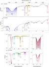 |
Fig. 1 Full NIRSpec and MIRI spectra for EDJ183-b and Per-emb35. The ice absorption features are shaded in color. The bottom panels show zoomed-in sections of the spectra. |
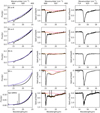 |
Fig. 2 Continuum and silicate subtraction for the 12CO2 bending mode in the 15 µm region. The left panel shows the fitting of the continuum (purple line). The middle panel shows the two Gaussian profiles (red and pink lines) and the combined final fit (orange line), which simulates the silicate absorption feature at 18 µm. The third panel shows the subtracted spectra after the silicate band was removed. The continuum subtraction for the remaining sources can be found in Appendix B.2.2. |
2.4 Column densities
The column densities for the vibrational modes were derived using
 (2)
(2)
where τv is the integrated absorbance under the absorption feature, and A is the corresponding band strength of the vibrational mode.
For the band strengths, we used the values determined by Gerakines et al. (1995) and Gerakines et al. (2005) and corrected by Bouilloud et al. (2015). All band strengths used in this work are listed in Table 1 and are further discussed along with the error analysis on the column densities in Appendix A. The column densities derived in this work can be multiplied by the correction factors given in Table 1 to compare them with the values derived using the band strengths reported in Gerakines et al. (1995) and Gerakines et al. (1995). We note that the recent band strengths Gerakines & Hudson (2015) derived for amorphous CO2 are similar to the corrected values we used in this work. The change in the band strength due to the ice mixture and the temperature are accounted for in the error analysis. Last, the 12C/13C ratios were determined for the bands as a whole and not for the individual components.
Band strengths of CO2 and CO ice.
Column densities and isotope ratios derived for 12CO2 and 13CO2 ice.
3 Analysis
We determined the column densities and derived the carbon isotope ratio for the 12CO2 v1 + v2 combination mode (2.70 µm), the 12CO2 v3 stretching mode (4.27 µm), the 13CO2 v3 stretching mode (4.39 µm), the 12CO2 v2 bending mode (15.2 µm), the 12CO 2-0 overtone mode (2.35 µm), the 12CO 1-0 stretching mode (4.67 µm), and the 13CO 1-0 stretching mode (4.78 µm). We also detected the 12CO2 2v1 + v2 combination mode (2.77 µm) in a number of sources. The list of sources, their luminosities, distances, and the column densities for each individual vibrational mode are presented in Tables 2 and 3 for CO2 and CO, respectively.
3.1 CO2
The 2.70, 4.27 and 15.2 µm vibrational modes of 12CO2 were collectively detected in a number of sources. For these sources, we derived the 12CO2/13CO2 ratios and found values that agree within the reported error bars (Table 2). The largest source of uncertainty in the derived ratios stems from the error on the band strengths, the observational errors are negligible in contrast (~3%). For the error on the band strengths, we accounted for the change in the band strength due to the temperature and due to the ice mixture, more specifically, a water-rich ice mixture, because it is known that ~50% of the CO2 resides in a water-rich matrix (Pontoppidan et al. 2003; Brunken et al. 2024).
The CO2-H2O binary ices affect each vibrational mode of CO2 differently. The band strengths of the 2.70, 4.27, and 4.39 µm bands, for instance, decrease relative to the band strength of pure CO2 when CO2 is mixed with water. This subsequently results in higher 12CO2 and 13CO2 column densities (Gerakines et al. 1995). The band strength of the 15.2 µm band, in contrast, increases by a significant amount relative to the band strength of pure CO2, resulting in lower 12CO2 column densities. This therefore introduces a systematic error when the ratios from the different vibrational modes are calculated because ratios derived from the 15.2 µm band are lower in general than ratios derived from the other 12CO2 vibrational modes when a band strength for a CO2-H2O mixture is used. We used the band strength of pure CO2 and accounted for this systematic error in the error analysis. For a detailed analysis of these uncertainties, we refer to Appendix A.
3.1.1 The 12CO2 2.70 and 2.77 µm combination modes
The assignment of the 2.70 µm band has been the topic of multiple studies. Keane et al. (2001), for instance, first fit this feature with laboratory spectra of CO-H2O (100:1) ices, but later assigned this feature to CO2 because the fraction of CO in the binary CO-H2O ices was inconsistent with the amount of CO present in the other bands. The band has also been assigned to the OH-dangling mode of porous water ice because water has multiple weak features in this spectral region (Noble et al. 2024). In our sample, we detect this 2.70 µm feature in 9 out of 17 sources on the short-wavelength side of the OH-dangling mode, situated at 2.75 µm (Figure 3), and we assigned this band to the combination mode of CO2 for the following reasons.
First, we fit several spectra of pure CO2 ice and CO2 in mixtures with CO, H2O, and CH3OH (Pontoppidan et al. 2008), and we found an absorption feature at 2.70 µm for every mixture containing CO2, as illustrated in Figure 4. The dangling modes of pure porous water ice and water ice mixed with other ice species do not sufficiently fit the observed profile of this feature. Additionally, we detect the OH-dangling mode of water ice interacting with other species at 2.75 µm in every source in which the combination mode is present, except for Per-emb35, where it disappears (Figure 3). This source shows clear signs of thermal processing with double-peak profiles at 4.39 µm (13CO2) (Brunken et al. 2024) and 15.2 µm (12CO2) (Pontoppidan et al. 2008) (Figures B. 9, B. 10, B. 4 and B. 5).
OH-dangling modes originate from non-H bonded OH-groups of cold amorphous water ice that is either porous or in mixtures with other species that disrupt the H-bonding network (Keane et al. 2001; Noble et al. 2024), and experimental studies have shown that the strength of these bands decreases with increasing temperature (Isokoski et al. 2014). This is because the elevated temperatures cause the molecules to restructure and form bonds, which in turn will lead to a decrease in the number of free OH-groups and the strength of the OH-dangling modes. A gradual decrease of OH trapping sites due to ice heating was also shown in experimental results by Sandford & Allamandola (1988), where the H2O-CO shoulder that was observed at 4.64 µm disappeared when the amorphous H2O ice structure was annealed. Since the 4.39 and 15.2 µm bands of Per-emb35 show clear signs of thermal processing, the absence of the 2.75 µm band in this source is therefore likely the result of the amorphous porous water structure disappearing due to the elevated temperatures in the envelope.
If both the 2.70 and the 2.75 µm bands were indeed water OH-dangling modes, however, then the 2.70 µm feature should also disappear when the ices undergo thermal processing. We instead observe a sharpening of the profile and the appearance of a sharp peak on the short-wavelength side of the band, which we successfully reproduced with the spectrum of pure CO2 and the alternative spectral decomposition for warm ices described in Brunken et al. (2024) (Figure 4). This behavior is similar to the behavior observed at 4.39 and 15.2 µm when pure CO2 ice begins to segregate from the ice matrix. This strongly indicates that the 2.70 µm feature therefore cannot primarily be the product of OH-dangling modes. We note that the 2.75 µm OH-dangling mode is detected in the extended sources Ser-S68N-N and Ser-SMM3 (Figure B. 12, where the ices are also processed, but this could be due to the fact that we might be tracing a fraction of cold-ice components in the extended envelopes of these sources.
Finally, while laboratory spectra have shown OH-dangling bonds at 2.70 µm for water ice with high porosity, we note that the method of depositing gas-phase water to form very porous water is inconsistent with the mechanism of interstellar ice formation through atom addition, which produces more compact ices. Therefore, we assigned the 2.70 µm feature to the combination mode of CO2 and quantified the column density of 12CO2 from this band (Figure 5). The ratios extracted from this band are presented in Table 2.
We note that the column densities we derived from the 2.70 µm band are consistent with the column densities extracted from the other two 12CO2 vibrational modes in both our cold and heated sources, except for Ser-SMM3. This is further evidence that the majority of this band is indeed for the most part the 12CO2 combination mode.
We also observed the 2v1 + v2 combination mode at 2.77 µm in Per-emb35 and Ser-SMM3 (Figure B. 12). The band strength of this feature is lower by a factor ~3 than that of the 2.70 µm, however, and it is also highly susceptible to changes in the temperature, even more so than its counterpart at 2.70 µm. Because of these high uncertainties, we refrained from quantifying carbon isotope ratios from this weak feature.
Column densities and isotope ratios derived for 12CO and 13CO ice.
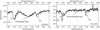 |
Fig. 3 12CO2 combination mode (2.70 µm) and water OH-dangling mode (2.75 µm) for the sources EDJ183-a (not heated) and Per-emb35 (heated). The feature at 2.75 µm is not detected in Per-emb35, while the 2.70 µm feature is detected in both sources. |
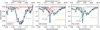 |
Fig. 4 Profile decomposition of the 12CO2 2.70 µm combination mode using selected laboratory spectra based on the analysis performed in Brunken et al. (2024). In the left and middle panel, the black line shows the observed spectrum, and the blue line shows the linear combination of all the five different components at low temperature. The yellow line corresponds to the CO2:CH3OH (10 K) component. The pink line shows the contribution of the broad CO2:H2O (10 K) component. The purple line corresponds to the diluted CO2:CO (25 K) component, and the orange line shows the contribution of CO2 and CO mixed in an equal ratio (15 K). Finally, the dark red line corresponds to the pure CO2 (80 K) component. In the right panel, the black line shows the observed spectrum, and the blue line shows the linear combination of all the three different components at high temperatures. The green line corresponds to the hot CO2:CH3OH (105 K) component. The gray line shows the contribution of the hot CO2:H2O (160 K) component. Finally, the dark red line corresponds to the pure CO2 (80 K) component. All laboratory spectra are taken from Ehrenfreund et al. (1997, 1999); van Broekhuizen et al. (2006) and are publicly available in the Leiden Ice Database (LIDA) (Rocha et al. 2022). Further details of the laboratory spectra can be found in Brunken et al. (2024). |
3.1.2 The 12CO2 4.27 µm stretching mode
In Figure 6 we present the 4.27 µm stretching mode for 6 out of 17 sources. While this band is detected in the remaining sources, they are all highly saturated (τ > 5 ). As a test for using the 4.27 µm band for saturated sources, we fit the laboratory spectrum of CO2:H2O 1:10 at 10 K (Ehrenfreund et al. 1999) to the wings of the 4.27 µm band in Per-emb35 using the 15.2 µm bending mode as an anchor.
Overall, the band profiles of the selected six sources appear to be very similar, and only the slope of the short-wavelength wing varied depending on the source. Additionally, the strength of the scattering feature on the short-wavelength wing differed per source. The column densities derived from this band agree well with the column densities derived from the 2.70 µm combination mode for each source.
For the fitted band of Per-emb35, we find a 12CO2/13CO2 ratio of ~80 ± 21 (Figure B. 14). This value is consistent within the reported error bars with the ratios derived from the other two vibrational modes in this same source. Due to the ambiguity of the true band profiles and optical depths of these saturated bands, however, we omitted the band of these sources from this study.
3.1.3 The 12CO2 15.2 µm bending mode
The 15.2 µm bending mode is detected in all 17 sources, each showing distinctive band profiles (Figures 2, B.9, B.10, and B.11). The sources with a double-peak profile are most notable because this is a telltale sign of ice heating (Ehrenfreund et al. 1998; Pontoppidan et al. 2008).
In Section 2.3.3 we discussed the continuum subtraction method and the extended wing-profile after subtracting the silicate model. We investigated the effect of this extended wing in comparison to the wing profile of Pontoppidan et al. (2008), which extends to ~16 µm instead of ~18 µm, and found a difference in column density of ~9%, which is negligible compared to the uncertainties of the band strengths (see also Appendix A). The column densities derived from the bending mode are presented in Table 2.
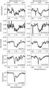 |
Fig. 5 Overview of the 12CO2 combination modes. |
3.1.4 The 13CO2 4.39 µm stretching mode
13CO2 column densities were derived from the 4.39 µm band for all 17 sources (Table 2). Consistent with the 15.2 µm band, we observe a double-peak profile at 4.39 µm for every source with a split peak at 15.2 µm. One hindrance is the CO line forest, which bleeds into the 13CO2 band of several sources in this sample, potentially causing a slight underestimation of the 13CO2 column densities. We briefly investigated the effect of the gaseous CO lines in EDJ183-b by fitting a Gaussian profile to the bottom of the 13CO2 band and quantifying the column density from this curve. We find that the 12CO2/13CO2 ratio decreases by 35% when the integrated optical depth is determined from the Gaussian curve instead of directly from the band. In Figure B.7 we show the Gaussian curves that were ultimately used to determine the integrated optical depths for the 13CO2 bands that are most affected by the gaseous CO lines. For the sources where the 13CO2 features were well isolated from the line forest, the integrated optical depths were directly determined from the ice bands.
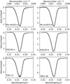 |
Fig. 6 Overview of the 12CO2 4.27 µm stretching mode. The features are shown for sources for which the band is not saturated. |
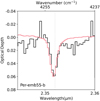 |
Fig. 7 Source Per-emb55b and the 2.35 µm feature. The laboratory spectrum of pure CO is plotted over the v = 2−0 absorption feature (pink). |
3.1.5 12CO2/13CO2
In Table 2 we compare the column densities and ratios derived from the different CO2 ice features. For the sources in which the 2.70 µm combination mode, the 4.27 µm stretching mode, and the 15.2 µm bending mode are detected, we find consistent ratios, except for TMC1-W, where the ratio derived from the 4.27 µm stretching mode is ~25% lower than the values extracted from both the 2.70 and the 15.2 µm bands. This deviation still lies within our reported error bars, however. We also find a discrepancy of ~50% between the ratio derived from the 2.70 and the 15.2 µm bands in Ser-SMM3.
For the 2.70 µm band, the 4.27 µm band, and the 15.2 µm band, we find mean 12CO2/13CO2 ratios of 85 ± 23, 76 ± 12, and 97 ± 17, respectively. These are similar to the median values we derived from these vibrational modes (see also Section 4.1). We note that the variation in ratios derived for the different sources and the uncertainty margin on the mean ratios could in fact be due to genuine differences that reflect the different chemical conditions of these systems.
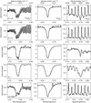 |
Fig. 8 Overview of the 13CO2 (left), 12CO (middle), and 13CO (right) stretching modes in the 4 µm region. The 12CO gas-phase lines are shown superimposed in several sources. |
3.2 CO
3.2.1 The 12CO 2.35 µm overtone mode
We detected a weak absorption feature at 2.35 µm above 3σ level for 6 out of the 17 sources (TMC1-E, TMC1-W, Per-emb55-b, EJD183-a, EDJ183-b, and Ser-S68N-N). In previous experimental work, this band was assigned to the ν = 2-0 overtone mode of CO, which peaks at this wavelength in the near-infrared (Fink & Sill 1982; Gerakines et al. 2005). We used experimental data of pure CO to analyze the band profiles of these absorption features and found that the peak position of all sources except that of Per-emb55-b were significantly redshifted (Figure 7).
The sources in which the 2.35 µm features are redshifted also display strong gas-phase CO overtone photospheric absorption lines that peak in the 2 µm spectral region. These gaseous CO overtone modes originate from the central protostellar embryo and appear in absorption due to the strong thermal gradient of the gas surrounding the protostar (Le Gouellec et al. 2024). These gas-phase absorption lines include the ν = 4-2 line at 2.3525 µm, which overlaps the 2.35 µm CO ice absorption band and causes the redshifted ice bands we observed in most of these sources.
In order to disentangle and subtract the gaseous CO overtone modes, the 2 µm hot dust emission was first modeled with a blackbody emission. The photosphere was modeled using the BT-Settl grid of photospheric models (Allard et al. 2012). The Starfish modeling framework from Czekala et al. (2015) was used (see also Figure B.15). Further details of these modeling procedures are presented in Le Gouellec et al. (in prep.). The findings show that the models converged well in TMC1-E, TMC1-W, EDJ183-a, EDJ183-b, and Ser-S68N-N, and after subtraction, no residual ice features were observed in these sources. A faint photosphere is detected in Per-emb55-a, and a weak absorption feature is visible at 2.35 µm. This feature, however, is faint and hard to separate from the noise spikes in the spectrum. In Per-emb55-b, no photosphere was detected, and we can conclude that the 2.35 µm feature is indeed the CO overtone ice absorption band.
Because of the gas contamination, we discarded the other five sources in which these gas signatures were observed and only extracted the 12CO column density from the band observed in Per-emb55-b (Figure 7). The column density we derived from this band is lower by a factor ~1.6 than the column density derived from the 4.67 µm band in this same source. One possible explanation for the discrepancy between these two vibrational modes is the band strength of this relatively weak absorption feature.
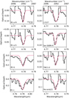 |
Fig. 9 Zoom-in of the 13CO absorption features. The Gaussian curves (pink) fit to the bands illustrate the bounds we used to determine the integrated optical depths. |
3.2.2 The 12CO 4.67 µm stretching mode
The bands of the 12CO 4.67 µm symmetric stretching mode are presented in Figures 8, B.4, B.5, and B.6, and the column densities are listed in Table 3. We find variations of more than an order of magnitude between the different sources and ascribe this to the volatility of CO. Because of its lower desorption temperature, CO ice is highly sensitive to the temperature structure of the protostellar envelope, which in turn can significantly impact the CO ice budget and cause variations depending on the source.
3.2.3 The 13CO 4.78 µm stretching mode
The 13CO 4.78 µm stretching mode is observed in 14 out of 17 sources, only 2 of which are well isolated from the CO gasphase rotation-vibrational lines (B1-b and B1-c). The strong line forest that dominates most of the sources in this sample poses a challenge to the study of this weak feature because the actual shape and optical depth of this band are likely affected by the gas lines. We briefly investigated the effect of the emission lines by fitting Gaussian profiles and subtracting the two gaseous CO lines closest to the bands, and we find that the 13CO column density increases by a factor 1.4 compared to the nonsubtracted band. This is still within our reported uncertainties. We note, however, that the gas-subtracted 13CO ice bands are significantly broader than the nonsubtracted bands and are also much broader than the band of the laboratory spectrum of pure CO, which could be the main contributor of this band (Boogert et al. 2002a; Pontoppidan et al. 2003). On the other hand, a broad band profile is possible when the 13CO ice resides in a polar CH3OH-rich ice matrix (Penteado et al. 2015). A careful modeling and removal of the gaseous CO lines is needed in order to properly isolate the ice feature and quantify the 13CO ice column density. This CO gas modeling is beyond the scope of this paper, however. In Figures 9 and B.8, we show the Gaussian curves that were fit to the 13CO features in order to determine the integrated optical depths.
3.2.4 12CO/13CO
The carbon isotope ratios derived from the CO ice absorption bands are presented in Table 3. In general, we find high 12CO/13CO ratios. The sources B1-a-S, Per-emb22, Per-emb33, Ser-S68N-N, and Per-emb27 in particular have very high ratios, all of which also have very weak 13CO ice absorption features. Moreover, the 13CO ice bands of some of these sources are buried in the gas line forest, which could be the reason for some of these extreme ratios. We derived a sub-ISM ratio for source B1-c, but we note that the spectrum of this source was taken at medium resolution unlike the other sources in this sample. Consequently, the narrow 13CO band might not be fully resolved. Additionally, the gaseous CO lines in this source are in absorption and could be blended with the unresolved ice feature further contributing to its width.
Finally, we derived a 12CO/13C ratio of 96 ± 14 from 2.35 µm overtone mode in Per-emb55-a, which is lower by a factor ~1.6 than the ratio of 152 ± 23 derived in this same source from the 4.67 µm band. For the 4.67 µm band, we find a mean 12CO/13CO ratio of 165 ± 52 for the sample as whole when we exclude the three extreme outliers Per-emb22, Per-emb33, and Per-emb27. Due to the fluctuating values derived from the CO vibrational modes, we recommend referring to the ratios derived from the CO2 vibrational modes rather than the CO ice bands.
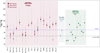 |
Fig. 10 Solid 12C/13C for various astronomical environments. The filled red, gray, and white stars represent the ratios derived from the 12CO2 15.2, 4.27, and 2.70 µm bands, respectively. We also include molecular clouds (Ice Age) (McClure et al. 2023) and a massive YSO (Infrared Space Observatory). (Boogert et al. 2000). The dashed purple line shows the solar abundance, and the dot-dashed gray line shows the local ISM ratio (Boogert et al. 2000). The small solid error bars of the JOYS+ data points illustrate when the band strengths were excluded from the error analysis. The faint and generally larger error bars of the JOYS+ data points illustrate the uncertainty, including the error on the band strength. Further details of the error analysis can be found in Appendix A. |
3.3 Limitations and future work
As shown in the previous sections, we examined the carbon isotope ratios for multiple CO and CO2 vibrational modes for a large sample of low-mass sources. We found consistent values for the most part, especially between the ratios derived from the CO2 ice bands. One source of uncertainty are the band strengths, especially for the weaker 12CO overtone mode. The 4.40– 4.5 µm spectral region is also heavily dominated by gaseous CO rotation-vibrational lines, which poses a challenge when quantifying 13CO column densities from the absorption feature at 4.78 µm. Therefore, a careful modeling and subtraction of these gas lines is needed to properly isolate it in the 13CO ice features and determine 13CO column densities. Alternatively, spectral extractions at locations where the gas-phase lines are weak or absent could also aid in the analysis of the 13CO ice features. Finally, future work should also focus on finding similarities or variations between close binaries, and a spatial ice mapping should be performed since this feat is now possible with the JWST.
4 Discussion
The carbon isotope ratio is a crucial link between the evolutionary phases of star and planet formation because of its sensitivity to the chemical and physical conditions that reign during each stage. In the following section, we examine how the results presented in this work relate to the trends observed in different astronomical environments both in the solid state and in the gas phase.
4.1 Protostars: Solid state
4.1.1 CO2
The 12C/13C ratios we derived from solid CO2 for the JOYS+ sample are presented in Figure 10, along with the isotope ratios derived in the solid state for the Infrared Space Observatory (ISO) study of young stellar objects (Boogert et al. 2000) and two highly extincted lines of sight (McClure et al. 2023) in the Cha I molecular cloud. We note that although previous studies used the uncorrected Gerakines et al. (1995) band strengths, the corrections do no affect the relative band strengths, and consequently, do not affect the 12C/13C ratios. For this reason, the ratios determined in these previous studies can be directly compared to the ratios derived in this work. The light error bars of the JOYS+ data points illustrate the uncertainties, including the error on the band strengths, and the solid error bars illustrate the uncertainties, excluding the error on the band strengths. The errors in the band strengths account for the change in the band strength due to the temperature and ice mixture. The small error bars when the uncertainty on the band strengths are excluded demonstrate the great capabilities of the JWST and the high quality of these data. Previous studies generally did not include a detailed analysis of the uncertainty in the band strengths in their error bars.
The results show that the ratios obtained from the 15.2 µm bands are clustered slightly above the ISM ratio of 68 (Boogert et al. 2000; Milam et al. 2005). This suggests that the ices in our sources are slightly deficient in 13C in comparison to the local ISM. When we detect all three 12CO2 vibrational modes, we find consistent column densities and ratios (Figure 10). This is further evidence that the 2.70 µm feature primarily consists of the 12CO2 combination mode. These consistent values also show that the 4.27 µm stretching mode can be used to determine 12CO2 column densities when the other 12CO2 bands are not available and when the stretching mode is not saturated.
When compared to other solid-state studies of carbon isotope ratios, the 12CO2/13CO2 ratios measured in our sample are fairly consistent with the those found in the ISO-SWS high-mass sources by Boogert et al. (2000) (ranging 52–113). Similar to the JOYS+ sources, the authors reported values that are scattered around the local ISM ratio, but they also reported sub-ISM values as low as 52. These sub-ISM ratios still agree with our values within the reported error bars. Figure 11 illustrates the distribution of the 12CO2/13CO2 ratio for the JOYS+ sample and the ISO high-mass sources (Boogert et al. 2000). While a large fraction of the ISO MYSOs also displays elevated ratios with respect to the ISM standard, the ratios of the JOYS+ protostars are in general higher, with median values of 81, 75, and 100 for the 2.70 µm combination mode, the 4.27 µm stretching mode, and the 15.2 µm bending mode, respectively. These are similar to the mean values of 85 ± 23, 76 ± 12, and 97 ± 17 derived for these bands, respectively. The agreement between the ratios derived from the different CO2 vibrational modes of the JOYS+ protostars again shows the great capability of the JWST to accurately probe different lines of sight and observe the weak ice features in the 2 µm region, the generally saturated strong stretching mode at 4.27 µm, and the bending mode at 15.2 µm.
Our values are also consistent if slightly higher than the values reported in McClure et al. (2023) for the two lines of sight in the Cha I molecular cloud (12CO2/13CO2 ~ 69–87). We note, however, that the 12CO2 column densities derived for Cha I were extracted from the 4.27 µm bands, which are saturated in both lines of sight. Consequently, the 12CO2 column density could be somewhat underestimated in these sources. Furthermore, the uncertainties reported in McClure et al. (2023) did not include errors on the band strengths. Nonetheless, the consistency between the ratios derived from the protostellar stage and the dense-cloud stage paint the harmonious picture that the CO2 was likely inherited from its parent molecular cloud.
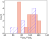 |
Fig. 11 Distribution of the 12CO2/13CO2 isotope ratio. The filled orange bars show the distribution of the carbon isotope ratios determined for the JOYS+ sample. These ratios were extracted from the 15.2 µm bending mode. The striped purple bars show the distribution of the carbon isotope ratio derived for the ISO high-mass sources (Boogert et al. 2000). |
4.1.2 CO
The 12CO/13CO ratios derived from solid CO for the JOYS+ sample are shown in Figure 12, along with the isotope ratios derived from various studies both in the gas and solid state. Similar to CO2, the corrections on the CO band strengths (Gerakines et al. 1995) have no effect on the 12C/13C ratio and values derived in previous solid-state studies can therefore be directly compared to the findings in this work. Overall, our results show that the isotope ratios obtained from the CO 4.67 µm stretching mode are considerably higher than the local ISM value. The ratios are also higher than the ratios previously derived for one MYSO (Boogert et al. 2002a) and one LYSO (Pontoppidan et al. 2003), both of which are very close to the ISM standard. This discrepancy likely arises because our 13CO column density is underestimated due to the weak 13CO ice absorption feature and the strong CO gas lineforest that dominates this spectral region. This is particularly the case for the three extreme outliers Per-emb22, Per-emb33, and Per-emb27 (shown only in Table 3), both of which exhibit strong gas-phase lines and weak 13CO ice bands (Figure B.5).
The ratio derived from the 2.35 µm feature in Per-emb55-b is also higher than the local ISM standard. When compared to the ratios derived in molecular clouds, however, our values are consistent with those found by McClure et al. (2023), who also reported super-ISM 12CO/13CO ratios (99–184) (Figure 12).
4.2 CO versus CO2 isotope ratios
The ratios derived from CO and CO2 from the JOYS+ sample are presented in Figure 12, along with gas-phase and solid-state ratios derived from various studies. Normally, the carbon isotope ratio of solid CO and CO2 is expected to be similar because the formation route of CO2 is tied to that of CO through the equation (3) (Ioppolo et al. 2011)
 (3)
(3)
In the ices of our sources, however, the 12CO/13CO ratios are higher in general than the 12CO2/13CO2 ratios derived from the 2.70, 4.27, and 15.2 µm bands, although they still agree within the error bars for a number of our sources. As noted in Section 4.1.2, a reason for this deviation could be that the CO ratios are less accurate because the 13CO ice feature is weak. Overall, we consider the CO2 -derived isotope ratios to be more reliable given the multiple methods we used to quantify this ratio.
4.3 Protostars: Gas phase
In the gas-phase, Smith et al. (2015) reported significant 12CO/13CO variability for several YSOs, with an overall trend of elevated ratios with respect to the local ISM standard (Figure 12). One possible scenario they proposed is gas-ice partitioning (Section 4.4.3), with an additional mechanism for removing 13CO from the solid state through the formation of larger complex organic molecules (COMs) from 13C-rich CO ices. Consequently, the COMs will be enriched 13C and exhibit low carbon isotope ratios, such as the sub-ISM values found in COMs by Jørgensen et al. (2016, 2018). We note, however, that the gasphase values reported by Smith et al. (2015) are similar to those derived in this study, which suggests that the ices might have sublimated from the grains, delivering the carbon isotope ratio to the gas during the pre-stellar stage.
The quantifying of gas-phase and solid-state isotope ratios in the same source was in fact proposed by Charnley et al. (2004) as a way of tracing the origin of organic material. Therefore, observations of gas-phase CO isotopologs for the JOYS+ protostars will be crucial for enabling this method of posterior isotopic labeling and linking the solid-state chemistry with the gas-phase chemistry in these systems. In the following section, we study the different mechanisms that can affect the carbon isotope ratio in both the solid and gas phase in the early stages of star and planet formation.
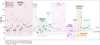 |
Fig. 12 12C/13C for various astronomical environments. The filled red, gray, and white stars represent the ratios derived from the 12CO2 15.2, 4.27, and 2.70 µm bands, respectively. The closed and open yellow stars represent the ratios derived from the 12CO 4.67 and 2.35 µm bands, respectively. The error bars on the JOYS+ data points include the error on the band strengths, which is the main contributor to these uncertainties. The ratios were taken from the following works: Ice age (McClure et al. 2023), (Boogert et al. 2000), KECK-NIRSpec (Boogert et al. 2002a), VLT (Pontoppidan et al. 2003), VLT-CRIRES (Smith et al. 2015), PILS (Jørgensen et al. 2016, 2018), Disks (Yoshida et al. 2022; Bergin et al. 2024), Exo-planets (Line et al. 2021; Zhang et al. 2021a,b; Gandhi et al. 2023; de Regt et al. 2024), Comets (Bockelée-Morvan et al. 2015; Hässig et al. 2017). The dashed purple line shows the solar abundance, and the dot-dashed gray line shows the local ISM ratio (Boogert et al. 2000). Further details of the error analysis can be found in Appendix A. |
4.4 Fractionation processes
4.4.1 Isotope-exchange reactions
Isotope-exchange reactions are exothermic reactions that are efficient at low temperatures and that prompt preferential incorporation of 13C+ in CO (Equation (4)) (Watson 1976; Langer et al. 1984; Langer & Penzias 1993). As a result, molecular 13CO is enhanced with respect to 12CO in the gas phase, and this low 12CO/13CO ratio is subsequently conveyed to the solid state upon CO freeze-out. 12C+, in contrast, is enhanced in the gas phase, leading to high 12C+/13C+ gas-phase ratios.
 (4)
(4)
4.4.2 Selective photodissociation
Selective photodissociation of 13CO is a destruction mechanism that occurs because self-shielding of the less abundant 13CO takes place at higher extinctions in comparison to 12CO (van Dishoeck & Black 1988; Visser et al. 2009). This leaves a large portion of the 13CO gas vulnerable to ultraviolet radiation. As a result, 13CO is destroyed, which increases the gaseous 12CO/13CO ratio and decreases the 12C+/13C+ ratios as the molecules dissociate and the gas is enriched with 13C+ and O atoms. This counters the effect of isotope selective photodissociation (Section 4.4.1). This high molecular 12CO/13CO ratio translates into the solid state upon CO freeze-out, producing ices that are depleted in 13C. Although we expect that under dark cloud conditions, most of the radiation is attenuated by the high-density environment, thus limiting the effect of selective photodissociation, studies by Furuya & Aikawa (2018) have shown that turbulence can transfer selective photodissociated material to the dark inner regions of clouds.
4.4.3 Gas-ice partitioning
A third mass-dependent mechanism was proposed by Smith et al. (2015), who reported that a small difference in the binding energies of 12CO and the slightly heavier 13CO (∆Ebind~10 K) resulted in 12CO desorbing at a slightly lower temperature from the grains. Consequently, the 12CO/13CO in the gas phase is enhanced while the ices become enriched with 13CO, leading to low carbon isotope ratios in the solid state. It is worth noting, however, that gas-ice partitioning is only effective during a very narrow temperature window (Smith et al. 2015).
Of the mechanism discussed above, selective photodissociation could be causing the 13C deficiency that is observed in this sample, although its efficiency under these conditions is open to question.
4.5 Evolution of the 12C/13C ratio
As the stellar system matures, different process begin to dominate. They slowly erode the initial carbon isotope ratio of the pristine material. In the following sections, we discuss the evolution of the carbon isotope ratio during the later epochs of star formation.
4.5.1 Protoplanetary disks
Studies of carbon isotope ratios in disks revealed that at this stage, the conditions in the system are irrevocably changed and that the initial carbon isotope imprint can be effectively erased in certain regions of the disk. Yoshida et al. (2022) and Bergin et al. (2024), for instance, found a dichotomy in the TW Hya disk, where two different carbon isotope ratios were measured for CO and C2H (21 ± 5 and 65 ± 20, respectively). In the same disk, Hily-Blant et al. (2019) found a ratio of 86 ± 4 from HCN rotational lines.
The variability of the carbon isotope ratio in protoplane- tary disks arises because the ratio is contingent on the location in which the molecules were formed. This is because different processes dominate in different regions of the disk. Photodissociation, for instance, plays a significant role in the upper layers of the disk, where the high ratio derived from C2H is found, while isotope-exchange reactions are more efficient in the midplane and at larger radii, where the temperatures are low and where the low value for CO is measured (Willacy & Woods 2009; Visser et al. 2018; Bergin et al. 2024).
4.5.2 Exoplanets
The large variability in the carbon isotope abundance is also observed in the atmospheres of exoplanets, where the formation mechanism of the planet plays a crucial role in its carbon isotope reservoir. Recent observational efforts by Zhang et al. (2021a); Line et al. (2021); Gandhi et al. (2023), for instance, revealed a significant enrichment of 13CO in the atmospheres of hot Jupiters (31±17, 10.2–42.6 with a confidence of 68%, and 62 ±2, respectively). This 13C enrichment is likely because the planet was formed beyond the CO snowline and accreted most of its material from 13C-rich ices. These 13C-rich ices are likely the result of fractionation processes such as isotope-exchange reactions and possibly gas-ice partitioning, which must have occurred after the protostellar stage.
Zhang et al. (2021b); de Regt et al. (2024), in contrast, measured very high 12C/13C ratios (97 ± 15 and 184 ± 61, respectively) for brown dwarfs, which indicates a formation route similar to that of stars, where the object forms from cloud fragmentation and gravitational collapse and inherits most of its gaseous material from a parent cloud that is also deficient in 13C and 13C-ices, as we found here. This shows that the carbon isotope ratio is a potentially powerful tool for tracing the formation pathways of extrasolar planets.
4.5.3 Comets and meteorites
The chemical complexity of the infant planetary system is at last fossilized in the remains of its building blocks, the comets. Observations of C2, CN, and HCN in numerous comets, for instance, showed that the carbon isotope ratios of Solar System objects are all similar to the solar abundance (~89), with little variation between the ratios (Bockelée-Morvan et al. 2015). Similarly, Alexander et al. (2007) reported ratios consistent with the solar abundance from a large study of 75 chondrites. Finally, Hässig et al. (2017) also derived a ratio of 84 ± 4 from CO2 measurements in the coma of comet 67P/Churyumov-Gerasimenko. It is worth noting that the carbon isotope ratio found in comets and chondrites resembles the values derived in the protostel- lar stage. This could be an indication that while fractionation processes erode the initial carbon isotope imprint during the later stages, a fraction of the pristine material still survives this journey and is eventually incorporated into the planetary system.
5 Conclusions
We have analyzed JWST NIRSpec and MIRI data of 17 Class 0/1 low-mass protostars and determined the 12CO, 13CO 12CO2, and 13CO2 column densities and 12C/13C isotope ratios from the 12CO2 v1 + v2 and 2v1 + v2 combination modes (2.70 µm and 2.77 µm), the 12CO2 v3 stretching mode (4.27 µm), the 13CO2 v3 stretching mode (4.39 µm), the 12CO2 v2 bending mode (15.2 µm), the 12CO 2-0 overtone mode (2.35 µm), the 12CO 1-0 stretching mode (4.67 µm), and the 13CO 1-0 stretching mode (4.78 µm). The most significant finding is that the ratios are consistent if slightly higher than the local ISM value. These results show that the ices leave the protostellar stage with high 12C/13C ratios, after which a series of fractionation processes during the later stages could modify the initial isotope abundance.
The absorption feature observed at 2.70 µm in 9 out 17 sources is assigned to the combination mode of 12CO2. We also detect the 2.77 µm combination mode of 12CO2 in two sources.
We find consistent 12CO2/13CO2 ratios between the 4.27 µm, 15.2 µm, and the 2.70 µm bands. Our values are slightly elevated with respect to the standard ISM value, but they are consistent with carbon isotope ratios observed in other protostars and in dark molecular clouds. We observe variations in the 12CO2/13CO2 ratio from one source to the next, which might indicate genuine differences in the chemical complexity of their protostellar envelopes.
We report a detection of the 2.35 µm ν 2-0 12CO overtone mode in one source.
The 12CO/13CO ratios derived from the 4.67 µm band are higher than the local ISM ratio and the 12CO2/13CO2 ratios. The ratio derived from the overtone mode is lower by a factor ~1.6 than the ratio extracted from the 4.67 µm band in the same source.
Our findings show that fractionation processes begin to dominate after the protostellar stage. Future work should be focused on ice spatial mapping of close binary pairs and extended protostellar envelopes, and on obtaining observations of the gas-phase CO isotopologs of the JOYS+ sample in order to compare solid-state and gas-phase carbon isotope ratios.
Data availability
Appendices B and C are available on Zenodo.
Acknowledgements
Astrochemistry in Leiden is supported by the Netherlands Research School for Astronomy (NOVA), by funding from the European Research Council (ERC) under the European Union’s Horizon 2020 research and innovation programme (grant agreement No. 101019751 MOLDISK), and by the Dutch Research Council (NWO) grant 618.000.001. Support by the Danish National Research Foundation through the Center of Excellence “InterCat” (Grant agreement no.: DNRF150) is also acknowledged. This work is based on observations made with the NASA/ESA/CSA James Webb Space Telescope. The data were obtained from the Mikulski Archive for Space Telescopes at the Space Telescope Science Institute, which is operated by the Association of Universities for Research in Astronomy, Inc., under NASA contract NAS 5- 03127 for JWST. The following National and International Funding Agencies funded and supported the MIRI development: NASA; ESA; Belgian Science Policy Office (BELSPO); Centre Nationale d’Etudes Spatiales (CNES); Danish National Space Centre; Deutsches Zentrum fur Luft- und Raumfahrt (DLR); Enterprise Ireland; Ministerio De Economiá y Competividad; Netherlands Research School for Astronomy (NOVA); Netherlands Organisation for Scientific Research (NWO); Sci- ence and Technology Facilities Council; Swiss Space Office; Swedish National Space Agency; and UK Space Agency. N.B. thanks K. Pontoppidan for his contribution to the NIRSpec data reduction and helpful discussions. P.J.K. acknowledges support from the Science Foundation Ireland/Irish Research Council Pathway program under grant No. 21/PATH-S/9360. L.M. acknowledges the financial support of DAE and DST-SERB research grant (MTR/2021/000864) of the Government of India.
Appendix A Error analysis
The uncertainties on the derived isotope ratios are mostly sensitive to the uncertainties in the band strengths. Minor contributors are also the error on the placement of the continuum and the noise level. To ultimately set constraints on the ratios we must take all these factors into account when calculating column densities.
The ratio for the CO and CO2 bands are calculated as follows:
 (A.1)
(A.1)
where  and
and  are the column densities of 12CO2 and 13CO2 respectively,
  and
and  are the integrated optical depths and
  and
and  are the band strengths of the 12CO2 and 13CO2 vibrational modes respectively.
From equation A.1, the uncertainty on the ratio is determined following the error propagation rules:
 (A.2)
(A.2)
where  and
and  are the uncertainties on the integrated optical depth for 12CO2 and 13CO2 respectively.
The uncertainty on the integrated optical depth is influenced by the uncertainty in the placement of the continuum and the noise level and is determined as follows:
 (A.3)
(A.3)
where σint.OD,cont is the uncertainty due to the placement of the continuum, int.OD,cont is the integrated optical depth with the continuum of choice, σnoise is the uncertainty due to the noise level and int.OD,noise is the integrated optical depth. These parameters are calculated in a similar manner for 13CO2.
A.1 Continuum placement
We determine the uncertainty on the placement of the continuum by fitting the bands with two different baselines and using the difference in integrated optical depth as the uncertainty.
A.2 Noise level
The uncertainty due to the noise level is determined by calculating the rms in line free regions on flux scale (σf, λ) and propagating this to optical depth scale (σƒ,τ) following the error propagation rules for logarithms:
 (A.4)
(A.4)
since the observed fluxes  are converted to optical depth scale following equation (A.5),
 (A.5)
(A.5)
where  is the flux of the continuum.
We take Fcont,λ as constant since the uncertainty for that parameter is determined separately.
We use σƒ,λ to generate a noise level following a normal distribution and resample the spectrum with this added noise. We calculate the integrated optical depth for these resampled spectra which produces a sampling distribution that we can fit a Gaussian curve to (Figure A.1). From the Gaussian curve we can extract σnoise and int.OD,noise. This approach is similar to bootstrapping statistics and the contribution of this uncertainty is very small.
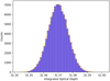 |
Fig. A.1 Sampling distrubition of the integrated optical depth. The dashed shows the Gaussian curve fitted to the distribution from which we extract σnoise and int.OD,noise. |
A.3 Band strengths
The column density for each vibrational mode is determined as follows:
 (A.6)
(A.6)
where A is the band strengths for of the corresponding vibrational mode.
As mentioned, we use the Gerakines et al. (1995) and Gerakines et al. (2005) band strength corrected by Bouilloud et al. (2015) to calculate the column densities.
The contributing factors to the uncertainty on the band strength for  are the placement of the continua (since we are considering relative errors), the uncertainty due to changes in the temperature of the ice and the uncertainty due to the ice mixtures. Since we know that the water component is a has a large contribution to the total band we took the uncertainties determined for the ice mixture CO2:H2O 1:24 binary ices. All values used in this work are reported in Table 1.
For the error due to the continuum we assume an uncertainty of 5% since Gerakines et al. (1995) only reports uncertainties >5% and no uncertainty is reported for this band strength. The uncertainty due to change in temperature is ~ 10% (Gerakines et al. 1995). Uncertainties for  are reported in Gerakines et al. (1995).
Taking all these assumption into consideration we determine the uncertainties on the band strengths as follows:
 (A.7)
(A.7)
The uncertainties on the CO column densities are determined in a similar manner with following exceptions:
We do not have mixture component for the error on the band strengths since we expect CO to be mainly in its pure form Pontoppidan et al. (2003)
We do not have a temperature component for the error on the band strengths since CO disorbs above 40 K.
We take a 10% error on the band strength for both the 12CO bands and the 13CO to the placement of the continuum in laboratory spectra.
The uncertainty on the integrated optical depth of the 13CO ice feature between gas-subtracted spectra and non-gas subtracted spectra is ~ 50 %. This is not included in the error bars of the figures.
References
- Alexander, C. M. O. D., Fogel, M., Yabuta, H., & Cody, G. D. 2007, Geochim. Cosmochim. Acta, 71, 4380 [NASA ADS] [CrossRef] [Google Scholar]
- Allard, F., Homeier, D., & Freytag, B. 2012, Phil. Trans. R. Soc. London Ser. A, 370, 2765 [Google Scholar]
- Argyriou, I., Glasse, A., Law, D. R., et al. 2023, A&A, 675, A111 [NASA ADS] [CrossRef] [EDP Sciences] [Google Scholar]
- Bergin, E. A., Melnick, G. J., Gerakines, P. A., Neufeld, D. A., & Whittet, D. C. B. 2005, ApJ, 627, L33 [NASA ADS] [CrossRef] [Google Scholar]
- Bergin, E. A., Bosman, A., Teague, R., et al. 2024, arXiv e-prints [arXiv:2403.09739] [Google Scholar]
- Beuther, H., van Dishoeck, E. F., Tychoniec, L., et al. 2023, A&A, 673, A121 [NASA ADS] [CrossRef] [EDP Sciences] [Google Scholar]
- Bockelée-Morvan, D., Calmonte, U., Charnley, S., et al. 2015, Space Sci. Rev., 197, 47 [Google Scholar]
- Böker, T., Arribas, S., Lützgendorf, N., et al. 2022, A&A, 661, A82 [NASA ADS] [CrossRef] [EDP Sciences] [Google Scholar]
- Boogert, A. C. A., Ehrenfreund, P., Gerakines, P. A., et al. 2000, A&A, 353, 349 [NASA ADS] [Google Scholar]
- Boogert, A. C. A., Blake, G. A., & Tielens, A. G. G. M. 2002a, ApJ, 577, 271 [NASA ADS] [CrossRef] [Google Scholar]
- Boogert, A. C. A., Hogerheijde, M. R., & Blake, G. A. 2002b, ApJ, 568, 761 [NASA ADS] [CrossRef] [Google Scholar]
- Boogert, A. C. A., Gerakines, P. A., & Whittet, D. C. B. 2015, ARA&A, 53, 541 [Google Scholar]
- Booth, A. S., Walsh, C., & Ilee, J. D. 2019, A&A, 629, A75 [NASA ADS] [CrossRef] [EDP Sciences] [Google Scholar]
- Booth, A. S., Leemker, M., van Dishoeck, E. F., et al. 2024, AJ, 167, 164 [NASA ADS] [CrossRef] [Google Scholar]
- Bouilloud, M., Fray, N., Bénilan, Y., et al. 2015, MNRAS, 451, 2145 [Google Scholar]
- Brunken, N. G. C., Rocha, W. R. M., van Dishoeck, E. F., et al. 2024, A&A, 685, A27 [NASA ADS] [CrossRef] [EDP Sciences] [Google Scholar]
- Bushouse, H., Eisenhamer, J., Dencheva, N., et al. 2024, https://doi.org/ 10.5281/zenodo.10870758 [Google Scholar]
- Caselli, P., & Ceccarelli, C. 2012, A&A Rev., 20, 56 [NASA ADS] [CrossRef] [Google Scholar]
- Charnley, S. B., Ehrenfreund, P., Millar, T. J., et al. 2004, MNRAS, 347, 157 [NASA ADS] [CrossRef] [Google Scholar]
- Christiaens, V., Samland, M., Gasman, D., Temmink, M., & Perotti, G. 2024, Astrophysics Source Code Library [record ascl:2403.007] [Google Scholar]
- Czekala, I., Andrews, S. M., Mandel, K. S., Hogg, D. W., & Green, G. M. 2015, ApJ, 812, 128 [NASA ADS] [CrossRef] [Google Scholar]
- Dartois, E., Noble, J. A., Ysard, N., Demyk, K., & Chabot, M. 2022, A&A, 666, A153 [NASA ADS] [CrossRef] [EDP Sciences] [Google Scholar]
- Dartois, E., Noble, J. A., Caselli, P., et al. 2024, Nat. Astron., 8, 359 [NASA ADS] [CrossRef] [Google Scholar]
- de Graauw, T., Whittet, D. C. B., Gerakines, P. A., et al. 1996, A&A, 315, L345 [Google Scholar]
- de Regt, S., Gandhi, S., Snellen, I. A. G., et al. 2024, A&A, 688, A116 [NASA ADS] [CrossRef] [EDP Sciences] [Google Scholar]
- Ehrenfreund, P., Boogert, A. C. A., Gerakines, P. A., Tielens, A. G. G. M., & van Dishoeck, E. F. 1997, A&A, 328, 649 [NASA ADS] [Google Scholar]
- Ehrenfreund, P., Dartois, E., Demyk, K., & D’Hendecourt, L. 1998, A&A, 339, L17 [NASA ADS] [Google Scholar]
- Ehrenfreund, P., Kerkhof, O., Schutte, W. A., et al. 1999, A&A, 350, 240 [NASA ADS] [Google Scholar]
- Federman, S. R., Lambert, D. L., Sheffer, Y., et al. 2003, ApJ, 591, 986 [NASA ADS] [CrossRef] [Google Scholar]
- Federman, S., Megeath, S. T., Rubinstein, A. E., et al. 2023, arXiv e-prints [arXiv:2310.03803] [Google Scholar]
- Fink, U., & Sill, G. T. 1982, IAU Colloq., 61, 164 [NASA ADS] [Google Scholar]
- Furuya, K., & Aikawa, Y. 2018, ApJ, 857, 105 [Google Scholar]
- Gandhi, S., de Regt, S., Snellen, I., et al. 2023, ApJ, 957, L36 [NASA ADS] [CrossRef] [Google Scholar]
- Gardner, J. P., Mather, J. C., Abbott, R., et al. 2023, PASP, 135, 068001 [NASA ADS] [CrossRef] [Google Scholar]
- Gerakines, P. A., & Hudson, R. L. 2015, ApJ, 808, L40 [Google Scholar]
- Gerakines, P. A., Schutte, W. A., Greenberg, J. M., & van Dishoeck, E. F. 1995, A&A, 296, 810 [NASA ADS] [Google Scholar]
- Gerakines, P. A., Whittet, D. C. B., Ehrenfreund, P., et al. 1999, ApJ, 522, 357 [NASA ADS] [CrossRef] [Google Scholar]
- Gerakines, P. A., Bray, J. J., Davis, A., & Richey, C. R. 2005, ApJ, 620, 1140 [NASA ADS] [CrossRef] [Google Scholar]
- Greenfield, P., & Miller, T. 2016, Astronomy and Computing, 16, 41 [NASA ADS] [CrossRef] [Google Scholar]
- Hässig, M., Altwegg, K., Balsiger, H., et al. 2017, A&A, 605, A50 [NASA ADS] [CrossRef] [EDP Sciences] [Google Scholar]
- Herbst, E., & van Dishoeck, E. F. 2009, ARA&A, 47, 427 [NASA ADS] [CrossRef] [Google Scholar]
- Hily-Blant, P., Magalhaes de Souza, V., Kastner, J., & Forveille, T. 2019, A&A, 632, L12 [NASA ADS] [CrossRef] [EDP Sciences] [Google Scholar]
- Ioppolo, S., van Boheemen, Y., Cuppen, H. M., van Dishoeck, E. F., & Linnartz, H. 2011, MNRAS, 413, 2281 [NASA ADS] [CrossRef] [Google Scholar]
- Isokoski, K., Bossa, J. B., Triemstra, T., & Linnartz, H. 2014, Phys. Chem. Chem. Phys., 16, 3456 [NASA ADS] [CrossRef] [Google Scholar]
- Jakobsen, P., Ferruit, P., Alves de Oliveira, C., et al. 2022, A&A, 661, A80 [NASA ADS] [CrossRef] [EDP Sciences] [Google Scholar]
- Jørgensen, J. K., van der Wiel, M. H. D., Coutens, A., et al. 2016, A&A, 595, A117 [Google Scholar]
- Jørgensen, J. K., Müller, H. S. P., Calcutt, H., et al. 2018, A&A, 620, A170 [Google Scholar]
- Keane, J. V., Boogert, A. C. A., Tielens, A. G. G. M., Ehrenfreund, P., & Schutte, W. A. 2001, A&A, 375, L43 [NASA ADS] [CrossRef] [EDP Sciences] [Google Scholar]
- Lambert, D. L., Sheffer, Y., Gilliland, R. L., & Federman, S. R. 1994, ApJ, 420, 756 [NASA ADS] [CrossRef] [Google Scholar]
- Langer, W. D., & Penzias, A. A. 1993, ApJ, 408, 539 [NASA ADS] [CrossRef] [Google Scholar]
- Langer, W. D., Graedel, T. E., Frerking, M. A., & Armentrout, P. B. 1984, ApJ, 277, 581 [Google Scholar]
- Le Gouellec, V. J. M., Greene, T. P., Hillenbrand, L. A., & Yates, Z. 2024, ApJ, 966, 91 [NASA ADS] [CrossRef] [Google Scholar]
- Line, M. R., Brogi, M., Bean, J. L., et al. 2021, Nature, 598, 580 [NASA ADS] [CrossRef] [Google Scholar]
- McClure, M. K., Rocha, W. R. M., Pontoppidan, K. M., et al. 2023, Nat. Astron., 7, 431 [NASA ADS] [CrossRef] [Google Scholar]
- Milam, S. N., Savage, C., Brewster, M. A., Ziurys, L. M., & Wyckoff, S. 2005, ApJ, 634, 1126 [Google Scholar]
- Milam, S. N., Woolf, N. J., & Ziurys, L. M. 2009, ApJ, 690, 837 [Google Scholar]
- Noble, J. A., Fraser, H., Smith, Z., et al. 2024, Nat. Astron., 8, 1 [Google Scholar]
- Nomura, H., Furuya, K., Cordiner, M. A., et al. 2023, ASP Conf. Ser., 534, 1075 [NASA ADS] [Google Scholar]
- Öberg, K. I., Boogert, A. C. A., Pontoppidan, K. M., et al. 2011, ApJ, 740, 109 [Google Scholar]
- Penteado, E. M., Boogert, A. C. A., Pontoppidan, K. M., et al. 2015, MNRAS, 454, 531 [NASA ADS] [CrossRef] [Google Scholar]
- Pontoppidan, K. M., Fraser, H. J., Dartois, E., et al. 2003, A&A, 408, 981 [NASA ADS] [CrossRef] [EDP Sciences] [Google Scholar]
- Pontoppidan, K. M., Boogert, A. C. A., Fraser, H. J., et al. 2008, ApJ, 678, 1005 [NASA ADS] [CrossRef] [Google Scholar]
- Prantzos, N. 2008, EAS Pub. Ser., 32, 311 [NASA ADS] [CrossRef] [EDP Sciences] [Google Scholar]
- Rauscher, B. J. 2024, PASP, 136, 015001 [CrossRef] [Google Scholar]
- Ritchey, A. M., Federman, S. R., Sheffer, Y., & Lambert, D. L. 2009, in 64th International Symposium On Molecular Spectroscopy, 64, WI04" [Google Scholar]
- Rocha, W. R. M., Rachid, M. G., Olsthoorn, B., et al. 2022, A&A, 668, A63 [NASA ADS] [CrossRef] [EDP Sciences] [Google Scholar]
- Rubinstein, A. E., Tyagi, H., Nazari, P., et al. 2023, arXiv e-prints [arXiv:2312.07807] [Google Scholar]
- Sandford, S. A., & Allamandola, L. J. 1988, Icarus, 76, 201 [NASA ADS] [CrossRef] [Google Scholar]
- Smith, R. L., Pontoppidan, K. M., Young, E. D., & Morris, M. R. 2015, ApJ, 813, 120 [NASA ADS] [CrossRef] [Google Scholar]
- Tobin, J. J., Looney, L. W., Li, Z.-Y., et al. 2016, ApJ, 818, 73 [CrossRef] [Google Scholar]
- van Broekhuizen, F. A., Groot, I. M. N., Fraser, H. J., van Dishoeck, E. F., & Schlemmer, S. 2006, A&A, 451, 723 [NASA ADS] [CrossRef] [EDP Sciences] [Google Scholar]
- van Dishoeck, E. F., & Black, J. H. 1988, ApJ, 334, 771 [Google Scholar]
- van Dishoeck, E. F., Grant, S., Tabone, B., et al. 2023, Faraday Discuss., 245, 52 [NASA ADS] [CrossRef] [Google Scholar]
- van Gelder, M. L., Ressler, M. E., van Dishoeck, E. F., et al. 2024, A&A, 682, A78 [NASA ADS] [CrossRef] [EDP Sciences] [Google Scholar]
- Visser, R., van Dishoeck, E. F., & Black, J. H. 2009, A&A, 503, 323 [NASA ADS] [CrossRef] [EDP Sciences] [Google Scholar]
- Visser, R., Bruderer, S., Cazzoletti, P., et al. 2018, A&A, 615, A75 [NASA ADS] [CrossRef] [EDP Sciences] [Google Scholar]
- Watson, W. D. 1976, Rev. Mod. Phys., 48, 513 [NASA ADS] [CrossRef] [Google Scholar]
- Whittet, D. C. B., Gerakines, P. A., Tielens, A. G. G. M., et al. 1998, ApJ, 498, L159 [NASA ADS] [CrossRef] [Google Scholar]
- Willacy, K., & Woods, P. M. 2009, ApJ, 703, 479 [NASA ADS] [CrossRef] [Google Scholar]
- Wilson, T. L., & Rood, R. 1994, ARA&A, 32, 191 [Google Scholar]
- Wright, G. S., Rieke, G. H., Glasse, A., et al. 2023, PASP, 135, 048003 [NASA ADS] [CrossRef] [Google Scholar]
- Yoshida, T. C., Nomura, H., Furuya, K., Tsukagoshi, T., & Lee, S. 2022, ApJ, 932, 126 [NASA ADS] [CrossRef] [Google Scholar]
- Zhang, Y., Snellen, I. A. G., Bohn, A. J., et al. 2021a, Nature, 595, 370 [NASA ADS] [CrossRef] [Google Scholar]
- Zhang, Y., Snellen, I. A. G., & Mollière, P. 2021b, A&A, 656, A76 [NASA ADS] [CrossRef] [EDP Sciences] [Google Scholar]
All Tables
All Figures
|
Fig. 1 Full NIRSpec and MIRI spectra for EDJ183-b and Per-emb35. The ice absorption features are shaded in color. The bottom panels show zoomed-in sections of the spectra. |
| In the text | |
|
Fig. 2 Continuum and silicate subtraction for the 12CO2 bending mode in the 15 µm region. The left panel shows the fitting of the continuum (purple line). The middle panel shows the two Gaussian profiles (red and pink lines) and the combined final fit (orange line), which simulates the silicate absorption feature at 18 µm. The third panel shows the subtracted spectra after the silicate band was removed. The continuum subtraction for the remaining sources can be found in Appendix B.2.2. |
| In the text | |
|
Fig. 3 12CO2 combination mode (2.70 µm) and water OH-dangling mode (2.75 µm) for the sources EDJ183-a (not heated) and Per-emb35 (heated). The feature at 2.75 µm is not detected in Per-emb35, while the 2.70 µm feature is detected in both sources. |
| In the text | |
|
Fig. 4 Profile decomposition of the 12CO2 2.70 µm combination mode using selected laboratory spectra based on the analysis performed in Brunken et al. (2024). In the left and middle panel, the black line shows the observed spectrum, and the blue line shows the linear combination of all the five different components at low temperature. The yellow line corresponds to the CO2:CH3OH (10 K) component. The pink line shows the contribution of the broad CO2:H2O (10 K) component. The purple line corresponds to the diluted CO2:CO (25 K) component, and the orange line shows the contribution of CO2 and CO mixed in an equal ratio (15 K). Finally, the dark red line corresponds to the pure CO2 (80 K) component. In the right panel, the black line shows the observed spectrum, and the blue line shows the linear combination of all the three different components at high temperatures. The green line corresponds to the hot CO2:CH3OH (105 K) component. The gray line shows the contribution of the hot CO2:H2O (160 K) component. Finally, the dark red line corresponds to the pure CO2 (80 K) component. All laboratory spectra are taken from Ehrenfreund et al. (1997, 1999); van Broekhuizen et al. (2006) and are publicly available in the Leiden Ice Database (LIDA) (Rocha et al. 2022). Further details of the laboratory spectra can be found in Brunken et al. (2024). |
| In the text | |
|
Fig. 5 Overview of the 12CO2 combination modes. |
| In the text | |
|
Fig. 6 Overview of the 12CO2 4.27 µm stretching mode. The features are shown for sources for which the band is not saturated. |
| In the text | |
|
Fig. 7 Source Per-emb55b and the 2.35 µm feature. The laboratory spectrum of pure CO is plotted over the v = 2−0 absorption feature (pink). |
| In the text | |
|
Fig. 8 Overview of the 13CO2 (left), 12CO (middle), and 13CO (right) stretching modes in the 4 µm region. The 12CO gas-phase lines are shown superimposed in several sources. |
| In the text | |
|
Fig. 9 Zoom-in of the 13CO absorption features. The Gaussian curves (pink) fit to the bands illustrate the bounds we used to determine the integrated optical depths. |
| In the text | |
|
Fig. 10 Solid 12C/13C for various astronomical environments. The filled red, gray, and white stars represent the ratios derived from the 12CO2 15.2, 4.27, and 2.70 µm bands, respectively. We also include molecular clouds (Ice Age) (McClure et al. 2023) and a massive YSO (Infrared Space Observatory). (Boogert et al. 2000). The dashed purple line shows the solar abundance, and the dot-dashed gray line shows the local ISM ratio (Boogert et al. 2000). The small solid error bars of the JOYS+ data points illustrate when the band strengths were excluded from the error analysis. The faint and generally larger error bars of the JOYS+ data points illustrate the uncertainty, including the error on the band strength. Further details of the error analysis can be found in Appendix A. |
| In the text | |
|
Fig. 11 Distribution of the 12CO2/13CO2 isotope ratio. The filled orange bars show the distribution of the carbon isotope ratios determined for the JOYS+ sample. These ratios were extracted from the 15.2 µm bending mode. The striped purple bars show the distribution of the carbon isotope ratio derived for the ISO high-mass sources (Boogert et al. 2000). |
| In the text | |
|
Fig. 12 12C/13C for various astronomical environments. The filled red, gray, and white stars represent the ratios derived from the 12CO2 15.2, 4.27, and 2.70 µm bands, respectively. The closed and open yellow stars represent the ratios derived from the 12CO 4.67 and 2.35 µm bands, respectively. The error bars on the JOYS+ data points include the error on the band strengths, which is the main contributor to these uncertainties. The ratios were taken from the following works: Ice age (McClure et al. 2023), (Boogert et al. 2000), KECK-NIRSpec (Boogert et al. 2002a), VLT (Pontoppidan et al. 2003), VLT-CRIRES (Smith et al. 2015), PILS (Jørgensen et al. 2016, 2018), Disks (Yoshida et al. 2022; Bergin et al. 2024), Exo-planets (Line et al. 2021; Zhang et al. 2021a,b; Gandhi et al. 2023; de Regt et al. 2024), Comets (Bockelée-Morvan et al. 2015; Hässig et al. 2017). The dashed purple line shows the solar abundance, and the dot-dashed gray line shows the local ISM ratio (Boogert et al. 2000). Further details of the error analysis can be found in Appendix A. |
| In the text | |
|
Fig. A.1 Sampling distrubition of the integrated optical depth. The dashed shows the Gaussian curve fitted to the distribution from which we extract σnoise and int.OD,noise. |
| In the text | |
Current usage metrics show cumulative count of Article Views (full-text article views including HTML views, PDF and ePub downloads, according to the available data) and Abstracts Views on Vision4Press platform.
Data correspond to usage on the plateform after 2015. The current usage metrics is available 48-96 hours after online publication and is updated daily on week days.
Initial download of the metrics may take a while.