© ESO 2021

1 Introduction

In the last decade, observations tracing the thermal emission from the cold dust (e.g., with Herschel and Planck) and the molecular gas of the interstellar medium (ISM) have unveiled its highly filamentary structure (e.g., André et al. 2014; Molinari et al. 2010; Wang et al. 2015; Planck Collaboration Int. XXXII 2016; Hacar et al. 2018). Moreover, in star forming regions, prestellar cores and protostars are mostly observed along the sample of filaments that are gravitationally unstable (e.g., André et al. 2010; Könyves et al. 2015; Hacar et al. 2013). In addition, detailed analyses of the properties of these filaments and their cores indicate that a relatively small fraction (~ 15−20%) of the mass of the filaments is in the form of cores, and the mass distribution of these cores (CMF) has a shape similar to the initial mass function (IMF) of stars (e.g., André et al. 2010; Könyves et al. 2015, 2020).

While we still have to confirm whether or not the full mass spectrum of stars can be formed by the same physical process, these observational results suggest that fragmentation within self-gravitating filaments is the dominant mode for star formation (at least for the low- to intermediate-mass stars, e.g., André et al. 2014; Tafalla & Hacar 2015). If this is the case, the mechanisms responsible for filament formation and fragmentation should explain the observed physical properties of the cores (and eventually that of the stars), for instance, spacing and clustering, mass functions (CMF and IMF), size distribution, and angular momentum. Such a filament paradigm should also explain the global properties of the star formation process on the scales of galaxies, for example, star formation efficiency and rate, (dense) gas depletion timescales. It is thus crucial to describe the properties and understand the dynamics of these filaments, which give the initial conditions of core formation and may be a main element to understand the global star formation properties on the scale of galaxies.

Observations suggest that, in star-forming molecular clouds, filaments are rarely isolated, but mostly organized in systems. We can divide these systems into two major groups:

• The “ridge-dominated” group, which can be described by a single dense self-gravitating “main-filament” or “ridge” with a line mass M_line larger than M_line,crit, the thermal critical value for equilibrium¹. These filaments are gravitationally unstable and are observed to be forming chains of stars along their crests and are often connected from the side to lower-density “sub-filaments” (e.g., Hill et al. 2011; Schneider et al. 2010; Hennemann et al. 2012; Palmeirim et al. 2013; Kirk et al. 2013a; Arzoumanian et al. 2017).

• The “hub-dominated” group, which are composed by several star-forming (mostly high-density) filaments merging into a high-density “hub” (e.g., Myers 2009; Peretto et al. 2013, 2014; Williams et al. 2018). These hubs have also been identified to host young star-clusters, suggesting the important role of hub-filament configurations in star-cluster formation (e.g., Schneider et al. 2012; Kumar et al. 2020).

The formation of these ridge and hub systems is still under debate. Most observational work has focused on their (column) densities and velocity structures (e.g., Hennemann et al. 2012; Kirk et al. 2013b; Peretto et al. 2013), which have revealed velocity gradients along lower-density sub-filaments that may be feeding material to the ridges and hubs (e.g., Schneider et al. 2010; Palmeirim et al. 2013; Peretto et al. 2014). One remaining question, however, is the role of magnetic fields (B-fields) in hindering or supporting the flow of material. The relative role of B-fields with respect to both turbulence and gravity is not well constrained (e.g., Crutcher 2012; Hennebelle & Inutsuka 2019).

B-fields are most often characterized via polarization measurements, assuming that interstellar dust grains are aspherical and that their major axes align perpendicular to the local B-field orientation (e.g., Lee & Draine 1985; Lazarian et al. 1997, 2015; Hildebrand et al. 2000; Andersson et al. 2015). Consequently, a fraction of the thermal emission from these dust grains will be linearly polarized relative to the direction of the plane-of-sky (POS) B-field (e.g., Jones & Spitzer 1967; Hildebrand 1983; Andersson 2015). All-sky dust polarized emission of the ISM observed by Planck at 850 μm has revealed organized B-fieldson large scales (>1−10 pc, see, e.g., Planck Collaboration Int. XIX 2015). Statistical analysis of the relative orientation between the filaments and the plane-of-the-sky (POS) B-field angle shows that low column density filaments are mostly parallel to the local B-field while high column density filaments tend to be perpendicular to the B-field lines (Planck Collaboration Int. XXXII 2016). Similar results are also inferred from infrared polarization data (e.g., Sugitani et al. 2011; Palmeirim et al. 2013; Cox et al. 2016; Soler et al. 2016). Comparisons of these observations with numerical simulations suggest that B-fields play a dynamically important role in the formation and evolution of filaments in a mostly sub- and trans-Alfvénic turbulent ISM (Falceta-Gonçalves et al. 2008, 2009; Soler et al. 2013; Planck Collaboration Int. XXXV 2016). There is also an indication that the orientation of the B-field toward dense filaments changes from being nearly perpendicular in the surrounding cloud to more parallel in the filament interior (Planck Collaboration Int. XXXIII 2016). However, the low resolution of Planck data (~ 5′ −10′ or ~ 0.2−0.6 pc at distance ≲ 500 pc or > 0.5 pc at distances > 1 kpc) is insufficient to resolve the B-field structure at the characteristic ~0.1 pc transverse size of molecular filaments (Arzoumanian et al. 2011, 2019), which is also the scale at which filament fragmentation and core formation occurs (Tafalla & Hacar 2015; Kainulainen et al. 2017; Shimajiri et al. 2019). Consequently, the geometry of the B-field within filaments and its effects on fragmentation and star formation are mostly unknown.

To gain insight into the B-field structure along dense filaments and improve our understanding of the role of the magnetic field in the star formation process, we analyze new 850 μm data obtained toward the NGC 6334 star-forming filamentary region observed as part of the B-field In STar-forming Region Observations (BISTRO) using the POL-2 polarimeter installed on the James Clerk Maxwell Telescope (JCMT). While the original BISTRO survey was designed to cover a variety of nearby star-forming regions, with a focus on the Gould Belt molecular clouds (Ward-Thompson et al. 2017), the NGC 6334 field is part of BISTRO-2, a follow-up BISTRO survey, which is an extension aiming at observing mostly high-mass star-forming regions.

NGC 6334 is a high-mass star-forming complex that lies within the Galactic plane at a relatively nearby distance of 1.3 ± 0.3 kpc (Chibueze et al. 2014). This region has been the target of multiple studies at different wavelengths (see Persi & Tapia 2008, for an extensive review). At optical wavelengths, NGC 6334 is seen as a grouping of well-documented H II regions also known as the “Cat’s Paw” (GUM61, GUM 62, GUM 63, GUM 64, H II 351.2+0.5, and GM1-24, Persi & Tapia 2010; Russeil et al. 2016). In between these H II bubbles, along the northeast−southwest direction lies a 10 pc-long filamentary cloud that is very bright at (sub)millimeter wavelengths (Kraemer & Jackson 1999; Matthews et al. 2008; Russeil et al. 2013; Zernickel et al. 2013; Tigé et al. 2017). This filamentary cloud is dominated by both a dense ridge threaded by sub-filaments, and by two hub-like structures toward its northeast end (cf. Fig. 1). This ridge itself is actively forming high-mass stars as revealed by compact radio emission, ultra-compact H II regions, maser sources, and molecular outflows identified along or next to its crest (Sandell 2000; McCutcheon et al. 2000; Muñoz et al. 2007; Qiu et al. 2011). The NGC 6334 filament has a line mass M_line ~ 1000 M_⊙ pc⁻¹ (> M_line,crit) with column densities $N_{{\text{H}}_2}\gtrsim {10}^{23}{\text{cm}}^{-2}$ over most ofits 10 pc long crest (André et al. 2016) and it is fragmented into a series of relatively massive cores with a mean mass ~10 M_⊙ (e.g., Shimajiri et al. 2019). The filament inner width is observed to be on the order of 0.1 pc (André et al. 2016), compatible with the findings derived from statistical analysis of dust continuum Herschel observationsof nearby and less massive filaments (Arzoumanian et al. 2011, 2019; Koch & Rosolowsky 2015). This similarity suggests that the formation process of stars from low to high-mass stars may be similar, and gravitational fragmentation of ~ 0.1 pc-wide filaments may be also the main mode of intermediate- to high-mass star formation (Shimajiri et al. 2019; André et al. 2019).

The magnetic field structure of NGC 6334 has been investigated at large scales (~ 10 pc) using starlight polarization and at smallscales (≲0.1 pc) toward the dense cores using interferometric observations of dust polarized emission with the SMA (Li et al. 2006, 2015; Zhang et al. 2014; Juárez et al. 2017). By combining and interpolating some of the latter measurements, Li et al. (2015) suggest that the orientation of the B-field does not change significantly over the various scales, pointing to the important dynamical role played by the B-field in the formation of NGC 6334. In this paper, we study the B-field structure and the polarization properties toward the NGC 6334 high-mass star-forming region at scales ranging from about 0.1 to 10 pc, using the dust polarized emission at 850 μm observed as part of the BISTRO survey. We also present the B-field structure observed at lower resolution by Planck around the NGC 6334 region up to scales of ~40 pc. We further compare the characteristics derived from this high-mass star-forming region with those inferred from the analysis of molecular clouds forming lower mass stars. This paper is organized as follows: in Sect. 2, we describe the observations and the data reduction. In Sect. 3, we present the spatial distribution of the observed polarized emission and scatter plots relating the different polarization parameters. In Sect. 4, we analyze the polarization and physical properties of different crests identified in the filament network. In Sect. 5, we present a power spectrum analysis of the observed emission (total intensity and B-field structure) along the filament crest. In Sect. 6, we discuss the possible physical origin of the observed polarization properties and the B-field structure of the high-mass star-forming hub-filament system. We give a summary of the analysis and results in Sect. 7.

Fig. 1 Stokes parameter maps of the total I (top-left) and the polarized Q and U (bottom-left and -right, respectively) thermal dust emission at 850 μm observed with the JCMT SCUBA-2/POL-2 toward NGC 6334 as part of the BISTRO survey. Top right hand side panel: map of the (debiased) polarized emission, PI. The half-power-beam-width (HPBW) resolution of these maps is 14′′. For all maps,the plotted emission corresponds to SNR(I) > 25. The contours, which are the same for all plots, correspond to I = 0.4, 1.4, and 8 Jy beam−1 or $N_{{\text{H}}_2}~(2,6,$and 37) × 1022 cm−2. The lowest contour of I = 0.4 Jy beam−1 is equivalent to SNR(I) ~ 300 and SNR(PI) ~ 10. The white crosses on the I map indicate the seven high-mass star-forming regions numbered from I to V from north to south in addition to I(N) and E in the north of the field. The white circles show the positions and sizes of UCH II and H II regions (see Persi & Tapia 2008,and references therein).

2 Observations

2.1 SCUBA-2/POL-2 850 μm BISTRO observations

The total and polarized dust thermal continuum emission toward NGC 6334 was observed between August 2017 and April 2019 (project code M17BL011), using the POL-2 polarimeter operating in conjunction with the SCUBA-2 (Submillimetre Common-User Bolometer Array 2) camera (Bastien et al. 2011; Holland et al. 2013; Friberg et al. 2016) installed on the JCMT. The observations were carried out under dry weather conditions with the atmospheric opacity at 225 GHz ranging between 0.03 and 0.07. The observations were done with the standard SCUBA-2/POL-2 DAISY mapping mode with a constant scanning speed of 4′′ s⁻¹ and a data sampling rate of 8 Hz. Two maps of about 12′ in diameter each were taken toward the north and south of the elongated filament to cover the entire 10 pc-long structure. A total of 30 h on-source were needed to observe the two fields (with 20 exposures per field). The north and south fields were centered on (17:20:50.011, −35:45:34.33) and (17:20:19.902, −35:54:30.45) in (RA J2000, Dec J2000), respectively (see Fig. A.1 for the limits of the two observed DAISY subfields). The two subfields were then combined to create the mosaicked ~ 20′ × 20′ Stokes parameter maps (Fig. 1). The flux conversion factor (FCF) of POL-2 at 850 μm is taken to be 725 Jy pW⁻¹ beam⁻¹ for the threeStokes I, Q, and U parameters (Friberg et al. 2016). The spatial distributions of the Stokes I, Q, and U parameters are derived from their time-series measurements using the pol2map² data reduction pipeline (including skyloop) that is based on the Starlink routine makemap (Chapin et al. 2013; Currie et al. 2014)and optimized for the SCUBA-2/POL-2 data (cf., Coudé et al. 2019, for details on the data reduction process).

The JCMT has a diameter of 15 m and achieves an effective half-power-beam-width (HPBW) angular resolution of 14′′ at 850 μm (Dempsey et al. 2013; Friberg et al. 2016). The data are projected onto grid maps with pixel sizes of 4′′ and 12′′ (~ HPBW), both at the spatial resolution of14′′ (HPBW of the JCMT at 850 μm).

Figure 1 presents the maps of the three Stokes parameters of NGC 6334. The Stokes I map is very similar to what was observed by the previous generation bolometer on the JCMT (e.g., Matthews et al. 2008) and the APEX/ArTéMiS map at 350 μm (at an angular resolution of 8′′, André et al. 2016). The Stokes Q and U parameter maps provide a first insight into the spatial structure of the linearly polarized emission of the cold dust grains. The spatial distribution of these two parameters is different and some abrupt changes from positive to negative can be seen. These variations are a first indication of the change of the POS B-field structure.

2.2 Polarization parameters

The polarization parameters are calculated from the combination of the Stokes I, Q, and U parameters using the following relations $$\begin{array}{l}P{I}_{\text{obs}}=\sqrt{Q^2+U^2}\\ P{F}_{\text{obs}}=P{I}_{\text{obs}}/I\\ \psi =0.5\arctan (U,Q),\end{array}$$

where PI_obs, PF_obs, and ψ are the observed polarized intensity, the observed polarization fraction, and the polarization angle, respectively. The polarization angle is calculated in the IAU convention, that is, north to east in the equatorial coordinate system. The POS magnetic field (B_POS) orientation is obtained by adding 90° to the polarization angle $${\chi }_{B_{\text{POS}}}=\psi +{90}^{°}.$$(1)

Given the noise present in the observed Stokes parameters, PI_obs and PF_obs are biased positively. We debiased PI_obs and PF_obs taking into account the uncertainties on Q and U, δQ and δU, respectively, using the relations (e.g., Vaillancourt 2006): $$\begin{array}{l}PI=\sqrt{Q^2+U^2-0.5(\delta Q^2+\delta U^2)}\\ PF=PI/I.\end{array}$$

We calculated the uncertainties on the polarization parameters as: $$\begin{array}{l}\delta PI=\sqrt{{(Q\delta Q)}^2+{(U\delta U)}^2}/PI\\ \delta PF=PF\sqrt{{(\delta PI/PI)}^2+{(\delta I/I)}^2}\\ \delta \psi =0.5\sqrt{{(U\delta Q)}^2+{(Q\delta U)}^2}/P{I}^2.\end{array}$$

We estimated the signal-to-noise ratio (S/N) for each of the quantities and use the following notation in the paper: SNR(value) = value/δvalue, where value is I, PI, or PF. Appendix A presents the distribution of the uncertainties of the different parameters over the observed region (Fig. A.1). The scatter plots and histograms of Figs. A.2, A.4, and A.5 show the uncertainties of the Stokes parameters and of the polarization properties derived from the BISTRO data.

The relations we used to debias PI and PF (Eqs. (2) and (3)) have been shown to be reliable for SNR(PI) ≳ 3 (Vaillancourt 2006; Plaszczynski et al. 2014; Montier et al. 2015; Hull & Plambeck 2015). We thus limit our quantitative analysis for data points with SNR(PI) > 3.

Figures 1–4 show the maps of the derived polarization properties. NGC 6334 is very bright at 850 μm in both total and polarized emission. Most of the emission (corresponding to gas column density $N_{{\text{H}}_2}\gtrsim 1\times {10}^{21}{\text{cm}}^{-2}$, see also below) is detected with SNR(I) ≫ 25 and SNR(PI) ≫ 3 (see Figs. A.3 and A.4). For our analysis, when not mentioned otherwise, we selected data points with SNR(I) > 25, which encompass 96% of the emission with SNR(PI) > 3 and correspond to ~1300 independent beams toward the observed 2 pc × 10 pc field.

Fig. 2 Maps of the POS B-field angle ${\chi }_{B_{\text{POS}}}$ (left) and of the polarization fraction PF (right). The HPBW resolution of the maps is 14′′. The plotted emission correspond to SNR(I) > 25. The contours are I = 0.4, 1.4, and 8 Jy beam−1, as in Fig. 1.

2.3 Column density and comparison with Herschel data

We estimated the column density $(N_{{\text{H}}_2})$ from the total intensity Stokes I values at 850 μm with the relation $N_{{\text{H}}_2}=I_{850}/(B_{850}[T]{\kappa }_{850}{\mu }_{{\text{H}}_2}{m}_{\text{H}})$, where B₈₅₀ is the Planck function, T = 20 K is the mean dust temperature of NGC 6334 derived from Herschel data (see, Russeil et al. 2013, and Appendix B.1 for a discussion on this adopted value), κ₈₅₀ = 0.0182 cm² g⁻¹ is the dust opacity per unit mass of dust + gas at 850 μm (e.g., Ossenkopf & Henning 1994), ${\mu }_{{\text{H}}_2}=2.8$ is the meanmolecular weight per hydrogen molecule (e.g., Kauffmann et al. 2008), and m_H is the mass of a hydrogen atom.

In Appendix B.2, we compared the column density map derived from BISTRO 850 μm data with the column density map derived fromSPIRE+ArTéMiS 350 μm at T = 20 K (presented by André et al. 2016, at a spatial resolution of 8′′) smoothed to the same resolution of the BISTRO 14′′ data. As can be seen in Fig. B.2, for column densities ≳ 3 × 10²² cm⁻² both maps agree within a factor <2. Furthermore, when we subtract a “Galactic emission” of 3 × 10²² cm⁻² (André et al. 2016) from the SPIRE+ArTéMiS column density map, this latter map matches very well with the column density map derived from BISTRO observations at 850 μm (within the dispersion of the emission toward the observed region). This “Galactic emission” of 3 × 10²² cm⁻² (equivalent to 124 MJy sr⁻¹) may correspond to a combination of extended emission physically linked to the NGC 6334 molecular complex and large-scale foreground or background emission observed toward NGC 6334, which is itself located within 0.6 deg of the Galactic Plane. As is usual with ground-based submillimeter (submm) continuum observations, the SCUBA-2/POL-2 observations carried out with the JCMT are affected by correlated sky noise over the entire observed field. Given that the data reduction subtracts this correlated noise, the data are significantly affected by missing flux (e.g., Sadavoy et al. 2013) at scales ≳ 6′ corresponding to the field-of-view of the DAISY map with uniform noise coverage. Comparing the JCMT data with the emission observed with the Herschel space telescope, which is in principle sensitive to the large scale emission, we conclude that the BISTRO data of NGC 6334 recover most of the (total intensity) flux of the dense, thin, and elongated molecular filamentary structure on which we focus our analysis in the following (cf., Appendix B.2).

2.4 Comparison with Planck data

As for the total intensity (see Sect. 2.3), the polarized intensity observed by the JCMT/SCUBA-2/POL-2 may be affected by missing flux at large scales. To estimate this missing flux, we used the 850 μm Planck³ polarization data at a resolution of 5′. From the Stokes I^p, Q^p, and U^p Planck maps, we derived the polarization properties ${\chi }_{B_{\text{POS}}}^{\text{p}}$, PI^p, and PF^p using Eqs. (1)–(3), respectively.Figure 5 shows a large-scale map around NGC 6334 at a resolution of 5′. NGC 6334 lies within 0.6° of the Galactic plane and the surrounding POS B-field is mostly observed parallel to this plane. Toward the NGC 6334 filamentary molecular cloud, however, the B-field changes orientation to become mostly perpendicular to the elongated filament. This is reported by a previous study using starlight polarization (Li et al. 2006). At the NGC 6334 distance of 1.3 kpc, the Planck data with a resolution of5′ (~ 2 pc at 1.3 kpc) cannot resolve the B-field structure of NGC 6334 with a transverse size ≪ 2 pc. This small-scale B_POS structure is now revealed by BISTRO observations at 14′′ (see Figs. 3 and 4).

To estimate the missing flux of the BISTRO data, we compared the total and polarized intensities of the BISTRO and Planck maps at the same 5′ resolution and toward the same area. The mean values derived from Planck are I^p ~ 206 MJy sr⁻¹ and PI^p ~ 3.4 MJy sr⁻¹. The mean values derived from Planck data in the surroundings of the BISTRO map are I^p,Galactic ~ 100 MJy sr⁻¹ and PI^p,Galactic ~ 1.5 MJy sr⁻¹ (corresponding to the closest red contour to the blue contour in Fig. 5). The mean values derived from BISTRO data smoothed to the 5′ resolution are I^5′ ~ 106 MJy sr⁻¹ and PI^5′ ~ 1 MJy sr⁻¹. The I^5′ value is equal to the “Galactic emission” subtracted Planck value of I^p − I^p,Galactic ~ 106 MJy sr⁻¹, where I^p,Galactic ~ 100 MJy sr⁻¹ corresponds to a column density value ~2.4 × 10²² cm⁻². The PI^5′ value is compatible within a factor of 2 with the “Galactic emission” subtracted Planck value of PI^p − PI^p,Galactic ~ 1.9 MJy sr⁻¹.

This comparison with the Planck data suggests that the BISTRO data recover most of the total and polarized intensity of the NGC 6334 filaments and are essentially free from large scale emission corresponding to extended emission physically linked to the NGC 6334 molecular cloud in addition to line-of-sight foreground and background emission. Since, here, we are interested in studying the polarization properties of this cold and dense gas component toward NGC 6334, BISTRO high-angular-resolution and high-sensitivity data are very powerful for such an analysis. If we were to analyze Planck data of NGC 6334, we would have had to remove the contribution to the emission of the surrounding ISM following the method described in Planck Collaboration Int. XXXIII (2016).

Fig. 3 Total intensity Stokes I map (same as Fig. 1-top left). The blue short lines (all with the same length) show the orientation of the POS B-field angle (${\chi }_{B_{\text{POS}}}$) for SNR(I) > 25 and SNR(PI) > 3. The contours are I = 0.4, 1.4, and 8 Jy beam−1, as in Fig. 1.

Fig. 4 Polarized intensity (PI) map (cf., Fig. 1-top right). The blue short lines show the orientation of the POS B-field angle (cf., Fig. 3) and their lengths are proportional to the polarization fraction. A line showing a polarization fraction of 10% is indicated on the plot. The contours are I = 0.4, 1.4, and 8 Jy beam−1, as in Fig. 1.

3 Statistical characterization of the whole field

3.1 Histogram and dispersion of the B-field angles

Figure 6-top shows the histogram of the plane-of-the-sky B-field angles ${\chi }_{B_{\text{POS}}}$ toward the whole field for SNR(I) > 25 and SNR(PI) > 3. The distribution of ${\chi }_{B_{\text{POS}}}$ spans all the possible values (from0° to 180°). There is also a peak at an angle of ~130°, which corresponds to the mean ${\chi }_{B_{\text{POS}}}^{\text{p}}$ observed by Planck (at a resolution of 5′) toward the same region (Fig. 5). The mean POS orientation of the filamentary structure of NGC 6334 elongated northeast-southwest is measured to be θ_fil ~ 30° (east of north). Thus, while there is a large observed scatter of ${\chi }_{B_{\text{POS}}}$ toward NGC 6334, about 40% of the ${\chi }_{B_{\text{POS}}}$ are within ±25° of being perpendicular to the filament.

All the ${\chi }_{B_{\text{POS}}}$ measurements for SNR(I) > 25 and SNR(PI) > 3 have statistical uncertainties smaller than10° with typical uncertainties of ~7°, ~ 4°, and ~ 1° for 3 < SNR(PI) < 5, 5 < SNR(PI) < 10, and SNR(PI) > 10, respectively (see Fig. A.2-right). The observed scatter in ${\chi }_{B_{\text{POS}}}$ is much larger than the intrinsic uncertainties on the measurements and thus traces the variation of the B-field structure over the whole NGC 6334 region.

Figure 3 displays the spatial distribution of ${\chi }_{B_{\text{POS}}}$ over the whole field indicating that the observed statistical scatter does not result from a completely random field. Indeed, the ${\chi }_{B_{\text{POS}}}$ values seem to be uniform in patches. This morphology suggests a locally ordered magnetic field with a varying B_POS structure over larger scales. To assess this “ordered variation” of the B-field, we calculate the dispersion function of ${\chi }_{B_{\text{POS}}}$ given by $$S(x)=\sqrt{\frac{1}{N}{\sum }_{i=1}^N{\left[{\chi }_{B_{\text{POS}}}(x)-{\chi }_{B_{\text{POS}}}(x_i)\right]}^2},$$(4)

where x is the pixel position, x_i is the neighbouring pixel to x, and N is the number of x_i pixels surrounding the pixel x. Here we are interested in the measure of the local dispersion of ${\chi }_{B_{\text{POS}}}$. We calculate S for the nearest four and next-nearest four neighbours surrounding a given pixel on a regular grid, that is, N = 8 corresponding to a box of 3 × 3 pixels or 36′′ × 36′′. For each pixel position, the $|{\chi }_{B_{\text{POS}}}(x)-{\chi }_{B_{\text{POS}}}(x_i)|\le {90}^{°}$ condition is imposed on the right hand side of Eq. (4) and the supplementary angle (${180}^{°}-|{\chi }_{B_{\text{POS}}}(x)-{\chi }_{B_{\text{POS}}}(x_i)|$) is taken otherwise.

The map of S is shown in Fig. 7 where patches of low ${\chi }_{B_{\text{POS}}}$ dispersions (i.e., ordered B-field structure) are separated by large values of S.

Fig. 5 Planck total intensity Ip map of the 850 μm emission toward NGC 6334. The red contours show the Planck intensity at Ip ~ 48, 60, and 80 MJy sr−1 (at 5′ resolution) and the blue contour the BISTRO intensity 0.4 Jy/14′′-beam or 75 MJy sr−1 (at 14′′ resolution). The black lines are the POS B-field angles derived from Planck data at the resolution of 5′. The Planck (5′) and BISTRO (14′′) beams are shown on the right hand side of the plot as concentric filled white and black circles, respectively. The Galactic Plane is also indicated.

3.2 Histogram of the polarization fraction

Figure 6-bottom shows the distribution of the polarization fraction, PF, derived from the BISTRO data for SNR(I) > 25 and SNR(PI) > 3. The mean, median, and standard deviation are ~4%, ~ 2.9%, and ~ 3.9%, respectively. Typical statistical uncertainties⁴ of the PF measurements are 1.1%, 0.7%, and 0.2% for samples with 3 < SNR(PI) < 5, 5 < SNR(PI) < 10, and SNR(PI) > 10, respectively(cf., Fig. A.2-middle). The scatter of PF observed here is larger than the measurement uncertainties and may be used to study the physical origin of the PF distribution. The mean polarization fraction observed by Planck toward the same region mapped by BISTRO observations is equal to ~ 1.6% at the 5′ resolution. The lower polarization fraction at the coarser Planck resolution isprobably due to depolarization within the beam of unresolved B-field structure.

3.3 Scatter plots and correlations between the parameters

Figure 8 shows scatter plots between I, PI, and PF. We note that the two plots shown in Fig. 8 are different projections of three quantities (I, PI, and PF), which are, by definition, not independent (with PF = PI∕I, see Eq. (3)). We thus expect clear relations among the distributions. We discuss this below.

We estimated the mean and median values of log(PI) and log(PF) as well as their 16% and 84% percentiles (corresponding to the standard deviation of a normal distribution) per bin of log(I) for data points with SNR(I) > 25 and SNR(PI) > 3. We also show, the distribution of the data with 1 < SNR(PI) < 3 in polarized intensity (that are not correctly debiased here) as a reminder of possible shortcomings in our interpretation due to the removal of low SNR(PI) and small PF data points when only high S/N (SNR(PI) > 3) data points are selected. For I < 150 mJy beam⁻¹ (indicated as a dotted vertical line in Fig. 8) the mean/median of the distributions of PI versus I and PF versus I are significantly affected by the selection effect of high S/N data points.

Since the polarized emission depends to first order (for an ordered B-field structure along the LOS and uniform grain alignment efficiency) on the column density of dust present along the LOS emitting polarized emission, PI increases with increasing I. We can see this positive trend over ~3 orders of magnitude in both PI and I, as PI ∝ I^{0.65 ± 0.02}, where the slope is derived from a linear fit (in log-log scale) to the data points for I ≥ 150 mJy beam⁻¹. We can also notice, for a given value of I, a large scatter in PI. This scatter by more than one order of magnitude in PI is seen for all the I values from a few 10 mJy beam⁻¹ to 10⁴ mJy beam⁻¹ spanning ~3 orders of magnitude in I. With such ascatter a linear fit to the upper envelope of the distribution may indicate the maximum observed PI for a given I. In addition, this upper envelope is more robust with respect to high S/N data selection effects, while it may be limited by the angular resolution of the observations. A fit to the upper envelope yields a slope of 0.62 ± 0.03 similar to the slope derived for the full distribution for SNR(PI) > 3 and I ≥ 150 mJy beam⁻¹.

Figure 8-bottom shows the distribution of PF as a function of I. There is an overall decreasing trend of PF with increasing I over ~2 orders of magnitude in PF (from ~0.2 to ~20%) with PF ∝ I^{−0.35 ± 0.02}. The slope is derived from a linear fit (in log-log scale) to the data points for SNR(PI) > 3 and I ≥ 150 mJy beam⁻¹. This best fit slope is expected from the result of Fig. 8-top since PF = PI∕I and PI ∝ I^{0.65 ± 0.02}. A steeper slope (PF ∝ I^{−0.46 ± 0.01}) is obtained if the full distribution (for SNR(PI) > 3) is fitted. A fit to the upper envelope (not affected by the selection criteria of high S/N) yields a slope of − 0.37 ± 0.03 similar to the slope derived for the full distribution for SNR(PI) > 3 and I ≥ 150 mJy beam⁻¹.

The scatter plot of PF versus I indicates a large scatter in PF (of ~2 orders of magnitude) for a given value of I. Such a scatter was shown earlier by the statistical analysis of the Planck polarization data on large scales (Planck Collaboration Int. XIX 2015; Planck Collaboration Int. XLIV 2016) as well as at smaller scales in other regions analyzed within the BISTRO survey (Kwon et al. 2018; Soam et al. 2018; Wang et al. 2019). We find here, however, slopes significantly shallower than those shown before. For instance, Soam et al. (2018) and Wang et al. (2019) report slopes of − 0.9 and − 1, respectively (see also similar results from the analysis of SMA and ALMA data, e.g., Chen et al. 2012; Koch et al. 2018; Le Gouellec et al. 2020).

Figure 9 shows the distribution of S (dispersion function of ${\chi }_{B_{\text{POS}}}$, see Eq. (4) and Fig. 7) as a function of I or PF for the whole field. While there is no particular trend seen between S and I, an anti-correlation between S and PF can be noticed (with a slope of − 0.34). We note, however, that this latter anti-correlation may be the result of the selection of data points with SNR(PI) > 3 removing those measurements with PF ≲ 1%. A large spread of the values of S for a given value of PF can be seen, especially for PF > 1%. Such statistical distribution of S as a function ofPF is also seen with Planck toward the whole sky (e.g., Planck Collaboration Int. XIX 2015) as well as on much smaller scales with ALMA toward high-mass star formingregions (e.g., Koch et al. 2018).

We discuss possible origins of these scatters of the observed polarization properties in Sects. 6.1 and 6.3 below.

Fig. 6 Top: distribution of ${\chi }_{B_{\text{POS}}}$. The blue dashed line at 30° indicates themean position angle (θfil) of NGC 6334. The red solid line at 130° shows the mean ${\chi }_{B_{\text{POS}}}^{\text{p}}$ derived fromPlanck data (at the resolution of 5′) toward the field observed with BISTRO (cf., Fig. 5). Bottom: distribution of the polarization fraction PF. The solid and dashed blue lines indicate the mean and median values of PF at 14′′, respectively. The solid red line shows the mean PFp value derived from Planck data at 5′ resolution toward the BISTRO field.

Fig. 7 Map of S (dispersion function of ${\chi }_{B_{\text{POS}}}$, see Eq. (4)) for SNR(I) > 25 and SNR(PI) > 3. The contours are I = 0.4, 1.4, and 8 Jy beam−1, as in Fig. 1.

Fig. 8 Top: PI versus I for SNR(I) > 25. The light and dark blue symbols are data points with 1 <SNR(PI) < 3 and SNR(PI) > 3, respectively. The dots correspond to 12′′ pixels. The red solid curve shows the median log(PI) per bin of log(I). The lower and the upper dashed red lines show the 16% and 84% percentiles, respectively. The black solid line is a linear fit to the distribution for SNR(PI) > 3 and I > 150 mJy beam−1 (indicated by the dotted vertical line). The value of the slope is given on the plot. The black dashed line is a linear fit to the upper 95% percentiles (see Sect. 3.3). The upper x-axis gives an estimate of the $N_{{\text{H}}_2}$ column density (see Sect. 2.3). Bottom: PF versus I. The dots, curves, and colors are the same as the upper plot for PF versus I.

Fig. 9 Scatter plot of S (dispersion function of ${\chi }_{B_{\text{POS}}}$) as a functionof I (top) and PF (bottom) for data points with SNR(I) > 25 and SNR(PI) > 3 (cf., Fig. 7). The data points with 50 < PI < 100 mJy beam−1 and PI > 100 mJy beam−1 are shown in yellow and red, respectively. The black solid curves show the median log(S) per bin of log(I) and log(PF) in the top and bottom panels, respectively. The lower and the upper dashed black lines are the 16% and 84% percentiles of the distributions, respectively. The red horizontal line at S = 52° shows the value that S would take for a B-field dominated by turbulence. Bottom panel: cyan solid line is a linear fit to the distribution.

Fig. 10 Crests of the identified filamentary structures over-plotted on the Stokes I map. The connected sections from 1 to 4 trace the ridge crest (cf., Figs. 11 and 12). The blue lines from 5 to 14 trace the crests of the sub-filaments. The cyan line traces the crest of a filament connecting the two core-hubs, I and I(N). The black dashed rectangle indicates the hub-filament structure (see Fig. 13). The black dashed ellipse shows the clump-hub. The crosses and circles are the same as in Fig. 1-top-left.

4 Properties of the different crests identified toward the NGC 6334 filament network

The molecular cloud structure of NGC 6334, on large scales, may be described as a “ridge-dominated” structure (cf. Sect. 1) with a main ~10 pc-long ridge threaded by a network of shorter filamentary structures, the “sub-filaments”, connected to the ridge from the side. In the north of the field, two dense and compact star-forming hubs, I and I(N), can be seen located at the junctionof multiple sub-filaments as presented by Sandell (2000) and observed recently at high-resolution with ALMA(Sadaghiani et al. 2020). These two sources are in turn observed toward a larger ellipsoidal ~ 1 pc × 2 pc-scale hub-like structure (see Fig. 10) encompassing also a section of the ridge, and the inner-parts of the sub-filaments. To distinguish between these hub structures observed at different scales, hereafter we refer to the ~ 0.1 pc-scale I and I(N) sources as “core-hubs” and the ~1 pc scale structure as a “clump-hub” (cf., Fig. 10).

We used the DisPerSE⁵ algorithm to trace the elongated dusty crests seen on the 850 μm Stokes I map at a resolution of 14′′ (projected onto a grid with 4′′ pixel size). The crests traced by DisPerSE may correspond to “filament-crests” or to “shell-crests” associated with shell-like structures around H II regions (such as those around sources II and IV). We mention briefly possible differences between “filament-crests” and “shell-crests” below (see also Zavagno et al. 2020, who present a study of the properties of shell-crests and filament-crests in the RCW 120 H II region).

In the following, we study the physical properties of the 14 crests identified toward the NGC 6334 filament network (Fig. 10). We discuss the observed values along the ridge (crests 1 to 4)⁶ and the variation of the properties at both ends of the 10 sub-filaments (crests 5 to 14) from their outer parts to their inner parts connected to the clump-hub. We included in this analysis crests 10 and 11, which have one of their ends connected to the clump-hub or the ridge, even though these two crests may be better described as shell-like structures associated with the H II region of source II. We discuss this further below. Table 1 summarizes the mean properties and their respective dispersions for the 14 filament crests. Table 2 provides estimated quantities that describe the stability of these filaments.

4.1 Physical parameters along the ridge crest

4.1.1 Polarization properties

Figure 11 shows the variation of I, PI, and PF along the ridge crest from the south to the north. For comparison, we also plot the column density estimated from SPIRE+ArTéMiS data at 350 μm (André et al. 2016) after subtracting the “Galactic emission” corresponding to the extended emission filtered out in the BISTRO data (cf. Sect. 2.3). We can see that both data trace essentially the same dust continuum emission.

We notice two clear peaks in PI at z ~ 1.8 pc and z ~ 5.8 pc. The former is associated to a peak in I (with a maximum value of 12.6 Jy beam⁻¹) and a trough in PF. This position corresponds to the active star-formation site IV (see Fig. 10). The latter PI peak, however, is not associated with a strong peak in I nor with a decrease in PF as usually expected (cf., Sect. 3.3). Indeed, the distribution of PF alongthe ridge crest has a complex structure, with several relatively compact zones (roughly 0.2−0.4 pc) with moderately high values (PF > 3% and $N_{{\text{H}}_2}~{10}^{23}{\text{cm}}^{-2}$), and these localized regions of PF are neither correlated nor anti-correlated with I. Between z ~ 2.2 pc and z ~ 3.2 pc, I increases by a factor ~ 3, while PI and PF decrease by a factor of ~2 and ~6, respectively. On the other hand, between z ~ 5 pc and z ~ 5.8 pc, there is an overall increase in the three quantities I, PI, and PF by factors of ~2, ~ 13, and ~ 7, respectively. We discuss physical possibilities for these variations in Sect. 6.3.

On average, the position angle of the ridge is θ_fil ~ 30° and the prevailing B_pos field orientation (dominated by ${\chi }_{B_{\text{POS}}}$ of the crest 4) is close to perpendicular to the elongated ridge (cf., Table 1), as already suggested by Planck observations (see Fig. 5). We notice, however, some sections along the ridge crest where the relative orientation between the B-field and the ridge changes. These variations are shown in Fig. 12 where we plot ${\chi }_{B_{\text{POS}}}$, θ_fil (the filament orientation), and ${\varphi }_{\text{diff}}=|{\theta }_{\text{fil}}-{\chi }_{B_{\text{pos}}}|$ along crests 3 and 4. The orientation of the crest, θ_fil, is measured on the Stokes I map using the Hessian matrix (cf., Eq. (3) in Arzoumanian et al. 2019). Along the ~ 3 pc crest 4, ϕ_diff is mostly uniform and close to 90°, except for some localized regions (between z ~ 3.8−4.0 pc and z ~ 4.6−4.9 pc) where ϕ_diff fluctuates between 30° and 60° neither perpendicular nor parallel orientation. Along the ~2 pc crest 3, ϕ_diff oscillates between mostly perpendicular to mostly random to mostly parallel from south to north (see Sect. 6.2 for a discussion).

Fig. 11 Observed I (top), PI (middle), and PF (bottom) along the ridge crest for the sections from 1 to 4 (indicated with different colors, see Fig. 10) from south to north (left to right on the horizontal axes). The short vertical black bars show the ± σ statistical uncertainties. The horizontal black segments on the top right hand of the panels indicate the 14′′ (0.09 pc) beam size of the data. The blue curve on the top panel is the column density derived from SPIRE+ArTéMiS data after subtraction of a constant “Galactic emission” value of 3 × 1022 cm−2 (cf. Sect. 2.3). The blue curves on the middle and bottom panels show I along the ridge crest (same as the colored curve on the top panel).

Fig. 12 Variation of the position angles of ${\chi }_{B_{\text{POS}}}$ (green in thetop and red in the bottom), θfil (black), and ${\varphi }_{\text{diff}}=|{\theta }_{\text{fil}}-{\chi }_{B_{\text{pos}}}|$ (blue) along crests 3 (top) and 4 (bottom), from south to north. Only pixels along the crests are considered. The dotted horizontal lines show an angle of 90°. The vertical red line in the top panel is the position of source III (cf., Fig. 10). The horizontal black segments on the top right hand of the panels indicate the 14′′ (0.09 pc) beam size of the data.

4.1.2 Magnetic field strength and stability parameters

Dust polarized thermal emission observations do not provide a direct measurement of the B-field strength, which is critical to study the stability and dynamical evolution of filaments and the role of the B-field in the star formation process. Indirect methods, such as the Davis-Chandrasekhar-Fermi (DCF) method (Davis & Greenstein 1951; Chandrasekhar & Fermi 1953) calibrated on magnetohydrodynamic (MHD) simulations (e.g., Ostriker et al. 2001; Heitsch et al. 2001; Falceta-Gonçalves et al. 2008), can provide an estimate of the POS B-field strength. We here used the DCF method to estimate the B_POS field strength, combining estimates of the volume density $n_{{\text{H}}_2}$(in cm⁻³), the nonthermal velocity dispersion σ_NT (in km s⁻¹), and the POS B-field angledispersion ${\sigma }_{{\chi }_{B_{\text{pos}}}}$ (in degrees),using the following relation (cf., e.g., Crutcher et al. 2004): $$B_{\text{POS}}=9.3\sqrt{n_{{\text{H}}_2}}\frac{{\sigma }_{\text{NT}}\sqrt{8\ln 2}}{{\sigma }_{{\chi }_{B_{\text{pos}}}}}$$(5)

in units of μG. We take $n_{{\text{H}}_2}=N_{{\text{H}}_2}/W_{\text{fil}}$ from the $N_{{\text{H}}_2}$ values (derived as explained in Sect. 2.3 for T = 20 ± 5 K) and a filament width of W_fil = 0.11 ± 0.04 pc (André et al. 2016). The ${\sigma }_{{\chi }_{B_{\text{POS}}}}$ values correspond to the median absolute deviation, mad, of the ${\chi }_{B_{\text{pos}}}$ measurements observed at each pixel position along a given crest with ${\sigma }_{{\chi }_{B_{\text{POS}}}}=$ median$[|{\chi }_{B_{\text{POS}}}-$ median$({\chi }_{B_{\text{pos}}})|]$. These values are given in Table 1 (Col. 8). Here we computed the mad value, which is a more robust measure of the dispersion than the standard deviation, which is more affected by outliers in non normal distributions. We also note that the ${\sigma }_{{\chi }_{B_{\text{POS}}}}$ values calculated here are upper limits since possible large-scale variations of the B-field structure (which have not been removed) may increase the measured dispersions. We refer to a future work for detailed modeling of the B-field structure along and across the filaments. This work will be done in combination with the velocity structure derived from molecular line observations of similar resolution as the BISTRO data.

There are no available spectroscopic observations tracing the velocity structure of the dense gas toward the 10 pc-long NGC 6334 filamentary structure at comparable resolution of the BISTRO data⁷. To estimate σ_v, we use the ${\sigma }_v~N_{{\text{H}}_2}{}^{0.35}$ relation suggested by Arzoumanian et al. (2013) from the analysis of N₂ H⁺(1−0) observations (with the IRAM-30 m telescope) toward a sample of supercritical filaments with line masses between 20 and 500 M_⊙ pc⁻¹, corresponding to a similar line mass range for the filaments studied in this paper. The derived σ_v ⁸ values are given in column 5 of Table 2 and range between ~ 0.4−0.6 km s⁻¹ compatible with observational results toward other filaments of similar line masses. For example, observations toward the SDC13 filament system with the IRAM-30 m at ~ 30′′ (using N₂ H⁺, Peretto et al. 2014), toward dense filaments in a sample of Galactic giant molecular clouds with the GBT as part of the KEYSTONE project at ~ 30′′ (using NH₃, Keown et al. 2019), and toward the infrared dark cloud G14.225−0.506 with ALMA (using N₂ H⁺, Chen et al. 2019), all suggest values of σ_v ~ 0.4−0.8 km s⁻¹. In addition, the σ_v = 0.62 km s⁻¹ derived here for the crest 4 is similar to that derived from N₂ H⁺ ALMA data at 3′′ of the sameregion (Shimajiri et al. 2019). We calculated the nonthermal component ${\sigma }_{\text{NT}}=\sqrt{{\sigma }_v^2-c_{\text{s}}^2}$ for a temperature T = 20 K for NGC 6334. The uncertainty on σ_v is inferred from the dispersion of $N_{{\text{H}}_2}$ along each crest. The uncertaintyon σ_NT is derived from the propagation of those on σ_v and c_s (estimated for a temperature uncertainty of 5 K).

The values of B_POS along the ridge crest span a range from ~100 to ~800 μG with an average value of ~270 ± 100 μG. The uncertainty on B_POS is estimated from error propagation (see the uncertainties of the different parameters in Tables 1 and 2).

To estimate the support of the B-field against gravitational collapse, we calculated the magnetic critical mass per unit length assuming the three-dimensional (3D) B-field structure to be close to the POS and using the relation derived by Tomisaka (2014): $$M_{\text{line},\text{crit}}^B=4.48(W_{\text{fil}}/0.1\text{pc})(B_{\text{POS}}/10\mu \text{G}).$$(6)

We compared this latter value with the mass per unit length (M_line) estimating the magnetic virial parameter ${\alpha }_{\text{vir}}^B=M_{\text{line},\text{crit}}^B/M_{\text{line}}$, where $M_{\text{line}}={\mu }_{{\text{H}}_2}{m}_{\text{H}}{N}_{{\text{H}}_2}{W}_{\text{fil}}$, with W_fil = 0.11 pc is the filament width (${\mu }_{{\text{H}}_2}$ and m_H are the same as in Sect. 2.3). Thus ${\alpha }_{\text{vir}}^B\propto B_{\text{POS}}/N_{{\text{H}}_2}\propto ({\sigma }_{\text{NT}}/{\sigma }_{{\chi }_{B_{\text{pos}}}})/\sqrt{N_{{\text{H}}_2}{W}_{\text{fil}}}$.

We also derived the kinetic (thermal + turbulent) virial parameter ${\alpha }_{\text{vir}}^v=M_{\text{line},\text{vir}}^v/M_{\text{line}}$ where $M_{\text{line},\text{vir}}^v=2{\sigma }_v^2/G$ (cf., e.g., Fiege & Pudritz 2000) and the effective virial parameter that takes into account the thermal, turbulent, and magnetic support, ${\alpha }_{\text{vir}}^{v,B}=M_{\text{line},\text{vir}}^{v,B}/M_{\text{line}}$, where $M_{\text{line},\text{vir}}^{v,B}=M_{\text{line},\text{vir}}^v+M_{\text{line},\text{crit}}^B$ (cf., Tomisaka 2014).

The results (see Table 2) indicate that while the different sections of the ridge are highly thermally supercritical with ${\alpha }_{\text{cyl}}^T=M_{\text{line},\text{crit}}^T/M_{\text{line}}\ll 1$ (with $M_{\text{line},\text{crit}}^{T=20\text{K}}~27M_{\odot }$ pc⁻¹), magnetically supercritical with ${\alpha }_{\text{vir}}^B<1$ and gravitationally unstable with respect to the kinetic support ${\alpha }_{\text{vir}}^v<1$, the combination of the magnetic and kinetic (thermal and turbulent) energies may provide effective support to the ridge as a whole against gravitational collapse with ${\alpha }_{\text{vir}}^{v,B}~1.1\pm 0.6$. We notice, however, some differences: for crest 3, ${\alpha }_{\text{vir}}^B~0.5\pm 0.3$ suggesting that the gravitational energy dominates over the magnetic energy, which may be compatible with the change of ${\chi }_{B_{\text{pos}}}$ along this section of the ridge (cf., Fig. 12), while for crest 4, ${\alpha }_{\text{vir}}^B=1.1\pm 0.7$ suggesting amore important internal magnetic support against gravitational collapse (see discussion Sect. 6.2).

4.2 Physical parameters along the sub-filaments

Figure 10 shows the crests tracing the network of the sub-filaments connected to the clump-hub encompassing a section of the ridge (crest 4) and the two core-hubs I and I(N) that also lie along a filament traced with the cyan line in Fig. 10.

We estimated the physical properties of the sub-filaments as explained in Sect. 4.1 for the ridge. To investigate possible variations of these properties along the sub-filaments from their outer-parts to their inner-parts connected to the clump-hub we give, in Tables 1 and 2, two values of the properties for each sub-filament toward their inner and outer ~ 60′′ section of the crests, respectively. The inner-parts (in) correspond to the 33% (one-third) section of the crests connected to the clump-hub. The outer-parts (out) are the 33% sections of the other end of the crest away from the clump-hub (cf., Fig. 13). In practice, the Stokes I and the filament orientation θ_fil values are measured along the inner and outer ~ 60′′ of the crests (~4 independent 14′′ beams). The PI, PF, and ${\chi }_{B_{\text{POS}}}$ values are estimated in a circular area with a diameter of 60′′ toward the in and out parts, which yield between 10 and 14 independent measurements for a 14′′ beam (except for 6 out and 14 out where the values are measured toward 7 independent data points).

Figures 14 and 15 show the distribution of the properties measured toward the in and out parts of the sub-filaments. These histograms illustrate the variation of the properties along the sub-filaments as they merge with the clump-hub. The total intensity I and accordingly $N_{{\text{H}}_2}$ and M_line increase on average by factors of ~ 2.8 from the outer parts to the inner parts. The increase of $N_{{\text{H}}_2}$ (calculated here for T = 20 K) is larger than what would be expected from increases of temperature from ~ 15 to ~ 25 K from the outer to the inner parts. The polarized intensity PI increases on average by a factor of ~ 1.5 and the polarization fraction PF decreases on average by a factor of ~2 (corresponding to a decrease of ~2.2% on average) from the outer-parts to the inner-parts. There is, however, a larger dispersion of the PF distribution in the outer part, with ${\sigma }_{PF}^{\text{out}}~2\%$, while in the inner part ${\sigma }_{PF}^{\text{in}}~0.6\%$. The dispersion of the POS B-field angleis smaller by a factor ~1.4 on average in the inner-parts compared to the outer-parts. In the outer-parts, however, the distribution of ${\sigma }_{{\chi }_{B_{\text{POS}}}}$ spans a wider range of values. In the inner-part of the sub-filaments, the POS B-field seems to be mostly parallel to their crests, except for crest 5 (see Fig. 13). In the outer-parts, the histogram of ${\varphi }_{\text{diff}}^{\text{out}}$ (Fig. 14b) does not show a clear trend for a preferred orientation. Toward the crests 7 and9 the POS B-field is mostly perpendicular to the sub-filaments with relative angles ϕ_diff ~ 80°. Toward the crests 5, 6, and 8 the POS B-field has no preferred relative orientation, with ϕ_diff between 46° and 55°. Toward the crests 10 to 14 the POS B-field is mostly parallel to the crests, with ϕ_diff between 12° and 40°. Crests 10 and 11 are observed toward the edge of an H II region (i.e., Source II in Fig. 10) and may be affected by the interaction with the expanding bubble (see discussion in Sect. 6.3). Crest 14 is very short and the outer and inner parts, as we defined them here, are not really distinguishable. These variations of the relative orientation between the filament and the B-field orientations may result from the coupled dynamical evolution of the filaments and the B-fields. However, they may also be due to projection effects: A configuration that is perpendicular in projection derived from the observations, has a high probability to be perpendicular in 3D, while a configuration that is parallel in projection may correspond to a perpendicular configuration in 3D (see Fig. C.5 in Planck Collaboration Int. XXXV 2016, and Doi et al. 2020). We discuss possible origins of the variation of the B-field orientation along the sub-filaments in Sect. 6.2.

The sub-filaments are thermally supercritical with ${\alpha }_{\text{cyl}}^T<1$, and show an decrease of ${\alpha }_{\text{cyl}}^T$ (by a factor of ~ 2 on average) from out to in. The kinetic virial parameter ${\alpha }_{\text{vir}}^v$ is on average smaller in the inner parts compared to the outer parts (by a factor of 1.4 on average), while the magnetic virial parameter ${\alpha }_{\text{vir}}^B$ increases (by a factor of ~1.8 on average) from out to in. In the outer parts, ${\alpha }_{\text{vir}}^B~0.5\pm 0.3<1$ suggesting that magnetic tension alone is not enough to balance gravity while the inner parts of the sub-filaments seem to be in a magnetic critical balance with ${\alpha }_{\text{vir}}^B~1$. When both the magnetic and kinetic (thermal and turbulent) supports are combined, the estimated ${\alpha }_{\text{vir}}^{v,B}\gtrsim 1$ values suggest that the inner-parts and the outer-parts are in an overall balance between the effective pressure forces and gravity (see Sect. 6.2 for a discussion on these results).

Fig. 13 Close-up of the northern region of NGC 6334 within the black dashed rectangle indicated in Fig. 10. The crests are those shown in Fig. 10 and over-plotted on the Stokes I map. The white lines correspond to ${\chi }_{B_{\text{POS}}}$ and their lengths are proportional to PF. On the right hand side, a vertical line shows the 10% polarization fraction scale. The black filled circle corresponds to the 14′′ beam. The blue and red lines indicate the mean values for ${\chi }_{B_{\text{POS}}}$ for the out and in parts of the sub-filaments, respectively. The cyan lines show the orientation (θfil) of the out and in parts of the sub-filaments (see Sect. 4.2, Fig. 14, and Table 1). The length of the blue, red, and cyan lines is equal to 60′′, corresponding to the extent of the circular area used to estimate the parameters.

Fig. 14 Distributions of properties measured toward the in (red) and out (blue) parts of the 10 sub-filaments: a) polarization fraction, b) ${\varphi }_{\text{diff}}=|{\theta }_{\text{fil}}-{\chi }_{B_{\text{pos}}}|$, difference between the filament orientation θfil and the POSB-field angle ${\chi }_{B_{\text{pos}}}$, c) dispersion of${\chi }_{B_{\text{pos}}}$, d) POS B-fieldstrength as a function of the column density. The red and blue vertical lines indicate the median of the distributions of the properties measured toward the in and out parts of the sub-filaments, respectively (see text for details and Tables 1 and 2 for the values).

Fig. 15 Similar to Fig. 14 for the parameters describing the stability of the in (red) and out (blue) sub-filament parts: (a) thermal critical stability parameter,(b) kinetic (thermal + turbulent) virial parameter, (c) magnetic virial parameter, (d) effective (thermal + turbulent + magnetic) virial parameter.

Fig. 16 Power spectra of I, ${\chi }_{B_{\text{pos}}}$, and ϕdiff in blue, purple, and yellow, respectively, observed along the crest ridge combining crests 3 and 4 (Fig. 10). The amplitudes are scaled to conveniently show the three power spectra on the same plot. The red solid lines indicate the best fit linear function (in log-log) to the observed power spectra. The derived best fit slopes are given in the bottom left of the plot, αI in blue, αχ in purple, and αϕ in yellow, forthe power spectra of I, ${\chi }_{B_{\text{pos}}}$, and ϕdiff, respectively. The vertical black solid line indicates the 14′′ HPBW of the data at 850 μm (s ~ 2.7 arcmin−1), which is also the highest frequency data point used to fit the power-law.

5 Power spectrum of intensity and B-field angle along the ridge crest

Here we present an analysis of the one-dimensional (1D) power spectrum of I, ${\chi }_{B_{\text{pos}}}$, and ${\varphi }_{\text{diff}}=|{\theta }_{\text{fil}}-{\chi }_{B_{\text{pos}}}|$ along the ridge crest. The power spectrum P(s) of Y (z) − one of the properties observed along a crest − is proportional to the square of its Fourier transform and can be expressed in 1D as $$P(s)=\frac{1}{L}|\tilde{Y}(s){|}^2,$$(7)

where z is the spatial position along the crest (see, e.g., Figs. 11 and 12) and s is the angular frequency. Ỹ (s) = ∫ Y (z)exp^−2iπszdz is the Fourier transform ofY (z) and L = ∫ dz is the total length of the studied crest.

Figure 16 shows the power spectra of I, ${\chi }_{B_{\text{pos}}}$, and ϕ_diff along crests 3 and 4 combined. The amplitudes of the power spectra are scaled so they can be plotted on the same panel.

No characteristic scales can been seen in the power spectra of I, ${\chi }_{B_{\text{pos}}}$, or ϕ_diff. The observed power spectra of I, ${\chi }_{B_{\text{pos}}}$, and ϕ_diff are well represented by power laws down to the angular resolution of the data (14′′ or s ~ 2.7 arcmin⁻¹). We fitted the observed power spectra with a power law function (where s = 2.7 arcmin⁻¹ is the highest frequency data point used for the fit). The best fit slope for I is α_I = −1.74 ± 0.27. This value is compatible with the statistical results found by Roy et al. (2015) from the (1D) analysis of the column density along the crest of a sample of 80 subcritical and transcritical filaments observed by Herschel in the Gould Belt. The slopes of the powerspectra of ${\chi }_{B_{\text{pos}}}$ and ϕ_diff are α_χ = −1.33 ± 0.23 and ϕ_diff = −0.69 ± 0.34, ~ 20% and ~ 60% shallower than that of I, respectively. While the ${\chi }_{B_{\text{pos}}}$ distribution, which is defined in the range [0°, 180°], may in some cases be affected by discontinuities around 0° and 180°, that result from the B-field orientation ambiguity inherent in polarimetric observations, the power spectrum of ${\chi }_{B_{\text{pos}}}$ is not affected by such localized discontinuities, which would only contribute to the amplitude of the power spectrum at the smallest scales (i.e., at the largest spatial frequencies). Moreover, a clean power-law is also found for the power spectrum of θ_diff defined in the range [0°, 90°], which is not affected by discontinuities at the edges of its interval of definition, suggesting that the power spectra of both ${\chi }_{B_{\text{pos}}}$ and θ_diff are physically meaningful.

We checked whether the well defined power law shape of the observed power spectra could be obtained from uncorrelated emission of the properties along the filament crest. To do this test, we randomly reordered the observed values along the crest and derived the power spectra for 50 realisations of test-data. As can be seen in Fig. C.1, the power spectra for these test-data are not well represented by a power law and when fitted with a power law function the derived slopes are compatible with a flat spectrum. We hence conclude that the observed power spectrum slopes, α_I, α_χ, and α_ϕ, are a result of correlated fluctuations along the filament crest and they can be used to infer physical properties of the filaments. We discuss physical interpretations of this proposed power spectrum analysis in Sect. 6.4.

6 Discussion

6.1 Comparing the observational results of NGC 6334 with other regions observed as part of BISTRO

NGC 6334, at 1.3 kpc, is the first high-mass star-forming region at a distance larger than that of the Gould Belt clouds (≲ 500 pc) that has been analyzed as part of the BISTRO survey. These observations reveal the B-field structure at a resolution of ~ 0.1 pc toward a ~10 pc-long ridge and a parsec-scale clump-hub structure. The results of the analysis of our data show similarities and differences with the regions already analyzed as part of the BISTRO survey.

Figure 17 presents a comparison of the PF values against I observed toward three regions: NGC 6334 (this work), NGC 1333 (Doi et al. 2020), and Oph-A (Kwon et al. 2018; Pattle et al. 2019). The values of PF span very similar ranges from ~20% down to ~0.2%. In the three regions, we observe an overall decrease of PF for increasing I (with similar upper-envelope slopes). The range in I and columndensity observed toward these three regions are also very similar from ~ 10²¹ to ~ 10²³ cm⁻² (the lower value being due to the selection of data; in this case SNR(I) > 20 for all three regions). In NGC 6334, values up to ≳10²⁴ cm⁻² are measured (toward the two core-hubs) as a hint of the extreme conditions of this region forming high-mass stars and stellar clusters compared to the other Gould Belt clouds. All three regions show a large scatter in PF for a given value of I as well as a large scatter in I for a given value of PF.

These similarities are all the more intriguing considering that the three regions are at different distances from us. The closest is Oph-A at a distance of just 150 pc, then NGC 1333 at 299 pc, and the furthest is NGC 6334 at 1.3 kpc. The physical sizes of the observed fields span 2 orders of magnitude from ~ 0.2 to ~ 2 pc, and ~ 10 pc (in total extent), for the nearest to the furthest regions (see Fig. 17). The observed similarities despite the range of scales, couldsuggest that the physical properties of the dust grains emitting the linearly polarized light are comparable in all these regions and that the integration along the magnetized LOS (toward different scales) affects the observed emission in a similar way. This simple comparison could also suggest that the self-similar description of the physical processes in a possibly fractal magnetized ISM has an imprint in the dust polarized thermal emission. We refer the readers to future publications presenting the detailed comparison of different regions observed as part of the BISTRO survey.

In all three regions, the prevailing POS B-field angle observed at 14′′ is compatible with the orientation derived at 5′ from Planck data and starlight polarization. The high-resolution observations with BISTRO, however, reveal the complex small-scale structures of the B-field. This B-field spans a wide range of POS angle with no characteristic orientation when integrated over the whole region. Detailed inspection of the maps, however, shows the locally ordered B-field geometries in connection with the underlying intensity structure and the line mass distribution. In NGC 1333 for example, the POS B-field is observed to be ordered along each filament but its relative orientation with respect to the filament crests varies from one filament to the other. This variation of the relative orientation between ${\chi }_{B_{\text{pos}}}$ and θ_fil is arguably due to projections effects (cf., the analysis presented in Doi et al. 2020).

In NGC 6334, ${\chi }_{B_{\text{pos}}}$ varies significantly along the different filament crests where we can see the imprint of the formation, evolution, and interaction of the sub-filaments, ridge, and hubs. With these observations, we can also trace the effects of feedback from past and on-going high-mass star formation, such as in the surroundings of the sources from I to V indicated on Fig. 1-top-left. We qualitatively discuss these two aspects below and leave more detailed analysis to future works (e.g., Tahani et al., in prep.).

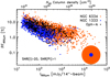Fig. 17 Comparison plot of PF as a function of I derived from BISTRO observations in three different regions: NGC 6334 in orange (this work, similar to the middle panel of Fig. 8), NGC 1333 in blue (Doi et al. 2020), and Oph-A in black (presented in Kwon et al. 2018, and also Furuya et al., in prep.). The concentric filled circles on the bottom right of the plot indicate the relative sizes of the regions corresponding to about 10, 2, and 0.2 pc in total extent, for NGC 6334, NGC 1333, and Oph-A, respectively. The angularresolution of the BISTRO data are 0.09, 0.02, and 0.01 pc in physical scales for NGC 6334, NGC 1333, and Oph-A, at the distance of 1.3 kpc, 299 pc, and 150 pc, respectively.

6.2 The B-field structure of a high-mass star forming hub-filament system

The B-field structure is on average perpendicular to the northern section (crest 4) of the main ridge of NGC 6334, which would suggest a formation process compatible with the theoretical model proposed by Inoue et al. (2018), where a filament is formed by the convergence of a flow of matter along the B-field lines hence forming a filament perpendicular to these lines (see also Inoue & Fukui 2013; Vaidya et al. 2013; Arzoumanian et al. 2018; Bonne et al. 2020). In this scenario, the flow of matter would be initially generated by the bending of the ambient B-field lines induced by an interstellar shock compression. Such a bent structure of the B-field lines around elongated molecular clouds is compatible with the observational findings of Tahani et al. (2018, 2019). Large scale CO molecular line observations have suggested that NGC 6334 may be located at the shock front of the collision between two clouds (Fukui et al. 2018).

The network of sub-filaments surrounding the ridge is connected to it in a roughly perpendicular orientation (see Fig. 13). The POS B-field is mostly perpendicular (or has a random orientation with respect) to the sub-filaments in their outer parts. In the inner parts, where the sub-filaments merge with the clump-hub, the relative orientation between the sub-filaments and the POS B-field angle becomes mostly parallel (see Figs. 13 and 14). This trend has also been found recently toward the G33.92+0.11 (Wang et al. 2020) and Serpens South (Pillai et al. 2020) hub-filament systems. This finding suggests that the sub-filaments may be formed orthogonal to the ambient B-field and then merged with the ridge, forming a clump-hub structure, due to, for instance, shock compression events, interstellar turbulence, or under the gravitational attraction by the ridge itself. Indeed, the whole region, encompassing the clump-hub and the sub-filaments (crests 5 to 10, 13, and 14), is virially bound with a total mass of ~ 7700 M_⊙ and total virial masses of ~ 300−1000 M_⊙, assuming a spherical geometry with an effective radius of ~1 pc and σ_v ~ 0.5−1.0 km s⁻¹.

In addition to a large-scale longitudinal velocity gradient observed in HCO⁺ along the ridge, some of the sub-filaments (as identified in Fig. 10) exhibit longitudinal velocity gradients perpendicular to the ridge (see Fig. 2 of Zernickel et al. 2013). ALMA high-resolution molecular line observationsof dense gas show also multiple velocity components along a section of the southern part of crest 4 (Shimajiri et al. 2019), that may be tracing dynamical interactions between the ridge and the surrounding sub-filaments. These velocity gradients may be tracing matter flowing onto the ridge and clump-hub, or the merging of the sub-filaments with the ridge. The B-field structure at the tip of the sub-filaments evolves under the influence of the gravitational potential of the clump-hub, while the B-field in the outer part of the sub-filaments still keeps the initial orientation, which better reflects the physical process leading to their formation. The variation of the B-field structure along the sub-filaments from their outer parts to their inner parts may be tracing and be coupled to these local velocity flows of matter in-falling onto the clump-hub, as also suggested by MHD simulations (Gómez et al. 2018).

Along crest 3 of the ridge, the B-field orientation varies from being mostly perpendicular to parallel to the crest (Fig. 12). Comparing with the velocity field derived from HCO⁺(3−2) molecular line data (Zernickel et al. 2013), this variation of the B-field structure may be induced by longitudinal motions along the crest, possibly by the gravitational potential of source III, a young cluster with high-mass stars. This variation of ${\chi }_{B_{\text{POS}}}$ observed toward the source III may also be due to the effect of feedback from the expansion of the UCH II region associated with this young high-mass star-forming site.

Figure 18 shows the variation of the polarization properties as two sub-filaments (crests 5 and 6) merge into a single filament (in projection at least) connected to the clump-hub. Transverse profiles of I and PI across the two separated crests 5 and 6 shows two peaks in I and is flat in PI (red curves in Fig. 18). The two peaks in the I profile show larger values and their separation gets smaller as the distance to the clump-hub shrinks. When the two crests are observed to merge (corresponding to the blue segments in Fig. 18-left), a single peak in I is seen, with a value ~4 times larger compared to the peak intensity when the two crests were separated. This increase in I toward the crests of the merged-filaments is larger than a simple addition of the intensity of the two separated-filaments, suggesting (1) this merging is not due to projection effects and integration along the LOS of two physically independent filaments, but (2) there is an additional efficient infall of matter onto the merged filaments (resulting in an increase in the density). We might be witnessing here the precursor of a core-hub. The PI profile across the merged filaments shows a dip (seen also in PF) at the position of the peak in I. The POS B-field angle across these two filaments also changes and is observed to be perpendicular to the crest after they merge, while the B-field lines are bent on both sides of the crest in a horseshoe pattern (Figs. 4 and 18). This correlation between the variation of the POS B-field structure and the dip in PI and PF may be tracing depolarization of the polarized emission due to the integration along the LOS or within the beam of unresolved B-field structures. Similar variations of the polarization properties can be seen along crest 8, which seems to be connected to the core-hub I(N) (see Figs. 4 and 13). These variations are also associated with an increase in the dispersion of χ_POS (cf., Fig. 7) suggesting the change of the geometry of the B-field as the sub-filaments merged with the clump- and core-hubs.

As can be seen in Table 2 and Fig. 15, the ridge and most of the sub-filaments of NGC 6334 are thermally supercritical with ${\alpha }_{\text{cyl}}^T<1$. Toward the ridge, both turbulent ${\alpha }_{\text{vir}}^v$ and magnetic ${\alpha }_{\text{vir}}^B$ virial parameters <1, suggesting that when taken separately the thermal, turbulent, or magnetic energy alone cannot support the ridge against gravity. Toward the sub-filaments, ${\alpha }_{\text{vir}}^v$ decreases and ${\alpha }_{\text{vir}}^B$ increases from their outer parts to their inner parts, suggesting stronger role of the gravity and magnetic field in the inner parts of the sub-filaments when they merge with the clump-hub. When all three main pressure forces are considered simultaneously, ${\alpha }_{\text{vir}}^{v,B}\gtrsim 1$, implying that while gravity is important in the evolution of and the interactions between the NGC 6334 filaments, the magnetic field as well as kinetic support play a key role in their overall energy balance.

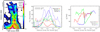Fig. 18 Left: Stokes I map of the northern region of NGC 6334 toward the sub-filaments 5 and 6 (see Fig. 10). The black lines correspond to ${\chi }_{B_{\text{POS}}}$ and their lengths are proportional to PF. On the right hand side, a vertical line indicates the 5% PF scale. The black filled circle indicates the 14′′ beam. The horizontal blue, green, and red lines show the (0.8 pc) cuts used to derive the profiles shown on the middle and right panels, for the merged, merging, and separated profiles, respectively. Middle: three transverse cuts, from east to west, where the sub-filaments are still separated (red), where they are merging (green), and where they are merged (blue) and not distinguishable any more as two peaks in Stokes I. Each profile has been averaged vertically between the two lines of the same color indicated on the left hand side plot. The solid and dashed line profiles show Stokes I and PI, respectively. We see a drop of PI toward the peak in I when the two filaments merge, that may be due to depolarization via beam-smearing of the B-field where the two sub-filaments merge. Right: same as the middle panel for the variation of ${\chi }_{{\text{B}}_{\text{POS}}}$ across the two sub-filaments.

6.3 Impact of the star formation feedback on the observed polarization properties

A main difficulty in the interpretation of polarization observations is that dust polarized emission depends on (1) the dust grain properties (size, shape, composition), (2) the efficiency of grain alignment with the local B-field, and (3) on the magnetic field structure (mean orientation with respect to the LOS and dispersion on the POS and along the LOS). In addition, the observed emission is integrated along the LOS and averaged within the observational beam. Thus understanding the origin of the variation of the polarization properties, such as the relation between the polarization fraction and the intensity (column density), cannot be gained without taking into account these effects simultaneously. For example, large PF values require well aligned grains and ordered B-field structures with optimal orientations with respect to the LOS, while low PF values may be due to a loss of grain alignment, variation of the grain properties, or a change of the B-field configuration. At the observed densities, the alignment efficiency of dust grains with the local B-field lines is independent from the absolute B-field strength. In addition, alignment itself is considered instantaneous given the dynamical timescales of the molecular cloud even when there are interactions and shock compressions between different density structures (Hildebrand 1988; Voshchinnikov 2012; Hoang & Lazarian 2016). The observed PF values, however, may be affected by the B-field strength due to the increase or decrease of depolarization from a turbulent or ordered B-field structure, respectively.

As mentioned earlier, NGC 6334 is actively forming stars and stellar clusters. The dense and cold molecular gas is affected by feedback from the high-mass stars formed along and next to the ridge. This region is hence an excellent laboratory to study the effect of feedback on the polarized dust emission properties and the B-field structure. While we refer the reader to a companion paper (Tahani et al., in prep.) for a detailed analysis, we give below a qualitative overview on the impact of the expanding H II regions on the surrounding B-field and polarized emission.

As an example of the impact of feedback, we note the POS B-field structure bends along the dense shell around the H II region corresponding to source II, where the expansion of the H II region has swept up most of the local dust and has created a cavity of submm continuum emission seen in our observations (cf., Fig. 19). This expansion likely influenced the pre-existing B-field structure, and the field was dragged along with the swept-up material. The cloud was reshaped into the now-observed shell with enhanced polarized emission due to an ordered B-field structure curved along the compressed shell (see, e.g., Tang et al. 2009; Planck Collaboration Int. XXXIV 2016, for similar discussions). A similar feedback effect may be seen toward the shell associated with the H II region to the south of source IV, albeit with a more complicated B-field structure and polarization pattern. Detailed 3D modeling is needed to understand the origin of these observed emission. This study will be partly addressed in Tahani et al. (in prep.).

The clump-hub shows another example of the impact of the feedback. Figure 20-top shows a scatter plot of PF as a function of I toward the clump-hub (black dashed ellipse in Fig. 19). All the data points toward the clump-hub have SNR(I) > 25 and SNR(PI) > 3. We see an overall decreasing trend of PF as a function of I (cf., Fig 8). A decrease in PF with I (or $N_{{\text{H}}_2}$) has been reported in previous studies and ascribed to the loss of grain alignment efficiency or the random component of the magnetic field (e.g., Jones et al. 1992, 2015; Whittet et al. 2001, 2008; Planck Collaboration Int. XIX 2015). Notably, the observed PF versus I data points from the clump-hub are not well described by a single mean power law. We can see that the linear fit log PF versus log$N_{{\text{H}}_2}$ for the data points with $N_{{\text{H}}_2}<2\times {10}^{22}{\text{cm}}^{-2}$ provides a best fit slope of − 0.72 ± 0.09, while for the data points with $N_{{\text{H}}_2}>2\times {10}^{22}{\text{cm}}^{-2}$ the fitted slope of − 0.14 ± 0.04 is much shallower. A fit to the upper envelope of the distribution yields a slope of − 0.29 ± 0.05. All of these slopes are shallower than the PF$\propto N_{{\text{H}}_2}{}^{-1}$ relation expected from the progressive loss of grain alignment expected in the framework of radiative torques (RAT) grain alignment theory due to the attenuation of the interstellar radiation field with increasing column density (e.g., Cho & Lazarian 2005; Lazarian 2007; Lazarian & Hoang 2007; Hoang & Lazarian 2014).

For these high column densities $N_{{\text{H}}_2}\gg {10}^{22}{\text{cm}}^{-2}$, the observed shallower slopes may be tracing an increase in the grain alignment efficiency due to the enhanced anisotropic radiation from newborn stars embedded in the clump-hub. Indeed, according to the RAT theory, anisotropic radiation from stars embedded in high-column density clumps increases the efficiency of grain alignment (Lazarian & Hoang 2007; Lee et al. 2020; Hoang et al. 2020), which may result in the observed shallower slopes (see also Pattle et al. 2019). Moreover, Hoang et al. (2019) show that when the intensity of the radiation from the embedded stars is large, the polarization fraction decreases due to the removal of large grains. We may be witnessing this effect toward the core-hubs (red data points in Fig. 20-top), which show a steep decrease of PF for $N_{{\text{H}}_2}\gtrsim {10}^{24}{\text{cm}}^{-2}$. This effect may also be seen in the bottom panel of Fig. 20, which traces the variations of PF and I across the two core-hubs. Toward the older source I, a trough in PF is associated with an increase in Stokes I. Toward the youngest source I(N), however, there is a spatial shift between the position of the dip in PF and the peak in I. Lower PF values are observed toward the edge of this latter source compared to larger PF values toward its high column density center. In the cut toward the source I, the emission from the ridge (crest 4) can also be seen (at ~ 1.6 pc from the x-axis in Fig. 20) which interestingly is not associated with a drop in PF, but with large PF values. The observed POS B-field toward the crest 4 embedded in the clump-hub has an ordered structure, which may be also contributing to the observed large PF values. The slopes derived from the PF versus I plot in Fig. 20-top are also shallower than the − 0.5 slope expected from a purely turbulent B-field (Jones et al. 2015; Andersson 2015), consistent with the observed ordered B-field structure toward the clump-hub (cf., e.g., Fig. 19).

In summary, the polarization features observed toward NGC 6334 may result from the impact of star formation feedback. Such features include: (1) the re-organization of the structure of the B-field on the scale of H II regions (within the compressed shells) where the mean B-field orientation is reoriented closer to the POS, (2) an increase in the B-field strength, ordering its structureand reducing depolarization due to integration of emission along the LOS and within the beam, (3) an increase in the efficiency of grain alignment with the local B-field due to an enhanced local radiation field from the newborn high-mass stars, and (4) a drop of polarization fraction toward the densest core-hubs due to the removal of large grains from stronger stellar feedback or a more tangled and unresolved configuration of the B-field.

Fig. 19 Zoom-in of the northern region of NGC 6334 (same as Fig. 13). The white lines show ${\chi }_{B_{\text{POS}}}$ and their lengths are proportional to PF. On the right hand side, a vertical line indicates the 10% PF scale. The black filled circle indicates the 14′′-beam. The black dashed ellipse shows the clump-hub. The two core-hubs I and I(N) are also indicated. The crosses and circles are the same as in Fig. 1-top-left.

Fig. 20 Properties observed toward the clump-hub (black dashed ellipse in Fig. 19). Top: PF as a function of I for SNR(I) > 25 and SNR(PI) > 3. The vertical small black lines show the statistical uncertainties on PF. The black, purple, and cyan lines indicate the best linear fits to the upper 95% percentiles of the distribution, the data points with $N_{{\text{H}}_2}<2\times {10}^{22}{\text{cm}}^{-2}$, and the datapoints with $N_{{\text{H}}_2}>2\times {10}^{22}{\text{cm}}^{-2}$, respectively.The best fit slopes are indicated on the plot. For comparision, the yellow and red lines indicate slopes of − 0.5 and − 1, respectively. Bottom: variation of PF (solid lines) and I (dashed lines) for two horizontal cuts from east to west, crossing the star forming regions I and I(N) in red and blue, respectively. The peak in I of the blue dashed profile at ~1.6 pc corresponds to the position of the ridge (crest 4).

Fig. 21 Results derived from the MHD numerical simulation presented by Inoue et al. (2018). The selected snapshot corresponds to t = 0.7 Myr after the filament formation by shock compression. The mass per unit length of the filament at this epoch is ~ 120 M⊙ pc−1. (a) Column density map of the filament. The black curve shows the crest of the filament traced with FilFinder (Koch & Rosolowsky 2015). (b) The small red lines indicate the POS B-field angle toward the same region shown in panel a. The black curve is the crest of the filament.(c)–(f) Power spectra of the column density, the POS B-field angle, the difference of the angle between the POS B-field orientation and the filament orientation, and the B-field strength, respectively. The slopes derived from the power law fits (shown in blue) to each of the power spectra are indicated on the panels. The vertical black dashed line indicates the highest frequency data point used to fit the power-law corresponding to 10 computational cells.

6.4 Understanding the origin of the slope of the B-field power spectrum

A recent analysis of the column density variations along the crest of a sample of filaments observed by Herschel in three star-forming clouds indicates that the 1D column density power spectra of these filaments are well defined by a power law function (down to Herschel resolution of ~ 0.02 pc) with a mean slope of − 1.6 ± 0.3 (Roy et al. 2015). This observed power law slope is compatible with the theoretical value suggested by Inutsuka (2001) close to twenty years ago to explain the origin of the Salpeter (1955) power-law slope of the IMF at the high-mass end. More recently, in an attempt to investigate the origin of the observed angular momentum of star-forming cores, Misugi et al. (2019) proposed a new theoretical model based on the filament velocity power spectrum. This model suggests that cylindrical filaments characterized by a 1D Kolmogorov velocity power spectrum slope of − 5∕3 will fragment into cores showing a distribution of angular momentum compatible with the observations.

The results presented by Roy et al. (2015) and Misugi et al. (2019) suggest that the column density (line mass) and velocity fluctuations along a filament may help to illuminate the origin of the IMF shape and the properties of the cores (e.g., angular momentum) formed from filament fragmentation. Since the gas and the magnetic field are dynamically well coupled in the ISM (i.e., frozen-in conditions), the magnetic field power spectrum should be related to the density and velocity power spectra and this link would depend on the physical processes resulting in the formation of the ISM structures. Thus, the observational determination of the power spectrum of the magnetic field configuration could provide valuable information on the origin of the formation of these structures and the link between the kinetic, magnetic, and gravitational energies at play in the ISM (see also Li & Burkert 2018 for a theoretical approach linking the power spectra of the density and magnetic energy fields in the ISM).

Here we presented for the first time the power spectrum of the B-field POS angles ${\chi }_{B_{\text{pos}}}$ observed along the NGC 6334 ridge (cf., Fig. 16). We show that the power spectrum of ${\chi }_{B_{\text{pos}}}$, similarly to the power spectrum of I, can also be well represented with a power law function and no characteristic scales are detected down to the resolution of the data. The slope of the power spectrum of ${\chi }_{B_{\text{pos}}}$, − 1.33 ± 0.23, is measured to be ~20% shallower than that of I (− 1.74 ± 0.27, cf., Fig. 16). We also presented the power spectrum of the difference of angle between ${\chi }_{B_{\text{pos}}}$ and the ridge crest orientation; θ_diff defined in the interval [0°, 90°]. This latter power spectrum has a slope of − 0.69 ± 0.34, shallower than the power spectrum slope of I and ${\chi }_{B_{\text{pos}}}$.

We compared this observational result with the power spectrum of the magnetic field angle along a supercritical filament formed in the MHD numerical simulation of Inoue et al. (2018). Figure 21 presents the power spectra of the column density, the POS B-field angle, and the difference between the POS B-field angle and the filament orientation derived from the 3D data cubes of this simulation. The slopes of the power spectra of the different quantities derived from the observations and the simulations are in agreement. This similarity suggests that the observed column density (line mass) and B-field fluctuations along the star forming NGC 6334 filament may be inherited from the filamentformation process and have a coupled evolution due to the accretion of matter and fragmentation under the interplay of the turbulent, gravitational, and B-field energies as incorporated in this MHD simulation. We also derive the power spectrum of the POS B-field intensity along the filament from the MHD simulation. This latter power spectrum has a power law slope similar to that of the POS B-field angle power spectrum, both ~ 20% shallower than that of I (cf., Fig. 21).

Following these preliminary results, we suggest that understanding the theoretical link between the power spectra of column density, velocity, and magnetic field (both angle and strength) and its evolution in time may lead to a new and independent method to infer the B-field strength from polarization observations, which do not provide a direct measurement of the B-field strength.

Here we presented the analysis of the power spectra of different quantities toward a single observed filament and a single simulated filament. Further detailed analysis of the column density and B-field fluctuations along statistical samples of both observed and simulated filaments are necessary to understand better the underlying physical processes captured by the observations.

7 Summary and conclusions

In this paper, we present the first BISTRO results of the JCMT/SCUBA-2/POL-2 observations at 850 μm toward the NGC 6334 high-mass star-forming hub-filament network. Our main results may be summarized as follows:

• BISTRO observations provide for the first time the submm polarization properties at high angular resolution (14′′ or 0.09 pc at 1.3 kpc distance) and high S/N (SNR(I) ≫ 25 and SNR(PI) ≫ 3) toward the 10 pc × 2 pc hub-filament network hosting a 10 pc-long ridge, sub-filaments, and core-hubs where stellar clusters and high-mass stars are forming (Figs. 1–4).

• The observations show a positive correlation between the polarized intensity PI and the total intensity I (PI ∝ I^{0.65 ± 0.02}), where both PI and I span ~3 orders of magnitude in polarized and total emission, respectively (Fig. 8-left). This correlation, however, exhibits a scatter by more than one order of magnitude in PI for I values spanning ~3 orders of magnitude. The observations show an overall negative correlation between the polarization fraction PF and I over ~3 orders of magnitude in PF with PF ∝ I^{−0.35 ± 0.02} (Fig. 8-middle). As for PI, a large scatter in PF (of ~2 orders of magnitude) is observed for a given value of I, with PF values as high as 6% for $N_{{\text{H}}_2}~{10}^{23}{\text{cm}}^{-2}$ (see also, Fig. 20-top). This indicates that the dust grains remain well-aligned with the B-field to the highest observedcolumn densities.

• The observed slope between the PF and I values (see previous paragraph) is shallower than the − 1 slope expected from the progressive loss of grain alignment due to the attenuation of the interstellar radiation field with increasing column density (i.e., from the RAT theory) and shallower than the − 0.5 slope expected from a purely turbulent B-field (see Fig. 20-top). In Sect. 6.3, we suggest that the large PF values observed toward NGC 6334 may be tracing ongoing feedback effects on the observed polarized dust emission that may result from the combination of (1) an enhanced radiation field from the newborn (high-mass) stars, (2) the re-organization of the structure of the B-field on the scale of H II regions (within compressed shells), and (3) the increase of the B-field strength ordering its structure and reducing depolarization due to the integration of emission along the LOS and within the beam.

• The ridge and the clump-hub structure are surrounded by sub-filaments (Fig. 10). In Sect. 4.2, we investigated the variation of the polarization and physical properties along the sub-filaments from their outer (out) to their inner (in) parts. In the outer parts, the POS B-field shows mostly perpendicular or random orientation with respect to the sub-filament crests. In their inner parts, where the sub-filaments are merging with the clump-hub, the B-field is parallel to their crests (cf., Fig. 13). This change of relative orientation along the sub-filaments may be due to material flowing along their crests onto the ridge and hubs. These flows of matter may drag the field lines, aligning them with the filament crests (cf., Sect. 6.2). The polarization fractions and the dispersion of the POS B-field angle are smaller on average in the inner parts of the sub-filaments compared to their outer parts (cf., Fig. 14).

• We also observe a variation in the stability of these sub-filaments (cf., Fig. 15). The kinetic virial parameter ${\alpha }_{\text{vir}}^v$ is on average smaller in the inner parts compared to the outer parts, while the magnetic virial parameter ${\alpha }_{\text{vir}}^B$ increases (by a factor of ~1.8 on average) from out to in. In the outer parts, ${\alpha }_{\text{vir}}^B~0.5\pm 0.3<1$ suggesting that the magnetic tension alone is not enough to balance gravity while the inner parts of the sub-filaments seem to be in a magnetic critical balance with ${\alpha }_{\text{vir}}^B~1$. When both the magnetic and kinetic (thermal and turbulent) supports are combined, the estimated ${\alpha }_{\text{vir}}^{v,B}\gtrsim 1$ values suggest that the sub-filaments are in an overall balance between the effective pressure forces and gravity (Sect. 4.2). This behavior is also seen along the ridge (Sect. 4.1).

• We identify a signature in the polarized emission toward two sub-filaments (with two spatially separated crests) that seem to be merging (as seen in dust continuum) to form a filament with a single crest (Fig. 18). We see the gradual increase of the total intensity due to the merging of the two sub-filaments and detect a drop in the polarized intensity toward the crest of the merged filaments. We suggest that this drop in PI (and PF), while I increases, is due to the depolarization from the integration along the LOS and within the beam of the unresolved B-field structures resulting from the merging of two different (partly independent) B-field structures along each of the initially separated filaments. This increase in I toward the crests of the merged-filaments is larger than a simple addition of the intensity of the two separated-filaments, suggesting efficient infall of matter onto the merged-crest. This behavior may be indicative of an early stage of a core-hub formation.

• We compare the properties observed toward NGC 6334 with two other regions observed as part of the BISTRO survey: Oph-A and NGC 1333 (Fig. 17). While these three regions have physical sizes that span 2 orders of magnitude in spatial scales, from ~0.2 to ~10 pc, they all show a similar scatter of PF values, of more than 2 orders of magnitude in PF (from ~0.2 to ~20%). This scatter is also observed for each I value, where a large scatter in I is also seen for a given value of PF. These observed similarities suggest that the self-similar description of the physical processes in a possibly fractal magnetized ISM also has an imprint in the dust polarized thermal emission (cf., Sect. 6.1).

• We present the first power spectrum of the POS B-field angles observed along the NGC 6334 ridge crest and compare it to the power spectrum of the intensity emission (cf., Fig. 16 and Sect. 5). The former is well represented by a power law function with a slope ~20% shallower than that of the latter. We compared this result with the power spectrum of filaments obtained from an MHD numerical simulation of massive filament formation (Fig. 21) and find consistent values. These preliminary results suggest that the structure of the column densities (line mass) and POS B-field angles along the NGC 6334 filament may be each inherited from the filament formation process and have a coupled evolution (cf., Sect. 6.4). Understanding the theoretical link between the power spectra of column density and magnetic field (POS angle and strength) may lead to a new and independent method to infer the B-field strength from polarization observations.

In this paper we have presented a first look at these rich BISTRO observations toward NGC 6334. The different topics addressed in Sect. 6 will be investigated in dedicated and in-depth forthcoming studies (e.g., Tahani et al., in prep.). To assess the reliability of the scenario presented above regarding the change of the properties along the sub-filaments and toward the clump-hub, large-scale molecular line mapping (at the appropriate resolutions) will be needed, to better understand the dynamics of these structures. The combination of the B-field structure observed at the BISTRO scale with that at higher angular resolution will also be very valuable to study the role of the B-field in the matter assembly and fragmentation processes that lead to the formation of massive stars. Quantitative comparisons with dedicated MHD numerical simulations will also be important to understand the physical processes at play in theses high-mass star-forming hub-filament systems.

Acknowledgements

D.A. acknowledges support by FCT/MCTES through national funds (PIDDAC) by the grants UID/FIS/04434/2019 & UIDB/04434/2020. This research is partially supported by Grants-in-Aid for Scientific Researches from the Japan Society for Promotion of Science (KAKENHI 19H0193810). C.L.H.H. acknowledges the support of the NAOJ Fellowship and JSPS KAKENHI grants 18K13586 and 20K14527. D.J. and J.D.F. are supported by the National Research Council of Canada and by Natural Sciences and Engineering Research Council of Canada (NSERC) Discovery Grants. P.M.K. acknowledges support from the Ministry of Science and Technology (MOST) grants MOST 108-2112-M-001-012 and MOST 109-2112-M-001-022 in Taiwan, and from an Academia Sinica Career Development Award. Y.D. acknowledges the support of JSPS KAKENHI grant 18H01250. K.Q. is partially supported by National Key R&D Program of China No. 2017YFA0402600, and acknowledges the National Natural Science Foundation of China (NSFC) grant U1731237. C.W.L. is supported by the Basic Science Research Program through the National Research Foundation of Korea (NRF) funded by the Ministry of Education, Science and Technology (NRF-2019R1A2C1010851). W.K. is supported by the New Faculty Startup Fund from Seoul National University and by the Basic Science Research Program through the National Research Foundation of Korea (NRF-2016R1C1B2013642). M.T. is supported by JSPS KAKENHI grants 18H05442,15H02063, and 22000005. J.K. is supported by JSPS KAKENHI grant 19K14775. This program is part of the JCMT BISTRO Large Program observed under project code M17BL011. Team BISTRO-J is in part financially supported by 260 individuals. The James Clerk Maxwell Telescope is operated by the East Asian Observatory on behalf of The National Astronomical Observatory of Japan; Academia Sinica Institute of Astronomy and Astrophysics; the Korea Astronomy and Space Science Institute; Center for Astronomical Mega-Science (as well as the National Key R&D Program of China with No. 2017YFA0402700). Additional funding support is provided by the Science and Technology Facilities Council of the United Kingdom and participating universities in the United Kingdom, Canada, and Ireland. Additional funds for the construction of SCUBA-2 and POL-2 were provided by the Canada Foundation for Innovation. The authors wish to recognize and acknowledge the very significant cultural role and reverence that the summit of Maunakea has always had within the indigenous Hawaiian community. We are most fortunate to have the opportunity to conduct observations from this mountain.

Appendix A Details on the quality assessments of the BISTRO data of NGC 6334

To complement the presentation of the data of the JCMT/SCUBA-2/POL-2 BISTRO observations at 850 μm toward the NGC 6334 field (see Sect. 2), we here present maps of the uncertainties of the total intensity I, the polarized intensity PI, polarization fraction PF, and POS B-field angle. These maps show the statistical uncertainties derived from the pol2map data reduction pipeline reprojected onto 12′′-pixel size grids⁹. Two DAISY maps have been observed toward the north and the south of the field and combined into a ~ 10 pc × 2 pc mosaic. The limits of the two subfields are indicated on the top-right hand side panel of Fig. A.1. The 6′ -diameter circles indicate the area where the observation pattern of the POL2-DAISY mode yields uniform noise coverage. Toward these areas of the map, the data have the lowest uncertainties (see Fig. A.1). The I map shows larger uncertainties toward the bright compact sources due to the increase of pointing and calibration uncertainties toward steep intensity gradients. We see larger uncertainties toward the edge of the maps and in the regions between the two subfields. These larger uncertainties on I (δI) can be seen on the right-hand side panel of Fig. A.2, which shows a scatter plot of δI as a function of I. For SNR(I) > 3, δI is mostly uniform with a mean value of ~ 1.6 mJy/14′′-beam. We see larger δI for the extreme I values ≳ 8 Jy/14′′-beam toward the bright compact sources (cf., Fig. A.1). More than 65 and 70% (2293 pixels) of the emission for SNR(I) > 3 and SNR(I) > 5, respectively, correspond to SNR(I) > 25. For SNR(I) > 25 (2293 pixels), 79% of the data points (1822 pixels) have SNR(PI) > 3. Only 4% (81 pixels) of the total pixels with SNR(PI) > 3 have SNR(I) < 25. This excellent overall S/N can be also seen on Fig. A.3 showing S/N contours over-plotted on the I and PI maps. For the analysis presented in this paper, we thus select data points with SNR(I) > 25 that correspond also mostly to data points with SNR(PI) > 3. The selection criteria on SNR(PI) is defined by the debiasing method that we use and which is shown to be reliable for SNR(PI) > 3 (cf., 2.2, Vaillancourt 2006; Plaszczynski et al. 2014).

Fig. A.1 Maps showing the distribution of the uncertainties derived for Stokes I, PI, PF, and ${\chi }_{B_{\text{POS}}}$ from left to right and top to bottom. The HPBW resolution of these maps is 14′′. The same emission area is plotted for all the four maps corresponding to SNR(I) > 25. The contours, which are the same for all the plots, correspond to I = 0.4, 1.4, and 8 Jy beam−1 or $N_{{\text{H}}_2}~(2,6,$and 37) × 1022 cm−2 (as in Fig. 1). The black dashed circles over-plotted on the PI map (top right) indicate the limits of the two observed DAISY subfields centered on (17:20:50.011, −35:45:34.33) and (17:20:19.902, −35:54:30.45) in (RA J2000, Dec J2000) for the north and south fields, respectively. The small and large red dashed circles have sizes of 6′ and 12′.

Fig. A.2 Left: measurement uncertainties on Stokes I as a functionof the signal on I. The black, yellow, and blue data points correspond to 3 < SNR(I) < 25, 25 < SNR(I) < 100, and SNR(I) > 100, respectively. The dashed and solid red lines show the median (1.24 mJy beam−1) and mean (1.57 mJy beam−1) uncertainties, respectively. Middle: uncertainties on PI as a function of PI for SNR(I) > 25. The black, yellow, and blue data points correspond to 0 < SNR(PI) < 3, 3 < SNR(PI) < 10, and SNR(PI) > 10, respectively. Right: uncertainties on the POS B-field angle, ${\chi }_{B_{\text{POS}}}$, as a functionof PF for SNR(I) > 25. The colors are the same as in the middle plot.

Fig. A.3 Left: Stokes I map at 850 μm observed with the JCMT/SCUBA-2/POL-2 toward NGC 6334. The HPBW resolution of this map is 14′′ and its pixel size is 4′′. The magenta, blue, cyan, and green contours are SNR(I) > 5, 10, 20, and 25, respectively. The SNR(I) = 25 correspond to I ~ 30 mJy beam−1 or $N_{{\text{H}}_2}~1.5\times {10}^{21}{\text{cm}}^{-2}$. Right: map of the polarized emission PI. The HPBW resolution of this map is 14′′ and its pixel size is 12′′. The magenta, blue, and cyan contours are SNR(PI) > 1, 3, and 5, respectively. The green contour corresponds to SNR(I) > 25 and is the same as in the left hand side panel.

Fig. A.4 Distribution of the signal of Stokes I (left), Q and U (middle) for SNR(I) > 25. The measured uncertainties on the three Stokes parameters are shown on the right hand plot.

Fig. A.5 Distributions of the uncertainties on PI (left), PF (middle), and ${\chi }_{B_{\text{POS}}}$ (right) for SNR(I) > 25 and SNR(PI) > 3 corresponding to the maps shown in Fig. A.1. Right hand side plot: different colors are as follow: blue for 3 < SNR(PI) < 5, orange for 5 < SNR(PI) < 10, and purple for SNR(PI) >10.

Figure A.4 shows the distribution of the observed Stokes parameters for SNR(I) > 25. The total intensity spans ~3 orders of magnitude showing the large intensity dynamic range of these observations from $N_{{\text{H}}_2}~{10}^{21}{\text{cm}}^{-2}$ to ~ 10²⁴ cm⁻². The Stokes Q and U values have asymmetric distributions about 0 with different shapes. The U distribution is skewed toward positive values. This distribution is compatible with a dominant POS B-field mostly at 45° + 90° = 135° with respect to the north direction (a peak in the histogram of ${\chi }_{B_{\text{POS}}}$ can be seen at ~130°, cf., Fig. 6). The mean and dispersion of the uncertainties of the I, Q, and U Stokes parameters are δI = (1.6 ± 1.8) mJy/14′′-beam, δQ = (1.13 ± 0.29) mJy/14′′-beam, and δU = (1.6 ± 0.30) mJy/14′′-beam (see Fig. A.4-right).

Figure A.5 shows the distributions of the uncertainties of PI, PF, and ${\chi }_{B_{\text{POS}}}$ for SNR(I) > 25 and SNR(PI) > 3. The mean and dispersion of the uncertainties of these distributions are δPI = (1.1 ± 0.3) mJy/14′′-beam, δPF = (0.2 ± 0.3) mJy/14′′-beam, and $\delta {\chi }_{B_{\text{POS}}}={(7\pm 1)}^{°},{(4\pm 1)}^{°},$ and ${(1.3\pm 0.8)}^{°}$ for data points with 3 < SNR(PI) < 5, 5 < SNR(PI) < 10, and SNR(PI) > 10, respectively.

Appendix B Column density and dust temperature maps of the NGC 6334 filament network

B.1 Column density and dust temperature

We derived the column density $(N_{{\text{H}}_2})$ map of the NGC 6334 field observed by BISTRO from the total intensity Stokes I map, with the relation $$N_{{\text{H}}_2}=I_{850}/(B_{850}[T]{\kappa }_{850}{\mu }_{{\text{H}}_2}{m}_{\text{H}}),$$(B.1)

where κ₈₅₀ = 0.0182 cm² g⁻¹ is the dust opacity per unit mass of dust + gas at 850 μm (e.g., Ossenkopf & Henning 1994), ${\mu }_{{\text{H}}_2}=2.8$ is the meanmolecular weight per hydrogen molecule (e.g., Kauffmann et al. 2008), m_H is the mass of a hydrogen atom, and B₈₅₀[T] is the Planck function for a given temperatureT.

Figure B.1-left, shows the dust temperature map of this region derived from gray-body fits to the Herschel five wavelength data presented in Russeil et al. (2013). As can be seen in this latter figure, in the northeast section of the NGC 6334 filamentary structure (e.g., crests 4, 5, 6, and 7), which is the least affected by the heating from the multiple H II bubbles present in the field (Russeil et al. 2016), the dust temperature is T_dust ~ 20 K. Toward the southern parts, the dust temperatures derived from the LOS integrated Herschel emission reach values up to ~30 K, which possibly trace the emission of warmer dust grains located mostly in the outer layers of the cloud. The dust temperatures (> 25 K) derived from Herschel data in these regions may not provide a good estimate of the gas temperature of the cold and dense molecular cloud traced with the 850 μm emission of the BISTRO data.

We thus derived a column density map, $N_{{\text{H}}_2}{}^{T=20\text{K}}$, for a constant T = 20 K corresponding to the dominent temperature observed toward the northern part of the NGC 6334 molecular cloud that is less affected by the warm H II regions. Temperatures of about 20 K are also compatible with the kinetic temperature toward star forming high-mass filaments and hubs derived from NH₃ GBT observations of the KEYSTONE project (Keown et al. 2019).

For completeness, we also derived a column density map, $N_{{\text{H}}_2}{}^{{\text{T}}_{\text{dust}}^{Herschel}}$, using the Herschel dust temperature map at a resolution of 36′′ (Russeil et al. 2013, and Fig. B.1-left) to compare with $N_{{\text{H}}_2}{}^{\text{T}=20\text{K}}$. The distribution of the $N_{{\text{H}}_2}{}^{\text{T}=20\text{K}}/N_{{\text{H}}_2}{}^{{\text{T}}_{\text{dust}}^{Herschel}}$ ratio of these two maps, toward the field observed by BISTRO with SNR(I) > 25, is shown in the right panel of Fig. B.1. This distribution is narrow, with a mean of 1.32 and a standard deviation of 0.35. The difference between the two maps, $N_{{\text{H}}_2}{}^{\text{T}=20\text{K}}$ and $N_{{\text{H}}_2}{}^{{\text{T}}_{\text{dust}}^{Herschel}}$, of about 30% on average is mostly smaller than the dispersion of the $N_{{\text{H}}_2}{}^{\text{T}=20\text{K}}$ found along the different crests studied in the paper (cf., Col. (2) of Table 2).

Fig. B.1 Left: dust temperature $T_{\text{dust}}^{Herschel}$ map (Russeil et al. 2013) derived from Herschel data observed as part of the HOBYS key program (Motte et al. 2010). This map is at the resolution of 36′′. The contours (corresponding to I = 0.4, 1.4, and 8 Jy beam−1 of the BISTRO data), the crosses, and the circles are the same as in Fig. 1-top-left. The Herschel (36′′) and BISTRO (14′′) beams are shown on the left bottom of the plot as concentric filled white and black circles, respectively. Right: distribution of the ratio $N_{{\text{H}}_2}{}^{\text{T}=20\text{K}}/N_{{\text{H}}_2}{}^{{\text{T}}_{\text{dust}}^{Herschel}}$ (see Appendix B.1 describing the derivation of the two quantities). The mean value of this distribution is 1.3, as indicated by the vertical line.

Fig. B.2 Left: comparing the column density values derived from ArTéMiS+SPIRE ($N_{{\text{H}}_2}{}^{\text{Art+SPIRE}}$ ) at 350 μm (from André et al. 2016) and BISTRO ($N_{{\text{H}}_2}{}^{\text{BISTRO}}$) at 850 μm (see Appendix B.2 for the expression used to estimate the column density from the observed total intensity). The vertical blue line indicates $N_{{\text{H}}_2}=3\times {10}^{22}{\text{cm}}^{-2}$ above which the two maps agree within a factor <2. The oblique black solid and dashed lines show the y = x and y = 2x relations. Middle: radial column density profiles (in log scale) perpendicular to and averaged along the 10 pc NGC 6334 elongated structure (i.e., crests from 1 to 5 in Fig. 10). The solid black and red lines correspond to the average profiles derived from ArTéMiS+SPIRE and BISTRO data, respectively. The purple dashed curve corresponds to $N_{{\text{H}}_2}{}^{\text{Art+SPIRE}}-N_{{\text{H}}_2}{}^{\text{Galactic}}$, where $N_{{\text{H}}_2}{}^{\text{Galactic}}=3\times {10}^{22}{\text{cm}}^{-2}$ correspondsto the large scale “Galactic emission” filtered out in the BISTRO maps. The angular resolution of the data isindicated by the blue dashed Gaussian function. Right: mean profiles (in linear scale) of the ratios $N_{{\text{H}}_2}{}^{\text{Art+SPIRE}}/N_{{\text{H}}_2}{}^{\text{BISTRO}}$ (black) and $(N_{{\text{H}}_2}{}^{\text{Art+SPIRE}}-N_{{\text{H}}_2}{}^{\text{Galactic}})/N_{{\text{H}}_2}{}^{\text{BISTRO}}$ (blue). The mean value of this latter ratio is ~1.5 indicated bythe horizontal line.

Thus, for the analysis presented in this paper, we derived the column density using a constant dust temperature of 20 K.

B.2 Comparison of BISTRO data with Herschel/SPIRE+ArTéMiS data

Here we compare the BISTRO observations at 850 μm with observations toward the same region obtained by Herschel/SPIRE (Motte et al. 2010) combined with ArTéMiS data at 350 μm at 8′′ resolution (André et al. 2016).

To compare the two observations at different wavelengths, we estimated the column density from the total intensity Stokes I values with the dust opacity per unit mass of dust + gas κ₈₅₀ = 0.0182 cm² g⁻¹ for the BISTRO data at 850 μm and κ₃₅₀ = 0.1 cm² g⁻¹ for the Herschel/SPIRE+ArTéMiS data at 350 μm (Ossenkopf & Henning 1994; Kauffmann et al. 2008). For both maps, we used a mean dust temperature of T = 20 K as explainedabove and also adopted by André et al. (2016).

Figure B.2 shows the column density values derived from BISTRO 850 μm data and those derived from SPIRE+ArTéMiS data at 350 μm data smoothed to the same resolution of 14′′. For column densities ≳3 × 10²² cm⁻² both maps agree within a factor < 2 (Fig. B.2-left).

We derived mean radial profiles perpendicular to the main axis of the elongated filament and averaged along its length. In practice, the maps have first been rotated by 30° (corresponding to the mean orientation of NGC 6334 on the plane-of-the-sky) from east to north. Second, horizontal cuts, perpendicular to the main axis of NGC 6334 have been averaged from south to north along the 10 pc structure. Figure B.2-middle shows the mean radial column density profiles perpendicular to the NGC 6334 cloud. For $N_{{\text{H}}_2}\gtrsim 3\times {10}^{22}{\text{cm}}^{-2}$ the mean ratio between the two profiles is ~1.6. For $N_{{\text{H}}_2}<3\times {10}^{22}{\text{cm}}^{-2}$, corresponding to scales r ≳ 0.3 pc from the central part of the filament, the ratio $N_{{\text{H}}_2}{}^{\text{Art+SPIRE}}/N_{{\text{H}}_2}{}^{\text{BISTRO}}$ increases up to values of ~10 for r ~1 pc or r ~2.′6 (Fig. B.2-right).

The drop of the observed emission of the BISTRO data compared to the emission observed by Herschel may be due to the removal of the large scale emission affecting the JCMT ground based data while Herschel data are in principle not affected by this problem.

Since NGC 6334 is located within 0.6 deg of the Galactic Plane, the emission is affected by large-scale “Galactic emission”, which corresponds to background and foreground emission ($N_{{\text{H}}_2}~3\times {10}^{22}{\text{cm}}^{-2}$) observed along the LOS in the surrounding of the NGC 6334 molecular cloud. We estimated here that “Galactic emission” to be $N_{{\text{H}}_2}~3\times {10}^{22}{\text{cm}}^{-2}$.

We hence compared the column density derived from BISTRO data with the “Galactic emission” subtracted column density values of the SPIRE+ArTéMiS data. As can be seen in Fig. B.2-middle and left, these “Galactic emission” column density subtracted SPIRE+ArTéMiS data are compatible within ~ 50% with the column density derived from BISTRO observations at 850 μm down to $N_{{\text{H}}_2}~{10}^{21}{\text{cm}}^{-2}$.

We thus conclude that our BISTRO data trace the intrinsic emission of the molecular cloud of NGC 6334 filtering out the large-scale emission on the orderof $N_{{\text{H}}_2}~3\times {10}^{22}{\text{cm}}^{-2}$ corresponding, in this case, to a combination of extended emission physically linked to the NGC 6334 molecular complex and to LOS foreground and background Galactic emission.

Appendix C Tests on the power spectrum analysis

The observations show a well defined power law shape of the power spectra of I, ${\chi }_{B_{\text{POS}}}$, and ϕ_diff (cf., 16). To check whether such well-defined power law power spectra could be the result of uncorrelated emission, we randomly reordered the observed data along the crest of the studied filament and derived the power spectrum for 50 realisations of test-data. Figure C.1-left shows an example of the power spectrum derived from one of the realisations. These power spectra are not well represented by power laws. Figure C.1-right shows the histogram of the slopes measured by fitting the test power spectra for the 50 realisations. The derived slopes are compatible with a flat spectrum. We hence conclude that the observed power spectra with well defined power law shapes are a result of the correlated fluctuations of these properties along the filament crest.

Fig. C.1 Left: a power spectrum example of the test data (intensity in red, POS B-field angle in purple, and difference angle in yellow), where the observed values along the ridge crest are randomly reordered. The vertical line shows the spatial resolution of the data. The data points have pixel size of 4′′. The straight colored lines show the best power-law fits to the power spectra and the derived power-law indexes (α) are shown on the bottom left hand side of the plot. Right: histogram of α for 50 realisations of random reorganization of the observed values. The vertical dashed lines indicate the derived power spectrum slopes from the observed values (see Fig. 16).

References

All Tables

All Figures

Fig. 1 Stokes parameter maps of the total I (top-left) and the polarized Q and U (bottom-left and -right, respectively) thermal dust emission at 850 μm observed with the JCMT SCUBA-2/POL-2 toward NGC 6334 as part of the BISTRO survey. Top right hand side panel: map of the (debiased) polarized emission, PI. The half-power-beam-width (HPBW) resolution of these maps is 14′′. For all maps,the plotted emission corresponds to SNR(I) > 25. The contours, which are the same for all plots, correspond to I = 0.4, 1.4, and 8 Jy beam−1 or $N_{{\text{H}}_2}~(2,6,$and 37) × 1022 cm−2. The lowest contour of I = 0.4 Jy beam−1 is equivalent to SNR(I) ~ 300 and SNR(PI) ~ 10. The white crosses on the I map indicate the seven high-mass star-forming regions numbered from I to V from north to south in addition to I(N) and E in the north of the field. The white circles show the positions and sizes of UCH II and H II regions (see Persi & Tapia 2008,and references therein).

In the text

	Fig. 2 Maps of the POS B-field angle ${\chi }_{B_{\text{POS}}}$ (left) and of the polarization fraction PF (right). The HPBW resolution of the maps is 14′′. The plotted emission correspond to SNR(I) > 25. The contours are I = 0.4, 1.4, and 8 Jy beam−1, as in Fig. 1.
In the text

	Fig. 3 Total intensity Stokes I map (same as Fig. 1-top left). The blue short lines (all with the same length) show the orientation of the POS B-field angle (${\chi }_{B_{\text{POS}}}$) for SNR(I) > 25 and SNR(PI) > 3. The contours are I = 0.4, 1.4, and 8 Jy beam−1, as in Fig. 1.
In the text

	Fig. 4 Polarized intensity (PI) map (cf., Fig. 1-top right). The blue short lines show the orientation of the POS B-field angle (cf., Fig. 3) and their lengths are proportional to the polarization fraction. A line showing a polarization fraction of 10% is indicated on the plot. The contours are I = 0.4, 1.4, and 8 Jy beam−1, as in Fig. 1.
In the text

Fig. 5 Planck total intensity Ip map of the 850 μm emission toward NGC 6334. The red contours show the Planck intensity at Ip ~ 48, 60, and 80 MJy sr−1 (at 5′ resolution) and the blue contour the BISTRO intensity 0.4 Jy/14′′-beam or 75 MJy sr−1 (at 14′′ resolution). The black lines are the POS B-field angles derived from Planck data at the resolution of 5′. The Planck (5′) and BISTRO (14′′) beams are shown on the right hand side of the plot as concentric filled white and black circles, respectively. The Galactic Plane is also indicated.

In the text

Fig. 6 Top: distribution of ${\chi }_{B_{\text{POS}}}$. The blue dashed line at 30° indicates themean position angle (θfil) of NGC 6334. The red solid line at 130° shows the mean ${\chi }_{B_{\text{POS}}}^{\text{p}}$ derived fromPlanck data (at the resolution of 5′) toward the field observed with BISTRO (cf., Fig. 5). Bottom: distribution of the polarization fraction PF. The solid and dashed blue lines indicate the mean and median values of PF at 14′′, respectively. The solid red line shows the mean PFp value derived from Planck data at 5′ resolution toward the BISTRO field.

In the text

	Fig. 7 Map of S (dispersion function of ${\chi }_{B_{\text{POS}}}$, see Eq. (4)) for SNR(I) > 25 and SNR(PI) > 3. The contours are I = 0.4, 1.4, and 8 Jy beam−1, as in Fig. 1.
In the text

Fig. 8 Top: PI versus I for SNR(I) > 25. The light and dark blue symbols are data points with 1 <SNR(PI) < 3 and SNR(PI) > 3, respectively. The dots correspond to 12′′ pixels. The red solid curve shows the median log(PI) per bin of log(I). The lower and the upper dashed red lines show the 16% and 84% percentiles, respectively. The black solid line is a linear fit to the distribution for SNR(PI) > 3 and I > 150 mJy beam−1 (indicated by the dotted vertical line). The value of the slope is given on the plot. The black dashed line is a linear fit to the upper 95% percentiles (see Sect. 3.3). The upper x-axis gives an estimate of the $N_{{\text{H}}_2}$ column density (see Sect. 2.3). Bottom: PF versus I. The dots, curves, and colors are the same as the upper plot for PF versus I.

In the text

Fig. 9 Scatter plot of S (dispersion function of ${\chi }_{B_{\text{POS}}}$) as a functionof I (top) and PF (bottom) for data points with SNR(I) > 25 and SNR(PI) > 3 (cf., Fig. 7). The data points with 50 < PI < 100 mJy beam−1 and PI > 100 mJy beam−1 are shown in yellow and red, respectively. The black solid curves show the median log(S) per bin of log(I) and log(PF) in the top and bottom panels, respectively. The lower and the upper dashed black lines are the 16% and 84% percentiles of the distributions, respectively. The red horizontal line at S = 52° shows the value that S would take for a B-field dominated by turbulence. Bottom panel: cyan solid line is a linear fit to the distribution.

In the text

Fig. 10 Crests of the identified filamentary structures over-plotted on the Stokes I map. The connected sections from 1 to 4 trace the ridge crest (cf., Figs. 11 and 12). The blue lines from 5 to 14 trace the crests of the sub-filaments. The cyan line traces the crest of a filament connecting the two core-hubs, I and I(N). The black dashed rectangle indicates the hub-filament structure (see Fig. 13). The black dashed ellipse shows the clump-hub. The crosses and circles are the same as in Fig. 1-top-left.

In the text

Fig. 11 Observed I (top), PI (middle), and PF (bottom) along the ridge crest for the sections from 1 to 4 (indicated with different colors, see Fig. 10) from south to north (left to right on the horizontal axes). The short vertical black bars show the ± σ statistical uncertainties. The horizontal black segments on the top right hand of the panels indicate the 14′′ (0.09 pc) beam size of the data. The blue curve on the top panel is the column density derived from SPIRE+ArTéMiS data after subtraction of a constant “Galactic emission” value of 3 × 1022 cm−2 (cf. Sect. 2.3). The blue curves on the middle and bottom panels show I along the ridge crest (same as the colored curve on the top panel).

In the text

Fig. 12 Variation of the position angles of ${\chi }_{B_{\text{POS}}}$ (green in thetop and red in the bottom), θfil (black), and ${\varphi }_{\text{diff}}=|{\theta }_{\text{fil}}-{\chi }_{B_{\text{pos}}}|$ (blue) along crests 3 (top) and 4 (bottom), from south to north. Only pixels along the crests are considered. The dotted horizontal lines show an angle of 90°. The vertical red line in the top panel is the position of source III (cf., Fig. 10). The horizontal black segments on the top right hand of the panels indicate the 14′′ (0.09 pc) beam size of the data.

In the text

Fig. 13 Close-up of the northern region of NGC 6334 within the black dashed rectangle indicated in Fig. 10. The crests are those shown in Fig. 10 and over-plotted on the Stokes I map. The white lines correspond to ${\chi }_{B_{\text{POS}}}$ and their lengths are proportional to PF. On the right hand side, a vertical line shows the 10% polarization fraction scale. The black filled circle corresponds to the 14′′ beam. The blue and red lines indicate the mean values for ${\chi }_{B_{\text{POS}}}$ for the out and in parts of the sub-filaments, respectively. The cyan lines show the orientation (θfil) of the out and in parts of the sub-filaments (see Sect. 4.2, Fig. 14, and Table 1). The length of the blue, red, and cyan lines is equal to 60′′, corresponding to the extent of the circular area used to estimate the parameters.

In the text

References

- Andersson, B. G. 2015, Magnetic Fields in Diffuse Media, eds. A. Lazarian, E. M. de Gouveia Dal Pino, & C. Melioli (Berlin: Springer), 407, 59 [Google Scholar]
- Andersson, B. G., Lazarian, A., & Vaillancourt, J. E. 2015, ARA&A, 53, 501 [NASA ADS] [CrossRef] [Google Scholar]
- André, P., Men’shchikov, A., Bontemps, S., et al. 2010, A&A, 518, L102 [NASA ADS] [CrossRef] [EDP Sciences] [Google Scholar]
- André, P., Di Francesco, J., Ward-Thompson, D., et al. 2014, Protostars and Planets VI (Tucson, AZ: University of Arizona Press), 27 [Google Scholar]
- André, P., Revéret, V., Könyves, V., et al. 2016, A&A, 592, A54 [NASA ADS] [CrossRef] [EDP Sciences] [Google Scholar]
- André, P., Arzoumanian, D., Könyves, V., Shimajiri, Y., & Palmeirim, P. 2019, A&A, 629, L4 [CrossRef] [EDP Sciences] [Google Scholar]
- Arzoumanian, D., André, P., Didelon, P., et al. 2011, A&A, 529, L6 [CrossRef] [EDP Sciences] [Google Scholar]
- Arzoumanian, D., André, P., Peretto, N., & Könyves, V. 2013, A&A, 553, A119 [NASA ADS] [CrossRef] [EDP Sciences] [Google Scholar]
- Arzoumanian, D., Shimajiri, Y., Roy, A., et al. 2017, Mem. Soc. Astron. It., 88, 720 [Google Scholar]
- Arzoumanian, D., Shimajiri, Y., Inutsuka, S.-i., Inoue, T., & Tachihara, K. 2018, PASJ, 70, 96 [NASA ADS] [CrossRef] [Google Scholar]
- Arzoumanian, D., André, P., Könyves, V., et al. 2019, A&A, 621, A42 [NASA ADS] [CrossRef] [EDP Sciences] [Google Scholar]
- Bastien, P., Bissonnette, E., Simon, A., et al. 2011, ASP Conf. Ser., 449, 68 [Google Scholar]
- Bonne, L., Bontemps, S., Schneider, N., et al. 2020, A&A, 644, A27 [EDP Sciences] [Google Scholar]
- Chandrasekhar, S., & Fermi, E. 1953, ApJ, 118, 113 [NASA ADS] [CrossRef] [Google Scholar]
- Chapin, E. L., Berry, D. S., Gibb, A. G., et al. 2013, MNRAS, 430, 2545 [NASA ADS] [CrossRef] [Google Scholar]
- Chen, H.-R., Rao, R., Wilner, D. J., & Liu, S.-Y. 2012, ApJ, 751, L13 [NASA ADS] [CrossRef] [Google Scholar]
- Chen, H.-R. V., Zhang, Q., Wright, M. C. H., et al. 2019, ApJ, 875, 24 [NASA ADS] [CrossRef] [Google Scholar]
- Chibueze, J. O., Omodaka, T., Handa, T., et al. 2014, ApJ, 784, 114 [NASA ADS] [CrossRef] [Google Scholar]
- Cho, J., & Lazarian, A. 2005, ApJ, 631, 361 [NASA ADS] [CrossRef] [Google Scholar]
- Coudé, S., Bastien, P., Houde, M., et al. 2019, ApJ, 877, 88 [NASA ADS] [CrossRef] [Google Scholar]
- Cox, N. L. J., Arzoumanian, D., André, P., et al. 2016, A&A, 590, A110 [NASA ADS] [CrossRef] [EDP Sciences] [Google Scholar]
- Crutcher, R. M. 2012, ARA&A, 50, 29 [NASA ADS] [CrossRef] [Google Scholar]
- Crutcher, R. M., Nutter, D. J., Ward-Thompson, D., & Kirk, J. M. 2004, ApJ, 600, 279 [NASA ADS] [CrossRef] [Google Scholar]
- Currie, M. J., Berry, D. S., Jenness, T., et al. 2014, ASP Conf. Ser., 485, 391 [Google Scholar]
- Davis, Jr. L., & Greenstein, J. L. 1951, ApJ, 114, 206 [Google Scholar]
- Dempsey, J. T., Friberg, P., Jenness, T., et al. 2013, MNRAS, 430, 2534 [Google Scholar]
- Doi, Y., Hasegawa, T., Furuya, R. S., et al. 2020, ApJ, 899, 28 [Google Scholar]
- Falceta-Gonçalves, D., Lazarian, A., & Kowal, G. 2008, ApJ, 679, 537 [NASA ADS] [CrossRef] [Google Scholar]
- Falceta-Gonçalves, D., Lazarian, A., & Kowal, G. 2009, Rev. Mex. Astron. Astrofis. Conf. Ser., 36, 37 [Google Scholar]
- Fiege, J. D., & Pudritz, R. E. 2000, MNRAS, 311, 85 [NASA ADS] [CrossRef] [Google Scholar]
- Fischera, J., & Martin, P. G. 2012, A&A, 542, A77 [NASA ADS] [CrossRef] [EDP Sciences] [Google Scholar]
- Friberg, P., Bastien, P., Berry, D., et al. 2016, SPIE Conf. Ser., 9914, 991403 [Google Scholar]
- Fukui, Y., Kohno, M., Yokoyama, K., et al. 2018, PASJ, 70, S41 [NASA ADS] [Google Scholar]
- Gómez, G. C., Vázquez-Semadeni, E., & Zamora-Avilés, M. 2018, MNRAS, 480, 2939 [Google Scholar]
- Le Gouellec, V. J. M., Maury, A. J., Guillet, V., et al. 2020, A&A, 644, A11 [EDP Sciences] [Google Scholar]
- Hacar, A., Tafalla, M., Kauffmann, J., & Kovács, A. 2013, A&A, 554, A55 [NASA ADS] [CrossRef] [EDP Sciences] [Google Scholar]
- Hacar, A., Tafalla, M., Forbrich, J., et al. 2018, A&A, 610, A77 [NASA ADS] [CrossRef] [EDP Sciences] [Google Scholar]
- Heitsch, F., Zweibel, E. G., Mac Low, M.-M., Li, P., & Norman, M. L. 2001, ApJ, 561, 800 [NASA ADS] [CrossRef] [Google Scholar]
- Hennebelle, P., & Inutsuka, S.-i. 2019, Front. Astron. Space Sci., 6, 5 [NASA ADS] [CrossRef] [Google Scholar]
- Hennemann, M., Motte, F., Schneider, N., et al. 2012, A&A, 543, L3 [NASA ADS] [CrossRef] [EDP Sciences] [Google Scholar]
- Hildebrand, R. H. 1983, QJRAS, 24, 267 [NASA ADS] [Google Scholar]
- Hildebrand, R. H. 1988, QJRAS, 29, 327 [NASA ADS] [Google Scholar]
- Hildebrand, R. H., Davidson, J. A., Dotson, J. L., et al. 2000, PASP, 112, 1215 [NASA ADS] [CrossRef] [Google Scholar]
- Hill, T., Motte, F., Didelon, P., et al. 2011, A&A, 533, A94 [NASA ADS] [CrossRef] [EDP Sciences] [Google Scholar]
- Hoang, T., & Lazarian, A. 2014, MNRAS, 438, 680 [NASA ADS] [CrossRef] [Google Scholar]
- Hoang, T., & Lazarian, A. 2016, ApJ, 831, 159 [NASA ADS] [CrossRef] [Google Scholar]
- Hoang, T., Tram, L. N., Lee, H., & Ahn, S.-H. 2019, Nat. Astron., 3, 766 [Google Scholar]
- Hoang, T., Tram, L. N., Lee, H., Diep, P. N., & Bich Ngoc, N. 2020, ApJ, submitted [Google Scholar]
- Holland, W. S., Bintley, D., Chapin, E. L., et al. 2013, MNRAS, 430, 2513 [NASA ADS] [CrossRef] [Google Scholar]
- Hull, C. L. H., & Plambeck, R. L. 2015, J. Astron. Instrum., 4, 1550005 [CrossRef] [Google Scholar]
- Inoue, T., & Fukui, Y. 2013, ApJ, 774, L31 [NASA ADS] [CrossRef] [Google Scholar]
- Inoue, T., Hennebelle, P., Fukui, Y., et al. 2018, PASJ, 70, S53 [NASA ADS] [Google Scholar]
- Inutsuka, S.-i. 2001, ApJ, 559, L149 [Google Scholar]
- Inutsuka, S., & Miyama, S. M. 1997, ApJ, 480, 681 [NASA ADS] [CrossRef] [Google Scholar]
- Jackson, J. M., Rathborne, J. M., Foster, J. B., et al. 2013, PASA, 30, e057 [NASA ADS] [CrossRef] [Google Scholar]
- Jones, R. V., & Spitzer, Jr. L. 1967, ApJ, 147, 943 [NASA ADS] [CrossRef] [Google Scholar]
- Jones, T. J., Klebe, D., & Dickey, J. M. 1992, ApJ, 389, 602 [NASA ADS] [CrossRef] [Google Scholar]
- Jones, T. J., Bagley, M., Krejny, M., Andersson, B.-G., & Bastien, P. 2015, AJ, 149, 31 [NASA ADS] [CrossRef] [Google Scholar]
- Juárez, C., Girart, J. M., Zamora-Avilés, M., et al. 2017, ApJ, 844, 44 [NASA ADS] [CrossRef] [Google Scholar]
- Kainulainen, J., Stutz, A. M., Stanke, T., et al. 2017, A&A, 600, A141 [NASA ADS] [CrossRef] [EDP Sciences] [Google Scholar]
- Kauffmann, J., Bertoldi, F., Bourke, T. L., Evans, II, N. J., & Lee, C. W. 2008, A&A, 487, 993 [NASA ADS] [CrossRef] [EDP Sciences] [Google Scholar]
- Keown, J., Di Francesco, J., Rosolowsky, E., et al. 2019, ApJ, 884, 4 [Google Scholar]
- Kirk, H., Myers, P. C., Bourke, T. L., et al. 2013a, ApJ, 766, 115 [NASA ADS] [CrossRef] [Google Scholar]
- Kirk, J. M., Ward-Thompson, D., Palmeirim, P., et al. 2013b, MNRAS, 432, 1424 [NASA ADS] [CrossRef] [Google Scholar]
- Koch, E. W., & Rosolowsky, E. W. 2015, MNRAS, 452, 3435 [NASA ADS] [CrossRef] [Google Scholar]
- Koch, P. M., Tang, Y.-W., Ho, P. T. P., et al. 2018, ApJ, 855, 39 [NASA ADS] [CrossRef] [Google Scholar]
- Könyves, V., André, P., Men’shchikov, A., et al. 2015, A&A, 584, A91 [NASA ADS] [CrossRef] [EDP Sciences] [Google Scholar]
- Könyves, V., André, P., Arzoumanian, D., et al. 2020, A&A, 635, A34 [CrossRef] [EDP Sciences] [Google Scholar]
- Kraemer, K. E., & Jackson, J. M. 1999, ApJS, 124, 439 [NASA ADS] [CrossRef] [Google Scholar]
- Kumar, M. S. N., Palmeirim, P., Arzoumanian, D., & Inutsuka, S. I. 2020, A&A, 642, A87 [EDP Sciences] [Google Scholar]
- Kwon, J., Doi, Y., Tamura, M., et al. 2018, ApJ, 859, 4 [NASA ADS] [CrossRef] [Google Scholar]
- Lazarian, A. 2007, J. Quant. Spectr. Rad. Transf., 106, 225 [NASA ADS] [CrossRef] [Google Scholar]
- Lazarian, A., & Hoang, T. 2007, MNRAS, 378, 910 [Google Scholar]
- Lazarian, A., Goodman, A. A., & Myers, P. C. 1997, ApJ, 490, 273 [NASA ADS] [CrossRef] [Google Scholar]
- Lazarian, A., Andersson, B. G., & Hoang, T. 2015, Grain alignment: Role of radiative torques and paramagnetic relaxation, 81 [Google Scholar]
- Lee, H. M., & Draine, B. T. 1985, ApJ, 290, 211 [NASA ADS] [CrossRef] [Google Scholar]
- Lee, H., Hoang, T., Le, N., & Cho, J. 2020, ApJ, 896, 44 [Google Scholar]
- Li, G.-X., & Burkert, A. 2018, MNRAS, 474, 2167 [Google Scholar]
- Li, H., Griffin, G. S., Krejny, M., et al. 2006, ApJ, 648, 340 [NASA ADS] [CrossRef] [Google Scholar]
- Li, H.-B., Yuen, K. H., Otto, F., et al. 2015, Nature, 520, 518 [CrossRef] [Google Scholar]
- Matthews, H. E., McCutcheon, W. H., Kirk, H., White, G. J., & Cohen, M. 2008, AJ, 136, 2083 [NASA ADS] [CrossRef] [Google Scholar]
- McCutcheon, W. H., Sandell, G., Matthews, H. E., et al. 2000, MNRAS, 316, 152 [NASA ADS] [CrossRef] [Google Scholar]
- Misugi, Y., Inutsuka, S.-i., & Arzoumanian, D. 2019, ApJ, 881, 11 [Google Scholar]
- Molinari, S., Swinyard, B., Bally, J., et al. 2010, A&A, 518, L100 [NASA ADS] [CrossRef] [EDP Sciences] [Google Scholar]
- Montier, L., Plaszczynski, S., Levrier, F., et al. 2015, A&A, 574, A136 [NASA ADS] [CrossRef] [EDP Sciences] [Google Scholar]
- Motte, F., Zavagno, A., Bontemps, S., et al. 2010, A&A, 518, L77 [NASA ADS] [CrossRef] [EDP Sciences] [Google Scholar]
- Muñoz, D. J., Mardones, D., Garay, G., et al. 2007, ApJ, 668, 906 [NASA ADS] [CrossRef] [Google Scholar]
- Myers, P. C. 2009, ApJ, 700, 1609 [NASA ADS] [CrossRef] [EDP Sciences] [Google Scholar]
- Ossenkopf, V.,& Henning, T. 1994, A&A, 291, 943 [Google Scholar]
- Ostriker, J. 1964, ApJ, 140, 1056 [NASA ADS] [CrossRef] [MathSciNet] [Google Scholar]
- Ostriker, E. C., Stone, J. M., & Gammie, C. F. 2001, ApJ, 546, 980 [NASA ADS] [CrossRef] [Google Scholar]
- Palmeirim, P., André, P., Kirk, J., et al. 2013, A&A, 550, A38 [NASA ADS] [CrossRef] [EDP Sciences] [Google Scholar]
- Pattle, K., Lai, S.-P., Hasegawa, T., et al. 2019, ApJ, 880, 27 [CrossRef] [Google Scholar]
- Peretto, N., Fuller, G. A., Duarte-Cabral, A., et al. 2013, A&A, 555, A112 [NASA ADS] [CrossRef] [EDP Sciences] [Google Scholar]
- Peretto, N., Fuller, G. A., André, P., et al. 2014, A&A, 561, A83 [NASA ADS] [CrossRef] [EDP Sciences] [Google Scholar]
- Persi, P., & Tapia, M. 2008, Star Formation in NGC 6334, ed. B. Reipurth, 5, 456 [Google Scholar]
- Persi, P., & Tapia, M. 2010, Mem. Soc. Astron. It., 81, 171 [NASA ADS] [Google Scholar]
- Pillai, T. G. S., Clemens, D. P., Reissl, S., et al. 2020, Nat. Astron., 4, 1195 [Google Scholar]
- Planck Collaboration Int. XIX. 2015, A&A, 576, A104 [NASA ADS] [CrossRef] [EDP Sciences] [Google Scholar]
- Planck Collaboration Int. XLIV. 2016, A&A, 596, A105 [NASA ADS] [CrossRef] [EDP Sciences] [Google Scholar]
- Planck Collaboration Int. XXXII. 2016, A&A, 586, A135 [NASA ADS] [CrossRef] [EDP Sciences] [Google Scholar]
- Planck Collaboration Int. XXXIII. 2016, A&A, 586, A136 [NASA ADS] [CrossRef] [EDP Sciences] [Google Scholar]
- Planck Collaboration Int. XXXIV. 2016, A&A, 586, A137 [NASA ADS] [CrossRef] [EDP Sciences] [Google Scholar]
- Planck Collaboration Int. XXXV. 2016, A&A, 586, A138 [NASA ADS] [CrossRef] [EDP Sciences] [Google Scholar]
- Plaszczynski, S., Montier, L., Levrier, F., & Tristram, M. 2014, MNRAS, 439, 4048 [Google Scholar]
- Qiu, K., Wyrowski, F., Menten, K. M., et al. 2011, ApJ, 743, L25 [NASA ADS] [CrossRef] [Google Scholar]
- Roy, A., André, P., Arzoumanian, D., et al. 2015, A&A, 584, A111 [NASA ADS] [CrossRef] [EDP Sciences] [Google Scholar]
- Russeil, D., Schneider, N., Anderson, L. D., et al. 2013, A&A, 554, A42 [NASA ADS] [CrossRef] [EDP Sciences] [Google Scholar]
- Russeil, D., Tigé, J., Adami, C., et al. 2016, A&A, 587, A135 [NASA ADS] [CrossRef] [EDP Sciences] [Google Scholar]
- Sadaghiani, M., Sánchez-Monge, Á., Schilke, P., et al. 2020, A&A, 635, A2 [CrossRef] [EDP Sciences] [Google Scholar]
- Sadavoy, S. I., Di Francesco, J., Johnstone, D., et al. 2013, ApJ, 767, 126 [NASA ADS] [CrossRef] [Google Scholar]
- Salpeter, E. E. 1955, ApJ, 121, 161 [Google Scholar]
- Sandell, G. 2000, A&A, 358, 242 [NASA ADS] [Google Scholar]
- Schneider, N., Csengeri, T., Bontemps, S., et al. 2010, A&A, 520, A49 [NASA ADS] [CrossRef] [EDP Sciences] [Google Scholar]
- Schneider, N., Csengeri, T., Hennemann, M., et al. 2012, A&A, 540, L11 [NASA ADS] [CrossRef] [EDP Sciences] [Google Scholar]
- Shimajiri, Y., André, P., Ntormousi, E., et al. 2019, A&A, 632, A83 [NASA ADS] [CrossRef] [EDP Sciences] [Google Scholar]
- Soam, A., Pattle, K., Ward-Thompson, D., et al. 2018, ApJ, 861, 65 [NASA ADS] [CrossRef] [Google Scholar]
- Soler, J. D., Hennebelle, P., Martin, P. G., et al. 2013, ApJ, 774, 128 [NASA ADS] [CrossRef] [Google Scholar]
- Soler, J. D., Alves, F., Boulanger, F., et al. 2016, A&A, 596, A93 [NASA ADS] [CrossRef] [EDP Sciences] [Google Scholar]
- Sousbie, T. 2011, MNRAS, 414, 350 [NASA ADS] [CrossRef] [Google Scholar]
- Sousbie, T., Pichon, C., & Kawahara, H. 2011, MNRAS, 414, 384 [NASA ADS] [CrossRef] [Google Scholar]
- Sugitani, K., Nakamura, F., Watanabe, M., et al. 2011, ApJ, 734, 63 [Google Scholar]
- Tafalla, M., & Hacar, A. 2015, A&A, 574, A104 [NASA ADS] [CrossRef] [EDP Sciences] [Google Scholar]
- Tahani, M., Plume, R., Brown, J. C., & Kainulainen, J. 2018, A&A, 614, A100 [NASA ADS] [CrossRef] [EDP Sciences] [Google Scholar]
- Tahani, M., Plume, R., Brown, J. C., Soler, J. D., & Kainulainen, J. 2019, A&A, 632, A68 [CrossRef] [EDP Sciences] [Google Scholar]
- Tang, Y.-W., Ho, P. T. P., Girart, J. M., et al. 2009, ApJ, 695, 1399 [NASA ADS] [CrossRef] [Google Scholar]
- Tigé, J., Motte, F., Russeil, D., et al. 2017, A&A, 602, A77 [NASA ADS] [CrossRef] [EDP Sciences] [Google Scholar]
- Tomisaka, K. 2014, ApJ, 785, 24 [NASA ADS] [CrossRef] [Google Scholar]
- Vaidya, B., Hartquist, T. W., & Falle, S. A. E. G. 2013, MNRAS, 433, 1258 [NASA ADS] [CrossRef] [Google Scholar]
- Vaillancourt, J. E. 2006, PASP, 118, 1340 [Google Scholar]
- Voshchinnikov, N. V. 2012, J. Quant. Spectr. Rad. Transf., 113, 2334 [Google Scholar]
- Wang, K., Testi, L., Ginsburg, A., et al. 2015, MNRAS, 450, 4043 [NASA ADS] [CrossRef] [MathSciNet] [Google Scholar]
- Wang, J.-W., Lai, S.-P., Eswaraiah, C., et al. 2019, ApJ, 876, 42 [NASA ADS] [CrossRef] [Google Scholar]
- Wang, J.-W., Koch, P. M., Galván-Madrid, R., et al. 2020, ApJ, 905, 158 [Google Scholar]
- Ward-Thompson, D., Pattle, K., Bastien, P., et al. 2017, ApJ, 842, 66 [NASA ADS] [CrossRef] [Google Scholar]
- Whittet, D. C. B., Gerakines, P. A., Hough, J. H., & Shenoy, S. S. 2001, ApJ, 547, 872 [NASA ADS] [CrossRef] [Google Scholar]
- Whittet, D. C. B., Hough, J. H., Lazarian, A., & Hoang, T. 2008, ApJ, 674, 304 [NASA ADS] [CrossRef] [Google Scholar]
- Williams, G. M., Peretto, N., Avison, A., Duarte-Cabral, A., & Fuller, G. A. 2018, A&A, 613, A11 [NASA ADS] [CrossRef] [EDP Sciences] [Google Scholar]
- Zavagno, A., André, P., Schuller, F., et al. 2020, A&A, 638, A7 [CrossRef] [EDP Sciences] [Google Scholar]
- Zernickel, A., Schilke, P., & Smith, R. J. 2013, A&A, 554, L2 [NASA ADS] [CrossRef] [EDP Sciences] [Google Scholar]
- Zhang, Q., Qiu, K., Girart, J. M., et al. 2014, ApJ, 792, 116 [NASA ADS] [CrossRef] [Google Scholar]
These filaments are thermally supercritical with line masses (Mline) larger than the critical equilibrium value for isothermal cylinders (e.g. Inutsuka & Miyama 1997),  pc−1
(Ostriker 1964), where cs ~ 0.2 km s−1 is the sound speed for T ~ 10 K.
pc−1
Planck archival data have been retrieved from http://www.esa.int/Planck
These statistical uncertainties are derived from sinusoidal function fitting to the sinusoidal time series data obtained with the POL2-DAISY observation mode of POL-2. The absolute PF values discussed in this paper are corrected from the instrumental polarization (IP) offset, with a systematic uncertainty on the IP model estimated to be about 0.3% (cf., https://www.eaobservatory.org/jcmt/2019/05/ investigating-the-effects-of-uncertainties-in-the- pol2-ip-model/) as derived from the BISTRO DR3 August 2019 IP model (https://www.eaobservatory.org/jcmt/2019/ 08/new-ip-models-for-pol2-data/).
See Sousbie (2011) and Sousbie et al. (2011) for a description of the method and Arzoumanian et al. (2011) for the first application of this algorithm in the context of tracing the crests of interstellar filaments.
For the purpose of this study, which is aimed at describing the variation of the properties along the NGC 6334 elongated dusty structure, we did not include other crests traced by DisPerSE around source IV.
The N2 H+(1−0) spectra observed along the NGC 6334 ridge as part of the MALT90 survey (Jackson et al. 2013) with the MOPRA 22-m telescope at the angular resolution of 40′′ show σv ≳ 1 km s−1. This latter velocity dispersion is much larger than the values observed toward other dense filaments at better angular resolutions (see examples in the text)
Since the  relation in Arzoumanian et al. (2013) is calibrated for a gas temperature of T = 10 K, we rescaled it here to the NGC 6334 temperature of T = 20 K.
All Tables
Polarization properties derived from the BISTRO maps along 14 crests identified toward the NGC 6334 field.