| Issue |
A&A
Volume 635, March 2020
|
|
|---|---|---|
| Article Number | A34 | |
| Number of page(s) | 29 | |
| Section | Interstellar and circumstellar matter | |
| DOI | https://doi.org/10.1051/0004-6361/201834753 | |
| Published online | 04 March 2020 | |
Properties of the dense core population in Orion B as seen by the Herschel Gould Belt survey★,★★
1
Laboratoire d’Astrophysique (AIM), CEA/DRF, CNRS, Université Paris-Saclay, Université Paris Diderot,
Sorbonne Paris Cité,
91191
Gif-sur-Yvette,
France
e-mail: pandre@cea.fr
2
Jeremiah Horrocks Institute, University of Central Lancashire,
Preston
PR1 2HE,
UK
e-mail: vkonyves@uclan.ac.uk
3
Department of Physics, Graduate School of Science, Nagoya University,
Nagoya
464-8602,
Japan
4
Instituto de Astrofísica e Ciências do Espaço, Universidade do Porto, CAUP, Rua das Estrelas,
PT4150-762 Porto,
Portugal
5
I. Physik. Institut, University of Cologne,
Cologne,
Germany
6
Laboratoire d’Astrophysique de Bordeaux – UMR 5804, CNRS – Université Bordeaux 1,
BP 89,
33270
Floirac,
France
7
Instituto de Radioastronomía Milimétrica (IRAM),
Av. Divina Pastora 7,
Núcleo Central,
18012
Granada,
Spain
8
Istituto di Astrofisica e Planetologia Spaziali-INAF,
Via Fosso del Cavaliere 100,
00133
Roma,
Italy
9
Laboratoire de Physique de l’École Normale Supérieure, ENS, Université PSL, CNRS, Sorbonne Université, Université de Paris,
Paris,
France
10
Department of Physics and Astronomy, University of Victoria,
PO Box 355, STN CSC,
Victoria,
BC,
V8W 3P6,
Canada
11
National Research Council Canada,
5071 West Saanich Road,
Victoria,
BC,
V9E 2E7,
Canada
12
Department of Physics and Astronomy, University of Sheffield,
Hounsfield Road,
Sheffield
S3 7RH,
UK
13
INAF–Istituto di Radioastronomia, and Italian ALMA Regional Centre,
Via Gobetti 101,
40129
Bologna,
Italy
14
Department of Physics and Astronomy, The Open University,
Walton Hall,
Milton Keynes,
MK7 6AA,
UK
15
RAL Space, STFC Rutherford Appleton Laboratory,
Chilton,
Didcot,
Oxfordshire,
OX11 0QX,
UK
Received:
30
November
2018
Accepted:
29
September
2019
We present a detailed study of the Orion B molecular cloud complex (d ~ 400 pc), which was imaged with the PACS and SPIRE photometric cameras at wavelengths from 70 to 500 μm as part of the Herschel Gould Belt survey (HGBS). We release new high-resolution maps of column density and dust temperature for the whole complex, derived in the same consistent manner as for other HGBS regions. In the filamentary subregions NGC 2023 and 2024, NGC 2068 and 2071, and L1622, a total of 1768 starless dense cores were identified based on Herschel data, 490–804 (~28−45%) of which are self-gravitating prestellar cores that will likely form stars in the future. A total of 76 protostellar dense cores were also found. The typical lifetime of the prestellar cores was estimated to be tpreOrionB = 1.7−0.6+0.8Myr. The prestellar core mass function (CMF) derived for the whole sample of prestellar cores peaks at ~0.5 M⊙ (in dN/dlogM format) and is consistent with a power-law with logarithmic slope −1.27 ± 0.24 at the high-mass end, compared to the Salpeter slope of − 1.35. In the Orion B region, we confirm the existence of a transition in prestellar core formation efficiency (CFE) around a fiducial value AVbg ~ 7 mag in background visual extinction, which is similar to the trend observed with Herschel in other regions, such as the Aquila cloud. This is not a sharp threshold, however, but a smooth transition between a regime with very low prestellar CFE at AVbg < 5 and a regime with higher, roughly constant CFE at AVbg ≳ 10. The total mass in the form of prestellar cores represents only a modest fraction (~20%) of the dense molecular cloud gas above AVbg ≳ 7 mag. About 60–80% of the prestellar cores are closely associated with filaments, and this fraction increases up to >90% when a more complete sample of filamentary structures is considered. Interestingly, the median separation observed between nearest core neighbors corresponds to the typical inner filament width of ~0.1 pc, which is commonly observed in nearby molecular clouds, including Orion B. Analysis of the CMF observed as a function of background cloud column density shows that the most massive prestellar cores are spatially segregated in the highest column density areas, and suggests that both higher- and lower-mass prestellar cores may form in denser filaments.
Key words: stars: formation / ISM: clouds / ISM: structure / ISM: individual objects: Orion B complex / submillimeter: ISM
Full Tables A.1 and A.2 are only available at the CDS via anonymous ftp to cdsarc.u-strasbg.fr (130.79.128.5) or via http://cdsarc.u-strasbg.fr/viz-bin/cat/J/A+A/635/A34
© V. Könyves et al. 2020
 Open Access article, published by EDP Sciences, under the terms of the Creative Commons Attribution License (http://creativecommons.org/licenses/by/4.0), which permits unrestricted use, distribution, and reproduction in any medium, provided the original work is properly cited.
1 Introduction
Following initial results from the Herschel Gould Belt survey (HGBS; see André et al. 2010), the first complete study of dense cores based on Herschel data in the Aquila cloud complex confirmed, with high number statistics, that the prestellar core mass function (CMF) is very similar in shape to the initial mass function (IMF) of stellar systems and that there is approximately one-to-one mapping between these two mass distributions (Könyves et al. 2015). Similar trends between the prestellar CMF and the stellar IMF can also be seen in the Taurus L1495 (Marsh et al. 2016), Corona Australis (Bresnahan et al. 2018), Lupus (Benedettini et al. 2018), and Ophiuchus (Ladjelate et al. 2019) clouds. These “first-generation” papers from the HGBS include complete catalogs of dense cores and also demonstrate that the spatial distribution of dense cores is strongly correlated with the underlying, ubiquitous filamentary structure of molecular clouds. Molecular filaments appear to present a high degree of universality (Arzoumanian et al. 2011, 2019; Koch & Rosolowsky 2015) and play a key role in the star formation process. Additional specific properties of filaments based on Herschel imaging data for closeby (d < 3 kpc) molecular clouds are presented in Hennemann et al. (2012) on the DR21 ridge in Cygnus X, in Benedettini et al. (2015) on Lupus, and in Cox et al. (2016) on the Musca filament.
Overall, the combined properties of filamentary structures and dense cores observed with Herschel in nearby clouds support a scenario in which the formation of solar-type stars occurs in two main steps (André et al. 2014). First, the dissipation of kinetic energy in large-scale magneto-hydrodynamic (MHD) compressive flows generates a quasi-universal web of filamentary structures in the cold interstellar medium (ISM); second, the densest molecular filaments fragment into prestellar cores by gravitational instability, and then evolve into protostars. Furthermore, our Herschel findings on the prestellar core formation efficiency (CFE) in the Aquila molecular cloud (Könyves et al. 2015), coupled with the relatively small variations in the star formation efficiency (SFE) per unit mass of dense gas observed between nearby clouds and external galaxies (e.g., Lada et al. 2012; Shimajiri et al. 2017), suggest that the filamentary picture of star formation proposed for nearby galactic clouds may well apply to extragalactic giant molecular clouds (GMCs) as well (André et al. 2014; Shimajiri et al. 2017).
Here, we present a detailed study of the dense core population in the Orion B molecular cloud based on HGBS data. With little doubt, Orion is the best studied star-forming region in the sky, and also the nearest site with ongoing low- and high-mass star formation (for an overview see Bally 2008). The complex is favorably located for us in the outer boundary of the Gould Belt where confusion from foreground and background gas is minimized; it lies toward the outer Galaxy and below the galactic plane at an average distance of about 400 pc from the Sun (Menten et al. 2007; Lallement et al. 2014; Zucker et al. 2019), which is the distanceadopted in this paper.
Most of the famous clouds in the Orion region (Fig. 1) seem to scatter along the wall of the so-called Orion-Eridanus superbubble (“Orion’s Cloak”, see e.g., Bally 2008; Ochsendorf et al. 2015; Pon et al. 2016), which was created by some of Orion’s most massive members that died in supernova explosions. This enormous superbubble spans ~300 pc in diameter (Bally 2008) with some nested shells inside, among which, for example, the Barnard’s Loop bubble and the λ Ori bubble (see e.g., Ochsendorf et al. 2015). Both the Orion A (Polychroni et al., in prep.) and the Orion B cloud (this paper) have been observed by the HGBS.
Within the Orion B cloud complex discussed in here, the most prominent features are the clumps of gas and dust associated with the NGC 2024 H II region, the NGC 2023, 2068, and 2071 reflection nebulae, and the Horsehead Nebula, as well as the Lynds 1622 cometary cloud in the north of our observed region (see Fig. 2). The cometary, trunk-like column density features and their alignments in the northern region of the field strongly suggest that L1622 – and the clouds north of it – interact with the Hα shell of Barnard’s Loop, thus these northern clouds may also be at a closer distance of d ~ 170–180 pc (Bally 2008; Lallement et al. 2014), in front of the rest of Orion B. However, as the distance to Barnard’s Loop is still uncertain (see e.g., Ochsendorf et al. 2015, and references therein), for simplicity and until further studies, we adopt a uniform distance of 400 pc for deriving physical properties in the whole observed field. The cores identified in the northern area are nevertheless clearly marked in the catalogs attached to this paper.
From first-look Herschel GBS results in Orion B, Schneider et al. (2013) concluded that the deviation point of the column density probability density function (PDF) from a lognormal shape is not universal and may vary from cloud to cloud. The lognormal part of the PDF can be broadened by external compression, which is consistent with numerical simulations. The appearance of a power-law tail at the higher density end of the PDFs may be due to the global collapse of filaments and/or to core formation.
SCUBA-2 observations of Orion B allowed Kirk et al. (2016a) to identify and characterize ~900 dense cores. Their clustering and mass segregation properties were studied by Kirk et al. (2016b) and Parker (2018). Using spatially- and spectrally-resolved observations from the IRAM-30 m telescope (Pety et al. 2017), the cloud was segmented in regions of similar properties by Bron et al. (2018) and its turbulence was characterized by Orkisz et al. (2017), who compared it with star formation properties derived from Spitzer and Chandra counts of young stellar objects (YSOs; Megeath et al. 2012, 2016).
The present paper is organized as follows. Section 2 provides details about the Herschel GBS observations of the Orion B region and the data reduction. Section 3 presents the dust temperature and column density maps derived from Herschel data, describes the filamentary structure in these maps, and explains the extraction and selection of various dense cores and their observed and derived properties. In Sect. 4, we compare the spatial distributions of cores and filaments, discuss the mass segregation of dense cores, and interpret the typical core-to-core and core-to-filament separations. We also present further observational evidence of a column density transition for prestellar core formation, along with estimates of the typical prestellar core lifetime and a comparison of the prestellar CMF in Orion B with the stellar IMF. Finally, Sect. 5 concludes the paper.
 |
Fig. 1 Large-scale view of the Orion-Eridanus superbubble (which reaches beyond Barnard’s Loop) and star-forming clouds along its wall. The color background shows Planck 857 GHz (350 μm) emission (Public Data Release 2, PR2), and the overplotted gray features represent Hα emission (Finkbeiner 2003). The region analyzed in this paper is outlined in white. (PR2 is described in the Planck 2015 Release Explanatory Supplement which is available at https://wiki.cosmos.esa.int/planckpla2015/). |
 |
Fig. 2 Left: H2 column density map of Orion B at 18.2′′ angular resolution, derived from HGBS data. The contours correspond to AV ~ 3 (cyan) and 7 mag (black) in a column density map smoothed to a resolution of 2′. Right: dust temperature map of the Orion B region at 36.3′′ resolution, as derived from the same data set. Blue stars mark the NGC 2023 and 2024, NGC 2068 and 2071 HII regions and reflection nebulae, and the L1622 cometary cloud. The position of the Horsehead Nebula is also shown. |
2 Herschel observations and data reduction
The Herschel Gould Belt survey observations of the Orion B complex were taken between 25 September 2010 and 13 March 2011 with the Herschel space observatory (Pilbratt et al. 2010). The SPIRE and PACS parallel-mode scan maps covered a common ~19 deg2 area with both SPIRE (Griffin et al. 2010) and PACS (Poglitsch et al. 2010). With one repetition in two orthogonal observing directions, three tiles were imaged (OBSIDs: 1342205074, 1342205075, 1342215982, 1342215983, 1342215984, 1342215985) with a scanning speed of 60′′ s−1. The total duration of the mapping was 19.5 hr. The above strategy is similar for all parallel-mode SPIRE and PACS observations of the HGBS.
The PACS data reduction was done with the same tools and in the same way as for the Aquila cloud (see Sect. 3 of Könyves et al. 2015). The PACS 70 and 160 μm output fits files were produced in Jy/3′′-pixel units.
The SPIRE 250 μm, 350 μm, and 500 μm data were also reduced as presented in Könyves et al. (2015) with the exception of an additional correction. The 250 μm data were saturated in the course of the observations at the center of the NGC 2024 region. In order to correct for this local saturation, a small patch was re-observed in SPIRE photometer mode (OBSID: 1342239931). The re-observed stamp could not be directly mosaicked –or reduced together– with the original large map, because the edges of the small patch remained strongly imprinted inthe combined map. To get around this problem, we 1) reprojected the re-observed saturation stamp to the same pixel grid as that of the original map, after which we 2) correlated the original pixel values with those of the re-observed patch in the commonly covered spot (excluding the noisy map edges of the small patch). Then, 3) this correlation was fitted with a linear relation and 4) the originally saturated pixels were assigned the linear fit-corrected values. No artifact was left in the resulting 250 μm map.
The three tiles observed with both PACS and SPIRE were separately reduced, which allowed us to derive more realistic temperatureand column density maps (see Sect. 3.1 below).
3 Results and analysis
3.1 Dust temperature and column density maps
The Orion B region observed with Herschel’s SPIRE and PACS was covered by three tiles in order to follow the elongated dense structures. The final maps (see e.g., Fig. 2) span ~8° in declination. For constructing temperature and column density maps, we decided, therefore, to add Planck offsets separately to these three tiles (at 160–500 μm), as the offsets may not be the same in the southern and northern ends of the maps. The derivation of the zero-level offsets for the Herschel maps was made as described in Bracco et al. (in prep.) from comparison with Planck and IRAS data (see also Bernard et al. 2010). After adding separate zero-level offsets, the three tiles at a given wavelength were then stitched together into one big mosaic. The applied offsets are listed in Table 1.
We smoothed all Herschel images to the resolution of the 500 μm map (36.3″) and reprojected them to the same pixel grid. We then constructed a dust temperature (Td) and a column density ( ) map from pixel-by-pixel spectral energy distribution (SED) fitting using a modified blackbody function (cf. Könyves et al. 2015). As part of a standard procedure, we derived two column density maps: a “low-resolution” map at the 36.3′′ resolution of the SPIRE 500 μm data and a “high-resolution” map at the 18.2′′ resolution of the SPIRE 250 μm data. The detailed procedure used to construct the high-resolution column density map is described in Appendix A of Palmeirim et al. (2013). As in previous HGBS papers, we here adopt the dust opacity law,
  cm2 g−1, fixing the dust emissivity index β to 2 (cf. Hildebrand 1983).
Figure 2 (left and right) show the high-resolution column density map and dust temperature map, respectively, of the Orion B cloud complex. When smoothed to 36.3′′ resolution, the high-resolution column density map is consistent with the standard, low-resolution column density map. In particular, the median ratio of the two 36.3′′ resolution maps is 1 within ±5%. We also checked the reliability of our high-resolution column density map against the Planck optical depth map of the region and near-infrared extinction maps. The 850 μm Planck optical depth map was converted to an H2 column density image using the above dust opacity law. Then, the Herschel and Planck  maps were compared, showing good agreement within ±5%. This confirmed the validity and accuracy of the applied zero-level offsets.
The high-resolution  map was also compared to two near-infrared extinction maps. The first extinction map was derived from 2MASS data following Bontemps et al. (2010) and Schneider et al. (2011), with a FWHM spatial resolution of ~ 120′′. The other extinction map was also made from 2MASS point-source data, using the NICEST near-infrared color excess method (Lombardi 2009, and Lombardi et al., in prep1.). For both comparisons, the Herschel column density map was first smoothed to the resolution of the extinction maps and converted to visual extinction units assuming
  (Bohlin et al. 1978). We then compared the data points of the converted Herschel maps to those of the AV maps on the same grid. The resulting AV, HGBS∕AV, Bontemps and AV, HGBS∕AV, Lombardi ratio maps are shown in Fig. E.1 over the field covered by Fig. 2. The median values of both ratios over the whole area are ~0.5. In the extinction range AV = 3–7 mag, the ratios are also similar, ~0.6 and ~0.5, respectively. Both extinction maps are in good agreement with each other, while the HGBS column density map indicates lower values by a factor of < 2. This may be the result of a combination of various factors, such as different techniques applied to the Herschel and 2MASS datasets, and less reliable dust opacity assumptions in low extinction regions, which are more exposed to the stronger radiation field in Orion B than in other HGBS regions (cf. Roy et al. 2014).
Applied zero-level offsets in MJy sr−1.
3.2 Filamentary structure of the Orion B cloud complex
Following André et al. (2014) and Könyves et al. (2015), we define an interstellar filament as any elongated column-density structure in the cold ISM which is significantly denser than its surroundings. We adopt a minimum aspect ratio of ~ 3 and a minimum column density excess of ~10% with respect to the local background, that is,  , when averaged along the length of the structure.
In order to trace filaments in the Herschel maps and in the column density map, we used the multi-scale algorithm getfilaments (Men’shchikov 2013). Briefly, by analyzing highly-filtered spatial decompositions of the images across a wide range of scales, getfilaments separates elongated clusters of connected pixels (i.e., filaments) from compact sources and non-filamentary background at each spatial scale, and then constructs cumulative mask images of the filamentary structures present in the original data by accumulating the filtered signal up to an upper transverse angular scale of interest. Figures 3 and E.2 display grayscale mask images of the filamentary networks identified with getfilaments in the high-resolution column density maps of the NGC 2068 and 2071, NGC 2023 and 2024, and L1622. Here, we adopted an upper transverse angular scale of 100′′, or ~0.2 pc at d = 400 pc, which is consistent with the typical maximum FWHM inner width of filaments, considering a factor of ~ 2 spread around the nominal filament width of ~0.1 pc measured by Arzoumanian et al. (2011, 2019). The filament mask images obtained using an upper angular scale of 50′′ or ~0.1 pc are very similar.
As an alternative independent method, we also employed the DisPerSE algorithm (Sousbie 2011), which traces filaments by connecting saddle points to local maxima with integral lines following the gradient in a map. The filament skeletons overplotted in blue in Figs. 3 and E.2 (left) were obtained with the DisPerSE method. DisPerSE was run on the standard column density map (at 36.3′′ resolution) with 3′′ pixel−1 scale, usinga “persistence” threshold of 1020 cm−2, roughly corresponding to the lowest rms level of background fluctuations in the map, and a maximum assembling angle of 50°, as recommended by Arzoumanian et al. (2019). This led to a raw sample of DisPerSE filaments. Then, to select a robust sample of filaments, raw filamentary structures were trimmed below the peak of the column density PDF (see Fig. 4 left), and raw features shorter than10× the HPBW resolution of the map were removed, as suggested by Arzoumanian et al. (2019). The resulting sample of robust DisPerSE filaments comprises a total of 238 crests shown as thick blue skeletons in Figs. 3 and E.2 (left). The thin cyan crests show the additional, more tentative filaments from the raw sample extracted with DisPerSE.
Although we shall see in the following that physical results derived from either of the two methods are similar, DisPerSE tends to trace longer filamentary structures as a result of its assembling step, while getfilaments typically finds shorter structures down to the selected spatial scales.
 |
Fig. 3 Filament networks identified in the subregions NGC 2068 and 2071 (left), and NGC 2023 and 2024 (right). The gray background image displays the mask of the filamentary network traced with getfilaments (Men’shchikov 2013). The overplotted thick blue skeletons mark the robust filament crests identified with the DisPerSE algorithm (Sousbie 2011, see Sect. 3.2 for details). Together with the additional thin cyan crests, these filament crests make up the entire raw sample of DisPerSE filaments. Within the getfilaments mask, the gray scale is the same in both panels, and reflects column density values in the column density map (Fig. 2 left). Transverse angular scales up to 100′′ are shown, corresponding to ~0.2 pc at d = 400 pc. Figure E.2 (left) shows a similar view for the L1622 cloud. |
3.3 Distribution of mass in the Orion B complex
The probability density function of column density in the Orion B cloud is shown in Fig. 4 (left). For a similar  -PDF plot from an earlier column density map of Orion B based on HGBS data, see Schneider et al. (2013).
Throughout the paper we take advantage of the Bohlin et al. (1978) conversion factor (see Sect. 3.1) according to which H2 column density values in units of 1021 cm−2 approximately correspond to AV in magnitudes. In our terminology we use the following column density ranges in corresponding visual extinction: “low” for AV < 3, “intermediate” for AV = 3 − 7, and “high” for AV > 7 mag, which are similar to, but not exactly the same as, those defined by Pety et al. (2017).
The column density PDF in Fig. 4 (left) is well fitted by a log-normal distribution at low column densities and by a power-law distribution above the corresponding visual extinction of AV ~ 3 mag. In the left panel of Fig. 4, the lowest closed contour in the column density map (Fig. 2 left) is marked by a vertical dashed line at AV ~ 1. According to Alves et al. (2017), the lowest closed contour corresponds to the completeness level of a column density PDF, down to which the PDF is generally well represented by a pure power-law. Here, above the completeness level at AV ~ 1, the column density PDF is best fit by a power-law plus a lognormal. Although the break between the two fits at AV ~ 3 is not very pronounced, the column density excess in the lognormal part above the power-law fit appears to be significant.
The power-law tail of the PDF is as developed as in the case of the Aquila cloud complex (Könyves et al. 2015). In Orion B, however, the best power-law fit for AV > 3 corresponds to ΔN/Δlog , which is significantly shallower than the logarithmic slope of − 2.9 ± 0.1 found in the Aquila cloud.
The total mass of the Orion B clouds was derived from the column density map in Fig. 2 (left) as:
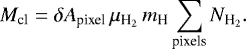
In the above equation, δApixel is the surface area of one pixel at the adopted distance (d = 400 pc),  is the mean molecular weight per H2 molecule, mH is the hydrogen atom mass, and the sum of column density values is over all of the pixels in the map. This approach yielded a total cloud mass of ~2.8 × 10⁴ M⊙.
In order to obtain the cumulative mass fraction of gas mass as a function of column density (Fig. 4 right), we repeated the above mass calculation for the pixels above a given column density. The dense molecular gas material represents only ~13% (~ 3.7 × 10³ M⊙) of the total cloud mass above a visual extinction AV ~ 7 mag. As in otherclouds, the low and intermediate column density regions at AV < 3–7 mag in the map of Fig. 2 (left) occupy most (>95%) of the surface area imaged with Herschel and account for most (~ 74−88%) of the cloud mass.
In agreement with the typical ratios AV, HGBS∕AV, ext≳0.5 found in Sect. 3.1 from comparing the HGBS column density map with extinction maps, we note that the total mass reported here for the Orion B clouds is a factor of ~ 1.8 lower than the total mass indicated by the extinction maps (~ 5 × 10⁴ M⊙).
 |
Fig. 4 Left: high-resolution |


3.4 Multiwavelength core extraction with getsources
Compact sources were extracted simultaneously from the PACS and SPIRE images with the getsources algorithm (Men’shchikov et al. 2012)2. A complete summary of the source extraction method can be found in Sect. 4.4 of Könyves et al. (2015), and full technical details are provided in Men’shchikov et al. (2012). Briefly, the extraction process consists of a detection and a measurement stage. At the detection stage, getsources analyzes fine spatial decompositions of all the observed wavebands over a wide range of scales. This decomposition filters out irrelevant spatial scales and improves source detectability, especially in crowded regions and for extended sources. The multi-wavelength design combines data over all wavebands and produces a wavelength-independent detection catalog. At the measurement stage, properties of detected sources are measured in the original observed images at each wavelength.
For the production of HGBS first-generation catalogs of starless and protostellar cores, two sets of dedicated getsources extractions are performed, optimized for the detection of dense cores and YSOs/protostars, respectively. In the first, “core” set of extractions, all of the Herschel data tracing column density are combined at the detection stage, to improve the detectability of dense cores. The detection image is thus combined from the 160, 250, 350, and 500 μm maps, together with the high-resolution column density image (see Sect. 3.1) used as an additional “wavelength”. The 160 μm component of the detection image is “temperature-corrected” to reduce the effects of strong, anisotropic temperature gradients present in parts of the observed fields (see Könyves et al. 2015, for details).
A second, “protostellar” set of getsources extractions is performed to trace the presence of self-luminous YSOs/protostars and discriminate between protostellar and starless cores. In this second set of extractions, the only Herschel data used at the detection stage are the PACS 70 μm data. This allows us to exploit the result that the level of point-like 70 μm emission traces the internal luminosity (and therefore the presence) of a protostar very well (e.g., Dunham et al. 2008).
At the measurement stage of both sets of extractions, source properties are measured at the detected positions of either dense cores or YSOs/protostars, using the observed, background-subtracted, and deblended images at all five Herschel wavelengths, plus the high-resolution column density map. The only difference from the procedure described in Könyves et al. (2015) is that, following improvements in the preparation of maps for source extraction, a new method of background flattening, called getimages (Men’shchikov 2017), was used before performing the protostellar set of getsources extractions. Tests have shown that this additional step drastically reduces the large number of spurious 70 μm sources in areas of bright, structured PDR (photodissociation region) emission around HII regions. Before extracting protostellar sources, getimages subtracts the large-scale background emission and equalizes the levels of small-scale background fluctuations in the images using a median-filtering approach.
3.5 Selection and classification of reliable core detections
3.5.1 Initial core selection
The criteria used to select reliable dense cores and YSOs from the raw source catalogs delivered by getsources are described in detail in Sect. 4.5 of Könyves et al. (2015).
First weselect candidate dense cores (starless and protostellar) from the “core” extractions using criteria based on several output parameters provided by getsources: detection significance, signal-to-noise ratio (S/N), and “goodness” parameter. Then, we select candidate YSOs from the second set of extractions based on their corresponding detection significance, S/N, flux density, goodness, and source size and elongation parameters.
Afterward, we cross-match the selected dense cores with the candidate YSOs/protostars and distinguish between starless cores and young (proto)stellar objects based on the absence or presence of compact 70 μm emission. YSOs must be detected as compact emission sources above the 5σ level at 70 μm, while starless cores must remain undetected in emission (or detected in absorption) at 70 μm (Könyves et al. 2010).
In addition to Aquila (Könyves et al. 2015), this whole method has been so far applied to studies of various regions of the HGBS: the Taurus L1495 cloud (Marsh et al. 2016), Corona Australis (Bresnahan et al. 2018), the Lupus complex (Benedettini et al. 2018), Perseus (Pezzuto et al. 2019), Ophiuchus (Ladjelate et al. 2019), the Cepheus Flare (Di Francesco et al., in prep.), further parts of Taurus (Kirk et al., in prep.), and the Orion A clouds (Polychroni et al., in prep.).
3.5.2 Post-selection checks
All of the candidate cores initially selected using the criteria defined in detail in Sect. 4.5 of Könyves et al. (2015) were subsequently run through an automated post-selection step. Given the large number (~ 2000) of compact sources detected with Herschel in the Orion B region, we tried to define automatic post-selection criteria based on source morphology in the SPIRE and PACS and column density images (see blow-up maps in Figs. A.1 and A.2), in order to bypass the need for detailed visual inspection. A final visual check of all candidate cores in the present catalog (Table A.1) was nevertheless performed. With our automated post-selection script described in detail in Appendix B, we revisited the location of each formerly selected core in all of the Herschel maps (including the column density plane) and performed a number of pixel value checks within and around the core’s FWHM contour to make sure that it corresponds to a true intensity peak or enhancement in the analyzed maps. This post-selection procedure allowed us to remove dubious sources from the final catalog of cores in Table A.1.
To eliminate extragalactic contaminants from our scientific discussion, we cross-matched all selected sources with the NASA Extragalactic Database3 (NED). We found matches within 6′′ for four classified external galaxies, which were removed from our scientific analysis. As Orion B lies toward the outer Galaxy and below the Galactic plane, we can expect several extragalactic contaminants in the low column density portions of the field, beyond the four sources listed in the NED database. Using Herschel’s SPIRE data from the HerMES extragalactic survey (Oliver et al. 2012), Oliver et al. (2010) determined that the surface number density of extragalactic sources at the level S250μm = 100 mJy is about 12.8 ± 3.5 deg−2. In the ~19 deg2 area observed with Herschel in Orion B, our catalog includes three candidate cores with 250 μm integrated flux densities below 100 mJy and 26 candidate cores with 250 μm integrated flux densities below 200 mJy, mostly in low background emission spots. Rougly 1/3 of these candidate cores with low flux densities at 250 μm have Unclassified Extragalactic Candidate matches within 6′′. These 26 tentative cores are listed in our observed core catalog (Table A.1), but excluded from the scientific analysis.
Likewise, we checked likely associations between the selected Herschel cores and objects in the SIMBAD database or the Spitzer database of Orion by Megeath et al. (2012). Any match is reported in the catalog of Table A.1. In particular, 30 associations with a Spitzer source were found using a 6′′ matching radius, where we used the same selection of YSOs from Megeath et al. (2012) as Shimajiri et al. (2017).
Overall, our getsources selection and classification procedure resulted in a final sample of 1844 dense cores in Orion B (not counting ~ 26 possible extragalactic contaminants), comprising 1768 starless cores and 76 protostellar cores (see Fig. 5). The observed properties of all these post-selected Herschel cores are given in the accompanying online catalog with a few example lines in Table A.1. The corresponding derived properties of the 1844 dense cores are provided in Table A.2.
3.6 Derived core properties
For derivingcore physical properties we used a SED fitting procedure similar to that described in Sect. 3.1 for the production of the column density map. The SED data points for the properties of each core were given by their integrated flux densities measured by getsources, and the data points were weighted by 1/ , where σerr is the flux measurement error estimated by getsources for each data point. The modified blackbody fits of the observed SEDs were obtained in IDL with the MPCURVEFIT routine (Markwardt 2009). These fits provided direct mass and line-of-sight-averaged dust temperature estimates for most of the selected cores. We derived core masses with the same dust opacity assumptions as in Sect. 3.1and a distance d = 400 pc for Orion B. The angular FWHM size estimates, measured by getsources at 18.2′′ resolution in the high-resolution column density map, were converted to a physical core radius. In our catalog (see Table A.2), we provide estimates for both the deconvolved and the observed radius of each core (estimated as the geometrical average between the major and minor FWHM sizes).
For each core, the peak (or central beam) column density, average column density, central-beam volume density, and the average volume density were then derived based on their mass and radius estimates (see Sect. 4.6. in Könyves et al. 2015). The column- and volume density distributions for the different population of cores are shown in Fig. 6. In Table A.2, all the above derived properties are provided for the whole sample of selected Herschel cores.
In order to assess the robustness of our SED fits for each source, we compared two successive runs of the fitting procedure with somewhat different weighting schemes. In the first run the getsources detection errors were used to weigh the SED points and the 70 μm data were included in the fit, while the more conservative measurement errors were used without fitting the 70 μm data points in the second run. The following criteria were applied for accepting the SED fits for a given source: (1) significant flux measurements exist in at least three Herschel bands, (2) the source has larger integrated flux density at 350 μm than at 500 μm, and (3) less than a factor of 2 difference is found between the core mass estimates from the two SED fits.
The starless core masses with rejected SED fit results from the above procedure were estimated directly from the measured integrated flux density at the longest significant wavelength. Optically thin dust emission was assumed at the median dust temperature that we found for starless cores with reliable SED fits. Such cores have more uncertain properties for which we assigned a “no SED fit” comment in Table A.2.
The accuracy of our core mass estimates is affected by two systematic effects: (1) uncertainties in the dust opacity law induce mass uncertainties of up to a factor ~1.5–2 (cf. Roy et al. 2014), (2) the SED fits only provide line-of-sight averaged dust temperatures. In reality, however, starless cores are externally heated objects, and they can show a significant drop in dust temperature toward their centers (e.g., Nielbock et al. 2012; Roy et al. 2014). The mass of a starless core may be underestimated in such a situation, as the average SED temperature may overestimate the mass-averaged dust temperature. For low column density cores, such as B68 (Roy et al. 2014), this effect is less than ~ 20%, but for high-density cores, with average column densities above ~1023 cm−2, it increases to up to a factor of ~2. Here, we did not attempt to use special techniques (cf. Roy et al. 2014; Marsh et al. 2014) to retrieve the intrinsic temperature structure and derive more accurate mass estimates.
The Monte–Carlo simulations that we used to estimate the completeness of the survey (see Sect. 3.8 below), however show that the SED masses of starless cores (in Table A.2) are likely underestimated by only ~ 25% on average compared to the intrinsic core masses. This is mainly because the SED dust temperatures slightly overestimate the intrinsic mass-averaged temperatures within starless cores. We have not corrected the column- and volume densities in Table A.2 and in Fig. 6 for this small effect.
We may also compare the results of the present core census with the SCUBA-2 findings of Kirk et al. (2016a), used in both Kirk et al. (2016b) and Parker (2018). Adopting a matching separation of < 6′′, we found 192 matches between HGBS starless cores and SCUBA-2 cores and 47 matches between HGBS protostellar cores and SCUBA-2 objects. The relatively low number of matches is the result of the significantly smaller area coverage of the SCUBA-2 data, the higher sensitivity and broader wavelength coverage of the Herschel data, and very different source-extraction techniques. As the assumptions about dust emissivity properties differ in the HGBS and SCUBA-2 studies, we re-derived two sets of mass estimates for the SCUBA-2 cores from the published 850 μm total fluxes: (1) the first set of mass estimates (MSCUBA-2, Td) was derived using the standard HGBS dust opacity law (see Sect. 3.1) and the dust temperatures estimated from Herschel SED fitting ( ); (2) the second set (MSCUBA-2, 20K) was derived using the same HGBS dust opacity law and a uniform dust temperature of 20 K for all cores (as assumed by Kirk et al. 2016a). The resulting comparison of core mass estimates is summarized in Fig. E.3, which plots the distributions of the ratios MSCUBA-2, Td∕MHGBS and MSCUBA-2, 20K∕MHGBS for all SCUBA-2–HGBS core matches, separately for starless and protostellar cores. In each panel of Fig. E.3, the corresponding median ratio is indicated by a red dashed line. Overall, a good correlation exists between the re-derived SCUBA-2 masses and the HGBS masses. The MSCUBA-2, Td mass estimates for the matched starless cores are typically only ~25% higher, and the MSCUBA-2, 20K estimates ~60% lower, than the MHGBS masses. The most likely reason for the relatively low MSCUBA-2, 20K∕MHGBS ratios is that the typical dust temperature of starless cores is significantly lower than 20 K, implying that MSCUBA-2, 20K typically underestimates the true mass of a starless core. For the 47 matched protostellar cores, the MSCUBA-2, 20K∕MHGBS ratio is close to 1 on average, indicating a very good agreement between the MSCUBA-2, 20K and MHGBS mass estimates, while the MSCUBA-2, Td masses are typically a factor of ~2 higher than the MHGBS masses. The latter trend most likely arises from the fact that the dust temperature
  , derived from our standard SED fitting between 160 and 500 μm, typically overestimates the “mass-averaged” temperature of a protostellar core. We stress, however, that
  is more reliable for starless cores and that protostellar cores are not the main focus of the present paper.
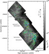 |
Fig. 5 High-resolution (~18″) column density map of Orion B, derived from SPIRE and PACS observations. The positions of the 1768 identified starless cores (green triangles), 490 robust prestellar cores (blue triangles), and 76 embedded protostellar cores (red symbols) are overplotted. The vast majority of the cores lie in high column density areas. The white declination line at Dec2000 = 1° 31′ 55″ marks the lower boundary of the northern region where cores may be associated with the Barnard’s Loop and at a more uncertain distance (d ~ 170–400 pc). See Sects. 1 and 3.5.2 for details. |
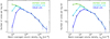 |
Fig. 6 Distributions of beam-averaged column densities (left) and beam-averaged volume densities (right) at resolution of SPIRE 500 μm observations for 1768 starless cores (green), 804 candidate prestellar cores (light blue), and 490 robust prestellar cores (dark blue curve) in Orion B. |
3.7 Selecting self-gravitating prestellar cores
The subset of starless cores which are self-gravitating are likely to evolve to protostars in the future and can be classified as prestellar cores (cf. Ward-Thompson et al. 2007). In the absence of spectroscopic observations for most of the Herschel cores, the self-gravitating status of a core can be assessed using the Bonnor–Ebert (BE) mass ratio αBE = MBE,crit∕Mobs, where Mobs is the core mass as derived from Herschel data and MBE,crit is the thermal value of the critical BE mass. The first criterion adopted here to select self-gravitating cores is αBE ≤ 2. This simplified approach, using the thermal BE mass and thus neglecting the nonthermal component of the velocity dispersion, is justified by observations of nearby cores in dense gas tracers (e.g., Myers 1983; Tafalla et al. 2002; André et al. 2007). These studies show that the thermal component dominates at least in the case of low-mass cores. The thermal BE mass (MBE) was estimated for each object from the deconvolved core radius (Rdeconv) that we measured in the high-resolution column density map (see Sect. 3.6) assuming 10 K as a typical internal core temperature4.
This selection of self-gravitating cores is illustrated in the mass versus size diagram of Fig. 7, where source positions can be used to distinguish between robust prestellar cores (filled blue triangles) and unbound starless cores (open green triangles).
In addition, a second, less restrictive selection of candidate prestellar cores (open light blue triangles in Fig. 7) was obtained by deriving an empirical lower envelope for self-gravitating objects in the mass versus size diagram, based on the Monte-Carlo simulations used in Sect. 3.8 to derive the completeness of the survey. The advantage of this less restrictive selection criterion, also employed by Könyves et al. (2015) in the Aquila cloud, is that it provides a larger, more complete sample of candidate prestellar cores (at the cost of including a larger fraction of misclassified unbound cores).
Here, the resulting final number of robust prestellar cores based on the first criterion (αBE ≤ 2) was 490, and the number of candidate prestellar cores based on the empirical criterion was 804, out of a grand total of 1768 starless cores in the entire Orion B field. The spatial distribution of all starless cores and robust prestellar cores is plotted in Fig. 5. We note that all of the robust prestellar cores belong to the wider sample of candidate prestellar cores.
These two samples of prestellar cores reflect the uncertainties in the classification of gravitationally bound/unbound objects, which are fairly large for unresolved or marginally-resolved cores, as the intrinsic core radius (and therefore the intrinsic BE mass) is more uncertain for such cores. In the following discussion (Sect. 4) below, we consider both samples of prestellar cores. The 314 candidate prestellar cores which are not robust are clearly marked with a “tentative bound” comment in Table A.2.
In the northern region around L1622, which may be associated with Barnard’s Loop, there are 179 starless cores (~10% of the whole sample of starless cores), including 67 candidate prestellar cores (or ~8% of all candidate prestellar cores), 41 robust prestellar cores (~8%), and 15 protostellar cores (~20% of all protostellar cores). As mentioned in Sect. 1, these cores are at a more uncertain distance. By default and for simplicity, these northern objects are assumed to be at the same distance of 400 pc as the rest of the cores (cf. Ochsendorf et al. 2015). The cores lying north of the declination line Dec2000 = 1° 31′ 55″ in Fig. 5 are nevertheless marked with an “N region” comment in the catalogs available at the CDS (Tables A.1 and A.2).
In the mass versus size diagram of Fig. 7 for the entire population of starless cores, there is a spread of deconvolved sizes ( ) between ~ 0.01 pc and ~ 0.1 pc and a range of core masses between ~0.02 M⊙ and ~ 20 M⊙. The fraction of self-gravitating starless objects is ~28% or ~45% considering the samples of robust or candidate prestellar cores, respectively. Most of the unbound starless cores identified with Herschel in Orion B are located in the same area of the mass vs. size diagram as typical CO clumps (marked by the yellow band in Fig. 7), which are known to be mostly unbound structures (e.g., Elmegreen & Falgarone 1996; Kramer et al. 1998). It can also be seen in Fig. 7 that self-gravitating prestellar cores are typically more than an order of magnitude denser than unbound CO clumps.
Finally, we note that the distributions of beam-averaged column densities and volume densities for starless cores, candidate prestellar cores, and robust prestellar cores all merge at high (column) densities in Fig. 6, suggesting that all Herschel starless cores with 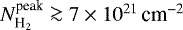 or
or 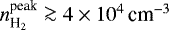 are dense enough and sufficiently strongly centrally concentrated to be self-gravitating and prestellar in nature.
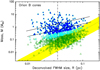 |
Fig. 7 Mass versus size diagram for all 1768 starless cores (triangles) identified with Herschel in Orion B, including the 804 candidate prestellar cores (light or dark blue triangles) and 490 robust prestellar cores (filled triangles in dark blue). The core FWHM sizes were measured with getsources in the high-resolution column density map (Fig. 2 left) and deconvolved from an 18.2′′ (HPBW) Gaussian beam. The corresponding physical |

3.8 Completeness of the prestellar core survey
Following the Monte–Carlo procedure used by Könyves et al. (2015) to estimate the completeness limit of the HGBS prestellar core census in the Aquila cloud, we performed similar simulations in Orion B. A population of 711 model Bonnor–Ebert-like cores were inserted in clean-background images at the Herschel wavelengths, from which we also derived a synthetic column density plane as described in Sect. 3.1. Then, core extractions were performed on the resulting synthetic images with getsources in the same way as for the observed data (see Sect. 3.4). The results of these simulations suggest that our sample of candidate prestellar cores in Orion B is > 80% complete above a true core mass of ~0.5 M⊙ (cf. Fig. 8), which translates to ~0.4 M⊙ in observed core mass. Indeed, the observed masses of starless cores tend to be underestimated by ~25% due to their internal temperature gradient (see Fig. C.1–left and Appendix C for further details).
In Appendix B of Könyves et al. (2015) it was shown that the completeness level of a census of prestellar cores such as the present survey is background dependent, namely that the completeness level decreases as background cloud column density and cirrus noise increase. A similar model adapted to the case of Orion B quantifies this trend (see Fig. C.4) and shows that the global completeness of the present census of prestellar cores is consistent with that inferred from the Monte–Carlo simulations (see Fig. 8 and Appendix C).
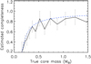 |
Fig. 8 Completeness curve of candidate prestellar cores as function of true core mass (solid line), which was estimated from Monte–Carlo simulations (see Sect. 3.8). For comparison, the global completeness curve of the model introduced at the end of Appendix C is shown by the dashed blue line. |
4 Discussion
4.1 Spatial distribution of dense cores
4.1.1 Connection between dense cores and filaments
As already pointed out in earlier HGBS papers (e.g., André et al. 2010; Könyves et al. 2015; Marsh et al. 2016; Bresnahan et al. 2018), there is a very close correspondence between the spatial distribution of compact dense cores and the networks of filaments identified in the Herschel column density maps of the Gould Belt regions. Furthermore, prestellar cores and embedded protostars are preferentially found within the densest filaments with transcritical or supercritical masses per unit length (i.e., 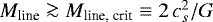 ) (e.g., André et al. 2010, 2014).
The two panels of Fig. 9 provide close-up views of two subfields of Orion B, where the projected locations of robust prestellar cores are overlaid on the filament masks (shown up to 100′′ transverse angular scales) extracted with getfilaments (see Sect. 3.2). More than 80% of the robust prestellar cores are found inside this filament sample in the whole Orion B region. The connection between cores and filaments can be quantified in more detail based on the census of cores presented in Sects. 3.4, 3.5, and 3.7 and the census of filaments described in Sect. 3.2. The locations of extracted cores were correlated with various filament samples to illustrate the robustness of this connection. We consider three of these filament samples, also displayed in Fig. 3:
-
getfilaments mask images including transverse angular scales up to 50′′ or 100′′, which correspond to transverse physical scales up to ~0.1 pc or ~0.2 pc at d = 400 pc. Such 100′′ mask images are shown in grayscale in, for example, Fig. 3.
-
Maps of robust filament crests extracted with the DisPerSE algorithm and cleaned with the criteria described in Sect. 3.2 (thick blue skeletons overplotted in Fig. 3). Corresponding mask images were prepared from the 1-pixel-wide crests using Gaussian smoothing kernels with three different FWHM widths: 0.05 pc, 0.1 pc, and 0.2 pc.
-
Maps of raw filament crests extracted with the DisPerSE algorithm, prior to cleaning and post-selection (see Sect. 3.2). In Fig. 3, the combination of blue and cyan filament crests together make up the DisPerSE raw sample. As for DisPerSE robust crests, mask images were prepared using three Gaussian smoothing kernels with FWHMs of 0.05 pc, 0.1 pc, and 0.2 pc.
Table 2 reports the fractions of cores lying within the footprints of each of the above-mentioned filament samples, assuming that the intrinsic inner width of each filament is within a factor of 2 of the typical 0.1 pc value found by Arzoumanian et al. (2011, 2019) in nearby clouds, including Orion B.
We also derived the distribution of core separations to the nearest filament crests using various core samples (starless, candidate and robust prestellar) and the crests of both the robust and the raw sample of DisPerSE filaments. The results shown in Fig. 10 were obtained with the raw (uncleaned) sample of DisPerSE filaments. The median separation to the nearest filament is 0.006 pc for the robust (dark blue histogram) and candidate (light blue) prestellar core samples, and 0.007 pc for the starless core sample (green).
The fraction of cores within the nominal filament width (0.1 pc) of the raw DisPerSE sample, marked by the red vertical line in Fig. 10, is also presented in Table 2. Based on the numbers given in Table 2, we confirm that a high fraction of prestellar cores are closely associated with filaments in Orion B, as already observed in Aquila (Könyves et al. 2015), Taurus L1495 (Marsh et al. 2016), and Corona Australis (Bresnahan et al. 2018), for example.
The tight connection between cores and filaments is found independently of the detailed algorithm employed to trace filamentary structures (see Table 2). In particular, while one may think that the association between cores and filaments is partly an artificial consequence of the way DisPerSE constructs filament crests (by joining saddle points to local maxima), we stress that the same connection is seen when using getfilaments to determine filament footprints completely independently of column density maxima (see Sect. 3.2).
When the DisPerSE raw samples of filaments are considered (which are the most complete samples of elongated structures used in Table 2), the distributions show that most (≳90%) starless or prestellar dense cores lie very close to identified filamentary structures. This suggests that the earliest phases of star formation are necessarily embedded in elongated structures (of any density), which may provide an optimal basis for cores to gain mass from their immediate environment. Such an increase in the number of cores residing in filaments when considering a more complete filament sample is also found in the Aquila cloud.
4.1.2 Nearest neighbor core separation
The distributions of nearest-neighbor core separations are plotted in Fig. 11 for all starless cores (green histogram) and both candidate and robust prestellar cores (light and dark blue histograms, respectively). When deriving these distributions, each set of dense cores was analyzed separately, and only separations between cores of the same category were considered. The median nearest-neighbor core separation is similar, ~0.14 pc for all three samples. Interestingly, the histograms show steep rises (at ~0.07 pc) and falls (at ~0.2 pc), which bracket the characteristic ~0.1 pc inner width of nearby filaments (Arzoumanian et al. 2019).
Similar distributions of nearest-neighbor core separations are found for the samples of Aquila cores from Könyves et al. (2015), for which the median nearest-neighbor core separation is 0.09 pc, and the most significantly rising and falling histogram bins are at separations of ~0.06 and ~0.1 pc, respectively.
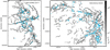 |
Fig. 9 Spatial distributions of robust prestellar cores (blue symbols) overplotted on the filament networks (gray background images) traced with getfilaments in NGC 2068 and 2071 (left), and NGC 2023 and 2024 (right). Transverse angular scales up to 100′′ across the filament footprints are shown here, corresponding to ~0.2 pc at d = 400 pc. In both panels, the color scale displayed within the filament mask corresponds to column density values in the original column density map (Fig. 2 left). See Fig. E.2 (right) for a similar view in the case of L1622. |
Fractions of cores associated with filaments in Orion B.
4.2 Mass segregation of prestellar cores
Investigating how dense cores of different masses are spatially distributed (and possibly segregated) is of vital interest for understanding the formation and early dynamical evolution of embedded protostellar clusters.
Figure 12 shows the median mass of candidate prestellar cores as a function of ambient column density in the parentcloud. The upper panel displays the median core mass as observed in each column density bin before any correction for incompleteness effects, while the lower panel displays median core masses corrected for incompleteness. The incompleteness correction was achieved as follows, using the model completeness curves presented in Appendix C as a function of background column density (see Fig. C.4). In each bin of background column densities as estimated by getsources, each observed core mass was weighted by the inverse of the model completeness fraction before computing the weighted median mass and interquartile range for that bin. It can be seen in Fig. 12 that both the median prestellar core mass and the dispersion in core masses increase with background column density. Moreover, this increase in core mass and mass spread is robust and not dominated by incompleteness effects which make low-mass cores somewhat more difficult to detect at higher background column densities (see lower panel of Fig. 12).
Taking differential incompleteness effects into account (cf. Fig. C.4), this suggests that both higher- and lower-mass prestellar cores may form in higher density clumps and filaments, a trend also seen in the Aquila cloud (cf. André et al. 2017). A simple interpretation of this trend is that the effective Jeans mass increases roughly linearly with background column density, because the velocity dispersion is observed to scale roughly as the square root of the column density (see, e.g., Heyer et al. 2009; Arzoumanian et al. 2013), while the thermal Jeans mass decreases roughly linearly with background column density (see Eq. (1) of André et al. 2019).
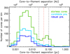 |
Fig. 10 Distribution of separations between dense cores and the nearest filament crests in the DisPerSE raw sample of filaments. The green histogram is for all 1768 starless cores, the light blue histogram for the 804 candidate prestellar cores, and the dark blue histogram for the 490 robust prestellar cores. The vertical lines mark the half widths (i.e., on either side of the filament crests) of a 0.1 pc-wide (red), 0.5 × 0.1 pc-wide (inner black), and a 2 × 0.1 pc-wide (outer black) filament. |
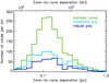 |
Fig. 11 Distribution of nearest-neighbor core separations in Orion B. The green, light-, and dark blue histograms show the distributions of nearest-neighbor separations for starless cores (either bound or unbound), candidate prestellar cores, and robust prestellar cores, respectively. In each case, only the separations between cores of the same category were considered. The median core separation is ~ 0.14 pc for all three core samples. |
4.3 Prestellar core mass function
The core mass functions derived for the samples of 1768 starless cores, 804 candidate prestellar cores, and 490 robust prestellar cores identified in the whole Orion B cloud are shown as differential mass distributions in Fig. 13 (green, light blue, and dark blue histograms, respectively). We note that all three distributions merge at high masses, which simply reflects the fact that all of the starless cores identified above ~ 1 M⊙ are dense and massive enough to be self-gravitating, hence prestellar in nature.
The high-mass end of the prestellar CMF above 2 M⊙ is well fit by a power-law mass function, ΔN/Δ logM ∝ M−1.27 ± 0.24 (see Fig. 13), which is consistent with the Salpeter power-law IMF (ΔN/Δ logM⋆ ∝  in the same format – Salpeter 1955). The black solid line in Fig. 13 is a least-squares fit. A non-parametric Kolmogorov-Smirnov (K-S) test (see, e.g. Press et al. 1992) confirms that the CMF above 2 M⊙ is consistent with a power-law mass function, ΔN/ΔlogM ∝ M−1.33 ± 0.13, at a significance level of 95%.
The observed peak of the prestellar CMF at ~ 0.4–0.5 M⊙ is similar to that seen in the Aquila region (cf. Fig. 16 of Könyves et al. 2015) but is here extremely close to the estimated 80% completeness limit of 0.4 M⊙ in observed core mass (cf. Sect. 3.8 and Appendix C). It may therefore not be significant.
In order to further test the mass segregation result discussed in Sect. 4.2 above, Fig. 14 compares the CMF of candidate prestellar cores observed at low and intermediate background column densities ( , purple histogram) with that observed at high background column densities (
 , magenta histogram). It can be seen that the prestellar CMF observed at high background AV values peaks at an order of magnitude higher mass than the prestellar CMF observed at low and intermediate background AV values, that is, ~3.8 M⊙ versus ~0.4 M⊙, respectively.Indeed, the majority of prestellar cores found at low and intermediate
  have significantly lower masses than the majority of prestellar cores found at high
  , which corresponds to the findings of Sect. 4.2 (see Fig. 12). The split in background visual extinction at
  and
and  was somewhat arbitrary, but similar –albeit less significant– results are obtained with other low and high background extinction limits.
Interestingly, a similar difference between the prestellar CMFs observed at high and low background AV values is also seen in the Aquila cloud (André et al. 2017), and a related result was also found in Orion A, where Polychroni et al. (2013) reported two distinct mass distributions for cores “on” and “off” prominent filaments, that is, at high and low background AV, respectively.We also note that, based on recent ALMA observations, Shimajiri et al. (2019) found a CMF peaking at ~ 10 M⊙ in the very dense, highly supercritical filament of NGC 6334 (with Mline ≈ 500–1000 M⊙∕pc ≫ Mline, crit, corresponding to  ), which is again consistent with the same trend.
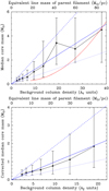 |
Fig. 12 Top: median prestellar core mass versus background column density (black triangles). The error bars correspond to the inter-quartile range in observed masses for each bin of background column density. The solid, dashed and dotted blue lines are linear fits to the observed median, upper-quartile, and lower-quartile masses as function of background column density, respectively. The red curve shows how the mass at the 50% completeness level varies with background column density according to the model completeness curves of Appendix C (see Fig. C.4). The upper x-axis provides an approximate mass-per-unit-length scale, assuming the local backgroundaround each core is dominated by the contribution of a parent filament with a characteristic width Wfil = 0.1 pc (see end of Sect. 4.5). Bottom: same as upper panel after correcting the distribution of observed core masses for incompleteness effects before estimating the median core mass and inter-quartile range in each column density bin (see Sect. 4.2). Both the median prestellar core mass and the dispersion in core masses increase roughly linearly with background column density. |
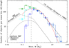 |
Fig. 13 Differential core mass function (ΔN/ΔlogM) of the 1768starless cores (green histogram), 804 candidate prestellar cores (light blue histogram), and 490 robust
prestellar cores (dark blue histogram) identified with Herschel in the whole Orion B field. The error bars correspond to
|

 |
Fig. 14 Comparison of the differential CMF (ΔN/ΔlogM) derived for the 558 candidate prestellar cores lying in areas of low background column density ( |


4.4 Massbudget in the cloud
Using our Herschel census of prestellar cores and filaments, we can derive a detailed mass budget for the Orion B cloud. In the intermediate column density regions ( ), a large fraction, ~60%, of the gas mass is in the form of filaments but only ~3 − 5% of the cloud mass is in the form of prestellar cores. In higher column density regions (
 ), a similarly high fraction of the cloud mass is in the form of filaments and a fraction fpre ~ 22% of the mass is in the form of prestellar cores.
In an attempt to quantify further the relative contributions of cores and filaments to the cloud material as a function of column density, we compare in Fig. 15 the column density PDFs observed for the cloud before any component subtraction (blue histogram, identical to the PDF shown in Fig. 4 left), after subtraction of dense cores (red solid line), and after subtraction of both dense cores and filaments (black solid line). To generate this plot, we used getsources to create a column density map of the cloud after subtracting the contribution of all compact cores, and getfilaments to construct another column density map after also subtracting the contribution of filaments. Although there are admittedly rather large uncertainties involved in this two-step subtraction process, the result clearly suggests that filaments dominate the mass budget in Orion B throughout the whole column density range. In the Lupus region, Benedettini et al. (2015) also found that the power-law tail of their PDF is dominated by filaments.
4.5 Column density transition toward prestellar core formation
The existence of thresholds for star formation have been suspected for a long time, based on the results of ground-based millimeter and submillimeter surveys for cores in, for instance, the Taurus, Ophiuchus, and Perseus clouds (e.g., Onishi et al. 1998; Johnstone et al. 2004; Hatchell et al. 2005). Following these early claims, the HGBS results in Aquila and Taurus provided a much stronger case for a column density threshold for prestellar core formation (André et al. 2010; Könyves et al. 2015; Marsh et al. 2016) thanks to the excellent column density sensitivity and high spatial dynamic range of the Herschel imaging data, making it possible to probe prestellar cores and the parent background cloud simultaneously. The Herschel results on the characteristic inner width of filaments (Arzoumanian et al. 2011, 2019) and the tight connection observed between cores and filaments (cf. Sect. 4.1.1) also led to a simple interpretation of this threshold in terms of the critical mass per unit length of nearly isothermal cylinder-like filaments (André et al. 2014).
To investigate whether a column density threshold for core formation is present in Orion B, and following the study of Könyves et al. (2015) in Aquila, we plot in Fig. 16 the differential prestellar core formation efficiency CFE_obs(AV) = ΔMcores(AV)∕ΔMcloud(AV) as a function of the background cloud column density in the Orion B complex. This was obtained by dividing the mass ΔMcores(AV) of the candidate prestellar cores identified with Herschel in a given bin of background column densities (expressed in AV units) by the total cloud mass ΔMcloud(AV) in the same bin. It can be seen in Fig. 16 that CFE_obs(AV) exhibits a steep rise in the vicinity of  and resembles a smooth step function, fairly similar to that observed in the Aquila cloud (see Fig. 12 of Könyves et al. 2015). The Herschel observations indicate a sharp transition between a regime of very low CFEobs at
  and a regime where CFEobs(AV) is an order of magnitude higher and fluctuates around a roughly constant value of ~ 15–20%. The combination of this sharp transition with the column density PDF of Fig. 4 implies that, at least in terms of core mass, most prestellar core formation occurs just above
  (see top panel of Fig. 17). Based on Figs. 16 and 17 (top panel), we argue for the presence of a true physical “threshold” for the formation of prestellar cores in Orion B around a fiducial value
  , which we interpret here as well as resulting from the mass-per-unit-length threshold above which molecular filaments become gravitationally unstable. It should be stressed, however,
  is only a fiducial value for this threshold, which for various reasons should rather be viewed as a smooth transition (see discussion in André et al. 2014). We also note some environmental variations in the details of this transition between Orion B and Aquila. In Orion B, the raw number of prestellar cores per column density bin peaks at
  (see bottom panel of Fig. 17) or at most at
  –6 if we take into account a correction factor AV, HGBS∕AV, ext ~ 0.5–0.6 between the
  values derived from the HGBS column density map and those derived from near-infrared extinction maps in the range AV = 3−7 mag (see Sect. 3.1). In Aquila, the raw number of prestellar cores peaks at a significantly higher background column density
  (see Fig. 11a of Könyves et al. 2015). Despite this difference, the shapes of the prestellar core formation efficiency as a function of background AV, CFE_obs(AV), are remarkably similar in the two clouds (compare Fig. 16 here with Fig. 12 of Könyves et al. 2015).
Core formation efficiency is discussed as a function of background column density or  here, as column density is the most directly observable quantity, but we can also provide a rough conversion in terms of background volume density and mass per unit length. In the 0.1-pc filament paradigm of core formation (André et al. 2014), the local background is dominated by the parent filament of each core and there is a direct correspondence between the average values of the surface density
  , volume density
  , and line mass Mline of the parent filament. For a cylindrical parent filament of width Wfil, one has: ⟨Σfil⟩ = Mline∕Wfil and
  . In particular, adopting a uniform filament width Wfil = 0.1 pc, the fiducial column density threshold at
  corresponds to a threshold line mass Mline, th ~ 15 M⊙ pc−1, very close to the thermal value of the critical mass per unit length Mline, crit ~ 16 M⊙∕pc for T ~ 10 K gas filaments (Ostriker 1964; Inutsuka & Miyama 1997), and to a threshold volume density
  . Alternatively, under the extreme assumption that the background cloud structure is completely isotropic, one can derive another conversion between column density and typical volume density (cf. Fig. A.1d of Bron et al. 2018), which leads to a significantly lower value of only ~103 cm−3 for the threshold volume density. Obviously, only an order-of-magnitude estimate of the threshold volume density can be derived. Because the Herschel data indicate that the local background around each core is highly anisotropic (e.g., filamentary), we nevertheless tend to favor our higher estimate of the threshold volume density (i.e., ~ 3 × 104 cm−3).
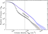 |
Fig. 15 Comparison of the global column density PDF in Orion B (blue histogram) to the column density PDF measured after subtraction of dense cores (red solid line) and the PDF measured after subtraction of both dense cores and filaments (black solid line with statistical error bars). The blue histogram is identical to that shown in Fig. 4 (left). The vertical dashed line marks the approximate separation between low-to-intermediate and high column density values at
|

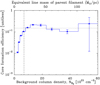 |
Fig. 16 Differential core formation efficiency (CFE) as function of ambient cloud column density expressed in AV units (blue histogram with error bars), obtained by dividing the mass in the form of candidate prestellar cores in a given column density bin by the cloud mass observed in the same column density bin. The upper x-axis provides an approximate mass-per-unit-length scale, assuming the local background around each core is dominated by the contribution of a parent filament with a characteristic width
Wfil = 0.1 pc (see end of Sect. 4.5). The vertical dashed line marks the fiducial threshold at
|

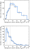 |
Fig. 17 Top: total mass in form of prestellar cores as function of ambient cloud column density in Orion B (blue histogram). Bottom: distribution of background column densities for the 490 robust prestellar cores (blue histogram). The vertical dashed lines mark
|

4.6 Lifetime of prestellar cores in Orion B
As our Herschel survey provides an essentially complete census of prestellar cores in the Orion B clouds, the core statistics can be used to set constraints on the typical lifetime of prestellar cores and the timescale of the core formation process. We may derive a rough lifetime by comparing the number of prestellar cores found here with Herschel to the number of Class II YSOs detected in the mid-IR by Spitzer in the same region. The same approach was first used by Beichman et al. (1986) based on IRAS data. Our findings will hold, assuming that (1) all prestellar cores will evolve into YSOs in the future, and (2) star formation proceeds at a roughly constant rate, at least when averaged over the entire Orion B cloud complex.
The three HGBS tiles imaged with Herschel around NGC 2023 and 2024, NGC 2068 and 2071, and L1622 (see, e.g., Fig. 2) were also observed by IRAC as part of the Spitzer Orion survey (Megeath et al. 2012) and thus provide a common field where Herschel and Spitzer source counts can be directly compared. The various numbers of dense cores and YSOs identified bythe two surveys in this common field are as follows:
-
Herschel starless cores: 1032; above the mass completeness limit of 0.4 M⊙: 338
-
Herschel candidate prestellar cores: 538; above 0.4 M⊙: 333
-
Herschel robust prestellar cores: 361; above 0.4 M⊙: 312
-
Spitzer Class II YSOs: 312; corrected for incompleteness: 427
-
Spitzer entire sample of Class 0/I–flat spectrum–Class II YSOs: 428; corrected for incompleteness: 586.
For our lifetime estimates, we used the numbers of Spitzer sources corrected for incompleteness with the help of Chandra data and other techniques as described in detail in Megeath et al. (2016). In practice, the corrected numbers of Spitzer sources were derived by multiplying the uncorrected number counts by a factor of 1.37, based on Table 1 of Megeath et al. (2016).
If we adopt a reference lifetime of 2 Myr for Class II YSOs (Evans et al. 2009), the comparison between Herschel and Spitzer source counts leads to lifetimes ranging from 2 × 312∕586 ≈ 1.1 Myr to 2 × 538∕427 ≈ 2.5 Myr for the prestellar core phase, depending on whether we consider only robust prestellar cores above our mass completeness limit of 0.4 M⊙ or all candidate prestellar cores, and all Spitzer YSOs up to Class II or only YSOs nominally classified as Class IIs. Our best estimate of the prestellar core lifetime in Orion B is thus 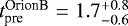 Myr, derived from the ratio 361/427 of the total number of Herschel prestellar cores to the number of Spitzer Class II YSOs corrected for incompleteness. This is slightly longer than, but consistent within errors with, the prestellar lifetime estimate derived by Könyves et al. (2015) in the Aquila cloud,
  Myr.
Myr.
As a result of non-uniform incompleteness effects between the Spitzer and the Herschel sample, the uncertainties in these lifetimes are admittedly rather large (at least a factor of ~ 2). Additional sources of errors possibly affecting the above lifetime estimate are: (1) Megeath et al. (2012) used infrared spectral index values uncorrected for extinction (in Aquila, the compared Spitzer sources had been dereddened), (2) the classification of cores and YSOs is somewhat uncertain, and (3) the two initial assumptions mentioned above (i.e., prestellar nature of the cores and steady state) may not entirely hold.
5 Summary and conclusions
Using SPIRE and PACS parallel-mode data from the Herschel Gould Belt survey, we obtained an extensive census of dense cores in the Orion B star-forming region. We analyzed both the physical properties of the cores and the connection with interstellar filaments. Our main results and conclusions can be summarized as follows:
- 1.
As in other HGBS clouds, the high-resolution (~18′′ or ~ 0.03 pc) Herschel column density map of Orion B shows a highly filamentary distribution of matter and the column density PDF features a prominent power-law tail above AV ~ 3 mag.
- 2.
Based on multi-scale, multi-wavelength core extraction with the getsources algorithm we identified 1768 starless dense cores, 804 candidate prestellar cores, 490 robust prestellar cores, and 76 protostellar cores in the ~19 deg2 field thatwas imaged with both SPIRE and PACS at five wavelengths between 70 μm and 500 μm. The ~80% mass completeness level for candidate prestellar cores was estimated to be at an observed core mass of ~0.4 M⊙. The candidate prestellar cores have an estimated median mass ~0.5 M⊙, a mediandeconvolved FWHM diameter ~0.03 pc, a medianaverage column density ~4 × 1021 cm−2, and a median average volume density ~3 × 104 cm−3.
- 3.
The identified dense cores are closely associated with filamentary structures. A very high fraction of prestellar cores (60–90%) were found within the 0.1 pc inner portion of the filaments extracted with both DisPerSE and getfilaments. Considering the deep raw sample of filaments extracted with DisPerSE, we find that almost all dense cores (>90%) lie within – stronger or fainter – elongated filamentary structures. Filaments may provide a more optimal environment for the growth of prestellar cores than spheroidal clumps.
- 4.
The most massive prestellar cores in our sample (with masses between M ~ 2 M⊙ and ~10 M⊙) tend to be spatially segregated in the highest column density portions of the Orion B cloud, at equivalent visual extinctions
 –30. In particular, the distribution of median prestellar core mass as a function of background column density (Fig. 12) shows that both the median core mass and the dispersion in core masses increase roughly linearly with background column density. This suggests that the prestellar core mass function (CMF) may not be strictly universal but may depend on the local column density in the ambient cloud. This also suggests that intermediate-mass and high-mass protostars may form only (or at least preferentially) in the dense inner portions of molecular clouds, supporting the notion of primordial mass segregation in stellar protoclusters.
 - 5.
The global differential CMF derived for the whole sample of 804 candidate prestellar cores (or 490 robust prestellar cores) peaks at ~0.5 M⊙ (in ΔN/ΔlogM format), which is just above the estimated 80% completeness limit of ~0.4 M⊙ in Orion B. The best power-law fit to the high-mass end of the prestellar CMF has a slope of –1.27 ± 0.24, compared to the Salpeter slope of − 1.35 (Fig. 13).
- 6.
Splitting the global sample of Orion B prestellar cores in a subsample of cores observed at high background column densities (
 ) and a subsample of cores observed at low and intermediate background column densities (
 ), we found that the CMF of the high-AV
subsample peaks at an order of magnitude higher mass (~3.8 M⊙) than the lower AV
subsample (~0.4 M⊙) (Fig. 14). This result, which cannot be explained by differential incompleteness effects, further illustrates the presence of significant mass segregation in the prestellar core population of the cloud.
), we found that the CMF of the high-AV
subsample peaks at an order of magnitude higher mass (~3.8 M⊙) than the lower AV
subsample (~0.4 M⊙) (Fig. 14). This result, which cannot be explained by differential incompleteness effects, further illustrates the presence of significant mass segregation in the prestellar core population of the cloud. - 7.
The Herschel data in Orion B confirm the presence of a column density transition around
 , for the formation of prestellar cores (Fig. 16). Coupled to the close connection observed between cores and filaments (point 3), this is consistent with the view that dense filamentary structures with line masses near or above the thermal value of the critical mass per unit length of isothermal cylinders provide the most favorable local environment for prestellar cores to grow within molecular clouds.
 - 8.
The typical lifetime of Herschel prestellar cores in Orion B was estimated to be
 Myr, which is consistent within error bars with the prestellar core lifetime
  Myr derived by Könyves et al. (2015) in the Aquila cloud.
Acknowledgements
SPIRE has been developed by a consortium of institutes led by Cardiff Univ. (UK) and including: Univ. Lethbridge (Canada); NAOC (China); CEA, LAM (France); IFSI, Univ. Padua (Italy); IAC (Spain); Stockholm Observatory(Sweden); Imperial College London, RAL, UCL-MSSL, UKATC, Univ. Sussex (UK); and Caltech, JPL, NHSC, Univ. Colorado (USA). This development has been supported by national funding agencies: CSA (Canada); NAOC (China); CEA, CNES, CNRS (France); ASI (Italy); MCINN (Spain); SNSB (Sweden); STFC, UKSA (UK); and NASA (USA). PACS has been developed by a consortium of institutes led by MPE (Germany) and including UVIE (Austria); KUL, CSL, IMEC (Belgium); CEA, OAMP (France); MPIA (Germany); IFSI, OAP/AOT, OAA/CAISMI, LENS, SISSA (Italy); IAC (Spain). This development has been supported by the funding agencies BMVIT (Austria), ESA-PRODEX (Belgium), CEA/CNES (France), DLR (Germany), ASI (Italy), and CICT/MCT (Spain). V.K. would like to thank Richard Allison, and Richard Parker for their help and discussions on mass segregation with the MST method. This work has received support from the European Research Council under the European Union’s Seventh Framework Programme (ERC Advanced Grant Agreements no. 291294 – ORISTARS – and no. 267934 – MISTIC) and from the French National Research Agency (Grant no. ANR–11–BS56–0010 – STARFICH). D.A. acknowledges support by FCT/MCTES through national funds (PIDDAC) by the grant UID/FIS/04434/2019. N.S. and S.B. acknowledge support by the French ANR and the German DFG through the project GENESIS (ANR–16–CE92–0035–01/DFG1591/2–1). G.J.W. gratefully acknowledges support from The Leverhulme Trust. We also acknowledgesupport from the French national programs of CNRS/INSU on stellar and ISM physics (PNPS and PCMI). This research hasmade use of the SIMBAD database, operated at CDS, Strasbourg (France), and of the NASA/IPAC Extragalactic Database (NED), operated by the Jet Propulsion Laboratory, California Institute of Technology, under contract with the National Aeronautics and Space Administration.
Appendix A Catalog of dense cores identified with Herschel in the Orion B cloud complex
With our Herschel SPIRE and PACS parallel-mode imaging survey of the Orion B cloud complex, we identified a total of 1844 dense cores, including 1768 starless cores and 76 protostellar cores. The master catalog listing the observed properties of all of these Herschel cores is available in Table A.1. A template of this online catalog is provided below to illustrate its form and content.
The derived properties (physical radius, mass, SED dust temperature, peak column density at the resolution of the 500 μm data, average column density, peak volume density, and average density) are given in Table A.2 for each core. A portion of this online table is also provided below.
The end of the catalog of observed core properties also includes 26 additional tentative cores which are possible extragalactic contaminants (see Sect. 3.5.2). The derived properties of these objects are not provided in Table A.2.
 |
Fig. A.1 Example blow-up Herschel images at 70–160–250–350–500 μm and high-resolution column density map for a (bound) prestellar core. Ellipses represent the estimated major andminor FWHM sizes of the core at each wavelength; they are shown as solid or dashed curves depending on whether the core is significantly detected or not, respectively, at a particular wavelength. See Table A.2 for the physical radius of the core and other derived properties. An angular scale of 30′′ (~ 0.058 pc at d = 400 pc) is shown at the bottom right. North is up, east is left. Similar image cutouts are provided online for all selected starless cores. |
 |
Fig. A.2 Same as Fig. A.1 for a protostellar core. See Table A.2 for its derived properties. Similar image cutouts are provided online for all selected protostellar cores. |
Catalog of dense cores identified in HGBS maps of Orion B (template, full catalog only provided at the CDS).
Derived properties of dense cores identified in HGBS maps of Orion B (template, full table only provided at the CDS).
Appendix B Automated post-selection of reliable core candidates
The getsources source extraction algorithm (Men’shchikov et al. 2012), which analyzes fine spatial decompositions of the original images across a wide range of scales and at all observed wavebands, is a powerful technique to extract most candidate dense cores in spatially-varying backgrounds. At the same time, however, this technique tends to extract irregularities in the emission maps used for detection which must be discarded by the user at the post-selection stage, that is after the initial selection criteria described in Sect. 3.5.1 have been automatically applied.
The criteria of Sect. 3.5.1 are applied to the raw output catalog from getsources. At this stage, the properties of candidate cores are derived directly from getsources measurements without going back to the observed maps themselves. After the initial selection steps, there may still be a significant number of spurious sources in the selected core list which do not correspond to real emission peaks or do not appear like genuine cores in the maps. These spurious sources can only be eliminated by revisiting their locations in the Herschel maps, which is done here with a separate automated script. This “post-selection” script is run on the same input observed maps with 3′′ pixels as used for the getsources extractions.
 |
Fig. B.1 Close-up view of a post-selected prestellar core at 500 μm (shown in Fig. A.1) illustrating the post-selection procedure. At each wavelength, the map colorscale is optimizedfor the immediate neighborhood of the core; the lowest and highest map values in the considered box are blanked by black and white colors, respectively. The source center position is marked by a cross, and the FWHM ellipse automatically derived by getsources is plotted. |
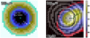 |
Fig. B.2 Left: examples of annular masks created inside and outside of the FWHM ellipse of each core at each wavelength. The example mask image shown here is at 500 μm and belongs to the prestellar core of Fig. B.1. Inside out, the division of the masks along the core radius is the following, considering the FWHM ellipse as 100%: region 1: <60% interior of the FWHM radius, region 2: 60–80%, 3: 80–100%, 4: 100–120%, 5: 120–140%, 6: 140–160%, 7: 160–180%, 8: 180–200%. Region A: <80% (regions 1+2), B: <100% (1+2+3). Right: the first maximum (i.e., the highest intensity pixel) in each mask is shown by a green-shaded diamond in the example image. The panel size, marked source center, and FWHM sizes are the same for each pair of mask image and observed image. |
The automatic post-selection script, written in IDL, works without any free parameter. It performs further source selection and elimination according to the following steps:
- 1.
The script prepares a close-up view of each core from the input source list at the standard HGBS wavelengths (70, 160, 250, 350, 500 μm), and in the high-resolution column density plane (see Figs. A.1, and A.2 for examples). Another example of a core at 500 μm is provided in Fig. B.1. The input source list of the post-selection stage is the output of the core selection procedure detailed in Sect. 3.5.1.
- 2.
Annular masks are created inside and outside of the FWHM ellipse of a given source at each wavelength, which are expanded (or shrunk) versions of the FWHM elliptical footprint, scaling with radius, not with area. The division and numbering of these masks are illustrated in the left panel of Fig. B.2. We split the immediate neighborhood of each candidate core into the following masks, labeled by their linear sizes measured in units of the FWHM size (taken to be100%). Region (1): elliptical area corresponding to a shrunk version of the FWHM footprint, within its 60% linear size; (2): region between the 60% and the 80% ellipse; (3): 80–100% mask; (4): 100–120% mask, (5): 120–140% mask; (6): 140–160% mask; (7): 160–180% mask; (8): 180–200% mask. Region A: elliptical area enclosed within the 80% ellipse (1 + 2); region B: area enclosed within the FWHM elliptical contour (i.e., <100% mask = 1 + 2 + 3).
- 3.
In the next step, maxima are found in the observed images (at 160–250–350–500 μm, and at
 ) under the corresponding rings of masks (see right panel of Fig. B.2). The panel size, marked source center and FWHM sizes are the same for a pair of observed image and mask image at each wavelength. The location of the maximum value (i.e., the highest intensity pixel) in each consecutive annular mask map sections under the masks are is marked by a green-shaded symbol whose size increases with radius from nominal source center. At the same time, the script also locates the second and third intensity maximum points within each annular mask (not shown in Fig. B.2).
 - 4.
At this stage, when a core is post-selected at a certain observed wavelength, its counter flag (cntCoreλ) at that wavelengthis assigned a value of 1, that is, cntCoreλ = 1. The default 0 value of cntCoreλ flips to 1 if:
- I.
the first maximum intensity values under the consecutive masks are decreasing outward from core center,
OR
- II.
the maximum intensity inside the FWHM area (region B) is higher than in the next mask outward (region 4),
OR
- III.
at least two of the secondary maxima in regions 1, 2, and 3 are larger than the first maximum in region 4,
OR
- IV.
the value of the third maximum in region 1 is larger than the first maxima in regions 2 and 3.
AND
- V.
the aspect ratio of the core ellipse is ≤3.
More precisely, at a certain wavelength, a candidate core is post-selected (kept) if at least one of the criteria from [I.] to [IV.] is satisfied, and if criterion [V.] is fulfilled at the same time.
- I.
- 5.
The script then loops over the list of candidate cores to be post-selected, and analyzes each wavelength in turn. The final post-selection of a core is granted if cntCoreλ = 1 in at least three bands among the 160–250–350–500 μm images plus the high-resolution column density map.
In the case of Orion B, the fraction of discarded sources after applying the above procedure was ~ 30% of the input source list.
Our primary intention was to automate the post-selection checks of cores directly from the information contained in the observed Herschel maps, mimicking what a human eye would do. This script greatly facilitates the post-selection evaluation, but a final visual inspection is still recommended. As it was primarily designed for resolved dense cores, this procedure is not optimal for point-like sources or protostars.
Appendix C Completeness of HGBS prestellar core extractions in Orion B
To assess the completeness of the present HGBS census of prestellar cores in Orion B, we used both simulated data and the simple model described in Appendix B.2 of Könyves et al. (2015).
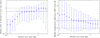 |
Fig. C.1 Left: ratio of measured to true core mass as function of measured core mass for the simulated core extractions. The error bars are ±1σ where σ is the standard deviation of the mass ratio in each mass bin. The median mass ratio is ~ 0.75 for observed core masses between ~0.3 M⊙ and ~ 0.8 M⊙ (as indicated by the horizontal blue line). The horizontal dashed line indicates a mass ratio of 1, as expected for perfect core mass estimates. Right: difference between measured SED temperature and true mass-averaged dust temperature as function of measured core mass for the simulated core extractions. The error bars are ± 1σ where σ is the standard deviation of the temperature difference in each mass bin. The median temperature difference is approximately + 2 K between ~0.3 M⊙ and ~ 0.8 M⊙ (as marked by the horizontal blue line), close to the fiducial completeness limit. The horizontal dashed line indicates no temperaturedifference, as expected for perfect core temperature estimates. |
To simulate core extractions, we constructed clean maps of the background cloud emission at Herschel wavelengths (plus a column density map), by subtracting the compact sources identified with getsources from the observed images (see Sects. 3.4 and 3.5). We then injected model Bonnor-Ebert-like cores within the clean-background maps to produce synthetic Herschel and column density images of the region. We used a population of 711 model starless cores with the following piece-wise power-law mass distribution: ΔN∕ΔlogM ∝ M+1.35 from 0.1 M⊙ to 0.4 M⊙, ΔN∕ΔlogM ∝ M0 from 0.4 M⊙ to 0.9 M⊙, and ΔN∕ΔlogM ∝ M−1.35 from 0.9 M⊙ to 20 M⊙. The positions of the model cores in a mass versus size diagram similar to that shown in Fig. 7 were consistent with critical Bonnor-Ebert isothermal spheres at effective gas temperatures ~ 7–20 K. The far-infrared and submillimeter continuum emission from the synthetic Bonnor–Ebert cores at all Herschel wavelengths was simulated using an extensive grid of spherical dust radiative transfer models generated with the MODUST code (e.g., Bouwman et al. 2000; Bouwman 2001). Accordingly, each synthetic prestellar core had a realistic dust temperature profile with a significantly lower dust temperature in its central inner part, as observed in resolved starless cores (cf. Roy et al. 2014). The synthetic cores were randomly distributed within the portions of the observed field where  cm−2 (or AV≳5), without any mass segregation. Compact source extraction and core selection and classification were subsequently performed with getsources in the same manner as for the real observations (see Sects. 3.4 and 3.5).
As stated in Sect. 3.8 and illustrated in Fig. 8, the results of these Monte–Carlo tests indicate that the present Herschel census of prestellar cores in Orion B is ~ 80% complete down to ~0.5 M⊙ in true core mass.
The above Monte–Carlo simulations were used to estimate the accuracy of the derived parameters such as core mass, radius, and dust temperature by comparing the measured values after core extraction to the intrinsic values of the model cores. Figure C.1 (left) shows that the measured core masses typically underestimate the true core masses by ~ 25% on average, and Fig. C.1 (right) suggests that the derived SED temperatures typically overestimate the true mass-averaged dust temperatures of the cores by typically ~ 2 K, around the fiducial completeness limit of ~0.4 M⊙ in observed mass. A similar comparison for the core sizes (Fig. C.2) indicates that the measured sizes (prior to deconvolution) are within ~5% of the true core sizes on average. Since the core masses are underestimated when the dust temperatures are overestimated, the slight bias of the derived masses (Fig. C.1 left) can be interpreted as a direct consequence of the temperature overestimation (Fig. C.1 right). The latter is because the dust temperature derived from SED fitting exceeds the mass-averaged dust temperature of starless cores owing to the presence of an internal dust temperature gradient rising outward (see, e.g., Roy et al. 2014). Accounting for the ~ 25% effect on the derived masses, we estimate that the ~80% completeness limit at ~0.5 M⊙ in true core mass is located at ~0.4 M⊙ in observed core mass.
Figure C.3 confirms that the prestellar CMF can be reliably determined down to a fiducial completeness limit of ~ 0.4 M⊙ in observed mass. A Kolmogorov–Smirnov (K–S) test shows that the derived CMF (blue histograms in Fig. C.3) is statistically indistinguishable (at the ~90% confidence level) from the input mass function (red curve in Fig. C.3) above 0.4 M⊙. We also point out that the mass function of extracted candidate prestellar cores (light blue histogram in Fig. C.3) starts to deviate from the mass function of robust prestellar cores (dark blue histogram) below ~ 0.4 M⊙, implying that the selection of bona fide self-gravitating starless cores becomes quite uncertain below the fiducial completeness limit. Indeed, the sample of candidate prestellar cores includes a significant number of non-self-gravitating or spurious objects below this limit. Conversely, the sample of robust prestellar cores becomes severely incomplete.
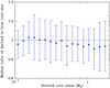 |
Fig. C.2 Ratio of measured to (convolved) intrinsic core size as function of measured core mass for simulated core extractions. The error bars are ±1σ where σ is the standard deviation of the size ratio in each mass bin. The horizontal dashed line indicates a size ratio of 1, as expected forperfect core size estimates. |
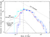 |
Fig. C.3 Synthetic prestellar core mass function (CMF) derived from simulated source extractions (blue histograms) compared to the input mass function of 711 model cores (red curve) constructed as described in the text. The light blue and dark blue histograms show the mass functions of the extracted candidate and robust prestellar cores, respectively. The estimated 80% completeness level of our Herschel census of prestellar cores in Orion B is indicated by the vertical dashed line at 0.4 M⊙ (in observedcore mass). |
As the rms level of background emission fluctuations (often referred to as “cirrus confusion noise”) generally increases with column density (cf. Kiss et al. 2001 and Fig. B.4 in Könyves et al. 2015), the completeness level of our census of prestellar cores is background dependent and becomes worse in areas with higher background cloud emission. To estimate the variations of the completeness level in the observed field, we used the simple model of the core extraction process and completeness problem presented inAppendix B.2 of Könyves et al. (2015) for the Aquila cloud. This model, scaled to the distance of Orion B, allowed us to estimate individual completeness curves as a function of background column density, as shown in Fig. C.4. A global completeness curve (shown by the dashed blue curve in Fig. 8) was then computed as a weighted average of the individual completeness curves using the observed distribution of mass in the cloud as a function of background column density (cf. Fig. 4 here and Appendix B.2 of Könyves et al. 2015 for further details).
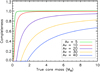 |
Fig. C.4 Model completeness curves of Herschel prestellar core extractions in Orion B for five values of background cloud column density expressed in units of visual extinction from
|


Appendix D Spatial clustering of prestellar cores in different mass regimes
D.1 Clustering of dense cores
The spatial clustering of dense cores can be defined and investigated with many methods (e.g., Kirk et al. 2016b; Gutermuth et al. 2009). Here, we used dendrograms (Rosolowsky et al. 2008) to define groups or clusters of cores. We utilized the IDL functions CLUSTER_TREE and DENDRO_PLOT separately for the robust prespellar core sample in the northern, middle, and southern tiles, separated by the declination lines at Dec2000 = 1° 31′ 55″, and Dec2000 = −0° 28′ 38″. Based on the column density distribution in the entire field, this seems to be a valid choice. A clear and simple example of a hierarchical clustering is shown in Fig. D.1 for the northern region L1622.
In this figure, the labeled individual cores are arranged in the bottom of the dendrogram. In the jargon they are referred to as leaves, marked by the lowest vertical lines, and they have no substructures. The horizontal lines connect leaves, then higher hierarchy levels, making branches. The point where a vertical line originates from a horizontal one is called a “node”. Its height represents the distance (in parsec) between the left and right branches. The elements (i.e., cores) of these branches can also be called clusters.
In order to select clusters for our analysis, the dendrogram trees were inspected, and cores within 3 pc separation of each other in a branch were selected. We required a minimum number of 12 core elements. If a bigger cluster had significant sub-branches, we split it again into smaller clusters, typically at ~ 1.5 − 2 pc distances. Their properties can be studied separately, or together in larger clusters. This way, we found one cluster containing 16 robust prestellar cores around L1622 in the north of Orion B (see Fig. D.1). The left and middle panels of Fig. D.2 (and Fig. D.3) display the various clusters of robust prestellar cores in the NGC 2068 and 2071 regions based on the above selection from their dendrogram trees. The number of core elements in these clusters are as follows: cluster N1: 43 cores, cluster N2: 100, N22: 36, N211: 44, N212: 20.
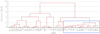 |
Fig. D.1 Dendrogram tree used for selecting cores in L1622. The leaves represent the list of cores in the northern part of Orion B (Dec2000 > 1° 31′ 55″). The 16 cluster members in this case were selected from leaves 6 to 37, marked by the blue rectangle. The red vertical connections projected on the Y axis show the distance between leaves and branches (see text for details). |
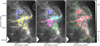 |
Fig. D.2 Clusterings of robust prestellar cores in NGC 2068 and 2071 of Orion B, defined mainly using dendrograms. The selected clusters are displayed in different colors, overplotted on the column density map of NGC 2068 and 2071. The left panel shows a bigger cluster (N2 in yellow), where cores were selected within 3 pc distances from one another in a branch of the dendrogram tree around NGC 2068 and 2071 (see text).A similar dendrogram tree is shown in Fig. D.1 for L1622. The middle panel displays subclusters of the N2 group. The cores within these smaller clusters are closer to each other than ~ 1.5 − 2 pc. In the right image, an arbitrary column density level of about 2 × 1021 cm−2 defines a group of cores in the region of NGC 2068 and 2071. |
The CLUSTER_TREE function was run with the LINKAGE keyword (= 2) which uses a weighted pairwise average. The distance between two leaves and clusters is defined as the average distance for all pairs of objects between each cluster, weighted by the number of objects in each cluster. We chose this method because it works well both for homogeneous clusters and for chain-like clusters. We indeed trace rather elongated, and more compact (sub)clusters as well.
Although these clustering properties stem only from the extracted core positions, the resulted clusters correlate very well with underlying column density features, including filaments, along which most of the cores are found. If we compare Fig. 9 (left panel) and Fig. D.2, we find eye-catching chains of cores along filaments. Using this idea, we also set an arbitrary column density level of about 2 × 1021 cm−2 to select another group of cores in the region of NGC 2068 and 2071 (right panel of Fig. D.2). With various clusters over the same region we can test if certain trends of core properties hold on different spatial scales.
D.2 Mass segregation of dense cores with the MST method
Figure 12 in Sect. 4.2 indicates that the most massive prestellar cores in our sample are spatiallysegregated in the highest column density portions of the Orion B complex. This mass segregation can also be quantified using the minimum spanning tree (MST) technique (e.g., Allison et al. 2009; Parker & Goodwin 2015). We applied this technique to the clusters of dense cores defined with the help of dendrograms in Appendix D.1. The MST method compares the minimum spanning tree of a given number N of the most massive cores with that of a randomly distributed population of cores. The observed and random MSTs are constructed from graphs where the shortest possible separations are calculated between cores, without allowing closed loops. If mass segregation is present, the MST length of the most massive cores in the sample should be significantly shorter than that of a random population of cores. The degree of mass segregation can be quantified via the mass segregation ratio, ΛMSR, defined as the ratio of the average MST length for N randomly chosen cores to the MST length for the N most massive cores in the sample (Allison et al. 2009; Parker 2018). The ΛMSR should significantly exceed 1 when mass segregation is present.
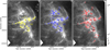 |
Fig. D.3 Alternative groupings of robust prestellar cores in NGC 2068 and 2071. The left panel shows the N2 cluster, the middle panelthe N0 = N1 + N2 clusters (see left panel of Fig. D.2), and the right panel all cores lying above ~2 × 1021 cm−2 in this area (see right panel of Fig. D.2). Black open diamonds mark the 3 (left and middle panels) or 10 (right panel) most massive prestellar cores in these clusters. |
Figure D.4 shows a mass segregation ratio plot, in which MST calculations were applied to the N2 cluster of NGC 2068 and 2071 (see left panel of Fig. D.2). With a sliding window of three cores, the N2 cluster shows an explicit positive mass segregation (ΛMSR > 6), where the most massive cores in this region with M > 10 M⊙ are more concentrated spatially than cores with lower masses (left panel of Fig. D.3). However, comparing and contrasting the panels of Fig. D.3 with the summary table of mass segregation properties in various core clusters (Table D.1), it does not appear obvious that the three most massive cores in the N2 cluster are much more concentrated than the –same– three most massive cores in the N0 (=N1+N2) cluster (see middle panel of Fig. D.3). After carefully inspecting the values in Table D.1, the overall result in NGC 2068 and 2071 provides only marginal evidence for other than a random distribution of core masses, even though in one case the segregation of the most massive cores is strong (i.e., Fig. D.4). Further caveats and assumptions of the ΛMSR method are discussed in detail in, for example, Parker (2018).
Finding some degree of mass segregation at the prestellar core stage in Orion B would lend support to the idea of primordial mass segregation in stellar protoclusters. Mass segregation at birth may be expected since protostellar sources embedded in denser filaments can accrete longer before feedback effects stop further gas inflow. This effect differs from the dynamical mass segregation quickly affecting evolved stars in revealed star clusters (e.g., Kroupa 2008).
Using published dense core samples from both the HGBS and ALMA (Atacama Large Millimeter Array) observations, Dib & Henning (2019) performed structure and mass segregation studies that they linked to the star formation activity of their set of clouds. They claim that the level of core mass segregation is positively correlated with the surface density of the star formation rate in the cloud. They attribute this correlation to a dependence on the physical conditions that have been imprinted by the large scale environment at the time these clouds started to form.
Based on dense cores in Orion B from JCMT’s SCUBA-2 observations, Kirk et al. (2016b) and Parker (2018) analyzed the clustering and mass segregation properties by various methods. While Kirk et al. (2016b) found segregation of massive cores in NGC 2068 and 2071, and in NGC 2023 and 2024, according to Parker (2018), only a mild mass segregation is present in the NGC 2068 and 2071 regions. Our above findings seem to approach these latter results. However, we issue here a word of caution: the conclusions on mass segregation may depend somewhat on the chosen cluster and the exact method of analysis.
D.3 Core masses versus core surface density
As we have shown in Sect. 4.2, the presence of prestellar cores is strongly correlated with the local column density in the ambient cloud. This relationship is perhaps not surprising as dense cores require sufficient gas (at highcolumn- and volume density) to form in the first place. In this appendix we present some initial results on the distributions of cores relative to each other (which will be investigated in more detail in a later paper).
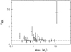 |
Fig. D.4 Mass segregation ratio, ΛMSR, as function of core mass in the N2 cluster of NGC 2068 and 2071, including 100 robust prestellarcores (see left panel of Fig. D.2). The tool used to derive ΛMSR is described in Allison et al. (2009). A sliding window of three cores (N = 3) was set in this case. |
Mass segregation results with ΛMSR method (based on Allison et al. 2009) in various core clusters of NGC 2068 and 2071.
We consider the sample of 423 robust prestellar cores, with masses > 0.4M⊙ above the completeness limit (see Sect. 3.8). The core surface number density, Σcores, is defined from the radius containing the 6 nearest neighbors, r6, as  (cf. Casertano & Hut 1985). Very low values ofΣcores indicate that cores are relatively isolated, very high values of Σcores that there are many cores close-by.
From the results of Sect. 4.2, we know that the most massive cores are in the areas with the highest background column density. An interesting related question to ask is whether the highest-mass cores are also found in regions of highest core surface density. In Fig. D.5, we show a plot of core surface number density (using arbitrary angular area units) against core mass. It is immediately obvious that there is no strong correlation between core mass and core surface density.
We can analyze Fig. D.5 more quantitatively using a Gini-like statistic (Gini 1912; Ward-Duong et al. 2015, see the latter for an astrophysical application). In an ordered list of cores by surface density we can quantify if a subset of cores (e.g., those with the highest masses) are consistent with being randomly distributed in the list (i.e., looking for a bias in what surface density those cores are found at).
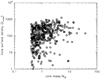 |
Fig. D.5 Distribution of core surface number densities (in angular area units) against core mass (in M⊙). The sample of robust prestellar cores was used above 0.4 M⊙. |
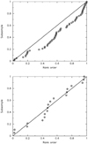 |
Fig. D.6 Cumulative distribution function of core positions (open circles) in ordered list of 423 core surface densities. Top: positions of 62 cores with masses >3 M⊙. Bottom: 19 most massive cores (>7 M⊙). See text for explanation. |
As an example, the upper panel of Fig. D.6 shows the positions in an ordered list of all 423 core surface densities (the x-axis), and a cumulative distribution function (CDF) of the positions of the 62 cores with masses > 3M⊙ (open circles). If the cores with masses >3M⊙ were randomly distributed in the list then we would expect them to roughly follow the diagonal line (i.e., be equally likely to be anywhere inthe list).
Appendix E Additional figures
The clear deviation from randomness can be quantified by calculating the area under the actual distribution and comparing it to a large ensemble of samples of 62 cores taken randomly from the list. If the distribution were random we would expect the area under the CDF to be 0.51 ± 0.03 (1σ error), while the actual area is 0.38. More usefully dividing the true by the expected values we have a quantity  (formally 5σ from random, although the distribution of random areas is not normally distributed in the tails). More qualitatively, this discrepancy is because cores >3M⊙ are very unlikely to be at low core surface densities (only 25% of them are in the lowest 50% of core surface densities), and very likely to be at high core surface density (a third of them are in the top 20% of core surface densities). A strong correlation between core mass and local core surface density was also found based on the SCUBA-2 data in Orion B (Kirk et al. 2016b).
However, if we take only the 19 most massive Herschel cores >7 M⊙, as shown in the lower panel of Fig. D.6, we find that the most massive cores are completely consistent with being randomly distributed in core surface density with  (where unity is consistent with random). This is telling us that all cores with > 3M⊙ have a strong bias to be in regions of high core surface density, the trend is not following a simple higher-mass higher-core surface density relationship, and the very highest-mass cores could be “different” in some way and certainly show no signatures that could be easily interpreted as “mass segregation”.
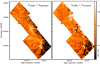 |
Fig. E.1 Left: map of the ratio of AV-converted column density from HGBS data to visual extinction from Bontemps et al. Right: map of the ratio of AV -converted column density from HGBS data to visual extinction from Lombardi et al. The median values of both ratio maps are ~0.5 (see Sect. 3.1 for details). |
 |
Fig. E.2 L1622 cloud and its surroundings. The gray background image shows the mask of filamentary network traced by getfilaments (Men’shchikov 2013). Within the getfilaments mask the color scale represents column density values in the column density map (Fig. 2 left). Angular scales up to 100′′ are shown, which corresponds to ~0.2 pc at d = 400 pc. Left: overplotted thicker blue skeletons mark the robust filament crests from the DisPerSE (Sousbie 2011) sample (see Sect. 3.2 for details). The latter sample together with the thin cyan crests make the DisPerSE raw sample of filaments.Right: overplotted blue crosses mark robust prestellar cores in the northern region. |
 |
Fig. E.3 Ratios of SCUBA-2 to HGBS core mass estimates for matched starless and protostellar pairs within 6′′. The SCUBA-2 core masses were re-derived assuming either 1) the dust temperatures estimated from Herschel SED fitting ( |

References
- Allison, R. J., Goodwin, S. P., Parker, R. J., et al. 2009, MNRAS, 395, 1449 [Google Scholar]
- Alves, J., Lombardi, M., & Lada, C. J. 2017, A&A, 606, L2 [NASA ADS] [CrossRef] [EDP Sciences] [Google Scholar]
- André, P., Belloche, A., Motte, F., & Peretto, N. 2007, A&A, 472, 519 [NASA ADS] [CrossRef] [EDP Sciences] [Google Scholar]
- André, P., Men’shchikov, A., Bontemps, S., et al. 2010, A&A, 518, L102 [NASA ADS] [CrossRef] [EDP Sciences] [Google Scholar]
- André, P., Di Francesco, J., Ward-Thompson, D., et al. 2014, in Protostars and Planets VI, eds. H. Beuther et al. (Tucson: University of Arizona Press), 27 [Google Scholar]
- André, P., Könyves, V., Arzoumanian, D., & Roy, A. 2017, Mem. Soc. Astron. It., 88, 521 [NASA ADS] [Google Scholar]
- André, P., Arzoumanian, D., Könyves, V., Shimajiri, Y., & Palmeirim, P. 2019, A&A, 629, L4 [Google Scholar]
- Arzoumanian, D., André, P., Didelon, P., et al. 2011, A&A, 529, L6 [Google Scholar]
- Arzoumanian, D., André, P., Peretto, N., & Könyves, V. 2013, A&A, 553, A119 [NASA ADS] [CrossRef] [EDP Sciences] [Google Scholar]
- Arzoumanian, D., André, P., Könyves, V., et al. 2019, A&A, 621, A42 [NASA ADS] [CrossRef] [EDP Sciences] [Google Scholar]
- Bally, J. 2008, Handbook of Star Forming Regions, ed. B. Reipurth (San Francisco: ASP), 459 [Google Scholar]
- Beichman, C. A., Myers, P. C., Emerson, J. P., et al. 1986, ApJ, 307, 337 [NASA ADS] [CrossRef] [Google Scholar]
- Benedettini, M., Schisano, E., Pezzuto, S., et al. 2015, MNRAS, 453, 2036 [NASA ADS] [CrossRef] [Google Scholar]
- Benedettini, M., Pezzuto, S., Schisano, E., et al. 2018, A&A, 619, A52 [NASA ADS] [CrossRef] [EDP Sciences] [Google Scholar]
- Bernard, J.-P., Paradis, D., Marshall, D. J., et al. 2010, A&A, 518, L88 [NASA ADS] [CrossRef] [EDP Sciences] [Google Scholar]
- Bohlin, R. C., Savage, B. D., & Drake, J. F. 1978, ApJ, 224, 132 [NASA ADS] [CrossRef] [Google Scholar]
- Bontemps, S., André, P., Könyves, V., et al. 2010, A&A, 518, L85 [NASA ADS] [CrossRef] [EDP Sciences] [Google Scholar]
- Bouwman, J. 2001, PhD Thesis, University of Amsterdam, The Netherlands [Google Scholar]
- Bouwman, J., de Koter, A., van den Ancker, M. E., & Waters, L. B. F. M. 2000, A&A, 360, 213 [NASA ADS] [Google Scholar]
- Bresnahan, D., Ward-Thompson, D., Kirk, J. M., et al. 2018, A&A, 615, A125 [NASA ADS] [CrossRef] [EDP Sciences] [Google Scholar]
- Bron, E., Daudon, C., Pety, J., et al. 2018, A&A, 610, A12 [NASA ADS] [CrossRef] [EDP Sciences] [Google Scholar]
- Casertano, S., & Hut, P. 1985, ApJ, 298, 80 [Google Scholar]
- Chabrier, G. 2005, Astrophys. Space Sci. Lib., 327, 41 [NASA ADS] [CrossRef] [Google Scholar]
- Cox, N. L. J., Arzoumanian, D., André, P., et al. 2016, A&A, 590, A110 [NASA ADS] [CrossRef] [EDP Sciences] [Google Scholar]
- Dib, S., & Henning, T. 2019, A&A, 629, A135 [NASA ADS] [CrossRef] [EDP Sciences] [Google Scholar]
- Dunham, M. M., Crapsi, A., Evans, II, N. J., et al. 2008, ApJS, 179, 249 [NASA ADS] [CrossRef] [Google Scholar]
- Elmegreen, B. G., & Falgarone, E. 1996, ApJ, 471, 816 [NASA ADS] [CrossRef] [Google Scholar]
- Evans, II, N. J., Dunham, M. M., Jørgensen, J. K., et al. 2009, ApJS, 181, 321 [NASA ADS] [CrossRef] [Google Scholar]
- Finkbeiner, D. P. 2003, ApJS, 146, 407 [NASA ADS] [CrossRef] [Google Scholar]
- Gini, C. 1912, in Variabilità e mutabilità, Reprinted in Memorie di Metodologia Statistica (eds. E. Pizetti, T. Salvemini), Rome: Libreria Erendi Virgilio Veschi (Berlin: Springer), 1955 [Google Scholar]
- Griffin, M. J., Abergel, A., Abreu, A., et al. 2010, A&A, 518, L3+ [Google Scholar]
- Gutermuth, R. A., Megeath, S. T., Myers, P. C., et al. 2009, ApJS, 184, 18 [NASA ADS] [CrossRef] [Google Scholar]
- Hatchell, J., Richer, J. S., Fuller, G. A., et al. 2005, A&A, 440, 151 [NASA ADS] [CrossRef] [EDP Sciences] [Google Scholar]
- Hennemann, M., Motte, F., Schneider, N., et al. 2012, A&A, 543, L3 [NASA ADS] [CrossRef] [EDP Sciences] [Google Scholar]
- Heyer, M., Krawczyk, C., Duval, J., & Jackson, J. M. 2009, ApJ, 699, 1092 [NASA ADS] [CrossRef] [Google Scholar]
- Hildebrand, R. H. 1983, QJRAS, 24, 267 [NASA ADS] [Google Scholar]
- Inutsuka, S.-I., & Miyama, S. M. 1997, ApJ, 480, 681 [NASA ADS] [CrossRef] [Google Scholar]
- Johnstone, D., Di Francesco, J., & Kirk, H. 2004, ApJ, 611, L45 [Google Scholar]
- Kirk, H., Di Francesco, J., Johnstone, D., et al. 2016a, ApJ, 817, 167 [NASA ADS] [CrossRef] [Google Scholar]
- Kirk, H., Johnstone, D., Di Francesco, J., et al. 2016b, ApJ, 821, 98 [Google Scholar]
- Kiss, C., Ábrahám, P., Klaas, U., Juvela, M., & Lemke, D. 2001, A&A, 379, 1161 [NASA ADS] [CrossRef] [EDP Sciences] [Google Scholar]
- Koch, E. W., & Rosolowsky, E. W. 2015, MNRAS, 452, 3435 [NASA ADS] [CrossRef] [Google Scholar]
- Könyves, V., André, P., Men’shchikov, A., et al. 2010, A&A, 518, L106 [NASA ADS] [CrossRef] [EDP Sciences] [Google Scholar]
- Könyves, V., André, P., Men’shchikov, A., et al. 2015, A&A, 584, A91 [NASA ADS] [CrossRef] [EDP Sciences] [Google Scholar]
- Kramer, C., Stutzki, J., Rohrig, R., & Corneliussen, U. 1998, A&A, 329, 249 [NASA ADS] [Google Scholar]
- Kroupa, P. 2001, MNRAS, 322, 231 [NASA ADS] [CrossRef] [Google Scholar]
- Kroupa, P. 2008, IAU Symp., 246, 13 [NASA ADS] [Google Scholar]
- Lada, C. J., Forbrich, J., Lombardi, M., & Alves, J. F. 2012, ApJ, 745, 190 [NASA ADS] [CrossRef] [Google Scholar]
- Ladjelate, B., André, P., Könyves, V., et al. 2019, A&A, accepted [Google Scholar]
- Lallement, R., Vergely, J.-L., Valette, B., et al. 2014, A&A, 561, A91 [NASA ADS] [CrossRef] [EDP Sciences] [Google Scholar]
- Lombardi, M. 2009, A&A, 493, 735 [NASA ADS] [CrossRef] [EDP Sciences] [Google Scholar]
- Markwardt, C. B. 2009, ASP Conf. Ser., 411, 251 [Google Scholar]
- Marsh, K. A., Griffin, M. J., Palmeirim, P., et al. 2014, MNRAS, 439, 3683 [NASA ADS] [CrossRef] [Google Scholar]
- Marsh, K. A., Kirk, J. M., André, P., et al. 2016, MNRAS, 459, 342 [NASA ADS] [CrossRef] [Google Scholar]
- Megeath, S. T., Gutermuth, R., Muzerolle, J., et al. 2012, AJ, 144, 192 [NASA ADS] [CrossRef] [Google Scholar]
- Megeath, S. T., Gutermuth, R., Muzerolle, J., et al. 2016, AJ, 151, 5 [NASA ADS] [CrossRef] [Google Scholar]
- Men’shchikov, A. 2013, A&A, 560, A63 [NASA ADS] [CrossRef] [EDP Sciences] [Google Scholar]
- Men’shchikov, A. 2017, A&A, 607, A64 [NASA ADS] [CrossRef] [EDP Sciences] [Google Scholar]
- Men’shchikov, A., André, P., Didelon, P., et al. 2012, A&A, 542, A81 [NASA ADS] [CrossRef] [EDP Sciences] [Google Scholar]
- Menten, K. M., Reid, M. J., Forbrich, J., & Brunthaler, A. 2007, A&A, 474, 515 [NASA ADS] [CrossRef] [EDP Sciences] [Google Scholar]
- Myers, P. C. 1983, ApJ, 270, 105 [NASA ADS] [CrossRef] [Google Scholar]
- Nielbock, M., Launhardt, R., Steinacker, J., et al. 2012, A&A, 547, A11 [NASA ADS] [CrossRef] [EDP Sciences] [Google Scholar]
- Ochsendorf, B. B., Brown, A. G. A., Bally, J., & Tielens, A. G. G. M. 2015, ApJ, 808, 111 [NASA ADS] [CrossRef] [Google Scholar]
- Oliver, S. J., Wang, L., Smith, A. J., et al. 2010, A&A, 518, L21 [NASA ADS] [CrossRef] [EDP Sciences] [Google Scholar]
- Oliver, S. J., Bock, J., Altieri, B., et al. 2012, MNRAS, 424, 1614 [NASA ADS] [CrossRef] [EDP Sciences] [Google Scholar]
- Onishi, T., Mizuno, A., Kawamura, A., Ogawa, H., & Fukui, Y. 1998, ApJ, 502, 296 [NASA ADS] [CrossRef] [Google Scholar]
- Orkisz, J. H., Pety, J., Gerin, M., et al. 2017, A&A, 599, A99 [NASA ADS] [CrossRef] [EDP Sciences] [Google Scholar]
- Ostriker, J. 1964, ApJ, 140, 1056 [NASA ADS] [CrossRef] [MathSciNet] [Google Scholar]
- Palmeirim, P., André, P., Kirk, J., et al. 2013, A&A, 550, A38 [NASA ADS] [CrossRef] [EDP Sciences] [Google Scholar]
- Parker, R. J. 2018, MNRAS, 476, 617 [Google Scholar]
- Parker, R. J., & Goodwin, S. P. 2015, MNRAS, 449, 3381 [NASA ADS] [CrossRef] [Google Scholar]
- Pety, J., Guzmán, V. V., Orkisz, J. H., et al. 2017, A&A, 599, A98 [NASA ADS] [CrossRef] [EDP Sciences] [Google Scholar]
- Pezzuto, S., Benedettini, M., Di Francesco, J., et al. 2019, A&A, submitted [Google Scholar]
- Pilbratt, G. L., Riedinger, J. R., Passvogel, T., et al. 2010, A&A, 518, L1 [CrossRef] [EDP Sciences] [Google Scholar]
- Poglitsch, A., Waelkens, C., Geis, N., et al. 2010, A&A, 518, L2 [NASA ADS] [CrossRef] [EDP Sciences] [Google Scholar]
- Polychroni, D., Schisano, E., Elia, D., et al. 2013, ApJ, 777, L33 [NASA ADS] [CrossRef] [Google Scholar]
- Pon, A., Ochsendorf, B. B., Alves, J., et al. 2016, ApJ, 827, 42 [NASA ADS] [CrossRef] [Google Scholar]
- Press, W. H., Teukolsky, S. A., Vetterling, W. T., & Flannery, B. P. 1992, Numerical recipes in FORTRAN. The art of scientific computing, 2nd edn., (Cambridge: CambridgeUniversity Press) [Google Scholar]
- Rosolowsky, E. W., Pineda, J. E., Kauffmann, J., & Goodman, A. A. 2008, ApJ, 679, 1338 [NASA ADS] [CrossRef] [Google Scholar]
- Roy, A., André, P., Palmeirim, P., et al. 2014, A&A, 562, A138 [NASA ADS] [CrossRef] [EDP Sciences] [Google Scholar]
- Schneider, N., Bontemps, S., Simon, R., et al. 2011, A&A, 529, A1 [NASA ADS] [CrossRef] [EDP Sciences] [Google Scholar]
- Schneider, N., André, P., Könyves, V., et al. 2013, ApJ, 766, L17 [NASA ADS] [CrossRef] [Google Scholar]
- Shimajiri, Y., André, P., Braine, J., et al. 2017, A&A, 604, A74 [NASA ADS] [CrossRef] [EDP Sciences] [Google Scholar]
- Shimajiri, Y., André, P., Ntormousi, E., et al. 2019, A&A, 632, A83 [NASA ADS] [CrossRef] [EDP Sciences] [Google Scholar]
- Sousbie, T. 2011, MNRAS, 414, 350 [NASA ADS] [CrossRef] [Google Scholar]
- Tafalla, M., Myers, P. C., Caselli, P., Walmsley, C. M., & Comito, C. 2002, ApJ, 569, 815 [NASA ADS] [CrossRef] [Google Scholar]
- Ward-Duong, K., Patience, J., De Rosa, R. J., et al. 2015, MNRAS, 449, 2618 [NASA ADS] [CrossRef] [Google Scholar]
- Ward-Thompson, D., André, P., Crutcher, R., et al. 2007, in Protostars and Planets V, eds. B. Reipurth et al. (Tucson: University of Arizona Press), 33 [Google Scholar]
- Zucker, C., Speagle, J. S., Schlafly, E. F., et al. 2019, ApJ, 879, 125 [NASA ADS] [CrossRef] [Google Scholar]
The HGBS first-generation catalog of cores presented in this paper (see Appendix A) was produced with the “November 2013” major release of getsources (v1.140127), which is publicly available from http://gouldbelt-herschel.cea.fr/getsources.
We adopt the same typical internal core temperature of 10 K in Orion B as in the Aquila cloud (cf. Sect. 4.7 of Könyves et al. 2015) since the dust temperature maps derived from Herschel data suggest that the average radiation field is similar in both cloud complexes, with the possible exception of the vicinity of the bright HII region NGC 2024 (see Table 6 of Shimajiri et al. 2017). We also stress that radiative transfer models suggest that the internal temperature of starless dense cores depends only weakly on the ambient radiation field, in contrast to the temperature of the core outer layers.
All Tables
Catalog of dense cores identified in HGBS maps of Orion B (template, full catalog only provided at the CDS).
Derived properties of dense cores identified in HGBS maps of Orion B (template, full table only provided at the CDS).
Mass segregation results with ΛMSR method (based on Allison et al. 2009) in various core clusters of NGC 2068 and 2071.
All Figures
|
Fig. 1 Large-scale view of the Orion-Eridanus superbubble (which reaches beyond Barnard’s Loop) and star-forming clouds along its wall. The color background shows Planck 857 GHz (350 μm) emission (Public Data Release 2, PR2), and the overplotted gray features represent Hα emission (Finkbeiner 2003). The region analyzed in this paper is outlined in white. (PR2 is described in the Planck 2015 Release Explanatory Supplement which is available at https://wiki.cosmos.esa.int/planckpla2015/). |
| In the text | |
|
Fig. 2 Left: H2 column density map of Orion B at 18.2′′ angular resolution, derived from HGBS data. The contours correspond to AV ~ 3 (cyan) and 7 mag (black) in a column density map smoothed to a resolution of 2′. Right: dust temperature map of the Orion B region at 36.3′′ resolution, as derived from the same data set. Blue stars mark the NGC 2023 and 2024, NGC 2068 and 2071 HII regions and reflection nebulae, and the L1622 cometary cloud. The position of the Horsehead Nebula is also shown. |
| In the text | |
|
Fig. 3 Filament networks identified in the subregions NGC 2068 and 2071 (left), and NGC 2023 and 2024 (right). The gray background image displays the mask of the filamentary network traced with getfilaments (Men’shchikov 2013). The overplotted thick blue skeletons mark the robust filament crests identified with the DisPerSE algorithm (Sousbie 2011, see Sect. 3.2 for details). Together with the additional thin cyan crests, these filament crests make up the entire raw sample of DisPerSE filaments. Within the getfilaments mask, the gray scale is the same in both panels, and reflects column density values in the column density map (Fig. 2 left). Transverse angular scales up to 100′′ are shown, corresponding to ~0.2 pc at d = 400 pc. Figure E.2 (left) shows a similar view for the L1622 cloud. |
| In the text | |
|
Fig. 4 Left: high-resolution |
| In the text | |
|
Fig. 5 High-resolution (~18″) column density map of Orion B, derived from SPIRE and PACS observations. The positions of the 1768 identified starless cores (green triangles), 490 robust prestellar cores (blue triangles), and 76 embedded protostellar cores (red symbols) are overplotted. The vast majority of the cores lie in high column density areas. The white declination line at Dec2000 = 1° 31′ 55″ marks the lower boundary of the northern region where cores may be associated with the Barnard’s Loop and at a more uncertain distance (d ~ 170–400 pc). See Sects. 1 and 3.5.2 for details. |
| In the text | |
|
Fig. 6 Distributions of beam-averaged column densities (left) and beam-averaged volume densities (right) at resolution of SPIRE 500 μm observations for 1768 starless cores (green), 804 candidate prestellar cores (light blue), and 490 robust prestellar cores (dark blue curve) in Orion B. |
| In the text | |
|
Fig. 7 Mass versus size diagram for all 1768 starless cores (triangles) identified with Herschel in Orion B, including the 804 candidate prestellar cores (light or dark blue triangles) and 490 robust prestellar cores (filled triangles in dark blue). The core FWHM sizes were measured with getsources in the high-resolution column density map (Fig. 2 left) and deconvolved from an 18.2′′ (HPBW) Gaussian beam. The corresponding physical |
| In the text | |
|
Fig. 8 Completeness curve of candidate prestellar cores as function of true core mass (solid line), which was estimated from Monte–Carlo simulations (see Sect. 3.8). For comparison, the global completeness curve of the model introduced at the end of Appendix C is shown by the dashed blue line. |
| In the text | |
|
Fig. 9 Spatial distributions of robust prestellar cores (blue symbols) overplotted on the filament networks (gray background images) traced with getfilaments in NGC 2068 and 2071 (left), and NGC 2023 and 2024 (right). Transverse angular scales up to 100′′ across the filament footprints are shown here, corresponding to ~0.2 pc at d = 400 pc. In both panels, the color scale displayed within the filament mask corresponds to column density values in the original column density map (Fig. 2 left). See Fig. E.2 (right) for a similar view in the case of L1622. |
| In the text | |
|
Fig. 10 Distribution of separations between dense cores and the nearest filament crests in the DisPerSE raw sample of filaments. The green histogram is for all 1768 starless cores, the light blue histogram for the 804 candidate prestellar cores, and the dark blue histogram for the 490 robust prestellar cores. The vertical lines mark the half widths (i.e., on either side of the filament crests) of a 0.1 pc-wide (red), 0.5 × 0.1 pc-wide (inner black), and a 2 × 0.1 pc-wide (outer black) filament. |
| In the text | |
|
Fig. 11 Distribution of nearest-neighbor core separations in Orion B. The green, light-, and dark blue histograms show the distributions of nearest-neighbor separations for starless cores (either bound or unbound), candidate prestellar cores, and robust prestellar cores, respectively. In each case, only the separations between cores of the same category were considered. The median core separation is ~ 0.14 pc for all three core samples. |
| In the text | |
|
Fig. 12 Top: median prestellar core mass versus background column density (black triangles). The error bars correspond to the inter-quartile range in observed masses for each bin of background column density. The solid, dashed and dotted blue lines are linear fits to the observed median, upper-quartile, and lower-quartile masses as function of background column density, respectively. The red curve shows how the mass at the 50% completeness level varies with background column density according to the model completeness curves of Appendix C (see Fig. C.4). The upper x-axis provides an approximate mass-per-unit-length scale, assuming the local backgroundaround each core is dominated by the contribution of a parent filament with a characteristic width Wfil = 0.1 pc (see end of Sect. 4.5). Bottom: same as upper panel after correcting the distribution of observed core masses for incompleteness effects before estimating the median core mass and inter-quartile range in each column density bin (see Sect. 4.2). Both the median prestellar core mass and the dispersion in core masses increase roughly linearly with background column density. |
| In the text | |
|
Fig. 13 Differential core mass function (ΔN/ΔlogM) of the 1768starless cores (green histogram), 804 candidate prestellar cores (light blue histogram), and 490 robust
prestellar cores (dark blue histogram) identified with Herschel in the whole Orion B field. The error bars correspond to
|
| In the text | |
|
Fig. 14 Comparison of the differential CMF (ΔN/ΔlogM) derived for the 558 candidate prestellar cores lying in areas of low background column density ( |
| In the text | |
|
Fig. 15 Comparison of the global column density PDF in Orion B (blue histogram) to the column density PDF measured after subtraction of dense cores (red solid line) and the PDF measured after subtraction of both dense cores and filaments (black solid line with statistical error bars). The blue histogram is identical to that shown in Fig. 4 (left). The vertical dashed line marks the approximate separation between low-to-intermediate and high column density values at
|
| In the text | |
|
Fig. 16 Differential core formation efficiency (CFE) as function of ambient cloud column density expressed in AV units (blue histogram with error bars), obtained by dividing the mass in the form of candidate prestellar cores in a given column density bin by the cloud mass observed in the same column density bin. The upper x-axis provides an approximate mass-per-unit-length scale, assuming the local background around each core is dominated by the contribution of a parent filament with a characteristic width
Wfil = 0.1 pc (see end of Sect. 4.5). The vertical dashed line marks the fiducial threshold at
|
| In the text | |
|
Fig. 17 Top: total mass in form of prestellar cores as function of ambient cloud column density in Orion B (blue histogram). Bottom: distribution of background column densities for the 490 robust prestellar cores (blue histogram). The vertical dashed lines mark
|
| In the text | |
|
Fig. A.1 Example blow-up Herschel images at 70–160–250–350–500 μm and high-resolution column density map for a (bound) prestellar core. Ellipses represent the estimated major andminor FWHM sizes of the core at each wavelength; they are shown as solid or dashed curves depending on whether the core is significantly detected or not, respectively, at a particular wavelength. See Table A.2 for the physical radius of the core and other derived properties. An angular scale of 30′′ (~ 0.058 pc at d = 400 pc) is shown at the bottom right. North is up, east is left. Similar image cutouts are provided online for all selected starless cores. |
| In the text | |
|
Fig. A.2 Same as Fig. A.1 for a protostellar core. See Table A.2 for its derived properties. Similar image cutouts are provided online for all selected protostellar cores. |
| In the text | |
|
Fig. B.1 Close-up view of a post-selected prestellar core at 500 μm (shown in Fig. A.1) illustrating the post-selection procedure. At each wavelength, the map colorscale is optimizedfor the immediate neighborhood of the core; the lowest and highest map values in the considered box are blanked by black and white colors, respectively. The source center position is marked by a cross, and the FWHM ellipse automatically derived by getsources is plotted. |
| In the text | |
|
Fig. B.2 Left: examples of annular masks created inside and outside of the FWHM ellipse of each core at each wavelength. The example mask image shown here is at 500 μm and belongs to the prestellar core of Fig. B.1. Inside out, the division of the masks along the core radius is the following, considering the FWHM ellipse as 100%: region 1: <60% interior of the FWHM radius, region 2: 60–80%, 3: 80–100%, 4: 100–120%, 5: 120–140%, 6: 140–160%, 7: 160–180%, 8: 180–200%. Region A: <80% (regions 1+2), B: <100% (1+2+3). Right: the first maximum (i.e., the highest intensity pixel) in each mask is shown by a green-shaded diamond in the example image. The panel size, marked source center, and FWHM sizes are the same for each pair of mask image and observed image. |
| In the text | |
|
Fig. C.1 Left: ratio of measured to true core mass as function of measured core mass for the simulated core extractions. The error bars are ±1σ where σ is the standard deviation of the mass ratio in each mass bin. The median mass ratio is ~ 0.75 for observed core masses between ~0.3 M⊙ and ~ 0.8 M⊙ (as indicated by the horizontal blue line). The horizontal dashed line indicates a mass ratio of 1, as expected for perfect core mass estimates. Right: difference between measured SED temperature and true mass-averaged dust temperature as function of measured core mass for the simulated core extractions. The error bars are ± 1σ where σ is the standard deviation of the temperature difference in each mass bin. The median temperature difference is approximately + 2 K between ~0.3 M⊙ and ~ 0.8 M⊙ (as marked by the horizontal blue line), close to the fiducial completeness limit. The horizontal dashed line indicates no temperaturedifference, as expected for perfect core temperature estimates. |
| In the text | |
|
Fig. C.2 Ratio of measured to (convolved) intrinsic core size as function of measured core mass for simulated core extractions. The error bars are ±1σ where σ is the standard deviation of the size ratio in each mass bin. The horizontal dashed line indicates a size ratio of 1, as expected forperfect core size estimates. |
| In the text | |
|
Fig. C.3 Synthetic prestellar core mass function (CMF) derived from simulated source extractions (blue histograms) compared to the input mass function of 711 model cores (red curve) constructed as described in the text. The light blue and dark blue histograms show the mass functions of the extracted candidate and robust prestellar cores, respectively. The estimated 80% completeness level of our Herschel census of prestellar cores in Orion B is indicated by the vertical dashed line at 0.4 M⊙ (in observedcore mass). |
| In the text | |
|
Fig. C.4 Model completeness curves of Herschel prestellar core extractions in Orion B for five values of background cloud column density expressed in units of visual extinction from
|
| In the text | |
|
Fig. D.1 Dendrogram tree used for selecting cores in L1622. The leaves represent the list of cores in the northern part of Orion B (Dec2000 > 1° 31′ 55″). The 16 cluster members in this case were selected from leaves 6 to 37, marked by the blue rectangle. The red vertical connections projected on the Y axis show the distance between leaves and branches (see text for details). |
| In the text | |
|
Fig. D.2 Clusterings of robust prestellar cores in NGC 2068 and 2071 of Orion B, defined mainly using dendrograms. The selected clusters are displayed in different colors, overplotted on the column density map of NGC 2068 and 2071. The left panel shows a bigger cluster (N2 in yellow), where cores were selected within 3 pc distances from one another in a branch of the dendrogram tree around NGC 2068 and 2071 (see text).A similar dendrogram tree is shown in Fig. D.1 for L1622. The middle panel displays subclusters of the N2 group. The cores within these smaller clusters are closer to each other than ~ 1.5 − 2 pc. In the right image, an arbitrary column density level of about 2 × 1021 cm−2 defines a group of cores in the region of NGC 2068 and 2071. |
| In the text | |
|
Fig. D.3 Alternative groupings of robust prestellar cores in NGC 2068 and 2071. The left panel shows the N2 cluster, the middle panelthe N0 = N1 + N2 clusters (see left panel of Fig. D.2), and the right panel all cores lying above ~2 × 1021 cm−2 in this area (see right panel of Fig. D.2). Black open diamonds mark the 3 (left and middle panels) or 10 (right panel) most massive prestellar cores in these clusters. |
| In the text | |
|
Fig. D.4 Mass segregation ratio, ΛMSR, as function of core mass in the N2 cluster of NGC 2068 and 2071, including 100 robust prestellarcores (see left panel of Fig. D.2). The tool used to derive ΛMSR is described in Allison et al. (2009). A sliding window of three cores (N = 3) was set in this case. |
| In the text | |
|
Fig. D.5 Distribution of core surface number densities (in angular area units) against core mass (in M⊙). The sample of robust prestellar cores was used above 0.4 M⊙. |
| In the text | |
|
Fig. D.6 Cumulative distribution function of core positions (open circles) in ordered list of 423 core surface densities. Top: positions of 62 cores with masses >3 M⊙. Bottom: 19 most massive cores (>7 M⊙). See text for explanation. |
| In the text | |
|
Fig. E.1 Left: map of the ratio of AV-converted column density from HGBS data to visual extinction from Bontemps et al. Right: map of the ratio of AV -converted column density from HGBS data to visual extinction from Lombardi et al. The median values of both ratio maps are ~0.5 (see Sect. 3.1 for details). |
| In the text | |
|
Fig. E.2 L1622 cloud and its surroundings. The gray background image shows the mask of filamentary network traced by getfilaments (Men’shchikov 2013). Within the getfilaments mask the color scale represents column density values in the column density map (Fig. 2 left). Angular scales up to 100′′ are shown, which corresponds to ~0.2 pc at d = 400 pc. Left: overplotted thicker blue skeletons mark the robust filament crests from the DisPerSE (Sousbie 2011) sample (see Sect. 3.2 for details). The latter sample together with the thin cyan crests make the DisPerSE raw sample of filaments.Right: overplotted blue crosses mark robust prestellar cores in the northern region. |
| In the text | |
|
Fig. E.3 Ratios of SCUBA-2 to HGBS core mass estimates for matched starless and protostellar pairs within 6′′. The SCUBA-2 core masses were re-derived assuming either 1) the dust temperatures estimated from Herschel SED fitting ( |
| In the text | |
Current usage metrics show cumulative count of Article Views (full-text article views including HTML views, PDF and ePub downloads, according to the available data) and Abstracts Views on Vision4Press platform.
Data correspond to usage on the plateform after 2015. The current usage metrics is available 48-96 hours after online publication and is updated daily on week days.
Initial download of the metrics may take a while.