| Issue |
A&A
Volume 689, September 2024
|
|
|---|---|---|
| Article Number | A3 | |
| Number of page(s) | 16 | |
| Section | Interstellar and circumstellar matter | |
| DOI | https://doi.org/10.1051/0004-6361/202449853 | |
| Published online | 27 August 2024 | |
Probing the filamentary nature of star formation in the California giant molecular cloud★
1
National Astronomical Observatories, Chinese Academy of Sciences,
Beijing
100101, PR China
e-mail: This email address is being protected from spambots. You need JavaScript enabled to view it.
2
Université Paris-Saclay, Université Paris Cité, CEA, CNRS, AIM,
91191
Gif-sur-Yvette, France
e-mail: This email address is being protected from spambots. You need JavaScript enabled to view it.
; This email address is being protected from spambots. You need JavaScript enabled to view it.
Received:
5
March
2024
Accepted:
6
June
2024
Abstract
Context. Recent studies suggest that filamentary structures are representative of the initial conditions of star formation in molecular clouds and support a filament paradigm for star formation, potentially accounting for the origin of the stellar initial mass function (IMF). The detailed, local physical properties of molecular filaments remain poorly characterized, however.
Aims. Using Herschel imaging observations of the California giant molecular cloud, we aim to further investigate the filament paradigm for low- to intermediate-mass star formation and to better understand the exact role of filaments in the origin of stellar masses.
Methods. Using the multiscale, multiwavelength extraction method getsf, we identify starless cores, protostars, and filaments in the Herschel data set and separate these components from the background cloud contribution to determine accurate core and filament properties.
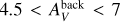
Results. We find that filamentary structures contribute approximately 20% of the overall mass of the California cloud, while compact sources such as dense cores contribute a mere 2% of the total mass. Considering only dense gas (defined as gas with AV,bg > 4.5–7), filaments and cores contribute ~66–73% and 10–14% of the dense gas mass, respectively. The transverse half-power diameter measured for California molecular filaments has a median undeconvolved value of 0.18 pc, consistent within a factor of 2 with the typical ~0.1 pc width of nearby filaments from the Herschel Gould Belt survey. A vast majority of identified prestellar cores (~82–90%) are located within ~0.1 pc of the spines of supercritical filamentary structures. Both the prestellar core mass function (CMF) and the distribution of filament masses per unit length or filament line mass function (FLMF) are consistent with power-law distributions at the high-mass end, ΔN/ΔlogM ∝ M−1.4±0.2 at M > 1 M⊙ for the CMF and ΔN/Δlog Mline ∝ Mline−1.5±0.2 for the FLMF at Mline > 10 M⊙ pc−1, which are both consistent with the Salpeter power-law IMF. Based on these results, we propose a revised model for the origin of the CMF in filaments, whereby the global prestellar CMF in a molecular cloud arises from the integration of the CMFs generated by individual thermally supercritical filaments within the cloud.
Conclusions. Our findings support the existence a tight connection between the FLMF and the CMF/IMF and suggests that filamentary structures represent a critical evolutionary step in establishing a Salpeter-like mass function.
Key words: stars: formation / ISM: clouds / dust, extinction / ISM: structure
The 18.2″ column density map (cf. Fig. 2), and the filament skeleton map (cf. Fig. 7) in FITS format are publicly available at the CDS via anonymous ftp to cdsarc.cds.unistra.fr (130.79.128.5) or via https://cdsarc.cds.unistra.fr/viz-bin/cat/J/A+A/689/A3
© The Authors 2024
 Open Access article, published by EDP Sciences, under the terms of the Creative Commons Attribution License (https://creativecommons.org/licenses/by/4.0), which permits unrestricted use, distribution, and reproduction in any medium, provided the original work is properly cited.
This article is published in open access under the Subscribe to Open model. This email address is being protected from spambots. You need JavaScript enabled to view it. to support open access publication.
1 Introduction
Imaging surveys of Galactic molecular clouds with the Herschel Space Observatory have revolutionized our understanding of the link between the structure of the cold interstellar medium (ISM) and the star formation process, emphasizing the role of filamentary structures (e.g., André et al. 2010; Molinari et al. 2010; Henning et al. 2010; Hill et al. 2011; Juvela et al. 2012). While the existence of filamentary structures in molecular clouds has been known for a long time (e.g., Schneider & Elmegreen 1979; Bally et al. 1987; Myers 2009), Herschel observations have demonstrated that filaments are truly ubiquitous in the cold ISM (e.g., Men’shchikov et al. 2010) and that they make up a dominant fraction of the dense gas in molecular clouds (Schisano et al. 2014; Könyves et al. 2015). The observed filaments display a high degree of universality in their properties (Arzoumanian et al. 2011) and are the prime birthplaces of prestellar cores (e.g., André et al. 2010). In particular, results of the Herschel Gould Belt Survey (HGBS) in nearby molecular clouds (d < 500 pc) indicate that molecular filaments have a typical inner width of ~0.1 pc (Arzoumanian et al. 2011, 2019), and that ~75% of prestellar cores form within dense, thermally supercritical filaments, with masses per unit length (hereafter line masses for short) Mline larger than ~16 M⊙ pc−1, equivalent to gas surface densities above ~160 M⊙ pc−2 (or AV ~8) (Könyves et al. 2015).
These findings support a filament paradigm for low-mass star formation in two main steps (e.g., André et al. 2014): (1) large-scale compression of interstellar material in supersonic magneto-hydrodynamic (MHD) flows generates a cobweb of molecular filaments in the ISM; (2) the densest filaments fragment into prestellar cores by gravitational instability near or above the critical line mass of nearly isothermal, cylindrical filaments (cf. Inutsuka & Miyama 1997), Mline,crit = 2 cs/G (~16 M⊙ pc−1 for molecular gas at ~ 10 K). While the details of this filament scenario remain actively debated, there is little doubt that dense molecular filaments are representative of the initial conditions of at least low-mass star formation (Hacar et al. 2023; Pineda et al. 2023). Since real filaments are not straight, uniform cylinders but exhibit bends and density fluctuations along their lengths, it is important to stress that it is the local rather than the average value of the mass per unit length of a filament that determines its ability to fragment (cf. Inutsuka 2001; Heigl et al. 2018).
The Herschel observations also confirm the existence of a close relationship between the prestellar core mass function (CMF) and the stellar initial mass function (IMF) in the regime of low to intermediate stellar masses (~0.1–5 M⊙ – Könyves et al. 2015; Marsh et al. 2016; Di Francesco et al. 2020), and suggest a connection between the CMF/IMF and the filament line mass function or FLMF (André et al. 2019). Indeed, while the mass function of molecular clouds and clumps within clouds is significantly shallower than the Salpeter IMF ( for clouds/clumps vs.
  for stars above 1 M⊙ – e.g., Salpeter 1955; Solomon et al. 1987; Kramer et al. 1998) the FLMF derived from Herschel data for the sample of HGBS filaments analyzed by Arzoumanian et al. (2019) is much more similar to the Salpeter IMF, with
  above the thermally critical line mass of ~16 M⊙ pc−1 (André et al. 2019). This suggests that molecular filaments may represent the key evolutionary step during the non-linear growth of interstellar structures at which a Salpeter-like mass function is established.
The California giant molecular cloud (California GMC) belongs to the Taurus-Auriga-California-Perseus complex (TACP), as illustrated in Fig. 1. The four giant molecular clouds on the right-hand side surround a region devoid of dust, CO, and HI (Lim et al. 2013). That void is filled, however, with the Hα emission from hydrogen atoms ionized by massive stars (Finkbeiner 2003). The California GMC is located at the front end of a HI supershell (Shimajiri et al. 2019b), and its large-scale morphology, revealed by 13CO emission, is dominated by a continuous filamentary shape over >70 pc (Guo et al. 2021). The supernova explosions in the Per OB2 association may have created this HI supershell and pushed the gas forward (Sancisi et al. 1974; Hartmann & Burton 1997). The California GMC was named “Auriga” in the GouldsBelt Spitzer Legacy Survey (Allen et al. 2006), and therefore also named “Auriga-California” by Harvey et al. (2013) and Broekhoven-Fiene et al. (2014). However, Lada et al. (2009) derived a distance of 450 pc for this molecular cloud through a comparison of foreground star counts with Galactic models, which makes a very substantial difference with the distances of Taurus-Auriga (150 pc) and Perseus (240pc). For this reason, this paper follows Lada et al. (2009) in using the name “California” for this molecular cloud. Schlafly et al. (2014) found a distance of 410 ± 41 pc using optical photometry of stars observed by PanSTARRS-1 along the lines of sight toward this cloud. Considering that Gaia measured distances with an accuracy never achieved before, we adopt a distance of d = 470 pc in this study (Zucker et al. 2019).
While the mass and plane-of-sky morphology, sizes, and kinematics of the California GMC are similar to those of the Orion A GMC, the star formation rate observed in California is more than an order of magnitude lower than in Orion A (Lada et al. 2009). This difference in star formation activity has been interpreted as resulting from a difference in dense gas fraction by Lada et al. (2009). Alternatively, using Gaia data, Rezaei Kh. & Kainulainen (2022) recently pointed out that the 3D shape of California is very different from the large-scale 3D filamentary shape of Orion A and corresponds to a sheet-like structure, extended by up to 120 pc along the line of sight when viewed (almost edge-on) from the Sun, but with a depth of only ≲25 pc when viewed face-on. They proposed that these differing 3D morphologies may partly account for the marked difference in star formation rate.
Here, we use available Herschel data to present a detailed study of the global properties of the population of dense cores and filaments in the California GMC. The paper is organized as follows. Section 2 describes the Herschel observations and the derivation of column density images. In Sect. 3, we analyze the mass distribution within the cloud, extract dense cores and filamentary structures from the Herschel data, and derive the main associated statistical distributions, including the CMF and, for the first time the distribution of filament local line masses or local FLMF. Section 4 discusses the results, emphasizing the likely physical connection between the local FLMF and the CMF in the California GMC, and revisiting an empirical toy model for the origin of the CMF/IMF in filaments. We summarize and conclude the paper in Sect. 5.
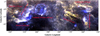 |
Fig. 1 Location of the California GMC with respect to other nearby molecular cloud complexes. The three-color RGB map was created using publicly available data: 850 μm (red) and 350 μm (green) from Planck imaging, and 100 μm (blue) from IRAS (Planck Collaboration XI 2014, Public Data Release 2). The distances of the molecular clouds indicated on the map were inferred from Gaia DR2 parallaxes (Zucker et al. 2019). |
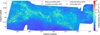 |
Fig. 2 Column density map of the California GMC at an angular resolution of 18.2″, derived from Herschel data with hires (see Sect. 2). The positions of the dense cores identified with getsf (see Sect. 3.2) are overlaid and shown as ellipses of various colors according to core type (blue for robust prestellar cores, blue and brown for candidate prestellar cores, orange for unbound starless cores). For easier visibility, the full axes of the ellipses have twice the actual Gaussian full width at half maximum (FWHM) sizes. Protostellar cores are marked with black pentagrams. |
2 Herschel data and derived column densities
The Herschel imaging observations of the California GMC (Harvey et al. 2013) were taken in parallel mode in the PACS 70 and 160 μm (Poglitsch et al. 2010) and SPIRE 250, 350, and 500 μm (Griffin et al. 2010) wavebands, with full width at half maximum (FWHM) beam sizes of 8.4, 13.5, 18.2, 24.9, and 36.3″, respectively, and a scanning speed of 60″s−1. The corresponding Herschel multiwavelength data were downloaded from the NASA/IPAC Infrared Science Archive1.
To create a column density map at 18.2″ resolution, we used the hires utility (Men’shchikov 2021b), an implementation within the getsf package of the multiresolution technique introduced by Palmeirim et al. (2013, see their Appendix A). The hires utility performs pixel-by-pixel fitting of the four Herschel images at 160, 250, 350, and 500 μm to derive dust temperature and column density images of the California GMC at various angular resolutions and uses the multi-scale differential approach of Palmeirim et al. (2013) to improve the resolution of the resulting map to 18.2″.
The derivation of reliable column densities and temperatures from Herschel data based on pixel-by-pixel fitting of the observed spectral energy distributions (SEDs) requires that the input images have accurate low-level intensities on large scales (also known as “zero levels”). Due to their finite sizes, the original Herschel maps usually do not have satisfactory zero levels and need to be corrected by adding appropriate zero-level offsets. The latter can be estimated by comparing smoothed versions of the Herschel images with corresponding low-resolution (5′) data from the Planck and IRAS all-sky surveys (cf. Bernard et al. 2010; Bracco et al. 2020). The estimated zero-level offsets for the California GMC at 160, 250, 350, and 500 μm are 4.7, 35.9, 17.8, and 5.8 MJy sr−1, respectively.
The observed images were reprojected to the same grid, covering a total area of 7° × 2.3° with a pixel size of 3″. The hires utility generated images of the H2 column density  and dust temperature Td at resolutions of 18.2, 24.9, and 36.3″ resolutions. In this process, a dust opacity law κλ = 0.1 × (λ/300 μm)−β cm2 g−1 with a fixed β = 2 (Roy et al. 2014) was assumed. The column density image at 18.2″ resolution (~0.04 pc at d = 470 pc) is instrumental to accurately detect and measure sources and filaments and reveals more details about the molecular cloud than the lower-resolution maps. The 18.2″ column density map (see Fig. 2) is publicly available in fits format from the CDS.
Having prepared the images, we applied the getsf source and filament extraction method (Men’shchikov 2021b) to separate the structural components of sources, filaments, and background and extract the sources and filaments in their respective images. The getsf extraction method is an improved version of its predecessors getsources, getfilaments, and getimages (Men’shchikov et al. 2012; Men’shchikov 2013, 2017). For a detailed benchmarking and comparisons of the new and old methods, the reader is referred to Men’shchikov (2021a).
3 Results and analysis
3.1 Mass distribution
The California GMC exhibits a hierarchical pattern, comprising a broad smooth background, web-like filamentary structures, and compact sources such as dense cores. The getsf extraction method, as described by Men’shchikov (2021b), segregates the structural components into their separate images. These separated components can be used quantitatively as they are guaranteed to reconstruct the original image through the addition of the components. Their respective masses can be estimated by summing up all pixel values in their individual column density maps:
 (1)
(1)
Here,  represents the mean molecular weight per H2 molecule, mH denotes the mass of a hydrogen atom, Δ denotes the pixel size, and
  corresponds to the column density of the given structural component at pixel i. The total mass of the California GMC within the Herschel-observed region (Fig. 2) is Mtot = 3.08 × 10⁴ M⊙. The resulting filamentary structures contain 6500 Μ⊙ (21% of Mtot), and the sources contain 550 M⊙ (1.8% of Mtot). The visual extinction (AV) is determined from the H2 column density using the relationship
  mag (Bohlin et al. 1978).
The probability density function of column density PDFN is shown in Fig. 3. The high-density tail of the PDFN exhibits a power-law shape suggestive of gravitational collapse (e.g., Federrath & Klessen 2013), with an exponent of −3.2, akin to the −2.9 value for Aquila (Könyves et al. 2015) but steeper than the −1.9 value for Orion Β (Schneider et al. 2013; Könyves et al. 2020). Notably, discernible source components emerge when AV > 4, becoming more pronounced at AV > 6. Defining dense gas as gas with 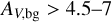 , the filament and source components correspond to 66–73% and 10–14% of the dense gas mass, respectively.
 |
Fig. 3 Column density probability distribution function (PDFN) obtained from the 18.2″ resolution image shown in Fig. 2, along with its structural components. For 2 ≤ Av ≤ 5, the PDFN follows a power law with an exponent of −3.2. It becomes slightly flatter for 5 ≤ Av ≤ 10, but its power-law exponent returns to −3.2 for Av > 10. |
3.2 Identification and analysis of dense cores
Following the standard approach introduced by Könyves et al. (2015) for identifying dense cores in the Herschel images of nearby clouds taken as part of the HGBS, we performed two sets of getsf extractions – tailored to starless cores (combining the 18.2″ column densities with 250, 350, and 500 μm images for source detection) and to protostellar cores (detecting them only in the 70 μm image), respectively. Measurements of detected sources were done in all images.
From the getsf extraction catalogs, we selected only those sources that met the standard HGBS criteria for core identification, based on column density detection, global detection significance, goodness, monochromatic detection significance, goodness, and signal-to-noise ratio (see Sect. 4.5 of Könyves et al. 2015). Such a selection is crucial for eliminating potential spurious detections, ensuring that only reliable and well-measurable sources are included. To further exclude extragalactic sources, we cross-matched the source positions with SIMBAD and the NASA/IPAC Extragalactic Database within a 6″ matching radius, which left us with 970 acceptable candidate cores. Following the standard approach, sources that were detected at 70 μm and were, at most, marginally resolved ( ), where A represents the major axis size at half-maximum and Β represents the minor axis size at half-maximum, and were not too elongated (A/Β < 1.5), were interpreted as candidate protostellar cores. In the California GMC, this resulted in a sample of 927 starless dense cores2 and 43 protostellar cores.
The FWHM size of a core was estimated as the geometric mean of its major and minor sizes, i.e.,  . We applied a simple Gaussian deconvolution method to remove the effect of the beam and recover a better estimate of the true source size from the observed S. Accordingly, the deconvolved size was estimated as
  , where Ο corresponds to the 18.2″ angular resolution of the column density map. The deconvolded sizes of sources with S close to Ο exhibit increased unreliability. To ensure reliable results and prevent unacceptably large deconvolution errors, we employed a resolvedness criterion and required S/O > 1.1 (see, e.g., Men’shchikov 2023). When S/O < 1.1, sources were considered partly resolved or unresolved, and assigned a deconvolved size equal to half of S. Figure 4 shows the mass versus size diagram for the starless cores identified in the California GMC. We use the thermal version of the critical Bonnor-Ebert mass, denoted as , to identify candidate prestellar cores. Prestellar cores are those starless cores which are dense enough to be self-gravitating, making them strong candidates for future protostar formation. is an approximation of the virial mass for an unmagnetized, thermal core, and can be expressed as follows:
  , where RBE is the Bonnor-Ebert radius, cs is the isothermal sound speed ~0.19 km s−1 for an ambient cloud temperature of 10 K, and G is the gravitational constant. We adopted Rdec = Sdec d as an estimate of RBE. Applying the criterion
  , we identified 209 starless sources as robust prestellar cores. Alternatively, applying the modified empirical formula αBE ≤ 10 × (O/S) based on our simulation tests (see Appendix A), we identified a larger sample of 405 candidate prestellar cores.
The differential CMFs derived for the samples of starless cores, candidate prestellar cores, and robust prestellar cores are displayed in Fig. 5. The three distributions merge at high masses (>1 M⊙) and are consistent with a power-law mass function ΔN/ΔlogM ∝ M−α with α= 1.4 ± 0.2, which agrees very well with the Salpeter power-law IMF (a = 1.35) (Salpeter 1955). A Kolmogorov-Smirnov (K-S) test on the cumulative core mass distribution N(> M) confirms that it is statistically indistinguishable from a power-law distribution above 1 M⊙ at a K-S significance level of >40% (equivalent to 0.9σ in Gaussian statistics). The error bar on the power-law index was estimated from the range of best-fit exponents for which the K-S significance level was larger than 5% (equivalent to 2σ in Gaussian statistics) when comparing the observed CMF with a power law above a minimum core mass in the range 1.0–1.4 M⊙.
Figure 6 shows the relationship between the median mass of prestellar cores and the local background level, which was estimated by subtracting the contribution of extracted sources from the original observed image while preserving the filament and large-scale background components. The two quantities exhibit a positive correlation, suggesting that more massive prestellar cores tend to form in denser parts of the ambient cloud (see Könyves et al. 2020; Shimajiri et al. 2019a for other examples of this trend).
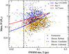 |
Fig. 4 Mass-size diagram for the cores identified in the California molecular cloud. “Extraction” represents the sizes measured directly on the 18.2″ column density map. “Decon. Robust”, “Decon. Candidate”, and “Decon. Unbound” represent the sizes of robust prestellar, candidate prestellar, and unbound starless cores, respectively, after deconvolution. The red solid line represents half of the mass of a thermally critical Bonnor-Ebert sphere (MBE/2) of radius R at a temperature of 10 K. The blue solid line marks the estimated threshold for selecting candidate prestellar cores. The dashed vertical line marks the 18.2″ beam size. |
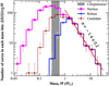 |
Fig. 5 Differential core mass function (ΔN/ΔlogM) for 927 starless cores (purple), 405 candidate prestellar cores and 209 robust prestellar cores. The vertical gray filled area at 0.45 ± 0.15 M⊙ denotes the estimated 90% completeness level for prestellar cores (see Appendix A). Error bars represent statistical uncertainties ( |

3.3 Analysis of the filamentary network
Filaments within molecular clouds are elongated and relatively dense structures that are commonly found throughout these clouds (cf. Men’shchikov et al. 2010; André 2017; Arzoumanian et al. 2019). They exhibit an intricate network-like morphology, with interconnecting structures that form complex patterns. The physical parameters of the whole network of filamentary structures characterize the extent to which its parent molecular cloud collapses from a diffuse state to a dense structure (cf. Ballesteros-Paredes et al. 2020). The genesis of filaments within molecular clouds is believed to be a result of several physical processes, including large-scale turbulence, magnetic fields, and gravitational instability (cf. André et al. 2014, and references therein). Filaments play a crucial role in facilitating the formation of dense cores by providing favorable conditions for the gravitational collapse of gas (cf. Li et al. 2023). Consequently, they serve as important nurseries for the birth of stars.
In the present work, filaments were detected as part of the same getsf extraction process that we used to identify candidate dense cores in the Herschel data (see Sect. 3.2). In our analysis, we chose a global skeleton, which traces filamentary structures on all transverse scales up to an angular diameter of 160″, i.e., approximately 0.4 pc, independently of the filament widths. The corresponding filamentary network is illustrated in Fig. 7, while a zoomed area of the detected filaments is presented in Fig. 8. The filament skeleton map is publicly available in fits format from the CDS.
While on large (>10pc) scales the California GMC appears to be a sheet-like 3D structure viewed almost edge on (Rezaei Kh. & Kainulainen 2022), the vast majority of the smaller-scale (≲lpc) filaments and cores identified here are unlikely to be predominantly elongated along the line of sight as (1) this is statistically improbable for a large number of randomly-oriented substructures embedded within a sheet-like cloud, and (2) several of our Herschel cores and filaments have been successfully observed and detected in dense gas tracers such as H13CO+(1−0) and N2H+(1−0) (Zhang et al. 2018; Chung et al. 2019), proving that they consist of dense ≳104 cm−3 gas as opposed to column density enhancements resulting from the accumulation of large amounts of low-density gas along the line of sight (cf. Li & Goldsmith 2012, for the example of the Taurus main filament).
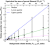 |
Fig. 6 Median candidate prestellar core mass plotted against background cloud column density (AV units) is shown by the black triangles. The error bars represent the inter-quartile range of observed masses within each bin. The green dashed line depicts a linear fit to the median masses as a function of AV,bg, given by Mmed ∝ (0.2 ± 0.02) × AV,bg. The blue dash-dotted line corresponds to a linear fit to the upper quartiles of median observed masses, while the magenta dotted line represents a linear fit to the lower quartiles. |
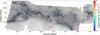 |
Fig. 7 Global filament network including all transverse angular scales up to ±80″ across the filament spines. A thick skeleton mask with a fixed line width of about 4 pixels (12″), color-coded as shown in the bar on the right, is overlaid on the original column density image shown as a grayscale background. Map values at the skeleton pixels correspond to background- and source-subtracted column densities on the filament crests. |
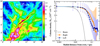 |
Fig. 8 Close-up view of the filament network (left) and example of a filament radial profile (right). Left: skeletons of several filaments depicted as grey solid curves and traced within a 20′ × 20′ subfield of the column density image at 18.2″ resolution. The black curve represents the skeleton of the filament whose radial profile is displayed in the right panel. Right: median one-sided column density profiles measured on both the left (purple solid line) and right (blue) sides of the filament, with the black dashed curve representing the beam profile. The median half maximum width measured on the left (north-east) side is 0.13 pc, that on the right (south-west) side is 0.17 pc, and the mean is 0.15 pc. |
3.3.1 Measurement and statistics of extracted filaments
Filamentary structures are more difficult to define and analyze than dense cores. In contrast to cores, observed filaments often have complex shapes, variable intensity along their crests (cf. Roy et al. 2015), and are frequently interconnected with each other (e.g., Men’shchikov 2021b). It is often unclear where a filament starts, where it ends, and which branch of the interconnected filamentary network describes a real physical filament. To enable an accurate analysis of the observations, it is necessary to decompose the complex filamentary pattern seen in the Herschel images into simpler entities. The approach employed by getsf is to break all branches of a filament network into simple non-branching structures, hereafter referred to as elementary skeletons, to aid in the selection of individual filamentary structures for which accurate measurements are possible (Men’shchikov 2021b).
Properties of the filamentary network in the California GMC were measured in the column density map of the filamentary component at angular resolution Ο = 18.2″, free from the contributions of compact sources and large-scale backgrounds. The measurements were done with fmeasure, a utility of the getsf software. Both sides of the filaments were measured separately. For the purpose of estimating local filament properties, we also truncated each filament into segments of 0.1 pc length, a size scale comparable to the typical half-power width of both HGBS and California filaments (see below and Arzoumanian et al. 2019). Such filament segments are referred to as “chunks” in the following (see also Sect. 3.3.3).
Some filaments may be contaminated or blended with an adjacent filament; as a result, the width on one side or sometimes even both sides cannot be effectively measured. An effective measurement on one side is determined by two criteria: the profile falls below the half power maximum, and the width on this side is less than twice the width on the other side. When estimating a filament’s width, only the side(s) that could be effectively measured was considered. If both sides were effectively measured, the width W was estimated as the mean of WA and WB, W = (WA + WB)/2, where WA represents the filament’s median half-maximum width measured on side A and WB is the measurement on side B. These widths are half-power diameters estimated by getsf directly from the profiles without any (Gaussian or Plummer) fitting, and are comparable to the “half diameters” hd discussed by Arzoumanian et al. (2019). The distribution of observed widths for the filaments identified with getsf in California is shown in Fig. 9a.
The column density contrast (C) of a filament may be defined as  , where
  represents the median column density along the crest of the filament and
  denotes the background column density of the filament (cf. Arzoumanian et al. 2019). Higher-contrast filaments are easier to measure accurately due to a higher signal-to-noise ratio, since high contrast reduces noise impact and provides a clearer distinction from the background and other structures. The median value of Wobs for filament skeletons with C > 0.4 (0.19 pc) deviates only slightly by 0.01 pc from that for skeletons with C > 0.2 (0.18 pc). Similarly, for filament “chunks”, the median Wobs with C > 0.4 (0.18 pc) also shows a 0.01 pc deviation from that for chunks with C > 0.2 (0.17 pc). The agreement between the median filament widths obtained for C > 0.4 and C > 0.2 confirms the robustness of our measurements across different column density contrasts. The Wobs widths found here for the California GMC filaments are consistent within better than a factor of 2 with the typical inner width of ~0.1 pc measured for nearby (d < 0.5 kpc) molecular filaments with Herschel (Arzoumanian et al. 2011, 2019), especially if finite-resolution effects and the relatively large distance of the California GMC (see André et al. 2022) are taken into account. Note that we do not try to deconvolve the measured filament widths from the telescope beam here, because the simple Gaussian deconvolution approach has been shown to be highly inaccurate, especially for filaments with power-law intensity profiles in the presence of significant background fluctuations (André et al. 2022; Men’shchikov 2023).
The distribution of median temperatures along the filament crests is shown in Fig. 9b. When C > 0.4, skeletons and chunks have median dust temperatures of 15.2 K. The median dust temperatures for skeletons and chunks with C > 0.2 are only slightly warmer, at 15.5 and 15.4 K, respectively.
The distribution of measured logarithmic slopes s for all filament column density profiles is presented in Fig. 9c, where the slope s is defined as  (dimensionless) and measures how fast column density drops with radial distance from each filament’s crest. Note that this drop is often quantified in terms of the logarithmic slope −p = s − 1 of the underlying density profile, e.g., when Plummer-like model profiles are fitted to the data (e.g., Arzoumanian et al. 2011, 2019). The magnitude |s| of the logarithmic slope directly controls the prominence of filament wings and the resemblance of the filament profile to a Gaussian shape. A higher |s| (or p) value indicates less prominent filament wings and a filament profile that more closely resembles a Gaussian curve. The distribution of s slopes has a peak at −1, and a median value at about −1.45 for filament skeletons and −1.35 for filament chunks. Accordingly, the p-index has a mode value of +2, and a median value of +2.45 for skeletons and +2.35 for chunks. Tests on high-contrast filaments (Contrast: C > 1 and aspect ratio: AR > 4) confirm that the logarithmic slopes derived by getsf (without Plummer fitting) are consistent with the p-index that would be derived by Plummer fitting. Indeed, our results are in good agreement with the p-index slopes found by Arzoumanian et al. (2019) for nearby HGBS filaments using Plummer model fits.
Filament crest column densities and line masses are positively correlated with filament contrasts, as shown in Fig. 10a,b. This correlation indicates that higher-contrast filaments generally have higher column densities. The average line mass of a filament, denoted as  , was estimated as
  , where Mfil represents the filament mass, and Lfil corresponds to the filament length. The filament mass, Mfil, was obtained by integrating column density over the entire footprint of the filament, while the length Lfil was estimated from the length of the getsf skeleton.
  represents the line mass estimated from the integration of the median column density profile.
  is positively correlated with
  , as shown in Fig. 10c. However,
  tends to be slightly higher than
  . For high-contrast filaments (C > 0.4),
  appears to be a slightly better estimator of filament line mass than
  (cf. Appendix B).
Higher line-mass filaments tend to have lower dust temperatures as shown in Fig. 10d. As the density of a filament increases, resulting in a higher line mass, the filament becomes more effectively shielded against ambient radiation, leading to a decrease in filament dust temperature.
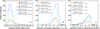 |
Fig. 9 Distributions of widths, dust temperatures, and radial density gradients for filament skeletons and chunks (with C > 0.2 and C > 0.4). (a) Distribution of measured FWHM widths. (b) Distribution of median dust temperatures measured on filament crests. (c) Histogram of logarithmic slopes s for the column density profiles of all measured filaments. (If both sides of a filament were effectively measured, the histogram count was incremented by 2; if only one side was measured, the histogram count was incremented by 1; if neither side could be measured, the histogram count was not incremented.) The median and peak values of each parameter are provided in the legend of the corresponding panel. |
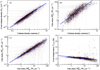 |
Fig. 10 Correlations between filament properties, (a) Filament crest column density against column density contrast. The blue solid line is the fit: |


3.3.2 Relation between filaments and cores
Filament line masses are known to vary along the filament crests (cf. Roy et al. 2015). Here, the line masses were estimated at each sampling point along the crests. For each core, the shortest separation between core center and the local network of supercritical filamentary structures was calculated. As shown in Fig. 11, our observations reveal that 82% of candidate prestellar cores and 90% of robust prestellar cores are positioned within 0.1 pc of the nearest supercritical filament. In contrast, only approximately 41% of unbound starless cores are situated within 0.1 pc of the nearest supercritical filament. These results are consistent with the findings of Könyves et al. (2020) and Ladjelate et al. (2020), and support the hypothesis that filamentary structures act as pathways for the accumulation of gas and dust, leading to supercritical fragmentation and the subsequent formation of gravitationally bound cores. A majority (~60%) of unbound starless cores and a small (~ 10–15%) fraction of prestellar cores are located far (~ 0.1 pc) from any supercritical filament, making up the secondary peak in the core-to-filament separation plot of Fig. 11. The nature of the cores in this second peak is not completely clear. Most of the unbound cores may never get massive enough to collapse and form stars before dispersing and may thus be “failed cores” (cf. Vázquez-Semadeni et al. 2005). On the other hand, the few candidate prestellar cores populating the second peak in Fig. 11 may be the progenitors of a small fraction of protostars that do not form in filaments.
 |
Fig. 11 Spatial relationship between extracted cores and supercritical filamentary structures, displayed as an histogram of separations between core centers and the nearest supercritical filamentary structures. |
3.3.3 Line mass function of California filaments
Background and noise fluctuations in observed images can easily break a continuous filament into multiple shorter filaments. As a result, when estimating integral quantities, such as the filament mass and length, the presence of unrelated fluctuations and the relative brightness (density) of the filament can introduce inaccuracies. Consequently, the physical conditions required for the formation of prestellar cores, particularly the volume densities, can vary along the filaments. This variability in physical conditions poses challenges when attempting to utilize the integral properties of filaments in studies related to star formation. However, it is not crucial to accurately determine the true integral properties of filaments. Instead, what matters more for star formation studies are the local properties of filaments in the immediate vicinity of the locations where appropriate physical conditions exist for the growth of prestellar cores.
Long filaments often exhibit significant variations in their local column densities and widths along their crests, which correspond to variations in their line masses denoted as Mline(l) (Roy et al. 2015), where l represents the position along the skeleton of a filament. We employed the fmeasure routine from the getsf software to trace each filament skeleton and determine the coordinates of all its pixels. To enhance the smoothness of the skeleton representation, getsf averages the coordinates of the pixels of a given skeleton over a seven-pixel window. This averaging process yields high-resolution coordinates for each point along the skeleton. Next, utilizing these high-resolution coordinates, each filament was truncated into pieces of 0.1 pc length, which is comparable to the typical half-maximum width of both HGBS and California filaments (see Arzoumanian et al. 2019 and Sect. 3.3.1). This truncation results in the creation of equally-spaced filament segments referred to as “chunks” here. Consequently, a filament network composed of individual 0.1 pc chunk units is established.
The Mline(s) values measured for each of the 0.1 pc chunks were used to construct the filament line mass function (FLMF) shown in Fig. 12 as blue and green histograms. We stress that since the 0.1 pc length of each filament chunk significantly exceeds the linear resolution of our column density map (18.2″ or ~0.04pc at d = 470 pc), the measured Mline(s) values are mutually independent. As described in Appendix B, the derived sample of filaments is deemed to be 80% complete for Mline > 10 M⊙ pc−1. Figure 12 shows that, in this regime of high line masses, Mline > 10 M⊙ pc−1, the FLMF is consistent with a power law:  .
.
A Kolmogorov-Smirnov (K-S) test on the cumulative line mass distribution N(>Mline) confirms that it is statistically indistinguishable from a power-law distribution  at the K-S significance level of 10% (equivalent to 1.6σ in Gaussian statistics) in the regime of thermally supercritical filaments, i.e., for Mline > 16 M⊙ pc−1. The error bar on the power-law index was estimated from the range of best-fit exponents for which the K-S significance level was larger than 5% (equivalent to 2σ in Gaussian statistics). Comparing the best-fit power laws to the FLMF observed above a minimum Mline value in the range from 10 to 25 M⊙ pc−1, we conclude that the power-law index of the FLMF is 1.5 ± 0.2 in the regime of high line masses. For comparison, each filament was also truncated into pieces of 0.2 pc in length, generating a filament network consisting of 0.2 pc chunks. The corresponding FLMF is also displayed in Fig. 12 as purple and orange dashed histograms. The latter is essentially identical to the 0.1 pc chunk FLMF for line masses >20 M⊙ pc−1.
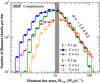 |
Fig. 12 Filament line mass function (FLMF, ΔN/ΔlogMline), derived from the sample of filament chunks in the California GMC. The error bars represent statistical uncertainties ( |

4 Discussion: Connecting the FLMF and the CMF
The shape of the California FLMF found in Sect 3.3.3 and shown in Fig. 12 is consistent with the Salpeter (1955) power-law IMF at the high-mass end. This contrasts with the mass function of molecular clouds and massive clumps within clouds, which is known to be significantly shallower than the Salpeter IMF, scaling as  (e.g., Solomon et al. 1987; Lada et al. 1991; Blitz 1993; Ellsworth-Bowers et al. 2015; Rice et al. 2016). The finding of Sect 3.3.3 strongly supports the existence of a connection between the FLMF and the CMF/IMF, as proposed by André et al. (2019) from an analysis of about 600 filaments in 8 nearby clouds covered by the HGBS (cf. Arzoumanian et al. 2019). Our present result shows that this connection holds at the level of an individual cloud, namely California. Moreover, the FLMF derived by André et al. (2019) was a distribution of mean line masses averaged along the length of each sampled filament, while the FLMF shown here in Fig. 12 is a distribution of local line masses for a complete, homogeneous sample of filaments in the same cloud. Since it is the local line mass of a filament which defines its ability to fragment at a particular location along its spine and not the average line mass of the filament (cf. Pineda et al. 2023, and references therein), the connection found here is more direct and provides tighter constraints on the origin of the CMF/IMF. Combining their result on the FLMF of HGBS filaments with the trend that higher-line-mass filaments tend to host more massive cores (see Shimajiri et al. 2019a; Könyves et al. 2020, and Fig. 6 here), André et al. (2019) proposed an empirical model for the origin of the CMF/IMF in filaments, whereby the global prestellar CMF - and by extension the global stellar IMF - arises from the superposition of the CMFs generated by individual filaments (see also Lee et al. 2017). Based on average line masses, the model had to assume that HGBS filaments have fixed, typical lengths of ~0.55 pc and uniform line masses along their lengths, which is obviously only a first order approximation. The result reported here allows us to simplify and improve this model by dropping the artificial assumptions of constant filament length and uniform line mass along each spine.
Briefly, our revised model of the CMF may be summarized as follows (see André et al. 2019 for further details). Denoting by  the differential CMF per unit log mass in a filament of line mass Milne (where m represents core mass), and by g(Milne) = dN/dlog Milne the differential FLMF per unit log line mass, the model posits that, at least in a statistical sense, the global prestellar CMF per unit log mass ξ(m) = dNtot/d log m in a molecular cloud corresponds to a weighted integration over line mass of the CMFs generated by the individual filaments present in the cloud3:
 (2)
(2)
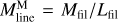
where w(Mline) ∝ CFE(Mline) × Mline × L represents the relative weight4 of a filament segment of length L (here L = 0.1 pc or L = 0.2 pc) as a function of Mline, and CFE(Mline) = Mcores/(Mline L) is the average prestellar core formation efficiency in a filament of line mass Mline. Based on Fig. 13 and the observational findings of Könyves et al. (2015), we adopt a dependence of CFE on Mline similar to André et al. (2019):
![Mathematical equation: ${\mathop{\rm CFE}\nolimits} \left( {{M_{{\rm{line }}}}} \right) = {{\mathop{\rm CFE}\nolimits} _{\max }}\left[ {1 - \exp \left( {{1 \over 4} - {{4{M_{{\rm{line }}}}} \over {3{M_{{\rm{line,crit }}}}}}} \right)} \right],$](/articles/aa/full_html/2024/09/aa49853-24/aa49853-24-eq44.png) (3)
(3)
with CFEmax = 30%. This “smooth step” functional form for CFE(Mline) is such that the prestellar core formation efficiency in each filament asymptotically approaches CFEmax = 30% for Miine > Mline,crit/2 and quickly drops to CFE(Mline) = 0 for Mline < Mline,crit/2 (see green curve and magenta histogram in Fig. 13). It provides a good fit to the core formation efficiency measurements in California (see Fig. 13), separating a regime with no core/star formation in thermally subcritical filaments from a regime with an asymptotic core formation efficiency of ~30% in thermally supercritical filaments. Likewise, based on the findings of Shimajiri et al. (2019a, 2023) and Könyves et al. (2020) and following André et al. (2019), we assume that the CMF produced by an individual filament,  , follows a log-normal distribution of variance
  centered on the effective Bonnor-Ebert (or Jeans) mass
  in that filament, where cs,eff is the one-dimensional gas velocity dispersion or effective sound speed and Σfil ∝ Mline is the local gas surface density in the filament. Recalling that thermally supercritical filaments are observed to be virialized with
  (Arzoumanian et al. 2013, see also Fiege & Pudritz 2000), we see that MBE,eff ∝ Mline. Thus, the model assumes that the location of the CMF peak in each filament scales with Mline. In other words, higher-mass cores form in more massive filaments, a trend suggested by observations (Shimajiri et al. 2019a, 2023, and Fig. 6 here). To reproduce the increasing dispersion of core masses with background column density (Fig. 6), we adjusted the variances of the lognormal distributions
  in the model as follows:
 ![Mathematical equation: $\sigma _{{M_{{\rm{line }}}}}^2 = {0.3^2} + 0.2{\left[ {\log \left( {{M_{{\rm{BE}},{\rm{eff}}}}/{M_{{\rm{BE}},{\rm{th}}}}} \right)} \right]^2}$](/articles/aa/full_html/2024/09/aa49853-24/aa49853-24-eq50.png) . The prestellar CMFs predicted by this empirical model in various column density regimes are shown in Fig. 14. It can be seen that the model reproduces both the global CMF and the variations of the CMF with background column density reasonably well.
. The prestellar CMFs predicted by this empirical model in various column density regimes are shown in Fig. 14. It can be seen that the model reproduces both the global CMF and the variations of the CMF with background column density reasonably well.
Our measurements of the FLMF and prestellar CMF in the California GMC (Sect. 3), coupled with the analysis and toy model presented in this section, therefore bolster the notion that the prestellar CMF – and by extension the stellar IMF itself – may be at least partly inherited from the FLMF. Interestingly, the numerical study by Abe et al. (2021) suggests that only specific theoretical scenarios for filament formation and evolution, such as the oblique MHD shock compression mechanism (Inoue & Fukui 2013), can account for a tight connection between the FLMF and the CMF/IMF, while other mechanisms, such as turbulence-induced shear or collision of turbulent shock waves, either do not produce massive enough filaments or do not lead to line mass functions resembling the Salpeter IMF at the high-mass end. The global hierarchical collapse (GHC) model advocated by Vâzquez-Semadeni et al. (2019) may potentially explain the link between the slope of the FLMF and the slope of the CMF/IMF since cores continuously accrete from their parent filamentary structures and protostars similarly accrete from their parent cores in this picture. However, the difference in slope between the cloud/clump mass function and the slope of the FLMF is difficult to understand in the GHC framework since dense filaments are also observed to accrete from their parent clouds/clumps (e.g., Palmeirim et al. 2013; Kirk et al. 2013; Shimajiri et al. 2019b). In any event, the FLMF appears to be a key feature of the population of dense molecular filaments that closely relates to the origin of stellar masses and deserves further attention from theorists of the cold ISM.
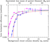 |
Fig. 13 Differential core formation efficiency (CFE) in the California GMC as a function of background cloud column density (blue histogram with error bars) and parent filament column density (magenta histogram), both expressed in AV units. The CFE values were obtained by dividing the mass in the form of candidate prestellar cores in a given column density bin by the cloud mass (blue histogram) or estimated filament mass (magenta histogram) in the same column density bin. The upper x-axis provides a rough estimate of the equivalent filament line mass assuming the parent filament of each core has an effective width 0.18 pc (corresponding to the median observed filament width – see Sect. 3.3.1). The vertical dashed line marks the position of the thermally critical line mass Mline,crit ~ 16 M⊙pc−1, corresponding to AV,bg ~ 4.5. The red and green curves show simple fits to the blue and magenta histograms, respectively, with a smooth step function of the form CFE(AV) = CFEmax[1 − exp(a × AV + b)], with CFEmax ≈ 30%. For the blue distribution, α = −0.16 and b = 0.4; for the magenta distribution, α = −0.28 and b = 0.25. |
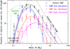 |
Fig. 14 Comparison of the prestellar CMFs (in ΔN/ΔlogM format) expected in the toy model described in André et al. (2019) and in the text (solid and dashed curves) with the observed prestellar CMFs observed in the California GMC (data points and histograms) at low column densities ( |


5 Conclusions
We used Herschel SPIRE/PACS parallel-mode maps in five photometric bands between 70 and 500 μm to study dense cores and filamentary structures in the California molecular cloud, employing the getsf algorithm for source and structure identification. The physical properties of these cores and filaments were analyzed, and the relationship between the FLMF and the CMF discussed. Our main findings and conclusions can be summarized as follows:
The structure of the California GMC is hierarchical in nature, whereby the majority (~80%) of the cloud’s overall mass is distributed in a large-scale, low-density background, ~20% of the mass is concentrated in the form of filamentary structures, and only ~2% of the mass is in the form of compact sources such as dense cores.
We identified 43 protostellar cores and 927 starless dense cores, 405 of which were classified as candidate prestellar cores, including 209 robust prestellar cores. For core masses M > 1 M⊙, the prestellar CMF is well fit by a power law ΔN/ΔlogM ∝ M−1.4±0.2, in excellent agreement with the Salpeter power-law IMF.
A vastmajority of robust (90%) and candidate (82%) prestellar cores are located within 0.1 pc of their nearest thermally supercritical filament. The mass of each prestellar core appears to be positively correlated with the column density of the local background, itself dominated by the parent filament. These findings highlight the tight connection between the cloud’s filamentary structure and the distribution of prestellar core masses.
The distribution of measured FWHM widths for the California filaments has a median (undeconvolved) value of 0.18 pc using column density data on either side of the filament crests. Given the distance of the California GMC and the resolution of the Herschel column density data, this is consistent with intrinsic filament widths close to ~0.1 pc on average, as reported earlier for other nearby clouds. The derived filament column density profiles have a most frequent logarithmic slope of about −1.1 and a median logarithmic slope of about −1.4, corresponding to logarithmic slopes of −2.1 and −2.4 for the underlying density profiles, respectively. The median dust temperature along the filament crests is ~15 K.
The sample of analyzed filaments is estimated to be 80% complete for line masses above ~10 M⊙ pc−1. We derived for the first time the distribution of local masses per unit length for such a complete sample of filamentary structures and found that the corresponding FLMF is consistent with a power-law distribution,
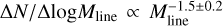 , for line masses greater than 10 M⊙ pc−1. This is similar to the Salpeter power-law IMF, supporting the notion that both the prestellar CMF and the stellar IMF may be partly inherited from the FLMF.
Using an improved toy model for the prestellar CMF in filaments that eliminates assumptions of constant filament length and uniform line mass, we established a more direct link between the FLMF and the CMF/IMF. In this toy model, the global prestellar CMF in a molecular cloud corresponds to a weighted integration of the CMFs generated by individual filaments within the cloud. Overall, our study highlights the role of molecular filaments in shaping the formation and mass distribution of newly born stars.
Acknowledgements
This work started in 2018 in the HGBS group of the Astrophysics Department (DAp/AIM) at CEA Paris-Saclay. After returning to China in 2020, G.-Y.Z continued to carry out this work at the China-Argentina Cooperation Station of NAOC/CAS. G.-Y.Z acknowledges support from a Chinese Government Scholarship (No. 201804910583), the China Postdoctoral Science Foundation (No. 2021T140672), and the National Natural Science foundation of China (No. U2031118). This work also received support from the Key Project of International Cooperation of the Ministry of Science and Technology of China under grant number 2010DFA02710, as well as from the National Natural Science Foundation of China under grants 11503035, 11573036, 11373009, 11433008, 11403040, and 11403041. P.A. acknowledges support from CNES, “Ile de France” regional funding (DIM-ACAV+ Program), and the French national programs of CNRS/INSU on stellar and ISM physics (PNPS and PCMI). We thank the anonymous referee for their positive feedback and insightful comments.
Appendix A Completeness for prestellar cores
In our investigation of the completeness of prestellar core extraction in the California cloud, we followed a methodology similar to that employed by Könyves et al. (2015) in their study of prestellar cores in Aquila (see Appendix B.2 of their paper). Our approach involved simulating prestellar cores within Herschel images using radiative transfer models of critical Bonnor-Ebert spheres with well-defined physical properties. These synthetic model cores were incorporated into source-free background images derived from actual observations, effectively generating synthetic Herschel and column density images that reflected the core characteristics in the California cloud.
The specific details of our simulation are as follows. We generated synthetic images at Herschel wavelengths (70, 160, 250, 350, and 500 μm) with an angular resolution that matched the observed values of 8.4, 13.5, 18.2, 24.9, and 36.3″. Additionally, we produced a column density map at an 18.2″ resolution using the simulated images across the 160 to 500 μm range. In total, we included 1041 synthetic prestellar cores within the simulation. We used a background column density threshold of 3 × 1021 cm−2 for simulated sources. Additionally, column density levels were spaced by a factor of 1.3, with considerations for ratios between model and background column densities to ensure reliable placement of model cores. We did not simulate any protostars, focusing solely on prestellar cores. We divided the mass distribution into 25 discrete mass bins. The core mass function of the model followed ΔN/ΔlogM ∝ M−0.7, with a lower mass limit of 0.04 M⊙ and an upper mass limit of 20 M⊙. To optimize the placement of model cores, we sorted them based on their radii. Randomization was employed for cores with masses exceeding a specified limit of 0.5 M⊙. Additionally, a maximum beam size of 24.9″ was used to control any potential overlap between sources.
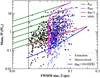 |
Fig. A.1 Mass–size diagram of the cores detected in the simulated Herschel images. The red line represents half of the critical Bonnor-Ebert mass (MBE/2) at 10 K as a function of radius. The blue line shows the empirical threshold used to select candidate prestellar cores in Sect. 3.2 (cf. Fig. 4), which captures 95% of the synthetic prestellar cores in the simulation. The curves labeled RBES (in magenta) show the mass vs. radius relations for the convolved model cores, while the lines labeled RAS (in green) represent the true mass vs. radius relations of the models. The black dashed vertical line shows the minimum derived model size (MMS) used when applying simple Gaussian deconvolution to the simulated extraction results (see Sect. 3.2). |
We applied the getsf method to extract the model cores within these synthetic images, and we employed the same approach as outlined in Sect. 3.2 to select reliable candidate cores. As our simulations were conducted using prestellar parameters, the model cores were exclusively self-gravitating prestellar cores. Comparison with the extracted sources shows that the default selection criterion to select prestellar cores,  , is overly strict, as it only selects ~70% of the model prestellar cores in our simulated images (as shown in Fig. A.1). In the previous study by Könyves et al. (2015), an empirical formula for selecting candidate prestellar cores was introduced: αBE ≤ 5 × (O/S)0.4. We have adjusted this formula based on our present simulation results to suit the detection outcomes for the California cloud. The modified empirical formula is as follows: αBE ≤ 10 × (O/S). This revised formula, shown as a blue curve in Fig. A.1, successfully identifies 95% of prestellar cores in our simulation detection results.
The core masses discussed in the present paper were derived via SED fitting of the background-subtracted total fluxes measured toward each core. In the literature, another, simpler method has also been used to gauge core masses, by integrating column density over the footprint of each core in the  map derived from Herschel data and subtracting the estimated
  backgound. For this reason, we tested both approaches using our simulation. Figure A.2c clearly shows that SED-derived masses tend to be closer to the true values than
  -based masses. As expected, SED-derived masses become more accurate for stronger, more massive cores. Above ~ 0.5 M⊙, the median ratio of SED-derived to true core mass is about 20% on average, indicating a slight overestimation of core masses. In comparison,
  -based masses underestimate true masses by approximately 45% on average.
In Fig. A.3a, we assess prestellar core completeness by comparing the number of detected cores within each mass bin to the true number of model cores. As core mass increases, completeness improves. For true core masses exceeding 0.25 M⊙, the completeness level exceeds 90%, fluctuating between 80% and 100% thereafter. Figure A.3b presents the recovered CMF from simulated source extractions, when cores are binned using true masses. The recovered CMF matches well the input mass function (ΔN/ΔlogM ∝ M−0.7) of the model cores above 0.25 M⊙, while the drop below this level is due to significant incompleteness of core detections at lower masses, as shown in Fig. A.3a. Since the derived core masses are typically overestimated by 20%, this suggests that the completeness level is ~ 0.25 × 1.2 = 0.3 M⊙ in observed core mass. On the other hand, when cores are binned in terms of SED-derived mass as opposed to true mass, the measured CMF (shown in Fig. A.3c) is consistent with the input power-law mass function only above ~0.6 M⊙, suggesting that good completeness is only achieved above ~0.6 M⊙ in observed core mass. In summary, we conservatively estimate that the actual 90% completeness level of our Herschel census of prestellar cores in California is in the range of ~0.3−0.6 M⊙ or 0.45 ± 0.15 M⊙ in derived core mass.
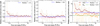 |
Fig. A.2 Accuracy of core measurements according to the simulations, a) Measured FWHM radius versus model radius (RBES)- Perfect core radius estimates would lie on the horizontal magenta dotted line. The horizontal solid line marks the median ratio value for cores with M > 0.25 M⊙. b) SED-derived temperature against true dust temperature of the model, c) SED-derived and |

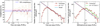 |
Fig. A.3 Tests for estimating the completeness of core extractions based on the simulations, a) Fraction of recovered synthetic cores as a function of true core mass. The error bars represent the ±1σ deviation within each mass bin and the magenta dotted line marks 100% completeness, b) Recovered CMF after extracting the simulated cores and binning the results according to true core mass, c) Recovered CMF after extracting the simulated cores and binning the results according to SED-derived mass. |
Appendix B Completeness for extracted filaments
To assess the completeness of the extracted filamentary structures, a series of additional simulated images were generated. This process involved the insertion of synthetic filamentary structures with known parameters into a synthetic background image. The synthetic background image, depicted in Fig. B.1b, was created by superimposing synthetic cirrus cloud fluctuations spanning all spatial scales onto a smooth background (Fig. B.1a) generated by getsf.
To ensure that the simulated filaments closely resembled the lengths and curvatures of the observed filaments, we used the skeletons of the X-shaped nebula region, which were obtained during our filament extraction process in the California cloud (see Zhang et al. 2020). We distributed these skeletons at ten locations within the image area, allowing for rotations of 90° or 180° and/or mirroring, as depicted in Fig. B.1c. Subsequently, we transformed these skeletons into simulated filaments using the modfits utility, an integral component of the getsf extraction software (Men’shchikov 2021b). The transformation was accomplished by applying a prescribed Moffat (Plummer) profile, represented by the equation:
 (B.1)
(B.1)
where θ is the angular distance from the skeleton, W is the filament full width at half maximum, s < 0 is the power-law exponent of the column density profile at large radii, and N0 is the crest column density. This function has an almost flat, Gaussian inner profile at θ < W/2 that transforms into a power-law profile 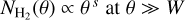 . We parameterized the filament strengths by the contrast C = N0/NB with respect to the background value. By adjusting the values of C and W, we were able to evaluate the ability of getsf to detect weaker or wider filaments, thereby allowing us to assess the extraction completeness limits.
As an illustration, Fig. B.1d shows the model filaments (for C = 1, W = 0.15 pc, and s = −1.5) and Fig. B.1e displays the complete simulated image. To investigate how the filament detectability depends on contrast and width, we created a set of synthetic images with different values of C (0.1, 0.2, 0.3, 0.4, 0.5, 0.6, 0.8, 1, 2, 4) and W (0.05, 0.08, 0.1, 0.13, 0.15, 0.18, 0.2, 0.3, 0.4 pc), while keeping s = −1.5 constant, similar to the average logarithmic slope estimated in the real California data (Fig. 9). The model filaments were extracted independently in each image, adopting the same value for the getsf maximum width parameter as used in the extractions performed with the observations (cf. Sect. 3.3). This ensures that the simulations described here accurately reflect our analysis of real data.
For each simulated filament, we used well-defined parameters for the width, contrast, and power law exponent of the filament profile. These fixed parameters represent the true parameters of the simulated filament. However, the intrinsic line mass of each simulated filament is not accurately known and needs to be calibrated. To do so, we used fmeasure to measure each simulated filament in the absence of background fluctuations and obtain its intrinsic line mass. The filaments display curvature and the images contain more than one filament. To address concerns related to self-blending and overlap with other filaments, we artificially straightened the filaments within the images, thereby isolating the filaments from one another. An example of such a straightened, single filament is illustrated in Fig. B.2. This isolated filament has no background, and its boundaries can extend indefinitely. To mitigate this issue, the fmeasure sets an arbitrary boundary where the density is 100 times lower than that of the crest.
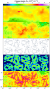 |
Fig. B.1 Simulated 3.3° × 1.1° column density image of a filamentary cloud at 18.2″ resolution: (a) large-scale background produced by the getsf analysis of the California data; (b) synthetic background cloud; (c) skeletons detected by getsf in the X-shaped nebula; (d) simulated filaments; (e) complete synthetic image of the simulated filamentary cloud. |
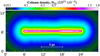 |
Fig. B.2 Illustrative example of an artificially straightened filament with a width of W = 0.1 pc, a contrast of C = 1, and a power-law exponent of s = −1.5. |
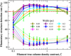 |
Fig. B.3 Fraction of recovered model filaments with various intrinsic widths (solid lines) as a function of column density contrast. The red dashed horizontal line marks an 80% completeness level. The dotted lines represent the fraction of spurious filaments. |
Analyzing the extraction results, we matched the filament skeletons detected in the simulated images with the true model skeletons. The adopted matching radius was  , where Ο represents the telescope resolution (~ 0.04 pc) and W is true FWHM size of the model filament. The resulting filament detection rates are shown in Fig. B.3 for a wide range of model filament contrasts. The detection rate is lower for wider filaments, because the wider power-law wings of such filaments imply similarly wider footprints and higher inaccuracies in their background subtraction. For model filaments with W ≲ 0.15 pc, W ≲ 0.18 pc, and W = 0.2 pc, the detection rate exceeds 90% at C ≳ 0.2, C ≳ 0.3, and C ≳ 0.4, respectively. For wider model filaments with W = 0.3 pc and W = 0.4 pc, the detection rate is higher than 80% when C ≳ 0.3 and C > 0.4, respectively. Based on the upper envelope of the relation between filament line mass and column density contrast shown in Fig. 10b, we therefore estimate that the 80% detection completeness level of our filament sample is at ~10M⊙pc−1 in terms of derived
  values. Since
  is typically underestimated by 30 ± 20% when C > 0.4 (see below), this completeness level corresponds to ~ 13 M⊙pc−1 in terms of intrinsic filament line mass.
The simulations described in this Appendix were are also used to assess the accuracy of derived filament properties. To do so, we used the input model skeletons to measure the filament properties in the filament component map derived from the simulated image, and then compared the measurement results with the true properties to evaluate the measurement accuracy of each property. We define the measurement accuracy RD of a parameter X as the relative difference between the measured value (Xm) and the true value (Xt) of the parameter, i.e.,  . Figure B.4 shows the measurement accuracy of filament widths as a function of filament contrast for several intrinsic values of the filament width. It can be seen that, at low contrasts ~0.1, the filament width estimates can be quite inaccurate. However, as the contrast increases, the measurement results progressively converge toward the true widths of the model filaments. At filament contrasts higher than 0.4, the average measurement accuracies are 0.73, 0.34, 0.23, 0.12, 0.08, 0.02, -0.01, -0.12, and 0.1 for filament widths of 0.05, 0.08, 0.1, 0.13, 0.15, 0.18, 0.2, 0.3, and 0.4 pc, respectively. For model filaments with intrinsic widths of 0.18 and 0.2 pc, the measurements are very good with errors of less than 2%. For intrinsic widths from 0.13 to 0.4 pc, the width estimates remain very accurate with errors of less than 10%. For intrinsic widths of 0.08 and 0.1 pc, the measurement errors range from 20 to 35%. For model filaments with intrinsic widths of 0.05 pc, approaching the telescope resolution of 0.04 pc, the measurement errors are larger ~ 75%, as expected since it is no longer possible to resolve fine details in the filament structure. The measurements of California filaments with intrinsic widths of 0.08 and 0.1 pc may also be affected by the limited resolution of the Herschel telescope, while wide filaments, such as those with intrinsic widths of 0.3 and 0.4 pc, might blend together, thereby impacting measurement accuracy.
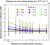 |
Fig. B.4 Accuracy of measured filament widths as a function of filament crest contrast. The dashed red line marks perfect accuracy. |
Figure B.5a and b displays our estimates of the measurement accuracy for the line mass parameter,  or
or  . At low filament contrast, the measurement error is again relatively large. As the contrast increases, both
  and
and  approach the true line masses. When the contrast exceeds 0.4, the average accuracy of
  estimates of the line mass is 0.14, −0.09, −0.17, −0.27, −0.32, −0.37, −0.39, −0.45 and −0.48, for model filaments with widths of 0.05, 0.08, 0.1, 0.13, 0.15, 0.18, 0.2, 0.3 and 0.4 pc respectively. For the same model filaments, the average accuracy of
  estimates is −0.04, −0.22, −0.29, −0.39, −0.43, −0.48, −0.51, −0.57 and −0.6, respectively. For filaments contrasts higher than 0.4, it thus appears that
  is a slightly better estimator of filament line mass than
  . However, when the contrast decreases from 0.4 to 0.1, the measurement accuracy of
  rapidly deterioriates, and
  becomes a slightly better estimator of line mass than
  . Above a contrast of 0.4, and considering all filament widths,
  typically underestimates the true Mline value by about 30 ± 20%, while
  leads to ~ 40 ± 20% underestimates.
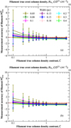 |
Fig. B.5 Accuracy of |


References
- Abe, D., Inoue, T., Inutsuka, S.-i., & Matsumoto, T. 2021, ApJ, 916, 83 [NASA ADS] [CrossRef] [Google Scholar]
- Allen, L., Bourke, T., Brooke, T., et al. 2006, Gould’s Belt: Star Formation in the Solar Neighborhood, Spitzer Proposal ID 30574 (USA: NASA) [Google Scholar]
- André, P. 2017, Comptes Rendus Geoscience, 349, 187 [Google Scholar]
- André, P., Men’shchikov, A., Bontemps, S., et al. 2010, A&A, 518, L102 [NASA ADS] [CrossRef] [EDP Sciences] [Google Scholar]
- André, P., Di Francesco, J., Ward-Thompson, D., et al. 2014, in Protostars and Planets VI, eds. H. Beuther, R. S. Klessen, C. P. Dullemond, & T. Henning (Tucson: University of Arizona), 27 [Google Scholar]
- André, P., Arzoumanian, D., Könyves, V., Shimajiri, Y., & Palmeirim, P. 2019, A&A, 629, L4 [Google Scholar]
- André, P. J., Palmeirim, P., & Arzoumanian, D. 2022, A&A, 667, L1 [CrossRef] [EDP Sciences] [Google Scholar]
- Arzoumanian, D., André, P., Didelon, P., et al. 2011, A&A, 529, L6 [NASA ADS] [CrossRef] [EDP Sciences] [Google Scholar]
- Arzoumanian, D., André, P., Peretto, N., & Könyves, V. 2013, A&A, 553, A119 [NASA ADS] [CrossRef] [EDP Sciences] [Google Scholar]
- Arzoumanian, D., André, P., Könyves, V., et al. 2019, A&A, 621, A42 [NASA ADS] [CrossRef] [EDP Sciences] [Google Scholar]
- Ballesteros-Paredes, J., André, P., Hennebelle, P., et al. 2020, Space Sci. Rev., 216, 76 [Google Scholar]
- Bally, J., Langer, W. D., Stark, A. A., & Wilson, R. W. 1987, ApJ, 312, L45 [NASA ADS] [CrossRef] [Google Scholar]
- Bernard, J. P., Paradis, D., Marshall, D. J., et al. 2010, A&A, 518, L88 [NASA ADS] [CrossRef] [EDP Sciences] [Google Scholar]
- Blitz, L. 1993, in Protostars and Planets III, eds. E. H. Levy, & J. I. Lunine (Tucson: University of Arizona Press), 125 [Google Scholar]
- Bohlin, R. C., Savage, B. D., & Drake, J. F. 1978, ApJ, 224, 132 [Google Scholar]
- Bracco, A., Bresnahan, D., Palmeirim, P., et al. 2020, A&A, 644, A5 [NASA ADS] [CrossRef] [EDP Sciences] [Google Scholar]
- Broekhoven-Fiene, H., Matthews, B. C., Harvey, P. M., et al. 2014, ApJ, 786, 37 [NASA ADS] [CrossRef] [Google Scholar]
- Chabrier, G. 2005, Astrophys. Space Sci. Lib., 327, 41 [NASA ADS] [CrossRef] [Google Scholar]
- Chung, E. J., Lee, C. W., Kim, S., et al. 2019, ApJ, 877, 114 [NASA ADS] [CrossRef] [Google Scholar]
- Di Francesco, J., Keown, J., Fallscheer, C., et al. 2020, ApJ, 904, 172 [NASA ADS] [CrossRef] [Google Scholar]
- Dunham, M. M., Crapsi, A., Evans, I., Neal J., et al. 2008, ApJS, 179, 249 [NASA ADS] [CrossRef] [Google Scholar]
- Ellsworth-Bowers, T. P., Glenn, J., Riley, A., et al. 2015, ApJ, 805, 157 [NASA ADS] [CrossRef] [Google Scholar]
- Federrath, C., & Klessen, R. S. 2013, ApJ, 763, 51 [Google Scholar]
- Fiege, J. D., & Pudritz, R. E. 2000, MNRAS, 311, 85 [Google Scholar]
- Finkbeiner, D. P. 2003, ApJS, 146, 407 [Google Scholar]
- Griffin, M. J., Abergel, A., Abreu, A., et al. 2010, A&A, 518, L3 [EDP Sciences] [Google Scholar]
- Guo, W., Chen, X., Feng, J., et al. 2021, ApJ, 921, 23 [NASA ADS] [CrossRef] [Google Scholar]
- Hacar, A., Clark, S. E., Heitsch, F., et al. 2023, ASP Conf. Ser., 534, 153 [NASA ADS] [Google Scholar]
- Hartmann, D., & Burton, W. B. 1997, Atlas of Galactic Neutral Hydrogen (Cambridge, UK: Cambridge University Press) [Google Scholar]
- Harvey, P. M., Fallscheer, C., Ginsburg, A., et al. 2013, ApJ, 764, 133 [NASA ADS] [CrossRef] [Google Scholar]
- Heigl, S., Gritschneder, M., & Burkert, A. 2018, MNRAS, 481, L1 [CrossRef] [Google Scholar]
- Henning, T., Linz, H., Krause, O., et al. 2010, A&A, 518, L95 [NASA ADS] [CrossRef] [EDP Sciences] [Google Scholar]
- Hill, T., Motte, F., Didelon, P., et al. 2011, A&A, 533, A94 [NASA ADS] [CrossRef] [EDP Sciences] [Google Scholar]
- Inoue, T., & Fukui, Y. 2013, ApJ, 774, L31 [Google Scholar]
- Inutsuka, S.-i. 2001, ApJ, 559, L149 [Google Scholar]
- Inutsuka, S.-i., & Miyama, S. M. 1997, ApJ, 480, 681 [NASA ADS] [CrossRef] [Google Scholar]
- Jeřábková, T., Hasani Zonoozi, A., Kroupa, P., et al. 2018, A&A, 620, A39 [Google Scholar]
- Juvela, M., Ristorcelli, I., Pagani, L., et al. 2012, A&A, 541, A12 [NASA ADS] [CrossRef] [EDP Sciences] [Google Scholar]
- Kirk, H., Myers, P. C., Bourke, T. L., et al. 2013, ApJ, 766, 115 [Google Scholar]
- Könyves, V., André, P., Men’shchikov, A., et al. 2015, A&A, 584, A91 [Google Scholar]
- Könyves, V., André, P., Arzoumanian, D., et al. 2020, A&A, 635, A34 [Google Scholar]
- Kramer, C., Stutzki, J., Rohrig, R., & Corneliussen, U. 1998, A&A, 329, 249 [NASA ADS] [Google Scholar]
- Kroupa, P., Weidner, C., Pflamm-Altenburg, J., et al. 2013, Planets, Stars and Stellar Systems, Galactic Structure and Stellar Populations, eds. T. D. Oswalt, & G. Gilmore, (Springer: Dordrecht), 5, 115 [NASA ADS] [CrossRef] [Google Scholar]
- Lada, E. A., Bally, J., & Stark, A. A. 1991, ApJ, 368, 432 [NASA ADS] [CrossRef] [Google Scholar]
- Lada, C. J., Lombardi, M., & Alves, J. F. 2009, ApJ, 703, 52 [NASA ADS] [CrossRef] [Google Scholar]
- Ladjelate, B., André, P., Könyves, V., et al. 2020, A&A, 638, A74 [NASA ADS] [CrossRef] [EDP Sciences] [Google Scholar]
- Lee, Y.-N., Hennebelle, P., & Chabrier, G. 2017, ApJ, 847, 114 [NASA ADS] [CrossRef] [Google Scholar]
- Li, D., & Goldsmith, P. F. 2012, ApJ, 756, 12 [NASA ADS] [CrossRef] [Google Scholar]
- Li, X.-M., Zhang, G.-Y., Men’shchikov, A. et al. 2023, A&A, 674, A225 [NASA ADS] [CrossRef] [EDP Sciences] [Google Scholar]
- Lim, T.-H., Min, K.-W., & Seon, K.-I. 2013, ApJ, 765, 107 [NASA ADS] [CrossRef] [Google Scholar]
- Marsh, K. A., Kirk, J. M., André, P., et al. 2016, MNRAS, 459, 342 [Google Scholar]
- Men’shchikov, A. 2013, A&A, 560, A63 [NASA ADS] [CrossRef] [EDP Sciences] [Google Scholar]
- Men’shchikov, A. 2017, A&A, 607, A64 [NASA ADS] [CrossRef] [EDP Sciences] [Google Scholar]
- Men’shchikov, A. 2021a, A&A, 654, A78 [NASA ADS] [CrossRef] [EDP Sciences] [Google Scholar]
- Men’shchikov, A. 2021b, A&A, 649, A89 [NASA ADS] [CrossRef] [EDP Sciences] [Google Scholar]
- Men’shchikov, A. 2023, A&A, 675, A185 [NASA ADS] [CrossRef] [EDP Sciences] [Google Scholar]
- Men’shchikov, A., André, P., Didelon, P., et al. 2010, A&A, 518, L103 [Google Scholar]
- Men’shchikov, A., André, P., Didelon, P., et al. 2012, A&A, 542, A81 [Google Scholar]
- Molinari, S., Swinyard, B., Bally, J., et al. 2010, A&A, 518, L100 [NASA ADS] [CrossRef] [EDP Sciences] [Google Scholar]
- Myers, P. C. 2009, ApJ, 700, 1609 [Google Scholar]
- Palmeirim, P., André, P., Kirk, J., et al. 2013, A&A, 550, A38 [NASA ADS] [CrossRef] [EDP Sciences] [Google Scholar]
- Pineda, J. E., Arzoumanian, D., André, P., et al. 2023, ASP Conf. Ser., 534, 233 [NASA ADS] [Google Scholar]
- Planck Collaboration XI. 2014, A&A, 571, A11 [NASA ADS] [CrossRef] [EDP Sciences] [Google Scholar]
- Poglitsch, A., Waelkens, C., Geis, N., et al. 2010, A&A, 518, L2 [NASA ADS] [CrossRef] [EDP Sciences] [Google Scholar]
- Rezaei Kh., S., & Kainulainen, J. 2022, ApJ, 930, L22 [NASA ADS] [CrossRef] [Google Scholar]
- Rice, T. S., Goodman, A. A., Bergin, E. A., Beaumont, C., & Dame, T. M. 2016, ApJ, 822, 52 [Google Scholar]
- Roy, A., André, P., Palmeirim, P., et al. 2014, A&A, 562, A138 [NASA ADS] [CrossRef] [EDP Sciences] [Google Scholar]
- Roy, A., André, P., Arzoumanian, D., et al. 2015, A&A, 584, A111 [NASA ADS] [CrossRef] [EDP Sciences] [Google Scholar]
- Salpeter, E. E. 1955, ApJ, 121, 161 [Google Scholar]
- Sancisi, R., Goss, W. M., Anderson, C., Johansson, L. E. B., & Winnberg, A. 1974, A&A, 35, 445 [NASA ADS] [Google Scholar]
- Schisano, E., Rygl, K. L. J., Molinari, S., et al. 2014, ApJ, 791, 27 [Google Scholar]
- Schlafly, E. F., Green, G., Finkbeiner, D. P., et al. 2014, ApJ, 786, 29 [NASA ADS] [CrossRef] [Google Scholar]
- Schneider, S., & Elmegreen, B. G. 1979, ApJS, 41, 87 [Google Scholar]
- Schneider, N., André, P., Könyves, V., et al. 2013, ApJ, 766, L17 [NASA ADS] [CrossRef] [Google Scholar]
- Shimajiri, Y., André, P., Ntormousi, E., et al. 2019a, A&A, 632, A83 [NASA ADS] [CrossRef] [EDP Sciences] [Google Scholar]
- Shimajiri, Y., André, P., Palmeirim, P., et al. 2019b, A&A, 623, A16 [NASA ADS] [CrossRef] [EDP Sciences] [Google Scholar]
- Shimajiri, Y., André, P., Peretto, N., et al. 2023, A&A, 672, A133 [NASA ADS] [CrossRef] [EDP Sciences] [Google Scholar]
- Solomon, P. M., Rivolo, A. R., Barrett, J., & Yahil, A. 1987, ApJ, 319, 730 [Google Scholar]
- Vâzquez-Semadeni, E., Kim, J., Shadmehri, M., & Ballesteros-Paredes, J. 2005, ApJ, 618, 344 [CrossRef] [Google Scholar]
- Vâzquez-Semadeni, E., Palau, A., Ballesteros-Paredes, J., Gomez, G. C., & Zamora-Avilés, M. 2019, MNRAS, 490, 3061 [CrossRef] [Google Scholar]
- Zhang, G.-Y., Xu, J.-L., Vasyunin, A. I., et al. 2018, A&A, 620, A163 [NASA ADS] [CrossRef] [EDP Sciences] [Google Scholar]
- Zhang, G.-Y., André, P., Men’shchikov, A., & Wang, K. 2020, A&A, 642, A76 [NASA ADS] [CrossRef] [EDP Sciences] [Google Scholar]
- Zucker, C., Speagle, J. S., Schlafly, E. F., et al. 2019, ApJ, 879, 125 [NASA ADS] [CrossRef] [Google Scholar]
The sensitivity of the Herschel/PACS observations of the California GMC was such that very-low-luminosity protostellar objects with 70 μm flux densities down to ~100mJy (Harvey et al. 2013) and accretion luminosities down <0.1 L⊙ (cf. Dunham et al. 2008) could be detected at the ~10σ level. Most (if not all) of the starless cores identified here, which lack significant emission in the PACS 70 μm data, are therefore truly starless.
This is analogous to constructing the integrated galaxy-wide IMF (IGIMF) by summing the IMFs of all star formation events in the whole galaxy at a given time (e.g., Jeřábková et al. 2018, and references therein).
Each filament segment is thus given a weight proportional to the total mass it harbors in the form of cores. The actual weights w(Mline) applied in Eq. (2) are normalized such as 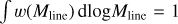 and are therefore dimensionless.
All Figures
|
Fig. 1 Location of the California GMC with respect to other nearby molecular cloud complexes. The three-color RGB map was created using publicly available data: 850 μm (red) and 350 μm (green) from Planck imaging, and 100 μm (blue) from IRAS (Planck Collaboration XI 2014, Public Data Release 2). The distances of the molecular clouds indicated on the map were inferred from Gaia DR2 parallaxes (Zucker et al. 2019). |
| In the text | |
|
Fig. 2 Column density map of the California GMC at an angular resolution of 18.2″, derived from Herschel data with hires (see Sect. 2). The positions of the dense cores identified with getsf (see Sect. 3.2) are overlaid and shown as ellipses of various colors according to core type (blue for robust prestellar cores, blue and brown for candidate prestellar cores, orange for unbound starless cores). For easier visibility, the full axes of the ellipses have twice the actual Gaussian full width at half maximum (FWHM) sizes. Protostellar cores are marked with black pentagrams. |
| In the text | |
|
Fig. 3 Column density probability distribution function (PDFN) obtained from the 18.2″ resolution image shown in Fig. 2, along with its structural components. For 2 ≤ Av ≤ 5, the PDFN follows a power law with an exponent of −3.2. It becomes slightly flatter for 5 ≤ Av ≤ 10, but its power-law exponent returns to −3.2 for Av > 10. |
| In the text | |
|
Fig. 4 Mass-size diagram for the cores identified in the California molecular cloud. “Extraction” represents the sizes measured directly on the 18.2″ column density map. “Decon. Robust”, “Decon. Candidate”, and “Decon. Unbound” represent the sizes of robust prestellar, candidate prestellar, and unbound starless cores, respectively, after deconvolution. The red solid line represents half of the mass of a thermally critical Bonnor-Ebert sphere (MBE/2) of radius R at a temperature of 10 K. The blue solid line marks the estimated threshold for selecting candidate prestellar cores. The dashed vertical line marks the 18.2″ beam size. |
| In the text | |
|
Fig. 5 Differential core mass function (ΔN/ΔlogM) for 927 starless cores (purple), 405 candidate prestellar cores and 209 robust prestellar cores. The vertical gray filled area at 0.45 ± 0.15 M⊙ denotes the estimated 90% completeness level for prestellar cores (see Appendix A). Error bars represent statistical uncertainties ( |
| In the text | |
|
Fig. 6 Median candidate prestellar core mass plotted against background cloud column density (AV units) is shown by the black triangles. The error bars represent the inter-quartile range of observed masses within each bin. The green dashed line depicts a linear fit to the median masses as a function of AV,bg, given by Mmed ∝ (0.2 ± 0.02) × AV,bg. The blue dash-dotted line corresponds to a linear fit to the upper quartiles of median observed masses, while the magenta dotted line represents a linear fit to the lower quartiles. |
| In the text | |
|
Fig. 7 Global filament network including all transverse angular scales up to ±80″ across the filament spines. A thick skeleton mask with a fixed line width of about 4 pixels (12″), color-coded as shown in the bar on the right, is overlaid on the original column density image shown as a grayscale background. Map values at the skeleton pixels correspond to background- and source-subtracted column densities on the filament crests. |
| In the text | |
|
Fig. 8 Close-up view of the filament network (left) and example of a filament radial profile (right). Left: skeletons of several filaments depicted as grey solid curves and traced within a 20′ × 20′ subfield of the column density image at 18.2″ resolution. The black curve represents the skeleton of the filament whose radial profile is displayed in the right panel. Right: median one-sided column density profiles measured on both the left (purple solid line) and right (blue) sides of the filament, with the black dashed curve representing the beam profile. The median half maximum width measured on the left (north-east) side is 0.13 pc, that on the right (south-west) side is 0.17 pc, and the mean is 0.15 pc. |
| In the text | |
|
Fig. 9 Distributions of widths, dust temperatures, and radial density gradients for filament skeletons and chunks (with C > 0.2 and C > 0.4). (a) Distribution of measured FWHM widths. (b) Distribution of median dust temperatures measured on filament crests. (c) Histogram of logarithmic slopes s for the column density profiles of all measured filaments. (If both sides of a filament were effectively measured, the histogram count was incremented by 2; if only one side was measured, the histogram count was incremented by 1; if neither side could be measured, the histogram count was not incremented.) The median and peak values of each parameter are provided in the legend of the corresponding panel. |
| In the text | |
|
Fig. 10 Correlations between filament properties, (a) Filament crest column density against column density contrast. The blue solid line is the fit: |
| In the text | |
|
Fig. 11 Spatial relationship between extracted cores and supercritical filamentary structures, displayed as an histogram of separations between core centers and the nearest supercritical filamentary structures. |
| In the text | |
|
Fig. 12 Filament line mass function (FLMF, ΔN/ΔlogMline), derived from the sample of filament chunks in the California GMC. The error bars represent statistical uncertainties ( |
| In the text | |
|
Fig. 13 Differential core formation efficiency (CFE) in the California GMC as a function of background cloud column density (blue histogram with error bars) and parent filament column density (magenta histogram), both expressed in AV units. The CFE values were obtained by dividing the mass in the form of candidate prestellar cores in a given column density bin by the cloud mass (blue histogram) or estimated filament mass (magenta histogram) in the same column density bin. The upper x-axis provides a rough estimate of the equivalent filament line mass assuming the parent filament of each core has an effective width 0.18 pc (corresponding to the median observed filament width – see Sect. 3.3.1). The vertical dashed line marks the position of the thermally critical line mass Mline,crit ~ 16 M⊙pc−1, corresponding to AV,bg ~ 4.5. The red and green curves show simple fits to the blue and magenta histograms, respectively, with a smooth step function of the form CFE(AV) = CFEmax[1 − exp(a × AV + b)], with CFEmax ≈ 30%. For the blue distribution, α = −0.16 and b = 0.4; for the magenta distribution, α = −0.28 and b = 0.25. |
| In the text | |
|
Fig. 14 Comparison of the prestellar CMFs (in ΔN/ΔlogM format) expected in the toy model described in André et al. (2019) and in the text (solid and dashed curves) with the observed prestellar CMFs observed in the California GMC (data points and histograms) at low column densities ( |
| In the text | |
|
Fig. A.1 Mass–size diagram of the cores detected in the simulated Herschel images. The red line represents half of the critical Bonnor-Ebert mass (MBE/2) at 10 K as a function of radius. The blue line shows the empirical threshold used to select candidate prestellar cores in Sect. 3.2 (cf. Fig. 4), which captures 95% of the synthetic prestellar cores in the simulation. The curves labeled RBES (in magenta) show the mass vs. radius relations for the convolved model cores, while the lines labeled RAS (in green) represent the true mass vs. radius relations of the models. The black dashed vertical line shows the minimum derived model size (MMS) used when applying simple Gaussian deconvolution to the simulated extraction results (see Sect. 3.2). |
| In the text | |
|
Fig. A.2 Accuracy of core measurements according to the simulations, a) Measured FWHM radius versus model radius (RBES)- Perfect core radius estimates would lie on the horizontal magenta dotted line. The horizontal solid line marks the median ratio value for cores with M > 0.25 M⊙. b) SED-derived temperature against true dust temperature of the model, c) SED-derived and |
| In the text | |
|
Fig. A.3 Tests for estimating the completeness of core extractions based on the simulations, a) Fraction of recovered synthetic cores as a function of true core mass. The error bars represent the ±1σ deviation within each mass bin and the magenta dotted line marks 100% completeness, b) Recovered CMF after extracting the simulated cores and binning the results according to true core mass, c) Recovered CMF after extracting the simulated cores and binning the results according to SED-derived mass. |
| In the text | |
|
Fig. B.1 Simulated 3.3° × 1.1° column density image of a filamentary cloud at 18.2″ resolution: (a) large-scale background produced by the getsf analysis of the California data; (b) synthetic background cloud; (c) skeletons detected by getsf in the X-shaped nebula; (d) simulated filaments; (e) complete synthetic image of the simulated filamentary cloud. |
| In the text | |
|
Fig. B.2 Illustrative example of an artificially straightened filament with a width of W = 0.1 pc, a contrast of C = 1, and a power-law exponent of s = −1.5. |
| In the text | |
|
Fig. B.3 Fraction of recovered model filaments with various intrinsic widths (solid lines) as a function of column density contrast. The red dashed horizontal line marks an 80% completeness level. The dotted lines represent the fraction of spurious filaments. |
| In the text | |
|
Fig. B.4 Accuracy of measured filament widths as a function of filament crest contrast. The dashed red line marks perfect accuracy. |
| In the text | |
|
Fig. B.5 Accuracy of |
| In the text | |
Current usage metrics show cumulative count of Article Views (full-text article views including HTML views, PDF and ePub downloads, according to the available data) and Abstracts Views on Vision4Press platform.
Data correspond to usage on the plateform after 2015. The current usage metrics is available 48-96 hours after online publication and is updated daily on week days.
Initial download of the metrics may take a while.