| Issue |
A&A
Volume 629, September 2019
|
|
|---|---|---|
| Article Number | A81 | |
| Number of page(s) | 44 | |
| Section | Interstellar and circumstellar matter | |
| DOI | https://doi.org/10.1051/0004-6361/201935260 | |
| Published online | 12 September 2019 | |
Dynamics of cluster-forming hub-filament systems
The case of the high-mass star-forming complex Monoceros R2
1
Department of Space, Earth and Environment, Chalmers University of Technology,
412 93 Gothenburg, Sweden
e-mail: This email address is being protected from spambots. You need JavaScript enabled to view it.
2
Observatorio Astronómico Nacional, Apdo. 112,
28803
Alcalá de Henares Madrid, Spain
3
I. Physikalisches Institut, Universität zu Köln,
Zülpicher Str. 77, 50937 Köln, Germany
4
Laboratoire AIM, Paris-Saclay, CEA/IRFU/SAp – CNRS – Université Paris Diderot,
91191 Gif-sur-Yvette Cedex, France
5
Max-Planck-Institute for Astronomy,
Königstuhl 17, 69117 Heidelberg, Germany
6
Instituto de Radioastronomía y Astrofísica, Universidad Nacional Autónoma de México,
PO Box 3-72, 58090 Morelia, Mexico
7
Institut de Physique du Globe de Paris, Sorbonne Paris Cité, Université Paris Diderot, UMR 7154 CNRS, 75005 Paris, France
8
IRAP, Université de Toulouse, CNRS, UPS, CNES,
9 Av. colonel Roche, BP 44346, 31028 Toulouse Cedex 4, France
9
Instituto de Astrofísica de Andalucía, IAA-CSIC, Glorieta de la Astronomía s/n,
18008 Granada, Spain
10
Institut de Radioastronomie Millimétrique (IRAM),
300 rue de la Piscine, 38406 Saint Martin d’Hères, France
11
Instituto Nacional de Astrofísica, Óptica y Electrónica, Luis Enrique Erro #1,
72840 Tonantzintla, Puebla, Mexico
12
Instituto de Física Fundamental (CSIC). Calle Serrano 121,
28006, Madrid, Spain
13
Zentrum für Astronomie, Institut für Theoretische Astrophysik, Universität Heidelberg,
Albert-Ueberle-Str. 2, 69120 Heidelberg, Germany
Received:
12
February
2019
Accepted:
5
July
2019
Abstract
Context. High-mass stars and star clusters commonly form within hub-filament systems. Monoceros R2 (hereafter Mon R2), at a distance of 830 pc, harbors one of the closest of these systems, making it an excellent target for case studies.
Aims. We investigate the morphology, stability and dynamical properties of the Mon R2 hub-filament system.
Methods. We employed observations of the 13CO and C18O 1 →0 and 2 →1 lines obtained with the IRAM-30 m telescope. We also used H2 column density maps derived from Herschel dust emission observations.
Results. We identified the filamentary network in Mon R2 with the DisPerSE algorithm and characterized the individual filaments as either main (converging into the hub) or secondary (converging to a main filament). The main filaments have line masses of 30–100 M⊙ pc−1 and show signs of fragmentation, while the secondary filaments have line masses of 12–60 M⊙ pc−1 and show fragmentation only sporadically. In the context of Ostriker’s hydrostatic filament model, the main filaments are thermally supercritical. If non-thermal motions are included, most of them are transcritical. Most of the secondary filaments are roughly transcritical regardless of whether non-thermal motions are included or not. From the morphology and kinematics of the main filaments, we estimate a mass accretion rate of 10−4–10−3 M⊙ yr−1 into the central hub. The secondary filaments accrete into the main filaments at a rate of 0.1–0.4 × 10⁻⁴ M⊙ yr−1. The main filaments extend into the central hub. Their velocity gradients increase toward the hub, suggesting acceleration of the gas. We estimate that with the observed infall velocity, the mass-doubling time of the hub is ~2.5 Myr, ten times longer than the free-fall time, suggesting a dynamically old region. These timescales are comparable with the chemical age of the HII region. Inside the hub, the main filaments show a ring- or a spiral-like morphology that exhibits rotation and infall motions. One possible explanation for the morphology is that gas is falling into the central cluster following a spiral-like pattern.
Key words: ISM: kinematics and dynamics / ISM: structure / ISM: clouds / ISM: individual objects: Monoceros R2
© ESO 2019
1 Introduction
In recent decades, our view of star-forming regions has been undergoing a revolution thanks to the new observational facilities. Space telescopes such as Spitzer and Herschel provided observations of a large number of molecular clouds that have revealed a ubiquity of filamentary structures containing stars in different evolutionary stages (e.g., Schneider & Elmegreen 1979; Loren 1989a,b; Nagai et al. 1998; Myers 2009; André et al. 2010; Molinari et al. 2010; Schneider et al. 2010; Busquet et al. 2013; Stutz et al. 2013; Kirk et al. 2013; Peretto et al. 2014; Fehér et al. 2016; Abreu-Vicente et al. 2016). Filamentary structures pervading clouds are unstable against both radial collapse and fragmentation (e.g., Larson 1985; Miyama et al. 1987a,b; Inutsuka & Miyama 1997), and although their origin or formation process is still unclear, turbulence and gravity (e.g., Klessen et al. 2000; André et al. 2010) can produce, together with the presence of magnetic fields (e.g., Molina et al. 2012; Kirk et al. 2015), the observed structures. It is thought that star formation occurs preferentially along the filaments, with high-mass stars forming in the highest density regions where several filaments converge, called ridges or hubs (NH ~ 1023 cm−2 and  cm−3, e.g., Schneider et al. 2010, 2012; Liu et al. 2012; Peretto et al. 2013, 2014; Louvet et al. 2014). This suggests that filaments precede the onset of star formation, funneling interstellar gas and dust into increasingly denser concentrations that will contract and fragment, leading to gravitationally bound prestellar cores that will eventually form both low- and high-mass stars. Following this process,high-mass stars can inject large amounts of radiation and turbulence in the surrounding medium that may affect the structural properties of filaments, leading to a different level of fragmentation (e.g., Csengeri et al. 2011; Seifried & Walch 2015, 2016).
In the recent years, an increasing number of works have focused on the study of the dynamics and fragmentation of filamentary structures from both the observational and theoretical points of view (see e.g., André et al. 2010; Schneider et al. 2010, 2012; Hennemann et al. 2012; Busquet et al. 2013; Galvan-Madrid et al. 2013; Hacar et al. 2013, 2018; Peretto et al. 2013; Louvet et al. 2014; Tafalla & Hacar 2015; Smith et al. 2014; Henshaw et al. 2014; Tackenbergt et al. 2014; Seifried & Walch 2016; Kainulainen et al. 2017; Seifried et al. 2017; Arzoumanian et al. 2019; Williams et al. 2018; Clarke et al. 2019). However, few of these works focus on massive star-forming regions within hub-filament system, and little is known about the dynamics of filamentary networks (e.g., cluster-forming hub filament systems) and their role in the accretion processes that regulate the formation of high-mass star-forming clusters. In addition, most of the research on high-mass star-formingregions focuses on the study of one particular cloud: the Orion A molecular cloud (e.g., Hacar et al. 2018; Suri et al. 2019). Thus, and with the goal of having a better understanding of the filament properties in high-mass star-forming regions, it isnecessary to study other massive clouds. For this, the Monoceros star-forming complex appears to be an ideal target.
Located at a distance of only 830 pc (Herbst & Racine 1976), Monoceros R2 (hereafter Mon R2) is an active massive star-forming cloud that hosts one of the closest ultracompact (UC) HII regions. Recently, Herschel observations have revealed an intriguing look of the cloud with several filaments converging into the central area (~ 2.25 pc2, see left panel in Fig. 1; Didelon et al. 2015; Pokhrel et al. 2016; Rayner et al. 2017). A number of hot bubbles and already developed HII regions are identified throughout the region (visible in blue in the image shown in Fig. 1, left) mainly in the outskirts of the central and densest region, where a cluster of young high-mass stars is found to be forming at the junction (or hub) of the filamentary structures. The most massive star of this infrared cluster is IRS 1, at α(J2000) = 06h07m46.2s, δ(J2000) = − 06°23′08.3″, with a mass of ~ 12 M⊙ (e.g., Thronson et al. 1980; Giannakopoulou et al. 1996). This source is driving an UC HII region that has created a cavity free of molecular gas extending for about 30′′ (or 0.12 pc, e.g., Choi et al. 2000; Dierickx et al. 2015) and surrounded by a number of photon-dominated regions (PDRs) with different physical and chemical conditions (e.g., Ginard et al. 2012; Pilleri et al. 2012; Treviño-Morales et al. 2014, 2016). Based on Herschel PACS and SPIRE maps, Didelon et al. (2015) determined that the central region hosting the UC HII region shows a power-law density profile of ρ(r) ∝ r−2.5. This density profile was attributed to an external pressure certainly associated with global collapse. Rayner et al. (2017) studied the distribution of dense cores and young stellar objects in the region and proposed that the hub may be sustaining its star formation by accretion of material from the large-scale mass reservoir (see also Treviño-Morales 2016).
In summary, thanks to its morphology, proximity and general characteristics, Mon R2 appears to be one of the clearest examples of a hub-filament system, thus being an excellent target to study in detail the physical properties of these systems. In this paper, we report observations of the Mon R2 star-forming region conducted with the IRAM-30 m telescope. We observed different molecular line transitions that allow us to study the molecular gas content in the region, and for the first time, study the large-scale gas dynamics of its filamentary structure. The observational data are introduced in Sect. 2. In Sect. 3, we present the large-scale structure of the molecular gas (at parsec scales), while in Sect. 4 we analyze the filamentary structure in Mon R2, giving special emphasis on the kinematic properties and zooming into the central hub. A general discussion and a summary of the main results are presented in Sects. 5 and 6, respectively.
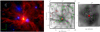 |
Fig. 1 Left: three-color image of the Mon R2 cluster-forming hub-filaments system. Red: H2 column density map derived from Herschel SPIRE and PACS observations (Didelon et al. 2015), green: 1.65 μm band of the Two Micron All Sky Survey (Skrutskie et al. 2006), and blue: 560 nm band of the Digitalized Sky Survey (Lasker et al. 1990). Center: Herschel H2 column density (in cm−2, Didelon et al. 2015). The black polygon shows the area surveyed with the IRAM-30 m telescope, while the white box corresponds to the inner 0.7 pc × 0.7 pc around the central hub and zoomed in the right panel. Right: Herschel H2 column density (in cm−2) of the central hub of Mon R2. Gray contours show the H13CO+ (3 →2) emission tracing the high-density molecular gas (Treviño-Morales et al. 2014). The red star gives the position of IRS 1 (with coordinates α(J2000) = 06h 07m 46.2s, δ(J2000) = − 06°23′08.3″). White stars indicate the positions of infrared sources. The white circle indicates the beam size of the IRAM-30 m telescope at 100 GHz(see Sect. 2). The colored symbols are the sources identified by Rayner et al. (2017): pink stars are protostars, green circles are bound clumps, and red triangles are unbound clumps. |
Observational parameters of the main detected lines.
2 Observations and data reduction
We observed the Mon R2 star-forming region with the IRAM-30 m telescope (Pico Veleta, Spain). The observations were conducted between July 2014 and December 20161 under good weather conditions, with precipitable water vapor (pwv) between 1 and 3 mm and τ ~ 0.06–0.182. We used the on-the-fly (OTF) mapping technique to cover a field of view of 855 arcmin2 at 3 mm indual polarization mode using the EMIR receivers (Carter et al. 2012), with the fast Fourier transform spectrometer (FTS) at 50 kHz of resolution (Klein et al. 2012). The observed area is indicated with a black polygon in the middle panel of Fig. 1, where the offset [0′′,0′′] corresponds to the position of the IRS 1 star. The molecular spectral lines covered and detected within our spectral setup are listed in Table 1. During the observations, the pointing was corrected by observing the strong nearby quasar 0605−058 every 1–2 h, and the focus by observing a planet every 3–4 h. Pointing and focus corrections were stable throughout all the runs.
The data were reduced with a standard procedure using the CLASS/GILDAS package3 (Pety et al. 2005). For each molecular transition listed in Table 1, we created individual data cubes centered at the source velocity (vLSR = 10 km s−1), and spanning a velocity range of ± 60 km s−1. The native spectral resolution across the whole observed frequency band varies between 0.13 and 0.16 km s−1. In order to perform a proper comparison of the line profiles of every molecule, we smoothed it to a common value of 0.17 km s−1. A two-order polynomial baseline was applied for baseline subtraction. The final data do not show platforming effects and/or spikes (bad channels) in the observed sub-bands. The emission from the sky was subtracted using different reference positions, which were observed every 2 min for a duration of 20 s. Single-pointing observations of the reference positions revealed the presence of weak 13CO (1 →0) emission (TMB < 300 mK), but not from the other transitions included in the setup. We corrected the 13CO (1 →0) emission data cube of Mon R2 by adding synthetic spectra derived from Gaussian fits to the emission found in the reference positions. Throughout this paper, we use the main beam brightness temperature (TMB) as intensity scale, while the output of the telescope is usually calibrated in antenna temperature ( ). The conversion between
  and TMB is done by applying the factor Feff∕Beff, where Feff is the forward efficiency which equals 95%, and Beff is the beam efficiency (see Table 1).
In addition to the IRAM-30 m data at 3 mm, we also make use of complementary C18O and 13CO (2 →1) maps. These maps were obtained with the IRAM-30 m telescope during 2013 (PI: P. Pilleri). The observations were performed using the same technique described above, but combining the EMIR receivers with the FTS backed at 200 kHz of resolution. The J = 2 →1 maps cover an area of about 10 arcmin2 around the IRS 1 star. The data were processed following the strategy described above.
3 Parsec-scale molecular emission
Figure 2 shows the spectra for the detected species averaged over an area of 3′ ×3′ (or 0.7 pc × 0.7 pc at the distance of Mon R2), corresponding to the inner part of the hub (see Fig. 1, right). Among all the detected species, 13CO, C18O, HNC, and N2 H+ are the brightest with TMB ≥ 1 K. For these species, the emission spans a velocity range of ~ 13 km s−1 for 13CO, ~ 8–10 km s−1 for C18O and HNC, and ~ 5 km s−1 for N2 H+. The emission from the other species (i.e., HC3N, SO, CCS, and NH2D) spans a velocity range of 4–6 km s−1 and presents weaker intensities with TMB < 1 K. In Fig. 3, we show the maps of integrated intensity (left column), velocity centroid (middle column), and linewidth (right column) for the 13CO (1 →0), C18O (1 →0), HNC (1 →0), and N2 H+ (1 →0) molecular lines (rows, from top to bottom). The velocity range considered includes emission above 3σ (see red dashed vertical lines in Fig. 2).
As seen in the top panels of Fig. 3, the CO isotopologs show extended emission distributed across all the surveyed area revealing a set of filaments coming from all directions to flow into the central hub. For clarity, we refer to the various relevant structures seen in the maps as N for the north-south elongated structure, NE for the structure to the northeast of the central hub, E for the structure extending to the east, and SW for the emission toward the southwest of the central area. For the HNC and N2 H+ species (see bottom panels), the emission is mainly found in the central region. However, these species also show faint extended emission coincident with the elongated structures identified in the 13CO and C18O maps. The lack of N2 H+ emission within the elongated structures might mean that CO could be frozen out outside the central hub. These structures are also traced by HNC and N2 H+, but their lower abundances result in a lower signal to noise ratio (S/N) which challenges their detection. In the following, we use the 13CO and C18O (1 →0) lines to study the physical properties and kinematics of the extended structures in Mon R2.
The central area around IRS 1 is bright in all the observed species, but some different features can be distinguished. The emission of most of the detected species appears mainly in an arc-shell structure surrounding the central cluster of infrared stars (see red star in Fig. 3 and right panel of Fig. 1) that pinpoint the location of newly formed stars in Mon R2. The arc structure points toward the south of the infrared cluster, in agreement with the cometary shape of the HII region as revealed in previous works (e.g., Ginard et al. 2012; Pilleri et al. 2012; Martí et al. 2013). The observed species present their strongest emission to the northeast and southwest of the infrared cluster. The HNC and N2 H+ maps show a third bright peak to the south of the cluster, where the CO intensity decreases. This spatial differentiation may be due to different physical conditions causing 13CO and C18O to be depleted onto dust grains and/or a high opacity that results in self-absorption of the CO lines. However, the spectra at these positions show Gaussian profiles with no signatures of self-absorption. A more detailed study of the chemical properties in this region is thesubject of a forthcoming paper.
The middle column of panels in Fig. 3 show the velocity field as determined from the first-order moment analysis. The region presents complex kinematics with different velocity components and velocity gradients. On large scales, there is a global velocity gradient (~ 1.5 km s−1 pc−1) from east to west. On smaller scales, we do not find a clear velocity gradient along the N structure, with most of the emission at systemic velocities (~ 10 km s−1). The NE structure is mainly blue-shifted, with a velocity ~ 8.5 km s−1. The E structure shows a velocity gradient of ~ 3 km s−1 from east (at 7.5 km s−1) to the center of the region (at 10.5 km s−1). Finally, the southern part of SW is red-shifted (11 km s−1), but shows a velocity gradient toward the central part, reaching a velocity of 9.5 km s−1. In addition to the longitudinal gradients, these four structures also show signatures of smaller velocity gradients (~ 1 km s−1) across them. The velocity features of these structures are studied in more detail in Sect. 4.4. The velocity structure around the hub is similar in all the species with a prominent northeast-southwestern velocity gradient. Interestingly, the blue-shifted gas is reminiscent of an elongated curved structure that starts to the west of IRS 1 and approaches the center through the north. The red-shifted emission, although not as clear as for the blue-shifted component, also seems to converge toward the IRS 1 position from the east and then south, constituting a complementary curved structure to the blue-shifted emission (see Sect. 4.5 for a detailed discussion).
The right column of panels of Fig. 3 show the velocity dispersion as determined from the second-order moment analysis. The extended emission has a constant, relatively narrow linewidth of ~ 1–1.5 km s−1, which increases toward the central part, reaching a maximum value of ~ 6 km s−1 for 13CO, ~ 4 km s−1 for C18O, ~ 4 km s−1 for HNC, and ~ 2.0 km s−1 for N2 H+. These large linewidths are more likely the consequence of the complex kinematics in the inner region, which is not resolved by the IRAM-30m beam.
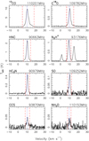 |
Fig. 2 Spectra averaged over an area of 0.7 pc × 0.7 pc centered at the position of IRS 1 (corresponding to the area shown in Fig. 1, right). The blue dotted vertical line indicates the source velocity (vLSR = 10 km s−1). The red dashed vertical lines indicate the velocity range where the S∕N is above 3σ for the molecular emission. These ranges are used to generate the integrated intensity maps presented in Fig. 3. The velocity ranges correspond to 5–18 km s−1 for 13CO, 7–15 km s−1 for C18O, 6–14 km s−1 for HNC, and 7–12 km s−1 for N2 H+. |
4 Filamentary network of Mon R2
In the following section we analyze the structure of the dense gas in Mon R2, concentrating on the characterization of the filamentary structure previously seen in dust continuum emission maps with Herschel and now, for the first time, resolved in velocity in different molecular species. In Sects. 4.1 and 4.2 we derive column density maps from molecular line emission and identify filamentary structures from the position-position-velocity data cubes. The stability of the filaments is explored in Sect. 4.3, and their kinematic properties are discussed in Sect. 4.4. We study the convergence of the filaments into the central hub in Sect. 4.5.
4.1 Column density structure
The integrated intensity maps of the 13CO and C18O (1 →0) lines reveal the existence of several filamentary structures converging into the central hub (see Fig. 3). These filamentary structures are also detected in the H2 column density map derived from the Herschel continuum emission maps (see Didelon et al. 2015). Complementary to the H2 column density maps, we derive column density maps for the 13CO and C18O species. Assuming local thermodynamic equilibrium (LTE) and optically thin molecular emission, the column densities are calculated (see Appendix A) as
![Mathematical equation: \begin{equation*}\left[\frac{N(^{13}\mathrm{CO})}{\mathrm{cm}^{-2}}\right] = 4.69\times10^{13} T_{\mathrm{ex}} \textrm{e}^{\frac{5.30}{T_{\mathrm{ex}}}} \left[\frac{\int T(v)~\textrm{d}v}{\mathrm{K~km~s}^{-1}}\right], \end{equation*}](/articles/aa/full_html/2019/09/aa35260-19/aa35260-19-eq4.png) (1)
(1)
and
![Mathematical equation: \begin{equation*}\left[\frac{N(\mathrm{C}^{18}\mathrm{O})}{\mathrm{cm}^{-2}}\right] = 4.73\times10^{13} T_{\mathrm{ex}} \textrm{e}^{\frac{5.28}{T_{\mathrm{ex}}}} \left[\frac{\int T(v)~\textrm{d}v}{\mathrm{K~km~s}^{-1}}\right], \end{equation*}](/articles/aa/full_html/2019/09/aa35260-19/aa35260-19-eq5.png) (2)
(2)
where Tex is the excitation temperature in K, and the term ∫ T(v) dv is the integrated flux of the (1 →0) line in K km s−1. We assume that the lines are thermalized with the excitation temperature being equal to the gas kinetic temperature (i.e., Tex = Tk) and that this equals the dust temperature, Tdust, as derived in Didelon et al. (2015, see top-right panel in Fig. 4). This assumption is only accurate in dense regions (n > 104 cm−3) shielded from the UV radiation. Hence, in the surroundings of the central UC HII region and the PDRs, the UV radiation will increase the gas temperature(Tgas), and Tgas = Tdust should be considered as a lower limit to the real temperature. We smoothed the IRAM-30 m molecular maps to the angular resolution of the Herschel-derived Tdust map (i.e., 36′′) and used Eqs. (1) and (2) to derive the molecular column density maps shown in Fig. 4. The highest column densities are found toward the central hub with N(13CO) > 5 × 1016 cm−2. Outside the hub, we find a constant column density of N(13CO) ≈ 1 × 1016 cm−2 with local enhancements associated with the filamentary structures. For C18O, we derive column densities ≃10 times lower than for 13CO.
We nextpresent our study of the internal structure of the cluster-forming region; our specific aim was to determine whether a well-defined hub can be identified, and if so, to measure its size and average radial parameters. To this end, we studied the azimuthally averaged mass and surface density of the cloud within concentric circles and rings centered at IRS 1. The radius of the circles, Rcir, ranges from 0.1 pc to 2.4 pc (or 25′′– 600′′, the radius of the UC HII region is 12.5′′), while the ring radius Rring is the difference of an external circle Rcir,out and an innercircle Rcir,in. In Fig. 5, we plot the azimuthally averaged radial profiles for 13CO (top panels) and C18O (bottom panels). We first considered the radially integrated gas mass Mcir (first column of panels) calculated in circles of radius Rcir, and then, we calculated the gas massMring (third column of panels) over concentric rings with radius Rring = Rcir,out − Rcir,in. The gas mass M within each circle or ring is given by
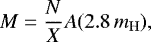 (3)
(3)
where N is the total column density of the molecule (as derived in Eqs. (1) and (2), X is the relative abundance of the molecule with respect to H2, A is the surface area of the circle, and mH is the hydrogen atom mass. We used the typical Mon R2 abundances X(13CO) = 1.7 × 10⁻⁶ and X(C18O) = 1.7 × 10⁻⁷ (e.g., Ginard et al. 2012). These values are consistent with the average abundances that can be derived by comparing the H2 (from Herschel) and the 13CO and C18O column density maps (see Fig. B.1). Figure 5 also shows the radially integrated gas mass divided by the surface area of the circles (second column of panels) and the concentric ring’s mass divided by the ring’s surface area (fourth column of panels), i.e., the surface densities profiles. The radial profiles of the surface density in Fig. 5 show two different slopes (yellow dotted lines) with the turnover point occurring at a radius between 200′′ and 300′′ (or 0.8–1.2 pc). This change in slope may result from a transition between a denser region in the center and a more diffuse component on the outside. We therefore consider that there is a well-defined hub structure with a radius of about 250′′, or 1 pc. Hereafter, we refer to this as the hub radius, Rhub. We note that the radial mass and surface density profiles do not correspond to the initial mass distribution of the cloud. They are just a tool to investigate the morphology of the current evolutionary stage of the cloud.
From the 13CO and C18O column density maps, we estimated a mass of ~ 1700 M⊙ within the Rhub = 1 pc, which corresponds to about 24% of the total mass (~ 7200 M⊙) of the surveyed area. From the H2 column density maps obtained with Herschel observations (Didelon et al. 2015), we derived the mass of ~ 3600 M⊙ for the hub and ~ 8300 M⊙ for the surveyed area. These are in reasonable agreement with the values derived from the molecular species (see Table 2). In summary, considering the different tracers, we find that about 32% of the mass in the surveyed area is contained in the central hub.
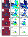 |
Fig. 3 Left column panels: integrated intensity maps over the whole surveyed area for the (1 →0) transition lines of the 13CO, C18O, HNC and N2H+ molecules. Middle column: velocity centroid. Right column panels: linewidth. The maps were produced by computing the zero-order (left), first-order (middle) and second-order (right) moments in the velocity range defined in Fig. 2. The yellow labels and the dotted lines indicate the main features identified in the region. The red star at (0′′,0′′) offset gives the position of IRS 1. |
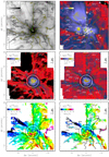 |
Fig. 4 Top panels: H2 column density (left) and dust temperature (right) maps from Herschel (Didelon et al. 2015). Middle panels: 13CO (left) and C18O (right) column density maps. Bottom panels: velocity centroid for 13CO (left) and C18O (right). The “skeleton” of identified filaments are marked with solid white, black, or yellow lines. The black and white circles correspond to the radii at 200′′, 250′′, and 300′′ (transition between thehub and the filaments, see Fig. 5). The white circles in the top right panel shows sources identified bySokol et al. (2019); the colored symbols show the sources identified by Rayner et al. (2017). |
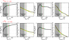 |
Fig. 5 Azimuthally averaged mass and surface density derived from the 13CO (top) and C18O (bottom) column density maps. From left to right: each column shows (i) radially integratedmass, (ii) radially integrated mass divided by the area of the circle with radius Rcir (i.e., radially integrated surface density), (iii) concentric annular mass, (iv) concentric annular surface density. The radially integrated mass and surface density were calculated within circles of radius Rcir centered on IRS 1 from R = 25″ (~ 0.1 pc) to R = 600″ (~ 2.4 pc). The concentric annular mass and surface density were calculated within concentric rings of radius Rring =Rcir,out − Rcir,in = 36″ (corresponding to the Herschel beam size). In order to do a direct comparison of the profiles, the x-axis in the concentric annular mass and surface density profiles correspond to Rcir,out. The yellow dotted lines indicate the different slopes in the surface density profiles. The light gray zone indicates the transition between the hub and the filaments, from 200′′ to 300′′. The dark gray area marks the central hub with Rhub = 250” = 1 pc. |
4.2 Filament identification
As shown in Fig. 4, Mon R2 has a filamentary structure outside the central hub. Making use of our 3D data cubes (position–position–velocity) we used the structure identification algorithm Discrete Persistent Structures Extractor (DisPerSE, Sousbie 2011) to define filaments. DisPerSE was originally developed to search for filamentary structures in large-scale cosmological simulations, but it has been successfully applied to identify filaments from molecular clouds and from numerical simulations of star-forming regions (e.g., Arzoumanian et al. 2011; Schneider et al. 2012; Palmeirim et al. 2013; Smith et al. 2014; Panopoulou et al. 2017; Zamora-Avilés et al. 2017; Chira et al. 2018; Suri et al. 2019). DisPerSE identifies critical points in a data set where the gradient of the intensity goes to zero and connects them with arcs; the arcs are then called filaments. The critical point pairs that form an arc with low significance can be eliminated with two thresholds: the persistence threshold and the detection threshold. The persistence is expressed as the difference between the intensities of critical points in a pair. The higher the persistence, the more contrast the structure has. The detection threshold eliminates the critical points that are below the noise. We used the 13CO emission map for filament identification with DisPerSE, and set both the persistence and the detection thresholds to be five times the noise level per channel. These thresholds assure that we select filaments with high significance.
Complementing the identification of filaments with DisPerSE, we visually inspected the correspondence between the DisPerSE-identified filaments and elongated structures visible in the 13CO (1 →0) and C18O (1 →0) data sets. Most of the structures identified with DisPerSE are clearly visible in at least one velocity interval and appear contiguous in successive velocity channels, which further supports the picture that they are coherent entities in the position-position-velocity space. Only few structures are not clearly identified in the molecular channel maps and have been discarded. Thus, our final set of filaments consists of those DisPerSE identified structures that are confirmed via visual inspection in both 13CO and C18O emission through different velocity intervals.
The skeletons of the identified filaments are shown in Fig. 4. A comparison of the filaments with the Herschel maps confirms that most of them trace H2 column density structures (see top left panel). Some of the filaments extend beyond the area surveyed with the IRAM-30 m telescope. In total, we have identified nine filaments, which are named F1 to F9, counterclockwise from the north. Filaments F1 to F7 and F9 converge to the central hub, while F8 seems to be spatially and kinematically isolated from the other filaments (see Sect. 4.4). In addition to these nine main filaments, DisPerSE identified other filaments that do not converge into the central hub, but merge into one of the main filaments. These structures are more prominent in 13CO than in C18O. We call these structures secondary filaments, and use labels to indicate to which main filament they are connected with, for example sF1a. The last letter in the label is an increasing index for the secondary filaments associated with one main filament. A total of 16 secondary filaments are identified.
On the basis of C18O (2 →1) line observations, Rayner et al. (2017) performed an identification and analysis of the filamentary structure in the inner area of Mon R2 (about 7 pc2). They found eight filaments with about 1 pc of length converging into the Mon R2 hub. Six of them4 seem to correspond to filaments identified in this work, extending into the hub. However, there are some differences between the filament skeletons presented by us and Rayner et al. (2017). We attribute these differences to the identification techniques and the difference in the resolution of the data cube used by Rayner et al. (2017) and used in this paper.
4.3 Physical properties of the filaments
One possible way to gain insight into the stability of filaments is to study their line mass, M∕L (mass per unit length). In the case of an isolated, infinitely long filament where gravity and thermal pressure are the only forces, an equilibrium solution exists at the line mass (Ostriker 1964)
 (4)
(4)
where  is the sound speed, which is linked to the thermal velocity dispersion, and G is the gravitational constant. Equation (4) only depends on the gas temperature. Linear perturbation analyses have shown that this equilibrium solution is prone to fragmentation due to gravitational fragmentation (see, e.g., Inutsuka & Miyama 1997, hereafter IM97). The fragmentation leads to clumps that are separated by a distance
![Mathematical equation: \begin{equation*} \lambda_{\mathrm{cl,IM97}}= c_{\mathrm{s}}\left(\frac{\pi}{G\rho}\right)^{1/2}= 0.066~\mathrm{pc} \left[\frac{T}{10~\mathrm{K}}\right]^{1/2} \left[\frac{n_{\mathrm{c}}}{10^{5}~\mathrm{cm}^{-3}}\right]^{-1/2}, \end{equation*}](/articles/aa/full_html/2019/09/aa35260-19/aa35260-19-eq9.png)
and have masses given by
![Mathematical equation: \begin{equation*} M_{\mathrm{cl,IM97}}= (M/L)_{\mathrm{crit}}\times\lambda_{\mathrm{cl}}= 0.877~M_{\odot} \left[\frac{T}{10~\mathrm{K}}\right]^{3/2} \left[\frac{n_{\mathrm{c}}}{10^{5}~\mathrm{cm}^{-3}}\right]^{-1/2}\!, \end{equation*}](/articles/aa/full_html/2019/09/aa35260-19/aa35260-19-eq10.png)
where nc is the number density of gas at the filament center.
These models only consider the thermal gas pressure as the force opposing gravity. It is possible, and commonly assumed in the literature, that turbulence within gas can also provide a supporting pressure (Chandrasekhar 1951, hereafter C51, see also Wang et al. 2014). This pressure can be simplistically taken into account by replacing the sound speedin Eq. (4) by an effective sound speed that results from the combination of thermal and non-thermalmotions (or velocity dispersion). In this case, the critical line mass is given by (Wang et al. 2014)
 (5)
(5)
where  is the total velocity dispersion, which in our case is obtained from the 13CO and the C18O linewidths (see Fig. 3). The separations and masses of the clumps are given by
![Mathematical equation: \begin{equation*} \lambda_{\mathrm{cl,vir}}= 1.24~\mathrm{pc} \left[\frac{\sigma_{\mathrm{tot}}}{1~\mathrm{km~s}^{-1}}\right] \left[\frac{n_{\mathrm{c}}}{10^{5}~\mathrm{cm}^{-3}}\right]^{-1/2}, \end{equation*}](/articles/aa/full_html/2019/09/aa35260-19/aa35260-19-eq13.png)
![Mathematical equation: \begin{equation*} M_{\mathrm{cl,vir}}= 575.3~M_{\odot} \left[\frac{\sigma_{\mathrm{tot}}}{1~\mathrm{km~s}^{-1}}\right]^{3} \left[\frac{n_{\mathrm{c}}}{10^{5}~\mathrm{cm}^{-3}}\right]^{-1/2}. \end{equation*}](/articles/aa/full_html/2019/09/aa35260-19/aa35260-19-eq14.png)
It should be noted that these models represent a simplistic case of an isolated and highly idealized gas cylinder. Effects of various additional physical processes on the filament stability and fragmentation have been studied by several works (e.g., Fiege & Pudritz 2000a,b; Fischera & Martin 2012; Heitsch 2013a,b; Recchi et al. 2014; Zamora-Avilés et al. 2017). Also, simulations have analyzed the evolution of filaments in various setups (e.g., Clarke et al. 2016, 2017; Chira et al. 2018; Kuznetsova et al. 2018). Nevertheless, we employ here the simplistic framework to gain the first insight into the stability of the filaments and to compare the filaments in Mon R2 with other works that have analyzed filaments using the same framework.
Makinguse of Eqs. (4) and (5), we calculated the  and
and  values for each filament. The σtot values used to calculate M∕Lcrit,vir are listed inTable B.5; they were obtained from the median value of the ΔV, estimated from Gaussian fits (see Appendix B) in different positions along the filaments. We find that
  and
and  agree within a factor of ~2, indicating that thermal and non-thermal pressures are similar (see gray circles in Fig. 6, and last columns of Tables B.1 and B.2). This is in good agreement with the results of Pokhrel et al. (2018) work, where the authors present a study of the hierarchical structure in the Perseus molecular cloud on different scales. They show that the thermal motions are least efficient in providing support on larger scales such as the whole cloud (~ 10 pc), and most efficient on smaller scales such as the protostellar objects (~ 15 AU). Our analysis in Mon R2 corresponds to an intermediate scale between small clumps (~ 1 pc) and cores (~ 0.05–0.1 pc), in the frontier where the turbulent support starts to be substituted by the thermal support.
In Tables B.1 and B.2 we compare the observed M∕L values for each filament with the critical values. The masses of the filaments were calculated using Eq. (3) for both 13CO and C18O and for the Herschel-derived column density. We find differences of less than a factor of two between the masses determined with different tracers. We adopt the mean of these masses for the following analysis and estimate that the uncertainty on the mass is a factor of two. This results in a line mass of M∕L = 30–110 M⊙ pc−1 for the main filaments, which are a factor of 1–4 above the thermally critical values,  = 24–30 M⊙ pc−1. The main filaments are therefore thermally supercritical (see blue circles in Fig. 6). If non-thermal motions are considered,
  = 30–75 M⊙ pc−1, most main filaments become transcritical (see red circles in Fig. 6). For the secondary filaments we obtain M∕L = 12–60 M⊙ pc−1, which can be compared to
  = 24–30 M⊙ pc−1 and
  = 30–70 M⊙ pc−1. They are roughly in agreement with the critical line mass regardless of whether non-thermal motions are considered or not. Figure 6 shows the results of the line mass comparisons. It is important to mention that for filaments F6, F7, sF5b and sF7a, it is possible to identify more than one velocity component (see Sect. 4.4). This suggests that more than one structure (not resolved with our spatial resolution) may exist in these filaments. In these cases, we may have overestimated the mass of the filaments, leading to values of M∕L that are too high. If we assume that the intensities of the two velocity components identified in F6 and F7 are directly proportional to their masses, the two components of F6 would contain 35 and 65% of its total mass. The M∕L values of these two components would be ~20 and ~ 30 M⊙ pc−1, similar to the
  value. Following the same procedure, the two components of F7 each contain 50% of the total filament mass. The two components would be transcritical under the O64 model, but subcritical under the C51 model. The secondary filaments sF5b and sF7a also show multiple velocity components, but in these cases we cannot make a clear separation between them using line intensities.
Figure 7 presents a comparison of the observed M∕L for the main filaments (F1 to F9) with a selection of filaments in other low and high-mass star-forming regions. The main filaments in Mon R2 have line masses similar to the filaments in the Taurus molecular cloud (M∕L = 50 M⊙ pc−1, Palmeirim et al. 2013), and Serpens (M∕L ~70 M⊙ pc−1, Kirk et al. 2013), and clearly lower line masses than those found in high-mass star-forming regions such as Orion A and DR 21 (M∕L ~500 M⊙ pc−1, Bally et al. 1987; Johnstone & Bally 1999; Hacar et al. 2018; Stutz & Gould 2016; Hennemann et al. 2012). This is consistent with the fact that the physical conditions measured in the Mon R2 filaments (Tk ~15–20 K and n ~1–5 × 104 cm−3, Rayner et al. 2017; see also Tables B.3 and B.4) are more similar to those found in low-mass star-forming clouds. Figure 7 also shows the comparison of the range of M∕L values obtained in this work with the range obtained in Rayner et al. (2017), which are in agreement within a factor of 1.5.
The dense clumps and cores identified in Herchel continuum maps (Rayner et al. 2017) and Large Millimetre Telescope (LMT) continuum maps (Sokol et al. 2019) appear distributed along the filaments of Mon R2 (see Fig. 4). The clumps and cores identified in both works are consistent, with only a few bound cores in the external regions of the filaments reported only in the work of Rayner et al. (2017). In Tables B.3 and B.4, we list the ranges of mass separation of the observed clumps and cores in filaments. We compare these values with the predicted masses and separations, which are listed in the tables and derived following the IM97 and C51 models. The density nc used to calculate the predicted separations and masses was estimated assuming that the filaments are homogeneous cylinders with nc being the average density derived from the mass and size of the filament. This value of nc, a few 104 cm−3, is a lower limit to the density. In order to account for possible density gradients within the filaments, we adopt a value ten times larger as an upper limit to the central density. The obtained values, a few 105 cm−3, are similar to those measured by Berné et al. (2009) and Ginard et al. (2012) within the central hub (see also Rizzo et al. 2003). Figure B.2 shows a comparison between the observed and predicted clump masses and separations. The observed separations (λcl,obs = 0.25–2.00 pc) are in agreement with the predictions of the C51 model (λcl,vir = 0.20–1.60 pc), and they are 5–10 times higher than the predictions of the IM97 model (λcl,IM97 = 0.05–0.25 pc). Similarly, most of the observed masses (Mcl,obs = 5–35 M⊙) are in agreement with the predictions of the C51 model (Mcl,vir = 8–55 M⊙). The observed clump masses are 1–5 times higher than the predictions of the IM97 model (Mcl,IM97 = 1–5 M⊙; see Fig. B.2). In summary, our observations are in good agreement with the C51 model. This indicates that that non-thermal motions are non-negligible in the fragmentation and formation of clumps and cores within the filaments of Mon R2. Finally, it is worth noting that only 50% of the mass outside the hub is contained within the filaments (see Table 2), while the rest is distributed in a more extended and diffuse inter-filament medium. This diffuse inter-filament medium is basically devoid of clumps, suggesting that it is non-star-forming gas.
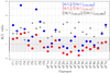 |
Fig. 6 Comparison of the observed M∕L values with the critical ones. The gray circles correspond to the values of
|
![Mathematical equation: $[(M/L)_{\mathrm{crit,vir}}]/$](/articles/aa/full_html/2019/09/aa35260-19/aa35260-19-eq55.png)
![Mathematical equation: $[(M/L)_{\mathrm{crit,O64}}]$](/articles/aa/full_html/2019/09/aa35260-19/aa35260-19-eq56.png)
![Mathematical equation: $[(M/L)]/[(M/L)_{\mathrm{crit,O64}}]$](/articles/aa/full_html/2019/09/aa35260-19/aa35260-19-eq57.png)
![Mathematical equation: $[(M/L)]/[(M/L)_{\mathrm{crit,vir}}]$](/articles/aa/full_html/2019/09/aa35260-19/aa35260-19-eq58.png)
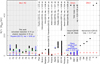 |
Fig. 7 Comparison of the observed M∕L for the filaments F1 to F9 with different low-mass and high-mass star-forming regions. The gray area on the left present the Mon R2 range of values obtained in this work (in black) and by Rayner et al. (2017) (in blue). The gray area located toward the right of the plot present the Orion values. The blue solid bars at the Orion band indicate the M∕L range found in the fibers within each filament. The black bars present the total filament M∕L reported by Bally et al. (1987) and Johnstone & Bally (1999). The red crosses indicate the value of the
|


4.4 Filament kinematics
In this section, we study the kinematic properties of the Mon R2 hub-filament system, with special focus on the line shape properties(Sect. 4.4.1) and the velocity gradients along the filaments (Sect. 4.4.2) and inside the central hub (Sect. 4.5).
4.4.1 Velocity components and linewidths
Most of the main and secondary filaments have a relatively simple velocity structure with one velocity component (see Figs. B.4–B.14). However, a few of them show two velocity components (F6, F7, sF5b, and sF7a). This is similar to the velocity structure observed toward some filaments in low-mass star-forming regions like Taurus, where a number of velocity-coherent, small filaments or fibers have been found (e.g., Hacar et al. 2013). However, other authors (e.g., Zamora-Avilés et al. 2017; Clarke et al. 2018) suggest that it is not clear that fibers are actual objects. Our low angular resolution (~ 25′′, or 0.1 pc), even though it resolves the kinematic structure of the filaments, prevents us from searching for “fiber-like” structures in Mon R2. Higher angular resolution observations with facilities like the Atacama Large Milllimeter/Sub-millimeter Array (ALMA, ALMA Partnership 2015) may help in the search for small-scale substructures.
In order to have a complete image of the kinematical profiles of the filaments, we extracted a number of 13CO and C18O spectra along the filament skeletons. We fit them with Gaussian functions. The whole spectra set and Gaussian fits are shown in Appendix B, while Fig. 8 presents a summary of the main results. Larger linewidths are observed in the hub, very likely as a consequence of filaments merging together and due to the presence of a hot and expanding UC HII region (e.g., Treviño-Morales et al. 2016, see also Sect. 4.5). The filaments have linewidths of 1–2 km s−1 in 13CO, and 0.5–1.5 km s−1 in C18O. Assuming that the gas and dust are thermalized, Tk = Td, the non-thermal velocity dispersion, σNT, can be determined as
![Mathematical equation: \begin{equation*}\sigma_{\mathrm{NT}} = \left[ \left( \frac{ \Delta V }{ \sqrt{8\textrm{ln}2} }\right)^{2} - \left(\frac{k_{\mathrm{B}} T_{\mathrm{k}}}{\mu_{\mathrm{X}}m_{\mathrm{H}}} \right)^{2} \right]^{1/2}, \end{equation*}](/articles/aa/full_html/2019/09/aa35260-19/aa35260-19-eq24.png) (6)
(6)
where ΔV is the observed full width at half maximum, Tk is the kinetic temperature, mH is the mass of the hydrogen atom, and μX is the molecular mass of the a specific molecule (i.e., 29 for 13CO and 30 for C18O). Assuming Tk = Td, all the filaments have Tk between 14 and 18 K (Tables B.1 and B.2), corresponding to a thermal sound speed5 cs (Tk) of 0.23–0.26 km s−1. Using the ratio σNT∕cs(TK), we calculate the Mach number,  , for the main and secondary filaments (see Table B.5) and look for subsonic (
 ), transonic (
 ) and supersonic (
 ) gas motions along them. For the filaments associated with two velocity components (e.g., F6, F7), we estimated the Mach number using the most intense velocity component. Figure 9 (top) presents the distribution of
  of all filaments. There are no significant differences between the main and secondary filaments, with mean (and standard deviation) values of
  (±0.7). Our analysis, therefore, indicates that the main and secondary filaments exhibit transonic non-thermalmotions on average. In Fig. 9 (bottom), we present a comparison of
  with the observed line mass for all the filaments. In the figure it is possible to distinguish a trend suggesting that the filaments that have higher M∕L also have higher
  values (see blue and red lines in Fig. 9).
Finally,we study the variation in linewidth (and velocity dispersion, see bottom panels of Figs. 10 and B.3). We do not find large variations (<0.5 km s−1) in the velocity dispersion along the secondary filaments. In contrast, the velocity dispersion increases along the main filaments when approaching and entering the central hub. Inside the central hub (Rhub < 250′′) the gas has supersonic non-thermal motions on average. It is worth noting that given the moderate spatial resolution of our observations, we cannot exclude the possibility that all our filaments and secondary filaments could contain smaller (subsonic) entities like those observed in other regions (e.g., Orion A: Hacar et al. 2018, Perseus: Hacar et al. 2017b and Taurus: Hacar et al. 2013).
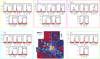 |
Fig. 8 Averaged spectra of the molecules of 13CO (black) and C18O (red) at different positions toward the hub (red box), and the filaments and secondary filaments F1 (pink box), F2 (yellow box), F3 (light-blue box) and, F7 (green box). The positions corresponding to each spectrum are indicated in the central bottom panel. |
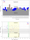 |
Fig. 9 Top: distribution of the Mach number calculated from the 13CO (blue) and C18O (red-gray) velocity dispersion. Bottom: relation between the Mach number and the observed
M∕L. The green area indicates the range of the |


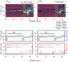 |
Fig. 10 Position-velocity diagrams (top panels) along the skeleton of filament F1 obtained from the 13CO (left) and C18O (right) data cubes. The vertical yellow dashed lines indicate the transition between the hub and the filaments, corresponding to radii 200′′, 250′′ (Rhub), and 300′′. Middle panels: variation in velocity against the offset along the filament in two different manners. The dotted black line corresponds to the velocity obtained at the central pixel that constitutes the skeleton of the filament, while the blue line shows the velocity along the skeleton after averaging over the velocity range shown in the top panels. The green lines indicate the velocity range where most of the emission of the filament resides. Bottom panels: line-width (Δv) of the skeleton’s central pixels along the filaments (in black) and the velocity dispersion calculated from
|

4.4.2 Velocity gradients
In the following, we study the velocity gradients along the filaments by constructing position–velocity (PV) diagrams along all the filament skeletons. The PV diagrams were obtained with the python tool pvextractor6, which generates PV diagrams along any user-defined path or curved line given its spatial coordinates in a position-position-velocity data set. In the PV diagrams we average over ten pixels (corresponding to two beams, or ~ 0.2 pc) in the direction perpendicular to the filament skeleton to enhance the S/N. In this section, we analyze the velocity gradients along the filaments excluding the area located within the hub. The kinematics within the hub are discussed in Sect. 4.5.
Figure 10 (top) shows the PV diagrams along the skeleton of the filament F1 for the 13CO (1 →0) and C18O (1 →0) lines. The PV diagrams for the other filaments are shown in Fig. B.3. Most of the filaments show different velocities at the two ends of the filament, i.e., global velocity gradients. We determine the global velocity gradient of each filament from a linear fit to the velocities along the filament (see middle panels of Figs. 10 and B.3) after excluding the region of the filament located inside Rhub = 250′′. In Table B.5, we list the velocity gradients derived for each filament, which are in the range 0.0–0.8 km s−1 pc−1. Figure 11 shows the distribution of the velocity gradients measured over along filaments.
Some main filaments show significant variations or zig-zag features in the velocity distribution. In particular, filaments F1, F2, F5, and F7 show different velocity gradients in some segments or zones along the filament. These zones are marked in the PV diagrams as ZI to ZIII (see, e.g., Fig. 10). The velocity gradients seen along the defined zones are in the range 0.2–3.0 km s−1 pc−1 (see green and black symbols in Fig. 11). The larger velocity gradients are found in those regions close to the central hub, suggesting that the gas may be accelerating when approaching the center of the potential well. In contrast to the main filaments, the secondary filaments have smooth and constant velocity gradients along them. These velocity patterns have also been observed in numerical simulations of clouds in global collapse (e.g., Gómez & Vázquez-Semadeni 2014).
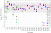 |
Fig. 11 Distribution of the velocity gradients. The blue dots correspond to the values calculated from the 13CO data and thered dots to the values calculated using the C18O data. Theblue and red dotted lines indicates the average values of the gradients. The black triangles (13CO) and green squares (C18O) correspond to the different gradients calculated along the filaments F1, F2, F5, and F7. The Zones (ZI, ZII, and ZIII) labeled in those filaments correspond to those indicated in their respective velocity diagrams (e.g., Fig. 10). |
4.5 Into the hub
As seen in Fig. 4, the filaments extend into the central hub forming a ring structure traced by the DisPerSE filament skeletons. Several velocity components can be distinguished within the hub suggesting a complex structure that remains unresolved due to the limited angular resolution of the 13CO and C18O (1 →0) maps. To explore the morphology and the kinematics of the central hub in more detail, we use the higher angular resolution maps of the 13CO and C18O (2 →1) lines. Figure 12 shows, for different velocity ranges, the superposition of the filament skeletons detected with DisPerSE (white contours) with 13CO and the brightest C18O features. The brightest 13CO (2 →1) emission highlights an elliptical structure (hereafter hub-ring) consistent with the skeleton structure identified from the 13CO (1 →0) data. The hub-ring morphology is also observed in the C18O (2 →1) maps, although it traces an inner layer compared to the 13CO (2 →1) maps. The innermost area of the ring-like structure is, however, devoid of 13CO and C18O emission, suggesting a lack of molecular gas, or a lower column density in the very center. This is likely caused by the interaction of the UC HII region associated with IRS 1 that affects the dynamics, structure, and chemistry of the gas close to the stellar cluster (Pilleri et al. 2012; Treviño-Morales et al. 2016), creating a cavity devoid of gas.
In the following, we describe the kinematics of the gas within the hub-ring. We assume that the gas is falling into the young protostellar cluster while an UC HII region is developing and breaking out the external cocoon. We make use of PV diagrams to search for possible rotation and infall signatures. The right panels in Fig. 13 show the PV diagrams built along the ellipse corresponding to the hub-ring seen in 13CO (red ellipse in Panels A–D in Fig. 13). Panels E and G show the PV dia- grams alongthe hub-ring, while panels H–M show the PV diagrams along the major and minor axes of the ellipse. The gas velocity along the ellipse follows a sinusoidal curve reminiscent of a rotational motion (green dots in Panels E–G). The interpretation of a rotational motion is also supported by the PV diagrams along the major axis with a velocity gradient of about 4 km s−1 pc−1 from east towest (see Panels H–J in Fig. 13). However, the PV diagrams present some features that do not follow the rotational patterns. These features are likely the consequence of the interaction of the young stars with the surrounding gas (bipolar outflows and the UC HII region, Dierickx et al. 2015; Downes et al. 1975; Massi et al. 1985). A velocity gradient, 1–1.5 km s−1 in 0.1–0.2 pc, is observed along the minor axis which is consistent with the presence of infall (see Panels K and M in Fig. 13). The combination of rotation and infall motions suggest that the molecular gas falls into the stellar cluster following a spiral path as seen in the morphology structure of the C18O (2 →1) maps. In Fig. 12, it is possible to distinguish three spiral-filament features flowing into the forming cluster. To look for further support for this scenario, it is interesting to compare the velocity gradient measured in the PV diagram with the free-fall velocity in the gravitational potential created by the stellar cluster. The total mass content in the intermediate -to high-mass IRS 1 to IRS 5 cluster is about 48 M⊙ (Carpenter & Hodapp 2008). We need to add the mass of the population of low-mass near-IR stars. Following Carpenter & Hodapp (2008), there are 371 stars within a circle of R = 1.85 pc. As a first approximation, we can assume that the stellar surface density is uniform, resulting in 154 stars in R < 0.32 pc, and a stellar mass of 77 M⊙ assuming an average stellar mass of 0.5 M⊙. Finally, we should consider the gas mass. The gas density within the HII region is expected to be ~ 100 times lower than in the molecular cloud if we assume thermal pressure equilibrium. However, the fully ionized region has a radius of RHII ~ 0.09 pc, which is much smaller than our ellipse. On the basis of our molecular data, we estimate a mass of ~ 1600 M⊙ within Rhub = 1 pc. Assuming constant volume density, this would imply 43 M⊙ gas mass in the inner 0.32 pc sphere. In total, we would have a mass of 168 M⊙, leading to the free-fall velocity of ~ 2.0 km s−1 at a distance of 0.32 pc (semimajor axis of the ellipse). This free-fall velocity is consistent with the velocity gradients measured along the semiminor axis of the hub-ring. It is important to note that the hub-ring is not completely edge-on, and thus the measured infall velocity is a lower limit. However, the mass content also suffers from significant uncertainty. Therefore, we consider that the proposed infall-rotation scenario is consistent with our observational data. Higher angular resolution observations can better resolve the spiral pattern and provide us with more constraints on the kinematics of the gas in the very center of Mon R2.
It should be noted that similar spiral-like morphologies have been reported by recent observational (see e.g., Galvan-Madrid et al. 2013; Johnston et al. 2015; Liu et al. 2015, 2019; Lin et al. 2016; Schwörer et al. 2019) and theoretical works (see e.g., Gómez & Vázquez-Semadeni 2014; Mapelli 2017) studying OB cluster-forming regions. This indicates that this structure is not a peculiarity of Mon R2, but they are common features in cluster-forming regions and thus it is essential to perform a deeper study of this kind of features.
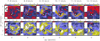 |
Fig. 12 Integrated emission maps in ranges of 1 km s−1 for the C18O 2 →1 line (top panels) and 13CO 2 →1 line (bottom panels). The red lines in the top panels depict the brightest features of the C18O emission, and mark the possible path that the gas follows to reach the stellar cluster, indicated with a white star. The white lines in the bottom panels mark the “skeletons” of the filaments identified by DisPerSE in the 13CO and C18O 1 →0 maps. |
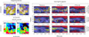 |
Fig. 13 Integrated intensity (panels A and B) and velocity centroid (panels C and D) maps of the C18O and 13CO (2 →1) lines. The red ellipse marks the position of the hub-ring. Panels E–G: PV diagrams clockwise along the hub-ring (starting at the point A of the ellipse) for the 13CO (2 →1), C18O (2 →1) and C18O (1 →0) lines. Panels H and J: PV diagrams along the major axis (from point A to point C). Finally, panels K and M: PV diagrams along the minor axis (from point B to point D). The green dots in panels E–G indicate the velocities associated with the most intense emission along the ellipse, tracing the sinusoidal pattern. The yellow stars in panels H–J show the position of the cluster along the major axis. Finally, the cyan lines in panels K–M mark the strongest velocity gradients along the minor axis. |
5 Discussion
In the previous sections we presented and analyzed the properties of the filaments. In this section we discuss the implications of the kinematical and dynamical properties of the gas along the filamentary network converging into the dense hub.
5.1 Massaccretion rate
The kinematic properties can also give us information on the mass of the accretion flow (Ṁacc) along the filaments of Mon R2. We calculate Ṁacc following Kirk et al. (2013). We consider that the filaments are cylinders with mass M; length, L; and radius, r. They are inclined with respect to the plane of the sky by an angle α and the velocity of the gas along the long axis of the filament is given by V∥. The mass accretion rate, Ṁacc, is given by
 (7)
(7)
where, due to projection effects, Lobs = Lcos(α) and V∥,obs = V∥sin(α). Defining the velocity gradient as ∇V∥,obs = V∥,obs∕Lobs, we can write Eq. (7) as
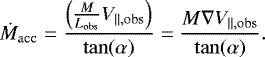 (8)
(8)
As a first approximation, we assume that all the filaments have an inclination of α =45°. In Table B.5, we list, the velocity gradients and the derived mass accretion rates for the filaments in Mon R2 (see also Fig. 14). We determine a mean (standard deviation) accretion rate of 0.72(±0.82) × 10−4 M⊙ yr−1 and 0.17(±0.19) × 10−4 M⊙ yr−1 for the main and secondary filaments, respectively. Changing the inclination angle to 30° (60°) would increase (reduce) the mass accretion rate by a factor of 1.73. Considering that there is no preferred direction, or inclination angle, for the filaments, the measured mass accretion rates indicate that the secondary filaments transport mass to the main filaments at a rate four times lower than the main filaments do to the central hub.
It is important to note that each filament may be distributed around the central core with different inclination angles with respect to the plane of the sky. The angle of the filament can be obtained from
 (9)
(9)
which results in the inclination angle of
 (10)
(10)
Assuming that all the filaments are accreting material onto the hub and have the same velocity gradient, the observed differences can only be due to different inclination angles. Hence, we calculate the average of all the observed velocity gradients to be ⟨∇V∥⟩ = 0.30 km s−1 pc−1 for 13CO and ⟨∇V∥⟩ = 0.35 km s−1 pc−1 for C18O, and consider that this is the velocity gradient at an angle α = 45°. We then determine the angle of each one of the main filaments as α = tan−1(∇V∥,obs∕⟨∇V∥⟩) (see Table B.5). With these angles, we determine the corrected mass accretion rates ( , see Table B.5). Figure 14 (bottom) shows the corrected mass accretion rates for all the filaments. We find a mean (standard deviation) accretion rate of 0.70(± 0.52) × 10−4 M⊙ yr−1 and 0.20(± 0.11) × 10−4 M⊙ yr−1 for the main and secondary filaments, respectively. Considering the eight main filaments that feed the central hub, we determine a total mass accretion rate of 4–7 × 10⁻⁴ M⊙ yr−1. Using Eqs. (9) and (10), it is also possible to determine corrected lengths (Lcorr) for the filaments. We find that these values can be larger than the observed L by a factor of 1.2–2.3, which would result in a decrease of about 35% in the calculated λcl and Mcl parameters. Moreover, the larger values of L result in a decrease of the observed M∕L by a factor of 10–40%.
Compared to other star-forming regions, the mass accretion rates measured along the filaments of Mon R2 (~10−4 M⊙ yr−1) are (i) similar to those found in Serpens (1–3 × 10⁻⁴ M⊙ yr−1, Kirk et al. 2013), Perseus (0.1–0.4 × 10⁻⁴ M⊙ yr−1, Hacar et al. 2017b), and Orion (~ 0.6 × 10⁻⁴ M⊙ yr−1, Rodríguez-Franco et al. 1992; Hacar et al. 2017a); (ii) lower by one order of magnitude than those measured in the DR 21 ridge (~ 10−3 M⊙ yr−1, Schneider et al. 2010); and (iii) higher than those seen in Taurus (0.1–0.9 × 10⁻⁵ M⊙ yr−1, Hacar et al. 2013) and SDC 13 (2–5 × 10⁻⁵M⊙ yr−1, Peretto et al. 2014).
It is important to note that V∥,obs was calculated as an average velocity gradient along the filament. However, it is possible to distinguish changes in the velocity gradients along the filaments F1, F2, F5, and F7. The velocity gradients seen in the different zones (see Figs. 10 and B.3) are in the range 0.2–3.0 km s−1 pc−1 (see green and black markers in Fig. 11), and correspond to Ṁacc of 0.3–3.5 M⊙ yr−1. The largest velocity gradients are found in the vicinity of the hub, i.e., when the filaments reach and enter the hub. This is due to the higher masses (the main filaments gather mass on their trajectories to the hub) and the acceleration of the material when approaching the hub. The behavior seen in filaments F1, F2, F5, and F7 is reminiscent of a gravitational collapse, where a rapid acceleration is expected in the proximity to the potential well, with the velocity varying as R−0.5. In this expression, R is the distance to the center of the potential well which is related to the distance measured in our maps, Rhub, by R = Rhub∕sin(α) with α being the inclination angle relative to the plane of sky. In a rotating cloud, because of the conservation of the angular momentum, the trajectories of the infalling material change from a large-scale radial infall to a rotating flattened structure around the potential well. The rotation within the hub can produce the “zig-zag” variations seen in the PV diagrams. In contrast with the main filaments, the velocity gradients along the secondary filaments show a constant gradient with no significant variations.
We make use of the velocity gradients and the angles derived for each filament to build a 3D vision of the filamentary network in Mon R2. Figure 15 shows a sketch in which we assign a color to each filament depending on its location. We find that the northern (F1) and eastern filaments (F2 to F4) are placed behind the hub (blue-shifted in velocity), while the western filaments (F6 to F9) are placed in front of the hub (red-shifted velocities), with the ones in the north-south direction being less shifted and most likely located close to the plane of thesky. This suggests that the main filaments are located in an extended 2D sheet with an angle of 30° with respectto the plane of the sky, i.e., the eastern side being located behind the plane, and the western side in front of it.
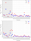 |
Fig. 14 Mass accretion rate along the main and secondary filament considering an inclination of α = 45° (top) and the inclination listed in Table B.5 (bottom). The blue dots correspond to the values calculated from the 13CO parameters (M and ∇V∥obs) and the red ones correspond to the values calculated using the C18O parameters. The gray zone in the plots indicate the values corresponding to the main filaments. |
5.2 Timing a global collapse
In the context of a hub-filament system presenting a global non-isotropic collapse, the gas flows through the filaments to form the central hub. We determine a mass-doubling time of 4–7.5 Myr to build up the current mass of the hub (~ 3000 M⊙) considering the total mass accretion rate of the main filaments (4–7 × 10⁻⁴ M⊙ yr−1). A slightly shorter mass-doubling time (~2.5 Myr) is obtained if we consider the higher mass accretion rates measured in the vicinity of the central hub (~ 12 × 10−4 M⊙ yr−1, see Sect. 5.1). This last value is comparable with the velocity gradients and timescale presented by Rayner et al. (2017) when analyzing only the inner part of the filaments in Mon R2. The mass-doubling time derived from the velocity gradients seen in the filaments is one order of magnitude larger than the free-fall7 time in Mon R2, suggesting a dynamically old region. If the initial density of the cloud is lower, and on the order of ~ 5 × 102 cm−3, the free-fall time is in agreement with the mass-doubling time, suggesting a dynamically young region.
In general, hub-filament systems are likely to be very common in massive collapsing regions as a consequence of the interaction between turbulence and gravitational instabilities. The similarity between observed hub-filament systems with numerical simulations is striking (see e.g., Smith et al. 2009; Gómez & Vázquez-Semadeni 2014; Vázquez-Semadeni et al. 2017; Ballesteros-Paredes et al. 2018; Lee & Hennebelle 2016, 2019). Lee & Hennebelle (2019) present simulations of a collapsing molecular cloud and summarize the main features of the process in (i) a global collapse forming a central stellar cluster, (ii) prominent filamentary structures, and (iii) stars forming along the radial filaments that feed the central cluster. The presence of radial filamentary structures like the one seen in Mon R2 is more prominent in simulations with a low initial density. In this situation (case A of Lee & Hennebelle 2019) the global collapse precedes the formation of most of the stars. Contrary to that, for initially denser clouds (see case C of Lee & Hennebelle 2019), star formation activity is more widespread and the global collapse is less efficient, resulting in a web-like cloud instead of a radially filamentary cloud. A different interpretation for the generation of a radial filamentary structures in a molecular cloud, is presented in Ballesteros-Paredes et al. (2015), where the turbulent crossing time is ~ 6–7 times longer than the sound crossing time (consistent with the obtained in the case A of Lee & Hennebelle 2019). For turbulent crossing times that are much longer or shorter, the morphology can be substantially different (case C of Lee & Hennebelle 2019; Ballesteros-Paredes et al. 2015).
In a recent work Motte et al. (2018) present an evolutionary scheme for the formation of high-mass stars (see their Fig. 8) that follows an empirical scenario qualitatively recalling the global hierarchical collapse and clump-feed accretion scenarios (see Vázquez-Semadeni et al. 2009, 2017; Smith et al. 2009). In this scenario, parsec-scale massive clumps such as ridges (e.g., DR 21) and hub-filament systems (e.g., Mon R2) are the preferred sites for high-mass star formation, and their physical characteristics (velocity, density, and structure) favor a global controlled collapse. The Motte et al. scheme (adapted from Tigé et al. 2017) represents a molecular cloud complex containing a ridge or a hub-filament system with gas flowing through the filaments to the central hub, where a number of massive dense cores/clumps (MDCs, on a 0.1 pc scale) form. During the starless phase (~ 104 yr), MDCs only harbor low-mass prestellar cores. The MDCs become protostellar when hosting a stellar embryo of low mass (~ 3 × 10⁵ yr). Then the protostellar envelopes feed from the gravitationally driven inflows and lead to the formation of high-mass protostars. High-mass protostars become IR bright for stellar embryos with masses higher than 8 M⊙. Finally, the main accretion phase terminates when the stellar UV radiation ionizes the envelope and generates an HII region (in a few 105 –106 yr). The properties of the Mon R2 hub-filament system agree with the morphological description of the scheme presented in Motte et al. (2018). Adapting this evolutionary scheme for the case of Mon R2, we consider that it was necessary for a low initial collapsing mass (dense structure) to reach the current physical and morphological properties of the hub-filament system after ~ 1–2 Myr. Moreover, massive star formation exist in the central hub of Mon R2 for about 105 yr, as determined on the basis of the UC HII region and surrounding PDRs (see Treviño-Morales et al. 2014; Didelon et al. 2015).
Thus far, very few massive star-forming regions have been studied with a detail similar to that presented in this paper (among them: Orionand DR 21, Stutz & Gould 2016; Hacar et al. 2018; Suri et al. 2019). Even though this group is not numerous, it is clear that giant molecular clouds may undergo different types of collapse, most likely related to their initial physical conditions. Mon R2 shows differentiated dynamical properties from the others. While DR 21 and Orion have massive supercritical ridges with high star formation rates, Mon R2 is formed by a network of filaments resembling those in low-mass star-formingregions that converge in a single well-defined gravitational hole where a cluster of massive stars is forming. The formation of the hub and radial filamentary structure has taken more than one million of years. To our knowledge, this is the first massive cloud with these characteristics and thus it is essential to compare it with 3D magneto-hydrodynamic simulations to better understand the star formation process. With its simple geometry and location at only 830 pcfrom the Sun, Mon R2 appears to be an ideal candidate to study the global collapse of a massive cloud.
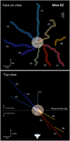 |
Fig. 15 Three-dimensional schematic view of the filamentary structure in Mon R2. Top panel: face-on view of the filaments, as seen in the plane of the sky. Bottom panel: top view of the filaments. Filaments F1 to F4 are placed behind the hub (with blue-shifted velocities), while filaments F6 to F9 are placed in front of the hub (with red-shifted velocities). |
6 Summary and conclusions
In this paper, we studied the stability and the kinematic/dynamic properties of the cluster-forming hub-filament system in the Monoceros R2 molecular cloud. We used large-scale maps of different molecular tracers obtained with the IRAM-30 m telescope, and the H2 column density map derived from Herschel observations. Our main results can be summarized as follows:
-
The large-scale emission seen in 13CO, C18O, HNC, and N2H+ correlates with the Herschel-derived H2 column density. All tracers reveal a hub-filament system in Mon R2.
-
We identified 9 main filaments and 16 secondary filaments in the position–position–velocity data sets. The main filaments converge to the central hub for which we determine a radius Rhub ≈ 1 pc, while the secondary filaments merge into main filaments.
-
We studied the stability of the filaments by determining their line mass (M∕L) and comparing it with the critical line masses of a thermally supported filament and a filament supported by non-thermal motions. The two critical line masses are similar suggesting that thermal pressure and turbulence have similar contributions to the stability of the filaments. The line mass for the main filaments is 30–100 M⊙ pc−1, and is lower for the secondary filaments (12–60 M⊙ pc−1). The main filaments are slightly supercritical, while the secondary filaments are transcritical.
-
We studied the fragmentation of the filaments by comparing the masses and separations of clumps located within the filaments, with the estimates of a fragmenting filament as predicted in two different models: a filament regulated by thermal motions, and a filament with non-thermal support. The observed clump masses (Mcl,obs = 5–35 M⊙) and separations (λcl,obs = 0.25–2.00 pc) are in agreement with a fragmenting properties of a filament if the non-thermal motions are considered.
-
We studied the kinematic properties of the filaments by inspecting the velocity and linewidth values. Most of the filaments have a simple velocity structure with one velocity component, and linewidths of ~0.5–1.5 km s−1. The linewidth increases inside the hub, likely due to the filaments merging together and to presence of a hot and expanding UC HII region. We find subsonic non-thermal motions along the filaments, which become supersonic inside the hub.
-
We measured velocity gradients ≈0.4 km s−1 pc−1 in the filaments of Mon R2, and derived mass accretion rates of ≈0.7 × 10⁻⁴ M⊙ yr−1 and ≈0.2 × 10⁻⁴ M⊙ yr−1 for the main and secondary filaments, respectively. We find significant variations in the velocity of some main filaments, in particular when approaching or entering the hub. The velocity gradients and mass accretion rates of these filaments increase by a factor of a few in the vicinity of the central hub, likely due to an acceleration of the accretion flow when approaching the center of the potential well.
-
We determined that most of the main filaments extend into the central hub forming a ring structure. The kinematics of the hub-ring reveal signs of rotation and infall motions with gas flowing from the external filaments to the central massive cluster following a spiral-like pattern.
-
We constructed a 3D schematic view of the filamentary structure in Mon R2. Filaments F1 to F4 (located to the north and east) are placed behind the hub. Filaments F6 to F9 (located in the south and west) are placed in front of the hub. This scheme suggests that the filaments in Mon R2 may be distributed in a 2D plane with an angle of about 30° with respect to the plane of the sky.
-
Considering that the velocity gradients seen in the main filaments converging to the central hub correspond to infall, we estimate a timescale of about ~2.5 Myr as the necessary time to gather the current mass in the central hub (~3000 M⊙).
Overall, the properties of Mon R2 are in agreement with a scenario of a massive star-forming region that has been formed by a global non-isotropic collapse. The main filaments converge in the central hub from different directions feeding it at an accretion rate of 10−3–10−4 M⊙ yr−1. The mass accretion rates increase along the filaments when approaching or entering in the hub, which may be due to an acceleration of the gas when entering the hub. In a similar way, secondary filaments feed the main filaments at lower mass accretion rates. The main filaments extend in to the central hub forming a ring structure. Within the hub, it is possible to distinguish several velocity components suggesting a complex structure that remains unresolved. The kinematics inside the hub show signs of rotation and infall motions with the gas converging in to the stellar cluster following a spiral like pattern, while the central UC HII region is expanding and breaking out of the surrounding envelope. Thanks to its simple geometry and nearby distance (830 pc), Mon R2 is an ideal candidate to study the global collapse of a massive cloud and the formation process of high-mass stars, combining both high spatial resolution observations and numerical simulations.
Acknowledgements
S.P.T.M. and J.K. acknowledge to the European Union’s Horizon 2020 research and innovation program for funding support given under grant agreement No 639459 (PROMISE). A.F. thanks the Spanish MINECO for funding support from grants AYA2016-75 066-C2-2-P, and ERC under ERC-2013-SyG, G.A. 610 256 NANOCOSMOS. A.S.M. and S.S. thank the Deutsche Forschungsgemeinschaft (DFG) for funding support via the collaborative research grant SFB 956, projects A6 and A4. P.P. acknowledges financial support from the Center National de Etudes Spatiales (CNES). N.S. acknowledges support from the French ANR and the German DFG through the project “GENESIS” (ANR-16-CE92-0035-01/DFG1591/2-1). S.S. acknowledges support from the European Research Council under the Horizon 2020 Framework Program via the ERC Consolidator Grant CSF-648 505. S.G. is funded by the European Research Council under Grant Agreement no. 339 177 (STARLIGHT) of the European Community’s Seventh Framework Programme (FP7/2007-2013). J.R.G. thanks the Spanish MICIU for funding support from grant AYA2017-85 111-P. S.P.T.M. acknowledges to J. Orkisz for useful discussions. We thank the anonymous referee for the constructive comments.
Appendix A Mass and column density
The mass M of the filaments is given by
 (A.1)
(A.1)
where N(H2) is the total column density of the H2 molecule, A is the surface area of the filament and mH is the hydrogen mass. When the mass is determined from a molecular tracer different to H2 (e.g., 13CO, C18O) Eq. (A.1) is written as
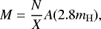 (A.2)
(A.2)
where N is the total molecular column density and X its abundance with respect to H2.
The molecular column density can be determined from observations of a molecular transition from level u (upper) to level l (lower). In particular (see e.g., Estalella & Anglada 1999; Sánchez-Monge 2011), the column density of molecules in the u level (Nu) is related to the optical depth as a function of velocity (τv) by
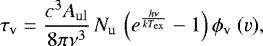 (A.3)
(A.3)
where c is the speed of light, Aul is the Einstein spontaneous emission coefficient, ν is the frequency of the transition, Tex is the excitation temperature, h is the Planck constant, k is the Boltzmann constant and ϕv (v) is the line profile function. The parameter Nu corresponds to the number of molecules in the energy level u (integrated over the path-length dx). The optical depth (τv) can be rewritten in terms of the maximum optical depth (τ0 at the center of theline) and the linewidth (Δv) using
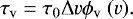 (A.4)
(A.4)
Inserting Eq. (A.4) in Eq. (A.3) and normalizing the line profile to 1, ∫ ϕv (v) = 1, we obtain
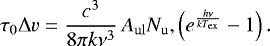 (A.5)
(A.5)
In the Rayleigh–Jeans approximation (hν ≪ kTex), Eq. (A.5) can be written as
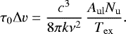 (A.6)
(A.6)
The number of molecules in the energy level u (Nu) is related to the total number of molecules (N) by
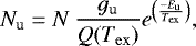 (A.7)
(A.7)
where gu and Eu are the upper state degeneracy and energy, respectively, and Q(Tex) is the partition function defined as the sum over all the posible energy levels. Substituting Eq. (A.7) in Eq. (A.6), we have
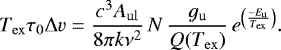 (A.8)
(A.8)
The opacity term in Eq. (A.8) can be written as
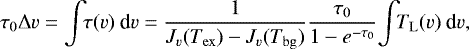 (A.9)
(A.9)
(e.g., Palau et al. 2006). Where Jv(T) is defined as
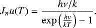 (A.10)
If Jv(Tex) ≫ Tbg, where Tbg is the background temperature, Eq. (A.9) can be written as
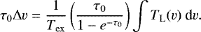 (A.11)
Combining Eqs. (A.8) and (A.11), the total molecular column density N can be written as
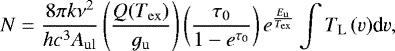 (A.12)
which simplifies to
 (A.13)
in the optically thin scenario (τ ≪ 1).
The partition funtion is  . For linear molecules like CO, the degeneracy and energy of a rotational transition going from level u (described by the quantum number J) to a lower level l (described by the quantum number J − 1) are given by gu = (2J + 1) and Eu = J(J + 1)hB0, where B0 = h∕(8π2I) is the rotational constant of the molecule and I its moment of inertia. Then, the partition function can be written as
 (A.14)
For 13CO and C18O, B0 is 55101.012 MHz and 54891.421 MHz, respectively, and the partition function canbe calculated as Q(Tex) = Tex∕2.644416 K for 13CO, and Q(Tex) = Tex∕2.634358 K for C18O. Applying this to Eq. (A.13), we find that the column density N is
![Mathematical equation: \begin{equation*}\left[\frac{N(^{13}\mathrm{CO})}{\mathrm{cm}^{-2}}\right]=4.69\,{\times}\,10^{13}\left[T_{\mathrm{ex}}\right]e^{\left(\frac{5.3}{T_{\mathrm{ex}}}\right)}\left[\frac{\int T(v)~\textrm{d}v}{\mathrm{K~km~s}^{-1}}\right], \end{equation*}](/articles/aa/full_html/2019/09/aa35260-19/aa35260-19-eq53.png) (A.15)
(A.15)
for the 13CO (1 →0) line, and
![Mathematical equation: \begin{equation*}\left[\frac{N(\mathrm{C^{18}O})}{\mathrm{cm}^{-2}}\right]=4.723\,{\times}\,10^{13}\left[T_{\mathrm{ex}}\right]e^{\left(\frac{5.28}{T_{\mathrm{ex}}}\right)}\left[\frac{\int T(v)~\textrm{d}v}{\mathrm{K~km~s}^{-1}}\right] \end{equation*}](/articles/aa/full_html/2019/09/aa35260-19/aa35260-19-eq54.png) (A.16)
(A.16)
for the C18O (1 →0) line8.
Appendix B Additional figures and tables
In this section, we present additional figures and tables listing the main parameters of the filaments identified in Mon R2.
Figure B.1 shows an abundance map of the main analyzed species 13CO and C18O. These maps have been obtained from the molecular column density maps obtained pixel by pixel using Eqs. (A.15) and (A.16), and the H2 column density map obtained from Herschel (Didelon et al. 2015).
In Fig. B.2, we show the ranges of the observed and predicted masses (top) and separations (bottom) between the clumps obtained from the stability analysis presented in Sect. 4.3. Tables B.1–B.4 list the stability parameters of the main and secondary filaments identified in Mon R2. All the parameters are calculated on basis of the 13CO, C18O, and H2 (derived from dust) molecular emission, following the analysis presented in Appendix A.
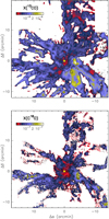 |
Fig. B.1 13CO and C18O abundance maps toward Mon R2. The yellow star at offset (0′′, 0′′) indicates the position of IRS 1. |
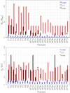 |
Fig. B.2 Masses (top panel) and separation (bottom panel) of clumps within main and secondary filaments. The observed values are marked in black, and the ranges are set from the minimum and maximum values obtained from the different molecular tracers (see Tables B.1–B.4). Theoretical values are marked in blue (following the O64 model) and in red (following the C51 model), see Sect. 4.3. |
Table B.5 lists the kinematic parameters of the filaments derived from the 13CO and C18O emission maps. Figure B.3 shows the position-velocity diagrams along the skeletons of the main and secondary filaments for both 13CO and C18O. Figures B.4 and B.14 show 13CO (black) and C18O (red) spectra along the main filaments. The green solid lines correspond to Gaussian fits. The parameters of the Gaussian functions are listed in Table B.6.
Physical parameters of the main filaments.
Physical parameters of the secondary filaments.
Clumps properties of the main filaments.
Clumps properties of the secondary filaments.
Kinematical parameters of the main and secondary filaments.
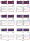 |
Fig. B.3 Position-velocity diagrams along the skeletons of the main and secondary filaments. For each filament there is a set of six plots showing the results for 13CO (left) and C18O (right). The description of the panels and symbols can be found in Fig. 10. |
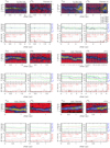 |
Fig. B.3 continued. |
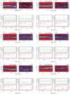 |
Fig. B.3 continued. |
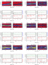 |
Fig. B.3 continued. |
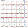 |
Fig. B.4 Spectra of the 13CO (black) and C18O (red) lines. These spectra were extracted along skeleton of the Filament 1. The green solid lines correspond to the Gaussian fits listed in Table B.6. The blue dashed line shows the velocity of 10 km s−1. The corresponding positions for each spectra are indicated in the top left corner of the panels. The positions corresponding to the filaments outside the hub are labeled in black. The positions corresponding to spectra inside the central hub (Rhub = 250″) are in blue. The colored symbols in the panels indicate the positions corresponding with sources identified by Rayner et al. (2017). The pink stars correspond to protostars, the green circles to bound cores, and the red triangles to unbound clumps. The large aqua circles correspond to the sources identified by Sokol et al. (2019). Figures B.5–B.12 show the spectra along the Filaments 2–9 skeleton. Figures B.13 and B.14 show the spectra along the secondary filament skeletons. |
Gaussian fit parameters for offsets along the filaments.
References
- Abreu-Vicente, J., Ragan, S., Kainulainen, J., et al. 2016, A&A, 590, A131 [NASA ADS] [CrossRef] [EDP Sciences] [Google Scholar]
- ALMA Partnership (Fomalont, E. B., et al.) 2015, ApJ, 808, L1 [Google Scholar]
- André, P., Men’shchikov, A., Bontemps, S., et al. 2010, A&A, 518, L102 [NASA ADS] [CrossRef] [EDP Sciences] [Google Scholar]
- André, P., Könyves, V., Arzoumanian, D., & Palmeirim, P. 2014, The Labyrinth of Star Formation (Berlin: Springer Science & Business Media), 36, 225 [NASA ADS] [CrossRef] [Google Scholar]
- Arzoumanian, D., André, P., Didelon, P., et al. 2011, A&A, 529, L6 [Google Scholar]
- Arzoumanian, D., André, P., Könyves, V., et al. 2019, A&A, 621, A42 [NASA ADS] [CrossRef] [EDP Sciences] [Google Scholar]
- Ballesteros-Paredes, J., Hartmann, L. W., Pérez-Goytia, N., & Kuznetsova, A. 2015, MNRAS, 452, 566 [NASA ADS] [CrossRef] [Google Scholar]
- Ballesteros-Paredes, J., Vázquez-Semadeni, E., Palau, A., & Klessen, R. S. 2018, MNRAS, 479, 2112 [NASA ADS] [Google Scholar]
- Bally, J., Langer, W. D., Stark, A. A., & Wilson, R. W. 1987, ApJ, 312, L45 [NASA ADS] [CrossRef] [Google Scholar]
- Berné, O., Fuente, A., Goicoechea, J. R., et al. 2009, ApJ, 706, L160 [NASA ADS] [CrossRef] [Google Scholar]
- Busquet, G., Zhang, Q., Palau, A., et al. 2013, ApJ, 764, L26 [NASA ADS] [CrossRef] [Google Scholar]
- Carpenter, J. M., & Hodapp, K. W. 2008, Handbook of Star-forming Regions (San Francisco: ASP Monograph Publications), I, 4, 899 [NASA ADS] [Google Scholar]
- Carter, M., Lazareff, B., Maier, D., et al. 2012, A&A, 538, A89 [NASA ADS] [CrossRef] [EDP Sciences] [Google Scholar]
- Chandrasekhar, S. 1951, Phil. Trans. R. Soc. London Ser. A, 210, 26 [NASA ADS] [CrossRef] [MathSciNet] [Google Scholar]
- Clarke, S. D., Whitworth, A. P., & Hubber, D. A. 2016, MNRAS, 458, 319 [NASA ADS] [CrossRef] [Google Scholar]
- Clarke, S. D., Whitworth, A. P., Duarte-Cabral, A., & Hubber, D. A. 2017, MNRAS, 468, 2489 [NASA ADS] [CrossRef] [Google Scholar]
- Clarke, S. D., Whitworth, A. P., Spowage, R. L., et al. 2018, MNRAS, 479, 1722 [NASA ADS] [CrossRef] [Google Scholar]
- Clarke, S. D., Williams, G. M., Ibáñez-Mejía, J. C., et al. 2019, MNRAS, 484, 4024 [NASA ADS] [CrossRef] [Google Scholar]
- Chira, R.-A., Kainulainen, J., Ibáñez-Mejía, J. C., Henning, T., & Mac Low, M.-M. 2018, A&A, 610, A62 [NASA ADS] [CrossRef] [EDP Sciences] [Google Scholar]
- Choi, M., Evans, N. J., II, Tafalla, M., & Bachiller, R. 2000, ApJ, 538, 738 [NASA ADS] [CrossRef] [Google Scholar]
- Csengeri, T., Bontemps, S., Schneider, N., & Motte, F. 2011, Computational Star Formation, IAU Symp., 270, 53 [NASA ADS] [Google Scholar]
- Didelon, P., Motte, F., Tremblin, P., et al. 2015, A&A, 584, A4 [NASA ADS] [CrossRef] [EDP Sciences] [Google Scholar]
- Dierickx, M., Jiménez-Serra, I., Rivilla, V. M., & Zhang, Q. 2015, ApJ, 803, 89 [NASA ADS] [CrossRef] [Google Scholar]
- Downes, D., Winnberg, A., Goss, W. M., & Johansson, L. E. B. 1975, A&A, 44, 243 [NASA ADS] [Google Scholar]
- Estalella, R., & Anglada, G. (1999). Introdución a la Física del Medio Interestelar (Barcelona: Edicions Universitat de Barcelona) [Google Scholar]
- Fehér, O., Tóth, L. V., Ward-Thompson, D., et al. 2016, A&A, 590, A75 [NASA ADS] [CrossRef] [EDP Sciences] [Google Scholar]
- Fernández-López, M., Arce, H. G., Looney, L., et al. 2014, ApJ, 790, L19 [NASA ADS] [CrossRef] [Google Scholar]
- Fiege, J. D., & Pudritz, R. E. 2000a, MNRAS, 311, 85 [NASA ADS] [CrossRef] [Google Scholar]
- Fiege, J. D., & Pudritz, R. E. 2000b, MNRAS, 311, 105 [NASA ADS] [CrossRef] [Google Scholar]
- Fischera, J., & Martin, P. G. 2012, A&A, 542, A77 [NASA ADS] [CrossRef] [EDP Sciences] [Google Scholar]
- Fuente, A., Berné, O., Cernicharo, J., et al. 2010, A&A, 521, L23 [NASA ADS] [CrossRef] [EDP Sciences] [Google Scholar]
- Galván-Madrid, R., Liu, H. B., Zhang, Z.-Y., et al. 2013, ApJ, 779, 121 [NASA ADS] [CrossRef] [Google Scholar]
- Giannakopoulou, J., Fich, M., & Wilson, C. D. 1996, BAAS, 28, 894 [NASA ADS] [Google Scholar]
- Giannakopoulou, J., Mitchell, G. F., Hasegawa, T. I., Matthews, H. E., & Maillard, J.-P. 1997, ApJ, 487, 346 [NASA ADS] [CrossRef] [Google Scholar]
- Ginard, D., González-García, M., Fuente, A., et al. 2012, A&A, 543, A27 [NASA ADS] [CrossRef] [EDP Sciences] [Google Scholar]
- Gómez, G, & Vázquez-Semadeni, E. 2014, ApJ, 791, 124 [NASA ADS] [CrossRef] [Google Scholar]
- Hacar, A., Tafalla, M., Kauffmann, J., & Kovács, A. 2013, A&A, 554, A55 [NASA ADS] [CrossRef] [EDP Sciences] [Google Scholar]
- Hacar, A., Kainulainen, J., Tafalla, M., Beuther, H., & Alves, J. 2016, A&A, 587, A97 [NASA ADS] [CrossRef] [EDP Sciences] [Google Scholar]
- Hacar, A., Tafalla, M., & Alves, J. 2017b, A&A, 606, A123 [NASA ADS] [CrossRef] [EDP Sciences] [Google Scholar]
- Hacar, A., Alves, J., Tafalla, M., & Goicoechea, J. R. 2017a, A&A, 602, L2 [NASA ADS] [CrossRef] [EDP Sciences] [Google Scholar]
- Hacar, A., Tafalla, M., Forbrich, J., et al. 2018, A&A, 610, A77 [NASA ADS] [CrossRef] [EDP Sciences] [Google Scholar]
- Heitsch, F. 2013a, ApJ, 769, 115 [NASA ADS] [CrossRef] [Google Scholar]
- Heitsch, F. 2013b, ApJ, 776, 62 [NASA ADS] [CrossRef] [Google Scholar]
- Hennemann, M., Motte, F., Schneider, N., et al. 2012, A&A, 543, L3 [NASA ADS] [CrossRef] [EDP Sciences] [Google Scholar]
- Henshaw, J. D., Caselli, P., Fontani, F., Jiménez-Serra, I., & Tan, J. C. 2014, MNRAS, 440, 2860 [NASA ADS] [CrossRef] [Google Scholar]
- Henshaw, J. D., Jiménez-Serra, I., Longmore, S. N., et al. 2017, MNRAS, 464, L31 [NASA ADS] [CrossRef] [Google Scholar]
- Herbst, W., & Racine, R. 1976, AJ, 81, 840 [NASA ADS] [CrossRef] [Google Scholar]
- Inutsuka, S.-I., & Miyama, S. M. 1992, ApJ, 388, 392 [NASA ADS] [CrossRef] [Google Scholar]
- Inutsuka, S.-i.,& Miyama, S. M. 1997, ApJ, 480, 681 [NASA ADS] [CrossRef] [Google Scholar]
- Jaffe, D. T., Zhu, Q., Lacy, J. H., & Richter, M. 2003, ApJ, 596, 1053 [NASA ADS] [CrossRef] [Google Scholar]
- Johnston, K. G., Robitaille, T. P., Beuther, H., et al. 2015, ApJ, 813, L19 [NASA ADS] [CrossRef] [Google Scholar]
- Johnstone, D.,& Bally, J. 1999, ApJ, 510, L49 [NASA ADS] [CrossRef] [Google Scholar]
- Kainulainen, J., Hacar, A., Alves, J., et al. 2016, A&A, 586, A27 [NASA ADS] [CrossRef] [EDP Sciences] [Google Scholar]
- Kainulainen, J., Stutz, A. M., Stanke, T., et al. 2017, A&A, 600, A141 [NASA ADS] [CrossRef] [EDP Sciences] [Google Scholar]
- Kirk, H., Myers, P. C., Bourke, T. L., et al. 2013, ApJ, 766, 115 [NASA ADS] [CrossRef] [Google Scholar]
- Kirk, H., Klassen, M., Pudritz, R., & Pillsworth, S. 2015, ApJ, 802, 75 [NASA ADS] [CrossRef] [Google Scholar]
- Klessen, R. S., Heitsch, F., & Mac Low, M.-M. 2000, ApJ, 535, 887 [NASA ADS] [CrossRef] [Google Scholar]
- Klein, B., Hochgürtel, S., Krämer, I., et al. 2012, A&A, 542, L3 [NASA ADS] [CrossRef] [EDP Sciences] [Google Scholar]
- Kuznetsova, A., Hartmann, L., & Ballesteros-Paredes, J. 2018, MNRAS, 473, 2372 [NASA ADS] [CrossRef] [Google Scholar]
- Larson, R. B. 1985, MNRAS, 214, 379 [NASA ADS] [Google Scholar]
- Lasker, B. M., Sturch, C. R., McLean, B. J., et al. 1990, AJ, 99, 2019 [NASA ADS] [CrossRef] [Google Scholar]
- Lee, Y.-N., & Hennebelle, P. 2016, A&A, 591, A30 [NASA ADS] [CrossRef] [EDP Sciences] [Google Scholar]
- Lee, Y.-N., & Hennebelle, P. 2019, A&A, 622, A125 [NASA ADS] [CrossRef] [EDP Sciences] [Google Scholar]
- Lin, Y., Liu, H. B., Li, D., et al. 2016, ApJ, 828, 32 [NASA ADS] [CrossRef] [Google Scholar]
- Liu, H. B., Jiménez-Serra, I., Ho, P. T. P., et al. 2012, ApJ, 756, 10 [NASA ADS] [CrossRef] [Google Scholar]
- Liu, H. B., Galván-Madrid, R., Jiménez-Serra, I., et al. 2015, ApJ, 804, 37 [NASA ADS] [CrossRef] [Google Scholar]
- Liu, H. B., Chen, H.-R. V., Román-Zú niga, C. G., et al. 2019, ApJ, 871, 185 [NASA ADS] [CrossRef] [Google Scholar]
- Loren, R. B. 1989a, ApJ, 338, 902 [NASA ADS] [CrossRef] [Google Scholar]
- Loren, R. B. 1989b, ApJ, 338, 925 [NASA ADS] [CrossRef] [Google Scholar]
- Louvet, F., Motte, F., Hennebelle, P., et al. 2014, A&A, 570, A15 [NASA ADS] [CrossRef] [EDP Sciences] [Google Scholar]
- Nagai, T., Inutsuka, S.-i., & Miyama, S. M. 1998, ApJ, 506, 306 [NASA ADS] [CrossRef] [Google Scholar]
- Mapelli, M. 2017, MNRAS, 467, 3255 [NASA ADS] [CrossRef] [Google Scholar]
- Martí, J., Luque-Escamilla, P. L., Mu noz-Arjonilla, A. J., et al. 2013, A&A, 556, A131 [NASA ADS] [CrossRef] [EDP Sciences] [Google Scholar]
- Massi, M., Felli, M., & Simon, M. 1985, A&A, 152, 387 [NASA ADS] [Google Scholar]
- Myers, P. C. 2009, ApJ, 700, 1609 [NASA ADS] [CrossRef] [EDP Sciences] [Google Scholar]
- Miyama, S. M., Narita, S., & Hayashi, C. 1987a, Prog. Theor. Exp. Phys., 78, 1051 [NASA ADS] [CrossRef] [Google Scholar]
- Miyama, S. M., Narita, S., & Hayashi, C. 1987b, Prog. Theor. Exp. Phys., 78, 1273 [NASA ADS] [CrossRef] [Google Scholar]
- Megeath, S. T., Gutermuth, R., Muzerolle, J., et al. 2012, AJ, 144, 192 [NASA ADS] [CrossRef] [Google Scholar]
- Molinari, S., Swinyard, B., Bally, J., et al. 2010, A&A, 518, L100 [NASA ADS] [CrossRef] [EDP Sciences] [Google Scholar]
- Molina, F. Z., Glover, S. C. O., Federrath, C., & Klessen, R. S. 2012, MNRAS, 423, 2680 [NASA ADS] [CrossRef] [Google Scholar]
- Motte, F., Bontemps, S., & Louvet, F. 2018, ARA&A, 56, 41 [NASA ADS] [CrossRef] [Google Scholar]
- Ostriker, J., 1964, ApJ, 140, 1067 [NASA ADS] [CrossRef] [Google Scholar]
- Palau, A., Ho,P. T. P., Zhang, Q., et al. 2006, ApJ, 636, L137 [NASA ADS] [CrossRef] [Google Scholar]
- Palmeirim, P., André, P., Kirk, J., et al. 2013, A&A, 550, A38 [NASA ADS] [CrossRef] [EDP Sciences] [Google Scholar]
- Panopoulou, G. V., Psaradaki, I., Skalidis, R., Tassis, K., & Andrews, J. J. 2017, MNRAS, 466, 2529 [NASA ADS] [CrossRef] [Google Scholar]
- Peretto, N., Fuller, G. A., Duarte-Cabral, A., et al. 2013, A&A, 555, A112 [NASA ADS] [CrossRef] [EDP Sciences] [Google Scholar]
- Peretto, N., Fuller, G. A., André, P., et al. 2014, A&A, 561, A83 [NASA ADS] [CrossRef] [EDP Sciences] [Google Scholar]
- Pilleri, P., Fuente, A., Cernicharo, J., et al. 2012, A&A, 544, A110 [NASA ADS] [CrossRef] [EDP Sciences] [Google Scholar]
- Pilleri, P., Treviño-Morales, S., Fuente, A., et al. 2013, A&A, 554, A87 [NASA ADS] [CrossRef] [EDP Sciences] [Google Scholar]
- Pilleri, P., Fuente, A., Gerin, M., et al. 2014, A&A, 561, A69 [NASA ADS] [CrossRef] [EDP Sciences] [Google Scholar]
- Pineda, J. L., Goldsmith, P. F., Chapman, N. L., et al. 2011, EAS Pub. Ser., 52, 157 [CrossRef] [Google Scholar]
- Pety, J., Teyssier, D., Fossé, D., et al. 2005, A&A, 435, 885 [NASA ADS] [CrossRef] [EDP Sciences] [Google Scholar]
- Pokhrel, R., Gutermuth, R., Ali, B., et al. 2016, MNRAS, 461, 22 [NASA ADS] [CrossRef] [PubMed] [Google Scholar]
- Pokhrel, R., Myers, P. C., Dunham, M. M., et al. 2018, ApJ, 853, 5 [NASA ADS] [CrossRef] [Google Scholar]
- Rayner, T. S. M., Griffin, M. J., Schneider, N., et al. 2017, A&A, 607, A22 [NASA ADS] [CrossRef] [EDP Sciences] [Google Scholar]
- Recchi, S., Hacar, A., & Palestini, A. 2014, MNRAS, 444, 1775 [NASA ADS] [CrossRef] [Google Scholar]
- Rizzo, J. R., Fuente, A., Rodríguez-Franco, A., & García-Burillo, S. 2003, ApJ, 597, L153 [NASA ADS] [CrossRef] [Google Scholar]
- Rodríguez-Franco, A., Martín-Pintado, J., Gómez-Gonzalez, J., & Planesas, P. 1992, A&A, 264, 592 [NASA ADS] [Google Scholar]
- Sánchez-Monge, Á., 2011, PhD Thesis, Universitat de Barcelona, Spain [Google Scholar]
- Sánchez-Monge, Á., Beltrán, M. T., Cesaroni, R., et al. 2014, A&A, 569, A11 [NASA ADS] [CrossRef] [EDP Sciences] [Google Scholar]
- Schneider, S., & Elmegreen, B. G. 1979, ApJS, 41, 87 [NASA ADS] [CrossRef] [Google Scholar]
- Schneider, N., Csengeri, T., Bontemps, S., et al. 2010, A&A, 520, A49 [NASA ADS] [CrossRef] [EDP Sciences] [Google Scholar]
- Schneider, N., Csengeri, T., Hennemann, M., et al. 2012, A&A, 540, L11 [NASA ADS] [CrossRef] [EDP Sciences] [Google Scholar]
- Schwörer, A., Sánchez-Monge, Á., Schilke, P., et al. 2019, A&A, 628, A6 [NASA ADS] [CrossRef] [EDP Sciences] [Google Scholar]
- Seifried, D., & Walch, S. 2015, MNRAS, 452, 2410 [NASA ADS] [CrossRef] [Google Scholar]
- Seifried, D., & Walch, S. 2016, MNRAS, 459, L11 [NASA ADS] [CrossRef] [Google Scholar]
- Seifried, D., Sánchez-Monge, Á., Suri, S., & Walch, S. 2017, MNRAS, 467, 4467 [NASA ADS] [CrossRef] [Google Scholar]
- Skrutskie, M. F., Cutri, R. M., Stiening, R., et al. 2006, AJ, 131, 1163 [NASA ADS] [CrossRef] [Google Scholar]
- Smith, R. J., Longmore, S, Bonnell, I. 2009, MNRAS, 400, 1775 [Google Scholar]
- Smith, R. J., Glover, S. C. O., & Klessen, R. S. 2014, MNRAS, 445, 2900 [NASA ADS] [CrossRef] [Google Scholar]
- Sokol, A. D., Gutermuth, R. A., Pokhrel, R., et al. 2019, MNRAS, 483, 407 [NASA ADS] [CrossRef] [Google Scholar]
- Sousbie, T. 2011, MNRAS, 414, 350 [NASA ADS] [CrossRef] [Google Scholar]
- Stutz, A. M., & Gould, A. 2016, A&A, 590, A2 [NASA ADS] [CrossRef] [EDP Sciences] [Google Scholar]
- Stutz, A. M., Tobin, J. J., Stanke, T., et al. 2013, ApJ, 767, 36 [NASA ADS] [CrossRef] [Google Scholar]
- Suri, S. T., Sanchez-Monge, A., Schilke, P., et al. 2019, A&A, 623, A142 [NASA ADS] [CrossRef] [EDP Sciences] [Google Scholar]
- Tackenberg, J., Beuther, H., Henning, T., et al. 2014, A&A, 565, A101 [NASA ADS] [CrossRef] [EDP Sciences] [Google Scholar]
- Tafalla, M., & Hacar, A. 2015, A&A, 574, A104 [NASA ADS] [CrossRef] [EDP Sciences] [Google Scholar]
- Thronson, H. A., Jr. Gatley, I., Harvey, P. M., Sellgren, K., & Werner, M. W. 1980, ApJ, 237, 66 [NASA ADS] [CrossRef] [Google Scholar]
- Tigé, J., Motte, F., Russeil, D., et al. 2017, A&A, 602, A77 [NASA ADS] [CrossRef] [EDP Sciences] [Google Scholar]
- Treviño-Morales, 2016, PhD Thesis, Universidad de Granada, Spain [Google Scholar]
- Treviño-Morales, S. P., Pilleri, P., Fuente, A., et al. 2014, A&A, 569, A19 [NASA ADS] [CrossRef] [EDP Sciences] [Google Scholar]
- Treviño-Morales, S. P., Fuente, A., Sánchez-Monge, Á., et al. 2016, A&A, 593, L12 [NASA ADS] [CrossRef] [EDP Sciences] [Google Scholar]
- Vázquez-Semadeni, E., Gómez, G. C., Jappsen, A. K., Ballesteros-Paredes, J., & Klessen, R. S. 2009, ApJ, 707, 1023, 1033 [Google Scholar]
- Vázquez-Semadeni, E., González-Samaniego, A., Colín, P. 2017, MNRAS, 467, 1313 [Google Scholar]
- Wang, K., Zhang, Q., Wu, Y., & Zhang, H. 2011, ApJ, 735, 64 [NASA ADS] [CrossRef] [Google Scholar]
- Wang, K., Zhang, Q., Testi, L., et al. 2014, MNRAS, 439, 3275 [NASA ADS] [CrossRef] [Google Scholar]
- Williams, G. M., Peretto, N., Avison, A., Duarte-Cabral, A., & Fuller, G. A. 2018, A&A, 613, A11 [NASA ADS] [CrossRef] [EDP Sciences] [Google Scholar]
- Zamora-Avilés, M., Ballesteros-Paredes, J., & Hartmann, L. W. 2017, MNRAS, 472, 647 [NASA ADS] [CrossRef] [Google Scholar]
- Zhu, Q.-F., Lacy, J. H., Jaffe, D. T., Richter, M. J., & Greathouse, T. K. 2005, ApJ, 631, 381 [NASA ADS] [CrossRef] [Google Scholar]
- Zhu, Q.-F., Lacy, J. H., Jaffe, D. T., Richter, M. J., & Greathouse, T. K. 2008, ApJS, 177, 584 [NASA ADS] [CrossRef] [Google Scholar]
Under the project numbers 027-14, 035-15 and D03-16; PI: A. Fuente and S. P. Treviño-Morales.
The atmospheric opacity τ at 225 GHz is calculated from the expression τ(225) = 0.058 × pwv + 0.004.
See http://www.iram.fr/IRAMFR/GILDAS for information on the G’ILDAS software.
The nomenclature in this work was chosen to be consistent with the previous analysis presented in Treviño-Morales (2016). The correspondence between our nomenclature and that adopted by Rayner et al. (2017) can be found in Fig. 7.
The thermal sound speed, 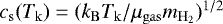 , was calculated assuming an average molecular mass of μgas = 2.7.
The python package pvextractor is freely available at http://keflavich.gitHub.io/pvextractor
Considering the gas density of ~104 cm−3
for Mon R2, the free-fall time (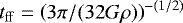 ) is ~3 × 10⁵ yr.
We use ν10 = 110.2013541 GHz, Aul = 6.338 × 10⁻⁸ s−1, gu = 3 for 13CO (1 →0), and ν10 = 109.7821734 GHz, Aul = 6.266 × 10⁻⁸ s−1, gu = 3 for C18O (1 →0). Values reported in the Cologne Database for Molecular Spectroscopy (CDMS, https://cdms.astro.uni-koeln.de/classic/entries/).
All Tables
All Figures
|
Fig. 1 Left: three-color image of the Mon R2 cluster-forming hub-filaments system. Red: H2 column density map derived from Herschel SPIRE and PACS observations (Didelon et al. 2015), green: 1.65 μm band of the Two Micron All Sky Survey (Skrutskie et al. 2006), and blue: 560 nm band of the Digitalized Sky Survey (Lasker et al. 1990). Center: Herschel H2 column density (in cm−2, Didelon et al. 2015). The black polygon shows the area surveyed with the IRAM-30 m telescope, while the white box corresponds to the inner 0.7 pc × 0.7 pc around the central hub and zoomed in the right panel. Right: Herschel H2 column density (in cm−2) of the central hub of Mon R2. Gray contours show the H13CO+ (3 →2) emission tracing the high-density molecular gas (Treviño-Morales et al. 2014). The red star gives the position of IRS 1 (with coordinates α(J2000) = 06h 07m 46.2s, δ(J2000) = − 06°23′08.3″). White stars indicate the positions of infrared sources. The white circle indicates the beam size of the IRAM-30 m telescope at 100 GHz(see Sect. 2). The colored symbols are the sources identified by Rayner et al. (2017): pink stars are protostars, green circles are bound clumps, and red triangles are unbound clumps. |
| In the text | |
|
Fig. 2 Spectra averaged over an area of 0.7 pc × 0.7 pc centered at the position of IRS 1 (corresponding to the area shown in Fig. 1, right). The blue dotted vertical line indicates the source velocity (vLSR = 10 km s−1). The red dashed vertical lines indicate the velocity range where the S∕N is above 3σ for the molecular emission. These ranges are used to generate the integrated intensity maps presented in Fig. 3. The velocity ranges correspond to 5–18 km s−1 for 13CO, 7–15 km s−1 for C18O, 6–14 km s−1 for HNC, and 7–12 km s−1 for N2 H+. |
| In the text | |
|
Fig. 3 Left column panels: integrated intensity maps over the whole surveyed area for the (1 →0) transition lines of the 13CO, C18O, HNC and N2H+ molecules. Middle column: velocity centroid. Right column panels: linewidth. The maps were produced by computing the zero-order (left), first-order (middle) and second-order (right) moments in the velocity range defined in Fig. 2. The yellow labels and the dotted lines indicate the main features identified in the region. The red star at (0′′,0′′) offset gives the position of IRS 1. |
| In the text | |
|
Fig. 4 Top panels: H2 column density (left) and dust temperature (right) maps from Herschel (Didelon et al. 2015). Middle panels: 13CO (left) and C18O (right) column density maps. Bottom panels: velocity centroid for 13CO (left) and C18O (right). The “skeleton” of identified filaments are marked with solid white, black, or yellow lines. The black and white circles correspond to the radii at 200′′, 250′′, and 300′′ (transition between thehub and the filaments, see Fig. 5). The white circles in the top right panel shows sources identified bySokol et al. (2019); the colored symbols show the sources identified by Rayner et al. (2017). |
| In the text | |
|
Fig. 5 Azimuthally averaged mass and surface density derived from the 13CO (top) and C18O (bottom) column density maps. From left to right: each column shows (i) radially integratedmass, (ii) radially integrated mass divided by the area of the circle with radius Rcir (i.e., radially integrated surface density), (iii) concentric annular mass, (iv) concentric annular surface density. The radially integrated mass and surface density were calculated within circles of radius Rcir centered on IRS 1 from R = 25″ (~ 0.1 pc) to R = 600″ (~ 2.4 pc). The concentric annular mass and surface density were calculated within concentric rings of radius Rring =Rcir,out − Rcir,in = 36″ (corresponding to the Herschel beam size). In order to do a direct comparison of the profiles, the x-axis in the concentric annular mass and surface density profiles correspond to Rcir,out. The yellow dotted lines indicate the different slopes in the surface density profiles. The light gray zone indicates the transition between the hub and the filaments, from 200′′ to 300′′. The dark gray area marks the central hub with Rhub = 250” = 1 pc. |
| In the text | |
|
Fig. 6 Comparison of the observed M∕L values with the critical ones. The gray circles correspond to the values of
|
| In the text | |
|
Fig. 7 Comparison of the observed M∕L for the filaments F1 to F9 with different low-mass and high-mass star-forming regions. The gray area on the left present the Mon R2 range of values obtained in this work (in black) and by Rayner et al. (2017) (in blue). The gray area located toward the right of the plot present the Orion values. The blue solid bars at the Orion band indicate the M∕L range found in the fibers within each filament. The black bars present the total filament M∕L reported by Bally et al. (1987) and Johnstone & Bally (1999). The red crosses indicate the value of the
|
| In the text | |
|
Fig. 8 Averaged spectra of the molecules of 13CO (black) and C18O (red) at different positions toward the hub (red box), and the filaments and secondary filaments F1 (pink box), F2 (yellow box), F3 (light-blue box) and, F7 (green box). The positions corresponding to each spectrum are indicated in the central bottom panel. |
| In the text | |
|
Fig. 9 Top: distribution of the Mach number calculated from the 13CO (blue) and C18O (red-gray) velocity dispersion. Bottom: relation between the Mach number and the observed
M∕L. The green area indicates the range of the |
| In the text | |
|
Fig. 10 Position-velocity diagrams (top panels) along the skeleton of filament F1 obtained from the 13CO (left) and C18O (right) data cubes. The vertical yellow dashed lines indicate the transition between the hub and the filaments, corresponding to radii 200′′, 250′′ (Rhub), and 300′′. Middle panels: variation in velocity against the offset along the filament in two different manners. The dotted black line corresponds to the velocity obtained at the central pixel that constitutes the skeleton of the filament, while the blue line shows the velocity along the skeleton after averaging over the velocity range shown in the top panels. The green lines indicate the velocity range where most of the emission of the filament resides. Bottom panels: line-width (Δv) of the skeleton’s central pixels along the filaments (in black) and the velocity dispersion calculated from
|
| In the text | |
|
Fig. 11 Distribution of the velocity gradients. The blue dots correspond to the values calculated from the 13CO data and thered dots to the values calculated using the C18O data. Theblue and red dotted lines indicates the average values of the gradients. The black triangles (13CO) and green squares (C18O) correspond to the different gradients calculated along the filaments F1, F2, F5, and F7. The Zones (ZI, ZII, and ZIII) labeled in those filaments correspond to those indicated in their respective velocity diagrams (e.g., Fig. 10). |
| In the text | |
|
Fig. 12 Integrated emission maps in ranges of 1 km s−1 for the C18O 2 →1 line (top panels) and 13CO 2 →1 line (bottom panels). The red lines in the top panels depict the brightest features of the C18O emission, and mark the possible path that the gas follows to reach the stellar cluster, indicated with a white star. The white lines in the bottom panels mark the “skeletons” of the filaments identified by DisPerSE in the 13CO and C18O 1 →0 maps. |
| In the text | |
|
Fig. 13 Integrated intensity (panels A and B) and velocity centroid (panels C and D) maps of the C18O and 13CO (2 →1) lines. The red ellipse marks the position of the hub-ring. Panels E–G: PV diagrams clockwise along the hub-ring (starting at the point A of the ellipse) for the 13CO (2 →1), C18O (2 →1) and C18O (1 →0) lines. Panels H and J: PV diagrams along the major axis (from point A to point C). Finally, panels K and M: PV diagrams along the minor axis (from point B to point D). The green dots in panels E–G indicate the velocities associated with the most intense emission along the ellipse, tracing the sinusoidal pattern. The yellow stars in panels H–J show the position of the cluster along the major axis. Finally, the cyan lines in panels K–M mark the strongest velocity gradients along the minor axis. |
| In the text | |
|
Fig. 14 Mass accretion rate along the main and secondary filament considering an inclination of α = 45° (top) and the inclination listed in Table B.5 (bottom). The blue dots correspond to the values calculated from the 13CO parameters (M and ∇V∥obs) and the red ones correspond to the values calculated using the C18O parameters. The gray zone in the plots indicate the values corresponding to the main filaments. |
| In the text | |
|
Fig. 15 Three-dimensional schematic view of the filamentary structure in Mon R2. Top panel: face-on view of the filaments, as seen in the plane of the sky. Bottom panel: top view of the filaments. Filaments F1 to F4 are placed behind the hub (with blue-shifted velocities), while filaments F6 to F9 are placed in front of the hub (with red-shifted velocities). |
| In the text | |
|
Fig. B.1 13CO and C18O abundance maps toward Mon R2. The yellow star at offset (0′′, 0′′) indicates the position of IRS 1. |
| In the text | |
|
Fig. B.2 Masses (top panel) and separation (bottom panel) of clumps within main and secondary filaments. The observed values are marked in black, and the ranges are set from the minimum and maximum values obtained from the different molecular tracers (see Tables B.1–B.4). Theoretical values are marked in blue (following the O64 model) and in red (following the C51 model), see Sect. 4.3. |
| In the text | |
|
Fig. B.3 Position-velocity diagrams along the skeletons of the main and secondary filaments. For each filament there is a set of six plots showing the results for 13CO (left) and C18O (right). The description of the panels and symbols can be found in Fig. 10. |
| In the text | |
|
Fig. B.3 continued. |
| In the text | |
|
Fig. B.3 continued. |
| In the text | |
|
Fig. B.3 continued. |
| In the text | |
|
Fig. B.4 Spectra of the 13CO (black) and C18O (red) lines. These spectra were extracted along skeleton of the Filament 1. The green solid lines correspond to the Gaussian fits listed in Table B.6. The blue dashed line shows the velocity of 10 km s−1. The corresponding positions for each spectra are indicated in the top left corner of the panels. The positions corresponding to the filaments outside the hub are labeled in black. The positions corresponding to spectra inside the central hub (Rhub = 250″) are in blue. The colored symbols in the panels indicate the positions corresponding with sources identified by Rayner et al. (2017). The pink stars correspond to protostars, the green circles to bound cores, and the red triangles to unbound clumps. The large aqua circles correspond to the sources identified by Sokol et al. (2019). Figures B.5–B.12 show the spectra along the Filaments 2–9 skeleton. Figures B.13 and B.14 show the spectra along the secondary filament skeletons. |
| In the text | |
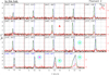 |
Fig. B.5 Same as Fig. B.4, but for main filament F2. |
| In the text | |
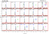 |
Fig. B.6 Same as Fig. B.4, but for main filament F3. |
| In the text | |
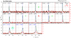 |
Fig. B.7 Same as Fig. B.4, but for main filament F4. |
| In the text | |
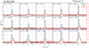 |
Fig. B.8 Same as Fig. B.4, but for main filament F5. |
| In the text | |
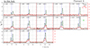 |
Fig. B.9 Same as Fig. B.4, but for main filament F6. |
| In the text | |
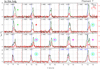 |
Fig. B.10 Same as Fig. B.4, but for main filament F7. |
| In the text | |
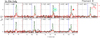 |
Fig. B.11 Same as Fig. B.4, but for main filament F8. |
| In the text | |
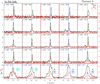 |
Fig. B.12 Same as Fig. B.4, but for main filament F9. |
| In the text | |
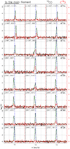 |
Fig. B.13 Same as Fig. B.4, but for secondary filaments converging to F2. |
| In the text | |
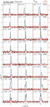 |
Fig. B.14 Same as Fig. B.4, but for secondary filaments converging to F3, F4, F5 and F7. |
| In the text | |
Current usage metrics show cumulative count of Article Views (full-text article views including HTML views, PDF and ePub downloads, according to the available data) and Abstracts Views on Vision4Press platform.
Data correspond to usage on the plateform after 2015. The current usage metrics is available 48-96 hours after online publication and is updated daily on week days.
Initial download of the metrics may take a while.