© ESO 2019

1 Introduction

Both the atomic and the molecular phase of the Galactic interstellar medium (ISM) have been known to be filamentary for a long time. Interstellar filaments were initially detected in dust extinction (e.g., Schneider & Elmegreen 1979; Myers 2009), dust emission (e.g., Abergel et al. 1994), H I (e.g., Joncas et al. 1992; McClure-Griffiths et al. 2006), and CO emission from both diffuse molecular gas (Falgarone et al. 2001; Hily-Blant & Falgarone 2009) and dense star-forming gas (e.g., Bally et al. 1987; Cambrésy 1999). It is only recently, however, that the ubiquity of filamentary structures in the cold ISM and their importance for the star-formation process have been revealed, thanks to the unprecedented quality and sky coverage of Herschel dust continuum images at far-infrared and submillimeter wavelengths. Prominent filamentary structures have been observed with Herschel in both star-forming and non-star-forming low-mass clouds in the solar neighborhood (e.g., André et al. 2010; Men’shchikov et al. 2010), as well as in massive star-forming complexes throughout the Galactic plane at distances from a few kiloparsec up to the central molecular zone (Molinari et al. 2010; Hill et al. 2011; Hennemann et al. 2012; Schneider et al. 2012; Schisano et al. 2014; Wang et al. 2015). Filaments are also striking features in numerical simulations of molecular cloud formation and evolution (e.g., Mac Low & Klessen 2004; Vázquez-Semadeni et al. 2007; Hennebelle et al. 2008; Nakamura & Li 2008), even if the resulting filament properties do not always match the observed ones (e.g., Hennebelle 2013; Federrath 2016; Ntormousi et al. 2016; Smith et al. 2016).

Quite unexpectedly, our early analysis of the radial column density profiles observed with Herschel for 90 filaments in three nearby clouds (IC5146, Aquila, and Polaris) suggested that molecular filaments share a common inner width of about 0.1 pc despite a wide range of central column densities (Arzoumanian et al. 2011). Moreover, the results of the Herschel Gould Belt survey (e.g., André et al. 2010; Könyves et al. 2015; Marsh et al. 2016) indicate that most prestellar cores form in dense, “supercritical” filaments for which the mass per unit length exceeds the critical line mass of nearly isothermal, long cylinders (cf. Inutsuka & Miyama 1997), $M_{\text{line},\text{crit}}=2c_{\text{s}}^2/G~16M_{\odot }/\text{pc}$, where c_s ~ 0.2 km s⁻¹ is the isothermal sound speed for cold molecular gas at T_gas ~ 10 K. Based on Herschel results in nearby clouds, it has also been argued that filaments may help to regulate the star-formation efficiency in the dense molecular gas of galaxies, and may be responsible for a quasi-universal star-formation law in the dense ISM of galaxies (cf. Shimajiri et al. 2017, see also Lada et al. 2012; Toalá et al. 2012). These findings support a paradigm for star formation inwhich the formation and fragmentation of molecular filaments play a central role (cf. André et al. 2014; Inutsuka et al. 2015). To further improve our understanding of the initial conditions and “microphysics” of star formation in the cold ISM of galaxies, characterizing the detailed properties of nearby molecular filaments is of paramount importance.

One of the cornerstones of the proposed filamentary paradigm for solar-type star formation (André et al. 2014) is the existence of a characteristic filament width ~ 0.1 pc suggested by the early analysis of Herschel filament properties by Arzoumanian et al. (2011). Recently, Panopoulou et al. (2017) challenged the conclusion of Arzoumanian et al. (2011). Noting the tension between the presence of a characteristic filament width and the absence of any characteristic scale in the power spectrum of interstellar cloud images (Miville-Deschênes et al. 2010, 2016), they discussed potential biases in measurements of filament widths based on simple Gaussian fitting of the radial column density profiles.

Here, we extend our previous study of the radial density structure and basic properties of molecular filaments to a much broader sample of filaments observed with Herschel in eight nearby clouds, using an improved and more automated method for filament identification, extraction, and characterization. We complement our analysis of the Herschel images with multiple tests performed on synthetic maps to estimate the completeness level of the extracted filament sample and the reliability of the derived filament properties. In particular, we address the concerns raised by Panopoulou et al. (2017) on possible measurement biases. Our results essentially confirm and strengthen our earlier findings on filament properties (e.g., Arzoumanian et al. 2011; Peretto et al. 2012; Palmeirim et al. 2013; Alves de Oliveira et al. 2014; Benedettini et al. 2015; Cox et al. 2016). In a parallel paper (Roy et al. 2018), we also show that the essentially scale-free power spectra of Herschel images are consistent with the presence of a characteristic filament width ~ 0.1 pc and do not invalidate the conclusions drawn from the analysis of filament profiles.

The present paper is organized as follows. Section 2 describes the different steps of the method employed to identify/extract filamentary structures in molecular clouds. Section 3 details the steps followed to measure the properties of the filament sample. Three Appendices (A, B, and C) complement these two sections by summarizing multiple analyses performed on synthetic maps to estimate the completeness limit of the filament sample and the reliability of measuring their properties. Section 4 presents the statistics of the measured filament properties. In Sect. 5, we discuss the implications of our results for our theoretical understanding of filament formation and evolution in the cold ISM, and the link with the star-formation process. Finally, Sect. 6 summarizes our main findings.

2 Identifying filaments in nearby molecular clouds

In this paper, we make use of the optically thin sub-millimeter dust continuum emission imaged with the Herschel Space Observatory(Pilbratt et al. 2010) to study the column density structure of eight nearby molecular clouds (distance <500 pc) observed as part of the Herschel Gould Belt survey (HGBS, André et al. 2010). The clouds analyzed here span a wide range of physical conditions, from active intermediate- or high-mass cluster-forming regions such as Ophiuchus, Aquila, and Orion, to low-mass star-forming regions like the Pipe nebula, Taurus L1405, IC5146, and Musca, to a quiescent, non-star-forming region like the Polaris Flare. Table 1 summarizes the properties of the target clouds and gives the distance, projected size (on the plane of the sky), and mass of each region, along with appropriate references.

To take a census of individual filaments in each of these clouds, the first step is to follow the crests of filamentary structures in the corresponding Herschel column density maps. For this purpose, we used the DisPerSE algorithm which is a powerful tool to trace filament networks (Sousbie 2011). While other methods have recently been developed (e.g., Men’shchikov 2013; Clark et al. 2014; Schisano et al. 2014; Koch & Rosolowsky 2015, and others), we have chosen DisPerSE, which has been successfully used since 2011 (Arzoumanian et al. 2011) to trace the filamentary web of the ISM revealed by Herschel observations of star-formingclouds (e.g., Hill et al. 2011; Peretto et al. 2012; Schneider et al. 2012; Palmeirim et al. 2013), and nonHerschel observations (e.g., Panopoulou et al. 2014; Li et al. 2016), as well as in numerical simulations (e.g., Smith et al. 2016; Federrath 2016).

In the following subsections, we describe our methodology and the successive steps taken to build a filament sample from the Herschel observations of the target clouds.

2.1 Working definition of a filament

We define a molecular filament as any elongated structure detected in a two-dimensional (2D) column density map of a molecular cloud, which has a minimum aspect ratio (AR) and a minimum column density excess over the local background.

The AR of a filamentary structure is defined by $$\text{AR}=l_{\text{fil}}/W_{\text{fil}},$$(1)

where l_fil and W_fil are the length and the width of the structure, respectively. The length l_fil scales with the number of pixels tracing the crest of the structure in the input column density map. An elongated structure that is not entirely straight is longer than a straight one, for the same origin and end points.

The intrinsic column density contrast of a filament is defined as $$C^0=(N_{{\text{H}}_2}{}^{\text{fil}}-N_{{\text{H}}_2}{}^{\text{bg}})/N_{{\text{H}}_2}{}^{\text{bg}}=N_{{\text{H}}_2}{}^0/N_{{\text{H}}_2}{}^{\text{bg}},$$(2)

where $N_{{\text{H}}_2}{}^{\text{fil}}$ and $N_{{\text{H}}_2}{}^{\text{bg}}$ are the column densities observed along the crest of the filament and toward the local background, respectively. The column density amplitude of the filament is $N_{{\text{H}}_2}{}^0=N_{{\text{H}}_2}{}^{\text{fil}}-N_{{\text{H}}_2}{}^{\text{bg}}$. The column densities appearing in Eq. (2) are estimated at each map pixel along the filament crest and then averaged along the crest.

2.2 Tracing networks of filaments with the DisPerSE algorithm

To trace filament networks, we adopted DisPerSE (Sousbie 2011)¹, an algorithm designed to identify persistent topological features such as peaks, voids, and filamentary structures in astrophysical data sets. DisPerSE stands for Discrete Persistent Structures Extractor and was initially developed to analyze large-scale filamentary structures in the galaxy distribution, that is, the cosmic web (Sousbie et al. 2011).

The DisPerSE algorithm traces filaments by connecting critical points (e.g., saddle points and maxima) with integral lines, following the gradient in a map. Critical points are the positions where the gradient of the map is zero. We refer to the unique integral line that joins two connected critical points as an “arc”. The absolute difference between the two map values at a pair of critical points is called the persistence of the pair. In DisPerSE, the concept of persistence is used to select the pairs of critical points that have a persistence, that is, a difference larger than a minimum threshold value: the persistence threshold. This approach selects topological features that are robust with respect to data noise and “background fluctuations”.

In a first step, DisPerSE builds a “skeleton” of crests tracing all of the arcs with a persistence larger than the specified persistence threshold. In a second step, DisPerSE (1) removes the arcs of the skeleton based on a robustness criterion and (2) assembles aligned arcs into longer filaments whenever the relative orientation between two neighboring arcs is smaller than a pre-defined assembly angle. The robustness parameter can be understood as a measure of how much contrast an arc has with respect to the local background. In practice, this parameter is measured by DisPerSE by comparing the mean map value along an arc with the local background values at the scale of the arc. The derived skeleton is then reprojected onto the same grid as the input image, after smoothing the arcs over a given number of pixels. The result of these two steps is a skeleton tracing the crests of the network of filaments in the input map for the specified persistence and robustness thresholds.

The free parameters of the DisPerSE run are thus the following: the persistence threshold (PT), the robustness threshold (RT), the maximum assembly angle (AA) between neighboring connected arcs at the assembling step, and the number of pixels (N_pix) used to smooth the skeleton before reprojection onto the same grid as the input image.

2.3 Using DisPerSE on Herschel column density maps

In the analysis presented in this paper, we used column density maps derived from Herschel imaging data taken as part of the HGBS². The $N_{{\text{H}}_2}$ column density maps of the eight regions discussed here were produced following the same procedure as described in Sect. 4.1 of Könyves et al. (2015) for the Aquila cloud. These $N_{{\text{H}}_2}$ maps were calculated adopting a mean molecular weight per hydrogen molecule ${\text{μ}}_{{\text{H}}_2}=2.8$ (e.g., Kauffmann et al. 2008) and have an estimated accuracy of better than ~ 50% (see Roy et al. 2013, 2014; Könyves et al. 2015). We used both standard $N_{{\text{H}}_2}$ maps at the 36.′′ 3 (half-power beam width – HPBW) resolution of Herschel/SPIRE 500 μm data and “high-resolution” $N_{{\text{H}}_2}$ maps at the 18.′′2 resolution of Herschel/SPIRE 250 μm data. The multi-scale decomposition method used to derive Herschel column density maps at 18.′′ 2 resolution is described in detail in Appendix A of Palmeirim et al. (2013). As examples, Fig. 1 shows the “high-resolution” column density maps of the fields analyzed here in the Orion B and IC5146 clouds (only a portion of the Orion B field is displayed in Fig. 1; see Fig. B.11 for the whole field). The column density maps of the other regions discussed in this paper are shown in Appendix C.

As part of the present study, we ran DisPerSE on column density maps at the standard resolution of 36.′′ 3 and subsequently measured the properties of the extracted filamentary structures in the corresponding high-resolution column density maps (equivalent HPBW = 18.′′ 2). Running DisPerSE on the 36.′′3 resolution column density maps produces skeletons that are smoother (straighter) than when DisPerSE is run on the 18.′′ 2 high resolution maps. In this context, an appropriate choice for the PT to be used when running DisPerSE is on the order of the minimum root mean square (rms_min) level of the “backgroundcloud fluctuations” in the input column density map. An appropriate value for the RT is on the order of the minimum filament $N_{{\text{H}}_2}$ amplitude to be detected in the maps. The robustness threshold is thus linked to the minimum column density contrast of the filaments to be extracted, RT$~\text{}{C}^0{N}_{{\text{H}}_2}{}^{\text{bg}}$ (see Appendix A for details). The filament background column density $N_{{\text{H}}_2}{}^{\text{bg}}$ is a local quantity for each filament and varies through the Herschel column density maps. Ideally, therefore, the RT parameter should be given a local value, varying as a function of position in the input column density map. However, this consideration cannot easily be taken into account with the current version of the DisPerSE code. The RT parameter was therefore chosen to be a scaled version of the minimum background column density value, $N_{{\text{H}}_2}{}^{\text{bg},\text{min}}$, observed in each region. In practice, we derived $N_{{\text{H}}_2}{}^{\text{bg},\text{min}}$ and rms_min using the median and the standard deviation of all values in the first bin of the column density histogram of each field, adopting a bin size of 10²¹ cm⁻² (see Appendix A and Fig. A.1b for details).

As a final post-treatment step (outside DisPerSE), the filament skeletons generated by DisPerSE were “cleaned” by removing features shorter than ten times the HPBW resolution of the input images.

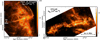Fig. 1 Herschel column density maps of a portion of the analyzed region in Orion B (left panel) and of the entire field analyzed here in IC5146 (right panel), as derived from HGBS data (http://gouldbelt-herschel.cea.fr/archives; cf. André et al. 2010; Arzoumanian et al. 2011; Könyves et al. in prep.). The effective HPBW resolution of these maps is 18.′′ 2. The crests of the filamentary structures traced in the two clouds using DisPerSE as explained in Sect. 2.2 are overlaid as solid curves. The cyan blue curves trace the filament crests of the selected sample, and the dark blue curves trace the crests of additional filaments from the extended sample (cf. Sect. 3.5 and Table 2). The maps of the other fields analyzed in this paper are shown in Appendix C.

2.4 Completeness and reliability of the extracted filament sample

To select optimum parameters for our method of tracing filamentary structures, we performed several tests on synthetic maps including well-defined populations of mock filaments. These tests are described in detail in Appendix A.

The optimum choice of DisPerSE parameters results from a compromise between two conflicting requirements: maximizing the completeness of the extracted filament sample and maximizing the reliability of the sample, that is, minimizing the level of contamination by spurious structures. For a given choice of DisPerSE parameters, the completeness and reliability of the output sample depends on the column density contrast (C⁰) and AR of the filaments to be extracted. To select optimum parameters and estimate the completeness and reliability of our census of filaments in the observed clouds, we therefore applied the method outlined above to synthetic maps and investigated the variations of the fractions of extracted synthetic filaments and spurious structures as a function of PT and RT of the DisPerSE runs on one hand, and the contrast C⁰ and AR of the injected synthetic filaments on the other hand. Another method of choosing appropriate DisPerSE parameters and tracing filament crests has been presented by Green et al. (2017).

The results of our tests, described in Appendix A, indicate that the extracted filament sample is more than 95% complete to filaments with intrinsic contrast C⁰ = 2 for wide ranges of the DisPerSE parameters PT and RT: 0.5 rms_min ≤ PT ≤ 4 rms_min and $0.75N_{{\text{H}}_2}{}^{\text{bg},\text{min}}\le$ RT $\le 2.25N_{{\text{H}}_2}{}^{\text{bg},\text{min}}$, respectively. For synthetic filaments with intrinsic contrast C⁰ = 1, the completeness of the extracted sample is about 95% for RT $\le 1.5N_{{\text{H}}_2}{}^{\text{bg},\text{min}}$ and larger than 80% for RT$=2N_{{\text{H}}_2}{}^{\text{bg},\text{min}}$. The fraction of spurious detections decreases when RT increases. For C⁰ ≥ 1 and RT $\ge 1.5N_{{\text{H}}_2}{}^{\text{bg},\text{min}}$, the fraction of spurious extracted structures is only ~ 5%, but increases rapidly for RT $<1.5N_{{\text{H}}_2}{}^{\text{bg},\text{min}}$.

For a given robustness threshold RT, the fraction of extracted synthetic filaments depends mainly on filament contrast C⁰, and is less affected by the AR of the filaments (see Fig. A.3). For reference, the column density contrast of isothermal model filaments in pressure equilibrium with the ambient cloud is $\langle {\Sigma }_{\text{fil}}\rangle /{\Sigma }_{\text{cloud}}\approx 1.18\times \sqrt{f_{\text{cyl}}/(1-f_{\text{cyl}})}$, where Σ_fil and Σ_cloud are the gas surface densities of the filament and the cloud, respectively, and f_cyl ≡ M_line∕M_line,crit < 1 (cf. Fischera & Martin 2012)³. Therefore, thermally transcritical filaments with M_line,crit∕2≲M_line < M_line,crit (i.e., f_cyl≳0.5) are expected to have column density contrasts C⁰≳1, while thermally supercritical filaments with well-developed power-law density profiles may have C⁰ > > 1.

While the completeness of the extracted filament sample does depend on the adopted robustness threshold, it is not very sensitive to the exact choice of the persistence threshold within a factor of two around the minimum rms value in the map (rms_min). The fraction of extracted synthetic filaments is larger for RT ≤ 1.5–2$N_{{\text{H}}_2}{}^{\text{bg},\text{min}}$, but the fraction of spurious detections also increases. To maximize the fraction of “true” detections while maintaining the fraction of “spurious” detections to a reasonably low level, the best compromise for the choice of the robustness parameter appears to be RT $~\text{}1.5N_{{\text{H}}_2}{}^{\text{bg},\text{min}}$.

In the following analysis, based on the multiple tests of Appendix A, we set PT = rms_min, RT$=1.5N_{{\text{H}}_2}{}^{\text{bg},\text{min}}$, the assembling angle AA to 50°, and the number of pixels of the smoothing kernel N_pix to 2 × HPBW/pix, where pix is the pixel size. Table 2 gives the absolute values of the PT and RT used to trace filamentary structures in each of the eight fields, as well as the number of extracted filaments. The previous discussion and the tests of Appendix A suggest that our census of filamentary structures is more than 95% complete for transcritical and supercritical filaments, with a possible contamination from spurious structures of about ~ 5%. Our sample of subcritical filaments is admittedly less complete and may also contain a larger number of spurious structures.

The filament skeletons⁴ derived as explained above are overlaid as solid curves in Fig. 1 for part of the Orion B field (left panel) and the IC5146 cloud (right panel), respectively (see Figs. B.11–B.14 for the whole Orion B skeleton and the skeletons derived in the other regions).

3 Measurements of filament properties

In this section, we provide details on how we derive radial column density profiles for the extracted filaments and how we estimate properties such as filament width, outer radius, profile shape at large radii, mass per unit length, and so on. The filament properties presented in this paper are derived from measurements performed on Herschel column density maps at 18.′′ 2 resolution.

3.1 Construction of radial profiles for the extracted filaments

To construct radial profiles perpendicular to the long axis of a given filament, we first determine the normal direction to the filament at each point along its crest. To do so, we compute the Hessian matrix H of second-order partial derivatives for all pixels in the corresponding “high-resolution” column density map. The angle α between the x-axis of the Cartesian coordinate system and the local tangential direction to the filament crest is given by: $$\alpha =\frac{1}{2}\arctan \left(\frac{2H_{xy}}{H_{x^2}-H_{y^2}}\right),$$(3)

where the x and y axes are the horizontal and vertical axes of the column density map in Cartesian coordinates, and $H_{x^2}={\partial }^2{N}_{{\text{H}}_2}/\partial x^2$, $H_{y^2}={\partial }^2{N}_{{\text{H}}_2}/\partial y^2$ and $H_{xy}=H_{yx}={\partial }^2{N}_{{\text{H}}_2}/\partial x\partial y$. The angle α + 90° then gives the normal direction to the filament crest at each position (see also Arzoumanian 2012). From the 2 × 2 Hessian matrix, the minimum curvature of the column density field can also be estimated at each point (as the smaller of the two eigenvalues of the matrix), which may then be used to enhance the contrast of filamentary structures in the map. Indeed, a filament is an elongated structure which corresponds to a relatively small curvature of the column density field along its main axis, and a significantly stronger curvature along its short axis, that is, the normal direction to the filament crest. Based on this idea, the Hessian matrix has been used to identify filaments in Herschel and Planck maps (Schisano et al. 2014; Planck Collaboration Int. XXXII 2016). Here, we only use the Hessian matrix to calculate the normal direction to the filament crest, using Eq. (3) on the original $N_{{\text{H}}_2}$ map.

Using the above approach, we thus construct radial profiles at each pixel position along the filament crest in the high-resolution column density map. We then build the median radial column density profile of the filament by computing the median of all radial cuts along the crest. We also derive a set of spatially independent radial profiles for the filament by dividing the crest into consecutive segments of 2 × HPBW length and averaging the radial cuts obtained in each segment of adjacent pixels along the filament crest. As mentioned in Sect. 1, prestellar and protostellar cores are observed along supercritical filaments. The presence of these dense cores may affect estimates of the filament properties locally and should ideally be removed. However, since cores contribute only a small fraction of the mass of dense filaments, typically 15% on average (e.g., Könyves et al. 2015), they are not expected to significantly alter the median profile and median properties of a filament. For simplicity, in this paper, we thus present results derived from an analysis of original $N_{{\text{H}}_2}$ maps without subtracting dense cores.

Figure 2 shows two examples of median radial column density profiles, obtained for a supercriticalfilament in Ophiuchus and a subcritical filament in Taurus. The local dispersion of the radial $N_{{\text{H}}_2}$ profiles (shown in yellow) is estimated as the median absolute deviation $\text{mad}(r)=\text{median}[|N_{{\text{H}}_2}{}^{\text{pix}}(r)-\text{median}(N_{{\text{H}}_2}(r))|]$, where $N_{{\text{H}}_2}{}^{\text{pix}}(r)$ is the value of the $N_{{\text{H}}_2}(r)$ radial profile at each pixel position along the filament crest. Radial dust temperature profiles can be constructed in a similar way from the line-of-sight dust temperature maps derived from Herschel data at 36.′′ 3 resolution (cf. Könyves et al. 2015).

In the following subsections, we describe how filament properties can be derived from the radial profiles. All of the properties discussed below were first measured independently on either side of the filament crest. The values corresponding to the two sides were then averaged.

3.2 Estimating the local background and outer boundary of each filament

Molecular filaments are not isolated structures but are embedded in parent interstellar clouds which often exhibit complex, multi-scale internal structure. To measure the properties of an individual filament, one should first estimate its outer boundaries and characterize the local background, that is, the emission properties of the parent cloud in the immediate vicinity of the filament. Especially in the case of a low-contrast filament, an accurate determination of the local background is key for deriving intrinsic filament properties but this is not straightforward. Even the B211/B213 filament in Taurus, which has a very clean and very symmetric radial $N_{{\text{H}}_2}$ profile, exhibits some differences in background properties on either side of its long axis (Palmeirim et al. 2013). Here, we therefore perform separate measurements on either side of the filament axes.

At each point s along the crest, the outer radius R_out (s) of a filament may be defined as the radial distance from the filament axis at which the amplitude $N_{{\text{H}}_2}{}^0=N_{{\text{H}}_2}{}^{\text{fil}}-N_{{\text{H}}_2}{}^{\text{bg}}$ of the radial column density profile becomes negligible compared to the column density $N_{{\text{H}}_2}{}^{\text{bg}}$ of the background cloud (without beam deconvolution). In practice, R_out(s) can be estimated from the observed radial column density profile as the closest point to the filament crest for which the logarithmic slope of the profile $\text{d\hspace{0.17em}ln}{N}_{{\text{H}}_2}/\text{d\hspace{0.17em}ln}r$, smoothed over 3 × HPBW, is consistent with zero (see Fig. 2). Strictly speaking, two outer radii $R_{\text{out}}^{\pm }(s)$ are defined at each point s on either side of the filament axis. The column density $N_{{\text{H}}_2}{}^{\text{bg}\pm }(s)$ of the background cloud on either side of the filament crest is assumed to be constant: $N_{{\text{H}}_2}{}^{\text{bg}\pm }(s)=N_{{\text{H}}_2}(r=R_{\text{out}}^{\pm }$; see Fig. 2).

Once $R_{\text{out}}^{\pm }$, $N_{{\text{H}}_2}{}^{\text{bg}\pm }$, and $N_{{\text{H}}_2}{}^0$ have been estimated, the half-power radius hr^± of the filament (on either side of the main axis) may be derived without any fitting of the radial profile, as the radial distance from the filament crest where the background-subtracted amplitude of the observed profile is half of the value on the crest, that is, 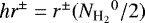$h{r}^{\pm }=r^{\pm }(N_{{\text{H}}_2}{}^0/2)$. The quantity hd ≡ 2hr or hr⁺ + hr⁻ provides a first estimate of the filament width (see Fig. 2). We deconvolve the measured 2hr width from the equivalent HPBW = 18.′′2 beam of the high-resolution column density map using the following approximation: $h{d}_{\text{dec}}=\sqrt{{(2hr)}^2-HPB{W}^2}$, where hd_dec is the estimated half-power diameter after deconvolution.

To summarize, estimates of R_out(s), $N_{{\text{H}}_2}{}^{\text{bg}}(s)$, and hd(s) are obtained at each point along, and on either side of, the crest of each filament. In practice, the quantities used in Sects. 4 and 5 below correspond to the medians of the R_out(s), $N_{{\text{H}}_2}{}^{\text{bg}}(s)$, and hd(s) values derived from the set of spatially independent profiles for each filament. The profiles shown in Figs. 2 and 3 correspond to the median radial column density profiles of four filaments taken as examples.

Fig. 2 Fromleft to right columns: median radial column density profile observed on either side of the filament axis in lin-lin format (panels A), median radial column density profile on the left-hand side of the crest (i.e., r < 0 in A1 andA2) in log-log format (panels B), and panels C: logarithmic slope of the column density profile ($\text{d\hspace{0.17em}ln}{N}_{{\text{H}}_2}/\text{d\hspace{0.17em}ln}r$) as a function of radius from the central crest, for a filament in the Ophiuchus cloud (top three panels, A1, B1, C1) and a filament in the Taurus cloud (bottom three panels, A2, B2, C2). In Cols. A and B, the yellow area/error bars correspond to the median absolute deviation (mad(r)) of the distributions of independent cuts taken perpendicular to the filament crest (see Sect. 3.1). In Col. A, the outer radii $R_{\text{out}}^{\pm }$ (vertical dotted red line) and the background column densities $N_{{\text{H}}_2}{}^{\text{bg}}\pm$ (horizontal red line) are marked. In Col. B, the observational beam of 18.2′′ (blue curve), the outer radius $R_{\text{out}}^{-}$ (vertical dotted red line), the background column density $N_{{\text{H}}_2}{}^{\text{bg}}-$ (horizontal red line), and the half power radius hr− (vertical dotted yellow line) are shown. As explained in Sect. 3.2, the values of $R_{\text{out}}^{\pm }$, $N_{{\text{H}}_2}{}^{\text{bg}}\pm$, and hr± were derived from the data independently on either side of the filament crest, using the logarithmic slope plot Col. C smoothed over 3 × HPBW. In Col. C, the black solid curve represents the logarithmic slope profile at the original resolution, while the blue symbols show the logarithmic slope profile smoothed over 3 × HPBW; the red dotted vertical line marks the derived outer radius $R_{\text{out}}^{-}$, and the black dotted horizontal line marks a zero slope (flat column density profile).

3.3 Fitting the filament radial profiles

The radial column density profiles of each filament were fitted with both Gaussian and Plummer-like functions.

For each filament, separate fits were derived on either side of the main axis using (1) the median radial column density profiles and (2) the set of spatially independent radial profiles constructed along the filament crest. In the latter case, median parameter values were calculated from the distribution of fitting parameters obtained along the crest. In both cases, the parameters of the fits found on either side were also averaged. This approach resulted in two values for each fitting parameter, one derived from the median radial profiles and the other corresponding to the median parameter value along the filament crest.

In the next two subsections, we describe the Gaussian and Plummer fitting procedures, respectively. Section 3.3.3 gives details on the link between the filament widths derived from the two fitting methods. The reliability of the derived parameter values is discussed in Sect. 3.5.

3.3.1 Gaussian function fitting

Each $N_{{\text{H}}_2}(r)$ profile was fitted for r ≤ 1.5 hr with a one-dimensional Gaussian function of the form, $$N_{{\text{H}}_2}{}^{\text{G}}(r)=N_{{\text{H}}_2}{}^{0,\text{G}}\exp \left[-4\ln 2{(r/FWHM)}^2\right]+N_{{\text{H}}_2}{}^{\text{bg},\text{G}},$$(4)

where the column density amplitude, $N_{{\text{H}}_2}{}^{0,\text{G}}$, the FWHM width, and the (uniform) background column density $N_{{\text{H}}_2}{}^{\text{bg},\text{G}}$ estimated from the observed column density at r = 1.5 hr, $N_{{\text{H}}_2}(r=1.5hr)$, are the three free parameters of the fit. The free parameters of the fit were bounded as follows: $0.7N_{{\text{H}}_2}{}^0\le N_{{\text{H}}_2}{}^{0,\text{G}}\le 1.3N_{{\text{H}}_2}{}^0$, $0.7N_{{\text{H}}_2}(r=1.5hr)\le N_{{\text{H}}_2}{}^{\text{bg},\text{G}}\le 1.3N_{{\text{H}}_2}(r=1.5hr)$, and 0 < FWHM ≤ R_out. Each fitted data point was weighted by its median absolute deviation (mad; see yellow error bars in Fig. 2 – see also Sect. 3.1). The fitted FWHM width was then deconvolved from the observational HPBW beam as $FWH{M}_{\text{dec}}=\sqrt{FWH{M}^2-HPB{W}^2}$, where HPBW = 18.′′2 is the effective resolution of the corresponding high-resolution column density map.

3.3.2 Plummer-like function fitting

The radial column density profiles of observed filaments often exhibit power-law wings which cannot be well represented by a Gaussian function and are better reproduced by a Plummer function (see Fig. 3 and e.g., Arzoumanian et al. 2011; Palmeirim et al. 2013; André et al. 2016; Cox et al. 2016). Using a Plummer-like function (Eq. (5)), one can in principle reproduce the behavior of the radial column density distribution for both r ≤ R_flat and r ≫R_flat, which is not possible with a Gaussian fit.Each median $N_{{\text{H}}_2}(r)$ profile was therefore fitted with the following function. $$N_{{\text{H}}_2}{}^{\text{Pl}}(r)=N_{{\text{H}}_2}{}^{0,\text{Pl}}/{\left[1+{\left(r/R_{\text{flat}}\right)}^2\right]}^{\frac{p-1}{2}}+N_{{\text{H}}_2}{}^{\text{bg},\text{Pl}},$$(5)

where R_flat is the radius of a flat inner region with approximately constant (column) density, p is the power-law exponent of the corresponding density profile for r ≫ R_flat, $N_{{\text{H}}_2}{}^{0,\text{Pl}}$ is the central column density of the Plummer-like model filament, and $N_{{\text{H}}_2}{}^{\text{bg},\text{Pl}}$ is the background column density (here assumed to be independent of r). The fitting was performed up to r = R_out. The free parameters of the fit were $N_{{\text{H}}_2}{}^{0,\text{Pl}}$, $N_{{\text{H}}_2}{}^{\text{bg},\text{Pl}}$, R_flat, and p. The free parameters were bounded as follows: $0.7N_{{\text{H}}_2}{}^0\le N_{{\text{H}}_2}{}^{0,\text{Pl}}\le 1.3N_{{\text{H}}_2}{}^0$, $0.7N_{{\text{H}}_2}(r=R_{\text{out}})\le N_{{\text{H}}_2}{}^{\text{bg},\text{Pl}}\le 1.3N_{{\text{H}}_2}(r=R_{\text{out}})$, 0 < R_flat ≤ R_out, and 1.2 ≤ p ≤ 3.5. The Plummer-like model function described by Eq. (5) was first convolved with the 18.′′ 2 Gaussian beam of the corresponding column density map prior to comparison with the observed profile.

Recovering the intrinsic R_flat value when fitting R_flat and p simultaneously is difficult in the case of low-contrast filaments due to a partial degeneracy between the two parameters whose errors are anti-correlated (as discussed by, e.g., Malinen et al. 2012; Juvela et al. 2012; Smith et al. 2014). The results are nevertheless satisfactory for high-contrast filaments C⁰ ≥ 1, such as the Taurus B211/B213 filament (Palmeirim et al. 2013). We thus derived two estimates of R_flat: R_flat(1) from fit 1, obtained by fixing the power-law exponent to p = 2 and leaving R_flat as a free parameter, and R_flat(2) from fit 2, leaving both R_flat and p as free parameters.

As an illustration, Fig. 3 shows the median radial $N_{{\text{H}}_2}$ profiles of four filaments observed in different regions along with the corresponding best Gaussian and Plummer fits.

3.3.3 Filament width

For each radial column density profile constructed from Herschel data, we derived three estimates of the corresponding filament width: a deconvolved half-power diameter hd_dec (from the deconvolved 2hr value) without any fitting of the profile, a deconvolved FWHM_dec width resulting from a Gaussian fit for r ≤ 1.5 hr, and a (deconvolved) flat inner diameter D_flat = 2R_flat resulting from a Plummer-like function fit for r ≤ R_out. These three different estimates of the inner width of each filament are discussed further in Sect. 4.

We stress that, in the presence of power-law wings, both the measured half-power diameters hd and the results of Gaussian fits must be interpreted with caution. In particular, as pointed out by, for example, Smith et al. (2014); Panopoulou et al. (2017), the FWHM widths derived from Gaussian fitting are affected by the range of radii used in the fits. Figure 4 illustrates the link between the half-power diameter hd, the FWHM width derived from a Gaussian fit, and the intrinsic flat inner diameter 2 R_flat of a Plummer-like model profile with p = 2, for several fitting ranges. In this case, $hd=1.6(2R_{\text{flat}}^{p=2})$ and $FWHM=1.1(2R_{\text{flat}}^{p=2})$ when the profile is fitted for radii 0 ≤ r ≤ 1.5 hr. The relation between FWHM and $2R_{\text{flat}}^{p=2}$ changes by ± 20% when the fitting range varies between hr and 3hr. For Plummer-like model profiles with p = 1.5, p = 2.5, and p = 3, $FWHM=1.6(2R_{\text{flat}}^{p=1.5})$, $FWHM=0.9(2R_{\text{flat}}^{p=2.5})$, and $FWHM=0.8(2R_{\text{flat}}^{p=3})$, when the profile is fitted for r ≤ 1.5 hr, with uncertainties of ± 40%, ± 11%, and ± 8% respectively, when the fitting range varies between hr and 3hr.

3.4 Filament mass per unit length

As introduced in Sect. 1, the mass per unit length (M_line) of a filament is a very important parameter which, by comparison with the critical line mass M_line,crit, may be used to diagnose whether the filament is unstable to gravitational collapse as a cylindrical structure.

When the filament profile is well approximated by a Gaussian function, M_line can be estimated by multiplying the central surface density of the filament by the FWHM width (cf. Appendix A of André et al. 2010). When the $N_{{\text{H}}_2}$ profile is not Gaussian-like and/or includes a significant power-law wing, however, the latter approximation of M_line may underestimate the true M_line. To investigate the relevance of the shape of the radial column density profile for estimating the filament M_line, we derived and compared three (partly independent) estimates of M_line, making use of our detailed analysis of the radial profiles:

• $M_{\text{line}}^{\text{w}}={\Sigma }_{\text{fil}}^0\times W_{\text{fil}}$, where ${\Sigma }_{\text{fil}}^0={\mu }_{{\text{H}}_2}{m}_{\text{H}}{N}_{{\text{H}}_2}{}^0$ is the central gas surface density of the filament, W_fil = 2hr is the filament width estimated without any fitting, ${\text{μ}}_{{\text{H}}_2}$ the mean molecular weight per hydrogen molecule, and m_H the mass of a hydrogen atom.

• $M_{\text{line}}{}^{\text{int}}=2{\displaystyle {\int }_0^{R_{\text{out}}}}{\mu }_{{\text{H}}_{\text{2}}}{m}_{\text{H}}(N_{{\text{H}}_2}(r)-N_{{\text{H}}_2}{}^{\text{bg}})\text{\hspace{0.17em}d}r$, integrating the column density profile over radius up to R_out, after background subtraction.

• M_fil∕l_fil, where M_fil is the total mass of the filament calculated by summing the background-subtracted column density over the pixels contained in the area around the filament crest bounded by the outer radius values R_out measured along the filament crest (see Sect. 3.2), and l_fil is the total length of the filament.

3.5 Reliability of derived filament properties

Before discussing the statistical properties of the extracted filament sample in Sect. 4 below, the reliability of our method of measuring filament properties must be assessed. To this end, we tested the measurement procedures described in the previous subsections using synthetic maps. These tests are described in detail in Appendices B.1 and B.2.

Briefly, we distributed several sets of synthetic filaments with both Gaussian and Plummer density profiles within a realistic “background” column density map. The synthetic filaments were given uniform, Gaussian, or power-law distributions of input properties (FWHM, D_flat, p) along their crests. The various measurements/fitting steps described in Sects. 3.1–3.4 above were then applied to the synthetic maps. For synthetic filaments with Gaussian profiles, the measured hd = 2hr values, derived without any fitting, reproduce the input FWHM widths. Moreover, the resulting distributions of FWHM widths estimated from Gaussian fitting are in excellent agreement with the input distributions of FWHM values for any fitting range between [0,1.5hr] and [0,3hr] (Appendix B.1). In particular, a peaked distribution of measured FWHM widths is recovered solely when the input synthetic filaments have a constant width along their crests or a narrow Gaussian distribution around the mean width value (see Figs. B.2A and B.3). In addition the distribution of measured FWHM widths is flat or has a power-law distribution down to the resolution limit of the column density map when the input filaments have a flat or power-law distribution of widths (constant along their crest), respectively, (see Figs. B.2B,C). The values of the input filament lengths, column density contrasts C⁰, and masses per unit length M_line, are also well recovered.

In the case of synthetic filaments with Plummer-like profiles, the median value of the FWHM widths derived from Gaussian fitting is significantly affected by the fitting range (see Fig. 4, and also Smith et al. 2014; Panopoulou et al. 2017). However, for a given fitting range (e.g., for 0 ≤ r ≤ 1.5hr), a peaked distribution of measured FWHM values is obtained only when the input R_flat values are the same for all mock filaments, while a power-law distribution down to the resolution limit of the synthetic map is recovered when the input mock filaments have a power-law distribution of R_flat values (see Fig. B.4). Moreover, both the R_flat and the p parameters of the synthetic Plummer filaments are reasonably well recovered by our Plummer-fitting method, independently of the input distributions of R_flat values (uniform, flat, or power law) and p values (uniform, flat, or Gaussian), and whether the input R_flat values were constant along the filament crests (see Figs. B.4–B.9) or not (see Fig. B.10). The measurements however become increasingly more uncertain for lower contrast (C < 1) filaments, as can be seen for instance by comparison of Fig. B.6 with Fig. B.5.

For Plummer-like input filament profiles, both the FWHM widths derived from Gaussian fitting and the hd values (derived without any fitting) are affected by changes in the input power-law slope p. The derived FWHM widths are closest to the input D_flat = 2R_flat values when the fitting range is 0 ≤ r ≤ 1.5hr. If this fitting range is adopted, the derived FWHM widths provide estimates of the D_flat diameters that are accurate to better than ~ 50% for high-contrast (C⁰ > 1) filaments when 1.5 < p < 3. The uncertainties in the derived FWHM widths are also smaller than those in the derived hd values.

Based on the reliability tests and uncertainty assessments of Appendix B, we present and discuss the statistical distributions of our three estimates of the filament inner width (hd_dec, FWHM_dec, and D_flat) in Sect. 4 below. We adopt the FWHM_dec estimates as our reference measurements of the inner width, giving satisfactory results for both Gaussian-like filaments and Plummer-like filaments. We stress, however, that the D_flat estimates are more appropriate and more accurate in the case of high-contrast, dense filaments with power-law wings.

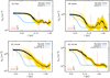Fig. 3 Radial column density profiles (in log–log format) observed perpendicular to, and averaged along, the crestsof four filaments in four different clouds. The cloud name is indicated at the top left of each panel. The blue and red dashed curves show the best Gaussian and Plummer fits, respectively (see Sect. 3.3). Panels A and B: observed profiles are Gaussian-like and the derived (hddec, FWHMdec) widths are (0.11 pc, 0.12 pc) and (0.09 pc, 0.09 pc), respectively. Panels C and D: inner parts of the profiles are well reproduced by Gaussian functions, but the outer parts show power-law wings, which are much better fitted with Plummer functions. The derived (hddec, FWHMdec, Dflat, and p) parametes are (0.14 pc, 0.10 pc, 0.09 pc, 2.2) and (0.16 pc, 0.11 pc, 0.08 pc, 2.2), for panels C and D, respectively. On each plot, the blue solid curve represents the effective beam resolution of the column density map (18.2′′). The half-power radius hr, outer radius Rout, and background column density (bg), are also indicated (see legend on the bottom left of the panels and Sect. 3.2). The black thick section of each profile indicates the fitting range of the Gaussian fits (i.e., r ≤ 1.5hr). The Plummer fits were performed for r ≤ Rout. The yellow area/error bars correspond to the median absolute deviations [mad(r)] of the distribution of independent cuts taken perpendicular to the filament crest (see Sect. 3.1).

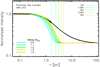Fig. 4 Gaussian fits (colored curves) to the radial column density profile $N_{{\text{H}}_2}(r)$ of a model filament with a Plummer profile (black curve) described by Eq. (5) with p = 2, $N_{{\text{H}}_2}{}^{\text{bg}}=0.2N_{{\text{H}}_2}{}^0$, and Rflat = 1 pc, for five choices of the fitting range: r ∈ [0, hr], [0, 1.5hr], [0, 2hr], [0, 2.5hr], and [0, 3hr] (see vertical dotted lines and color coding at the top right of the plot), where hr = 1.6 Rflat. The FWHM width values obtained from the Gaussian fits are given in units of Dflat = 2 Rflat at the bottom left of the plot.

3.6 Filament samples

Table 2 gives the absolute values of the persistence and robustness thresholds used to trace filamentary structures in each of the eight target fields, for PT = rms_min and RT$=1.5N_{{\text{H}}_2}{}^{\text{bg},\text{min}}$. The entire set of filaments resulting from the extraction method described in Sect. 2 is referred to as the “total filament sample” and comprises a total number of $N_{\text{tot}}^{\text{fil}}=1310$ filaments. After measuring the properties of each of these 1310 filamentary structures, we selected a subset of more robust filaments satisfying the following two additional conditions: $$\text{AR}>3\text{\hspace{0.17em}\hspace{0.17em}and\hspace{0.17em}\hspace{0.17em}}{C}^0>0.3,$$

where AR = l_fil∕W_fil with W_fil = FWHM, and $C^0=N_{{\text{H}}_2}{}^0/N_{{\text{H}}_2}{}^{\text{bg}}$. This selection discards a fraction of filamentary structures which may be strongly contaminated by spurious features (see Appendix A and Fig. A.3) or may be associated with elongated cores rather than filaments (for AR ≲ 3). The number of filaments in this selected sample is $N_{\text{select}}^{\text{fil}}=599$.

4 Statistical properties of the extracted filament sample

This section presents the statistical properties of the filament sample extracted as explained in Sect. 2 in the eight fields of Table 1, all imaged with Herschel as part of the HGBS. In all of the following plots, the filaments detected in each region are represented by specific colored dots (cf. Table 1 for the color coding). In Sect. 4.1, we first discuss the distributions of median properties resulting from “averaging” about 10 – 30 independent measurements along and on either side of each filament crest. Properties such as filament column density, dust temperature, width, outer radius, length, mass per unit length, and column density contrast, estimated using the measurement steps described in Sect. 3 and averaged along the filament crests, are discussed. We also investigate possible correlations between these various filament-averaged properties. Tables 3–5 summarize the global properties of the subsets of filaments identified in each field. In particular, the mean value and the standard deviation of each fitted parameter are provided in Table 3 (for Gaussian fits) and Table 4 (for Plummer fits) for the eight fields. The median value of each parameter and the equivalent standard deviation estimated from the interquartile range (IQR) assuming Gaussian statistics are also provided. For a Gaussian distribution, the standard deviation σ corresponds to the IQR divided by a factor 1.349. Finally, in Sect. 4.2, we discuss the filament properties derived prior to any averaging along the filament crests.

4.1 Statistical results on filament-averaged properties

The extended and selected samples comprise 1310 and 599 filaments, respectively (see Figs. 5 and 6). Both samples span a broad range of central column densities $N_{{\text{H}}_2}{}^0$, from a few 10²⁰ cm⁻² for the faintest filaments up to a few 10²² cm⁻² for the densest filaments (Fig. 5). Likewise, the extracted filaments span a wide range in mass per unit length from M_line < 1 M_⊙pc⁻¹ for the most thermally subcritical up to M_line ≳ 100 M_⊙pc⁻¹ for the mostthermally supercritical filaments.

The line-of-sight integrated dust temperatures measured toward the filament crests ($T_{\text{dust}}^{\text{crest}}$) are found to be typically ~15 K with a dispersion of about 3 K. The dust temperature along the filament crests, $T_{\text{dust}}^{\text{crest}}$, is generally found to be colder than the temperature of the surrounding ambient cloud, $T_{\text{dust}}^{\text{bg}}$ (see Fig. 6B). This behavior is consistent with the description of a molecular filament as a 3D cylindrical structure, where the increase in column density corresponds to an increase in density (cf. Li & Goldsmith 2012; Palmeirim et al. 2013). In the absence of luminous embedded protostars, the dust in the filament interior is more shielded from the ambient interstellar radiation field than the dust in the filament envelope and is therefore colder.

The ranges of background column densities $N_{{\text{H}}_2}{}^{\text{bg}}$ spanned by the filaments in the entire and selected samples can be seen in Figs. 5B and 6C, respectively. Even within the same molecular cloud, the background column density can vary significantly, that is, by at least an order of magnitude in most regions. There is also a significant correlation between $N_{{\text{H}}_2}{}^0$ and $N_{{\text{H}}_2}{}^{\text{bg}}$ (Fig. 6C). These results suggest that environmental properties, such as ambient gas pressure, may change significantly from one filament to the other, even within the same cloud, possibly affecting their evolution. In each cloud, the observed filaments span a wide range in column density contrast C⁰ regardless of their $N_{{\text{H}}_2}{}^{\text{bg}}$ (Fig. 5B).

Figure 5D shows a plot of filament outer diameter 2R_out as a function of filament intrinsic column density contrast C⁰. High-contrast filaments tend to have larger outer diameters owing to more developed power-law wings. We see similar correlations between 2R_out and M_line or $N_{{\text{H}}_2}{}^0$ (not shown here). However, there is no correlation between the length l_fil or the inner width W_fil and either the central column density $N_{{\text{H}}_2}{}^0$ or the mass per unit length M_line. While the filament lengths span a wide range from ≳ 0.1 pc up to a few parsecs, the deconvolved half-power widths W_fil = hd_dec have a low dispersion around a median value of 0.1 pc (see Fig. 5C). Accordingly, the ARs of the filaments in the selected sample span a wide range from a minimum of 3 (defined by one of our selection criteria) up to ~ 30 for the longest filaments (see Fig. 6A). About 59 and 14% of the filaments have AR > 5 and AR > 10, respectively. While the filaments detected in the HGBS images are typically parsec-scale structures, Herschel observations of more massive star-forming regions at approximately kiloparsec distances have revealed longer filaments in the Galactic plane (e.g., Molinari et al. 2010; Schisano et al. 2014).

The deconvolved FWHM widths of the 599 filaments in our selected sample, as measured from Gaussian fits to their radial column density profiles, have a narrow distribution centered around a median value of 0.09 pc, with an equivalent standard deviation of 0.05 pc (scaled from a measured IQR of 0.07 pc – see Fig. 7 and Table 3). The deconvolved hd values also have a narrow distribution about a median value of 0.11 pc and an equivalent standard deviation of 0.05 pc (Table 3). The same filaments span more than two orders of magnitude in central column density (cf. Fig. 8), implying a spread of two orders of magnitude in the distribution of central Jeans lengths [${\lambda }_{\text{J}}\left(r=0\right)=c_{\text{s}}^2/\left(G{\Sigma }_{r=0}\right)$], which is much broader than the observed spread in the distribution of filament widths. The horizontal dotted lines in Fig. 8 show the spatial resolution limits of the column density maps used to construct the filamentprofiles. The measured filament widths are always significantly above the corresponding resolution limit. Moreover, we stress that only the physical widths of the filaments (in pc) show a narrow distribution (cf. Fig. 7), while the angular widths (in arcsec) vary as a function of the parent cloud distances (see Table 3 and also Table 2 in Arzoumanian et al. 2011). This strongly suggests that the ~ 0.1 pc inner width is an intrinsic physical property of the observed filaments and is not affected by the finite resolution of the Herschel data. Our earlier result on the existence of a characteristic filament width (for 90 filaments) in three molecular clouds, IC5146, Aquila and Polaris (Arzoumanian et al. 2011), has therefore been generalized to a much larger filament sample and five additional clouds.

Our estimates of the physical filament width are somewhat sensitive to uncertainties in cloud distances (see, e.g., discussion in Arzoumanian et al. 2011). The median and equivalent standard deviation values quoted above for the distribution of FWHM_dec widths (0.09 ± 0.05 pc) were obtained for the default distances adopted for each region as listed in Table 1. Assuming alternate distances for the studied clouds, namely 950 pc for IC5146 (Harvey et al. 2008), 500 pc for Orion B (Schlafly et al. 2015), 400 pc for Aquila (Bontemps et al. 2010; Ortiz-León et al. 2017), 400 pc for Polaris (Schlafly et al. 2014), and the same distances as the default values for Musca (200 pc), Taurus, and Ophiuchus (140 pc) would lead to a median FWHM_dec value and equivalent standard deviation of 0.15 ± 0.07 pc. While the distribution of filament inner widths is somewhat broader with the alternate cloud distances, the median filament width is only 50% larger than, and remains consistent with, that derived assuming the default distances of Table 1.

Figure 9 presents the distributions of flat inner diameters D_flat = 2 R_flat and power-law indices p derived from Plummer fits to the median column density profiles of the filaments with contrasts C⁰ > 0.3 (solid line histogram) and C⁰ > 1 (dashed line histogram). These plots show that the distribution of D_flat diameters peaks at a median value of about 0.10 pc, with an equivalent standard deviation of 0.08 pc (for C⁰ > 1, see Table 4), which is fully consistent with the FWHM widths derived from Gaussian fits to the inner part of the observed radial profiles (see, e.g., Fig. 7). The distributions of median D_flat widths exhibit, however, larger dispersions than the distribution of median FWHM_dec widths, especially for filaments with C⁰ < 1. This larger dispersion may result from (1) larger measurement uncertainties using the Plummer-like function fitting method and (2) less well defined power-law profiles and outer radii for low-contrast filaments (see tests presented in Appendix B.2). The radial column density profiles of the selected filaments, especially those with column density contrasts C⁰ > 1, tend to show a power-law behavior at r > >hr with an exponent p ≈ 2 (see Figs. 3 and 9, Table 4, and also Arzoumanian et al. 2011; Hill et al. 2012; Palmeirim et al. 2013; André et al. 2016, and others).

The presence of power-law wings with p ~ 2 in the radial column density profiles of many molecular filaments implies that mass per unit length estimates may dependon the outer boundary of the filaments. Interestingly, the radius of this outer boundary, R_out, is observed to increase with the column density contrast (Fig. 5D), central column density, or M_line of the filaments. Such a behavior is indeed expected for a Plummer-like column density profile with fixed p and R_flat, and increasing central column density. For a Gaussian-like radial $N_{{\text{H}}_2}$ profile, the mass per unit length is $M_{\text{line}}{}^{\text{w}}~{\mu }_{{\text{H}}_2}{m}_{\text{H}}{N}_{{\text{H}}_2}{}^0\times W_{\text{fil}}$. For filaments with significant power-law wings at r > > W_fil∕2, however, a non-negligible fraction of the total mass may lie within the non-Gaussian wings (see also Rivera-Ingraham et al. 2016, 2017). This additional mass is taken into account when deriving $M_{\text{line}}{}^{\text{int}}$ by integrating the $N_{{\text{H}}_2}$ profile over radii up to R_out (see Sect. 3.4).

Figure 10 shows correlations between the mass per unit length (derived in three different ways) and the central columndensity of the observed filaments. The correlation between the two estimates of the mass per unit length shows that $M_{\text{line}}{}^{\text{int}}~1.3M_{\text{line}}{}^{\text{w}}$ on average (cf Fig. 10B), suggesting that most filaments have non-Gaussian $N_{{\text{H}}_2}$ profiles, which typically contribute 30% of their total mass on average. Figure 10A shows a very good correlation between $M_{\text{line}}{}^{\text{int}}$ and $N_{{\text{H}}_2}{}^0$. The correlation between these two (partly independent) quantities is consistent with the presence of a common width shared by all filaments of the selected sample. The $M_{\text{line}}{}^{\text{int}}$ estimate is also well correlated with another estimate of the mass per unit length derived as M_fil∕l_fil (see Sect. 3.4). In addition, a good correlation is observed between $M_{\text{line}}{}^{\text{int}}$ and background column density $N_{{\text{H}}_2}{}^{\text{bg}}$ (cf., Sect. 5).

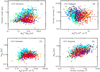Fig. 5 Plots of estimated length lfil against massper unit length $M_{\text{line}}{}^{\text{int}}$ (panel A), column density contrast C0 against background column density $N_{{\text{H}}_2}{}^{\text{bg}}$ (panel B), deconvolved half-power diameter hddec against $N_{{\text{H}}_2}{}^0$ (panel C), and outer diameter (2Rout) against C0, for the entire sample of 1310 extracted filaments (panel D). Panel B: horizontal line corresponds to C0 = 0.3, the minimum contrast imposed as a selection criterion in Sect. 3.5. Panel c: distribution of measured hddec values has a mean of 0.11 pc, a standard deviation of 0.06 pc, a median of 0.10 pc, and an interquartile range of 0.08 pc.

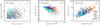Fig. 6 Panel A: aspect ratio (AR) against intrinsic contrast (C0) for the selected sample of 599 filaments with AR > 3 and C0 > 0.3 (see Sect. 3.5). Panel B: median dust temperature difference $T_{\text{dust}}^{\text{crest}}-T_{\text{dust}}^{\text{bg}}$ against $N_{{\text{H}}_2}{}^0$, for the selected sample of 599 filaments. $T_{\text{dust}}^{\text{crest}}$ and $T_{\text{dust}}^{\text{bg}}$ are the line-of-sight dust temperatures averaged along the filament crest and the background, respectively. The horizontal line corresponds to $T_{\text{dust}}^{\text{crest}}=T_{\text{dust}}^{\text{bg}}$. Panel C: filament $N_{{\text{H}}_2}{}^0$ against background column density $N_{{\text{H}}_2}{}^{\text{bg}}$, for the selected sample of 599 filaments. The solid straight line shows the best-fit linear relation $N_{{\text{H}}_2}{}^0=(0.95\pm 0.15)N_{{\text{H}}_2}{}^{\text{bg}}+(-0.15\pm 0.39)\times {10}^{21}$ cm−2.

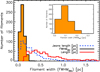Fig. 7 Distribution of deconvolved FWHMdec widths derived from Gaussian fits for the selected sample of 599 filaments (black solid histogram filled in orange). The same histogram is shown in the top right of the panel with a narrower x-axis range. This distribution has a mean of 0.10 pc, a standard deviation of 0.05 pc, a median of 0.09 pc, and an interquartile range of 0.07 pc. For comparison, the blue dashed histogram shows the distribution of central Jeans lengths corresponding to the central column densities of the filaments [${\lambda }_{\text{J}}=c_s^2/\left(G{\Sigma }_0\right)$] for a gas temperature of 10 K. The red histogram shows the distribution of filament lengths. The bin size of all three histograms is 0.06 pc. It can be seen that the distribution of filament widths is much narrower than the other two distributions.

4.2 Properties of filaments along and on either side of their crests

In this section, we discuss the statistical distributions of filament inner widths and background column densities derived from individual column density profiles, taken along and on either side of the filament crests. In practice, the filament properties discussed here were measured on spatially independent radial profiles averaged over 2 × HPBW-long segments along the filament crests (see Sect. 3.1). Figure 11 shows the distributions of individual ${\text{FWHM}}_{\text{dec}}^{\text{pix},\pm }$ and $h{d}_{\text{dec}}^{\text{pix},\pm }$ widths measured along and on either side of the crests for the selected sample of 599 filaments (see Sect. 3.1). For comparison, the distribution of individual Jeans lengths ${\lambda }_J^{\text{pix},\pm }$ corresponding to the background subtracted central column densities along and on either side of the crests is also shown. The ${\text{FWHM}}_{\text{dec}}^{\text{pix},\pm }$ and $h{d}_{\text{dec}}^{\text{pix},\pm }$ distributions are based on 8682 and 8827 independent measurements, respectively (for ~ 2% of the individual profiles, reliable Gaussian fits could not be derived). They have median values of 0.09 and 0.11 pc, respectively, an interquartile range of 0.11 pc in both cases, mean values of 0.13 and 0.14 pc, and standard deviations of 0.12 and 0.11 pc, respectively.These distributions, which measure the statistical importance of possible variations of the inner width along and on either side of the filament crests, peak essentially at the same values as the distributions of median FWHM_dec and hd_dec widths (e.g., Fig. 7). The distributions of individual widths (Fig. 11) exhibit power-law-like tails of values significantly larger than ~ 0.1 pc (see also Panopoulou et al. 2017). Since the distribution of median widths along the filaments (Fig. 7) has a much narrower dispersion around its peak value, it appears that the local inner width of a filament significantly exceeds ~ 0.1 pc at most at afew positions along the filament crest. Such large local excursions of the measured inner width significantly beyond ~ 0.1 pc are averaged out when computing the median filament width. They may be due to several effects. For example, individual profiles along the crest of a filament may be contaminated by (1) the presence of prestellar cores on or slightly off the crest (e.g., Malinen et al. 2012), (2) the presence of fiber-like substructures (e.g,. Hacar et al. 2013, 2018), (3) the intersection points between distinct but overlapping filaments, (4) bad measurements due to disturbed individual profiles, or (5) excursions of the DisPerSE -traced crest connecting two neighboring filaments.

Such excursions about the median width are also seen, albeit less prominently than in Fig. 11, in the distributions of measured individual widths for the tests described in Appendix B, even when the input width is constant along the filament crest (see, e.g., Fig. B.3). Further analyses and tests would be required to estimate the relative contribution of the various possible factors to the shape of the observed distributions of individual ${\text{FWHM}}_{\text{dec}}^{\text{pix},\pm }$ and $h{d}_{\text{dec}}^{\text{pix},\pm }$ widths (Fig. 11). For a given filament in the selected sample, the median absolute deviation of the individual inner widths measured along and on either side of the filament crest ranges between ~ 0.02 and ~ 0.06 pc, which is similar to the dispersions of the distributions of median filament widths measured in each region (cf. Table 3).

To investigate potential asymmetries in the column density profiles of the filaments, we plot in Fig. 12 the distributions of differences in FWHM width ($FWH{M}_{\text{dec}}^{-}-FWH{M}_{\text{dec}}^{+}$) and backgroundcolumn density ($N_{{\text{H}}_2}{}^{\text{bg-}}-N_{{\text{H}}_2}{}^{\text{bg+}}$) between the two sides of each filament crest. Independent estimates of FWHM and $N_{{\text{H}}_2}{}^{\text{bg}}$ on either side of the crest were not possible for 71 filaments. The strongly peaked shape of the distributions in Fig. 12 indicates that a large majority of the filaments in our selected sample exhibit fairly symmetric profiles. The presence of clear wings in the distributions of Fig. 12 nevertheless implies that significant asymmetries in width and $N_{{\text{H}}_2}{}^{\text{bg}}$ exist for some filaments between the two sides of their crests. Interestingly, there is no obvious correlation between an asymmetry detected in filament width and an asymmetry in background column density $N_{{\text{H}}_2}{}^{\text{bg}}$. In other words, a difference in $N_{{\text{H}}_2}{}^{\text{bg}}$ between the two sides (+ and −) of a filament crest does not necessarily imply a difference in FWHM width, and vice versa. A dedicated analysis of filaments with asymmetric profiles would be useful as it may provide valuable constraints on the formation and evolution of filamentary structures in general, as well as their interaction with the parent molecular clouds (see, e.g., Peretto et al. 2012).

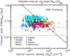Fig. 8 Deconvolved FWHM width against central column density $N_{{\text{H}}_2}{}^0$ for the selected sample of 599 filaments. The dotted horizontal lines mark the spatial resolutions of the column density maps used in the analysis for each field. The solid line running from top left to bottom right shows the central (thermal) Jeans length as a function of central column density [${\lambda }_J=c_s^2/\left(G{\Sigma }_0\right)$] for T = 10 K. The upper x-axis shows an approximate mass per unit length scale derive from the bottom x-axis scale as $M_{\text{line}}={\mu }_{{\text{H}}_2}{m}_{\text{H}}{N}_{{\text{H}}_2}{}^0\times W_{\text{fil}}$ for Wfil = 0.1 pc.

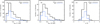Fig. 9 Results of Plummer fits to the median radial column density profiles of the filaments in the selected sample with contrasts C0 > 0.3 and C0 > 1. Panel A: distributions of flat inner diameters Dflat(1) obtained for a fixed value of the Plummer power-law index p = 2 for 260 filaments with C0 > 0.3 (black solid histogram) and 113 filaments with C0 > 1 (blue dashedhistogram). The median Dflat(1) values are 0.13 and 0.10 pc, and the equivalent standard deviations (estimated from scaling the measured IQRs) are 0.10 and 0.08 pc, for the subsets of filaments with C0 > 0.3 and C0 > 1, respectively. Panel B: distributions of Dflat(2) values obtained when p is left as a free parameter (i.e., fitting both Rflat and p) for 199 filaments with C0 > 0.3 and 79 filaments with C0 > 1, respectively. The median Dflat(2) values are 0.15 and 0.12 pc, and the equivalent standard deviations are 0.10 and 0.07 pc, for the subsets of filaments with C0 > 0.3 and C0 > 1, respectively. (NB: The total number of filaments for which reliable Plummer fits can be derived is lower when p and Rflat are fitted simultaneously than when the fit is performed by fixing p = 2.) Panel C: distribution of power-law index values p(2) corresponding to the Dflat(2) values in panel B. The median p(2) value is 2.2 for both subsets of filaments (with C0 > 0.3 and C0 > 1), and the equivalent standard deviations of the distributions are 0.4 and 0.3, respectively.

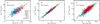Fig. 10 Panel A: mass per unit length integrated over the radial column density profiles, $M_{\text{line}}{}^{\text{int}}$, against median central column density, $N_{{\text{H}}_2}{}^0$, for the 599 filaments of the selected sample. The solid straight line shows the one-parameter best-fit linear relation $M_{\text{line}}{}^{\text{int}}(M_{\odot }/\text{pc})=(0.16\pm 0.05\text{\hspace{0.17em}pc})\times {\Sigma }_{\text{fil}}^0(M_{\odot }/{\text{pc}}^2)$, where ${\Sigma }_{\text{fil}}^0={\mu }_{{\text{H}}_2}{m}_{\text{H}}{N}_{{\text{H}}_2}{}^0$ is the centralgas surface density. Panel B: plot of $M_{\text{line}}{}^{\text{int}}$ against $M_{\text{line}}{}^{\text{w}}~2hr{N}_{{\text{H}}_2}{}^0$ for the same sample of filaments. The one-parameter best-fit linear relation is $M_{\text{line}}{}^{\text{int}}=(1.34\pm 0.03)M_{\text{line}}{}^{\text{w}}$. Panel C: mass per unit length estimated as Mfil∕lfil (where Mfil is calculated summing the column density over the pixels within the area between the filament crest and Rout, after subtraction of $N_{{\text{H}}_2}{}^{\text{bg}}$, see text of Sect. 3.4) against $M_{\text{line}}{}^{\text{int}}$ for the 1310 filaments of the “total” sample. The solid straight line shows the one-parameter best-fit linear relation $M_{\text{fil}}/l_{\text{fil}}~(0.96\pm 0.07)M_{\text{line}}{}^{\text{int}}$.

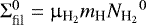
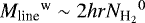
Fig. 11 Distributions of ${\text{FWHM}}_{\text{dec}}^{\text{pix},\pm }$ (black) and $h{d}_{\text{dec}}^{\text{pix},\pm }$ (red) widthsderived from individual profiles along and on either side of the crests for the selected sample of 599 filaments. The median ${\text{FWHM}}_{\text{dec}}^{\text{pix},\pm }$ and $h{d}_{\text{dec}}^{\text{pix},\pm }$ values are 0.09 and 0.11 pc, respectively, and the interquartile range is 0.11 pc for both distributions. The black and red curves show power-law fits to the tails of the ${\text{FWHM}}_{\text{dec}}^{\text{pix},\pm }$ and $h{d}_{\text{dec}}^{\text{pix},\pm }$ distributions, respectively (ΔN∕ΔW ∝ W−2.6±0.5, for both distributions). For comparison, the distribution of Jeans lengths, ${\lambda }_J^{\text{pix},\pm }$, is also shown (blue histogram, cf. Fig. 7).

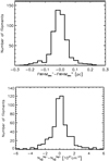Fig. 12 Distributions of the differences in median width ($FWH{M}_{\text{dec}}^{-}-FWH{M}_{\text{dec}}^{+}$, top panel) and median background column density ($N_{{\text{H}}_2}{}^{\text{bg}-}-N_{{\text{H}}_2}{}^{\text{bg}+}$, bottom panel), derived independently on either side of the 599 filament crests in the selected sample. These two distributionshave median ± equivalent standard deviation values of (0.003 ± 0.043) pc and (0.04 ± 0.93) × 1021 cm−2, respectively.

5 Discussion

Our detailed analysis of the radial column density profiles of nearly 600 filamentary structures imaged in eight molecular clouds as part of the HGBS survey confirms and strengthens the result of Arzoumanian et al. (2011) that nearby molecular filaments share a common mean (crest-averaged) inner width of about 0.1 pc, while they span a wide range in central column density $N_{{\text{H}}_2}{}^0$ and mass per unit length M_line⁵ (cf. Figs. 8 and 10). Independent measurements of filament widths in nearby molecular clouds have generally been consistent with our result when obtained through submillimeter dust continuum observations (e.g., Malinen et al. 2012; Ysard et al. 2013; Koch & Rosolowsky 2015; Salji et al. 2015; Rivera-Ingraham et al. 2016, 2017). Measurements obtained using molecular line tracers have been less consistent with our finding, with observations in dense gas tracers such as N₂ H⁺ or NH₃ typically leading to filament widths significantly smaller than 0.1 pc (e.g., Pineda et al. 2011; Fernández-López et al. 2014; Hacar et al. 2018), and studies in low-density tracers such as ¹³CO finding widths significantly larger than 0.1 pc (e.g., Panopoulou et al. 2014). We stress, however, that the dynamic range achieved in (column) density by observations in any given molecular line tracer is lower than that achievable by submillimeter continuum observations, especially from space with, for example, Herschel. This has direct implications for the reliable characterization of the intrinsic column density profiles of filaments. High-density line tracers are typically only sampling gas above a certain critical density and may not probe well the low-density outer parts of filament profiles. Conversely, due to depletion and optical depth effects, low-density gas tracers such as ¹³CO do not probe well the dense inner parts of many molecular filaments.

The filaments analyzed in the present paper span a wide range of column density contrasts C⁰ from ~ 0.1 for the most (thermally) subcritical filaments in our sample to C⁰ ~ 10 for the most thermally supercritical filaments. The filaments with contrasts C⁰ > 1 span a range of central volume densities from a few 10² cm⁻³ to approximately 10⁵ cm⁻³ as inferred from the Plummer fits to their radial column density profiles.

The strong linear correlation between M_line and $N_{{\text{H}}_2}{}^0$ (Fig. 10) suggests that the filaments in our sample are characterized by an effective width given by $W_{\text{fil}}^{\text{eff}}~\text{}(M_{\text{line}}{}^{\text{int}}/M_{\text{line}}{}^{\text{w}})W_{\text{fil}}~\text{}1.3W_{\text{fil}}~\text{}0.13$ pc (see Fig. 10). This result implies that the effective mass (and surface area coverage) of a molecular filament is typically enclosed within a strip of width 1.3 W_fil around the central crest. This value is also consistent with the observed power-law wings for r > W_fil∕2 (see Fig. 3) and the results derived from Plummer fits of the column density profiles (see Fig. 9 and Table 4), suggesting that many molecular filaments have non-Gaussian power-law wings with ρ ~ r⁻² beyond a flat inner plateau (cf. also, e.g., Palmeirim et al. 2013; Cox et al. 2016). On average, however, the non-Gaussian wings contribute little (~ 30%) additional mass. When they are well-developed, the observed power-law wings are shallower than the Ostriker (1964) model (with p = 4) of isothermal filaments in hydrostatic equilibrium.

As already discussed in Arzoumanian et al. (2013), the observational distinction between thermally subcritical and thermally supercriticalfilaments does not correspond to a sharp boundary but to a range of masses per unit length around the theoretical value of M_{line, crit}. For the purposes of this paper, we divide our sample of extracted filaments into three families: thermally subcritical with $M_{\text{line}}^{\text{obs}}\lesssim M_{\text{line},\text{crit}}/2$, “transcritical” filaments with $M_{\text{line},\text{crit}}/2\lesssim M_{\text{line}}^{\text{obs}}\lesssim 2M_{\text{line},\text{crit}}$, and thermally supercritical filaments with M_line ≳ 2 M_line,crit (see Table 5). The three families (subcritical, transcritical, and supercritical) contribute 20%, 51, and 29% of the total gas mass in the whole sample of (1310) filaments, respectively, with significant variations from cloud to cloud (cf. Table 5), as a function of, for example, cloud total dense gas and star-formation activity.

In the selected sample of (599) filaments, 57% of the filaments with column density contrast C⁰ < 1 are thermally subcritical, with a small fraction (4%) being thermally supercritical, while 100% of the filaments with column density contrast C⁰ > 2 are thermally transcritical or supercritical, (Fig. 13 for the selected sample).

Given that our census of filamentary structures is essentially complete to transcritical and supercritical filaments (more than 95% complete for C⁰ ≳ 1 – see Sect. 2.4 and Appendix A), we can estimate the fraction of cloud mass in the form of such filaments. Table 5 gives the total mass in form of filaments in each of the eight clouds. On average, 16% of the total gas mass and about 7% of the total surface area of each cloud is in the form of filaments. A companion paper (Roy et al. 2018) discusses the implications of the relatively low area filling factor of filamentary structures for the power spectrum of cloud images. The above estimate of the fraction of cloud mass in the form of filaments should be considered a lower limit due to the incompleteness of our sample in terms of low-contrast filaments, which may also be contaminated by spurious structures (cf. Appendix A). Incompleteness in terms of subcritical filamentary structures may not have a strong impact on the mass budget in the clouds, however, since the total gas mass in the form of filaments appears to be dominated by transcritical filaments with M_line ~ M_line,crit, which belong to the regime of central column density contrasts C⁰ ≳ 1 where the extracted filament sample is mostly complete (56 and 67% of the filaments with M_line ≳ M_line,crit and M_line ≳ 2 M_line,crit, respectively, have C⁰ > 1, cf. Fig. 13). We refer to André et al. (in prep.) for a detailed discussion of the observed filament mass and M_line distributions.

A dominant fraction ≳ 80% of the dense molecular gas in the clouds is in the form of (mostly supercritical) filaments, where we define dense gas based on column density, that is, $N_{{\text{H}}_2}^{\text{dense}}\ge 7\times {10}^{21}$ cm⁻².

The three families of filaments, defined above on the basis of their M_line as derived from Herschel dust continuum observations, exhibit marked differences in terms of their velocity dispersion and dust polarization properties. Thermally subcritical filaments have sonic or transonic nonthermal velocity dispersions, and are gravitationally unbound with virial parameters (α_vir ≡ M_{line, vir}∕M_line) larger than 2 (e.g., Arzoumanian et al. 2013; Hacar et al. 2016). Their orientations on the plane of the sky are well aligned with the local magnetic field lines (e.g., Planck Collaboration Int. XXXII 2016), and without any star-forming activity. In contrast, thermally supercritical filaments tend to have supersonic velocity dispersions and are self-gravitating with α_vir ~ 1. They tend to be mostly perpendicular to the magnetic field lines observed on large scales in the surrounding ambient cloud (Sugitani et al. 2011; Palmeirim et al. 2013), and are the main sites of prestellar core formation (André et al. 2010; Könyves et al. 2015; Marsh et al. 2016). Transcritical filaments have properties in common with the other two groups. Namely, they tend to have transonic velocity dispersions (Arzoumanian et al. 2013), but are mostly observed perpendicular to the local magnetic field orientation (Cox et al. 2016), and show indications of some star-formation activity (Kainulainen et al. 2016). Indeed, transcritical filaments with M_line close to the thermal value of the critical mass per unit length may be the most appropriate cloud structures for the investigation of the initial conditions of core and star formation (Roy et al. 2015).

Despite marked differences, the three families of filaments all appear to share a common mean inner width. The lack of anti-correlation between filament width and central column density is surprising, since one would naively expect filament widths to scale with local Jeans lengths, represented by the solid line running from top left to bottom right in Fig. 8. Such an anti-correlation would indeed be expected for isothermal filaments in hydrostatic equilibrium (Ostriker 1964). Figure 8 implies that the molecular filaments in our sample are not well described by models of isothermal cylinders in hydrostatic equilibrium⁶.

The existence of a common crest-averaged width ~ 0.1 pc shared by all filaments (at least by the filaments analyzed here) may provide hints on the formation process of filaments. Arzoumanian et al. (2011) suggested that the characteristic filament width may be linked to the sonic scale of turbulence in the cold (~ 10 K) ISM, observed to be around 0.1 pc (Larson 1981; Goodman et al. 1998). The latter appears to be roughly the scale at which supersonic MHD turbulence dissipates and interstellar turbulence turns from supersonic and magnetohydrodynamic on larger scales to subsonic and hydrodynamic on smaller scales (Vázquez-Semadeni et al. 2003; Federrath et al. 2010). Together with the observed subsonic to transonic velocity dispersions of subcritical/critical filaments (Arzoumanian et al. 2013; Hacar et al. 2013, 2016), the common width of filaments suggests that the dissipation of large-scale shock waves (turbulent or not) in the ISM may be important for the formation of the observed filamentary web (see also Inutsuka et al. 2015; Inoue et al. 2018).

The observed correlation between filament mass per unit length and background column density (Fig. 13) indicates some link between filament properties and local conditions in the parent cloud (see also Rivera-Ingraham et al. 2016, 2017). Transcritical and subcritical filaments are observed toward a wide range of background column densities (~ 10²¹ cm${}^{-2}\lesssim N_{{\text{H}}_2}{}^{\text{bg}}\lesssim {10}^{22}$ cm⁻² for transcritical filaments). Only subcritical filaments are found at $N_{{\text{H}}_2}{}^{\text{bg}}\lesssim {10}^{21}$ cm⁻². At the other extreme, thermally supercritical filaments are mostly observed in high-column-density portions of the clouds ($N_{{\text{H}}_2}{}^{\text{bg}}\gtrsim 5\times {10}^{21}$ cm⁻²). This high-density background may represent the reservoir of gas mass from which supercritical filaments appear to accrete while evolving (e.g., Schneider et al. 2012; Hennemann et al. 2012; Arzoumanian et al. 2013; Palmeirim et al. 2013). The physical properties of the ambient cloud may possibly also change during the typical lifetime of filaments due to (single or multiple) interactions with interstellar shock waves (see, e.g., Inutsuka et al. 2015; Arzoumanian et al. 2018).

Thermally supercritical filaments with M_line > 2M_line,crit are expected to be gravitationally unstable to radial contraction and thus should nominally collapse to spindles (Inutsuka & Miyama 1997), which is apparently inconsistent with their characteristic inner width ~ 0.1 pc. A possible explanation is that the non-thermal motions observed toward and along supercritical filaments (Schneider et al. 2010; Arzoumanian et al. 2013; Kirk et al. 2013a; Peretto et al. 2014; Hacar et al. 2017) may provide additional support against gravity and effectively prevent radial contraction. The presence of non-thermal motions is also consistent with models of accretion-driven turbulence within evolving supercritical filaments (Hennebelle & André 2013; Clarke et al. 2016; Inoue et al. 2018). Another key ingredient may be the ambient magnetic field which may act against complete collapse of supercritical filaments, creating ribbon-like, tri-axial structures (Tomisaka 2014; Auddy et al. 2016, Iwasaki et al., in prep.). One limitation of the magnetized ribbon model comes from observational constraints on the maximum AR between the two short axes⁷ of observed filamentary structures, set to first order by the dispersion of measured filament widths.

The very organized magnetic field structure revealed by Planck polarization observations (Planck Collaboration Int. XXXIII 2016) around supercritical filaments suggests that magnetic fields play a dynamically important role in shaping the cold ISM (see also Planck Collaboration Int. XXXV 2016). They may be channeling flows of low-density ambient gas onto star-formingsupercritical filaments, which may be growing in mass per unit length and central column density while fragmenting into prestellar cores (Palmeirim et al. 2013; Arzoumanian et al. 2013; Cox et al. 2016, Shimajiri et al., in prep.). Subcritical filaments, on the otherhand, are not self-gravitating and may be only transient density enhancements, dispersing in a turbulence crossing time ~ 0.3 Myr (for 0.1 pc wide filaments with internal total velocity dispersion of ~ 0.3 km s⁻¹) unless confined by external pressure (Fischera & Martin 2012, Inutsuka et al., in prep.).

While a complete theoretical scenario for the formation and evolution of molecular filaments and their role in the star-formation process is still lacking, the observational results presented in this paper set strong constraints on possible models and represent a challenge for numerical simulations aiming to reproduce realistic filament properties. The existence of a common mean inner width ~ 0.1 pc for filamentary structures also provides hints on the physics at play in the cold ISM and may have strong implications for our understanding of the star-formation process (see André et al. 2014; Roy et al. 2015; Shimajiri et al. 2017; Lee et al. 2017).

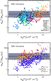Fig. 13 Top panel: mass per unit length $M_{\text{line}}^{\text{int}}$ against background column density $N_{{\text{H}}_2}{}^{\text{bg}}$ for the selected sample of 599 filaments. The horizontal black line corresponds to Mline = Mline,crit = 16 M⊙pc−1, and the grey area shows the transcritical filament regime with $M_{\text{line},\text{crit}}/2\le M_{\text{line}}{}^{\text{int}}\le 2M_{\text{line},\text{crit}}$ (cf. Table 5 and Sect. 5). Bottom panel: same as the top panel, where each dot representing a filament is color coded here as a function of column density contrast C0 (the color code is shown on the bottom right). The percentages of filaments with C0 < 1, 1 < C0 < 2, and C0 > 2 are about 70%, 23%, and 7%, respectively, in the selected sample.

6 Summary and conclusions

In this paper, we present a census of filamentary structures observed in Herschel Gould Belt survey images of eight nearby molecular clouds: IC5146, Orion B, Aquila, Musca, Polaris, Pipe, Taurus L1495, and Ophiuchus. Our method of analysis and main results may be summarized as follows:

• The highly filamentary structure of a nearby molecular cloud imaged with Herschel can be well traced using the DisPerSE algorithm with a persistence threshold PT = rms_min and a robustness threshold RT$=1.5N_{{\text{H}}_2}{}^{\text{bg},\text{min}}$, where rms_min and $N_{{\text{H}}_2}{}^{\text{bg},\text{min}}$ are the minimum rms level of background fluctuations and the minimum background column column density in the input Herschel column density map, respectively. These values for the two main parameters PT and RT of DisPerSE were selected from multiple tests performed on synthetic maps, including realistic populations of mock filaments (see Appendices A and B).

• Using DisPerSE with the above persistence and robustness thresholds, as well as a well-defined procedure (see Sect. 2), we identified a total of 1310 filamentary structures in our eight target fields and a selected sample of 599 filaments with AR ≥ 3 and central column density contrast C⁰ > 0.3. Based on extraction tests performed on synthetic maps (see Appendix A), this selected sample is estimated to be more than 95% completeto filaments with column density contrast C⁰ ≥ 1 (contaminated by ~ 5% of spurious detections), corresponding mostly to thermally transcritical and supercritical filaments with M_line ≳ M_line,crit.

• Filament properties were derived by constructing radial column density radial profiles perpendicular to the filament crests. Without any fitting of the radial profiles, and for each extracted filament, we obtained estimates of the median column density along the filament crest, the outer radius on either side of the crest, the background column density at the outer radius, the filament width from the deconvolved half-power diameter (hd_dec), and the filament length.

• Our sample of nearby molecular filaments is characterized by a narrow distribution of crest-averaged inner widths, with a median hd_dec diameter of 0.10 pc and an interquartile range of 0.08 pc, but spans wide ranges of lengths, column densities, and column density contrasts. The background column densities around the sampled filaments also span a wide range, reflecting significant variations in environmental properties (e.g., external gas pressure). The line-of-sight dust temperatures observed along the filament crests are generally lower than the dust temperature in the background cloud, and the difference in dust temperature is larger for higher column density filaments.

• In addition, the radial column density profiles observed on either side of the filament crests were fitted with Gaussian functions for radii r ∈ [0, 1.5hr], where hr is the half-power radius directly measured on each profile (see above). The resulting distribution of deconvolved, crest-averaged FWHM widths for the 599 filaments in the selected sample is sharply peaked around a median value of 0.10 pc with an interquartile range of 0.07 pc. This distribution is in stark contrast to the much broader distributions of filament lengths and local central Jeans lengths (inversely proportional to the central column densities of the filaments).

• As the observed filaments often feature power-law wings that cannot be well reproduced by Gaussian fits, the radial profiles were also fitted with Plummer-like model functions (Sect. 3.3.2). The resulting distribution of flat inner diameters D_flat = 2 R_flat has a median value of 0.10 pc and an interquartile range of 0.11 pc, in excellent agreement with both the distribution of deconvolved FWHM widths found from Gaussian fitting and the distribution of deconvolved half-power diameters (hd_dec) directly measured on the filament profiles. The power-law exponent p of the underlying density profiles at large radii r > > R_flat is found to have a median value of 2.2 and an equivalent standard deviation of 0.3. Finally, filaments with central column density contrasts C⁰ > 1 are found to span a range of central volume densities from a few 10² cm⁻³ to approximately 10⁵ cm⁻³.

• Our method of estimating filament properties from the radial column density profiles was validated by performing tests on synthetic cloud maps, including populations of mock filaments with both Gaussian and Plummer-like input radial profiles (see Appendix B).

• The distributions of individual $h{d}_{\text{dec}}^{\text{pix},\pm }$ and ${\text{FWHM}}_{\text{dec}}^{\text{pix},\pm }$ widths, derived from independent profiles taken along and on either side of the filament crests, have the same median and mean values as the distributions of hd_dec and FWHM_dec widths averaged along and on either side of the filament crests. They exhibit larger dispersions about their mean, however, with power-law-like tails of values significantly larger than 0.1 pc. These unusually large values of the $h{d}_{\text{dec}}^{\text{pix},\pm }$ and ${\text{FWHM}}_{\text{dec}}^{\text{pix},\pm }$ widths may result from (1) physical variations of properties along each filament crest, (2) local variations in the background cloud, and/or (3) bad measurements due to locally disturbed radial profiles. Further analysis and tests would be needed to assess the relative contribution of these different factors to the observed distributions.

• Our filament sample can be divided into three families: thermally subcritical filaments with M_line ≲ 0.5 M_line,crit, transcritical filaments with 0.5 M_line,crit ≲ M_line ≲ 2 M_line,crit, and thermally supercritical filaments with M_line ≳ 2 M_line,crit. Transcritical filaments contribute more than half of the total gas mass of the whole sample of extracted filaments. On average, 16% of the total mass in the target clouds is in the form of filaments and about 80% of the dense gas mass (at $N_{{\text{H}}_2}>7\times {10}^{21}$ cm⁻²) is in the form of (mostly transcritical and supercritical) filaments.

• The masses per unit length derived for the sampled filaments correlate very well with their central column densities, which is consistent with the existence of a characteristic filament width.

• These results suggest that, contrary to expectations, dense supercritical filaments with M_line > 2M_line,crit do not collapse radially to spindles but somehow maintain a crest-averaged width of ~ 0.1 pc while evolving and fragmenting into prestellar cores.

Acknowledgements

D.A. acknowledges an International Research Fellowship from the Japan Society for the Promotion of Science (JSPS). This work has received support from the European Research Council under the European Union’s Seventh Framework Programme (ERC Advanced Grant Agreement no. 291294 - ORISTARS). A.R. and N.S. acknowledge support by the french ANR and the german DFG through the project “GENESIS” (ANR-16-CE92-0035-01/DFG1591/2-1). The present study has made use of data from the Herschel Gould Belt survey (HGBS) project (http://gouldbelt-herschel.cea.fr). The HGBS is a Herschel Key Programme jointly carried out by SPIRE Specialist Astronomy Group 3 (SAG 3), scientists of several institutes in the PACS Consortium (CEA Saclay, INAF-IFSI Rome and INAF-Arcetri, KU Leuven, MPIA Heidelberg), and scientists of the Herschel Science Center (HSC).

Appendix A: Completeness of the extracted filament sample

In this appendix, we discuss several tests performed on synthetic data to estimate the completeness of the extracted filament sample following the method described in Sect. 2.

To test our method of tracing filaments, synthetic column density maps of filamentary molecular clouds were generated by adding realistic populations of mock filaments to a Herschel column density map where most, if not all, compact sources and filamentary structures had been removed using the getsources and getfilaments algorithms (Men’shchikov et al. 2012; Men’shchikov 2013).

We built the background column density map (see Fig. A.1a) by periodically duplicating the lower half of the Herschel column density image of the Aquila cloud (cf. Fig. 1 of Könyves et al. 2015) resulting in a 4° × 2° map corresponding to ~ 18.5 pc × 9.2 pc at a distance d = 260 pc. Synthetic filaments were generated using a real filament crest traced with DisPerSE in the Aquila cloud. Starting from this observed crest used as a template, the synthetic filaments were given a Gaussian column density profile with a fixed width FHWM = 0.1 pc at d = 260 pc and random orientations with respect to the Cartesian x- and y-axes of the background map. For each realization, a group of 100 such synthetic filaments was distributed randomly over the background column density map, controlling the contrast C⁰ between themedian column density along the crest of each synthetic filament and the local background column density (see Fig. A.1c). A large number of such realizations were generated and the same method as described in Sect. 2 for identifying filamentary structures in the real data was applied in each case.

As mentioned in Sect. 2.2, the completeness of our filament extractions was estimated by investigating the variation of the fraction of extracted synthetic filaments as a function of input filament contrast, C⁰, and AR, for several values of the persistence threshold, PT, and robustness threshold, RT, of the DisPerSE run (see Sect. 2.2).

Ten synthetic maps, each including 100 Gaussian-shaped filaments giving a total of 1000 synthetic filaments, were generated for each combination of the above mentioned four parameters (C⁰, AR, PT, RT). Figure A.1c shows an example of one of these realizations.

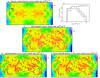Fig. A.1 Panel a: “background” map used in our tests of filament extraction, corresponding to a 4° × 2° portion of a Herschel column density map after subtraction of compact sources and filamentary structures with the getsources and getfilaments algorithms (Men’shchikov et al. 2012; Men’shchikov 2013). The vertical double arrow indicates the1° scale of the map and is the same on all the maps of this figure. The spatial resolution of the maps is 0.023 pc, corresponding to 18′′ at a distance of 260 pc. Panel b: column density histograms of the “background map” in panel a using two different bin sizes, Sbin = 1021 cm−2 (solid histogram) and Sbin = 1020 cm−2 (dashed histogram). The minimum background column density, $N_{{\text{H}}_2}{}^{\text{bg},\text{min}}$, and the minimum level of background fluctuations, rmsmin, used to adjust the DisPerSE parameters RT and PT (see text) were estimated from the median and standard deviation of column density values in the first bin of the solid histogram, respectively: $N_{{\text{H}}_2}{}^{\text{bg},\text{min}}=2.5\times {10}^{21}$cm−2 and rmsmin = 0.19 × 1021cm−2. Panel c: example of a synthetic column density map obtained by distributing 100 synthetic filaments with contrast C0 = 1 and AR = 10 over the “background map” of panel a. Here, all synthetic filaments were given a Gaussian profile with FWHM = 0.1 pc and a length of ~ 1 pc at the distance of 260 pc. Panel d: as in panel c but with the filament crests traced with DisPerSE overlaid in black. DisPerSE was run with a persistence threshold PT = rmsmin and a robustness threshold RT $=1.5N_{{\text{H}}_2}{}^{\text{bg},\text{min}}$. Panel e: as in panel d but after removing filament segments shorter than ten times the HPBW beam, i.e., after “cleaning” the DisPerSE skeleton (cf. Sect. 2.3). The white crests indicate the structures identified as “spurious” (four in this case), while the black crests correspond to “true” filaments.

We then applied the filament extraction method of Sect. 2 to each realization. Since, as mentioned in Sect. 2.3, a good choice for PT is on the order of the background column density fluctuations, PT was varied as follows: rms_min∕2, rms_min, 2 rms_min, 4 rms_min, where rms_min is the minimum rms in the background column density map (see Fig. A.1b). As for the robustness threshold, it was varied between RT$=0.75N_{{\text{H}}_2}{}^{\text{bg},\text{min}}$ and RT$=2.25N_{{\text{H}}_2}{}^{\text{bg},\text{min}}$, where $N_{{\text{H}}_2}{}^{\text{bg},\text{min}}$ is the minimum $N_{{\text{H}}_2}{}^{\text{bg}}$ in the background column density map, since it is linked to the minimum column density contrast of the filaments to be extracted, RT$~\text{}{C}^0{N}_{{\text{H}}_2}{}^{\text{bg}}$ (cf., Sect. 2.3). Finally, for each realization, we estimated the number of “true” mock filaments that were recovered using our method of filament tracing, as well as the number of “spurious”⁸ extracted structures. To do so, we compared the crests traced by DisPerSE with the input skeleton maps. When a DisPerSE crest matched a crest from the input skeleton (numbered from 1 to 100 in each of the realizations) for at least 30 pixels (corresponding to 5 × HPBW), the DisPerSE crest was considered a “true” detection. When the DisPerSE crest did not have a counterpart in the input skeleton for at least 30 pixels, the DisPerSE crest was flagged as a “spurious” detection (see e.g., Fig. A.1e).

We define the fraction of extracted filaments as the ratio of the number of “true” detections to the number of input filaments, i.e., 1000, for each combination of the four studied parameters (C⁰, AR, PT, RT). The fraction of “spurious” detections is defined as the ratio of the number of “spurious” detections to the total number of (“true”+“spurious”) detections.

Figure A.2 shows the statistics of “true” and “spurious” detections, based on a total of 1000 synthetic filaments for each set of PT and RT values. Here, the synthetic filaments all have an AR = 10 and column density contrasts C⁰ = 1 (left panel) or C⁰ = 2 (right panel).

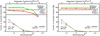Fig. A.2 Left panel: fractions of “true” detections (solid color lines) and “spurious” detections (dotted color lines) in tests of filament extractions as a function of the robustness threshold RT used with DisPerSE (in units of $N_{{\text{H}}_2}{}^{\text{bg}}$ on the bottom x-axis and 1021cm−2 on the top x-axis), for four values of the persistence threshold PT (0.5 rmsmin, rmsmin, 2 rmsmin, 4 rmsmin, color coded as shown at the top right of the plot). The synthetic filaments used in these tests all had Gaussian profiles with FWHM = 0.1 pc, an AR = 10, a column density contrast C0 = 1 over the background, and were distributed in the map shown in Fig. A.1a. The statistics shown in the plot are based on a total of 1000 such synthetic filaments for each set of the two DisPerSE parameters RT and PT. The two horizontal black lines indicate completeness levels of 70% and 90%, respectively. Right panel: as in left panel but for synthetic filaments with intrinsic column density contrast C0 = 2 over the background.

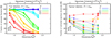Fig. A.3 Left panel: fractions of “true” detections (solid color lines) in tests of filament extraction as a function of the robustness threshold RT used with DisPerSE (in units of $N_{{\text{H}}_2}{}^{\text{bg}}$ on the bottom x-axis and 1021cm−2 on the top x-axis), for three values of the input (AR = 3, 5, 10 – see symbols at the bottom left of the plot) and four values of the input column density contrast (C0 = 0.3, 0.5, 0.7, 1, 2 – color coded as shown at the top right of the plot). The statistics shown in this plot are based on a total of 1000 synthetic filaments with Gaussian profiles of FWHM = 0.1 pc for each set of (AR, C0) input values, added to the background map shown in Fig. A.1a. The persistence threshold used in DisPerSE was fixed to PT = rmsmin. Right panel:as in left panel but for the fractions of “spurious” detections (dotted color lines).

Thermally subcritical filaments are expected to have column density contrasts C⁰ ≲ 1, while thermally transcritical/supercritical filaments should have C⁰ > 1 (see Sect. 2.4). As an illustration, filaments with intrinsic column density contrast C⁰ = 1 and Gaussian width FWHM = 0.1 pc, embedded in a background cloud with $N_{{\text{H}}_2}{}^{\text{bg}}=2.5\times {10}^{21}$cm⁻² (for ${\text{μ}}_{{\text{H}}_2}=2.8$), have a mass per unit length M_line = 11 M_⊙pc⁻¹.

For all input filament contrasts C⁰, the fractions of extracted synthetic filaments were found to be almost independent of the persistence threshold for PT values within a factor of two of the minimum rms in the background column density map, rms_min. The fraction of extracted synthetic filaments with C⁰ = 2 is larger than 95% for robustness threshold values RT$\le 2.25N_{{\text{H}}_2}{}^{\text{bg},\text{min}}$. The same level of completeness is achieved for synthetic filaments with C⁰ = 1 when RT$\le 1.5N_{{\text{H}}_2}{}^{\text{bg},\text{min}}$. The fraction of extracted synthetic filaments with C⁰ = 1 decreases below 95% when RT$>1.5N_{{\text{H}}_2}{}^{\text{bg},\text{min}}$ but nevertheless remains ≥ 80% for RT$\le 2N_{{\text{H}}_2}{}^{\text{bg},\text{min}}$.

The fraction of “spurious” detections behaves in the opposite way, that is, it decreases when RT increases. “Spurious” detections correspond to cirrus-like column density structures in the background column density map. These structures are traced by DisPerSE but are not “true” filamentary structures. For RT$\ge 1.5N_{{\text{H}}_2}{}^{\text{bg},\text{min}}$, the fraction of spurious extracted structures is less than 10%, but it increases rapidly for RT$<1.5N_{{\text{H}}_2}{}^{\text{bg},\text{min}}$.

We also investigated the effect of the robustness parameter RT on the fractions of extracted synthetic filaments and “spurious” detections for AR < 10 and column density contrasts C⁰ < 1. The plots of Fig. A.3 show the fractions of extracted synthetic filaments and “spurious” structures for mock filaments with 0.3 ≤ C⁰ ≤ 2 and 3 ≤ AR ≤ 10, as a function of RT for a fixed persistence threshold PT = rms_min. It can be seen that the fraction of extracted synthetic filaments is almost independent (within 10%) of filament 3 ≤ AR < 10, but decreases significantly when C⁰ decreases for RT$<N_{{\text{H}}_2}{}^{\text{bg},\text{min}}$. The fraction of “spurious” detections is almost constant (within 15%) for all C⁰ > 0.5 and AR > 3 values, and decreases when RT increases. For C⁰ ≤ 0.5 and AR ≤ 3, the fraction of “spurious” extracted structures exceeds ~ 50% of the total number of detections.

Appendix B: Reliability of derived filament properties

Here, we assess the reliability of our method of estimating filament properties using the measurement steps described in Sect. 3. To this end, synthetic maps including mock filaments with Gaussian and Plummer-like column density radial profiles, and various distributions of input properties, such as inner width, power-law slope at large radii, and filament contrast, were constructed. Several sets of synthetic maps were generated by distributing between 60 and 180 mock filaments with given input properties (AR, C⁰, p) within the background column density map of Fig. A.1A, which has a spatial resolution of 0.023 pc corresponding to ~ 18′′ at a distance of 260 pc. The mock filaments were distributed in an ordered way and at well-separated locations to reduce measurement uncertainties due to possible intersections or blending between filaments. The filament crests of the synthetic maps were traced using DisPerSE with PT = rms_min and RT$=1.5N_{{\text{H}}_2}{}^{\text{bg},\text{min}}$ following the steps described in Sect. 2, and analyzed in the same way as the real data as explained in Sect. 3.

Figure B.1 compares the distributions of input and measured filament properties derived without any fitting of the column density radial profiles and after determination of the filament crest, outer radius, and background column density values, as explained in Sects. 2 and 3. The distribution of measured half-power diameters, hd, for filaments with Gaussian profiles has a median value consistent with the input FWHM width of the mock filaments (Fig. B.1A). The input filament contrasts and central/background column densities are also well recovered.

In the following two subsections (Sects. B.1 and B.2), we discuss the reliability of inner width measurements derived from Gaussian and Plummer fits to the filament radial profiles, respectively. We summarize the results of these tests in Sect. B.3.

B.1 Synthetic filaments with Gaussian input radial column density profiles

As illustrated in Fig. 3 (panels a and b), some filaments are observed to have radial column density profiles that are reasonably well described by a Gaussian profile. To discuss the accuracy of deriving the inner widths of such filaments, we generated a number of synthetic maps by distributing identical Gaussian-shaped mock filaments with AR = 10 and column density contrast C⁰ = 1, within the background column density map of Fig. A.1a. The effective spatial resolution of all synthetic maps was 0.023 pc (i.e., ~ 18′′ at 260 pc).

We used four distributions of Gaussian-shaped synthetic filaments:

• a)

  All mock filaments had the same input FWHM width, uniform along each filament crest (Figs. B.2A and B.3A).

• b)

  The sample of mock filaments had a power-law distribution of FWHM widths between 0.03 and 0.25 pc, and a slope of − 2 in ΔN∕Δlog(FWHM) (180 input mock filaments were used in this case – Fig. B.2B).

• c)

  The number of mock filaments per linear bin of width was constant in the range 0.03 pc ≤ FWHM ≤ 0.4 pc. i.e., flat distribution of input widths, (Fig. B.2C).

• d)

  The mock filaments had a Gaussian distribution of FWHM widths along their crests, with a mean value of 0.1 pc and a standard deviation of 0.05 pc (Figs. B.3B and B.3C).

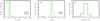Fig. B.1 Histograms of derived crest-averaged properties (half-power diameter, hd, in panel a; filament contrast, C0, in panel b; background-subtracted central column density, $N_{{\text{H}}_2}{}^0$, in panel c) in measurement tests using a population of Gaussian mock filaments. The vertical dashed lines in panels a and b indicate the fixed input properties of the mock filaments: FWHM width (W = 0.1 pc) and column density contrast (C0 = 1). In panel c, the black and green histograms show the distribution of input and derived background-subtracted column densities averaged along the filament crests, respectively.

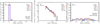Fig. B.2 Histograms of FWHM widths derived from Gaussian fitting to the radial column density profiles of synthetic filaments with Gaussian input profiles and fixed input FWHM width (W = 0.1 pc; (panel a), a power law distribution of FWHM widths between 0.03 and 0.25 pc (panel b), and a flat input distribution of FWHM widths between 0.03 and 0.4 pc (panel c). The input FWHM width distributions are shown with the black dashed lines on all panels. Results are presented for four choices of the fitting range (1.5hr, 2.0hr, 2.5hr, 3.0hr), color codedas shown on the right hand side of each plot (cf. Sect. 3.3.3). Note how the measured distributions of filament widths are almost independent of the fitting range.

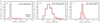Fig. B.3 Histograms of FWHM widths derived from Gaussian fits to the column density profiles of Gaussian-shaped synthetic filaments. The distributions of input and measured FWHM widths are displayed in black and red, respectively. The range radii used for the Gaussian fits was [0, 1.5hr]. Panel a: distribution of individual FWHM widths measured along and on either side of the filament crests for input FWHM width (W = 0.1 pc) constant along the filament length (same as Fig. B.2A). Panel b: distribution of individual FWHM widths measured along and on either side of the filament crests, for input individual FWHM widths with a Gaussian distribution centered at 0.1 pc with a standard deviation of 0.05 pc. Panel c: distribution of median FWHM widths “averaged” over each filament crest for the same input FWHM distribution as in panel B.

Figure B.2 shows the distribution of measured FWHM widths derived from Gaussian fitting to the radial column density profiles of Gaussian-shaped mock filaments for three input distributions of filament FWHM widths (constant, power-law, and flat, respectively). A peaked distribution of measured FWHM widths was obtained solely when the input mock filaments had the same FWHM value constant along their crest (Fig. B.2A). Likewise, a power-law distribution of measured FWHM widths was obtained only when the input mock filaments had a power-law distribution of FWHM widths (Fig. B.2B), and a flat distribution of measured FWHM widths was obtained only when the input distribution was flat (Fig. B.2C).

We can also see that reliable filament widths can be measured down to ~ 0.03 pc, corresponding to the smallest input width considered, close to the 0.023 pc resolution of the synthetic column density map. The slope of the input power-law distribution of mock filament widths was recovered with an accuracy better than ~ 10% (for all fitting ranges).

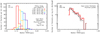Fig. B.4 Histograms of FWHM widths derived from Gaussian fitting to the radial column density profiles of synthetic filaments with Plummer radial profiles and input contrast C0 = 1. Panel a: all input 180 mock filaments had Plummer radial profiles with 2Rflat = Dflat = 0.1 pc and p = 2. Results are presented for four choices of the fitting range, [0,1.5hr], [0,2.0hr], [0,2.5hr], and [0,3.0hr], color coded as shown at the top right of the plot (cf. Sect. 3.3.3). We note how the measured distribution of filament widths depends on the fitting range (the median filament width derived for each fitting range is given at the top right of the plot). Panel b: input 180 mock filaments had Plummer radial profiles with a power-law distribution of Dflat diameters between 0.03 and 0.25 pc (same distribution as the distribution of FWHMwidths in Fig. B.2B) and a Gaussian distribution of p values with a mean of 2 and a standard deviation of 0.3. The FWHM widths were derived from Gaussian fits to the radial column density profiles with a fitting range of [0,1.5hr]. The solid black and red straight lines show power-law fits to the input and measured distributions of widths, respectively.

Figure B.3A shows the distribution of individual FWHM widths measured along and on either side of the filament crests for an input width of 0.1 pc constant along the crests (same as Fig. B.2A). The median value of the measured widths is consistent with the input constant width, but a tail of larger values can also be seen on the distribution. These excursions from the constant input width may be attributed to bad measurements and/or spurious structures.

Figures B.3B and B.3C show the results of Gaussian width measurements when the input FWHM widths are not strictly constant along each filament crest, but have a Gaussian distribution with a mean value of 0.1 pc and a standard deviation of 0.05 pc. Figure B.3B shows the distribution of individual FWHM widths derived from Gaussian fitting to the individual profiles along and on either side of the filament crests, while Fig. B.3C shows the distribution of median FWHM values derived after “averaging” the independent measurements obtained along and on either side of each filament crest (see Sects. 3.1 and 3.2). The derived distributions of individual FWHM widths and of median (crest-averaged) FWHM widths are both consistent with the corresponding input distributions. We also note that the standard deviation of the derived distribution of median FWHM widths is larger when the input individual FWHM widths have a Gaussian distribution about a mean value (Fig. B.3C) than when the input FWHM width is constant along each filament crest (Fig. B.2A), i.e., 0.02 and < 0.01 pc, respectively.

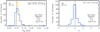Fig. B.5 Results of measurements performed to test the reliability of Plummer fits to the radial column density profiles of Plummer-shaped synthetic filaments with fixed input central column density contrast C0 = 1, inner diameter Dflat = 0.1 pc, and power-law index p = 2. The input Dflat and p values are marked by vertical dashed lines on the plots. The synthetic filaments are the same as those used in Fig. B.4. Two sets of results are provided for Dflat in panel a, depending on whether the power-law index p of the Plummer model profile was fixed to p = 2 [(1), yellow histogram] or left as a free parameter [(2), blue histogram]. The blue histogram of fitted p values in panel b corresponds to the blue distribution of Dflat(2) values in panel a. The median values of the derived parameters as well as their equivalent standard deviations (scaled from the measured IQRs) are provided at the top right of the panels.

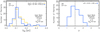Fig. B.6 As in Fig. B.5 but for Plummer-shaped synthetic filaments with fixed input central column density contrast C0 = 0.5. The input Plummer parameters were fixed to Dflat = 0.1 pc and p = 2, as marked by vertical dashed lines on the plots.

The FWHM widths derived from Gaussian fitting to the profiles of Gaussian-shaped synthetic filaments are not affected by the range of radii used for fitting the radial column density profiles. As expected and as already mentioned in Sect. 3.3.3, however, the fitting range does matter when Gaussian fits are used to estimate the FWHM widths of filaments with Plummer-like input column density profiles. This is discussed in the following section.

B.2 Synthetic filaments with Plummer input radial density profiles

The logarithmic radial column density profiles of many observed filaments are characterized by a flat inner plateau up to a radius R_flat and non-Gaussian wings for r > > R_flat (see, e.g., Fig. 3). Using a Plummer-like model profile (see Eq. (5)), one can in principle reproduce the behavior of the radial column density distribution for both r ≤ R_flat and r > > R_flat, which is notpossible with a Gaussian fit.

In this section, we present measurement tests to assess the reliability of deriving the inner widths of filaments with Plummer-like radial column density profiles, using both Gaussian and Plummer-like function fits (as described in Sects. 3.3.1 and 3.3.2, respectively). For this purpose, several synthetic maps were constructed by distributing, within the background column density map of Fig. A.1A at a spatial resolution of 0.023 pc, a population of Plummer-shaped mock filaments with input column density contrasts of C⁰ = 1 and C⁰ = 0.5, and various input distributions of D_flat = 2R_flat and p values.

We used the following distributions of Plummer-like synthetic filaments: a) All mock filaments had the same R_flat and p values, constant along each filament crest. Three sets of synthetic maps were considered, with mock filaments having D_flat = 0.1 pc and p = 1.5, 2, and 3, respectively (Figs. B.4A, Fig. B.5–B.7).

b) All mock filaments had the same power-law index p = 2, but a flat distribution of D_flat (i.e., a constant number of mock filaments per linear bin of D_flat) in the range 0.03 pc ≤ R_flat ≤ 0.34 pc (Fig. B.8A).

c) All mock filaments had the same D_flat = 0.1 pc diameter, but a flat distribution of p values (i.e., a constant number of mock filaments per linear bin of p) in the range 1.5 ≤ p ≤ 3.2 (Fig. B.9).

d) The mock filaments had a power-law distribution of D_flat diameters between 0.03 pc and 0.25 pc, with a power-law index of − 2 (in ΔN∕Δlog(D_flat)) and a Gaussian distribution of p values with a mean of 2 and a standard deviation of 0.3 (Fig. B.4B, and B.8B).

e) The mock filaments had the same p = 2 index and a power-law distribution of individual D_flat diameters along their crests with a power-law index of − 2 (in ΔN∕Δlog(D_flat)) between 0.022 pc and 0.19 pc (Fig. B.10).

Figure B.4A shows the distributions of FWHM widths derived from Gaussian fits to the radial column density profiles of Plummer-shaped mock filaments with uniform input D_flat = 0.1 pc and p = 2 parameters. For the same input D_flat and p values, the derived FWHM widths increase for increasing fitting range, for example, from [0,1.5hr] to [0,3hr] (cf. also, Sect. 3.3.3 and Fig. 4). This is also the case when the input mock filaments have p = 1.5 and p = 3 (not illustrated here with a figure). For a given fitting range and input D_flat diameter, the measured FWHM widths from Gaussian fits to Plummer-like input column density profiles decrease for increasing p: for example, for a fitting range of 0 ≤ r ≤ 1.5hr, $FWHM=1.4(D_{\text{flat}}^{p=1.5})$, $FWHM=1.1(D_{\text{flat}}^{p=2})$, and $FWHM=0.8(D_{\text{flat}}^{p=3})$, when p = 1.5, p = 2, and p = 3, respectively. The logarithmic slope of the power-law profile, p, also influences the derived values of the half-power diameter, hd. Our tests show that for the same input D_flat radius, the median value of the hd distribution decreases when the input p index increases: $hd=1.8(D_{\text{flat}}^{p=1.5})$, $hd=1.4(D_{\text{flat}}^{p=2})$, and $hd=0.98(D_{\text{flat}}^{p=3})$, for p = 1.5, p = 2, and p = 3, respectively.

Figure B.4B shows the distribution of FWHM widths derived from Gaussian fitting to the radial profiles of 180 Plummer-shaped mock filaments with a power-law distribution of input D_flat diameters between 0.03 pc and 0.25 pc and a Gaussian distribution of p values with a mean of 2 and a standard deviation of 0.3. For a fitting range of 0 ≤ r ≤ 1.5hr, the derived distribution of FWHM widths is in good agreement with the input distribution of filament inner widths down to 0.03 pc, close to the spatial resolution of the synthetic background map. The logarithmic slope of the fitted power-law distribution of FWHM widths is only ~ 15% shallower than that of the input distribution of D_flat diameters.

Figures B.5 and B.6 show the results of Plummer fitting to the profiles of Plummer-shaped filaments with input contrasts C⁰ = 1 and C⁰ = 0.5, respectively. In the C⁰ = 1 case, the derived D_flat and p parameters have peaked distributions with median values consistent with the input parameters. In the lower contrast case (C⁰ = 0.5), the median values of the derived D_flat and p distributions tend to be slightly larger than the corresponding input values, and the dispersions of D_flat and p values are about 30 and 40% larger, respectively, than the dispersions measured for C⁰ = 1. These larger uncertainties in the results of Plummer fitting for input filaments with C⁰ = 0.5 may be attributed to less well-defined power-law profiles at r > > R_flat for low-contrast filaments leading to larger errors in the fitted parameters.

Figure B.7 shows the results of Plummer-fitting measurements for an input population of Plummer-shaped mock filaments with fixed input parameters: D_flat = 0.1 pc and p = 1.5 (panels a and b) or p = 3 (panels c and d). It can be seen that when p and D_flat are fitted simultaneously, the input p and D_flat values are reasonably well recovered. When the fitting is performed with fixing the power-law exponent to p = 2, different from the input value p = 1.5 or p = 3, the derived R_flat values are larger or smaller (by up to ~ 50%) than the input D_flat = 0.1 pc radius, respectively.

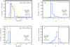Fig. B.7 As in Fig. B.5 for Plummer-shaped synthetic filaments with fixed input central column density contrast C0 = 1, inner diameter Dflat = 0.1 pc, and power-law index p = 1.5 (top panels, a and b) or p = 3 (bottom panels, c and d). The input Dflat and p values are marked by vertical dashed lines in the plots. The left panels, a and c, histograms of measured Dflat values, whilethe right panels, b and d, show histograms of measured p values.

Figure B.8A shows that a flat distribution of D_flat values is derived when the input mock filaments have a flat distribution of D_flat diameters. Likewise, Fig. B.8B shows that a power law distribution of D_flat values is derived when the input mock filaments have a power-law distribution of D_flat diameters. Correct estimates of the D_flat diameter are derived down to 0.03 pc, close to the spatial resolution of the synthetic map. Furthermore, when both D_flat and p are fitted simultaneously, the median value of the derived p indices is compatible with the input p value in both sets of experiments.

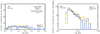Fig. B.8 Results of Plummer fits to Plummer-shaped synthetic filaments with a central column density contrast C0 = 1 and two distributions of Dflat inner diameters [flat in panel a; power law in panel b]. Two sets of Dflat measurements are provided depending on whether the power-law index p of the Plummer model profile was fixed to p = 2 [(1), yellow histogram] or left as a free parameter [(2), blue histogram]. The input distribution of Dflat values are shown by the black dashed histogram in both panels. In the left panel a, the input mock filaments had a fixed input p = 2 and a flat input distribution of Dflat between 0.03 pc and 0.34 pc. In the right panel b, the input mock filaments had a power-law distribution of Dflat diameters between 0.03 and 0.25 pc, similar to the distribution of FWHM widths in Fig. B.2B and B.4B, and a Gaussian distribution of p values witha mean of 2 and a standard deviation of 0.3. The power-law slopes of the measured distributions of Dflat diameters (shown as yellow and blue straight lines for the Dflat(1) and Dflat(2) estimates, respectively) are only ~ 30% shallower than the slope of the input distribution (black straight line).

Figure B.9 shows that a flat distribution of p values is obtained when the input mock filaments have a flat distribution of p indices from 1.5 to 3.2 and a fixed D_flat diameter. When p and D_flat are fitted simultaneously in this case, the distribution of derived D_flat values peaksat the constant input D_flat value. The derived distribution of D_flat radii has a larger dispersion when the fitting is performed while fixing p to 2, different from the input p values.

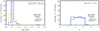Fig. B.9 As in Fig. B.5 for Plummer-shaped synthetic filaments with a fixed central column density contrast C0 = 1, a fixed input Dflat = 0.1 pc diameter (dashed black straight line in the left panel), and a flat distribution of input p values between 1.5 and 3.2 (dashed black histogram in the right panel).

Figure B.10 shows the results of measurement tests obtained from both Plummer (panel a) and Gaussian (panels b and c) fitting for a sample of Plummer-shaped mock filaments with variable input D_flat values along their crests. In these tests, each synthetic filament was given a power-law distribution of D_flat values along its crest. (The distribution of median, crest-averaged D_flat diameters for the sample of 180 input filaments also followed a power law.) it can be seen that the distribution of derived median D_flat values (Fig. B.10A) and the distribution of derived median FWHM widths (Fig. B.10B) are both consistent with the input distributions down to ~ 0.025 pc, close to the resolution of the background column density map. Figure B.10C shows that the distribution of individual FWHM widths measured along the filament crests (before averaging) reproduces well the input distribution of individual D_flat diameters.

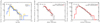Fig. B.10 Results of measurements performed to test the reliability of inner-width estimates from both Plummer and Gaussian fits to the profiles of 180 Plummer-shaped synthetic filaments with variable Dflat diameters along the crests. The synthetic filaments had a fixed input central column density contrast C0 = 1, a fixed indexp = 2, and a power-law distribution of individual input Dflat diameters between 0.022 pc and 0.19 pc with an exponent of − 2 (in ΔN∕ΔlogW, similar to that in Fig. B.4B) along each crest. The distribution of input inner diameters is shownby a dashed black histogram in all three plots. Left panel: histograms of measured Dflat diameters from Plummer fitting. Two sets of results are provided for Dflat as explained in the caption of Fig. B.5. Middle panel: histogram of median FWHM values derived from Gaussian fits after averaging along each filament crest. Right panel: histograms of individual FWHM values measured along the filament crests. In this plot, the dashed black histogram of input Dflat values has been rescaled so as to have the same peak as the red histogram of measured Dflat values.

B.3 Summary and conclusions regarding the reliability of filament width estimates

The inner widths of filaments with Gaussian-like intrinsic profiles are estimated reliably by both 1) our method of deriving the half-power diameter without any fitting (Sect. 3.2) and 2) the FWHM widths derived from Gaussian fits to the observed profiles (Sect. 3.3.1). The latter FWHM estimates are not affected by the fitting range for Gaussian-shaped filaments. For a fixed input width constant along the filament crest, the distribution of individual FWHM widths derived along and on either side of the filament crests show some excursion from the median value of the distribution (consistent with the input fixed value), that may be attributed to bad measurements and/or spurious structures. Considering crest-averaged values result in median filament widths that are robust in the presence of measurement errors.

The inner widths of filaments with Plummer-like intrinsic profiles can be estimated 1) without any fitting (hd estimates), 2) with Gaussian function fitting (FWHM estimates), and 3) Plummer function fitting (D_flat = 2R_flat estimates). The first two estimates, hd and FWHM, are affected by the power-law index p of the Plummer profile: for the same input D_flat diameter, hd and FWHM both increase for decreasing intrinsic p values. For the same p index, the dispersion of the derived FWHM widths is smaller than that of the derived hd values. While the derived FWHM widths depend on the fitting range, they are closest to the input D_flat diameters, and therefore provide satisfactory estimates of the filament inner widths of filaments, when the fitting range is chosen to be 0 ≤ r ≤ 1.5hr. For this fitting range, the derived FWHM widths provide accurate estimates of the D_flat diameters to better than ~ 50% (for filaments with C⁰ > 1) when 1.5 < p < 3. The D_flat diameters derived from Plummer fitting provide satisfactory estimates of the intrinsic inner diameters of Plummer-shaped filaments when the filament contrasts are large enough (e.g., C⁰ ≳0.5). Furthermore, such D_flat estimates do not have significant biases in the sense that the input distributions of D_flat diameters are correctly reproduced in tests performed on populations of Plummer-shaped synthetic filaments, independently of the shape of the input distributions (e.g., constant, flat, or power law). For constant input D_flat diameters, the dispersion of measured values increases 1) when the column density contrast of the input filaments decreases and 2) when D_flat and p are fitted simultaneously.

Appendix C: Column density maps and filament skeletons

This appendix presents the column density maps of the entire fields analyzed in this paper for seven of the eight target clouds (see Table 1 for an overview of the target clouds). The column density map of the entire field analyzed in the eighth target cloud (IC5146) is shown in the right panel of Fig. 1. These column density maps were derived from HGBS data⁹ as explained in Sect. 2.3. The skeletons of the entire sample of filaments traced in each cloud as explained in Sect. 2.2 are shown as cyan or dark blue solid curves in the column density maps. These skeleton maps are available in fits format¹⁰. The cyan curves trace the crests of the selected sample of filaments derived as explained in Sect. 3.5 (cf., Table 2).

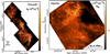Fig. C.1 Herschel column density maps of the Orion B field (left panel – Könyves et al. 2018) and Aquila field (right panel – Könyves et al. 2015) analyzed in this paper, as derived from HGBS data (http://gouldbelt-herschel.cea.fr/archives, André et al. 2010). The effective HPBW resolution is 18.′′ 2. The crests of the filamentary structures traced in the two clouds using DisPerSE (see Sect. 2.2) are overlaid as solid curves. The cyan curves trace the filament crests of the selected sample, and the dark blue curves trace the additional filament crests in the extended sample (cf. Sect. 3.5). See Table 2 for the absolute values of the persistence and robustness thresholds of the DisPerSE runs, as well as the number of extracted filaments in each field.

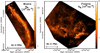Fig. C.2 A sin Fig. B.11 but for the Musca cloud (left panel; see Cox et al. 2016) and Polaris cloud (right panel; see Ward-Thompson et al. 2010; Miville-Deschênes et al. 2010).

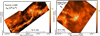Fig. C.3 As in Fig. B.11 but for the Taurus/L1495 cloud (left panel; Palmeirim et al. 2013; Marsh et al. 2016)and the Ophiuchus L1688/L1689 field (right panel; Ladjelate et al., in prep.).

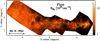Fig. C.4 As in Fig. B.11 but for the Pipe molecular cloud (Peretto et al. 2012, Roy et al., in prep.). The labels indicate the offsets in degrees relative to the center of the map at RA(J2000) = 17:38:20 and Dec(J2000) = 27:02:25. The X–Y reference frame is rotated by − 37° with respectto the RA–Dec reference frame (counting positive angles east of north).

References

All Tables

All Figures

Fig. 1 Herschel column density maps of a portion of the analyzed region in Orion B (left panel) and of the entire field analyzed here in IC5146 (right panel), as derived from HGBS data (http://gouldbelt-herschel.cea.fr/archives; cf. André et al. 2010; Arzoumanian et al. 2011; Könyves et al. in prep.). The effective HPBW resolution of these maps is 18.′′ 2. The crests of the filamentary structures traced in the two clouds using DisPerSE as explained in Sect. 2.2 are overlaid as solid curves. The cyan blue curves trace the filament crests of the selected sample, and the dark blue curves trace the crests of additional filaments from the extended sample (cf. Sect. 3.5 and Table 2). The maps of the other fields analyzed in this paper are shown in Appendix C.

In the text

Fig. 2 Fromleft to right columns: median radial column density profile observed on either side of the filament axis in lin-lin format (panels A), median radial column density profile on the left-hand side of the crest (i.e., r < 0 in A1 andA2) in log-log format (panels B), and panels C: logarithmic slope of the column density profile ($\text{d\hspace{0.17em}ln}{N}_{{\text{H}}_2}/\text{d\hspace{0.17em}ln}r$) as a function of radius from the central crest, for a filament in the Ophiuchus cloud (top three panels, A1, B1, C1) and a filament in the Taurus cloud (bottom three panels, A2, B2, C2). In Cols. A and B, the yellow area/error bars correspond to the median absolute deviation (mad(r)) of the distributions of independent cuts taken perpendicular to the filament crest (see Sect. 3.1). In Col. A, the outer radii $R_{\text{out}}^{\pm }$ (vertical dotted red line) and the background column densities $N_{{\text{H}}_2}{}^{\text{bg}}\pm$ (horizontal red line) are marked. In Col. B, the observational beam of 18.2′′ (blue curve), the outer radius $R_{\text{out}}^{-}$ (vertical dotted red line), the background column density $N_{{\text{H}}_2}{}^{\text{bg}}-$ (horizontal red line), and the half power radius hr− (vertical dotted yellow line) are shown. As explained in Sect. 3.2, the values of $R_{\text{out}}^{\pm }$, $N_{{\text{H}}_2}{}^{\text{bg}}\pm$, and hr± were derived from the data independently on either side of the filament crest, using the logarithmic slope plot Col. C smoothed over 3 × HPBW. In Col. C, the black solid curve represents the logarithmic slope profile at the original resolution, while the blue symbols show the logarithmic slope profile smoothed over 3 × HPBW; the red dotted vertical line marks the derived outer radius $R_{\text{out}}^{-}$, and the black dotted horizontal line marks a zero slope (flat column density profile).

In the text

References

- Abergel, A., Boulanger, F., Mizuno, A., & Fukui, Y. 1994, ApJ, 423, L59 [NASA ADS] [CrossRef] [Google Scholar]
- Alves de Oliveira, C., Schneider, N., Merín, B., et al. 2014, A&A, 568, A98 [NASA ADS] [CrossRef] [EDP Sciences] [Google Scholar]
- André, P., Di Francesco, J., Ward-Thompson, D., et al. 2014, Protostars and Planets VI (Tucson, AZ: University Press of Arizona) 27 [Google Scholar]
- André, P., Men’shchikov, A., Bontemps, S., et al. 2010, A&A, 518, L102 [NASA ADS] [CrossRef] [EDP Sciences] [Google Scholar]
- André, P., Revéret, V., Könyves, V., et al. 2016, A&A, 592, A54 [NASA ADS] [CrossRef] [EDP Sciences] [Google Scholar]
- Arzoumanian, D. 2012, Ph.D. Thesis, Université Paris Diderot (Paris VII) [Google Scholar]
- Arzoumanian, D., André, P., Didelon, P., et al. 2011, A&A, 529, L6 [Google Scholar]
- Arzoumanian, D., André, P., Peretto, N., & Könyves, V. 2013, A&A, 553, A119 [NASA ADS] [CrossRef] [EDP Sciences] [Google Scholar]
- Arzoumanian, D., Shimajiri, Y., Inutsuka, S.-i., Inoue, T., & Tachihara, K. 2018, PASJ, 70, 96 [NASA ADS] [CrossRef] [Google Scholar]
- Auddy, S., Basu, S., & Kudoh, T. 2016, ApJ, 831, 46 [NASA ADS] [CrossRef] [Google Scholar]
- Bally, J., Lanber, W. D., Stark, A. A., & Wilson, R. W. 1987, ApJ, 312, L45 [NASA ADS] [CrossRef] [Google Scholar]
- Benedettini, M., Schisano, E., Pezzuto, S., et al. 2015, MNRAS, 453, 2036 [NASA ADS] [CrossRef] [Google Scholar]
- Bontemps, S., André, P., Könyves, V., et al. 2010, A&A, 518, L85 [NASA ADS] [CrossRef] [EDP Sciences] [Google Scholar]
- Cambrésy, L. 1999, A&A, 345, 965 [NASA ADS] [Google Scholar]
- Clark, S. E., Peek, J. E. G., & Putman, M. E. 2014, ApJ, 789, 82 [NASA ADS] [CrossRef] [Google Scholar]
- Clarke, S. D., Whitworth, A. P., & Hubber, D. A. 2016, MNRAS, 458, 319 [NASA ADS] [CrossRef] [Google Scholar]
- Cox, N. L. J., Arzoumanian, D., André, P., et al. 2016, A&A, 590, A110 [NASA ADS] [CrossRef] [EDP Sciences] [Google Scholar]
- Falgarone, E., Pety, J., & Phillips, T. G. 2001, ApJ, 555, 178 [NASA ADS] [CrossRef] [Google Scholar]
- Federrath, C. 2016, MNRAS, 457, 375 [NASA ADS] [CrossRef] [Google Scholar]
- Federrath, C., Roman-Duval, J., Klessen, R. S., Schmidt, W., & Mac Low M. 2010, A&A, 512, A81 [NASA ADS] [CrossRef] [EDP Sciences] [Google Scholar]
- Fernández-López, M., Arce, H. G., Looney, L., et al. 2014, ApJ, 790, L19 [NASA ADS] [CrossRef] [Google Scholar]
- Fischera, J., & Martin, P. G. 2012, A&A, 542, A77 [NASA ADS] [CrossRef] [EDP Sciences] [Google Scholar]
- Goodman, A. A., Barranco, J. A., Wilner, D. J., & Heyer, M. H. 1998, ApJ, 504, 223 [NASA ADS] [CrossRef] [Google Scholar]
- Green, C.-E., Cunningham, M. R., Dawson, J. R., et al. 2017, ApJ, 840, L17 [NASA ADS] [CrossRef] [Google Scholar]
- Hacar, A., Kainulainen, J., Tafalla, M., Beuther, H., & Alves, J. 2016, A&A, 587, A97 [NASA ADS] [CrossRef] [EDP Sciences] [Google Scholar]
- Hacar, A., Tafalla, M., & Alves, J. 2017, A&A, 606, A123 [NASA ADS] [CrossRef] [EDP Sciences] [Google Scholar]
- Hacar, A., Tafalla, M., Forbrich, J., et al. 2018, A&A, 610, A77 [NASA ADS] [CrossRef] [EDP Sciences] [Google Scholar]
- Hacar, A., Tafalla, M., Kauffmann, J., & Kovács, A. 2013, A&A, 554, A55 [NASA ADS] [CrossRef] [EDP Sciences] [Google Scholar]
- Harvey, P. M., Huard, T. L., Jørgensen, J. K., et al. 2008, ApJ, 680, 495 [NASA ADS] [CrossRef] [Google Scholar]
- Hennebelle, P. 2013, A&A, 556, A153 [NASA ADS] [CrossRef] [EDP Sciences] [Google Scholar]
- Hennebelle, P., & André, P. 2013, A&A, 560, A68 [NASA ADS] [CrossRef] [EDP Sciences] [Google Scholar]
- Hennebelle, P., Banerjee, R., Vázquez-Semadeni, E., Klessen, R. S., & Audit, E. 2008, A&A, 486, L43 [NASA ADS] [CrossRef] [EDP Sciences] [Google Scholar]
- Hennemann, M., Motte, F., Schneider, N., et al. 2012, A&A, 543, L3 [NASA ADS] [CrossRef] [EDP Sciences] [Google Scholar]
- Hill, T., Motte, F., Didelon, P., et al. 2011, A&A, 533, A94 [NASA ADS] [CrossRef] [EDP Sciences] [Google Scholar]
- Hill, T., Motte, F., Didelon, P., et al. 2012, A&A, 542, A114 [NASA ADS] [CrossRef] [EDP Sciences] [Google Scholar]
- Hily-Blant, P., & Falgarone, E. 2009, A&A, 500, L29 [NASA ADS] [CrossRef] [EDP Sciences] [Google Scholar]
- Inoue, T., Hennebelle, P., Fukui, Y., et al. 2018, PASJ, 70, S53 [NASA ADS] [Google Scholar]
- Inutsuka, S., & Miyama, S. M. 1997, ApJ, 480, 681 [NASA ADS] [CrossRef] [Google Scholar]
- Inutsuka, S.-i., Inoue, T., Iwasaki, K., & Hosokawa, T. 2015, A&A, 580, A49 [NASA ADS] [CrossRef] [EDP Sciences] [Google Scholar]
- Joncas, G., Boulanger, F., & Dewdney, P. E. 1992, ApJ, 397, 165 [NASA ADS] [CrossRef] [Google Scholar]
- Juvela, M., Ristorcelli, I., Pagani, L., et al. 2012, A&A, 541, A12 [NASA ADS] [CrossRef] [EDP Sciences] [Google Scholar]
- Kainulainen, J., Hacar, A., Alves, J., et al. 2016, A&A, 586, A27 [NASA ADS] [CrossRef] [EDP Sciences] [Google Scholar]
- Kauffmann, J., Bertoldi, F., Bourke, T. L., Evans, II, N. J., & Lee, C. W. 2008, A&A, 487, 993 [NASA ADS] [CrossRef] [EDP Sciences] [Google Scholar]
- Kirk, H., Myers, P. C., Bourke, T. L., et al. 2013a, ApJ, 766, 115 [NASA ADS] [CrossRef] [Google Scholar]
- Kirk, J. M., Ward-Thompson, D., Palmeirim, P., et al. 2013b, MNRAS, 432, 1424 [NASA ADS] [CrossRef] [Google Scholar]
- Koch, E. W., & Rosolowsky, E. W. 2015, MNRAS, 452, 3435 [NASA ADS] [CrossRef] [Google Scholar]
- Könyves, V., André, P., Men’shchikov, A., et al. 2010, A&A, 518, L106 [NASA ADS] [CrossRef] [EDP Sciences] [Google Scholar]
- Könyves, V., André, P., Men’shchikov, A., et al. 2015, A&A, 584, A91 [NASA ADS] [CrossRef] [EDP Sciences] [Google Scholar]
- Lada, C. J., Forbrich, J., Lombardi, M., & Alves, J. F. 2012, ApJ, 745, 190 [NASA ADS] [CrossRef] [Google Scholar]
- Larson, R. B. 1981, MNRAS, 194, 809 [NASA ADS] [CrossRef] [Google Scholar]
- Lee, Y.-N., Hennebelle, P., & Chabrier, G. 2017, ApJ, 847, 114 [NASA ADS] [CrossRef] [Google Scholar]
- Li, D., & Goldsmith, P. F. 2012, ApJ, 756, 12 [NASA ADS] [CrossRef] [Google Scholar]
- Li, G.-X., Urquhart, J. S., Leurini, S., et al. 2016, A&A, 591, A5 [NASA ADS] [CrossRef] [EDP Sciences] [Google Scholar]
- Mac Low, M., & Klessen, R. S. 2004, Rev. Mod. Phys., 76, 125 [NASA ADS] [CrossRef] [Google Scholar]
- Malinen, J., Juvela, M., Rawlings, M. G., et al. 2012, A&A, 544, A50 [NASA ADS] [CrossRef] [EDP Sciences] [Google Scholar]
- Marsh, K. A., Griffin, M. J., Palmeirim, P., et al. 2014, MNRAS, 439, 3683 [NASA ADS] [CrossRef] [Google Scholar]
- Marsh, K. A., Kirk, J. M., André, P., et al. 2016, MNRAS, 459, 342 [NASA ADS] [CrossRef] [Google Scholar]
- McClure-Griffiths, N. M., Dickey, J. M., Gaensler, B. M., Green, A. J., & Haverkorn, M. 2006, ApJ, 652, 1339 [NASA ADS] [CrossRef] [Google Scholar]
- Men’shchikov, A. 2013, A&A, 560, A63 [NASA ADS] [CrossRef] [EDP Sciences] [Google Scholar]
- Men’shchikov, A., André, P., Didelon, P., et al. 2010, A&A, 518, L103 [NASA ADS] [CrossRef] [EDP Sciences] [Google Scholar]
- Men’shchikov, A., André, P., Didelon, P., et al. 2012, A&A, 542, A81 [NASA ADS] [CrossRef] [EDP Sciences] [Google Scholar]
- Miville-Deschênes, M., Martin, P. G., Abergel, A., et al. 2010, A&A, 518, L104 [NASA ADS] [CrossRef] [EDP Sciences] [Google Scholar]
- Miville-Deschênes, M.-A., Duc, P.-A., Marleau, F., et al. 2016, A&A, 593, A4 [NASA ADS] [CrossRef] [EDP Sciences] [Google Scholar]
- Molinari, S., Swinyard, B., Bally, J., et al. 2010, A&A, 518, L100 [NASA ADS] [CrossRef] [EDP Sciences] [Google Scholar]
- Myers, P. C. 2009, ApJ, 700, 1609 [NASA ADS] [CrossRef] [EDP Sciences] [Google Scholar]
- Nakamura, F.,& Li, Z. 2008, ApJ, 687, 354 [NASA ADS] [CrossRef] [Google Scholar]
- Ntormousi, E., Hennebelle, P., André, P., & Masson, J. 2016, A&A, 589, A24 [NASA ADS] [CrossRef] [EDP Sciences] [Google Scholar]
- Ortiz-León, G. N., Dzib, S. A., Kounkel, M. A., et al. 2017, ApJ, 834, 143 [NASA ADS] [CrossRef] [Google Scholar]
- Ostriker, J. 1964, ApJ, 140, 1056 [NASA ADS] [CrossRef] [MathSciNet] [Google Scholar]
- Palmeirim, P., André, P., Kirk, J., et al. 2013, A&A, 550, A38 [NASA ADS] [CrossRef] [EDP Sciences] [Google Scholar]
- Panopoulou, G. V., Psaradaki, I., Skalidis, R., Tassis, K., & Andrews, J. J. 2017, MNRAS, 466, 2529 [NASA ADS] [CrossRef] [Google Scholar]
- Panopoulou, G. V., Tassis, K., Goldsmith, P. F., & Heyer, M. H. 2014, MNRAS, 444, 2507 [NASA ADS] [CrossRef] [Google Scholar]
- Peretto, N., André, P., Könyves, V., et al. 2012, A&A, 541, A63 [NASA ADS] [CrossRef] [EDP Sciences] [Google Scholar]
- Peretto, N., Fuller, G. A., André, P., et al. 2014, A&A, 561, A83 [NASA ADS] [CrossRef] [EDP Sciences] [Google Scholar]
- Pilbratt, G. L., Riedinger, J. R., Passvogel, T., et al. 2010, A&A, 518, L1 [CrossRef] [EDP Sciences] [Google Scholar]
- Pineda, J. E., Goodman, A. A., Arce, H. G., et al. 2011, ApJ, 739, L2 [NASA ADS] [CrossRef] [Google Scholar]
- Planck Collaboration Int. XXXII. 2016, A&A, 586, A135 [NASA ADS] [CrossRef] [EDP Sciences] [Google Scholar]
- Planck Collaboration Int. XXXIII. 2016, A&A, 586, A136 [NASA ADS] [CrossRef] [EDP Sciences] [Google Scholar]
- Planck Collaboration Int. XXXV. 2016, A&A, 586, A138 [NASA ADS] [CrossRef] [EDP Sciences] [Google Scholar]
- Rivera-Ingraham, A., Ristorcelli, I., Juvela, M., et al. 2016, A&A, 591, A90 [NASA ADS] [CrossRef] [EDP Sciences] [Google Scholar]
- Rivera-Ingraham, A., Ristorcelli, I., Juvela, M., et al. 2017, A&A, 601, A94 [NASA ADS] [CrossRef] [EDP Sciences] [Google Scholar]
- Roy, A., André, P., Arzoumanian, D., et al. 2018, A&A, submitted [Google Scholar]
- Roy, A., André, P., Arzoumanian, D., et al. 2015, A&A, 584, A111 [NASA ADS] [CrossRef] [EDP Sciences] [Google Scholar]
- Roy, A., André, P., Palmeirim, P., et al. 2014, A&A, 562, A138 [NASA ADS] [CrossRef] [EDP Sciences] [Google Scholar]
- Roy, A., Martin, P. G., Polychroni, D., et al. 2013, ApJ, 763, 55 [NASA ADS] [CrossRef] [Google Scholar]
- Salji, C. J., Richer, J. S., Buckle, J. V., et al. 2015, MNRAS, 449, 1782 [NASA ADS] [CrossRef] [Google Scholar]
- Schisano, E., Rygl, K. L. J., Molinari, S., et al. 2014, ApJ, 791, 27 [NASA ADS] [CrossRef] [Google Scholar]
- Schlafly, E. F., Green, G., Finkbeiner, D. P., et al. 2014, ApJ, 786, 29 [NASA ADS] [CrossRef] [Google Scholar]
- Schlafly, E. F., Green, G., Finkbeiner, D. P., et al. 2015, ApJ, 799, 116 [NASA ADS] [CrossRef] [Google Scholar]
- Schneider, N., André, P., Könyves, V., et al. 2013, ApJ, 766, L17 [NASA ADS] [CrossRef] [Google Scholar]
- Schneider, N., Csengeri, T., Bontemps, S., et al. 2010, A&A, 520, A49 [NASA ADS] [CrossRef] [EDP Sciences] [Google Scholar]
- Schneider, N., Csengeri, T., Hennemann, M., et al. 2012, A&A, 540, L11 [NASA ADS] [CrossRef] [EDP Sciences] [Google Scholar]
- Schneider, S., & Elmegreen, B. G. 1979, ApJS, 41, 87 [NASA ADS] [CrossRef] [Google Scholar]
- Shimajiri, Y., André, P., Braine, J., et al. 2017, A&A, 604, A74 [NASA ADS] [CrossRef] [EDP Sciences] [Google Scholar]
- Smith,R. J., Glover, S. C. O., & Klessen, R. S. 2014, MNRAS, 445, 2900 [NASA ADS] [CrossRef] [Google Scholar]
- Smith, R. J., Glover, S. C. O., Klessen, R. S., & Fuller, G. A. 2016, MNRAS, 455, 3640 [NASA ADS] [CrossRef] [Google Scholar]
- Sousbie, T. 2011, MNRAS, 414, 350 [NASA ADS] [CrossRef] [Google Scholar]
- Sousbie, T., Pichon, C., & Kawahara, H. 2011, MNRAS, 414, 384 [NASA ADS] [CrossRef] [Google Scholar]
- Sugitani, K., Nakamura, F., Watanabe, M., et al. 2011, ApJ, 734, 63 [Google Scholar]
- Toalá, J. A., Vázquez-Semadeni, E., & Gómez, G. C. 2012, ApJ, 744, 190 [NASA ADS] [CrossRef] [Google Scholar]
- Tomisaka, K. 2014, ApJ, 785, 24 [NASA ADS] [CrossRef] [Google Scholar]
- Vázquez-Semadeni, E., Ballesteros-Paredes, J., & Klessen, R. S. 2003, ApJ, 585, L131 [NASA ADS] [CrossRef] [Google Scholar]
- Vázquez-Semadeni, E., Gómez, G. C., Jappsen, A. K., et al. 2007, ApJ, 657, 870 [NASA ADS] [CrossRef] [Google Scholar]
- Wang, K., Testi, L., Ginsburg, A., et al. 2015, MNRAS, 450, 4043 [NASA ADS] [CrossRef] [MathSciNet] [Google Scholar]
- Ward-Thompson, D., Kirk, J. M., André, P., et al. 2010, A&A, 518, L92 [NASA ADS] [CrossRef] [EDP Sciences] [Google Scholar]
- Ysard, N., Abergel, A., Ristorcelli, I., et al. 2013, A&A, 559, A133 [NASA ADS] [CrossRef] [EDP Sciences] [Google Scholar]
The derived filament skeleton maps are available in fits format from http://gouldbelt-herschel.cea.fr/archives
The  and Mline values derived here overestimate the intrinsic central column densities and masses per unit length of the observed filaments by ~ 60% on average, assuming random inclination angles of the filaments with respect to the plane of the sky (cf. Arzoumanian et al. 2011, 2013). The plots and values given in the tables of this paper are not corrected for this inclination effect.
Significantly steeper power-law density profiles than the p ~ 2 profiles found here for r > > Rflat have been observed in N2H+ or NH3 by, e.g., Pineda et al. (2011) and Hacar et al. (2018) who reported p ~ 4, in agreement with the isothermal equilibrium model of Ostriker (1964). As pointed out earlier, however, high-density gas tracers such as N2H+ or NH3 lines may not be sensitive to the low-density outer parts of filament profiles, biasing the derived p index toward larger values.
A ribbon-like filamentary structure (e.g., Auddy et al. 2016) has one long axis, the main axis of the filament, and two short axes: one is set by hydrostatic equilibrium and corresponds to the Jeans length, and the other two by magnetohydrostatic equilibrium, resulting in an hourglass shape.
All Tables
Fractions of subcritical, transcritical, and supercritical filaments, along with filament mass and area filling factors in each cloud.