| Issue |
A&A
Volume 594, October 2016
Planck 2015 results
|
|
|---|---|---|
| Article Number | A3 | |
| Number of page(s) | 32 | |
| Section | Cosmology (including clusters of galaxies) | |
| DOI | https://doi.org/10.1051/0004-6361/201526998 | |
| Published online | 20 September 2016 | |
Planck 2015 results
III. LFI systematic uncertainties
1 APC, AstroParticule et Cosmologie, Université Paris Diderot, CNRS/IN2P3, CEA/lrfu, Observatoire de Paris, Sorbonne Paris Cité, 10 rue Alice Domon et Léonie Duquet, 75205 Paris Cedex 13, France
2 African Institute for Mathematical Sciences, 6–8 Melrose Road, Muizenberg, 7945 Cape Town, South Africa
3 Agenzia Spaziale Italiana Science Data Center, via del Politecnico snc, 00133 Roma, Italy
4 Aix-Marseille Université, CNRS, LAM (Laboratoire d’Astrophysique de Marseille) UMR 7326, 13388 Marseille, France
5 Astrophysics Group, Cavendish Laboratory, University of Cambridge, J J Thomson Avenue, Cambridge CB3 0HE, UK
6 CGEE, SCS Qd 9, Lote C, Torre C, 4° andar, Ed. Parque Cidade Corporate, CEP 70308-200 Brasília, DF, Brazil
7 CITA, University of Toronto, 60 St. George St., Toronto, ONM5S3H8, Canada
8 CNRS, IRAP, 9 Av. colonel Roche, BP 44346, 31028 Toulouse Cedex 4, France
9 California Institute of Technology, Pasadena, CA 91125, USA
10 Centro de Estudios de Física del Cosmos de Aragón (CEFCA), Plaza San Juan, 1, planta 2, 44001 Teruel, Spain
11 Computational Cosmology Center, Lawrence Berkeley National Laboratory, Berkeley, CA 94720, USA
12 DSM/Irfu/SPP, CEA-Saclay, 91191 Gif-sur-Yvette Cedex, France
13 DTU Space, National Space Institute, Technical University of Denmark, Elektrovej 327, 2800 Kgs. Lyngby, Denmark
14 Département de Physique Théorique, Université de Genève, 24 quai E. Ansermet, 1211 Genève 4, Switzerland
15 Departamento de Astrofísica, Universidad de La Laguna (ULL), 38206 La Laguna, Tenerife, Spain
16 Departamento de Física, Universidad de Oviedo, Avda. Calvo Sotelo s/n, 33003 Oviedo, Spain
17 Departamento de Matemáticas, Estadística y Computación, Universidad de Cantabria, Avda. de los Castros s/n, 39005 Santander, Spain
18 Department of Astrophysics/IMAPP, Radboud University Nijmegen, PO Box 9010, 6500 GL Nijmegen, The Netherlands
19 Department of Physics & Astronomy, University of British Columbia, 6224 Agricultural Road, Vancouver, British Columbia, Canada
20 Department of Physics and Astronomy, Dana and David Dornsife College of Letter, Arts and Sciences, University of Southern California, Los Angeles, CA 90089, USA
21 Department of Physics and Astronomy, University College London, London WC1E 6BT, UK
22 Department of Physics, Florida State University, Keen Physics Building, 77 Chieftan Way, Tallahassee, FL 32306, USA
23 Department of Physics, Gustaf Hällströmin katu 2a, University of Helsinki, 00100 Helsinki, Finland
24 Department of Physics, Princeton University, Princeton, NJ 08544, USA
25 Department of Physics, University of California, Santa Barbara, CA 93106, USA
26 Department of Physics, University of Illinois at Urbana-Champaign, 1110 West Green Street, Urbana, Illinois, USA
27 Dipartimento di Fisica e Astronomia G. Galilei, Università degli Studi di Padova, via Marzolo 8, 35131 Padova, Italy
28 Dipartimento di Fisica e Scienze della Terra, Università di Ferrara, via Saragat 1, 44122 Ferrara, Italy
29 Dipartimento di Fisica, Università La Sapienza, P.le A. Moro 2, Roma, Italy
30 Dipartimento di Fisica, Università degli Studi di Milano, via Celoria, 16 Milano, Italy
31 Dipartimento di Fisica, Università degli Studi di Trieste, via A. Valerio 2, 24128 Trieste, Italy
32 Dipartimento di Matematica, Università di Roma Tor Vergata, via della Ricerca Scientifica, 1 Roma, Italy
33 Discovery Center, Niels Bohr Institute, Blegdamsvej 17, 2100 Copenhagen, Denmark
34 European Space Agency, ESAC, Planck Science Office, Camino bajo del Castillo, s/n, Urbanización Villafranca del Castillo, Villanueva de la Cañada, 28692 Madrid, Spain
35 European SpaceAgency, ESTEC, Keplerlaan 1, 2201 AZ Noordwijk, The Netherlands
36 Gran Sasso Science Institute, INFN, viale F. Crispi 7, 67100 L’ Aquila, Italy
37 HGSFP and University of Heidelberg, Theoretical Physics Department, Philosophenweg 16, 69120 Heidelberg, Germany
38 Haverford College Astronomy Department, 370 Lancaster Avenue, Haverford, Pennsylvania, USA
39 Helsinki Institute of Physics, Gustaf Hällströmin katu 2, University of Helsinki, 00100 Helsinki, Finland
40 INAF−Osservatorio Astrofisico di Catania, via S. Sofia 78, Catania, Italy
41 INAF−Osservatorio Astronomico di Padova, Vicolo dell’Osservatorio 5, 35122 Padova, Italy
42 INAF−Osservatorio Astronomico di Roma, via di Frascati 33, 00078 Monte Porzio Catone, Italy
43 INAF−Osservatorio Astronomico di Trieste, via G.B. Tiepolo 11, 34131 Trieste, Italy
44 INAF/IASF Bologna, via Gobetti 101, 40127 Bologna, Italy
45 INAF/IASF Milano, via E. Bassini 15, 20133 Milano, Italy
46 INFN, Sezione di Bologna, via Irnerio 46, 40126 Bologna, Italy
47 INFN, Sezione di Roma 1, Università di Roma Sapienza, P.le Aldo Moro 2, 00185 Roma, Italy
48 INFN, Sezione di Roma 2, Università di Roma Tor Vergata, via della Ricerca Scientifica, 1 Roma, Italy
49 INFN/National Institute for Nuclear Physics, via Valerio 2, 34127 Trieste, Italy
50 IUCAA, Post Bag 4, Ganeshkhind, Pune University Campus, 411007 Pune, India
51 Imperial College London, Astrophysics group, Blackett Laboratory, Prince Consort Road, London, SW7 2AZ, UK
52 Infrared Processing and Analysis Center, California Institute of Technology, Pasadena, CA 91125, USA
53 Institut d’Astrophysique Spatiale, CNRS, Univ. Paris-Sud, Université Paris-Saclay, Bât. 121, 91405 Orsay Cedex, France
54 Institut d’Astrophysique de Paris, CNRS (UMR 7095), 98bis boulevard Arago, 75014 Paris, France
55 Institute of Astronomy, University of Cambridge, Madingley Road, Cambridge CB3 0HA, UK
56 Institute of Theoretical Astrophysics, University of Oslo, Blindern, 0371 Oslo, Norway
57 Instituto de Astrofísica de Canarias, C/Vía Láctea s/n, La Laguna, 38205 Tenerife, Spain
58 Instituto de Física de Cantabria (CSIC-Universidad de Cantabria), Avda. de los Castros s/n, 39005 Santander, Spain
59 Istituto Nazionale di Fisica Nucleare, Sezione di Padova, via Marzolo 8, 35131 Padova, Italy
60 Jet Propulsion Laboratory, California Institute of Technology, 4800 Oak Grove Drive, Pasadena, California, USA
61 Jodrell Bank Centre for Astrophysics, Alan Turing Building, School of Physics and Astronomy, The University of Manchester, Oxford Road, Manchester, M13 9PL, UK
62 Kavli Institute for Cosmological Physics, University of Chicago, Chicago, IL 60637, USA
63 Kavli Institute for Cosmology Cambridge, Madingley Road, Cambridge, CB3 0HA, UK
64 Kazan Federal University, 18 Kremlyovskaya St., 420008 Kazan, Russia
65 LAL, Université Paris-Sud, CNRS/IN2P3, Orsay, France
66 LERMA, CNRS, Observatoire de Paris, 61 avenue de l’Observatoire, 75104 Paris, France
67 Laboratoire AIM, IRFU/Service d’Astrophysique − CEA/DSM − CNRS − Université Paris Diderot, Bât. 709, CEA-Saclay, 91191 Gif-sur-Yvette Cedex, France
68 Laboratoire de Physique Subatomique et Cosmologie, Université Grenoble-Alpes, CNRS/IN2P3, 53 rue des Martyrs, 38026 Grenoble Cedex, France
69 Laboratoire de Physique Théorique, Université Paris-Sud 11 & CNRS, Bâtiment 210, 91405 Orsay, France
70 Lawrence Berkeley National Laboratory, Berkeley, CA 94720, USA
71 Max-Planck-Institut für Astrophysik, Karl-Schwarzschild-Str. 1, 85741 Garching, Germany
72 National University of Ireland, Department of Experimental Physics, Maynooth, Co. Kildare, Ireland
73 Nicolaus Copernicus Astronomical Center, Bartycka 18, 00-716 Warsaw, Poland
74 Niels Bohr Institute, Blegdamsvej 17, Copenhagen, Denmark
75 SISSA, Astrophysics Sector, via Bonomea 265, 34136 Trieste, Italy
76 SMARTEST Research Centre, Università degli Studi e-Campus, via Isimbardi 10, 22060 Novedrate (CO), Italy
77 School of Physics and Astronomy, Cardiff University, Queens Buildings, The Parade, Cardiff, CF24 3AA, UK
78 Space Sciences Laboratory, University of California, Berkeley, California, USA
79 Special Astrophysical Observatory, Russian Academy of Sciences, Nizhnij Arkhyz, Zelenchukskiy region, 369167 Karachai-Cherkessian Republic, Russia
80 Sub-Department of Astrophysics, University of Oxford, Keble Road, Oxford OX1 3RH, UK
81 UPMC Univ Paris 06, UMR 7095, 98bis boulevard Arago, 75014 Paris, France
82 Université de Toulouse, UPS-OMP, IRAP, 31028 Toulouse Cedex 4, France
83 University of Granada, Departamento de Física Teórica y del Cosmos, Facultad de Ciencias, 18010 Granada, Spain
84 University of Granada, Instituto Carlos I de Física Teórica y Computacional, 18010 Granada, Spain
85 Warsaw University Observatory, Aleje Ujazdowskie 4, 00-478 Warszawa, Poland
Received: 19 July 2015
Accepted: 8 February 2016
Abstract
We present the current accounting of systematic effect uncertainties for the Low Frequency Instrument (LFI) that are relevant to the 2015 release of the Planck cosmological results, showing the robustness and consistency of our data set, especially for polarization analysis. We use two complementary approaches: (i) simulations based on measured data and physical models of the known systematic effects; and (ii) analysis of difference maps containing the same sky signal (“null-maps”). The LFI temperature data are limited by instrumental noise. At large angular scales the systematic effects are below the cosmic microwave background (CMB) temperature power spectrum by several orders of magnitude. In polarization the systematic uncertainties are dominated by calibration uncertainties and compete with the CMB E-modes in the multipole range 10–20. Based on our model of all known systematic effects, we show that these effects introduce a slight bias of around 0.2σ on the reionization optical depth derived from the 70GHz EE spectrum using the 30 and 353GHz channels as foreground templates. At 30GHz the systematic effects are smaller than the Galactic foreground at all scales in temperature and polarization, which allows us to consider this channel as a reliable template of synchrotron emission. We assess the residual uncertainties due to LFI effects on CMB maps and power spectra after component separation and show that these effects are smaller than the CMB amplitude at all scales. We also assess the impact on non-Gaussianity studies and find it to be negligible. Some residuals still appear in null maps from particular sky survey pairs, particularly at 30 GHz, suggesting possible straylight contamination due to an imperfect knowledge of the beam far sidelobes.
Key words: cosmic background radiation / cosmology: observations / space vehicles: instruments / methods: data analysis
© ESO, 2016
1. Introduction
This paper, one in a set associated with the 2015 release of data from the Planck1 mission, describes the Low Frequency Instrument (LFI) systematic effects and their related uncertainties in cosmic microwave background (CMB) temperature and polarization scientific products. Systematic effects in the High Frequency Instrument (HFI) data are discussed in Planck Collaboration VII (2016) and Planck Collaboration VIII (2016).
The 2013 Planck cosmological data release (Planck Collaboration I 2014) exploited data acquired during the first 14 months of the mission to produce the most accurate (to date) all-sky CMB temperature map and power spectrum in terms of sensitivity, angular resolution, and rejection of astrophysical and instrumental systematic effects. In Planck Collaboration III (2014), we showed that known and unknown systematic uncertainties are at least two orders of magnitude below the CMB temperature power spectrum, with residuals dominated by Galactic straylight and relative calibration uncertainty.
The 2015 release (Planck Collaboration I 2016) is based on the entire mission (48 months for LFI and 29 months for HFI). For LFI, the sensitivity increase compared to the 2013 release is a approximately a factor of two on maps. This requires a thorough assessment of the level of systematic effects to demonstrate the robustness of the results and verify that the final uncertainties are noise-limited.
We evaluate systematic uncertainties via two complementary approaches: (i) using null maps2 to highlight potential residual signatures exceeding the white noise, which we call “top-down” approach; (ii) simulating all the known systematic effects from time-ordered data to maps and power spectra, the “bottom-up” approach. This second strategy is particularly powerful, because it allows us to evaluate effects that are below the white noise level so do not show up in our null maps. Furthermore, it allows us to assess the impact of residual effects on Gaussianity studies and component separation.
In this paper we provide a comprehensive study of the instrumental systematic effects and the uncertainties that they cause on CMB maps and power spectra, in both temperature and polarization.
List of known instrumental systematic effects in Planck-LFI.
We give the details of the analyses leading to our results in Sects. 2 and 3 . In Sect. 2 we discuss the instrumental effects that were not treated in the previous release. Some of these effects are removed in the data processing pipeline according to algorithms described in Planck Collaboration II (2016). In Sect. 3 we assess the residual systematic effect uncertainties according to two complementary “top-down” and “bottom-up” approaches.
We present the main results in Sect. 4, which provides an overview of all the main findings. We refer, in particular, to Tables 5−7 for residual uncertainties on maps and Figs. 24 through 27 for the impact on power spectra. These figures contain the power spectra of the systematic effects and are often referred to in the text, so we advise the reader to keep them at hand while going through the details in Sects. 2 and 3.
This paper requires a general knowledge of the design of the LFI radiometers. For a detailed description we recommend reading Sect. 3 of Bersanelli et al. (2010). Otherwise the reader can find a brief and simple description in Sect. 2 of Mennella et al. (2011). Throughout this paper we follow the naming convention described in Appendix A of Mennella et al. (2010) and also available online in the Explanatory Supplement3.
2. LFI systematic effects affecting LFI data
In this section we describe the known systematic effects affecting the LFI data, and list them in Table 1.
Several of these effects have already been discussed in the context of the 2013 release (Planck Collaboration III 2014), so we do not repeat the full description here. They are:
-
white noise correlation;
-
1/f noise;
-
bias fluctuations;
-
thermal fluctuations (20-K front-end unit, 300-K back-end unit, 4-K reference loads);
-
so-called “1-Hz” spikes, caused by the housekeeping acquisition clock;
-
analogue-to-digital converter nonlinearity.
-
near sidelobe pickup;
-
far sidelobe pickup;
-
imperfect photometric calibration;
-
pointing uncertainties;
-
bandpass mismatch;
-
polarization angle uncertainties.
2.1. Optics and pointing
2.1.1. Far sidelobes
The far sidelobes are a source of systematic error because they pick up radiation far from the telescope line of sight and give rise to so-called “straylight contamination”. The LFI 30GHz channel is particularly sensitive to the straylight contamination because the diffuse Galactic emission components are rather strong at this frequency, and the far-sidelobe level of the 30GHz beams is significantly higher than the other frequencies (for more details, see Sandri et al. 2010). The simulated pattern shown in Fig. 1 provides an example of the far sidelobes of a 70GHz radiometer. The plot is a cut passing through the main reflector spillover of the Planck telescope4.
Straylight affects the measurements in two ways: it directly contaminates the maps and affects the photometric calibration. In the latter case, the straylight could be a significant fraction of the measured signal that is compared with the calibrator itself (i.e., the Dipole), causing a systematic error in the recovered calibration constants. This error varies with time, depending on the orientation of the Galactic plane with respect to the line of sight.
In the 2013 release we did not correct the LFI data for the straylight contamination and simply estimated the residual uncertainty in the final maps and power spectra (see Table 2 and Fig. 1 of Planck Collaboration III 2014).
In the CMB polarization analysis, instead, we accounted for this effect, both in the calibration phase and in the production of the calibrated timelines. This is particularly relevant at 30GHz, while at 44 and 70GHz the straylight spurious signal is weaker than the CMB, both in temperature and polarization (see the green dotted spectra in Figs. 24−26).
We perform straylight correction in two steps: first, we calibrate the data, accounting for the straylight contamination in the sky signal; and then we remove it from the data. To estimate the straylight signal, we assume a fiducial model of the sidelobes based on GRASP beams and radiometer band shapes, as well as a fiducial model of the sky emission based on simulated temperature and polarization maps. We discuss the details of these procedures in Sects. 7.1 and 7.4 of Planck Collaboration II (2016) and Sect. 2 of Planck Collaboration V (2016).
2.1.2. Near sidelobes
The “near sidelobes” are defined as the lobes in the region of the beam pattern in the angular range extending between the main beam angular limit5 and 5° (see Fig. 1) . We see that the power level of near sidelobes is about −40dB at 30GHz and −50dB at 70GHz with the shape of a typical diffraction pattern.
Near sidelobes can be a source of systematic effects when the main beam scans the sky near the Galactic plane or in the proximity of bright sources. In the parts of the sky dominated by diffuse emission with little contrast in intensity, these lobes introduce a spurious signal of about 10-5 times the power entering the main beam.
We expect that the effect of near sidelobes on CMB measurements is weak, provided that we properly mask the Galactic plane and the bright sources. For this reason we did not remove this effect from the data and assessed its impact by generating simulated sky maps observed with and without the presence of near sidelobes in the beam and then taking the difference. We show and discuss these maps in Sect. 3.2.1 and the power spectra of this effect in Figs. 24−26.
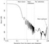 |
Fig. 1 Example of a cut of the simulated beam pattern of the 70GHz LFI18-S radiometer. The cut passes through the main reflector spillover of the Planck telescope. The plot shows, in particular, the level and shape of the near sidelobes. |
2.1.3. Polarization angle
We now discuss the systematic effect caused by the uncertainty in the orientation of the feedhorns in the focal plane. From thermo-elastic simulations, we found this uncertainty to be about 0.2° (Villa et al. 2005). In this study we adopt a more conservative approach in which we set the uncertainties using measurements of the Crab Nebula. Then we performed a sensitivity study in which we considered a fiducial sky observed with a certain polarization angle for each feedhorn and then reconstructed the sky with a slightly different polarization angle for each feedhorn. The differences span the range of uncertainties in the polarization angle derived from measurements of the Crab Nebula.
In this section we first recall our definition of polarization angle and then discuss the rationale we used to define the “error bars” in our sensitivity study.
Definition of polarization angle.
Each LFI scanning beam6 is defined in a reference frame specified by the three angles θuv, φuv, and ψuv, reported in Table 5 of Planck Collaboration II (2016) and shown in Fig. 2. This choice implies that the power peak of the co-polar component lies along the main beam pointing direction, and a minimum in the cross-polar component appears in the same direction (Planck Collaboration IV 2016). In particular, the major axis of the polarization ellipse is along the x-axis for the radiometer side arm (S), and it is aligned with the y-axis for the radiometer main arm (M).
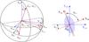 |
Fig. 2 Definition of polarization angle. Left: the orientation of the main beam frame, (XYZ)MB, with respect to the line-of-sight (LOS) frame, (XYZ)LOS, is defined by the three angles θuv, φuv, and ψuv. The intermediate frame, (XYZ)DX, is the detector frame, defined by the two angles θuv and φuv. Right: the angle ψpol is defined with respect to XMB and represents the orientation of the polarization ellipse along the beam line of sight. It is very close to 0 or 90 deg for the S and M radiometers, respectively. |
The main beam is essentially linearly polarized in directions close to the beam pointing. The x-axis of the main beam frame can be assumed to be the main beam polarization direction for the S radiometers, and the y-axis of the main beam frame can be assumed to be the main beam polarization direction for the M radiometers.
We define ψpol as the angle between the main beam polarization direction and the x-axis of the main beam frame, and define the main beam polarization angle, ψ, as ψ = ψuv + ψpol. The angle ψpol is nominally either 0° or 90° for the side and main arms, respectively.
The values of ψpol can be either determined from measured data using the Crab Nebula as a calibrator, or from optical simulations performed coupling the LFI feedhorns to the Planck telescope, considering both the optical and radiometer bandpass responses7.
For the current release our analysis uses values of ψpol derived from simulations. Indeed, the optical model is constrained well by the main beam reconstruction carried out with seven Jupiter transits and provides us with more accurate estimates of the polarization angle compared to direct measurements.
As an independent crosscheck, we also consider our measurements of the Crab Nebula as a polarized calibrating source. We use a least-squares fit of the time-ordered data measured during Crab scans to determine I, Q, and U and, consequently, the polarization angle. Then we incorporate the instrument noise via the covariance matrix and obtain the final error bars by adding the uncertainties due to the bandpass mismatch correction in quadrature (Planck Collaboration II 2016).
While such a check is desirable, we find that the polarization angles derived from these data display systematic errors that are much larger than those expected from our noise and bandpass mismatch correction alone, especially at 30 and 44GHz (horns from LFI24 through LFI28; see Fig. 3). In particular, we find that the values obtained for the various horns in the focal plane display differences that are larger than our error estimates.
The horn with the largest apparent offset in angle, LFI25, is the solitary 44GHz horn on one side of the focal plane; in the next data release, we will examine this discrepancy in more detail.
An important difficulty is to determine the relative gains of the individually polarized receivers, particularly during the Crab crossings, which appear near the minima of our main temperature calibration. Another souce of uncertainty missing from the Crab analysis is beam errors. Of course, the LFI radiometer polarization angles do not change over time, but the variability in the estimates limits our use of the Crab crossings for this purpose.
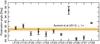 |
Fig. 3 Crab Nebula polarization angle measured by the various feedhorns in the focal plane. The straight horizontal line reports the value from Aumont et al. (2010) converted to Galactic coordinates, and the yellow area is the ± 1σ uncertainty. |
Definition of error bars.
The ψpol angle can differ from its nominal value because of small misalignments induced by the mechanical tolerances, thermo-mechanical effects during cooldown, and by uncertainties in the the optical and radiometer behaviour across the band. If we consider the variation of ψpol across the band in our simulations, for example, we find deviations from the nominal values that are, at most, 0.5°.
To estimate the impact of imperfect knowledge of the polarization angle on CMB maps, we use the errors derived in the Crab analysis, which include the scan strategy, white noise and bandpass mismatch-correction errors. While the errors derived this way are not designed to capture the time variation of the actual Crab measurements, we believe they provide a conservative upper bound to the errors in our knowledge of the instrument polarization angles.
The two panels in Fig. 4 show the values of ψpol derived from GRASP simulations (which are also used by the data analysis pipeline) and the error bars obtained from Crab observations. We notice that the scatter of the simulated angles is much less than the size of the error bars. This is consistent with uncertainty on the simulated angles that is much smaller than the error bars derived from Crab measurements. These data are the basis of the simulation exercise discussed in Sect. 3.2.1.
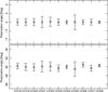 |
Fig. 4 Simulated polarization angles and error bars from the Crab measurements used in the analysis. Top: radiometer main arm. Bottom: radiometer side arm. The scatter of the plotted angles is much less than the error bars because the uncertainty in our simulations is much smaller than the error bars derived from Crab measurements. |
Our on-ground determination of radiometer polarization angles is more than sufficient for the CMB polarization. As seen in the measurements of the Crab Nebula, the impact of gain errors among our polarized radiometers may be important, and we do include this effect in our gain error simulations.
2.1.4. Pointing
Pointing reconstruction is performed in two steps. The first is to reconstruct the satellite attitude, and the second is to measure the orientation of the individual detectors with respect to the focal plane boresight (focal plane geometry reconstruction). In the first step we take all common-mode variations into account between the star camera and focal plane frames and assume the focal plane reconstruction, so that the focal plane geometry is essentially fixed over the entire mission.
Planet scans indicate that the satellite attitude, reconstructed from the star camera data, contains slow timescale variations (≳1month) leading to total errors up to about 30′′. The two major modes are a linear drift and a modulation that is heavily correlated with the Sun-Earth distance. To correct these fluctuations, we fit a linear drift and a solar distance template to the planet position offsets and include discontinuous steps at known disturbances of the thermal environment. More details about the pointing reconstruction can be found in Sect. 5.3 of Planck Collaboration I (2016).
In this paper we evaluate the impact on the CMB maps and power spectra of residual uncertainties in the pointing reconstruction process. We performed the assessment using simulations in which the same sky is observed with two different pointing solutions that represent the uncertainty upper limit. We describe the approach and the results obtained in Sect. 3.2.1.
2.2. Imperfect calibration
The analysis of the first data release showed that the uncertainty in the calibration is one of the main factors driving the systematic effects budget for Planck-LFI. The accuracy of the retrieved calibration constant depends on the signal-to-noise ratio (S/N) between the dipole and instrumental noise along the scan directions, on effects causing gain variations (e.g., focal plane temperature fluctuations), and on the presence of Galactic straylight in the measured signal.
In the analysis for the 2015 release, we have substantially revised our calibration pipeline to account for these effects and to improve the accuracy of the calibration. The full details are provided in Planck Collaboration V (2016), and here we briefly list the most important changes: (i) we derive the solar dipole parameters using LFI-only data, so that we no longer rely on parameters provided by Hinshaw et al. (2009); (ii) we take the shape of the beams over the full 4π sphere into account; (iii) we use an improved iterative calibration algorithm to estimate the calibration constant K (measured in VK-1)8; and (iv) we use a new smoothing algorithm to reduce the statistical uncertainty in the estimates of K and to account for gain changes caused by variations in the instrument environment.
We nevertheless expect residual systematic effects in the calibration constants due to uncertainties in the following pipeline steps.
- 1.
Solar dipole parameters derived from LFI data. This only affects the absolute calibration and the overall dynamic range of the maps, as well as the power spectrum level. We discuss the absolute calibration accuracy in Planck Collaboration V (2016) and do not address it further here.
- 2.
Optical model and radiometer bandpass response. This enters the computation of the 4π beams, which are used to account for Galactic straylight in the calibration.
- 3.
A number of effects (e.g., the impact of residual Galactic foregrounds) that might bias the estimates of the calibration constant K.
- 4.
The smoothing filter we use to reduce the scatter in the values of K near periods of dipole minima. This filter might be too aggressive, removing features from the set of K measurements that are not due to noise. This could cause systematic errors in the temperature and polarization data.
We are currently evaluating ways to improve this assessment in the context of the next Planck release. One possibility would be to use Monte Carlo simulations to assess the impact on calibration of uncertainties in the beam far sidelobes.
2.3. Bandpass mismatch
Mismatch between the bandpasses of the two orthogonally-polarized arms of the LFI radiometers causes leakage of foreground total intensity into the polarization maps. The effect and our correction for it are described in Sect. 11 of Planck Collaboration II (2016) and references therein. A point to note is that the correction is only applied to at an angular resolution of 1°, although Appendix C of Planck Collaboration XXVI (2016) describes a special procedure for correcting point source photometry derived from the full resolution maps.
Residual discrepancies between the blind and model-driven estimates of the leakage are noted in Planck Collaboration II (2016), which imply that the small (typically <1%) mismatch corrections are not perfect. The estimated fractional uncertainty in these corrections is <25% at 70GHz and <3% at 30GHz; the discrepancies are significant only because they are driven by the intense foreground emission on the Galactic plane.
List of the simulated systematic effects.
As explained in Sect. 3.1, our cosmological analysis of polarization data is restricted to 46% of the sky with the weakest foreground emission. Planck Collaboration XI (2016) demonstrates that in this region the bandpass correction has a negligible effect on the angular power spectrum and cosmological parameters derived from it, the optical depth to reionization, τ, and the power spectrum amplitude. The same applies to our upper limit on the tensor-to-scalar ratio, Consequently the impact of the uncertainty in the correction is also negligible for the cosmological results.
3. Assessing residual systematic effect uncertainties in maps and power spectra
In this section we describe our assessment of systematic effects in the LFI data, which is based on a two-steps approach.
The first is to simulate maps of each effect (see Table 2) and combine them into a global map that contains the sum of all the effects. We perform simulations for various time intervals, single surveys, individual years, and full mission, and we use such simulations to produce a set of difference maps. For example, we construct year-difference maps of global systematic effects as the sum of all the effects for one year subtracted from the sum of all effects from another year. We also compare the pseudo-spectra computed on the full-mission maps with the expected sky signal to assess the impact of the various effects. This step is described in Sect. 3.2.
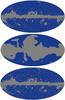 |
Fig. 5 Masks used in this work. Top: mask used to compute power spectra of simulated systematic effect total intensity maps. Middle: mask used to compute power spectra of Q and U systematic-effect maps. Bottom: mask used to compute power spectra of null maps. |
The second is to calculate the same difference maps from flight data. We call these maps null maps, because they should contain only white noise, as the sky observed in the time intervals of each pair of maps is the same. Here we compare the null maps pseudo-spectra with the pseudo-spectra of the global systematic effects difference maps. Our objective, in this case, is to highlight any residuals in the pseudo-spectra obtained from flight data that are not accounted for by our simulations. This step is described in Sect. 3.3.
In all cases we compute pseudo-spectra using the HEALPix anafast code and correct for the fraction of observed sky. In other words, in all the power spectra of this work we have Cℓ = Cℓ,anafast/fsky, where Cℓ,anafast is the power spectrum as obtained by the anafast code and fsky is the fraction of observed sky.
3.1. Masks
We start by reviewing the masks applied in the calculation of the pseudo-spectra used in our assessment. We have used three masks to compute the power spectra discussed in this paper , and we show them in the three panels of Fig. 5.
The first mask (top panel of Fig. 5) is used for total intensity maps of the systematic effects. It removes the Galactic plane and point sources. It is the “UT78” mask described in Sect. 4.1 of Planck Collaboration IX (2016), obtained by combining the Commander, SEVEM, and SMICA confidence masks.
The second mask (middle panel of Fig. 5) is used for Q and U maps of the systematic effects. It removes about 54% of the sky, cutting out a large portion of the Galactic plane and the Northern and Southern Spurs. We adopted this mask in the low-ℓ likelihood used to extract the reionization optical depth parameter, τ (see Fig. 3 in Planck Collaboration XI 2016). We chose to use the same mask in the assessment of systematic effect uncertainties in polarization.
The third mask (bottom panel of Fig. 5) is used in the null-map analysis at all frequencies both in temperature and polarization. We obtained this mask by combining the UPB77 30-GHz polarization mask (right panel of Fig. 1 in Planck Collaboration IX 2016) and the 30-GHz point source mask used for the 2013 release described in Sect. 4 of Planck Collaboration XII (2014)9.
3.2. Assessing systematic effects via simulations (“bottom-up”)
3.2.1. Optics and pointing
Far and near sidelobes.
To assess the effect of far and near sidelobes we simulate the residual signal by observing a fiducial sky with a beam pattern that only contains the beam component being tested. The sky signal contains the CMB and foregrounds as observed by each radiometer, including the spurious polarization caused by the bandpass mismatch. Further details regarding the the fiducial sky can be found in Planck Collaboration XII (2016), a description of the simulation pipeline is in Reinecke et al. (2006), and the Madam mapmaker is described in Kurki-Suonio et al. (2009) and Keihänen et al. (2010).
We perform this assessment by projecting timelines of the sky convolved with the beam pattern into maps. First we use the spherical harmonic components of the beam (Planck Collaboration IV 2016) to generate timelines10. Then we produce maps using the Madam mapmaker with the same parameters used for the sky maps (Planck Collaboration VI 2016).
We simulate far sidelobes with the GRASP Mr-GTD11 analysis, considering all the first-order contributions and two contributions at second order (reflections and diffractions from the sub-reflector, which are diffracted by the main reflector). This choice allows us to keep the computational time within the available CPU resources at the cost of a small fraction of power that is not accounted for in the sidelobe region of the beam pattern.
The power lost because of our approximation is ≲0.5% (see Table 1 in Planck Collaboration IV 2016). To estimate the level of uncertainty introduced by this lost power, we rescale the far-sidelobe spherical harmonic coefficients so that the total beam efficiency is equal to 100%. Then we simulate maps of the effect from native and rescaled sidelobes and compare the two corresponding power spectra.
Figure 6 shows the impact of this approximation. The coloured area is the region in ℓ space between the two power spectra, and represents the uncertainty due to the first-order approximation in the GRASP analysis. For the purpose of comparing the power spectrum of systematic effects with the sky signal, this uncertainty is small so we have neglected it.
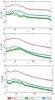 |
Fig. 6 Uncertainty in the power spectra of the effect from far sidelobes introduced by the first-order approximation in GRASP simulations. Top: TT spectrum. Middle: EE spectrum. Bottom: BB spectrum. For each frequency the coloured area is the region between the native power spectrum and the one rescaled to account for the missing power. |
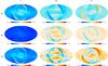 |
Fig. 7 Maps of the effect from far sidelobes. Rows correspond to 30, 44, and 70GHz channels, while columns correspond to I, Q, and U. The straylight signal at 30GHz is larger compared to 44 and 70GHz. The 44GHz channel is the least contaminated by this effect. This behaviour results from the combination of the beam far sidelobes and the intensity of the Galactic emissions at the LFI frequencies. |
Figure 7 shows full-sky maps of the Galactic straylight detected by the far-sidelobe beam patterns. This signal is removed from the timelines, so we do not consider it in the budget of systematic uncertainties. Moreover, in Figs. 24−26, we plot the power spectrum of this effect and show that even if we did not remove it from the data, the effect would be at a level much lower than the sky signal.
Our results show that the effect from Galactic straylight is significantly more at 30GHz compared to 44 and 70GHz, for which the level of the spurious signal is similar.
To understand this result one must consider that this effect depends on two factors: (i) the level of the beam far sidelobes and (ii) the intensity of the Galactic signal. The level of the beam far sidelobes results from the coupling of the feed-horn beam pattern with the secondary mirror.
A larger feed-horn main beam illuminates the secondary mirror more effectively. This determines a narrower main beam of the entire optical system and a higher level of far sidelobes. In Planck-LFI the 44GHz feedhorns have narrower beams than do the 30 and 70GHz horns, and for this reason, the power in the far sidelobes is significantly smaller.
If we also consider that the Galactic signal intensity decreases with frequency, we understand our result, which is completely consistent with pre-launch optical simulations. The interested reader can find more details in Sandri et al. (2004, 2010) and Burigana et al. (2004).
Ideally our analysis would assess the impact of the accuracy in our far-sidelobe model on the systematic effects analysis. The proper way to do this would be to identify the sources of uncertainty in the model and run Monte Carlo simulations, producing several far sidelobes with GRASP and propagating the analysis to sky maps and power spectra.
This analysis would require a considerable amount of computing time, and we did not perform it for this release, but instead rely on null-test analyses. Null maps from consecutive surveys are quite sensitive to the pickup of straylight by the far sidelobes and can be used to assess the presence of straylight residuals in the data. We discuss this point in Sect. 3.3.
We study the effect coming from the near sidelobes following the same procedure used for the far sidelobes. The main difference is that, in this case, we did not apply any correction to the data, so that our simulations estimate the systematic effect that we expect to be present in the data.
The maps in Fig. 8 show that near sidelobes especially impact measurements close to the Galactic plane. This is expected, because this region of the beam pattern is close to the main beam and causes a spurious signal when the beam scans regions of the sky with large brightness variations on small angular scales. This implies that near sidelobes do not significantly affect the recovery of the CMB power spectrum if the Galactic plane is properly masked. We confirm this through the power spectra, as shown in Figs. 24−26.
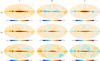 |
Fig. 8 Maps of the effect from near sidelobes. Rows correspond to 30, 44, and 70GHz channels, while columns correspond to I, Q, and U. |
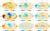 |
Fig. 9 Maps of the effect from uncertainty in the polarization angle. The maps shown are randomly selected from one of the five tested realizations. Rows correspond to 30, 44, and 70GHz channels, while columns correspond to I, Q, and U. |
Polarization angle.
We study how the uncertainty in the polarization angle affects the recovered power spectra by means of a limited Monte Carlo exercise. We first produced a fiducial sky containing the CMB and foregrounds observed with the nominal polarization angles (Fig. 4), and then we generated five additional skies observed with a slightly different polarization angle for each feedhorn. Finally we computed the difference between each of the five maps and the fiducial sky.
In each of the five cases we rotated the polarization angle of each feedhorn by an amount equal to either the maximum or the minimum of the error bars shown in Fig. 4. In this way we could explore, for a small number of cases, a range of variability in the polarization angle that is greater than the range expected from the focal plane thermo-mechanical analysis.
The difference maps in Fig. 9 show that the effect is negligible in temperature (as expected) and is less than 1μK at 70GHz in polarization. At 30 and 44GHz the maximum amplitude of the effect is around 2μK and 1μK, respectively. The maps shown represent one of the five cases picked randomly from the set.
In Figs. 10 and 11 we show the dispersion of the peak-to-peak and rms of this effect on maps, once we apply the masks in Fig. 5 (top one for total intensity and middle one for Q and U maps). The rms of the effect is smaller than 1μK, and the dispersion introduced by the five different cases is also small.
We observe that the peak-to-peak and rms of the effect in the polarization map decrease with frequency (see the bottom panels of Figs. 10 and 11). This correlates with the smaller contribution of polarized synchrotron emission in maps at higher frequency.
We also observe a higher residual at 44GHz in temperature maps compared to the 30 and 70GHz channels. We did not expect this behaviour, and it is currently not understood. The effect in temperature, however, is much less than 0.1μK and, therefore, completely negligible.
From the five sets of difference maps, we computed power spectra and evaluated their dispersion. We show the results in Fig. 12 with the region containing all the spectra and the average of these five spectra. The blue curve corresponds to the spectrum that is also reported in Figs. 24−26.
Pointing.
We simulated the effect caused by pointing uncertainty by adding a Gaussian noise realization independently to both co-scan and cross-scan bore sight pointings. The noise realization was drawn from a 1 /f noise model with a smooth cutoff at 10mHz, which matches the single-planet transit analysis and multiple transit results over the entire mission. The rms net effect of the added pointing errors is an uncertainty of about 4.8′′ on timescales shorter than 10000s, and about 5.1′′ on timescales longer than 10000s. The overall uncertainty is approximately 7.0′′.
Figure 13 shows full-sky maps of the estimated systematic effect caused by pointing uncertainty.
The level of the spurious residual is very low. In polarization it is much less than 1μK at all frequencies, whereas in total intensity it is higher, a few μK, since it is dominated by point sources along the Galactic plane. The 30GHz channel is the most affected by this effect; this is expected, because at 30GHz the emission from point sources is stronger than at higher frequencies, and the reconstruction of their positions on the sky is particularly sensitive to pointing accuracy.
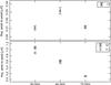 |
Fig. 10 Peak-to-peak value of the effect from polarization angle uncertainty on LFI maps. The error bars represent the dispersion of the five cases chosen in the analysis. Top: total intensity. Bottom: Q and U Stokes parameters. |
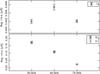 |
Fig. 11 Rms of the effect from polarization angle uncertainty on LFI maps. The error bars represent the dispersion of the five cases chosen in the analysis. Top: total intensity. Bottom: Q and U Stokes parameters. |
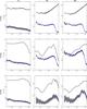 |
Fig. 12 Angular power spectra of the residual effect of polarization angle uncertainty compared to the foreground spectra at 30GHz and to Planck beam-filtered temperature and polarization spectra at 44 and 70GHz. The blue curve represents the average spectrum, while the grey band is the envelope of all the power spectra calculated from the various realizations of the effect. The theoretical B-mode CMB spectrum assumes a tensor-to-scalar ratio r = 0.1, a tensor spectral index nT = 0 and has not been beam-filtered. Rows are for 30, 44, and 70GHz spectra, while columns are for TT, EE, and BB power spectra. |
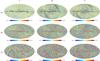 |
Fig. 13 Maps of the effect of pointing errors. Rows correspond to 30, 44, and 70GHz channels, while columns correspond to I, Q, and U. |
3.2.2. Imperfect calibration
We assess the effect of uncertainties in the relative photometric calibration of each radiometer by differencing a model sky map and a second map obtained by applying the same calibration pipeline used in the data analysis.
We start by generating timelines from the measured sky maps at 30, 44, and 70GHz. We use these maps as our model sky, which was already convolved with the telescope beam pattern and radiometric bandpass response. These maps contain the CMB, the diffuse foreground emission, and a small residual of the instrument noise and systematic effects. We are interested in how well the calibration pipeline is able to reproduce this model sky, so that these residuals do not represent a limitation in our analysis.
Then we add the following three components: (i) the dipole signal convolved with the model sidelobes (see Sect. 7.1 of Planck Collaboration II 2016); (ii) the Galactic straylight estimated according to the procedure described in Sect. 7.4 of Planck Collaboration II (2016); and (iii) the radiometer noise (white +1 /f) generated starting from the radiometer parameters in the instrument database. We report and discuss these parameters in Table 10 of Planck Collaboration II (2016).
The final step in data preparation is to convert the timelines into voltage units. We do this by multiplying each sample by the corresponding gain constant used in the data analysis. We chose this approach to have a variability that closely represents the actual measurements. We also repeated this exercise with different choices of the fiducial gain solution and verified that the result does not depend on them at first order.
At this point we apply the calibration pipeline to these timelines to recover the gain constants. These constants will not be identical to the input ones, because of the noise present in the data. The combination of the dipole and Galactic straylight variability with the instrument noise causes a difference between the input and recovered constants that varies with time.
We evaluate the impact of the difference between the input and recovered gain constants by differencing the input maps with those generate using the recovered gains. We show these maps in Fig. 14. These maps show that the effect is of the order of 2μK peak-to-peak at 44 and 70GHz, and 6μK peak-to-peak at 30GHz.
This is the effect with the largest impact on LFI polarization data and drives the systematic effect uncertainties. At 30GHz the residual is about five orders of magnitudes less than the synchrotron emission in temperature and about ten times less in polarization. We expect, therefore, that we can use this channel as a foreground template with negligible impact from systematic uncertainties. We have verified this in the analysis presented in Sect. 3.4, where we assess the impact of systematic effects in the 30 and 70GHz channels on the reionization optical depth parameter, τ.
At 70GHz the residual is less than the CMB E-mode power spectrum, apart from the range of multipoles 10–20. We evaluated the impact of these uncertainties on the reionization optical depth, τ, and found them to be small. We discuss this assessment in Sect. 3.4. At 44GHz the residual effect is at the level of the E-mode power spectrum for ℓ< 10 and exceeds it in the multipoles range 10–30. In this release we did not use the 44GHz data in the extraction of τ. We are currently evaluating strategies to improve the photometric calibration accuracy and will report the results of this effort in the context of the next release.
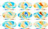 |
Fig. 14 Maps of the effect from imperfect relative calibration. Rows correspond to 30, 44, and 70GHz channels, while columns correspond to I, Q, and U. Maps are smoothed to the beam optical resolution of each channel (θFWHM = 33′, 28′, and 13′, respectively). |
3.2.3. ADC nonlinearity
We assess the effect of the ADC nonlinearity by taking differences between simulated maps containing the ADC effect and fiducial, clean maps. This is the same approach as described in Planck Collaboration III (2014), and it is based on the following steps.
First, we produce time-ordered data with and without a known ADC error for each detector. To do this we start from full-mission sky maps and rescan them into time-ordered data using the pointing information. We de-calibrate the data using a gain model based on the actual average of the calibration constant and time variations obtained from relative fluctuations of the reference voltage (the “4-K calibration” method described in Sect. 3 of Planck Collaboration V 2014). Then we add voltage offsets, drifts, and noise, in agreement with those observed in the real, raw data.
We add the ADC effect to the time-ordered data of each detector by applying the inverse spline curve used to correct the data. For the channels where we do not apply any correction we add a conservative estimate of the effect using the estimator ϵADC = (1 / ⟨ Vsky ⟩ )(δVWN,sky/δVWN,ref), where ⟨ Vsky ⟩ is the average sky voltage and δVWN,sky, δVWN,ref are the estimates of the white noise in the sky and reference load voltages, respectively. We discuss the rationale behind this choice in Appendix B of Planck Collaboration III (2014).
We then determine ADC correction curves from these simulated time-ordered data and remove the estimated effect. A residual remains, though, since the reconstruction is not perfect because of the presence of noise in the data. The effect of this residual is what we estimate in our simulations.
Finally we produce difference maps from time-ordered data with and without the residual ADC effect (Fig. 15). In our previous results (Planck Collaboration III 2014) the rms fluctuations away from the Galactic plane were about 1 and 0.3μK at 30 and 44GHz. Now they are 0.3 and 0.1μK, respectively. In these two frequency channels Q and U maps show ADC stripes at the level of 0.07 and 0.05μK, respectively. In the Galactic plane we see features in both intensity and polarization at the level of a few μK at 30GHz and a fraction of a μK at 44GHz.
The case at 70GHz is more complicated, because the white noise is higher and also because the data from some of the diodes were not corrected. This leads to the appearance of a broad stripe with an amplitude of about 0.3μK.
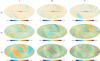 |
Fig. 15 Maps of the ADC nonlinearity effect. Rows correspond to 30, 44, and 70GHz channels, while columns correspond to I, Q, and U. Maps are smoothed to the beam optical resolution of each channel (θFWHM = 33′, 28′, and 13′, respectively). |
3.2.4. Thermal effects
Temperature fluctuations of the 4-K reference loads, of the 20-K focal plane, and of the 300-K receiver back-end modules are a source of systematic variations in the measured signal. Fluctuations in the temperature of the 4-K reference loads couple directly with the differential measurements, while fluctuations in the 20-K and 300-K stages couple with the detected signal through thermal and radiometric transfer functions. Thermal transfer functions are described in Sect. 3 of Tomasi et al. (2010), while a complete description of the radiometric coupling with temperature fluctuations can be found in Terenzi et al. (2009). We also provide a general treatment of the susceptibility of the LFI receivers to systematic effects in Sect. 3 of Seiffert et al. (2002, see, especially, Eq. (10)).
The three panels in Fig. 16 show the behaviour of the relevant LFI temperature over the entire mission, with labels identifying relevant events that occurred during the mission. The grey bands identify the eight surveys.
The top panel shows the temperature of the 4-K loads at the level of the 30 and 44GHz (bottom curve) and 70GHz (top curve) channels. The rms variation of this temperature over the whole mission is σ30,44 = 1.55mK and σ70 = 80μK.
The middle panel displays the 20-K focal plane temperature measured by a sensor mounted on the flange of the 30GHz LFI28 receiver feedhorn. There are some notable features. The most stable period is the one corresponding to the first survey. After the sorption cooler switchover we see a period of temperature instability that spanned about half of the third survey and that was later controlled by commanded temperature steps that we continued to apply until the end of the mission. The bottom panel shows the behaviour of one of the the back-end temperature sensors. We notice a short-period temperature fluctuation during the first survey, which was caused by the daily on-off switching of the transponder. This was later left on to reduce these 24-h variations (see the temperature increase after day 200). We also see a temperature drop corresponding to the sorption cooler switchover and a seasonal periodic variation correlated with the yearly orbit around the Sun.
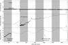 |
Fig. 16 Top: temperature measured by two sensors mounted on the HFI 4-K shield at the level of 30 and 44GHz (bottom curve) and 70GHz (top curve) reference loads. The rms variation of this temperature over the full mission is σ30,44 = 1.55mK and σ70 = 80μK. Middle: temperature of the 20-K focal plane measured by a temperature sensor placed on the flange of the LFI28 30GHz feedhorn. The consecutive temperature steps after day 500 reflect changes to the set point of the temperature control system. We applied these changes to control the level of temperature fluctuations. Bottom: temperature of the 300-K back-end unit. |
We assessed the effect of temperature variations following the procedure described in Sect. 4.2.1 of Planck Collaboration III (2014). We combined temperature measurements with thermal and radiometric transfer functions to obtain time-ordered data of the systematic effects. We then used these time-ordered data and pointing information to produce maps. For this release we used the same thermal and radiometric transfer functions that were applied analysing the 2013 release.
In Fig. 17 we show maps in total intensity and polarization of the combined thermal effects. In each of these maps the impact of thermal fluctuations is less than 1μK, which is negligible.
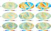 |
Fig. 17 Maps of thermal systematic effects. Rows correspond to 30, 44, and 70GHz channels, while columns correspond to I, Q, and U. Maps are smoothed to the beam optical resolution of each channel (θFWHM = 33′, 28′, and 13′, respectively). |
3.2.5. Bias fluctuations
We assess the effect of bias fluctuations in the LFI front-end modules on temperature and polarization measurements, disentangling the various sources of electrical instabilities. They are:
-
thermal fluctuations in the analog electronics;
-
thermal fluctuations in the instrument front-end;
-
electrical instabilities in analogue electronics; and
-
electrical instabilities affecting the cold amplifiers that may be generated either inside or outside the device (e.g., electric line instabilities or cosmic rays).
We follow a procedure in which we correlate the radiometric signal with measured drain currents. For each radiometer we first remove fluctuations caused by thermal instabilities in the cold and warm units (Eq. (1) in Planck Collaboration III 2014), and then we correlate the residual drain current fluctuations with the voltage output of both radiometer diodes (Eq. (2) in Planck Collaboration III 2014).
We obtain four coefficients: two of them (α20K and α300K) are the correlation coefficients between the measured currents and temperatures, and the other two (αsky and αref) link the total power sky and reference-load voltage outputs with drain current measurements corrected for thermal effects.
In this release we updated αsky and αref, exploiting the possibility of measuring drain currents every 6s instead of every 64s (the default time interval for this housekeeping parameter). To enable this faster acquisition, we developed a dedicated telemetry procedure that was not available for the 2013 release.
The thermal coefficients, instead, are the same as those used in the 2013 release. We measured them by exploiting controlled temperature variations during the in-flight calibration phase (Gregorio et al. 2013) and temperature fluctuations induced by the transponder being switched on and off every day during the first survey (see Fig. 26 in Planck Collaboration II 2011). Since we did not perform other tests involving temperature changes during the mission we did not update α20K and α300K between the 2013 and 2015 data release.
With these coefficients we used the drain current measurements to generate time-ordered data that we projected onto the sky.
Figure 18 shows maps in temperature and polarization of the systematic effect from bias fluctuations. This effect is less than 1μK both in temperature and polarization, which is negligible compared to the CMB at 44 and 70GHz and foregrounds at 30GHz. These results are also consistent with the 2013 analysis in temperature (Planck Collaboration III 2014).
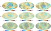 |
Fig. 18 Maps of the effect from front-end bias fluctuations. Rows correspond to 30, 44, and 70GHz channels, while columns correspond to I, Q, and U. Maps are smoothed to the beam optical resolution of each channel (θFWHM = 33′, 28′, and 13′, respectively). |
3.2.6. 1-Hz spikes
This effect is caused by a well-known cross-talk between the housekeeping 1-Hz acquisition clock and the scientific data acquisition. We have described this effect in several previous papers. In Sect. 5.2.5 of Mennella et al. (2010), we discussed how we characterized it during ground tests; in Sect. 4.1.2 of Gregorio et al. (2013) we presented a similar characterization performed during flight calibration, in Sect. 3.1 of Zacchei et al. (2011), we explained how we build templates of this effect and remove them from the data; and in Sect. 4.2.3 of Planck Collaboration III (2014), we show how we assess the impact of residual uncertainties on the LFI CMB temperature results.
Here we extend our analysis to temperature and polarization data using the full mission data set with the same procedure as explained in Planck Collaboration III (2014).
The maps in Fig. 19 show that this effect is less than 1μK at 30 and 70GHz and about 1–2μK at 44GHz. This channel is indeed the most affected by 1-Hz spikes, and it is the only one that we correct by removing the signal template from the time-ordered data. The 30 and 70GHz data, instead, are only slightly affected by this spurious signal so we have not applied any correction.
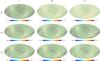 |
Fig. 19 Maps of the effect from 1-Hz spikes. Rows correspond to 30, 44, and 70GHz channels, while columns correspond to I, Q, and U. Maps are smoothed to the beam optical resolution of each channel (θFWHM = 33′, 28′, and 13′, respectively). |
3.3. Assessing systematic effects via null tests (“top-down”)
We define “null test” as an analysis based on differences between subsets of data (maps, timelines, power spectra, etc.) that, in principle, contain the same sky signal. The Planck scanning strategy (see Sect. 4.1 of Planck Collaboration I 2016), together with the symmetric configuration of the focal plane (see Fig. 11 of Bersanelli et al. 2010, and Fig. 4 of Lamarre et al. 2010), offers several useful null-test combinations, each with a different sensitivity to various kinds of systematic effects in both temperature and in polarization.
We have routinely carried out null tests during the LFI data analysis. These tests played a key role in our understanding of the LFI systematic error budget, and led to improvements in the self-consistency of our data. These improvements have allowed us to use the LFI polarization results on the largest angular scales.
In this section we discuss the results of our null test analysis. First we discuss the general strategy and then we present the results obtained showing the robustness of the LFI data against several classes of systematic effects.
3.3.1. Null-test strategy
We complement each Planck-LFI data release with a suite of null tests that combine data selected at various timescales.
The shortest timescale is that of a single pointing period (~40 min) that is split into two parts. We then difference the corresponding maps and obtain the so-called half-ring difference maps that approximate the instrument noise and may contain systematic effects correlated on timescales ≲20 min.
Then we have longer timescales: six months (a sky survey), one year, the full mission (four years). We can create a large number of tests by combining these timescales for single radiometers12. We provide the detailed timing of each survey in the Planck Explanatory Supplement13.
When we take a difference between two maps we apply a weighting to guarantee that we obtain the same level of white noise independently of the timescale considered. The weighting scheme is described by Eqs. (30)−(32) of Planck Collaboration II (2011), where we normalize the white noise to the full mission (8 surveys) noise. This means that in Eq. (32) of Planck Collaboration II (2011), the term hitfull(p) corresponds to the number of hits at each pixel, p, in the full map.
We assess the quality of the null tests by comparing null-map pseudo spectra obtained from flight data with those coming from systematic effect simulations and with noise-only Monte Carlo realizations based on the Planckfull focal plane (FFP8) simulation (Planck Collaboration XII 2016). For the systematic effect simulations, we used global maps by combining the effects listed in Table 2. Monte Carlo realizations include pointing, flagging, and a radiometer specific noise model based on the measured noise power spectrum. We create 1000 random realizations of such noise maps using the same destriping algorithm as used for the real data, and compute null maps and pseudo-spectra in the same way. For each multipole, ℓ, we calculate the mean Cℓ and its dispersion by fitting the 1000 Cℓs with an asymmetric Gaussian.
Passing these null tests is a strong indication of self-consistency. Of course, some effects could be present, at a certain level, on the various timescales, so that they are canceled out in the difference and remain undetected. However, the combined set of map differences allows us to gain confidence in our data and noise model.
In the following part of this section we present the results of some null test analyses, that highlight the data consistency with respect to various classes of systematic effects. All the power spectra are pseudo-spectra computed on maps masked with the bottom mask shown in Fig. 5.
Our results show the level of consistency of the LFI data. At 70GHz, in particular, the data pass all our tests both in temperature and polarization. Small residuals exist at lower frequencies, especially at 30GHz. At this frequency we see the evidence of residuals probably due to an imperfect Galactic straylight removal from our data (see results in Sect. 3.3.4).
None of the detected excess cases appear to be crucial for science analysis. Residuals in temperature (which are expected to be larger due to the much stronger sky signals) are still orders of magnitude below the power of the signal from the sky (see left-hand panels of Figs. 24−26). We use the 30GHz channel in polarization (middle and right-hand panels of Fig. 24) as a synchrotron monitor for the Planck CMB channels, and the observed deviations are small for foreground analysis or component separation.
3.3.2. Highlighting residuals in subsets of data with “full−year” difference maps
We check the consistency of data acquired during each year using the full-mission map of the corresponding frequency as a reference to identify particular years that appear anomalous compared to others. For example, we tested for spurious residuals in the first year of data of the 70GHz channel by taking the difference between the year-1 and full-mission maps at 70GHz.
The full-mission maps may contain some residual systematic effects, but this is not a problem in the context of this test, which aims at highlighting relative differences among the various year-long datasets. Furthermore, systematic effects average out more efficiently in full-mission maps than in single-year or single-survey maps. We verified this by calculating the peak-to-peak variations in simulated maps containing the sum of all systematic effects. Then we took the ratio between this peak-to-peak value calculated for year-maps and the value for full-mission maps and obtained values that from 1.2 at 30GHz to 2.1 at 70GHz.
In Fig. 20 we show the results of pseudo spectra from full−year difference maps obtained from data and simulations compared to the range of spectra obtained from the 1000 noise-only Monte Carlo simulations. This range is indicated by the coloured area, which represents the rms spread of the simulated spectra.
Our analysis shows that at 44 and 70GHz the null power spectra are explained by noise, while at 30GHz there are some residuals slightly exceeding the 1σ region of the Monte Carlo simulations. The null spectra from simulated systematic effects are below the noise level apart from the first multipoles where the simulations in some cases reach the noise level.
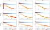 |
Fig. 20 Angular power spectra of full−year maps. Coloured lines represent the four nulls obtained from data and simulations of the effects listed in Table 2. The purple area represents the envelope from Monte Carlo simulations as described in the text. In this figure we can appreciate that the power spectra of the data from the null maps are well matched by noise, except for a few low-ℓ points at 30GHz. Furthermore, the power spectra of the simulated systematic effects fall well below the data at all but the lowest ℓ values. |
3.3.3. Checking for time varying effects with “odd−even” year difference maps
We check for time varying effects considering a small change that was implemented in the Planck scanning strategy after the first two years. At the beginning of the third year, the precession phase angle of Planck spin axis was shifted by 90° (see Sect. 4.2 of Planck Collaboration I 2014).
This shift produced a slight symmetry-break between the scanning strategy of the first two and second two years of LFI observations. As a consequence, an exact repetition of the same configuration of the beams and sidelobes relative to the sky only occurs for the survey pairs S1 and S3, S2 and S4, S5 and S7, S6 and S8. Differences between these survey pairs therefore contain only time-variable effects (neglecting pointing errors and secular changes in the optics, which are known to be small), while any beam asymmetry will cancel out exactly. Similarly, bandpass effects in a null test involving a given radiometer of a given quadruplet are removed. Since these difference maps contain only stochastic residuals, the combination at each frequency:  (1)gives a high signal-to-noise monitor of residuals dominated by time-variable effects, such as relative calibration, ADC nonlinearity, thermal effects.
In Fig. 21 we show the result of null tests for such year combination for all LFI frequency bands in both temperature and polarization. Again we compare the results with Monte Carlo noise simulations, as well as with the level of contamination predicted by our systematic effect simulations. In all cases we find very good consistency between data from the null maps and the noise. We also find that the systematic effects run well below both.
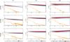 |
Fig. 21 Angular power spectra of odd−even year maps. Coloured lines represent the four nulls obtained from data and simulations of the effects listed in Table 2. The coloured area represents the envelope from Monte Carlo simulations as described in the text. |
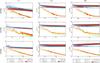 |
Fig. 22 Angular power spectra of consecutive survey difference maps. Coloured lines represent the four nulls obtained from data and simulations of the effects listed in Table 2. The coloured area represents the envelope from Monte Carlo simulations as described in the text. |
3.3.4. Highlighting straylight residuals with consecutive survey difference maps
We looked for residual effects in null maps constructed from differences between consecutive surveys, which we expect to be dominated by Galactic straylight. Indeed, when the spacecraft changes from an odd to an even survey, it re-visits the same sky patch with its orientation reversed by about 180°. As a consequence, the coupling of the beams with the sky is reversed, so that differences between odd and even surveys highlight the effect of main beam asymmetries and straylight from sidelobes. This implies that consecutive survey differences are among the most demanding null tests.
In Fig. 22 we display the angular power spectra of a wide sample of consecutive survey difference maps and compare them with noise and systematic effect simulations.
In this case, at 30GHz the null spectra from the data exceed the predictions from both the noise Monte Carlo and the systematic effects simulations that assume a perfect subtraction of straylight effects. This is true particularly for the spectra in temperature. Some excess in temperature is also present at 44 and 70GHz.
These results give useful hints on the accuracy of the optical model of the LFI sidelobes used to estimate the straylight contribution. In this respect we are planning further studies to improve this model by exploiting the information provided by these null tests. The outcome of these studies will be reported in the context of the next Planck release.
3.4. Impact of systematic effects on large angular scales
In this section we describe the assessment of systematic effect uncertainties on the detection of optical depth, τ, from LFI data on large angular scales. For the Planck 2015 release, the extraction of the τ parameter is based on the LFI 70GHz data, using the LFI 30GHz channel for removing polarized foreground synchrotron and the HFI 353GHz channel to clean polarized dust emission (Planck Collaboration XI 2016; Planck Collaboration XIII 2016).
To quantify the impact of residual effects on τ, we carried out an end-to-end analysis, propagating the simulated effects to maps, power spectra, and parameters, following the same processing steps as adopted in the data analysis. We start from the map containing the sum of all the systematic effects at 70GHz in polarization, add to it a realization of white noise and 1 /f noise derived from FFP8 simulations for the full mission, and finally add a CMB realization. The corresponding map at 30GHz is used in the template-fitting procedure to quantify its impact on the synchrotron removal process. Here we neglect the propagation of systematic effects from the 353GHz channel. However, we expect a very small contribution from this channel, considering the expected level of systematic effects (see Sect. 7 of Planck Collaboration VIII 2016) and the scaling coefficient for dust between 353 and 70GHz, β ≈ 0.0077 (Planck Collaboration XI 2016, Sect. 2.3).
In more detail, we consider the linear combination mclean = m70−αm30, where α = 0.063 is the effective synchrotron scaling ratio between the 30 and 70GHz channels, and adjust the effective noise covariance matrix accordingly (see Planck Collaboration XI 2016, for a more detailed discussion). In practice, this is equivalent to assuming that our cleaning procedure leaves no foreground residual in the final map, and for the scope of this analysis, we only need to consider the impact of the rescaled 30GHz noise and residual effects on the foreground-cleaned map.
From the resulting foreground-cleaned map, we extracted the power spectra for the temperature and polarization components at multipoles ℓ ≤ 29. We calculated the spectra over the sky region used to derive τ, shown in the bottom panel of Fig. 5.
To quantify the result, we calculated the bias introduced by the systematic effects on the three parameters that are most sensitive to low multipoles, i.e., τ, r, and the amplitude of scalar perturbations, As. We produced 1000 Monte Carlo FFP8 simulations of the CMB polarized sky plus white and 1 /f noise with systematic effects and 1000 similar simulations but containing only CMB and noise. For each realization we then calculated the marginalized distributions for each of the three parameters X = τ,r,As and calculate the differences ΔX = Xsyst.−Xno−syst., which represent the bias introduced in the estimates of X by the combination of all systematic effects.
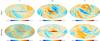 |
Fig. 23 Maps in total intensity and polarization of the LFI systematic effects after component separation. Top: maps extracted with NILC. Bottom: maps extracted with SEVEM. The colour scale of SEVEM maps is five times smaller than that of NILC maps. |
For log (As) and r we find median bias values of −0.026 and 0.11, respectively, which would correspond to a 0.2σ effect on the amplitude parameter and an increase of 15% on the upper limit on r (95% CL). However, the dominant Planck constraints on these two parameters actually come from temperature power spectrum at high multipoles, so the actual impact on the Planck results is very small.
For the optical depth, we find a mean bias ⟨ Δτ ⟩ = 0.005, or 0.2–0.25 times the standard deviation of the value of τ measured by LFI (Planck Collaboration XIII 2016). This result shows that the impact of all systematic effects on the measurement of τ is within 1σ. The measured ⟨ Δτ ⟩ is compatible with a positive but sub-dominant bias by residual systematics, with an impact on τ that is within the statistical uncertainty.
We emphasize that this result is based on our bottom-up approach, and therefore it relies on the accuracy and completeness of our model of all known instrumental systematic effects. As we have shown, on large angular scales, systematics residuals from our model are only marginally dominated by the EE polarized CMB signal. For this reason we plan to produce further independent tests on these data based both on null tests and on cross-spectra between the 70GHz map and the HFI 100 and 143GHz maps. Such a cross-instrument approach may prove particularly effective, because we expect that systematic effects between the two Planck instruments are largely uncorrelated. We will discuss these analyses in a forthcoming paper in combination with the release of the low-ell HFI polarization data at 100–217GHz and in the final 2016 Planck release.
3.5. Propagation of systematic effects through component separation
In this section we discuss how we assess the impact of residual systematic effects in the LFI data on the CMB power spectra after component separation (see Fig. 27 in Sect. 4).
Planck component separation exploits a set of algorithms to derive each individual sky emission component. They are minimum variance in the needlet domain (NILC), or they use foreground templates generally based on differences between two Planck maps that are close in frequency (SEVEM), as well as parametric fitting conducted in the pixel (Commander) and harmonic (SMICA) domains. We describe them in detail in Planck Collaboration IX (2016).
To assess residuals after component separation, we use LFI systematic effect maps as the input for a given algorithm, setting the HFI channels to zero. This means that the output represents only the LFI systematic uncertainty in the corresponding CMB reconstruction. In Planck Collaboration III (2014), we exploited a global minimum-variance component-separation implementation, AltICA, to derive weights used to combine the LFI systematic effect maps. Here we generalize the same procedure using NILC and SEVEM. Both are based on minimum-variance estimation of the weights, but in localized spatial and harmonic domains, and so optimally subtract foregrounds where they are most relevant (NILC), and exploit foreground templates generally constructed by diffferencing two nearby Planck frequency channels (SEVEM).
Figure 23 shows maps in total intensity and polarization of the LFI systematic effects after component separation. Maps extracted with NILC appear in the top row, while maps extracted with SEVEM appear in the bottom row. The structures that are most prominent outside the Galactic residuals appear to be associated with the scan strategy. Residuals are about five times larger for NILC than for SEVEM for the reasons described in Sect. 4. It is important to stress that component separation does not alter the relative strength of the various systmatic effects treated in this paper, but simply filters them through the given foreground-cleaning pipeline.
Figure 27 in Sect. 4 shows power spectra obtained from these maps compared with the best-fit Planck 2015 ΛCDM cosmology. To calculate these spectra we first applied the masks shown in Fig. 5 and then computed pseudo-spectra corrected for the unseen sky fraction.
In total intensity we confirm the results presented in Planck Collaboration III (2014): the impact of known LFI systematic effects is at least two orders of magnitude less than the CMB. In polarization we observe a different residual level, depending on the algorithm used. The weighting strategy of NILC on large angular scales performed in the needlet domain yields a residual effect that is larger by about 1.5 orders of magnitude compared to SEVEM. We further discuss this discrepancy in Sect. 4. The 70-GHz channel is one with less foreground contamination and higher angular resolution. As a result, NILC weights this channel more than do the others. This ultimately causes a higher level of residual systematic effects.
The residual effect in polarization after processing with NILC is comparable to interesting levels of cosmological B-modes on large scales. This particular point needs further attention for the next Planck data release, where component-separation solutions will be relevant for characterizing polarization accurately on large angular scales.
3.6. Gaussianity statistical tests
In this section we present the results of statistical tests assessing the impact of known systematic effects in the LFI data on non-Gaussianity studies.
The presence of systematic effect residuals can bias the statistical isotropy properties of the Planck maps (Planck Collaboration XVI 2016) or the constraints on primordial non-Gaussianity (Planck Collaboration XVII 2016). Therefore it is important to understand the impact of known systematic effects on the most relevant non-Gaussianity studies carried out within this release.
In the Planck 2013 release, the non-Gaussianity studies were carried out using temperature data in two steps (Planck Collaboration III 2014). First, we estimated an upper limit on the “detectability level” of all the known effects summed into a single “global” map. This level was defined as the factor we must multiply the global map by to generate a significant non-Gaussian deviation. Second, we measured the bias that these systematic effects could introduce on the local nonlinear coupling fNL parameter.
In the current release we follow the same approach, additionally considering the polarization signal at low ℓ. We have also considered the three usual cases (namely local, equilateral, and orthogonal) for the bispectrum shape when defining fNL.
We characterize the level of detectability of the non-Gaussian contamination by comparing simulations that contain the systematic effect map added and rescaled by a global factor, fsys, with the null hypothesis (i.e., no systematic effects). We consider two scenarios, measuring the level of detectability of the systematic effects over (i) the CMB + noise background; and (ii) the noise background alone. These can be written as 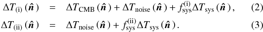 For each case we calculated the detectability factor using a χ2 test on Monte Carlo simulations. First we produced two sets of 1000 simulations with and without the systematic effects added, and then we defined χ2 = VC-1VT. The vector V can be V = [T], V = [Q,U], or V = [T,Q,U], while C is the corresponding covariance matrix. Under the assumption of normality, these statistics follow a χ2 distribution with NT, NQ + NU or NT + NQ + NU degrees of freedom, respectively14. This is one of the estimators used in the Gaussianity analyses of Planck Collaboration XVI (2016).
To define the “detectability factors”  and
and  we consider a method of discriminating two χ2 histograms corresponding to simulations with and without systematic contamination. We use the common choice based on the significance level of the two histograms, defined as the fraction of cases of the null hypothesis (no systematic effects added) with a χ2 greater than the median of the alternative hypothesis (systematic effects added). Both distributions are considered different when this number is lower than 5%. Therefore and are defined as the global scaling factor of the systematic map that is needed to detect non-Gaussianity deviations with 95% confidence.
Level of detectability of non-Gaussianity caused by simulated systematic effects in the LFI maps.
We measured the levels of detectability, reported in Table 3, for temperature and polarization maps at low resolution (ℓmax = 95). For temperature-only we obtained  16.34, 9.06, and 12.98 for 30, 44, and 70GHz, respectively. These values are consistent with those obtained in the previous release (Planck Collaboration III 2014). Including polarization results in lower levels being detectable for both cases (CMB plus noise and noise-only backgrounds). The values found are
  0.73, 1.25, and 1.81 for 30, 44, and 70GHz, respectively. If we only consider the noise background the values decrease for all the cases (see Table 3). The level of detectability for the 70GHz channel in the CMB plus noise background case is always greater than the critical limit of
  . This is the case that is particularly relevant for non-Gaussianity tests (Planck Collaboration XVI 2016; Planck Collaboration XVII 2016).
The second aspect of non-Gaussianity we have considered is the impact of systematic effects on the primordial non-Gaussianity fNL parameter. We define the bias on this parameter, ΔfNL, as the mean difference between the two fNL values measured in maps with and without systematic effects, i.e., 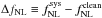 .
.
To obtain a limit on this bias, we first computed the full-sky bispectrum of the global systematic effect maps, following the formalism of Komatsu et al. (2002), and then we cross-correlated it with the primordial bispectrum. We removed the bias generated by extragalactic point sources or the CIB-lensing, following the procedure described, e.g., in Curto et al. (2013, 2015).
Table 4 shows the values of the bias ΔfNL calculated at high resolution (ℓmax = 1024) for the LFI channels. The bias is normalized to the corresponding dispersion of fNL to estimate the relative impact on the measurement of this parameter. For the three LFI channels, the impact of systematic effects on fNL is negligible, since lower than 0.90% for the local shape, 1.80% for the equilateral shape and 2.22% for the orthogonal shape. The 30GHz channel has the highest amplitude for this bias, whereas the 44 and 70GHz channels have maximum amplitudes of 0.02% and 0.03%, respectively.
4. Summary of uncertainties due to systematic effects
This section provides a top-level overview of the residual15 uncertainties in the Planck-LFI CMB maps and power spectra, introduced by systematic effects. We list these effects in Table 1 and summarize the main results of our analysis, which are discussed in Sect. 3 and the corresponding sections.
Relative variation ΔfNL/σ(fNL) as a percentage, caused by simulated systematic effects in the LFI data.
Tables 5−7 report the peak-to-peak16 and rms systematic effect uncertainties in LFI maps. To calculate these uncertainties we used HEALPix (Górski et al. 2005) maps with simulated systematic effects degraded to Nside = 128 (corresponding to a pixel size of around 28′) at 30 and 44GHz, and Nside = 256 (corresponding to a pixel size of about 14′) at 70GHz. These pixel sizes approximate the optical beam angular resolution. Maps were masked with the top and middle masks shown in Fig. 5, also used for power spectra estimation.
Summary of systematic effect uncertainties on 30GHz maps inμKCMB.
Summary of systematic effect uncertainties on 44GHz maps inμKCMB.
Summary of systematic effect uncertainties on 70GHz maps inμKCMB.
The rms uncertainty in LFI maps from known systematic effects is ≲0.5μK in polarization and ≲1μK in temperature. The improvements17 introduced into the LFI pipeline have allowed us to reduce the peak-to-peak uncertainty by a factor ranging from 3.5 at 70GHz to 7.7 at 30GHz, compared to the 2013 analysis (Planck Collaboration III 2014). At 30 and 70GHz, calibration and analogue-to-digital converter (ADC) nonlinearity are the prevailing effects, while calibration and 1-Hz spikes dominate at 44GHz.
In our assessment we have not included the residual effects from far sidelobes, because we remove Galactic straylight directly from the timelines. This removal is based on optical simulations, which implies that a residual effect may be present in the data. Estimating this remaining signal is complex and computationally demanding, since it requires us to generate Monte Carlo simulations of the far sidelobes. For the present analysis we have used the following approach regarding far sidelobes: we assessed the impact of systematic effects assuming the perfect removal of Galactic straylight; and additionally we quantified how much the far sidelobes would affect our results if they were not removed at all.
Figures 24−26 provide an overview of the power spectra in temperature and polarization for each systematic effect, compared to the foreground levels at 30GHz and to the cosmological signal at 44 and 70GHz. At 30GHz we use the spectrum obtained from measured data as an approximation of the foreground spectrum at this frequency. At 44 and 70GHz we use the power spectrum coming from the best fits to the Planck cosmological parameters (see Figs. 9 and 10 in Planck Collaboration I 2016) filtered by the LFI window functions. The example CMB B-mode spectrum is based on Planck-derived cosmological parameters, and it assumes a tensor-to-scalar ratio r = 0.1, a tensor spectral index nT = 0, and no beam-filtering. Instrumental noise here is based on “half-ring” difference maps, as described in Sects. 12.1 and 12.2 of Planck Collaboration II (2016).
In the same figure we also show the power spectra of Galactic straylight detected by the far sidelobes (the dotted green lines), which indicate the level of the effect that we expect to have removed from the data.
At 30GHz the systematic effects are all lower than the foreground signal. The Galactic straylight is higher than the noise level at ℓ ≲ 20. For this reason we removed an estimate of Galactic straylight from the timelines, based on our best knowledge of the far sidelobes. These results show that the 30GHz channel gives a reliable foreground template, with uncertainties set by the instrumental noise.
At 44 and 70GHz the level of Galactic straylight is lower than the CMB. It is reasonable to assume that any residual that could be present in the data must be less than the total effect reported here and, therefore, negligible compared to the CMB.
The power spectrum of the sum of all systematic effects (dark-grey line) is higher than the E-mode spectrum in the ℓ range 10–15 and is marginally below that for multipoles <10, at both 44 and 70GHz. This could have an impact on the extraction of the optical depth, τ, which is strongly dependent on the  spectrum at very low ℓs.
We have evaluated the impact of the simulated effects on τ (see Sect. 3.4) and found a bias that is about 0.2 times the standard deviation, showing that the uncertainty on this parameter is dominated by statistics and the contribution from systematic effects is only of marginal importance.
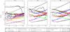 |
Fig. 24 Angular power spectra of the various systematic effects at 30GHz, compared to the CMB and foreground temperature and polarization spectra and to the instrumental noise from half-ring (HR) difference maps. The CMB TT and EE spectra are best fits to the Planck cosmological parameters (see Figs. 9 and 10 in Planck Collaboration I 2016) filtered by the LFI window functions. The example CMB B-mode spectrum is based on Planck-derived cosmological parameters and assumes a tensor-to-scalar ratio r = 0.1, a tensor spectral index nT = 0, and no beam-filtering. The thick dark-grey line represents the total contribution. The dotted dark-green line is the contribution from the far sidelobes that has been removed from the data and is therefore not considered in the total. |
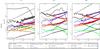 |
Fig. 25 Angular power spectra of the various systematic effects at 44GHz, compared to the CMB temperature and polarization spectra and to the instrumental noise from half-ring (HR) difference maps. The CMB TT and EE spectra are best fits to the Planck cosmological parameters (see Figs. 9 and 10 in Planck Collaboration I 2016) filtered by the LFI window functions. The example CMB B-mode spectrum is based on Planck-derived cosmological parameters and assumes a tensor-to-scalar ratio r = 0.1, a tensor spectral index nT = 0, and no beam-filtering. The thick dark-grey line represents the total contribution. The dotted dark-green line is the contribution from far the sidelobes that has been removed from the data and is therefore not considered in the total. |
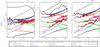 |
Fig. 26 Angular power spectra of the various systematic effects at 70GHz, compared to the CMB temperature and polarization spectra and to the instrumental noise from half-ring (HR) difference maps. The CMB TT and EE spectra are best fits to the Planck cosmological parameters (see Figs. 9 and 10 in Planck Collaboration I 2016) filtered by the LFI window functions. The example CMB B-mode spectrum is based on Planck-derived cosmological parameters and assumes a tensor-to-scalar ratio r = 0.1, a tensor spectral index nT = 0, and no beam-filtering. The thick dark-grey line represents the total contribution. The dotted dark-green line is the contribution from far the sidelobes that has been removed from the data and is therefore not considered in the total. |
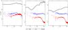 |
Fig. 27 Angular power spectra for the combined LFI systematic effects templates in the CMB TT, EE, and BB reconstructions of the NILC and SEVEM pipelines, compared with the Planck fiducial cosmology. |
We also assessed the uncertainty caused by LFI systematic effects on the CMB power spectra estimated by Planck after component separation.
In our procedure (described in Sect. 3.5), we set the HFI channels to zero to evaluate the systematic uncertainty of LFI only in the CMB reconstruction. It is a generalization of the approach described in Planck Collaboration III (2014), based on component-separation weights calculated via minimum variance over the whole sky area being considered. In this test we first input maps with the sum of all systematic effects into the component separation pipeline, then we applied the top and middle masks in Fig. 5 to the resulting maps, and finally, we calculated the pseudo-spectra.
Figure 27 shows the angular power spectra of the sum of all known LFI systematic effects in the component-separation outputs of the NILC and SEVEM algorithms described in Planck Collaboration IX (2016). These plots highlight the level of the residual effects compared with the Planck 2015 best-fit cosmology.
The results in total intensity confirm the findings of our previous data release. The residual systematic effects are several orders of magnitude lower than the CMB power spectrum on all angular scales.
The results in polarization show that the residual effects resulting after the application of the SEVEM algorithm are about 1.5–2 orders of magnitude lower than those resulting from NILC on all angular scales. This means that the residual effects obtained with NILC have an amplitude that is comparable to cosmological B-modes with r ~ 0.1.
The reason for this discrepancy in the component-separated outputs is the different weighting that the two codes apply to the LFI channels. In NILC the LFI channels are weighted more than in SEVEM, which also implies a larger impact of the systematic effects. We now recall the reasons for this different weighting.
NILC implements a minimum variance approach in the needlet domain, and produces a set of weights for each ℓ band in which it is applied. For this reason, in the LFI channels the weights are particularly relevant on large angular scales, where foregrounds are most important.
SEVEM, on the other hand, applies a smoothing to the LFI channels and then calculates the minimum variance coefficients over the entire range of multipoles, which eventually results in smaller weights for the LFI channels and, therefore, a smaller contribution of their systematic effects.
5. Conclusions
This is the era of precision cosmology. The advances in detector and space technology in the past 20 years now allow us to test theories that describe the evolution of the Universe with statistical uncertainties that were unimaginable at the time the CMB was discovered, more than 50 years ago.
Planck has produced the most sensitive full-sky maps of the microwave sky to date. We have exploited its unprecedented statistical power to obtain the most precise angular temperature power spectrum of the CMB (Planck Collaboration XI 2016), as well as cosmological parameters with relative errors below the percent level in some cases (Planck Collaboration XIII 2016).
In the past ten years several experiments from the ground and the stratosphere have successfully tested new technologies that are further increasing sensitivity and opening new frontiers for cosmology by exploiting measurements of the CMB anisotropy polarization.
However, precision is nothing without accuracy. Understanding and controlling systematic uncertainties is one of the greatest challenges for present and future measurements of the CMB. The control of systematic effects has indeed been a challenge for Planck, both in the development phase and during data analysis.
In this paper we have discussed the systematic effect uncertainties of the Planck Low Frequency Instrument data in the context of the second cosmological data release. This is the result of work begun almost 20 yr ago, when we started developing the instrument with systematic effects control as one of the main drivers for the instrument and data-analysis pipeline designs.
Our approach followed two complementary paths.
-
The first uses measured data and exploits the redundancy in thescanning strategy to divide the observations into periods ofvarious lengths in which the observed sky is the same. We used theanalysis of difference maps constructed on such periods (“nulltests”) to highlight possible spurious residual signals exceedingthe instrumental noise.
-
The second used our knowledge of the instrument to build physical models of the various known systematic effects that are simulated from timelines to maps. Here we exploit, as much as possible, actual flight measurements, such as pointing, temperatures, and radiometric data.
We used simulations to quantify the uncertainties introduced by systematic effects in the maps and power spectra, and compared our predictions with null-test results to identify residuals that are not accounted for by our model. We also used our simulations to assess the impact of these effects on cosmological parameters (like the reionization optical depth, τ) on the measurements of the CMB statistical properties and on component separation.
Our results for temperature data confirm the findings of the first Planck release (Planck Collaboration III 2014): the measurements are limited by instrumental noise, and on all relevant angular scales, the systematic effects are several orders of magnitude below the power spectrum of the CMB itself.
Our analysis for polarization demonstrates the robustness of the LFI data for scientific analysis, in particular regarding the measurement of τ and the statistical analysis of CMB maps. Systematic effects, however, are more challenging in polarization than in temperature and their level is close to the E-mode signal, especially on large angular scales.
Uncertainties in the relative photometric calibrations dominate the LFI systematic effects budget, especially on large angular scales. This is an area in the data analysis pipeline that is still being improved in preparation for the next Planck release.
Our data could also contain residual Galactic straylight caused by an imperfect knowledge of the beam sidelobes. We do not consider this residual in our budget, but null spectra from consecutive surveys indicate the possible presence of such a spurious signal at 30GHz.
At 70GHz the systematic effects compete with the CMB E-modes for multipoles in the range 10–20. This does not preclude an accurate measurement of τ, which depends mainly on multipoles ℓ< 10 (Planck Collaboration XI 2016). Using systematic effects simulations we showed that the bias introduced on τ is less than 0.25 times the standard deviation of the measured parameter. Forthcoming analyses will include independent estimates, based on null tests and on cross-correlation between the LFI 70GHz map and the HFI 100 and 143GHz maps.
We also evaluated the impact on the scalar perturbations amplitude, ln(As), and on the upper limit to the tensor-to-scalar ratio, r, derived with large-scale polarization data. In this case the effect on ln(As) is approximately 0.2σ, while the upper limit on r is increased by the systematic effects by around 15%. For these two parameters, however, the main Planck constraint comes from the temperature power spectrum at high multipoles, so that the actual impact is negligible.
At 30GHz the systematic effects are much smaller than the Galactic emission at all multipoles. We use this channel as a foreground monitor, which implies that we are not limited by systematic effects at this frequency for any angular scale, in either temperature or polarization.
The 44GHz channel displays residuals that compete with the E-mode polarization for ℓ ≤ 10 and dominate the signal for multipoles in the range 10–20. We did not use this channel in the current polarization analysis, so these effects do not play a role in the measurement of τ. We uses the 44GHz data, however, in the component separation analysis.
The contribution of LFI systematic effects on CMB maps and power spectra after component separation is smaller than the CMB signal on all scales, both in temperature and polarization. We assessed this using two component separation codes, namely NILC (a minimum variance code in the needlet domain) and SEVEM (a code based on foreground templates). With both codes the LFI systematic uncertainties do not limit accurate measurement of the CMB temperature and polarization spectra. As expected, we find that the use of SEVEM results in a lower level of residuals compared to NILC, because of the different weighting of the LFI data applied by the two codes.
The presence of known systematic effects in the LFI data does not significantly affect non-Gaussianity studies. We have used maps with the simulated effects combined with CMB and noise maps and found that, at 70GHz, the amplitude of these effects must be at least a factor of 2 larger to detect a significant non-Gaussianity. We have also assessed the bias on the fNL parameter and found that it is less than 0.1% at 44 and 70GHz and <2.2% at 30GHz.
Finally, we comment about the systematic uncertainties on the B-mode polarization measurements. Our analysis shows that at 70GHz the level of systematic effects is lower than the instrumental noise, but higher than a B-mode power spectrum for r = 0.1. This does not affect our polarization analysis, based on E-mode polarization data, but once again shows the importance of understanding and controlling systematic effects in future experiments aiming at the detection of this elusive signal.
Understanding and controlling systematic effects in the LFI data has been a challenge from which we have gained even deeper knowledge of our instrument and learned several valuable lessons for the future. This is destined to be a future of even more precise and accurate cosmology, and also one of increasing challenge to control systematics effects.
Planck (http://www.esa.int/Planck) is a project of the European Space Agency (ESA) with instruments provided by two scientific consortia funded by ESA member states and led by Principal Investigators from France and Italy, telescope reflectors provided through a collaboration between ESA and a scientific consortium led and funded by Denmark, and additional contributions from NASA (USA).
A null map is the difference between maps over time periods in which the sky signal is the same. See Sect. 3.3.
For the definition of the main- and sub-reflector spillovers refer to Fig. 7 of Planck Collaboration III (2014).
The main beam is defined as extending to 1.9, 1.3, and 0.9° at 30, 44, and 70GHz, respectively.
Here we refer to both the beams simulated with GRASP and to those reconstructed from Jupiter transits.
The polarization angle is defined as ψpol = arctan(Erhc/Elhc). Here Erhc and Elhc are the right- and left-hand circularly polarized components of the field, which can be defined in terms of the co- and cross-polar components, Eco and Ecx, as Erhc(lhc) = (Eco−(+)Ecx)/ (TICRA Engineering Consultants 2008).
We have implemented these improvements into a new module named DaCapo, described in Sect. 7.1 of Planck Collaboration II (2016).
Because difference maps may contain unobserved pixels, in each null test we take the union between this mask and any set of unobserved pixels. For example, maps of single surveys do not cover the full sky, which requires us to combine the mask with the unobserved pixels in the null map.
In this step we use the conviqt_v4 and multimod routines (Reinecke et al. 2006) with parameters reported in Table 6 of Planck Collaboration IV (2016).
Multi-reflector geometrical theory of diffraction (TICRA Engineering Consultants 2012).
We do not expect that single radiometer survey differences are strictly null. Indeed, the radiometers are polarized detectors that observe the sky with different ranges of polarization angles for different surveys. We use these tests to validate the radiometer stability, minimizing these effects by considering survey combinations with the same scanning patterns (survey 1 vs. survey 3, survey 2 vs. survey 4) or by combining radiometers to solve for I, Q and U.
NT, NQ, and NU are the total number of pixels available for the T, Q, and U maps, respectively.
We use the word “residual” to refer to the spurious signal remaining in the final LFI maps due to a systematic effect, which is after any removal steps applied by the data analysis pipeline.
In this paper we call “peak-to-peak” the difference between the 99% and the 1% quantiles of the pixel value distributions.
See Sects. 4, 6, and 7 of Planck Collaboration II (2016).
Acknowledgments
The Planck Collaboration acknowledges the support of: ESA; CNES, and CNRS/INSU-IN2P3-INP (France); ASI, CNR, and INAF (Italy); NASA and DoE (USA); STFC and UKSA (UK); CSIC, MINECO, JA, and RES (Spain); Tekes, AoF, and CSC (Finland); DLR and MPG (Germany); CSA (Canada); DTU Space (Denmark); SER/SSO (Switzerland); RCN (Norway); SFI (Ireland); FCT/MCTES (Portugal); ERC and PRACE (EU). A description of the Planck Collaboration and a list of its members, indicating which technical or scientific activities they have been involved in, can be found at http://www.cosmos.esa.int/web/planck/planck_collaboration. Some of the results in this paper have been derived using the HEALPix package.
References
- Aumont, J., Conversi, L., Thum, C., et al. 2010, A&A, 514, A70 [NASA ADS] [CrossRef] [EDP Sciences] [Google Scholar]
- Bersanelli, M., Mandolesi, N., Butler, R. C., et al. 2010, A&A, 520, A4 [NASA ADS] [CrossRef] [EDP Sciences] [Google Scholar]
- Burigana, C., Sandri, M., Villa, F., et al. 2004, A&A, 428, 311 [NASA ADS] [CrossRef] [EDP Sciences] [Google Scholar]
- Curto, A., Tucci, M., González-Nuevo, J., et al. 2013, MNRAS, 432, 728 [NASA ADS] [CrossRef] [Google Scholar]
- Curto, A., Tucci, M., Kunz, M., & Martinez-Gonzalez, E. 2015, MNRAS, 450, 3778 [NASA ADS] [CrossRef] [Google Scholar]
- Górski, K. M., Hivon, E., Banday, A. J., et al. 2005, ApJ, 622, 759 [NASA ADS] [CrossRef] [Google Scholar]
- Gregorio, A., Cuttaia, F., Mennella, A., et al. 2013, J. Instr., 8, 7001 [NASA ADS] [CrossRef] [Google Scholar]
- Hinshaw, G., Weiland, J. L., Hill, R. S., et al. 2009, ApJS, 180, 225 [NASA ADS] [CrossRef] [Google Scholar]
- Keihänen, E., Keskitalo, R., Kurki-Suonio, H., Poutanen, T., & Sirviö, A. 2010, A&A, 510, A57 [NASA ADS] [CrossRef] [EDP Sciences] [Google Scholar]
- Komatsu, E., Wandelt, B. D., Spergel, D. N., Banday, A. J., & Górski, K. M. 2002, ApJ, 566, 19 [NASA ADS] [CrossRef] [Google Scholar]
- Kurki-Suonio, H., Keihänen, E., Keskitalo, R., et al. 2009, A&A, 506, 1511 [NASA ADS] [CrossRef] [EDP Sciences] [Google Scholar]
- Lamarre, J., Puget, J., Ade, P. A. R., et al. 2010, A&A, 520, A9 [NASA ADS] [CrossRef] [EDP Sciences] [Google Scholar]
- Leahy, J. P., Bersanelli, M., D’Arcangelo, O., et al. 2010, A&A, 520, A8 [NASA ADS] [CrossRef] [EDP Sciences] [Google Scholar]
- Mennella, A., Bersanelli, M., Butler, R. C., et al. 2010, A&A, 520, A5 [NASA ADS] [CrossRef] [EDP Sciences] [Google Scholar]
- Mennella, A., Butler, R. C., Curto, A., et al. 2011, A&A, 536, A3 [NASA ADS] [CrossRef] [EDP Sciences] [Google Scholar]
- Planck Collaboration ES. 2015, The Explanatory Supplement to the Planck 2015 results, http://wiki.cosmos.esa.int/planckpla/index.php/Main_Page (ESA) [Google Scholar]
- Planck Collaboration II. 2011, A&A, 536, A2 [NASA ADS] [CrossRef] [EDP Sciences] [Google Scholar]
- Planck Collaboration I. 2014, A&A, 571, A1 [NASA ADS] [CrossRef] [EDP Sciences] [Google Scholar]
- Planck Collaboration III. 2014, A&A, 571, A3 [NASA ADS] [CrossRef] [EDP Sciences] [Google Scholar]
- Planck Collaboration V. 2014, A&A, 571, A5 [NASA ADS] [CrossRef] [EDP Sciences] [Google Scholar]
- Planck Collaboration XII. 2014, A&A, 571, A12 [NASA ADS] [CrossRef] [EDP Sciences] [Google Scholar]
- Planck Collaboration I. 2016, A&A, 594, A1 [NASA ADS] [CrossRef] [EDP Sciences] [Google Scholar]
- Planck Collaboration II. 2016, A&A, 594, A2 [NASA ADS] [CrossRef] [EDP Sciences] [Google Scholar]
- Planck Collaboration III. 2016, A&A, 594, A3 [NASA ADS] [CrossRef] [EDP Sciences] [Google Scholar]
- Planck Collaboration IV. 2016, A&A, 594, A4 [NASA ADS] [CrossRef] [EDP Sciences] [Google Scholar]
- Planck Collaboration V. 2016, A&A, 594, A5 [NASA ADS] [CrossRef] [EDP Sciences] [Google Scholar]
- Planck Collaboration VI. 2016, A&A, 594, A6 [NASA ADS] [CrossRef] [EDP Sciences] [Google Scholar]
- Planck Collaboration VII. 2016, A&A, 594, A7 [NASA ADS] [CrossRef] [EDP Sciences] [Google Scholar]
- Planck Collaboration VIII. 2016, A&A, 594, A8 [NASA ADS] [CrossRef] [EDP Sciences] [Google Scholar]
- Planck Collaboration IX. 2016, A&A, 594, A9 [NASA ADS] [CrossRef] [EDP Sciences] [Google Scholar]
- Planck Collaboration X. 2016, A&A, 594, A10 [NASA ADS] [CrossRef] [EDP Sciences] [Google Scholar]
- Planck Collaboration XI. 2016, A&A, 594, A11 [NASA ADS] [CrossRef] [EDP Sciences] [Google Scholar]
- Planck Collaboration XII. 2016, A&A, 594, A12 [NASA ADS] [CrossRef] [EDP Sciences] [Google Scholar]
- Planck Collaboration XIII. 2016, A&A, 594, A13 [NASA ADS] [CrossRef] [EDP Sciences] [Google Scholar]
- Planck Collaboration XIV. 2016, A&A, 594, A14 [NASA ADS] [CrossRef] [EDP Sciences] [Google Scholar]
- Planck Collaboration XV. 2016, A&A, 594, A15 [NASA ADS] [CrossRef] [EDP Sciences] [Google Scholar]
- Planck Collaboration XVI. 2016, A&A, 594, A16 [NASA ADS] [CrossRef] [EDP Sciences] [Google Scholar]
- Planck Collaboration XVII. 2016, A&A, 594, A17 [NASA ADS] [CrossRef] [EDP Sciences] [Google Scholar]
- Planck Collaboration XVIII. 2016, A&A, 594, A18 [NASA ADS] [CrossRef] [EDP Sciences] [Google Scholar]
- Planck Collaboration XIX. 2016, A&A, 594, A19 [NASA ADS] [CrossRef] [EDP Sciences] [Google Scholar]
- Planck Collaboration XX. 2016, A&A, 594, A20 [NASA ADS] [CrossRef] [EDP Sciences] [Google Scholar]
- Planck Collaboration XXI. 2016, A&A, 594, A21 [NASA ADS] [CrossRef] [EDP Sciences] [Google Scholar]
- Planck Collaboration XXII. 2016, A&A, 594, A22 [NASA ADS] [CrossRef] [EDP Sciences] [Google Scholar]
- Planck Collaboration XXIII. 2016, A&A, 594, A23 [NASA ADS] [CrossRef] [EDP Sciences] [Google Scholar]
- Planck Collaboration XXIV. 2016, A&A, 594, A24 [NASA ADS] [CrossRef] [EDP Sciences] [Google Scholar]
- Planck Collaboration XXV. 2016, A&A, 594, A25 [NASA ADS] [CrossRef] [EDP Sciences] [Google Scholar]
- Planck Collaboration XXVI. 2016, A&A, 594, A26 [NASA ADS] [CrossRef] [EDP Sciences] [Google Scholar]
- Planck Collaboration XXVII. 2016, A&A, 594, A27 [NASA ADS] [CrossRef] [EDP Sciences] [Google Scholar]
- Planck Collaboration XXVIII. 2016, A&A, 594, A28 [NASA ADS] [CrossRef] [EDP Sciences] [Google Scholar]
- Reinecke, M., Dolag, K., Hell, R., Bartelmann, M., & Enßlin, T. A. 2006, A&A, 445, 373 [NASA ADS] [CrossRef] [EDP Sciences] [Google Scholar]
- Sandri, M., Villa, F., Nesti, R., et al. 2004, A&A, 428, 299 [NASA ADS] [CrossRef] [EDP Sciences] [Google Scholar]
- Sandri, M., Villa, F., Bersanelli, M., et al. 2010, A&A, 520, A7 [NASA ADS] [CrossRef] [EDP Sciences] [Google Scholar]
- Seiffert, M., Mennella, A., Burigana, C., et al. 2002, A&A, 391, 1185 [NASA ADS] [CrossRef] [EDP Sciences] [Google Scholar]
- Terenzi, L., Salmon, M. J., Colin, A., et al. 2009, J. Instr., 4, 2012 [NASA ADS] [Google Scholar]
- TICRA Engineering Consultants 2008, GRASP, technical descritpion (Knud Pontoppidan, TICRA, Denmark) [Google Scholar]
- TICRA Engineering Consultants 2012, GRASP Multi-GTD add-on (Knud Pontoppidan, TICRA, Denmark) [Google Scholar]
- Tomasi, M., Cappellini, B., Gregorio, A., et al. 2010, J. Instr., 5, 1002 [Google Scholar]
- Villa, F., Pagan, L., & Sandri, M. 2005, LFI alignment evaluation and recovery proposal, Tech. Rep. PL-LFI-PST-TN-054, LFI [Google Scholar]
- Zacchei, A., Maino, D., Baccigalupi, C., et al. 2011, A&A, 536, A5 [NASA ADS] [CrossRef] [EDP Sciences] [Google Scholar]
All Tables
Level of detectability of non-Gaussianity caused by simulated systematic effects in the LFI maps.
Relative variation ΔfNL/σ(fNL) as a percentage, caused by simulated systematic effects in the LFI data.
All Figures
|
Fig. 1 Example of a cut of the simulated beam pattern of the 70GHz LFI18-S radiometer. The cut passes through the main reflector spillover of the Planck telescope. The plot shows, in particular, the level and shape of the near sidelobes. |
| In the text | |
|
Fig. 2 Definition of polarization angle. Left: the orientation of the main beam frame, (XYZ)MB, with respect to the line-of-sight (LOS) frame, (XYZ)LOS, is defined by the three angles θuv, φuv, and ψuv. The intermediate frame, (XYZ)DX, is the detector frame, defined by the two angles θuv and φuv. Right: the angle ψpol is defined with respect to XMB and represents the orientation of the polarization ellipse along the beam line of sight. It is very close to 0 or 90 deg for the S and M radiometers, respectively. |
| In the text | |
|
Fig. 3 Crab Nebula polarization angle measured by the various feedhorns in the focal plane. The straight horizontal line reports the value from Aumont et al. (2010) converted to Galactic coordinates, and the yellow area is the ± 1σ uncertainty. |
| In the text | |
|
Fig. 4 Simulated polarization angles and error bars from the Crab measurements used in the analysis. Top: radiometer main arm. Bottom: radiometer side arm. The scatter of the plotted angles is much less than the error bars because the uncertainty in our simulations is much smaller than the error bars derived from Crab measurements. |
| In the text | |
|
Fig. 5 Masks used in this work. Top: mask used to compute power spectra of simulated systematic effect total intensity maps. Middle: mask used to compute power spectra of Q and U systematic-effect maps. Bottom: mask used to compute power spectra of null maps. |
| In the text | |
|
Fig. 6 Uncertainty in the power spectra of the effect from far sidelobes introduced by the first-order approximation in GRASP simulations. Top: TT spectrum. Middle: EE spectrum. Bottom: BB spectrum. For each frequency the coloured area is the region between the native power spectrum and the one rescaled to account for the missing power. |
| In the text | |
|
Fig. 7 Maps of the effect from far sidelobes. Rows correspond to 30, 44, and 70GHz channels, while columns correspond to I, Q, and U. The straylight signal at 30GHz is larger compared to 44 and 70GHz. The 44GHz channel is the least contaminated by this effect. This behaviour results from the combination of the beam far sidelobes and the intensity of the Galactic emissions at the LFI frequencies. |
| In the text | |
|
Fig. 8 Maps of the effect from near sidelobes. Rows correspond to 30, 44, and 70GHz channels, while columns correspond to I, Q, and U. |
| In the text | |
|
Fig. 9 Maps of the effect from uncertainty in the polarization angle. The maps shown are randomly selected from one of the five tested realizations. Rows correspond to 30, 44, and 70GHz channels, while columns correspond to I, Q, and U. |
| In the text | |
|
Fig. 10 Peak-to-peak value of the effect from polarization angle uncertainty on LFI maps. The error bars represent the dispersion of the five cases chosen in the analysis. Top: total intensity. Bottom: Q and U Stokes parameters. |
| In the text | |
|
Fig. 11 Rms of the effect from polarization angle uncertainty on LFI maps. The error bars represent the dispersion of the five cases chosen in the analysis. Top: total intensity. Bottom: Q and U Stokes parameters. |
| In the text | |
|
Fig. 12 Angular power spectra of the residual effect of polarization angle uncertainty compared to the foreground spectra at 30GHz and to Planck beam-filtered temperature and polarization spectra at 44 and 70GHz. The blue curve represents the average spectrum, while the grey band is the envelope of all the power spectra calculated from the various realizations of the effect. The theoretical B-mode CMB spectrum assumes a tensor-to-scalar ratio r = 0.1, a tensor spectral index nT = 0 and has not been beam-filtered. Rows are for 30, 44, and 70GHz spectra, while columns are for TT, EE, and BB power spectra. |
| In the text | |
|
Fig. 13 Maps of the effect of pointing errors. Rows correspond to 30, 44, and 70GHz channels, while columns correspond to I, Q, and U. |
| In the text | |
|
Fig. 14 Maps of the effect from imperfect relative calibration. Rows correspond to 30, 44, and 70GHz channels, while columns correspond to I, Q, and U. Maps are smoothed to the beam optical resolution of each channel (θFWHM = 33′, 28′, and 13′, respectively). |
| In the text | |
|
Fig. 15 Maps of the ADC nonlinearity effect. Rows correspond to 30, 44, and 70GHz channels, while columns correspond to I, Q, and U. Maps are smoothed to the beam optical resolution of each channel (θFWHM = 33′, 28′, and 13′, respectively). |
| In the text | |
|
Fig. 16 Top: temperature measured by two sensors mounted on the HFI 4-K shield at the level of 30 and 44GHz (bottom curve) and 70GHz (top curve) reference loads. The rms variation of this temperature over the full mission is σ30,44 = 1.55mK and σ70 = 80μK. Middle: temperature of the 20-K focal plane measured by a temperature sensor placed on the flange of the LFI28 30GHz feedhorn. The consecutive temperature steps after day 500 reflect changes to the set point of the temperature control system. We applied these changes to control the level of temperature fluctuations. Bottom: temperature of the 300-K back-end unit. |
| In the text | |
|
Fig. 17 Maps of thermal systematic effects. Rows correspond to 30, 44, and 70GHz channels, while columns correspond to I, Q, and U. Maps are smoothed to the beam optical resolution of each channel (θFWHM = 33′, 28′, and 13′, respectively). |
| In the text | |
|
Fig. 18 Maps of the effect from front-end bias fluctuations. Rows correspond to 30, 44, and 70GHz channels, while columns correspond to I, Q, and U. Maps are smoothed to the beam optical resolution of each channel (θFWHM = 33′, 28′, and 13′, respectively). |
| In the text | |
|
Fig. 19 Maps of the effect from 1-Hz spikes. Rows correspond to 30, 44, and 70GHz channels, while columns correspond to I, Q, and U. Maps are smoothed to the beam optical resolution of each channel (θFWHM = 33′, 28′, and 13′, respectively). |
| In the text | |
|
Fig. 20 Angular power spectra of full−year maps. Coloured lines represent the four nulls obtained from data and simulations of the effects listed in Table 2. The purple area represents the envelope from Monte Carlo simulations as described in the text. In this figure we can appreciate that the power spectra of the data from the null maps are well matched by noise, except for a few low-ℓ points at 30GHz. Furthermore, the power spectra of the simulated systematic effects fall well below the data at all but the lowest ℓ values. |
| In the text | |
|
Fig. 21 Angular power spectra of odd−even year maps. Coloured lines represent the four nulls obtained from data and simulations of the effects listed in Table 2. The coloured area represents the envelope from Monte Carlo simulations as described in the text. |
| In the text | |
|
Fig. 22 Angular power spectra of consecutive survey difference maps. Coloured lines represent the four nulls obtained from data and simulations of the effects listed in Table 2. The coloured area represents the envelope from Monte Carlo simulations as described in the text. |
| In the text | |
|
Fig. 23 Maps in total intensity and polarization of the LFI systematic effects after component separation. Top: maps extracted with NILC. Bottom: maps extracted with SEVEM. The colour scale of SEVEM maps is five times smaller than that of NILC maps. |
| In the text | |
|
Fig. 24 Angular power spectra of the various systematic effects at 30GHz, compared to the CMB and foreground temperature and polarization spectra and to the instrumental noise from half-ring (HR) difference maps. The CMB TT and EE spectra are best fits to the Planck cosmological parameters (see Figs. 9 and 10 in Planck Collaboration I 2016) filtered by the LFI window functions. The example CMB B-mode spectrum is based on Planck-derived cosmological parameters and assumes a tensor-to-scalar ratio r = 0.1, a tensor spectral index nT = 0, and no beam-filtering. The thick dark-grey line represents the total contribution. The dotted dark-green line is the contribution from the far sidelobes that has been removed from the data and is therefore not considered in the total. |
| In the text | |
|
Fig. 25 Angular power spectra of the various systematic effects at 44GHz, compared to the CMB temperature and polarization spectra and to the instrumental noise from half-ring (HR) difference maps. The CMB TT and EE spectra are best fits to the Planck cosmological parameters (see Figs. 9 and 10 in Planck Collaboration I 2016) filtered by the LFI window functions. The example CMB B-mode spectrum is based on Planck-derived cosmological parameters and assumes a tensor-to-scalar ratio r = 0.1, a tensor spectral index nT = 0, and no beam-filtering. The thick dark-grey line represents the total contribution. The dotted dark-green line is the contribution from far the sidelobes that has been removed from the data and is therefore not considered in the total. |
| In the text | |
|
Fig. 26 Angular power spectra of the various systematic effects at 70GHz, compared to the CMB temperature and polarization spectra and to the instrumental noise from half-ring (HR) difference maps. The CMB TT and EE spectra are best fits to the Planck cosmological parameters (see Figs. 9 and 10 in Planck Collaboration I 2016) filtered by the LFI window functions. The example CMB B-mode spectrum is based on Planck-derived cosmological parameters and assumes a tensor-to-scalar ratio r = 0.1, a tensor spectral index nT = 0, and no beam-filtering. The thick dark-grey line represents the total contribution. The dotted dark-green line is the contribution from far the sidelobes that has been removed from the data and is therefore not considered in the total. |
| In the text | |
|
Fig. 27 Angular power spectra for the combined LFI systematic effects templates in the CMB TT, EE, and BB reconstructions of the NILC and SEVEM pipelines, compared with the Planck fiducial cosmology. |
| In the text | |
Current usage metrics show cumulative count of Article Views (full-text article views including HTML views, PDF and ePub downloads, according to the available data) and Abstracts Views on Vision4Press platform.
Data correspond to usage on the plateform after 2015. The current usage metrics is available 48-96 hours after online publication and is updated daily on week days.
Initial download of the metrics may take a while.