| Issue |
A&A
Volume 656, December 2021
|
|
|---|---|---|
| Article Number | A46 | |
| Number of page(s) | 62 | |
| Section | Extragalactic astronomy | |
| DOI | https://doi.org/10.1051/0004-6361/202141567 | |
| Published online | 03 December 2021 | |
ALCHEMI, an ALMA Comprehensive High-resolution Extragalactic Molecular Inventory
Survey presentation and first results from the ACA array
1
European Southern Observatory, Alonso de Córdova, 3107, Vitacura, Santiago 763-0355, Chile
e-mail: smartin@eso.org
2
Joint ALMA Observatory, Alonso de Córdova, 3107, Vitacura, Santiago 763-0355, Chile
3
National Radio Astronomy Observatory, 520 Edgemont Road, Charlottesville, VA 22903-2475, USA
4
National Astronomical Observatory of Japan, 2-21-1 Osawa, Mitaka, Tokyo 181-8588, Japan
5
Institute of Astronomy and Astrophysics, Academia Sinica, 11F of AS/NTU Astronomy-Mathematics Building, No.1, Sec. 4, Roosevelt Rd, Taipei 10617, Taiwan
6
Department of Astronomy, School of Science, The Graduate University for Advanced Studies (SOKENDAI), 2-21-1 Osawa, Mitaka, Tokyo 181-1855, Japan
7
Department of Space, Earth and Environment, Chalmers University of Technology, Onsala Space Observatory, 43992 Onsala, Sweden
8
Max-Planck-Institut für Radioastronomie, Auf dem Hügel 69, 53121 Bonn, Germany
9
Department of Physics, Faculty of Science and Technology, Keio University, 3-14-1 Hiyoshi, Yokohama, Kanagawa 223–8522, Japan
10
Institute of Astronomy, Graduate School of Science, The University of Tokyo, 2-21-1 Osawa, Mitaka, Tokyo 181-0015, Japan
11
Institute of Space Sciences (ICE, CSIC), Campus UAB, Carrer de Magrans, 08193 Barcelona, Spain
12
Argelander-Institut für Astronomie, Universität Bonn, Auf dem Hügel 71, 53121 Bonn, Germany
13
Astronomy Department, University of Virginia, 530 McCormick Road, Charlottesville, VA 22904–4325, USA
14
Centro de Astrobiología (CSIC-INTA), Ctra. de Torrejón a Ajalvir km 4, 28850 Torrejón de Ardoz, Madrid, Spain
15
INAF Osservatorio Astrofisico di Arcetri, Largo Enrico Fermi 5, 50125 Firenze, Italy
16
Jodrell Bank Centre for Astrophysics, Department of Physics & Astronomy, School of Natural Sciences, The University of Manchester, Manchester M13 9PL, UK
17
Intituto de Astrofísica de Andalucia (CSIC), Glorieta de al Astronomia s/n, 18008 Granada, Spain
18
Observatorio Astronómico Nacional (OAN-IGN), Observatorio de Madrid, Alfonso XII, 3, 28014 Madrid, Spain
19
Cosmic Dawn Center, DTU Space, Technical University of Denmark, Elektrovej 327, Kgs. Lyngby 2800, Denmark
20
Department of Physics and Astronomy, University College London, Gower Street, London WC1E6BT, UK
21
Astron. Dept., Faculty of Science, King Abdulaziz University, PO Box 80203 Jeddah 21589, Saudi Arabia
22
Xinjiang Astronomical Observatory, Chinese Academy of Sciences, Urumqi 830011, PR China
23
Leiden Observatory, Leiden University, PO Box 9513 2300 RA Leiden, The Netherlands
24
Research Center for the Early Universe, Graduate School of Science, The University of Tokyo, 7-3-1 Hongo, Bunkyo-ku, Tokyo 113-0033, Japan
25
New Mexico Institute of Mining and Technology, 801 Leroy Place, Socorro, NM 87801, USA
26
National Radio Astronomy Observatory, PO Box O, 1003 Lopezville Road, Socorro, NM 87801, USA
27
Institute for Space-Earth Environmental Research, Nagoya University, Furo-cho, Chikusa-ku, Nagoya, Aichi 464-8601, Japan
28
Department of Physics, General Studies, College of Engineering, Nihon University, Tamura-machi, Koriyama, Fukushima 963-8642, Japan
Received:
16
June
2021
Accepted:
14
September
2021
Context. The interstellar medium is the locus of physical processes affecting the evolution of galaxies which drive or are the result of star formation activity, supermassive black hole growth, and feedback. The resulting physical conditions determine the observable chemical abundances that can be explored through molecular emission observations at millimeter and submillimeter wavelengths.
Aims. Our goal is to unveiling the molecular richness of the central region of the prototypical nearby starburst galaxy NGC 253 at an unprecedented combination of sensitivity, spatial resolution, and frequency coverage.
Methods. We used the Atacama Large Millimeter/submillimeter Array (ALMA), covering a nearly contiguous 289 GHz frequency range between 84.2 and 373.2 GHz, to image the continuum and spectral line emission at 1.6″(∼28 pc) resolution down to a sensitivity of 30 − 50 mK. This article describes the ALMA Comprehensive High-resolution Extragalactic Molecular Inventory (ALCHEMI) large program. We focus on the analysis of the spectra extracted from the 15″ (∼255 pc) resolution ALMA Compact Array data.
Results. We modeled the molecular emission assuming local thermodynamic equilibrium with 78 species being detected. Additionally, multiple hydrogen and helium recombination lines are identified. Spectral lines contribute 5 to 36% of the total emission in frequency bins of 50 GHz. We report the first extragalactic detections of C2H5OH, HOCN, HC3HO, and several rare isotopologues. Isotopic ratios of carbon, oxygen, sulfur, nitrogen, and silicon were measured with multiple species.
Concluison. Infrared pumped vibrationaly excited HCN, HNC, and HC3N emission, originating in massive star formation locations, is clearly detected at low resolution, while we do not detect it for HCO+. We suggest high temperature conditions in these regions driving a seemingly “carbon-rich” chemistry which may also explain the observed high abundance of organic species close to those in Galactic hot cores. The Lvib/LIR ratio was used as a proxy to estimate a 3% contribution from the proto super star cluster to the global infrared emission. Measured isotopic ratios with high dipole moment species agree with those within the central kiloparsec of the Galaxy, while those derived from 13C/18O are a factor of five larger, confirming the existence of multiple interstellar medium components within NGC 253 with different degrees of nucleosynthesis enrichment. The ALCHEMI data set provides a unique template for studies of star-forming galaxies in the early Universe.
Key words: line: identification / galaxies: ISM / galaxies: individual: NGC 253 / galaxies: starburst / ISM: molecules / submillimeter: ISM
© ESO 2021
1. Introduction
The interstellar medium (ISM) is the location and source of fuel for key phenomena that influence the evolution of galaxies. While star formation is one of the most important of such phenomena, the ISM is sensitive to a large number of processes, such as radiative transfer effects, heating and cooling, and/or active chemistry (see Omont 2007, for a review). Moreover, the physical properties of the ISM and the effects of such processes imprint their signatures in the many atomic and molecular spectral lines they emit. This fact makes the observation of molecular emission an essential tool in the study of the ISM, where different tracers probe different physical processes within the gaseous component in galaxies (i.e., Meier & Turner 2005, 2012; Takano et al. 2014; Meier et al. 2015; Martín et al. 2015; Harada et al. 2019). Thus it is essential to observe as many molecular tracers as is observationally feasible to understand the ongoing processes in these regions.
Additionally, it is crucial to evaluate as many different types of environments as possible to capture and understand how the mechanisms at work affect the ISM. Although our own Galaxy is the ideal nearby laboratory, our position within the disk sometimes hinders our ability to have a clear view of the overall ISM properties. Furthermore, our Galaxy lacks the extreme environments created by star bursting regions, high or low metallicity gas environments, growth of supermassive blackholes, or intense feedback by massive outflows. The observation of nearby galaxies allows us to probe different environments and study their physical and chemical properties. For this work we probed the ISM under a star bursting environment.
Almost five decades have passed since the first extragalactic detection of carbon monoxide (CO) toward the nearby starburst galaxies NGC 253 and M 82 (Rickard et al. 1975), the two brightest extragalactic IRAS sources beyond the Magellanic Clouds (Soifer et al. 1989), and shortly after the first detection of CO in the Galaxy (Wilson et al. 1970). These CO emission detections had only been preceded by the extragalactic detections of OH (Weliachew 1971) and H2CO (Gardner & Whiteoak 1974) in absorption, and were quickly followed by detections of higher dipole moment species such as HCN (Rickard et al. 1977). Such milestones in extragalactic molecular observations were only possible thanks to improvements in receiver technology. These observations have gone on to shape our current knowledge of galaxy evolution and the complexity of processes in the ISM within those galaxies in a fundamental way.
The advent of instruments operating at millimeter wavelengths with a larger collecting area, lower noise receivers, broadband spectrometers, and being placed at drier locations resulted in observing speed improvements of more than three orders of magnitude. Such a technological leap allowed, for example, the detection of the fainter CO isotopologues (Harrison et al. 1999) and tentative detections of its double isotopologue 13C/18O (Martín et al. 2010) in extragalactic environments, now routinely achievable with the Atacama Large Millimeter/Submillimeter array (ALMA; Martín et al. 2019b). Studies using both spectral detection and imaging of dense molecular gas tracers (see Mauersberger & Henkel 1989, and the subsequent series of papers) could be considered the genesis of today’s field of extragalactic molecular astrophysics and astrochemistry.
However, it was not until the pioneering systematic large multitransition and multimolecule work from Wang et al. (2004), followed shortly after by the first unbiased extragalactic spectral line surveys (Martín et al. 2006, 2011; Muller et al. 2011; Aladro et al. 2011a), that the field of extragalactic astrochemistry developed its full power, with dozens of species detected (see Sect. 4.4) and made full use of the bandwidth increase in receiver and spectrometer technology. To the best of our knowledge, Table 1 summarizes every published wide-band (> 10 GHz) extragalactic spectral line survey conducted with millimeter and submillimeter ground-based observatories.
Extragalactic spectral scans at mm and submm wavelengths.
The Sculptor galaxy, NGC 253, is a nearby (D ∼ 3.5 ± 0.2 Mpc, Rekola et al. 2005; Mouhcine et al. 2005) almost edge-on barred spiral galaxy (Puche et al. 1991; Pence 1981; de Vaucouleurs et al. 1991). Its central molecular zone (CMZ), about 300 × 100 pc in size (Sakamoto et al. 2011), containing ∼108 M⊙ of molecular gas (Canzian et al. 1988; Mauersberger et al. 1996; Harrison et al. 1999; Sakamoto et al. 2011). Such a large amount of gas in the NGC 253 CMZ is built up as a result of gas inflow toward the inner Lindblad resonance (ILR) region at r ∼ 500 pc. This inflow appears to be driven by a stellar bar, which has a deprojected length of 2.5 kpc and clearly stands out in near-infrared observations (Scoville et al. 1985; Forbes & Depoy 1992; Paglione et al. 2004; Iodice et al. 2014), rather than by interaction with the nearby galaxy NGC 247, based on the regularity of the H I velocity field and density distribution outside its central region (Combes et al. 1977; Puche et al. 1991). This molecular material is responsible for feeding the burst of star formation of 2 M⊙ yr−1 in the central kiloparsec (Leroy et al. 2015; Bendo et al. 2015) which accounts for approximately half of the global star formation of 3.6 − 4.2 M⊙ yr−1, based on the infrared luminosity of LIR = 2.1 × 10¹⁰ L⊙ (Sanders et al. 2003; Strickland et al. 2004).
Radio observations reveal at least 64 individual compact continuum sources within the NGC 253 CMZ, 23 of which have spectral indices measured by Ulvestad & Antonucci (1997). Of these 23 spectral index measurements, 17 have errors less than 0.4. About half the sources in this subset have spectral indices below −0.4, indicating synchrotron emission likely associated with supernovae remnants. The remaining sources have spectral indices spanning 0.0–0.2, which is indicative of free-free emission stemming from HII regions. Ulvestad & Antonucci (1997) note that the majority of flat-spectrum sources lie along the galaxy disk midline, whereas the steeper-spectrum sources lie farther away from the central axis. The brightest of these radio sources (TH2, Turner & Ho 1985) is associated with the nucleus of the galaxy, within 1″ of the galaxy’s kinematic center (Müller-Sánchez et al. 2010). The five giant molecular cloud complexes identified from 1″ resolution dust and CO observations (Sakamoto et al. 2011) are resolved into 14 dust clouds at 0.11″ resolution (1.9 pc, Leroy et al. 2018). Only one of these dust clumps is associated with a near-infrared identified super star clusters (SSCs; Watson et al. 1996). These molecular clouds are responsible for the star formation activity within the central region of NGC 253 and appear to be at different stages of evolution, with proto-SSCs identified through vibrational molecular emission (Rico-Villas et al. 2020) and molecular outflows (Levy et al. 2021). Adaptive optics observations resolve 37 IR knots on top of the diffuse emission, eight of which have radio counterparts (Fernández-Ontiveros et al. 2009). Among the many X-ray observations toward NGC 253 (e.g., Bauer et al. 2008, and references therein), Lehmer et al. (2013) reported the detection of three ultra-luminous X-ray sources, one of which is located 1″ from the dynamical center, but with no signs of active galactic nucleus (AGN) activity. A starburst-driven outflow is traced by X-ray and Hα emission all the way to 9 kpc from the disk (Dahlem et al. 1998; Strickland et al. 2000). The outflow entrains molecular gas away from its base, limiting the star formation activity in NGC 253 by negative feedback (Bolatto et al. 2013; Walter et al. 2017; Krieger et al. 2019). The sketch presented in Fig. 1 aims at visually summarizing this complex region.
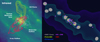 |
Fig. 1. Schematic summary of the activity within central molecular zone of NGC 253. See Sect. 1 for a comprehensive summary of the activity in its central region as probed by multiwavelength observations. In both figures, the CO traced CMZ, and the dense gas traced GMCs (Leroy et al. 2015) are included as a spatial scale reference. Left: IRAC 8μm from Spitzer Local Volume Legacy survey (Dale et al. 2009) in the background; Chandra X-ray traced outflow (Strickland et al. 2000); 18 cm OH plume (Turner 1985); molecular outflow observed in CO emission (Bolatto et al. 2013). Right: 2 cm TH sources (Turner & Ho 1985) and HII regions and supernovae remnants (Ulvestad & Antonucci 1997); proto-super stellar clusters traced by vibrationally excited HC3N emission (Rico-Villas et al. 2020); star cluster identified from near-IR HST imaging (Watson et al. 1996). |
As one of the brightest extragalactic infrared sources (Soifer et al. 1989) and the most prominent molecular emitter beyond the Magellanic Clouds, the prototypical local starburst galaxy NGC 253 has been the target of multiple molecular spectral line studies (see Table 1). Due to its proximity, high resolution studies can resolve the giant molecular cloud (GMC) scales of a few tens of parsecs (Sakamoto et al. 2011; Ando et al. 2017; Leroy et al. 2018). In particular, NGC 253 has been the target of a number of ALMA observations which analyzed the properties of individual molecular clouds and complexes within its CMZ (Sakamoto et al. 2011; Meier et al. 2015; Leroy et al. 2015, 2018; Ando et al. 2017; Mangum et al. 2019; Martín et al. 2019b; Rico-Villas et al. 2020; Krieger et al. 2020).
The ALMA Comprehensive High-resolution Extragalactic Molecular Inventory (ALCHEMI) is an ALMA large program whose aim is to obtain the most complete spatially resolved unbiased molecular inventory toward a starburst environment. For this purpose we carried out a broadband spectral scan toward the NGC 253 CMZ with a homogeneous spatial resolution. Unbiased wide-band spectral line surveys provide immediate advantages over narrow-band spectroscopy since the detection of multiple transitions per molecular species allows us to observationally constrain the excitation conditions (e.g., Aladro et al. 2011b; Pérez-Beaupuits et al. 2018; Scourfield et al. 2020). They also allow for the evaluation of line blending between molecular lines by simultaneously fitting many transitions of a given species rather than fitting individual spectral features.
The main objectives of ALCHEMI are to: (1) Define a uniform molecular template for an extragalactic starburst environment, where systematic uncertainties are minimized; (2) accurately constrain the physical conditions of individual star-bursting molecular cloud complexes; (3) study the ISM enrichment by stellar nucleosynthesis through measurement of isotopic ratios; (4) enable a direct comparison of the physical and chemical ISM properties between the Milky Way and an active star-forming environment; (5) explore the chemistry of complex organic molecules (COMs) in the CMZ of NGC 253; (6) evaluate gas processing in galactic outflows. This study provides a template for the molecular emission in a starburst galaxy that can be compared to future spatially-resolved millimeter and submillimeter studies of more distant galaxies on GMC size scales.
This paper, the first in a series of articles which will describe the scientific results from ALCHEMI, provides a global presentation of the ALCHEMI survey that includes data obtained with both the main (12 m) and Morita (ACA 7 m) arrays. However, here we focus, as a first step, on the analysis and discussion of the low resolution (15″ ∼ 255 pc) 7m array data. This study aims at describing the global molecular properties of the entire unresolved CMZ of NGC 253. As such, and similar to existing single-dish line surveys but with improved frequency coverage and sensitivity (5.6× broader and > 2 − 10 deeper than Martín et al. 2006), the low resolution data analyzed here provide a template of a starburst environment for spatially-unresolved targets at larger distances. Already at this low resolution we explore the physical conditions of the gas and the enrichment of the ISM, and peer into the genesis of complex organic molecules in NGC 253.
2. Observations
The CMZ in NGC 253 was imaged with ALMA in frequency Bands 3, 4, 6, and 7 as part of the Cycle 5 large program 2017.1.00161.L. The survey was subsequently extended to Band 5 during ALMA Cycle 6 (project code 2018.1.00162.S). A total of 101.5 h of integration time on source were acquired, 38.8 hours of which were obtained with the 12 m array.
The nominal phase center of the observations is α = 00h47m33.26s,  (ICRS). Observations were configured to cover a common rectangular area of 50″ × 20″ (850 × 340 pc) with a position angle of 65° (east of north), and a target resolution of 1″ (17 pc, see Sect. 3.2). This targeted region required a single pointing in Band 3, where the 12 m antenna primary beams range between 57″ and 68″, and Nyquist-sampled mosaic patterns of 5 to 19 pointings (from the lower frequency end of Band 4 to the upper frequency end of Band 7, respectively) with the 12 m array. The average integration time per mosaic pointing to achieve the target sensitivity (Sect. 2.2) varied from ∼2.6 h in Band 3, ∼12 min in Band 4, ∼9 min in Band 5, ∼4 min in Band 6, and ∼2.5 min in Band 7. Additional single pointing observations in a 12 m more compact configuration or 7 m array were performed to achieve a common maximum recoverable scale of 15″ across the whole survey (see Sect. 2.3).
2.1. Frequency setup
The full data set results in a rest-frequency coverage between 84.2 and 373.2 GHz, with 47 individual tunings, each composed of four 1.875 GHz spectral windows from two receiver sidebands. Table A.1 compiles the frequency coverage of the final data products per tuning and separated by receiver sideband after homogeneous processing (Sect. 3.2).
The broad frequency range of 289 GHz was continuously covered except for a few narrow regions: First, the ∼9 GHz gap between bands 3 and 4 (from 116 to 125 GHz avoiding the deep 118.75 GHz telluric oxygen line) is not observable with the ALMA receivers. Between the other receiver bands, the frequency gaps are significantly narrower: only 325 MHz around 163 GHz (bands 4–5), 250 MHz around 211.1 GHz (bands 5–6), and 225 MHz around 275.25 GHz (bands 6–7). The spectral window centered close to the 183 GHz telluric water line was observed, but the data quality was not good enough for calibration. Finally, the ∼9 GHz frequency range from 319.3 to 328.3 GHz, surrounding the 325 GHz telluric water line, was intentionally not covered, given the expected poor atmospheric transmission, to reduce the number of tunings necessary to cover the large frequency width of ALMA Band 7.
A variable frequency overlap of 50 to 500 MHz was used between two adjacent spectral windows within a given sideband, and a frequency overlap of 100–200 MHz between contiguous tunings was adopted, allowing us to check the relative amplitude calibration across the survey (Sect. 3.1).
The native spectral resolution was 0.977 MHz, equivalent to 3.4 to 0.8 km s−1 (with Hanning smoothing) for Bands 3 to 7, respectively. Only a few setups in Band 7 (B7g to B7p) had some spectral windows set to a resolution of 1.128 MHz. Final products were produced at a coarser uniform velocity resolution during imaging (Sect. 3.2).
2.2. Sensitivity
The targeted brightness temperature sensitivity of the survey was 50, 50, 40, 30, and 30 mK in 10 km s−1 channels across ALMA Bands 3, 4, 5, 6, and 7, respectively. This was a compromise to achieve a deep uniform sensitivity across all bands while keeping an achievable ALMA time request. These brightness temperature sensitivities can be converted to point source flux density sensitivities using Eq. (3.31) in the ALMA Cycle 8 technical Handbook1:
For the originally-specified circular beam size of 1″ the approximate point source flux density sensitivities are ∼0.35, 0.9, 1.2, 1.6, and 2.3 mJy at the ALMA frequency band centers.
The flux density root mean square (RMS) values of each individual continuum subtracted spectral window were estimated from line free spectral channels. Channels showing bright line emission were masked by hand, while those showing fainter emission were eliminated by using the biweight algorithm in the CASA task imstat (McMullin et al. 2007). The top panel in Fig. 2 displays the measured flux density RMS of each spectral window as a function of frequency. Combined (12 m compact plus extended configurations in Band 3 or 12-m plus 7-m array data for higher frequency bands, see Sect. 2.3) sensitivities (blue) as well as the 12-m compact configuration (green) and 7-m array (red) sensitivities are shown. Figure 2 shows that for most of the survey, the achieved flux density complies with the project’s original sensitivity goals. Apart from the spectral windows directly affected by the 183 GHz telluric water line (USB of B5b, B5c, and B5d, and LSB of B5e) and the oxygen and water lines at 368 GHz and 380 GH, respectively (USB of B7m and B7n), the flux density RMS noise ranges from 0.18 to 5.0 mJy beam−1, with average flux density sensitivity of 1.4 mJy beam−1 and median of 1.0 mJy beam−1. This noise is measured in the final 8 − 9 km s−1 channels (Sect. 3.2).
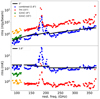 |
Fig. 2. Measured RMS flux density (top) and equivalent brightness temperature (bottom) noise level of each individual data cube (spectral windows) imaged for the combined arrays (blue), compact 12 m array band 3 observations (green) and 7 m array band 4 to 7 (red). Black lines correspond to the target sensitivities requested for 1″ (top) and |

The bottom panel in Fig. 2 displays the 1.6″ beam (Sect. 3.2) equivalent brightness temperature noise per spectral window. The targeted brightness temperature sensitivity with a beam of 1″ is corrected by a factor of 2.56 to account for the achieved common beam of 1.6″ (Sect. 3.2). The average sensitivity is 14.8 mK with a median of 10.2 mK.
2.3. Maximum recoverable scales
Due to the lack of short spacings in interferometric observations, structures larger than the maximum recoverable scale (MRS) are filtered out. Following Eq. (7.6) in the ALMA Cycle 8 technical handbook1 the MRS is defined as θMRS ∼ 0.6λ/Bmin, where λ is the wavelength and Bmin the shortest projected baseline.
Based on the extent of the CO J = 1 − 0 emission (Meier et al. 2015), ALCHEMI targeted an MRS of 15″ across its entire frequency coverage. This corresponds to spatial scales of up to ∼250 pc, which should recover most of the emission from the GMCs in the NGC 253 CMZ. These spatial scales also correspond to one fourth of the region enclosed within the ILR (Sect. 1) and are similar to the length of the 120 − 320 pc filaments tracing the molecular outflow (Bolatto et al. 2013). In Band 3, our required MRS could be achieved with the extra-compact 12-m array configuration, but additional observations with the ACA 7-m array were required for Bands 4 through 7. Figure 3 displays the MRS for each of the individual 12-m and 7-m array observations. The targeted MRS was achieved across the entire ALCHEMI spectral coverage, ensuring that ≲15″ scales are recovered throughout the survey. We note however that at the lower frequencies, scales larger than 15″ could also contribute to the observed emission. In that sense, the survey is not strictly homogeneous, although this could be corrected, if deemed important for a given science case, by cropping the visibilities within a given uv radius. Based on the results presented in Sect. 4, we expect only minor contributions from structures larger than our expected MRS of 15″, with the exception of CO transitions.
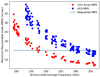 |
Fig. 3. Maximum recoverable scale per channel estimated for each individual 12-m (red) and 7-m (blue) array observations (Sect. 2.3). Each point corresponds to an individual execution centered at the average frequency of all four spectral windows (thus the gaps that appear in some frequencies). The targeted 15″ maximum recovered scale is represented by an horizontal black line. |
3. Data calibration, equalization, and imaging
Calibration and data quality assessment were performed by ALMA staff. For all but a couple of scheduling blocks the ALMA calibration pipeline was used. A summary of the calibrators used within each scheduling block is provided in Table A.2.
3.1. Flux calibration accuracy
According to the ALMA Cycle 5 Proposer’s Guide2, delivered absolute flux calibration should be better than 5% for Bands 3, 4 and 5, and 10% for Bands 6 and 7. The flux calibration method adopted by ALMA (described in Guzmán et al. 2019) uses regularly-monitored fluxes from a catalog of secondary flux calibrators to set the flux calibration scale for all science measurements. One or more secondary flux calibration sources are measured with each science scheduling block. The absolute flux scale for the secondary calibrators are determined through almost simultaneous measurements of primary flux calibrators (solar system objects, including Uranus, Neptune, Callisto, Ganymede, and Mars) with a monitor cadence of 10 − 14 days. The accuracy of this flux calibration scheme has not been fully assessed, and recent studies suggest that the ALMA flux calibration uncertainty can be significantly worse than that stated in the ALMA user guidelines (Francis et al. 2020; de Kleer et al. 2021).
Taking advantage of the multiple contiguous frequency tunings of the ALCHEMI data set across the five covered frequency bands, we are able to further estimate the relative flux calibration accuracy of the individual frequency tunings. Prior to this analysis, data were cleaned and preliminary imaging was performed to a common beam as described in Sect. 3.2. Two independent methods were used to check the relative flux alignment. We derived amplitude scaling factors between tunings (Table A.1), based on overlapping channels (Sect. 3.1.1). The relative continuum level was then used to double check the accuracy of our spectral flux alignment (Sect. 3.1.2).
For a target source with strong continuum and a significant amount of spectral line emission within each independent frequency tuning, absolute flux calibration precision is required. Accurate absolute flux calibration minimizes amplitude misalignment in the final concatenated spectrum as well as assures a high level of accuracy when comparing spectral line fluxes derived from different frequency tunings. As shown by Harada et al. (2018), for spectra with a low density of spectral lines per sampled frequency bandwidth, one can derive and subtract the continuum emission first within individual tunings. This continuum information can then be used to perform an amplitude rescaling, followed by concatenation of the continuum-subtracted spectra from each frequency tuning to achieve accurate relative flux scaling and minimal gaps at the frequency tuning boundaries. Subtraction of a smooth continuum from a spectrum with a high density of spectral lines, on the other hand, cannot extract the necessary continuum emission information in order to use this flux rescaling technique. We describe a method to improve the flux calibration accuracy of our ALCHEMI spectra when there is a high density of spectral lines in Sect. 3.1.1.
In Appendix B we show the unscaled spectra where only the standard ALMA pipeline calibration has been applied to the data. As evidenced by Figs. B.1 through B.7 and in the scaling factors in Table A.1 some of the misalignment between adjacent receiver tunings are beyond nominal calibration uncertainties. In Appendix C we provide an analysis of the relative and absolute flux calibration uncertainties for all ALCHEMI image cubes.
The two methods used below assume that flux calibration has no systematic bias, or said otherwise, cannot account for systematic biases in the fluxes accross the spectral scan. In fact, our analysis suggest that for absolute flux calibration an overall uncertainty of 15% is justified and appropriate. However, the derivation and application of the amplitude scaling factors has allowed us to improve the relative flux calibration accuracy beyond that which a single ALMA scheduling block might normally attain. The relative flux calibration scaling factors listed in Table A.1 were applied to the originally calibrated visibilities prior to final imaging. In the analysis presented in this paper (Sect. 4), only the statistical uncertainty in the fits due the noise in the spectra are considered and not the absolute flux calibration uncertainty mentioned above, which is enough for our purposes.
3.1.1. Overlapping channels alignment
As the ALCHEMI spectra toward NGC 253 in many cases possess a high degree of spectral crowding, we refined our flux calibration by using the target signal itself as reference. This technique, originally developed for other ALMA spectral scans, is referred to as “flux self-calibration” (Sakamoto et al. 2021). Below we recapitulate the technique details fully described there.
The amplitude re-scaling in this technique is based on a comparison of the initial spectra at their overlaps, which as described in Sect. 2.1 has been built-into our scheduling block tuning setup for this purpose. For the choice of the reference signal it does not matter whether the emission at that position is dominated by continuum or spectral line emission as long as it is reasonably spatially compact and presents no time variability over the observation period. This is due to the fact that a pair of frequency tunings is always compared at their overlapped frequencies, using the same emission from each frequency. Furthermore, the ALCHEMI spectra have been produced with the same spatial resolution across each spectral scan, so that the two observations being compared should possess approximately the same range of baseline uv lengths at their respective overlapped frequencies. This flux self-calibration through overlapping tunings can therefore be used on targets with numerous broad lines with a limited number of line-free channels. A single scaling factor is derived for each tuning, shared by all the spectral windows in that tuning. It is important to note that the flux scales for individual spectral windows within a given sideband align to ≲1%.
As indicated in Sect. 2.1 our frequency setup included a 100 − 200 MHz overlap among contiguous frequency tunings. In order to derive the flux rescaling factors for each frequency tuning and array configuration, we assigned to each frequency tuning a scaling factor ai, where i is the scheduling block ID (Col. 1 in Table A.1). For each set of adjacent tunings we then solved (with the least squares method when necessary) a set of equations given by:

where rij is the measured amplitude ratio between the independent frequency tunings i and j. The spectra extracted from the TH2 position (αJ2000 = 00h47m33.182s, δJ2000 = −25° 17′17.148″; Lenc & Tingay 2006) within the preliminary imaged data cubes was used as the reference measurement in Eq. (2). We used the constraint mean(ai) = 1 to set the overall scale of the solutions, resulting in the flux self-calibration rescaling factors listed in Table A.1. These flux rescaling factors were applied to the calibrated visibilities before final imaging using the CASA task gencal as follows:

where  and
and  are initial ALMA delivered and final uv amplitudes. As evidenced by the scaled spectra shown in Figs. B.1 through B.7 the rescaled spectral image cubes are in most cases well-aligned in amplitude.
3.1.2. Continuum level alignment
We can use the continuity of the spectral energy distribution of the continuum emission to verify the relative amplitude scaling of the different tunings. One advantage of this method is that it can make a bridge across bands and gaps in the frequency coverage (Sect. 2.1) which is an intrinsic uncertainty when using overlapping channels (Sect. 3.1.1). The continuum emission is measured on the STATCONT continuum cubes (Sect. 3.3), after the first amplitude scaling derived from the overlapping channels alignment process (Sect. 3.1.1). While the amplitude scaling was applied per tuning, here we measure the continuum emission for each individual spectral window. The position TH2, close to the continuum emission peak, is also used as in Sect. 3.1.1. At this step, we do not want to introduce a complicated fit of the overall SED, so we simply use a third order polynomial to estimate the standard deviation of the continuum levels with respect to a smooth and continuous function. This strategy allows us to test the robustness of the channel-overlapping scaling by checking “residual” scaling factors (i.e., if the channel-overlapping scaling was perfect across all data, then those new factors would be all equal to one).
We have run this method on both the 7m-array and 12m+7m array cubes separately. After removing a few spectral windows close to the 183-GHz telluric water line (in Band 5), which appear as clear outliers, we find that the standard deviation of the new scaling factors is 2.5% across all bands, for both 12m+7m and 7m array data. We can thus take this value as the maximum additional error after the channel-overlapping scaling, since the STATCONT cubes may introduce some uncertainty due to line crowding and imperfect continuum estimation. Alternatively, this result suggests that the continuum determination is relatively robust and uniform over spectral windows. We note that the dispersion increases slightly toward the highest frequency edge for the 7m-array data, as the RMS of the new scaling factors for Band 7 alone goes to 3.5%.
3.2. Imaging
Before imaging, several homogenization corrections were applied to all ALCHEMI data sets in order to produce a uniform science archive. In addition to the normalization of the amplitude scale in each tuning using the procedure described in Sect. 3.1.1, all measurement sets were binned to a common velocity scale. A common velocity scaling was produced by binning to frequency resolutions of 3, 5, 6, 8, and 10 MHz for Bands 3, 4, 5, 6, and 7, respectively, which is equivalent to an approximately common velocity resolution of ∼8 − 9 km s−1 in the LSRK velocity reference frame. Once homogeneity in amplitude scaling and velocity resolution was attained, the CASA task tclean was used to produce image cubes of each tuning spectral windows. The specific tclean parameters used for imaging were catered to the needs of individual spectral windows as follows.
The cell and image sizes used for imaging each array and frequency band were as follows: 7m Array observations used cell = 0.4 arcsec and imsize = [320, 320] pixels for all frequency bands; 12m Array and the combined 7m+12m data sets used cell = 0.15 arcsec for all frequency bands and imsize=[800,800], [800,720], [720,648], [640,512], and [640,512] for Bands 3 through 7, respectively. Automasking was used for clean region selection
Based on tclean dry-runs of the ALCHEMI measurements containing known strong spectral features (i.e. CO 2 − 1), a list of line-free spectral channel RMS values for those spectral windows was developed to use as input for the tclean parameter threshold. This was necessary to allow for the proper cleaning of spectral windows where strong spectral lines amplify imaging artifacts, causing the single channel noise values near strong spectral lines to be anomalously high. For spectral windows which contained strong spectral lines, the predetermined spectral channel RMS values were used to set the tclean threshold, leaving the nsigma parameter unset. For spectral windows which did not contain strong spectral lines, the tclean parameter nsigma=2 was set, and the threshold parameter was left unset. Spectral channel flagging was performed on those spectral windows which contained clear absorption due to telluric oxygen and water (see Sect. 2.1).
The hogbom deconvolver function was used for all spectral windows. The mosaic gridder was used for spectral windows comprised of multiple pointings, while the cube gridder was used for Band 3 and all ACA spectral windows as these measurements required only a single pointing (Sect. 2). Robust (Briggs) weighting was used with a robust parameter of 0.5 for most spectral windows. In order to produce images with resultant spatial resolution of 1.6″, a few tunings required alternate robust parameters for each of the four spectral windows, and in three cases uv range settings: B3b used robust = [0.4, 0.5, 0.5, 0.5]; B3c used robust = [0.25, 0.5, 0.5, 0.5]; B3f used robuts = [0.0, 0.0, 0.5, 0.5]; B5d used robust = [0.0, −2.0, 0.5, 0.5] and uvrange > 20 kλ; B5e used robust = [ − 2.0, −2.0, −2.0, −2.0] and uvrange > 25 kλ; B5f used robust = [ − 2.0, −2.0, −2.0, −2.0] and uvrange > 50 kλ.
The originally requested angular resolution was 1″ (17 pc). However, the synthesized beams of each individual spectral window significantly varied between frequency setups and between individual spectral windows in the upper and lower sidebands due to the effective antenna configuration used for each observation. This fact did not allow the imaging of the entire survey at the targeted spatial resolution. In order to produce a homogeneous data set, with data cubes sharing a uniform spatial (and spectral) resolution over all frequencies, a common final spatial resolution of 1.6″ (28 pc) was selected, corresponding to that of the data cube with the coarsest resolution in the survey. Post-imaging convolution using the CASA task imsmooth was therefore performed to produce final image cubes with a fixed Gaussian circular beam of 1.6″.
Additional data cubes were generated for the compact 12-m array observations at Band 3 and the 7-m array observations for Bands 4 through 7. Data were imaged with a common restoring beam of 4″ and 15″, respectively, for these two compact array configurations.
3.3. Continuum subtraction
It was determined that it would be inefficient to subtract the continuum in the uv plane from the individual 188 data cubes constituting the ALCHEMI measurement set. The large velocity gradient across the field of view and the significant cumulative line contribution even in the low resolution data (Sect. 4.2) makes it difficult to accurately identify line free windows to perform the continuum subtraction in the uv plane for all data cubes. Therefore, for consistency across the entire survey, continuum emission was statistically derived from each individual spectral window using STATCONT (Sánchez-Monge et al. 2018) to derive and subtract the continuum on a per pixel basis from each image cube. Sigma-clipping continuum determination was used with the default parameter (α = 1.8, see Sánchez-Monge et al. 2018, for details).
Continuum subtraction was performed on both the initial input data cubes used to feed the flux level alignment and also on the final amplitude-scaled data (Sect. 3.1). The per-pixel continuum estimation was thoroughly tested and provides good overall results. Since the algorithm was mostly tuned to confusion limited Galactic sources with relatively narrow spectral line emission, we observe that the continuum appears slightly overestimated in the regions of spectra with higher noise levels. For example, the continuum level appears to be overestimated near the 183 GHz telluric water line and at the upper end of Band 7 (> 335 GHz). More importantly, continuum subtraction is seen not to be optimal for spectral lines close to the noise level. In such cases, continuum subtraction in the uv plane or subtraction of a spectral baseline in the image plane using a narrow window around the lines of interest may be needed for accurate imaging.
3.4. Self-calibration
It is foreseen that the ALCHEMI data set will eventually be improved with self-calibration of both the ACA and 12m Array measurements. However, the data in this article and the data that will initially be publicly released from this ALMA large program will not include self-calibration. The ALCHEMI research collaboration intends on providing a subsequent version of the ALCHEMI image cube archive which includes the application of self-calibration. It is important to note that self-calibration may have an impact on the absolute flux calibration of the ALCHEMI measurements. As a result, we emphasize that the amplitude scaling factors derived in Sect. 3.1 will need to be recalculated after self-calibration of the ALCHEMI data.
4. ACA data: Analysis and first results
While Sect. 2 describes the observational details of the full ALCHEMI survey, here we focus on the ACA 7-m (Morita) array alone. The ACA data allow us to probe the global properties of the molecular emission of the CMZ in NGC 253. This provides a template for subsequent analysis of the high resolution data to compare molecular abundances on individual GMC size scales to those on the larger size scales probed by the ACA.
The frequency coverage of the ACA data in this analysis is limited to the 256.7 GHz surveyed with this array; ALMA Bands 4 to 7 between 125.2 and 373.2 GHz. Figure 4 presents an overview of the survey. As indicated in Sect. 3.2, a homogeneous reconstructing beam of 15″ was used across the entire frequency range. This resolution is roughly equivalent to that of the 2 mm (i.e., ALMA Band 4) spectral survey in Martín et al. (2006) carried out with the IRAM 30-m single-dish telescope. However, in contrast to single-pointing surveys with single-dish telescopes for which the resolution changes as a function of frequency, our ACA interferometric observations allow for uniform spatial resolution across the entire frequency coverage.
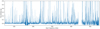 |
Fig. 4. Full spectral coverage obtained with the ALMA Compact Array (ACA 7m) alone, extracted from the position of brightest molecular emission (see Sect. 4.3.1). Figure F.1 presents a zoomed version of this plot in five frequency windows 50 GHz wide where the comparison with the modeled emission (Sect. 4.3.2) and the molecular line identification of each individual feature is included. Figures F.2–F.11 present a further zoomed version in 5 GHz windows. |
The point-source flux density sensitivity of the ACA data alone (Fig. 2, top) is lower than that of the combined data presented in Sect. 2. If we exclude the noisy data sets at the highest frequencies (i.e., USB of B7m and B7n), sensitivities range between 1.8 and 19.4 mJy beam−1 across the survey, with an average RMS of 7.8 mJy beam−1 and a median of 7.5 mJy beam−1. For the 15″ synthesized beam, using Eq. (1), those values correspond to equivalent point-source brightness temperatures between 0.27 and 1.0 mK, and an average of 0.6 mK.
4.1. Continuum emission
Having continuous frequency coverage over ∼260 GHz ranging from 2 mm to 850 μm (resulting in Δν/ν ≃ 1 at the central frequency of the survey) allows us to study the spatially averaged continuum spectral energy distribution (SED). This frequency range is particularly interesting because we can probe the Rayleigh-Jeans (RJ) tail of the dust emission as well as the free-free continuum emission from ionized gas and, to a lesser degree, synchrotron emission from nonthermal sources in the CMZ of NGC 253.
Continuum emission is barely resolved at our 15″ resolution as derived from the two sample STATCONT continuum product images at 198 and 350 GHz. The 2D Gaussian fit to both continuum images yields a similar 18″ × 14″ (FWHM; PA = 55°) emission extent which hints at some elongation along the major axis of the CMZ. In Fig. 5, we show the continuum emission as derived from STATCONT (Sect. 3.3) for each spectral window at the pixel position analyzed in this article (Sect. 4.3.1). Although this is not strictly an SED (νFν vs. log(ν)) we will refer as such in the following. Due to the slightly extended emission compared to our spatial resolution, if the continuum is measured integrating over an aperture larger than the beam instead of using the continuum value at the emission peak, a similar SED shape is obtained but with 15 − 20% larger flux densities. The SED was calculated from amplitude-aligned data cubes on overlapping channels (Sect. 3.1.1). Thus, the SED is spectrally smooth except for the regions in which the spectra are noise dominated such that STATCONT did not accurately fit the continuum (Sect. 3.3). Such is the case with the apparent drop in continuum intensity due to the higher noise in the measurements around the telluric 183 GHz H2O transition in Fig. 5.
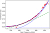 |
Fig. 5. Continuum flux density at the peak of emission as derived from each spectral window across the surveyed frequency range (red dots). We note that extended emission in our data might account for up to ∼20% higher fluxes (Sect. 4.1). A fit to the data is shown by a continuous blue line, which is the combination of the free-free emission (dotted blue almost horizontal line) and the graybody emission (dashed blue line). See text for further details on parameters used. As a reference to illustrate the deviation from pure black body emission, that for a Td = 50 K and 0.5″ source size is shown as a green dot-dashed line. |
The observed curvature of the continuum SED in Fig. 5 fits well to a graybody with dust temperature Td = 42 ± 1 K, mass Md = 8.0 ± 0.2 × 10⁵ M⊙, emissivity β = 1.9 (i.e., S ∝ ν3.9), and a mass opacity coefficient of dust, κν = κ0(ν/ν0)β, where κ0 = 0.1 cm2 g−1 and ν0 = 250 GHz (e.g., Cao et al. 2019), plus a free-free component to account for the lower frequency emission with SFR = 2.5 M⊙ yr−1 and Te = 104 K (S ∝ ν−0.1, using Eq. (3) in De Zotti et al. 2019).
The dust temperature was fit to the data in Fig. 5 using Herschel observations (with no aperture correction applied) at high frequencies, finding good agreement with the cold component fit of 37 K by Pérez-Beaupuits et al. (2018). Similarly the derived mass agrees well with the Pérez-Beaupuits et al. (2018) value of 1 × 10⁶ M⊙ if we correct our estimate to account for the extra 20% flux from extended emission in our data (see above). The higher temperature components derived by Pérez-Beaupuits et al. (2018) are negligible at our observed frequencies. Dust emissivity (β = 1.9) based on this data agrees well with that derived by Rodríguez-Rico et al. (2006).
Synchrotron emission was also included in the fit shown in Fig. 5 based on Eq. (1) in De Zotti et al. (2019) which considers a steepening of the emission above 20 GHz. Since we assumed a SFR = 2.5 M⊙ yr−1 the synchrotron emission at our observed frequencies is negligible compared to that due to free-free emission. However, our assumed SFR is slightly higher than that derived from radio recombination lines (∼1.7 M⊙ yr−1: Kepley et al. 2011; Bendo et al. 2015) or the SFR of ∼1.7 M⊙ yr−1 derived from a fit to the free-free emission by Rodríguez-Rico et al. (2006). The power law emission resulting from the combination of synchrotron and free-free emission can only be disentangled with observations at lower frequencies not covered by the ACA data in this article.
4.2. Line contribution to broadband continuum emission
Observations with broad, coarse spectral resolution mm and submm continuum detectors such as bolometers may suffer from contamination by spectral line emission. The 40-GHz-wide spectral scan at 1.3 mm toward the ULIRG Arp 220, reported a line contribution to the total observed flux of ∼28% (Martín et al. 2011). The wide spectral coverage ALCHEMI data set allows us to investigate the typical line contamination for a starburst galaxy like NGC 253. In order to obtain the spectral line contribution to the total emission per frequency band, we calculated the average flux density over the continuum subtracted spectrum and divided it by the observed average flux density (continuum plus line emission) over the same band. Results are shown in 5 GHz bins in Fig. 6 and averaged over 50 GHz bands in Table 2.
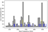 |
Fig. 6. Spectral line contribution to the continuum flux in 5 GHz bins. The position of spectral features brighter than 1 Jy are shown as blue segments at their corresponding frequency, with the two CO J = 2 − 1 and 3 − 2 transitions displayed in yellow. |
Line contribution to the observed flux density.
Similar to the results for Arp 220, we observe a significant contribution from spectral lines to the continuum-integrated flux density in NGC 253. Most of the contamination is due to the brightest lines in the band, as shown by color segments in Fig. 6, but there is also a significant contribution from the forest of weaker lines. The line contribution, both in narrow 5 GHz and broad 50 GHz bins, ranges from a few percent up to a third of the measured flux density, and up to 80% in narrow ranges containing CO transitions. We note that the CO contribution over the 50 GHz band considered in Table 2 would account for 8% in both Bands 6 and 7, similar to what was reported toward Arp 220 (Martín et al. 2011), while the remaining contribution of up to ∼35% corresponds to emission from other species.
Both this work and that on Arp 220 can now serve as a reference for evaluating the line contribution to broadband continuum observations (i.e., with too coarse spectral resolution to resolve the lines) and considering corrections to broad continuum observations over ALMA Bands 3 to 7 (rest frame), and correspondingly to the spectral index derived from those measurements. Such corrections may be particularly relevant for high-redshift galaxies showing a nuclear starburst contribution.
4.3. Molecular emission analysis
4.3.1. Selected sample position
In order to analyze the global molecular emission of the CMZ in NGC 253, we targeted the peak of the molecular emission in the 15″ resolution data. To select this position, the pixel of peak emission was measured for each of the moment 0 maps from 16 of the brightest transitions in the survey shown in Fig. 7. The spectra analyzed in this article were extracted from the pixel at position  ,
,  , corresponding to the average of all measured peak emission pixels and shown as a blue cross in Fig. 7. This position is just ∼1.5″ away from the giant molecular cloud analog Region 5 from Leroy et al. (2015) and ∼1.4″ from TH2 (Turner & Ho 1985).
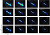 |
Fig. 7. Sample of integrated flux density moment 0 maps from 16 of the brightest molecular transitions in the covered frequency band. Each panel is labeled with the corresponding molecular species and transition. We point out that CO 1 − 0 is not included since Band 3 is not covered by the ACA data. In color the combined 12 m+7 m maps are shown where the color coding is adjusted for visibility of each individual species. Gray contours show the 7 m integrated intensity images where the n-th contour level corresponds to 20 n3 Jy km s−1 beam−1 for all species. Species are ordered in decreasing order of integrated flux density from left to right and from top to bottom. The panel in the lower left shows the reference coordinates and the beam size of the combined 12 m+7 m ( |

We note that despite the different spatial distribution among species observed at the high resolution data, the brightest pixel in these ACA images agrees well among all images. Peak positions deviate from the average of all peak positions within an RMS of 0.8″ (∼2 pixels), and/or within 0.65″ (∼1.5 pixels) if we exclude the two CO transitions, whose emission structure is significantly affected by opacity and overall extended emission.
4.3.2. Line identification and LTE modeling
In this section we describe the overall criteria for molecular line identification and modeling. Further specific details on the fitting of individual species are provided in Appendix D. We emphasize that we did not analyze individual spectral features, but modeled the emission of all spectral lines within the surveyed band at once for each species. Therefore, line identification is done per molecule and not per transition, which is more robust and makes use of the broad frequency coverage in this work. Line flux densities reported in this paper are those from fits to the molecule transitions and accounts for line blending. We do not report the measured flux of each individual spectral feature.
Molecular emission has been identified and modeled under local thermodynamic equilibrium (LTE) conditions using MADCUBA3 (Martín et al. 2019a) where physical parameters of column density, excitation temperature, radial velocity, line width, and source size are used to fit a modeled synthetic spectrum to the observations. Spectroscopic parameters required for LTE modeling in MADCUBA, and therefore all the frequencies reported in this paper, are extracted from the CDMS (Müller et al. 2001, 2005; Endres et al. 2016) and JPL (Pickett et al. 1998) catalogs.
One of the visual advantages from fitting through synthetic spectra is that non-LTE emission or just spectral lines not properly fit under the LTE assumption are evidenced by line intensities significantly deviating from the LTE fit, which is often overlooked in the log-log representation in rotational diagrams. As explained in Appendix D, the LTE approximation appears to work well to describe the vast majority of observed spectral features modeled in this analysis, and the most obvious deviations from the fit are also identified.
The spectra extracted at the selected position (Sect. 4.3.1) show a double peak profile which is the result of the convolution of the molecular distribution substructure observed at higher resolution (see Fig. 7). In principle, fitting a two component model would allow us to kinematically disentangle the molecular gas from both sides of the nucleus. However, the use of a multiple Gaussian fit to the overall spectrum adds little significance to the results (which will be better studied with the high resolution ALCHEMI image cubes), while increasing significantly the complexity of the modeling, even more so given that not all species show double peak profiles. For these reasons the modeling described here will consider a single Gaussian emission profile which suits the purpose of this article’s focus on the global averaged properties of the molecular emission in the CMZ of NGC 253.
Among the fitted parameters, fitting the source size requires an accurate “a priori” excitation temperature for a molecule with enough optically thick transitions covering a wide range of energy levels and not too affected by spectral blending (Martín et al. 2019a). Since the broad line emission in our spectrum does not allow for an accurate constraint of the source size, we assumed a circular Gaussian equivalent source size of 5″, based on available higher resolution observations (Meier et al. 2015; Martín et al. 2019b). This parameter is not too relevant for the global relative properties analyzed in this article, as we consider a linear dependence of the derived column density with the source solid angle. It could, however, be significant for lower values of the source size, when opacity starts playing a major role as discussed in Sect. 5.4. Only in the case of the main 12C16O isotopologue did we find it necessary to assume a larger source size of 10″ to be able to reproduce the observed flux densities. A difference in the larger molecular emission extent is obvious from the contours in Fig. 7 for the CO transitions, and to a lesser extent the 13CO images.
All other physical parameters mentioned above (column density, temperature, velocity, and width) were kept as free parameters when possible. For each molecule, all available transitions within the covered frequency band were used for the fit, except those heavily blended or not detected above the noise level (< 3σ). In some cases, for species with many transitions, only a subset of the brightest unblended transitions were used to avoid the fit being dominated by faint transitions too close to the noise level or residual emission from other species. When line blending or signal-to-noise did not allow fitting the line velocity and width, parameters were fixed to vLSR = 230 km s−1 and Δv1/2 = 150 km s−1, which are the average fitted parameters to the brighter transitions. Similarly, when detected transitions did not allow the excitation temperature to be determined, the excitation temperature was set to Tex = 15 K, which is the median of the measured temperatures in all species allowing such a fit (ranging between 5 and 60 K). Additionally, whenever any of these parameters (with the exception of the column density) were derived from a given species, these values were used to obtain more appropriate parameters to be fixed in the fit to their rarer isotopologues or isomers. This allows for a better relative abundance comparison between related species, while no biases resulting from this assumption are obvious in our derived values.
The final model includes 146 species with a total of 42121 transitions. However, only 78 species are considered firmly or tentatively detected, accounting for 1790 transitions with flux densities above 2 mJy in the model. We note that 2 mJy corresponds to 1σ at the lowest frequencies and ∼(1/3)σ for the majority of the survey. However, the sum of faint transitions (even below the noise level) is relevant since in some cases they add up to detectable features or may significantly contaminate other transitions. The detected molecule count includes isotopologues and vibrational states. In addition multiple hydrogen and helium recombination lines from Hnα, Hnβ, and Henα were also detected throughout the survey but are not discussed in this article.
The criterium for detection of a given species has been based on its LTE model and fit results. A species has been considered detected if all the detectable transitions above 5σ (according to the LTE model), which are not blended with brighter transitions, are detected in our data. Additionally we required the convergence of the fitting algorithm within MADCUBA to avoid subjective biases.
Table A.3 shows the result from the fit to all detected or tentatively detected species in this survey. As previously indicated in Sect. 3.1, reported uncertainties do not include calibration uncertainties but statistical uncertainty on the fit to the spectra. Values with no errors in Table A.3 represent parameters that were fixed during the fitting process.
Figure 8 shows a graphical summary of the number count in flux density bins and in narrow 5 GHz frequency bins of the transitions in the model. Table 2 also includes the density of spectral lines over wider 50 GHz frequency ranges.
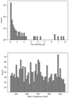 |
Fig. 8. Top: histogram showing the number of spectral lines above 2 mJy in the model in bins of flux density. Lines between 2 mJy and 10 Jy are considered. The three spectral features with flux densities above 10 Jy are not included in this diagram. Bottom: histogram showing the number of spectral lines above 2 mJy in frequency bins of ∼5 GHz width. |
Finally, we point out that there are still a number of clearly detected spectral features which are not accounted for by our model as seen in the figures in Appendix F. These unidentified features may stem from emission out of LTE or the effect of multiple molecular components (Aladro et al. 2011b) or from species not included in our model. We evaluated each of these features for emission from different species, but a model to the candidate species could not be found to fit across the whole frequency range covered.
4.4. New extragalactic molecular detections
Despite the moderate sensitivity of the ACA observations, the broad frequency coverage and the bandpass stability allowed us to probe a number of newly detected species in the extragalactic ISM.
In this paper we report the first extragalactic detections of H CO, ethanol (C2H5OH), 13CCH, C13CH, HOCN, the three 13C isotopologues of CH3CCH, propynal (HC3HO), and tentatively Si17O (see discussion in Sect. 5.4.2). Specific details on the fit to C2H5OH, HOCN, and HC3HO are provided in Appendix D.1. Additionally, we confirm previous tentative detections of H15NC (Muller et al. 2006), 13CH3OH (tentatively detected toward NGC 253 by Martín et al. 2009a, and recently reported toward PKS1830-211 by Muller et al. 2021), and HC5N (Aladro et al. 2015; Costagliola et al. 2015). These detections consist of isotopologues and isomers of previously detected species, as well as new complex organic molecules (COMs, 6+ atoms, Herbst & van Dishoeck 2009). Species like formic acid (HCOOH), very recently reported toward an absorption system (Tercero et al. 2020), is detected for the first time in emission toward NGC 253. We also confirm the detection of the elusive methylamine (CH3NH2, Bøgelund et al. 2019), first detected in the extragalactic ISM in absorption by Muller et al. (2011) and so far only tentatively identified toward NGC 253 in emission by Meier et al. (2015).
The chronological evolution of the cumulative number of species detected as well as the yearly detections are summarized in Fig. 9, where the detections reported in our work are included. Details on the updated chronology of first extragalactic molecular detections are provided in Appendix E.
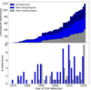 |
Fig. 9. Chronology of extragalactic molecular detections including those reported in this work. Detections of main and rarer isotopologue substitutions in blue and gray respectively, with the total number of detections, not considering tentative reports, being displayed in dark blue. One and two year bins are used for top and bottom panel histograms, respectively. |
5. Discussion: NGC 253 as starburst molecular template
Even with its moderate angular resolution, the ACA data set provides important information on the abundance and excitation of the gas in the CMZ of NGC 253, which could not be attained by previous surveys with less complete frequency coverage (Martín et al. 2006; Aladro et al. 2015). In this section, we highlight some scientific results that make use of the wide frequency coverage of the ALCHEMI data. This unique frequency coverage allows for multitransition analysis of a variety of molecular species. The upcoming suite of papers based on ALCHEMI data will also make use of this unique wide band data set and will provide a deeper analysis of these and other scientific questions.
5.1. Extragalactic starburst low resolution molecular template
One immediate use of the wideband observations in this article is to serve as a molecular template for extragalactic starbursting environments. The large number of molecules detected in this study is a consequence of both the depth of the ALCHEMI data set and the intrinsic brightness of NGC 253. In fact, we obtained a spectral dynamic range between ∼60 000 and ∼6000, as derived by comparing the flux density of the brightest transition in the survey, CO 3 − 2 (see Table A.3), to the ACA-achieved noise level at Bands 4 and 7 (Sect. 4), respectively.
Figure 10 presents the number of detected unique species as a function of the flux level relative to the CO 3 − 2 transition (left panel) or to the brightest transition within a given Band (right panel). The data presented in Fig. 10 are based on modeled intensities from individual transitions and not spectral features (Sect. 4.3.2). Therefore the number count of species is conservative, since spectral features composed of multiple transitions (e.g., species with unresolved hyperfine structure) will rise above the noise before what is estimated based on the flux density of the brightest transition of any given moleucule. The number of detected species in Fig. 10 goes beyond the number of confirmed detections reported in Sect. 4.3.2. This is because the number of species in Fig. 10 includes recombination lines and species in vibrational states, as they are both considered to be relevant unique detections.
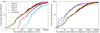 |
Fig. 10. Number of individual detectable species as a function of the flux density level relative to the brighter transitions detected in the survey per band. Left: flux density levels are referred to the CO 3 − 2 (112 Jy beam−1) as the brightest transition detected in the whole spectral range covered. Right: flux densities are referred to the brightest transition detected on each band. This is CS 3 − 2 (0.9 Jy beam−1 in Band 4), HCO+ 2 − 1 (3 Jy beam−1 in Band 5), CO 2 − 1 (56 Jy beam−1 in Band 6), and CO 3 − 2 (in Band 7). |
The data presented in Fig. 10 can be used to roughly estimate the expected level of molecular complexity achievable in a high redshift “starbursting” object as a function of the sensitivity of the observations. Of course, the main assumption relies on similar abundance and excitation conditions to those in NGC 253, which may not hold for all starburst environments (Aladro et al. 2015). Additionally, larger line widths would hamper the detectability of species due to blending.
As a test bed to show the template potential of our data set we used the stacked spectrum derived from 22 high-z sources by Spilker et al. (2014), over the redshift range z = 2.0 − 5.7, and covering the frequency range from ∼250 to 800 GHz. Based on their Fig. 2, the CO 3 − 2 line was detected at a signal-to-noise of ∼50. That is, observations should be able to detect emission lines ∼17x fainter if we impose a 3σ detection level. Based on our Fig. 10 (left), if we consider lines ∼17 times fainter than CO 3 − 2 (the level could be even lower considering the integrated line intensity) would result in a detection of 3-4 species. Spilker et al. (2014) reported six species above 3 σ. However, based on the mid panel in their Fig. 2, only three spectral features actually reach the 3σ level at the spectral resolution in their diagram. The increased noise in the small fraction of rest-frame Band 6 they covered resulted in no detections, also in agreement with what would be expected based on the NGC 253 template. Considering a factor of two lower sensitivity in this region, only CO 2 − 1 would be expected, and its frequency was actually not covered in their observations. This comparison shows the predicting potential of NGC 253 for molecular detections toward high-z starbursting galaxies.
5.2. Vibrational emission
Rotational transitions in vibrational states (hereafter vibrational emission or transitions) of HCN, HNC, and HC3N, with lower energy levels of 1000, 700, and 500 K above the ground state, respectively, are clearly detected in the ACA data analyzed in this article. Vibrational emission toward NGC 253 has been recently reported at subarcsecond resolution toward individual GMCs with observations of the J = 4 − 3, v2 = 1f transitions of HNC and HCN (Ando et al. 2017; Mangum et al. 2019; Krieger et al. 2020), and two rotational transitions in multiple vibrational states of HC3N (Rico-Villas et al. 2020). However, it was never detected in low resolution spectral scans of NGC 253 (Martín et al. 2006; Aladro et al. 2015), with spatial resolution similar to that in this work. While HC3N emission in the v7 = 1, v7 = 2, and v6 = 1 states is clearly detected at  resolution (Rico-Villas et al. 2020), we only detect significant emission from v7 = 1 states. We attribute this difference to beam dilution of the vibrational emission which originates from the compact GMC cores (Rico-Villas et al. 2020, 2021; Krieger et al. 2020). This is similar to what is observed within our Galaxy where vibrational emission is solely arising from hot dense material within star forming cores (de Vicente et al. 2000; Martín-Pintado et al. 2005).
The wide-band imaging of ALCHEMI data allows us to probe multiple vibrationally excited transitions of these species and to evaluate the contamination by other species. Figure 11 shows the rotational transitions of HCN, HNC, and HCO+ in the v2 = 1f vibrational state. Transitions in the v2 = 1e state are too close in frequency to the rotational transitions in the ground vibrational state (see Fig. 3 in Martín et al. 2016). The derived LTE fit to the emission of all observed transitions assumes an excitation temperature Tex = 300 K required to make these high energy transitions detectable (red line in Fig. 11). This fit clearly shows that the LTE approximation does not properly reproduce the excitation of these radiatively pumped transitions (Aalto et al. 2015). Table 3 presents the line ratio between the observed rotational transitions in the ground vibrational (v2 = 0) and v2 = 1f vibrational states. As previously reported, the relative intensities between rotational transitions within a vibrational state follow that measured within the v = 0 rotational transitions (Costagliola et al. 2015; Rico-Villas et al. 2020), with v2 = 0/v2 = 1f ratios relatively constant. We note that fitted column density is not physically meaningful since it requires full radiative transfer modeling to take radiative pumping into account.
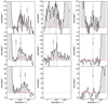 |
Fig. 11. Rotational transitions in the vibrational state v2 = 1f of HCN, HNC and HCO+ covered within the surveyed frequency range. The box corresponding to HNC 2 − 1 v2 = 1f was left intentionally blank since its emission at 182.6 GHz falls within the telluric water transition observation gap (Sect. 2). Red lines show an attempt to fit the observed emission under LTE assuming Tex = 300 K (see text in Sect. 5.2 for details). Nearby transitions from detected species with modeled flux densities > 10% of that of the vibrational transitions are labeled. |
Spectral line emission properties of the vibrational transitions of HCN, HNC, and HCO+.
Based on the analysis of the full spectrum we estimate that the transitions presented in Fig. 11 are only marginally blended with fainter transitions from other species, with the exception of HCN J = 2 − 1 v2 = 1f and more importantly HNC J = 4 − 3 v2 = 1f. Although not blended with other species, HCO+J = 4 − 3 v = 2f falls between two bright features and we therefore consider this line to be tentatively detected. The other two HCO+v = 2f transitions, J = 3 − 2 and 2 − 1, are not detected as shown in Fig. 11.
5.2.1. High temperature driven “carbon-rich” chemistry
Our data show that the vibrational emission of HCO+ is one order of magnitude fainter both relative to the observed emission of vibrational HCN and HNC as well as relative to the HCO+ ground vibrational state (see Table 3). The detection of the J = 4 − 3, v2 = 1f transition alone might be considered tentative but still relatively faint compared to the corresponding transitions of HCN and HNC. However, if the same ratio among J transitions within the vibrational level of HCN and HNC would apply to HCO+, we would then expect the 3 − 2 and 2 − 1 transitions to be significantly above the LTE fit in Fig. 11. Since this is not observed, we argue against the detection of vibrationally excited HCO+.
The wavelengths of photons required to excite the vibrational states range from ∼22 μm for HNC to 12 − 14 μm for HCN and HCO+ (Aalto et al. 2007; Sakamoto et al. 2010; Imanishi et al. 2017; González-Alfonso & Sakamoto 2019). High column densities and dust temperatures are required for the effective photon trapping leading the vibrational excitation of these molecules (González-Alfonso & Sakamoto 2019). However, the differences in the conditions for IR pumping of these species may explain the different relative intensities to their respective ground vibrational transitions (Sakamoto et al. 2010). For instance, the one order of magnitude larger HNC Einstein coefficient make it easier to pump than HCN (Aalto et al. 2007). However, these excitation differences alone do not explain the non detection of vibrational HCO+ which has relatively similar excitation conditions to HCN.
Detections of vibrational transitions of HCN, HNC, HC3N, and seemingly CH3CN have been reported toward an ever increasing number of (U)LIRGs (see the compilation by Falstad et al. 2019) at the frequencies covered by ALCHEMI. However, beside the recent detections of vibrationally excited HCO+ in absorption toward the gas-poor AGN in NGC 1052 (Kameno et al. 2020) and the faint emission feature (relative to the global galaxy emission) toward the molecular torus around the luminous AGN in NGC 1068 (Imanishi et al. 2020), no detections of HCO+ in vibrational states have been reported in extragalactic environments.
Similar to what is reported here toward NGC 253, an explicit nondetection of vibrational HCO+ emission was reported toward the compact LIRG NGC 4418 and the ULIRG IRAS 20551-4250 (Sakamoto et al. 2010; Imanishi et al. 2017), while clearly detecting HCN and/or HNC vibrational emission. Imanishi et al. (2017) claimed an overabundance of HCN toward IRAS 20551-4250, following the statistically suggested higher rotational emission HCN/HCO+ ratio in AGN dominated environments (Izumi et al. 2013; Privon et al. 2015; Imanishi et al. 2016). However, as suggested by Izumi et al. (2013) based on the chemical modeling of Harada et al. (2010) high temperature chemistry could be responsible for such a relative HCN overabundance.
At high temperature (Harada et al. 2010), a “carbon-rich” chemistry can be mimicked when oxygen is locked in the form of H2O. In such conditions, carbon bearing species such as HCN and HNC may be boosted by 1–2 orders of magnitude, while HCO+ would be reduced by a similar amount. This may actually be the scenario in hot dense gas around the protostars in starburst dominated environments. In these regions high temperatures and densities are required not only to drive the efficient infrared pumping of vibrational states (Td > 100 K, Aalto et al. 2015) but also to populate transitions such as those of HC3N to J = 40 − 39, with critical density ncrit ∼ 107 cm−3 and lower level energy El ∼ 350 K (Wernli et al. 2007). Within the ALCHEMI measurements, observed intensities above the LTE-derived fit to HC3N indicate the presence of a high excitation temperature component.
The proposed scenario, in which high temperatures drive “carbon-rich” chemistry, would be supported by the nondetection of vibrationally excited oxygen-bearing species such as HCO+, while the rotational transitions in the ground vibrational state, not originating in the denser infrared pumped region, may appear to be as bright as those of HCN and HNC. Similarly it would explain the relatively rich complex carbon chain chemistry detected in NGC 253 (Sect. 5.3), as well as the high abundances of HC3N and HC5N not only in NGC 253 (Aladro et al. 2015) but also in the prominent compact obscured nuclei (CON) in the ULIRG Arp 220 and the LIRG NGC 4418 (Martín et al. 2011; Costagliola et al. 2015), two well known emitters of vibrationally excited rotational lines. The locking of oxygen into H2O would also explain the bright emission of H2O and its weaker isotopologue H O reported toward Arp 220 (Martín et al. 2011; König et al. 2017). Furthermore, the “carbon-rich” scenario might also be supported by bright HCN relative to CO emission reported toward the molecular outflow in Arp 220 (Barcos-Muñoz et al. 2018), where the oxygen depleted hot dense gas might have been blown away by the nuclear activity (due to either a starburst or active galactic nuclei).
5.2.2. Vibrational emission as tracer of global proto-SSC contribution
The ratios between the vibrational emission and the infrared luminosity for HCN, HNC, and HCO+ are summarized in Table 3. The ratios measured with HCN J = 3 − 2, v2 = 1f are about an order of magnitude below the Lvib/LIR = 10−8 threshold defining the extreme compact obscured nuclei, such as the above mentioned NGC 4418 and Arp 220 (Falstad et al. 2019).
We compare NGC 253 CMZ global average Lvib/LIR = 1.4 × 10⁻⁸ derived from HCN J = 3 − 2, v2 = 1f with that of 4.2 × 10⁻⁸ measured toward the Galactic Center hot core Sgr B2(N) at a spatial resolution of 0.1 − 1.2 pc (Rolffs et al. 2011). Assuming that vibrational emission is mostly contributed by Sgr B2(N)-like hot cores, this comparison results in a ∼3% level as a proxy to the contribution from proto-SSCs to the global infrared luminosity in NGC 253. In fact, this estimate is consistent with the contribution from proto-SSCs of ∼3% derived by Rico-Villas et al. (2020) based on high resolution imaging of vibrationally excited HC3N toward NGC 253. We note that Rico-Villas et al. (2020) used a 25% lower IR luminosity from the CMZ of 1.6 × 10¹⁰ L⊙, but still both results remain in good agreement.
Thus, we tentatively show that vibrational emission could be used as a 0th-order proxy to the proto-SSC contribution to the total infrared luminosity in extragalactic environments, under the assumption that there is marginal or no vibrational emission contribution by AGN heating as recently suggested from observations of the Seyfert galaxy NGC 1068 (Rico-Villas et al. 2021; Imanishi et al. 2020).
5.3. Organic molecules
As described in Sect. 4.4 some of the newly detected species in NGC 253 are organic molecules. In the following we briefly discuss the measured abundances of ethanol (C2H5OH) and formic acid (HCOOH). These species are selected as ancillary comparison data exists from Galactic Center molecular clouds to provide an initial comparison of organic species abundances toward NGC 253; while we leave further more comprehensive discussions on organic molecules to upcoming publications using the higher resolution data. The detection of these organic species can only be unambiguously claimed thanks to the large spectral coverage which has allowed us to properly account for line blending and to cover multiple transitions from these large molecules.
Based on a sample of Galactic Center (GC) GMCs Requena-Torres et al. (2006) claimed an apparently homogeneous COM composition across the Galactic central molecular zone. In their study, the comparison between Galactic hot cores and GMCs showed that organic abundances relative to methanol, and in particular those of C2H5OH and HCOOH, agree within a factor of two, although the abundances toward hot cores were systematically found on the high end of the measurements (Fig. 12). The detection of these two species over CMZ scales toward NGC 253, allows us to include, for the first time, an extragalactic environment into this comparison. This allows us to explore the claimed grain composition homogeneity outside our Galaxy, and in this case toward a star-bursting environment.
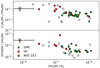 |
Fig. 12. Abundances of C2H5OH and HCOOH relative to CH3OH toward the NGC 253 CMZ (orange star), compared to those measured toward Galactic hot cores (red squares; Ikeda et al. 2001) and Galactic Center giant molecular clouds (green circles; Requena-Torres et al. 2006). Upper limits to C2H5OH and HCOOH are represented by open symbols. |
Figure 12 places the abundances of C2H5OH (1.1 ± 0.4 × 10⁻¹) and HCOOH (2.8 ± 1.0 × 10⁻²) relative to CH3OH toward NGC 253 in the context of the Galactic Center GMCs observed by Requena-Torres et al. (2006) and the Galactic hot cores from Ikeda et al. (2001). Relative abundances with respect to methanol are commonly used to explore relative COM abundances while avoiding uncertainties associated with an estimate of H2 column densities. In our analysis we have estimated the methanol abundance relative to H2 from C18O and assuming 18O/16O = 100 (as derived in Sect. 5.4.2) and CO/H2 ∼ 8 × 10⁻⁵ (Frerking et al. 1982), which yields NH2 = 3.1 × 1023 cm−2, in good agreement with previous single dish observations after correcting for the different assumed emission extent (Martín et al. 2009b). We included a conservative factor of two uncertainty in the H2 determination to account for uncertainty in these assumptions. As expected, the relative abundance of CH3OH in NGC 253 is significantly lower than in Galactic Center sources, since the clumpier methanol emission is referred to the global extended H2 emission traced by CO over the large scales probed in our low resolution observations. Therefore the CH3OH/H2 in Fig. 12 can be actually considered a lower limit.
The comparison in Fig. 12 shows that the averaged abundances toward NGC 253 are on the high end of GMC measurements, similar to what is observed in the sample of hot cores. In particular the abundance of HCOOH is among the highest in the sample, but still a factor of three below the observed one in the Sgr B2(N) hot core (Requena-Torres et al. 2006).
Within the Galactic Center, emission from complex organic molecules is clearly detected toward hot molecular cores associated with massive star formation (e.g., Belloche et al. 2013, 2017, 2019). However, early surveys on a sample of GC GMCs (Requena-Torres et al. 2006, 2008; Martín et al. 2008a) and the recent reports of an ever increasing COMs richness in GC quiescent clouds (Zeng et al. 2018; Rivilla et al. 2019, 2020; Bizzocchi et al. 2020; Jiménez-Serra et al. 2020) are evidence of the widespread COM emission over GMC scales.
Previous single dish line surveys toward the CMZ of NGC 253 claimed that the observed average chemical abundances resemble that of GC GMCs (Martín et al. 2006; Aladro et al. 2011a). This chemistry would be mostly driven by the widespread large-scale shocks affecting its CMZ (García-Burillo et al. 2000; Martín 2009; Meier et al. 2015). Indeed, these widespread shocks in NGC 253 would be the responsible for the global ejection of organic molecules from dust grains into the gas phase, similar to what is observed within the Galactic CMZ (Martin-Pintado et al. 1997; Martín et al. 2008b).
Our low resolution observations show how the emission from organic species described above, although consistent with that in GMCs, might imply a significant contribution from hot-core emission based on the observed abundances relative to methanol being closer to those found in GC hot cores. Such a hot core contribution should be significant since it is detectable in the averaged low resolution spectrum in this starbursting environment. The actual distribution and resolved abundances across the CMZ in NGC 253 will be better analyzed with the high resolution ALCHEMI data which will allow the comparison between the individual NGC 253 GMCs and the Galactic Center quiescent GMCs and hot cores.
5.4. Isotopic ratios
Investigating the elemental isotopic ratios and the difficulties to measure them with different molecular proxies in nearby galaxies is key to extend these studies to more distant objects, as well as probing the evolution of isotopic enrichment through cosmic time (Muller et al. 2006; Wallström et al. 2016; Kobayashi et al. 2020). A major advantage of the wide frequency coverage of the ALCHEMI survey is to allow for the measurement of isotopic ratios based on all the molecular isotopologue pairs detected within the covered bands, coupled with the relatively accurate column density measurement based on multiple transitions observed at the same angular resolution. The use of individual species and/or single transitions are subject to potential uncertainties in opacity (see Sect. 5.5), excitation, blending effects, as well as chemical fractionation.
Table 4 shows the isotopic ratios derived from the column densities fitted to all detected isotopologue pairs (Sect. 4.3.2). This table is graphically represented in Fig. 13 where the equivalent range of values measured in the Milky Way are also displayed for comparison. As explained in Sect. 4.3.2, a source size of 5″ was used for all species except for CO where a size of 10″ was required to match the observed absolute flux density of the CO transitions. In order to provide a meaningful ratio of CO isotopologues when referred to the main isotopologue, the emission of 13CO and C18O fits were recalculated for an equivalent source size of 10″. In this way the ratio is meaningful, despite opacity considerations, since all the CO isotopologues present resolved structure in the low resolution maps (Fig. 7). We observe how the carbon and oxygen ratios derived with the main CO isotopologue are consistently a factor of 2 − 10 below those measured with any other isotopologue pairs in Table 4 (Sects. 5.4.1 and 5.4.2). This is evidence of the opacity affecting CO even in the averaged CMZ emission.
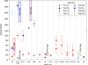 |
Fig. 13. Measured NGC 253 isotope ratios in the ACA data (Table 4) compared to their equivalent values in the Milky Way (Wilson 1999). The horizontal axis indicates the molecular species, or in the case of CO the isotopomer, used to measure a given isotope ratio. Colored rectangles are used to indicate Milky Way isotope ratio value ranges. As no uncertainties nor range of values was provided for the Si isotope ratios, a range of 10% of the estimated values was assumed. As the Milky Way 16O/17O value would be ≳875, we have opted to not show this Milky Way isotope ratio value. |
Column density ratios in the CMZ of NGC 253 based on the ACA data.
The values in Table 4 are optical depth corrected, under the assumptions of LTE and similar source extent. When it was possible to fit the excitation temperatures in the different isotopologues of a given species, we found a good agreement (Sect. 4.3.2). For the assumed source size of 5″ most of the main isotopologues show moderate optical depths (≲1), so column density ratios are close to the optically thin regime and therefore close to what would be derived from line intensity ratios. The advantage of using column density ratios is that we are considering the contribution from all transitions of a given molecule, rather than relying on a single transition.
In order to evaluate the effect of the assumed source size on the opacity of the main isotopologue and, consequently on the derived isotopic ratio, Table 5 shows the LTE fit results for various assumed source sizes, where HCO+ is selected as case example. We note that for sizes < 3″, increasing the excitation temperature Tex is requierd to reproduce the observed absolute flux densities, which results in lower opacities, but it then becomes difficult to fit the emission with a single temperature component. Therefore, the ranges explored in Table 5 are a good representation of the effect of opacity on the derived isotopic ratio, which can become a factor of two larger than the optically thin approximation.
Effect of source size on the 12C/13C ratio derived from HCO+.
To put our results into context, Table 6 compiles all isotopic ratios reported in the literature toward NGC 253. The “nominal” isotopic ratios commonly used in the literature for local galaxies, as compiled in Wilson (1999), are 12C/13C = 40, 16O/18O = 200, and 18O/17O = 8. However, these derived values are subject to the limitations of the species used as proxy as well as the uncertainty of the opacity in the brighter isotopologue (see Sect.5.5 for a discussion on opacity). Placing our NGC 253 observations into context of previous detections is key since these standard isotopic ratios are mostly based on measurements toward M 82, the other prototypical nearby starburst galaxy, and our target NGC 253 (see overview and discussions in Henkel et al. 2014; Martín et al. 2019b; Tang et al. 2019)
Integrated intensity isotopic ratios toward NGC 253 in the literature.
In the following we discuss individual atomic ratios which are probed by our molecular column density ratios and are globally averaged over the CMZ in NGC 253 at our ACA resolution.
5.4.1. Carbon
Observations within the center of our Galaxy show the dependency of the observed isotopic ratios on the molecular species used as proxy. Such variations are observed in 12C/13C using H2CO, CO, and CN isotopologues (Gardner & Whiteoak 1982; Langer & Penzias 1990; Milam et al. 2005). In fact, recent chemical models predict different 12C/13C ratios for different molecular species depending on the density, on the chemical formation pathways, the temperature and on the cosmic-ray ionization rate (Colzi et al. 2020; Loison et al. 2020; Viti et al. 2020). Therefore, variations among species are expected as they can also trace different gas components.
Under the assumptions described in Sect. 5.4 and excluding the values derived from CO isotopologues (see below), our observations show column density derived 12C/13C ratios ranging from 17 to 60, with an error weighted average ∼25 ± 10. The largest values are derived from the isotopologues with the faintest transitions, close to the noise level and more affected by the uncertainties due to blending to other species. Therefore, the uncertainties in the ratios may be significantly higher than the pure statistical uncertainty from the fit. Still, they are included in Table 4 for the sake of completeness. The weighted average taking into account only the ratios with the lowest uncertainties, that is the brighter species, namely HCO+, HCN, HNC, CN, CS, and H2CO, is 22 ± 2. This value is just marginally lower than the weighted average considering all species and in much narrower agreement among them as can be graphically seen in Fig. 13.
The low average ratio observed in the brighter species of 22 ± 2 is in good agreement to previous low resolution observations (see Table 6 and notes therein), which were used to derive the nominal extragalactic ratio of 40 based on opacity considerations. In fact, the only way to reconcile the average 12C/13C ratio with the literature value of 12C/13C∼40 is by assuming a smaller source size (see discussion in Sect. 5.4) where the emitting gas within this 850 × 340 pc region is actually confined to a region of ≲5″ (≲85 pc). This would imply that all the brightest species showing ratios around ∼20 in Table 4 would be affected by approximately the same optical depth. However, based on the opacity of the brightest transition of these species (Table 4), we do not expect the same opacity effect on all these species, and it would not be supported by the discussion of the opacity of sulfur species (Sect. 5.4.4).
We note that, CN/13CN observations by Tang et al. (2019) derived opacity corrected ratios ranging 30 − 67, and at a similar angular resolution a value of 21 was derived from C18O/13C18O by Martín et al. (2019b). This discrepancy cannot be explained by opacity effects (see Sect. 5.5), but rather by tracing a different molecular component. Despite the uncertainty on the fainter isotopologues, the ratios derived from CCH isotopologue pairs (Fig. 14) are consistent with the limit of > 50 derived at single dish resolution based on the non detection of both C13CH and the 13CCH by Martín et al. (2010).
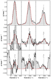 |
Fig. 14. Spectral features of the J = 4 − 3 (left), 3 − 2 (center) and 2 − 1 (right) transitions from three of the isotopologues of CCH detected in the survey. Red curves shows the LTE model best fits. Contributions by other species is almost negligible for most transitions according to the global LTE model from the full survey (see Sect. 4.3.2). However we note that the observed profile of 13CCH 4−3, not following the CCH LTE model and not accounted for by emission from other species, was not used in the fit. |
The ratios estimated based on CO isotopologues appear to be significantly different than those from higher dipole moment species. As mentioned in Sect. 5.4, the lower value derived from CO/13CO is the result of a large opacity affecting the CO main isotopologue, so this value is not considered meaningful.
Now focusing on the rarer CO isotopologue pairs, our averaged 12C/13C ratio based on higher dipole moment species agrees well with the value of ∼21 ± 6 derived at 3″ resolution using the C18O/13C18O column density ratio (Martín et al. 2019b). In their work, they concluded that there was no obvious signature of high optical depth in the measured 3 mm transitions of the rarer CO isotopologues. However, our measured C18O/13C18O ratio in the 15″ resolution data in this work is a factor of four above the ratio measured with other species and to that measured with the same isotopologue pair at 3″ resolution by Martín et al. (2019b). On the other hand this ratio agrees with the limit of > 60 estimated from single dish observations at 23″ resolution (Martín et al. 2010). This high ratio is clearly apparent in the spectral features shown in Fig. 15. We note, for completeness, that both the single dish and high resolution measurements referred here use the J = 1 − 0 transitions. In principle this should not cause differences in the ratios if both transitions originate from the same regions and share similar excitation conditions. As pointed out by Martín et al. (2019b), the different ratios measured at high and low resolution might be evidence for the existence of two distinct components with different degrees of stellar nucleosynthesis ISM processing, similar to what is observed in the Galactic Center (Riquelme et al. 2010). As indicated by Viti et al. (2020), the difficulties to reproduce such a high value from chemical modeling is evidence of the large range of carbon isotopic ratios measured being the result of nucleosynthesis and not fractionation.
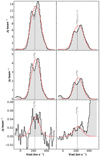 |
Fig. 15. Spectral features of the J = 3 − 2 (left) and 2 − 1 (right) transitions from three of the rarer isotopologues of carbon monoxide detected in the survey. Red curves show the LTE model best fits. Contributions by other species are not shown since all features appear to be free of contamination. |
In this multicomponent scenario, the low resolution observations would be tracing extended unprocessed material with a 12C/13C ratio of ∼100, similar to what is observed in the outskirts of our Galaxy (Wouterloot & Brand 1996). This material must have recently been driven toward the nucleus from the outer regions by the stellar bar in NGC 253 (Sect. 1) and not yet enriched by ongoing star formation in the CMZ. On the other hand, the denser and more compact gas dominating the GMC emission would be enriched by the starburst event (e.g., Romano et al. 2017) resulting in 12C/13C ratios of ∼20 − 30 as traced by optically thicker high electric dipole moment molecules even at low resolution. The high resolution observations of the optically thinner CO transitions would also trace this processed molecular gas with 12C/13C ratio of ∼21 (Martín et al. 2019b).
Tracing the more extended, potentially less processed gas by CO isotopologues agrees with them being the only transitions showing extended emission at the ACA resolution (Fig. 7). Although selective photodissociation might play a more important role in 13C18O, this effect should also affect C18O and to a lesser extent 13CO. We note that despite the uncertainty due to the noise, 13C18O line profiles match very well those of the more abundant CO isotopologues (Fig. 15).
5.4.2. Oxygen
The situation with oxygen ratios is consistent with that encountered with carbon ratio measurements. Our 16O/18O ratio of 100 ± 20 measured with HCO+ could be reconciled with the value in the literature of 200 if we account for a possible multiplicative factor of two due to opacity as discussed above. The value derived with the main CO isotopologue is half (48 ± 5) of that derived with HCO+, once again due to the high opacity of CO (Sect. 5.4). However, that derived with the 13C substitutions of CO results in a ratio of 520 ± 60 which, similar to the carbon isotopic ratio discussed above, is a factor of five above that measured with HCO+, but still within the range of values observed within the Milky Way as displayed in Fig. 13. The 16O/18O ratio is in reasonable agreement with previous single dish measurements (69, Aladro et al. 2015) and in good agreement with the value measured at higher resolution with the 13C substitutions of CO (130, Martín et al. 2019b) as shown in Table 6.
The scenario depicted by the oxygen ratios would be similar to that from carbon isotopic ratios with a low 18O enriched material traced by the optically thin rarer CO isotopologues. Regarding 17O, we find good agreement between our measured 18O/17O∼9 ratio and the range derived from single dish measurements (7 − 10). The 16O/17O ∼ 400 derived with the main CO isotopologue, similar to the values derived toward individual GMCs by Meier et al. (2015), would translate into an actual value of ∼800 based on the differences observed between CO derived ratios and those with other species above. Finally the low 16O/17O ∼ 13 value deduced from SiO sheds doubts on the actual detection of Si17O unless its flux density is boosted due to non-LTE effects, in which case the ratio measured would not be indicative of the actual oxygen ratio. We therefore report its detection as tentative.
5.4.3. Nitrogen
Chemical modeling of nitrogen isotopic ratios has recently been published by Viti et al. (2019), where models are compared with existing measurements in the extragalactic ISM. Here we present the first 15N isotopologue detection toward NGC 253 and we place it in the context of previous observations toward other galaxies and high-redshift molecular absorbers. The 14N/15N nitrogen isotopic ratio measured with both HCN (147 ± 15) and HNC (220 ± 50) are consistent with a weighted average of 170 ± 20. This value is also in agreement with the 14N/15N∼152 ± 27 measured toward the molecular absorber PKS 1830-211 (Muller et al. 2011) and with the 14N/15N∼227 ± 41 of toward NGC 4945 (Henkel et al. 2018). In both objects, the HNC ratio is higher, but significantly more uncertain, than that measured with HCN.
The H13CN/HC15N ratio of 5.6 ± 0.6 is close to that measured toward PKS 1830-211 (4.8 ± 0.2) and almost twice that of the other molecular absorber B 0218+357 of 3.0 ± 0.5 (Wallström et al. 2016). This ratio is 35% lower than that measured toward NGC 4945 at ∼40 pc resolution (2″, Henkel et al. 2018), where they find a global value of ∼8.5 ± 1.7, although values of 4 − 6 are measured outside the very nuclear region, in contrast with the value of 2.1 ± 0.3 at 60″ resolution toward the same object (Wang et al. 2004). On the other hand the ratio HN13C/H15NC of 13 ± 3 is about twice that measured toward PKS 1830-211 of ∼7 (Muller et al. 2011).
Similar to what is discussed with the other isotopic ratios, the effect of opacity could raise the 14N/15N ratio up to 400 if the opacity correction suggested in the carbon isotopic ratio discussion is considered. Based on the updated 14N/15N galactocentric trend by Colzi et al. (2018), a value of 400 would correspond to a 8 kpc galactocentric distance, while the 4 kpc molecular ring shows a ratio of ∼300, which decreases 200 at ∼1 kpc. The latter is consistent with the value derived here, uncorrected for putative high opacity.
We note that the non detected spectral features of both N15NH+ and NN15H+ down to our achieved noise level is in agreement with the derived 14N/15N.
5.4.4. Sulfur
32S/34S ratios measured with both CS and SO (9.7 ± 0.5 and 14 ± 4, respectively) are in good agreement with previous single-dish measurements based on CS observations of 8 ± 2 (Martín et al. 2005) and more than a factor of two above that derived from SO (5.1 ± 1.2 Martín et al. 2006). However, the latter is likely the result of uncertain de-blending from SO2 emission on a very faint feature (see Appendix C.4 in Martín et al. 2006)
However, if the CS emission is actually optically thick, in order to reconcile the carbon isotopic ratios with the nominal extragalactic value of 40 (see Sect. 5.4), then the main CS and SO isotopologues should show the same peak optical depth. This way, the derived 32S/34S would be similar in both species. Based on the fit values in Table A.3, the opacity ratio between both species is measured to be τC34S/34SO ∼ 15 which does not support the idea of CS being optically thick, unless both species are tracing very different sulfur isotopic ratio components.
Our sulfur isotopic ratio of 32S/34S ∼ 10 is about half of the Galactic Center value of ∼22 measured with 13CS/C34S (assuming a 12C/13C) or ∼17, directly obtained from 13CS/13C34S (Frerking et al. 1980; Wilson & Rood 1994; Humire et al. 2020). However, taking into account the 32S/34S Galactocentric gradient reported by Yu et al. (2020), there is a good agreement with the trend value within the Galactic central kiloparsec.
Our measured 13CS/C34S = 0.42 ± 0.04 is in between the average value measured in Galactic disk sources and sources in the Galactic Center region (between 0.35 and 0.68 Frerking et al. 1980).
Although as discussed above we do not see evidence for opacity effects in the sulfur isotopologue ratios, both opacity uncorrected and corrected values would lie within the range of values observed in other extragalactic sources (see, e.g., Wallström et al. 2016).
5.4.5. Silicon
Here we derive the first silicon isotopic ratios measured in emission toward external galaxies through the observed ration between SiO and the rarer 29SiO, 30SiO, and Si17O substitutions.
The ratios presented in Table 4 yields 29Si/30Si∼4.2, which is more than a factor of two above the value of 1.5 within the Galaxy (Penzias 1981; Anders & Grevesse 1989; Lodders 2003), and the value of 1.9 measured toward PKS 1830-211 (Muller et al. 2013). The apparent overabundance of 29Si might imply that this is not a primary nucleus but resulting from some stellar processing. However, observations of silicon isotopic ratios toward a wider variety of environments are required to further analyze the origin of silicon isotopologues, since there appears to be no difference between solar and Galactic Center observations (Wilson 1999).
On the other hand, the ratio 28Si/29Si = 9 ± 2 is however consistent with the ratio of 11 measured toward the molecular absorber PKS 1830-211 (Muller et al. 2011) and about a factor of two below the Solar system value of 19.6 (Anders & Grevesse 1989; Lodders 2003).
5.4.6. Isotopologue ratio overview
In this section we provide an overview of the results obtained from the different isotopologue ratios measured in this work, which are graphically summarized in Fig. 13.
Carbon, oxygen, nitrogen, and sulfur ratios measured with the brightest species other than CO, namely HCO+, HCN, HNC, CN, CS, and H2CO, are on the low end of the range measured in the Milky Way. In fact, the isotopologue ratios toward the NGC 253 CMZ are consistent with the values observed within the Galactic CMZ. These high dipole moment species may be tracing molecular gas enriched by the starburst present in the CMZ, which leads to an enrichment in the rarer isotologues, similar to what is derived from the Galactocentric trends observed in the Milky Way Galaxy (Wilson 1999; Milam et al. 2005; Yu et al. 2020). The emission from these less-abundant species appear unresolved in the 15″ resolution ACA data (Fig. 7).
Carbon and oxygen isotopic ratios measured with CO appear to have a dependency on the probed scales. The 3″ resolution ratios measured with the rarer CO isotopologues yielded reported ratios similar to those measured for the high dipole moment species in this work (Martín et al. 2019b). However, the ACA data discussed here, recovering larger scales, yields carbon and oxygen ratios consistent within the limits derived with single-dish observations (Martín et al. 2010), that is a factor of five larger than those measured at higher resolution. Carbon monoxide may be tracing a more extended molecular component not yet involved in and enriched by the star formation burst within the CMZ. Indeed, CO and its isotopologues are the only species showing extendend emission at the ACA resolution (Fig. 7). This dependence on the size scales measured highlights the importance of tracing the molecular emission at all scales, and in particular the importance of analyzing the ACA data which probes the largest molecular spatial scales.
Although opacity considerations may result in ratios which differ by up to a factor of ∼2 from the higher dipole moment species, in line with the ratios commonly found in the literature, this would imply that all species are affected by the same optical depth correction. Moreover, the high resolution study of CO isotopologues (Martín et al. 2019b), resulting in similar ratios to those from high dipole moment species as mentioned above, did not show evidences of optical depth effects except for potentially toward one of the brightest GMCs. Based on the analysis of CN emission in Sect. 5.5, it is likely that the emission from all species contains an optically thick component surrounded by an optically thin envelope within the individual GMCs.
Fractionation is considered to be negligible under the physical conditions in the bulk of the gas in galaxies (Romano et al. 2017). However, some species in our work might be showing some hints of fractionation. This appears to be the case for CCH (Table 4 and Fig. 14), where differences are found between the two 13C isomers. The relationship of ratios is not consistent with what is observed in dark clouds where CCH/13CCH > CCH/C13CH (Sakai et al. 2010). Our results also do not show evidence of the HC3N isotopologue abundance differences that are measured in low-mass star forming regions (e.g., Araki et al. 2016). The uncertainty on the abundance ratios of isotopologue substitution of these more complex species have a relatively large uncertainty, which makes it also difficult to claim fractionation in CH3CCH. Therefore we leave the discussion on the actual effect of fractionation in NGC 253 to a subsequent publication on the of individual GMCs within the NGC 253 CMZ measured at higher spatial resolution.
5.5. Opacity analysis with multitransition CN observations
One of the main sources of uncertainties in estimating column densities of the emitting molecules, or equivalently relative abundances, is the unknown effect of optical depth (Mangum & Shirley 2015; Martín et al. 2019a). Although the MADCUBA fit accounts for the effect of opacity (Sect. 4.3.2), the opacity (linearly related to the column density) and source size are partially degenerate (see discussion in Sect. 5.4). However, some molecular species present hyperfine structure transitions which are separated enough to constrain the opacity based on either the spectral feature profile or the ratio between the different groups of hyperfine spectral features. Such is the case of species like CN and CCH. In this section we analyze the hyperfine structure of multiple CN and CCH transitions, making use of the wide frequency coverage of the ALCHEMI data set. Through this analysis we highlight the importance of multitransition observations for an accurate opacity determination.
Previous studies, both at single dish resolution (Henkel et al. 2014) and ALMA high-resolution observations Tang et al. 2019), made use of the CN N = 1 − 0 hyperfine split spectral line, consisting of two groups, the  and the
  to estimate the optical depth of this transition. Within the frequency coverage of the ACA data presented in this article, we observe the N = 3 − 2 and N = 2 − 1, each consisting of three groups of hyperfine transitions as shown in Fig. 16. The brighter transitions of these groups, for reference, emit at 340.248 and 226.874 GHz, respectively. Here we present the analysis of these profiles using three simple LTE models (Fig. 16) to explain their observed emission and to estimate the optical depth affecting these lines.
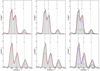 |
Fig. 16. CN N = 3 − 2 (top) and N = 2 − 1 (bottom) emission measured with the ACA data presented in this article. Panels are centered at 340.248 and 226.874 GHz, which is the frequency of the stronger emission hyperfine transition. The data are fitted with three simple models. Left: single component corresponding to the fit presented in Sect. 4.3.2, where a source size θs = 5″ is assumed. The central opacity of the brightest transitions are τ3 − 2 = 0.25 and τ2 − 1 = 0.44, while the cumulative opacity of the stronger hyperfine groups are |


Figure 16 (left panels) shows how the single component optically thin fit used in this work (for a source size of 5″) cannot reproduce the intensity of the fainter hyperfine groups, namely the  and
and  for the N = J = 3 − 2 and N = 2 − 1 groups, respectively. On the other hand, the two brighter hyperfine groups would have appeared to fit well to the optically thin regime if not considering the third group of transitions.
As a second approach (Fig. 16 center panels), we assumed a smaller (2.5″) and therefore thicker emission which accounts better for the fainter hyperfine groups. However, it does not manage to properly reproduce the emission from the two brighter groups. The three N = 3 − 2 line component groups could be considered reasonably fit within the model uncertainties if we would only be observing at this frequency. However, it clearly underestimates the emission of the brighter N = 2 − 1 group.
Finally, the right panels in Fig. 16 show a third simple model that considers two components. The model consists of one optically thin component with a 5″ source size, together with a much smaller (1.5″) optically thick component. The model fits well all three hyperfine groups in both CN transitions. In this model, the second component, ∼10× larger in mass and accounting for just ∼25% of the integrated line emission, would consist of a comb of saturated line profiles for the brighter hyperfine groups. Since the emission is saturated, the fit is degenerate and therefore the mass contained in this component (column density) is subject to a large uncertainty.
This exercise shows that, as we know from high resolution observations (Tang et al. 2019) the integrated emission of NGC 253 is a convolution of molecular components with different degrees of obscuration. Indeed, our unresolved observations point to the presence of a heavily obscured compact emitting region, very likely associated with the GMC dense cores in the NGC 253 CMZ (Sakamoto et al. 2011; Leroy et al. 2015; Rico-Villas et al. 2020) which might contain a large fraction of the mass, surrounded by a thinner likely more widespread component.
In the following we analyze the effect of such differences in size and opacities on the 3 mm transition used in the literature. By extrapolating the first two models above (left and center in Fig. 16) to the band 3 N = 1 − 0 hyperfine groups used in the literature, we obtain integrated flux density ratios between the  and
and  hyperfine groups of 1.95 (θ = 5″ optically thin model) and 1.8 (θ = 2.5″ optically thick model). Thus, the two models differ only by 8% in observed integrated intensity ratio of the N = 1 − 0 hyperfine groups. Therefore, this transition is less sensitive to optical depth effects than the combination of the two transitions consisting of three hyperfine groups observed in the ALCHEMI survey.
On the other hand CCH does not show evidence of the existence of such an optically thick component. However, the CCH hyperfine structure is not as well separated as in CN, and only the 2 − 1 and 3 − 2 groups at 174.7 and 262.0 GHz show an asymmetric profile at lower velocity due to this hyperfine structure. Unfortunately the large line width at this coarse spatial resolution together with the blending with other species, does not allow us to perform an analysis on CCH as detailed as on CN with the ACA data.
6. Summary and conclusions
The central molecular zone of the starburst galaxy NGC 253 is a complicated but interesting multicomponent system with various heating mechanisms playing a role at different scales. Previous low-resolution single-dish observations of NGC 253 showed that the averaged molecular abundances toward its CMZ resembles that of Galactic GMCs, and its observable chemistry would be mostly driven by low-velocity cloud-cloud collisions (García-Burillo et al. 2000; Martín et al. 2006).
The ALCHEMI spectral survey of NGC 253 brings new insights into the chemical composition and physical conditions of the CMZ of NGC 253. In this article we present the ALCHEMI survey covering the spectral range from 84.2 to 372 GHz. Our large frequency coverage allows us to accurately align the flux scale of the individual tunings, where we observed significant deviations. Here we present the analysis of a subset of the ALCHEMI survey, consisting of the ACA observations covering the 256.7 GHz wide frequency band (i.e., full ALMA Bands 4 to 7) between 125.2 and 373.2 GHz down to a sensitivity of 0.27 to 1.0 mK. Even at the moderate resolution of the ACA observations (15″ ∼ 255 pc) we observe a rich molecular complexity. Here we summarize the main conclusions from our analysis of the ALCHEMI ACA data.
Continuum emission in the Rayleigh-Jeans tail can be modeled with a 42 K dust emission temperature with emissivity β = 1.9 plus a free-free component with SFR = 2.5 M⊙ yr−1. This SFR is an upper limit since we cannot determine the contribution due to synchrotron emission with the frequencies analyzed in this work.
The line contribution to the observed continuum emission varies across the bands between 5 and 36% when splitting the survey into five 50 GHz frequency bins. Continuum flux emission in high-z sources with a potentially significant starburst contribution might need to be corrected in certain frequency ranges according to our findings.
Spectral line identification was performed through LTE modeling per molecule, and not per spectral feature. 78 molecular species, including isotopologues and vibrational states are detected. Additionally, multiple emission features from radio recombination lines, namely Hnα, Hnβ and Henα, are identified throughout the survey.
Newly detected species in the extragalactic ISM include complex organic species and isotopologues, namely H CO, ethanol (C2H5OH), 13CCH, C13CH, HOCN, the three 13C isotopologues of CH3CCH, propynal (HC3HO), and tentatively Si17O.
The ALCHEMI survey also provides a useful template for observations of high-redshift galaxies that can be used to estimate the number of individual molecular species that are potentially detectable in a starburst environment as a function of the depth of the observations. Our estimate is based on the stacked spectrum from 22 high-z sources at z = 2.0 − 5.7 by Spilker et al. (2014) yields 3 − 4 expected species detections, in agreement with their reported identification.
Emission from infrared-pumped vibrational states of HCN, HNC, and HC3N is detected for the first time in low resolution observations. However we do not detect vibrational emission of HCO+, similar to what is reported toward the ULIRG IRAS 20551-4250 (Imanishi et al. 2017). We postulate the existence of a “carbon-rich” chemistry as result of oxygen depletion into H2O according to high-temperature chemistry models (Harada et al. 2010). This explains both the rich carbon chemistry observed as well as the apparent lack of emission from vibrationally excited HCO+. This would be similar to what is observed in local ULIRGs, where high abundances of carbon chains (HC3N and HC5N Martín et al. 2011; Costagliola et al. 2015; Aladro et al. 2015) and water (Martín et al. 2011; König et al. 2017) are reported, as well as HCN rich outflows (Barcos-Muñoz et al. 2018).
The global averaged Lvib/LIR ratio that we measure of 1.4 × 10⁻⁹ (from HCN 3 − 2) in NGC 253 is an order of magnitude below what is observed in compact obscured nuclei (Falstad et al. 2019). We propose that this ratio is a good proxy of the proto-stellar cluster contribution to the infrared luminosity. Based on this ratio we estimate the vibrational emission originating in Sgr B2(N) like hot cores would contribute 3% to the total infrared luminosity of NGC 253, in agreement with previous estimates by Rico-Villas et al. (2020).
Organic molecules, in particular C2H5OH and HCOOH, show relative abundances consistent with those found in Galactic Center GMCs, but on the high end, similar to those measured in Galactic hot cores. Although complex organic molecules are observed to be widespread within the Galactic Center, the global abundances in the central starburst environment in NGC 253 may be significantly contributed by hot core chemistry.
We report the measurement of isotopic ratios of carbon, oxygen, nitrogen, sulfur, silicon with all the isotopologue pairs detected in our survey. 14N/15N = 170 ± 20 is measured for the first time in NGC 253. 28Si/29Si = 9 ± 2 and 29Si/30Si = 4.2 are measured for the first time in emission in the extragalactic ISM. Based on the analysis of all these ratios, we do not find evidence for opacity effects globally affecting the derived isotopic ratios.
High dipole moment species, namely HCO+, HCN, HNC, CN, CS, and H2CO, show consistent isotopic ratios of 12C/13C = 24 ± 8 and 16O/18O = 100 ± 20 which is half the standard extragalactic values (Wilson 1999) and consistent with the ratios observed within the central kiloparsec of our Galaxy. Nitrogen and sulfur isotopic ratios of 14N/15N = 170 ± 20 and 32S/34S ∼ 10 are also consistent with those in the Galactic CMZ.
Carbon and oxygen isotopic ratios derived from the rarer CO isotopologues result in values a factor of five larger than those measured with high dipole moment species and with the same CO isotopologues observed at higher spatial resolution. This result appears to confirm the multicomponent scenario where CO would be tracing the widespread gas recently funneled toward the CMZ from the galactic outskirts and therefore not yet processed by the prominent nuclear star formation. In this scenario higher dipole moment species would trace more compact dense gas clumps in the GMCs already enriched in secondary isotopologues.
Multitransition analysis of the hyperfine structure of CN reveals the presence of a likely saturated molecular component which could account for a significant fraction of the molecular mass and which is likely associated with the optically thick cores of GMCs.
The forthcoming series of papers based on the high resolution ALCHEMI data set will further investigate each of the topics presented in this paper to peer into the physical conditions that drive the observed averaged molecular abundances. The results in this article are therefore a reference for low linear resolution molecular observations of distant extragalactic sources and for follow-up studies of NGC 253 with higher angular resolution.
MADCUBA VERSION 6.0 (07/05/2018). https://www.cab.inta-csic.es/madcuba/index.html
Analysis and diagrams in these appendices make extensive use of astropy (Astropy Collaboration et al. 2013, 2018).
By array configuration we mean to differentiate among the Compact Array, either ACA (7m) or 12m Compact (12mC), the Extended Array (12m/12mE) and Combined (12m7m/12mE12mC) that were used for each spectral setup. Each of these observations consisted of a number of individual observations with slightly varying array configurations depending on the antenna availability at the time of the observation.
Acknowledgments
The authors want to specially thank David Fernández from the JAO ALMA Education and Public Outreach department for his contribution in creating the visuals presented in Fig. 1. This paper makes use of the following ALMA data: ADS/JAO.ALMA#2017.1.00161.L and ADS/JAO.ALMA#2018.1.00162.S. ALMA is a partnership of ESO (representing its member states), NSF (USA) and NINS (Japan), together with NRC (Canada), MOST and ASIAA (Taiwan), and KASI (Republic of Korea), in cooperation with the Republic of Chile. The Joint ALMA Observatory is operated by ESO, AUI/NRAO and NAOJ. The National Radio Astronomy Observatory is a facility of the National Science Foundation operated under cooperative agreement by Associated Universities Inc. N.H. is supported by JSPS KAKENHI Grant Number JP21K03634. K.S. is supported by MOST grants 108-2112-M-001-015 and 109-2112-M-001-020. L. C. acknowledges financial support from the Spanish State Research Agency (AEI) through the project No. ESP2017-86582-C4-1-R. L.C. and V.M.R. acknowledge support from the Comunidad de Madrid through the Atracción de Talento Investigador Senior Grant (COOL: Cosmic Origins Of Life; 2019-T1/TIC-15379). G.A.F acknowledges financial support from the State Agency for Research of the Spanish MCIU through the AYA2017-84390-C2-1-R grant (co-funded by FEDER) and through the “Center of Excellence Severo Ochoa” award for the Instituto de Astrofísica de Andalucia (SEV-2017-0709). L.H. and M.P. are grateful for funding from the INAF PRIN-SKA 2017 program 1.05.01.88.04. K.K. acknowledges the support from the JSPS KAKENHI Grant Number JP17H06130. K.K. and Y. N. are supported by the NAOJ ALMA Scientific Research Grant Number 2017-06B.
References
- Aalto, S., Spaans, M., Wiedner, M. C., & Hüttemeister, S. 2007, A&A, 464, 193 [NASA ADS] [CrossRef] [EDP Sciences] [Google Scholar]
- Aalto, S., Martín, S., Costagliola, F., et al. 2015, A&A, 584, A42 [NASA ADS] [CrossRef] [EDP Sciences] [Google Scholar]
- Aladro, R., Martín, S., Martín-Pintado, J., et al. 2011a, A&A, 535, A84 [NASA ADS] [CrossRef] [EDP Sciences] [Google Scholar]
- Aladro, R., Martín-Pintado, J., Martín, S., Mauersberger, R., & Bayet, E. 2011b, A&A, 525, A89 [NASA ADS] [CrossRef] [EDP Sciences] [Google Scholar]
- Aladro, R., Viti, S., Bayet, E., et al. 2013, A&A, 549, A39 [NASA ADS] [CrossRef] [EDP Sciences] [Google Scholar]
- Aladro, R., Martín, S., Riquelme, D., et al. 2015, A&A, 579, A101 [NASA ADS] [CrossRef] [EDP Sciences] [Google Scholar]
- Anders, E., & Grevesse, N. 1989, Geochim. Cosmochim. Acta, 53, 197 [Google Scholar]
- Ando, R., Nakanishi, K., Kohno, K., et al. 2017, ApJ, 849, 81 [CrossRef] [Google Scholar]
- Araki, M., Takano, S., Sakai, N., et al. 2016, ApJ, 833, 291 [NASA ADS] [CrossRef] [Google Scholar]
- Astropy Collaboration (Robitaille, T. P., et al.) 2013, A&A, 558, A33 [NASA ADS] [CrossRef] [EDP Sciences] [Google Scholar]
- Astropy Collaboration (Price-Whelan, A. M., et al.) 2018, AJ, 156, 123 [Google Scholar]
- Barcos-Muñoz, L., Aalto, S., Thompson, T. A., et al. 2018, ApJ, 853, L28 [Google Scholar]
- Bauer, M., Pietsch, W., Trinchieri, G., et al. 2008, A&A, 489, 1029 [NASA ADS] [CrossRef] [EDP Sciences] [Google Scholar]
- Belloche, A., Müller, H. S. P., Menten, K. M., Schilke, P., & Comito, C. 2013, A&A, 559, A47 [NASA ADS] [CrossRef] [EDP Sciences] [Google Scholar]
- Belloche, A., Meshcheryakov, A. A., Garrod, R. T., et al. 2017, A&A, 601, A49 [NASA ADS] [CrossRef] [EDP Sciences] [Google Scholar]
- Belloche, A., Garrod, R. T., Müller, H. S. P., et al. 2019, A&A, 628, A10 [NASA ADS] [CrossRef] [EDP Sciences] [Google Scholar]
- Bendo, G. J., Beswick, R. J., D’Cruze, M. J., et al. 2015, MNRAS, 450, L80 [NASA ADS] [CrossRef] [Google Scholar]
- Bernard-Salas, J., Peeters, E., Sloan, G. C., et al. 2006, ApJ, 652, L29 [NASA ADS] [CrossRef] [Google Scholar]
- Bizzocchi, L., Prudenzano, D., Rivilla, V. M., et al. 2020, A&A, 640, A98 [EDP Sciences] [Google Scholar]
- Bøgelund, E. G., McGuire, B. A., Hogerheijde, M. R., van Dishoeck, E. F., & Ligterink, N. F. W. 2019, A&A, 624, A82 [EDP Sciences] [Google Scholar]
- Bolatto, A. D., Warren, S. R., Leroy, A. K., et al. 2013, Nature, 499, 450 [Google Scholar]
- Butler, B. 2012, ALMA MEMO #594 [Google Scholar]
- Canzian, B., Mundy, L. G., & Scoville, N. Z. 1988, ApJ, 333, 157 [NASA ADS] [CrossRef] [Google Scholar]
- Cao, Y., Qiu, K., Zhang, Q., et al. 2019, ApJS, 241, 1 [Google Scholar]
- Chin, Y., Henkel, C., Millar, T. J., Whiteoak, J. B., & Mauersberger, R. 1996, A&A, 312, L33 [Google Scholar]
- Chin, Y., Henkel, C., Langer, N., & Mauersberger, R. 1999, ApJ, 512, L143 [NASA ADS] [CrossRef] [Google Scholar]
- Churchwell, E., Witzel, A., Huchtmeier, W., et al. 1977, A&A, 54, 969 [NASA ADS] [Google Scholar]
- Colzi, L., Fontani, F., Rivilla, V. M., et al. 2018, MNRAS, 478, 3693 [Google Scholar]
- Colzi, L., Sipilä, O., Roueff, E., Caselli, P., & Fontani, F. 2020, A&A, 640, A51 [NASA ADS] [CrossRef] [EDP Sciences] [Google Scholar]
- Combes, F., & Wiklind, T. 1998, A&A, 334, L81 [NASA ADS] [Google Scholar]
- Combes, F., Gottesman, S. T., & Weliachew, L. 1977, A&A, 59, 181 [NASA ADS] [Google Scholar]
- Costagliola, F., Aalto, S., Rodriguez, M. I., et al. 2011, A&A, 528, A30 [NASA ADS] [CrossRef] [EDP Sciences] [Google Scholar]
- Costagliola, F., Sakamoto, K., Muller, S., et al. 2015, A&A, 582, A91 [NASA ADS] [CrossRef] [EDP Sciences] [Google Scholar]
- Dahlem, M., Weaver, K. A., & Heckman, T. M. 1998, ApJS, 118, 401 [NASA ADS] [CrossRef] [Google Scholar]
- Dale, D. A., Cohen, S. A., Johnson, L. C., et al. 2009, ApJ, 703, 517 [Google Scholar]
- de Kleer, K., Butler, B., de Pater, I., et al. 2021, Planet. Sci. J., 2, 5 [NASA ADS] [CrossRef] [Google Scholar]
- de Vaucouleurs, G., de Vaucouleurs, A., Corwin, Jr., H. G., et al. 1991, in Third Reference Catalogue of Bright Galaxies [Google Scholar]
- de Vicente, P., Martín-Pintado, J., Neri, R., & Colom, P. 2000, A&A, 361, 1058 [NASA ADS] [Google Scholar]
- De Zotti, G., Bonato, M., & Cai, Z. Y. 2019, in 3rd Cosmology School, Introduction to Cosmology, eds. K. Bajan, M. Biernacka, & A. Pollo, 9, 125 [Google Scholar]
- Endres, C. P., Schlemmer, S., Schilke, P., Stutzki, J., & Müller, H. S. P. 2016, J. Mol. Spectrosc., 327, 95 [NASA ADS] [CrossRef] [Google Scholar]
- Falgarone, E., Zwaan, M. A., Godard, B., et al. 2017, Nature, 548, 430 [NASA ADS] [CrossRef] [Google Scholar]
- Falstad, N., Hallqvist, F., Aalto, S., et al. 2019, A&A, 623, A29 [NASA ADS] [CrossRef] [EDP Sciences] [Google Scholar]
- Fernández-Ontiveros, J. A., Prieto, M. A., & Acosta-Pulido, J. A. 2009, MNRAS, 392, L16 [CrossRef] [Google Scholar]
- Forbes, D. A., & Depoy, D. L. 1992, A&A, 259, 97 [NASA ADS] [Google Scholar]
- Francis, L., Johnstone, D., Herczeg, G., Hunter, T. R., & Harsono, D. 2020, AJ, 160, 270 [NASA ADS] [CrossRef] [Google Scholar]
- Frerking, M. A., Wilson, R. W., Linke, R. A., & Wannier, P. G. 1980, ApJ, 240, 65 [NASA ADS] [CrossRef] [Google Scholar]
- Frerking, M. A., Langer, W. D., & Wilson, R. W. 1982, ApJ, 262, 590 [Google Scholar]
- Friedel, D. N., Kemball, A., & Fields, B. D. 2011, ApJ, 738, 37 [NASA ADS] [CrossRef] [Google Scholar]
- Fuente, A., Black, J. H., Martín-Pintado, J., et al. 2000, ApJ, 545, L113 [NASA ADS] [CrossRef] [Google Scholar]
- García-Burillo, S., Martín-Pintado, J., Fuente, A., & Neri, R. 2000, A&A, 355, 499 [NASA ADS] [Google Scholar]
- García-Hernández, D. A., Manchado, A., García-Lario, P., et al. 2010, ApJ, 724, L39 [CrossRef] [Google Scholar]
- Gardner, F. F., & Whiteoak, J. B. 1974, Nature, 247, 526 [NASA ADS] [CrossRef] [Google Scholar]
- Gardner, F. F., & Whiteoak, J. B. 1982, MNRAS, 199, 23P [NASA ADS] [CrossRef] [Google Scholar]
- Geballe, T. R., Goto, M., Usuda, T., Oka, T., & McCall, B. J. 2006, ApJ, 644, 907 [NASA ADS] [CrossRef] [Google Scholar]
- Ginsburg, A., Sipőcz, B. M., Brasseur, C. E., et al. 2019, AJ, 157, 98 [Google Scholar]
- González-Alfonso, E., & Sakamoto, K. 2019, ApJ, 882, 153 [Google Scholar]
- González-Alfonso, E., Smith, H. A., Fischer, J., & Cernicharo, J. 2004, ApJ, 613, 247 [Google Scholar]
- Guzmán, A. E., Verdugo, C., Nagai, H., et al. 2019, PASP, 131 [Google Scholar]
- Harada, N., Herbst, E., & Wakelam, V. 2010, ApJ, 721, 1570 [NASA ADS] [CrossRef] [Google Scholar]
- Harada, N., Sakamoto, K., Martín, S., et al. 2018, ApJ, 855, 49 [Google Scholar]
- Harada, N., Sakamoto, K., Martín, S., et al. 2019, ApJ, 884, 100 [NASA ADS] [CrossRef] [Google Scholar]
- Harrison, A., Henkel, C., & Russell, A. 1999, MNRAS, 303, 157 [NASA ADS] [CrossRef] [Google Scholar]
- Heikkilä, A., Johansson, L. E. B., & Olofsson, H. 1999, A&A, 344, 817 [NASA ADS] [Google Scholar]
- Henkel, C., & Bally, J. 1985, A&A, 150, L25 [NASA ADS] [Google Scholar]
- Henkel, C., Jacq, T., Mauersberger, R., Menten, K. M., & Steppe, H. 1987, A&A, 188, L1 [NASA ADS] [Google Scholar]
- Henkel, C., Schilke, P., & Mauersberger, R. 1988, A&A, 201, L23 [Google Scholar]
- Henkel, C., Mauersberger, R., Wiklind, T., et al. 1993, A&A, 268, L17 [Google Scholar]
- Henkel, C., Asiri, H., Ao, Y., et al. 2014, A&A, 565, A3 [NASA ADS] [CrossRef] [EDP Sciences] [Google Scholar]
- Henkel, C., Mühle, S., Bendo, G., et al. 2018, A&A, 615, A155 [NASA ADS] [CrossRef] [EDP Sciences] [Google Scholar]
- Herbst, E., & van Dishoeck, E. F. 2009, ARA&A, 47, 427 [NASA ADS] [CrossRef] [Google Scholar]
- Humire, P. K., Thiel, V., Henkel, C., et al. 2020, A&A, 642, A222 [NASA ADS] [CrossRef] [EDP Sciences] [Google Scholar]
- Ikeda, M., Ohishi, M., Nummelin, A., et al. 2001, ApJ, 560, 792 [Google Scholar]
- Imanishi, M., Nakanishi, K., & Izumi, T. 2016, ApJ, 825, 44 [Google Scholar]
- Imanishi, M., Nakanishi, K., & Izumi, T. 2017, ApJ, 849, 29 [NASA ADS] [CrossRef] [Google Scholar]
- Imanishi, M., Nguyen, D. D., Wada, K., et al. 2020, ApJ, 902, 99 [CrossRef] [Google Scholar]
- Iodice, E., Arnaboldi, M., Rejkuba, M., et al. 2014, A&A, 567, A86 [NASA ADS] [CrossRef] [EDP Sciences] [Google Scholar]
- Izumi, T., Kohno, K., Martín, S., et al. 2013, PASJ, 65, 100 [NASA ADS] [Google Scholar]
- Jiménez-Serra, I., Martín-Pintado, J., Rivilla, V. M., et al. 2020, Astrobiology, 20, 1048 [Google Scholar]
- Johansson, L. E. B. 1991, in Dynamics of Galaxies and Their Molecular Cloud Distributions, eds. F. Combes, & F. Casoli, IAU Symp., 146, 1 [NASA ADS] [Google Scholar]
- Kamenetzky, J., Glenn, J., Maloney, P. R., et al. 2011, ApJ, 731, 83 [NASA ADS] [CrossRef] [Google Scholar]
- Kameno, S., Sawada-Satoh, S., Impellizzeri, C. M. V., et al. 2020, ApJ, 895, 73 [CrossRef] [Google Scholar]
- Kepley, A. A., Chomiuk, L., Johnson, K. E., et al. 2011, ApJ, 739, L24 [CrossRef] [Google Scholar]
- Kobayashi, C., Karakas, A. I., & Lugaro, M. 2020, ApJ, 900, 179 [Google Scholar]
- König, S., Martín, S., Muller, S., et al. 2017, A&A, 602, A42 [NASA ADS] [CrossRef] [EDP Sciences] [Google Scholar]
- Krieger, N., Bolatto, A. D., Walter, F., et al. 2019, ApJ, 881, 43 [NASA ADS] [CrossRef] [Google Scholar]
- Krieger, N., Bolatto, A. D., Leroy, A. K., et al. 2020, ApJ, 897, 176 [Google Scholar]
- Langer, W. D., & Penzias, A. A. 1990, ApJ, 357, 477 [Google Scholar]
- Lehmer, B. D., Wik, D. R., Hornschemeier, A. E., et al. 2013, ApJ, 771, 134 [NASA ADS] [CrossRef] [Google Scholar]
- Lenc, E., & Tingay, S. J. 2006, AJ, 132, 1333 [NASA ADS] [CrossRef] [Google Scholar]
- Leroy, A. K., Bolatto, A. D., Ostriker, E. C., et al. 2015, ApJ, 801, 25 [NASA ADS] [CrossRef] [Google Scholar]
- Leroy, A. K., Bolatto, A. D., Ostriker, E. C., et al. 2018, ApJ, 869, 126 [NASA ADS] [CrossRef] [Google Scholar]
- Levy, R. C., Bolatto, A. D., Leroy, A. K., et al. 2021, ApJ, 912, 4 [NASA ADS] [CrossRef] [Google Scholar]
- Li, F., Wang, J., Kong, M., & Li, S. 2019, MNRAS, 482, 4763 [NASA ADS] [CrossRef] [Google Scholar]
- Lodders, K. 2003, ApJ, 591, 1220 [Google Scholar]
- Loison, J.-C., Wakelam, V., Gratier, P., & Hickson, K. M. 2020, MNRAS, 498, 4663 [Google Scholar]
- Magain, P., & Gillet, D. 1987, A&A, 184, L5+ [Google Scholar]
- Mangum, J. G., & Shirley, Y. L. 2015, PASP, 127, 266 [Google Scholar]
- Mangum, J. G., Ginsburg, A. G., Henkel, C., et al. 2019, ApJ, 871, 170 [NASA ADS] [CrossRef] [Google Scholar]
- Martín, S. 2009, ASP Conf. Ser., 420, 19 [Google Scholar]
- Martín, S. 2011, IAU Symp., 280, 351 [CrossRef] [Google Scholar]
- Martin, R. N., & Ho, P. T. P. 1979, A&A, 74, L7 [NASA ADS] [Google Scholar]
- Martín, S., Mauersberger, R., Martín-Pintado, J., García-Burillo, S., & Henkel, C. 2003, A&A, 411, L465 [NASA ADS] [CrossRef] [EDP Sciences] [Google Scholar]
- Martín, S., Martín-Pintado, J., Mauersberger, R., Henkel, C., & García-Burillo, S. 2005, ApJ, 620, 210 [CrossRef] [Google Scholar]
- Martín, S., Mauersberger, R., Martín-Pintado, J., Henkel, C., & García-Burillo, S. 2006, ApJS, 164, 450 [Google Scholar]
- Martín, S., Requena-Torres, M. A., Martín-Pintado, J., & Mauersberger, R. 2008a, Ap&SS, 313, 303 [CrossRef] [Google Scholar]
- Martín, S., Requena-Torres, M. A., Martín-Pintado, J., & Mauersberger, R. 2008b, ApJ, 678, 245 [CrossRef] [Google Scholar]
- Martín, S., Martín-Pintado, J., & Viti, S. 2009a, ApJ, 706, 1323 [Google Scholar]
- Martín, S., Martín-Pintado, J., & Mauersberger, R. 2009b, ApJ, 694, 610 [CrossRef] [Google Scholar]
- Martín, S., Aladro, R., Martín-Pintado, J., & Mauersberger, R. 2010, A&A, 522, A62 [NASA ADS] [CrossRef] [EDP Sciences] [Google Scholar]
- Martín, S., Krips, M., Martín-Pintado, J., et al. 2011, A&A, 527, A36 [NASA ADS] [CrossRef] [EDP Sciences] [Google Scholar]
- Martín, S., Kohno, K., Izumi, T., et al. 2015, A&A, 573, A116 [NASA ADS] [CrossRef] [EDP Sciences] [Google Scholar]
- Martín, S., Aalto, S., Sakamoto, K., et al. 2016, A&A, 590, A25 [NASA ADS] [CrossRef] [EDP Sciences] [Google Scholar]
- Martín, S., Martín-Pintado, J., Blanco-Sánchez, C., et al. 2019a, A&A, 631, A159 [Google Scholar]
- Martín, S., Muller, S., Henkel, C., et al. 2019b, A&A, 624, A125 [NASA ADS] [CrossRef] [EDP Sciences] [Google Scholar]
- Martin-Pintado, J., de Vicente, P., Fuente, A., & Planesas, P. 1997, ApJ, 482, L45 [NASA ADS] [CrossRef] [Google Scholar]
- Martín-Pintado, J., Jiménez-Serra, I., Rodríguez-Franco, A., Martín, S., & Thum, C. 2005, ApJ, 628, L61 [CrossRef] [Google Scholar]
- Mauersberger, R., & Henkel, C. 1989, A&A, 223, 79 [NASA ADS] [Google Scholar]
- Mauersberger, R., & Henkel, C. 1991, A&A, 245, 457 [NASA ADS] [Google Scholar]
- Mauersberger, R., Henkel, C., & Sage, L. J. 1990, A&A, 236, 63 [NASA ADS] [Google Scholar]
- Mauersberger, R., Henkel, C., Walmsley, C. M., Sage, L. J., & Wiklind, T. 1991, A&A, 247, 307 [NASA ADS] [Google Scholar]
- Mauersberger, R., Henkel, C., & Chin, Y. 1995, A&A, 294, 23 [NASA ADS] [Google Scholar]
- Mauersberger, R., Henkel, C., Wielebinski, R., Wiklind, T., & Reuter, H. 1996, A&A, 305, 421 [Google Scholar]
- McGuire, B. A. 2018, ApJS, 239, 17 [Google Scholar]
- McMullin, J. P., Waters, B., Schiebel, D., Young, W., & Golap, K. 2007, in Astronomical Data Analysis Software and Systems XVI, eds. R. A. Shaw, F. Hill, & D. J. Bell, ASP Conf. Ser., 376, 127 [Google Scholar]
- Meier, D. S., & Turner, J. L. 2005, ApJ, 618, 259 [NASA ADS] [CrossRef] [Google Scholar]
- Meier, D. S., & Turner, J. L. 2012, ApJ, 755, 104 [NASA ADS] [CrossRef] [Google Scholar]
- Meier, D. S., Walter, F., Bolatto, A. D., et al. 2015, ApJ, 801, 63 [NASA ADS] [CrossRef] [Google Scholar]
- Milam, S. N., Savage, C., Brewster, M. A., Ziurys, L. M., & Wyckoff, S. 2005, ApJ, 634, 1126 [Google Scholar]
- Mouhcine, M., Ferguson, H. C., Rich, R. M., Brown, T. M., & Smith, T. E. 2005, ApJ, 633, 810 [NASA ADS] [CrossRef] [Google Scholar]
- Müller, H. S. P., Thorwirth, S., Roth, D. A., & Winnewisser, G. 2001, A&A, 370, L49 [Google Scholar]
- Müller, H. S. P., Schlöder, F., Stutzki, J., & Winnewisser, G. 2005, J. Mol. Struct., 742, 215 [Google Scholar]
- Muller, S., Guélin, M., Dumke, M., Lucas, R., & Combes, F. 2006, A&A, 458, 417 [NASA ADS] [CrossRef] [EDP Sciences] [Google Scholar]
- Muller, S., Beelen, A., Guélin, M., et al. 2011, A&A, 535, A103 [NASA ADS] [CrossRef] [EDP Sciences] [Google Scholar]
- Muller, S., Beelen, A., Black, J. H., et al. 2013, A&A, 551, A109 [NASA ADS] [CrossRef] [EDP Sciences] [Google Scholar]
- Muller, S., Black, J. H., Guélin, M., et al. 2014a, A&A, 566, L6 [NASA ADS] [CrossRef] [EDP Sciences] [Google Scholar]
- Muller, S., Combes, F., Guélin, M., et al. 2014b, A&A, 566, A112 [NASA ADS] [CrossRef] [EDP Sciences] [Google Scholar]
- Müller, H. S. P., Muller, S., Schilke, P., et al. 2015, A&A, 582, L4 [NASA ADS] [CrossRef] [EDP Sciences] [Google Scholar]
- Muller, S., Kawaguchi, K., Black, J. H., & Amano, T. 2016, A&A, 589, L5 [NASA ADS] [CrossRef] [EDP Sciences] [Google Scholar]
- Muller, S., Müller, H. S. P., Black, J. H., et al. 2017, A&A, 606, A109 [NASA ADS] [CrossRef] [EDP Sciences] [Google Scholar]
- Muller, S., Roueff, E., Black, J. H., et al. 2020, A&A, 637, A7 [EDP Sciences] [Google Scholar]
- Muller, S., Ubachs, W., Menten, K. M., Henkel, C., & Kanekar, N. 2021, A&A, 652, A5 [NASA ADS] [CrossRef] [EDP Sciences] [Google Scholar]
- Müller-Sánchez, F., González-Martín, O., Fernández-Ontiveros, J. A., Acosta-Pulido, J. A., & Prieto, M. A. 2010, ApJ, 716, 1166 [CrossRef] [Google Scholar]
- Nakajima, T., Takano, S., Kohno, K., Harada, N., & Herbst, E. 2018, PASJ, 70, 7 [NASA ADS] [Google Scholar]
- Naylor, B. J., Bradford, C. M., Aguirre, J. E., et al. 2010, ApJ, 722, 668 [NASA ADS] [CrossRef] [Google Scholar]
- Nguyen-Q-Rieu, Nakai, N., & Jackson, J. M. 1989, A&A, 220, 57 [NASA ADS] [Google Scholar]
- Nguyen-Q-Rieu, Henkel, C., Jackson, J. M., & Mauersberger, R. 1991, A&A, 241, L33 [Google Scholar]
- Nishimura, Y., Shimonishi, T., Watanabe, Y., et al. 2016a, ApJ, 829, 94 [NASA ADS] [CrossRef] [Google Scholar]
- Nishimura, Y., Shimonishi, T., Watanabe, Y., et al. 2016b, ApJ, 818, 161 [NASA ADS] [CrossRef] [Google Scholar]
- Omont, A. 2007, Rep. Prog. Phys., 70, 1099 [NASA ADS] [CrossRef] [Google Scholar]
- Paglione, T. A. D., Yam, O., Tosaki, T., & Jackson, J. M. 2004, ApJ, 611, 835 [NASA ADS] [CrossRef] [Google Scholar]
- Pence, W. D. 1981, ApJ, 247, 473 [NASA ADS] [CrossRef] [Google Scholar]
- Penzias, A. A. 1981, ApJ, 249, 513 [NASA ADS] [CrossRef] [Google Scholar]
- Pérez-Beaupuits, J. P., Güsten, R., Harris, A., et al. 2018, ApJ, 860, 23 [Google Scholar]
- Petuchowski, S. J., & Bennett, C. L. 1992, ApJ, 391, 137 [NASA ADS] [CrossRef] [Google Scholar]
- Phillips, T. G., van Dishoeck, E. F., & Keene, J. 1992, ApJ, 399, 533 [NASA ADS] [CrossRef] [Google Scholar]
- Pickett, H. M., Poynter, I. R. L., Cohen, E. A., et al. 1998, J. Quant. Spectr. Rad. Transfer, 60, 883 [NASA ADS] [CrossRef] [Google Scholar]
- Privon, G. C., Herrero-Illana, R., Evans, A. S., et al. 2015, ApJ, 814, 39 [CrossRef] [Google Scholar]
- Puche, D., Carignan, C., & van Gorkom, J. H. 1991, AJ, 101, 456 [NASA ADS] [CrossRef] [Google Scholar]
- Qiu, J., Zhang, J., Zhang, Y., Jia, L., & Tang, X. 2020, A&A, 634, A125 [NASA ADS] [CrossRef] [EDP Sciences] [Google Scholar]
- Rekola, R., Richer, M. G., McCall, M. L., et al. 2005, MNRAS, 361, 330 [NASA ADS] [CrossRef] [Google Scholar]
- Requena-Torres, M. A., Martín-Pintado, J., Rodríguez-Franco, A., et al. 2006, A&A, 455, 971 [NASA ADS] [CrossRef] [EDP Sciences] [Google Scholar]
- Requena-Torres, M. A., Martín-Pintado, J., Martín, S., & Morris, M. R. 2008, ApJ, 672, 352 [Google Scholar]
- Rickard, L. J., Palmer, P., Morris, M., Zuckerman, B., & Turner, B. E. 1975, ApJ, 199, L75 [NASA ADS] [CrossRef] [Google Scholar]
- Rickard, L. J., Turner, B. E., Palmer, P., Morris, M., & Zuckerman, B. 1977, ApJ, 214, 390 [NASA ADS] [CrossRef] [Google Scholar]
- Rico-Villas, F., Martín-Pintado, J., González-Alfonso, E., Martín, S., & Rivilla, V. M. 2020, MNRAS, 491, 4573 [NASA ADS] [CrossRef] [Google Scholar]
- Rico-Villas, F., Martín-Pintado, J., González-Alfonso, E., et al. 2021, MNRAS, 502, 3021 [NASA ADS] [CrossRef] [Google Scholar]
- Riquelme, D., Amo-Baladrón, M. A., Martín-Pintado, J., et al. 2010, A&A, 523, A51+ [NASA ADS] [CrossRef] [EDP Sciences] [Google Scholar]
- Rivilla, V. M., Beltrán, M. T., Vasyunin, A., et al. 2019, MNRAS, 483, 806 [NASA ADS] [CrossRef] [Google Scholar]
- Rivilla, V. M., Martín-Pintado, J., Jiménez-Serra, I., et al. 2020, ApJ, 899, L28 [Google Scholar]
- Rodríguez-Rico, C. A., Goss, W. M., Zhao, J. H., Gómez, Y., & Anantharamaiah, K. R. 2006, ApJ, 644, 914 [CrossRef] [Google Scholar]
- Rolffs, R., Schilke, P., Wyrowski, F., et al. 2011, A&A, 527, A68 [NASA ADS] [CrossRef] [EDP Sciences] [Google Scholar]
- Romano, D., Matteucci, F., Zhang, Z.-Y., Papadopoulos, P. P., & Ivison, R. J. 2017, MNRAS, 470, 401 [NASA ADS] [CrossRef] [Google Scholar]
- Sage, L. J., & Ziurys, L. M. 1995, ApJ, 447, 625 [NASA ADS] [CrossRef] [Google Scholar]
- Sage, L. J., Henkel, C., & Mauersberger, R. 1991, A&A, 249, 31 [NASA ADS] [Google Scholar]
- Sakai, N., Saruwatari, O., Sakai, T., Takano, S., & Yamamoto, S. 2010, A&A, 512, A31 [NASA ADS] [CrossRef] [EDP Sciences] [Google Scholar]
- Sakamoto, K., Aalto, S., Evans, A. S., Wiedner, M. C., & Wilner, D. J. 2010, ApJ, 725, L228 [Google Scholar]
- Sakamoto, K., Mao, R.-Q., Matsushita, S., et al. 2011, ApJ, 735, 19 [CrossRef] [Google Scholar]
- Sakamoto, K., Gonzalez-Alfonso, E., Martin, S., et al. 2021, ApJ, submitted [arXiv:2109.06695] [Google Scholar]
- Sánchez-Monge, Á., Schilke, P., Ginsburg, A., Cesaroni, R., & Schmiedeke, A. 2018, A&A, 609, A101 [Google Scholar]
- Sanders, D. B., Mazzarella, J. M., Kim, D., Surace, J. A., & Soifer, B. T. 2003, AJ, 126, 1607 [NASA ADS] [CrossRef] [Google Scholar]
- Scourfield, M., Viti, S., García-Burillo, S., et al. 2020, MNRAS, 496, 5308 [NASA ADS] [CrossRef] [Google Scholar]
- Scoville, N. Z., Soifer, B. T., Neugebauer, G., et al. 1985, ApJ, 289, 129 [NASA ADS] [CrossRef] [Google Scholar]
- Seaquist, E. R., & Bell, M. B. 1986, ApJ, 303, L67 [NASA ADS] [CrossRef] [Google Scholar]
- Sewiło, M., Indebetouw, R., Charnley, S. B., et al. 2018, ApJ, 853, L19 [CrossRef] [Google Scholar]
- Snell, R. L., Narayanan, G., Yun, M. S., et al. 2011, AJ, 141, 38 [NASA ADS] [CrossRef] [Google Scholar]
- Soifer, B. T., Boehmer, L., Neugebauer, G., & Sanders, D. B. 1989, AJ, 98, 766 [NASA ADS] [CrossRef] [Google Scholar]
- Solomon, P. M., & de Zafra, R. 1975, ApJ, 199, L79 [NASA ADS] [CrossRef] [Google Scholar]
- Solomon, P. M., & Vanden Bout, P. A. 2005, ARA&A, 43, 677 [NASA ADS] [CrossRef] [Google Scholar]
- Spilker, J. S., Marrone, D. P., Aguirre, J. E., et al. 2014, ApJ, 785, 149 [NASA ADS] [CrossRef] [Google Scholar]
- Stark, A. A., & Wolff, R. S. 1979, ApJ, 229, 118 [NASA ADS] [CrossRef] [Google Scholar]
- Strickland, D. K., Heckman, T. M., Weaver, K. A., & Dahlem, M. 2000, AJ, 120, 2965 [NASA ADS] [CrossRef] [Google Scholar]
- Strickland, D. K., Heckman, T. M., Colbert, E. J. M., Hoopes, C. G., & Weaver, K. A. 2004, ApJ, 606, 829 [NASA ADS] [CrossRef] [Google Scholar]
- Takano, S., Nakajima, T., Kohno, K., et al. 2014, PASJ, 66, 75 [NASA ADS] [Google Scholar]
- Takano, S., Nakajima, T., & Kohno, K. 2019, PASJ, 71, S20 [Google Scholar]
- Tang, X. D., Henkel, C., Menten, K. M., et al. 2019, A&A, 629, A6 [NASA ADS] [CrossRef] [EDP Sciences] [Google Scholar]
- Tercero, B., Cernicharo, J., Cuadrado, S., de Vicente, P., & Guélin, M. 2020, A&A, 636, L7 [NASA ADS] [CrossRef] [EDP Sciences] [Google Scholar]
- Thompson, R. I., Lebofsky, M. J., & Rieke, G. H. 1978, ApJ, 222, L49 [NASA ADS] [CrossRef] [Google Scholar]
- Turner, B. E. 1985, ApJ, 299, 312 [NASA ADS] [CrossRef] [Google Scholar]
- Turner, J. L., & Ho, P. T. P. 1985, ApJ, 299, L77 [NASA ADS] [CrossRef] [Google Scholar]
- Ulvestad, J. S., & Antonucci, R. R. J. 1997, ApJ, 488, 621 [NASA ADS] [CrossRef] [Google Scholar]
- Usero, A., García-Burillo, S., Fuente, A., Martín-Pintado, J., & Rodríguez-Fernández, N. J. 2004, A&A, 419, 897 [NASA ADS] [CrossRef] [EDP Sciences] [Google Scholar]
- van der Tak, F. F. S., Aalto, S., & Meijerink, R. 2008, A&A, 477, L5 [NASA ADS] [CrossRef] [EDP Sciences] [Google Scholar]
- van der Werf, P. P., Isaak, K. G., Meijerink, R., et al. 2010, A&A, 518, L42 [NASA ADS] [CrossRef] [EDP Sciences] [Google Scholar]
- van Loon, J. T., Zijlstra, A. A., & Groenewegen, M. A. T. 1999, A&A, 346, 805 [NASA ADS] [Google Scholar]
- Varshalovich, D. A., Ivanchik, A. V., Petitjean, P., Srianand, R., & Ledoux, C. 2001, Astron. Lett., 27, 683 [NASA ADS] [CrossRef] [Google Scholar]
- Viti, S., Fontani, F., Jiménez-Serra, I., & Holdship, J. 2019, MNRAS, 486, 4805 [NASA ADS] [CrossRef] [Google Scholar]
- Viti, S., Fontani, F., & Jiménez-Serra, I. 2020, MNRAS, 497, 4333 [NASA ADS] [CrossRef] [Google Scholar]
- Wallström, S. H. J., Muller, S., & Guélin, M. 2016, A&A, 595, A96 [NASA ADS] [CrossRef] [EDP Sciences] [Google Scholar]
- Wallström, S. H. J., Muller, S., Roueff, E., et al. 2019, A&A, 629, A128 [NASA ADS] [CrossRef] [EDP Sciences] [Google Scholar]
- Walter, F., Bolatto, A. D., Leroy, A. K., et al. 2017, ApJ, 835, 265 [NASA ADS] [CrossRef] [Google Scholar]
- Wang, M., Henkel, C., Chin, Y., et al. 2004, A&A, 422, 883 [NASA ADS] [CrossRef] [EDP Sciences] [Google Scholar]
- Wang, M., Chin, Y., Henkel, C., Whiteoak, J. B., & Cunningham, M. 2009, ApJ, 690, 580 [CrossRef] [Google Scholar]
- Wang, J., Li, D., Goldsmith, P. F., et al. 2020, ApJ, 889, 129 [NASA ADS] [CrossRef] [Google Scholar]
- Watanabe, Y., Sakai, N., Sorai, K., & Yamamoto, S. 2014, ApJ, 788, 4 [NASA ADS] [CrossRef] [Google Scholar]
- Watanabe, Y., Nishimura, Y., Sorai, K., et al. 2019, ApJS, 242, 26 [NASA ADS] [CrossRef] [Google Scholar]
- Watson, A. M., Gallagher, J. S., III, Holtzman, J. A., et al. 1996, AJ, 112, 534 [NASA ADS] [CrossRef] [Google Scholar]
- Weiß, A., Requena-Torres, M. A., Güsten, R., et al. 2010, A&A, 521, L1 [NASA ADS] [CrossRef] [EDP Sciences] [Google Scholar]
- Weliachew, L. 1971, ApJ, 167, L47 [NASA ADS] [CrossRef] [Google Scholar]
- Welty, D. E., Howk, J. C., Lehner, N., & Black, J. H. 2013, MNRAS, 428, 1107 [NASA ADS] [CrossRef] [Google Scholar]
- Wernli, M., Wiesenfeld, L., Faure, A., & Valiron, P. 2007, A&A, 464, 1147 [NASA ADS] [CrossRef] [EDP Sciences] [Google Scholar]
- Whiteoak, J. B., Gardner, F. F., & Hoglund, B. 1980, MNRAS, 190, 17P [NASA ADS] [Google Scholar]
- Wilson, T. L. 1999, Rep. Prog. Phys., 62, 143 [Google Scholar]
- Wilson, T. L., & Rood, R. 1994, ARA&A, 32, 191 [Google Scholar]
- Wilson, R. W., Jefferts, K. B., & Penzias, A. A. 1970, ApJ, 161, L43 [NASA ADS] [CrossRef] [Google Scholar]
- Wouterloot, J. G. A., & Brand, J. 1996, A&AS, 119, 439 [NASA ADS] [CrossRef] [EDP Sciences] [Google Scholar]
- Yu, H. Z., Zhang, J. S., Henkel, C., et al. 2020, ApJ, 899, 145 [NASA ADS] [CrossRef] [Google Scholar]
- Zeng, S., Jiménez-Serra, I., Rivilla, V. M., et al. 2018, MNRAS, 478, 2962 [Google Scholar]
Appendix A: Additional tables
Imaged spectral tuning frequency coverage and amplitude scaling.
ALCHEMI calibrator summary.
Derived physical parameters from LTE fit to the observed spectra.
Appendix B: Unscaled and scaled spectra
Sect. 3.1 and4 Appendix C provide details on the absolute and relative flux calibration accuracy for the ALCHEMI measurements. As noted, relative flux calibration was improved by utilizing the information provided by overlapped receiver tunings throughout the ALCHEMI survey. In Figure B.1 we present, for completeness, the unscaled and scaled spectra prior to continuum subtraction (Section 3.3) as extracted from the TH2 position within the compact configuration measurements, 12mC (Band 3) and ACA (Band 4, 5, 6, and 7) observations and imaged to 15″ resolution. Additionally, Figs. B.2 through B.7 present zoomed versions for each receiver Band where Band 7 is split into two figures.
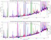 |
Fig. B.1. Unscaled (top) and scaled (bottom) full spectral scans. The spectra were extracted from the TH2 position in the low resolution data (see Sect. B). The colors in the spectra represent the spectral windows from the lower side band (red and blue) and the upper side band (green and violet). A dotted line indicates the atmospheric transmission for a PWV of 1 mm. |
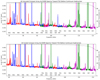 |
Fig. B.2. Same as Fig. B.1, but for Band 3 unscaled (top) and scaled (bottom). Additionally the label for each of the individual spectral setups (see Sect. 2) are displayed. |
Appendix C: ALCHEMI Flux Calibration
The ALMA flux calibration process includes a number of contributions to its uncertainty, including systematic errors within a given measurement calibrated with a single primary flux reference such as that due to:
-
The primary flux calibrator model used to set the absolute flux calibration scale.
-
The primary flux calibrator measurement used to define the reference point for the secondary flux calibrator flux.
as well as random uncertainties due to:
-
The bootstrapping from the primary to the secondary flux calibrator.
-
The bootstrapping from the secondary flux calibrator to the target source.
-
The lack of a proper elevation-dependent opacity correction during any of the bootstrapping steps.
Furthermore, even though extra mitigation measures can be done during an observation to account for items 4 and 5 above, there is nothing that can allow one to attain an absolute flux calibration error that is better than the error associated with the primary flux calibrator measurement and model.
Early in the process of imaging the ALCHEMI measurements, amplitude offsets between overlapping receiver tunings were noted (see Sect. 3.1 and Appendix B). The analysis of these offsets has given ALCHEMI the ability to correct for “at least one component” of the flux calibration uncertainty. This flux calibration alignment, though, does not allow for the determination of the absolute flux calibration reference. At best we have corrected the flux scales within our individual scheduling blocks to a common value. The ALCHEMI image cubes have been corrected for these flux rescaling factors, which we believe has corrected for noise introduced as part of the flux calibration process after the primary flux calibrator measurement.
In the following we address two levels of flux calibration uncertainty in the ALCHEMI data: Relative flux calibration, which represents the flux calibration uncertainty to be used when comparing fluxes within the ALCHEMI image cubes for a given set of imaging inputs (i.e., array, spatial, and spectral resolution); Absolute flux calibration, which represents the flux calibration uncertainty to be used when comparing fluxes derived from the ALCHEMI image cubes for comparison with other (non-ALCHEMI) measurements.
C.1. Relative Flux Calibration Uncertainty
The spectral flux normalization that we have applied to all ALCHEMI measurement sets has effectively normalized all ALCHEMI data to a common flux calibration scale for each array configuration5 measured in the ALCHEMI survey. This implies that we have normalized all ALCHEMI data measured with a given array configuration to the same relative flux calibration scale. This furthermore implies that comparison of spectral lines within the ALCHEMI survey can be compared using a relative flux calibration uncertainty.
The statistics of the amplitude scaling factors given in Table A.1 are provided in Table C.1. It is noteworthy that for our Band 3 measurements the 12mE configuration shows significant deviations from the average values of the scaling factors for that receiver band and configuration.
Statistics by bands and arrays of the relative flux scaling factors (ai)
An estimate of the relative flux calibration uncertainty associated with a given receiver band and configuration can be derived from the scatter in the scaling factors (Table C.1) that we have applied to our measurement sets to normalize them to the same mean flux scale. The RMS values for the flux scale normalization factors for each Band and array configuration(s) (listed as Compact Array / Extended Array / Combined) are:
-
Band 3: 2% / 12% / 12%
-
Band 4: 1% / 2% / 2%
-
Band 5: 2% / 2% / 2%
-
Band 6: 5% / 1% / 5%
-
Band 7: 8% / 3% / 9%
The relative flux calibration uncertainty for the ALCHEMI image cubes which are combinations of the Compact Array and Extended Array measurements will in reality be a complex combination of the relative flux calibration uncertainties, which itself depends upon the contribution of each array measurement to a given flux in the ALCHEMI survey. The contribution of each array to the combined measurement is dependent upon numerous factors such as relative visibility contributions and time-dependent variations between the individual array measurements. In the above, we conservatively estimate the relative flux calibration uncertainty for the combined values as the root-sum-square of the Compact Array and Extended Array scaling factor RMS values.
Be aware that the actual "flux uncertainty” to be used in a line-ratio analysis, for example, is not determined solely by the “flux calibration uncertainty” in complex sources such as NGC 253. The line flux one measures depends on how the imaging process (robust parameter, clean mask, clean depth, selfcal, etc.) has been performed and on the properties of the spectral line itself. The same imaging parameters can have different effects on different spectral lines. For example, when different spectral lines have distinct spatial extents or when one spectral line is bright and the other is faint because the brighter spectral line has a larger fraction of its flux cleaned. For these reasons, the real flux calibration uncertainty is likely to be larger than that assumed from an assessment of the quality of the flux calibration process alone.
C.2. Absolute Flux Calibration Uncertainty
The absolute flux calibration uncertainty starts with the relative flux calibration uncertainty and includes contributions due to the measurement, model, and application of the primary flux calibration source (see above). To estimate this additional contribution, we assume that the measurement of the relatively bright sources used as primary flux calibrators provide a negligible contribution to the primary flux calibration uncertainty. This uncertainty is then dominated by that associated with the primary flux calibrator model. Models used by ALMA within CASA are unlikely to be accurate to < 5% (Butler 2012, priv. comm.). We use then the following recommendations for flux calibration accuracy, from the ALMA Proposer’s Guide for Cycle 52 (Section A.9.2 on "Flux Accuracy"), as an estimate of the primary flux calibrator model uncertainty:
-
Bands 3, 4, 5: < 5%
-
Bands 6, 7, 8: < 10%
-
Bands 9 and 10: < 20%
The absolute flux calibration uncertainty, including the relative flux calibration uncertainty derived for the ALCHEMI image cubes, is given by the root-sum-squared of the relative and primary flux standard model calibration uncertainties (listed as in Sect. C.1):
-
Band 3: 5% / 13% / 13%
-
Band 4: 5% / 5% / 5%
-
Band 5: 5% / 5% / 5%
-
Band 6: 11% / 10% / 11%
-
Band 7: 13% / 10% / 13%
Therefore, for the sake of simplicity, we recommend the usage of a conservative 15% uncertainty for the absolute flux calibration within the ALCHEMI image cubes, at any frequency and configuration.
C.3. A Search for the ALCHEMI Flux Normalization Anomalies
We find that 11 of the 47 tunings (∼23%) which comprise the ALCHEMI data set have amplitude scale factors which are larger than the ALMA amplitude calibration specification of 5%, with the two most discrepant tunings being 26% (Band 7) and 21% (Band 3). Table C.2 lists the measurement information for the 11 discrepant tunings.
ALCHEMI tunings with discrepant amplitude calibration
In an attempt to determine the source(s) of the thirteen science goals with poor amplitude calibration, we have investigated how ALMA calibrates amplitude within the limits of the information provided to investigators. ALMA flux calibration is made within a given observation (or “execution block”) by measurement of a standard quasar selected from a list of monitored quasars, referred to as the “grid sources”. ALMA strives to measure these standard quasars at least once every 14 days at bands 3 and 7, and calibrates their fluxes to an absolute scale through reference measurements of primary flux calibrators (i.e., Uranus). The measured absolute fluxes for the grid source calibrators are available from the ALMA calibrator archive. We have extracted the flux scaling information from the calibration pipeline weblog file “flux.csv” associated with each observing execution block (EB). This flux scaling information includes the “spectral index age” and time since the standardized flux for each calibrator was derived.
C.3.1. Possible Source of Error: Large Spectral Index Age (spixAge)
As the spectral index age (spixAge) is one of the factors used by getALMAFlux to extrapolate measured flux calibrator fluxes to target frequencies, there was a concern that perhaps large spixAge factors were causing the large flux calibration errors. Using the spectral index age information extracted from the pipeline calibration process we show the correlation between spectral index age and amplitude scale factor in Figure C.1. There is no correlation between spixAge and the amount of the flux calibration error.
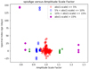 |
Fig. C.1. Correlation between spectral index age and amplitude scale factor for all ALCHEMI measurements. Coloring is used to designate ranges of amplitude scaling. |
C.3.2. Possible Source of Error: Calibrator Catalog Band 3 Age
By inspecting the age of the absolutely calibrated Band 3 flux used by getALMAFlux (extracted from the flux.csv files associated with the pipeline calibration process), we find that there is no apparent correlation between the "Age"/"Band3Age" and large amplitude scaling factors. The "Age" or "Band3Age" is in almost all cases between 0 and 3 days for our most discrepant scale factor EBs. In one case it was 6 days, and another was 5 days, but neither of these were from our "worst cases". Band 3 age does not appear to be a likely source for the discrepant amplitude scale factors.
C.3.3. Possible Source of Error: Flux Monitoring Time Gaps
Many, though not all, of the science goals (SGs) with discrepant amplitude scale factors occur just after a gap in the respective flux calibrator measurements. Specifically, for 8 of the 13 discrepant Band 3 SGs, there was a significant flux calibrator measurement time gap just before these SGs were observed, and this correlation between flux calibrator measurement time gap and discrepant scale factor does not exist for Band 6 (green) or Band 7 (black) SGs with discrepant amplitude scale factors. Although this may be an explanation for the excessive Band 3 flux calibration uncertainties, a time gap in the flux monitoring for our flux calibrators does not appear to be consistent for all SGs with discrepant flux calibration.
C.3.4. Possible Source of Error: Large Time Span Between System Temperature Measurements
By perusing the weblogs associated with the ALCHEMI measurements we know that the scaling from raw amplitude to a temperature scale (otherwise known as the “system temperature” measurement), was routinely made only every ∼11 minutes at Band 3 and every ∼8 minutes at Band 7. As these system temperature measurements are required to track the changes in sky emission as a function of time, it could be that these basic amplitude scaling factors have not been sampled well enough in time, especially at the higher frequency bands. However this is an observatory trade-off between enhanced calibration accuracy and observing efficiency.
C.3.5. Possible Source of Error: Noisy Gain Calibrator Measurement
For the SG with the most discrepant flux calibration, B7d 7m (ngc253_d_07_7M) there may be an issue with gain calibrator phase stability. Three out of five execution blocks (EBs) for the scheduling block (SB) were taken on the same day (2018-01-21). J0038−2459 was observed as the gain calibrator for all the three EBs. Although the gain calibrator flux is expected to be stable over the three EBs, because the flux is very likely to be stable over the short time scale between these three EBs (about six hours), the derived flux densities in the pipeline calibration changed about 28% (peak-to-peak). The following is a summary of the pipeline-derived flux densities of the phase calibrator (reference: the weblog, stage 15).
# EB                            start date/time (UT)
  flux density (spw 16)
uid___A002_Xc96f17_X8658        2018-01-21 19:06:14
  1024.0+-9.979 mJy
uid___A002_Xc96f17_X8ec1        2018-01-21 22:17:40
  855.121+-12.804 mJy
uid___A002_Xc96f17_X92b9        2018-01-21 23:53:08
  797.500+-5.496 mJy
It is possible that poor atmospheric phase stability is the cause of the large flux calibration uncertainty, as all the EBs were taken in the late afternoon to early evening, which is the part of the day when the atmospheric phase stability tends to be very the poorest. In fact, in the calibrated visibility amplitude vs time plot of the EB (weblog stage 17) one can see frequent amplitude drops in the Bandpass/Flux calibrator scan.
Another example of a correlation between poor phase stability and poor flux calibration is B3b 12mE (ngc253_b_03_TM1). As was the case for B7d 7m, the EBs for this SB were also affected by large phase fluctuations, and that they were also executed in daytime (late afternoon). Figure C.2 shows the pipeline plots of amplitude vs time for all the EBs for B3b 7m. Significant amplitude drops in the bandpass/amplitude calibrator (J2258−2758) can be seen especially in EB uid___A002_Xcb1740_X94c9, and they could affect the flux scaling of the gain calibrator.
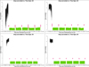 |
Fig. C.2. B3b 7m amplitude/bandpass calibrator flux versus time weblog plots for the four EBs in this SB. |
The following is a summary of the pipeline-derived flux density of gain calibrator J0038−2459 (reference: the weblog, stage 15).
spw=25
uid___A002_Xcb1740_X94c9        2018-03-27 18:36:03
 955.851+-14.748 mJy
uid___A002_Xcb339b_X600b        2018-03-29 14:10:14
 938.721+-7.809 mJy
uid___A002_Xcb339b_X633f        2018-03-29 15:30:21
 903.452+-9.069 mJy
uid___A002_Xcb339b_X68ab        2018-03-29 17:57:08
 941.212+-1.904 mJy
The change of delivered flux density looks relatively large (5.8% in peak-to-peak) even though the EBs were taken within three days. This could be an explanation for the discrepant flux calibration (second worst of all SGs) for this SG.
In order to assess the effect of a large gain calibrator flux uncertainties on the derivation of our flux calibration uncertainty for all of the ALCHEMI SGs, we have extracted all derived gain calibrator fluxes and uncertainties from the ALCHEMI weblogs. We have derived a normalized gain calibration error for each SG by doing the following: Firstly, we calculate the weighted uncertainty (σgain) for all gain calibrator measurements; Secondly, we average normalized gain calibrator uncertainties ( ) over all spectral windows and measurements taken within 5 days of each other. This time window is expected to be shorter than any changes in the absolute flux of the gain calibrator; Finally, by using a normalized gain calibrator uncertainty, we are attempting to smooth-out any changes in gain calibrator flux measurement uncertainty due to differences in gain calibrator integration time.
Figures C.3, C.4, and C.5 show examples of gain calibrator measurements, with weighted uncertainties, and their associated weighted average as a function of frequency. Figure C.6 shows the correlation between normalized gain calibrator standard deviation (as a percentage) versus the associated amplitude calibration scale factor (calculated as a difference from a perfect amplitude scale factor of 1.0). Even though in a few cases large normalized gain calibration errors are associated with large amplitude scale factors, there is no systematic correlation between these measures.
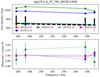 |
Fig. C.3. Sample gain calibration results for all EBs associated with B7d 7m. The bottom panel shows the residual from a linear fit for each measurement date to the measured flux densities displayed in the top panel. |
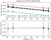 |
Fig. C.4. Sample gain calibration results for all EBs associated with B3b TM1. Same diagram style as used in Figure C.3. |
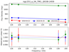 |
Fig. C.5. Sample gain calibration results for all EBs associated with B4a TM1. Same diagram style as used in Figure C.3. |
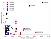 |
Fig. C.6. Correlation between normalized gain calibrator standard deviation (as a percentage) versus the associated amplitude calibration scale factor (calculated as a difference from a perfect amplitude scale factor of 1.0). Tunings with larger than 12% scale factors are annotated. See above description for calculation details. |
C.4. Conclusion to Search for ALCHEMI Flux Normalization Anomalies
In Sections C.3.1 through C.3.5 we have investigated the possible sources of the discrepant flux calibration uncertainties derived for 13 of the ALCHEMI SBs. We find that with the exception of possible errors in Tsys measurement, which we are unable to properly analyze, none of the above potential sources of error appear to explain all of our discrepant amplitude calibration.
Appendix D: Fitting details of individual species
Sect. 4.3.2 provided details on the procedure used to fit the modeled synthetic spectra to the low resolution ACA observations. In summary, the procedure consists on a human-supervised automatic fit, where the only intervention aims at ensuring convergence of the fit. Additional criteria used for the newly detected species (Sect. 4.4) are provided below in Sect. D.1. Thus, parameters were fixed or transitions were masked in the fit when convergence could not be achieved. The results are reported in Table. A.3. Here we note that in some cases, the large uncertainty in the fit to the temperature resulted in column density errors of the same order as the value fitted. Such is the case of H13CN, despite being a clear detection with bright features, extra masking and fixing of the temperature was required to provide a reasonably narrow error on the column density (with only marginal change in the fitted column density value). However in most cases we decided to maintain such fits for the sake of consistency with the procedure applied to all species.
Although we know from previous studies that there is evidence for the presence of multiple components with different excitation temperatures (Aladro et al. 2011b), there are no really obvious deviations from the LTE fit. As an example the higher energy transitions of HC3N appear to be underestimated, which could support the presence of a higher temperature component. Similarly H2CO is not that well fitted under LTE, showing flat topped spectral features. For the sake of simplicity in the presentation of these data, we assumed a single LTE component for all species. A detailed analysis of the excitation of some of these species will be presented in future publications which will make use of the higher resolution ALCHEMI 12m Array data.
For the sake of completeness, a list of all transitions above a peak flux density of 15 mJy are presented in Table D.1. We note that these intensities correspond to those of the model fit to the observed spectra, and therefore parameters of velocity and width are those corresponding to the species as presented in Table A.3. As indicated in Sect. 4.3.2, no measurement or analysis of individual spectral features has been performed. For the reasons presented there, analysis has been performed per molecular species.
Intensities from the 744 transitions with > 15 mJy from the LTE model fit to the data
Below we provide some cases of transitions significantly deviating from LTE together with other special details on the fitting of individual species.
H3O+: The fit to H3O+ emission has been performed only on the 307.2 GHz transition, which is one of the two transitions covered by our survey. Although the 307.2 GHz is blended with CH3OH, this contribution is accounted for based on the CH3OH fit to the whole survey. The 364.8 GHz transition, on the other hand, is the most obvious case of non-LTE emission, and is observed to be more than an order of magnitude brighter than predicted by LTE (Fig. F.11) The line ratio between these two transitions has been calculated based on the individual integrated intensity fit to each transition and not on the LTE intensities in Table. D.1. To explain the relatively large observed flux density ratio of S364.8/S307.2 = 6.8 ± 1.0 between the two transitions, non-LTE models from Phillips et al. (1992) suggest volume densities < 107 cm−3 and effective excitation by dust emission. Together with the vibrational emission reported in Sect. 5.2, H3O+ is also probing the importance of infrared pumping in NGC 253 GMCs. However, the 396 GHz transition of H3O+, not covered in our survey, is key to constrain the non-LTE physical conditions of the emitting gas. All other species below that show transitions not well fitted by the LTE approximations, are not as extreme as the case of H3O+ where, as mentioned above, the LTE approximation is underestimating the 364.8 GHz by more than an order of magnitude.
H2S: The transition of H2S at 216.71 GHz is approximately two times brighter than predicted by the LTE fit.
H2CO: The transitions at 140.83 and 150.48 GHz are twice as bright as predicted by the LTE fit. A number of other transitions also deviate from the fit, but to a lesser extent. We note that we did not fit the ortho- and para-H2CO separately, but we assumed the ortho-to-para ratio of 3.
HC3N: All transitions above 270 GHz are brighter than the LTE fit estimate. This could be the signature of a warmer component and partially to the effect of varying opacity across the transitions.
HNCO: The brighter transitions of HNCO show an obvious double peak profile which is likely due to the distribution of this species at high resolution (Meier et al. 2015). This double peak profile, similarly observed in CH3OH, is more apparent than in other species where the velocity components are more blended and the profile is a single peak. On the other hand, many of the fainter transitions of HNCO are overestimated by the LTE fit.
CH CCH: Despite being almost uniformly blended with other species, the fit of
  is consistent within the errors to that of the other two isotopologues, being ∼0.1 dex above
  and ∼0.4 dex above 13CH3CCH. Although the uncertainties in the column density determination of the latter two isotopologues are of the same order as the value fitted, an independent fit to the three isotopologues are in good agreement, which supports the detection and fit to those species. Moreover, the ratio to the main isotopologue (Table 4) is consistent with what is observed with other species as discussed in Sect. 5.4.1).
CH3OH: Two of the transitions of methanol, the 11, 0 − 20, 2 at 205.79 GHz and 71, 7 − 61, 6 at 335.58 GHz, show observed fluxes which are less than half of the LTE fit flux, while the 61, 5 − 51, 4 at 292.7 GHz transition is about half of the LTE fit flux. Similar to what is observed in HNCO, the brighter transitions show a very clear double peak profile.
13CH3OH: There is only one transition of 13CH3OH which is bright enough and is not blended with other species. Therefore this is the only species in which the fit value should be considered with caution and probably an upper limit. This LTE fit has been discussed in Sect. 5.4.1.
CH3CN: The J = 7 − 6 and 8 − 7 groups of transitions at 128.7 and 147.1 GHz, respectively, show significantly brighter emission than that from the LTE fit, being up to a factor of two brighter on the former.
CH2NH: While the 31, 1 − 10, 1 transition at 166.85 GHz is not detected, though predicted by the LTE fit, the 20, 2 − 10, 1 transition at 127.85 GHz is brighter than predicted.
D.1. Fitting details of newly detected species
On top of the fit criteria explained in Sect. 4.3.2 on detection of the brightest spectral features and requiring convergence of the fit, we enforced extra criteria to claim newly detected species. This is, at least one of the brightest (according to the LTE prediction) spectral features needs to be un-blended or marginally contaminated by emission from other species based on the LTE modeling to other transitions from the contaminant species. More importantly, all other blended transitions should be consistent with the residual spectra after subtraction of all other modeled species. In other words, any bright emission line predicted by the LTE model should be consistent with the observed spectra and no big outliers should be present. This may not be the case with previously reported species showing some out of equilibrium transitions reported above.
In this section we present details of the modeling of C2H5OH, HOCN and HC3HO, since most relevant details regarding the newly detected isotopologues are discussed in Sect. 5.4. Figs. D.1, D.2, and D.3 show the fit results to these species where the spectral features are ordered by the brightness of the LTE modeled emission, thus showing only the brightest spectral features of each molecule.
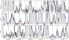 |
Fig. D.1. Modeled emission of C2H5OH in red, overlaid over the observed spectrum (filled black histogram) and the global model including all molecular transitions in this study. Only the 18 brightest transitions or group of transitions according to the LTE model of C2H5OH are displayed, ordered in descending order of brightness from left to right and top to bottom. The model generated with MADCUBA makes use of the spectroscopic parameters in JPL catalog entry 46004. The frequency of the brightest transition in each panel are displayed for reference. |
 |
Fig. D.2. Same as Fig. D.1 showing the model of HOCN, using the spectroscopic parameters in CDMS catalog entry 43510. |
 |
Fig. D.3. Same as Fig. D.1 showing the model of HC3HO, using the spectroscopic parameters in JPL catalog entry 54007. |
We do not list the spectroscopic parameters of the detected transitions since these are directly extracted from the catalog entries indicated in the figures and more importantly these species have been previously identified in the Galactic ISM.
C2H5OH: All transitions above 3 mJy modeled emission were used to fit the emission of C2H5OH, where those falling within the spectral features of significantly brighter transitions were masked, adding up to a total of ∼50 transitions considered. Among its brightest transitions only the transitions at 287.944 GHz (64, 2 − 53, 3) and 287.917 GHz (64, 3 − 53, 2) form an clearly unblended spectral feature. Other spectral lines at 252.952, 270.450, and 234.758 GHz, though partially blended, confirm the detection of C2H5OH, together with the fainter feature at 243.556 GHz also marginally blended as displayed in Fig. D.1. The identified transitions appear to show a double peak, similar to what is observed for CH3OH, further supporting this detection.
HOCN: The brightest expected transition of HOCN in the whole frequency coverage of ALCHEMIS (100, 10 − 90, 9 at 209.732 GHz) is unambiguously detected and just marginally blended. The brightness of all other transitions drop quickly below the detection limit or are blended to other brighter species as shown in Fig. D.2. All spectral features shown in this figure, but for the one at 251.666 GHz were used in the fit.
HC3HO: The two brighest transitions of HC3HO (140, 14 − 130, 13 @ 129.975 GHz and 150, 15 − 140, 14 @ 139.169 GHz) appear unblended in our survey while most other transitions fall close to the noise level of our obsrevations. We conservatively included transitions down to ∼1 mJy in the fit to this species which may have resulted in an understimate of the brightest transitions. A fit performed exclusively with the two brightest transitions would have resulted into a column density 80% higher yielding  .
.
Appendix E: Extragalactic molecular census
The continuous growth of new species detected during the last two decades has resulted in various publications reporting up to date listings of the extragalactic molecular census including conference proceedings (Martín 2009; Martín et al. 2011), refereed publications (Martín et al. 2006, 2011; McGuire 2018), as well as online resources such as that hosted at CDMS6. Each of these reports have had different formats and criteria depending on the scope of the publication but all aiming to maintain updated information on first molecular extragalactic detections. Despite these available resources, given the legacy value of ALCHEMI for the extragalactic molecular content, and the relevance of isotopologue detections in this work, which are not included in most of the references above, we provide here a detailed and updated extragalactic molecular census.
In this appendix we provide a comprehensive listing of all molecular species and isotopologues detected in the extragalactic ISM according to the chronology of detections (Table E.1) and grouped by the number of atoms in the molecule (Table E.2). Graphical representations of these lists can be found in Sect. 4.4.
Chronology of extragalactic detections.
Census of extragalactic molecular species and isotopologues detected.
Appendix F: Full spectrum and model
Fig. F.1 presents the full spectrum analyzed in this article (gray histogram) with the best LTE model fit (red line) as well as the labels for each individual transition with flux density above 100 mJy according to the LTE model. Figs. F.2 to F.11 present a zoomed version of Fig. F.1 in 5 GHz windows and labeling transitions down to 2 mJy. We note that despite what was indicated in Table A.1, the spectral window centered at 368.7 GHz could not be imaged with the 12 m data due to the poor atmospheric transmission. Despite the poorer quality of the data, this spectral window is included in Fig. F.11, which actually shows a bright spectral feature due to H2S. The quality of the data can only be used to confirm the presence of the line but was not included in the fit.
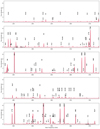 |
Fig. F.1. Full spectral coverage as in Fig.4 zoomed to 50 GHz frequency windows. The observed spectrum is shown in grey histogram and the model (Sect. 4.3.2) in red line. Only the brighter individual molecular transitions with intensities higher than 100 mJy are labeled with different y-axis position and character size depending on the modelled intensity for > 5, > 1,> 0.2, and > 0.1 Jy. |
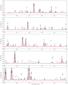 |
Fig. F.2. Full spectral coverage as in Fig.4 zoomed to 5 GHz frequency windows. The observed spectrum is shown in grey histogram and the model (Sect. 4.3.2) in red line. Individual molecular transitions with intensities higher than 2 mJy are labeled with different y-axis position and character size depending on the modelled intensity for > 270, > 95, > 40, > 20, > 15, > 10, > 5, and > 2 mJy. |
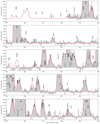 |
Fig. F.10. Same as Fig. F.2. |
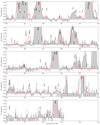 |
Fig. F.11. Same as Fig. F.2. |
All Tables
Spectral line emission properties of the vibrational transitions of HCN, HNC, and HCO+.
Intensities from the 744 transitions with > 15 mJy from the LTE model fit to the data
All Figures
|
Fig. 1. Schematic summary of the activity within central molecular zone of NGC 253. See Sect. 1 for a comprehensive summary of the activity in its central region as probed by multiwavelength observations. In both figures, the CO traced CMZ, and the dense gas traced GMCs (Leroy et al. 2015) are included as a spatial scale reference. Left: IRAC 8μm from Spitzer Local Volume Legacy survey (Dale et al. 2009) in the background; Chandra X-ray traced outflow (Strickland et al. 2000); 18 cm OH plume (Turner 1985); molecular outflow observed in CO emission (Bolatto et al. 2013). Right: 2 cm TH sources (Turner & Ho 1985) and HII regions and supernovae remnants (Ulvestad & Antonucci 1997); proto-super stellar clusters traced by vibrationally excited HC3N emission (Rico-Villas et al. 2020); star cluster identified from near-IR HST imaging (Watson et al. 1996). |
| In the text | |
|
Fig. 2. Measured RMS flux density (top) and equivalent brightness temperature (bottom) noise level of each individual data cube (spectral windows) imaged for the combined arrays (blue), compact 12 m array band 3 observations (green) and 7 m array band 4 to 7 (red). Black lines correspond to the target sensitivities requested for 1″ (top) and |
| In the text | |
|
Fig. 3. Maximum recoverable scale per channel estimated for each individual 12-m (red) and 7-m (blue) array observations (Sect. 2.3). Each point corresponds to an individual execution centered at the average frequency of all four spectral windows (thus the gaps that appear in some frequencies). The targeted 15″ maximum recovered scale is represented by an horizontal black line. |
| In the text | |
|
Fig. 4. Full spectral coverage obtained with the ALMA Compact Array (ACA 7m) alone, extracted from the position of brightest molecular emission (see Sect. 4.3.1). Figure F.1 presents a zoomed version of this plot in five frequency windows 50 GHz wide where the comparison with the modeled emission (Sect. 4.3.2) and the molecular line identification of each individual feature is included. Figures F.2–F.11 present a further zoomed version in 5 GHz windows. |
| In the text | |
|
Fig. 5. Continuum flux density at the peak of emission as derived from each spectral window across the surveyed frequency range (red dots). We note that extended emission in our data might account for up to ∼20% higher fluxes (Sect. 4.1). A fit to the data is shown by a continuous blue line, which is the combination of the free-free emission (dotted blue almost horizontal line) and the graybody emission (dashed blue line). See text for further details on parameters used. As a reference to illustrate the deviation from pure black body emission, that for a Td = 50 K and 0.5″ source size is shown as a green dot-dashed line. |
| In the text | |
|
Fig. 6. Spectral line contribution to the continuum flux in 5 GHz bins. The position of spectral features brighter than 1 Jy are shown as blue segments at their corresponding frequency, with the two CO J = 2 − 1 and 3 − 2 transitions displayed in yellow. |
| In the text | |
|
Fig. 7. Sample of integrated flux density moment 0 maps from 16 of the brightest molecular transitions in the covered frequency band. Each panel is labeled with the corresponding molecular species and transition. We point out that CO 1 − 0 is not included since Band 3 is not covered by the ACA data. In color the combined 12 m+7 m maps are shown where the color coding is adjusted for visibility of each individual species. Gray contours show the 7 m integrated intensity images where the n-th contour level corresponds to 20 n3 Jy km s−1 beam−1 for all species. Species are ordered in decreasing order of integrated flux density from left to right and from top to bottom. The panel in the lower left shows the reference coordinates and the beam size of the combined 12 m+7 m ( |
| In the text | |
|
Fig. 8. Top: histogram showing the number of spectral lines above 2 mJy in the model in bins of flux density. Lines between 2 mJy and 10 Jy are considered. The three spectral features with flux densities above 10 Jy are not included in this diagram. Bottom: histogram showing the number of spectral lines above 2 mJy in frequency bins of ∼5 GHz width. |
| In the text | |
|
Fig. 9. Chronology of extragalactic molecular detections including those reported in this work. Detections of main and rarer isotopologue substitutions in blue and gray respectively, with the total number of detections, not considering tentative reports, being displayed in dark blue. One and two year bins are used for top and bottom panel histograms, respectively. |
| In the text | |
|
Fig. 10. Number of individual detectable species as a function of the flux density level relative to the brighter transitions detected in the survey per band. Left: flux density levels are referred to the CO 3 − 2 (112 Jy beam−1) as the brightest transition detected in the whole spectral range covered. Right: flux densities are referred to the brightest transition detected on each band. This is CS 3 − 2 (0.9 Jy beam−1 in Band 4), HCO+ 2 − 1 (3 Jy beam−1 in Band 5), CO 2 − 1 (56 Jy beam−1 in Band 6), and CO 3 − 2 (in Band 7). |
| In the text | |
|
Fig. 11. Rotational transitions in the vibrational state v2 = 1f of HCN, HNC and HCO+ covered within the surveyed frequency range. The box corresponding to HNC 2 − 1 v2 = 1f was left intentionally blank since its emission at 182.6 GHz falls within the telluric water transition observation gap (Sect. 2). Red lines show an attempt to fit the observed emission under LTE assuming Tex = 300 K (see text in Sect. 5.2 for details). Nearby transitions from detected species with modeled flux densities > 10% of that of the vibrational transitions are labeled. |
| In the text | |
|
Fig. 12. Abundances of C2H5OH and HCOOH relative to CH3OH toward the NGC 253 CMZ (orange star), compared to those measured toward Galactic hot cores (red squares; Ikeda et al. 2001) and Galactic Center giant molecular clouds (green circles; Requena-Torres et al. 2006). Upper limits to C2H5OH and HCOOH are represented by open symbols. |
| In the text | |
|
Fig. 13. Measured NGC 253 isotope ratios in the ACA data (Table 4) compared to their equivalent values in the Milky Way (Wilson 1999). The horizontal axis indicates the molecular species, or in the case of CO the isotopomer, used to measure a given isotope ratio. Colored rectangles are used to indicate Milky Way isotope ratio value ranges. As no uncertainties nor range of values was provided for the Si isotope ratios, a range of 10% of the estimated values was assumed. As the Milky Way 16O/17O value would be ≳875, we have opted to not show this Milky Way isotope ratio value. |
| In the text | |
|
Fig. 14. Spectral features of the J = 4 − 3 (left), 3 − 2 (center) and 2 − 1 (right) transitions from three of the isotopologues of CCH detected in the survey. Red curves shows the LTE model best fits. Contributions by other species is almost negligible for most transitions according to the global LTE model from the full survey (see Sect. 4.3.2). However we note that the observed profile of 13CCH 4−3, not following the CCH LTE model and not accounted for by emission from other species, was not used in the fit. |
| In the text | |
|
Fig. 15. Spectral features of the J = 3 − 2 (left) and 2 − 1 (right) transitions from three of the rarer isotopologues of carbon monoxide detected in the survey. Red curves show the LTE model best fits. Contributions by other species are not shown since all features appear to be free of contamination. |
| In the text | |
|
Fig. 16. CN N = 3 − 2 (top) and N = 2 − 1 (bottom) emission measured with the ACA data presented in this article. Panels are centered at 340.248 and 226.874 GHz, which is the frequency of the stronger emission hyperfine transition. The data are fitted with three simple models. Left: single component corresponding to the fit presented in Sect. 4.3.2, where a source size θs = 5″ is assumed. The central opacity of the brightest transitions are τ3 − 2 = 0.25 and τ2 − 1 = 0.44, while the cumulative opacity of the stronger hyperfine groups are |
| In the text | |
|
Fig. B.1. Unscaled (top) and scaled (bottom) full spectral scans. The spectra were extracted from the TH2 position in the low resolution data (see Sect. B). The colors in the spectra represent the spectral windows from the lower side band (red and blue) and the upper side band (green and violet). A dotted line indicates the atmospheric transmission for a PWV of 1 mm. |
| In the text | |
|
Fig. B.2. Same as Fig. B.1, but for Band 3 unscaled (top) and scaled (bottom). Additionally the label for each of the individual spectral setups (see Sect. 2) are displayed. |
| In the text | |
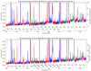 |
Fig. B.3. Same as Fig. B.2 but for Band 4 unscaled (top) and scaled (bottom). |
| In the text | |
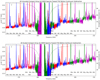 |
Fig. B.4. Same as Fig. B.2 but for Band 5 unscaled (top) and scaled (bottom). |
| In the text | |
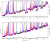 |
Fig. B.5. Same as Fig. B.2 but for Band 6 unscaled (top) and scaled (bottom). |
| In the text | |
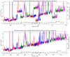 |
Fig. B.6. Same as Fig. B.2 but for the first-half of Band 7 unscaled (top) and scaled (bottom). |
| In the text | |
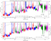 |
Fig. B.7. Same as Fig. B.2 but for the second half of Band 7 unscaled (top) and scaled (bottom). |
| In the text | |
|
Fig. C.1. Correlation between spectral index age and amplitude scale factor for all ALCHEMI measurements. Coloring is used to designate ranges of amplitude scaling. |
| In the text | |
|
Fig. C.2. B3b 7m amplitude/bandpass calibrator flux versus time weblog plots for the four EBs in this SB. |
| In the text | |
|
Fig. C.3. Sample gain calibration results for all EBs associated with B7d 7m. The bottom panel shows the residual from a linear fit for each measurement date to the measured flux densities displayed in the top panel. |
| In the text | |
|
Fig. C.4. Sample gain calibration results for all EBs associated with B3b TM1. Same diagram style as used in Figure C.3. |
| In the text | |
|
Fig. C.5. Sample gain calibration results for all EBs associated with B4a TM1. Same diagram style as used in Figure C.3. |
| In the text | |
|
Fig. C.6. Correlation between normalized gain calibrator standard deviation (as a percentage) versus the associated amplitude calibration scale factor (calculated as a difference from a perfect amplitude scale factor of 1.0). Tunings with larger than 12% scale factors are annotated. See above description for calculation details. |
| In the text | |
|
Fig. D.1. Modeled emission of C2H5OH in red, overlaid over the observed spectrum (filled black histogram) and the global model including all molecular transitions in this study. Only the 18 brightest transitions or group of transitions according to the LTE model of C2H5OH are displayed, ordered in descending order of brightness from left to right and top to bottom. The model generated with MADCUBA makes use of the spectroscopic parameters in JPL catalog entry 46004. The frequency of the brightest transition in each panel are displayed for reference. |
| In the text | |
|
Fig. D.2. Same as Fig. D.1 showing the model of HOCN, using the spectroscopic parameters in CDMS catalog entry 43510. |
| In the text | |
|
Fig. D.3. Same as Fig. D.1 showing the model of HC3HO, using the spectroscopic parameters in JPL catalog entry 54007. |
| In the text | |
|
Fig. F.1. Full spectral coverage as in Fig.4 zoomed to 50 GHz frequency windows. The observed spectrum is shown in grey histogram and the model (Sect. 4.3.2) in red line. Only the brighter individual molecular transitions with intensities higher than 100 mJy are labeled with different y-axis position and character size depending on the modelled intensity for > 5, > 1,> 0.2, and > 0.1 Jy. |
| In the text | |
|
Fig. F.2. Full spectral coverage as in Fig.4 zoomed to 5 GHz frequency windows. The observed spectrum is shown in grey histogram and the model (Sect. 4.3.2) in red line. Individual molecular transitions with intensities higher than 2 mJy are labeled with different y-axis position and character size depending on the modelled intensity for > 270, > 95, > 40, > 20, > 15, > 10, > 5, and > 2 mJy. |
| In the text | |
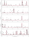 |
Fig. F.3. Same as Fig. F.2. |
| In the text | |
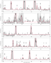 |
Fig. F.4. Same as Fig. F.2. |
| In the text | |
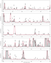 |
Fig. F.5. Same as Fig. F.2. |
| In the text | |
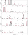 |
Fig. F.6. Same as Fig. F.2. |
| In the text | |
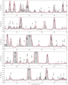 |
Fig. F.7. Same as Fig. F.2. |
| In the text | |
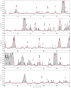 |
Fig. F.8. Same as Fig. F.2. |
| In the text | |
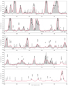 |
Fig. F.9. Same as Fig. F.2. |
| In the text | |
|
Fig. F.10. Same as Fig. F.2. |
| In the text | |
|
Fig. F.11. Same as Fig. F.2. |
| In the text | |
Current usage metrics show cumulative count of Article Views (full-text article views including HTML views, PDF and ePub downloads, according to the available data) and Abstracts Views on Vision4Press platform.
Data correspond to usage on the plateform after 2015. The current usage metrics is available 48-96 hours after online publication and is updated daily on week days.
Initial download of the metrics may take a while.