| Issue |
A&A
Volume 675, July 2023
|
|
|---|---|---|
| Article Number | A151 | |
| Number of page(s) | 32 | |
| Section | Extragalactic astronomy | |
| DOI | https://doi.org/10.1051/0004-6361/202245659 | |
| Published online | 14 July 2023 | |
Reconstructing the shock history in the CMZ of NGC 253 with ALCHEMI
1
Leiden Observatory, Leiden University, PO Box 9513, 2300 RA Leiden, The Netherlands
e-mail: This email address is being protected from spambots. You need JavaScript enabled to view it.
2
Department of Physics and Astronomy, University College London, Gower Street, London WC1E6BT, UK
3
National Radio Astronomy Observatory, 520 Edgemont Road, Charlottesville, VA 22903-2475, USA
4
European Southern Observatory, Alonso de Córdova, 3107, Vitacura, Santiago 763-0355, Chile
5
Joint ALMA Observatory, Alonso de Córdova, 3107, Vitacura, Santiago 763-0355, Chile
6
National Astronomical Observatory of Japan, 2-21-1 Osawa, Mitaka, Tokyo 181-8588, Japan
7
Institute of Astronomy and Astrophysics, Academia Sinica, 11F of AS/NTU Astronomy-Mathematics Building, No. 1, Sec. 4, Roosevelt Rd, Taipei 10617, Taiwan
8
Department of Astronomy, School of Science, The Graduate University for Advanced Studies (SOKENDAI), 2-21-1 Osawa, Mitaka, Tokyo 181-1855, Japan
9
Department of Space, Earth and Environment, Chalmers University of Technology, Onsala Space Observatory, 43992 Onsala, Sweden
10
Department of Physics, Faculty of Science and Technology, Keio University, 3-14-1 Hiyoshi, Yokohama, Kanagawa 223–8522, Japan
11
Institute of Astronomy, Graduate School of Science, The University of Tokyo, 2-21-1 Osawa, Mitaka, Tokyo 181-0015, Japan
12
Institute of Space Sciences (ICE, CSIC), Campus UAB, Carrer de Magrans, 08193 Barcelona, Spain
13
New Mexico Institute of Mining and Technology, 801 Leroy Place, Socorro, NM 87801, USA
14
National Radio Astronomy Observatory, PO Box O, 1003 Lopezville Road, Socorro, NM 87801, USA
15
Department of Astronomy, University of Virginia, PO Box 400325, 530 McCormick Road, Charlottesville, VA 22904-4325, USA
16
Max-Planck-Institut für Radioastronomie, Auf-dem-Hügel 69, 53121 Bonn, Germany
17
Astron. Dept., Faculty of Science, King Abdulaziz University, PO Box 80203, Jeddah 21589, Saudi Arabia
18
Xinjiang Astronomical Observatory, Chinese Academy of Sciences, 830011 Urumqi, PR China
19
Observatorio Astronómico Nacional (OAN-IGN)-Observatorio de Madrid, Alfonso XII, 3, 28014 Madrid, Spain
20
Centro de Astrobiología (CSIC-INTA), Ctra. de Torrejón a Ajalvir km 4, 28850 Torrejón de Ardoz, Madrid, Spain
Received:
9
December
2022
Accepted:
20
March
2023
Abstract
Context. HNCO and SiO are well-known shock tracers and have been observed in nearby galaxies, including the nearby (D = 3.5 Mpc) starburst galaxy NGC 253. The simultaneous detection of these two species in regions where the star-formation rate is high may be used to study the shock history of the gas.
Aims. We perform a multi-line molecular study of NGC 253 using the shock tracers SiO and HNCO and aim to characterize its gas properties. We also explore the possibility of reconstructing the shock history in the central molecular zone (CMZ) of the galaxy.
Methods. Six SiO transitions and eleven HNCO transitions were imaged at high resolution 1.″6 (28 pc) with the Atacama Large Millimeter/submillimeter Array (ALMA) as part of the ALCHEMI Large Programme. Both non local thermaldynamic equilibrium (non-LTE) radiative transfer analysis and chemical modeling were performed in order to characterize the gas properties and investigate the chemical origin of the emission.
Results. The nonLTE radiative transfer analysis coupled with Bayesian inference shows clear evidence that the gas traced by SiO has different densities and temperatures than that traced by HNCO, with an indication that shocks are needed to produce both species. Chemical modeling further confirms such a scenario and suggests that fast and slow shocks are responsible for SiO and HNCO production, respectively, in most GMCs. We are also able to infer the physical characteristics of the shocks traced by SiO and HNCO for each GMC.
Conclusions. Radiative transfer and chemical analysis of the SiO and HNCO in the CMZ of NGC 253 reveal a complex picture whereby most of the GMCs are subjected to shocks. We speculate on the possible shock scenarios responsible for the observed emission and provide potential history and timescales for each shock scenario. Observations of higher spatial resolution for these two species are required in order to quantitatively differentiate between the possible scenarios.
Key words: galaxies: ISM / galaxies: individual: NGC253 / astrochemistry / galaxies: starburst / ISM: molecules
Note to the reader: For a few molecules and transitions, the subscript numbers were inadvertently changed to superscript. Following the publication of the corrigendum, they were corrected on 12th October 2023.
Jansky Fellow of the National Radio Astronomy Observatory.
© The Authors 2023
 Open Access article, published by EDP Sciences, under the terms of the Creative Commons Attribution License (https://creativecommons.org/licenses/by/4.0), which permits unrestricted use, distribution, and reproduction in any medium, provided the original work is properly cited.
This article is published in open access under the Subscribe to Open model. This email address is being protected from spambots. You need JavaScript enabled to view it. to support open access publication.
1. Introduction
Many key physical and chemical processes in the interstellar medium (ISM) influence the evolution of galaxies. These processes are often associated with star formation, active galactic nuclei (AGN), large-scale outflows, and shocks. In this context, starburst galaxies are prime laboratories for the investigation of these feedback mechanisms and their impact on the ISM. As for probing these physical and chemical processes in external galaxies, multi-line multi-species molecular observations are an ideal tool, given the wide range of critical densities associated with different molecular transitions, and the dependencies of chemical reactions on the energy budget of the ISM. Past observations have suggested several useful molecules for tracing specific regions within a galaxy, such as HCO and HOC+, which are associated with the photon-dominated regions (PDRs; e.g., Savage & Ziurys 2004; García-Burillo et al. 2002; Gerin et al. 2009; Martín et al. 2009b), and HCN and CS with dense gas (e.g., Gao & Solomon 2004; Bayet et al. 2008; Aladro et al. 2011). In reality, especially in the extragalactic context where the beam size often encompasses at least several parsecs, it is seldom the case that a single gas component can be identified by observations of just one or two molecular species (Kauffmann et al. 2017; Pety et al. 2017; Viti 2017; Tafalla et al. 2021). This is because the same species can often be found in diverse environments, and multiple transitions of the same species do not necessarily come from the same gas component. As a result, molecular tracers that are uniquely sensitive to certain environments are considered extremely valuable in characterizing the physical and chemical conditions of the gas.
As starburst activities inject a significant amount of energy into the ambient environment, starburst galaxies are particularly important targets for studying the feedback mechanisms in the interstellar medium (ISM). Induced by high star-forming rates (SFRs), strong stellar feedback can trigger outflows of ionized, neutral, and molecular gas. NGC 253 is a barred spiral galaxy that is almost edge-on with an inclination of 76° (McCormick et al. 2013). Being one of the nearest starburst systems (D ∼ 3.5 ± 0.2 Mpc, Rekola et al. 2005), NGC 253 is also one of the most studied starburst galaxies. The central molecular zone (CMZ) of NGC 253 spans about 300 × 100 pc across (Sakamoto et al. 2011), and contains more than ten well-studied giant molecular clouds (GMCs); it has been observed in the continuum as well as in molecular emissions (e.g., Sakamoto et al. 2011; Leroy et al. 2015, 2018; Levy et al. 2022). NGC 253 is a prototype of nuclear starburst with an SFR of ∼2 M⊙ yr−1 coming from its CMZ (Leroy et al. 2015; Bendo et al. 2015), which is half of its global star formation activity.
A large-scale outflow in NGC 253 has been revealed by multiwavelength observations: in X-rays (Strickland et al. 2000, 2002), Hα (Westmoquette et al. 2011), molecular emission (Turner 1985; Bolatto et al. 2013; Walter et al. 2017; Krieger et al. 2019), and dust (Levy et al. 2022). This large-scale outflow is thought to be driven by the galaxy’s starburst activity (McCarthy et al. 1987), for there are no signs of AGN influence (Müller-Sánchez et al. 2010; Lehmer et al. 2013) despite there being a bright radio source associated with the nucleus of the galaxy (Turner & Ho 1985). Aside from coherent large-scale outflows, the presence of shocks and turbulence are also complementary sources of mechanical energy in the ISM feedback processes. The signature of shocks in NGC 253 has been suggested by the detection of HNCO and SiO (García-Burillo et al. 2000; Meier et al. 2015), the detection of Class I methanol masers (Humire et al. 2022), and the enhanced fractional abundances of CO2 (Harada et al. 2022).
Both silicon monoxide, SiO, and isocyanic acid, HNCO, are well-known shock tracers (Martín-Pintado et al. 1997; Hüttemeister et al. 1998; Zinchenko et al. 2000; Jiménez-Serra et al. 2008; Martín et al. 2008; Rodríguez-Fernández et al. 2010), and both have been observed in nearby galaxies (e.g., García-Burillo et al. 2000, 2010; Meier & Turner 2005, 2012; Usero et al. 2006; Martín et al. 2009a, 2015; Meier et al. 2015; Kelly et al. 2017; Huang et al. 2022) as well as Galactic sources such as star-forming regions (e.g., Mendoza et al. 2014; Podio et al. 2017; Hernández-Gómez et al. 2019; Gorai et al. 2020; Nazari et al. 2021; Canelo et al. 2021; Colzi et al. 2021), evolved stars (e.g., Velilla Prieto et al. 2015, 2017; Rizzo et al. 2021), and quiescent GMCs in the Galactic center (Zeng et al. 2018). The formation of HNCO has been suggested to take place mainly on the icy mantles of dust grains (Fedoseev et al. 2015), or possibly in the gas phase with subsequent freeze-out onto the dust grains when the temperatures are low (López-Sepulcre et al. 2015). Regardless of how it forms, ice-mantle sputtering associated with low-velocity (vs ≤ 20 km s−1) shocks can lead to an enhanced abundance of HNCO in the gas phase. The observations of HNCO toward a sample of Galactic center sources (Martín et al. 2008) have revealed a high contrast observed in its abundance between regions under the influence of shocks and intense radiation fields, showing its potential as a shock tracer. This high contrast was also shown in a sample of galaxies (Martín et al. 2009a) despite the low-resolution single-dish observations used. In fact, Kelly et al. (2017) show that HNCO can also be thermally desorbed from the surface of dust grains when the gas and dust remain coupled at higher gas densities (nH2 ≥ 104 cm−3). Therefore, HNCO may not be a unique tracer of shock activity. On the other hand, a high abundance of silicon in the gas phase can only be explained by significant sputtering from the core of the dust grains by high-velocity (vs ≥ 50 km s−1) shocks (Kelly et al. 2017). Once silicon is in the gas phase, it is expected to quickly react with molecular oxygen or a hydroxyl radical to form SiO (Schilke & Walmsley 1997). An enhanced gas-phase SiO abundance could therefore be a sensitive indicator of the heavily shocked regions.
Potentially, the simultaneous detection of HNCO and SiO in a gas where shocks are believed to take place could provide us with a comprehensive picture of its shock history. Indeed, these two species have already been proposed for the characterization of different types of shocks (fast versus slow) in the AGN-hosting galaxies, such as NGC 1068 (Kelly et al. 2017; Huang et al. 2022) and NGC 1097 (Martín et al. 2015); in the nearby weakly barred spiral galaxy IC 342, which hosts moderate starburst activity (Meier & Turner 2005; Usero et al. 2006); and in the nearby starburst galaxy NGC 253 (Meier et al. 2015). For example, in NGC 253, which is the subject of this work, HNCO 40, 4–30, 3 was found to be distinctively prominent in the outer CMZ with the HNCO(40, 4–30, 3)/SiO(2–1) intensity ratio dropping dramatically toward the inner disk, which suggests a decrease in shock strength as well as a dissipation of any shock signature by HNCO in the presence of strong radiation fields (Meier et al. 2015).
In this work, we present ALMA multitransition observations of both HNCO and SiO toward NGC 253 observed as part of the ALMA large program, “ALMA Comprehensive High-resolution Extragalactic Molecular Inventory” (ALCHEMI, Martín et al. 2021). ALCHEMI covers wide and thorough spectral scans of the CMZ of NGC 253 in the frequency range of 84.2–373.2 GHz, and provides a comprehensive molecular view towards the CMZ of NGC 253, allowing a systematic study of both the physical and chemical properties of this nearby galaxy. In the broader sense, ALCHEMI provides a uniform molecular template for an extragalactic starburst environment where systematic uncertainties are minimized, and enables a direct comparison of the ISM properties with the active star-forming environments within the Milky Way CMZ (Martín et al. 2021). The great wealth of ALCHEMI data has so far unveiled many important properties of NGC 253, including its high cosmic-ray ionization rate (CRIR; Holdship et al. 2021, 2022; Harada et al. 2021; Behrens et al. 2022). ALCHEMI has also led to the first detection of a phosphorus-bearing molecule in extragalactic sources (Haasler et al. 2022), the identification of new methanol maser transitions (Humire et al. 2022), and the use of HOCO+ as a tracer of the chemistry of CO2 (Harada et al. 2022).
This work is structured as follows. In Sect. 2, we describe the detection of multiple transitions of HNCO and SiO in the ALCHEMI data set. In Sect. 3, we present the molecular-line-intensity maps, and the spectral-line energy distribution (SLED) of HNCO and SiO, which are populated by the measured velocity-integrated line intensity from all the available excitation levels. In Sect. 4, we describe the performed nonlocal thermodynamic equilibrium (nonLTE) radiative transfer analysis and chemical modeling in order to constrain the physical conditions of the gas and the chemical origin of the emission. In Sect. 5, we further explore the comparison and physical interpretation of our results, combining both radiative transfer modeling and chemical modeling results, and discuss the potential origins of the shocks. We summarize our findings in Sect. 6.
2. Observation and data
2.1. ALCHEMI data
We briefly summarize the observational setup used to acquire the ALCHEMI survey data. Full details regarding the data acquisition, calibration, and imaging are provided by Martín et al. (2021). The ALMA Large Program ALCHEMI (project code 2017.1.00161.L and 2018.1.00162.S) imaged the CMZ within NGC 253 in the ALMA frequency Bands 3, 4, 5, 6, and 7. The rest-frequency coverage of ALCHEMI ranged from 84.2 to 373.2 GHz. The nominal phase center of the observations is α(ICRS) = 00h47m33s.26, δ(ICRS) = −25°17′17″.7. A common rectangular area with a size of 50″ × 20″ (850 × 340 pc) at a position angle of 65° was imaged to cover the central nuclear region in NGC 253. The final angular and spectral resolution of the image cubes generated from these measurements were  (∼28 pc Martín et al. 2021) and ∼10 km s−1, respectively. A common maximum recoverable angular scale of 15″ was achieved after combining the 12 m Array and Atacama Compact Array (ACA) measurements at all frequencies.
From the ALCHEMI data, we extracted the  (28 pc) resolution cubes of the CMZ of NGC 253 for the 11 HNCO transitions and 6 SiO transitions listed in Table 1. In this work we only analyze the main isotopologue species for both molecules. Also note that we only studied the Ka = 0 transitions of HNCO although in the ALCHEMI data sets some Ka ≠ 0 transitions are also detected. This choice is made so that we focus on the most robust detections, with the best signal-to-noise ratio (S/N) across the CMZ. Ka = 0 components are generally well above the 10σ level in the detected emission, while for Ka = 1 components, out of the ten regions surveyed, only two GMCs are detected at ≲3 ∼ 5 − σ. The higher energy Ka ≥ 2 components are significantly weaker. For the sake of consistency, we analyze only the Ka = 0 components for all the GMC regions. For SiO, only the vibrational ground states (v = 0) were considered. Table 1 lists relevant spectroscopic information for all HNCO and SiO transitions studied in this article. The continuum subtraction and imaging processes performed for the data used in this paper are described in Martín et al. (2021). The representative spectra of all HNCO and SiO transitions used in the current work are shown in Appendix A.
HNCO and SiO transitions used in this work.
2.2. Extraction of spectral-line emission
In order to extract integrated spectral-line intensities from our data cubes, we use CubeLineMoment1 (Mangum et al. 2019), which employs a set of spectral and spatial masks to extract integrated intensities for a defined list of target spectral frequencies. As noted by Mangum et al. (2019), the CubeLineMoment masking process uses a brighter spectral line –whose velocity structure over the galaxy is most representative of our science target lines (HNCO and SiO) in the same spectral cube– as a velocity tracer of the inspected gas component. Final products from the CubeLineMoment analysis include moment 0 (integrated intensity; Jy km s−1), 1 (average velocity; km s−1), and 2 (velocity dispersion; km s−1) images masked below a 3σ threshold (channel-based).
We selected 12 GMC regions with an aperture size equal to the ALCHEMI beam size. These regions, listed as follows, were then subjected to a quantitative analysis, which is described from Sect. 3 onward: GMC 1a, 1b, 2a, 2b, 3, 4, 5, 6, 7, 8a, 9a, and 10. The choice of these regions is based on the regions identified by Leroy et al. (2015) using dense gas tracers, and details are also discussed further by Behrens et al. (2022). In particular, the line intensity peaks in some of the GMCs on our line intensity maps are often shown to be offset from the nominal GMC positions identified by Leroy et al. (2015) in the outskirts of the CMZ. From our HNCO and SiO maps, we adopt the closest peaks to the GMC positions provided by Leroy et al. (2015) for the data with the optimal S/N. These newly designated locations are GMC 1a, 1b, 2a, 2b, 8a, and 9a. The 12 selected GMC locations are listed in Table 2 and marked in white solid circles on the maps shown in Figs. 1 and 2.
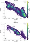 |
Fig. 1. Velocity-integrated line intensities in [K km s−1] of the HNCO transitions: (40, 4–30, 3) and (100, 10–90, 9), in (a) and (b), respectively. These two transitions are representative of the drastic variation in the trend of brightness from outer to inner GMCs. The rest of the HNCO line intensity maps are provided in Appendix B. The studied GMC regions as listed in Table 2 are labeled in white text on the map. The ALCHEMI |

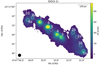 |
Fig. 2. Velocity-integrated line intensities of the SiO (2–1) transition in [K km s−1]. The remaining SiO line-intensity maps are provided in Appendix B. The studied GMC regions as listed in Table 2 are labeled in white text on the map. The ALCHEMI |

For the selected transitions used in this work, our line-intensity extraction with CubeLineMoment also includes assessment for potential contamination from neighboring lines. Following the procedure described by Holdship et al. (2021), only two lines were found with line contamination beyond the flux uncertainties: HNCO 120,12–110,11 with 34% contamination from HC3N 29–28 v = 0 (263.79230800 GHz), and SiO 7–6 with 35% contamination from OCS 25–24 v = 0 (303.99326170 GHz). The correction concerning these line contaminations was applied to the measured line intensities before further analysis was performed.
3. Velocity-integrated line intensities
In Figs. 1 and 2, we present the velocity-integrated line-intensity maps from HNCO (40, 4–30,3), HNCO (100,10–90,9), and SiO 2–1 transitions. The remaining intensity maps from other observed transitions of the two species studied in the current work are presented in Figs. B.1–B.3. For each transition map, we also overlaid all the 12 GMC regions listed in Table 2, and the ALCHEMI beam size in the lower left corner in each map. The line intensities have been converted from [Jy beam−1 km s−1] to [K km s−1]; the conversion factors are listed in Table 1.
3.1. Spatial distribution of the line emission
Looking at the spatial distribution of the line emission, the brightest emission often occurs in the inner CMZ (e.g., GMC 3/6/7) for most transitions of SiO and HNCO, except for HNCO 40,4–30,3 where GMC 1a in the outermost CMZ is the brightest region as shown in Fig. 1a. Meier et al. (2015) found HNCO 40,4–30,3 to be distinctively prominent in the outer CMZ, which is consistent with what we find here. On the other hand, these authors also found that the HNCO(40,4–30,3)/SiO(2–1) ratio drops toward the inner CMZ. Meier et al. (2015) suggested that this could be due to the decreasing shock strength and the erased shock chemistry of HNCO in the presence of a dominating central radiation field, or due to the different dependencies on temperature in the partition function of each species, because SiO is a linear molecule and HNCO is an asymmetric top (Meier et al. 2015). We want to highlight that such trends in the HNCO/SiO intensity ratio do not apply to the higher-J transition pairs, as we have already seen that the higher-J HNCO transitions are brighter in the inner CMZ (see also the comparison in Fig. 1), as are all the SiO transitions. Such complexity cannot be captured by single-transition observations, which demonstrates the importance of the multi-line observations and analysis we perform here. The trend of the intensity ratio of these two species from our data is briefly discussed in Sect. 3.2.
Within each GMC region, we further extract the beam-averaged line intensities across all available J transitions, and build up the so-called spectral-line energy distribution (SLED) by populating the same diagram with the line intensities ordered according to transition upper-level energy, Eu [K]. Figures 3 and 4 show the HNCO and SiO SLEDs, respectively. In both sets of SLEDs, we group all the collected results by color to highlight the similarities and differences in shape (the “magnitude” of the ladder, and where the ladder peaks in terms of Eu) among the GMCs. In particular, it is clear that the excitation conditions for HNCO vary substantially from one GMC to another. Globally, there is a distinction between the inner (GMC 3, 4, 5, 6, 7, represented with colored SLEDs in Fig. 3) and the outer (SLEDs in black in Fig. 3) regions of the CMZ. In the inner CMZ, we also find variation in the shapes of the molecular ladders, suggesting that interesting physics and chemistry are taking place. This variance among the subset of GMCs in the inner CMZ can be grouped as follows: GMC3 and GMC6 (in cyan), GMC4 and GMC5 (in green), and GMC7 (in orange). The first two groups –GMC3,6 and GMC4,5– have the brightest emission at mid-J excitation, between J = 7–6 and J = 12–11, across all HNCO transitions. Nevertheless, the GMC3,6 group has greater overall line intensities than GMC4/5. GMC7 tends to peak at lower Eu, suggesting that HNCO may be tracing colder gas in the inner CMZ. The SiO SLEDs (Fig. 4) have very similar shapes across all the GMCs, as also seen in the intensity maps over different J levels.
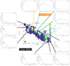 |
Fig. 3. SLED over all available energy levels of HNCO. The units are in [K km s−1]. The GMCs are categorized by the “shape” of the ladders and are labeled accordingly in different colors as described in Sect. 3: GMC3/6 (in cyan), GMC4/5 (in green), and GMC7 (in orange), and the outer GMCs: GMC 1a, 1b, 2a, 2b, 8a, 9a, and 10 (in black). The “shadowed” markers in each diagram represent nondetected points, and are displayed with an upper limit only. |
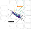 |
Fig. 4. As in Fig. 3, but for SiO. |
We note that neither HNCO nor SiO traces GMC5 particularly well in most of the transitions. Also, absorption features –due to the fact that line emission is observed against the strong continuum toward the center of the galaxy and self-absorption in the potentially optically thick regime in GMC5– have been reported from multiple ALCHEMI studies with different species (Meier et al. 2015; Humire et al. 2022). Such features are also seen in our data for GMC5. To interpret the values extracted from this region requires extra caution and a proper radiative-transfer modeling involving strong continuum emission in the background, which is beyond the scope of the present study. Additionally, in GMC10, there is a lack of detection in most transitions as shown in gray points in the SLEDs in Figs. 3 and 4. As a result, we do not discuss these two regions (GMC 5, 10) any further.
3.2. Line-intensity ratios
Variations in specific molecular line ratios are often used as probes of the physical characteristics and energetic processes in galaxies (see detailed discussion by Krips et al. 2008). This method relies on the assumption that the ratio of spectral-line intensities may be proportional to the ratio of column densities, under the assumption of optically thin LTE.
The SiO/HNCO molecular line intensity ratios have often been used as an indicator of shock strength in the past (e.g., Meier et al. 2015; Kelly et al. 2017), with SiO often referred to as a strong-shock tracer and HNCO a weak-shock tracer. However, Meier et al. (2015) find that the higher SiO(2-1)/HNCO (40, 4–30, 3) ratio in the inner CMZ of NC253 than in the outer regions may not be explainable by the shock strength alone. In the discussion by Meier et al. (2015), two additional arguments were evoked besides the difference in shock strengths to explain the trend of (SiO 2-1/HNCO 40, 4–30, 3): the erased shock signatures due to photodissociation regions (PDRs) or UV fields and the different dependence of the partition function (Z) on temperature (at LTE).
The partition function of both species, ZHNCO and ZSiO, can be approximated to be proportional to ∝T3/2 and ∝T for asymmetric tops and linear rotors, respectively. To test whether the difference in partition function could explain the observed trends in NGC 253 apart from the differentiation in their chemical abundances, we chose two pairs of SiO and HNCO transitions, SiO (2–1) and HNCO (40, 4–30, 3) and SiO (7–6) and HNCO (100, 10–90, 9), based on the close upper-level excitation energy state within each pair (∼10 K and ∼58 K, see Fig. C.1). Moreover, the line intensity ratios from these two pairs cannot be well explained by optically thin LTE: the latter would imply SiO(7-6)/HNCO (100, 10–90, 9)] > [SiO(2–1)/HNCO (40, 4–30, 3) in all GMCs. In Fig. C.1, we see the opposite trend (see also Table 3) between the two pairs of ratios.
SiO/HNCO line intensity ratios.
Finally, we remark that our conclusion that the gas is not in optically thin LTE remains valid regardless of the dependence of the partition functions on temperature. The assumption of optically thin LTE implies a single excitation temperature. In our case, when we compare different pairs of SiO/HNCO ratios from different J levels, the associated partition function should remain the same for each molecule. In this regard, we conclude that the regions we investigated are generally not exhibiting optically thin LTE emission. One final caveat concerning the line intensity ratio and the partition function is that, at higher gas temperatures, the vibrational contribution of the partition function may be relevant and is transition-level dependent. This may affect our derivation of physical quantities such as the column density (e.g., Endres et al. 2016; Carvajal et al. 2019) but as this may be relevant only for this initial LTE analysis, we do not discuss this further. In the following modeling section, we therefore remove the optically thin LTE assumption from our analysis.
4. Modeling analysis
The relative distribution of the observed line intensities of SiO and HNCO across the CMZ and over the excitation levels is likely a consequence of chemical as well as physical differentiation across the CMZ. In this section, we present our nonLTE radiative-transfer and chemical modeling in parallel in order to disentangle the chemical from the physical effects and ultimately attempt to characterize the shock history of the gas.
Unlike the analysis performed by Holdship et al. (2021, 2022), and Behrens et al. (2022), where these authors coupled the radiative-transfer code RADEX with the chemical code UCLCHEM and performed a Bayesian inference, we intentionally separated the two modeling processes and performed them in parallel. One of the advantages of this approach is that we independently obtain the best fit for the abundances, which require to be consistent for either model to be validated. We describe our nonLTE radiative-transfer modeling analysis with RADEX in Sect. 4.1, and the chemical modeling with UCLCHEM in Sect. 4.2.
4.1. NonLTE radiative-transfer analysis
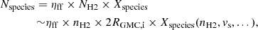
For the nonLTE analysis, we used the radiative-transfer code RADEX (van der Tak et al. 2007) via the Python package SpectralRadex2 (Holdship et al. 2021) using HNCO and SiO molecular data (Niedenhoff et al. 1995; Sahnoun et al. 2018; Balança et al. 2018) from the LAMDA database (Schöier et al. 2005). This allows us to account for how the gas density and temperature affect the excitation of the transitions in the nonLTE regime and to constrain three physical parameters of interest: gas density (nH2), gas temperature (Tkin), and the modeled species total column density (Nspecies) as well as the beam-filling factor (ηff).
We coupled the RADEX modeling with a Bayesian inference process to infer gas properties in order to properly sample the parameter space and obtain reliable uncertainties. The posterior probability distributions and the Bayesian evidence are derived with the nested sampling Monte Carlo algorithm MLFriends (Buchner 2016, 2019) using the UltraNest package3 (Buchner 2021). Similarly to the approach adopted by Huang et al. (2022), we assume priors of uniform or log-uniform distribution within the determined ranges (given in Table 4) and assume that the uncertainty on our measured intensities is Gaussian so that our likelihood is given by  where χ2 is the chi-squared statistic between our measured intensities and the RADEX output for a set of parameters θ.
In general, this analysis is confined by the assumption that all of the molecular transitions arise from a single and homogeneous gas component. This assumption can only offer an averaged view for the gas properties given the limited resolution of the observations, and the different critical densities of the available transitions. Despite that, if variations in gas temperature and density within each GMC region are not too steep, the inference should still be able to provide an indication of the average gas properties in the nonLTE study.
Figures 5–7 show the most representative cases of the posterior distribution among the sampled GMC regions. The remaining GMC cases are shown in Appendix D. The inferred gas properties from our GMCs are also listed in Table 5. Owing to the high quality of the ALCHEMI data and the ample number of transitions per species, most of the inferred gas properties are well constrained, which is a real benefit for further physical interpretation. In some circumstances, when RADEX fitting struggles to find a good solution, it may produce a solution where both nH2 and Tkin are at the edges of the parameter space, with either (low-nH2, high-Tkin) or (high-nH2, low-Tkin); this is a well-known degeneracy in the nH2–Tkin space. However, we did not find this to happen often. It is also worth noting that for some GMCs (e.g., GMC 6 and 1a), we did find cases with an optical depth –as predicted by RADEX-Bayesian analysis– of greater than unity for some of the SiO and/or HNCO transitions; this is compatible with our conclusion in Sect. 3.2 concerning non optically-thin LTE conditions.
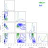 |
Fig. 5. Bayesian inference results for the gas properties traced by HNCO (green) and SiO (blue) of the GMC 1a region. The corner plots show the sampled distributions for each parameter, as displayed on the x-axis. The 1D distributions on the diagonal are the posterior distributions for each explored parameter; the remaining 2D distributions are the joint posterior for the corresponding parameter pairs on the x- and y-axes. |
Inferred gas properties traced by HNCO and SiO from the Bayesian inference processes over four selected regions across GMC1a-9a (Cols. 2–5).
Overall, HNCO appears to trace denser and cooler gas components compared to SiO across all the GMCs. On the other hand, the HNCO total column density is systematically lower than SiO. This suggests the two species trace distinctively different gas components. The total column density of each species is a function of gas density, emission-region size, and the fractional (relative to hydrogen) abundance of the species. If one assumes the beam-filling factors from HNCO and SiO are comparable (e.g., GMC 9a – Fig. 7), suggesting the emission region traced by both species is also comparable, this suggests that the fractional abundance of HNCO may be systematically smaller than that of SiO.
We also want to highlight that the gas temperature probed by SiO in most GMCs is hot (T > 400 K), hinting at the presence of shock heating. The two exceptions are GMC 2b and 8a, but both are still relatively warm (T > 200 K). If both require shocks, these suggest that the two groups of GMCs are simply at different post-shock cooling stages or that they are affected by different types of shocks.
There are a few GMCs that are particularly interesting. The gas traced by HNCO in GMC 1a points to a relatively low gas density (nH2 ∼ 103 cm−3) and high gas temperature (Tkin ∼ 230 K) compared to the rest of the GMCs traced by HNCO. The chemical modeling performed by Kelly et al. (2017) with a standard CRIR (= 1.3 × 10⁻¹⁷ s−1) showed that thermal sublimation cannot account for the HNCO enhancement with such low density for the gas and dust, which are not well coupled. However, in the case of NGC 253, multiple works have revealed high CRIR (∼10−14 − 10−11 s−1) for all GMCs (Holdship et al. 2021, 2022; Harada et al. 2021; Behrens et al. 2022). We discuss this further in Sect. 4.2.1. On the other hand, the gas traced by HNCO in GMC 7 points to a very low gas temperature (T ∼ 24 K) compared to all the other GMCs. In Sect. 4.2.2, we will further explore the possibility of thermal sublimation of HNCO at low temperatures. It is also interesting to compare GMCs of comparable temperature (Tkin > 50), as traced by HNCO in GMCs 4 and 6: here we find that GMC 6 has a higher abundance of HNCO (by a factor of two) than GMC 4. This was already suggested by the SLEDs shown in Sect. 3, where the HNCO SLED of GMC 6 showed greater brightness overall than GMC 4 despite their peaks all leaning towards a similar Eu. Finally, caution needs to be taken when interpreting our HNCO observations in GMC3, as although it appears that both gas density and gas temperature are constrained, in reality the nH2 peak and Tkin peak point to two degenerate sets of solutions. We list the best fit with best likelihood values in Table 5.
4.2. Chemical modeling
The RADEX and Bayesian inference process is “blind” to chemistry in so far as the chemistry behind each species is not taken into consideration: this may result in chemically unfeasible “best-fit” parameters. In this section, we therefore perform chemical modeling with the open-source time-dependent gas-grain UCLCHEM4 code (Holdship et al. 2017) in order to further disentangle and constrain the chemical origin of the observed HNCO and SiO emissions. UCLCHEM is a gas-grain chemical modeling code that incorporates user-defined chemical networks to produce chemical abundances along user-defined physics modules that can simulate a variety of physical conditions.
Compared to the older version of UCLCHEM used by Kelly et al. (2017), the latest UCLCHEM v3.1 includes updated chemistry and physics modules. Of importance to this study, UCLCHEM v3.1 includes an improved sputtering module in the parameterized C-shock model following Jiménez-Serra et al. (2008) as well as a three-phase chemistry where chemistry is computed for the gas phase, the grain surfaces, and the bulk ice. These improvements ensure a better treatment of the sputtering of refractory species such as Si-bearing molecules during the shock process. Aside from these technical differences, we also tailored our modeling for NGC 253, using a much higher CRIR than the standard galactic CRIR; that is, we used ζ = 103 − 5ζ0, while ζ0 = 1.3 × 10⁻¹⁷ s−1 is the standard galactic CRIR (Holdship et al. 2021, 2022; Harada et al. 2021; Behrens et al. 2022).
Chemical modeling with UCLCHEM typically involves two evolutionary stages. In our models, Stage 1 starts with the gas in diffuse atomic or ionic form and follows the chemical evolution of the gas and ices undergoing free-fall collapse up to a final density at the end of Stage 1. Based on the recipe described by Holdship et al. (2017), the initial elemental abundances are assumed to be solar. The temperature is set at 10 K. The output of this stage is a model of a typical quiescent molecular cloud. In our case, we assume that the gas-phase elemental abundance of Si has been depleted from solar level (Si/H ∼ 4.07 × 10⁻⁵, Lodders 2003) so that 99% of the Si is incorporated into the grain cores.
In Stage 2, we explore both shock (Sect. 4.2.1) and nonshock (Sect. 4.2.2) scenarios. For the shock models, we run a grid where we vary the following parameters: pre-shock gas density, post-shock gas temperature, shock velocity, and CRIR (or ζ). In Table 6, we list the parameter space explored in our Stage 2 chemical modeling analysis.
Parameter space explored in our chemical modeling.
For the post-shock gas, we assume that the post-shock gas temperature Tpost − shock is ∼50 K in order to cover most low temperatures measured in Sect. 4.1 as well as the dust temperatures (Td = 35 K) measured by Leroy et al. (2015) and the kinetic temperature (Tk ∼ 50 K) measured in less-dense gas (nH2 ∼ 104 cm−3) by Mangum et al. (2019).
4.2.1. Effects of the passage of C-shock(s) on the GMCs of NGC 253
The left panels of Figs. 8–11 show examples of our C-shock modelings. From our grid of models, we selected vs = 10 km s−1 and vs = 50 km s−1 as the most representative cases from our velocity grid for the slow and fast shock scenarios, respectively. In each figure, we present cases associated with a specified pre-shock density, such as nH2 = 103 cm−3, and each plot within the figure shows a case study with a specific combination of shock velocity (vs) and CRIR (ζ).
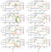 |
Fig. 8. Chemical abundances as a function of time for shocked (left panel) and nonshocked gas (right panel). The pre-shock gas density in the shock models and the gas density in nonshock models is 103 cm−3. The red dashed curve represents the temperature profile, with the temperature scale on the vertical axis on the right, also in red. For the shock models, within each panel we present from top to bottom: [shock velocity (vs) = 10 km s−1, CRIR (ζ) = 103ζ0], [shock velocity (vs) = 50 km s−1, CRIR (ζ) = 103ζ0], [shock velocity (vs) = 10 km s−1, CRIR (ζ) = 105ζ0], and [shock velocity (vs) = 50 km s−1, CRIR = 105ζ0]. The two selected temperatures for the nonshock models are 50 K and 200 K. The colored horizontal dashed lines indicate the lower limit of the species fractional abundances “measured” from our RADEX-Bayesian inference based on observational data and with an assumed hydrogen column density; see Sect. 5.1, for HNCO (blue) and SiO (orange), respectively. The fractional abundance values used are the minimum derived values among GMCs. For example, the SiO reference line (orange) is from values “measured” at GMC 7 as listed in Table 5, which provides the lowest “measured” fractional SiO abundance among all cases with gas density nH2 lower than 103 cm−3. |
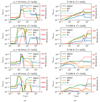 |
Fig. 10. As in Fig. 8, but for a pre-shock gas density in (a) and a gas density in (b) of 105 cm−3. The auxiliary line that indicates the lower limit of SiO (orange) fractional abundances “measured” from our RADEX-Bayesian inference is missing compared to Figs. 8 and 9 in the current case because observationally we do not find any GMC that is associated with such a high gas density. |
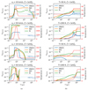 |
Fig. 11. As in Fig. 8 but for a pre-shock gas density in (a) and a gas density in (b) of 106 cm−3. The auxiliary line that indicates the lower limit of SiO (orange) fractional abundances “measured” from our RADEX-Bayesian inference is missing compared to Figs. 8 and 9 in the current case because observationally we do not find any GMC that is associated with such a high gas density. |
In each case, we plot the time evolution of the gas-phase molecular abundances of: HNCO (blue), SiO (orange), and Si (green). We also plot the gas temperature over time (red dashed) following the heating due to the shock as well as the minimum abundance imposed by the best fit from RADEX analysis (dashed horizontal lines), which is discussed in Sect. 5.1.
Overall, we see an enhancement of the SiO abundance during both slow (vs = 10 km s−1) and fast (vs = 50 km s−1) shocks, with the fast shocks leading to a much higher SiO abundance than achieved during the slow shocks. In the fast-shock condition, our main formation route of SiO depends on the gas density. In the lowest gas density case (nH2 = 103 cm−3), it is through the gas-phase reaction:
 (1)
(1)
while for higher density gas (nH2 ≥ 104 cm−3), the formation of SiO is mainly through the following gas-phase reaction:
 (2)
(2)
The main destruction route is via cosmic-ray induced photoreactions (expressed as “CRPHOT” in Eq. (3)) and/or other ionic particles (e.g., H3O+,  , H+) such as:
 (3)
(3)
 (4)
(4)
We also see that a high CRIR (ζ = 105ζ0) appears to further suppress the chemical abundances of SiO. In the higher density cases (nH2 ≥ 104 cm−3), this is due to the fact that the most efficient formation route for SiO is via neutral–neutral reactions of Si with OH (Eq. (2)). In a high-CRIR environment, both OH and Si are dissociated and ionized, respectively, more efficiently. In the lowest density case (nH2 = 103 cm−3), the formation route described in Eq. (1) is also much less efficient at higher CRIR.
It is clear that SiO is heavily enhanced by fast-shock sputtering across the densities studied. The inferred gas densities traced by SiO in Sect. 4.1 are nH2 ≤ 104 cm−3, and in these regimes the SiO enhancements are all dominated by fast-shock chemistry.
In contrast, in most cases, HNCO is enhanced in slow (vs = 10 km s−1) shocks rather than in fast shocks. Our main formation route of HNCO is on the dust grains followed by desorption:
 (5)
(5)
which is not viable when the ices are fully sputtered as in the fast-shock scenario, causing the associated low abundance of HNCO. Meanwhile, the destruction of HNCO is mainly through two gas-phase routes:
 (6)
(6)
 (7)
(7)
However, for cases with pre-shock gas density nH2 = 103 cm−3, none of the shock scenarios lead to sufficient HNCO to be detectable. The formation route described in Eq. (5) is never efficient enough at such low gas density. Nevertheless, our earlier analysis suggests some GMCs have a gas density of ∼nH2 = 103 cm−3; for example, GMC1a. The HNCO in this cloud cannot therefore be matched by any shock model. We speculate that this failure to reproduce a sufficient abundance of HNCO may be due to one of the following reasons: (1) An incomplete gas or surface HNCO network in our chemical modeling. (2) A best-likelihood case in the RADEX-inferred gas properties that is not necessarily chemically feasible; for example, a fit in the [nH2, Tkin, column density] space can be chemically unfeasible if the best-fit n and T cannot lead to abundances predicted by chemical modeling that lead back to the best fit of the column density. We investigate this possibility in Sect. 5.1. (3) Observationally, we may also be averaging over a multi-component gas that is denser and more compact within our beam. (4) HNCO may not be tracing the shocked gas in these low-density GMCs but may be enhanced by a different physical or chemical process. We explore this latter possibility in Sect. 4.2.2 with nonshock chemistry.
Finally, we note that Behrens et al. (2022) found that the inferred CRIR (ζ) is bimodal for GMC 1, with a main peak at 103ζ0 and a second peak at 10ζ0, although the model with low CRIR was considered likely to be unphysical (Behrens et al. 2022). Hence, in Fig. F.1 we also show the C-shock chemical modeling with a CRIR of ζ = ζ0 and ζ = 10ζ0. We indeed also find that with a lower CRIR, the HNCO abundance increases. However, it is still about ten times lower than the “observed” value, as further discussed in Sect. 5.1. The chemical model with low CRIR is still not able to explain our measurements toward GMC 1a.
4.2.2. Chemical evolution of nonshocked gas
As mentioned above, HNCO may be the product of thermal sublimation rather than shock sputtering as long as the gas and dust are well coupled. In order to test whether such a mechanism can efficiently boost the HNCO abundance in the gas where densities are as low as 103 cm−3 we use UCLCHEM to model the chemical evolution of a gas that is warmed up without the presence of shocks. This scenario could be representative of gas being warmed by the presence of star-forming processes (including outflows), and/or X-ray or cosmic rays. The physical module within UCLCHEM allows the temperature to increase over time.
We adopt two typical maximum temperatures inferred from HNCO observations, namely 50 K and 200 K, which capture most of the temperature ranges traced by HNCO as presented in Sect. 4.1, and the low temperatures measured in the literature as discussed earlier (Leroy et al. 2015; Mangum et al. 2019). We show the results of this modeling in the panels on the right in Figs. 8–11. From these figures, it is clear that neither HNCO nor SiO is sufficiently enhanced to match any of the observations. We test this scenario also with a lower CRIR (ζ = 1ζ0, Fig. F.2) and find that only cases with high temperatures (200 K) and dense gas (nH2 ≥ 104 cm−3) show a noticeable enhancement of HNCO abundance. However, none of the best-fit physical properties of any of our GMCs are consistent with such combinations of density and temperature. We also note that for GMCs (GMC 2b, 7) that probed even lower gas temperatures traced by HNCO than the lowest-T case tested here, of namely 50 K, given that none of the 50 K cases could reproduce sufficient HNCO, we expect no thermal sublimation to be feasible at these GMCs.
In summary, we do not find a reasonable nonshock model that can produce the high HNCO abundance we observe from the CMZ of NGC 253, particularly for gas densities as low as 103 cm−3.
5. Discussion
5.1. Are the RADEX-inferred gas properties chemically feasible?
The RADEX-inferred gas properties are the gas density (nH2), gas temperature (Tkin), and the column density of the species (NHNCO and NSiO). Chemical models, on the other hand, are provided with initial densities and temperatures and compute the chemical abundances of HNCO and SiO as a function of time. In this section, we attempt to determine whether the physical conditions inferred by our radiative-transfer inference analysis are compatible with the chemistry. The column density of a species can also be related to its chemical abundances predicted from chemical modeling, via the following on-the-spot approximation (Dyson & Williams 1997):
 (8)
(8)
where ηff is the beam filling factor, nH2 is the hydrogen column density, Xspecies is the fractional abundance of our species (with respect to the total number of atomic hydrogen nuclei), and RGMC, i is the radius of the GMC in consideration. We assume spherical clouds and approximate the line-of-sight depth with the plane-of-sky “diameter” of a GMC, namely 2 × RGMC, i, to be multiplied with the gas volume density for the estimate of column density. As the chemically predicted abundance is dependent on various factors, we express it as Xspecies(nH2, vs, ...) in the last equality. Nspecies, as defined using the above expression, must therefore be less than or equal to
 (9)
(9)
where the beam-filling factor, which may range between 0.0 and 1.0, was here assumed to be equal to 1 in order to obtain an upper limit on this estimate. The cloud diameter was taken to be the size of the beam, and we consider only the maximum abundance derived from the chemical models.
In other words, the above relationship determines whether the column density (estimated by the radiative-transfer analysis) can be reproduced by the chemical models computed with the parameters derived from the radiative-transfer modeling. The results of this verification are reported in Tables 7 and 8 for all our GMCs.
Comparison between the observations-inferred species column density and the chemical modelings for HNCO.
Comparison between the observation-inferred species column density and the chemical modelings for SiO.
Indeed, this verification confirms what we qualitatively found in Sect. 4.2.1, namely that in cases where the best fit for the pre-shock gas density is nH2 = 103 cm−3 (case solely for GMC 1a), we cannot reconcile the HNCO column density inferred by the radiative-transfer analysis with what is chemically feasible. For all the other cases, the relationship in Eq. (2) is satisfied.
In addition, we mentioned in Sect. 4.2.1 that we saw an enhancement of SiO abundance during both slow (vs = 10 km s−1) and fast (vs = 50 km s−1) shocks, but the fast shocks lead to a much higher SiO abundance than the slow shocks. More specifically, we find that the “enhanced” SiO abundance via slow shocks is insufficient compared to the RADEX-inferred results for the low -density case, that is nH2 = 103 cm−3 (top figure in the left panel of Fig. 8), using the same relation in Eq. (9). For the case where nH2 = 104 cm−3, although the predicted SiO resulting from slow shocks is sufficient, the high temperature measured from RADEX in these cases (GMC 4 and 6), T > 500 K, is not expected in the slow-shock models. This again reinforces the conclusion we drew in Sect. 4.2.1, that the abundance enhancement of SiO is dominated by fast-shock sputtering across the densities studied.
5.2. Physical interpretation of the gas properties
The current understanding of the shock chemistry as traced by HNCO and SiO is built upon many previous studies. The good correlation between HNCO and SiO revealed in Galactic dense molecular cores by Zinchenko et al. (2000) suggests that both species trace shocks, although the absence of HNCO in the higher velocity wings observed in the SiO spectral profile also hinted to the fact that high-velocity shock conditions may suppress the HNCO abundance. However, a follow-up survey over sources towards the Galactic center performed by Martín et al. (2008) reveals that HNCO can also be heavily destroyed by UV radiation in PDR regions (later also found in NGC 253 in Martín et al. 2009a). On the other hand, chemical modeling of HNCO and SiO in NGC 1068 performed by Kelly et al. (2017) confirmed that the HNCO abundance can be suppressed in high-velocity shocks due to the destruction of its precursor, the molecule NO. The analysis of HNCO and SiO in this work leads us to the conclusion that in at least most of the GMCs, HNCO and SiO emission can only be explained by the presence of shocks.
With this clear association between shock chemistry and our observed HNCO and SiO emission, the highly varying inferred gas properties across the GMCs may be the result of independent shock episodes. In this section, we use the physical properties inferred by the radiative transfer analysis coupled with the assumption that each GMC is subjected to the passage of a shock to estimate a rough timescale of the history of the shocks. Specifically, the “dissipation time” (τdissipation) is defined as the timescale when the velocity of ions and neutrals is equal, and can be viewed as the timescale over which the shock dissipates, or alternatively the shock-influence timescale. τdissipation is estimated by dividing the shock-dissipation distance described by Holdship et al. (2017) by the shock velocity, and depends solely on the pre-shock gas density. The larger the gas density, the shorter the timescale. From the post-shock temperature of the gas (derived from the UCLCHEM modeling), we can also roughly estimate the post-shock cooling timescale (τshock) relative to τdissipation. The two timescales can be qualitatively related in the following way:
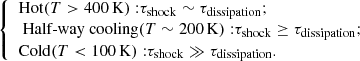 (10)
(10)
If the gas component remains hot, with the inferred gas temperature (Tkin) from the RADEX-Bayesian inference described in Sect. 4.1 being higher than 400 K, the region is possibly still under the influence of a shock episode, and therefore the age of the shock (τshock) is comparable to the dissipation timescale (τdissipation). The same logic is applied to the remaining two cases, that is, the half-way cooling and cold-gas conditions. Using Eq. (10), the inferred age of the shock (τshock) from each species for each GMC is listed in Col. 7 of Table 5.
Making one further assumption that the HNCO and SiO observed arise from the same shock episode, we can also take the intersection of both shock timescales and derive the joint shock timescale, τshock, joint. If there is no intersection between the SiO-shock timescale and HNCO-shock timescale, it may indeed be that the two molecules arise from different shock episodes, noting however that an “intersection” between the two timescales does not necessarily prove the opposite. The resulting “joint” shock timescale (τshock, joint) from this qualitative comparison is listed in the final column of Table 5 and displayed qualitatively in the bottom panel of Fig. 12. The τshock, joint of GMCs (GMC 4, 6, 7) from the inner CMZ tends to be smaller than that of the outer GMCs. In other words, this suggests the shocks in the inner GMCs tend to be younger (τshock, joint ∼ 103 yr) than those in the outer GMCs (τshock, joint ≥ 105 yr).
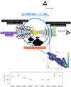 |
Fig. 12. Sketch (not to scale) of the three possible sources for star-formation induced shocks in the GMCs within the NGC 253 CMZ. We illustrate these three sources of shocks described in Sect. 5.3, and the relative layout of two possible line-of-sight (L.O.S.) orientations relative to the layout of shocked gas in each GMC. We assume the size of individual GMCs is comparable or larger than the ALCHEMI beam |

5.3. Origin(s) of the shocks
In this section, we qualitatively explore the possible origin(s) of the shocked environments probed via our HNCO and SiO observations. We propose three main possible scenarios that can lead to shocks within individual GMCs, as illustrated in Fig. 12: (1) shocks induced by outflowing material from “burst(s)” of star formation in the central region of each GMC (marked in black labels); (2) turbulent shocks induced by star-formation episodes in scattered locations within each GMC (marked with purple label); and (3) shocks induced by cloud–cloud collisions (marked with the orange label). In Fig. 12, we also place the relative layout of two possible line-of-sight (LOS) orientations relative to the physical setting in individual GMCs, which is not necessarily aligned with the galactic plane of NGC 253. We use the ALCHEMI beam (1″.6 ∼ 28 pc) as the GMC size –plotted as a solid blue circle– noting that of course GMCs will be of different sizes.
As the first potential source of shocks, the outflow can either induce: (1a) turbulent shocks on the working surface between the outflow and the ambient material (setup 1a in Fig. 12), or (1b) could also directly push the ambient material along the normal direction, and create “bow” shocks along the outflow (setup 1b in Fig. 12). Both setups are marked in black labels in Fig. 12.
For the second potential shock source, the HNCO and SiO emission could also be an ensemble from random locations and determining a timeline such as τshock, joint in Sect. 5.2 for the shock episodes would not be possible. This scenario is labeled in purple circles and text in Fig. 12.
Finally, we show the scenario where the shocks are caused by cloud–cloud collisions, which may occur especially near the outer GMCs (GMC 1a, 2b, 8a, 9a) because these regions are believed to be located at the intersections of a few dynamical orbits of the galaxy, including bar orbits and nuclear ring (see Harada et al. 2022; Humire et al. 2022, and reference therein). We note that cloud–cloud collisions in our own Galaxy and Large Magellanic Cloud (LMC) seem to occur at a moderate velocity ∼10 − 20 km s−1 (Li et al. 2018; Fukui et al. 2015) hinting at episodes of only weak shocks. However, cloud–cloud collisions at higher velocities can still occur at the intersections of dynamical orbits as proposed by Harada et al. (2019) for M83, and we expect a similar case applies to NGC 253.
We briefly discuss these scenarios below. García-Burillo et al. (2017) speculate on the presence of nondissociative shocks (traced by C2H) generated by the highly turbulent interfaces between the outflow and neighboring molecular gas in the circumnuclear disk (at scales of a few hundred parsecs) as well as in the starburst regions of the AGN-host galaxy NGC 1068. In our individual GMCs, although at the much smaller physical scales of a few parsecs, we may be witnessing a similar scenario, but on smaller scales. However, from our intensity maps, we do not see the extended morphology that suggests such structure (e.g., see Fig. 2 by García-Burillo et al. 2017); there is also the possibility that our spatial resolution with HNCO and SiO observations is just not sufficient to resolve such morphology within the beam-sized clump. Also, Holdship et al. (2021) showed that the enhanced C2H abundance could arise from either a high CRIR or shocks that occur within a timescale of 105 years, with the latter being less likely due to the timescale being very short. From our inferred shock timescales, the shock scenario does not appear to be entirely impossible. The other possible setup is that the star-formation-induced outflow can directly push against the ambient material along the normal or perpendicular direction, and create shocks along the outflow propagation. This creates a “single” shock episode that sweeps across the gas traced by both HNCO and SiO, possibly in different layers, because they seem to trace quite different gas densities in most of our GMCs. In this case, if the shocked gas components probed by HNCO and SiO can trace back to the same shock episode, we can further pin down the “age” of such shocks with τshock, joint as discussed in Sect. 5.2. The inferred age of this hypothesized “single” shock is listed in Table 5 for each GMC, and is also shown qualitatively in the bottom panel of Fig. 12. Of course, episodic shocks may be happening in random locations within the GMCs if star formation is ongoing. To determine the locations of such sporadic shock episodes, we would need observations of higher spatial resolution.
As a final note, globally the shock episodes throughout the CMZ may link to large-scale dynamical structures, such as an interface with the large-scale outflow. However, the spatial extent of our SiO and HNCO observations do not seem to be strongly tied with this possibility.
6. Conclusions
We analyzed six SiO transitions and eleven HNCO transitions imaged at GMC scales in the CMZ of NGC 253 with ALMA as part of the ALMA Large program ALCHEMI. Below, we briefly summarize our main conclusions:
-
Unlike the SiO SLEDs, the HNCO SLEDs differ in shape across the GMCs, hinting at substantial variations in at least the excitation conditions in the gas traced by HNCO across the GMCs.
-
Through radiative-transfer modeling using RADEX coupled with a Bayesian inference process, we successfully characterized the gas properties traced by these two molecular species and find them to be distinctively different.
-
Through radiative-transfer and chemical modeling, we find that the most likely physical scenario has the SiO emission arising from fast shocks while the HNCO emission arises from slow shocks.
-
We are able to infer the physical characteristics of the shocks traced by SiO and HNCO for each GMC, in particular the age of shocks traced by each species in each GMC.
-
We propose three possible shock scenarios that could explain the observed SiO and HNCO emission (see Fig. 12).
We conclude that the HNCO and SiO emission from the CMZ of NGC 253 are indeed associated with shocks potentially of different origins. Future higher spatial resolution observations are needed in order to further discern among those shock scenarios.
Acknowledgments
KYH, SV, JH, and MB are funded by the European Research Council (ERC) Advanced Grant MOPPEX 833460.vii. SGB acknowledges support from the research project PID2019-106027GA-C44 of the Spanish Ministerio de Ciencia e Innovación. L.C. acknowledges financial support through the Spanish grant PID2019-105552RB-C41 funded by MCIN/AEI/10.13039/501100011033. KYH and SV acknowledge the help from Marcus Keil and Ross O’Donoghue in working with UCLCHEM. KYH acknowledges assistance from Allegro, the European ALMA Regional Center node in the Netherlands. This paper makes use of the following ALMA data: ADS/JAO.ALMA#2017.1.00161.L and ADS/JAO.ALMA#2018.1.00162.S. ALMA is a partnership of ESO (representing its member states), NSF (USA) and NINS (Japan), together with NRC (Canada), MOST and ASIAA (Taiwan), and KASI (Republic of Korea), in cooperation with the Republic of Chile. The Joint ALMA Observatory is operated by ESO, AUI/NRAO and NAOJ.
References
- Aladro, R., Martín-Pintado, J., Martín, S., Mauersberger, R., & Bayet, E. 2011, A&A, 525, A89 [NASA ADS] [CrossRef] [EDP Sciences] [Google Scholar]
- Balança, C., Dayou, F., Faure, A., Wiesenfeld, L., & Feautrier, N. 2018, MNRAS, 479, 2692 [Google Scholar]
- Bayet, E., Lintott, C., Viti, S., et al. 2008, ApJ, 685, L35 [NASA ADS] [CrossRef] [Google Scholar]
- Behrens, E., Mangum, J. G., Holdship, J., et al. 2022, ApJ, 939, 119 [NASA ADS] [CrossRef] [Google Scholar]
- Bendo, G. J., Beswick, R. J., D’Cruze, M. J., et al. 2015, MNRAS, 450, L80 [NASA ADS] [CrossRef] [Google Scholar]
- Bolatto, A. D., Warren, S. R., Leroy, A. K., et al. 2013, Nature, 499, 450 [Google Scholar]
- Buchner, J. 2016, Stat. Comput., 26, 383 [Google Scholar]
- Buchner, J. 2019, PASP, 131, 108005 [Google Scholar]
- Buchner, J. 2021, J. Open Source Software, 6, 3001 [CrossRef] [Google Scholar]
- Canelo, C. M., Bronfman, L., Mendoza, E., et al. 2021, MNRAS, 504, 4428 [NASA ADS] [CrossRef] [Google Scholar]
- Carvajal, M., Favre, C., Kleiner, I., et al. 2019, A&A, 627, A65 [NASA ADS] [CrossRef] [EDP Sciences] [Google Scholar]
- Colzi, L., Rivilla, V. M., Beltrán, M. T., et al. 2021, A&A, 653, A129 [NASA ADS] [CrossRef] [EDP Sciences] [Google Scholar]
- Dyson, J. E., & Williams, D. A. 1997, The Physics of the Interstellar Medium (Bristol: Institute of Physics Publishing) [CrossRef] [Google Scholar]
- Endres, C. P., Schlemmer, S., Schilke, P., Stutzki, J., & Müller, H. S. P. 2016, J. Mol. Spectrosc., 327, 95 [NASA ADS] [CrossRef] [Google Scholar]
- Fedoseev, G., Ioppolo, S., Zhao, D., Lamberts, T., & Linnartz, H. 2015, MNRAS, 446, 439 [NASA ADS] [CrossRef] [Google Scholar]
- Fukui, Y., Harada, R., Tokuda, K., et al. 2015, ApJ, 807, L4 [NASA ADS] [CrossRef] [Google Scholar]
- Gao, Y., & Solomon, P. M. 2004, ApJ, 606, 271 [NASA ADS] [CrossRef] [Google Scholar]
- García-Burillo, S., Martín-Pintado, J., Fuente, A., & Neri, R. 2000, A&A, 355, 499 [NASA ADS] [Google Scholar]
- García-Burillo, S., Martín-Pintado, J., Fuente, A., Usero, A., & Neri, R. 2002, ApJ, 575, L55 [CrossRef] [Google Scholar]
- García-Burillo, S., Usero, A., Fuente, A., et al. 2010, A&A, 519, A2 [NASA ADS] [CrossRef] [EDP Sciences] [Google Scholar]
- García-Burillo, S., Viti, S., Combes, F., et al. 2017, A&A, 608, A56 [Google Scholar]
- Gerin, M., Goicoechea, J. R., Pety, J., & Hily-Blant, P. 2009, A&A, 494, 977 [NASA ADS] [CrossRef] [EDP Sciences] [Google Scholar]
- Gorai, P., Bhat, B., Sil, M., et al. 2020, ApJ, 895, 86 [Google Scholar]
- Haasler, D., Rivilla, V. M., Martín, S., et al. 2022, A&A, 659, A158 [CrossRef] [EDP Sciences] [Google Scholar]
- Harada, N., Sakamoto, K., Martín, S., et al. 2019, ApJ, 884, 100 [NASA ADS] [CrossRef] [Google Scholar]
- Harada, N., Martín, S., Mangum, J. G., et al. 2021, ApJ, 923, 24 [NASA ADS] [CrossRef] [Google Scholar]
- Harada, N., Martín, S., Mangum, J. G., et al. 2022, ApJ, 938, 80 [NASA ADS] [CrossRef] [Google Scholar]
- Hernández-Gómez, A., Sahnoun, E., Caux, E., et al. 2019, MNRAS, 483, 2014 [CrossRef] [Google Scholar]
- Holdship, J., Viti, S., Jiménez-Serra, I., Makrymallis, A., & Priestley, F. 2017, AJ, 154, 38 [NASA ADS] [CrossRef] [Google Scholar]
- Holdship, J., Viti, S., Martín, S., et al. 2021, A&A, 654, A55 [NASA ADS] [CrossRef] [EDP Sciences] [Google Scholar]
- Holdship, J., Mangum, J. G., Viti, S., et al. 2022, ApJ, 931, 89 [NASA ADS] [CrossRef] [Google Scholar]
- Huang, K. Y., Viti, S., Holdship, J., et al. 2022, A&A, 666, A102 [NASA ADS] [CrossRef] [EDP Sciences] [Google Scholar]
- Humire, P. K., Henkel, C., Hernández-Gómez, A., et al. 2022, A&A, 663, A33 [NASA ADS] [CrossRef] [EDP Sciences] [Google Scholar]
- Hüttemeister, S., Dahmen, G., Mauersberger, R., et al. 1998, A&A, 334, 646 [NASA ADS] [Google Scholar]
- Jiménez-Serra, I., Caselli, P., Martín-Pintado, J., & Hartquist, T. W. 2008, A&A, 482, 549 [NASA ADS] [CrossRef] [EDP Sciences] [Google Scholar]
- Kauffmann, J., Goldsmith, P. F., Melnick, G., et al. 2017, A&A, 605, L5 [NASA ADS] [CrossRef] [EDP Sciences] [Google Scholar]
- Kelly, G., Viti, S., García-Burillo, S., et al. 2017, A&A, 597, A11 [NASA ADS] [CrossRef] [EDP Sciences] [Google Scholar]
- Krieger, N., Bolatto, A. D., Walter, F., et al. 2019, ApJ, 881, 43 [NASA ADS] [CrossRef] [Google Scholar]
- Krips, M., Neri, R., García-Burillo, S., et al. 2008, ApJ, 677, 262 [NASA ADS] [CrossRef] [Google Scholar]
- Lehmer, B. D., Wik, D. R., Hornschemeier, A. E., et al. 2013, ApJ, 771, 134 [NASA ADS] [CrossRef] [Google Scholar]
- Leroy, A. K., Bolatto, A. D., Ostriker, E. C., et al. 2015, ApJ, 801, 25 [NASA ADS] [CrossRef] [Google Scholar]
- Leroy, A. K., Bolatto, A. D., Ostriker, E. C., et al. 2018, ApJ, 869, 126 [NASA ADS] [CrossRef] [Google Scholar]
- Levy, R. C., Bolatto, A. D., Leroy, A. K., et al. 2022, ApJ, 935, 19 [NASA ADS] [CrossRef] [Google Scholar]
- Li, Q., Tan, J. C., Christie, D., Bisbas, T. G., & Wu, B. 2018, PASJ, 70, S56 [NASA ADS] [Google Scholar]
- Lodders, K. 2003, ApJ, 591, 1220 [Google Scholar]
- López-Sepulcre, A., Jaber, A. A., Mendoza, E., et al. 2015, MNRAS, 449, 2438 [CrossRef] [Google Scholar]
- Mangum, J. G., Ginsburg, A. G., Henkel, C., et al. 2019, ApJ, 871, 170 [NASA ADS] [CrossRef] [Google Scholar]
- Martín, S., Requena-Torres, M. A., Martín-Pintado, J., & Mauersberger, R. 2008, ApJ, 678, 245 [CrossRef] [Google Scholar]
- Martín, S., Martín-Pintado, J., & Viti, S. 2009a, ApJ, 706, 1323 [Google Scholar]
- Martín, S., Martín-Pintado, J., & Mauersberger, R. 2009b, ApJ, 694, 610 [CrossRef] [Google Scholar]
- Martín, S., Kohno, K., Izumi, T., et al. 2015, A&A, 573, A116 [NASA ADS] [CrossRef] [EDP Sciences] [Google Scholar]
- Martín, S., Mangum, J. G., Harada, N., et al. 2021, A&A, 656, A46 [NASA ADS] [CrossRef] [EDP Sciences] [Google Scholar]
- Martín-Pintado, J., de Vicente, P., Fuente, A., & Planesas, P. 1997, ApJ, 482, L45 [NASA ADS] [CrossRef] [Google Scholar]
- McCarthy, P. J., van Breugel, W., & Heckman, T. 1987, AJ, 93, 264 [NASA ADS] [CrossRef] [Google Scholar]
- McCormick, A., Veilleux, S., & Rupke, D. S. N. 2013, ApJ, 774, 126 [NASA ADS] [CrossRef] [Google Scholar]
- Meier, D. S., & Turner, J. L. 2005, ApJ, 618, 259 [NASA ADS] [CrossRef] [Google Scholar]
- Meier, D. S., & Turner, J. L. 2012, ApJ, 755, 104 [NASA ADS] [CrossRef] [Google Scholar]
- Meier, D. S., Walter, F., Bolatto, A. D., et al. 2015, ApJ, 801, 63 [NASA ADS] [CrossRef] [Google Scholar]
- Mendoza, E., Lefloch, B., López-Sepulcre, A., et al. 2014, MNRAS, 445, 151 [NASA ADS] [CrossRef] [Google Scholar]
- Müller, H. S. P., Thorwirth, S., Roth, D. A., & Winnewisser, G. 2001, A&A, 370, L49 [Google Scholar]
- Müller, H. S. P., Schlöder, F., Stutzki, J., & Winnewisser, G. 2005, J. Mol. Struct., 742, 215 [Google Scholar]
- Müller-Sánchez, F., González-Martín, O., Fernández-Ontiveros, J. A., Acosta-Pulido, J. A., & Prieto, M. A. 2010, ApJ, 716, 1166 [CrossRef] [Google Scholar]
- Nazari, P., van Gelder, M. L., van Dishoeck, E. F., et al. 2021, A&A, 650, A150 [EDP Sciences] [Google Scholar]
- Niedenhoff, M., Yamada, K. M. T., Belov, S. P., & Winnewisser, G. 1995, J. Mol. Spectrosc., 174, 151 [NASA ADS] [CrossRef] [Google Scholar]
- Pety, J., Guzmán, V. V., Orkisz, J. H., et al. 2017, A&A, 599, A98 [NASA ADS] [CrossRef] [EDP Sciences] [Google Scholar]
- Podio, L., Codella, C., Lefloch, B., et al. 2017, MNRAS, 470, L16 [Google Scholar]
- Rekola, R., Richer, M. G., McCall, M. L., et al. 2005, MNRAS, 361, 330 [NASA ADS] [CrossRef] [Google Scholar]
- Rizzo, J. R., Cernicharo, J., & García-Miró, C. 2021, ApJS, 253, 44 [NASA ADS] [CrossRef] [Google Scholar]
- Rodríguez-Fernández, N. J., Tafalla, M., Gueth, F., & Bachiller, R. 2010, A&A, 516, A98 [Google Scholar]
- Sahnoun, E., Wiesenfeld, L., Hammami, K., & Jaidane, N. 2018, J. Phys. Chem. A, 122, 3004 [NASA ADS] [CrossRef] [Google Scholar]
- Sakamoto, K., Mao, R.-Q., Matsushita, S., et al. 2011, ApJ, 735, 19 [CrossRef] [Google Scholar]
- Savage, C., & Ziurys, L. M. 2004, ApJ, 616, 966 [NASA ADS] [CrossRef] [Google Scholar]
- Schilke, P., Walmsley, C. M., & Pineau des Forets, G., & Flower, D. R., 1997, A&A, 321, 293 [Google Scholar]
- Schöier, F. L., van der Tak, F. F. S., van Dishoeck, E. F., & Black, J. H. 2005, A&A, 432, 369 [Google Scholar]
- Strickland, D. K., Heckman, T. M., Weaver, K. A., & Dahlem, M. 2000, AJ, 120, 2965 [NASA ADS] [CrossRef] [Google Scholar]
- Strickland, D. K., Heckman, T. M., Weaver, K. A., Hoopes, C. G., & Dahlem, M. 2002, ApJ, 568, 689 [NASA ADS] [CrossRef] [Google Scholar]
- Tafalla, M., Usero, A., & Hacar, A. 2021, A&A, 646, A97 [NASA ADS] [CrossRef] [EDP Sciences] [Google Scholar]
- Turner, B. E. 1985, ApJ, 299, 312 [NASA ADS] [CrossRef] [Google Scholar]
- Turner, J. L., & Ho, P. T. P. 1985, ApJ, 299, L77 [NASA ADS] [CrossRef] [Google Scholar]
- Usero, A., García-Burillo, S., Martín-Pintado, J., Fuente, A., & Neri, R. 2006, A&A, 448, 457 [NASA ADS] [CrossRef] [EDP Sciences] [Google Scholar]
- van der Tak, F. F. S., Black, J. H., Schöier, F. L., Jansen, D. J., & van Dishoeck, E. F. 2007, A&A, 468, 627 [NASA ADS] [CrossRef] [EDP Sciences] [Google Scholar]
- Velilla Prieto, L., Sánchez Contreras, C., Cernicharo, J., et al. 2015, A&A, 575, A84 [CrossRef] [EDP Sciences] [Google Scholar]
- Velilla Prieto, L., Sánchez Contreras, C., Cernicharo, J., et al. 2017, A&A, 597, A25 [NASA ADS] [CrossRef] [EDP Sciences] [Google Scholar]
- Viti, S. 2017, A&A, 607, A118 [NASA ADS] [CrossRef] [EDP Sciences] [Google Scholar]
- Walter, F., Bolatto, A. D., Leroy, A. K., et al. 2017, ApJ, 835, 265 [NASA ADS] [CrossRef] [Google Scholar]
- Westmoquette, M. S., Smith, L. J., Gallagher, J. S. I., 2011, MNRAS, 414, 3719 [NASA ADS] [CrossRef] [Google Scholar]
- Zeng, S., Jiménez-Serra, I., Rivilla, V. M., et al. 2018, MNRAS, 478, 2962 [Google Scholar]
- Zinchenko, I., Henkel, C., & Mao, R. Q. 2000, A&A, 361, 1079 [NASA ADS] [Google Scholar]
Appendix A: Spectra of molecular transitions
In this section, we show the spectra from all the SiO (Fig. A.1) and HNCO (Fig. A.2) transitions used in the current work. The spectra are extracted from the representative region - GMC 6 - as listed in Table 2.
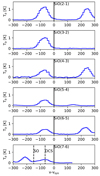 |
Fig. A.1. Spectra extracted from GMC 6, for all SiO transitions. used in this work. The solid vertical line marks the rest frequency of each transition, and the dashed vertical line(s) the adjacent or blending line. |
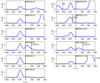 |
Fig. A.2. Spectra extracted from GMC 6, for all HNCO transitions. used in this work. The solid vertical line marks the reference target transition with respect to the systemic velocity of ngc 253 (vsys = 258.8 km s-1), and the dashed vertical line the adjacent or blending line. |
Appendix B: Additional intensity maps
In this section, we display the velocity-integrated intensity maps for the remaining HNCO and SiO transition that are not shown in the main text.
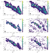 |
Fig. B.1. Remaining velocity-integrated line intensities in [K km s-1] of HNCO transitions: (5-4)/(6-5)/(8-7)/(9-8)/100,10-90,9/(13-12), ordered accordingly from (a) to (f). We note that the HNCO (8-7) transition is close to the 183 GHz water line. |
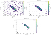 |
Fig. B.2. Velocity-integrated line intensities in [K km s-1] of HNCO (13-12), (14-13), and (15-14) transitions. |
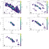 |
Fig. B.3. Velocity-integrated line intensities in [K km s-1] of the remaining SiO transitions: SiO (3-2) up to (7-6). |
Appendix C: Line intensity ratio maps
In this section, we display the intensity ratio maps described in Sect. 3.2.
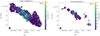 |
Fig. C.1. Line-intensity ratio maps of two selected pairs: SiO(2-1) and HNCO (40,4-30,3), and SiO(7-6) and HNCO 10(0,10-90,9). |
Appendix D: Additional corner plots for GMC2b/3/5/9a/10
The RADEX-Bayesian inference results for the remaining GMCs: GMC 2b, 3, 4, 6, and 8a.
Appendix E: Comparison of the predicted intensity from the RADEX-Bayesian inference analysis with observed values: A posterior predictive check (PPC)
We perform a posterior predictive check for the inferred gas properties in Sect. 4.1 from the coupled RADEX and Bayesian inference process. This is to verify that our posterior distribution produces a distribution for the data that is consistent with the actual data, which is the velocity-integrated intensity in our case. We sample the predicted line intensities from our posterior between the 16th and 84th percentiles, and plot these against the observed line intensities. The comparisons are shown in Fig. E.1-E.4.
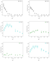 |
Fig. E.1. The posterior predictive checks (PPCs) of all HNCO transitions, GMC 1a-6, ordered accordingly from (a) to (f). The observed line intensity is in marker with uncertainty in line segment. The predicted line intensity is in colored band overlaid in the background. |
 |
Fig. E.2. The posterior predictive checks (PPCs) of all HNCO transitions, GMC 7-10, ordered accordingly from (a) to (d). The observed line intensity is in marker with uncertainty in line segment. The predicted line intensity from RADEX-Bayesian analysis is in colored band overlaid in the background. |
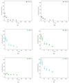 |
Fig. E.3. The posterior predictive checks (PPCs) of all SiO transitions, GMC 1a-6, ordered accordingly from (a) to (f). The observed line intensity is in marker with uncertainty in line segment. The predicted line intensity from RADEX-Bayesian analysis is in colored band overlaid in the background. |
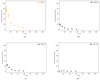 |
Fig. E.4. The posterior predictive checks (PPCs) of all SiO transitions, GMC 7-10, ordered accordingly from (a) to (d). The observed line intensity is in marker with uncertainty in line segment. The predicted line intensity from RADEX-Bayesian analysis is in colored band overlaid in the background. |
Appendix F: Additional cases explored in chemical modeling
Figure F.1 shows the outputs of the extra chemical models we performed, where we varied the CRIR. With a standard galactic CRIR (ζ = ζ0, top panel in Fig. F.1) in the slow-shock scenario at the low-density of n = 103 cm-3) case, it is possible to enhance the HNCO abundance to a higher level, which is in contrast with other higher CRIR conditions (lower panels in Fig. F.1). However, we note this enhancement is still insufficient to achieve the lower limit imposed by the RADEX result (blue dashed horizontal line).
Figure F.2 shows the nonshock models with ζ = ζ0 for temperatures of T = 50 K (left panel) and T = 200 K (right panel), respectively. At higher gas density (n ≥ 104 cm-3), it shows HNCO abundance can also be enhanced in the absence of shocks with low CRIR, ζ = ζ0, and high temperature T = 200 K.
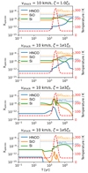 |
Fig. F.1. Alternative cases with pre-shock gas density nH2 = 103 cm-3 in a slow shock scenario (vs = 10 km/s, where we compare cases of CRIR from 1ζ0 (top) to 105ζ0 (bottom). It is clear that an higher CRIR could further suppress the HNCO abundance enhanced via slow shocks. |
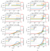 |
Fig. F.2. Alternative chemical models without shocks with temperature = 50 K (left panel) and with temperature = 200 K (right panel) using a low CRIR of ζ = 1ζ0. At this cooler temperature, even with low CRIR, the HNCO abundance cannot be enhanced to a reasonable level to be matched with observational results. |
All Tables
Inferred gas properties traced by HNCO and SiO from the Bayesian inference processes over four selected regions across GMC1a-9a (Cols. 2–5).
Comparison between the observations-inferred species column density and the chemical modelings for HNCO.
Comparison between the observation-inferred species column density and the chemical modelings for SiO.
All Figures
|
Fig. 1. Velocity-integrated line intensities in [K km s−1] of the HNCO transitions: (40, 4–30, 3) and (100, 10–90, 9), in (a) and (b), respectively. These two transitions are representative of the drastic variation in the trend of brightness from outer to inner GMCs. The rest of the HNCO line intensity maps are provided in Appendix B. The studied GMC regions as listed in Table 2 are labeled in white text on the map. The ALCHEMI |
| In the text | |
|
Fig. 2. Velocity-integrated line intensities of the SiO (2–1) transition in [K km s−1]. The remaining SiO line-intensity maps are provided in Appendix B. The studied GMC regions as listed in Table 2 are labeled in white text on the map. The ALCHEMI |
| In the text | |
|
Fig. 3. SLED over all available energy levels of HNCO. The units are in [K km s−1]. The GMCs are categorized by the “shape” of the ladders and are labeled accordingly in different colors as described in Sect. 3: GMC3/6 (in cyan), GMC4/5 (in green), and GMC7 (in orange), and the outer GMCs: GMC 1a, 1b, 2a, 2b, 8a, 9a, and 10 (in black). The “shadowed” markers in each diagram represent nondetected points, and are displayed with an upper limit only. |
| In the text | |
|
Fig. 4. As in Fig. 3, but for SiO. |
| In the text | |
|
Fig. 5. Bayesian inference results for the gas properties traced by HNCO (green) and SiO (blue) of the GMC 1a region. The corner plots show the sampled distributions for each parameter, as displayed on the x-axis. The 1D distributions on the diagonal are the posterior distributions for each explored parameter; the remaining 2D distributions are the joint posterior for the corresponding parameter pairs on the x- and y-axes. |
| In the text | |
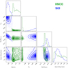 |
Fig. 6. As in Fig. 5, but for GMC7, as a representative region for the inner GMCs. |
| In the text | |
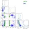 |
Fig. 7. As in Fig. 5, but for GMC9a, as a representative region for the outer GMCs. |
| In the text | |
|
Fig. 8. Chemical abundances as a function of time for shocked (left panel) and nonshocked gas (right panel). The pre-shock gas density in the shock models and the gas density in nonshock models is 103 cm−3. The red dashed curve represents the temperature profile, with the temperature scale on the vertical axis on the right, also in red. For the shock models, within each panel we present from top to bottom: [shock velocity (vs) = 10 km s−1, CRIR (ζ) = 103ζ0], [shock velocity (vs) = 50 km s−1, CRIR (ζ) = 103ζ0], [shock velocity (vs) = 10 km s−1, CRIR (ζ) = 105ζ0], and [shock velocity (vs) = 50 km s−1, CRIR = 105ζ0]. The two selected temperatures for the nonshock models are 50 K and 200 K. The colored horizontal dashed lines indicate the lower limit of the species fractional abundances “measured” from our RADEX-Bayesian inference based on observational data and with an assumed hydrogen column density; see Sect. 5.1, for HNCO (blue) and SiO (orange), respectively. The fractional abundance values used are the minimum derived values among GMCs. For example, the SiO reference line (orange) is from values “measured” at GMC 7 as listed in Table 5, which provides the lowest “measured” fractional SiO abundance among all cases with gas density nH2 lower than 103 cm−3. |
| In the text | |
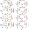 |
Fig. 9. As in Fig. 8, but for a pre-shock gas density in (a) and a gas density in (b) of 104 cm−3. |
| In the text | |
|
Fig. 10. As in Fig. 8, but for a pre-shock gas density in (a) and a gas density in (b) of 105 cm−3. The auxiliary line that indicates the lower limit of SiO (orange) fractional abundances “measured” from our RADEX-Bayesian inference is missing compared to Figs. 8 and 9 in the current case because observationally we do not find any GMC that is associated with such a high gas density. |
| In the text | |
|
Fig. 11. As in Fig. 8 but for a pre-shock gas density in (a) and a gas density in (b) of 106 cm−3. The auxiliary line that indicates the lower limit of SiO (orange) fractional abundances “measured” from our RADEX-Bayesian inference is missing compared to Figs. 8 and 9 in the current case because observationally we do not find any GMC that is associated with such a high gas density. |
| In the text | |
|
Fig. 12. Sketch (not to scale) of the three possible sources for star-formation induced shocks in the GMCs within the NGC 253 CMZ. We illustrate these three sources of shocks described in Sect. 5.3, and the relative layout of two possible line-of-sight (L.O.S.) orientations relative to the layout of shocked gas in each GMC. We assume the size of individual GMCs is comparable or larger than the ALCHEMI beam |
| In the text | |
|
Fig. A.1. Spectra extracted from GMC 6, for all SiO transitions. used in this work. The solid vertical line marks the rest frequency of each transition, and the dashed vertical line(s) the adjacent or blending line. |
| In the text | |
|
Fig. A.2. Spectra extracted from GMC 6, for all HNCO transitions. used in this work. The solid vertical line marks the reference target transition with respect to the systemic velocity of ngc 253 (vsys = 258.8 km s-1), and the dashed vertical line the adjacent or blending line. |
| In the text | |
|
Fig. B.1. Remaining velocity-integrated line intensities in [K km s-1] of HNCO transitions: (5-4)/(6-5)/(8-7)/(9-8)/100,10-90,9/(13-12), ordered accordingly from (a) to (f). We note that the HNCO (8-7) transition is close to the 183 GHz water line. |
| In the text | |
|
Fig. B.2. Velocity-integrated line intensities in [K km s-1] of HNCO (13-12), (14-13), and (15-14) transitions. |
| In the text | |
|
Fig. B.3. Velocity-integrated line intensities in [K km s-1] of the remaining SiO transitions: SiO (3-2) up to (7-6). |
| In the text | |
|
Fig. C.1. Line-intensity ratio maps of two selected pairs: SiO(2-1) and HNCO (40,4-30,3), and SiO(7-6) and HNCO 10(0,10-90,9). |
| In the text | |
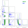 |
Fig. D.1. Same as Fig. 5 but for GMC2b. |
| In the text | |
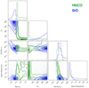 |
Fig. D.2. Same as Fig. 5 but for GMC3. |
| In the text | |
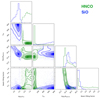 |
Fig. D.3. Same as Fig. 5 but for GMC4. |
| In the text | |
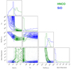 |
Fig. D.4. Same as Fig. 5 but for GMC6. |
| In the text | |
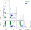 |
Fig. D.5. Same as Fig. 5 but for GMC8a. |
| In the text | |
|
Fig. E.1. The posterior predictive checks (PPCs) of all HNCO transitions, GMC 1a-6, ordered accordingly from (a) to (f). The observed line intensity is in marker with uncertainty in line segment. The predicted line intensity is in colored band overlaid in the background. |
| In the text | |
|
Fig. E.2. The posterior predictive checks (PPCs) of all HNCO transitions, GMC 7-10, ordered accordingly from (a) to (d). The observed line intensity is in marker with uncertainty in line segment. The predicted line intensity from RADEX-Bayesian analysis is in colored band overlaid in the background. |
| In the text | |
|
Fig. E.3. The posterior predictive checks (PPCs) of all SiO transitions, GMC 1a-6, ordered accordingly from (a) to (f). The observed line intensity is in marker with uncertainty in line segment. The predicted line intensity from RADEX-Bayesian analysis is in colored band overlaid in the background. |
| In the text | |
|
Fig. E.4. The posterior predictive checks (PPCs) of all SiO transitions, GMC 7-10, ordered accordingly from (a) to (d). The observed line intensity is in marker with uncertainty in line segment. The predicted line intensity from RADEX-Bayesian analysis is in colored band overlaid in the background. |
| In the text | |
|
Fig. F.1. Alternative cases with pre-shock gas density nH2 = 103 cm-3 in a slow shock scenario (vs = 10 km/s, where we compare cases of CRIR from 1ζ0 (top) to 105ζ0 (bottom). It is clear that an higher CRIR could further suppress the HNCO abundance enhanced via slow shocks. |
| In the text | |
|
Fig. F.2. Alternative chemical models without shocks with temperature = 50 K (left panel) and with temperature = 200 K (right panel) using a low CRIR of ζ = 1ζ0. At this cooler temperature, even with low CRIR, the HNCO abundance cannot be enhanced to a reasonable level to be matched with observational results. |
| In the text | |
Current usage metrics show cumulative count of Article Views (full-text article views including HTML views, PDF and ePub downloads, according to the available data) and Abstracts Views on Vision4Press platform.
Data correspond to usage on the plateform after 2015. The current usage metrics is available 48-96 hours after online publication and is updated daily on week days.
Initial download of the metrics may take a while.