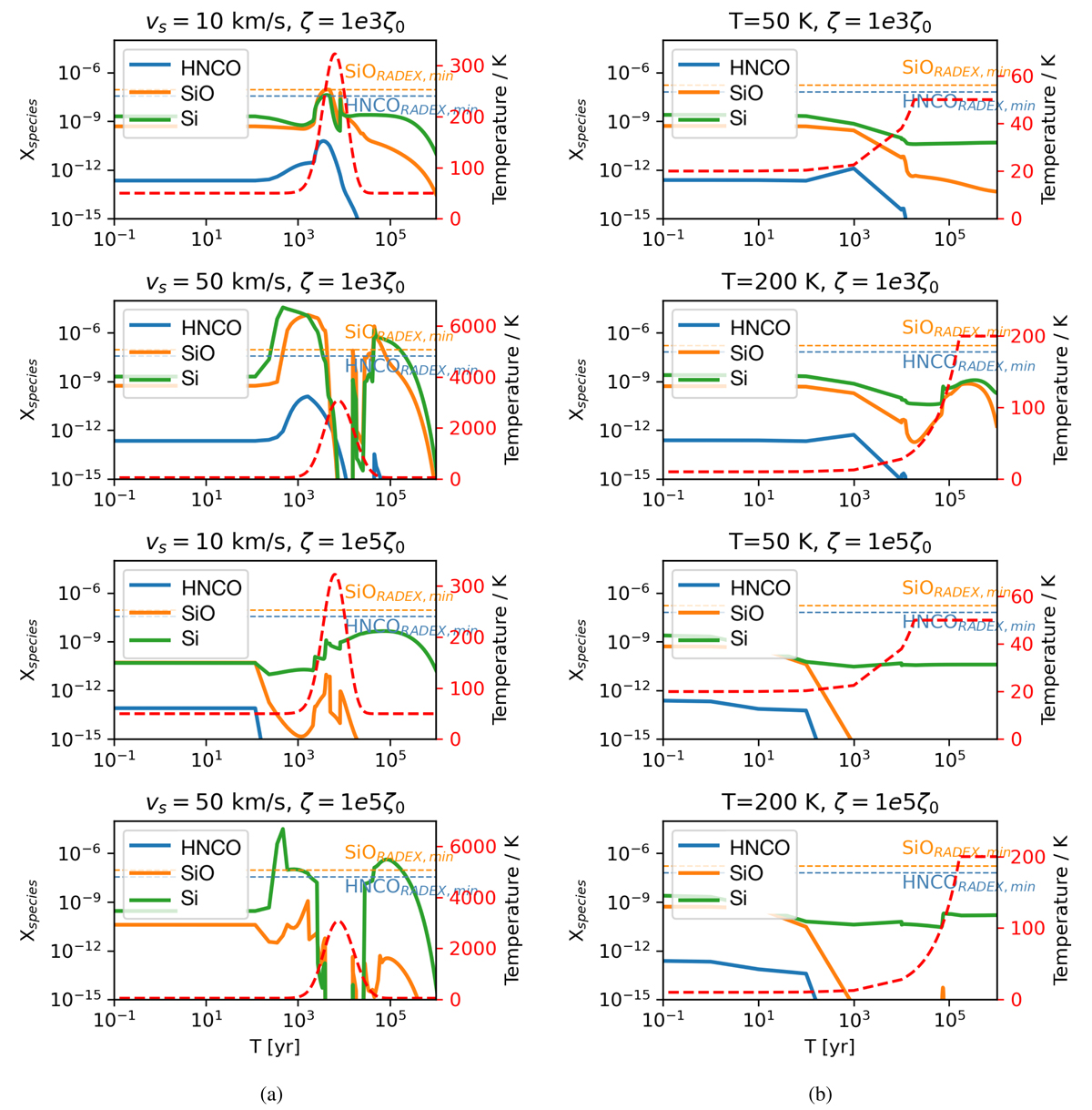
Chemical abundances as a function of time for shocked (left panel) and nonshocked gas (right panel). The pre-shock gas density in the shock models and the gas density in nonshock models is 10³ cm⁻³. The red dashed curve represents the temperature profile, with the temperature scale on the vertical axis on the right, also in red. For the shock models, within each panel we present from top to bottom: [shock velocity (v_s) = 10 km s⁻¹, CRIR (ζ) = 10³ζ₀], [shock velocity (v_s) = 50 km s⁻¹, CRIR (ζ) = 10³ζ₀], [shock velocity (v_s) = 10 km s⁻¹, CRIR (ζ) = 10⁵ζ₀], and [shock velocity (v_s) = 50 km s⁻¹, CRIR = 10⁵ζ₀]. The two selected temperatures for the nonshock models are 50 K and 200 K. The colored horizontal dashed lines indicate the lower limit of the species fractional abundances “measured” from our RADEX-Bayesian inference based on observational data and with an assumed hydrogen column density; see Sect. 5.1, for HNCO (blue) and SiO (orange), respectively. The fractional abundance values used are the minimum derived values among GMCs. For example, the SiO reference line (orange) is from values “measured” at GMC 7 as listed in Table 5, which provides the lowest “measured” fractional SiO abundance among all cases with gas density n_H2 lower than 10³ cm⁻³.