Complex organic molecules towards the central molecular zone of NGC 253

M. Bouvier; S. Viti; J. G. Mangum; C. Eibensteiner; E. Behrens; V. M. Rivilla; Á. López-Gallifa; S. Martín; N. Harada; S. Muller; L. Colzi; K. Sakamoto

doi:10.1051/0004-6361/202554420

Home

All issues

Volume 698 (May 2025)

A&A, 698 (2025) A261

Full HTML

Open Access

Issue		A&A Volume 698, May 2025


Article Number		A261
Number of page(s)		22
Section		Extragalactic astronomy
DOI		https://doi.org/10.1051/0004-6361/202554420
Published online		20 June 2025

A&A, 698, A261 (2025)

Complex organic molecules towards the central molecular zone of NGC 253

M. Bouvier¹^⋆, S. Viti¹^,2^,3, J. G. Mangum⁴, C. Eibensteiner⁴^,⋆⋆, E. Behrens⁵^,4, V. M. Rivilla⁶, Á. López-Gallifa⁶, S. Martín⁷^,8, N. Harada⁹^,10, S. Muller¹¹, L. Colzi⁶ and K. Sakamoto¹²

¹ Leiden Observatory, Leiden University, PO Box 9513, 2300 RA Leiden, The Netherlands
² Transdisciplinary Research Area (TRA) ‘Matter’/Argelander-Institut für Astronomie, University of Bonn, Germany
³ Physics and Astronomy, University College London, UK
⁴ National Radio Astronomy Observatory, 520 Edgemont Road, Charlottesville, VA 22903-2475, USA
⁵ Department of Astronomy, University of Virginia, PO Box 400325, 530 McCormick Road, Charlottesville, VA 22904-4325, USA
⁶ Centro de Astrobiología (CAB), CSIC-INTA, Carretera de Ajalvir km 4, Torrejón de Ardoz, 28850 Madrid, Spain
⁷ European Southern Observatory, Alonso de Córdova, 3107, Vitacura, Santiago 763-0355, Chile
⁸ Joint ALMA Observatory, Alonso de Córdova, 3107, Vitacura, Santiago 763-0355, Chile
⁹ National Astronomical Observatory of Japan, 2-21-1 Osawa, Mitaka, Tokyo 181-8588, Japan
¹⁰ Department of Astronomy, School of Science, The Graduate University for Advanced Studies (SOKENDAI), 2-21-1 Osawa, Mitaka, Tokyo, 181-1855 Japan
¹¹ Department of Space, Earth and Environment, Chalmers University of Technology, Onsala Space Observatory, SE-43992 Onsala, Sweden
¹² Institute of Astronomy and Astrophysics, Academia Sinica, 11F of AS/NTU Astronomy-Mathematics Building, No.1, Sec. 4, Roosevelt Rd, Taipei 106319, Taiwan

^⋆ Corresponding author: bouvier@strw.leidenuniv.nl

Received: 7 March 2025
Accepted: 25 April 2025

Abstract

Context. Interstellar complex organic molecules (iCOMs) could be linked to prebiotic species, which are the key building blocks of life. In Galactic star-forming (SF) regions, spatial variations in iCOM emission could reflect the source's physical structure or different chemical formation pathways. Thus, investigating iCOMs in extragalactic SF regions can provide crucial information about these regions.

Aims. As an active extragalactic SF region, the central molecular zone (CMZ) of the nearby galaxy NGC 253 provides an ideal template for studying iCOMs under more extreme conditions. We aim to investigate the emission of a few selected iCOMs to understand whether a difference between the iCOMs could shed light on the source's chemical or physical structure.

Methods. Using high angular resolution (∼27 pc) observations from the ALCHEMI ALMA large programme, we imaged the emission of selected iCOMs and precursors; CH₃CHO, C₂H₅OH, NH₂CHO, CH₂NH, and CH₃NH₂. We estimated the gas temperatures and column densities of the iCOMs using a rotational diagram analysis, along with a non-local thermodynamic equilibrium (NLTE) analysis for CH₂NH.

Results. The iCOM emission is concentrated mainly towards the inner part of the CMZ of NGC 253 and it can be reproduced with two gas components. Different emission processes can explain iCOM emission towards the CMZ of NGC 253: at giant molecular cloud (GMC) scales (∼27 pc), the iCOMs could trace large-scale shocks; whilst at smaller scales (of only a few parsecs), both shock and heating processes linked with ongoing star formation could be involved. Using trends in the column density correlation and known formation pathways, we find that there might be more than one formation path involved to explain the iCOM emission. Finally, we found chemical differences between the GMCs, such as a decrease in abundance for the N-bearing species towards one of the GMCs and different excitation conditions for NH₂CHO and CH₃CHO towards two of the GMCs.

Key words: astrochemistry / methods: observational / ISM: molecules / galaxies: ISM / galaxies: starburst

^**

Jansky Fellow of the National Radio Astronomy Observatory.

© The Authors 2025

Open Access article, published by EDP Sciences, under the terms of the Creative Commons Attribution License (https://creativecommons.org/licenses/by/4.0), which permits unrestricted use, distribution, and reproduction in any medium, provided the original work is properly cited.

This article is published in open access under the Subscribe to Open model. Subscribe to A&A to support open access publication.

1. Introduction

One of the key topics in astrochemistry is how complex species can form and survive under the harsh conditions of the interstellar medium (ISM); in particular, interstellar complex organic molecules (iCOMs), which are carbon-bearing molecules of at least six atoms (Herbst & van Dishoeck 2009; Ceccarelli et al. 2017). Other species that do not fit formally into this category are also relevant for prebiotic chemistry. This is the case of methanimine (CH₂NH), the simplest imine and an important precursor of glycine (e.g. Theule et al. 2011; Danger et al. 2011). In particular, iCOMs have been of interest due to their potential in forming prebiotic molecules, which are the key building blocks of life. Within our Galaxy, iCOMs are particularly abundant in various star-forming (SF) regions (e.g. Blake et al. 1987; Herbst & van Dishoeck 2009; Belloche et al. 2019; Jørgensen et al. 2020; Ceccarelli et al. 2023; Chen et al. 2023) and our Galactic Centre (see e.g. Jimenez-Serra 2025 references therein). However, despite numerous observations, understanding iCOM formation pathways is challenging. Two main chemical paradigms have been invoked in the literature, namely: a grain-surface only synthesis and the combination of a grain-surface and gas-phase synthesis (see Ceccarelli et al. 2023 and references therein for a review).

Multiple observations of iCOMs in Galactic SF Regions, at both low and high angular resolution, revealed a dichotomy among iCOMs, in particular between O- and N-bearing species (e.g. Blake et al. 1987; Caselli et al. 1993; Widicus Weaver et al. 2017; Codella et al. 2017; Suzuki et al. 2018; Csengeri et al. 2019; Bøgelund et al. 2019a; van der Walt et al. 2021; Mininni et al. 2023; Peng et al. 2022; Busch et al. 2024; Bouscasse et al. 2024). The cause for this kind of apparent segregation between N-bearing and O-bearing species is not clear, but several hypotheses have been proposed. These include differences in thermal history (e.g. Caselli et al. 1993; Viti et al. 2004; Suzuki et al. 2018; Garrod et al. 2022) or in the formation and destruction pathways of the species (e.g. Busch et al. 2024), as well as in the intrinsic characteristics of the chemical species (e.g. binding energies; Bianchi et al. 2022) or the influence of external forces (e.g. shocks; Tercero et al. 2018; Csengeri et al. 2019; Busch et al. 2024). Studying iCOMs in external galaxies, under the assumption that they trace similar physical processes as in Galactic SF regions, may thus provide important information about the physics and the chemistry of the dense gas of extra-galactic SF regions.

Studies of iCOMs have been performed for several external galaxies, such as CH₃OH in IC 342 (Henkel et al. 1987), NGC 6946 (Eibensteiner et al. 2022), the Small Magellanic Cloud (Shimonishi et al. 2023), or PKS 1830-211 (Muller et al. 2021); CH₃CN in M82 (e.g. Mauersberger et al. 1991) and Arp 220 (Martín et al. 2011); CH₃NH₂ in PKS 1830-211 (Muller et al. 2011); HC₅N in NGC 4418 (Costagliola et al. 2015); CH₃OCH₃ in the Large Magellanic cloud (Sewiło et al. 2018; Golshan et al. 2024) or towards NGC 1068 (Qiu et al. 2018); and C₂H₅OH in NGC 253 (Martín et al. 2021), to cite a few examples. Among these galaxies, the origin of iCOMs was constrained in only a few of them, namely: CH₃OH, CH₃OCH₃, and CH₃OCHO trace hot cores in the Small and Large Magellanic Clouds (SMC and LMC, respectively; Sewiło et al. 2018; Shimonishi et al. 2023); CH₃OH traces shocks in NGC 253, NGC 1068, and M 82 (e.g. Martín et al. 2006; Humire et al. 2022; Huang et al. 2024, 2025); and CH₂NH has been found to be enhanced in the outflow of IC 860 (Gorski et al. 2023). Studies of iCOMs in extragalactic regions are thus still very limited to a few extragalactic sources, and a handful of iCOMs.

While Galactic studies offer high-resolution data on molecular cloud structure and chemistry, they are limited to relatively moderate star formation conditions. NGC 253 is a nearby (3.5 Mpc; Rekola et al. 2005), relatively edge-on (inclination of 76°; McCormick et al. 2013) galaxy hosting a starburst nucleus in its inner kpc region (Bendo et al. 2015; Leroy et al. 2015). NGC 253 provides a unique laboratory to test what we know from Galactic chemistry studies under more extreme conditions – intense radiation fields (G₀∼10⁴−10⁵; Harada et al. 2022) and cosmic-ray ionisation rate (ζ>10⁻¹⁴ s⁻¹; e.g. Holdship et al. 2022; Behrens et al. 2024), intense star formation (2 M_⊙ yr⁻¹; Leroy et al. 2015), and strong associated feedback processes that drive large-scale outflows (McCarthy et al. 1987). By studying iCOMs in NGC 253, we can assess whether the same assumptions used in Galactic star-forming regions hold in more extreme environments or whether additional chemical and dynamical processes dominate. This is particularly relevant for understanding the role of GMCs in starbursts and high-redshift galaxies, where similar conditions prevail but are much harder to observe in detail. So rather than merely confirming what we already know from the Milky Way, studying NGC 253 allows us to probe the universality of our chemical diagnostics and whether they remain valid in an active nuclear starburst environment.

The central molecular zone (CMZ) of NGC 253 has been surveyed by the ALMA Comprehensive High-resolution Extragalactic Molecular Inventory (ALCHEMI; Martín et al. 2021) large programme at a resolution of 1.6″ (27 pc). Previous ALCHEMI studies have revealed the chemical richness of the CMZ and how it can be used to better understand its structure and physics of the CMZ of NGC 253 (e.g. Harada et al. 2021, 2024; Holdship et al. 2022; Humire et al. 2020; Behrens et al. 2022, 2024; Huang et al. 2023; Tanaka et al. 2024; Bouvier et al. 2024; Kishikawa et al. 2025; López-Gallifa et al., in prep.). Therefore, ALCHEMI provides an ideal template to study iCOMs towards a nuclear extragalactic starburst, at a high enough angular resolution to investigate the origin of their emission for the first time. In particular, we aim to study a selection of N- and O-bearing iCOMs detected towards the CMZ of NGC 253 (Martín et al. 2021) and investigate whether spatial segregation between iCOMs at GMC scales could reflect different gas physical conditions (temperature, density), environmental conditions (e.g. heating, shocks), or evolutionary stage within the CMZ, as well as whether we can constrain their region of emission and their formation pathways. In this study, we focus on a sample of O- and N-bearing iCOMs, namely: acetaldehyde (CH₃CHO), ethanol (C₂H₅OH), formamide (NH₂CHO), methylamine (CH₃NH₂), and methanimine (CH₂NH), all previously detected in Martín et al. (2021). In addition, some of these species could be chemically linked (CH₃CHO with C₂H₅OH; e.g. Skouteris et al. 2018 and CH₃NH₂ with CH₂NH; e.g. Woon 2002; de Jesus et al. 2021; Molpeceres et al. 2024b), which will allow us to address the question of their formation pathways.

In Sect. 2, we describe the observations. We present the emission distribution and the results from the Gaussian fit of the lines in Sect. 3 and we derive the physical parameters in Sect. 4. We discuss the possible chemical pathways involved in the formation of the surveyed iCOMs, their region of emission, and the possible differences between the regions and galaxies in Sect. 5. We summarise our results in Sect. 6.

2. Observations

We used the observations from the ALCHEMI Large Programme (co-PIs.: S. Martín, N. Harada, and J. Mangum). Here, we only provide information that is relevant to the present work, while further details about the data acquisition, calibration, and imaging are given in the ALCHEMI summary paper (Martín et al. 2021). The observations were performed during Cycles 5 and 6, under the project codes 2017.1.00161.L and 2018.1.00162.S. Bands 3 through 7 were covered, with frequencies ranging between 84.2 and 373.2 GHz. The observations were centred at the position α(ICRS) = 00^h47^m33.26^s and δ(ICRS) = −25°17′17.7″. The common region imaged corresponds to a rectangular area of size 50″×20″ (850 × 340 pc), with a position angle of 65°, covering the CMZ of NGC 253. The data cubes have a common beam size of 1.6″×1.6″ (∼27 pc), a maximum recovered scale of ≳15″ (≳255 pc), and a spectral resolution of ∼10 km s⁻¹. Finally, the adopted flux calibration uncertainty is 15%, following Martín et al. (2021).

We used the continuum-subtracted FITS image cubes provided by ALCHEMI, containing the targeted species in this work. We produced velocity-integrated maps (see Sect. 3) from the processed FITS image cubes using the packages MAPPING and CLASS from GILDAS¹. We used these same packages to extract the spectra and perform Gaussian line fitting. The spectra were extracted from beam-sized regions before being converted to brightness temperature following Bouvier et al. (2024). For each spectrum, we fitted a zeroth-order polynomial to the line-free channels from the continuum-subtracted data cubes to retrieve the information about the spectral root mean square (rms) value.

3. Emission distribution and Gaussian line-fitting results

The CMZ of NGC 253 is a region of 300 pc × 100 pc, where ten giant molecular clouds (GMCs; named GMC 1 through GMC 10) of a size of about 30 pc in diameter have been identified in both molecular and continuum emission (Sakamoto et al. 2011; Leroy et al. 2015). At a higher angular resolution, it was found that the GMCs located in the inner 160 pc in length of the CMZ (corresponding to GMCs 3, 4, 5, and 6) can be resolved into multiple star-forming clumps called proto-super star clusters (hereafter, pSSCs; e.g. Ando et al. 2017; Leroy et al. 2018), which are compact (≤1 pc), massive (M≥10⁵ M_⊙), and young (≤3 Myr) clusters with ongoing star formation.

In the following, we focus our analysis in the inner part of the CMZ, which includes the regions named GMC 3 to GMC 7 (Leroy et al. 2015). This is where all the five iCOMs investigated in this work are the most intense. However, whilst the peak of the iCOMs emission coincides well with the location of GMC 6 and GMC 7, it is slightly shifted ( $≲ 1 . 6^{''}$ ${\lesssim } 1.6^{\prime \prime }$ ) with respect to GMC 3 and GMC 4 (see Fig. 1a) and seems to be more consistent with the location of pSSCs. The coordinates used to extract the spectra are those of the pSSC 2 and pSSC 5 sources (see Sect. 3.2); thus, we use the name of these pSSCs for the regions that would correspond to GMC 3 and GMC 4, respectively. We note that the angular resolution of ALCHEMI does not allow us to distinguish each individual pSSC, which means that our position named pSSC 2 does in fact include pSSCs 1–3; in addition, our position labelled pSSC 5 includes pSSCs 4–7 (see Leroy et al. 2018 for the pSSCs distribution). The region GMC 6 hosts pSSC 14, but since the coordinates used to extract the spectra are centred on the coordinates of GMC 6 and not on those of pSSC 14 (which slightly differs), we kept the name GMC 6. No pSSCs have been detected towards GMC 7.

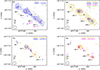Fig. 1.

Overlap of contours corresponding to the velocity integrated species emission, ordered by their upper energy level, E_u. A spatial scale of 50 pc corresponds to ∼3″. The kinematic centre (α_ICRS = 00^h47^m33.14^s and δ_ICRS=−25°17′17.52″; Müller-Sánchez et al. 2010) is labelled by a filled black triangle. The black crosses mark the positions analysed in this work and correspond to GMC 7, GMC 6, pSSC 5 and pSSC 2. For reference, the position of GMC 3 and GMC 4 (Leroy et al. 2015) are indicated by magenta crosses in the panel a. The beam size if depicted in the lower left corner of each box. Contours of CH₃NH₂, CH₃CHO, CH₂NH, NH₂CHO, and C₂H₅OH are in grey, blue, orange, magenta, and green, respectively. a) Contour overlap of CH₃NH₂ (3_−1,1−2_0,0;E_u = 17 K) and CH₃CHO (1_1,5−1_0,5 (E+A); E_u = 19 K). Contours start at 3σ with steps of 3σ with 1σ = 42 and 25 mJy beam⁻¹ km s⁻¹, respectively. b) Contour overlap of CH₂NH (4_1,3−3_1,2;E_u = 39.8 K) with 1σ = 78 mJy beam⁻¹ km s⁻¹, CH₃CHO (9_2,9−8_1,8 (E+A); E_u = 43 K) with 1σ = 55 mJy beam⁻¹ km s⁻¹, NH₂CHO (8_0,8−7_0,7; E_u = 36 K) with 1σ = 58 mJy beam⁻¹ km s⁻¹, and t-C₂H₅OH (6₄−5₃; E_u = 37.7 K) with 1σ = 64 mJy beam⁻¹ km s⁻¹. Contours start at 3σ with steps of 3σ for CH₃CHO and t-C₂H₅OH, 8σ for CH₂NH, and 2σ for NH₂CHO. c) Contours overlap of CH₂NH (6_1,6−5_1,5;E_u = 69.6 K) with 1σ = 42 mJy beam⁻¹ km s⁻¹ and CH₃CHO (11_2,9−10_2,8 (E+A); E_u = 70.5 K) 1σ = 25 mJy beam⁻¹ km s⁻¹. Contours start at 3σ with steps of 5σ and 3σ for CH₂NH and CH₃CHO, respectively. d) Contour overlap of CH₂NH (8_1,7−8_0,8;E_u = 122.7 K), with 1σ = 61 mJy beam⁻¹ km s⁻¹ and NH₂CHO (15_2,14−14_2,13; E_u = 133.5 K) 1σ = 78 mJy beam⁻¹ km s⁻¹. Contours start at 3σ with steps of 2σ.

Finally, the emission of the iCOMs studied in this work is relatively faint towards GMC 5, which lies close to the kinematic centre. Moreover, this region shows particular absorption features due to the strong radio continuum emission (Meier et al. 2015; Humire et al. 2022) and would require a specific radiative transfer modelling, which is beyond the scope of this paper. We thus excluded this GMC from our analysis. As a result, in the rest of the paper, we focus on positions which we named as GMC 7, GMC 6, pSSC 2, and pSSC 5, whose coordinates are listed in Table 1. Below, we describe and compare the emission distribution of the selected species towards these four regions in Sect. 3.1 and we describe the extraction and analysis of the spectral lines in Sect. 3.2.

Table 1.

Selected regions and coordinates.

3.1. Emission distribution

To generate the moment maps, we looked for transitions that were isolated enough (i.e. with either no contribution from other adjacent species or with a contamination from adjacent features that is below 3σ level) within the range of velocity on which we integrate the emission. We then integrated the emission over the full line profile, taking into account the velocity shift across the regions; hence, within the range of [70; 380] km s⁻¹. The transitions used to perform these moment maps are labelled in the spectra of the brightest region, GMC 6, in the figures of Appendix B on Zenodo. The corresponding spectral parameters of the transitions are shown in the same appendix.

Figure 1 shows the integrated line emission distribution of the five iCOMs, grouped in four E_u ranges, to minimize biases due to different excitation conditions. For each E_u range, we superposed the contour maps of the various species to visually show the overlap between their emission distribution. Since we have a limited sample of moment 0 maps for the five iCOMs, we could not always simultaneously compare their emission distribution at each E_u range. Panel a of Figure 1 shows the contour maps of the CH₂NH and CH₃NH₂ transitions close to E_u = 20 K. Panel (b) shows the contour overlap of all species except CH₃NH₂ at E_u = 30−40 K. Panel (c) shows the contour maps of the CH₂NH and CH₃CHO transitions at E_u∼70 K. Finally, panel d shows the contour maps of CH₂NH and NH₂CHO around E_u>100 K.

From Figure 1, we can see a difference in the spatial emission of the iCOMs across the four regions. First, CH₃NH₂ shows more extended emission than CH₃CHO towards the part of the CMZ encompassing the regions GMC 6 to pSSC 2, as seen in Figure 1, panel a. On the other hand, the emission of CH₃CHO dominates towards GMC 7 compared to that of CH₃NH₂. For the transitions with upper energy levels around ∼30−40 K (see Figure 1b), we can see that each GMC seems to show a different chemical composition: the CH₂NH and C₂H₅OH emission dominate GMC 7 and show the most extended emission throughout the regions. However, there is a lack of C₂H₅OH emission towards the kinematic centre (indicated by a black triangle in Figure 1) compared to CH₂NH. On the other hand, the emission of CH₃CHO and NH₂CHO is more compact around the GMCs. Both species show emission towards GMC 6 and have faint emission toward GMC 7, but whilst CH₃CHO emission covers both pSSC 5 and pSSC 2, NH₂CHO lacks emission towards pSSC 2. At E_u∼70 K (see Figure 1c), both CH₂NH and CH₃CHO show emission towards GMC 6 with CH₂NH showing a slightly more spatially extended emission compared to CH₃CHO. On the other hand, only CH₂NH emits towards pSSC 5 and the two species are fainter towards pSSC 2 and GMC 7. For E_u>100 K (see Figure 1d), we see that both CH₂NH and NH₂CHO emit towards GMC 6 and pSSC 2 but CH₂NH shows a more extended emission. CH₂NH only emits towards pSSC 5 and both species are absent at GMC 7. Interestingly, whilst NH₂CHO showed fainter emission for E_u∼30−40 K towards pSSC 2, it shows stronger emission for E_u>100 K. Whilst the emission of the iCOMs seems to show a spatial disparity within the inner GMCs of NGC 253, we should keep in mind that fainter emission could be due to either a true lower abundance or a sensitivity bias if the transition is not very intense (band 5 observations were less sensitive compared to the rest of the data; see Martín et al. 2021). Hence, the investigation of whether there is a disparity among the species across the region comes after we have derived the physical parameters (Sect. 4).

Finally, we can see an evolution in the emission morphology compared to E_u: Looking at CH₃CHO and CH₂NH for which we imaged transitions from 19 K to 70.5 K and from ∼40 K to ∼123 K, respectively, we see the emission being more compact with increasing E_u. This shows that transitions with different E_u may be excited under different conditions and it is important to compare spatial extent of species which have similar upper level energies. All the velocity-integrated maps obtained for each species are shown in Figures A.1–A.5.

3.2. Spectra and line parameters

We extracted the spectra towards GMC 7, GMC 6, pSSC 5, and pSSC 2 from regions of a beam-size (1.6″×1.6″) and centred on the coordinates given in Table 1. We then centred each spectrum at the local standard of rest velocity (LSRK) corresponding to the rest frequency of each transition used in this work before performing a Gaussian line fitting to the detected transitions. A threshold of 3σ on the intensity peak was set to consider a line to be detected. Transitions that had been contaminated by more than 15% by a transition from another species (i.e. contributing to 15% or more of the total integrated intensity of our desired transition) or that were too blended to perform a multiple Gaussian fit were not taken into account. To assess whether a line is contaminated, we used the existing line identification of ALCHEMI 7 m and 12 m data (Martín et al. 2021 and priv. comm.) and performed an additional inspection using WEEDS (Maret et al. 2011). This is an extension of CLASS that uses both the Jet Propulsion Laboratory (JPL; Pickett et al. 1998) and the Cologne Database for Molecular Spectroscopy (CDMS; e.g. Müller et al. 2005; Endres et al. 2016) databases. However, in the case of CH₃CHO, the E- and A- states are often completely blended together and the spectral resolution of 10 km s⁻¹ is insufficient to disentangle the two states. Similarly, for NH₂CHO and CH₃NH₂, there are two transitions with similar spectroscopic parameters are completely blended together. In these cases, we still kept these transitions and performed a single line Gaussian fit. We explain how we used these transitions for the analysis in Sect. 4.1. We present the list of all of the transitions per species and per region used in this work, as well as their spectroscopic parameters, in Appendix B on Zenodo. We detected only the form anti of C₂H₅OH among the different rotamers, but this is not surprising as the form anti is the most stable rotamer (Pearson et al. 2008; Bianchi et al. 2019); thus, C₂H₅OH refers to this form only.

From the Gaussian line fitting procedure, we extracted the integrated intensities (∫T_B.dV) in K km s⁻¹, the line widths (FWHM), and the peak velocity (V_peak), both in km s⁻¹. The extracted spectra, the best Gaussian fits and a summary of the Gaussian line-fitting results and rms for each transition and region are available in Appendix B on Zenodo.

4. Derivation of the physical parameters

4.1. Methodology

For each species and each of the four selected regions, we detected enough transitions (>7 for most species and regions) with a broad enough range of E_u covered to derive the column densities and rotational temperatures using the rotational diagram (RD) method (Goldsmith & Langer 1999). This method assumes local thermodynamic equilibrium (LTE) and optically thin emission. These assumptions are revisited later in this work based on the case of CH₂NH (see Sect. 4.3). We also assumed the Rayleigh-Jeans approximation holds. We included a calibration error of 15% (see Sect. 2) and the spectral rms in the integrated flux uncertainties. The best fit was calculated by minimizing the reduced chi-square, $χ_{r}^{2}$ $\chi _r^2$ .

As a first approximation, we set the beam-filling factor² to 1/2, assuming that our emission comes from the GMC scales (hence from a region of the size of the beam or 1.6″). However, in some regions and for some species, we saw a clear deviation in the rotational diagram for the higher E_u transitions. This behaviour can be either due to the presence of multiple gas components with different physical conditions or to non-LTE (NLTE) or opacity effects (Goldsmith & Langer 1999). We favoured the first option, namely, the presence of multiple gas components. Our choice is supported by the fact that higher upper-energy level transitions showed often a different FWHM or V_peak compared to the lower upper-energy transitions (see discussion in Sect. 4.2 below) and the difference in the emission distribution of the species depending on the excitation conditions (see Sect. 3.1). For these cases, we assumed that the first component, traced by the lower upper-level energy transitions, arises from the GMCs; whilst the second component, traced by the higher upper-level energy transitions, arises from the pSSCs. For the latter component, we calculated the beam-filling factor using a size for the pSSC clusters of 0.12″ (corresponding to ∼2 pc), estimated by Leroy et al. (2018). This assumption is supported by the fact that the emission is more compact with increasing E_u, which sometimes goes unresolved by the ALCHEMI beam (See Figure 1).

Finally, as mentioned in Sect. 3.2, most of the E- and A- states of CH₃CHO and some transitions for NH₂CHO, CH₃NH₂ and C₂H₅OH are too blended to perform a multiple Gaussian fit. As the blended transitions have the same spectroscopic parameters (E_u,A_ij,g_u), thus, we assumed that each transition accounts for 50% of the total line integrated intensity. Furthermore, for CH₃CHO, we assumed a CH₃CHO-E/CH₃CHO-A ratio of 1, since the kinetic temperature is higher than the energy difference of ∼0.1 K between the levels of the different symmetry states (Matthews et al. 1985). Therefore, we included each pair of blended transitions in the RDs by attributing 50% of the total integrated intensity, given in Appendix B on Zenodo, to each individual transition.

4.2. Rotational diagrams

In Figure 2, we show as an example the rotational diagrams obtained for each species towards GMC 6, which is the region showing the most intense emission (see Sect. 3.1). The RDs at other positions are available on Appendix C on Zenodo. In the case of GMC 6, two temperature components were needed for CH₃NH₂, NH₂CHO, and CH₃CHO. Two temperature components were also needed for pSSC 2 (CH₃NH₂ and NH₂CHO) and for pSSC 5 (CH₃NH₂ and CH₃CHO). For CH₃NH₂ and CH₃CHO, the deviation occurs near E_u∼40 K and it is closer to 60 K for NH₂CHO. When two temperature components are present in the RDs, we made the assumption that they are not arising from the same spatial component. The low E_u transitions being more spatially extended compared to the higher E_u transitions (see Sect. 3.1), we assumed that whilst the former mainly arises from GMC scales, the latter arises from more compact scales, such as the pSSC scales (i.e. the structures identified next within the GMCs). As a caveat, this implies that the contribution from the warm compact component to the cold extended one is negligible.

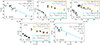Fig. 2.

Rotational diagrams of each species towards GMC 6. Parameters E_u, N_u, and g_u are the level energy (with respect to the ground state), column density, and degeneracy of the upper level, respectively. The error bars on ln(N_u/g_u) include a calibration error of 15% (see Sect. 2). The blue (and orange if a second component is fitted) solid lines represent the best fits and the dashed grey lines are the extrapolations of the fit for the full range of E_u covered. The source size assumed is indicated for each component (see Sect. 4.1).

For the species showing two temperature components, we looked at the Gaussian fit results to check for any shift in the mean FWHM or V_peak as a function of the upper-level energy. In the following, we discuss first about the Gaussian fit results in the context of the two temperature components (Sect. 4.2.1) before discussing the results from the RDs (Sect. 4.2.2).

4.2.1. Gaussian fits and temperature components

To check whether the presence of the two temperature components seen in the RDs for CH₃CHO, CH₃NH₂, and NH₂CHO can be identified through a shift in the mean FWHM or V_peak as a function of the upper-level energy, we used only relatively isolated transitions, where a single Gaussian fit was performed to get the most reliable measurement for FWHM and V_peak. In the case of auto-blended transitions, we kept only those for which the two lines are separated enough to perform two separate Gaussian fits. Figure 3 shows the FWHM and V_peak as a function of E_u towards GMC 6, pSSC 5, and pSSC 2, where a second gas component has been fitted in the RDs. The uncertainties were derived by adding in quadrature the errors from the Gaussian fits with the spectral resolution of 10 km s⁻¹. The mean FWHM and V_peak for each component are summarised in Table B.2 on Zenodo. We discuss the individual species below:

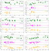Fig. 3.

Line widths (FWHM; left-hand side) and peak velocities (V_peak; right-hand side) as a function of upper level energies (E_u) for CH₃OH (top panels), CH₃NH₂ (middle panels), and NH₂CHO (bottom panels) and for GMC 6 (filled green circles), pSSC 5 (filled magenta pentagons), and pSSC 2 (filled orange diamonds). The vertical dashed grey lines indicate where the deviation in the RDs occurs, i.e. ∼40 K, 30 K, and 60 K for CH₃CHO, CH₃NH₂, and NH₂CHO, respectively. Only the most clear Gaussian fits have been used (see text). If a second component has been identified in the RDs, it is shown in lighter color. Mean FWHM and V_peak are indicated on the plots by horizontal dashed lines accompanied with their corresponding values.

CH₃CHO (Figure 3, top panels): We see a clear difference in the mean V_peak for GMC 6, where we see an increase in the V_peak with increasing E_u. However, we cannot see this shift toward pSSC 5, where a second temperature component has also been fit in the RD (see Appendix C on Zenodo), due to the lack of reliable Gaussian fit measurements.

CH₃NH₂ (Figure 3, middle panels): A slight decrease in the line widths with increasing E_u is seen towards GMC 6 and pSSC 5, although it is quite marginal. No variation in the FWHM is seen towards pSSC 2 and no difference in the V_peak is seen towards any of the regions in CH₃NH₂. Thus, we find no strong indication of two different components for CH₃NH₂ and the deviation in the RD could be due to NLTE effects (Goldsmith & Langer 1999).

NH₂CHO (Figure 3, bottom panels): An increase in V_peak is relatively clear with increasing E_u towards the two regions where two components were fitted (i.e. GMC 6 and pSSC 2). For pSSC 2, we also observe a decrease in the FWHM simultaneously with an increasing E_u, and this can be seen more moderately towards GMC 6. Interestingly, the shift in V_peak and in FWHM seems to occur closer to 40, compared to what is seen in the RDs, which could indicate that the majority of the NH₂CHO emission could be associated with the second higher temperature component.

In conclusion, with the current spectral resolution as a main contributor to the uncertainties, the presence of two components is only clear for NH₂CHO, whilst it is not clear for CH₃CHO and CH₃NH₂. In addition, we should note that optically thick lines can induce larger line widths. Higher spectral and angular resolution observations are needed to identify possible different gas components more clearly.

4.2.2. Results from the rotational diagrams

Figure 4 shows an overview of the derived T_rot and N_tot for each species and region listed in Table C.1 on Zenodo. Due to the fact that we observe deviations from the fits in the RDs, it is clear that the derived T_rot values are not representative of the true gas temperature. For the rotational temperatures (top panel of Figure 4), we do notice some differences between the regions. In particular, GMC 7 shows only a cold (T_rot≤20 K) component compared to the other regions. On the other hand, the other regions have two components, a cold (T_rot≤20 K) and a warmer component (T_rot∼30−80 K). Finally, none of the regions shows a hot (T_rot>100 K) component, which would have been expected if the iCOMs were thought to be emitted from a hot-core-like (T>100 K; see e.g. Kurtz et al. 2000) region. On the other hand, this result is similar to the Milky Way's Galactic Centre (GC), where widespread emission (a few tens to hundreds of parsecs) from iCOMs has been measured (e.g. Requena-Torres et al. 2006; Li et al. 2017, 2020). There, low rotational temperatures (T_rot≤20 K; e.g. Requena-Torres et al. 2006; Zeng et al. 2018; Rivilla et al. 2022b) were also derived, indicating that the GC iCOM emission is sub-thermally excited. The extended iCOM emission toward the GC is not associated with hot cores and can be explained by widespread recurrent low-velocity shocks (Requena-Torres et al. 2006; Zeng et al. 2020).

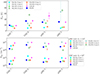Fig. 4.

Derived rotational temperature (T_rot; top) and total column density (N_tot; bottom) for each species and region. The order of the regions follows the layout of the GMCs/SSCs of the CMZ from north-east to south-west as shown in Figure 1. Top: when two gas components were fitted in the RDs, the T_rot of the two components are indicated. Bottom: column densities derived for GMC scales (θ_s = 1.6″; bottom part) and pSSC scales (θ_s = 0.12″; top part). For the species (CH₂NH and C₂H₅OH) and region (GMC 7), where only one gas component was fitted, we calculated the column densities for the two scales. For the other regions and species, we attributed the first component to an emission coming from GMC scales and the second component to an emission coming from pSSC scales. In the cases of NH₂CHO and CH₃CHO, only one component was fitted for pSSC 2 and pSSC 5, respectively.

For the column densities (bottom panel of Figure 4), we describe the behaviour separating the emission from the cold component (derived with θ_s = 1.6″; i.e. GMC scale) and the warm component (derived with θ_s = 0.12″, i.e. pSSC scale) transitions, as given below. Only one temperature component was fitted for all species towards GMC 7, CH₂NH and C₂H₅OH towards all regions, NH₂CHO towards pSSC5, and CH₃CHO towards pSSC2. In these cases, since we did not have knowledge of the region of emission of these species, we calculated the column densities for the two emission sizes, namely: for the GMC scale (θ_s = 1.6″) and pSSC scale (θ_s = 0.12″).

GMC-scales: C₂H₅OH and CH₃CHO show relatively constant column densities throughout the regions. On the other hand, NH₂CHO, CH₃NH₂, and CH₂NH show a decrease in N_tot towards GMC 7 and the column density of CH₃NH₂ increases towards GMC 6. Overall, C₂H₅OH and CH₃NH₂ show the highest column densities, except towards GMC 7 where the column density of CH₃NH₂ decreases.

pSSC-scales: For C₂H₅OH and CH₂NH, the trend in column density is the same as at GMC-scales since the two species have only one component. In the case of CH₃NH₂, its column density is constant across the regions except towards GMC 7, where it decreases. In the cases of NH₂CHO and CH₃CHO, if we consider only the second components (high E_u) towards GMC 6 and pSSC 5 for CH₃CHO and pSSC 2 for NH₂CHO, then the column density of both species is the highest towards GMC 6. If we consider that in the other regions where only one component is detected (low E_u transitions), then the column density of CH₃CHO is the lowest towards pSSC 5 and that of NH₂CHO is the lowest towards GMC 7 and pSSC 2.

We note that since the four regions do not have the same H₂ column densities, the abundance trends could be different than the column density trends. However, an abundance study is beyond the scope of this paper. We simply stress here that there are variations of the relative column densities between the species across the regions, indicating possible chemical differences, for instance, towards GMC 7, where the relative amount between O-bearing and N-bearing iCOMs changes compared to the other regions. We discuss chemical variations in more details in Sect. 5.3.

4.3. NLTE analysis: CH₂NH

CH₂NH is the only species from this work for which collisional excitation rates are available. Therefore, we can perform a NLTE analysis to constrain more accurately the gas physical parameters traced by CH₂NH toward the CMZ of NGC 253.

We performed this analysis using the large velocity gradient (LVG) code grelvg (Ceccarelli et al. 2003). We used the CH₂NH–H₂ collisional rates from Xue et al. (2024) available in the Excitation of Molecules and Atoms for Astrophysics (EMAA) database³. The rates were calculated for a temperature in the range 10–150 K and for the transitions up to E_u = 143 K. Therefore, the maximum temperature tested is limited by the available rate coefficients and the CH₂NH transition at 312.336 GHz with E_u = 151.3 K, which we detected in this work, was excluded from the analysis. For each region we ran a grid of models (∼10 000), varying the column density, the gas density, and temperature within 10¹³−10¹⁸ cm⁻², 10⁴−10⁸ cm⁻³, and 10−150 K, respectively. The column densities and gas densities were both sampled in logarithmic scale and the gas temperature was sampled in linear scale. We left the source size as a free parameter. Then, for the geometry, we chose a uniform sphere (Osterbrock 1974) as the most physically realistic choice. The ortho-to-para ratio of H₂ was set to the statistical value of 3. Finally, the average line widths of CH₂NH chosen is 50 km s⁻¹, which is the average line width across the regions (see Table B.2 on Zenodo). We also included a 15% calibration uncertainty in the integrated intensity (see Sect. 2).

From the RD analysis, there is no clear indication of a multiple temperature components for CH₂NH (see e.g. Figure 2). We thus first included all the lines in the LVG code. However, this resulted in a bad fit ( $χ_{r}^{2} > 5$ $\chi ^2_r>5$ ) for GMC 6, pSSC 5, and pSSC 2. In these regions, the two transitions of CH₂NH at 225.554 and 172.267 GHz are not well fit with the other transitions. These lines have the lowest E_u (<20 K) and could thus be coming from a cooler or more extended component compared to what the other transitions (E_u = 27−151 K) trace. Since we cannot perform the LVG analysis with only two lines, we cannot constrain the physical parameter of this potentially cooler component. We thus ran the LVG with the rest of the lines (E_u≥27 K).

Figure 5 shows the results of the LVG analysis for each of the four regions. The best fit for the CH₂NH column densities is similar towards the four regions with values in the range (1.5−2)×10¹⁶ cm⁻². The kinetic temperatures are not always well constrained and are limited by the maximum temperature available from the collisional rates (150 K). We thus have an overall lower limit of T_kin≥(20−50) K across the different regions. For the derived gas densities, they lie mostly between n(H₂) = (10⁵−10⁶) cm⁻³ except for GMC 7, where n(H₂)≤10⁵ cm⁻³. In all the regions, several lines were found to be optically thick with τ>1 (see Table 2). Finally, the best fit for the emission size is in the range 0.19″−0.26″ corresponding to a linear scale of ∼3−4 pc in diameter. The best-fit solutions and ranges obtained for each source are reported in Table 2. The 1σ confidence levels constrained correspond to a 68% confidence range.

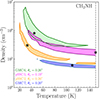Fig. 5.

Volume density and kinetic temperature contour plots showing the results from the LVG analysis for CH₂NH towards GMC 7 (blue), GMC 6 (green), pSSC 5 (magenta), and pSSC 2 (orange). The contours show the 1σ solutions obtained for the minimum $χ_{r}^{2}$ $\chi ^2_r$ value in the column density parameter. The best fits are marked by black stars, while the best fit for the emission size (θ_s) are indicated in the bottom-left corner of the figure. The vertical grey line indicates the maximum temperature at which the rates are calculated.

Table 2.

Best fit results and 1σ confidence level range from the NLTE LVG analysis of CH₂NH.

We corrected the rotational diagram for the optical depth and source size for all the regions using the population diagram method (Goldsmith & Langer 1999), taking the output values of the LVG analysis for these parameters to investigate whether the optical depth effects are dominant. For consistency, we removed the transitions that were left out from the LVG analysis (see above). The corrected RDs are shown in the Appendix C on Zenodo. We still found some deviation from a straight line in the corrected RDs, with rotational temperatures below the minimum gas temperature predicted by the LVG analysis. Therefore, we find that CH₂NH is also affected by NLTE effects. This result is consistent with that of Faure et al. (2018), who found that NLTE effects can be expected in the density range of $n_{H_{2}} = 10^{3} - 10^{7}$ $n_{{\textrm {H}}_2} = 10^3{-}10^7$ cm⁻³ for this species. We do note, however, that in the discussion below, we use the column densities derived with the RDs for CH₂NH, since the goal of performing population diagrams was only to evaluate the contribution of NLTE effects.

5. Discussion

As mentioned in the introduction, investigating iCOMs in more extreme star formation conditions than those found in our own Galaxy allows us to probe the universality (or otherwise) of our chemical diagnostics and whether they remain valid in extragalactic environments. Below, we qualitatively discuss whether the known proposed formation pathways for iCOMs could also be valid in NGC 253 and whether the iCOMs in this study can be chemically linked (Sect. 5.1). We then discuss their possible region of emission and the physical processes they might be tracing (Sect. 5.2). Finally, we focus on the small chemical differences within the regions (Sect. 5.3). Figure 7 shows a schematic summarising our main hypotheses and scenarios concerning iCOMs towards the CMZ of NGC 253, focussing in particular on the discussion from Sects. 5.1 and 5.2.

5.1. Chemical link and formation pathways for iCOMs

Understanding which chemical pathways to the formation of a specific species are dominant within an environment is not straightforward. From observations, a method that is regularly used is to look at the abundance correlations between two species suspected to be chemically linked or to have a similar precursor (e.g. Yamamoto 2017; Coletta et al. 2020; Li et al. 2024). However, it is worth noting that a correlation between two species does not always imply a direct chemical link. It may also indicate that they went through similar physical processes of formation across different environments (e.g. Quénard et al. 2018; Belloche et al. 2020).

Figure 6 shows the relation between the column densities of the iCOMs, at both GMC scales (corresponding to a source size of 1.6″) or pSSC scales (corresponding to a source size of 0.12″). We list below several trends from Figure 6 that will be discussed below. We refer to CH₃CHO and C₂H₅OH as O-bearing iCOMs, and then CH₂NH and CH₃NH₂ as N-bearing iCOMs, while NH₂CHO lies in between the two categories.

At GMC scales, O-bearing species are well correlated over the four regions and present a constant ratio [C₂H₅OH/CH₃CHO] of 3 (panel a). The correlation disappears at pSSC scales (panel f).
At both GMC- and pSSC scales, there is an enhancement in O-bearing species compared to N-bearing species (including NH₂CHO) towards GMC 7 (panels b, c, h, and k).
At GMC scales, CH₃NH₂ and NH₂CHO are relatively well correlated over the four regions and present a constant ratio [CH₃NH₂/NH₂CHO] of ∼3 (panel d). At pSSC scales, the ratio increases towards GMC 7 and pSSC 2 (panel i).
The ratio [CH₃CHO]/[NH₂CHO] varies greatly from GMC scales (panel b) to pSSC scales (panel g).
The abundance ratio between CH₃NH₂ and CH₂NH (panels e, j) is close to 3 at both scales, but slightly lower for GMC 6 at pSSC scales.

In the following sub-sections, we look for correlations between the derived column densities of a few pairs of iCOMs, which are thought to share chemical roots. We first recall the known formation pathways of the different species before discussing whether a certain formation pathway is most probable for the CMZ of NGC 253, as well as whether a chemical link between the pairs of species discussed is possible. A summary of plausible formation pathways for each iCOM is shown in Figure 7.

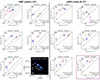Fig. 6.

Relation between the column densities of the iCOMs derived from the rotational diagrams at GMC scales (θ = 1.6″; left-hand side of the figure) and at pSSC scales (θ = 0.12″; right-hand side of the figure), for each region (GMC 7: blue; GMC 6: green; pSSC 5: magenta; pSSC 2: orange). Pearson's coefficient and p-values are indicated in the bottom right part of each plot. Dashed and full grey lines indicate abundance ratio factors. Panel k is highlighted as the correlation between CH₂NH and C₂H₅OH is the same at both GMC-scale and pSSC-scale. For reference for the location of each region, we added a map of the CH₂NH (4_1,3−3_1,2) transition in the bottom-left part of the figure.

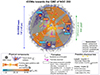Fig. 7.

Schematic (not to scale) of summarising the possible formation pathways and chemical links between the iCOMs (Sect. 5.1) and their emission origins (Sect. 5.2) within a GMC. The temperatures reported are averaged over the region but there can be variation from one region to another. We assume the size of a GMC is comparable or larger than the size of the ALCHEMI beam of 1.6″ (or ∼27 pc). Formation and chemical links: Sputtering from the ice grain mantle and gas phase formation pathways are both possible to explain the iCOM emission at GMC scales, whilst at SSC scales, the dust temperature can be high enough to allow thermal desorption. CH₃CHO and C₂H₅OH can also be chemically linked (i) both on the grain (with CH₃CHO as the precursor of C₂H₅OH) or via the Ethanol tree in the gas phase (with C₂H₅OH as a precursor for CH₃CHO). CH₃NH₂ and CH₂NH could be chemically linked (ii) by sharing similar precursors, both on the grain or in the gas phase (if the gas temperature is higher than 100 K; e.g. Halfen et al. 2013). Origin: At the scale of GMCs, the iCOMs are likely tracing large-scale shocks, due to either cloud-cloud collision (1) or shocks related to star formation activity (scenario 2a; see also Huang et al. 2023). At pSSC scales, iCOMs could trace either star formation-related heating process (scenario 2b; CH₃NH₂, NH₂CHO) and shocks (scenario 2a; CH₃CHO, CH₂NH, C₂H₅OH), associated or not (i.e. if cloud-cloud collision, scenario 1) with star formation.

5.1.1. CH₃CHO and C₂H₅OH

The formation pathways of CH₃CHO are debated. Both gas-phase and grain-surface reactions are proposed. Among the viable gas-phase formation pathways, CH₃CHO could be formed either from the radical C₂H₅ previously formed on the grain and ejected in the gas phase (e.g. Charnley 2004; Vasyunin & Herbst 2013; Barger & Garrod 2020; Codella et al. 2020; De Simone et al. 2020; Vazart et al. 2020) or from C₂H₅OH (known as the ‘ethanol tree’; e.g. Skouteris et al. 2018; Vazart et al. 2020). However, whilst the first pathway has been validated in both cold and warm environments, the validity of the second one has not been checked in cold environments (e.g. Vazart et al. 2020). Alternatively, various grain-surface reactions have been proposed for the formation of CH₃CHO (e.g. Bennett et al. 2005; Garrod et al. 2008; Ruaud et al. 2015; Lamberts et al. 2019; Barger & Garrod 2020; Martín-Doménech et al. 2020; Ibrahim et al. 2022), although the efficiency of some of these reactions has been debated (e.g. Rimola et al. 2018; Enrique-Romero et al. 2016, 2021). For C₂H₅OH, grain-surface reactions are mostly proposed but there is no consensus on the formation process (e.g. Jin & Garrod 2020; Chuang et al. 2020; Perrero et al. 2022; Enrique-Romero et al. 2022; Garrod et al. 2022; Molpeceres et al. 2024a). One of the proposed pathways involves CH₃CHO as a precursor (Bisschop et al. 2007; Chuang et al. 2020; Fedoseev et al. 2022), where it was expected that the solid-state abundances of C₂H₅OH would be lower than those of CH₃CHO (Sivaramakrishnan et al. 2009; Fedoseev et al. 2022). This formation pathway could be ruled out since recent observations made with the James Webb Space Telescope showed relatively similar ice abundances for the two species (Rocha et al. 2024; Chen et al. 2024), as found previously in the case of comets (Rubin et al. 2019). However, a direct comparison of the content seen in the ice and in the gas towards two low-mass protostars showed that this is not what is seen in the gas phase, where C₂H₅OH seems to be more abundant than CH₃CHO (Chen et al. 2024). On the other hand, gas phase reactions starting from H₃O⁺+C₂H₄ and leading to the formation of C₂H₅OH through C₂H₅OH₂⁺ as a precursor have been reported in both the KIDA⁴ and UMIST⁵ databases; thus, this could be a viable pathway if H₃O⁺ is abundant enough (which may be the case due to the high CRIR towards these regions; e.g. Holdship et al. 2022; Behrens et al. 2024). In the following, we investigate whether ethanol (C₂H₅OH) and acetaldehyde (CH₃CHO) are correlated towards NGC 253.

Table B.2 on Zenodo shows that the mean FWHM and peak velocities of C₂H₅OH are generally more consistent with that of the colder component of CH₃CHO. Optical depth effects could alter these results but further similarities can be seen when looking at the column densities of the two species: From Figure 4, we see that both the column densities derived for GMC scales of C₂H₅OH and CH₃CHO are relatively constant throughout the four regions. In addition, their abundance ratio of ∼2.3 is also constant across the regions and show the best correlation at GMC scales (see Figure 6a). Therefore, a correlation between the cold component of CH₃CHO (governed by the low E_u transitions) and C₂H₅OH could indicate that the two species are chemically linked (see Fig. 7, hypothesis i). Since the abundance of C₂H₅OH is higher than that of CH₃CHO, the two species could be linked via the gas-phase production of CH₃CHO through the ethanol tree. This hypothesis, if true, implies that the ethanol tree pathway proposed by Skouteris et al. (2018) would also be valid at low temperatures, since the iCOMs are likely sub-thermally excited. On the other hand, we cannot rule out that the two species were formed on the grains before being ejected through shocked processes (see Sect. 5.2). The higher abundance of C₂H₅OH compared to that of CH₃CHO could then indicate more fast or important destruction or reprocessing of CH₃CHO in the gas phase compared to C₂H₅OH. For C₂H₅OH, one proposed formation path for its precursor C₂H₅OH₂⁺ is via the gas phase reaction between H₃O⁺ and C₂H₄. Considering the high CRIR derived towards NGC 253 (e.g. Holdship et al. 2022; Behrens et al. 2022), the abundance of H₃O₊ could be high enough for the gas phase production of ethanol to be viable.

When looking at the correlations at pSSC scales (see Figure 6f), the warm component of CH₃CHO (traced by the high E_u transitions) towards GMC 6 and pSSC 5 is no longer correlated with ethanol. The difference in peak velocity and FWHM for this high E_u transitions, compared to the low E_u transitions (see Table B.2 on Zenodo) indicates that additional CH₃CHO is produced in these two regions and likely through a different pathway. If the cold component of CH₃OH is formed in the gas phase, the warm CH₃CHO component could, on the other hand, form on the icy grain mantles via thermal desorption (if the gas temperature is high enough; see Sect. 5.2.2); alternatively, it could form via non-thermal processes such as shocks (e.g. Ruaud et al. 2015; Lu et al. 2025). We investigate the origin of the high excitation of CH₃CHO in GMC 6 and pSSC 5 in Sect. 5.3.

5.1.2. NH₂CHO

Both grain-surface formation (e.g. Raunier et al. 2004; Garrod et al. 2008; López-Sepulcre et al. 2015; Fedoseev et al. 2016; Rimola et al. 2018; Dulieu et al. 2019; Martín-Doménech et al. 2020; Chuang et al. 2022) and gas-phase formation (e.g. Kahane et al. 2013; Barone et al. 2015; Vazart et al. 2016; Skouteris et al. 2017) pathways have been suggested for formamide (NH₂CHO), but which is the most efficient is highly debated, as in the case of CH₃CHO. We refer to López-Sepulcre et al. (2019) and López-Sepulcre et al. (2024) for a comprehensive review of the different formation paths proposed for formamide. Here, we only investigate the potential chemical link of NH₂CHO with HNCO and H₂CO, with both species thought to be chemically linked with NH₂CHO, either as a parent species on the ice grain mantle or in the gas phase (H₂CO; e.g. Fedoseev et al. 2016; Dulieu et al. 2019; Kahane et al. 2013; Vazart et al. 2016; Aikawa et al. 2020; López-Sepulcre et al. 2024) or as a daughter species (HNCO; Brucato et al. 2006; Gorai et al. 2020; Haupa et al. 2022; Chuang et al. 2022). Both H₂CO and HNCO were studied towards the CMZ of NGC 253 (Mangum et al. 2019; Huang et al. 2023, 2025).

Furthermore, HNCO traces low-velocity shocks throughout the CMZ of NGC 253 and the gas temperatures towards the four regions investigated in the present study range between ∼20 and 100 K (Huang et al. 2023). The rotational temperatures we derived range between ∼10−30 K and ∼50−80 K for the cold and warm component, respectively, consistent with that of HNCO. A word of caution is needed, however, since our rotational temperature could be underestimated if optical depth effects or NLTE effects are at play, as we found to be the case for CH₂NH (see Sect. 4.3). Using transitions with similar energy levels, we compared the emission distribution between NH₂CHO and HNCO around ∼40 and ∼140 K as shown in Appendix D (on Zenodo). NH₂CHO is much less intense compared to HNCO, as it is much less abundant, but the two species do not peak towards the same regions. This is also seen when comparing the derived column densities of NH₂CHO and HNCO: whilst HNCO has a relatively constant column density across the regions (Huang et al. 2023), the cold component of NH₂CHO decreases towards GMC 7, whilst the warm component is lower towards pSSC 2. Neither of the two component of NH₂CHO seem thus to be chemically linked with HNCO.

As for HNCO, we also compared the emission distribution of NH₂CHO and H₂CO at similar energy levels, around 45 and 100 K, as shown in Appendix D (on Zenodo). Even though NH₂CHO is much less intense than H₂CO due to its lower abundance, we can see a good correlation between the two species at low E_u with a peak of emission towards GMC 6 and pSSC 5. Therefore, the cold component of NH₂CHO and H₂CO could be chemically linked: H₂CO being likely a gas phase product (Huang et al. 2025), NH₂CHO would thus form in the gas phase, from the reaction H₂CO + NH₂ (Kahane et al. 2013; Barone et al. 2015; Vazart et al. 2016; López-Sepulcre et al. 2024). However, this scenario is challenged by the different temperatures traced by the two species since the rotational temperature for the cold component of NH₂CHO is less than 30 K, while H₂CO was found to trace a warmer gas (T_kin≥70 K at scales 1.6–5″ scales and T_kin≥300 K at scales ≤1″; Mangum et al. 2019; Huang et al. 2025). The low temperature of NH₂CHO could result from sub-thermal excitation. Unless the T_rot values are underestimated, we cannot conclude whether NH₂CHO and H₂CO are chemically linked and whether the cold component of NH₂CHO is a gas-phase or a grain-surface product.

On the other hand, the difference of peak velocities and FWHM for the low and high E_u transitions (see Figure 3) could indicate that NH₂CHO truly traces two different gas components. Indeed, this warmer (T_rot>50 K) component, clearly present in GMC 6 and pSSC 2, shows a narrower mean FWHM, compared to the cold gas component and warmer rotational temperatures (see Figure 4). Hence, another formation pathway could be involved for the warm component of NH₂CHO, different from that of the cold component. As for CH₃CHO, we further investigate the origin of this emission in Sect. 5.3.

5.1.3. CH₂NH and CH₃NH₂

From the literature, CH₃NH₂ is proposed to form on the ice grain surfaces through radical-radical reactions (e.g. Garrod et al. 2008; Kim & Kaiser 2011; Förstel et al. 2017; Enrique-Romero et al. 2022) or from the successive hydrogenation of CH₂NH (e.g. Woon 2002; Theule et al. 2011; Sil et al. 2018; de Jesus et al. 2021; Molpeceres et al. 2024b). Whilst the first pathways overpredicts CH₃NH₂ abundances (Garrod et al. 2008), the second possible pathway has been supported by chemical models reproducing observed abundances of CH₃NH₂ towards high-mass protostars (Suzuki et al. 2016, 2023). This second pathway would indicate that CH₂NH is a precursor of CH₃NH₂ and would also form on the ice grain mantles. However, studies have shown that the conversion of CH₂NH to CH₃NH₂ would be too fast to account for the gas phase abundance of CH₂NH (e.g. Theule et al. 2011; Suzuki et al. 2016). In addition, Molpeceres et al. (2024b) very recently proposed a grain-surface formation route for CH₃NH₂ from the CNH₃ chemisorbate, without passing through CH₂NH as an intermediate species. From the recent literature, it does seem that the two species are not necessarily chemically linked (as had been previously assumed). Alternatively from the grain-surface production, the neutral–neutral gas phase reaction CH₃ + NH₃ → CH₃NH₂ + H has also been proposed as a viable formation pathway in warm (T>100 K) regions (Bocherel et al. 1996; Halfen et al. 2013). Similarly for CH₂NH, various gas-phase formation pathways (ion-molecules or neutral-neutral reactions involving CH₃ or NH₃; see e.g. Table 11 of Suzuki et al. 2016) have been proposed as a viable alternative for the formation of CH₂NH (e.g. Bocherel et al. 1996; Turner et al. 1999; Suzuki et al. 2016; Sil et al. 2018).

From Table B.2 (see Zenodo), both the peak velocities and FHWM of CH₂NH and CH₃NH₂ are consistent with each other (and considering the spectral resolution of 10 km s⁻¹) in all the four regions investigated. From the RDs, we found similar rotational temperatures between CH₂NH and the warm component of CH₃NH₂ in all the regions – except GMC 6 (see Figure 4); however, it was shown that temperatures were underestimated in the case of CH₂NH. For the column densities, since CH₂NH was found to emit at smaller scales than GMC scales (see Sect. 4.3), we compared the column densities of CH₂NH and of the warm component of CH₃NH₂ at pSSC scales only. From Figure 4, the column densities of the warm component of CH₃NH₂ and of CH₂NH are relatively constant across the regions, as seen also in their abundance ratio: Figure 6 shows a very good correlation (panel e) between CH₂NH and the cold component of CH₃NH₂, whilst the correlation becomes weaker (high p-value, panel j) correlation between CH₂NH and the warm component of CH₃NH₂. This weak correlation might be due to the slight decrease in the abundance ratio towards GMC 6, which seems to come from a higher column density in CH₂NH. However, the LVG results did not confirm this increase in CH₂NH towards GMC 6 and the correlation between the two species could be strong for both components of CH₃NH₂.

If the correlation between CH₂NH and CH₃NH₂ is true, the two species could be chemically linked (see Fig. 7, hypothesis ii). Since the grain formation pathways linking CH₃NH₂ and CH₂NH are not viable to explain gas-phase abundance of CH₂NH (see above), the two species can be chemically linked if they share the same precursor. On the grain, the new proposed formation route of the two species from CNH₃ indicates that both species can have HCN and HNC as precursors, without CH₂NH being a precursor of CH₃NH₂. In the gas phase, formation pathways involving CH₃ and NH₃ are viable for both species but only for temperatures above 100 K. Hence, should the two species be chemically linked, both grain-surface and gas-phase reactions could account for the correlation and the chemical link. Our current results, however, do not allow us to distinguish between the two possibilities. Alternatively, the correlation could indicate that the two species trace similar physical processes of formation across the various regions (e.g. Quénard et al. 2018; Belloche et al. 2020).

5.2. Possible origins of the iCOMs in the CMZ of NGC 253

In the previous section, we discussed the iCOMs possible formation pathways and whether any pair of iCOMs has a chemical link. We discuss below the physical process that could be responsible for the iCOMs emission towards the CMZ of NGC 253.

A first inspection of the emission distribution of the iCOMs in this study shows that the emission is (1) mostly concentrated towards the inner part of the CMZ, within 6″ around the kinematic centre, (2) compact around each GMC, and (3) sometimes unresolved for the higher upper-level energies, depending the species. From the images, we thus hypothesize that the emission could be emitted on GMC scales (of the size of the order of the ALCHEMI beam size or 1.6″) and unresolved pSSC scales (∼0.12″ or a few parsecs), which are the next biggest sub-structures identified within the GMCs (e.g. Ando et al. 2017; Leroy et al. 2018). As we could not derive the emission size of the iCOMs (except for CH₂NH) we discuss how they would be produced at GMC and pSSC scales (Sects. 5.2.1 and 5.2.2, respectively) in the following.

5.2.1. iCOMs production at GMC-scales

Several studies derived the volume density and kinetic temperature of the molecular gas in the disk of NGC 253, and found at least two components (e.g. Rosenberg et al. 2014; Gorski et al. 2017; Pérez-Beaupuits et al. 2018; Mangum et al. 2019; Tanaka et al. 2024). The most recent study by Tanaka et al. (2024) derived a gas temperature and density for the low-density component (dominated by the low-J lines of CO and its isotopologues) of 85 K and 2×10³ cm⁻³, respectively, and for the high-density component (dominated by high-density tracers with E_u≤70 K) of 110 K and ∼3×10⁴ cm⁻³, respectively. Their results are consistent with previous studies. The dust temperatures were also estimated to be around 35–40 K (Leroy et al. 2015; Martín et al. 2021). Leroy et al. (2015) derived line widths for the GMCs of NGC 253 of ∼20−40 km s⁻¹ using observations of bulk gas tracers (e.g. low-J lines of CO, HCN, HCO⁺, and isotopologues).

On average, the derived rotational temperatures (T_rot≤60 K) for the iCOMs are thus below the gas temperatures found at GMC scales. At the densities measured (i.e. $n_{H_{2}} \sim 10^{3} - 10^{4}$ $n_{\mathrm {{H_2}}}\sim 10^3{-}10^4$ cm⁻³), the dust and gas are likely not coupled. Most recent laboratory experiments and quantum chemical calculations of binding energies showed that CH₃CHO and CH₃NH₂ would desorb at a lower dust temperature than water (∼100−120 K; Chaabouni et al. 2018; Ferrero et al. 2022; Molpeceres et al. 2022), whilst C₂H₅OH would co-desorb with water at around 140 K (Perrero et al. 2024). On the other hand, NH₂CHO is refractory to water desorption and would desorb at higher dust temperatures (≥170−300 K; e.g. Urso et al. 2017; Chaabouni et al. 2018; Ligterink et al. 2018; Martín-Doménech et al. 2020; Ferrero et al. 2020; Chuang et al. 2022). Therefore, the dust temperature derived at GMC scales (35−40 K) is too low to desorb the iCOMs, if they formed on the icy grain mantles. The iCOMs are very likely sub-thermally excited and are released into the gas phase via non-thermal processes if they formed on the grains. With the CRIR being relatively high (ζ∼10⁻¹⁴−10⁻¹² s⁻¹; e.g. Holdship et al. 2022; Behrens et al. 2022, 2024) towards the CMZ of NGC 253, CR-induced grain heating and sputtering desorption mechanisms (e.g. Roberts et al. 2007; Dartois et al. 2019; Paulive et al. 2022; Arslan et al. 2023) could be an important process in desorbing these iCOMs.

Another important non-thermal process in NGC 253 working to release the species from the ice grain mantles into the gas phase could be shock sputtering. In this work, we measured average line widths of mostly around 40−60 km s⁻¹ (see Table B.2 on Zenodo) for the cold gas component (component 1) of the iCOMs. These values are on average larger than the line widths derived by Leroy et al. (2015) for the GMCs (between 20 and 40 K), which could indicate that the species trace a more turbulent gas. However, as mentioned earlier in this paper, we cannot exclude possible optical depth effects, as is the case for CH₂NH. If we considered moderate to high optical depth (τ∼0.6−3) as we found for CH₂NH, we could end up overestimating the line widths between 12% and 30%⁶. In the most optically thick case derived (τ = 3), for a FWHM of 60 km s⁻¹, the opacity-corrected line width would still be above that of GMCs; however, this would not be the case for a FWHM of 40 km s⁻¹.

O-bearing iCOMs: From Sect. 5.1.1, we found that CH₃CHO and C₂H₅OH could be chemically linked. If this is the case, then the cold component of CH₃CHO could be produced in the gas phase from C₂H₅OH, which would have been sputtered from the grain through shocks. Alternatively, both species could be formed on the grain and be linked with CH₃CHO as a precursor of C₂H₅OH (e.g. Chuang et al. 2020; Fedoseev et al. 2022), but the gas phase abundance ratio would not be representative of the ice abundances (see Sect. 5.1.1). In any case, CH₃CHO and C₂H₅OH tracing shocks would be consistent with the fact that both species are detected in protostellar shocks in our Galaxy (e.g. Arce et al. 2008; Lefloch et al. 2017; Holdship et al. 2019; Csengeri et al. 2019; Codella et al. 2020; De Simone et al. 2020; Busch et al. 2024).

N-bearing iCOMs, including NH₂CHO: Since NH₂CHO has not been detected in cold clouds (López-Sepulcre et al. 2019) and the rotational temperatures for the cold component are low (<30 K) enough to point to sub-thermal excitation, the cold component of NH₂CHO is also very likely to be tracing shocked gas. This would be consistent with what is seen and modelled in Galactic shocked regions (e.g. Arce et al. 2008; Burkhardt et al. 2019; Codella et al. 2017; López-Sepulcre et al. 2024). The correlation of CH₃NH₂ with NH₂CHO at GMC scales (see Figure 6d) could indicate similar physical conditions across these regions for the formation environment of the two species (e.g. Quénard et al. 2018; Belloche et al. 2020), since no chemical reaction linking the two species has been reported in the literature. On the other hand, we found that CH₃NH₂ and CH₂NH could be chemically linked or could trace the same physical process (see Sect. 5.1.3). Therefore, CH₃NH₂ and CH₂NH are also very likely tracing shocked gas. Recently, Zeng et al. (2018) found abundant N-bearing species towards G+0.693-0.027, a molecular cloud in the GC. They mentioned that the rich chemistry of this source is due to the fact that it is dominated by low-velocity shocks and the high cosmic-ray ionisation rates (Rivilla et al. 2022a; Sanz-Novo et al. 2024). They reported a ratio [CH₃NH₂]/[NH₂CHO] and [CH₃NH₂]/[CH₂NH] of 5, which is of the same order of magnitude as our value of ∼3 for both ratios.

Overall, at GMC scales, sputtering due to large-scale shocks is likely the main process releasing the iCOMs into the gas phase. Signatures of shocks have been previously found within the CMZ of NGC 253 were already found in previous studies towards NGC 253 (e.g. García-Burillo et al. 2000; Meier et al. 2015; Haasler et al. 2022; Harada et al. 2022; Huang et al. 2023). Large-scale shocks traced by iCOMs would also be consistent with the origin of CH₃OH, the simplest iCOM, which is also tracing shocks within NGC 253 (e.g. Humire et al. 2022; Huang et al. 2025). We compared the emission distribution of CH₃OH with that of CH₃CHO and CH₃NH₂ around E_u = 20 K and found a relatively good correlation – except towards GMC 7, where we retrieved the O- vs N- disparity. The contour maps of the above-mentioned transitions are shown in Appendix D (Zenodo). Following the possible shock scenarios by Huang et al. (2023), as seen in their Figure 12 in particular, the shocks traced by the iCOMs could be due to either star-formation within each GMC (via shocks induced by outflows or sporadic shocks due to scattered star-formation episodes; see scenario 2a in Figure 7) or cloud-cloud collisions (see scenario 1 in Figure 7).

The intersection of different orbits (such as Lindblad resonances; Iodice et al. 2014) can lead to large-scale cloud–cloud collisions (see Harada et al. 2022; Humire et al. 2022 and references therein). However, the regions we observe are not located close to such intersections, which indicates that the large-scale shocks traced by the iCOMs are either due to cloud-cloud collisions occurring within the GMCs (scenario 1 in Figure 7) or to star formation activity (scenario 2a in Figure 7). From the LVG analysis, we found that CH₂NH is emitted on size scales between 0.15″ and 0.6″, which corresponds to 2.5–10 pc in linear scales, supporting the large-scale shocks scenario within GMCs. The situation could resemble that of our Galactic centre, where the widespread emission of iCOMs is detected throughout the CMZ and are likely caused by low-velocity shocks due to cloud-cloud collisions (e.g. Requena-Torres et al. 2006; Jones et al. 2011; Li et al. 2017, 2020; Zeng et al. 2020). Therefore, chemical modelling will help disentangle between the different shock scenarios. Finally, both O- and N-bearing iCOMs are well correlated – except towards GMC 7, where O-bearing species are more abundant than N-bearing species. We discuss this further in Sect. 5.3.1.

5.2.2. iCOMs production at pSSC-scale

The previously derived temperatures of the pSSCs are ≥100 K (Rico-Villas et al. 2020; Krieger et al. 2020). The PSSCs show clear outflow features (Gorski et al. 2019; Levy et al. 2021), and some of them host super-hot cores (SHCs; Rico-Villas et al. 2020) from the detection of vibrationally excited HC₃N emission and densities and temperatures of ∼10⁶ cm⁻³ and ∼200−300 K, respectively. Such high temperatures are consistent with the kinetic temperatures derived at scales ≤1″ (≤17 pc) using H₂CO observations (Mangum et al. 2019). The densities of the pSSCs are high enough to consider that the dust and gas are coupled. Therefore, the gas temperature at pSSC scales would be enough to thermally desorb the iCOMs (Scenario 2b in Figure 7), should they be formed on grains. Sputtering from shocks due to outflows driven by the stars undergoing formation is also a possible mechanism behind the release of iCOMs into the gas phase or, alternatively, this could lead to a rich gas-phase chemistry, enabling the formation of iCOMs (Scenario 2a in Figure 7).

As for the GMC scales, the rotational temperatures derived for the iCOMs are much lower (T_rot≤60 K) than the gas temperature we expect at pSSCs scales, which could indicate that they are tracing a less dense gas. Therefore, we can see that the iCOMs are very likely sub-thermally excited on pSSC scales as well. Due to the limited temperature range for which the collisional rates were calculated, we could not constrain the upper limit of the gas kinetic temperature – except for GMC 6, where the range is T_rot = 25−130 K (see Sect. 4.3). Suzuki et al. (2016) estimated an upper limit for the desorption temperature of CH₂NH of 160 K, consistent with the mean binding energy of 5534 K derived by Ruaud et al. (2015). If all the iCOMs are tracing the same gas component, then C₂H₅OH and NH₂CHO in GMC 6 cannot be thermally desorbed if they formed on the grain. However, higher temperatures derived in the other regions could indicate that thermal desorption is indeed at work.

O-bearing iCOMs: Both CH₃CHO and C₂H₅OH have been detected in shocked regions associated with outflows from protostars (e.g. Arce et al. 2008; Lefloch et al. 2017), as well as the warm envelope of protostars (e.g. Belloche et al. 2013; Fuente et al. 2014; Jørgensen et al. 2018; Bonfand et al. 2019; Lee et al. 2019; Gorai et al. 2024; Möller et al. 2025). The abundance ratio [C₂H₅OH]/[CH₃CHO] ranging between ∼2.3−5 (see Figure 6f) corresponds well to the abundance ratio found in low- and high-mass star-forming regions, as well as to shocks linked to protostellar outflows (e.g. Lefloch et al. 2017; Chen et al. 2023; Busch et al. 2024).

N-bearing iCOMs, including NH₂CHO: The measured abundance ratio of [CH₃NH₂]/[NH₂CHO] = 3−10 towards GMC 7 and pSSC 5 (see Figure 6i) is similar to the ratios measured in high-mass protostars (Bøgelund et al. 2019b; Nazari et al. 2022). The highest ratios derived towards GMC 6 and pSSC 2 (5 and 10, respectively) are in line with the range of values predicted by the chemical models of hot cores by Garrod et al. (2022) (see their Table 19). The increase in the abundance ratio is due to the smaller column density of NH₂CHO in these regions (see Figure 4). We investigate possible physical causes in Sect. 5.3 below. Finally, the abundance ratio between the warm component of CH₃NH₂ and CH₂NH is close to 3 in all four regions (see Figure 6j), which falls on the lower side of ratios measured in massive protostars (Bøgelund et al. 2019b and references therein, Suzuki et al. 2023). When comparing to the hot core models by Garrod et al. (2022), our measured ratios are well below those predicted by the model (see their Table 17). The discrepancy could arise from the lack of destruction routes of CH₃NH₂ in the model (Garrod et al. 2022). To the best of our knowledge, between the two species, only CH₂NH has been detected in shocked or outflowing regions (e.g. Widicus Weaver et al. 2017; Gorski et al. 2023). From the PCA analysis performed by Harada et al. (2024), CH₂NH was correlated with both shock tracers (SiO) and high-energy transitions of HC₃N, thought to be linked with young starbursts. The warm compact component of CH₃NH₂ could not probe the same gas component as CH₂NH, which can be partially supported by the weak correlation between the two species (see Figure 6).

Overall, if iCOMs are emitted on pSSC scales, the gas could be warm enough to desorb those forming on the icy grain mantles (scenario 2b in Fig. 7). Alternatively iCOMs could be tracing shocks, associated (scenario 2a in Fig. 7) or not (scenario 1 in Fig. 7) with ongoing star formation. With our current angular resolution, we cannot really distinguish between the different scenarios. Higher angular resolution observations and chemical modelling will be necessary to distinguish between the various processes.

5.3. Chemical variations across regions

In the sections above, we found some chemical differences between the four regions. On the one hand, we found that GMC 7 presents an enhancement in O-bearing species compared to N-bearing species. On the other hand, we found that whilst high E_u transitions of CH₃CHO are excited only towards GMC 6 and pSSC 5, those for NH₂CHO are excited in GMC 6 and pSSC 2, indicating an anti-correlation between the two species towards pSSC 5 and pSSC 2. The H₂ density between the four regions does not seem to change significantly based on previous studies on various molecular tracers (e.g. Behrens et al. 2022; Huang et al. 2023; Bouvier et al. 2024). Hence, the chemical differentiation seen could be real and we investigate its possible causes below.

5.3.1. The O- versus N-bearing dichotomy towards GMC 7

The contour maps in Figure 1 and the correlation plots in panels b, c, g, and j of Figure 6 show a dichotomy between the O and N-bearing species toward GMC 7. Looking at Table B.2 (see Zenodo), there is no particular shift in V_peak or change in FWHM between N- and O-bearing iCOMs towards GMC 7 which would highlight a different origin of emission between the two types of iCOMs. If we consider the column densities derived at GMC scales (see bottom part of Figure 4), GMC 7 shows a decrease in N-bearing species compared to the other regions, whilst the amount of O-bearing species stay relatively constant. Thus, we consider what causes the lack of N-bearing species towards GMC 7, compared to the other regions.

A first factor could be related to a difference in physical conditions in this GMC. In Sect. 5.2.1, we hypothesised that most of the iCOMs could be linked to shocks occurring within the GMCs. From the analysis of shock species (e.g. HNCO, SiO, and S-bearing species; Huang et al. 2023; Bouvier et al. 2024), it was shown that shocks are likely less intense towards GMC 7 compared to the other regions. Stronger shocks would lead to the presence of warmer gas. However, from the gas temperatures derived for CH₂NH in Sect. 4.3, GMC 7 does not show a clear temperature difference compared to the other regions. On the other hand, the H₂ column density in GMC 7 is lower compared to the other three regions by approximately one order of magnitude (e.g. Mangum et al. 2019). A correlation between the amount of formed iCOMs and the H₂ column density was found in low-mass and high-mass protostellar cores, indicating that iCOMs formation is more advanced in denser cores (Yang et al. 2021; Baek et al. 2022). However, in Baek et al. (2022), whilst the abundance of CH₃CHO was found to be relatively constant with $N_{H_{2}}$ $N_{{H_2}}$ , the abundances of C₂H₅OH, CH₃NH₂, and NH₂CHO were found to grow proportionally with $N_{H_{2}}$ $N_{{H_2}}$ . Hence, the difference in column density does not seem to explain the O- vs. N- dichotomy.

A second factor leading to a difference in O- versus N-bearing iCOMs could be evolutionary. Huang et al. (2023) estimated a timescale for the history of the shocks for each GMC and suggested that shocks towards GMC 7 are older (∼10⁴ yr) than shocks towards the three other GMCs (∼10³ yr). Hence, the lower abundance in N-bearing species, if they are all tracing the same shock event, could be linked to the fact that the shock is older. However, this would contradict what is observed in the Galactic prototypical L1157-B1 shock. There, an anti-correlation between CH₃CHO and NH₂CHO was observed (Codella et al. 2017), but the authors showed that CH₃CHO was tracing the youngest shock, whilst NH₂CHO is shown to be tracing the older part of the shock, as the species needs time to be formed in the gas phase. We would thus have expected GMC 7 to be more abundant in N-bearing species if it had been tracing older shocks – however, this is not the case. We should note that the timescale estimation of the shocks in the GMCs of NGC 253 relies on the assumption that both HNCO and SiO are tracing the same shock episode, which is not necessarily the case.

Studies of high-mass star-forming regions have shown that less evolved sources have a lower amount of N-bearing iCOMs, compared to O-bearing ones (e.g. Beuther et al. 2009; Suzuki et al. 2018; Bøgelund et al. 2019a; Baek et al. 2022). This is explained by the fact that ice or gas-phase nitrogen chemistry takes longer to initiate compared with the chemistry of O-bearing species (e.g. Charnley et al. 1992; Beuther et al. 2009; Garrod et al. 2022). Interestingly, Dedes et al. (2011) observed three high-mass star-forming regions and found an overabundance of O-bearing species compared to N-bearing ones. However, whilst one of the sources is very young, the other two are relatively evolved with HII regions. Hence, a low N-bearing iCOM abundance does not necessarily imply a younger region. In addition, it is not known whether pSSCs are present within GMC 7, as it was not included in Ando et al. (2017) and Leroy et al. (2018). Understanding the core population could bring additional information on whether the GMC is younger or older compared to the other GMCs. Observations of radio recombination lines (RRLs) and 3 mm continuum emission (due to free-free emission), both arising from ionised gas that traces ongoing star formation, showed that while there is no clear RRL emission towards GMC 7, faint 3 mm continuum has been detected (e.g. Rodríguez-Rico et al. 2006; Bendo et al. 2015). In addition, only one radio continuum source (unclassified) has been identified in the vicinity of GMC 7, in contrast to the other three regions (Ulvestad & Antonucci 1997). Young star formation could thus be much less active towards GMC 7, which is supported by the lack of line emission usually associated with young starburst towards this region (Harada et al. 2024; Kishikawa et al. 2025). Finally, performing chemical modelling will also be essential to help us understand the lack of N-bearing species towards GMC 7.

5.3.2. The CH₃CHO – NH₂CHO excitation condition anti-correlation in pSSC 5 and pSSC 2

The regions GMC 6, pSSC 5, and pSSC 2 show a relatively similar chemical content in terms of iCOMs. There is, however, a small difference between pSSC 5 and pSSC 2, when it comes to the warmer and more compact component (governed by high E_u transitions) that we identified in the rotational diagram analysis (see Sect. 4.2). Indeed, whilst NH₂CHO transitions with E_u up to 200 K are detected towards GMC 6 and pSSC 2, it is not the case towards pSSC 5. On the other hand, the situation is reversed for CH₃CHO, where high E_u transitions, up to 80–100 K, are lacking towards pSSC 2. We investigate below whether known differences between these two regions could explain the lack of high excitation transitions for these two species.

Since the chemical difference concerns transitions for which the emission is mostly unresolved by the ALCHEMI beam, we consider that the difference might come from the small-scale constitution of the GMCs, namely, at pSSC scales. Our ALCHEMI beam encompasses several of the pSSCs identified by Leroy et al. (2018). Our regions pSSC 5 and pSSC 2 encompass pSSCs 4–7 and pSSCs 1–3, respectively. In the case of GMC 6, only one pSSC has been identified (pSSC 14). The pSSC's chemical richness and physical properties have been investigated by a few studies at high angular resolution (e.g. Krieger et al. 2020; Levy et al. 2021; Mills et al. 2021). From these studies, no significant differences in the chemical composition have been found towards the pSSCs that would be of interest to this work. Additionally, all host SHCs so the difference is likely not coming from a difference in source population between the pSSCs. On the other hand, only pSSC 14, pSSC 4, and pSSC 5 show clear outflow features (Levy et al. 2021). If, on the scales of pSSCs, CH₃CHO and NH₂CHO do not probe the same gas component, then we could explain the lack of high excitation transitions of CH₃CHO towards our region pSSC 2 if CH₃CHO traces shocked gas linked to the pSSC's outflow; whilst NH₂CHO traces the forming pSSCs themselves. If NH₂CHO is linked to the pSSCs and their hosting SHCs, then a difference between the properties of the sources is needed to explain the lack of high excitation of the species towards pSSC 5. Looking at the gas temperature derived for the SHCs (Rico-Villas et al. 2020), the pSSCs composing our region pSSC 5 seem to have a slightly lower temperature compared to those of regions GMC 6 and pSSC 2. As already mentioned, due to the binding energy range of NH₂CHO being the highest among the iCOMs studied here, the region pSSC 5 could thus be less efficient in releasing NH₂CHO if it forms on the grain. Moreover, a cooler gas temperature could indicate younger source, which would then suggest that the pSSC 5 is younger than the two others. However, there is no clear consensus on the evolutionary age pattern of the pSSCs (e.g. Rico-Villas et al. 2020; Krieger et al. 2020; Mills et al. 2021; Levy et al. 2021). Furthermore, this hypothesis does not explain why narrower line widths for NH₂CHO are detected solely towards pSSC 2.

6. Conclusions

We used ALCHEMI ALMA large programme measurements to investigate the emission and formation pathways of selected iCOMs, CH₃CHO (acetaldehyde), C₂H₅OH (ethanol), NH₂CHO (formamide), CH₂NH (methanimine), and CH₃NH₂ (methylamine), towards the CMZ of NGC 253. We performed radiative transfer analyses to derive rotational temperatures and column densities for each iCOM under study. For CH₂NH, we performed a NLTE LVG analysis as this was the only iCOM in our study with available collisional rates. We studied the relation between the iCOMs at both GMC and pSSC scales, to see whether chemical and physical differences between iCOMs and regions are present. We also examined how it could relate to the source's physical or chemical structure. We summarise our main findings below.

The iCOM emission is mostly concentrated towards the inner part of the CMZ (i.e. within 6″ or ∼100 pc around the kinematic centre), between GMC 7 and pSSC 2 (close to GMC 3). At a similar upper-level energy, we find that CH₂NH and CH₃NH₂ are usually more spatially extended, compared to CH₃CHO, C₂H₅OH, and NH₂CHO. Finally, emission from iCOMs becomes more compact with increasing E_u
A rotational diagram analysis showed that for CH₃NH₂, CH₃CHO and NH₂CHO, two gas components are needed depending on the region, for which we applied two different beam-filling factors, one for a region of emission at the scale of GMCs and the other at the scale of pSSCs.
All T_rot derived are below 100 K and the majority lie in the range 10−40 K, indicating that iCOMs are sub-thermally excited. The column densities of CH₃CHO and C₂H₅OH are relatively constant throughout the regions. The N-bearing species, on the other hand, show a decrease towards GMC 7.
The LVG analysis we performed on CH₂NH shows that both optical depths and NLTE effects are at play for this species. The derived gas temperature and density show that CH₂NH emits in a gas of at least 20 K and at a density of 6×10⁴ cm⁻³ for GMC 7, and up to 6×10⁶ cm⁻³ for GMC 6. The emission size of CH₂NH is more compact than GMC scales (∼0.15″−0.6″ or ∼2.5−10 pc).
The cold extended components of CH₃CHO (E_u<40 K) and C₂H₅OH are well correlated in all four regions, which could imply a chemical link between the two species. Gas phase production of CH₃CHO from C₂H₅OH through the ‘ethanol tree’ could be possible, although we cannot exclude grain formation for the two species.
The cold extended component of NH₂CHO (E_u<70 K) and H₂CO have similar peak of emission within the CMZ of NGC 253. If the two species are chemically linked (as proposed in the literature), then NH₂CHO could have formed in the gas phase via the reaction H₂CO + NH₂.
Both gas components of CH₃NH₂ are well correlated with CH₂NH, respectively, which could indicate that they are either tracing a similar physical process or that they formed through the same precursor on the ice grain mantle or in the gas phase. Our current results do not allow us to draw a definitive conclusion between the two possibilities.
If the iCOMs emit at GMC scales, the most favourable scenario to explain the widespread emission of the iCOMs is if they are tracing large-scale shocks within the GMCs. This resembles what is seen in the centre of our own Galaxy.
Part of the iCOM emission may come from smaller scales, such as pSSC scales. Both thermal and non-thermal desorption may be thus at play, due to the heating from stars undergoing formation. Not all iCOMs may trace the same gas component, some of them likely tracing heating processes (e.g. CH₃NH₂, NH₂CHO) whilst the others may rather trace shock processes due to active star formation (e.g. CH₂NH, CH₃CHO, C₂H₅OH). We cannot, however, draw any firm conclusions on the origin of the iCOMs at pSSC scales without higher angular resolution or chemical modelling.
At GMC scales (governed by a cold extended component of the iCOMs), GMC 7 shows a deficiency in N-bearing iCOMs compared to the other regions. The cause may be a different evolutionary stage of GMC or due to the simple fact that star formation is less active in that region.
pSSC 5 and pSSC 2 show different excitation conditions for CH₃CHO and NH₂CHO. Whilst NH₂CHO does not have a warm component towards pSSC 5, CH₃CHO does not have a warm component towards pSSC 2. The difference could be partially explained if the two species are tracing different features, with CH₃CHO tracing the outflows driven by the pSSCs and NH₂CHO tracing the heating sources. However, we cannot explain the significant narrow line widths of NH₂CHO that are solely present towards pSSC 2.

This first study of iCOMs towards the CMZ of NGC 253 shows that several processes could be involved in their emission. The current angular resolution allows us to put some constraints on the region of emission of the iCOMs and their formation pathways; however, chemical modelling and higher angular resolution observations will be crucial to address all the questions raised in this work. In addition, while Galactic studies at high angular resolution help precisely determine where iCOMs are emitted, this remains a challenge with respect to extragalactic studies.

Data availability

Appendices B to D are publicly available on Zenodo: https://doi.org/10.5281/zenodo.15323347.

Acknowledgments

We thank the anonymous referee who helped improve the clarity of the paper. This work is founded by the European Research Council (ERC) Advanced Grant MOPPEX 833460. V.M.R. and L.C. acknowledge support from the grant PID2022-136814NB-I00 by the Spanish Ministry of Science, Innovation and Universities/State Agency of Research MICIU/AEI/10.13039/501100011033 and by ERDF, UE. V.M.R. also aknowledges the grant RYC2020-029387-I funded by MICIU/AEI/10.13039/501100011033 and by “ESF, Investing in your future”, and from the Consejo Superior de Investigaciones Científicas (CSIC) and the Centro de Astrobiología (CAB) through the project 20225AT015 (Proyectos intramurales especiales del CSIC); and from the grant CNS2023-144464 funded by MICIU/AEI/10.13039/501100011033 and by “European Union NextGenerationEU/PRTR”. This paper makes use of the following ALMA data: ADS/JAO.ALMA#2017.1.00161.L and ADS/JAO.ALMA#2018.1.00162.S. ALMA is a partnership of ESO (representing its member states), NSF (USA) and NINS (Japan), together with NRC (Canada), NSTC and ASIAA (Taiwan), and KASI (Republic of Korea), in cooperation with the Republic of Chile. The Joint ALMA Observatory is operated by ESO, AUI/NRAO and NAOJ. This research has made use of spectroscopic and collisional data from the EMAA database (https://emaa.osug.fr and https://dx.doi.org/10.17178/EMAA) EMAA is supported by the Observatoire des Sciences de l’Univers de Grenoble (OSUG).

¹

http://www.iram.fr/IRAMFR/GILDAS

²

We used the formula $η_{ff} = (θ_{S}^{2} / (θ_{S}^{2} + θ_{B}^{2}))$ $\eta _{ff}=\left ({\theta _S^2}/(\theta _S^2+\theta _B^2)\right )$ with θ_S as the source size and θ_B as the beam size of the ALCHEMI observations.

³

https://emaa.osug.fr/

⁴

https://kida.astrochem-tools.org/

⁵

https://umistdatabase.net/

⁶

Using the formula $σ_{obs} = \frac{σ_{0}}{\sqrt{\ln 2}} \sqrt{\ln (\frac{τ}{\ln (\frac{2}{1 + e^{- τ}})})}$ $\sigma _{\mathrm {obs}}=\frac {\sigma _0}{\sqrt {\mathrm {ln}2}}\sqrt {\mathrm {ln}\left (\frac {\tau }{\mathrm {ln}\left (\frac {2}{1+e^{-\tau }}\right )}\right )}$ with σ_obs, σ₀ and τ_ν the observed and intrinsic velocity dispersions, and the line opacity, respectively (Burton et al. 1992). The velocity dispersion (σ_v) is linked to the FWHM by $σ_{v} = FWHM / 2 \sqrt{2 \ln (2)}$ $\sigma _v=\mathrm {FWHM}/2\sqrt {2 \ \mathrm {ln}(2)}$ .

References

Aikawa, Y., Furuya, K., Yamamoto, S., & Sakai, N. 2020, ApJ, 897, 110 [Google Scholar]
Ando, R., Nakanishi, K., Kohno, K., et al. 2017, ApJ, 849, 81 [CrossRef] [Google Scholar]
Arce, H. G., Santiago-García, J., Jørgensen, J. K., Tafalla, M., & Bachiller, R. 2008, ApJ, 681, L21 [NASA ADS] [CrossRef] [Google Scholar]
Arslan, Ö., Hocuk, S., Caselli, P., & Küçük, İ. 2023, MNRAS, 518, 2050 [Google Scholar]
Baek, G., Lee, J. -E., Hirota, T., Kim, K. -T., & Kim, M. K. 2022, ApJ, 939, 84 [NASA ADS] [CrossRef] [Google Scholar]
Barger, C. J., & Garrod, R. T. 2020, ApJ, 888, 38 [Google Scholar]
Barone, V., Latouche, C., Skouteris, D., et al. 2015, MNRAS, 453, L31 [Google Scholar]
Behrens, E., Mangum, J. G., Holdship, J., et al. 2022, ApJ, 939, 119 [NASA ADS] [CrossRef] [Google Scholar]
Behrens, E., Mangum, J. G., Viti, S., et al. 2024, ApJ, 977, 38 [Google Scholar]
Belloche, A., Müller, H. S. P., Menten, K. M., Schilke, P., & Comito, C. 2013, A&A, 559, A47 [NASA ADS] [CrossRef] [EDP Sciences] [Google Scholar]
Belloche, A., Garrod, R. T., Müller, H. S. P., et al. 2019, A&A, 628, A10 [NASA ADS] [CrossRef] [EDP Sciences] [Google Scholar]
Belloche, A., Maury, A. J., Maret, S., et al. 2020, A&A, 635, A198 [NASA ADS] [CrossRef] [EDP Sciences] [Google Scholar]
Bendo, G. J., Beswick, R. J., D’Cruze, M. J., et al. 2015, MNRAS, 450, L80 [NASA ADS] [CrossRef] [Google Scholar]
Bennett, C. J., Jamieson, C. S., Osamura, Y., & Kaiser, R. I. 2005, ApJ, 624, 1097 [Google Scholar]
Beuther, H., Zhang, Q., Bergin, E. A., & Sridharan, T. K. 2009, AJ, 137, 406 [Google Scholar]
Bianchi, E., Codella, C., Ceccarelli, C., et al. 2019, MNRAS, 483, 1850 [Google Scholar]
Bianchi, E., López-Sepulcre, A., Ceccarelli, C., et al. 2022, ApJ, 928, L3 [NASA ADS] [CrossRef] [Google Scholar]
Bisschop, S. E., Fuchs, G. W., van Dishoeck, E. F., & Linnartz, H. 2007, A&A, 474, 1061 [CrossRef] [EDP Sciences] [Google Scholar]
Blake, G. A., Sutton, E. C., Masson, C. R., & Phillips, T. G. 1987, ApJ, 315, 621 [Google Scholar]
Bocherel, P., Herbert, L., Rowe, B., et al. 1996, JPhCh, 100, 3063 [Google Scholar]
Bøgelund, E. G., Barr, A. G., Taquet, V., et al. 2019a, A&A, 628, A2 [NASA ADS] [CrossRef] [EDP Sciences] [Google Scholar]
Bøgelund, E. G., McGuire, B. A., Hogerheijde, M. R., van Dishoeck, E. F., & Ligterink, N. F. W. 2019b, A&A, 624, A82 [EDP Sciences] [Google Scholar]
Bonfand, M., Belloche, A., Garrod, R. T., et al. 2019, A&A, 628, A27 [NASA ADS] [CrossRef] [EDP Sciences] [Google Scholar]
Bouscasse, L., Csengeri, T., Wyrowski, F., Menten, K. M., & Bontemps, S. 2024, A&A, 686, A252 [NASA ADS] [CrossRef] [EDP Sciences] [Google Scholar]
Bouvier, M., Viti, S., Behrens, E., et al. 2024, A&A, 689, A64 [NASA ADS] [CrossRef] [EDP Sciences] [Google Scholar]
Brucato, J. R., Baratta, G. A., & Strazzulla, G. 2006, A&A, 455, 395 [NASA ADS] [CrossRef] [EDP Sciences] [Google Scholar]
Burkhardt, A. M., Shingledecker, C. N., Le Gal, R., et al. 2019, ApJ, 881, 32 [Google Scholar]
Burton, W. B., Elmegreen, B. G., Genzel, R., et al. 1992, Saas-Fee Advanced Course 21: The Galactic Interstellar Medium [Google Scholar]
Busch, L. A., Belloche, A., Garrod, R. T., Müller, H. S. P., & Menten, K. M. 2024, A&A, 681, A104 [NASA ADS] [CrossRef] [EDP Sciences] [Google Scholar]
Caselli, P., Hasegawa, T. I., & Herbst, E. 1993, ApJ, 408, 548 [Google Scholar]
Ceccarelli, C., Maret, S., Tielens, A. G. G. M., Castets, A., & Caux, E. 2003, A&A, 410, 587 [NASA ADS] [CrossRef] [EDP Sciences] [Google Scholar]
Ceccarelli, C., Caselli, P., Fontani, F., et al. 2017, ApJ, 850, 176 [NASA ADS] [CrossRef] [Google Scholar]
Ceccarelli, C., Codella, C., Balucani, N., et al. 2023, in Protostars and Planets VII, eds. S. Inutsuka, Y. Aikawa, T. Muto, K. Tomida, & M. Tamura, ASP Conf. Ser., 534, 379 [NASA ADS] [Google Scholar]
Chaabouni, H., Diana, S., Nguyen, T., & Dulieu, F. 2018, A&A, 612, A47 [NASA ADS] [CrossRef] [EDP Sciences] [Google Scholar]
Charnley, S. B. 2004, Adv. Space Res., 33, 23 [NASA ADS] [CrossRef] [Google Scholar]
Charnley, S. B., Tielens, A. G. G. M., & Millar, T. J. 1992, ApJ, 399, L71 [Google Scholar]
Chen, Y., van Gelder, M. L., Nazari, P., et al. 2023, A&A, 678, A137 [NASA ADS] [CrossRef] [EDP Sciences] [Google Scholar]
Chen, Y., Rocha, W. R. M., van Dishoeck, E. F., et al. 2024, A&A, 690, A205 [NASA ADS] [CrossRef] [EDP Sciences] [Google Scholar]
Chuang, K. J., Fedoseev, G., Qasim, D., et al. 2020, A&A, 635, A199 [NASA ADS] [CrossRef] [EDP Sciences] [Google Scholar]
Chuang, K. J., Jäger, C., Krasnokutski, S. A., Fulvio, D., & Henning, T. 2022, ApJ, 933, 107 [CrossRef] [Google Scholar]
Codella, C., Ceccarelli, C., Caselli, P., et al. 2017, A&A, 605, L3 [NASA ADS] [CrossRef] [EDP Sciences] [Google Scholar]
Codella, C., Ceccarelli, C., Bianchi, E., et al. 2020, A&A, 635, A17 [NASA ADS] [CrossRef] [EDP Sciences] [Google Scholar]
Coletta, A., Fontani, F., Rivilla, V. M., et al. 2020, A&A, 641, A54 [NASA ADS] [CrossRef] [EDP Sciences] [Google Scholar]
Costagliola, F., Sakamoto, K., Muller, S., et al. 2015, A&A, 582, A91 [NASA ADS] [CrossRef] [EDP Sciences] [Google Scholar]
Csengeri, T., Belloche, A., Bontemps, S., et al. 2019, A&A, 632, A57 [NASA ADS] [CrossRef] [EDP Sciences] [Google Scholar]
Danger, G., Borget, F., Chomat, M., et al. 2011, A&A, 535, A47 [NASA ADS] [CrossRef] [EDP Sciences] [Google Scholar]
Dartois, E., Chabot, M., Id Barkach, T., et al. 2019, A&A, 627, A55 [NASA ADS] [CrossRef] [EDP Sciences] [Google Scholar]
Dedes, C., Leurini, S., Wyrowski, F., et al. 2011, A&A, 526, A59 [NASA ADS] [CrossRef] [EDP Sciences] [Google Scholar]
de Jesus, D. N., da Silva, J. M. B. A., Tejero, T. N., et al. 2021, MNRAS, 501, 1202 [Google Scholar]
De Simone, M., Codella, C., Ceccarelli, C., et al. 2020, A&A, 640, A75 [NASA ADS] [CrossRef] [EDP Sciences] [Google Scholar]
Dulieu, F., Nguyen, T., Congiu, E., Baouche, S., & Taquet, V. 2019, MNRAS, 484, L119 [NASA ADS] [CrossRef] [Google Scholar]
Eibensteiner, C., Barnes, A. T., Bigiel, F., et al. 2022, A&A, 659, A173 [CrossRef] [EDP Sciences] [Google Scholar]
Endres, C. P., Schlemmer, S., Schilke, P., Stutzki, J., & Müller, H. S. P. 2016, J. Mol. Spectr., 327, 95 [NASA ADS] [CrossRef] [Google Scholar]
Enrique-Romero, J., Rimola, A., Ceccarelli, C., & Balucani, N. 2016, MNRAS, 459, L6 [Google Scholar]
Enrique-Romero, J., Ceccarelli, C., Rimola, A., et al. 2021, A&A, 655, A9 [NASA ADS] [CrossRef] [EDP Sciences] [Google Scholar]
Enrique-Romero, J., Rimola, A., Ceccarelli, C., et al. 2022, ApJS, 259, 39 [NASA ADS] [CrossRef] [Google Scholar]
Faure, A., Lique, F., & Remijan, A. J. 2018, J. Phys. Chem. Lett., 9, 3199 [NASA ADS] [CrossRef] [Google Scholar]
Fedoseev, G., Chuang, K. J., van Dishoeck, E. F., Ioppolo, S., & Linnartz, H. 2016, MNRAS, 460, 4297 [Google Scholar]
Fedoseev, G., Qasim, D., Chuang, K. -J., et al. 2022, ApJ, 924, 110 [NASA ADS] [CrossRef] [Google Scholar]
Ferrero, S., Zamirri, L., Ceccarelli, C., et al. 2020, ApJ, 904, 11 [NASA ADS] [CrossRef] [Google Scholar]
Ferrero, S., Grieco, F., Ibrahim Mohamed, A. S., et al. 2022, MNRAS, 516, 2586 [CrossRef] [Google Scholar]
Förstel, M., Bergantini, A., Maksyutenko, P., Góbi, S., & Kaiser, R. I. 2017, ApJ, 845, 83 [Google Scholar]
Fuente, A., Cernicharo, J., Caselli, P., et al. 2014, A&A, 568, A65 [NASA ADS] [CrossRef] [EDP Sciences] [Google Scholar]
García-Burillo, S., Martín-Pintado, J., Fuente, A., & Neri, R. 2000, A&A, 355, 499 [NASA ADS] [Google Scholar]
Garrod, R. T., Widicus Weaver, S. L., & Herbst, E. 2008, ApJ, 682, 283 [Google Scholar]
Garrod, R. T., Jin, M., Matis, K. A., et al. 2022, ApJS, 259, 1 [NASA ADS] [CrossRef] [Google Scholar]
Goldsmith, P. F., & Langer, W. D. 1999, ApJ, 517, 209 [Google Scholar]
Golshan, R. H., Sánchez-Monge, Á., Schilke, P., et al. 2024, A&A, 688, A3 [NASA ADS] [CrossRef] [EDP Sciences] [Google Scholar]
Gorai, P., Bhat, B., Sil, M., et al. 2020, ApJ, 895, 86 [Google Scholar]
Gorai, P., Law, C. -Y., Tan, J. C., et al. 2024, ApJ, 960, 127 [NASA ADS] [CrossRef] [Google Scholar]
Gorski, M., Ott, J., Rand, R., et al. 2017, ApJ, 842, 124 [CrossRef] [Google Scholar]
Gorski, M. D., Ott, J., Rand, R., et al. 2019, MNRAS, 483, 5434 [NASA ADS] [CrossRef] [Google Scholar]
Gorski, M. D., Aalto, S., König, S., et al. 2023, A&A, 670, A70 [NASA ADS] [CrossRef] [EDP Sciences] [Google Scholar]
Haasler, D., Rivilla, V. M., Martín, S., et al. 2022, A&A, 659, A158 [CrossRef] [EDP Sciences] [Google Scholar]
Halfen, D. T., Ilyushin, V. V., & Ziurys, L. M. 2013, ApJ, 767, 66 [NASA ADS] [CrossRef] [Google Scholar]
Harada, N., Martín, S., Mangum, J. G., et al. 2021, ApJ, 923, 24 [NASA ADS] [CrossRef] [Google Scholar]
Harada, N., Martin, S., Mangum, J., et al. 2022, ApJ, 938, 80 [NASA ADS] [CrossRef] [Google Scholar]
Harada, N., Meier, D. S., Martín, S., et al. 2024, ApJS, 271, 38 [NASA ADS] [CrossRef] [Google Scholar]
Haupa, K. A., Joshi, P. R., & Lee, Y. -P. 2022, J. Chin. Chem. Soc., 69, 1159 [NASA ADS] [CrossRef] [Google Scholar]
Henkel, C., Jacq, T., Mauersberger, R., Menten, K. M., & Steppe, H. 1987, A&A, 188, L1 [NASA ADS] [Google Scholar]
Herbst, E., & van Dishoeck, E. F. 2009, ARA&A, 47, 427 [NASA ADS] [CrossRef] [Google Scholar]
Holdship, J., Viti, S., Codella, C., et al. 2019, ApJ, 880, 138 [NASA ADS] [CrossRef] [Google Scholar]
Holdship, J., Mangum, J. G., Viti, S., et al. 2022, ApJ, 931, 89 [NASA ADS] [CrossRef] [Google Scholar]
Huang, K. -Y., Viti, S., Holdship, J., et al. 2023, A&A, 675, A151 [NASA ADS] [CrossRef] [EDP Sciences] [Google Scholar]
Huang, K. Y., Abbink, D., Viti, S., & García-Burillo, S. 2024, A&A, 688, A130 [NASA ADS] [CrossRef] [EDP Sciences] [Google Scholar]
Huang, K. Y., Behrens, E., Bouvier, M., et al. 2025, A&A, submitted [Google Scholar]
Humire, P. K., Thiel, V., Henkel, C., et al. 2020, A&A, 642, A222 [NASA ADS] [CrossRef] [EDP Sciences] [Google Scholar]
Humire, P. K., Henkel, C., Hernández-Gómez, A., et al. 2022, A&A, 663, A33 [NASA ADS] [CrossRef] [EDP Sciences] [Google Scholar]
Ibrahim, M., Guillemin, J. -C., Chaquin, P., Markovits, A., & Krim, L. 2022, Physical Chemistry Chemical Physics (Incorporating Faraday Transactions), 24, 23245 [Google Scholar]
Iodice, E., Arnaboldi, M., Rejkuba, M., et al. 2014, A&A, 567, A86 [NASA ADS] [CrossRef] [EDP Sciences] [Google Scholar]
Jimenez-Serra, I. 2025, ArXiv e-prints [arXiv:2501.01782] [Google Scholar]
Jin, M., & Garrod, R. T. 2020, ApJS, 249, 26 [Google Scholar]
Jones, P. A., Burton, M. G., Tothill, N. F. H., & Cunningham, M. R. 2011, MNRAS, 411, 2293 [Google Scholar]
Jørgensen, J. K., Müller, H. S. P., Calcutt, H., et al. 2018, A&A, 620, A170 [Google Scholar]
Jørgensen, J. K., Belloche, A., & Garrod, R. T. 2020, ARA&A, 58, 727 [Google Scholar]
Kahane, C., Ceccarelli, C., Faure, A., & Caux, E. 2013, ApJ, 763, L38 [CrossRef] [Google Scholar]
Kim, Y. S., & Kaiser, R. I. 2011, ApJ, 729, 68 [NASA ADS] [CrossRef] [Google Scholar]
Kishikawa, R., Harada, N., Saito, T., et al. 2025, PASJ, 77, 1 [Google Scholar]
Krieger, N., Bolatto, A. D., Leroy, A. K., et al. 2020, ApJ, 897, 176 [Google Scholar]
Kurtz, S., Cesaroni, R., Churchwell, E., Hofner, P., & Walmsley, C. M. 2000, in Protostars and Planets IV, eds. V. Mannings, A. P. Boss, & S. S. Russell, 299 [Google Scholar]
Lamberts, T., Markmeyer, M. N., Kolb, F. J., & Kästner, J. 2019, ACS Earth Space Chem., 3, 958 [Google Scholar]
Lee, C. -F., Codella, C., Li, Z. -Y., & Liu, S. -Y. 2019, ApJ, 876, 63 [NASA ADS] [CrossRef] [Google Scholar]
Lefloch, B., Ceccarelli, C., Codella, C., et al. 2017, MNRAS, 469, L73 [Google Scholar]
Leroy, A. K., Bolatto, A. D., Ostriker, E. C., et al. 2015, ApJ, 801, 25 [NASA ADS] [CrossRef] [Google Scholar]
Leroy, A. K., Bolatto, A. D., Ostriker, E. C., et al. 2018, ApJ, 869, 126 [NASA ADS] [CrossRef] [Google Scholar]
Levy, R. C., Bolatto, A. D., Leroy, A. K., et al. 2021, ApJ, 912, 4 [NASA ADS] [CrossRef] [Google Scholar]
Li, C., Qin, S. -L., Liu, T., et al. 2024, MNRAS, 533, 1583 [NASA ADS] [CrossRef] [Google Scholar]
Li, J., Shen, Z., Wang, J., et al. 2017, ApJ, 849, 115 [NASA ADS] [CrossRef] [Google Scholar]
Li, J., Wang, J., Qiao, H., et al. 2020, MNRAS, 492, 556 [Google Scholar]
Ligterink, N. F. W., Terwisscha van Scheltinga, J., Taquet, V., et al. 2018, MNRAS, 480, 3628 [Google Scholar]
López-Sepulcre, A., Jaber, A. A., Mendoza, E., et al. 2015, MNRAS, 449, 2438 [CrossRef] [Google Scholar]
López-Sepulcre, A., Balucani, N., Ceccarelli, C., et al. 2019, ACS Earth Space Chem., 3, 2122 [CrossRef] [Google Scholar]
López-Sepulcre, A., Codella, C., Ceccarelli, C., Podio, L., & Robuschi, J. 2024, A&A, 692, A120 [NASA ADS] [CrossRef] [EDP Sciences] [Google Scholar]
Lu, Y., Quan, D., Chang, Q., Chen, L. -F., & Li, D. 2025, ApJS, 277, 8 [Google Scholar]
Mangum, J. G., Ginsburg, A. G., Henkel, C., et al. 2019, ApJ, 871, 170 [NASA ADS] [CrossRef] [Google Scholar]
Maret, S., Hily-Blant, P., Pety, J., Bardeau, S., & Reynier, E. 2011, A&A, 526, A47 [NASA ADS] [CrossRef] [EDP Sciences] [Google Scholar]
Martín, S., Mauersberger, R., Martín-Pintado, J., Henkel, C., & García-Burillo, S. 2006, ApJS, 164, 450 [Google Scholar]
Martín, S., Krips, M., Martín-Pintado, J., et al. 2011, A&A, 527, A36 [NASA ADS] [CrossRef] [EDP Sciences] [Google Scholar]
Martín-Doménech, R., Öberg, K. I., & Rajappan, M. 2020, ApJ, 894, 98 [Google Scholar]
Martín, S., Mangum, J. G., Harada, N., et al. 2021, A&A, 656, A46 [NASA ADS] [CrossRef] [EDP Sciences] [Google Scholar]
Matthews, H. E., Friberg, P., & Irvine, W. M. 1985, ApJ, 290, 609 [NASA ADS] [CrossRef] [Google Scholar]
Mauersberger, R., Henkel, C., Walmsley, C. M., Sage, L. J., & Wiklind, T. 1991, A&A, 247, 307 [NASA ADS] [Google Scholar]
McCarthy, P. J., van Breugel, W., & Heckman, T. 1987, AJ, 93, 264 [NASA ADS] [CrossRef] [Google Scholar]
McCormick, A., Veilleux, S., & Rupke, D. S. N. 2013, ApJ, 774, 126 [NASA ADS] [CrossRef] [Google Scholar]
Meier, D. S., Walter, F., Bolatto, A. D., et al. 2015, ApJ, 801, 63 [NASA ADS] [CrossRef] [Google Scholar]
Mills, E. A. C., Gorski, M., Emig, K. L., et al. 2021, ApJ, 919, 105 [NASA ADS] [CrossRef] [Google Scholar]
Mininni, C., Beltrán, M. T., Colzi, L., et al. 2023, A&A, 677, A15 [NASA ADS] [CrossRef] [EDP Sciences] [Google Scholar]
Möller, T., Schilke, P., Sánchez-Monge, Á., & Schmiedeke, A. 2025, A&A, 693, A160 [NASA ADS] [CrossRef] [EDP Sciences] [Google Scholar]
Molpeceres, G., Kästner, J., Herrero, V. J., Peláez, R. J., & Maté, B. 2022, A&A, 664, A169 [NASA ADS] [CrossRef] [EDP Sciences] [Google Scholar]
Molpeceres, G., Furuya, K., & Aikawa, Y. 2024a, A&A, 688, A150 [NASA ADS] [CrossRef] [EDP Sciences] [Google Scholar]
Molpeceres, G., Tsuge, M., Furuya, K., Watanabe, N., et al. 2024b, J. Phys. Chem. A, 128, 3874 [NASA ADS] [CrossRef] [Google Scholar]
Müller, H. S. P., Schlöder, F., Stutzki, J., & Winnewisser, G. 2005, JMoSt, 742, 215 [Google Scholar]
Muller, S., Beelen, A., Guélin, M., et al. 2011, A&A, 535, A103 [NASA ADS] [CrossRef] [EDP Sciences] [Google Scholar]
Muller, S., Ubachs, W., Menten, K. M., Henkel, C., & Kanekar, N. 2021, A&A, 652, A5 [NASA ADS] [CrossRef] [EDP Sciences] [Google Scholar]
Müller-Sánchez, F., González-Martín, O., Fernández-Ontiveros, J. A., Acosta-Pulido, J. A., & Prieto, M. A. 2010, ApJ, 716, 1166 [CrossRef] [Google Scholar]
Nazari, P., Meijerhof, J. D., van Gelder, M. L., et al. 2022, A&A, 668, A109 [NASA ADS] [CrossRef] [EDP Sciences] [Google Scholar]
Osterbrock, D. E. 1974, Astrophysics of Gaseous Nebulae (San Franciso: Freeman), A Series of Books in Astronomy and Astrophysics [Google Scholar]
Paulive, A., Carder, J. T., & Herbst, E. 2022, MNRAS, 516, 4097 [Google Scholar]
Pearson, J. C., Brauer, C. S., & Drouin, B. J. 2008, J. Mol. Spectr., 251, 394 [Google Scholar]
Peng, Y., Liu, T., Qin, S. -L., et al. 2022, MNRAS, 512, 4419 [CrossRef] [Google Scholar]
Perrero, J., Enrique-Romero, J., Martínez-Bachs, B., et al. 2022, ACS Earth and Space Chemistry, 6, 496 [Google Scholar]
Perrero, J., Vitorino, J., Congiu, E., et al. 2024, Physical Chemistry Chemical Physics (Incorporating Faraday Transactions), 26, 18205 [Google Scholar]
Pickett, H. M., Poynter, R. L., Cohen, E. A., et al. 1998, JQSRT, 60, 883 [NASA ADS] [CrossRef] [Google Scholar]
Pérez-Beaupuits, J. P., Güsten, R., Harris, A., et al. 2018, ApJ, 860, 23 [Google Scholar]
Qiu, J., Wang, J., Shi, Y., et al. 2018, A&A, 613, A3 [NASA ADS] [CrossRef] [EDP Sciences] [Google Scholar]
Quénard, D., Jiménez-Serra, I., Viti, S., Holdship, J., & Coutens, A. 2018, MNRAS, 474, 2796 [Google Scholar]
Raunier, S., Chiavassa, T., Duvernay, F., et al. 2004, A&A, 416, 165 [NASA ADS] [CrossRef] [EDP Sciences] [Google Scholar]
Rekola, R., Richer, M. G., McCall, M. L., et al. 2005, MNRAS, 361, 330 [NASA ADS] [CrossRef] [Google Scholar]
Requena-Torres, M. A., Martín-Pintado, J., Rodríguez-Franco, A., et al. 2006, A&A, 455, 971 [NASA ADS] [CrossRef] [EDP Sciences] [Google Scholar]
Rico-Villas, F., Martin-Pintado, J., Gonzalez-Alfonso, E., Martin, S., & Rivilla, V. M. 2020, MNRAS, 491, 4573 [NASA ADS] [CrossRef] [Google Scholar]
Rimola, A., Skouteris, D., Balucani, N., et al. 2018, ACS Earth Space Chem., 2, 720 [Google Scholar]
Rivilla, V. M., García De La Concepción, J., Jiménez-Serra, I., et al. 2022a, Front. Astron. Space Sci., 9, 829288 [NASA ADS] [CrossRef] [Google Scholar]
Rivilla, V. M., Jiménez-Serra, I., Martín-Pintado, J., et al. 2022b, Front. Astron. Space Sci., 9, 876870P [Google Scholar]
Roberts, J. F., Rawlings, J. M. C., Viti, S., & Williams, D. A. 2007, MNRAS, 382, 733 [NASA ADS] [CrossRef] [Google Scholar]
Rocha, W. R. M., van Dishoeck, E. F., Ressler, M. E., et al. 2024, A&A, 683, A124 [NASA ADS] [CrossRef] [EDP Sciences] [Google Scholar]
Rodríguez-Rico, C. A., Goss, W. M., Zhao, J. H., Gómez, Y., & Anantharamaiah, K. R. 2006, ApJ, 644, 914 [CrossRef] [Google Scholar]
Rosenberg, M. J. F., Kazandjian, M. V., van der Werf, P. P., et al. 2014, A&A, 564, A126 [NASA ADS] [CrossRef] [EDP Sciences] [Google Scholar]
Ruaud, M., Loison, J. C., Hickson, K. M., et al. 2015, MNRAS, 447, 4004 [Google Scholar]
Rubin, M., Altwegg, K., Balsiger, H., et al. 2019, MNRAS, 489, 594 [Google Scholar]
Sakamoto, K., Mao, R. -Q., Matsushita, S., et al. 2011, ApJ, 735, 19 [CrossRef] [Google Scholar]
Sanz-Novo, M., Rivilla, V. M., Jiménez-Serra, I., et al. 2024, ApJ, 965, 149 [Google Scholar]
Sewiło, M., Indebetouw, R., Charnley, S. B., et al. 2018, ApJ, 853, L19 [CrossRef] [Google Scholar]
Shimonishi, T., Tanaka, K. E. I., Zhang, Y., & Furuya, K. 2023, ApJ, 946, L41 [NASA ADS] [CrossRef] [Google Scholar]
Sil, M., Gorai, P., Das, A., et al. 2018, ApJ, 853, 139 [NASA ADS] [CrossRef] [Google Scholar]
Sivaramakrishnan, R., Su, M. -C., Michael, J. V., et al. 2009, J. Phys. Chem., A, 114, 755 [Google Scholar]
Skouteris, D., Vazart, F., Ceccarelli, C., et al. 2017, MNRAS, 468, L1 [NASA ADS] [Google Scholar]
Skouteris, D., Balucani, N., Ceccarelli, C., et al. 2018, ApJ, 854, 135 [NASA ADS] [CrossRef] [Google Scholar]
Suzuki, T., Ohishi, M., Hirota, T., et al. 2016, ApJ, 825, 79 [NASA ADS] [CrossRef] [Google Scholar]
Suzuki, T., Ohishi, M., Saito, M., et al. 2018, ApJS, 237, 3 [NASA ADS] [CrossRef] [Google Scholar]
Suzuki, T., Majumdar, L., Goldsmith, P. F., et al. 2023, ApJ, 954, 189 [NASA ADS] [CrossRef] [Google Scholar]
Tanaka, K., Mangum, J. G., Viti, S., et al. 2024, ApJ, 961, 18 [NASA ADS] [CrossRef] [Google Scholar]
Tercero, B., Cuadrado, S., López, A., et al. 2018, A&A, 620, L6 [NASA ADS] [CrossRef] [EDP Sciences] [Google Scholar]
Theule, P., Borget, F., Mispelaer, F., et al. 2011, A&A, 534, A64 [NASA ADS] [CrossRef] [EDP Sciences] [Google Scholar]
Turner, B. E., Terzieva, R., & Herbst, E. 1999, ApJ, 518, 699 [NASA ADS] [CrossRef] [Google Scholar]
Ulvestad, J. S., & Antonucci, R. R. J. 1997, ApJ, 488, 621 [NASA ADS] [CrossRef] [Google Scholar]
Urso, R. G., Scirè, C., Baratta, G. A., et al. 2017, Physical Chemistry Chemical Physics (Incorporating Faraday Transactions), 19, 21759 [Google Scholar]
van der Walt, S. J., Kristensen, L. E., Jørgensen, J., et al. 2021, A&A, 655, A86 [NASA ADS] [CrossRef] [EDP Sciences] [Google Scholar]
Vasyunin, A. I., & Herbst, E. 2013, ApJ, 769, 34 [Google Scholar]
Vazart, F., Calderini, D., Puzzarini, C., Skouteris, D., & Barone, V. 2016, J. Chem. Theory Comput., 12, 5385 [Google Scholar]
Vazart, F., Ceccarelli, C., Balucani, N., Bianchi, E., & Skouteris, D. 2020, MNRAS, 499, 5547 [Google Scholar]
Viti, S., Collings, M. P., Dever, J. W., McCoustra, M. R. S., & Williams, D. A. 2004, MNRAS, 354, 1141 [NASA ADS] [CrossRef] [Google Scholar]
Widicus Weaver, S. L., Laas, J. C., Zou, L., et al. 2017, ApJS, 232, 3 [NASA ADS] [CrossRef] [Google Scholar]
Woon, D. E. 2002, ApJ, 571, L177 [NASA ADS] [CrossRef] [Google Scholar]
Xue, C., Remijan, A., Faure, A., et al. 2024, ApJ, 967, 164 [NASA ADS] [CrossRef] [Google Scholar]
Yamamoto, S. 2017, Introduction to Astrochemsitry: chemical Evolution from Interstellar Clouds to Star and Planet Formation (New York: Springer) [Google Scholar]
Yang, Y. -L., Sakai, N., Zhang, Y., et al. 2021, ApJ, 910, 20 [CrossRef] [Google Scholar]
Zeng, S., Jiménez-Serra, I., Rivilla, V. M., et al. 2018, MNRAS, 478, 2962 [Google Scholar]
Zeng, S., Zhang, Q., Jiménez-Serra, I., et al. 2020, MNRAS, 497, 4896 [NASA ADS] [CrossRef] [Google Scholar]

Appendix A: Integrated intensity images

The velocity integrated maps for CH₃NH₂, CH₂NH, CH₃CHO, NH₂CHO, and C₂H₅OH, are presented here. The velocities used for the integration are within the range 70-380 km s⁻¹.

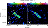Fig. A.1.

Velocity-integrated images of CH₃NH₂. The kinematic centre (Müller-Sánchez et al. 2010) is labelled by a white triangle. The regions where the spectra were extracted are shown by the black and white circles and are labelled in the left-most panel. The beam is depicted in the lower left corner of each plot. The scale bar of 100 pc corresponds to ∼6″. Left: Velocity-integrated map of CH₃NH₂ (1_1,5−1_0,5). Levels start at 3σ (1σ = 42 mJy beam⁻¹ km s⁻¹) with steps of 3σ. Right: Velocity-integrated map of CH₃NH₂ (3_−1,1−2_0,0). Levels start at 3σ (1σ = 42 mJy beam⁻¹ km s⁻¹) with steps of 3σ.

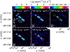Fig. A.2.

Same as Figure A.1 but for CH₂NH. Top Left: Velocity-integrated map of CH₂NH (3_1,2−2_1,1). Levels start at 3σ (1σ = 90 mJy beam⁻¹ km s⁻¹) with steps of 5σ. Bottom Left: Velocity-integrated map of CH₂NH (4_1,3−3_1,2). Levels start at 3σ (1σ = 78 mJy beam⁻¹ km s⁻¹) with steps of 8σ. Middle Top: Velocity-integrated map of CH₂NH (5_0,5−4_0,4). Levels start at 3σ (1σ = 140 mJy beam⁻¹ km s⁻¹) with steps of 8σ. Bottom Middle: Velocity-integrated map of CH₂NH (6_1,6−5_1,5). Levels start at 3σ (1σ = 210 mJy beam⁻¹ km s⁻¹) with steps of 5σ. Top Right: Velocity-integrated map of CH₂NH (8_1,7−8_0,8). Levels start at 3σ (1σ = 61 mJy beam⁻¹ km s⁻¹) with steps of 3σ.

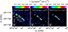Fig. A.3.

Same as Figure A.1 but for CH₃CHO. Left: Velocity-integrated map of CH₃CHO (1_1,5−1_0,5 (E+A)). Levels start at 3σ (1σ = 25 mJy beam⁻¹ km s⁻¹) with steps of 3σ. Middle: Velocity-integrated map of CH₃CHO (9_2,9−8_1,8 (E+A)). Levels start at 3σ (1σ = 55 mJy beam⁻¹ km s⁻¹) with steps of 3σ. Right: Velocity-integrated map of CH₃CHO (12_1,12−11_1,11 (E+A)). Levels start at 3σ (1σ = 36 mJy beam⁻¹ km s⁻¹) with steps of 3σ.

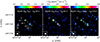Fig. A.4.

Same as Figure A.1 but for NH₂CHO. Left: Velocity-integrated map of NH₂CHO (8_0,8−7_0,7). Levels start at 3σ (1σ = 58 mJy beam⁻¹ km s⁻¹) with steps of 2σ. Middle: Velocity-integrated map of NH₂CHO (9_1,8−8_1,7). Levels start at 3σ (1σ = 52 mJy beam⁻¹ km s⁻¹) with steps of 3σ. Right: Velocity-integrated map of NH₂CHO (15_2,14−14_2,13). Levels start at 3σ (1σ = 78 mJy beam⁻¹ km s⁻¹) with steps of 3σ.

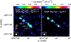Fig. A.5.

Same as Figure A.1 but for t-C₂H₅OH. Left: Velocity-integrated map of t-C₂H₅OH (6_4,2−5_3,3 and 6_4,3−5_3,2; blended together). Levels start at 3σ (1σ = 64 mJy beam⁻¹ km s⁻¹) with steps of 3σ. Right: Velocity-integrated map of t-C₂H₅OH (8_1,8−7_0,7). Levels start at 3σ (1σ = 26 mJy beam⁻¹ km s⁻¹) with steps of 3σ.

All Tables

Table 1.

Selected regions and coordinates.

In the text

Table 2.

Best fit results and 1σ confidence level range from the NLTE LVG analysis of CH₂NH.

In the text

All Figures

Fig. 1.

Overlap of contours corresponding to the velocity integrated species emission, ordered by their upper energy level, E_u. A spatial scale of 50 pc corresponds to ∼3″. The kinematic centre (α_ICRS = 00^h47^m33.14^s and δ_ICRS=−25°17′17.52″; Müller-Sánchez et al. 2010) is labelled by a filled black triangle. The black crosses mark the positions analysed in this work and correspond to GMC 7, GMC 6, pSSC 5 and pSSC 2. For reference, the position of GMC 3 and GMC 4 (Leroy et al. 2015) are indicated by magenta crosses in the panel a. The beam size if depicted in the lower left corner of each box. Contours of CH₃NH₂, CH₃CHO, CH₂NH, NH₂CHO, and C₂H₅OH are in grey, blue, orange, magenta, and green, respectively. a) Contour overlap of CH₃NH₂ (3_−1,1−2_0,0;E_u = 17 K) and CH₃CHO (1_1,5−1_0,5 (E+A); E_u = 19 K). Contours start at 3σ with steps of 3σ with 1σ = 42 and 25 mJy beam⁻¹ km s⁻¹, respectively. b) Contour overlap of CH₂NH (4_1,3−3_1,2;E_u = 39.8 K) with 1σ = 78 mJy beam⁻¹ km s⁻¹, CH₃CHO (9_2,9−8_1,8 (E+A); E_u = 43 K) with 1σ = 55 mJy beam⁻¹ km s⁻¹, NH₂CHO (8_0,8−7_0,7; E_u = 36 K) with 1σ = 58 mJy beam⁻¹ km s⁻¹, and t-C₂H₅OH (6₄−5₃; E_u = 37.7 K) with 1σ = 64 mJy beam⁻¹ km s⁻¹. Contours start at 3σ with steps of 3σ for CH₃CHO and t-C₂H₅OH, 8σ for CH₂NH, and 2σ for NH₂CHO. c) Contours overlap of CH₂NH (6_1,6−5_1,5;E_u = 69.6 K) with 1σ = 42 mJy beam⁻¹ km s⁻¹ and CH₃CHO (11_2,9−10_2,8 (E+A); E_u = 70.5 K) 1σ = 25 mJy beam⁻¹ km s⁻¹. Contours start at 3σ with steps of 5σ and 3σ for CH₂NH and CH₃CHO, respectively. d) Contour overlap of CH₂NH (8_1,7−8_0,8;E_u = 122.7 K), with 1σ = 61 mJy beam⁻¹ km s⁻¹ and NH₂CHO (15_2,14−14_2,13; E_u = 133.5 K) 1σ = 78 mJy beam⁻¹ km s⁻¹. Contours start at 3σ with steps of 2σ.

In the text

Fig. 2.

Rotational diagrams of each species towards GMC 6. Parameters E_u, N_u, and g_u are the level energy (with respect to the ground state), column density, and degeneracy of the upper level, respectively. The error bars on ln(N_u/g_u) include a calibration error of 15% (see Sect. 2). The blue (and orange if a second component is fitted) solid lines represent the best fits and the dashed grey lines are the extrapolations of the fit for the full range of E_u covered. The source size assumed is indicated for each component (see Sect. 4.1).

In the text

Fig. 3.

Line widths (FWHM; left-hand side) and peak velocities (V_peak; right-hand side) as a function of upper level energies (E_u) for CH₃OH (top panels), CH₃NH₂ (middle panels), and NH₂CHO (bottom panels) and for GMC 6 (filled green circles), pSSC 5 (filled magenta pentagons), and pSSC 2 (filled orange diamonds). The vertical dashed grey lines indicate where the deviation in the RDs occurs, i.e. ∼40 K, 30 K, and 60 K for CH₃CHO, CH₃NH₂, and NH₂CHO, respectively. Only the most clear Gaussian fits have been used (see text). If a second component has been identified in the RDs, it is shown in lighter color. Mean FWHM and V_peak are indicated on the plots by horizontal dashed lines accompanied with their corresponding values.

In the text

Fig. 4.

Derived rotational temperature (T_rot; top) and total column density (N_tot; bottom) for each species and region. The order of the regions follows the layout of the GMCs/SSCs of the CMZ from north-east to south-west as shown in Figure 1. Top: when two gas components were fitted in the RDs, the T_rot of the two components are indicated. Bottom: column densities derived for GMC scales (θ_s = 1.6″; bottom part) and pSSC scales (θ_s = 0.12″; top part). For the species (CH₂NH and C₂H₅OH) and region (GMC 7), where only one gas component was fitted, we calculated the column densities for the two scales. For the other regions and species, we attributed the first component to an emission coming from GMC scales and the second component to an emission coming from pSSC scales. In the cases of NH₂CHO and CH₃CHO, only one component was fitted for pSSC 2 and pSSC 5, respectively.

In the text

Fig. 5.

Volume density and kinetic temperature contour plots showing the results from the LVG analysis for CH₂NH towards GMC 7 (blue), GMC 6 (green), pSSC 5 (magenta), and pSSC 2 (orange). The contours show the 1σ solutions obtained for the minimum $χ_{r}^{2}$ $\chi ^2_r$ value in the column density parameter. The best fits are marked by black stars, while the best fit for the emission size (θ_s) are indicated in the bottom-left corner of the figure. The vertical grey line indicates the maximum temperature at which the rates are calculated.

In the text

Fig. 6.

Relation between the column densities of the iCOMs derived from the rotational diagrams at GMC scales (θ = 1.6″; left-hand side of the figure) and at pSSC scales (θ = 0.12″; right-hand side of the figure), for each region (GMC 7: blue; GMC 6: green; pSSC 5: magenta; pSSC 2: orange). Pearson's coefficient and p-values are indicated in the bottom right part of each plot. Dashed and full grey lines indicate abundance ratio factors. Panel k is highlighted as the correlation between CH₂NH and C₂H₅OH is the same at both GMC-scale and pSSC-scale. For reference for the location of each region, we added a map of the CH₂NH (4_1,3−3_1,2) transition in the bottom-left part of the figure.

In the text

Fig. 7.

Schematic (not to scale) of summarising the possible formation pathways and chemical links between the iCOMs (Sect. 5.1) and their emission origins (Sect. 5.2) within a GMC. The temperatures reported are averaged over the region but there can be variation from one region to another. We assume the size of a GMC is comparable or larger than the size of the ALCHEMI beam of 1.6″ (or ∼27 pc). Formation and chemical links: Sputtering from the ice grain mantle and gas phase formation pathways are both possible to explain the iCOM emission at GMC scales, whilst at SSC scales, the dust temperature can be high enough to allow thermal desorption. CH₃CHO and C₂H₅OH can also be chemically linked (i) both on the grain (with CH₃CHO as the precursor of C₂H₅OH) or via the Ethanol tree in the gas phase (with C₂H₅OH as a precursor for CH₃CHO). CH₃NH₂ and CH₂NH could be chemically linked (ii) by sharing similar precursors, both on the grain or in the gas phase (if the gas temperature is higher than 100 K; e.g. Halfen et al. 2013). Origin: At the scale of GMCs, the iCOMs are likely tracing large-scale shocks, due to either cloud-cloud collision (1) or shocks related to star formation activity (scenario 2a; see also Huang et al. 2023). At pSSC scales, iCOMs could trace either star formation-related heating process (scenario 2b; CH₃NH₂, NH₂CHO) and shocks (scenario 2a; CH₃CHO, CH₂NH, C₂H₅OH), associated or not (i.e. if cloud-cloud collision, scenario 1) with star formation.

In the text

Fig. A.1.

Velocity-integrated images of CH₃NH₂. The kinematic centre (Müller-Sánchez et al. 2010) is labelled by a white triangle. The regions where the spectra were extracted are shown by the black and white circles and are labelled in the left-most panel. The beam is depicted in the lower left corner of each plot. The scale bar of 100 pc corresponds to ∼6″. Left: Velocity-integrated map of CH₃NH₂ (1_1,5−1_0,5). Levels start at 3σ (1σ = 42 mJy beam⁻¹ km s⁻¹) with steps of 3σ. Right: Velocity-integrated map of CH₃NH₂ (3_−1,1−2_0,0). Levels start at 3σ (1σ = 42 mJy beam⁻¹ km s⁻¹) with steps of 3σ.

In the text

Fig. A.2.

Same as Figure A.1 but for CH₂NH. Top Left: Velocity-integrated map of CH₂NH (3_1,2−2_1,1). Levels start at 3σ (1σ = 90 mJy beam⁻¹ km s⁻¹) with steps of 5σ. Bottom Left: Velocity-integrated map of CH₂NH (4_1,3−3_1,2). Levels start at 3σ (1σ = 78 mJy beam⁻¹ km s⁻¹) with steps of 8σ. Middle Top: Velocity-integrated map of CH₂NH (5_0,5−4_0,4). Levels start at 3σ (1σ = 140 mJy beam⁻¹ km s⁻¹) with steps of 8σ. Bottom Middle: Velocity-integrated map of CH₂NH (6_1,6−5_1,5). Levels start at 3σ (1σ = 210 mJy beam⁻¹ km s⁻¹) with steps of 5σ. Top Right: Velocity-integrated map of CH₂NH (8_1,7−8_0,8). Levels start at 3σ (1σ = 61 mJy beam⁻¹ km s⁻¹) with steps of 3σ.

In the text

Fig. A.3.

Same as Figure A.1 but for CH₃CHO. Left: Velocity-integrated map of CH₃CHO (1_1,5−1_0,5 (E+A)). Levels start at 3σ (1σ = 25 mJy beam⁻¹ km s⁻¹) with steps of 3σ. Middle: Velocity-integrated map of CH₃CHO (9_2,9−8_1,8 (E+A)). Levels start at 3σ (1σ = 55 mJy beam⁻¹ km s⁻¹) with steps of 3σ. Right: Velocity-integrated map of CH₃CHO (12_1,12−11_1,11 (E+A)). Levels start at 3σ (1σ = 36 mJy beam⁻¹ km s⁻¹) with steps of 3σ.

In the text

Fig. A.4.

Same as Figure A.1 but for NH₂CHO. Left: Velocity-integrated map of NH₂CHO (8_0,8−7_0,7). Levels start at 3σ (1σ = 58 mJy beam⁻¹ km s⁻¹) with steps of 2σ. Middle: Velocity-integrated map of NH₂CHO (9_1,8−8_1,7). Levels start at 3σ (1σ = 52 mJy beam⁻¹ km s⁻¹) with steps of 3σ. Right: Velocity-integrated map of NH₂CHO (15_2,14−14_2,13). Levels start at 3σ (1σ = 78 mJy beam⁻¹ km s⁻¹) with steps of 3σ.

In the text

	Fig. A.5. Same as Figure A.1 but for t-C₂H₅OH. Left: Velocity-integrated map of t-C₂H₅OH (6_4,2−5_3,3 and 6_4,3−5_3,2; blended together). Levels start at 3σ (1σ = 64 mJy beam⁻¹ km s⁻¹) with steps of 3σ. Right: Velocity-integrated map of t-C₂H₅OH (8_1,8−7_0,7). Levels start at 3σ (1σ = 26 mJy beam⁻¹ km s⁻¹) with steps of 3σ.
In the text

Current usage metrics show cumulative count of Article Views (full-text article views including HTML views, PDF and ePub downloads, according to the available data) and Abstracts Views on Vision4Press platform.

Data correspond to usage on the plateform after 2015. The current usage metrics is available 48-96 hours after online publication and is updated daily on week days.

Initial download of the metrics may take a while.

[1] Aikawa, Y., Furuya, K., Yamamoto, S., & Sakai, N. 2020, ApJ, 897, 110 [Google Scholar]

[2] Ando, R., Nakanishi, K., Kohno, K., et al. 2017, ApJ, 849, 81 [CrossRef] [Google Scholar]

[3] Arce, H. G., Santiago-García, J., Jørgensen, J. K., Tafalla, M., & Bachiller, R. 2008, ApJ, 681, L21 [NASA ADS] [CrossRef] [Google Scholar]

[4] Arslan, Ö., Hocuk, S., Caselli, P., & Küçük, İ. 2023, MNRAS, 518, 2050 [Google Scholar]

[5] Baek, G., Lee, J. -E., Hirota, T., Kim, K. -T., & Kim, M. K. 2022, ApJ, 939, 84 [NASA ADS] [CrossRef] [Google Scholar]

[6] Barger, C. J., & Garrod, R. T. 2020, ApJ, 888, 38 [Google Scholar]

[7] Barone, V., Latouche, C., Skouteris, D., et al. 2015, MNRAS, 453, L31 [Google Scholar]

[8] Behrens, E., Mangum, J. G., Holdship, J., et al. 2022, ApJ, 939, 119 [NASA ADS] [CrossRef] [Google Scholar]

[9] Behrens, E., Mangum, J. G., Viti, S., et al. 2024, ApJ, 977, 38 [Google Scholar]

[10] Belloche, A., Müller, H. S. P., Menten, K. M., Schilke, P., & Comito, C. 2013, A&A, 559, A47 [NASA ADS] [CrossRef] [EDP Sciences] [Google Scholar]

[11] Belloche, A., Garrod, R. T., Müller, H. S. P., et al. 2019, A&A, 628, A10 [NASA ADS] [CrossRef] [EDP Sciences] [Google Scholar]

[12] Belloche, A., Maury, A. J., Maret, S., et al. 2020, A&A, 635, A198 [NASA ADS] [CrossRef] [EDP Sciences] [Google Scholar]

[13] Bendo, G. J., Beswick, R. J., D’Cruze, M. J., et al. 2015, MNRAS, 450, L80 [NASA ADS] [CrossRef] [Google Scholar]

[14] Bennett, C. J., Jamieson, C. S., Osamura, Y., & Kaiser, R. I. 2005, ApJ, 624, 1097 [Google Scholar]

[15] Beuther, H., Zhang, Q., Bergin, E. A., & Sridharan, T. K. 2009, AJ, 137, 406 [Google Scholar]

[16] Bianchi, E., Codella, C., Ceccarelli, C., et al. 2019, MNRAS, 483, 1850 [Google Scholar]

[17] Bianchi, E., López-Sepulcre, A., Ceccarelli, C., et al. 2022, ApJ, 928, L3 [NASA ADS] [CrossRef] [Google Scholar]

[18] Bisschop, S. E., Fuchs, G. W., van Dishoeck, E. F., & Linnartz, H. 2007, A&A, 474, 1061 [CrossRef] [EDP Sciences] [Google Scholar]

[19] Blake, G. A., Sutton, E. C., Masson, C. R., & Phillips, T. G. 1987, ApJ, 315, 621 [Google Scholar]

[20] Bocherel, P., Herbert, L., Rowe, B., et al. 1996, JPhCh, 100, 3063 [Google Scholar]

[21] Bøgelund, E. G., Barr, A. G., Taquet, V., et al. 2019a, A&A, 628, A2 [NASA ADS] [CrossRef] [EDP Sciences] [Google Scholar]

[22] Bøgelund, E. G., McGuire, B. A., Hogerheijde, M. R., van Dishoeck, E. F., & Ligterink, N. F. W. 2019b, A&A, 624, A82 [EDP Sciences] [Google Scholar]

[23] Bonfand, M., Belloche, A., Garrod, R. T., et al. 2019, A&A, 628, A27 [NASA ADS] [CrossRef] [EDP Sciences] [Google Scholar]

[24] Bouscasse, L., Csengeri, T., Wyrowski, F., Menten, K. M., & Bontemps, S. 2024, A&A, 686, A252 [NASA ADS] [CrossRef] [EDP Sciences] [Google Scholar]

[25] Bouvier, M., Viti, S., Behrens, E., et al. 2024, A&A, 689, A64 [NASA ADS] [CrossRef] [EDP Sciences] [Google Scholar]

[26] Brucato, J. R., Baratta, G. A., & Strazzulla, G. 2006, A&A, 455, 395 [NASA ADS] [CrossRef] [EDP Sciences] [Google Scholar]

[27] Burkhardt, A. M., Shingledecker, C. N., Le Gal, R., et al. 2019, ApJ, 881, 32 [Google Scholar]

[28] Burton, W. B., Elmegreen, B. G., Genzel, R., et al. 1992, Saas-Fee Advanced Course 21: The Galactic Interstellar Medium [Google Scholar]

[29] Busch, L. A., Belloche, A., Garrod, R. T., Müller, H. S. P., & Menten, K. M. 2024, A&A, 681, A104 [NASA ADS] [CrossRef] [EDP Sciences] [Google Scholar]

[30] Caselli, P., Hasegawa, T. I., & Herbst, E. 1993, ApJ, 408, 548 [Google Scholar]

[31] Ceccarelli, C., Maret, S., Tielens, A. G. G. M., Castets, A., & Caux, E. 2003, A&A, 410, 587 [NASA ADS] [CrossRef] [EDP Sciences] [Google Scholar]

[32] Ceccarelli, C., Caselli, P., Fontani, F., et al. 2017, ApJ, 850, 176 [NASA ADS] [CrossRef] [Google Scholar]

[33] Ceccarelli, C., Codella, C., Balucani, N., et al. 2023, in Protostars and Planets VII, eds. S. Inutsuka, Y. Aikawa, T. Muto, K. Tomida, & M. Tamura, ASP Conf. Ser., 534, 379 [NASA ADS] [Google Scholar]

[34] Chaabouni, H., Diana, S., Nguyen, T., & Dulieu, F. 2018, A&A, 612, A47 [NASA ADS] [CrossRef] [EDP Sciences] [Google Scholar]

[35] Charnley, S. B. 2004, Adv. Space Res., 33, 23 [NASA ADS] [CrossRef] [Google Scholar]

[36] Charnley, S. B., Tielens, A. G. G. M., & Millar, T. J. 1992, ApJ, 399, L71 [Google Scholar]

[37] Chen, Y., van Gelder, M. L., Nazari, P., et al. 2023, A&A, 678, A137 [NASA ADS] [CrossRef] [EDP Sciences] [Google Scholar]

[38] Chen, Y., Rocha, W. R. M., van Dishoeck, E. F., et al. 2024, A&A, 690, A205 [NASA ADS] [CrossRef] [EDP Sciences] [Google Scholar]

[39] Chuang, K. J., Fedoseev, G., Qasim, D., et al. 2020, A&A, 635, A199 [NASA ADS] [CrossRef] [EDP Sciences] [Google Scholar]

[40] Chuang, K. J., Jäger, C., Krasnokutski, S. A., Fulvio, D., & Henning, T. 2022, ApJ, 933, 107 [CrossRef] [Google Scholar]

[41] Codella, C., Ceccarelli, C., Caselli, P., et al. 2017, A&A, 605, L3 [NASA ADS] [CrossRef] [EDP Sciences] [Google Scholar]

[42] Codella, C., Ceccarelli, C., Bianchi, E., et al. 2020, A&A, 635, A17 [NASA ADS] [CrossRef] [EDP Sciences] [Google Scholar]

[43] Coletta, A., Fontani, F., Rivilla, V. M., et al. 2020, A&A, 641, A54 [NASA ADS] [CrossRef] [EDP Sciences] [Google Scholar]

[44] Costagliola, F., Sakamoto, K., Muller, S., et al. 2015, A&A, 582, A91 [NASA ADS] [CrossRef] [EDP Sciences] [Google Scholar]

[45] Csengeri, T., Belloche, A., Bontemps, S., et al. 2019, A&A, 632, A57 [NASA ADS] [CrossRef] [EDP Sciences] [Google Scholar]

[46] Danger, G., Borget, F., Chomat, M., et al. 2011, A&A, 535, A47 [NASA ADS] [CrossRef] [EDP Sciences] [Google Scholar]

[47] Dartois, E., Chabot, M., Id Barkach, T., et al. 2019, A&A, 627, A55 [NASA ADS] [CrossRef] [EDP Sciences] [Google Scholar]

[48] Dedes, C., Leurini, S., Wyrowski, F., et al. 2011, A&A, 526, A59 [NASA ADS] [CrossRef] [EDP Sciences] [Google Scholar]

[49] de Jesus, D. N., da Silva, J. M. B. A., Tejero, T. N., et al. 2021, MNRAS, 501, 1202 [Google Scholar]

[50] De Simone, M., Codella, C., Ceccarelli, C., et al. 2020, A&A, 640, A75 [NASA ADS] [CrossRef] [EDP Sciences] [Google Scholar]

[51] Dulieu, F., Nguyen, T., Congiu, E., Baouche, S., & Taquet, V. 2019, MNRAS, 484, L119 [NASA ADS] [CrossRef] [Google Scholar]

[52] Eibensteiner, C., Barnes, A. T., Bigiel, F., et al. 2022, A&A, 659, A173 [CrossRef] [EDP Sciences] [Google Scholar]

[53] Endres, C. P., Schlemmer, S., Schilke, P., Stutzki, J., & Müller, H. S. P. 2016, J. Mol. Spectr., 327, 95 [NASA ADS] [CrossRef] [Google Scholar]

[54] Enrique-Romero, J., Rimola, A., Ceccarelli, C., & Balucani, N. 2016, MNRAS, 459, L6 [Google Scholar]

[55] Enrique-Romero, J., Ceccarelli, C., Rimola, A., et al. 2021, A&A, 655, A9 [NASA ADS] [CrossRef] [EDP Sciences] [Google Scholar]

[56] Enrique-Romero, J., Rimola, A., Ceccarelli, C., et al. 2022, ApJS, 259, 39 [NASA ADS] [CrossRef] [Google Scholar]

[57] Faure, A., Lique, F., & Remijan, A. J. 2018, J. Phys. Chem. Lett., 9, 3199 [NASA ADS] [CrossRef] [Google Scholar]

[58] Fedoseev, G., Chuang, K. J., van Dishoeck, E. F., Ioppolo, S., & Linnartz, H. 2016, MNRAS, 460, 4297 [Google Scholar]

[59] Fedoseev, G., Qasim, D., Chuang, K. -J., et al. 2022, ApJ, 924, 110 [NASA ADS] [CrossRef] [Google Scholar]

[60] Ferrero, S., Zamirri, L., Ceccarelli, C., et al. 2020, ApJ, 904, 11 [NASA ADS] [CrossRef] [Google Scholar]

[61] Ferrero, S., Grieco, F., Ibrahim Mohamed, A. S., et al. 2022, MNRAS, 516, 2586 [CrossRef] [Google Scholar]

[62] Förstel, M., Bergantini, A., Maksyutenko, P., Góbi, S., & Kaiser, R. I. 2017, ApJ, 845, 83 [Google Scholar]

[63] Fuente, A., Cernicharo, J., Caselli, P., et al. 2014, A&A, 568, A65 [NASA ADS] [CrossRef] [EDP Sciences] [Google Scholar]

[64] García-Burillo, S., Martín-Pintado, J., Fuente, A., & Neri, R. 2000, A&A, 355, 499 [NASA ADS] [Google Scholar]

[65] Garrod, R. T., Widicus Weaver, S. L., & Herbst, E. 2008, ApJ, 682, 283 [Google Scholar]

[66] Garrod, R. T., Jin, M., Matis, K. A., et al. 2022, ApJS, 259, 1 [NASA ADS] [CrossRef] [Google Scholar]

[67] Goldsmith, P. F., & Langer, W. D. 1999, ApJ, 517, 209 [Google Scholar]

[68] Golshan, R. H., Sánchez-Monge, Á., Schilke, P., et al. 2024, A&A, 688, A3 [NASA ADS] [CrossRef] [EDP Sciences] [Google Scholar]

[69] Gorai, P., Bhat, B., Sil, M., et al. 2020, ApJ, 895, 86 [Google Scholar]

[70] Gorai, P., Law, C. -Y., Tan, J. C., et al. 2024, ApJ, 960, 127 [NASA ADS] [CrossRef] [Google Scholar]

[71] Gorski, M., Ott, J., Rand, R., et al. 2017, ApJ, 842, 124 [CrossRef] [Google Scholar]

[72] Gorski, M. D., Ott, J., Rand, R., et al. 2019, MNRAS, 483, 5434 [NASA ADS] [CrossRef] [Google Scholar]

[73] Gorski, M. D., Aalto, S., König, S., et al. 2023, A&A, 670, A70 [NASA ADS] [CrossRef] [EDP Sciences] [Google Scholar]

[74] Haasler, D., Rivilla, V. M., Martín, S., et al. 2022, A&A, 659, A158 [CrossRef] [EDP Sciences] [Google Scholar]

[75] Halfen, D. T., Ilyushin, V. V., & Ziurys, L. M. 2013, ApJ, 767, 66 [NASA ADS] [CrossRef] [Google Scholar]

[76] Harada, N., Martín, S., Mangum, J. G., et al. 2021, ApJ, 923, 24 [NASA ADS] [CrossRef] [Google Scholar]

[77] Harada, N., Martin, S., Mangum, J., et al. 2022, ApJ, 938, 80 [NASA ADS] [CrossRef] [Google Scholar]

[78] Harada, N., Meier, D. S., Martín, S., et al. 2024, ApJS, 271, 38 [NASA ADS] [CrossRef] [Google Scholar]

[79] Haupa, K. A., Joshi, P. R., & Lee, Y. -P. 2022, J. Chin. Chem. Soc., 69, 1159 [NASA ADS] [CrossRef] [Google Scholar]

[80] Henkel, C., Jacq, T., Mauersberger, R., Menten, K. M., & Steppe, H. 1987, A&A, 188, L1 [NASA ADS] [Google Scholar]

[81] Herbst, E., & van Dishoeck, E. F. 2009, ARA&A, 47, 427 [NASA ADS] [CrossRef] [Google Scholar]

[82] Holdship, J., Viti, S., Codella, C., et al. 2019, ApJ, 880, 138 [NASA ADS] [CrossRef] [Google Scholar]

[83] Holdship, J., Mangum, J. G., Viti, S., et al. 2022, ApJ, 931, 89 [NASA ADS] [CrossRef] [Google Scholar]

[84] Huang, K. -Y., Viti, S., Holdship, J., et al. 2023, A&A, 675, A151 [NASA ADS] [CrossRef] [EDP Sciences] [Google Scholar]

[85] Huang, K. Y., Abbink, D., Viti, S., & García-Burillo, S. 2024, A&A, 688, A130 [NASA ADS] [CrossRef] [EDP Sciences] [Google Scholar]

[86] Huang, K. Y., Behrens, E., Bouvier, M., et al. 2025, A&A, submitted [Google Scholar]

[87] Humire, P. K., Thiel, V., Henkel, C., et al. 2020, A&A, 642, A222 [NASA ADS] [CrossRef] [EDP Sciences] [Google Scholar]

[88] Humire, P. K., Henkel, C., Hernández-Gómez, A., et al. 2022, A&A, 663, A33 [NASA ADS] [CrossRef] [EDP Sciences] [Google Scholar]

[89] Ibrahim, M., Guillemin, J. -C., Chaquin, P., Markovits, A., & Krim, L. 2022, Physical Chemistry Chemical Physics (Incorporating Faraday Transactions), 24, 23245 [Google Scholar]

[90] Iodice, E., Arnaboldi, M., Rejkuba, M., et al. 2014, A&A, 567, A86 [NASA ADS] [CrossRef] [EDP Sciences] [Google Scholar]

[91] Jimenez-Serra, I. 2025, ArXiv e-prints [arXiv:2501.01782] [Google Scholar]

[92] Jin, M., & Garrod, R. T. 2020, ApJS, 249, 26 [Google Scholar]

[93] Jones, P. A., Burton, M. G., Tothill, N. F. H., & Cunningham, M. R. 2011, MNRAS, 411, 2293 [Google Scholar]

[94] Jørgensen, J. K., Müller, H. S. P., Calcutt, H., et al. 2018, A&A, 620, A170 [Google Scholar]

[95] Jørgensen, J. K., Belloche, A., & Garrod, R. T. 2020, ARA&A, 58, 727 [Google Scholar]

[96] Kahane, C., Ceccarelli, C., Faure, A., & Caux, E. 2013, ApJ, 763, L38 [CrossRef] [Google Scholar]

[97] Kim, Y. S., & Kaiser, R. I. 2011, ApJ, 729, 68 [NASA ADS] [CrossRef] [Google Scholar]

[98] Kishikawa, R., Harada, N., Saito, T., et al. 2025, PASJ, 77, 1 [Google Scholar]

[99] Krieger, N., Bolatto, A. D., Leroy, A. K., et al. 2020, ApJ, 897, 176 [Google Scholar]

[100] Kurtz, S., Cesaroni, R., Churchwell, E., Hofner, P., & Walmsley, C. M. 2000, in Protostars and Planets IV, eds. V. Mannings, A. P. Boss, & S. S. Russell, 299 [Google Scholar]

[101] Lamberts, T., Markmeyer, M. N., Kolb, F. J., & Kästner, J. 2019, ACS Earth Space Chem., 3, 958 [Google Scholar]

[102] Lee, C. -F., Codella, C., Li, Z. -Y., & Liu, S. -Y. 2019, ApJ, 876, 63 [NASA ADS] [CrossRef] [Google Scholar]

[103] Lefloch, B., Ceccarelli, C., Codella, C., et al. 2017, MNRAS, 469, L73 [Google Scholar]

[104] Leroy, A. K., Bolatto, A. D., Ostriker, E. C., et al. 2015, ApJ, 801, 25 [NASA ADS] [CrossRef] [Google Scholar]

[105] Leroy, A. K., Bolatto, A. D., Ostriker, E. C., et al. 2018, ApJ, 869, 126 [NASA ADS] [CrossRef] [Google Scholar]

[106] Levy, R. C., Bolatto, A. D., Leroy, A. K., et al. 2021, ApJ, 912, 4 [NASA ADS] [CrossRef] [Google Scholar]

[107] Li, C., Qin, S. -L., Liu, T., et al. 2024, MNRAS, 533, 1583 [NASA ADS] [CrossRef] [Google Scholar]

[108] Li, J., Shen, Z., Wang, J., et al. 2017, ApJ, 849, 115 [NASA ADS] [CrossRef] [Google Scholar]

[109] Li, J., Wang, J., Qiao, H., et al. 2020, MNRAS, 492, 556 [Google Scholar]

[110] Ligterink, N. F. W., Terwisscha van Scheltinga, J., Taquet, V., et al. 2018, MNRAS, 480, 3628 [Google Scholar]

[111] López-Sepulcre, A., Jaber, A. A., Mendoza, E., et al. 2015, MNRAS, 449, 2438 [CrossRef] [Google Scholar]

[112] López-Sepulcre, A., Balucani, N., Ceccarelli, C., et al. 2019, ACS Earth Space Chem., 3, 2122 [CrossRef] [Google Scholar]

[113] López-Sepulcre, A., Codella, C., Ceccarelli, C., Podio, L., & Robuschi, J. 2024, A&A, 692, A120 [NASA ADS] [CrossRef] [EDP Sciences] [Google Scholar]

[114] Lu, Y., Quan, D., Chang, Q., Chen, L. -F., & Li, D. 2025, ApJS, 277, 8 [Google Scholar]

[115] Mangum, J. G., Ginsburg, A. G., Henkel, C., et al. 2019, ApJ, 871, 170 [NASA ADS] [CrossRef] [Google Scholar]

[116] Maret, S., Hily-Blant, P., Pety, J., Bardeau, S., & Reynier, E. 2011, A&A, 526, A47 [NASA ADS] [CrossRef] [EDP Sciences] [Google Scholar]

[117] Martín, S., Mauersberger, R., Martín-Pintado, J., Henkel, C., & García-Burillo, S. 2006, ApJS, 164, 450 [Google Scholar]

[118] Martín, S., Krips, M., Martín-Pintado, J., et al. 2011, A&A, 527, A36 [NASA ADS] [CrossRef] [EDP Sciences] [Google Scholar]

[119] Martín-Doménech, R., Öberg, K. I., & Rajappan, M. 2020, ApJ, 894, 98 [Google Scholar]

[120] Martín, S., Mangum, J. G., Harada, N., et al. 2021, A&A, 656, A46 [NASA ADS] [CrossRef] [EDP Sciences] [Google Scholar]

[121] Matthews, H. E., Friberg, P., & Irvine, W. M. 1985, ApJ, 290, 609 [NASA ADS] [CrossRef] [Google Scholar]

[122] Mauersberger, R., Henkel, C., Walmsley, C. M., Sage, L. J., & Wiklind, T. 1991, A&A, 247, 307 [NASA ADS] [Google Scholar]

[123] McCarthy, P. J., van Breugel, W., & Heckman, T. 1987, AJ, 93, 264 [NASA ADS] [CrossRef] [Google Scholar]

[124] McCormick, A., Veilleux, S., & Rupke, D. S. N. 2013, ApJ, 774, 126 [NASA ADS] [CrossRef] [Google Scholar]

[125] Meier, D. S., Walter, F., Bolatto, A. D., et al. 2015, ApJ, 801, 63 [NASA ADS] [CrossRef] [Google Scholar]

[126] Mills, E. A. C., Gorski, M., Emig, K. L., et al. 2021, ApJ, 919, 105 [NASA ADS] [CrossRef] [Google Scholar]

[127] Mininni, C., Beltrán, M. T., Colzi, L., et al. 2023, A&A, 677, A15 [NASA ADS] [CrossRef] [EDP Sciences] [Google Scholar]

[128] Möller, T., Schilke, P., Sánchez-Monge, Á., & Schmiedeke, A. 2025, A&A, 693, A160 [NASA ADS] [CrossRef] [EDP Sciences] [Google Scholar]

[129] Molpeceres, G., Kästner, J., Herrero, V. J., Peláez, R. J., & Maté, B. 2022, A&A, 664, A169 [NASA ADS] [CrossRef] [EDP Sciences] [Google Scholar]

[130] Molpeceres, G., Furuya, K., & Aikawa, Y. 2024a, A&A, 688, A150 [NASA ADS] [CrossRef] [EDP Sciences] [Google Scholar]

[131] Molpeceres, G., Tsuge, M., Furuya, K., Watanabe, N., et al. 2024b, J. Phys. Chem. A, 128, 3874 [NASA ADS] [CrossRef] [Google Scholar]

[132] Müller, H. S. P., Schlöder, F., Stutzki, J., & Winnewisser, G. 2005, JMoSt, 742, 215 [Google Scholar]

[133] Muller, S., Beelen, A., Guélin, M., et al. 2011, A&A, 535, A103 [NASA ADS] [CrossRef] [EDP Sciences] [Google Scholar]

[134] Muller, S., Ubachs, W., Menten, K. M., Henkel, C., & Kanekar, N. 2021, A&A, 652, A5 [NASA ADS] [CrossRef] [EDP Sciences] [Google Scholar]

[135] Müller-Sánchez, F., González-Martín, O., Fernández-Ontiveros, J. A., Acosta-Pulido, J. A., & Prieto, M. A. 2010, ApJ, 716, 1166 [CrossRef] [Google Scholar]

[136] Nazari, P., Meijerhof, J. D., van Gelder, M. L., et al. 2022, A&A, 668, A109 [NASA ADS] [CrossRef] [EDP Sciences] [Google Scholar]

[137] Osterbrock, D. E. 1974, Astrophysics of Gaseous Nebulae (San Franciso: Freeman), A Series of Books in Astronomy and Astrophysics [Google Scholar]

[138] Paulive, A., Carder, J. T., & Herbst, E. 2022, MNRAS, 516, 4097 [Google Scholar]

[139] Pearson, J. C., Brauer, C. S., & Drouin, B. J. 2008, J. Mol. Spectr., 251, 394 [Google Scholar]

[140] Peng, Y., Liu, T., Qin, S. -L., et al. 2022, MNRAS, 512, 4419 [CrossRef] [Google Scholar]

[141] Perrero, J., Enrique-Romero, J., Martínez-Bachs, B., et al. 2022, ACS Earth and Space Chemistry, 6, 496 [Google Scholar]

[142] Perrero, J., Vitorino, J., Congiu, E., et al. 2024, Physical Chemistry Chemical Physics (Incorporating Faraday Transactions), 26, 18205 [Google Scholar]

[143] Pickett, H. M., Poynter, R. L., Cohen, E. A., et al. 1998, JQSRT, 60, 883 [NASA ADS] [CrossRef] [Google Scholar]

[144] Pérez-Beaupuits, J. P., Güsten, R., Harris, A., et al. 2018, ApJ, 860, 23 [Google Scholar]

[145] Qiu, J., Wang, J., Shi, Y., et al. 2018, A&A, 613, A3 [NASA ADS] [CrossRef] [EDP Sciences] [Google Scholar]

[146] Quénard, D., Jiménez-Serra, I., Viti, S., Holdship, J., & Coutens, A. 2018, MNRAS, 474, 2796 [Google Scholar]

[147] Raunier, S., Chiavassa, T., Duvernay, F., et al. 2004, A&A, 416, 165 [NASA ADS] [CrossRef] [EDP Sciences] [Google Scholar]

[148] Rekola, R., Richer, M. G., McCall, M. L., et al. 2005, MNRAS, 361, 330 [NASA ADS] [CrossRef] [Google Scholar]

[149] Requena-Torres, M. A., Martín-Pintado, J., Rodríguez-Franco, A., et al. 2006, A&A, 455, 971 [NASA ADS] [CrossRef] [EDP Sciences] [Google Scholar]

[150] Rico-Villas, F., Martin-Pintado, J., Gonzalez-Alfonso, E., Martin, S., & Rivilla, V. M. 2020, MNRAS, 491, 4573 [NASA ADS] [CrossRef] [Google Scholar]

[151] Rimola, A., Skouteris, D., Balucani, N., et al. 2018, ACS Earth Space Chem., 2, 720 [Google Scholar]

[152] Rivilla, V. M., García De La Concepción, J., Jiménez-Serra, I., et al. 2022a, Front. Astron. Space Sci., 9, 829288 [NASA ADS] [CrossRef] [Google Scholar]

[153] Rivilla, V. M., Jiménez-Serra, I., Martín-Pintado, J., et al. 2022b, Front. Astron. Space Sci., 9, 876870P [Google Scholar]

[154] Roberts, J. F., Rawlings, J. M. C., Viti, S., & Williams, D. A. 2007, MNRAS, 382, 733 [NASA ADS] [CrossRef] [Google Scholar]

[155] Rocha, W. R. M., van Dishoeck, E. F., Ressler, M. E., et al. 2024, A&A, 683, A124 [NASA ADS] [CrossRef] [EDP Sciences] [Google Scholar]

[156] Rodríguez-Rico, C. A., Goss, W. M., Zhao, J. H., Gómez, Y., & Anantharamaiah, K. R. 2006, ApJ, 644, 914 [CrossRef] [Google Scholar]

[157] Rosenberg, M. J. F., Kazandjian, M. V., van der Werf, P. P., et al. 2014, A&A, 564, A126 [NASA ADS] [CrossRef] [EDP Sciences] [Google Scholar]

[158] Ruaud, M., Loison, J. C., Hickson, K. M., et al. 2015, MNRAS, 447, 4004 [Google Scholar]

[159] Rubin, M., Altwegg, K., Balsiger, H., et al. 2019, MNRAS, 489, 594 [Google Scholar]

[160] Sakamoto, K., Mao, R. -Q., Matsushita, S., et al. 2011, ApJ, 735, 19 [CrossRef] [Google Scholar]

[161] Sanz-Novo, M., Rivilla, V. M., Jiménez-Serra, I., et al. 2024, ApJ, 965, 149 [Google Scholar]

[162] Sewiło, M., Indebetouw, R., Charnley, S. B., et al. 2018, ApJ, 853, L19 [CrossRef] [Google Scholar]

[163] Shimonishi, T., Tanaka, K. E. I., Zhang, Y., & Furuya, K. 2023, ApJ, 946, L41 [NASA ADS] [CrossRef] [Google Scholar]

[164] Sil, M., Gorai, P., Das, A., et al. 2018, ApJ, 853, 139 [NASA ADS] [CrossRef] [Google Scholar]

[165] Sivaramakrishnan, R., Su, M. -C., Michael, J. V., et al. 2009, J. Phys. Chem., A, 114, 755 [Google Scholar]

[166] Skouteris, D., Vazart, F., Ceccarelli, C., et al. 2017, MNRAS, 468, L1 [NASA ADS] [Google Scholar]

[167] Skouteris, D., Balucani, N., Ceccarelli, C., et al. 2018, ApJ, 854, 135 [NASA ADS] [CrossRef] [Google Scholar]

[168] Suzuki, T., Ohishi, M., Hirota, T., et al. 2016, ApJ, 825, 79 [NASA ADS] [CrossRef] [Google Scholar]

[169] Suzuki, T., Ohishi, M., Saito, M., et al. 2018, ApJS, 237, 3 [NASA ADS] [CrossRef] [Google Scholar]

[170] Suzuki, T., Majumdar, L., Goldsmith, P. F., et al. 2023, ApJ, 954, 189 [NASA ADS] [CrossRef] [Google Scholar]

[171] Tanaka, K., Mangum, J. G., Viti, S., et al. 2024, ApJ, 961, 18 [NASA ADS] [CrossRef] [Google Scholar]

[172] Tercero, B., Cuadrado, S., López, A., et al. 2018, A&A, 620, L6 [NASA ADS] [CrossRef] [EDP Sciences] [Google Scholar]

[173] Theule, P., Borget, F., Mispelaer, F., et al. 2011, A&A, 534, A64 [NASA ADS] [CrossRef] [EDP Sciences] [Google Scholar]

[174] Turner, B. E., Terzieva, R., & Herbst, E. 1999, ApJ, 518, 699 [NASA ADS] [CrossRef] [Google Scholar]

[175] Ulvestad, J. S., & Antonucci, R. R. J. 1997, ApJ, 488, 621 [NASA ADS] [CrossRef] [Google Scholar]

[176] Urso, R. G., Scirè, C., Baratta, G. A., et al. 2017, Physical Chemistry Chemical Physics (Incorporating Faraday Transactions), 19, 21759 [Google Scholar]

[177] van der Walt, S. J., Kristensen, L. E., Jørgensen, J., et al. 2021, A&A, 655, A86 [NASA ADS] [CrossRef] [EDP Sciences] [Google Scholar]

[178] Vasyunin, A. I., & Herbst, E. 2013, ApJ, 769, 34 [Google Scholar]

[179] Vazart, F., Calderini, D., Puzzarini, C., Skouteris, D., & Barone, V. 2016, J. Chem. Theory Comput., 12, 5385 [Google Scholar]

[180] Vazart, F., Ceccarelli, C., Balucani, N., Bianchi, E., & Skouteris, D. 2020, MNRAS, 499, 5547 [Google Scholar]

[181] Viti, S., Collings, M. P., Dever, J. W., McCoustra, M. R. S., & Williams, D. A. 2004, MNRAS, 354, 1141 [NASA ADS] [CrossRef] [Google Scholar]

[182] Widicus Weaver, S. L., Laas, J. C., Zou, L., et al. 2017, ApJS, 232, 3 [NASA ADS] [CrossRef] [Google Scholar]

[183] Woon, D. E. 2002, ApJ, 571, L177 [NASA ADS] [CrossRef] [Google Scholar]

[184] Xue, C., Remijan, A., Faure, A., et al. 2024, ApJ, 967, 164 [NASA ADS] [CrossRef] [Google Scholar]

[185] Yamamoto, S. 2017, Introduction to Astrochemsitry: chemical Evolution from Interstellar Clouds to Star and Planet Formation (New York: Springer) [Google Scholar]

[186] Yang, Y. -L., Sakai, N., Zhang, Y., et al. 2021, ApJ, 910, 20 [CrossRef] [Google Scholar]

[187] Zeng, S., Jiménez-Serra, I., Rivilla, V. M., et al. 2018, MNRAS, 478, 2962 [Google Scholar]

[188] Zeng, S., Zhang, Q., Jiménez-Serra, I., et al. 2020, MNRAS, 497, 4896 [NASA ADS] [CrossRef] [Google Scholar]

Complex organic molecules towards the central molecular zone of NGC 253

1. Introduction

2. Observations

3. Emission distribution and Gaussian line-fitting results

3.1. Emission distribution

3.2. Spectra and line parameters

4. Derivation of the physical parameters

4.1. Methodology

4.2. Rotational diagrams

4.2.1. Gaussian fits and temperature components

4.2.2. Results from the rotational diagrams

4.3. NLTE analysis: CH2NH

5. Discussion

5.1. Chemical link and formation pathways for iCOMs

5.1.1. CH3CHO and C2H5OH

5.1.2. NH2CHO

5.1.3. CH2NH and CH3NH2

5.2. Possible origins of the iCOMs in the CMZ of NGC 253

5.2.1. iCOMs production at GMC-scales

5.2.2. iCOMs production at pSSC-scale

5.3. Chemical variations across regions

5.3.1. The O- versus N-bearing dichotomy towards GMC 7

5.3.2. The CH3CHO – NH2CHO excitation condition anti-correlation in pSSC 5 and pSSC 2

6. Conclusions

Data availability

Acknowledgments

References

Appendix A: Integrated intensity images

All Tables

All Figures

4.3. NLTE analysis: CH₂NH

5.1.1. CH₃CHO and C₂H₅OH

5.1.2. NH₂CHO

5.1.3. CH₂NH and CH₃NH₂

5.3.2. The CH₃CHO – NH₂CHO excitation condition anti-correlation in pSSC 5 and pSSC 2