The most metal-poor tail of the Galactic halo: Hypothesis for its origin from precise spectral analysis

Riano E. Giribaldi; Laura Magrini; Martina Rossi; Anish M. Amarsi; Donatella Romano; Davide Massari

doi:10.1051/0004-6361/202453470

Home

All issues

Volume 698 (May 2025)

A&A, 698 (2025) A11

Full HTML

Open Access

Issue		A&A Volume 698, May 2025


Article Number		A11
Number of page(s)		22
Section		Galactic structure, stellar clusters and populations
DOI		https://doi.org/10.1051/0004-6361/202453470
Published online		03 June 2025

A&A, 698, A11 (2025)

The most metal-poor tail of the Galactic halo: Hypothesis for its origin from precise spectral analysis

Riano E. Giribaldi¹^★, Laura Magrini¹, Martina Rossi²^,3, Anish M. Amarsi⁴, Donatella Romano³ and Davide Massari³

¹ INAF – Osservatorio Astrofisico di Arcetri, Largo E. Fermi 5, 50125 Firenze, Italy
² Dipartimento di Fisica e Astronomia, Alma Mater Studiorum, Università di Bologna, Via Gobetti 93/2, 40129 Bologna, Italy
³ INAF, Osservatorio di Astrofisica e Scienza dello Spazio, Via Gobetti 93/3, 40129 Bologna, Italy
⁴ Theoretical Astrophysics, Department of Physics and Astronomy, Uppsala University, Box 516 SE-751 20 Uppsala, Sweden

^★ Corresponding author: riano.escategirbaldi@inaf.it; rianoesc@gmail.com

Received: 16 December 2024
Accepted: 24 March 2025

Abstract

Context. The origin of the Galactic halo is one of the fundamental topics linking the study of galaxy formation and evolution to cosmology.

Aims. Our goal is to derive precise and accurate stellar parameters, Mg abundances, and ages for a sample of metal-poor stars with [Fe/H] < − 2 dex from high signal-to-noise and high spectral resolution archival spectra.

Methods. We derived effective temperatures from Hα profiles using three-dimensional non-local thermodynamic equilibrium (3D NLTE) models, and surface gravities and ages from isochrone fitting based on Gaia data. Iron abundances were derived in one-dimensional (1D) NLTE, while Mg abundances were derived in 1D LTE, 1D NLTE, 3D LTE, and 3D NLTE to show the increasing level of accuracy.

Results. The sample stars show a tight trend in the [Mg/Fe] versus [Fe/H] plane with a knee located at [Fe/H] ≈ − 2.8 dex, which indicates a low level of stochasticity at the sampled metallicities in this kind of population. Their location in the Lindblad diagram confirms that they belong to the Galactic halo, but does not show a distinct clustering that might be expected for a merger with a single low-mass galaxy. Comparison with chemical evolution models is also not fully definitive on whether the sample stars were born in situ or in accreted low-mass galaxy mergers.

Conclusions. Overall, we find two plausible explanations for the chemical sequence traced by the stars in the [Mg/Fe] versus [Fe/H] plane. One is that the sample stars originated in the already formed Milky Way, which at that time (12.5 Gyr ago) was already the main galaxy of its Local Group surroundings. Another explanation is that the sample stars originated in several small galaxies with similar properties, which later merged with the Galaxy. Only accurate spectroscopic analysis such as that done here can reveal trustworthy chemical diagrams required to observe the traces of the Galaxy evolution. Increasing the sample size and the analysis of other elements are required to differentiate between the two hypotheses.

Key words: stars: abundances / stars: fundamental parameters / Galaxy: abundances / Galaxy: evolution / Galaxy: formation / Galaxy: halo

© The Authors 2025

Open Access article, published by EDP Sciences, under the terms of the Creative Commons Attribution License (https://creativecommons.org/licenses/by/4.0), which permits unrestricted use, distribution, and reproduction in any medium, provided the original work is properly cited.

This article is published in open access under the Subscribe to Open model. Subscribe to A&A to support open access publication.

1 Introduction

The evolutionary path of the Milky Way has been strongly influenced by several mergers that happened in the past (see e.g. Kruijssen et al. 2020; Malhan et al. 2022). At least one was a major accretion event that occurred about 9.5 Gyr ago with the Gaia-Enceladus or Gaia-Sausage progenitor (Belokurov et al. 2018; Helmi et al. 2018; Gallart et al. 2019; Massari et al. 2019; Belokurov et al. 2020; Borre et al. 2022; Giribaldi & Smiljanic 2023). This scenario is supported by a great deal of evidence of the observational properties of possible members belonging to the remnants of merging galaxies, such as chemical abundances from stellar spectra, and kinematic properties derived from radial velocities and from proper motions (e.g. Nissen & Schuster 2010; Myeong et al. 2019; Monty et al. 2020; Bonaca et al. 2020; Feuillet et al. 2021; da Silva & Smiljanic 2023; Ceccarelli et al. 2024). Precise and accurate chemical and kinematic data are required as constraints to develop and improve cosmological and numerical chemo-dynamical simulations of galaxy formation (e.g. Brook et al. 2003; Grand et al. 2020; Rey et al. 2023), built in the frameworks of the two compelling scenarios: monolithic collapse (e.g. Eggen et al. 1962) and hierarchical accretion (Searle & Zinn 1978). In particular, the presence of the remnant of the Gaia-Enceladus merger in the nearby halo is characterised by a different pattern with respect to the Milky Way in situ populations in several chemical planes, such as [Mg¹/Fe]² versus [Fe/H], [Ni/Fe] versus [(C+N)/O], and [Mg/Mn] versus [Al/Fe] (e.g. Feuillet et al. 2021; Montalbán et al. 2021; Horta et al. 2021; Giribaldi & Smiljanic 2023); these differences have been exhaustively explored thanks to the observations carried out with the large spectroscopic surveys, such as the Apache Point Observatory Galactic Evolution Experiment (APOGEE, Abdurro’uf et al. 2022) and the Galactic Archaeology with HERMES survey (GALAH, De Silva et al. 2015). Although these surveys are reasonably sampled down to [Fe/H] ∼− 1.5 dex, they are moderately limited for [Fe/H] ≲ −1.5 dex, and severely limited for [Fe/H] ≲ −2 dex. Nevertheless, a dedicated search for the oldest most metal-poor stars by the Pristine survey (Starkenburg et al. 2017) is progressively pushing these limits. In addition, it is worth mentioning the Measuring at Intermediate Metallicity Neutron Capture Element (MINCE) survey (Cescutti et al. 2022; François et al. 2024), which is currently acquiring high-resolution spectra of metal-poor stars with several facilities in diverse observatories, with the aim of studying the nucleosynthesis processes at early stages of the Milky Way assembling.

These are precisely the most metal-poor stars that allow us to investigate the most distant past of our Galaxy, probably dominated by a large number of mergers (see e.g. Witten et al. 2024). While some orbital properties are likely to be lost when tracing back in time (e.g. Jean-Baptiste et al. 2017), chemical properties, such as photospheric abundance ratios, remain largely preserved. Detailed chemical analyses of a few hundred stars with −4 ≲ [Fe/H] ≲ −3 dex and a few dozen with [Fe/H] ≲ −4 have been done via moderate-resolution spectroscopy (e.g. Cayrel et al. 2004; Norris et al. 2013; Yong et al. 2013; Aoki et al. 2013; Cohen et al. 2013; Jacobson et al. 2015; Norris et al. 2007; Caffau et al. 2012; Spite et al. 2013; Hansen et al. 2013; Frebel et al. 2005; Aoki et al. 2006; Christlieb et al. 2002; Keller et al. 2014; Aguado et al. 2019, 2022; Arentsen et al. 2023; Sestito et al. 2023, among other works). The vast majority of these stars are red giants, as exploring distant environments, such as the Galaxy halo and bulge, requires the observation of the brightest objects. However, there are also observations of several dwarf stars in the sample of the nearest stars.

For the main stellar populations of the Milky Way, such as thin and thick discs, the halo, and the bulge, the [Mg/Fe] versus [Fe/H] (or alternatively versus [Be/H]) diagram proved to be a key tool for identifying the different origins of the various populations and their star formation history and efficiency, even in the metal-poor regime (e.g. Smiljanic et al. 2009; Nissen & Schuster 2010). Most of the literature spectroscopic works adopted the standard spectroscopic analysis: one-dimensional (1D) hydrostatic model atmospheres and the assumption of local thermodynamic equilibrium (LTE). Their results usually display a substantial scatter in the [Mg/Fe] versus [Fe/H] diagram. Only a few works analysing metal-poor stars ([Fe/H] < −2 dex) indicate a flat trend with dispersions compatible with the errors of individual [Mg/Fe] measurements (see e.g. François et al. 2004; Arnone et al. 2005; Andrievsky et al. 2010; Aoki et al. 2013; Jacobson et al. 2015). Arnone et al. (2005) analysed 23 dwarfs and obtained a scatter of 0.06 dex consistent with star-to-star errors. This suggests that the typical [Mg/Fe] scatter observed in the literature with 1D-LTE analysis is mainly dominated by data and modelling errors. In this respect, Andrievsky et al. (2010) showed that 1D with non-LTE (NLTE) line modelling might alleviate the [Mg/Fe] offset of ∼0.2 dex between giants and dwarfs displayed by their 1D LTE modelling, and thus it can significantly decrease the scatter and dispersion. Therefore, it is evident that in the analysis of metal-poor stars, NLTE effects must be considered (see e.g. Sitnova et al. 2019).

In addition, the implementation of three-dimensional (3D) model atmospheres for line synthesis (under NLTE) in the most metal-poor regime is becoming even more necessary so as to obtain accurate effective temperatures of FGK type stars; and also to obtain accurate individual element abundances. For the former, efforts over the years of testing diverse model recipes (e.g. Vidal et al. 1970; Stehlé & Hutcheon 1999; Barklem et al. 2000, 2002; Barklem 2007; Allard et al. 2008; Ludwig et al. 2009; Pereira et al. 2013; Amarsi et al. 2018) have indicated that the spectral synthesis of Balmer line profiles under 3D NLTE (Amarsi et al. 2018) can accurately reproduce the observational profiles of dwarfs and giants from their actual³ T_eff values (Giribaldi et al. 2021, 2023). Once stars are benchmarked by those methods, the differential approach can be used with confidence for stars with similar parameters, as done by Reggiani et al. (2016) and Reggiani & Meléndez (2018), for instance. The latter is related to the line spectral synthesis of some elements: the abundances measured under the 3D NLTE synthesis may drastically change patterns of element ratios (e.g. Amarsi et al. 2019) or even emphasise the pattern separation of stellar populations (e.g. Matsuno et al. 2024).

Recent findings (Horta et al. 2023) have highlighted that the time of accretion and the stellar mass of an accreted satellite are key factors in shaping the spatial distribution, orbital energy, and chemical compositions of stellar debris. In particular, in the inner halo (R_GC < 30 kpc), where phase mixing dominates, the debris from both lower- and higher-mass satellites are expected to be fully spatially blended with stars formed in situ. Despite this extensive mixing, the persistence of distinct chemical signatures might provide insight into the assembly history of the Milky Way. For this work, we therefore propose to reanalysed a sample of metal-poor stars with state-of-the-art spectral analysis tools, including whenever possible 3D and NLTE, in order to reveal their pattern in the [Mg/Fe] versus [Fe/H] plane and, from it, to infer their origin. We compared our results with chemical evolution models, which are also discussed in the light of recent chemo-dynamical simulations.

The paper is structured as follows. In Section 2 we present our three samples, whereas in Section 3 we describe how we derived the stellar parameters. In Section 4 we report how the abundances of Mg are computed in the various approximations. In Section 5 we provide our results on the chemical and kinematic properties of the samples. We discuss our results in Section 6, and make a comparison with two chemical evolution models, and we provide a summary and our conclusions in Section 7.

2 Data and sample

Our sample includes halo stars in the metal-poor regime ([Fe/H] < −2 dex), belonging to three different samples: precision samples I and II, and the Gaia-ESO sample. Our targets are selected to have high-resolution and high S/N spectra so that it is possible to derive precise abundances and to constrain the [Mg/Fe]–[Fe/H] pattern. In what follows, we briefly describe our three samples.

Precision sample I: It is composed of stars selected from Giribaldi & Smiljanic (2023, Paper I henceforth). It consists of dwarf FGK stars: 15 over 48 stars from Giribaldi et al. (2021) named TITANS I. Their parameters were derived from Ultraviolet and Visual Echelle Spectrograph (UVES, Dekker et al. 2000) spectra of the European Southern Observatory (ESO), with resolution higher than R = λ/Δλ = 40 000. In most cases, for the element abundance analyses, we combined spectra of the same resolution to optimise the S/N. When available, also spectra taken by the High Accuracy Radial velocity Planet Searcher (HARPS of R = 115 000, Mayor et al. 2003) and the Echelle SPectrograph for Rocky Exoplanets and Stable Spectroscopic Observation (ESPRESSO of R = 190 000, Pepe et al. 2021) instruments were used. Specific resolution and S/N values are listed in Table A.2. The stars in the TITANS I sample are accurate templates, since their spectroscopic T_eff and parallax-based log g are compatible with values determined by fundamental methods: interferometry and InfraRed Flux Method (IRFM). Paper I also includes 212 stars from the GALAH DR3 catalogue (Buder et al. 2021), but none has [Fe/H] < −2, therefore GALAH stars are absent in this sample; they are used only as reference to display the concentration of the stellar populations in chemical and kinematic diagrams. We include five additional new dwarf stars selected from the sample of Meléndez et al. (2010). These stars allow us to cover the [Fe/H] range between −3 and −2.5 dex, improving the TITANS I sub-sample. These are BPS BS16968−0061, BPS CS22177−0009, BPS CS22953−0037, and BPS CS29518−0043, which have UVES archival spectra, obtained with a resolving power R ∼42 000 and with 100 < S/N < 170. Their spectra fulfil our request to embrace the Hα line profiles without distortions of artificial or physical origin. Respectively, imperfect blaze subtraction and artefacts such as ripple-like patterns due to imperfect order merging (Škoda & Šlechta 2004; Škoda et al. 2008), or flux emission at either of the two wings (e.g. Fig. A.3). We also analysed the star BPS BS16023−0046 from Meléndez et al. (2010), which has a spectrum with S/N ∼50. Since its spectrum has a very weak magnesium line (at 5528 Å), which leads to an uncertain abundance, we included this star in the lower-precision sample, that is together with the Gaia-ESO sample. Stars with spectra with such distortions in all samples are indicated in Table A.2.

Precision sample II: It contains 13 red giants from the TITANS II (Giribaldi et al. 2023) sample with [Fe/H] < −2 dex and spectra of S/N > 140. Since red giants are cooler than main sequence FGK dwarf stars, their metal lines are more prominent and permit the determination of the abundances in very metal-poor stars with higher precision. For a more homogeneous sample, we excluded the handful of Carbon-Enhanced Metal-Poor (CEMP) giants present in the TITANS II set. The stars in Precision sample II are also accurate templates because their atmospheric parameters are compatible with those from fundamental methods, as described in the analysis of Giribaldi et al. (2023).

Gaia-ESO sample: The Gaia-ESO survey (Randich et al. 2022; Gilmore et al. 2022) is a large public spectroscopic survey that observed for 340 nights at the Very Large Telescope (VLT) from the end of 2011 to 2018. It gathered ∼190 000 spectra, for nearly 115 000 targets belonging to all the main Galactic populations. It is still the only stellar survey using 8 m class telescopes, with the explicit aim of being complementary to the data obtained by the Gaia satellite (see e.g. Van der Swaelmen et al. 2024, for a thorough comparison with Gaia spectroscopic results). Gaia-ESO observed its targets at two different R: the medium-resolution sample was observed with GIRAFFE at R ∼20 000 and the high-resolution sample with UVES at R ∼47 000. From this latter sample, we selected very metal-poor field stars ([Fe/H] < −2 and with GES_FLD=GE_MW) whose stellar parameters and abundances are available in the final data release DR 5.1 (Hourihane et al. 2023). This sample is rather limited in number because the Gaia-ESO target selection did not favour halo populations (Stonkute? et al. 2016). We obtained their reduced spectra from the ESO archive, and we consistently re-analysed them as our Precision samples. Our Gaia-ESO sample contains 27 stars with [Fe/H] < −2 dex, from which we discarded three stars because our method failed to retrieve reliable parameters from their spectra. One of these stars (GES J13301360-4346323) has a very narrow Hα line with a small flux emission in one of its wings, we suspect it may be a giant with log g < 1 dex. Another star (GES J08192562-1405040) is located at the base of the red giant branch, and although it has a spectrum with S/N = 50, its Fe lines appear at the limit of detection. We also excluded GES J14205624-3701526 from our sample because its Mg line at 5528 Å is affected by an artefact. We added to the Gaia-ESO sample one star from the ESO archive, as described above (see Precision sample I).

General properties: Figures 1 and 2 show some general properties of the overall sample. Figure 1 displays the distribution of the S/N of our sample spectra. The spectra in the Precision samples I and II, which together contain 32 stars, are those with the highest S/N ≳ 100, whereas the spectra in the Gaia-ESO sample have S/N ∼ 50. The stars in this latter sample are usually fainter, with 12.5 ≲ G ≲ 15, whereas the Precision samples mostly have brighter stars.

Figure 2 shows the distribution of the stars in the frame Galactocentric distance (R_GC) versus heights on the Galactic plane (Z). It shows that 72% (23 of 32) of the stars in the Precision samples I and II are concentrated in the solar neighbourhood, defined here as a squared box of 3 kpc with the Sun at its centre. Only five of 23 stars of the Gaia-ESO sample are located in the solar neighbourhood, while 10 of them lie in the direction of the Galactic centre. As a reference background, a colour-coded density dispersion of the 6250 stars selected by Giribaldi & Smiljanic (2023) is displayed in the figure.

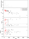Fig. 1

Observational properties of the full sample. The top panel displays a histogram of the S/N. From the second panel downwards, G magnitude, log g, and [Fe/H] are plotted as a function of the S/N. Precision samples I and II, and the Gaia-ESO sample are represented by different symbols. In the third panel, the dotted line displays the division between dwarfs and giants. The surface gravity and [Fe/H] values are those listed in Table A.3.

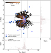Fig. 2

Spatial distribution of our sample stars with respect to the Galaxy centre. The colours of the symbols distinguish the Precision samples (empty circles) and the Gaia-ESO sample (filled blue circles). A sample of 6250 halo stars of the GALAH survey are plotted as reference background, colour-coded by density. The dotted lines indicate Z_⊙ ± 1.5 and R_GC _⊙ ± 1.5 kpc. Histograms of the distribution in R_GC and Z of the full and the Precision samples I and II are displayed.

3 Atmospheric parameters and ages

In this section, we describe the methodology used for the determination of atmospheric parameters and ages. The method changes slightly depending on the S/N of the spectrum and whether dwarf or giant stars are analysed. Figure 3 shows our sample stars in the Kiel Diagram.

Precision sample I: The determination of the atmospheric parameters of dwarf stars is described in Giribaldi et al. (2021), and details of the determination of their ages are given in Giribaldi & Smiljanic (2023). In the present work, we adopted the values obtained in such papers. Here we briefly recall the used method: the sample has two sets of accurate and compatible temperatures: one derived by IRFM (Casagrande et al. 2010, $T_{eff}^{IRFM}$ $T_\frame{\frame{\text{eff~}}}^\frame{\frame{\text{IRFM~}}}$ ) and with the 3D NLTE synthetic profiles of Amarsi et al. (2018). We combine the two sets of temperatures as described below to improve the precision to a few Kelvin. Surface gravity and age are based on isochrone fitting (using Yonsey-Yale, Kim et al. 2002; Yi et al. 2003) using the frequentist approach implemented in the q² code (Ramírez et al. 2013), the formalism of which is exposed in Meléndez et al. (2012). We used as inputs the Gaia parallax, [Fe/H], extinction-corrected V, and T_eff; obtaining outputs of typical precisions of 0.05 dex and 0.6 Gyr in log g and age, respectively. Figure 4 shows a histogram of the ages of all dwarf stars in Table A.3. Metallicity is based on spectral synthesis of weak lines with reduced equivalent width, REW < 5. The line list used is given in Table A.1.

We include in this sample five very metal-poor dwarf stars studied by Meléndez et al. (2010), as described above. To improve the T_eff(Hα) precision, we degraded the spectral resolution from R ∼ 42 000 to R ∼ 25 000, this way we duplicate the S/N. Figure A.1 shows the fits done as in Giribaldi et al. (2019) with the synthetic 3D NLTE line profiles.

Some stars in the sample do not have $T_{eff}^{IRFM}$ $T_\frame{\frame{\text{eff~}}}^\frame{\frame{\text{IRFM~}}}$ ⁴, for them we derive photometric temperatures $(T_{eff .}^{phot})$ $(T_\frame{\frame{\text{eff}}\frame{\text{.~}}}^\frame{\frame{\text{phot~}}})$ using Gaia colour-T_eff relations calibrated with IRFM determinations (Casagrande et al. 2021). We only use BP − RP and G − BP colours, as G − BR was observed to produce outcomes slightly biased to cooler values (Fig. 10 in Giribaldi et al. 2023). $T_{eff}^{phot}$ $T_\frame{\frame{\text{eff~}}}^\frame{\frame{\text{phot~}}}$ is given by the weighted average of the outcomes from each colour-T_eff relation, where the weights (ω_i) are the squared inverse of their internal errors. These errors are obtained by randomising [Fe/H] and log g within Gaussian distributions of σ equal to typical uncertainties; for this sample σ = 0.05 dex. The internal error of $T_{eff}^{phot}$ $T_\frame{\frame{\text{eff~}}}^\frame{\frame{\text{phot~}}}$ is obtained by the formula: $δ T = \sqrt{\frac{\sum_{i} {(T - T_{i})}^{2} ω_{i}}{\frac{(n - 1)}{n} \sum_{i} ω_{i}}}$ $\delta T = \sqrt \frame{\frac{\frame{\mathop \sum \limits_i \frame{\frame{\left(\nolbrace \frame{T - \frame{T_i}} \norbrace\right)}^2}\frame{\omega _i}}}{\frame{\frac{\frame{(n - 1)}}{n}\mathop \sum \limits_i \frame{\omega _i}}}}$ (1)

where T is the averaged value, T_i represents the temperature from each colour-T_eff relation, ω_i is the corresponding weight, and n is the number of quantities averaged. The total error of $T_{eff}^{phot}$ $T_\frame{\frame{\text{eff~}}}^\frame{\frame{\text{phot~}}}$ is obtained by adding in quadrature the internal error with the error induced by the extinction uncertainty $(δ T_{eff}^{E (B - V)})$ $(\delta T_\frame{\frame{\text{eff~}}}^\frame{E(B - V)})$ and the precision of the colour calibrations (∼ 60 K, see Table 1 in Casagrande et al. 2021).

For Precision samples I and II, the final T_eff is given by the weighted average of Teff(Hα) and either interferometric temperatures $(T_{eff}^{int}), T_{eff}^{IRFM}, or T_{eff}^{phot}$ $(T_\frame{\frame{\text{eff~}}}^\frame{\frame{\text{int~}}}),T_\frame{\frame{\text{eff~}}}^\frame{\frame{\text{IRFM~}}},\frame{\text{or}}T_\frame{\frame{\text{eff~}}}^\frame{\frame{\text{phot~}}}$ ; the two first ( $T_{eff}^{int}$ $T_\frame{\frame{\text{eff~}}}^\frame{\frame{\text{int~}}}$ and $T_{eff}^{IRFM}$ $T_\frame{\frame{\text{eff~}}}^\frame{\frame{\text{IRFM~}}}$ ) are preferred over the last because they are more fundamental. The internal error of the final T_eff is obtained by Eq. (1). Table A.3 lists the atmospheric parameters of all stars, whereas Table A.2 lists the temperatures derived by each method.

Precision sample II: The determination of the atmospheric parameters of giants is described in detail and tested in Giribaldi et al. (2023). Their method consists on deriving T_eff by Hα profiles with the same family of 3D NLTE models used for Precision Sample I. We derive $T_{eff}^{phot}$ $T_\frame{\frame{\text{eff~}}}^\frame{\frame{\text{phot~}}}$ for these stars as done with Precision Sample I. Therefore, here we assume T_eff equals the weighted average of both quantities. The star HD 122563 is an exception, for which T_eff(Hα) and $T_{eff}^{int}$ $T_\frame{\frame{\text{eff~}}}^\frame{\frame{\text{int~}}}$ were averaged, as the latter is available in Karovicova et al. (2020). The method in Giribaldi et al. (2023) relies on the Mg I b triplet lines to derive log g compatible with asteroseismologic measurements, and it derives [Fe/H] by spectral synthesis from weak Fe II lines with REW < −5 considering NLTE corrections. We avoid calculating the ages of the giants because of the high degeneracy between isochrones in the region where they are located in the Kiel diagram.

In addition, in the present work we refined the determination of [Fe/H] by performing line synthesis under NLTE using the radiative transfer code Turbospectrum 2020⁵ (Gerber et al. 2023) with MARCS model atmospheres (Gustafsson et al. 2008). We considered the atomic parameters from Heiter et al. (2021) and the iron NLTE departure coefficients based on the model atom developed in Bergemann et al. (2012) and Semenova et al. (2020). We compiled a Fe line list initially selecting lines from Jofré et al. (2014), Dutra-Ferreira et al. (2016), and Meléndez & Barbuy (2009). Then, we made preliminary selections of new lines by visual inspection by comparing observational with synthetic spectra. Our criterion consists in selecting all lines away from regions seriously contaminated by other spectral characteristics. We finally cleaned this selection by removing lines with excitation potential (χ_ex) lower than 1.4 eV to avoid sources of overestimation (e.g. Sitnova et al. 2015, 2024). The line list is presented in Table A.1.

Since for several stars, Mg abundances will be derived from saturated lines, it is important to fine tune v_mic with similarly strong lines. We did it under NLTE assuming the [Fe/H] balance of lines with REW < −4.8; [Fe/H] and associated microturbulent velocity (v_mic) values are listed in Table A.3. From the analysis of the spectra of giant stars we found that the excitation equilibrium of iron is systematically retrieved under NLTE. See Fig. A.4, where the excitation equilibrium is recovered from [Fe/H] and v_mic values in Giribaldi et al. (2023). Exceptions found are the stars BD −18 5550, BPS CS 22891 − 209, and BPS CS 29518 − 051, whose former log g values (derived from Mg I b triplet lines) were biased likely because of the interdependence with the Mg abundance. For these stars, we derive log g assuming the excitation equilibrium of iron under NLTE. Later, after Mg abundance is derived, we tune log g from the Mg I b triplet; this way, all stars in the sample share the same log g accuracy and precision. We show the determination of log g of the star BPS CS 29518−051 in Fig. A.2 as an example.

The ionisation equilibrium under NLTE differs from what was found under LTE conditions: a general offset of 0.1-0.2 dex between Fe I and Fe II exists in LTE that is removed in NLTE. As example, we show the case of the star HD 122563 in Figure 5, where the offset between both Fe species under LTE is visible.

This again shows the importance of accurate T_eff determination and NLTE corrections for metal poor giants. In addition, we found that our sample of giants have v_mic ∼ 1.2 ± 0.3 km s⁻¹ (median and standard deviation, respectively), which may be somewhat lower than typical values in the literature derived under LTE for giant stars (e.g. François et al. 2007; Jofré et al. 2014). A different micro-turbulence value may have important effects in the determination of abundances (see e.g. Baratella et al. 2020, 2021). In the case of HD 122563 shown in the figure, the LTE analysis provides a v_mic value of 1.6 km s⁻¹, which is 0.4 km s⁻¹ higher than in NLTE. This higher value of v_mic produces a [Fe/H] value biased by −0.15 dex.

Gaia-ESO sample: Most Gaia-ESO stars are giants, with typical S/N 50. We derive their T_eff same way as done for Precision Sample II. Several of their spectra present Hα profiles with distortions (e.g. Fig. A.3); the last column in Table A.2 indicates the stars with such problems. For the corresponding stars, we only derive $T_{eff}^{phot}$ $T_\frame{\frame{\text{eff~}}}^\frame{\frame{\text{phot~}}}$ from BP RP and G − BP colours. This temperature scale depends mildly on log g and [Fe/H], and strongly on the extinction⁶ correction applied on the colour. For instance, an error of E(B − V) ± 0.05 mag leads to a T_eff variation of ∼120 K. Therefore, to estimate the total uncertainty of $T_{eff}^{phot}$ $T_\frame{\frame{\text{eff~}}}^\frame{\frame{\text{phot~}}}$ , we add in quadrature the errors related to extinction, log g , and [Fe/H], and the standard deviation of the colour-T_eff scale. We estimate the error of the extinction (δ_ext), by simply accounting the difference between the values given by Schlafly & Finkbeiner (2011) and Schlegel et al. (1998). We estimate the errors related to log g and [Fe/H] by randomising their values within Gaussian distributions of σ(log g) = 0.50 dex and σ([Fe/H]) = 0.20 dex.

We obtain first estimates of the full set of atmospheric parameters by iteratively deriving T ^phot, log g from isochrones, and [Fe/H] by line synthesis until T_eff does not vary by more than its internal precision. Then, we refine T_eff by Hα fitting, when possible. We derive [Fe/H] and log g accepting the ionisation equilibrium under NLTE, as this is the outcome observed from the giants in the Precision sample II. We did not fit Mg I b triplet lines to derive their log g because the spectral noise leads to imprecise determinations. The error is considered to be the value that makes the median of Fe II out of the 1σ dispersion of Fe I abundances. We obtain a typical value of 0.25 dex, which we associate to the sample. The star GESJ01293652-5020327 exhibits atypical atmospheric parameters incompatible with evolutionary tracks, see Fig. 3. We suspect our T_eff(Hα) and $T_{eff} (H α) and T_{eff}^{phot}$ $\frame{T_\frame{\frame{\text{eff~}}}}(\frame{\text{H}}\alpha )\,\frame{\text{and~}}T_\frame{\frame{\text{eff~}}}^\frame{\frame{\text{phot~}}}$ determinations are biased to a high value due to the potential presence of a binary component. The parameters of this star must be considered unreliable.

Figure A.5 shows a comparison between the atmospheric parameters derived by our method and those listed in the Gaia-ESO survey. Overestimations of T_eff and log g in the Gaia-ESO survey, based on 1D LTE analysis, are visibly larger for the coolest stars with low surface gravities (i.e. log g ≲ 2 dex). For giant stars in the red clump (log g 2.5 dex), T_eff and log g of both sets of parameters are in agreement. We find that, in general, [Fe/H] in the Gaia-ESO survey is underestimated by 0.3 dex with respect to our determination. We conclude that the negative bias in [Fe/H] is mainly due to the higher T_eff scale of the Gaia-ESO survey.

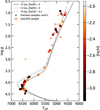Fig. 3

Kiel diagram (T_eff vs. log g): precision samples I and II, and the Gaia-ESO sample are displayed as indicated in the legends. The symbols are colour-coded according to the metallicity. Yonsey-Yale isochrones (Kim et al. 2002; Yi et al. 2003) with ages and metallicity values given in the legend are overplotted as reference.

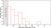Fig. 4

Histogram of isochronal ages of dwarf stars in Table A.3, binned to 0.6 Gyr, which is the median of the individual errors.

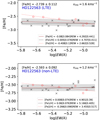Fig. 5

Ionisation equilibrium of the benchmark star HD 122563. The top and bottom panels display [Fe/H] and v_mic determination under LTE and NLTE respectively. The crosses and circles indicate neutral and ionised species, respectively. Linear regressions corresponding to each species are displayed by different line styles (see legends for, where the values in brackets are the errors of the coefficients). The red line represents the regression of the neutral and ionised species together, the shade is the 1σ standard deviation. Determined [Fe/H] and v_mic values are given in the plots.

4 Magnesium abundance

While magnesium abundances for Precision samples I and II were first derived in Giribaldi & Smiljanic (2023) and Giribaldi et al. (2023) considering generic NLTE corrections (Mashonkina 2013), we re-derived Mg abundances with updated NLTE corrections for both samples in this study and determined Mg abundances in the Gaia-ESO sample for the first time. We examined [Mg/Fe] versus [Fe/H] diagrams under different assumptions: 1D LTE, 1D NLTE, 3D LTE, and (only for dwarfs) 3D NLTE. For dwarf stars, we assumed a constant offset of +0.05 dex (in the [Mg/Fe] scale) to correct for diffusion, following the values in Table 4 of Korn et al. (2007).

The reference solar Mg abundance in all cases (1D LTE, 1D NLTE, 3D LTE, and 3D NLTE) is taken from the 3D NLTE analysis of Asplund et al. (2021), namely 7.55 ± 0.03 dex. To verify that this is consistent with our analysis, we performed line synthesis to fit a solar spectrum (light reflected in Ganymede) from the ESO archive. Using the standard parameters T_eff⊙= 5771 K (Prša et al. 2016), log g = 4.44 dex, [Fe/H] = 0 dex, and vsin i = 2.04 km s⁻¹ (dos Santos et al. 2016), we obtain A(Mg) = 7.40 and 7.50 dex from the lines at 5528 and 5711 Å, respectively; corresponding line fits are shown in Fig. A.6. The 1D LTE to 3D NLTE corrections described below for each line result in +0.11 and +0.08 dex, respectively. The 3D NLTE corrected abundances averaged over the two lines are 7.55 dex, which is compatible with the result of Asplund et al. (2021) that is based on several weaker lines of Mg I as well as of Mg II. We remark that the line 5528 Å in the solar spectrum is strong and therefore a fully solardifferential analysis with it is prone to systematic biases. On the other hand, the line at 5711 Å is only saturated with REW = −4.71, and therefore may be more suitable to that method.

4.1 1D LTE vs 1D NLTE (Turbospectrum code)

In the spectra of our three samples, Mg abundance is obtained from two lines, the Mg I lines at 5528 Å and 5711 Å. For the atomic parameters of the lines, we used the Gaia-ESO linelist (Heiter et al. 2021). In particular, the oscillator strength values (log g f ) of the two lines were from the theoretical study of Chang & Tang (1990), −0.498 and −1.724 respectively. These compare well against the values adopted by Matsuno et al. (2024), −0.547 and −1.742 (experimental and theoretical values, respectively, from Pehlivan Rhodin et al. 2017). For the 5528 Å, broadening by hydrogen collisions was described using the so called Anstee-Barklem-O’Mara (ABO) theory (Barklem & O’Mara 1997), with parameters α = 1461 and σ = 0.312. Both lines are not available in all spectra, so it is necessary to establish in which regime they give consistent A(Mg) values, so as to ensure that we always have abundances on the same scale for giant and dwarf stars.

We applied line synthesis with Turbospectrum using NLTE departure coefficients based on the model atom used in Bergemann et al. (2017). Figure 6 shows the difference between LTE and NLTE abundances retrieved from the Mg I lines at 5528 Å (top panel) and 5711 Å (bottom panel) as a function of atmospheric (A(Mg), T_eff, log g, [Fe/H]) and spectroscopic parameters (reduced equivalent widths, REW). Considering NLTE abundances as our reference, the differences displayed can be deemed as LTE biases. The maximum extent of the LTE biases of the line at 5711 Å are significantly smaller than those of line 5528 Å, as already reported in previous works (e.g. Mashonkina 2013; Bergemann et al. 2017). Namely, except for the coolest stars with lower surface gravity, its biases remain within the error bars of our determinations. For dwarf stars, LTE biases are observed to be lower than 0.04 and 0.025 dex, respectively, and therefore can be considered negligible. That is to say, 1D LTE and 1D NLTE Mg abundances of our metal-poor dwarfs are almost equivalent. These results differ from those of Andrievsky et al. (2010), where the abundances of the dwarfs are more affected than those of giants by NLTE corrections. Namely, in average, NLTE Mg of dwarfs appears larger than Mg LTE by ∼ 0.3 dex in that work.

For giants, the LTE biases of the line at 5528 Å become larger as log g and T_eff decrease. Since the absolute Mg abundance is naturally correlated with [Fe/H], the largest LTE biases remain at [Fe/H] > −2.5 dex. The bias of the line at 5528 Å responds more precisely to the REW variation, following the exponential function displayed in the plot of Fig. 6. However, the standard deviation around the exponential function increases with REW. The consistent region (REW < −4.95) has a negligible standard deviation value of 0.007 dex, whereas the saturated and over-saturated regions have a much larger standard deviation of ∼ 0.039 dex, which is comparable to the [Mg/Fe] average uncertainty of Precision Samples I and II. The plots in the figure show that out of the consistent region⁷, the LTE bias is influenced by the combination of several stellar parameters, and therefore it is more susceptible to the accuracy of all of them. Appendix B shows how the NLTE corrections of the Mg abundance evolve as A(Mg)⁸ increases. Large values are observed out of the consistent region for the line at 5528 Å, unlike for the line at 5711 Å, which remains unsaturated even for very high Mg abundances.

Most stars in our sample (37 of 55) have abundances only from the line at 5528 Å; either because the spectra do not include the weaker line at 5711 Å, or because it is not detected. We perform the following analysis to verify that our abundance scale is independent of the line choice and invariant within the parameter range of our stars. With 18 stars, we compare the consistency of the NLTE outcomes of both lines. In Figure 7 we show the abundance difference, where only error bars lower than 0.2 dex are plotted. Only the giants HD 122563 and BD+09 2870 have very precise measurements, these are indicated by the red points. Values are compatible for dwarfs and for giants with T_eff ≳ 5000 K and log g ≳ 1.8 dex.

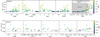Fig. 6

Comparison between 1D LTE and 1D NLTE Mg determination. Top panels: difference between 1D LTE and 1D NLTE abundance as function of atmospheric parameters, abundance, and REW for the line at 5528 Å. The rightmost panel displays an exponential function fitted to the dispersion, its coefficients are given in the plot. The shade areas cover three regions of REW: consistent (R E W<−4.95), saturated (−4.95 ≤ R E W<−4.80 ), and over-saturated ( R E W>−4.8 ) (see main text for explanation). Dispersions of the points around the fitted function are 0.0072 (consistent region), 0.0399 (saturated region), and 0.0397 dex (over-saturated region). Bottom panel: similar to the top panel, but for the line at 5511 Å.

Fig. 7

NLTE abundance differences from each line. The error bars are fitting errors related to the noise added in quadrature; only those lower than 0.2 dex are shown. The large circles indicate the parameter regions with the largest offsets. The red dots indicate the stars HD 122563 and BD+09 2870.

4.2 3D LTE versus 1D LTE (Scate code)

We used the 3D LTE code Scate (Hayek et al. 2011) to calculate 3D LTE versus 1D LTE abundance corrections for the 5528 Å line. The calculations were performed for 20 snapshots across 113 available models from the original Stagger-grid of 3D radiative-hydrodynamical model atmospheres (Magic et al. 2013); see also the updated grid of Rodríguez Díaz et al. (2024), with [Fe/H] of 0, −1, −2, and −3 dex, and spanning dwarfs and giants. The 1D calculations were performed on the 1D version of the Stagger-grid (the ATMO-grid; Appendix A of Magic et al. 2013). The 1D calculations were done with four different values of microturbulence: 0, 1, 1.5, and 2 km s⁻¹. The model atmospheres were constructed assuming the solar chemical composition of Asplund et al. (2009), scaled by [Fe/H] and with α-enhancement of +0.4 dex for the metal-poor models.

The magnesium abundance was always set to match that with which the model atmosphere was constructed. The abundance corrections were calculated by varying log g f such that the equivalent width in the 3D synthesis matched that of the 1D synthesis, for a given model atmosphere and given 1D Δ log g f . The abundance corrections are thus a function of T_eff, log g, [Fe/H], v_mic, and 1D “abundance” (as inferred from the solar-scaled and α-enhanced model atmosphere composition and Δ log g f ). These corrections were then interpolated onto the stellar parameters and 1D LTE abundance measured from the 5582 Å line.

4.3 3D NLTE versus 1D LTE (Balder code; dwarfs)

We took 3D NLTE versus 1D LTE abundance corrections for the 5582 Å from Matsuno et al. (2024). These were calculated with the code Balder (Amarsi et al. 2018), which is based on Multi3D (Leenaarts & Carlsson 2009). As with the 3D LTE abundance corrections described above, these 3D non-LTE abundance corrections are based on post-processing of the Stagger-grid of 3D radiative-hydrodynamical model atmospheres (Magic et al. 2013). The corrections are a function of T_eff, log g, v_mic, and 1D LTE abundance; the abundances of other elements were scaled with the magnesium abundance.

4.4 Determination of the uncertainties on [Mg/Fe]

The errors of A(Mg) are computed as explained in Giribaldi et al. (2023, Sect. 6.1). We briefly recall the method used. We prepared grids of 1D LTE theoretical line profiles at 5528 Å using the following parameters: for dwarfs, T_eff from 5500 to 6500 K with steps of 200 K, [Fe/H] from −1.5 to −3.0 dex with steps of 0.5 dex, log g = 4, and A(Mg) from 4.8 to 7.2 dex with steps of 0.4 dex; for giants, T_eff from 4500 to 6500 K with steps of 500 K, [Fe/H] from 1.0 to 3.0 dex with steps of 1 dex, log g from 1.0 to 3.0 dex with steps of 1 dex, and A(Mg) from 4.8 to 7.2 dex with steps of 0.4 dex. Then, we used those grids as they were observational spectra to derive Mg abundances from biased T_eff, [Fe/H], log g, and v_mic by +40 K, +0.10 dex, +0.10 dex, and +0.10 dex, respectively. This procedure gives biased A(Mg) values, whose difference with the actual A(Mg) values provides the offsets Δ(A(Mg))_param related to the parameter biases above, where param represents T_eff, log g, [Fe/H], or v_mic. The errors related to the uncertainties of the parameters in Table A.3 are obtained by multiplying the required factor. For example, if the T_eff error of the star is 80 K, Δ(A(Mg))_Teff is multiplied by 2; or if the [Fe/H] error of the star is 0.05, Δ(A(Mg))_[Fe/H] is multiplied by 0.5.

For both dwarfs and giants, the dominant source of error is due to the uncertainty in T_eff, while uncertainties in v_mic and [Fe/H] errors produce negligible Δ(A(Mg)) of the order of 0.001 dex. For dwarfs, also log g errors produce negligible Δ(A(Mg)), while it can be important for giant stars. Total A(Mg) errors are computed by adding all Δ(A(Mg))_param in quadrature, and to compute the [Mg/Fe] total error we added in quadrature those of [Fe/H] in Table A.3. The table lists the [Mg/Fe] errors in the column of 1D NLTE; however; they are also ascribed to all 1D LTE, 1D NLTE, 3D LTE and 3D NLTE determinations.

Since the temperatures are listed along with their internal errors (they do not include the uncertainty of the model 48 K), [Mg/Fe] errors of many stars are dominated by the errors of [Fe/H]. The stars with the largest [Mg/Fe] errors (e.g. those from BPS BS 16968-061 to BPS CS 29518-043) and those of the Gaia-ESO sample, own their errors to weak lines and low S/N.

5 Results

In this section, we present the results of the chemical and kinematic analysis of our sample stars, and the two chemical evolution models used to compare with them.

5.1 Compatibility of [Mg/Fe] scales between samples

The main results of our analysis are shown in Fig. 8. There, we emphasise the Gaia-Enceladus and Milky Way (MW) populations separated in Paper I as reference in background. The latter embraces the populations called Splash or heated thick disc (Belokurov et al. 2020, and references in the paper) and Erebus, which is an old (10–12 Gyr) retrograde population of low binding energy with [Fe/H] extending up to −0.5 dex. We expand on the characteristics of these populations in Sect. 5.3.

In the four panels, we show the abundances of magnesium derived with different assumptions (1D LTE, 3D LTE, 1D NLTE and 3D NLTE) in the [Mg/Fe] vsersus [Fe/H] plane; [Fe/H] is instead derived under 1D NLTE assumptions. Magnesium abundances of the Milky Way (Splash and Erebus) and Enceladus sequences in the figure were derived by means of the 1D MARCS models (Gustafsson et al. 2008) under LTE assumption. This stands for the two sub-samples from which these populations were identified: the TITANS I (Giribaldi et al. 2021) and GALAH (Buder et al. 2021), as stated in their respective papers. The Mg abundance scale of GALAH considers only the line at 5711 Å, whereas that of the TITANS I includes both lines at 5528 and 5711 Å, which, in any case, were confirmed to be equivalent, as shown in Fig. 3 of Paper I. Both the GALAH and TITANS I subsamples apply nearly identical 1D NLTE corrections. For the former, values are in between 0 and +0.05 (Fig. 7 in Amarsi et al. 2020), whereas for the latter, a constant value of +0.05 dex (Mashonkina 2013) was used. The Mg scale of the GALAH subsample was originally derived from a T_eff scale distinct to that of the TITANS I. Therefore, they were adjusted for compatibility by subtracting the relative offsets of the former, which were determined to be a constant of +0.07dex; see Sect. 5.3 of Paper I for details. Regarding the [Fe/H] scales, metallicity values of the GALAH sub-sample were not adjusted to those of the TITANS I. This is because, according to the tests in Buder et al. (2021), [Fe/H] of metal-poor GALAH stars appear to be compatible with the scale of the Gaia benchmark stars (Jofré et al. 2014); whereas the TITANS I were proven to be compatible to that scale in Giribaldi et al. (2021). Consequently, considering all the above, we can assert that the [Mg/Fe] scales of the GALAH and TITANS I subsamples from Paper I (which compose the Splash, Erebus, and Enceladus sequences in Fig. 8) are compatible and apply equivalent 1D LTE to 1D NLTE corrections.

We remark that, in Paper I, the [Mg/Fe] of the Splash, Erebus, and Enceladus populations considered a diffusion correction of +0.05 dex only for stars with [Fe/H] < −1.65 dex following the findings of Korn et al. (2007) and Gruyters et al. (2013). In line with the findings of Souto et al. (2018, 2019), we instead apply a constant diffusion correction of +0.05 dex for all dwarfs across the entire metallicity range, including the very metal-poor tail. However, see the work of Nordlander et al. (2024), which suggests that the effect of diffusion on [Mg/Fe] in stars with [Fe/H] ∼−1 dex is even closer to zero. In any case, the [Mg/Fe] sequences of the stars we compare our very metal-poor sample with are only marginally affected by these corrections.

We interpolated the 1D LTE to 3D NLTE Mg abundances of Matsuno et al. (2024), in order to obtain a 3D NLTE [Mg/Fe] scale of the Splash, Erebus, and Enceladus stars in the right bottom panel of Fig. 8. We obtain the 1D LTE scale of these stars in the top left panel by subtracting their 1D NLTE correction of 0.05. The 1D NLTE abundances in the top right panel remain as described above. Thus, we can effectively assess which chemical sequence best connects with the most metal-poor tail of the Galactic halo.

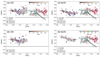Fig. 8

[Mg/Fe] vs. [Fe/H] for our sample stars: 1D LTE, 1D NLTE, 3D LTE, and 3D NLTE abundances are displayed according to the legends; all panels are built with [Fe/H] under 1D NLTE. The symbols representing the dwarfs are size-coded according to their ages. As a reference, stars classified as the in situ populations Splash (red) and Erebus (turquoise), and the ex situ population Gaia-Enceladus (grey) in Giribaldi & Smiljanic (2023) are plotted. The solid red, dashed black, and solid black lines display the LOWESS regressions. The shades display 20 to 80% quantiles. Bottom right panel: only dwarfs are displayed, as only these have 3D NLTE corrections. They are colour-coded according to age. Other panels: precision sample I (only dwarfs) has no colour-coding. The Precision sample II and Gaia-ESO sample are colour-codded according to log g. Their symbols follow the legends in the plots. The panel 1D NLTE displays the error bars of the stars in Precision samples I and II with errors larger than 0.14 dex.

5.2 The [Mg/Fe] versus [Fe/H] patterns of our samples

In each panel of Fig. 8, robust LOWESS⁹ regressions are shown along with their dispersions characterised by 20–80% quantiles. The first outcome to remark is the decrease of scatter when using NLTE corrections: at a given [Fe/H] the typical scatter in [Mg/Fe] changes from 0.07–0.27 to 0.04–0.08 dex (see shades in the plots). With 3D LTE models, the scatter remains between 0.06 and 0.12 dex, it is computed only from dwarfs; Figure A.7 shows the [Mg/Fe] dispersion variation when only dwarfs are considered. The difference between the panels on the right side in Fig. 8 lies in the possibility of applying the 3D models and NLTE corrections only to dwarf stars, i.e. to the Precision I sample and two stars of the Gaia-ESO sample. In the case of the 1D NLTE instead, abundances are calculated for both dwarf and giant stars. Using NLTE corrections (right panels), a clear sequence in the [Mg/Fe] versus [Fe/H] plane emerges for the metal-poorer population: from [Mg/Fe] + 0.6 dex for [Fe/H] < 3 dex to [Mg/Fe] ≈ + 0.4 dex for [Fe/H] ≈ 2 dex.

In the case of 1D LTE synthesis, the scatter is enhanced by the giant stars at −2.7 ≲ [Fe/H] ≲ −2 dex to high [Mg/Fe] values, which prevents distinguishing a clear pattern, as typically observed in the literature. The case of 1D NLTE displays a narrow dispersion (i.e. 0.07–0.09 dex for −2.5 < [Fe/H] < −2.0 dex), where dwarfs and giants overlap. One giant of the Gaia-ESO sample (GESJ10142785-4052503) lies far out of the sequence at about [Mg/Fe] = 0.64 dex. Its Hα profile displays a strong asymmetry, and instead we derived its T_eff by photometric relations. Therefore, we do not rule out a possible [Mg/Fe] bias arising from atmospheric parameters.

The plot with [Mg/Fe] derived in 3D NLTE contains only dwarf stars; as mentioned above, for this sample we were able to calculate ages (see histogram in Fig. 4). These are shown as a colour scale in the bottom panel on the right. As expected, the sample is composed of very old stars, with ages larger than 11 Gyr, and a median age of 12.5 Gyr. The dispersion has a similar shape to that of 1D NLTE, but it is offset upwards by +0.2 dex (see also Fig. A.7). Thus, from a purely observational point of view, we can conclude that the selected sample of old and metalpoor halo stars (see Fig. 2 for their spatial distribution) defines a somewhat tight sequence in the [Mg/Fe] versus [Fe/H] plane with a trend in [Mg/Fe] that decreases up to [Fe/H] ∼−2.8 dex, and then remains flat at [Mg/Fe] ∼ 0.4 dex for higher metallicities. This sequence becomes better defined only when NLTE corrections are properly taken into account. This could be one of the reasons why in large surveys, which generally make use of 1D LTE analysis, this portion of the [Mg/Fe] versus [Fe/H] plane looks generally more dispersed. In the next sections, we combine the chemical and kinematic properties of these stars to make some hypotheses on their origin.

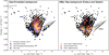Fig. 9

Lindblad diagrams (energy vs. L_Z ): the halo stars of the GALAH survey are plotted as reference background, colour-coded by density; in each panel the colour-map emphasises the Gaia-Enceladus and Milky Way (Erebus and Splash) populations, respectively, using the separation in Giribaldi & Smiljanic (2023). Left panel: precision samples and the Gaia-ESO sample (represented with the same symbols as in Fig. 2). The boxes enclose the areas with the highest probability of containing Gaia-Enceladus and Sequoia stars according to Massari et al. (2019). The red circles indicate stars with Gaia-Enceladus-like dynamics in the current sample. Right panel: stars in and out of the solar neighbourhood (distinguished by different coloured symbols). The stars with Gaia-Enceladus-like orbits are highlighted.

5.3 The kinematic properties of our samples

We computed orbital parameters using the code GalPot¹⁰ of McMillan (2017) assuming the same Galactic potential and solar kinematic parameters in Buder et al. (2021) to perform an analysis compatible with that in Paper I. Coordinates, proper motions, distances, and radial velocities are the required inputs. We use Gaia DR3 coordinates and proper motions. Radial velocities were computed from Doppler shifts, coordinates, and observation dates in the spectral files for Samples I and II; catalogued velocities were assumed for Sample III. Distances were extracted from the catalogue of Bailer-Jones (2023).

The Enceladus and the Milky Way populations (the Splash and Erebus) were identified in Paper I as follows. First, clustering was performed in the [Mg/Fe]–[Fe/H] space, considering only stars with halo-like orbits. These were identified by excluding regions occupied by the Milky Way discs in the Lindblad diagram. The distinctive knee-like shape of Enceladus, charbackground concentration in the left panel of Fig. 9). The Enceladus stars were removed from the initial sample to allow for clustering separation of the remaining stars, which exhibit a relatively high [Mg/Fe] plateau at 0.5 dex, in the Lindblad diagram. There, a prograde (Splash) and a retrograde (Erebus) populations appeared well concentrated (see the background concentration in the right panel in Fig. 9). When plotted in the [Mg/Fe]–[Fe/H] diagram, the stars of the Splash appear concentrated at high [Fe/H], whereas those of Erebus are more uniformly distributed along the [Fe/H] axis. This feature is displayed in Fig. 8, where red and turquoise circles represent each population, respectively. The age-[Fe/H] relations of these populations were observed to exhibit higher iron abundances at earlier times than Enceladus (Fig. 8 in Paper I), leading to the conclusion that both formed within a more massive galaxy and therefore likely formed in situ. These findings show that kinematic clustering alone does not definitively determine the origin of stellar populations, as seen in the simulations of Jean-Baptiste et al. (2017) and Koppelman et al. (2020).

The statistics of our very metal-poor sample is not large enough to apply machine learning algorithms for an efficient separation of different populations in kinematic diagrams (e.g. Giribaldi & Smiljanic 2023; da Silva & Smiljanic 2023; Berni 2024). Therefore, we made a visual inspection in Fig. 9. The left panel separates Precision samples I and II from the Gaia-ESO sample. The latter has several stars that seem to be associated to the bulge, as these have very high binding energy (highly negative) and are close to the Galaxy centre R_GC ≲ 5 kpc (see Fig. 2). For example, the stars with identification numbers GESJ17545552-3803393, GESJ18185545-2738118, GESJ18265160-3159404, acterised by a relatively low [Mg/Fe] plateau (at 0.25 dex), was successfully recovered. Its stars were confirmed to cluster GESJ18361733-2700053, GESJ18374490-2808311, GESJ15300154-2005148 have binding energy < −2 × 10⁵ and km s⁻² around a net L_Z of approximately zero while being widely distributed along the energy axis of the Lindblad diagram (see the and R_GC < 3.9 kpc, and so they may be the bulge members.

The right panel in Fig. 9 shows that an important fraction of the stars are positioned in correspondence with the populations of the MW, regardless if stars belong to the solar neighbourhood (blue circles) or not (grey circles). The stars BD+24 1676 (dwarf), BPS CS 22166-030 (dwarf), HD 140283 (dwarf), BPS CS 22953-003 (giant), BD+09 2870 (giant), and GESJ01293652-5020327 (giant) have Gaia-Enceladus-like orbits: nearly null rotation and high-eccentricity (stars marked in red in Fig. 9). Figure A.8 shows that these stars do not have particularly low [Mg/Fe] with respect to the trend of the sample. Also, our sample has three stars that would be candidates of belonging to the Sequoia (Barbá et al. 2019; Myeong et al. 2019) according to the selection box of Massari et al. (2019) in the Lindblad diagram (Fig. 9). As Fig. A.8 shows, neither of these stars displays low [Mg/Fe] with respect to the main trend, as expected by Matsuno et al. (2019) and Koppelman et al. (2019), for instance. These results exclude the possibility of discerning [Mg/Fe]-[Fe/H] features of populations of potential diverse origin at the range [Fe/H] ≲ 2 dex, assuming that selection by grouping into boxes in the Lindblad diagram is efficient at that. It is worth noting that Belokurov et al. (2018) already demonstrated that, within this metallicity range, stars from Gaia-Enceladus (a ∼10⁹ M_⊙ merger; e.g. Vincenzo et al. 2019; Belokurov et al. 2020) are scarce, making its kinematic imprint no longer detectable in the radial–azimuthal velocity diagram. Consequently, we consider it most viable to regard the stars in this metallicity range as having formed either in the early Milky Way – by then already the dominant mass contributor of the Local Group alongside M 31 – or in smaller progenitor galaxies of comparable stellar mass, which were later assimilated (e.g. Malhan & Rix 2024). Given their similar age and metallicity, distinguishing between the two scenarios remains challenging, as no quantitative evidence currently favours one over the other.

5.4 Chemical evolution models

To interpret the chemical properties of our metal-poor star sample (see Sect. 5.2), we applied two distinct chemical evolution models: one specifically tailored for Boötes I, one of the most extensively studied ultra-faint dwarf (UFD) galaxies both observationally and theoretically (see e.g. Koch et al. 2009; Lai et al. 2011), and a Galactic Chemical Evolution (GCE) model (Romano et al. 2017, 2019; Rossi et al. 2024a) that traces the composition of stars formed in situ in the Milky Way.

By comparing the data with the predictions of these two models, we aim to analyse the differences between accreted stars (i.e. stars born in UFD progenitors), and stars born in situ, thereby shedding light in a quantitative way on the origin of the population under study.

5.4.1 Ultra-faint dwarf model

The model has been extensively described in a series of papers (Rossi et al. 2021, 2023, 2024b), to which we refer for further details. Here, we present a brief summary of the main assumptions underlying the model. The model tracks the formation and evolution of a Boötes I-like galaxy from the epoch of its formation until redshift z = 0. It assumes that the UFD galaxy evolves in isolation, without undergoing major merger events, in line with cosmological models (Salvadori & Ferrara 2009; Salvadori et al. 2015). At the epoch of virialisation, the total amount of gas is assumed to have a pristine chemical composition. Star formation becomes possible when the gas begins to fall into the central region of the halo and cools down (Rossi et al. 2021). The total mass of stars formed within a timescale of 1 Myr is evaluated by assuming a star formation rate, Ψ, regulated by the free-fall time (t_ff) and the mass of cold gas accreted via infall (M_cold): Ψ = ϵ_⋆M_cold/t_ff, where ϵ_⋆ is a free parameter of the model. No specific assumption regarding the star formation history is made.

The model assumes that according to the metallicity of the interstellar medium (ISM) Population III (Pop III) or Population II/I (Pop II/I) stars can form. Following the critical metallicity scenario (Bromm et al. 2001; Schneider et al. 2003; Omukai et al. 2005), Pop III stars form only if the metallicity of the gas¹¹, Z_gas, is below a critical threshold, Z_cr = 10^−4.5±1Z_⊙ (i.e. when Z_gas ≤Z_cr). Once Z_gas exceeds this threshold, Pop II/I stars begin to form. The newly formed stellar mass is distributed according to the Initial Mass Function (IMF) of Larson (1981), with a characteristic mass of m_ch = 10 M_⊙ for Pop III stars and m_ch = 0.35 M_⊙ for Pop II/I stars, within the mass ranges 0.8–1000 M_⊙ and 0.1–100 M_⊙ , respectively.

The model accounts for the incomplete sampling of the stellar IMF for both Pop III and Pop II stellar populations. Each time the conditions for star formation are reached, a discrete number of stars is formed, with their masses randomly drawn from the specified IMF. This feature is crucial for accurately simulating the evolution of UFDs with low star formation rates, where the IMF is never fully sampled over the galaxy’s lifetime (see Rossi et al. 2021). The chemical enrichment of the gas is tracked by considering the mass-dependent evolutionary timescales of individual stars. Specifically, the semi-analytical model follows the release of chemical elements (from carbon to zinc) by supernovae (SNe) and AGB stars. The contribution of supernovae Type Ia (SNIa) has been included adopting the yields of Iwamoto et al. (1999) and the bimodal delay time distribution observationally derived by Mannucci et al. (2006). Ad each time-step the rate of SNIa is computed following the prescriptions of Matteucci et al. (2006).

For Pop III SNe in the mass range 10–100 M , we adopt the stellar yields of Heger & Woosley (2010), while for Pair Instability SNe (PISN) in the mass range m_PISN = 140–260 M we use the ones of Heger & Woosley (2002). For less massive Pop III stars in the mass range 2–8 M_⊙ we account for the AGB yields of Meynet & Maeder (2002) (rotating model). For Pop II/I stars, we employed stellar yields dependent on the initial mass and metallicity of the stars. Specifically, for Pop II/I SNe arising from progenitors in the mass range 8–40 M_⊙ we employed the stellar yields of Limongi & Chieffi (2018), their set R, which assumes no rotation, while for AGB stars the ones of van den Hoek & Groenewegen (1997). The mechanical feedback from SNe is accounted. Indeed, SNe explosions can produce blast waves that, if sufficiently energetic, are capable of overcoming the gravitational potential of the host halo, leading to the ejection of gas and metals into the intergalactic medium (IGM). The ejected mass, M_ej, is given by: $M_{ej} = \frac{2 ϵ_{w} N_{SN} E_{SN}}{v_{sc}^{2}}$ $\frame{\frame{\text{M}}_\frame{\frame{\text{ej}}}} = \frac{\frame{2\frame{\varepsilon _\frame{\text{w}}}\frame{\frame{\text{N}}_\frame{\frame{\text{SN}}}}\frame{\frame{\text{E}}_\frame{\frame{\text{SN}}}}}}{\frame{\frame{\text{v}}_\frame{\frame{\text{sc}}}^2}}$ , where ϵ_w is the efficiency of the SNe-driven winds and it is a free parameter of the model, N_SN is the number of SNe, E_SN is the explosion energy, and v_esc is the escape velocity of the halo, which depends on its mass, M_h, and virial radius. The ejected gas fully mixes with the ISM, ensuring its metallicity matches that of the ISM. The free parameters (ϵ_⋆, ϵ_w) have been fixed to reproduce the observed properties of Boötes I UFD (its total luminosity, star formation history, metallicity distribution function, and average stellar iron abundance; see e.g. Brown et al. 2014; Simon 2019; Jenkins et al. 2021), here taken as representative of the prototype UFD that interacted and merged with the Milky Way in its earlier evolutionary phases.

5.4.2 Galactic chemical evolution model

To simulate the chemical enrichment of stellar populations that formed in situ in the early Milky Way (see e.g. Belokurov & Kravtsov 2022) we use a comprehensive GCE model fully described in Romano et al. (2017, 2019, 2020) and Rossi et al. (2024a). The model incorporates both homogeneous and stochastic enrichment processes and integrates contributions from Pop III stars, which play a pivotal role in the early phases of the Galaxy’s chemical evolution (see Rossi et al. 2024a). The GCE model is constructed with a multizone approach, segmenting the Galactic disc into concentric annuli of 2 kpc width each. This allows us to account for radial variations in star formation, gas inflow, and enrichment processes across the disc. For the comparison with the data sample analysed in this paper, we consider the model predictions relevant to an annulus centred on the Sun’s position (R_GC = 7–9 kpc). The model assumes an initial accretion phase of primordial material, which serves as the foundation for the formation of the in situ halo and thickdisc components. During this early phase (lasting 3–4 Gyr, see Spitoni et al. 2019, 2021), the rapid gas accretion triggers an intense star formation activity, depleting the initial gas reservoir and producing the most ancient stellar populations. A second, prolonged accretion event leads to the formation of the thin disc, characterised by an inside-out growth pattern where the inner regions evolve more rapidly than the outer ones (Romano et al. 2000; Chiappini et al. 2001). The star formation rate is governed by the Schmidt-Kennicutt law (Kennicutt 1998), with a surface density power-law index of 1.5 and a radially dependent star formation efficiency to reproduce the observed gradients in the present-day MW disc (see e.g. Palla et al. 2020). The newly formed stellar mass is distributed in the mass range 0.1– 100 M according to the field IMF of Kroupa et al. (1993). To follow the chemical enrichment, the model tracks the contributions from H to Eu from stars of different masses and lifetimes. The chemical enrichment from low- and intermediate-mass stars (LIMS; 1–6 M ) is modelled using non-rotating yields provided in the FRUITY database (Cristallo et al. 2009, 2011, 2015), which successfully reproduces MW abundances across various components (Molero et al. 2023, Romano et al., in prep). For massive stars (13–120 M ), exploding as core-collapse supernovae (CCSNe), we use the yields of Limongi & Chieffi (2018) (set R and rotating models with velocity 150 km/s). For SNe Type Ia, we adopt the yields of Iwamoto et al. (1999), which are critical for reproducing the [α/Fe] decline at higher metallicities. The model also includes novae that became important after 1 Gyr from the beginning of star formation, due to the time delay associated with their binary nature (Romano et al. 1999, and references therein). To address the inhomogeneous enrichment characteristic of the MW’s early phases, we incorporate a stochastic star formation component. In this scheme, initial gas clumps form stars under conditions that mimic the localised, self-enriching star-forming regions that later merge into the Galactic halo. Each clump hosts a Pop III star of randomly chosen mass (10–100 M_⊙ ) and explosion energy, selected from the grid of models computed by Heger & Woosley (2010). The wide range of SNe yields for Pop III stars, together with clump-specific dilution factors, explains the significant scatter of abundances observed in MW halo stars (see Rossi et al. 2024a, for further details). In particular, the model is calibrated against CNO abundance data of metal-poor MW stars from recent spectroscopic surveys (Mucciarelli et al. 2022; Amarsi et al. 2019).

6 Discussion

By applying 1D NLTE and 3D NLTE spectral synthesis, we have demonstrated that at least part of the large [Mg/Fe] dispersion at the metal poorest tail (−3.5 ≲ [Fe/H] ≲ −2 dex), typically observed in the literature, is due to the application of the LTE assumption on giant stars. As shown in the right panels in Fig. 8, our observational data composed of dwarfs and giants support a narrow [Mg/Fe] distribution, as previously proposed by Arnone et al. (2005) and Andrievsky et al. (2010), for instance. Therefore, it indicates a low degree of stochastic enrichment 12.5 Gyr ago, which is the median age of our sample. At the same time, a mildly decreasing trend with metallicity is observed, from [Mg/Fe] ≃0.65 at [Fe/H] ≃ −3.3 to [Mg/Fe] ≃ 0.4 at [Fe/H] ≃ −2.0.

We show that the sequence of the metal-poorest tail is compatible with that of the Milky Way (i.e. they join at [Mg/Fe] ≈0.4 dex) only when 3D NLTE is applied (bottom right panel in Fig. 8), whereas 1D NLTE (and other assumptions) switch [Mg/Fe] down by ∼0.2 dex misleading continuity with the Gaia-Enceladus sequence.

By comparing the 3D NLTE chemical trend with the predictions of inhomogeneous chemical evolution models that trace the chemical properties of stars formed in situ in the early MW and in a prototype UFD progenitor, taken as an example of a lowmass galaxy like the ones accreted by the Milky Way, we can try to place constraints on the origin of our metal-poor population. In Fig. 10, the predictions of the chemical evolution models for the early Milky Way (in situ component only) and the UFD galaxy Boötes I are shown in the [Mg/Fe] versus [Fe/H] plane. The density maps represent stellar distributions predicted by the model. Individual data points correspond to our high-precision measurements (3D NLTE abundances, shown also in the bottom left of Fig. 8) allowing for a comparison between model predictions and observed abundances.

The two density maps highlight distinct enrichment patterns for the early MW and Boötes I. The Milky Way halo/early disc follows a more complex evolutionary path, with efficient and continuous star formation driving a rapid iron enrichment and a steady decline in [Mg/Fe] as [Fe/H] increases. In contrast, Boötes I exhibits a simpler evolutionary path, marked by low star formation rates and more intermittent star formation episodes, shaped by stronger feedback effects and substantial mass loss (see Rossi et al. 2024b). The flat trend and the large scatter in [Mg/Fe] versus [Fe/H] is largely due to the initial enrichment dominated by Pop III stars, which contribute substantial magnesium in the early evolutionary phases. The Milky Way undergoes a more extended period of star formation, increasingly dominated by Pop II stars, whose iron enrichment gradually reduces the initial chemical impact of the Pop III contribution as the metallicity increases. Both models display some scatter in [Mg/Fe] due to stochastic processes and low star formation rate in the earliest phases of their evolution, although areas of higher stellar density show more marked trends. In particular, in the model of the UDF, the regions of highest density, therefore most likely, are those with a high [Mg/Fe]. There is a good agreement -especially if a small offset is applied to the theoretical [Mg/Fe] ratiowith the values of [Mg/Fe] in our sample for [Fe/H] around −2.5 dex, while stars at lower [Fe/H] with high [Mg/Fe] are less likely predicted in the UDF model. This might support the idea that some of the stars analysed in this work once belonged to dwarf galaxies. However, to confirm or not this result, other elements are needed to discriminate between in situ and accreted origins; for instance, Zn could provide interesting hints¹² (see e.g. Mucciarelli et al. 2021).

Our sample could be composed of in situ stars, as the comparison reveals an overall consistency with the tail at high [Mg/Fe] for very metal-poor stars in the MW model, once a positive offset is considered (as shown in the figure). This offset is indeed required due to the well-known problem of Mg under-production in stellar evolution and nucleosynthesis models, which leads to discrepancies between GCE model predictions and observations that are particularly pronounced at disc metallicities (see e.g. Timmes et al. 1995; Romano et al. 2010; Prantzos et al. 2018; Kobayashi et al. 2020). This sometimes prompted the usage of empirical yields to better fit the observations (e.g. François et al. 2004; Spitoni et al. 2019, 2021). Here we deal with early inhomogeneous chemical enrichment utilising different sets of yields/dilution factors (see Rossi et al. 2024a) and do not apply any correction to the yields. However, we note that higher Mg yields from Pop II stars would bring the highdensity regions of the stellar maps shown in Fig. 10 in better agreement with the loci occupied by the data. This is particularly true for the MW model, which is dominated by the contribution of Pop II stars. To guide the eye, a positive offset of +0.4 dex is shown (dashed line in both panels). The trends in both the GCE and UDF models might provide both a plausible explanation for the origin of stars with [Fe/H] < –2.8 dex and high [Mg/Fe].

Moreover, beyond chemical evolution models, it is also important to consider dynamical information to better constrain the origin of our sample stars. As shown in the Lindblad diagram of Fig. 9, most of the stars in our sample have orbital parameters consistent with those of halo populations, like Gaia-Enceladus (accreted), Erebus or Splash (both in situ). Most importantly, from a dynamical perspective, our sample lacks coherence, as would be instead expected for stars originating from a common progenitor galaxy, particularly if the merger occurred relatively recently (see e.g. Helmi & de Zeeuw 2000). However, clumps in dynamical spaces are typically neither complete nor pure (JeanBaptiste et al. 2017). For instance, numerical models of galaxy interactions by Mori et al. (2024) suggest that in high-mass mergers (mass ratios of ∼1:10), the stars of the accreted galaxy can more efficiently lose coherence in the E-Lz plane, whereas this is less likely for lower-mass mergers (Amarante et al. 2022; Khoperskov et al. 2023). Additionally, recent models of the hierarchical assembly of galaxy halos indicate that stars accreted from progenitor fragments can be identified through their chemical signatures, enabling the distinction between in situ, ex situ, and endo-debris populations (Gonzalez-Jara et al. 2025), but can be less evident in the kinematic space.

Therefore, when analyzing stars like those in our sample, which are inhomogeneously distributed in dynamical space, a common origin cannot be definitively ruled out. At present, using only Mg and Fe, we are unable to discern subtle differences that could reveal their chemical origin. However, a more extensive analysis incorporating additional elements, carefully examined in 3D NLTE, may provide the necessary insights to disentangle their origin.

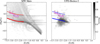Fig. 10

Predicted [Mg/Fe] versus [Fe/H] density maps. Left panel: chemical evolution model for the Milky Way. Right panel: chemical evolution model for UFD galaxy Boötes I, taken as a prototype of the satellites accreted by the MW at early times. The highest density region of the GCE model and the average of UDF model are offset by +0.4 dex (dotted red line and dotted blue line, respectively) to allow a better comparison with the observed abundances. The pink solid line is the LOWESS regression. The circles represent the Precision I sample with Mg under 3D NLTE.

7 Summary and conclusions

Given the current understanding that orbital properties alone are likely insufficient to determine the membership of halo stars to a debris field or a disrupted satellite in the inner halo (R_GC < 30 kpc) (e.g. Horta et al. 2023; Gonzalez-Jara et al. 2025), we conducted a high-precision spectral analysis of low-metallicity halo stars to obtain optimal chemical abundances. Our results reveal a remarkably tight sequence in [Mg/Fe] versus [Fe/H], suggesting a shared chemical evolutionary pathway for our sample. This sequence likely traces the primordial halo, particularly at very early epochs with low metallicity, as its knee-like shape closely aligns with predictions from our GCE model. Alternatively, the observed sequence may also be compatible with UFD models, characterised by low star formation efficiency. Both models require an empirical shift of +0.4 dex at most to match both the observational data and the solar [Mg/Fe] = 0 constraint. The combination of chemical homogeneity and kinematic incoherence complicates the unambiguous identification of these stars’ origins, making them consistent with both the early evolution of the Milky Way halo and that of UFDs. Additionally, the tightness of the sequence suggests that stochastic enrichment, at least for Mg, is not highly dominant in the metallicity range of our sample, as it is significantly more constrained than model predictions. Increasing the sample of metal-poor stars, and the analysis of elements such as Al and Na, for example, with the kind of NLTE analysis presented here will better reveal if they originated in a common progenitor. This is indeed one of the drivers of forthcoming projects for new instrumentation, such as HRMOS (Magrini et al. 2023) and WST (Mainieri et al. 2024).

Acknowledgements

R.E.G. and L.M. thank INAF for the support (Large Grant 2023 EPOCH) and for the MiniGrant 2022 Checs. They acknowledge financial support under the National Recovery and Resilience Plan (NRRP), Mission 4, Component 2, Investment 1.1, Call for tender No. 104 published on 2.2.2022 by the Italian Ministry of University and Research (MUR), funded by the European Union – NextGenerationEU– Project ‘Cosmic POT’ (PI: L. Magrini) Grant Assignment Decree No. 2022X4TM3H by the Italian Ministry of Ministry of University and Research (MUR). DR and MR research is supported by INAF (Theory Grant 2022, “An in-depth theoretical study of CNO element evolution in galaxies”, Fu. Ob. 1.05.12.06.08). D.M. research is funded by the European Union –NextGenerationEU” RRF M4C2 1.1 n: 2022HY2NSX. “CHRONOS: adjusting the clock(s) to unveil the CHRONO-chemo-dynamical Structure of the Galaxy” (PI: S. Cassisi) AMA gratefully acknowledges support from the Swedish Research Council (VR 2020-03940) and from the Crafoord Foundation via the Royal Swedish Academy of Sciences (CR 2024-0015). Use was made of the Simbad database, operated at the CDS, Strasbourg, France, and of NASA’s Astrophysics Data System Bibliographic Services. This publication makes use of data products from the Two Micron All Sky Survey, which is a joint project of the University of Massachusetts and the Infrared Processing and Analysis Center/California Institute of Technology, funded by the National Aeronautics and Space Administration and the National Science Foundation. This research used Astropy (http://www.astropy.org) a community-developed core Python package for Astronomy (Astropy Collaboration 2018). This work presents results from the European Space Agency (ESA) space mission Gaia. Gaia data are processed by the Gaia Data Processing and Analysis Consortium (DPAC). Funding for the DPAC is provided by national institutions, in particular the institutions participating in the Gaia MultiLateral Agreement (MLA). The Gaia mission website is https://www.cosmos.esa.int/gaia. The Gaia archive website is https://archives.esac.esa.int/gaia.

Appendix A Additional figures and tables

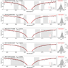Fig. A.1

Hα profile fits of five dwarf stars from Meléndez et al. (2010). In the left panels the observational spectra are shown in black. The fitted 3D NLTE synthetic Hα line profile is represented by the red continuous line, and a synthetic profile related to a T_eff −200 K is represented by the dashed red line. Shades represent the windows of fits employed. The right panels show histograms of the temperature values related every pixel within the windows of the fits. The histograms are fitted by Gaussian distributions (black lines), whose medians and 1σ dispersions, are the most likely T_eff values and their corresponding errors.

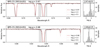Fig. A.2

Magnesium profile fits of the star BPS CS 29518−051. The observational profile is represented in black. The red lines represent synthetic profiles. The thick line corresponds to the lost likely log g. The right panels show histograms of the log g values associated with all the pixels within the shaded windows. The most probable log g and its error are obtained by bootstrapping.

Fig. A.3

Probable flux emission at the red wing of the Hα profile of the star GESJ81855445-2738118. The elements of the plot are the same as those in Fig. A.1. The red wing is more compatible with a cool profile (dashed red line), whereas the blue wing is deeper, and therefore hotter, than the hot profile (continuum red line).

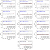Fig. A.4

Determination of metallicity and microturbulence of stars of Precision sample II. The abundances of Fe I lines are represented by cross symbols, whereas those of Fe II are represented by red circles. Regressions of each species are represented by the black dotted and red dotted lines, respectively. The red line represents the regression of both Fe I and Fe II species together. The shade represents 1σ dispersion. Regressions are computed considering 2σ clipping.

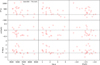Fig. A.5

Comparison of atmospheric parameters.

The horizontal axis displays the parameters determined in this work.

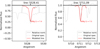Fig. A.6

Mg line fits in the solar spectrum reflected in Ganymede. The dashed line represents the observed spectrum normalised by our automatic pipeline. It shows obvious flux mislocation with respect to the unity. The continuous black line displays the spectrum re-normalised on the fly by our line-fitting algorithm, which uses the pseudo-continuum of the synthetic spectrum (red line) as the flux reference. Abundances recovered by fitting are noted in the plots.

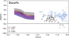Fig. A.7

LOWESS dispersions of [Mg/Fe] of dwarfs.

Shades of different colours display 1D LTE, 3D LTE, 1D NLTE, and 3D NLTE assumptions according to the legends. As in Fig. 8, the Milky Way and Enceladus populations are plotted in blue and grey as reference.

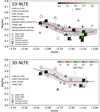Fig. A.8

Close up of the 1D NLTE and 3D NLTE [Mg/Fe] versus [Fe/H] diagram. The plots display the same as right column panels in Fig. 8. The numbers indicate the stars that show Enceladus-like orbits (green numbers) and Sequoia-like orbits (red numbers) in Fig. 9.

Table A.1

Iron line list.

Table A.2

Effective temperature determinations from diverse methods, spectral resolution and signal-to-noise ratio.

Table A.3

Stellar parameters of the stars

Appendix B Curve of growth of the Mg line at 5528 Å

Figure B.1 shows the theoretical curve of growth of both Mg lines for BD+09 2870, a cool (T_eff = 4724 K) and relatively lowgravity (log g = 1.4) star in the over-saturated region of the plot. Thick lines represent 1D LTE and the thin lines represent 1D NLTE. Both lines are colour-coded by the slope δREW/δA(Mg). The NLTE curve of the line 5528 Å bifurcates from that of LTE as A(Mg) and REW increase, predicting progressively lower A(Mg) determinations. The difference between 1D LTE and 1D NLTE is larger in the saturated and over-saturated regions of the curve because the slope approximates to zero. For instance, the REW = −4.76 of the 5528 Å line of the star corresponds to [Mg/Fe] values of 0.30 and 0.65 dex in the 1D NLTE and 1D LTE curves, respectively (see crosses in the plot). On the other hand, the curves of growth of the line at 5711 Å do not get as saturated as those of 5528 Å, even for extremely high abundances such as [Mg/Fe] ≳ 0.8 dex. Additionally, LTE and NLTE curves are almost superimposed, with a constant separation of REW+0.02 or [Mg/Fe] −0.04 of the latter with respect to the former.

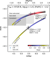Fig. B.1

Theoretical curves of growth of the Mg lines at 5528 and 5711 Å. The curves correspond to the star BD+09 2870, the parameters of which are given in the plot. The thick and thin lines represent NLTE and LTE, respectively. The NLTE curve of the line at 5711 Å is marked by the dashed line. The crosses symbols indicate REW and corresponding Mg abundances in LTE and NLTE for each line; values are noted in the plot.

References

Abdurro’uf Accetta, K., Aerts, C., et al. 2022, ApJS, 259, 35 [NASA ADS] [CrossRef] [Google Scholar]
Aguado, D. S., González Hernández, J. I., Allende Prieto, C., & Rebolo, R. 2019, ApJ, 874, L21 [NASA ADS] [CrossRef] [Google Scholar]
Aguado, D. S., Molaro, P., Caffau, E., et al. 2022, A&A, 668, A86 [NASA ADS] [CrossRef] [EDP Sciences] [Google Scholar]
Allard, N. F., Kielkopf, J. F., Cayrel, R., & van’t Veer-Menneret, C. 2008, A&A, 480, 581 [NASA ADS] [CrossRef] [EDP Sciences] [Google Scholar]
Amarante, J. A. S., Debattista, V. P., Beraldo e Silva, L., Laporte, C. F. P., & Deg, N. 2022, ApJ, 937, 12 [NASA ADS] [CrossRef] [Google Scholar]
Amarsi, A. M., Nordlander, T., Barklem, P. S., et al. 2018, A&A, 615, A139 [NASA ADS] [CrossRef] [EDP Sciences] [Google Scholar]
Amarsi, A. M., Nissen, P. E., Asplund, M., Lind, K., & Barklem, P. S. 2019, A&A, 622, L4 [NASA ADS] [CrossRef] [EDP Sciences] [Google Scholar]
Amarsi, A. M., Lind, K., Osorio, Y., et al. 2020, A&A, 642, A62 [EDP Sciences] [Google Scholar]
Andrievsky, S. M., Spite, M., Korotin, S. A., et al. 2010, A&A, 509, A88 [NASA ADS] [CrossRef] [EDP Sciences] [Google Scholar]
Aoki, W., Frebel, A., Christlieb, N., et al. 2006, ApJ, 639, 897 [Google Scholar]
Aoki, W., Beers, T. C., Lee, Y. S., et al. 2013, AJ, 145, 13 [CrossRef] [Google Scholar]
Arentsen, A., Aguado, D. S., Sestito, F., et al. 2023, MNRAS, 519, 5554 [NASA ADS] [CrossRef] [Google Scholar]
Arnone, E., Ryan, S. G., Argast, D., Norris, J. E., & Beers, T. C. 2005, A&A, 430, 507 [NASA ADS] [CrossRef] [EDP Sciences] [Google Scholar]
Asplund, M., Grevesse, N., Sauval, A. J., & Scott, P. 2009, ARA&A, 47, 481 [NASA ADS] [CrossRef] [Google Scholar]
Asplund, M., Amarsi, A. M., & Grevesse, N. 2021, A&A, 653, A141 [NASA ADS] [CrossRef] [EDP Sciences] [Google Scholar]
Astropy Collaboration (Price-Whelan, A. M., et al.) 2018, AJ, 156, 123 [Google Scholar]
Ayrton, B. 2021, https://github.com/AyrtonB/Merit-Order-Effect [Google Scholar]
Bailer-Jones, C. A. L. 2023, AJ, 166, 269 [NASA ADS] [CrossRef] [Google Scholar]
Baratella, M., D’Orazi, V., Carraro, G., et al. 2020, A&A, 634, A34 [NASA ADS] [CrossRef] [EDP Sciences] [Google Scholar]
Baratella, M., D’Orazi, V., Sheminova, V., et al. 2021, A&A, 653, A67 [NASA ADS] [CrossRef] [EDP Sciences] [Google Scholar]
Barbá, R. H., Minniti, D., Geisler, D., et al. 2019, ApJ, 870, L24 [CrossRef] [Google Scholar]
Barklem, P. S. 2007, A&A, 466, 327 [NASA ADS] [CrossRef] [EDP Sciences] [Google Scholar]
Barklem, P. S., & O’Mara, B. J. 1997, MNRAS, 290, 102 [Google Scholar]
Barklem, P. S., Piskunov, N., & O’Mara, B. J. 2000, A&A, 363, 1091 [NASA ADS] [Google Scholar]
Barklem, P. S., Stempels, H. C., Allende Prieto, C., et al. 2002, A&A, 385, 951 [NASA ADS] [CrossRef] [EDP Sciences] [Google Scholar]
Belokurov, V., & Kravtsov, A. 2022, MNRAS, 514, 689 [NASA ADS] [CrossRef] [Google Scholar]
Belokurov, V., Erkal, D., Evans, N. W., Koposov, S. E., & Deason, A. J. 2018, MNRAS, 478, 611 [Google Scholar]
Belokurov, V., Sanders, J. L., Fattahi, A., et al. 2020, MNRAS, 494, 3880 [Google Scholar]
Bergemann, M., Lind, K., Collet, R., Magic, Z., & Asplund, M. 2012, MNRAS, 427, 27 [Google Scholar]
Bergemann, M., Collet, R., Amarsi, A. M., et al. 2017, ApJ, 847, 15 [NASA ADS] [CrossRef] [Google Scholar]
Berni, L. 2024, arXiv e-prints [arXiv:2409.11429] [Google Scholar]
Bonaca, A., Conroy, C., Cargile, P. A., et al. 2020, ApJ, 897, L18 [NASA ADS] [CrossRef] [Google Scholar]
Borre, C. C., Aguirre Børsen-Koch, V., Helmi, A., et al. 2022, MNRAS, 514, 2527 [NASA ADS] [CrossRef] [Google Scholar]
Bromm, V., Ferrara, A., Coppi, P., & Larson, R. 2001, MNRAS, 328, 969 [NASA ADS] [CrossRef] [Google Scholar]
Brook, C. B., Kawata, D., Gibson, B. K., & Flynn, C. 2003, ApJ, 585, L125 [NASA ADS] [CrossRef] [Google Scholar]
Brown, T. M., Tumlinson, J., Geha, M., et al. 2014, ApJ, 796, 91 [NASA ADS] [CrossRef] [Google Scholar]
Buder, S., Sharma, S., Kos, J., et al. 2021, MNRAS, 506, 150 [NASA ADS] [CrossRef] [Google Scholar]
Caffau, E., Bonifacio, P., François, P., et al. 2012, A&A, 542, A51 [NASA ADS] [CrossRef] [EDP Sciences] [Google Scholar]
Casagrande, L., Ramírez, I., Meléndez, J., Bessell, M., & Asplund, M. 2010, A&A, 512, A54 [NASA ADS] [CrossRef] [EDP Sciences] [Google Scholar]
Casagrande, L., Portinari, L., Glass, I. S., et al. 2014, MNRAS, 439, 2060 [Google Scholar]
Casagrande, L., Lin, J., Rains, A. D., et al. 2021, MNRAS, 507, 2684 [NASA ADS] [CrossRef] [Google Scholar]
Cayrel, R., Depagne, E., Spite, M., et al. 2004, A&A, 416, 1117 [NASA ADS] [CrossRef] [EDP Sciences] [Google Scholar]
Ceccarelli, E., Massari, D., Mucciarelli, A., et al. 2024, A&A, 684, A37 [NASA ADS] [CrossRef] [EDP Sciences] [Google Scholar]
Cescutti, G., Bonifacio, P., Caffau, E., et al. 2022, A&A, 668, A168 [NASA ADS] [CrossRef] [EDP Sciences] [Google Scholar]
Chang, T. N., & Tang, X. 1990, J. Quant. Spec. Radiat. Transf., 43, 207 [Google Scholar]
Chiappini, C., Matteucci, F., & Romano, D. 2001, ApJ, 554, 1044 [NASA ADS] [CrossRef] [Google Scholar]
Christlieb, N., Bessell, M. S., Beers, T. C., et al. 2002, Nature, 419, 904 [NASA ADS] [CrossRef] [PubMed] [Google Scholar]
Cohen, J. G., Christlieb, N., Thompson, I., et al. 2013, ApJ, 778, 56 [Google Scholar]
Cristallo, S., Straniero, O., Gallino, R., et al. 2009, ApJ, 696, 797 [NASA ADS] [CrossRef] [Google Scholar]
Cristallo, S., Piersanti, L., Straniero, O., et al. 2011, ApJS, 197, 17 [NASA ADS] [CrossRef] [Google Scholar]
Cristallo, S., Straniero, O., Piersanti, L., & Gobrecht, D. 2015, ApJS, 219, 40 [Google Scholar]
da Silva, A. R., & Smiljanic, R. 2023, A&A, 677, A74 [NASA ADS] [CrossRef] [EDP Sciences] [Google Scholar]
Dekker, H., D’Odorico, S., Kaufer, A., Delabre, B., & Kotzlowski, H. 2000, SPIE Conf. Ser., 4008, 534 [NASA ADS] [Google Scholar]
De Silva, G. M., Freeman, K. C., Bland-Hawthorn, J., et al. 2015, MNRAS, 449, 2604 [NASA ADS] [CrossRef] [Google Scholar]
dos Santos, L. A., Meléndez, J., do Nascimento, J.-D., et al. 2016, A&A, 592, A156 [NASA ADS] [CrossRef] [EDP Sciences] [Google Scholar]
Dutra-Ferreira, L., Pasquini, L., Smiljanic, R., Porto de Mello, G. F., & Steffen, M. 2016, A&A, 585, A75 [NASA ADS] [CrossRef] [EDP Sciences] [Google Scholar]
Eggen, O. J., Lynden-Bell, D., & Sandage, A. R. 1962, ApJ, 136, 748 [NASA ADS] [CrossRef] [Google Scholar]
Feuillet, D. K., Sahlholdt, C. L., Feltzing, S., & Casagrande, L. 2021, MNRAS, 508, 1489 [NASA ADS] [CrossRef] [Google Scholar]
François, P., Matteucci, F., Cayrel, R., et al. 2004, A&A, 421, 613 [NASA ADS] [CrossRef] [EDP Sciences] [Google Scholar]
François, P., Depagne, E., Hill, V., et al. 2007, A&A, 476, 935 [Google Scholar]
François, P., Cescutti, G., Bonifacio, P., et al. 2024, A&A, 686, A295 [NASA ADS] [CrossRef] [EDP Sciences] [Google Scholar]
Frebel, A., Aoki, W., Christlieb, N., et al. 2005, Nature, 434, 871 [CrossRef] [Google Scholar]
Gallart, C., Bernard, E. J., Brook, C. B., et al. 2019, Nat. Astron., 3, 932 [Google Scholar]
Gerber, J. M., Magg, E., Plez, B., et al. 2023, A&A, 669, A43 [NASA ADS] [CrossRef] [EDP Sciences] [Google Scholar]
Gilmore, G., Randich, S., Worley, C. C., et al. 2022, A&A, 666, A120 [NASA ADS] [CrossRef] [EDP Sciences] [Google Scholar]
Giribaldi, R. E., & Smiljanic, R. 2023, A&A, 673, A18 [NASA ADS] [CrossRef] [EDP Sciences] [Google Scholar]
Giribaldi, R. E., Ubaldo-Melo, M. L., Porto de Mello, G. F., et al. 2019, A&A, 624, A10 [NASA ADS] [CrossRef] [EDP Sciences] [Google Scholar]
Giribaldi, R. E., da Silva, A. R., Smiljanic, R., & Cornejo Espinoza, D. 2021, A&A, 650, A194 [NASA ADS] [CrossRef] [EDP Sciences] [Google Scholar]
Giribaldi, R. E., Van Eck, S., Merle, T., et al. 2023, A&A, 679, A110 [NASA ADS] [CrossRef] [EDP Sciences] [Google Scholar]
Gonzalez-Jara, J., Tissera, P. B., Monachesi, A., et al. 2025, A&A, 693, A282 [NASA ADS] [CrossRef] [EDP Sciences] [Google Scholar]
Grand, R. J. J., Kawata, D., Belokurov, V., et al. 2020, MNRAS, 497, 1603 [NASA ADS] [CrossRef] [Google Scholar]
Gruyters, P., Korn, A. J., Richard, O., et al. 2013, A&A, 555, A31 [NASA ADS] [CrossRef] [EDP Sciences] [Google Scholar]
Gustafsson, B., Edvardsson, B., Eriksson, K., et al. 2008, A&A, 486, 951 [NASA ADS] [CrossRef] [EDP Sciences] [Google Scholar]
Hansen, C. J., Bergemann, M., Cescutti, G., et al. 2013, A&A, 551, A57 [NASA ADS] [CrossRef] [EDP Sciences] [Google Scholar]
Hayek, W., Asplund, M., Collet, R., & Nordlund, Å. 2011, A&A, 529, A158 [NASA ADS] [CrossRef] [EDP Sciences] [Google Scholar]
Heger, A., & Woosley, S. E. 2002, ApJ, 567, 532 [Google Scholar]
Heger, A., & Woosley, S. E. 2010, ApJ, 724, 341 [Google Scholar]
Heiter, U., Lind, K., Bergemann, M., et al. 2021, A&A, 645, A106 [EDP Sciences] [Google Scholar]
Helmi, A., & de Zeeuw, P. T. 2000, MNRAS, 319, 657 [Google Scholar]
Helmi, A., Babusiaux, C., Koppelman, H. H., et al. 2018, Nature, 563, 85 [Google Scholar]
Horta, D., Schiavon, R. P., Mackereth, J. T., et al. 2021, MNRAS, 500, 1385 [Google Scholar]
Horta, D., Cunningham, E. C., Sanderson, R. E., et al. 2023, ApJ, 943, 158 [NASA ADS] [CrossRef] [Google Scholar]
Hourihane, A., François, P., Worley, C. C., et al. 2023, A&A, 676, A129 [NASA ADS] [CrossRef] [EDP Sciences] [Google Scholar]
Iwamoto, K., Brachwitz, F., Nomoto, K., et al. 1999, ApJS, 125, 439 [NASA ADS] [CrossRef] [Google Scholar]
Jacobson, H. R., Keller, S., Frebel, A., et al. 2015, ApJ, 807, 171 [NASA ADS] [CrossRef] [Google Scholar]
Jean-Baptiste, I., Di Matteo, P., Haywood, M., et al. 2017, A&A, 604, A106 [NASA ADS] [CrossRef] [EDP Sciences] [Google Scholar]
Jenkins, S. A., Li, T. S., Pace, A. B., et al. 2021, ApJ, 920, 92 [NASA ADS] [CrossRef] [Google Scholar]
Jofré, P., Heiter, U., Soubiran, C., et al. 2014, A&A, 564, A133 [NASA ADS] [CrossRef] [EDP Sciences] [Google Scholar]
Karovicova, I., White, T. R., Nordlander, T., et al. 2020, A&A, 640, A25 [NASA ADS] [CrossRef] [EDP Sciences] [Google Scholar]
Keller, S. C., Bessell, M. S., Frebel, A., et al. 2014, Nature, 506, 463 [NASA ADS] [CrossRef] [Google Scholar]
Kennicutt, R. C. J. 1998, ARA&A, 36, 189 [Google Scholar]
Khoperskov, S., Minchev, I., Libeskind, N., et al. 2023, A&A, 677, A90 [NASA ADS] [CrossRef] [EDP Sciences] [Google Scholar]
Kim, Y.-C., Demarque, P., Yi, S. K., & Alexander, D. R. 2002, ApJS, 143, 499 [Google Scholar]
Kobayashi, C., Umeda, H., Nomoto, K., Tominaga, N., & Ohkubo, T. 2006, ApJ, 653, 1145 [NASA ADS] [CrossRef] [Google Scholar]
Kobayashi, C., Karakas, A. I., & Lugaro, M. 2020, ApJ, 900, 179 [Google Scholar]
Koch, A., Wilkinson, M. I., Kleyna, J. T., et al. 2009, ApJ, 690, 453 [NASA ADS] [CrossRef] [Google Scholar]
Koppelman, H. H., Helmi, A., Massari, D., Price-Whelan, A. M., & Starkenburg, T. K. 2019, A&A, 631, L9 [NASA ADS] [CrossRef] [EDP Sciences] [Google Scholar]
Koppelman, H. H., Bos, R. O. Y., & Helmi, A. 2020, A&A, 642, L18 [NASA ADS] [CrossRef] [EDP Sciences] [Google Scholar]
Korn, A. J., Grundahl, F., Richard, O., et al. 2007, ApJ, 671, 402 [NASA ADS] [CrossRef] [Google Scholar]
Kroupa, P., Tout, C. A., & Gilmore, G. 1993, MNRAS, 262, 545 [NASA ADS] [CrossRef] [Google Scholar]
Kruijssen, J. M. D., Pfeffer, J. L., Chevance, M., et al. 2020, MNRAS, 498, 2472 [NASA ADS] [CrossRef] [Google Scholar]
Lai, D. K., Lee, Y. S., Bolte, M., et al. 2011, ApJ, 738, 51 [CrossRef] [Google Scholar]
Larson, R. B. 1981, MNRAS, 194, 809 [Google Scholar]
Leenaarts, J., & Carlsson, M. 2009, ASP Conf. Ser., 415, 87 [Google Scholar]
Limongi, M., & Chieffi, A. 2018, VizieR Online Data Catalog: J/ApJS/237/13 [Google Scholar]
Ludwig, H.-G., Behara, N. T., Steffen, M., & Bonifacio, P. 2009, A&A, 502, L1 [NASA ADS] [CrossRef] [EDP Sciences] [Google Scholar]
Magic, Z., Collet, R., Asplund, M., et al. 2013, A&A, 557, A26 [NASA ADS] [CrossRef] [EDP Sciences] [Google Scholar]
Magrini, L., Bensby, T., Brucalassi, A., et al. 2023, arXiv e-prints [arXiv:2312.08270] [Google Scholar]
Mainieri, V., Anderson, R. I., Brinchmann, J., et al. 2024, arXiv e-prints [arXiv:2403.05398] [Google Scholar]
Malhan, K., & Rix, H.-W. 2024, ApJ, 964, 104 [NASA ADS] [CrossRef] [Google Scholar]
Malhan, K., Ibata, R. A., Sharma, S., et al. 2022, ApJ, 926, 107 [NASA ADS] [CrossRef] [Google Scholar]
Mannucci, F., Della Valle, M., & Panagia, N. 2006, MNRAS, 370, 773 [Google Scholar]
Mashonkina, L. 2013, A&A, 550, A28 [NASA ADS] [CrossRef] [EDP Sciences] [Google Scholar]
Massari, D., Koppelman, H. H., & Helmi, A. 2019, A&A, 630, L4 [NASA ADS] [CrossRef] [EDP Sciences] [Google Scholar]
Matsuno, T., Aoki, W., & Suda, T. 2019, ApJ, 874, L35 [NASA ADS] [CrossRef] [Google Scholar]
Matsuno, T., Amarsi, A. M., Carlos, M., & Nissen, P. E. 2024, A&A, 688, A72 [NASA ADS] [CrossRef] [EDP Sciences] [Google Scholar]
Matteucci, F., Panagia, N., Pipino, A., et al. 2006, MNRAS, 372, 265 [NASA ADS] [CrossRef] [Google Scholar]
Mayor, M., Pepe, F., Queloz, D., et al. 2003, The Messenger, 114, 20 [NASA ADS] [Google Scholar]
McMillan, P. J. 2017, MNRAS, 465, 76 [NASA ADS] [CrossRef] [Google Scholar]
Meléndez, J., & Barbuy, B. 2009, A&A, 497, 611 [NASA ADS] [CrossRef] [EDP Sciences] [Google Scholar]
Meléndez, J., Casagrande, L., Ramírez, I., Asplund, M., & Schuster, W. J. 2010, A&A, 515, L3 [NASA ADS] [CrossRef] [EDP Sciences] [Google Scholar]
Meléndez, J., Bergemann, M., Cohen, J. G., et al. 2012, A&A, 543, A29 [NASA ADS] [CrossRef] [EDP Sciences] [Google Scholar]
Meynet, G., & Maeder, A. 2002, A&A, 390, 561 [NASA ADS] [CrossRef] [EDP Sciences] [Google Scholar]
Molero, M., Magrini, L., Matteucci, F., et al. 2023, MNRAS, 523, 2974 [NASA ADS] [CrossRef] [Google Scholar]
Montalbán, J., Mackereth, J. T., Miglio, A., et al. 2021, Nat. Astron., 5, 640 [CrossRef] [Google Scholar]
Monty, S., Venn, K. A., Lane, J. M. M., Lokhorst, D., & Yong, D. 2020, MNRAS, 497, 1236 [NASA ADS] [CrossRef] [Google Scholar]
Mori, A., Di Matteo, P., Salvadori, S., et al. 2024, A&A, 690, A136 [NASA ADS] [CrossRef] [EDP Sciences] [Google Scholar]
Mucciarelli, A., Massari, D., Minelli, A., et al. 2021, Nat. Astron., 5, 1247 [Google Scholar]
Mucciarelli, A., Monaco, L., Bonifacio, P., et al. 2022, A&A, 661, A153 [NASA ADS] [CrossRef] [EDP Sciences] [Google Scholar]
Myeong, G. C., Vasiliev, E., Iorio, G., Evans, N. W., & Belokurov, V. 2019, MNRAS, 488, 1235 [Google Scholar]
Nissen, P. E., & Schuster, W. J. 2010, A&A, 511, L10 [NASA ADS] [CrossRef] [EDP Sciences] [Google Scholar]
Nordlander, T., Gruyters, P., Richard, O., & Korn, A. J. 2024, MNRAS, 527, 12120 [Google Scholar]
Norris, J. E., Christlieb, N., Korn, A. J., et al. 2007, ApJ, 670, 774 [NASA ADS] [CrossRef] [Google Scholar]
Norris, J. E., Yong, D., Bessell, M. S., et al. 2013, ApJ, 762, 28 [NASA ADS] [CrossRef] [Google Scholar]
Omukai, K., Tsuribe, T., Schneider, R., & Ferrara, A. 2005, ApJ, 626, 627 [NASA ADS] [CrossRef] [Google Scholar]
Palla, M., Matteucci, F., Spitoni, E., Vincenzo, F., & Grisoni, V. 2020, MNRAS, 498, 1710 [Google Scholar]
Pehlivan Rhodin, A., Hartman, H., Nilsson, H., & Jönsson, P. 2017, A&A, 598, A102 [NASA ADS] [CrossRef] [EDP Sciences] [Google Scholar]
Pepe, F., Cristiani, S., Rebolo, R., et al. 2021, A&A, 645, A96 [NASA ADS] [CrossRef] [EDP Sciences] [Google Scholar]
Pereira, T. M. D., Asplund, M., Collet, R., et al. 2013, A&A, 554, A118 [NASA ADS] [CrossRef] [EDP Sciences] [Google Scholar]
Prantzos, N., Abia, C., Limongi, M., Chieffi, A., & Cristallo, S. 2018, MNRAS, 476, 3432 [Google Scholar]
Prša, A., Harmanec, P., Torres, G., et al. 2016, AJ, 152, 41 [Google Scholar]
Ramírez, I., Allende Prieto, C., & Lambert, D. L. 2013, ApJ, 764, 78 [CrossRef] [Google Scholar]
Randich, S., Gilmore, G., Magrini, L., et al. 2022, A&A, 666, A121 [NASA ADS] [CrossRef] [EDP Sciences] [Google Scholar]
Reggiani, H., & Meléndez, J. 2018, MNRAS, 475, 3502 [NASA ADS] [CrossRef] [Google Scholar]
Reggiani, H., Meléndez, J., Yong, D., Ramírez, I., & Asplund, M. 2016, A&A, 586, A67 [EDP Sciences] [Google Scholar]
Rey, M. P., Agertz, O., Starkenburg, T. K., et al. 2023, MNRAS, 521, 995 [NASA ADS] [CrossRef] [Google Scholar]
Rodríguez Díaz, L. F., Lagae, C., Amarsi, A. M., et al. 2024, A&A, 688, A212 [NASA ADS] [CrossRef] [EDP Sciences] [Google Scholar]
Romano, D., Matteucci, F., Molaro, P., & Bonifacio, P. 1999, A&A, 352, 117 [NASA ADS] [Google Scholar]
Romano, D., Matteucci, F., Salucci, P., & Chiappini, C. 2000, ApJ, 539, 235 [CrossRef] [Google Scholar]
Romano, D., Karakas, A. I., Tosi, M., & Matteucci, F. 2010, A&A, 522, A32 [NASA ADS] [CrossRef] [EDP Sciences] [Google Scholar]
Romano, D., Matteucci, F., Zhang, Z. Y., Papadopoulos, P. P., & Ivison, R. J. 2017, MNRAS, 470, 401 [NASA ADS] [CrossRef] [Google Scholar]
Romano, D., Matteucci, F., Zhang, Z.-Y., Ivison, R. J., & Ventura, P. 2019, MNRAS, 490, 2838 [NASA ADS] [CrossRef] [Google Scholar]
Romano, D., Franchini, M., Grisoni, V., et al. 2020, A&A, 639, A37 [NASA ADS] [CrossRef] [EDP Sciences] [Google Scholar]
Rossi, M., Salvadori, S., & Skúladóttir, Á. 2021, MNRAS, 503, 6026 [NASA ADS] [CrossRef] [Google Scholar]
Rossi, M., Salvadori, S., Skúladóttir, Á., & Vanni, I. 2023, MNRAS, 522, L1 [NASA ADS] [CrossRef] [Google Scholar]
Rossi, M., Romano, D., Mucciarelli, A., et al. 2024a, arXiv e-prints [arXiv:2406.14615] [Google Scholar]
Rossi, M., Salvadori, S., Skúladóttir, Á., Vanni, I., & Koutsouridou, I. 2024b, arXiv e-prints [arXiv:2406.12960] [Google Scholar]
Salvadori, S., & Ferrara, A. 2009, MNRAS, 395, L6 [NASA ADS] [Google Scholar]
Salvadori, S., Skuladottir, A., & Tolstoy, E. 2015, MNRAS, 454, 1320 [Google Scholar]
Schlafly, E. F., & Finkbeiner, D. P. 2011, ApJ, 737, 103 [Google Scholar]
Schlegel, D. J., Finkbeiner, D. P., & Davis, M. 1998, ApJ, 500, 525 [Google Scholar]
Schneider, R., Ferrara, A., Salvaterra, R., Omukai, K., & Bromm, V. 2003, Nature, 422, 869 [NASA ADS] [CrossRef] [Google Scholar]
Searle, L., & Zinn, R. 1978, ApJ, 225, 357 [Google Scholar]
Semenova, E., Bergemann, M., Deal, M., et al. 2020, A&A, 643, A164 [NASA ADS] [CrossRef] [EDP Sciences] [Google Scholar]
Sestito, F., Venn, K. A., Arentsen, A., et al. 2023, MNRAS, 518, 4557 [Google Scholar]
Simon, J. D. 2019, ARA&A, 57, 375 [NASA ADS] [CrossRef] [Google Scholar]
Sitnova, T., Zhao, G., Mashonkina, L., et al. 2015, ApJ, 808, 148 [Google Scholar]
Sitnova, T. M., Mashonkina, L. I., Ezzeddine, R., & Frebel, A. 2019, MNRAS, 485, 3527 [NASA ADS] [CrossRef] [Google Scholar]
Sitnova, T. M., Yuan, Z., Matsuno, T., et al. 2024, A&A, 690, A331 [NASA ADS] [CrossRef] [EDP Sciences] [Google Scholar]
Škoda, P., & Šlechta, M. 2004, ASP Conf. Ser., 310, 571 [Google Scholar]
Škoda, P., Šurlan, B., & Tomić, S. 2008, SPIE Conf. Ser., 7014, 70145X [Google Scholar]
Smiljanic, R., Pasquini, L., Bonifacio, P., et al. 2009, A&A, 499, 103 [NASA ADS] [CrossRef] [EDP Sciences] [Google Scholar]
Souto, D., Cunha, K., Smith, V. V., et al. 2018, ApJ, 857, 14 [NASA ADS] [CrossRef] [Google Scholar]
Souto, D., Allende Prieto, C., Cunha, K., et al. 2019, ApJ, 874, 97 [NASA ADS] [CrossRef] [Google Scholar]
Spite, M., Caffau, E., Bonifacio, P., et al. 2013, A&A, 552, A107 [NASA ADS] [CrossRef] [EDP Sciences] [Google Scholar]
Spitoni, E., Silva Aguirre, V., Matteucci, F., Calura, F., & Grisoni, V. 2019, A&A, 623, A60 [NASA ADS] [CrossRef] [EDP Sciences] [Google Scholar]
Spitoni, E., Verma, K., Silva Aguirre, V., et al. 2021, A&A, 647, A73 [EDP Sciences] [Google Scholar]
Starkenburg, E., Martin, N., Youakim, K., et al. 2017, MNRAS, 471, 2587 [NASA ADS] [CrossRef] [Google Scholar]
Stehlé, C., & Hutcheon, R. 1999, A&AS, 140, 93 [NASA ADS] [CrossRef] [EDP Sciences] [Google Scholar]
Stonkutė, E., Koposov, S. E., Howes, L. M., et al. 2016, MNRAS, 460, 1131 [CrossRef] [Google Scholar]
Timmes, F. X., Woosley, S. E., & Weaver, T. A. 1995, ApJS, 98, 617 [NASA ADS] [CrossRef] [Google Scholar]
van den Hoek, L. B., & Groenewegen, M. A. T. 1997, A&AS, 123, 305 [NASA ADS] [CrossRef] [EDP Sciences] [Google Scholar]
Van der Swaelmen, M., Viscasillas Vázquez, C., Magrini, L., et al. 2024, A&A, 690, A276 [NASA ADS] [CrossRef] [EDP Sciences] [Google Scholar]
Vidal, C. R., Cooper, J., & Smith, E. W. 1970, J. Quant. Spec. Radiat. Transf., 10, 1011 [Google Scholar]
Vincenzo, F., Spitoni, E., Calura, F., et al. 2019, MNRAS, 487, L47 [NASA ADS] [CrossRef] [Google Scholar]
Witten, C., Laporte, N., Martin-Alvarez, S., et al. 2024, Nat. Astron., 8, 384 [Google Scholar]
Yi, S. K., Kim, Y.-C., & Demarque, P. 2003, ApJS, 144, 259 [Google Scholar]
Yong, D., Norris, J. E., Bessell, M. S., et al. 2013, ApJ, 762, 26 [Google Scholar]

¹

Mg or other sensitive α-elements such as O, Ca, and Si, for example.

²

$[A / B] = \log {(\frac{N (A)}{N (B)})}_{Star} - \log {(\frac{N (A)}{N (B)})}_{Sun}$ $[~\frame{\text{A}}/\frame{\text{B}}] = \log \frame{\left(\nolbrace \frame{\frac{\frame{N(~\frame{\text{A}})}}{\frame{N(~\frame{\text{B}})}}} \norbrace\right)_\frame{\frame{\text{Star~}}}} - \log \frame{\left(\nolbrace \frame{\frac{\frame{N(~\frame{\text{A}})}}{\frame{N(~\frame{\text{B}})}}} \norbrace\right)_\frame{\frame{\text{Sun~}}}}$ where N denotes the number abundance of a given element.

³

It refers to inferences from the most fundamental or least modeldependent methods: eclipsing binaries, interferometry, and InfraRed Flux Method (IRFM).

⁴

Direct determinations from the IRFM method, not by colour-T_eff relations.

⁵

https://github.com/bertrandplez/Turbospectrum_NLTE

⁶

The routine provided by Casagrande et al. (2021) at https://github.com/casaluca/colte uses and convert extinction E(B-V) into the Gaia photometric system. Extinction was retrieved with the online tool at https://irsa.ipac.caltech.edu/applications/DUST/, assuming the average of the values of Schlegel et al. (1998) and Schlafly & Finkbeiner (2011).

⁷

As a generic rule, stars out of the consistent region (REW ≥−4.95) have T_eff < 5000 K and log g < 2 dex.

⁸

A(X) is the logarithmic abundance of element X in the scale log N(H) = 12.

⁹

Locally Weighted Scatterplot Smoothing (LOWESS) regressions are applied by the Python moepy package Ayrton (2021) available at https://ayrtonb.github.io/Merit-Order-Effect/, using the parameter frac=0.55.

¹⁰

https://github.com/PaulMcMillan-Astro/GalPot

¹¹

Z_gas = M_ISMZ/M_gas, where M_ISMZ and M_gas represent the mass of metals and gas in the ISM, respectively.

¹²

At low metallicities, Zn is produced mostly by hypernovae (endpoints of the evolution of m > 20 M_⊙ stars with explosion energies much higher than those of normal CCSNe; see Kobayashi et al. 2006; Romano et al. 2010) that are expected much less numerous in low-mass systems undergoing inefficient star formation, such as UFDs.

All Tables

Table A.1

Iron line list.

In the text

Table A.2

Effective temperature determinations from diverse methods, spectral resolution and signal-to-noise ratio.

In the text

Table A.3

Stellar parameters of the stars

In the text

All Figures

Fig. 1

Observational properties of the full sample. The top panel displays a histogram of the S/N. From the second panel downwards, G magnitude, log g, and [Fe/H] are plotted as a function of the S/N. Precision samples I and II, and the Gaia-ESO sample are represented by different symbols. In the third panel, the dotted line displays the division between dwarfs and giants. The surface gravity and [Fe/H] values are those listed in Table A.3.

In the text

Fig. 2

Spatial distribution of our sample stars with respect to the Galaxy centre. The colours of the symbols distinguish the Precision samples (empty circles) and the Gaia-ESO sample (filled blue circles). A sample of 6250 halo stars of the GALAH survey are plotted as reference background, colour-coded by density. The dotted lines indicate Z_⊙ ± 1.5 and R_GC _⊙ ± 1.5 kpc. Histograms of the distribution in R_GC and Z of the full and the Precision samples I and II are displayed.

In the text

	Fig. 3 Kiel diagram (T_eff vs. log g): precision samples I and II, and the Gaia-ESO sample are displayed as indicated in the legends. The symbols are colour-coded according to the metallicity. Yonsey-Yale isochrones (Kim et al. 2002; Yi et al. 2003) with ages and metallicity values given in the legend are overplotted as reference.
In the text

	Fig. 4 Histogram of isochronal ages of dwarf stars in Table A.3, binned to 0.6 Gyr, which is the median of the individual errors.
In the text

Fig. 5

Ionisation equilibrium of the benchmark star HD 122563. The top and bottom panels display [Fe/H] and v_mic determination under LTE and NLTE respectively. The crosses and circles indicate neutral and ionised species, respectively. Linear regressions corresponding to each species are displayed by different line styles (see legends for, where the values in brackets are the errors of the coefficients). The red line represents the regression of the neutral and ionised species together, the shade is the 1σ standard deviation. Determined [Fe/H] and v_mic values are given in the plots.

In the text

Fig. 6

Comparison between 1D LTE and 1D NLTE Mg determination. Top panels: difference between 1D LTE and 1D NLTE abundance as function of atmospheric parameters, abundance, and REW for the line at 5528 Å. The rightmost panel displays an exponential function fitted to the dispersion, its coefficients are given in the plot. The shade areas cover three regions of REW: consistent (R E W<−4.95), saturated (−4.95 ≤ R E W<−4.80 ), and over-saturated ( R E W>−4.8 ) (see main text for explanation). Dispersions of the points around the fitted function are 0.0072 (consistent region), 0.0399 (saturated region), and 0.0397 dex (over-saturated region). Bottom panel: similar to the top panel, but for the line at 5511 Å.

In the text

	Fig. 7 NLTE abundance differences from each line. The error bars are fitting errors related to the noise added in quadrature; only those lower than 0.2 dex are shown. The large circles indicate the parameter regions with the largest offsets. The red dots indicate the stars HD 122563 and BD+09 2870.
In the text

Fig. 8

[Mg/Fe] vs. [Fe/H] for our sample stars: 1D LTE, 1D NLTE, 3D LTE, and 3D NLTE abundances are displayed according to the legends; all panels are built with [Fe/H] under 1D NLTE. The symbols representing the dwarfs are size-coded according to their ages. As a reference, stars classified as the in situ populations Splash (red) and Erebus (turquoise), and the ex situ population Gaia-Enceladus (grey) in Giribaldi & Smiljanic (2023) are plotted. The solid red, dashed black, and solid black lines display the LOWESS regressions. The shades display 20 to 80% quantiles. Bottom right panel: only dwarfs are displayed, as only these have 3D NLTE corrections. They are colour-coded according to age. Other panels: precision sample I (only dwarfs) has no colour-coding. The Precision sample II and Gaia-ESO sample are colour-codded according to log g. Their symbols follow the legends in the plots. The panel 1D NLTE displays the error bars of the stars in Precision samples I and II with errors larger than 0.14 dex.

In the text

Fig. 9

Lindblad diagrams (energy vs. L_Z ): the halo stars of the GALAH survey are plotted as reference background, colour-coded by density; in each panel the colour-map emphasises the Gaia-Enceladus and Milky Way (Erebus and Splash) populations, respectively, using the separation in Giribaldi & Smiljanic (2023). Left panel: precision samples and the Gaia-ESO sample (represented with the same symbols as in Fig. 2). The boxes enclose the areas with the highest probability of containing Gaia-Enceladus and Sequoia stars according to Massari et al. (2019). The red circles indicate stars with Gaia-Enceladus-like dynamics in the current sample. Right panel: stars in and out of the solar neighbourhood (distinguished by different coloured symbols). The stars with Gaia-Enceladus-like orbits are highlighted.

In the text

Fig. 10

Predicted [Mg/Fe] versus [Fe/H] density maps. Left panel: chemical evolution model for the Milky Way. Right panel: chemical evolution model for UFD galaxy Boötes I, taken as a prototype of the satellites accreted by the MW at early times. The highest density region of the GCE model and the average of UDF model are offset by +0.4 dex (dotted red line and dotted blue line, respectively) to allow a better comparison with the observed abundances. The pink solid line is the LOWESS regression. The circles represent the Precision I sample with Mg under 3D NLTE.

In the text

Fig. A.1

Hα profile fits of five dwarf stars from Meléndez et al. (2010). In the left panels the observational spectra are shown in black. The fitted 3D NLTE synthetic Hα line profile is represented by the red continuous line, and a synthetic profile related to a T_eff −200 K is represented by the dashed red line. Shades represent the windows of fits employed. The right panels show histograms of the temperature values related every pixel within the windows of the fits. The histograms are fitted by Gaussian distributions (black lines), whose medians and 1σ dispersions, are the most likely T_eff values and their corresponding errors.

In the text

	Fig. A.2 Magnesium profile fits of the star BPS CS 29518−051. The observational profile is represented in black. The red lines represent synthetic profiles. The thick line corresponds to the lost likely log g. The right panels show histograms of the log g values associated with all the pixels within the shaded windows. The most probable log g and its error are obtained by bootstrapping.
In the text

	Fig. A.3 Probable flux emission at the red wing of the Hα profile of the star GESJ81855445-2738118. The elements of the plot are the same as those in Fig. A.1. The red wing is more compatible with a cool profile (dashed red line), whereas the blue wing is deeper, and therefore hotter, than the hot profile (continuum red line).
In the text

Fig. A.4

Determination of metallicity and microturbulence of stars of Precision sample II. The abundances of Fe I lines are represented by cross symbols, whereas those of Fe II are represented by red circles. Regressions of each species are represented by the black dotted and red dotted lines, respectively. The red line represents the regression of both Fe I and Fe II species together. The shade represents 1σ dispersion. Regressions are computed considering 2σ clipping.

In the text

Fig. A.5

Comparison of atmospheric parameters.

The horizontal axis displays the parameters determined in this work.

In the text

Fig. A.6

Mg line fits in the solar spectrum reflected in Ganymede. The dashed line represents the observed spectrum normalised by our automatic pipeline. It shows obvious flux mislocation with respect to the unity. The continuous black line displays the spectrum re-normalised on the fly by our line-fitting algorithm, which uses the pseudo-continuum of the synthetic spectrum (red line) as the flux reference. Abundances recovered by fitting are noted in the plots.

In the text

Fig. A.7

LOWESS dispersions of [Mg/Fe] of dwarfs.

Shades of different colours display 1D LTE, 3D LTE, 1D NLTE, and 3D NLTE assumptions according to the legends. As in Fig. 8, the Milky Way and Enceladus populations are plotted in blue and grey as reference.

In the text

	Fig. A.8 Close up of the 1D NLTE and 3D NLTE [Mg/Fe] versus [Fe/H] diagram. The plots display the same as right column panels in Fig. 8. The numbers indicate the stars that show Enceladus-like orbits (green numbers) and Sequoia-like orbits (red numbers) in Fig. 9.
In the text

Fig. B.1

Theoretical curves of growth of the Mg lines at 5528 and 5711 Å. The curves correspond to the star BD+09 2870, the parameters of which are given in the plot. The thick and thin lines represent NLTE and LTE, respectively. The NLTE curve of the line at 5711 Å is marked by the dashed line. The crosses symbols indicate REW and corresponding Mg abundances in LTE and NLTE for each line; values are noted in the plot.

In the text

Current usage metrics show cumulative count of Article Views (full-text article views including HTML views, PDF and ePub downloads, according to the available data) and Abstracts Views on Vision4Press platform.

Data correspond to usage on the plateform after 2015. The current usage metrics is available 48-96 hours after online publication and is updated daily on week days.

Initial download of the metrics may take a while.

[1] Abdurro’uf Accetta, K., Aerts, C., et al. 2022, ApJS, 259, 35 [NASA ADS] [CrossRef] [Google Scholar]

[2] Aguado, D. S., González Hernández, J. I., Allende Prieto, C., & Rebolo, R. 2019, ApJ, 874, L21 [NASA ADS] [CrossRef] [Google Scholar]

[3] Aguado, D. S., Molaro, P., Caffau, E., et al. 2022, A&A, 668, A86 [NASA ADS] [CrossRef] [EDP Sciences] [Google Scholar]

[4] Allard, N. F., Kielkopf, J. F., Cayrel, R., & van’t Veer-Menneret, C. 2008, A&A, 480, 581 [NASA ADS] [CrossRef] [EDP Sciences] [Google Scholar]

[5] Amarante, J. A. S., Debattista, V. P., Beraldo e Silva, L., Laporte, C. F. P., & Deg, N. 2022, ApJ, 937, 12 [NASA ADS] [CrossRef] [Google Scholar]

[6] Amarsi, A. M., Nordlander, T., Barklem, P. S., et al. 2018, A&A, 615, A139 [NASA ADS] [CrossRef] [EDP Sciences] [Google Scholar]

[7] Amarsi, A. M., Nissen, P. E., Asplund, M., Lind, K., & Barklem, P. S. 2019, A&A, 622, L4 [NASA ADS] [CrossRef] [EDP Sciences] [Google Scholar]

[8] Amarsi, A. M., Lind, K., Osorio, Y., et al. 2020, A&A, 642, A62 [EDP Sciences] [Google Scholar]

[9] Andrievsky, S. M., Spite, M., Korotin, S. A., et al. 2010, A&A, 509, A88 [NASA ADS] [CrossRef] [EDP Sciences] [Google Scholar]

[10] Aoki, W., Frebel, A., Christlieb, N., et al. 2006, ApJ, 639, 897 [Google Scholar]

[11] Aoki, W., Beers, T. C., Lee, Y. S., et al. 2013, AJ, 145, 13 [CrossRef] [Google Scholar]

[12] Arentsen, A., Aguado, D. S., Sestito, F., et al. 2023, MNRAS, 519, 5554 [NASA ADS] [CrossRef] [Google Scholar]

[13] Arnone, E., Ryan, S. G., Argast, D., Norris, J. E., & Beers, T. C. 2005, A&A, 430, 507 [NASA ADS] [CrossRef] [EDP Sciences] [Google Scholar]

[14] Asplund, M., Grevesse, N., Sauval, A. J., & Scott, P. 2009, ARA&A, 47, 481 [NASA ADS] [CrossRef] [Google Scholar]

[15] Asplund, M., Amarsi, A. M., & Grevesse, N. 2021, A&A, 653, A141 [NASA ADS] [CrossRef] [EDP Sciences] [Google Scholar]

[16] Astropy Collaboration (Price-Whelan, A. M., et al.) 2018, AJ, 156, 123 [Google Scholar]

[17] Ayrton, B. 2021, https://github.com/AyrtonB/Merit-Order-Effect [Google Scholar]

[18] Bailer-Jones, C. A. L. 2023, AJ, 166, 269 [NASA ADS] [CrossRef] [Google Scholar]

[19] Baratella, M., D’Orazi, V., Carraro, G., et al. 2020, A&A, 634, A34 [NASA ADS] [CrossRef] [EDP Sciences] [Google Scholar]

[20] Baratella, M., D’Orazi, V., Sheminova, V., et al. 2021, A&A, 653, A67 [NASA ADS] [CrossRef] [EDP Sciences] [Google Scholar]

[21] Barbá, R. H., Minniti, D., Geisler, D., et al. 2019, ApJ, 870, L24 [CrossRef] [Google Scholar]

[22] Barklem, P. S. 2007, A&A, 466, 327 [NASA ADS] [CrossRef] [EDP Sciences] [Google Scholar]

[23] Barklem, P. S., & O’Mara, B. J. 1997, MNRAS, 290, 102 [Google Scholar]

[24] Barklem, P. S., Piskunov, N., & O’Mara, B. J. 2000, A&A, 363, 1091 [NASA ADS] [Google Scholar]

[25] Barklem, P. S., Stempels, H. C., Allende Prieto, C., et al. 2002, A&A, 385, 951 [NASA ADS] [CrossRef] [EDP Sciences] [Google Scholar]

[26] Belokurov, V., & Kravtsov, A. 2022, MNRAS, 514, 689 [NASA ADS] [CrossRef] [Google Scholar]

[27] Belokurov, V., Erkal, D., Evans, N. W., Koposov, S. E., & Deason, A. J. 2018, MNRAS, 478, 611 [Google Scholar]

[28] Belokurov, V., Sanders, J. L., Fattahi, A., et al. 2020, MNRAS, 494, 3880 [Google Scholar]

[29] Bergemann, M., Lind, K., Collet, R., Magic, Z., & Asplund, M. 2012, MNRAS, 427, 27 [Google Scholar]

[30] Bergemann, M., Collet, R., Amarsi, A. M., et al. 2017, ApJ, 847, 15 [NASA ADS] [CrossRef] [Google Scholar]

[31] Berni, L. 2024, arXiv e-prints [arXiv:2409.11429] [Google Scholar]

[32] Bonaca, A., Conroy, C., Cargile, P. A., et al. 2020, ApJ, 897, L18 [NASA ADS] [CrossRef] [Google Scholar]

[33] Borre, C. C., Aguirre Børsen-Koch, V., Helmi, A., et al. 2022, MNRAS, 514, 2527 [NASA ADS] [CrossRef] [Google Scholar]

[34] Bromm, V., Ferrara, A., Coppi, P., & Larson, R. 2001, MNRAS, 328, 969 [NASA ADS] [CrossRef] [Google Scholar]

[35] Brook, C. B., Kawata, D., Gibson, B. K., & Flynn, C. 2003, ApJ, 585, L125 [NASA ADS] [CrossRef] [Google Scholar]

[36] Brown, T. M., Tumlinson, J., Geha, M., et al. 2014, ApJ, 796, 91 [NASA ADS] [CrossRef] [Google Scholar]

[37] Buder, S., Sharma, S., Kos, J., et al. 2021, MNRAS, 506, 150 [NASA ADS] [CrossRef] [Google Scholar]

[38] Caffau, E., Bonifacio, P., François, P., et al. 2012, A&A, 542, A51 [NASA ADS] [CrossRef] [EDP Sciences] [Google Scholar]

[39] Casagrande, L., Ramírez, I., Meléndez, J., Bessell, M., & Asplund, M. 2010, A&A, 512, A54 [NASA ADS] [CrossRef] [EDP Sciences] [Google Scholar]

[40] Casagrande, L., Portinari, L., Glass, I. S., et al. 2014, MNRAS, 439, 2060 [Google Scholar]

[41] Casagrande, L., Lin, J., Rains, A. D., et al. 2021, MNRAS, 507, 2684 [NASA ADS] [CrossRef] [Google Scholar]

[42] Cayrel, R., Depagne, E., Spite, M., et al. 2004, A&A, 416, 1117 [NASA ADS] [CrossRef] [EDP Sciences] [Google Scholar]

[43] Ceccarelli, E., Massari, D., Mucciarelli, A., et al. 2024, A&A, 684, A37 [NASA ADS] [CrossRef] [EDP Sciences] [Google Scholar]

[44] Cescutti, G., Bonifacio, P., Caffau, E., et al. 2022, A&A, 668, A168 [NASA ADS] [CrossRef] [EDP Sciences] [Google Scholar]

[45] Chang, T. N., & Tang, X. 1990, J. Quant. Spec. Radiat. Transf., 43, 207 [Google Scholar]

[46] Chiappini, C., Matteucci, F., & Romano, D. 2001, ApJ, 554, 1044 [NASA ADS] [CrossRef] [Google Scholar]

[47] Christlieb, N., Bessell, M. S., Beers, T. C., et al. 2002, Nature, 419, 904 [NASA ADS] [CrossRef] [PubMed] [Google Scholar]

[48] Cohen, J. G., Christlieb, N., Thompson, I., et al. 2013, ApJ, 778, 56 [Google Scholar]

[49] Cristallo, S., Straniero, O., Gallino, R., et al. 2009, ApJ, 696, 797 [NASA ADS] [CrossRef] [Google Scholar]

[50] Cristallo, S., Piersanti, L., Straniero, O., et al. 2011, ApJS, 197, 17 [NASA ADS] [CrossRef] [Google Scholar]

[51] Cristallo, S., Straniero, O., Piersanti, L., & Gobrecht, D. 2015, ApJS, 219, 40 [Google Scholar]

[52] da Silva, A. R., & Smiljanic, R. 2023, A&A, 677, A74 [NASA ADS] [CrossRef] [EDP Sciences] [Google Scholar]

[53] Dekker, H., D’Odorico, S., Kaufer, A., Delabre, B., & Kotzlowski, H. 2000, SPIE Conf. Ser., 4008, 534 [NASA ADS] [Google Scholar]

[54] De Silva, G. M., Freeman, K. C., Bland-Hawthorn, J., et al. 2015, MNRAS, 449, 2604 [NASA ADS] [CrossRef] [Google Scholar]

[55] dos Santos, L. A., Meléndez, J., do Nascimento, J.-D., et al. 2016, A&A, 592, A156 [NASA ADS] [CrossRef] [EDP Sciences] [Google Scholar]

[56] Dutra-Ferreira, L., Pasquini, L., Smiljanic, R., Porto de Mello, G. F., & Steffen, M. 2016, A&A, 585, A75 [NASA ADS] [CrossRef] [EDP Sciences] [Google Scholar]

[57] Eggen, O. J., Lynden-Bell, D., & Sandage, A. R. 1962, ApJ, 136, 748 [NASA ADS] [CrossRef] [Google Scholar]

[58] Feuillet, D. K., Sahlholdt, C. L., Feltzing, S., & Casagrande, L. 2021, MNRAS, 508, 1489 [NASA ADS] [CrossRef] [Google Scholar]

[59] François, P., Matteucci, F., Cayrel, R., et al. 2004, A&A, 421, 613 [NASA ADS] [CrossRef] [EDP Sciences] [Google Scholar]

[60] François, P., Depagne, E., Hill, V., et al. 2007, A&A, 476, 935 [Google Scholar]

[61] François, P., Cescutti, G., Bonifacio, P., et al. 2024, A&A, 686, A295 [NASA ADS] [CrossRef] [EDP Sciences] [Google Scholar]

[62] Frebel, A., Aoki, W., Christlieb, N., et al. 2005, Nature, 434, 871 [CrossRef] [Google Scholar]

[63] Gallart, C., Bernard, E. J., Brook, C. B., et al. 2019, Nat. Astron., 3, 932 [Google Scholar]

[64] Gerber, J. M., Magg, E., Plez, B., et al. 2023, A&A, 669, A43 [NASA ADS] [CrossRef] [EDP Sciences] [Google Scholar]

[65] Gilmore, G., Randich, S., Worley, C. C., et al. 2022, A&A, 666, A120 [NASA ADS] [CrossRef] [EDP Sciences] [Google Scholar]

[66] Giribaldi, R. E., & Smiljanic, R. 2023, A&A, 673, A18 [NASA ADS] [CrossRef] [EDP Sciences] [Google Scholar]

[67] Giribaldi, R. E., Ubaldo-Melo, M. L., Porto de Mello, G. F., et al. 2019, A&A, 624, A10 [NASA ADS] [CrossRef] [EDP Sciences] [Google Scholar]

[68] Giribaldi, R. E., da Silva, A. R., Smiljanic, R., & Cornejo Espinoza, D. 2021, A&A, 650, A194 [NASA ADS] [CrossRef] [EDP Sciences] [Google Scholar]

[69] Giribaldi, R. E., Van Eck, S., Merle, T., et al. 2023, A&A, 679, A110 [NASA ADS] [CrossRef] [EDP Sciences] [Google Scholar]

[70] Gonzalez-Jara, J., Tissera, P. B., Monachesi, A., et al. 2025, A&A, 693, A282 [NASA ADS] [CrossRef] [EDP Sciences] [Google Scholar]

[71] Grand, R. J. J., Kawata, D., Belokurov, V., et al. 2020, MNRAS, 497, 1603 [NASA ADS] [CrossRef] [Google Scholar]

[72] Gruyters, P., Korn, A. J., Richard, O., et al. 2013, A&A, 555, A31 [NASA ADS] [CrossRef] [EDP Sciences] [Google Scholar]

[73] Gustafsson, B., Edvardsson, B., Eriksson, K., et al. 2008, A&A, 486, 951 [NASA ADS] [CrossRef] [EDP Sciences] [Google Scholar]

[74] Hansen, C. J., Bergemann, M., Cescutti, G., et al. 2013, A&A, 551, A57 [NASA ADS] [CrossRef] [EDP Sciences] [Google Scholar]

[75] Hayek, W., Asplund, M., Collet, R., & Nordlund, Å. 2011, A&A, 529, A158 [NASA ADS] [CrossRef] [EDP Sciences] [Google Scholar]

[76] Heger, A., & Woosley, S. E. 2002, ApJ, 567, 532 [Google Scholar]

[77] Heger, A., & Woosley, S. E. 2010, ApJ, 724, 341 [Google Scholar]

[78] Heiter, U., Lind, K., Bergemann, M., et al. 2021, A&A, 645, A106 [EDP Sciences] [Google Scholar]

[79] Helmi, A., & de Zeeuw, P. T. 2000, MNRAS, 319, 657 [Google Scholar]

[80] Helmi, A., Babusiaux, C., Koppelman, H. H., et al. 2018, Nature, 563, 85 [Google Scholar]

[81] Horta, D., Schiavon, R. P., Mackereth, J. T., et al. 2021, MNRAS, 500, 1385 [Google Scholar]

[82] Horta, D., Cunningham, E. C., Sanderson, R. E., et al. 2023, ApJ, 943, 158 [NASA ADS] [CrossRef] [Google Scholar]

[83] Hourihane, A., François, P., Worley, C. C., et al. 2023, A&A, 676, A129 [NASA ADS] [CrossRef] [EDP Sciences] [Google Scholar]

[84] Iwamoto, K., Brachwitz, F., Nomoto, K., et al. 1999, ApJS, 125, 439 [NASA ADS] [CrossRef] [Google Scholar]

[85] Jacobson, H. R., Keller, S., Frebel, A., et al. 2015, ApJ, 807, 171 [NASA ADS] [CrossRef] [Google Scholar]

[86] Jean-Baptiste, I., Di Matteo, P., Haywood, M., et al. 2017, A&A, 604, A106 [NASA ADS] [CrossRef] [EDP Sciences] [Google Scholar]

[87] Jenkins, S. A., Li, T. S., Pace, A. B., et al. 2021, ApJ, 920, 92 [NASA ADS] [CrossRef] [Google Scholar]

[88] Jofré, P., Heiter, U., Soubiran, C., et al. 2014, A&A, 564, A133 [NASA ADS] [CrossRef] [EDP Sciences] [Google Scholar]

[89] Karovicova, I., White, T. R., Nordlander, T., et al. 2020, A&A, 640, A25 [NASA ADS] [CrossRef] [EDP Sciences] [Google Scholar]

[90] Keller, S. C., Bessell, M. S., Frebel, A., et al. 2014, Nature, 506, 463 [NASA ADS] [CrossRef] [Google Scholar]

[91] Kennicutt, R. C. J. 1998, ARA&A, 36, 189 [Google Scholar]

[92] Khoperskov, S., Minchev, I., Libeskind, N., et al. 2023, A&A, 677, A90 [NASA ADS] [CrossRef] [EDP Sciences] [Google Scholar]

[93] Kim, Y.-C., Demarque, P., Yi, S. K., & Alexander, D. R. 2002, ApJS, 143, 499 [Google Scholar]

[94] Kobayashi, C., Umeda, H., Nomoto, K., Tominaga, N., & Ohkubo, T. 2006, ApJ, 653, 1145 [NASA ADS] [CrossRef] [Google Scholar]

[95] Kobayashi, C., Karakas, A. I., & Lugaro, M. 2020, ApJ, 900, 179 [Google Scholar]

[96] Koch, A., Wilkinson, M. I., Kleyna, J. T., et al. 2009, ApJ, 690, 453 [NASA ADS] [CrossRef] [Google Scholar]

[97] Koppelman, H. H., Helmi, A., Massari, D., Price-Whelan, A. M., & Starkenburg, T. K. 2019, A&A, 631, L9 [NASA ADS] [CrossRef] [EDP Sciences] [Google Scholar]

[98] Koppelman, H. H., Bos, R. O. Y., & Helmi, A. 2020, A&A, 642, L18 [NASA ADS] [CrossRef] [EDP Sciences] [Google Scholar]

[99] Korn, A. J., Grundahl, F., Richard, O., et al. 2007, ApJ, 671, 402 [NASA ADS] [CrossRef] [Google Scholar]

[100] Kroupa, P., Tout, C. A., & Gilmore, G. 1993, MNRAS, 262, 545 [NASA ADS] [CrossRef] [Google Scholar]

[101] Kruijssen, J. M. D., Pfeffer, J. L., Chevance, M., et al. 2020, MNRAS, 498, 2472 [NASA ADS] [CrossRef] [Google Scholar]

[102] Lai, D. K., Lee, Y. S., Bolte, M., et al. 2011, ApJ, 738, 51 [CrossRef] [Google Scholar]

[103] Larson, R. B. 1981, MNRAS, 194, 809 [Google Scholar]

[104] Leenaarts, J., & Carlsson, M. 2009, ASP Conf. Ser., 415, 87 [Google Scholar]

[105] Limongi, M., & Chieffi, A. 2018, VizieR Online Data Catalog: J/ApJS/237/13 [Google Scholar]

[106] Ludwig, H.-G., Behara, N. T., Steffen, M., & Bonifacio, P. 2009, A&A, 502, L1 [NASA ADS] [CrossRef] [EDP Sciences] [Google Scholar]

[107] Magic, Z., Collet, R., Asplund, M., et al. 2013, A&A, 557, A26 [NASA ADS] [CrossRef] [EDP Sciences] [Google Scholar]

[108] Magrini, L., Bensby, T., Brucalassi, A., et al. 2023, arXiv e-prints [arXiv:2312.08270] [Google Scholar]

[109] Mainieri, V., Anderson, R. I., Brinchmann, J., et al. 2024, arXiv e-prints [arXiv:2403.05398] [Google Scholar]

[110] Malhan, K., & Rix, H.-W. 2024, ApJ, 964, 104 [NASA ADS] [CrossRef] [Google Scholar]

[111] Malhan, K., Ibata, R. A., Sharma, S., et al. 2022, ApJ, 926, 107 [NASA ADS] [CrossRef] [Google Scholar]

[112] Mannucci, F., Della Valle, M., & Panagia, N. 2006, MNRAS, 370, 773 [Google Scholar]

[113] Mashonkina, L. 2013, A&A, 550, A28 [NASA ADS] [CrossRef] [EDP Sciences] [Google Scholar]

[114] Massari, D., Koppelman, H. H., & Helmi, A. 2019, A&A, 630, L4 [NASA ADS] [CrossRef] [EDP Sciences] [Google Scholar]

[115] Matsuno, T., Aoki, W., & Suda, T. 2019, ApJ, 874, L35 [NASA ADS] [CrossRef] [Google Scholar]

[116] Matsuno, T., Amarsi, A. M., Carlos, M., & Nissen, P. E. 2024, A&A, 688, A72 [NASA ADS] [CrossRef] [EDP Sciences] [Google Scholar]

[117] Matteucci, F., Panagia, N., Pipino, A., et al. 2006, MNRAS, 372, 265 [NASA ADS] [CrossRef] [Google Scholar]

[118] Mayor, M., Pepe, F., Queloz, D., et al. 2003, The Messenger, 114, 20 [NASA ADS] [Google Scholar]

[119] McMillan, P. J. 2017, MNRAS, 465, 76 [NASA ADS] [CrossRef] [Google Scholar]

[120] Meléndez, J., & Barbuy, B. 2009, A&A, 497, 611 [NASA ADS] [CrossRef] [EDP Sciences] [Google Scholar]

[121] Meléndez, J., Casagrande, L., Ramírez, I., Asplund, M., & Schuster, W. J. 2010, A&A, 515, L3 [NASA ADS] [CrossRef] [EDP Sciences] [Google Scholar]

[122] Meléndez, J., Bergemann, M., Cohen, J. G., et al. 2012, A&A, 543, A29 [NASA ADS] [CrossRef] [EDP Sciences] [Google Scholar]

[123] Meynet, G., & Maeder, A. 2002, A&A, 390, 561 [NASA ADS] [CrossRef] [EDP Sciences] [Google Scholar]

[124] Molero, M., Magrini, L., Matteucci, F., et al. 2023, MNRAS, 523, 2974 [NASA ADS] [CrossRef] [Google Scholar]

[125] Montalbán, J., Mackereth, J. T., Miglio, A., et al. 2021, Nat. Astron., 5, 640 [CrossRef] [Google Scholar]

[126] Monty, S., Venn, K. A., Lane, J. M. M., Lokhorst, D., & Yong, D. 2020, MNRAS, 497, 1236 [NASA ADS] [CrossRef] [Google Scholar]

[127] Mori, A., Di Matteo, P., Salvadori, S., et al. 2024, A&A, 690, A136 [NASA ADS] [CrossRef] [EDP Sciences] [Google Scholar]

[128] Mucciarelli, A., Massari, D., Minelli, A., et al. 2021, Nat. Astron., 5, 1247 [Google Scholar]

[129] Mucciarelli, A., Monaco, L., Bonifacio, P., et al. 2022, A&A, 661, A153 [NASA ADS] [CrossRef] [EDP Sciences] [Google Scholar]

[130] Myeong, G. C., Vasiliev, E., Iorio, G., Evans, N. W., & Belokurov, V. 2019, MNRAS, 488, 1235 [Google Scholar]

[131] Nissen, P. E., & Schuster, W. J. 2010, A&A, 511, L10 [NASA ADS] [CrossRef] [EDP Sciences] [Google Scholar]

[132] Nordlander, T., Gruyters, P., Richard, O., & Korn, A. J. 2024, MNRAS, 527, 12120 [Google Scholar]

[133] Norris, J. E., Christlieb, N., Korn, A. J., et al. 2007, ApJ, 670, 774 [NASA ADS] [CrossRef] [Google Scholar]

[134] Norris, J. E., Yong, D., Bessell, M. S., et al. 2013, ApJ, 762, 28 [NASA ADS] [CrossRef] [Google Scholar]

[135] Omukai, K., Tsuribe, T., Schneider, R., & Ferrara, A. 2005, ApJ, 626, 627 [NASA ADS] [CrossRef] [Google Scholar]

[136] Palla, M., Matteucci, F., Spitoni, E., Vincenzo, F., & Grisoni, V. 2020, MNRAS, 498, 1710 [Google Scholar]

[137] Pehlivan Rhodin, A., Hartman, H., Nilsson, H., & Jönsson, P. 2017, A&A, 598, A102 [NASA ADS] [CrossRef] [EDP Sciences] [Google Scholar]

[138] Pepe, F., Cristiani, S., Rebolo, R., et al. 2021, A&A, 645, A96 [NASA ADS] [CrossRef] [EDP Sciences] [Google Scholar]

[139] Pereira, T. M. D., Asplund, M., Collet, R., et al. 2013, A&A, 554, A118 [NASA ADS] [CrossRef] [EDP Sciences] [Google Scholar]

[140] Prantzos, N., Abia, C., Limongi, M., Chieffi, A., & Cristallo, S. 2018, MNRAS, 476, 3432 [Google Scholar]

[141] Prša, A., Harmanec, P., Torres, G., et al. 2016, AJ, 152, 41 [Google Scholar]

[142] Ramírez, I., Allende Prieto, C., & Lambert, D. L. 2013, ApJ, 764, 78 [CrossRef] [Google Scholar]

[143] Randich, S., Gilmore, G., Magrini, L., et al. 2022, A&A, 666, A121 [NASA ADS] [CrossRef] [EDP Sciences] [Google Scholar]

[144] Reggiani, H., & Meléndez, J. 2018, MNRAS, 475, 3502 [NASA ADS] [CrossRef] [Google Scholar]

[145] Reggiani, H., Meléndez, J., Yong, D., Ramírez, I., & Asplund, M. 2016, A&A, 586, A67 [EDP Sciences] [Google Scholar]

[146] Rey, M. P., Agertz, O., Starkenburg, T. K., et al. 2023, MNRAS, 521, 995 [NASA ADS] [CrossRef] [Google Scholar]

[147] Rodríguez Díaz, L. F., Lagae, C., Amarsi, A. M., et al. 2024, A&A, 688, A212 [NASA ADS] [CrossRef] [EDP Sciences] [Google Scholar]

[148] Romano, D., Matteucci, F., Molaro, P., & Bonifacio, P. 1999, A&A, 352, 117 [NASA ADS] [Google Scholar]

[149] Romano, D., Matteucci, F., Salucci, P., & Chiappini, C. 2000, ApJ, 539, 235 [CrossRef] [Google Scholar]

[150] Romano, D., Karakas, A. I., Tosi, M., & Matteucci, F. 2010, A&A, 522, A32 [NASA ADS] [CrossRef] [EDP Sciences] [Google Scholar]

[151] Romano, D., Matteucci, F., Zhang, Z. Y., Papadopoulos, P. P., & Ivison, R. J. 2017, MNRAS, 470, 401 [NASA ADS] [CrossRef] [Google Scholar]

[152] Romano, D., Matteucci, F., Zhang, Z.-Y., Ivison, R. J., & Ventura, P. 2019, MNRAS, 490, 2838 [NASA ADS] [CrossRef] [Google Scholar]

[153] Romano, D., Franchini, M., Grisoni, V., et al. 2020, A&A, 639, A37 [NASA ADS] [CrossRef] [EDP Sciences] [Google Scholar]

[154] Rossi, M., Salvadori, S., & Skúladóttir, Á. 2021, MNRAS, 503, 6026 [NASA ADS] [CrossRef] [Google Scholar]

[155] Rossi, M., Salvadori, S., Skúladóttir, Á., & Vanni, I. 2023, MNRAS, 522, L1 [NASA ADS] [CrossRef] [Google Scholar]

[156] Rossi, M., Romano, D., Mucciarelli, A., et al. 2024a, arXiv e-prints [arXiv:2406.14615] [Google Scholar]

[157] Rossi, M., Salvadori, S., Skúladóttir, Á., Vanni, I., & Koutsouridou, I. 2024b, arXiv e-prints [arXiv:2406.12960] [Google Scholar]

[158] Salvadori, S., & Ferrara, A. 2009, MNRAS, 395, L6 [NASA ADS] [Google Scholar]

[159] Salvadori, S., Skuladottir, A., & Tolstoy, E. 2015, MNRAS, 454, 1320 [Google Scholar]

[160] Schlafly, E. F., & Finkbeiner, D. P. 2011, ApJ, 737, 103 [Google Scholar]

[161] Schlegel, D. J., Finkbeiner, D. P., & Davis, M. 1998, ApJ, 500, 525 [Google Scholar]

[162] Schneider, R., Ferrara, A., Salvaterra, R., Omukai, K., & Bromm, V. 2003, Nature, 422, 869 [NASA ADS] [CrossRef] [Google Scholar]

[163] Searle, L., & Zinn, R. 1978, ApJ, 225, 357 [Google Scholar]

[164] Semenova, E., Bergemann, M., Deal, M., et al. 2020, A&A, 643, A164 [NASA ADS] [CrossRef] [EDP Sciences] [Google Scholar]

[165] Sestito, F., Venn, K. A., Arentsen, A., et al. 2023, MNRAS, 518, 4557 [Google Scholar]

[166] Simon, J. D. 2019, ARA&A, 57, 375 [NASA ADS] [CrossRef] [Google Scholar]

[167] Sitnova, T., Zhao, G., Mashonkina, L., et al. 2015, ApJ, 808, 148 [Google Scholar]

[168] Sitnova, T. M., Mashonkina, L. I., Ezzeddine, R., & Frebel, A. 2019, MNRAS, 485, 3527 [NASA ADS] [CrossRef] [Google Scholar]

[169] Sitnova, T. M., Yuan, Z., Matsuno, T., et al. 2024, A&A, 690, A331 [NASA ADS] [CrossRef] [EDP Sciences] [Google Scholar]

[170] Škoda, P., & Šlechta, M. 2004, ASP Conf. Ser., 310, 571 [Google Scholar]

[171] Škoda, P., Šurlan, B., & Tomić, S. 2008, SPIE Conf. Ser., 7014, 70145X [Google Scholar]

[172] Smiljanic, R., Pasquini, L., Bonifacio, P., et al. 2009, A&A, 499, 103 [NASA ADS] [CrossRef] [EDP Sciences] [Google Scholar]

[173] Souto, D., Cunha, K., Smith, V. V., et al. 2018, ApJ, 857, 14 [NASA ADS] [CrossRef] [Google Scholar]

[174] Souto, D., Allende Prieto, C., Cunha, K., et al. 2019, ApJ, 874, 97 [NASA ADS] [CrossRef] [Google Scholar]

[175] Spite, M., Caffau, E., Bonifacio, P., et al. 2013, A&A, 552, A107 [NASA ADS] [CrossRef] [EDP Sciences] [Google Scholar]

[176] Spitoni, E., Silva Aguirre, V., Matteucci, F., Calura, F., & Grisoni, V. 2019, A&A, 623, A60 [NASA ADS] [CrossRef] [EDP Sciences] [Google Scholar]

[177] Spitoni, E., Verma, K., Silva Aguirre, V., et al. 2021, A&A, 647, A73 [EDP Sciences] [Google Scholar]

[178] Starkenburg, E., Martin, N., Youakim, K., et al. 2017, MNRAS, 471, 2587 [NASA ADS] [CrossRef] [Google Scholar]

[179] Stehlé, C., & Hutcheon, R. 1999, A&AS, 140, 93 [NASA ADS] [CrossRef] [EDP Sciences] [Google Scholar]

[180] Stonkutė, E., Koposov, S. E., Howes, L. M., et al. 2016, MNRAS, 460, 1131 [CrossRef] [Google Scholar]

[181] Timmes, F. X., Woosley, S. E., & Weaver, T. A. 1995, ApJS, 98, 617 [NASA ADS] [CrossRef] [Google Scholar]

[182] van den Hoek, L. B., & Groenewegen, M. A. T. 1997, A&AS, 123, 305 [NASA ADS] [CrossRef] [EDP Sciences] [Google Scholar]

[183] Van der Swaelmen, M., Viscasillas Vázquez, C., Magrini, L., et al. 2024, A&A, 690, A276 [NASA ADS] [CrossRef] [EDP Sciences] [Google Scholar]

[184] Vidal, C. R., Cooper, J., & Smith, E. W. 1970, J. Quant. Spec. Radiat. Transf., 10, 1011 [Google Scholar]

[185] Vincenzo, F., Spitoni, E., Calura, F., et al. 2019, MNRAS, 487, L47 [NASA ADS] [CrossRef] [Google Scholar]

[186] Witten, C., Laporte, N., Martin-Alvarez, S., et al. 2024, Nat. Astron., 8, 384 [Google Scholar]

[187] Yi, S. K., Kim, Y.-C., & Demarque, P. 2003, ApJS, 144, 259 [Google Scholar]

[188] Yong, D., Norris, J. E., Bessell, M. S., et al. 2013, ApJ, 762, 26 [Google Scholar]