| Issue |
A&A
Volume 679, November 2023
|
|
|---|---|---|
| Article Number | A110 | |
| Number of page(s) | 27 | |
| Section | Stellar atmospheres | |
| DOI | https://doi.org/10.1051/0004-6361/202347208 | |
| Published online | 29 November 2023 | |
TITANS metal-poor reference stars
II. Red giants and CEMP stars★,★★
1
Institut d’Astronomie et d’Astrophysique, Université libre de Bruxelles,
CP 226,
Boulevard du Triomphe,
1050
Brussels, Belgium
e-mail: riano.giribaldi@ulb.be; rianoesc@gmail.com
2
Leibniz-Institut für Astrophysik Potsdam (AIP),
An der Sternwarte 16,
14482
Potsdam, Germany
3
Institute of Astronomy, KU Leuven,
Celestijnenlaan 200D,
3001
Leuven, Belgium
Received:
16
June
2023
Accepted:
17
August
2023
Context. Representative samples of F-, G-, K-type stars located outside of the solar neighbourhood have started to become available in spectroscopic surveys. The fraction of metal-poor ([Fe/H] ≲ −0.8 dex) giants becomes increasingly relevant towards greater distances. In metal-poor stars, effective temperatures (Teff) based on local thermodynamic equilibrium (LTE) spectroscopy and on former colour–Teff relations – which are still widely used – have been reported to be inaccurate. It is necessary to recalibrate chemical abundances based on these Teff scales in the multiple available surveys in order to bring them to the same standard scale for their simultaneous use. To this end, a complete sample of standards is required, which until now has been restricted to a few stars with quasi-direct Teff measurements.
Aims. We aim to provide a legacy sample of metal-poor standards with proven accurate atmospheric parameters. We add 47 giants to the TITANS metal-poor reference stars.
Methods. We derived Teff using 3D non-LTE Hα modelling, the accuracy of which was tested against interferometry and with the Infra Red Flux Method (IRFM). We derived surface gravity (log ɡ) by fitting Mg I b triplet lines, and tested their accuracy against asteroseismology. Metallicity was derived using Fe II lines, and we find our results to be identical to the [Fe/H] derived from non-LTE spectral synthesis.
Results. The Teff that we find using 3D non-LTE Hα is equivalent to interferometric and IRFM temperatures within a ±46 K uncertainty. We achieve precision of ~50 K for 34 stars with spectra with the highest signal-to-noise ratio (S/N). For log ɡ, we achieve a total uncertainty of ±0.15 dex. For [Fe/H], we obtain a total uncertainty of ±0.09 dex. We find that the ionisation equilibrium of Fe lines under LTE is not valid in metal-poor giants. LTE leads to a small but significant metallicity underestimation of ~0.1 dex when derived from weak Fe I lines, and only provided accurate Teff and log ɡ. This bias totally disappears under non-LTE.
Key words: surveys / techniques: spectroscopic / stars: atmospheres / stars: fundamental parameters / stars: Population II / stars: carbon
Table 2 is available at the CDS via anonymous ftp to cdsarc.cds.unistra.fr (130.79.128.5) or via https://cdsarc.cds.unistra.fr/viz-bin/cat/J/A+A/679/A110
© The Authors 2023
 Open Access article, published by EDP Sciences, under the terms of the Creative Commons Attribution License (https://creativecommons.org/licenses/by/4.0), which permits unrestricted use, distribution, and reproduction in any medium, provided the original work is properly cited.
This article is published in open access under the Subscribe to Open model. Subscribe to A&A to support open access publication.
1 Introduction
Spectroscopic surveys are currently the main data sources with which to study the Milky Way formation and evolution via kinematic, dynamic, and chemical abundance analyses when combined with Gaia astrometric data (Gaia Collaboration 2016, 2023). Gaia-ESO (Gilmore et al. 2012, 2022; Randich et al. 2013, 2022), Galactic Archaeology with HERMES (GALAH, De Silva et al. 2015; Buder et al. 2021), the Large Sky Area Multi-Object Fiber Spectroscopic Telescope (LAMOST, Cui et al. 2012), the Apache Point Observatory Galactic Evolution Experiment (APOGEE, Majewski et al. 2017; Jönsson et al. 2020), and The Radial Velocity Experiment (RAVE, Steinmetz et al. 2020) are projects currently providing stellar parameters and updating them in subsequent catalogue releases. Supported by Gaia distances, these projects have prospected the Galaxy plane from nearly the bulge centre to about 20 kpc away, within a height of about 10 kpc above the plane. Future projects such as the 4 metre Multi-Object Spectroscopic Telescope (4MOST, de Jong et al. 2019) and WEAVE (Dalton 2016; Dalton et al. 2016) are expected to register spectra of many distant stars in such a way that studies will be performed with representative samples beyond the solar neighbourhood. This will naturally cut off distant dwarf stars, which are relatively faint, whereas red giants will be the main, if not the only, objects from which reliable abundances associated to certain points in the time-line of the Galaxy evolution can be obtained, provided that their ages can be estimated (e.g. Valentini et al. 2019; Montalbán et al. 2021). Maximising the gains from efforts made to implement spectroscopic surveys depends on our ability to retrieve accurate stellar parameters, abundances, and ages (e.g. Jofré et al. 2019).
Generally, it is assumed that main sequence dwarfs and red giants share the same abundance scale. However, it has been shown that, under local thermodynamic equilibrium (LTE), the metallicity ([Fe/H]1) scale for giants is consistent with that of dwarfs only with meticulous adapted line lists, and when their effective temperature (Teff) and surface gravity (log ɡ) are not constrained by assuming excitation and ionisation equilibrium, but via independent methods (Dutra-Ferreira et al. 2016). Further, it has been observed that in low metallicity ranges, diffusion and mixing phenomena may induce substantial variations in Fe and other elements across the evolutionary path between the turnoff and the red giant branch (RGB; Korn et al. 2007; Lind et al. 2008; Nordlander et al. 2012; Gruyters et al. 2014). Moreover, tests have shown that classical spectroscopic methods may produce highly discrepant abundance outcomes for red giants (e.g. Lebzelter et al. 2012; Jofré et al. 2017; Casali et al. 2020).
It is therefore highly possible that scale incompatibilities, that is to say inaccuracies, also arise for other elements further than Fe when based on inaccurate Teff and log ɡ. For example, Giribaldi & Smiljanic (2023b) found an offset of −0.07 dex in the [Mg/Fe] ratios of metal-poor dwarfs induced by temperatures underestimated by ~ 150 K. Here we show that in metal-poor red giants, the [Mg/Fe] offset can be exacerbated to about −0.1 dex because of underestimations of 100 K, which is the typical Teff offset of the literature values we compiled.
In addition to these difficulties, we must also consider that observational line profiles are more accurately reproduced by three-dimensional (3D) hydrodynamic model atmospheres that take non-LTE effects into account (e.g. Bergemann et al. 2017a; Amarsi et al. 2018, 2022; Gallagher et al. 2020; Wang et al. 2021), which inherently lead to more accurate abundance determinations. However, 3D non-LTE abundance determination is not yet feasible for the large number of survey spectra, and therefore 1D LTE abundances converted to the 3D non-LTE scale using correction grids will be the most efficient option for some years in the near future (e.g. Amarsi et al. 2019, 2022; Wang et al. 2021). Therefore, for proper application of 3D non-LTE corrections, 1D LTE abundances free from potential Teff, log ɡ, and [Fe/H] systematic errors are of paramount importance. These corrections have already shown how strong their impact is in the chemo-dynamic analysis employed to identify stellar populations of the primitive Milky Way and to analyse their evolution (e.g. Bergemann et al. 2017b; Amarsi et al. 2019; Giribaldi et al. 2019b).
Standard stars have been historically tracked and studied to calibrate acquisition instruments and astrophysical models. For instance, most photometric systems adopted Vega as a spectro-photometric standard because of its brightness and good observability for northern telescopes. However, its rapid rotation and the presence of a debris disc around it devise a spectrum that requires different sets of atmospheric parameters to be reproduced in the infrared and the visible (e.g. Casagrande et al. 2006; Gray 2007). This led to small but significant corrections in the zero-points of several photometric systems (Bohlin 2007; Maíz Apellániz 2007), and widely used colour-dependent relations to infer the Teff of F-,G-, and K-type stars were shown to be substantially biased towards cooler determinations (Casagrande et al. 2010).
Solar twins2 have also been largely tracked as standard stars (e.g. Cayrel de Strobel 1996; Cayrel de Strobel & Bentolila 1989; Porto de Mello & da Silva 1997; Porto de Mello et al. 2014; Meléndez & Ramírez 2007; Giribaldi et al. 2019a; Yana Galarza et al. 2021). In addition to several scientific uses, solar twins are needed to infer the solar colours and magnitudes in different photometric systems (e.g. Neckel 1986; Pasquini et al. 2008; Casagrande et al. 2010, 2021), given that the Sun’s proximity prevents their direct measurement. Those magnitudes and the spectra of twins are required to update our knowledge of the physics of the flux–wavelength distribution, which is still largely incomplete in the ultraviolet (~2348 Å) and near-ultraviolet (~3130 Å), where many lines remain unidentified (e.g. Bell et al. 1994; Giribaldi & Smiljanic 2023a), and transitions and continuum opacities need to be modelled (e.g. Short & Hauschildt 2009).
Standard F-, G-, and K-type stars have been compiled within the so-called Gaia benchmarks (Jofré et al. 2014; Heiter et al. 2015; Hawkins et al. 2016), mainly for the practical purpose of calibrating Gaia’s parameter database, which is currently in its third data release (DR3, Gaia Collaboration 2023). The atmospheric parameters Teff and log ɡ of most of these benchmarks are highly reliable in terms of accuracy because they have been inferred quasi-directly via interferometric measurements of their angular diameter and a modified version of the Stefan-Boltzmann relation. These stars are therefore ideal objects with which to determine the accuracy of model atmospheres and the completeness of physical models of line formation (e.g. Amarsi et al. 2016, 2018, 2022). However, despite the collective effort made by all authors that provided parameters for the Gaia benchmarks (see references in the papers) and the use of the most sophisticated computational tools, biases in calibrated survey stellar parameters imply that more standard stars are required; for example, offsets present in the GALAH DR2 parameter calibrations where the Gaia benchmarks are standards (Buder et al. 2018, Fig. 14), and possible metallicity systematic errors reported in the GALAH internal DR2 data set (Wheeler et al. 2020, Fig. 11). This is a relevant but non-straightforward problem for users of catalogued stellar parameters, as they are often interested in element abundances, which are unavoidably affected by the parameter biases. In addition, parameter biases could be transferred to new spectroscopic and photometric surveys, as these start to use spectroscopic surveys previously released as references for validation (e.g. Wheeler et al. 2020; Steinmetz et al. 2020; Andrae et al. 2023).
The Gaia benchmarks presented a paucity in the metal-poor range, that is, for metallicities lower than approximately −1 dex, which was later mitigated by Hawkins et al. (2016), who provided parameters for 11 moderately metal-poor stars (−1.5 < [Fe/H] < −1 dex), where only two were giants. Karovicova et al. (2020) improved parameters for two already studied benchmarks and provided new ones for another six stars, all of them red giants. These studies provide 18 metal-poor stars, of which only 12 have reliable parameters according to the authors.
Carbon-enhanced metal-poor (CEMP) stars are characterised by a carbon overabundance with [C/Fe] usually greater than 0.7 (e.g. Beers & Christlieb 2005). Their fraction increases with decreasing metallicity: they represent 10%–30% of stars with [Fe/H] < −2 but up to 80% of stars with [Fe/H] < −4 (Lucatello et al. 2006; Placco et al. 2014; Yoon et al. 2018). Those that are also enriched in heavy elements are further separated into CEMP-r, CEMP-s, and CEMP-rs stars, and bear the signatures of the rapid (r-), slow (s-), and potentially intermediate (i-) processes of nucleosynthesis, respectively. Their atmospheric parameters are frequently derived using traditional methods such as the excitation and ionisation equilibrium of Fe lines, and sometimes by further constraining Teff with colour–Teff relations (e.g. Hansen et al. 2018; Karinkuzhi et al. 2021). One of the objectives of this work is to ascertain the correct Teff-log ɡ-[Fe/H] scale of CEMP stars, and in particular to use spectroscopic indicators of log ɡ that do not rely on evolutionary modelling, such as the Mg I b triplet lines. As the abundances of heavy elements are relatively sensitive to stellar parameter uncertainties, it is important to constitute a sample of benchmark CEMP stars as well.
Giribaldi et al. (2021, hereafter Paper I), provided atmospheric parameters for 41 metal-poor dwarfs (48 dwarfs in total including 7 Gaia benchmarks) named the TITANS3 I metal-poor reference stars. These substantially fill the paucity of the Gaia benchmarks in the range −3 < [Fe/H] < −1 dex. Their parameters are not based on quasi-direct Teff, as is the case for most of the Gaia benchmarks, but rather on Ha Balmer profiles synthe-sised by 3D non-LTE models (Amarsi et al. 2018). In Paper I, the outcomes of both methods were shown to be compatible for F-, G-, and K-type stars with a wide range of metallicity, although metal-poor red giants remained to be tested. Here we provide accurate atmospheric parameters for 47 metal-poor red giants with metallicity values between −3.2 and −0.5 dex and log ɡ between 1 and 3.5 dex; we refer to these as TITANS II henceforth. Here, we employ the same 3D non-LTE Hα models as in Paper I, and we include tests with asteroseismic log ɡ and non-LTE [Fe/H] in order to rigorously scrutinise the accuracy of our atmospheric parameters.
This paper is organised as follows. Section 2 describes the acquisition and selection of our observational data. Section 3 describes the data reduction. Section 4 describes the determination of the atmospheric parameters. In Sect. 5, we present a thorough examination of the atmospheric parameters determined here, and provide accuracy diagnostics of various widely used methods for deriving Teff, log ɡ, and [Fe/H]. Section 6 describes our determination of Mg, C, N, and O abundances. Finally, in Sect. 7 we list our conclusions in such a way that a reader interested in a certain accuracy test can be immediately directed to the related section and figure.
2 Sample selection and observational data
CEMP giants and their spectra were selected from the list of stars analysed by Karinkuzhi et al. (2021). The spectra were acquired with the HERMES spectrograph (Raskin et al. 2011) mounted on the 1.2 m Mercator telescope at Roque de los Muchachos Observatory located at La Palma, Canary Islands, which covers the wavelength range 3800–9000 Å at a nominal resolution R ~ 86 000. We selected stars whose Hα line profiles show wavelength bins that are free of metal or molecular line contamination, as those bins are required to derive Teff by fitting observational with synthetic profiles; details of this procedure are provided in Sect. 4.
To select non-CEMP giants, we initially searched UVES (Dekker et al. 2000) and HARPS (Mayor et al. 2003) spectra covering the Ha line (6562.797 Å) with signal-to-noise ratio (S/N) higher than 200 and resolution higher than R = 40 000 in the ESO archive using the science portal of processed data4. We searched the SIMBAD database to recover Gaia parallax (ϖ) and B and V magnitudes. We selected stars that seem to remain on the RGB in the MV versus B – V space as Fig. A.1 shows (reddening effects were ignored). Once these candidates were preselected, we excluded the metal-rich stars ([Fe/H] > −0.8 dex) after cross-matching the resulting list with the PASTEL catalogue (Soubiran et al. 2016). In the same subsample, we included one star with an optimal quality spectrum in the HERMES archive, HD 115444, with parameters and abundances in Westin et al. (2000); Carrera et al. (2013) and Hansen et al. (2015b). Lastly, we removed stars with evident emission close to the Hα core, because this line is used as a temperature indicator in the present work.
For validation purposes, three additional star samples were considered. First, we included a subsample of stars with aster-oseismologic measurements from the Transiting Exoplanet Survey Satellite data (TESS, Ricker et al. 2014; Stassun et al. 2018) available in Hon et al. (2021, so that asteroseismic log ɡ can be derived; see Sect. 4.4). We cross-matched the TESS Input Catalogue (TIC, Stassun et al. 2018) with the PASTEL database (Soubiran et al. 2016), requiring [Fe/H] < −0.8 dex.
Secondly, we included four metal-poor giants with interfer-ometric measurements analysed by Karovicova et al. (2020): HD 2665, HD 122563, HD 175305, and HD 221170, and acquired HERMES high-resolution spectra between 30 June 2022 and 02 July 2022.
Thirdly, we searched the ESO archive for stars with effective temperatures directly derived using the Infra Red Flux Method (IRFM, Blackwell & Shallis 1977; Blackwell et al. 1979, 1980), in the catalogues of Casagrande et al. (2010, 2021), and Hawkins et al. (2016) which share the same absolute photometric calibration scale.
Figure 1 presents the map in equatorial and Galactic coordinates of the TITANS benchmarks including the TITANS I sample of metal-poor dwarfs presented in Giribaldi et al. (2021). The distribution on the sky is relatively homogeneous with a small deficiency at higher declinations. All dwarfs have B – V < 0.6, while all giants have B – V > 0.4. The slight overlap is due to the presence of a few subgiants in the TITANS I sample. The complete sample covers the G magnitude range [6, 14], and the median G magnitude is 9.6. In the Galactic map, the TITANS II giant stars are all systematically further away and above the Galactic plane compared to the TITANS I dwarfs.
In total, we obtained a sample of 47 stars with their literature parameters listed in Table 1, where the red giants are classified according to the Teff or log ɡ determination method: interferometry and IRFM for Teff, and asteroseismology for log ɡ. CEMP stars are listed separately at the end of the table. Among all stars, four have interferometric Teff determinations, six have IRFM Teff determinations (one in common with interferometry), and four have asteroseismic log ɡ. These stars are the standards required to assess the accuracy of the parameter determinations by the methods presented in this work and further applied to the stars labelled as “Other giants” or “CEMP giants” in Table 1. Seven stars are CEMP, whereas 28 stars are not carbon-enriched. The Kiel and HR diagrams of the stellar sample are presented in Fig. 2, where the parameters are those derived in this work (Table 2).
3 Data reduction
High-resolution spectra were acquired with HERMES, FEROS, HARPS, or UVES instruments, as indicated in the seventh column of Table 1. For HERMES, the Doppler correction was performed by cross-correlating the stellar spectra with a mask covering the wavelength range 4800–6500 Å and mimicking the spectrum of Arcturus (K1.5 III). The restricted wavelength span is to avoid both telluric lines at the red end and the crowded and poorly exposed blue end of the spectra. The HERMES spectra were reduced with an automated pipeline, merging the different orders and correcting for the blaze function of the echelle grating as well as for the Earth motion around the Solar System barycenter.
UVES, FEROS, and HARPS ID spectra were Doppler corrected to the rest-frame wavelength scale using iSpec (Blanco-Cuaresma et al. 2014); see details in Paper I. It was not possible to correct the most metal-poor spectra with this tool because of the very few available metal lines, which are used by the algorithm to cross-correlate with the template. They were therefore corrected using the IRAF5 tasks fxcor and dopcor taking a spectrum of BPS CS 31082–001 corrected with iSpec as a template. All spectra were globally normalised by spline polynomials with iSpec. More precise local re-normalisations around the lines of interest were applied later during the element abundance determination process.
 |
Fig. 1 Mollweide projections of the 95 TITANS benchmark stars: 48 dwarfs (TITANS I, stars) and 47 giants (TITANS II, present work, circles). Left: In equatorial coordinates, colour-coded by the index colour B – V, the size of the star depends on the apparent G magnitude: the larger the brighter. Right: In galactic coordinates, colour-coded by the metallicity determined in this work (see Table 2), the size of the star scales with the Gaia parallax. |
 |
Fig. 2 TITANS in the Kiel diagram (left panel) and HR diagram (middle and right panels). Surface gravities of TITANS II giants (log ɡ < 3.5 dex) are listed in Table 2, while those of TITANS I dwarfs come from Giribaldi et al. (2021). CEMP stars are marked with a cross symbol. The Kiel diagram displays Yonsey-Yale isochrones (Kim et al. 2002; Yi et al. 2003) as reference. HR diagrams display STAREVOL evolutionary tracks (Siess & Arnould 2008) for [Fe/H] = −2 dex and different masses, as labelled (middle panel), and for a mass of ℳ = 0.9 ℳ⊙ and various metallicity values, as labelled (right panel). The track representing CEMP stars (blue line) has an abundance ratio of C/O = 2 (details are given in Karinkuzhi et al. 2021). Tracks were constrained to maximum ages lower than the age of the Universe, 13.8 Gyr. Candidates that have started the horizontal branch are tagged by their identifiers in Table 2. |
4 Atmospheric parameters
The atmospheric parameters Teff, [Fe/H], and log ɡ were derived using the method described in Paper I, which consists of iterative loops with the following steps: derivation of Teff through Ha profile fitting (hereafter  ); [Fe/H] determination through spectral synthesis; and determination of log ɡ through isochrone fitting (hereafter log ɡiso). Each parameter is derived while keeping the others fixed, and the procedure is iterated until the
  variation does not exceed its fitting error.
Hα is almost completely insensitive to typical log ɡ and [Fe/H] errors (see Sect. 4.1), and therefore we used log ɡ and [Fe/H] values from the literature as priors in the first loop to get the first  guess. This first
  can be very different from temperature values from the literature (see Sect. 5.3) because custom methods are prone to bias because of their high parameter interdependence. Therefore, log ɡ and [Fe/H] in the first loop are likely to highly vary with respect to literature values. The temperatures constrained in subsequent loops vary by no more than a few tens of Kelvin; therefore loops are simply run to tune the parameters. In Sect. 5.4, we verify that log ɡ from Mg I b triplet lines is more reliable than the isochrone fitting outcome; for this reason, we ran a final loop using the former method instead of the latter. Table 2 lists our final parameters, the determination of which is fully described in this section, whereas their scrutiny is presented in Sect. 5.
Preliminary parameters from the literature.
Determined atmospheric parameters of the giant TITANS.
 |
Fig. 3 Observed spectra of the CEMP star HD 76396 compared with its modelled spectra. The upper and lower panels are used to ensure that a proper normalisation of the observed spectrum is performed in the Hα region illustrated in the middle panel. Pink shades represent variations of up to ±200 K, providing a view of the flux sensitivity to Teff along the wavelength range. Grey shades indicate transitions not appearing in the observational spectrum, which were eliminated from the synthesis line lists, according to the procedure described in Giribaldi & Smiljanic (2023a). The fitting windows used are highlighted in green in the residual plot in the second panel. Some atomic and molecular characteristics are labelled in the plots. |
4.1 Effective temperature
A detailed description of the method used to derive  is provided in Paper I, where we also present a determination of the accuracy of 3D non-LTE theoretical Hα profiles (Amarsi et al. 2018) in dwarf metal-poor stars. We refer the reader to Giribaldi et al. (2019b) for technical aspects on the normalisation–fitting procedure of Hα line profiles. Here we employ the same method on our sample of giants.
CEMP stars challenge the applicability of the Hα fitting because they have narrow line profiles blended by CN and C2 molecular features. To perform a proper application of this method, windows free from molecular contamination and telluric lines were manually identified in the neighbourhood of the Hα line for each spectrum. We synthesise Hα profiles at two temperatures separated by 200 K to assess the sensitivity of the windows selected, as displayed in Figs. A.2–A.6. For CEMP stars, the window widths were optimised using C, N, O, and Fe abundances derived from the atmospheric parameters in every loop. Figures 3 and 4 show the performance of this procedure for the CEMP stars HD 76396 and HD 26, respectively. The former presents a small number of narrow fitting windows in the most sensitive wavelength ranges of its Hα profile; we note the location of wavelength regions marked in green within the pink shades in the second panel of Fig. 3. The latter presents only three narrow windows, from which only one lies in a very sensitive region; see second panel of Fig. 4. When the windows are too narrow, a bootstrap method is performed to robustly assess the effective temperature. Starting from the literature atmospheric parameters, the effective temperature is iteratively derived until the temperature difference between the two last iterations does not exceed the estimated uncertainty. When several spectra are available for a given star, the fitting windows are selected independently for each spectrum to avoid frequent contamination from telluric lines and artifacts.
As in Paper I, the uncertainty of  is given by the following expression:
![$\delta {\left( {T_{{\rm{eff}}}^{{\rm{H}}\alpha }} \right)^2} = \delta _{{T_{{\rm{eff}}}} - {\rm{model}}}^2 + \delta _{{T_{{\rm{eff}}}} - {\rm{fit}}}^2 + \delta _{{T_{{\rm{eff}}}} - {\rm{inst}}}^2 + \delta _{{T_{{\rm{eff}}}} - {\rm{log}}\,g}^2 + \delta _{{T_{{\rm{eff}}}} - {\rm{[Fe/H]}}}^2,$](/articles/aa/full_html/2023/11/aa47208-23/aa47208-23-eq10.png) (1)
(1)
where  is the uncertainty of the synthetic profile,
  is the uncertainty of the fitting,
  is the uncertainty induced by an instrument residual pattern,
  is the uncertainty related to the interdependence between
  and log ɡ, and
 ![${\delta _{{T_{{\rm{eff}}}} - \left[ {{{{\rm{Fe}}} \mathord{\left/ {\vphantom {{{\rm{Fe}}} {\rm{H}}}} \right. \kern-\nulldelimiterspace} {\rm{H}}}} \right]}}$](/articles/aa/full_html/2023/11/aa47208-23/aa47208-23-eq16.png) is the uncertainty related to the interdependence between
is the uncertainty related to the interdependence between  and [Fe/H].
In accordance with the analysis in Sect. 5.1, we consider that the temperature uncertainty due to errors on the model synthetic spectrum can be estimated from the dispersion of the difference in  and Teff derived from IRFM and from interferometry: this amounts to
  .
.  is given by the internal uncertainty on
  . The compatibility between observational and synthetic profiles is evaluated by a temperature histogram, whose frequencies are associated to the temperatures of the synthetic profiles that best match every wavelength pixel within the fitting windows; see Figs. A.2–A.6, where all fits of the stars in this work are compiled. When only one spectrum is available,
  is given by the 1σ dispersion of a Gaussian fitted to the histogram of temperatures (see details in Sect. 3.1 of Paper I), whereas when more than one spectrum is available,
  is equal to the 1σ dispersion of the temperatures associated to every spectra. For
  , we adopted the value of 33 K determined with UVES spectra in Paper I.
We evaluated  as follows. We simulated observational profiles by adding noise equivalent to S/N = 300 to our grid of synthetic 3D non-LTE Hα profiles. We derived their temperatures using the same method as that used for authentic observational profiles. This was carried out by fitting profiles with [Fe/H] equal to −1, −2, and −3 dex separately. As similar results were obtained in each analysis, we present only those for [Fe/H] = −2 dex, which is used as a proxy for the entire metallicity range covered by the stars in the present study. The fittings were done within wavelength regions with high sensitivity to Teff. For line profiles associated to Teff < 5400 K, we used the intervals [6557.8: 6561.5] Å and [6564.5: 6567.8] Å for the blue and red wings, respectively. For those associated to Teff ≥ 5400 K, we restricted the regions to avoid the influence of intense line cores, and therefore the intervals used are [6557.8: 6560.0] Å and [6565.5: 6567.8] Å for the blue and red wings, respectively. Here we did not use the actual log ɡ values of the profiles as inputs for the fittings, but modified by + 0.1 dex. The fittings produced biased temperatures, which are mapped as a function of Teff and log ɡ in Fig. 5. We conclude that temperature offsets (ΔTeff) due to 0.1 dex errors in log ɡ are typically within 30 K; as illustrated by the representative case, log ɡ = 2.5 dex and Teff = 5000 K, identified with the black lines in Fig. 5. The highest offsets are present for the hottest stars. This outcome occurs because degeneracy appears approximately for Teff > 5500 K with log ɡ < 2.5 dex, the effects of which become stronger as the Teff–log ɡ pair moves further away from the RGB evolutionary path in the Kiel diagram; that is, towards the horizontal branch. The top plot in the figure shows that for the Teff range in this work (hotter than 4500 K), stars with low log ɡ tend to be less sensitive to potential input log ɡ biases. Namely, ΔTeff ~15 K corresponds to log ɡ < 2.5 dex, and ΔTeff ~25 K corresponds to log ɡ ≥ 2.5 dex. We use this estimation as a practical rule for
  . In Sect. 5.4, we estimate that the typical uncertainty on our surface gravities is 0.15 dex, and therefore the values above must be multiplied by 1.5 to obtain the corresponding errors:
  K for stars with log ɡ < 2.5 dex and
  K for stars with log ɡ > 2.5 dex.
To evaluate ![${\delta _{{T_{{\rm{eff}}}} - \left[ {{{{\rm{Fe}}} \mathord{\left/ {\vphantom {{{\rm{Fe}}} {\rm{H}}}} \right. \kern-\nulldelimiterspace} {\rm{H}}}} \right]}}$](/articles/aa/full_html/2023/11/aa47208-23/aa47208-23-eq29.png) , we ran the same procedure as above, but replacing log ɡ by [Fe/H]. Figure 6 shows ΔTeff induced by adding +0.07 dex to the actual metallicity of the simulated observational profiles. This quantity, assumed to be the typical metallicity uncertainty, is obtained from the top plot in Fig. 14, where the dispersion (±0.14 dex) is attributed evenly to both [Fe I/H] and [Fe II/H] measurements. ΔTeff in Fig. 6 is slightly shifted to negative values, typically not lower than −10 K. See for example, the cases of [Fe/H] = −2.0 dex and Teff = 5000 K, which are represented by the black lines. However, the Teff dispersion in the plots is dominated by the spectral noise, as
, we ran the same procedure as above, but replacing log ɡ by [Fe/H]. Figure 6 shows ΔTeff induced by adding +0.07 dex to the actual metallicity of the simulated observational profiles. This quantity, assumed to be the typical metallicity uncertainty, is obtained from the top plot in Fig. 14, where the dispersion (±0.14 dex) is attributed evenly to both [Fe I/H] and [Fe II/H] measurements. ΔTeff in Fig. 6 is slightly shifted to negative values, typically not lower than −10 K. See for example, the cases of [Fe/H] = −2.0 dex and Teff = 5000 K, which are represented by the black lines. However, the Teff dispersion in the plots is dominated by the spectral noise, as  associated to the fits in this test is typically ±40 K. Therefore,
 ![${\delta _{{T_{{\rm{eff}}}} - \left[ {{{{\rm{Fe}}} \mathord{\left/ {\vphantom {{{\rm{Fe}}} {\rm{H}}}} \right. \kern-\nulldelimiterspace} {\rm{H}}}} \right]}}$](/articles/aa/full_html/2023/11/aa47208-23/aa47208-23-eq31.png) is hereafter neglected.
is hereafter neglected.
 |
Fig. 4 Observed spectra of the CEMP star HD 26 compared with its modelled spectra. The elements of the plots are the same as those in Fig. 3. |
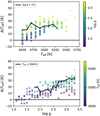 |
Fig. 5 Temperature offset obtained by assuming a log ɡ bias of +0.1 dex. Differences are plotted as a function of Teff (top panel) and log ɡ (bottom panel). The cases for Teff = 5000 K and log ɡ = 2.5 dex are highlighted by black lines. |
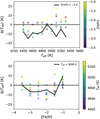 |
Fig. 6 Temperature offset obtained by assuming a [Fe/H] bias of +0.07 dex. Differences are plotted as a function of Teff (top panel) and [Fe/H] (bottom panel). The cases for Teff = 5000 K and [Fe/H]] = −2.0 dex are highlighted by black lines. |
4.2 Metallicity and microturbulence
To derive metallicity, the spectral fitting was done using the iSpec package (Blanco-Cuaresma et al. 2014), running the radiative transfer code Turbospectrum (Plez 2012) with spherical MARCS model atmospheres (Gustafsson et al. 2008) considering the atomic parameters of excitation potential and oscillator strength in Heiter et al. (2021). As proceeded in Paper I, we first derived the broadening parameters (microturbulence υmic and macroturbulence υmac). To this end, the projected rotational velocity υsin i was fixed to 1.6 km s−1 while υmic, υmac, and [Fe/H] were allowed to vary until the best global fit was obtained for all Fe lines. This gave us the first υmic estimate, which was then further tuned as described below. Several line lists from the literature were compiled to derive these parameters: Fe I and Fe II for giants from Jofré et al. (2014), the ‘ASPL’ and ‘MASH’ lists of Fe I from Dutra-Ferreira et al. (2016), and the Fe II line list from Meléndez & Barbuy (2009). As our method does not assume ionisation equilibrium, the abundance biases associated with some of these line lists and discussed in the papers mentioned above do not affect our results. More specifically, the capacity of our method to recover accurate Teff and log ɡ was evaluated by comparing its outcomes against those inferred by interferometric measurements in Paper I.
As demonstrated in Sect. 5, our set of Teff and log ɡ are statistically accurate, and therefore the accuracy of our set of iron abundances is mainly subject to potential systematic errors resulting from our Fe II line modelling6 carried out with 1D, spherically symmetric model atmospheres assuming LTE. Iron abundances were determined from Fe II lines, although abundances from Fe I lines were also derived to quantify the offsets induced by the LTE modelling; hereafter, we refer to [Fe II/H] when mentioning metallicity. Only weak lines were considered in our procedure to minimise 1D modelling of the defects. More precisely, we restricted lines with reduced equivalent width (REW = log(EW/λ)7) lower than −5 to make sure we work in the linear part of the curve of growth. For CEMP stars, we extended this upper limit to −4.80 because very few weak and unblended lines were available.
We verified the absence of correlation between [Fe/H] and REW for the determined υmic values using Fe I and Fe II lines altogether. In Sect. 5.5, we find that Fe I abundances are generally lower than Fe II abundances under LTE. This implies that υmic may vary depending on the group of lines used for its determination: either neutral, ionised, or neutral and ionised lines. On the other hand, this is further vindication of the use of only weak lines to derive Fe abundances, as they are only weakly sensitive to υmic, as already mentioned above. We exemplify this concept with the star HD 122563 in Fig. 7. The top panel shows no correlation between [Fe/H] and REW when both Fe I and Fe II are considered (solid red line). Only a small correlation appears when [Fe/H] is computed from Fe I lines (black dashed line). The bottom panel in the figure shows that this slope may be eliminated by increasing υmic to ~ 3.30 km s−1 or more. With υmic = 3.30 km s−1, the average [Fe I/H] abundance would decrease from −2.81 to −2.84 dex, whereas [Fe II/H] would remain equal to −2.71 dex. The total uncertainty of [Fe/H] is estimated in Sect. 5.5.
4.3 Surface gravity from Mg triplet lines
Conventional isochrones have a standard (solar) chemical composition scaled to the considered stellar metallicity. They are not adapted to determine log ɡ of stars with peculiar surface compositions, because the isochrone position is sensitive to the photospheric CNO abundances, as illustrated in Figs. 24 and 26 of Karinkuzhi et al. (2021). Indeed, a modified composition can affect the opacities, and therefore also the bolometric magnitude and the effective temperature.
Anticipating this problem, we derived surface gravities from the 5172 and 5183 Å magnesium triplet lines, which, unlike the 5167 Å line, are reasonably free from blends for most metal-poor stars. To determine the surface gravity from Mg lines, we synthesised spectra adopting the following parameters for each star: (i)  and (ii) [Fe II/H] as listed in Table 2, and (iii) log ɡ in the range [0.5–3.5] with a step of 0.5 dex. These grids were interpolated in log ɡ with a step of 0.01 dex. We considered two fitting windows located far from the line cores in order to avoid chromospheric effects. Wavelength regions with line blends were avoided.
For stars with [Fe/H] ≲ −2, Mg lines are relatively narrow (coverage less than 1 Å) and display asymmetries that 1D LTE models cannot reproduce. For these, we fixed the fitting windows to [5172.0–5172.5] Å and [5172.8–5173.4] Å for the line at 5172 Å, and to [5182.8–5183.45] Å and [5183.8–5184.1] Å for the line at 5183 Å. For CEMP stars, we set the limits of fitting windows to the regions without blends, always avoiding the line core (at a wavelength distance of at least +0.3 Å). An example of these windows for the CEMP star HD 76396 is illustrated on Fig. 8.
The fitting procedure is similar to that used for Hα. Each wavelength pixel inside the fitting windows is associated with the log ɡ of the most compatible interpolated synthetic profile. This generates a dispersion of log ɡ values, the histogram of which represents a probability distribution; see for example the right panels of Fig. 8. As in many cases it is only possible to fit a few wavelength bins, we do not directly fit Gaussians to the histograms, as done with Hα lines (see right panels in Figs. A.2–A.6). Instead, we estimate the most probable log ɡ and its error by bootstrap; that is, the log ɡ dispersion associated to the wavelength bins is randomly resampled (bootstrapped dataset), and its median and standard deviation are computed. This procedure is repeated 1000 times, and the mean of all computed medians is considered the most probable log ɡ, whereas the mean of all computed standard deviations is taken as its error. The total uncertainty on log ɡ is estimated in Sect. 5.4.
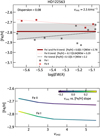 |
Fig. 7 Metallicity determination of the star HD 122563. Top panel: line-to-line Fe abundances computed with υmic = 2.5 km s−1 as a function of the reduced equivalent width. Grey and red dots represent Fe I and Fe II lines, respectively. The solid dark red line is the trend of all Fe I and Fe II measurements. The black dashed and red dotted lines are the trends of Fe I and Fe II measurements, respectively. The shade represents the dispersion. Bottom panel: for HD 122563, metallicity as function of υmic colour-coded by the slope of the trends in the υmic–[Fe/H] plane. |
4.4 Asteroseismic surface gravity
We cross-matched the ESO archive with the TESS catalogue (Stassun et al. 2018), searching for stars with asteroseismic measurements of maximum frequency (vmax) in Hon et al. (2021). We identified four stars with archived spectra of good S/N: HD 3179, HD 13359, HD 17072, and HD 221580. Their  , log ɡiso, log ɡMg, and [Fe/H] were derived as described in previous sections. We also included the stars TIC 168924748 and TIC 404605506 in this analysis, although we did not find archival spectra for them. These stars have an IRFM Teff (Casagrande et al. 2021) listed in the GALAH DR3 catalogue (Buder et al. 2021), which is determined here to be consistent with
  (Sect. 5.1). Therefore, along with the four stars above, they are suitable for determination of the accuracy of the log ɡiso and log ɡMg scales. These stars appear as dwarfs in our initial crossmatch according to their parameters in Stassun et al. (2018), where their log ɡ values are 4.49 and 4.48 dex, respectively. However, the GALAH catalogue indicates that they are giants, and their associated log ɡ values given in Table 1 were taken as preliminary. We verified in the STARHORSE catalogue (Anders et al. 2022) that these stars are most likely red giants; this catalogue provides log ɡ values 2.46 and 2.80 dex for TIC 168924748 and TIC 404605506, respectively.
We determine asteroseismic surface gravity (log ɡseis) using the expression:
 (2)
(2)
where we adopt the values vmax⊙ = 3090 µHz, Δv⊙ = 135.1 µHz, logg⊙ = 4.44 dex, and Teff⊙ = 5777 K (Huber et al. 2011). log ɡseis is compiled in Table 3 along with vmax derived by Hon et al. (2021). We used Δv⊙ along with the  errors in Table 2 and vmax errors in Table 3 to obtain log ɡseis errors. We include log ɡMg and log ɡiso in Table 3 for comparison.
4.5 Luminosity and radius
We computed luminosities (L) using the relation  , where L* is the luminosity of the star, L0 is the zero-point luminosity 3.0128 × 1028 W (Mamajek et al. 2015), and X and BCX are the absolute magnitude in a determined photometric band and its corresponding bolometric correction. Absolute magnitudes were computed from apparent magnitudes (extinction corrected as described in Paper I) and the distance estimates of Bailer-Jones et al. (2018), where the Gaia parallax zero-point correction (+0.021 mas, Lindegren et al. 2021) was considered. Bolometric corrections were computed for each of the Gaia magnitudes G, BP, and RP, which are extinction-corrected with the routine bcutil.py8 (Casagrande et al. 2014; Casagrande & VandenBerg 2018). Luminosities in Table 2 are average values obtained with every Gaia magnitude band; values relative to the Sun in logaritmic scale (log L/L⊙) are listed. The uncertainty on these values was computed by adding in quadrature the errors induced by the Teff, log ɡ, and [Fe/H] errors given in the table. Stellar radius (R) was computed from log (L/L⊙) and Teff in the table by means of the Stefan-Boltzmann relation; values relative to the Sun (R/R⊙) are listed. Its errors were expanded from log (L/L⊙) and Teff errors into the formula.
 |
Fig. 8 Magnesium profile fits of the CEMP star HD 76396. The observational profile is represented by the black line. The thick red line represents the fitted profile and shaded areas indicate the fitting windows. The right panels show histograms of the log ɡ values associated with all the pixels within the shaded windows. The most probable log ɡ and its error are obtained by bootstrapping; see main text. |
Giants with asteroseismic measurements.
5 Accuracy tests
5.1 Accuracy of Hα effective temperature
Assessing model-based Teff determinations can be done with the help of stars with angular diameters (θ) inferred via interferometry. Their Teff are considered to carry marginal model influence, and are therefore considered to lie on a scale that is close to accurate. The set of Gaia benchmarks compiled in Heiter et al. (2015) and Jofré et al. (2014) includes 34 nearby stars with interferometric Teff. Among them, only four have [Fe/H] < −1 dex, from which one is a red giant, HD 122563. This paucity was later mitigated by the incorporation of a subsample of ten stars with −2 ≲ [Fe/H] ≲ −1 dex provided by Hawkins et al. (2016), where two are red giants: HD 175305 and HD 218857. However, their temperatures were determined by means of the IRFM (Blackwell & Shallis 1977; Blackwell et al. 1979, 1980), which is relatively insensitive to model inaccuracies as well, as it makes use of photometry in the Rayleigh-Jeans spectral region.
We demonstrated in Paper I that Teff determinations from Hα fitting and from interferometrc measurements are compatible for a wide range of atmospheric parameters of F-, G-, and K-type stars. Furthermore, we demonstrated the excellent agreement between these Teff and the temperatures determined using the IRFM in the metallicity range −3 ≲ [Fe/H] ≲ −1 dex for dwarf and turnoff stars. However, the validation of Teff determinations using Hα was not tested for metal-poor giants given the paucity of benchmark stars of this category. Karovicova et al. (2020) recently provided interferometric Teff determinations for ten stars with [Fe/H] < −0.7 dex. Two of them are Gaia benchmarks, and the remaining are new standards, that is, six giants and two dwarfs.
Concerning IRFM, Casagrande et al. (2021) expanded the applicability range of the implementation in Casagrande et al. (2010) to the RGB. Some of these stars have been studied in the context of the ‘First Stars’ large programme9 and are available in the ESO archive.
Figure 9 shows the comparison between  and what we call ‘standard scale’, which represents either interferometric temperatures shown with red symbols, temperatures based on θ determined by calibrations with blue symbols (Cohen et al. 1999; Kervella et al. 2004), or IRFM temperatures with grey symbols. The stars tested in the present work are indicated by their labels in the top and bottom panels; the additional points are the benchmark stars of Paper I. For the sake of completeness of the comparisons, in the following discussion we include the subgiant metal-poor star HD 140283 with
  K derived in Paper I; its interferometric Teff is 5792 ± 55 K (Karovicova et al. 2020) and the IRFM Teff is 5777 ± 55 K (Casagrande et al. 2010).
The agreement between Hα and interferometric temperatures is excellent for HD 140283 and HD 122563, with negligible differences of ~20 K. For HD 2665, the difference is greater (124 K), but the interferometric and Hα temperatures are still in agreement within 1σ. For HD 175305 and HD 221170, the differences are 249 and 319 K, respectively, which are errors of between 1σ and 2σ. However, their reported interferometric errors are relatively large (2%–3%; see Table 1). HD 175305 also has an IRFM Teff (Hawkins et al. 2016), which is in much better agreement (40 K difference) with  (grey symbol linked to the red symbol by the dashed line in Fig. 9). Therefore, the interferometric temperature of HD 175305 seems to be underestimated. We now discuss whether this could also be the case for HD 221170, for which there is no accurate IRFM determination available in order to evaluate this possibility. Nevertheless, some evidence is provided in Casagrande et al. (2014), where systematic errors in interferometric temperatures are observed towards low θ values. In the analysis related to their Fig. 4, these authors explain that such systematic errors may arise for θ ≲ 0.9 mas due to the insufficient power of beam combiners for sampling the visibility curve of the star disc at its border, which requires high spatial frequencies. The bottom panel of our Fig. 9 shows similar systematic uncertainties to those in Fig. 4 of Casagrande et al. (2014). Examples of how the sampling at high frequency can dramatically improve angular diameter measurements were provided by White et al. (2013) in their comparison of the outcomes from the Michigan Infrared Combiner (MIRC, Monnier et al. 2004), the Classic combiner, and the Precision Astronomical Visible Observations (PAVO, Ireland et al. 2008) combiner at the Center for High Angular Resolution Astronomy (CHARA) array (ten Brummelaar et al. 2005). Casagrande et al. (2014) also comment on the outcomes for the solar twin 18 Sco (Porto de Mello & da Silva 1997) from PAVO by Bazot et al. (2011) and from Classic by Boyajian et al. (2012), where the latter presents significant systematic uncertainties. Although the angular diameter measurements of HD 2265, HD 175305, and HD 221170 were acquired with PAVO (Karovicova et al. 2020), which offers sampling at the highest frequency, it is possible that their visibility curves are still biased towards high counts at high frequencies. If so, their θ determination may be affected and this could be at the origin of the discrepancies between
  and interferometric temperatures of the three stars above.
We find that  and IRFM Teff agree for all stars in our red giant sample within 1 σ individual errors. This includes HD 140283 and HD 175305, with interferometric Teff compared above; for these we obtain
  -IRFM Teff values of +33 and +40 K, respectively. As shown in Fig. 9, no difference exceeds 76 K; this particular difference is seen for a star with a spectrum of moderately low quality in our sample, namely BPS CS 22892052 with S/N ~139. The median of the differences between
  and the IRFM Teff is +28 K (grey horizontal line in the upper panel of Fig. 9), which is close to the IRFM Teff zero-point uncertainty of 20 K estimated by Casagrande et al. (2010). For stars with interferometric data, we obtain a median difference of –11 K when the outliers HD 2265, HD 175305, and HD 22117 are omitted.
We conclude that Hα and IRFM temperatures are compatible for giants and dwarfs and show no significant systematic uncertainties with any atmospheric parameter nor with angular diameter, and therefore the outcomes of both methods are equivalent and can be averaged to improve imprecise  determinations due to low-S/N spectra, such as those of BPS CS 22892–052; see Table 2. Interferometric Teff should be used with caution for stars with angular diameters of lower than 1 mas, because in some cases it can be underestimated by a few hundred Kelvin. For such stars, effective temperatures are best derived using Hα fitting or IRFM.
We take the largest dispersion in Fig. 9, of namely ± 46 K, as the official uncertainty on the Hα 3D non-LTE model. However, we emphasise that the IRFM and interferometric Teff errors of the stars in the comparison are similar to or even larger than this quantity, and therefore they dominate the dispersion of the comparison. For this reason, the internal uncertainties in Table 2 are good estimates, and can be expanded in order to derive dependent parameters and abundances.
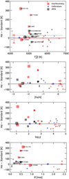 |
Fig. 9 Temperature difference as a function of the atmospheric parameters in Table 2 and the angular diameter in Table 1. The plots include the Gaia benchmarks (see Fig. 7 of Paper I). The stars for which |
 |
Fig. 10 Comparison between effective temperatures from the colour–Teff relations of Casagrande et al. (2021) and those derived by Hα in this work. Each column corresponds to one Gaia colour, and each row shows the distribution of the differences with respect to Teff, [Fe/H], and log ɡ, respectively. TITANS I dwarfs are plotted in blue, and CEMP stars are highlighted with dark contours. The symbol sizes are inversely proportional to log ɡ. Red lines connect medians computed in equally spaced bins, and vertical bars correspond to 1σ dispersions; their values are indicated in red characters. Medians and corresponding 1σ dispersions for only the giants (grey symbols) – omitting CEMP stars – are given in red characters. Giants with temperature differences of greater than 2σ are labelled with their catalogue numbers. |
5.2 Validation of IRFM-based Gaia photometric calibrations
Casagrande et al. (2021) provide colour–Teff calibrations based on the IRFM for about 590 000 stars in the GALAH DR3 catalogue with Gaia and 2MASS photometry. The zero-points were finely tuned with solar twins, and therefore the derived Teff are expected to be accurate for stars with parameters close to solar. The calibrations with the Gaia colours BP – RP, G – BP, and G – RP are of special interest for automatic Teff determinations for the large number of giants in the Gaia catalogue; they are expected to provide precise Teff for metal-poor stars with preliminary [Fe/H] and log ɡ (as those in Andrae et al. 2023), as they show little response to typical offsets in these parameters. Typically, ± 40–50 K is the combined effect of ∆log ɡ = 0.2, ∆[Fe/H] = 0.1, and ∆E(B – V) = 0.1. On the other hand, the performance of this calibration at the metal-poor range has not been rigorously quantified because of the lack of an extended sample of metal-poor reference stars; see Fig. 6 of Casagrande et al. (2021).
Here we test the performance of this calibration in the parameter range covered by our sample of metal-poor red giants. We derived colour-calibrated temperatures10 from Gaia colours by running the script colte11, using [Fe II/H] and log ɡ in Table 2, and E(B – V) in Table 1; the latter was extracted from either Stilism (Capitanio et al. 2017) when available or from Schlegel et al. (1998) otherwise. In order to obtain dereddened colours, the script colte converts E(B - V) to the Gaia system using extinction coefficients of either Schlafly & Finkbeiner (2011) or Cardelli et al. (1989) and O’Donnell (1994). We chose to use the former in the analysis below; we verified that when using the latter we obtain temperatures that differ by only a few Kelvin. Figure 10 compares the colour-calibrated temperatures with  as a function of the atmospheric parameters. For completeness, dwarf stars from Paper I are included in the analysis and represented in blue. We observe that the calibrations using BP – RP provide the best agreement with
  . As shown by the plots on the left column of Fig. 10, there is perfect agreement across the entire Teff–[Fe/H]-log ɡ parameter space. The calibrations with the G – BP colour agree with
  for giants, whereas they produce temperatures that are ~60 K hotter for dwarfs. The calibrations with the G – RP colour produce temperatures that are ~70 K cooler than
  for giants, whereas for dwarfs they can be ~ 100 K cooler. We note that, although small offsets for dwarfs between
  and the colour-calibrated temperature appear for G – BP and G – RP colours, we demonstrated in Paper I that IRFM temperatures (the basis of these colour calibrations) are fully compatible with
  .
.
Concerning CEMP stars, Fig. 10 illustrates the large discrepancies between their colour-calibrated temperatures and  , with differences larger than 2σ. More precisely, the C2 and CN absorption bands produce strong flux absorption, which is not taken into account in the photometric calibrations considering solar-scaled chemical abundances. Standard photometric calibrations can therefore produce strong biases when applied to CEMP stars.
5.3 Comparison of literature temperatures with accurate Teff
Disregarding the first three sections of Table 1, which contain standard stars for accuracy tests, several stars have temperatures derived with the colour–Teff relations of Alonso et al. (1996) in their respective source papers: Cayrel et al. (2004) and Carney et al. (2008). Preliminary temperatures of a few stars were derived by spectral fitting (Arentsen et al. 2019; Koleva & Vazdekis 2012; Beers et al. 2017), and several others were derived assuming excitation ionisation equilibrium of Fe lines (Johnson 2002; Hansen et al. 2018; Karinkuzhi et al. 2021).
Figure 11 shows the offsets between the literature temperatures and the Teff determined in Sect. 5.1. No general correlations with the atmospheric parameters are observed. Average differences, indicated by the horizontal lines, show that the three scales underestimate Teff by ~100 K. Casagrande et al. (2010, Fig. 3) found the same bias for the scale of Alonso et al. (1996) with dwarf stars; here we can verify that the same exists for red giants. Casagrande et al. (2010, Fig. 11) also found temperature underestimations similar to ours for the spectral fitting method when revising the catalogue of Valenti & Fischer (2005). Preliminary temperatures derived from the excitation and ionisation equilibrium of Fe lines show the greatest dispersion. Among them, the temperatures of four stars (HD 26, HD 5223, HD 201626, and HD 224959) differ with  by less than 120 K. However, these stars have literature log ɡ and [Fe/H] that differ from ours by up to 0.7 and 0.4 dex, respectively, in the worse cases (HD 5223 and HD 224959). It is therefore plausible that, due to the strong parameter interdependence that this method involves, biases permute among Teff, log ɡ, and [Fe/H] in a complicated manner that we cannot fully understand with our small and selection-biased sample. In Sects. 5.5 and 5.6, we demonstrate that the ionisation equilibrium of Fe is not satisfied under LTE for giants. We therefore indicate that this assumption is likely the main source of the biases displayed here.
5.4 Accuracy of surface gravity
Custom methods to constrain log ɡ, such as forcing the ionisation balance of Fe lines and isochrone fitting, may lead to unreliable outcomes for giant stars. In Sects. 5.5 and 5.6, we demonstrate that the problem with the former method is that Fe I and Fe II in red giants are generally unbalanced under LTE. When isochrone fitting is applied, it is generally assumed that log ɡ (or luminosity) varies with Teff, age, metallicity, and mass. Other parameters such as the mixing length, α element enhancement, atomic diffusion, and the helium abundance, for instance, are also relevant in the RGB (e.g. Song et al. 2018; Cassisi 2017; Cassisi & Salaris 2020), and may vary from one case to another in complicated and diverse manners that are generally not accounted for in ready-made isochrone grids such as those used in this work. As a consequence, the accuracy of log ɡ from isochrone fitting for field stars is uncertain and likely imprecise.
We evaluate the accuracy of log ɡiso and log ɡMg using log ɡseis in Table 3 as the reference scale. Figure 12 shows that log ɡMg and log ɡseis are compatible within 1σ errors for three stars out of four with measurements available, whereas log ɡiso significantly deviates to higher values for every star. Accordingly, we accept log ɡMg as the accurate surface gravity determination of our sample. Table 2 lists averaged values from both Mg triplet lines employed (5172 and 5183 Å) among our recommended parameters, and its errors are estimated below. We note that the stars in this test are constrained within a narrow log ɡ range between 2.40 and 2.50 dex. Therefore, the accuracy of our log ɡ in Table 2 is guaranteed within this range and in the near surroundings, that is, approximately + 0.5 dex. The accuracy of our recommended log ɡ values of lower than ~2 dex requires comparison with outcomes from fundamental methods on eclipsing binaries (e.g. Hełminiak et al. 2019; Ratajczak et al. 2021; Miller et al. 2022; Maxted 2023) or well-calibrated asteroseismology.
The determination of log ɡiso is straightforward and can still be useful when the log ɡMg determination is unfeasible, if indeed its offsets are well characterised. This is the case for the stars BPS CS 22186−025, BPS CS 22189−009, BPS CS 22891−209, BPS CS 22949−048, and BPS CS 22956−050, the Mg lines of which are too narrow to be used as log ɡ indicators. In Fig. 13, we compare the log ɡMg values obtained from each Mg line with log ɡiso; Table A.1 lists all values in the comparison. We reiterate here that the latter may only provide reasonable outcomes for non-enriched stars, and therefore CEMP stars are excluded from Fig. 13. The plots show no obvious correlation with any atmospheric parameter, but display systematic offsets. Even though the internal precision of the individual log ɡMg measurements worsens as metallicity decreases, as shown in the middle plot, the dispersions of the distributions remain roughly constant across the considered parameter range. As shown in the top panel of the figure, both Mg lines provide similar log ɡMg, and their offsets with respect to log ɡiso are almost identical. The average of these offsets is −0.34 dex, which we use as the correction factor for log ɡiso. To determine log ɡMg error, we assume that the dispersion of the difference between log ɡiso and the averaged log ɡMg values, of namely 0.17 dex, is composed from the addition in quadrature of the corresponding errors. As the typical log ɡiso error is 0.08 dex, the typical log ɡMg error is found to be 0.15 dex.
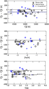 |
Fig. 11 Comparison between |
 |
Fig. 12 Surface gravity difference for each star in Table 3. log ɡiso and log ɡMg relative to log ɡseis are displayed in red and grey, respectively. |
5.5 Fe ionisation balance under LTE
The so-called ‘excitation and ionisation balance of Fe lines’ has been largely used as a standard method to determine atmospheric parameters; see a few recent examples in Hema et al. (2018); Hill et al. (2019), and Karinkuzhi et al. (2021). This method consists on assuming that the abundances derived from neutral and ionised Fe lines are identical. Such an assumption only leads to reliable log ɡ if the assumption of LTE is valid. Tsantaki et al. (2019) selected Fe II lines so that the iron ionisation balance is satisfied in their sample of F, G, and K solar-metallicity dwarfs; whether this configuration can be extrapolated to other spectral types and metallicities remains to be verified.
Ionised Fe lines have been observed to be virtually insensitive to departures from LTE (e.g. Fabrizio et al. 2012; Lind et al. 2012; Mashonkina et al. 2011; Sitnova et al. 2015) in F-, G-, and K-type stars. Moreover, Amarsi et al. (2016) showed that Fe II abundances remain almost the same whether derived from 1D LTE or 3D non-LTE models. These authors also observed that 3D non-LTE Fe I abundances are similar to those of Fe II. Therefore, Fe II lines can be safely used when fast 1D LTE calculations are performed.
Given the relatively large sample of metal-poor stars with accurate Teff and log ɡ compiled in Paper I and here, we examine the compatibility of Fe I and Fe II abundances under LTE throughout the Teff–log ɡ–[Fe/H] parameter space. The following analysis is relevant because, in many cases, only a few Fe II lines may be available in observational spectra due to severe blending. Figure 14 shows the comparison between the two abundance sets. The ionisation unbalance appears only for red giants; that is, stars with log ɡ ≲ 3.5 dex. The distributions of the abundance differences with Teff and log ɡ are relatively similar (see top and bottom plots of Fig. 14). Therefore, we infer that Fe I lines only allow reliable abundance determinations for main sequence stars up to the very beginning of the subgiant branch. For giants, Fe I lines certainly lead to abundance underestimations of between −0.10 and −0.20 dex (as shown by the red lines in the Teff and log ɡ ranges covered by the grey symbols in Fig. 14). We note that these offsets are only valid for Fe abundances derived from accurate Teff and log ɡ. The ionisation unbalance displays no correlation with respect to [Fe/H] in the analysed parameter space (see middle panel in Fig. 14). Assuming LTE ionisation balance for red giants could therefore lead to biased log ɡ determinations, and so this method should be avoided.
The above results confirm those of Karovicova et al. (2018). Sitnova et al. (2015) found that departures from ionisation equilibrium appear in dwarfs for [Fe/H] ≲ −1 dex (see Fig. 7 in the paper), which contradicts our results. In the analysis performed by these latter authors, Fe I abundances match Fe II when non-LTE models are used. We cannot determine what the source of their relatively low LTE Fe I values is. However, we note that their temperature scale is a possible source. Sitnova et al. (2015) derived temperatures with the colour calibrations of Ramírez & Meléndez (2005), which lead to temperatures that are ~ 100 K cooler than the IRFM scale of Casagrande et al. (2010; see Fig. 5 in the paper), which is compatible with ours; see Sect. 5.1 We determine the total precision of our [Fe/H] determination by accepting that the dispersion in Fig. 14 is the even contribu tion of the errors of [Fe I/Η] and [Fe II/H] added in quadrature As the dispersion is ~0.13 dex, we determine a [Fe/H] preci sion of ±0.09 dex. This is a little higher than the typical interns precision of ±0.05 dex, as it accounts for Teff and log ɡ errors.
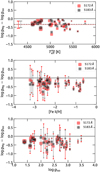 |
Fig. 13 Surface-gravity differences as a function of the atmospheric parameters. The size of each symbol is inversely proportional to log ɡiso. The points are coded in red or grey depending on the Mg I line (5172 Å or 5183 Å) used to compute log ɡMg log ɡiso In the top panel, the offsets and ± 1σ dispersions are represented by the dashed lines and error bars, the values of which are −0.35 ± 0.21 for the line at 5172 A (in red) and −0.33 ± 0.19 for the line at 5183 Å (in grey). Individual log ɡ values are listed in Table A.1. Error bars in the middle and bottom plots are the quadratic sum of the errors of log ɡiso and those of log ɡMg |
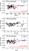 |
Fig. 14 Deviation from ionisation balance as a function of the atmospheric parameters. Dwarf stars from Paper I are plotted in blue, and CEMP stars are highlighted with dark contours. The symbol sizes are inversely proportional to log ɡ. The red lines in the top and bottom panels connect medians computed in equally spaced bins of Teff and log ɡ, respectively; medians and bin sizes are indicated in the plots. The vertical bars correspond to 1σ standard deviations; the corresponding values are indicated in the plots as well. |
5.6 Fe ionisation balance under non-LTE
Spectral synthesis with iron in non-LTE was performed using Turbospectrum 202012 (Gerber et al. 2023) for three MARCS model atmospheres with parameters close to those of the star HD 122563, BD+ 11 2998, and BPS CS 29502−042, which have atmospheric parameters that are representative of the sample. We first extracted the iron departure coefficients – based on the iron model atom developed in Bergemann et al. (2012) and Semenov et al. (2020) – corresponding to the three atmospheric mod els. Then, using the curated line list from the Gaia-ESO Survey (Heiter et al. 2021), we computed synthetic spectra in the range 4900–6500 Å with a step of 0.005 Å, both in LTE and non-LTE, varying the iron abundance by steps of 0.1 dex.
With these spectra, we compare non-LTE with LTE abundances, performing a differential line-by-line analysis. To this end, we used the same input parameters, the same line lis for non-LTE and for LTE models, and we ran the same fitting algorithm. Our analysis only considers lines with log(EW/λ) ≤ −5. As expected, for Fe II, we obtain the same outcomes with LTE and non-LTE models. Individual abundances of Fe I line obtained in LTE and non-LTE are compared in Fig. 15. We note that taking into account non-LTE effects shifts the Fe ι line abundances up by ~0.12 dex and brings them into agreement with the Fe II line abundances within 1σ. Accordingly, non-LTE Fe I and LTE Fe II can be averaged, or one can be used in absence of the other for stars in the parameter range analysed here.
6 Mg, C, N, and О abundances
Element abundances were derived assuming the following atmospheric parameters:  , [Fe II/Η], and log ɡ in Table 2.
6.1 Magnesium
Magnesium was derived primarily from the line at 5711 Å. This line has been shown to be little affected by 3D non-LTE effects, both theoretically (Mashonkina 2013; Bergemann et al. 2017a and observationally (Giribaldi & Smiljanic 2023b). In case where this line was not available, either because it was too weal or because it was not covered by the spectrum, we used the line at 5528 Å instead. Figure 16 shows abundance discrepancies between these lines as a function of [Fe/H], A(Mg)13, and the difference between the reduced equivalent widths14 of the Mg lines ∆(REW) = log(EW/5528) – log(EW/5711). In the bottom panel the symbols are colour-coded according to a logarithm scale оf the reduced equivalent width of the line at 5528 Å. In general we find that discrepancies remain moderate, at around 0.1 dex. This is true for most stars with [Fe/H] ≲ –1 dex, as shown by the top panel in the figure. At low ∆(REW), the abundance from the line at 5528 Å tend to be lower than those from the line at 5711 Å (darkest grey symbols). This is the case for stars with the highest metallicities and Mg abundances: HD 105740 and BD+11 2998, as the top and middle panels show. Similar outcomes are also observed in dwarfs (Giribaldi & Smiljanic 2023b). We note that in the present case, abundance discrepancies remain small even for high ∆(REW) values (≲ 0.6) because their Mg lines are unsaturated. As the red symbols in the bottom panel of the figure show, the REW of the strongest line, 5528 Å, remains lower than −4.8, and therefore remains within the linear section of the so called curve of growth.
We use the exponential fits in the middle panel to correct the offsets carried by the Mg determinations from the 5528 Å line; thus, Mg of all TITANS, dwarfs, and giants lies in the same scale. Finally, we adopt the non-LTE correction to all Mg abundances of Mashonkina (2013) for the line 5711 Å. This is +0.07 dex, which is an average of the ‘Darwinian rates scaled values’ (defined so by the authors) for [Fe/H] = −1 and [Fe/H] =−2 dex given in Table 5 of this latter paper. Corrections were also provided by Merle et al. (2011), but not for all the atom parameters. We note that the abundance discrepancies shown in Fig. 16 are only valid when line synthesis is applied. Abundance determination via EW measurement likely produces different outcomes.
The uncertainties of the abundances are computed as described in Giribaldi & Smiljanic (2023b). Namely, we produced grids of A(Mg) offsets induced by typical offsets of Teff, log ɡ, [Fe/H], and log ɡ. To this end, we first synthesised spectra around the lines 5528 and 5711 Å. The spectra were produced with four values of Teff between 4500 and 6000 K, three values of log ɡ between 1 and 3 dex, four values of [Fe/H] between −3 and −0.5 dex, seven values of A(Mg) between 4.8 and 7.2 dex, and two values of vmic between 1 and 2 km s−1. Subsequently, we computed abundances varying Teff, log ɡ, [Fe/H], and vmic, one at a time by their typical errors. These are ±50 K in Teff, ±0.15 dex in log ɡ, ±0.13 dex in [Fe/H], and ±0.3 km s−1 in vmic. Therefore, four grids of offsets with 672 spectra for each Mg line are available. We interpolated these grids with the atmospheric parameters of each star in Table 2 to compute their A(Mg) errors. As the grids provide offsets induced by ±50 K, the A(Mg) errors corresponding to the Teff errors in Table 2 are obtained by computing the required quantity. For example, for a Teff error of ± 100 K, the error provided by the grid must be multiplied by two. The typical A(Mg) error induced by  errors in Table 2 is ±0.05 dex, whereas those induced by log ɡ, [Fe/H], and υmic are of the order of 10−3, and were therefore neglected; Fig. A.7 shows the distribution of the offsets as a function of the atmospheric parameters. This error, ±0.05 dex, is therefore considered to be the typical A(Mg) error associated to the errors of all atmospheric parameters combined. This quantity is slightly smaller than the standard deviation of the abundance difference in Fig. 16, which is ±0.07 dex. Assuming this quantity is the result of the addition in quadrature of A(Mg) errors induced by the atmospheric parameters and the normalisation uncertainty due to spectral noise, we derive this latter to be ±0.05 dex. Therefore, we add the latter in quadrature to the A(Mg) error induced by
  to compute the total A(Mg) error given in Table 2.
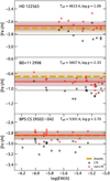 |
Fig. 15 Inferred iron abundance versus the ratio between equivalent width and wavelength for selected Fe I lines. Horizontal lines represent the averages of the symbols with the same colours. Dashed lines represent [Fe II/H] abundances. Shades represent 1σ dispersions around average values for non-LTE Fe I (red colour tone), and Fe II (yellow colour tone). |
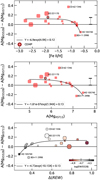 |
Fig. 16 Consistency of Mg abundance from the lines 5528 and 5711 Å. The top panel shows abundance differences as a function of metallicity, the middle panel displays the same differences as a function of the Mg abundance of the 5711 A line, and the bottom panel shows these differences as a function of the difference between log(EW5528Å/5528) and log(EW5711Å/5711). Symbols are colour-coded according to the reduced equivalent width of the line 5528 A in logarithmic scale. Symbols sizes are inversely proportional to log ɡ. Exponentials are fitted to the distributions in all panels. Stars with the largest discrepancies are tagged by their identifiers. 1σ errors (±0.07) around the average (+0.07) are represented by the error bars. |
 |
Fig. 17 Spectral fits for the determination of С in the C2 band (top panel), of the 12C to 13C ratio (middle panel), and of N in the CN band (bottom panel). Black lines represent the observational spectrum of HD 76396, blue lines represent the best modelled spectrum with abundances given in the legends, and green and red dotted lines represent modelled spectra with other abundances. |
6.2 Carbon, nitrogen, and oxygen
C, N, and О abundances were derived following the strategy in Karinkuzhi et al. (2021). We performed LTE spectral synthesis using Turbospectrum with spherical MARCS model atmospheres (Gustafsson et al. 2008) considering the line-list of Heiter et al. (2021). Oxygen was determined by fitting the triplet at 7771–7775 Å. We did not determine С and N abundances by individual line fitting as for Fe, Mg, and О, but instead fitted molecular band regions. To this end, we adapted a minimum χ2 routine, where grids of synthetic spectra were interpolated, varying the abundance of a given element. We derived C2 from the 5626–5634.5 Å region (avoiding the band-head at 5635 Å), as it appears less saturated than the 5155–5164 Å region, although similar abundances were obtained. The 12C/13C ratio was derived by fitting the 4737.5−4744 Å region and the 13C line at 8016.429 Å, which appears reasonably free from blends. Nitrogen abundance was derived by fitting either the 6305–6330 Å or 6345–6378 Å region once С was determined. Figure 17 shows an example of the spectral fitting for the determination of C, N, O, and the 12C/13C ratio for HD 76396. Table 4 lists CNO abundances derived for CEMP stars and their errors induced by the Teff, log ɡ, and [Fe/H] errors in Table 2, separately.
As shown in Fig. 18, all our CEMP stars are indeed enriched in carbon, most of them with [C/Fe] > 1, and are consistent with the higher-metallicity, upper carbon plateau (at A(C) ~ 8.25) as identified by Spite et al. (2013). This is expected, given that this region seems to contain mainly CEMP-s (and -sr) objects (Hansen et al. 2015a; Bonifacio et al. 2018). On the contrary, for lower metallicities ([Fe/H] < −3.4), the carbon abundance drops below A(C) = 7.6 (Bonifacio et al. 2018) and this region seems to contain mainly CEMP-no objects.
 |
Fig. 18 CEMP star carbon abundances, A(C), as a function of [Fe/H], The solar A(C) corresponds to the Sun photospheric determination in Grevesse et al. (2007). |
7 Conclusions
We provide accurate and precise atmospheric parameters (Teff log ɡ, and [Fe/H]) and Mg, C, N, and О abundances for 47 metal-poor red giant stars (Table 2). We refer to this sample of benchmark metal-poor stars, along with the metal-poor dwarfs of Giribaldi et al. (2021), as the TITANS reference stars. For 34 stars of this sample, the derived parameters are particularly precise, with total uncertainties of 40–80 K in Teff, 0.15 dex in log ɡ, 0.09 dex in [Fe/H], and 0.07 dex in A(Mg). We tested the accuracy of the derived atmospheric parameters with most of the (few) standard metal-poor stars available for which there are either new HERMES spectra or spectra recoverable from the ESO archives. We summarise the arguments in support of the Teff, log ɡ, and [Fe/H] determination accuracy below.
We derived effective temperatures ( ) by fitting observational Hα line profiles with 3D non-LTE synthetic models (Amarsi et al. 2018). The evaluation of the accuracy of
  is graphically summarised in Fig. 9, where the reference temperatures are either from interferometry (red symbols) or IRFM (dark symbols). The three scales are consistent and can be considered equivalently accurate. This is consistent with results obtained by Giribaldi et al. (2021) for dwarfs. We adopt the dispersion of the comparison in the figure, ±46 K, as the uncertainty of the 3D non-LTE Hα model for giants. The outlier stars HD 2665, HD 221170, and HD 175305 have relatively low interferometric Teff values, which are likely effects of small angular diameter offsets; see Sect. 5.1 for details.
Based on the outcome above, we evaluate the accuracy of the colour-dependent Teff relations of Casagrande et al. (2021) currently available for Gaia photometry. The evaluation is summarised in Fig. 10, where we observe excellent agreement for BP – RP and G – BP colours, disregarding CEMP stars. Table 2 lists a second set of temperatures derived by other methods found to correspond with  . These can be averaged with Teff to obtain more precise Teff for the TITANS. When available, we selected temperatures derived by the most direct of the three methods, which we rank in the following order: (1) inter-ferometry15, (2) IRFM, and (3) photometric calibrations using BP – RP.
We provide surface gravities derived by fitting Mg I b triplet lines at 5172 and 5183 Å. We verified their accuracy with stars with asteroseismic gravities; see Fig 12. Surface gravities from Yonsey-Yale isochrones (Kim et al. 2002; Yi et al. 2003) were found to be consistently higher by ~0.35 dex along the parameter space analysed; see Fig. 13. Nevertheless, in the absence of Mg triplet lines, they can be used to derive accurate log ɡ by subtracting the given offset.
We provide iron abundances from neutral and ionised species. We show in Sect. 5.5 that, provided accurate Teff and log ɡ fix inputs, LTE model atmospheres predict ionisation unbalance with [Fe I/H] abundances constantly lower than [Fe II/H] by ~0.15 dex, within the parameter space analysed for giants; see Fig. 14. We confirm in Sect. 5.6 that non-LTE models restore the ionisation balance to within typical uncertainties (~0.05 dex), whereas [Fe II/H] under LTE and non-LTE are almost equal; see Fig. 15.
We provide Mg abundances for all stars in the sample, and CNO abundances for the CEMP stars. The Mg abundances of all the stars in our sample are based on the scale of the 5711 Å line, and were corrected for non-LTE effects. We show that Mg abundances from the lines 5528 and 5711 Å under LTE may differ substantially depending on the stellar metallicity and the Mg abundance itself; see Fig. 16. The highest discrepancies are found for the highest metallicity ([Fe/H] ≳ −1 dex) and abundances (A(Mg) ≳ 7 dex), which is similar to the case of dwarfs (Giribaldi & Smiljanic 2023b, Fig. 3). The [C/Fe] rates in all CEMP stars are higher than 1, except for in HD 26, the most metal-rich star in the sample and a spectroscopic binary as well. The heavy elements of CEMP stars will be presented in Giribaldi et al. (in prep.).
A few TITANS seem to have started on a path towards the horizontal branch (HB), namely BD+17 3248, BD+09 2860, CD–41 15048, CD–62 1346, BD+11 2998, and HD 196944, the latter being a CEMP star; they are tagged in the HR diagram of Fig. 2. BD+17 3248 appears to be a genuine HB star, and has already been labelled as such, although with significantly higher Teff and lower log ɡ values (For & Sneden 2010). The other five stars show signs of binarity: CD–41 15048, BD+09 286, and BD+11 2998 show proper motion accelerations from HIPPARCOS and Gaia’s astrometric data (Kervella et al. 2019; Brandt 2021); CD–62 1346 shows significant variation of its radial velocity (Escorza et al. 2019); and HD 196944 is certainly a spectroscopic binary (Karinkuzhi et al. 2021). Our observational Teff and luminosities show that CEMP stars are rather located towards the right of the normal red giant branch stars, which is supported by the STAREVOL evolutionary tracks specifically computed for CEMP stars (Siess & Arnould 2008).
We recommend the use of [Fe I/H] in Table 2 only for reproducing observational Fe I lines via synthesis under LTE, whereas [Fe II/H] are accurate quantities required for evolutionary analysis of stellar populations. Similarly, we recommend the use of A(Mg) in Table 2 corrected by −0.07 to reproduce observational lines under LTE, as the quantities listed are corrected for non-LTE effects.
Finally, we recommend avoiding the use of the excitation and ionisation equilibrium of Fe and spectral fitting under LTE to simultaneously derive Teff, log ɡ, and [Fe/H] in metalpoor giants. These will likely provide biased determinations, as demonstrated in this work. Temperature outcomes of these two spectroscopic methods are consistent with those from the colour–Teff relations of Alonso et al. (1996). However, all are biased to cooler values; see also Casagrande et al. (2010), who obtained the same offset as that seen here. Users may confidently upgrade their methods for fast Teff determination using the Gaia colour–Teff relations with BP – RP and G – BP (Casagrande et al. 2021) for giants, and preferably with BP – RP for dwarfs. Alternatively, the differential spectroscopic approach (e.g. Meléndez et al. 2012; Reggiani et al. 2016) can be used with one or more TITANS as standards.
Element abundances of the CEMP stars
Acknowledgements
R.E.G. acknowledges the support by Fonds de la Recherche Scientifique (F.R.S.-FNRS) and the Fonds Wetenschappelijk Onderzoek-Vlaanderen (FWO) under the EOS programme (numbers 0.0004.22 and O022818F). R.E.G. acknowledges Ana Consuelo Giribaldi Santamaria for her incessant encouragement. S.V.E. thanks the Fondation ULB for its support. T.M. is granted by the BELSPO Belgian federal research program FED-tWIN under the research profile Prf-2020-033_BISTRO. This work is based on observations collected at the European Southern Observatory under ESO programmes: 074.B-0639(A), 68.D-0546(A), 165.N-0276(A), 0103.A-9013(A), 0104.A-9005(A), 097.A-9024(A), 68.B-0618(A), 65.N-0534(A), 167.D-0173(A), 076.B-0055(A), 072.C-0488(E), 090.B-0605(A), 076.B-0055(A), 072.B-0585(A), 083.B-0281(A), 0103.D-0310(A), 68.D-0546(A), 0104.D-0059(A), 079.D-0567(A), 078.B-0238(A), 080.D-0333(A). Use was made of the Simbad database, operated at the CDS, Strasbourg, France, and of NASA’s Astrophysics Data System Bibliographic Services. This research used Astropy (http://www.astropy.org) a community-developed core Python package for Astronomy (Astropy Collaboration 2018). This work presents results from the European Space Agency (ESA) space mission Gaia. Gaia data are processed by the Gaia Data Processing and Analysis Consortium (DPAC). Funding for the DPAC is provided by national institutions, in particular the institutions participating in the Gaia MultiLateral Agreement (MLA). The Gaia mission website is https://www.cosmos.esa.int/gaia. The Gaia archive website is https://archives.esac.esa.int/gaia. The Mercator telescope is operated thanks to grant number G.0C31.13 of the FWO under the “Big Science” initiative of the Flemish government. Based on observations obtained with the HERMES spectrograph, supported by the Fund for Scientific Research of Flanders (FWO), the Research Council of K.U. Leuven, the Fonds National de la Recherche Scientifique (F.R.S.- FNRS), Belgium, the Royal Observatory of Belgium, the Observatoire de Genève, Switzerland and the Thüringer Landessternwarte Tautenburg, Germany.
Appendix A Additional tables and figures
 |
Fig. A.1 Examples of the initial selection of red giants with UVES spectra in the ESO archive. The left panel displays stars with spectra of 200 ≤ S/N≤ 300, whereas the right panel shows stars with S/N > 300. The limits set are to separate main sequence stars (grey symbols) from red giant candidates (red symbols) and are arbitrary. |
 |
Fig. A.2 Hα profile fits of stars with interſerometric measurements. Left panels: Observational spectra are in black, whereas fitted synthetic Ha lines are represented by red continuous lines. A synthetic profile with −200 K is represented by the red dashed line to provide a view of the sensitivity of the flux along the wavelength axis. Shades indicate the windows of fits without metal or telluric lines. Right panels: Histograms of the temperatures associated to each wavelength bin inside of the windows of the fits. Gaussians fitted to the histograms are represented in black, whose peak centers and 1σ dispersions are indicated in red. They correspond to the determined |
Magnesium abundances and surface gravities.
 |
Fig. A.7 A(Mg) offsets induced by a −50 K Teff offset when derived from the line at 5711 Å. The horizontal line represents no offset. ‘X’ represents the element Mg in this case. |
References
- Alonso, A., Arribas, S., & Martinez-Roger, C. 1996, A&AS, 117, 227 [NASA ADS] [CrossRef] [EDP Sciences] [Google Scholar]
- Amarsi, A. M., Lind, K., Asplund, M., Barklem, P. S., & Collet, R. 2016, MNRAS, 463, 1518 [NASA ADS] [CrossRef] [Google Scholar]
- Amarsi, A. M., Nordlander, T., Barklem, P. S., et al. 2018, A&A, 615, A139 [NASA ADS] [CrossRef] [EDP Sciences] [Google Scholar]
- Amarsi, A. M., Nissen, P. E., & Skúladóttir, Á. 2019, A&A, 630, A104 [NASA ADS] [CrossRef] [EDP Sciences] [Google Scholar]
- Amarsi, A. M., Liljegren, S., & Nissen, P. E. 2022, A&A, 668, A68 [NASA ADS] [CrossRef] [EDP Sciences] [Google Scholar]
- Anders, F., Khalatyan, A., Queiroz, A. B. A., et al. 2022, A&A, 658, A91 [NASA ADS] [CrossRef] [EDP Sciences] [Google Scholar]
- Andrae, R., Fouesneau, M., Sordo, R., et al. 2023, A&A, 674, A27 [CrossRef] [EDP Sciences] [Google Scholar]
- Arentsen, A., Prugniel, P., Gonneau, A., et al. 2019, A&A, 627, A138 [NASA ADS] [CrossRef] [EDP Sciences] [Google Scholar]
- Astropy Collaboration (Price-Whelan, A. M., et al.) 2018, AJ, 156, 123 [Google Scholar]
- Bailer-Jones, C. A. L., Rybizki, J., Fouesneau, M., Mantelet, G., & Andrae, R. 2018, AJ, 156, 58 [Google Scholar]
- Bazot, M., Ireland, M. J., Huber, D., et al. 2011, A&A, 526, A4 [Google Scholar]
- Beers, T. C., & Christlieb, N. 2005, ARA&A, 43, 531 [NASA ADS] [CrossRef] [Google Scholar]
- Beers, T. C., Placco, V. M., Carollo, D., et al. 2017, ApJ, 835, 81 [NASA ADS] [CrossRef] [Google Scholar]
- Bell, R. A., Paltoglou, G., & Tripicco, M. J. 1994, MNRAS, 268, 771 [NASA ADS] [CrossRef] [Google Scholar]
- Bergemann, M., Lind, K., Collet, R., Magic, Z., & Asplund, M. 2012, MNRAS, 427, 27 [Google Scholar]
- Bergemann, M., Collet, R., Amarsi, A. M., et al. 2017a, ApJ, 847, 15 [NASA ADS] [CrossRef] [Google Scholar]
- Bergemann, M., Collet, R., Schönrich, R., et al. 2017b, ApJ, 847, 16 [Google Scholar]
- Blackwell, D. E., & Shallis, M. J. 1977, MNRAS, 180, 177 [NASA ADS] [CrossRef] [Google Scholar]
- Blackwell, D. E., Shallis, M. J., & Selby, M. J. 1979, MNRAS, 188, 847 [NASA ADS] [CrossRef] [Google Scholar]
- Blackwell, D. E., Petford, A. D., & Shallis, M. J. 1980, A&A, 82, 249 [NASA ADS] [Google Scholar]
- Blanco-Cuaresma, S., Soubiran, C., Heiter, U., & Jofré, P. 2014, A&A, 569, A111 [CrossRef] [EDP Sciences] [Google Scholar]
- Bohlin, R. C. 2007, in ASP Conf. Ser., 364, The Future of Photometric, Spectrophotometric and Polarimetric Standardization, ed. C. Sterken, 315 [Google Scholar]
- Bonifacio, P., Caffau, E., Spite, M., et al. 2018, A&A, 612, A65 [NASA ADS] [CrossRef] [EDP Sciences] [Google Scholar]
- Boyajian, T. S., McAlister, H. A., van Belle, G., et al. 2012, ApJ, 746, 101 [Google Scholar]
- Brandt, T. D. 2021, ApJS, 254, 42 [NASA ADS] [CrossRef] [Google Scholar]
- Buder, S., Asplund, M., Duong, L., et al. 2018, MNRAS, 478, 4513 [Google Scholar]
- Buder, S., Sharma, S., Kos, J., et al. 2021, MNRAS, 506, 150 [NASA ADS] [CrossRef] [Google Scholar]
- Capitanio, L., Lallement, R., Vergely, J. L., Elyajouri, M., & Monreal-Ibero, A. 2017, A&A, 606, A65 [NASA ADS] [CrossRef] [EDP Sciences] [Google Scholar]
- Cardelli, J. A., Clayton, G. C., & Mathis, J. S. 1989, ApJ, 345, 245 [Google Scholar]
- Carney, B. W., Latham, D. W., Stefanik, R. P., & Laird, J. B. 2008, AJ, 135, 196 [NASA ADS] [CrossRef] [Google Scholar]
- Carrera, R., Pancino, E., Gallart, C., & del Pino, A. 2013, MNRAS, 434, 1681 [NASA ADS] [CrossRef] [Google Scholar]
- Casagrande, L., & VandenBerg, D. A. 2018, MNRAS, 479, L102 [NASA ADS] [CrossRef] [Google Scholar]
- Casagrande, L., Portinari, L., & Flynn, C. 2006, MNRAS, 373, 13 [Google Scholar]
- Casagrande, L., Ramírez, I., Meléndez, J., Bessell, M., & Asplund, M. 2010, A&A, 512, A54 [NASA ADS] [CrossRef] [EDP Sciences] [Google Scholar]
- Casagrande, L., Portinari, L., Glass, I. S., et al. 2014, MNRAS, 439, 2060 [Google Scholar]
- Casagrande, L., Lin, J., Rains, A. D., et al. 2021, MNRAS, 507, 2684 [NASA ADS] [CrossRef] [Google Scholar]
- Casali, G., Magrini, L., Frasca, A., et al. 2020, A&A, 643, A12 [NASA ADS] [CrossRef] [EDP Sciences] [Google Scholar]
- Cassisi, S. 2017, in Eur. Phys. J. Web Conf., 160, 04002 [Google Scholar]
- Cassisi, S., & Salaris, M. 2020, A&ARv, 28, 5 [Google Scholar]
- Cayrel, R., Depagne, E., Spite, M., et al. 2004, A&A, 416, 1117 [NASA ADS] [CrossRef] [EDP Sciences] [Google Scholar]
- Cayrel de Strobel, G. 1996, A&ARv, 7, 243 [CrossRef] [Google Scholar]
- Cayrel de Strobel, G., & Bentolila, C. 1989, A&A, 211, 324 [NASA ADS] [Google Scholar]
- Cohen, M., Walker, R. G., Carter, B., et al. 1999, AJ, 117, 1864 [Google Scholar]
- Cui, X.-Q., Zhao, Y.-H., Chu, Y.-Q., et al. 2012, Res. Astron. Astrophys., 12, 1197 [Google Scholar]
- Dalton, G. 2016, in ASP Conf. Ser., 507, Multi-Object Spectroscopy in the Next Decade: Big Questions, Large Surveys, and Wide Fields, ed. I. Skillen, M. Balcells, & S. Trager, 97 [Google Scholar]
- Dalton, G., Trager, S., Abrams, D. C., et al. 2016, SPIE Conf. Ser., 9908, 99081G [Google Scholar]
- de Jong, R. S., Agertz, O., Berbel, A. A., et al. 2019, The Messenger, 175, 3 [NASA ADS] [Google Scholar]
- Dekker, H., D’Odorico, S., Kaufer, A., Delabre, B., & Kotzlowski, H. 2000, SPIE Conf. Ser., 4008, 534 [Google Scholar]
- De Silva, G. M., Freeman, K. C., Bland-Hawthorn, J., et al. 2015, MNRAS, 449, 2604 [NASA ADS] [CrossRef] [Google Scholar]
- Dutra-Ferreira, L., Pasquini, L., Smiljanic, R., Porto de Mello, G. F., & Steffen, M. 2016, A&A, 585, A75 [NASA ADS] [CrossRef] [EDP Sciences] [Google Scholar]
- Escorza, A., Karinkuzhi, D., Jorissen, A., et al. 2019, A&A, 626, A128 [NASA ADS] [CrossRef] [EDP Sciences] [Google Scholar]
- Fabrizio, M., Merle, T., Thévenin, F., et al. 2012, PASP, 124, 519 [NASA ADS] [CrossRef] [Google Scholar]
- For, B.-Q., & Sneden, C. 2010, AJ, 140, 1694 [NASA ADS] [CrossRef] [Google Scholar]
- Gaia Collaboration (Prusti, T., et al.) 2016, A&A, 595, A1 [NASA ADS] [CrossRef] [EDP Sciences] [Google Scholar]
- Gaia Collaboration (Vallenari, A., et al.) 2023, A&A, 674, A1 [NASA ADS] [CrossRef] [EDP Sciences] [Google Scholar]
- Gallagher, A. J., Bergemann, M., Collet, R., et al. 2020, A&A, 634, A55 [NASA ADS] [CrossRef] [EDP Sciences] [Google Scholar]
- Gerber, J. M., Magg, E., Plez, B., et al. 2023, A&A, 669, A43 [NASA ADS] [CrossRef] [EDP Sciences] [Google Scholar]
- Gilmore, G., Randich, S., Asplund, M., et al. 2012, The Messenger, 147, 25 [NASA ADS] [Google Scholar]
- Gilmore, G., Randich, S., Worley, C. C., et al. 2022, A&A, 666, A120 [NASA ADS] [CrossRef] [EDP Sciences] [Google Scholar]
- Giribaldi, R. E., & Smiljanic, R. 2023a, Exp. Astron., 55, 117 [NASA ADS] [CrossRef] [Google Scholar]
- Giribaldi, R. E., & Smiljanic, R. 2023b, A&A, 673, A18 [NASA ADS] [CrossRef] [EDP Sciences] [Google Scholar]
- Giribaldi, R. E., Porto de Mello, G. F., Lorenzo-Oliveira, D., Amôres, E. B., & Ubaldo-Melo, M. L. 2019a, A&A, 629, A33 [NASA ADS] [CrossRef] [EDP Sciences] [Google Scholar]
- Giribaldi, R. E., Ubaldo-Melo, M. L., Porto de Mello, G. F., et al. 2019b, A&A, 624, A10 [NASA ADS] [CrossRef] [EDP Sciences] [Google Scholar]
- Giribaldi, R. E., da Silva, A. R., Smiljanic, R., & Cornejo Espinoza, D. 2021, A&A, 650, A194 [NASA ADS] [CrossRef] [EDP Sciences] [Google Scholar]
- Gray, R. O. 2007, in ASP Conf. Ser., 364, The Future of Photometric, Spec-trophotometric and Polarimetric Standardization, ed. C. Sterken, 305 [Google Scholar]
- Grevesse, N., Asplund, M., & Sauval, A. J. 2007, Space Sci. Rev., 130, 105 [Google Scholar]
- Gruyters, P., Nordlander, T., & Korn, A. J. 2014, A&A, 567, A72 [NASA ADS] [CrossRef] [EDP Sciences] [Google Scholar]
- Gustafsson, B., Edvardsson, B., Eriksson, K., et al. 2008, A&A, 486, 951 [NASA ADS] [CrossRef] [EDP Sciences] [Google Scholar]
- Hansen, T., Hansen, C. J., Christlieb, N., et al. 2015a, ApJ, 807, 173 [Google Scholar]
- Hansen, T. T., Andersen, J., Nordstrom, B., et al. 2015b, A&A, 583, A49 [NASA ADS] [CrossRef] [EDP Sciences] [Google Scholar]
- Hansen, T. T., Holmbeck, E. M., Beers, T. C., et al. 2018, ApJ, 858, 92 [Google Scholar]
- Hawkins, K., Jofré, P., Heiter, U., et al. 2016, A&A, 592, A70 [NASA ADS] [CrossRef] [EDP Sciences] [Google Scholar]
- Heiter, U., Jofré, P., Gustafsson, B., et al. 2015, A&A, 582, A49 [NASA ADS] [CrossRef] [EDP Sciences] [Google Scholar]
- Heiter, U., Lind, K., Bergemann, M., et al. 2021, A&A, 645, A106 [EDP Sciences] [Google Scholar]
- Hełminiak, K. G., Konacki, M., Maehara, H., et al. 2019, MNRAS, 484, 451 [Google Scholar]
- Hema, B. P., Pandey, G., & Srianand, R. 2018, ApJ, 864, 121 [NASA ADS] [CrossRef] [Google Scholar]
- Hill, V., Skúladóttir, Á., Tolstoy, E., et al. 2019, A&A, 626, A15 [NASA ADS] [CrossRef] [EDP Sciences] [Google Scholar]
- Hon, M., Huber, D., Kuszlewicz, J. S., et al. 2021, ApJ, 919, 131 [NASA ADS] [CrossRef] [Google Scholar]
- Huber, D., Bedding, T. R., Stello, D., et al. 2011, ApJ, 743, 143 [Google Scholar]
- Ireland, M. J., Mérand, A., ten Brummelaar, T. A., et al. 2008, SPIE Conf. Ser., 7013, 701324 [NASA ADS] [Google Scholar]
- Jofré, P., Heiter, U., Soubiran, C., et al. 2014, A&A, 564, A133 [NASA ADS] [CrossRef] [EDP Sciences] [Google Scholar]
- Jofré, P., Heiter, U., Worley, C. C., et al. 2017, A&A, 601, A38 [Google Scholar]
- Jofré, P., Heiter, U., & Soubiran, C. 2019, ARA&A, 57, 571 [Google Scholar]
- Johnson, J. A. 2002, ApJS, 139, 219 [Google Scholar]
- Jönsson, H., Holtzman, J. A., Allende Prieto, C., et al. 2020, AJ, 160, 120 [Google Scholar]
- Karinkuzhi, D., Van Eck, S., Goriely, S., et al. 2021, A&A, 645, A61 [EDP Sciences] [Google Scholar]
- Karovicova, I., White, T. R., Nordlander, T., et al. 2018, MNRAS, 475, L81 [Google Scholar]
- Karovicova, I., White, T. R., Nordlander, T., et al. 2020, A&A, 640, A25 [NASA ADS] [CrossRef] [EDP Sciences] [Google Scholar]
- Kervella, P., Thévenin, F., Di Folco, E., & Ségransan, D. 2004, A&A, 426, 297 [NASA ADS] [CrossRef] [EDP Sciences] [Google Scholar]
- Kervella, P., Arenou, F., Mignard, F., & Thévenin, F. 2019, A&A, 623, A72 [NASA ADS] [CrossRef] [EDP Sciences] [Google Scholar]
- Kim, Y.-C., Demarque, P., Yi, S. K., & Alexander, D. R. 2002, ApJS, 143, 499 [Google Scholar]
- Koleva, M., & Vazdekis, A. 2012, A&A, 538, A143 [NASA ADS] [CrossRef] [EDP Sciences] [Google Scholar]
- Korn, A. J., Grundahl, F., Richard, O., et al. 2007, ApJ, 671, 402 [NASA ADS] [CrossRef] [Google Scholar]
- Lebzelter, T., Heiter, U., Abia, C., et al. 2012, A&A, 547, A108 [NASA ADS] [CrossRef] [EDP Sciences] [Google Scholar]
- Lind, K., Korn, A. J., Barklem, P. S., & Grundahl, F. 2008, A&A, 490, 777 [NASA ADS] [CrossRef] [EDP Sciences] [Google Scholar]
- Lind, K., Bergemann, M., & Asplund, M. 2012, MNRAS, 427, 50 [Google Scholar]
- Lindegren, L., Bastian, U., Biermann, M., et al. 2021, A&A, 649, A4 [EDP Sciences] [Google Scholar]
- Lucatello, S., Beers, T. C., Christlieb, N., et al. 2006, ApJ, 652, L37 [NASA ADS] [CrossRef] [Google Scholar]
- Maíz Apellániz, J. 2007, in ASP Conf. Ser., 364, The Future of Photometric, Spectrophotometric and Polarimetric Standardization, ed. C. Sterken, 227 [Google Scholar]
- Majewski, S. R., Schiavon, R. P., Frinchaboy, P. M., et al. 2017, AJ, 154, 94 [NASA ADS] [CrossRef] [Google Scholar]
- Mamajek, E. E., Torres, G., Prsa, A., et al. 2015, IAU 2015 Resolution B2, XXIXth IAU General Assembly, Honolulu, 13 August 2015 [Google Scholar]
- Mashonkina, L. 2013, A&A, 550, A28 [NASA ADS] [CrossRef] [EDP Sciences] [Google Scholar]
- Mashonkina, L., Gehren, T., Shi, J. R., Korn, A. J., & Grupp, F. 2011, A&A, 528, A87 [NASA ADS] [CrossRef] [EDP Sciences] [Google Scholar]
- Maxted, P. F. L. 2023, MNRAS, 522, 2683 [NASA ADS] [CrossRef] [Google Scholar]
- Mayor, M., Pepe, F., Queloz, D., et al. 2003, The Messenger, 114, 20 [NASA ADS] [Google Scholar]
- Meléndez, J. & Barbuy, B. 2009, A&A, 497, 611 [NASA ADS] [CrossRef] [EDP Sciences] [Google Scholar]
- Meléndez, J. & Ramírez, I. 2007, ApJ, 669, L89 [CrossRef] [Google Scholar]
- Meléndez, J., Bergemann, M., Cohen, J. G., et al. 2012, A&A, 543, A29 [NASA ADS] [CrossRef] [EDP Sciences] [Google Scholar]
- Merle, T., Thévenin, F., Pichon, B., & Bigot, L. 2011, MNRAS, 418, 863 [NASA ADS] [CrossRef] [Google Scholar]
- Miller, N. J., Maxted, P. F. L., Graczyk, D., Tan, T. G., & Southworth, J. 2022, MNRAS, 517, 5129 [NASA ADS] [CrossRef] [Google Scholar]
- Monnier, J. D., Berger, J.-P., Millan-Gabet, R., & ten Brummelaar, T. A. 2004, SPIE Conf. Ser., 5491, 1370 [NASA ADS] [Google Scholar]
- Montalbán, J., Mackereth, J. T., Miglio, A., et al. 2021, Nat. Astron., 5, 640 [Google Scholar]
- Neckel, H. 1986, A&A, 159, 175 [NASA ADS] [Google Scholar]
- Nordlander, T., Korn, A. J., Richard, O., & Lind, K. 2012, ApJ, 753, 48 [NASA ADS] [CrossRef] [Google Scholar]
- O’Donnell, J. E. 1994, ApJ, 422, 158 [Google Scholar]
- Pasquini, L., Biazzo, K., Bonifacio, P., Randich, S., & Bedin, L. R. 2008, A&A, 489, 677 [NASA ADS] [CrossRef] [EDP Sciences] [Google Scholar]
- Placco, V. M., Frebel, A., Beers, T. C., & Stancliffe, R. J. 2014, ApJ, 797, 21 [Google Scholar]
- Plez, B. 2012, Astrophysics Source Code Library [record ascl:1205.004] [Google Scholar]
- Porto de Mello, G. F., & da Silva, L. 1997, ApJ, 482, L89 [CrossRef] [Google Scholar]
- Porto de Mello, G. F., da Silva, R., da Silva, L., & de Nader, R. V. 2014, A&A, 563, A52 [NASA ADS] [CrossRef] [EDP Sciences] [Google Scholar]
- Ramírez, I., & Meléndez, J. 2005, ApJ, 626, 465 [Google Scholar]
- Ramírez, I., Meléndez, J., & Asplund, M. 2009, A&A, 508, L17 [NASA ADS] [CrossRef] [EDP Sciences] [Google Scholar]
- Randich, S., Gilmore, G., & Gaia-ESO Consortium. 2013, The Messenger, 154, 47 [NASA ADS] [Google Scholar]
- Randich, S., Gilmore, G., Magrini, L., et al. 2022, A&A, 666, A121 [NASA ADS] [CrossRef] [EDP Sciences] [Google Scholar]
- Raskin, G., van Winckel, H., Hensberge, H., et al. 2011, A&A, 526, A69 [CrossRef] [EDP Sciences] [Google Scholar]
- Ratajczak, M., Pawłaszek, R. K., Hełminiak, K. G., et al. 2021, MNRAS, 500, 4972 [Google Scholar]
- Reggiani, H., Meléndez, J., Yong, D., Ramírez, I., & Asplund, M. 2016, A&A, 586, A67 [EDP Sciences] [Google Scholar]
- Ricker, G. R., Winn, J. N., Vanderspek, R., et al. 2014, SPIE Conf. Ser., 9143, 914320 [Google Scholar]
- Schlafly, E. F., & Finkbeiner, D. P. 2011, ApJ, 737, 103 [Google Scholar]
- Schlegel, D. J., Finkbeiner, D. P., & Davis, M. 1998, ApJ, 500, 525 [Google Scholar]
- Semenova, E., Bergemann, M., Deal, M., et al. 2020, A&A, 643, A164 [NASA ADS] [CrossRef] [EDP Sciences] [Google Scholar]
- Short, C. I., & Hauschildt, P. H. 2009, ApJ, 691, 1634 [CrossRef] [Google Scholar]
- Siess, L., & Arnould, M. 2008, A&A, 489, 395 [NASA ADS] [CrossRef] [EDP Sciences] [Google Scholar]
- Sitnova, T., Zhao, G., Mashonkina, L., et al. 2015, ApJ, 808, 148 [Google Scholar]
- Song, F., Li, Y., Wu, T., et al. 2018, ApJ, 869, 109 [NASA ADS] [CrossRef] [Google Scholar]
- Soubiran, C., Le Campion, J.-F., Brouillet, N., & Chemin, L. 2016, A&A, 591, A118 [NASA ADS] [CrossRef] [EDP Sciences] [Google Scholar]
- Spite, M., Caffau, E., Andrievsky, S. M., et al. 2011, A&A, 528, A9 [NASA ADS] [CrossRef] [EDP Sciences] [Google Scholar]
- Spite, M., Caffau, E., Bonifacio, P., et al. 2013, A&A, 552, A107 [NASA ADS] [CrossRef] [EDP Sciences] [Google Scholar]
- Stassun, K. G., Oelkers, R. J., Pepper, J., et al. 2018, AJ, 156, 102 [Google Scholar]
- Steinmetz, M., Guiglion, G., McMillan, P. J., et al. 2020, AJ, 160, 83 [NASA ADS] [CrossRef] [Google Scholar]
- ten Brummelaar, T. A., McAlister, H. A., Ridgway, S. T., et al. 2005, ApJ, 628, 453 [Google Scholar]
- Tsantaki, M., Santos, N. C., Sousa, S. G., et al. 2019, MNRAS, 485, 2772 [Google Scholar]
- Valenti, J. A., & Fischer, D. A. 2005, ApJS, 159, 141 [Google Scholar]
- Valentini, M., Chiappini, C., Bossini, D., et al. 2019, A&A, 627, A173 [NASA ADS] [CrossRef] [EDP Sciences] [Google Scholar]
- Wang, E. X., Nordlander, T., Asplund, M., et al. 2021, MNRAS, 500, 2159 [Google Scholar]
- Westin, J., Sneden, C., Gustafsson, B., & Cowan, J. J. 2000, ApJ, 530, 783 [NASA ADS] [CrossRef] [Google Scholar]
- Wheeler, A., Ness, M., Buder, S., et al. 2020, ApJ, 898, 58 [Google Scholar]
- White, T. R., Huber, D., Maestro, V., et al. 2013, MNRAS, 433, 1262 [Google Scholar]
- Yana Galarza, J., López-Valdivia, R., Lorenzo-Oliveira, D., et al. 2021, MNRAS, 504, 1873 [NASA ADS] [CrossRef] [Google Scholar]
- Yi, S. K., Kim, Y.-C., & Demarque, P. 2003, ApJS, 144, 259 [Google Scholar]
- Yoon, J., Beers, T. C., Dietz, S., et al. 2018, ApJ, 861, 146 [NASA ADS] [CrossRef] [Google Scholar]
Stars with atmospheric parameters matching the solar ones within uncertainties (e.g. Porto de Mello & da Silva 1997; Porto de Mello et al. 2014) or within small arbitrary differences, typically 100 K, 0.1 dex, and 0.1 dex in Teff, [Fe/H], and log ɡ (e.g. Ramírez et al. 2009).
IRAF is distributed by the National Optical Astronomy Observatory, which is operated by the Association of Universities for Research in Astronomy (AURA) under a cooperative agreement with the National Science Foundation: https://iraf-comunity.github.io/install.html
In the following, ‘colour-calibrated temperature’ refers to temperature based on the colour calibration of IRFM-derived temperatures (Casagrande et al. 2021).
All Tables
All Figures
 |
Fig. 1 Mollweide projections of the 95 TITANS benchmark stars: 48 dwarfs (TITANS I, stars) and 47 giants (TITANS II, present work, circles). Left: In equatorial coordinates, colour-coded by the index colour B – V, the size of the star depends on the apparent G magnitude: the larger the brighter. Right: In galactic coordinates, colour-coded by the metallicity determined in this work (see Table 2), the size of the star scales with the Gaia parallax. |
| In the text | |
 |
Fig. 2 TITANS in the Kiel diagram (left panel) and HR diagram (middle and right panels). Surface gravities of TITANS II giants (log ɡ < 3.5 dex) are listed in Table 2, while those of TITANS I dwarfs come from Giribaldi et al. (2021). CEMP stars are marked with a cross symbol. The Kiel diagram displays Yonsey-Yale isochrones (Kim et al. 2002; Yi et al. 2003) as reference. HR diagrams display STAREVOL evolutionary tracks (Siess & Arnould 2008) for [Fe/H] = −2 dex and different masses, as labelled (middle panel), and for a mass of ℳ = 0.9 ℳ⊙ and various metallicity values, as labelled (right panel). The track representing CEMP stars (blue line) has an abundance ratio of C/O = 2 (details are given in Karinkuzhi et al. 2021). Tracks were constrained to maximum ages lower than the age of the Universe, 13.8 Gyr. Candidates that have started the horizontal branch are tagged by their identifiers in Table 2. |
| In the text | |
 |
Fig. 3 Observed spectra of the CEMP star HD 76396 compared with its modelled spectra. The upper and lower panels are used to ensure that a proper normalisation of the observed spectrum is performed in the Hα region illustrated in the middle panel. Pink shades represent variations of up to ±200 K, providing a view of the flux sensitivity to Teff along the wavelength range. Grey shades indicate transitions not appearing in the observational spectrum, which were eliminated from the synthesis line lists, according to the procedure described in Giribaldi & Smiljanic (2023a). The fitting windows used are highlighted in green in the residual plot in the second panel. Some atomic and molecular characteristics are labelled in the plots. |
| In the text | |
 |
Fig. 4 Observed spectra of the CEMP star HD 26 compared with its modelled spectra. The elements of the plots are the same as those in Fig. 3. |
| In the text | |
 |
Fig. 5 Temperature offset obtained by assuming a log ɡ bias of +0.1 dex. Differences are plotted as a function of Teff (top panel) and log ɡ (bottom panel). The cases for Teff = 5000 K and log ɡ = 2.5 dex are highlighted by black lines. |
| In the text | |
 |
Fig. 6 Temperature offset obtained by assuming a [Fe/H] bias of +0.07 dex. Differences are plotted as a function of Teff (top panel) and [Fe/H] (bottom panel). The cases for Teff = 5000 K and [Fe/H]] = −2.0 dex are highlighted by black lines. |
| In the text | |
 |
Fig. 7 Metallicity determination of the star HD 122563. Top panel: line-to-line Fe abundances computed with υmic = 2.5 km s−1 as a function of the reduced equivalent width. Grey and red dots represent Fe I and Fe II lines, respectively. The solid dark red line is the trend of all Fe I and Fe II measurements. The black dashed and red dotted lines are the trends of Fe I and Fe II measurements, respectively. The shade represents the dispersion. Bottom panel: for HD 122563, metallicity as function of υmic colour-coded by the slope of the trends in the υmic–[Fe/H] plane. |
| In the text | |
 |
Fig. 8 Magnesium profile fits of the CEMP star HD 76396. The observational profile is represented by the black line. The thick red line represents the fitted profile and shaded areas indicate the fitting windows. The right panels show histograms of the log ɡ values associated with all the pixels within the shaded windows. The most probable log ɡ and its error are obtained by bootstrapping; see main text. |
| In the text | |
 |
Fig. 9 Temperature difference as a function of the atmospheric parameters in Table 2 and the angular diameter in Table 1. The plots include the Gaia benchmarks (see Fig. 7 of Paper I). The stars for which |
| In the text | |
 |
Fig. 10 Comparison between effective temperatures from the colour–Teff relations of Casagrande et al. (2021) and those derived by Hα in this work. Each column corresponds to one Gaia colour, and each row shows the distribution of the differences with respect to Teff, [Fe/H], and log ɡ, respectively. TITANS I dwarfs are plotted in blue, and CEMP stars are highlighted with dark contours. The symbol sizes are inversely proportional to log ɡ. Red lines connect medians computed in equally spaced bins, and vertical bars correspond to 1σ dispersions; their values are indicated in red characters. Medians and corresponding 1σ dispersions for only the giants (grey symbols) – omitting CEMP stars – are given in red characters. Giants with temperature differences of greater than 2σ are labelled with their catalogue numbers. |
| In the text | |
 |
Fig. 11 Comparison between |
| In the text | |
 |
Fig. 12 Surface gravity difference for each star in Table 3. log ɡiso and log ɡMg relative to log ɡseis are displayed in red and grey, respectively. |
| In the text | |
 |
Fig. 13 Surface-gravity differences as a function of the atmospheric parameters. The size of each symbol is inversely proportional to log ɡiso. The points are coded in red or grey depending on the Mg I line (5172 Å or 5183 Å) used to compute log ɡMg log ɡiso In the top panel, the offsets and ± 1σ dispersions are represented by the dashed lines and error bars, the values of which are −0.35 ± 0.21 for the line at 5172 A (in red) and −0.33 ± 0.19 for the line at 5183 Å (in grey). Individual log ɡ values are listed in Table A.1. Error bars in the middle and bottom plots are the quadratic sum of the errors of log ɡiso and those of log ɡMg |
| In the text | |
 |
Fig. 14 Deviation from ionisation balance as a function of the atmospheric parameters. Dwarf stars from Paper I are plotted in blue, and CEMP stars are highlighted with dark contours. The symbol sizes are inversely proportional to log ɡ. The red lines in the top and bottom panels connect medians computed in equally spaced bins of Teff and log ɡ, respectively; medians and bin sizes are indicated in the plots. The vertical bars correspond to 1σ standard deviations; the corresponding values are indicated in the plots as well. |
| In the text | |
 |
Fig. 15 Inferred iron abundance versus the ratio between equivalent width and wavelength for selected Fe I lines. Horizontal lines represent the averages of the symbols with the same colours. Dashed lines represent [Fe II/H] abundances. Shades represent 1σ dispersions around average values for non-LTE Fe I (red colour tone), and Fe II (yellow colour tone). |
| In the text | |
 |
Fig. 16 Consistency of Mg abundance from the lines 5528 and 5711 Å. The top panel shows abundance differences as a function of metallicity, the middle panel displays the same differences as a function of the Mg abundance of the 5711 A line, and the bottom panel shows these differences as a function of the difference between log(EW5528Å/5528) and log(EW5711Å/5711). Symbols are colour-coded according to the reduced equivalent width of the line 5528 A in logarithmic scale. Symbols sizes are inversely proportional to log ɡ. Exponentials are fitted to the distributions in all panels. Stars with the largest discrepancies are tagged by their identifiers. 1σ errors (±0.07) around the average (+0.07) are represented by the error bars. |
| In the text | |
 |
Fig. 17 Spectral fits for the determination of С in the C2 band (top panel), of the 12C to 13C ratio (middle panel), and of N in the CN band (bottom panel). Black lines represent the observational spectrum of HD 76396, blue lines represent the best modelled spectrum with abundances given in the legends, and green and red dotted lines represent modelled spectra with other abundances. |
| In the text | |
 |
Fig. 18 CEMP star carbon abundances, A(C), as a function of [Fe/H], The solar A(C) corresponds to the Sun photospheric determination in Grevesse et al. (2007). |
| In the text | |
 |
Fig. A.1 Examples of the initial selection of red giants with UVES spectra in the ESO archive. The left panel displays stars with spectra of 200 ≤ S/N≤ 300, whereas the right panel shows stars with S/N > 300. The limits set are to separate main sequence stars (grey symbols) from red giant candidates (red symbols) and are arbitrary. |
| In the text | |
 |
Fig. A.2 Hα profile fits of stars with interſerometric measurements. Left panels: Observational spectra are in black, whereas fitted synthetic Ha lines are represented by red continuous lines. A synthetic profile with −200 K is represented by the red dashed line to provide a view of the sensitivity of the flux along the wavelength axis. Shades indicate the windows of fits without metal or telluric lines. Right panels: Histograms of the temperatures associated to each wavelength bin inside of the windows of the fits. Gaussians fitted to the histograms are represented in black, whose peak centers and 1σ dispersions are indicated in red. They correspond to the determined |
| In the text | |
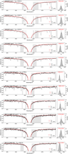 |
Fig. A.3 Similar to Fig. A.2 but for stars with direct IRFM measurements. |
| In the text | |
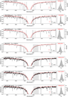 |
Fig. A.4 Similar to Fig. A.2 but for stars with asteroseismic measurements. |
| In the text | |
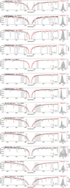 |
Fig. A.5 Similar to Fig. A.2 but for other giant stars. |
| In the text | |
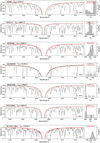 |
Fig. A.6 Similar to Fig. A.2 but for CEMP stars. |
| In the text | |
 |
Fig. A.7 A(Mg) offsets induced by a −50 K Teff offset when derived from the line at 5711 Å. The horizontal line represents no offset. ‘X’ represents the element Mg in this case. |
| In the text | |
Current usage metrics show cumulative count of Article Views (full-text article views including HTML views, PDF and ePub downloads, according to the available data) and Abstracts Views on Vision4Press platform.
Data correspond to usage on the plateform after 2015. The current usage metrics is available 48-96 hours after online publication and is updated daily on week days.
Initial download of the metrics may take a while.


![$\left[ {{{\rm{A}} \mathord{\left/ {\vphantom {{\rm{A}} {\rm{B}}}} \right. \kern-\nulldelimiterspace} {\rm{B}}}} \right] = \log {\left( {{{N\left( {\rm{A}} \right)} \over {N\left( {\rm{B}} \right)}}} \right)_{{\rm{Star}}}} - \log {\left( {{{N\left( {\rm{A}} \right)} \over {N\left( {\rm{B}} \right)}}} \right)_{{\rm{Sun}}}}$](/articles/aa/full_html/2023/11/aa47208-23/aa47208-23-eq63.png)