| Issue |
A&A
Volume 699, July 2025
|
|
|---|---|---|
| Article Number | A32 | |
| Number of page(s) | 26 | |
| Section | Catalogs and data | |
| DOI | https://doi.org/10.1051/0004-6361/202554228 | |
| Published online | 01 July 2025 | |
Large databases of metal-poor stars corrected for three-dimensional and/or non-local thermodynamic equilibrium effects
1
Dipartimento di Fisica e Astronomia, Università degli Studi di Firenze,
Via G. Sansone 1,
50019
Sesto Fiorentino,
Italy
2
INAF/Osservatorio Astrofisico di Arcetri,
Largo E. Fermi 5,
I-50125
Firenze,
Italy
★ Corresponding author: This email address is being protected from spambots. You need JavaScript enabled to view it.
Received:
22
February
2025
Accepted:
2
May
2025
Abstract
Early chemical enrichment processes can be revealed by the careful study of metal-poor stars. In our Local Group, we can obtain spectra of individual stars to measure their precise, but not always accurate, chemical abundances. Unfortunately, stellar abundances are typically estimated under the simplistic assumption of local thermodynamic equilibrium (LTE). This can systematically alter both the abundance patterns of individual stars and the global trends of chemical enrichment. The SAGA database compiles the largest catalogue of metal-poor stars in the Milky Way. For the first time, we provide the community with the SAGA catalogue fully corrected for non-LTE (NLTE) effects, using state-of-the-art publicly available grids. In addition, we present an easy-to-use online tool NLiTE that quickly provides NLTE corrections for large stellar samples. For further scientific exploration, NLiTE facilitates the comparison of different NLTE grids to investigate their intrinsic uncertainties. Finally, we compare the NLTE-SAGA catalogue with our cosmological galaxy formation and chemical evolution model, NEFERTITI. By accounting for NLTE effects, we can solve the long-standing discrepancy between models and observations in the abundance ratio of [C/Fe], which is the best tracer of the first stellar populations. At low [Fe/H] < −3.5, models are unable to reproduce the high measured [C/Fe] in LTE, which are lowered in NLTE, aligning with simulations. Other elements are a mixed bag, where some show improved agreement with the models (e.g. Na) and others appear even worse (e.g. Co). Few elemental ratios do not change significantly (e.g. [Mg/Fe], [Ca/Fe]). Properly accounting for NLTE effects is fundamental for correctly interpreting the chemical abundances of metal-poor stars. Our new NLiTE tool, thus, enables a meaningful comparison of stellar samples with chemical and stellar evolution models as well as with low-metallicity gaseous environments at higher redshift.
Key words: catalogs / stars: abundances / stars: atmospheres / Galaxy: abundances / Galaxy: evolution
© The Authors 2025
 Open Access article, published by EDP Sciences, under the terms of the Creative Commons Attribution License (https://creativecommons.org/licenses/by/4.0), which permits unrestricted use, distribution, and reproduction in any medium, provided the original work is properly cited.
This article is published in open access under the Subscribe to Open model. This email address is being protected from spambots. You need JavaScript enabled to view it. to support open access publication.
1 Introduction
Metal-poor (MP) stars ([Fe/H] < −1; Beers & Christlieb 2005) are ancient relics of the early chemical enrichment in the Universe, providing a unique window into the conditions and processes that shaped the formation of the first stellar populations (e.g. Tumlinson 2007; Salvadori et al. 2007; Hartwig et al. 2015; Sarmento et al. 2018; Koutsouridou et al. 2024). These stars, observed today in our Local Group, retain in their photospheres the chemical signatures of the gas clouds from which they formed. Unravelling their detailed and accurate elemental abundances is therefore key to answering numerous scientific questions. In particular, MP stars provide valuable insights into the nature of the first metal-free Population III (Pop III) stars (their masses, supernova explosion energies, rotation rates, and mixing processes), and into the transition to normal Population II (Pop II) star formation (e.g. de Bennassuti et al. 2017; Ishigaki et al. 2018; Hartwig et al. 2019; Vanni et al. 2023; Koutsouridou et al. 2023; Sestito et al. 2024). They can be used to test theoretical predictions of Big Bang nucleosynthesis (e.g. the lithium problem; see Fields 2011), stellar nucleosynthesis and galactic chemical evolution models (e.g. Matteucci et al. 2021; Rossi et al. 2024a; Brauer et al. 2025).
In addition, when paired with kinematic data, MP stars can offer a unique perspective on the accretion and early formation history of the Milky Way and its satellite galaxies (e.g. Gaia Collaboration 2018a,b).
However, confirming stellar candidates as very metal poor (VMP, [Fe/H] < −2) or extremely metal poor (EMP, [Fe/H] < −3) requires medium- to high-resolution spectroscopic follow-up observations, which are resource intensive. Consequently, the number of confirmed VMP stars remains significantly lower than the available candidate pool (e.g. Xylakis-Dornbusch et al. 2022; Martin et al. 2024). Databases such as the Stellar Abundances for Galactic Archaeology (SAGA)1 compile such follow-up data, currently including thousands of MP stars observed at high or medium resolution (Suda et al. 2008, 2011; Yamada et al. 2013; Suda et al. 2017).
Almost all of the stars in the SAGA database have chemical abundances determined using one-dimensional (1D) model atmospheres and the assumption of local thermodynamic equilibrium (LTE). In many cases, the basic atmospheric stellar parameters, such as the effective temperature, Teff; surface gravity, log g; and micro-turbulence velocity, vturb, are also determined spectroscopically within the LTE framework. The LTE assumption is generally valid when frequent particle collisions maintain a Maxwellian velocity distribution in the system, such that the energy level populations are determined solely by the local temperature and electron density, as dictated by the Saha and Boltzmann equations. However, in realistic stellar atmospheres the gas density is low, collisions between particles are rare, and radiative processes – absorption, emission, and scattering of photons – play a dominant role in determining the energy level populations, causing departures from equilibrium. These non-LTE (NLTE) effects can significantly affect the derived chemical abundances, with discrepancies ranging from negligible to over an order of magnitude, depending on the stellar atmospheric conditions and the spectral line analysed (e.g. Asplund 2005; Mashonkina 2014; Amarsi et al. 2020; Lind et al. 2022; Lind & Amarsi 2024). The problem is compounded at low metallicities, where NLTE effects become progressively stronger due to the decreased collisional rates and increased radiative rates caused by low ultraviolet (UV) opacity (e.g. Mashonkina et al. 2023; Shi et al. 2025). These metallicity-dependent NLTE effects, can create artificial abundance trends with metallicity in the LTE assumption, potentially distorting our understanding of early chemical evolution.
Additionally, 1D atmosphere models, which assume static and homogeneous layers, overlook dynamic 3D phenomena, for example stellar granulation caused by convection. These processes create temperature and density inhomogeneities that impact spectral line formation, often in a direction opposite to NLTE effects (e.g. Asplund 2005). Moreover, 3D and NLTE effects are non-linearly coupled, and therefore only models that account simultaneously for the two effects can provide highly accurate and reliable abundance determinations (Lind & Amarsi 2024). Accurate chemical abundances, taking into account 3D and/or NLTE effects, are therefore fundamental so that the stellar observations can be contrasted against models in a meaningful way (e.g. Cayrel et al. 2004; Kobayashi et al. 2020; Skúladóttir et al. 2024a; Storm et al. 2025) and can be compared to higher-redshift observations of gaseous absorbers, which do not undergo the same effects (e.g. Cooke et al. 2011; Skúladóttir et al. 2018; Welsh et al. 2022; Saccardi et al. 2023; Vanni et al. 2024).
To address these challenges, much effort has been put in the development of sophisticated 1D and 3D NLTE models, including high-quality model atoms, atmospheres and spectral synthesis techniques (for more details see the comprehensive reviews by Asplund 2005 and Lind & Amarsi 2024, and references therein). Currently, 1D NLTE abundance corrections for specific spectral lines as a function of atmospheric parameters (Teff, log g, [Fe/H] and in cases vturb, [X/Fe] or line equivalent width) are readily available on the following websites:
MPIA2 for lines of O I, Mg I, Si I, Ca I-II, Ti I-II, Cr I, Mn I, Fe I-II, and Co I
INASAN3 for lines of Na I, Mg I, Ca I and Ca II, Ti II, Fe I, Zn I-II, Sr II, Ba II and Eu II
INSPECT4 for lines of Li I, O I, Na I, Mg I, Ti I, Fe I-II, Sr II In addition, various grids of 1D NLTE corrections for individual elements are available in the literature (e.g. Takeda et al. 2005; Korotin et al. 2015; Nordlander & Lind 2017). Due to the large computational cost involved, grids of 3D NLTE corrections are currently available only for a few chemical species and in most cases a limited range of stellar parameters (e.g. Sbordone et al. 2010; Amarsi et al. 2019, 2022; Gallagher et al. 2020).
Although a plethora of studies have corrected the abundances of various stellar samples for one or more chemical elements (e.g. Andrievsky et al. 2007, 2008, 2009, 2010; Zhao et al. 2016; Mashonkina et al. 2017a, 2019b; Kovalev et al. 2019; Mashonkina & Romanovskaya 2022; Shen et al. 2023), a unified catalogue encompassing a large sample of NLTE-corrected abundances for MP stars, extending down to the lowest metallicities, is still missing. As a result, theoretical predictions are commonly compared with uncorrected datasets, such as the SAGA database (Hartwig et al. 2018; Kobayashi et al. 2020; Koutsouridou et al. 2023; Vanni et al. 2023; Rossi et al. 2024b). This practice can lead to flawed conclusions regarding stellar nucleosynthesis, galactic chemical evolution, and the properties of the first stars.
In this work, our aim is to apply NLTE corrections to the entire SAGA catalogue of Galactic MP stars by utilizing all available NLTE grids. The main challenge with this endeavour is that SAGA does not include chemical abundance measurements for specific spectral lines, which are necessary for calculating precise and accurate NLTE corrections. To tackle this, we identified the most commonly observed spectral lines for each element, as a function of stellar atmospheric parameters (Teff, log g, [Fe/H] and in cases [X/Fe]), and computed average NLTE corrections for these lines from the available grids. While these corrections are approximate – due to differences in the lines used across observational studies and the fact that NLTE grids are sometimes available only for a subset of the lines commonly used by observers – they are statistically robust and provide a reliable representation of general NLTE effects. Thus, they are adequate for analysing large datasets to be compared with theoretical chemical evolution models.
Currently, SAGA is the largest available catalogue for chemical abundances of MP stars, but this is likely to change in the near future with the large ongoing and upcoming spectroscopic surveys, such as GALAH, LAMOST, WEAVE and 4MOST (Martell et al. 2017; Zhao et al. 2012; Jin et al. 2024; de Jong et al. 2019). Some of these surveys (GALAH, 4MOST) are aiming to release state-of-the-art NLTE abundances for all chemical elements, while other surveys might mainly rely on the LTE approach. Thus, the need is evident for an efficient tool to easily correct large stellar databases for NLTE effects. As part of this effort, we have therefore developed the online tool NLiTE, which is optimized for MP stars analysed through optical spectra. The tool interpolates within precomputed average NLTE grids to provide corrections given the atmospheric parameters of each individual star. It is particularly useful for quickly providing NLTE-corrections for large stellar samples and/or when the information about individual spectral lines is unavailable. Furthermore, NLiTE facilitates direct comparisons between different NLTE studies, as it includes multiple NLTE grids for the same element where available.
With this work, we therefore provide the astronomic community with a full NLTE-corrected SAGA catalogue of MP stars (online Table 2), as well as the NLiTE tool5 to easily correct large databases and to compare different studies of NLTE effects. Finally, we compare this new NLTE SAGA database with the predictions of our cosmological galaxy formation model of the Milky Way halo, NEFERTITI (Koutsouridou et al. 2023). Thus, we show the importance of using accurate chemical abundances when trying to understand early chemical enrichment and the properties of the first stars in the Universe.
2 The NLiTE online tool
We present the online tool NLiTE, designed to provide NLTE abundance corrections for MP stars, which have been analysed using optical spectra (3500 Å ≲ λ ≲ 10 000 Å). The main goals of this tool are: (a) Construct a fully corrected NLTE-SAGA database (Sect. 4) to contrast against models (Sect. 5); (b) Provide an easy way to compare different grids of NLTE corrections, and establish which elemental ratios [X/Fe] are the least or most affected; (c) Have a readily available tool for the community to use and correct large databases of MP stars. For the public use, two modes of NLiTE are available: (1) Correcting a single element with a grid of choice; or (2) Correcting all elements using our fiducial grids (Table A.1). Both modes include the option to receive a ready-to-use bib file, to facilitate and encourage citations to the original NLTE grids.
By interpolating within precomputed grids, NLiTE computes corrections based on given stellar atmospheric parameters: Teff, log g, [Fe/H], and either [Element/Fe] or [Element/H]. Unlike other tools, NLiTE does not take spectral line data as input. The precomputed grids are built from publicly available NLTE datasets (Sect. 2.2) that are originally tied to specific spectral lines. These grids are averaged using the corrections of the lines most representative of MP stars at given atmospheric conditions. As a result, while NLiTE provides approximate corrections, it can be particularly useful for analysing large stellar samples or when equivalent width measurements are unavailable. Furthermore, by incorporating multiple grids per element when available, NLiTE facilitates direct comparisons between NLTE corrections from different studies.
Line list.
2.1 Line lists
For each element, we assume a line list that is the intersection between the lines most frequently used in the chemical abundance analysis of MP stars and those for which NLTE corrections exist. The selection of the commonly used lines is largely based on the studies of Fulbright (2000); Cayrel et al. (2004); Barklem et al. (2005); Ishigaki et al. (2012); Cohen et al. (2013); Roederer et al. (2014); Jacobson et al. (2015); Sakari et al. (2018); and Li et al. (2022). Among these, we select the lines with available NLTE corrections. In cases where multiple NLTE grids are available for the same element, we choose when possible to adopt lines that are common across all grids. This allows a direct comparison between the published NLTE grids, which is presented in Sect. 3, and in Appendix B. Our analysis shows that in most cases, the NLTE corrections of different lines (at given stellar parameters) are in good agreement, with standard deviation σ ≲ 0.1 dex (see Sect. 4.3). This indicates that our adopted line list is a reliable way to calculate NLTE corrections for large samples, since in general these are not strongly dependent on the exact line list. The adopted line list is published in an online Table 1.
Depending on the set of stellar parameters (Teff, log g, [Fe/H], and [X/H]), certain lines may be very weak (making them challenging to measure) or severely saturated (making them less sensitive to abundance) and are, thus, commonly discarded in observational studies. To account for this, for each stellar parameter set we compute the average NLTE correction using only lines with predicted equivalent widths (EW) in the range 5 mÅ < EW < 200 mÅ. Exceptions to this are elements that have only a few lines available, which are therefore rarely discarded. Thus, we put no upper limit on the EW for: Li, Al, Na, K, Sr, and Ba.
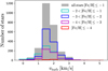 |
Fig. 1 All MP SAGA stars with microturbulence velocity, vturb, estimates in different metallicity bins. In the case of multiple entries from different surveys and/or authors for the same star, the microturbulence and [Fe/H] here are equal to the mean values. |
2.2 NLTE grids
The NLTE grids are adopted from the literature, in particular from the databases of MPIA6, INASAN, INSPECT, that of Anish M. Amarsi7, as well as individual studies for specific elements (Table A.1). For each element X, the grids are given as a function of Teff, log g, [Fe/H], and in some cases elemental abundance [X/H]. The range of the parameter space for each grid is given in Table A.1.
Through NLiTE we facilitate the use of all available grids for individual elements. However, for our NLTE-SAGA database we choose a fiducial grid for each element, as listed in Table A.1. Since our final goal is to be able to correct large databases with stars in various evolutionary phases, we typically adopt as our fiducial grids those that cover the largest parameter space.
2.3 Impact of microturbulence
Several NLTE grids include microturbulent velocity, vturb, as an input parameter. By inspecting the distribution of vturb in all the observed metal-poor MW stars in the SAGA database (Fig. 1), we find that it peaks at vturb = 1.5 km/s in all metallicity bins, except from the lowest one, [Fe/H] ≤ −4 where it peaks at vturb = 2 km/s. But these stars represent only ~1% of the total MP population.
To assess the impact of vturb on the NLTE corrections, we investigate three representative stars at [Fe/H] = −2: (i) Teff = 4500 K, log g = 1.5; (ii) Teff = 5000 K, log g = 2.0; and (iii) Teff = 6000 K, log g = 4.0. Fig. 2 compares the mean NLTE corrections (averaged across all spectral lines considered; see Table 1) as a function of vturb, ranging from 0–3 km/s, to the case where the most common vturb = 1.5 km/s is assumed. The results are based on our fiducial grids for each element (see Table A.1) and the assumed abundance ratios correspond to typical MW values at this metallicity: [C/Fe] = 0, [O/Fe] + 0.6, [Na/Fe] = 0, [Mg/Fe] = +0.4, [Al/Fe] = −0.5, and [Si/Fe] = +0.5. It should be noted that not all grids offer the full range of 0–3 km/s. Furthermore, the elements Li I, Ca I, Zn I, Sr II, Ba II, and Eu II are missing because Wang et al. (2021) and the INASAN database do not include vturb as an input parameter. Similarly, Norris & Yong (2019) do not account for vturb in their corrections of CH.
Fig. 2 shows that our fiducial NLTE corrections do not depend strongly on vturb. In all cases, the deviations from the standard vturb = 1.5 km/s case remain within 0.03 dex. Therefore we adopt this fixed value as a standard in our NLTE grids whenever vturb is an input parameter. Further discussion on other NLTE grids and broader parameter sets can be found in the respective sections for each element (Sect. 3).
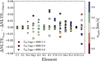 |
Fig. 2 Difference in NLTE corrections, when assuming vturb = 0, 0.5, 1, 2 and 3 km/s, compared to the most common value for MP SAGA stars, vturb = 1.5 km/s. Three representative stellar model atmospheres at [Fe/H] = −2 are shown (circles, squares, triangles). |
2.4 Interpolation-extrapolation
For each element and corresponding set of NLTE corrections (see Table A.1) we construct an interpolation function in a three- or four-dimensional space (Teff, log g, [Fe/H] and when available [X/Fe] or A(X)), using the linear scipy.interpolate.Rbf function in Python.
We note that, for stellar parameters within each ΔNLTE grid, the scipy multiquadric fitting function gives corrections that differ less than 0.1 dex from those obtained with the linear method. For stellar parameters outside the grids, the differences tend to be larger. Therefore, rather than extrapolating beyond the available grids, NLiTE applies the NLTE corrections corresponding to the nearest grid boundary.
3 NLTE grids for individual elements
3.1 Lithium I
We computed NLTE corrections for the Li I resonance line at 670.7 nm adopting the grids from Lind et al. (2009), Sbordone et al. (2010) and Wang et al. (2021) (see Fig. 3).
The Lind et al. (2009) corrections were derived using 1D-model atmospheres, and are available for vturb = 1, 2 and 5 km/s. We adopted the average between the vturb = 1 and vturb = 2 km/s corrections, noting that their differences do not exceed 0.1 dex, at fixed Teff, log g and [Fe/H].
Sbordone et al. (2010) computed corrections for both 1D- and 3D-hydrodynamical model atmospheres and provided analytical fits of A(Li)3D,NLTE, A(Li)1D,NLTE and A(Li)3D,NLTE as functions of equivalent width, Teff, log g, and [Fe/H] but restricted only to dwarf stars. In the overlapping parameter space, we find that the 1D NLTE corrections from Sbordone et al. (2010) are weaker than those of Lind et al. (2009), which are more negative by approximately 0.05 dex. The 3D NLTE corrections of Sbordone et al. (2010) are slightly positive, about 0.03 dex higher than their 1D values, in accordance with previous studies who reported <0.1 dex differences in lithium abundance between 3D NLTE and 1D NLTE (Asplund et al. 2003; Barklem et al. 2003).
Wang et al. (2021) provided 3D NLTE corrections covering a broader parameter range along with an interpolation routine8 based on multilayer perceptrons (a class of fully connected feed-forward neural networks), which we used to construct our NLTE grid. We note that using our linear interpolation method, we find corrections for individual stars that differ by no more than 0.018 dex from those obtained with Wang et al. (2021)’s interpolation routine.
The Wang et al. (2021) corrections are generally more negative than those of Lind et al. (2009) by approximately 0.1 dex at Teff ≤ 4500 K. At higher Teff, this trend reverses. Compared to the 3D corrections from Sbordone et al. (2010), the Wang et al. (2021) values are, on average, about 0.05 dex more negative. These differences may arise from a NLTE effect identified by Wang et al. (2021) that was previously overlooked, involving the blocking of UV lithium lines by background opacities.
Overall, the NLTE corrections span the range [−1.1, +0.45] dex (not all values are shown in Fig. 3) and tend to be more positive at lower A(Li) values in all grids. Given the broader parameter coverage of Wang et al. (2021), we adopt this as our fiducial grid.
Mott et al. (2020) computed also 1D and 3D NLTE A(Li) abundance corrections. We did not incorporate those here, as the authors provide their own Python script that evaluates them as a function of Teff, log g, [Fe/H], lithium isotopic ratio 6Li/7Li and A(Li)9. However, we note that their 1D corrections are typically 0.02 dex lower than their 3D counterparts, with the latter being, on average, 0.06 dex more positive than those of Wang et al. (2021).
Finally, Shi et al. (2007) reported 1D NLTE abundances for Li in 19 stars with −2.5 < [Fe/H] < −1, and 3 < log g < 5. Their corrections are small, 0 < |Δ1D NLTE| < 0.03, for the majority of the sample, and generally in good agreement with those of Sbordone et al. (2010), while Lind et al. (2009) and Wang et al. (2021) present slightly stronger negative corrections. However, the work of Shi et al. (2007) does not include a grid of corrections, and is thus not implemented here.
3.2 Molecular carbon (CH)
Due to complexities in modelling molecular spectra, which involve numerous energy levels and lines, a full grid of NLTE corrections for the molecular CH G-band is not currently available. We, therefore, adopted the empirical CH corrections from Norris & Yong (2019), who considered the analysis of near-infrared high-excitation C I lines in metal-poor stars, to assess the role of NLTE effects in determining A(C)3D,NLTE values from G-band data.
The authors, initially, compiled 9 (−5.7 ≤ [Fe/H] ≤ −1) stars with existing 3D-1D LTE CH corrections (Collet et al. 2006, 2007, 2018; Frebel et al. 2008; Spite et al. 2013; Gallagher et al. 2016) and computed the linear least-squares best fit to the data:
![Mathematical equation: $\[\mathrm{A}(\mathrm{CH})_{3 \mathrm{D}, \mathrm{LTE}}=\mathrm{A}(\mathrm{CH})_{1 \mathrm{D}, \mathrm{LTE}}+0.087+0.170[\mathrm{Fe} / \mathrm{H}]_{1 \mathrm{D}, \mathrm{LTE}}.\]$](/articles/aa/full_html/2025/07/aa54228-25/aa54228-25-eq1.png) (1)
(1)
They then determined A(CH)1D,LTE abundances for 23 stars (dwarfs and subgiants) using high-resolution, high signal-to-noise spectra from the literature, with A(CI)1D,NLTE abundances previously provided by Fabbian et al. (2009b). Using Equation (1), they converted A(CH)1D,LTE to A(CH)3D,LTE abundances, and noted that 3D corrections to A(CI)1D,NLTE are likely insignificant, as indicated by Fabbian et al. (2009b) and Dobrovolskas et al. (2013). By requiring that A(CH)3D,NLTE = A(CI)3D,NLTE, they found the best linear fit for [Fe/H] > −3:
![Mathematical equation: $\[\mathrm{A}(\mathrm{CH})_{3 \mathrm{D}, \mathrm{NLTE}}=\mathrm{A}(\mathrm{CH})_{3 \mathrm{D}, \mathrm{LTE}}+0.483+0.240[\mathrm{Fe} / \mathrm{H}]_{1 \mathrm{D}, \mathrm{LTE}}.\]$](/articles/aa/full_html/2025/07/aa54228-25/aa54228-25-eq2.png) (2)
(2)
For lower metallicities, where CH features and C I lines are weak, the authors made the conservative assumption that A(CI)3D,NLTE = A(CH)3D,LTE, and hence:
![Mathematical equation: $\[\mathrm{A}(\mathrm{CH})_{3 \mathrm{D}, \mathrm{NLTE}}=\mathrm{A}(\mathrm{CH})_{3 \mathrm{D}, \mathrm{LTE}}.\]$](/articles/aa/full_html/2025/07/aa54228-25/aa54228-25-eq3.png) (3)
(3)
The above equations imply that strong negative corrections should be applied to the observed A(CH)1D,LTE abundances for stars with [Fe/H] ≲ −1.4, reaching ~−0.9 dex at [Fe/H] = −6.
Recently, Popa et al. (2023) made the first attempt at computing the G band of the CH molecule in NLTE for a cool stellar atmosphere typical of red giants (log g = 2.0, Teff = 4500 K). Their results showed that A(C)1D,NLTE-A(C)1D,LTE corrections are consistently positive and increasing towards lower [Fe/H] and [C/Fe]. However, these findings are subject to significant uncertainties, since molecular collisional data are still poorly constrained (Lind & Amarsi 2024). Furthermore, Popa et al. (2023) acknowledged that their analysis, based on 1D hydrostatic models, neglects time-dependent 3D phenomena such as convection and turbulence, that have been shown to lower CH abundances at least in LTE (see above). Therefore, it remains unclear whether accounting for 3D effects will overcompensate for the positive 1D NLTE – 1D LTE corrections, resulting in the net negative corrections suggested by Norris & Yong (2019).
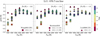 |
Fig. 3 NLTE corrections for Li I, colour-coded by log g: squares are from Wang et al. (2021), triangles from Lind et al. (2009) and circles from Sbordone et al. (2010). Three metallicities are shown: [Fe/H] = −3 (left), [Fe/H] = −2 (middle), and [Fe/H] = −1 (right). |
3.3 Carbon I and oxygen I
We include grids for the 3D NLTE corrections of C I and O I from Amarsi et al. (2019), in the provided range of 5000 K ≤ Teff ≤ 6500 K, 3 ≤ log g ≤ 5, and −3 ≤ [Fe/H] ≤ 0. In addition, we provide the grid for their 1D NLTE corrections for C I and O I, in the range 4000 K ≤ Teff ≤ 7500 K, 0 ≤ log g ≤ 5, −5 ≤ [Fe/H] ≤ 0 and −0.4 ≤ [X/Fe] ≤ 1.2. We used three infrared lines for C I, 909.5, 911.1 and 940.6 nm, which are still visible in extremely metal-poor stars and the O I triplet at 777 nm. Since EWs were not provided, corrections were included for all three lines for the entire grid, both for C I and O I.
The comparison between the 1D NLTE and 3D NLTE results of Amarsi et al. (2019) are shown in Figs. B.1 and B.2. In addition, we computed the mean 1D NLTE corrections from Bergemann et al. (2021) for the O I 777 nm triplet, which we find to be in general ~0.1–0.3 dex weaker than those of Amarsi et al. (2019; see Fig. B.2). Here we adopt the corrections from Amarsi et al. (2019) as our fiducial O I grid, as it has a larger range in [Fe/H] compared to that of Bergemann et al. (2021).
The work of Spite et al. (2013) calculated 3D NLTE corrections for CI lines in two stars at [Fe/H] = −3.3, Teff ≈ 6200 K, and log g = 4.0. They find corrections of Δ3D NLTE = −0.45 dex for both stars, while the Amarsi corrections for these stars are less strong, Δ3D NLTE ≲ −0.2 dex. Other works that have computed 1D NLTE corrections for C I lines include Takeda & Honda (2005); Fabbian et al. (2006), and Alexeeva & Mashonkina (2015). The results of these three papers were compared in Alexeeva & Mashonkina (2015, their Fig. 5) for a test case of Teff = 6000 K and log g = 4. Comparable results were found at [Fe/H] ≳ −1, but significantly smaller corrections at [Fe/H] ≲ −2, compared to the older works. For this specific test case at low metallicities, the work of Amarsi et al. (2019) is generally in agreement with that of Alexeeva & Mashonkina (2015), within ≈ 0.05 dex. None of these aforementioned works (Takeda & Honda 2005; Fabbian et al. 2006; Alexeeva & Mashonkina 2015; Spite et al. 2013) provide full 1D NLTE C I correction grids, and are therefore not included in our selected grids.
In regards to O I, Takeda (2003) calculated 1D NLTE corrections for a sample of Milky Way disk and halo stars (late-F through early-K types). They found a typical correction of Δ1D NLTE = −0.1 dex for their stellar sample at [Fe/H] < −1. This is comparable to the 1D NLTE results of Amarsi et al. (2019) for similar stars, agreeing within ≈ 0.05 dex. Sitnova & Mashonkina (2018) found slightly lower corrections at [Fe/H] < −1, Δ1D NLTE ≈ −0.05 dex, deviating by ≈ 0.1 dex from Amarsi et al. (2019). The 1D NLTE corrections for O I as calculated by Fabbian et al. (2009a), on the other hand, are stronger than those of Amarsi et al. (2019), with differences up to ≈ 0.4 dex at the lowest [Fe/H] (as seen by Fig. 7 in Fabbian et al. 2009a). As far as we are aware, the grids of Takeda (2003), Fabbian et al. (2009a) and Sitnova & Mashonkina (2018) are not available publicly, and are therefore not included in this work.
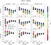 |
Fig. 4 NLTE corrections for Na I, colour-coded by log g: squares are from Lind et al. (2011), triangles from Alexeeva et al. (2014), and circles from Lind et al. (2022). The rows show three metallicities: [Fe/H] = −2 (top), [Fe/H] = −3 (middle), and [Fe/H] = −4 (bottom). The columns show different [Na/Fe] LTE values: [Na/Fe] = −0.6 (left), [Na/Fe] = 0 (middle) and [Na/Fe] = +0.6 (right). The symbols are hatched diagonally in cases where only one line is available (i.e. EW > 5 mÅ). The error bars represent the standard deviation of the NLTE corrections of the different Na I lines at a given set of stellar parameters. |
3.4 Molecular nitrogen (CN)
In metal-poor stars, nitrogen is most commonly measured through the CN molecular bands, and less frequently through NH lines. Calculating NLTE grids for molecular bands is computationally expensive and complex. Furthermore, 3D effects are likely to be significant, since molecular lines are typically very sensitive to temperature. Finally, when N is measured through CN, the accurate abundance for C is also crucial, which is non-trivial to obtain, see the previous subsections. In the absence of a NLTE grid for CN, we include only [N/Fe]LTE in our fiducial SAGA catalogue, marked specifically to indicate that this is a LTE result.
3.5 Sodium I
We computed NLTE corrections for the Na I doublets at 5682/5688 Å and 5889/5895 Å employing the grids of Lind et al. (2011), Alexeeva et al. (2014) and Lind et al. (2022) (see Fig. 4). The Lind et al. (2022) corrections are available for vturb = 1 and 2 km/s, with the differences between them remaining below 0.13 dex across all lines and stellar parameters. We adopted the average of the two.
The two Na doublets are known to have significantly different NLTE corrections (e.g. Lind et al. 2022). Therefore, applying a single mean correction across both could lead to inaccurate Na abundances, in cases where only one doublet is observed. To avoid this, we divided SAGA stars into three groups: those with Na abundances based on the resonance lines at 5889/5895 Å, those based on the subordinate lines at 5682/5688 Å and those observed using both doublets. For each group, we applied the mean correction of the corresponding lines. For SAGA stars with no information on the Na lines used, we applied the mean corrections of all four lines, which are shown in Fig. 4. All three versions of the grids are available in NLiTE.
The mean corrections are predominantly negative, reaching ~−0.7 dex (~−0.4 dex and −1 dex for the subordinate and resonance lines, respectively), except at the lowest metallicities, where a slight, positive upturn is found. As seen in Fig. 4, at [Fe/H] = −3 and [Fe/H] = −2, the corrections are generally more negative at higher temperatures and lower surface gravities. However, these trends appear to reverse at the lowest metallicity bin.
Overall the agreement between the different works is quite good, differing by ≲0.1 dex in most cases. Yet, in some parts of the parameter space, the differences between different grids can reach ~0.3 dex (see also Sect. 4.4). As our fiducial grid we choose that of Lind et al. (2022) since it covers the largest parameter space.
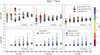 |
Fig. 5 NLTE corrections for Mg I, colour-coded by log g: stars are from Bergemann et al. (2017), squares are from Mashonkina (2013), triangles from Osorio & Barklem (2016), and circles from Matsuno et al. (2024). The top row compares the corrections of Osorio & Barklem (2016) assuming the same EWs as given by Bergemann et al. (2017) and Mashonkina (2013) for each Mg I line, at fixed Teff, log g and [Fe/H] values. The bottom row compares Osorio & Barklem (2016) to the 1D and 3D NLTE corrections of Matsuno et al. (2024), only available for dwarf stars, for A(Mg)=7. The error bars represent the standard deviation of different Mg I lines (often smaller than the depicted symbols); the hatched symbols indicate corrections that are based only on one line. |
3.6 Magnesium I
We computed mean corrections for seven optical Mg I lines, using the grids of Merle et al. (2011), Mashonkina (2013), Bergemann et al. (2017), Osorio & Barklem (2016), Lind et al. (2022) and Matsuno et al. (2024) (see Fig. 5). The last three grids are given as a function of abundance A(Mg), while [Mg/Fe] = +0.4 is adopted for metal-poor stars in the grids of Merle et al. (2011) and Mashonkina (2013). By computing the Osorio & Barklem (2016) corrections for the same EWs as given by Mashonkina (2013) and Bergemann et al. (2017) at each Teff, log g and [Fe/H], we see that the three grids are in remarkable agreement (top panels of Fig. 5). The same is true for the corrections of Lind et al. (2022), which are not displayed in Fig. 5 to avoid overcrowding the figure. ΔNLTE are predominantly positive and increase with decreasing log g and metallicity. The scatter in the corrections of the different lines is in most cases small, σ < 0.1.
Recently, Matsuno et al. (2024) computed both 1D- and 3D NLTE corrections for FG-type dwarfs. Their 1D corrections are similar to those of Osorio & Barklem (2016; bottom panels of Fig. 5), while those assuming 3D are typically higher by 0.1–0.2 dex (the difference ΔNLTE3D − ΔNLTE1D ranges between −0.08 and +0.3 approximately). We note that the 3D corrections of Matsuno et al. (2024) show a much stronger dependence on vturb than their own 1D corrections, or those of Osorio & Barklem (2016; see Sect. 2.3). Specifically, the differences between vturb = 1 km/s vturb = 2 km/s reach up to 0.14 dex in 3D, compared to just 0.016 dex in 1D. Similarly, their 3D corrections exhibit significantly larger line-to-line scatter, with the standard deviation reaching σ = 0.36 dex, in comparison to 0.07 dex for their 1D corrections and 0.045 dex for those of Osorio & Barklem (2016).
We adopt the grid from Osorio & Barklem (2016) as default because it spans the broadest parameter range and includes an additional dependence on A(Mg).
3.7 Aluminium I
Nordlander & Lind (2017) and Lind et al. (2022) have provided grids of EWs for several Al lines, as a function of Teff, log g, [Fe/H] and [Al/Fe], computed in LTE and NLTE. We derived the NLTE correction for each line by interpolating LTE equivalent widths onto the NLTE curves of growth. The Lind et al. (2022) corrections are given for vturb = 1 and 2 km/s; we adopted their average, noting that the differences between them do not exceed 0.08 dex when applied to all MP SAGA stars. They are based on 1D model atmospheres, while Nordlander & Lind (2017) also provide values for temporally and spatially averaged ⟨3D⟩ hydrodynamical models.
For each stellar parameter set, we computed the mean NLTE correction of the Al resonance lines at 3944 Å and 3961 Å, which are used in the vast majority of MP stars. The resulting ΔNLTE values are shown in Fig. 6, alongside 1D corrections for individual stars by Baumueller & Gehren (1997). In addition, we computed mean corrections for the Al subordinate lines at 6696–8773 Å, which are often used at [Fe/H] ≳ −1.5, where the resonance lines become too strong. Both sets of NLTE grids are provided in NLiTE. SAGA stars were categorized based on whether their Al abundances were derived from resonance or subordinate lines, and the corresponding corrections were applied accordingly.
The resonance lines corrections are predominantly positive and tend to increase with decreasing log g and increasing Teff (Fig. 6). The same trend is seen in the subordinate lines (not shown here) which however exhibit weaker corrections (see also Fig. 11). The behavior of ΔNLTE with [Al/Fe] is not monotonous but depends on the specific stellar parameters. We adopt the grid from Lind et al. (2022) as our reference, as it covers the largest [Fe/H] range.
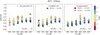 |
Fig. 6 Mean NLTE corrections of the resonance Al I lines at 3944 Å and 3961 Å, colour-coded by log g: triangles are from Lind et al. (2022) and circles from Nordlander & Lind (2017). The corrections for individual stars from Baumueller & Gehren (1997) are shown with crosses (X), for four test cases of Teff = 5200, 5500, 5780, and 6500 K; and log g=4.50, 3.50, 4.44, and 4.00. The error bars represent the standard deviation of the corrections of the two lines (often smaller than the depicted symbols). The hatched symbols indicate corrections that are based on one line. |
3.8 Silicon I
In total, eight optical lines of Si I were used for our average NLTE corrections, using the grids of Bergemann et al. (2013) and Amarsi & Asplund (2017) (see Fig. B.3). The Amarsi & Asplund (2017) corrections are provided for vturb = 1 and 2 km/s. We adopted the average of the two, noting that their difference remains below 0.05 dex for 99.4% of MP SAGA stars (with a maximum difference of 0.22 dex).
We find that the mean corrections are mostly positive and tend to increase with increasing Teff, decreasing log g, and decreasing [Si/Fe]. The Amarsi & Asplund (2017) corrections are significantly larger than those of Bergemann et al. (2013) at high Teff, with the latter being in most cases close to zero at [Fe/H] ≥ −3. We adopt the corrections of Amarsi & Asplund (2017) as default because they are given as a function of [Si/Fe], in addition to Teff, log g and [Fe/H].
We note that, especially at lower metallicities, neutral silicon is often represented by only one line, both in observations and our calculations (diagonally hatched symbols in Fig. B.3), since other lines become too weak for reliable detection. That is, primarily the Si I 3906 Å resonance line and less frequently the 4103 Å line. Finally, we note that several studies have been conducted on the NLTE effects of Si lines in the infrared (e.g. Shi et al. 2012; Tan et al. 2016), however, these are beyond the scope of this work since our focus is chemical abundance analysis done with optical spectra.
3.9 Sulphur I
Several 1D NLTE grids of S I are available in the literature, however, they typically cover a limited parameter space and do not always share common lines. Direct unified comparison between different grids is therefore not possible, nonetheless they are shown for reference in Fig. B.4. We include the NLTE corrections for the S I 8694 Å A line from Takada-Hidai et al. (2002). In addition, we computed the average corrections for the S I triplet at 9213,9228 and 9238 Å from Skúladóttir et al. (2015), provided only for giant stars, as well as the average corrections from Takeda et al. (2005) for the 8695 and 9213 Å lines, and Korotin (2008) for the 8695, 9213 Å, and the eighth S I multiplet at 6743–6757 Å, provided only for 2 ≤ log g ≤ 4. Takada-Hidai et al.’s and Takeda et al.’s corrections are given for vturb = 2 km/s. Skúladóttir et al. (2015) adopt vturb = 1.7 km/s, but note that their corrections are not sensitive to the adopted turbulence velocity.
All corrections are negative, with their absolute values increasing towards lower log g and higher Teff (Fig. B.4). However, there are significant variations among different lines. This is evident when comparing the corrections from Skúladóttir et al. (2015) and Takada-Hidai et al. (2002) at [Fe/H] = −1, or from the large scatter observed in the corrections from Korotin (2008) at [Fe/H] = −2.
The corrections for the eighth S I multiplet, provided only by Korotin (2008), are the smallest, always < 0–0.14 dex, but these lines become too weak to be observed at [Fe/H] < −1.5. The corrections for the 8694 Å line are stronger, ranging from ~ − 0.4 to 0 dex, yet this line also becomes too weak at [Fe/H] < −2. For the same stellar parameters, the corrections for the 8694 Å line from different studies are generally consistent, with those of Takada-Hidai et al. (2002) being ~0.1 dex weaker (less negative) than the Takeda et al. (2005) and Korotin (2008) corrections.
The first S I multiplet (9212–9237 Å) contains the only observable lines at [Fe/H] < −2, in our optical spectral range of interest (3500–10 000 Å). The corrections for these lines are significantly larger, reaching < −1 dex. Among them, the 9213 Å line exhibits the strongest corrections but only by about 0.04 and 0.08 dex compared to the 9228 and 9238 Å lines, respectively (Skúladóttir et al. 2015). For the same stellar parameters, there are large discrepancies in the corrections of the 9213 Å line between Takeda et al. (2005) and Korotin (2008), with differences reaching 0.4 dex.
In the case of sulphur, different studies use different lines, often with no overlap, making this element not very suitable for the method introduced here. Furthermore, no single grid fully covers the required range of stellar parameters, and includes all the commonly used S I lines for metal-poor stars. Therefore we do not apply NLTE corrections to the limited number of S I abundances available in SAGA. Instead we only present [S/Fe]LTE in Table 2 (marked specifically). However, we provide all aforementioned NLTE correction grids in NLiTE for users with a specific set of S lines.
Fiducial NLTE-corrected SAGA catalogue.
3.10 Potassium I
The NLTE corrections for K I are based on the doublet at 7664 and 7698 Å, using the grid of Reggiani et al. (2019). This is given for vturb=1, 2 and 5 km/s. We adopted the mean of the vturb = 1 km/s and vturb = 2 km/s corrections for each Teff, log g, [Fe/H] and A(K). We note that in 98.5% of cases the differences in the corrections between the two vturb values are <0.1 dex (100% of cases with [Fe/H] < −2). The largest difference reaches 0.29 dex. In addition, we offer the corrections of Takeda et al. (2002), which are provided only for the 7698 Å line.
The average NLTE corrections from Reggiani et al. (2019) are shown in Fig. B.5, for three values of A(K)=1.33, 2.33, and 3.33, while A(K)⊙ = 5.03 according to Asplund et al. (2009). For comparison, we plot the corrections of Andrievsky et al. (2010) for individual stars with 1.5 < A(K) < 3 and those of Takeda et al. (2009) for stars with 0.07 ≤ [K/Fe] ≤ 0.42.
The Reggiani et al. (2019) corrections are mainly negative, ranging from −0.882 to +0.074, and tend to increase (in absolute value) towards lower log g and Teff, and towards higher A(K). These trends appear also in the corrections of Takeda et al. (2002) (not shown in Fig. B.5), which range from −1.279 to −0.072 dex.
The work of Neretina et al. (2020) also reports primarily negative NLTE corrections for K I lines, in general agreement with previous studies. There are indications that the absolute value of the corrections can vary significantly, often by >0.1 dex for the same stellar parameters, between the different works (Fig. B.5). However, since full grids are not available from Takeda et al. (2009); Andrievsky et al. (2010); and Neretina et al. (2020) only a limited comparison can be made.
3.11 Calcium I
We computed average NLTE corrections for 25 optical Ca I lines, using the grids of Spite et al. (2012) and Mashonkina et al. (2017b). The results from these two sources are in fairly good agreement, typically within ≲0.05 dex where the grids overlap (Fig. B.6). Both show typically positive ΔNLTE corrections that increase as log g decreases. Most corrections fall within the range ΔNLTE∈[0, +0.4] and show only a small dependence on Ca: when [Ca/Fe] varies between 0 and +0.4 dex, the NLTE corrections typically change by ≲0.05 dex.
We did not include the corrections of Merle et al. (2011) here because they are available for only 10 lines in common with the sets of Spite et al. (2012) and Mashonkina et al. (2017b). We choose as our fiducial grid the one of Mashonkina et al. (2017b) as it covers the widest parameter range.
3.12 Scandium II
Very few studies on the NLTE effects of Sc lines have been conducted. According to Zhang et al. (2014), NLTE corrections for Sc II are expected to be small (−0.04 to +0.06 dex). As far as we are aware of, no NLTE grids for Sc II exist in our targeted range of metallicity and stellar parameters. Therefore we cannot provide NLTE corrections for this element in NLiTE, but for convenience, we include [Sc/Fe]LTE (marked specifically) in our fiducial SAGA catalogue.
3.13 Titanium I and II
We computed mean 1D NLTE corrections from 22 Ti I and 41 Ti II optical lines, using the grids of Bergemann (2011) and Sitnova et al. (2016; given for [Ti II/Fe] = +0.3).
As shown in Fig. B.7, the corrections for both Ti ionization states are positive, with the ones for Ti I being generally higher, and increasing with decreasing log g. Recently, Mallinson et al. (2022) computed also 1D NLTE Ti I and Ti II corrections for 5 stars, including the Sun. Their Ti II corrections are within ≲0.1 dex of those from Sitnova et al. (2016) for the same stars. On the other hand, the three metal-poor stars analysed in Mallinson et al. (2022) have NLTE corrections for Ti I around ≈0.1 dex lower, compared to similar stars in Bergemann (2011).
For Ti I, only Bergemann (2011) provide a full grid. However, they note that while their NLTE model solves the discrepancy between the Ti I and Ti II lines in the Sun, it does not perform similarly well for metal-poor stars, but overestimates NLTE effects in the atmospheres of dwarfs and underestimates overionization for giants. Therefore, they stress that only Ti II lines can be safely used for abundance analysis in MP stars. This is confirmed in the work of Sitnova et al. (2020) whose NLTE calculations were unable to restore the ionization balance of Ti in MP stars.
For Ti, we adopt the Bergemann (2011) corrections as default as they span the widest parameter range.
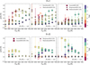 |
Fig. 7 Corrections for Fe I (top) and Fe II (bottom), colour-coded by log g: stars and triangles show 1D NLTE corrections from Bergemann et al. (2012c) and Mashonkina et al. (2011), respectively, and circles show 3D NLTE corrections from Amarsi et al. (2022; available only for dwarf stars). The 1D NLTE corrections for individual stars from Mashonkina et al. (2019a) are shown with crosses (X). The ΔNLTE relation of Ezzeddine et al. (2017) for Fe I is shown with the black line (top row). The squares in the bottom row show the 3D LTE corrections for Fe II from Amarsi et al. (2019). The error bars represent the standard deviation of different lines. |
3.14 Vanadium I
Unfortunately, no detailed NLTE study of vanadium exists in the literature. However, Ou et al. (2020) derived LTE abundances of V I and V II for a large sample of metal-poor stars. From their most reliable measurements they find an ionization imbalance of [V II/V I] = +0.25 and argue that this is most likely due to NLTE effects on the lines of V I. Given that V I is most commonly used to measure vanadium in metal-poor stars, a typical ΔNLTE ≈ +0.25 is expected. We provide [V/Fe]LTE in our fiducial SAGA catalogue, and since the 1D NLTE corrections for V I and Fe I are expected to be of similar order, it is reasonable to expect [V/F]NLTE ≈ [V/Fe]LTE.
3.15 Chromium I
Mean NLTE corrections for 16 optical Cr I lines were calculated from the grid of Bergemann & Cescutti (2010) (see Fig. B.8). The corrections are predominantly positive, with values reaching up to ~1 dex, and tend to increase with increasing temperature and decreasing log g. Overall, the NLTE corrections for the different lines are in good agreement, with σ being much smaller than ΔNLTE in all but a few cases at log g < 1 (see Secion 4.3).
3.16 Manganese I
We computed the average NLTE corrections based on 8 optical Mn I lines from the grid of Bergemann et al. (2019) (see Article number, page 10 of 26 Fig. B.9). Similar to Cr I (see above), the corrections are positive, increasing with increasing temperature and decreasing log g and can reach up to ≳ +1 dex. The corrections are consistent between the different Mn I lines, except at log g < 2.0, where the standard deviation can reach as high as σ > 0.3 (see Sect. 4.3).
Bergemann et al. (2019) computed also 3D NLTE Mn I corrections for selected metal poor models ([Fe/H] = −2 and [Fe/H] = −1). They found that 3D NLTE abundances are typically higher than 1D NLTE abundances by up to 0.15 dex for metal-poor dwarf stars. The difference can be more pronounced for giants, reaching ~0.3 dex for certain Mn lines. However, a full 3D NLTE grid for Mn is currently not available.
3.17 Iron I
In total, 82 Fe I lines were included in the calculated 1D NLTE corrections, using the grids of Mashonkina et al. (2011) and Bergemann et al. (2012c) see Fig. 7 (top). The Fe I corrections are always positive, and increase with decreasing log g and increasing Teff, reaching as high as ~ + 0.5 dex in the most extreme cases. The Mashonkina et al. (2011) and Bergemann et al. (2012c) corrections are in good agreement for all Teff, log g and [Fe/H] values. We adopt their mean values at each stellar parameter set as our fiducial grid.
Amarsi et al. (2022) provides 3D NLTE corrections, but only for FG type dwarfs (Teff = 5000–6500 K, log g = 4–4.5 dex), and metallicities [Fe/H] > −3. Their line list includes only 42 lines that overlap with our fiducial line list, from which we computed the average corrections10. We note that the mean corrections from our fiducial grid (Mashonkina et al. 2011; Bergemann et al. 2012c) differ by less than 0.04 dex when computed for this subset of 42 lines compared to the full line list.
We find that the 3D NLTE corrections of Amarsi et al. (2022) are systematically higher, by up to ~0.2–0.3 dex, compared to the 1D corrections of Bergemann et al. (2012b) and Mashonkina et al. (2011), with the difference increasing with temperature (upper panels of Fig. 7). In addition, the scatter between different Fe I lines is larger in the 3D corrections than in the 1D ones at fixed stellar parameters, yet remains always smaller than 0.12 dex.
For comparison, we also show the 1D NLTE corrections for individual stars from Mashonkina et al. (2019a) in Fig. 7. Those lie approximately 0.1–0.15 dex higher than those of Mashonkina et al. (2011) for the same stellar parameters. In addition, we plot the ΔNLTE-[Fe/H] relation from Ezzeddine et al. (2017), found by fitting 1D NLTE Fe corrections of 22 stars. We note that Ezzeddine et al. (2017) only provide a fit to ΔNLTE as a function of [Fe/H], but not as a function of Teff or log g.
For all three grids, we have adopted corrections for vturb = 1.5 km/s, the peak of the microturbulence distribution of MP stars (Fig. 1). We note that Bergemann et al. (2012b) report that the value of the microturbulence has almost no influence on the size of the NLTE effects. On the other hand, 3D versus 1D corrections are sensitive to the vturb adopted in 1D models. In particular, Amarsi et al. (2022) show that for saturated lines, for vturb = 0 km/s the estimated 3D NLTE versus 1D LTE corrections have similar absolute values as for vturb = 2 km/s but with opposite signs, making the difference between the two as high as 1 dex (see their Fig. 3). The difference between the vturb = 1 km/s and the vturb = 2 km/s is smaller, reaching up to ~0.5 dex at the lowest Teff values.
3.18 Iron II
We provide mean corrections for 12 Fe II optical lines, using the 1D NLTE grid of Bergemann et al. (2012c) and the 3D LTE one of Amarsi et al. (2019); and a subset of 7 lines using the 3D NLTE grid of Amarsi et al. (2022) (see Fig. 7, bottom)10.
The 1D NLTE corrections from Bergemann et al. (2012c) are minimal, ranging from <0.01 to ~0.04 dex. Mashonkina et al. (2019a) report similar values with 1D NLTE corrections for individual stars varying between −0.05 and +0.06 dex (Fig. 7). In contrast, the 3D NLTE corrections from Amarsi et al. (2022) are significantly larger, reaching ~0.2 dex. Notice that the 3D LTE corrections from Amarsi et al. (2019) are often even stronger, with the difference increasing at lower Teff and higher [Fe/H]. This highlights the fact that 3D and NLTE effects often act in opposite directions (e.g. Asplund 2005).
As our fiducial grid, we choose Bergemann et al. (2012c) since it covers the widest parameter range.
3.19 Cobalt I
Using the grid of Bergemann et al. (2010), we computed average NLTE corrections for 17 optical Co I lines (Fig. B.10). The resulting corrections are mainly positive, and increase at higher log g and Teff values, reaching as high as ~+1 dex. The NLTE corrections show significant scatter across the adopted lines, with σ ≳ 0.1 dex for about half the grid points, which is however small compared to the mean corrections (see Sect. 4.3).
3.20 Nickel I
Eitner et al. (2023) computed 1D NLTE Ni abundances for 264 stars from the Gaia-ESO survey and found that the slight sub-solar [Ni/Fe] trend observed at lower [Fe/H] in LTE is reversed under NLTE conditions, where at [Fe/H] ≲ −1 stars exhibit slightly super-solar [Ni/Fe] ratios. The authors provide NLTE corrections only for 12 model atmospheres with Teff = 5750 K and log g = 4.5; Teff = 6500 K and log g = 4.5; and Teff = 5000 K and log g = 3.0, for the metallicities [Fe/H] = −3.0, −2.0, −1.0, 0.0. The corrections are positive and show an increasing trend towards decreasing metallicity, at fixed Teff and log g, reaching 0.2–0.3 dex at [Fe/H] = −3.
Observationally, scatter in [Ni/Fe] is generally low and agrees well between different stellar types (e.g. Cayrel et al. 2004; Roederer et al. 2014). Furthermore, different galaxies agree quite well in their [Ni/Fe] ratios at [Fe/H] < −3 (e.g. Skúladóttir et al. 2024b), arguing against very different NLTE corrections of Ni and Fe. Because of similarities in the structure of the Fe and Ni atoms, it has been argued that likely ΔNLTE(Ni) ≈ ΔNLTE(Fe) (e.g. Skúladóttir et al. 2021). Because of the lack of a more complete grid of NLTE corrections for Ni, we therefore adopt here the conservative approach of providing only [Ni/Fe]LTE, and argue based on the observational evidence that it is reasonable to expect [Ni/Fe]NLTE ≈ [Ni/Fe]LTE. Finally, we note that although the results of Eitner et al. (2023) are not used for our fiducial catalogue, their grid is available for the community through our NLiTE tool, making it very easy to correct a large sample of stars with Ni abundance measurements.
3.21 Copper I
Currently, there is no available NLTE grid for neutral copper. To examine whether we can construct a simple relation between ΔNLTE and different stellar parameters, we compiled available 1D corrections for 37 individual metal poor stars (−4.2 < [Fe/H] < −1) from the studies of Shi et al. (2018), Andrievsky et al. (2018) and Xu et al. (2022).
Figure 2 from Shi et al. (2018), reveals that there is no clear trend between the Cu I corrections and Teff or log g, at least for their sample of 28 stars. There is, however, a clear decreasing trend with metallicity that is also exhibited in the works of Andrievsky et al. (2018) and Xu et al. (2022) (see Fig. 8).
The derived corrections by the three studies are somewhat different; we note that five of the stars shown in Fig. 8 are shared between two or all three of the works. In particular Andrievsky et al. (2018) obtained higher corrections than Shi et al. (2018), while the corrections of Xu et al. (2022) fall in between. These differences likely stem from variations in how inelastic collisions processes with hydrogen are modelled (see discussion in Xu et al. 2022).
Here, we adopt the mean ΔNLTE-[Fe/H] relation based on the three studies, described by the linear least-squares fit to the data:
![Mathematical equation: $\[\Delta \mathrm{NLTE}=-0.26-0.31 \cdot[\mathrm{Fe} / \mathrm{H}]\]$](/articles/aa/full_html/2025/07/aa54228-25/aa54228-25-eq4.png) (4)
(4)
(RMS=0.12), which is shown with a black line in Fig. 8.
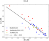 |
Fig. 8 NLTE corrections for Cu I for individual stars by Shi et al. (2018; blue dots), Andrievsky et al. (2018; red dots), and Xu et al. (2022; yellow dots) as a function of [Fe/H]. The black line represents the linear least-squares fit to the data. |
3.22 Zinc I
We computed average 1D NLTE corrections for three Zn I lines, at 4680, 4722 and 4810 Å, which are most commonly used in MP studies (Sitnova et al. 2022). The corrections are given as a function of Teff, log g and [Fe/H], assuming [Zn/Fe] = 0 (Fig. B.11). They are given for [Fe/H] in the range −5 to 0. However, at [Fe/H] < −3.5, Sitnova et al. (2022) provide corrections and measurable EWs only for the UV lines, which are excluded from our study.
At [Fe/H] ≥ −3.5 we find that ΔNLTE for Zn I is primarily positive, 0 dex < ΔNLTE ≲ 0.3 dex, showing an increasing trend with temperature and decreasing log g. Overall the 1D NLTE corrections of the different adopted lines are in very good agreement, with σ ≲ 0.035 dex.
The 1D NLTE corrections for Zn I were also calculated by Takeda et al. (2005) who found typical values of 0 dex ≲ ΔNLTE ≲ 0.1 dex for low-gravity giants, log g < 3, and similar results for higher gravities at [Fe/H] < −1, −0.05 dex ≲ ΔNLTE ≲ 0.1 dex. The ΔNLTE from Takeda et al. (2005) are thus somewhat less strong in comparison to our fiducial grid from Sitnova et al. (2022).
3.23 Strontium II
Mean corrections for the two resonance Sr II lines, at 4077 and 4215 Å, were calculated using the grids of Bergemann et al. (2012a; provided for vturb = 1 km s−1) and Mashonkina et al. (2022) (see Fig. B.12). The two studies are in overall good agreement where they are both defined (within 0.15 dex), and the two lines have very similar corrections. The corrections vary in the range −0.2 ≲ ΔNLTE ≲ +0.4 dex and tend to increase with decreasing [Sr/Fe] and [Fe/H].
We adopt the corrections of Mashonkina et al. (2022) as default, as they span the broadest parameter range.
3.24 Barium II
We calculated average corrections for the five Ba II optical lines (4554, 4934, 5854, 6142, and 6497 Å) that are most commonly used in studies of MP stars, utilizing the grids of Article number, page 12 of 26 Mashonkina & Belyaev (2019) and Gallagher et al. (2020)11 (see B.13). Unlike the common practice, Gallagher et al. (2020) provide their corrections as a function of the 3D NLTE abundance and not the 1DLTE abundance. Therefore, we derived ΔNLTE by interpolating the LTE equivalent widths onto the 1D and 3D NLTE curves of growth. In addition, we computed the mean corrections of Korotin et al. (2015), although these do not include the 4934 Å line and are thus not included in Fig. B.13 (but see Fig. C.7).
The 1D NLTE corrections of Mashonkina & Belyaev (2019) and Gallagher et al. (2020) are in agreement within <0.1 dex. Depending on the stellar parameters, the 3D NLTE corrections of Gallagher et al. (2020) differ from their 1D NLTE corrections by −0.36 to +0.21 dex, typically being higher than the 1D corrections at low Teff, and lower at high Teff. The Korotin et al. (2015) corrections are generally higher (resp. lower) than the Mashonkina & Belyaev (2019) at low (resp. high) Teff, with a maximum difference reaching ~1.5 dex. Similarly to Mashonkina & Belyaev (2019), in all four sets, ΔNLTE tend to decrease with increasing [Ba/Fe].
Andrievsky et al. (2009) computed 1D NLTE corrections for Ba II in 41 VMP stars (−4.19 ≤ [Fe/H] ≤ −2.07) based on the 4554, 5854 and 6497 Å lines. Their corrections range from −0.34 dex to +0.41 dex and are on average ~0.1 dex higher than those of Mashonkina & Belyaev (2019, averaged over the five optical lines) for the same stellar parameters. The difference between the two sets does not show a trend with Teff, log g, [Fe/H] or [Ba II/H].
We choose the Mashonkina & Belyaev (2019) corrections as our fiducial grid, since they span the widest parameter range.
3.25 Europium II
Mean corrections for 6 Eu II optical lines were calculated using the grid of Mashonkina & Gehren (2000) (see Fig. B.14). The corrections are always positive, and tend to increase with decreasing [Fe/H] and [Eu II/Fe], reaching a maximum of ~+0.35 dex. The scatter between the different lines is always small, σ ≲ 0.1.
For comparison, we also plot in Fig. B.14 the mean corrections from the limited grid provided by Mashonkina & Christlieb (2014), which differ by less than 10% (and less than 0.05 dex) from those of Mashonkina & Gehren (2000) for the same stellar parameters.
4 Correcting the SAGA database
4.1 Abundance tables
We apply our NLTE interpolation code, NLiTE, to all metal-poor ([Fe/H] ≤ −1) Milky Way stars in the SAGA database (2023, April 10 version). The results are given in two online tables for all chemical species for the 7367 SAGA entries at [Fe/H] ≤ −1, corresponding to 3296 individual stars. The Kiel diagram of the sample, log g as a function of Teff, is shown in Fig. 9.
Table 2 provides our fiducial NLTE corrected SAGA database obtained by following the approach described in Sect. 2, using the fiducial grids listed in Table A.1. It includes [Fe/H]NLTE, the corrected [X/Fe]NLTE abundance ratios and LTE abundance ratios for N, S, Sc, V and Ni. In case of multiple entries for the same star, in Table 2 we adopt the study which has the highest number of measured elements. The full details of our NLTE corrections for every individual element and SAGA entry (in some cases multiple analyses for the same star) are described in Table 3. Table 4 provides the coordinates and stellar atmospheric parameters of all entries.
The SAGA database is most appropriate for our study as it preferentially compiles 1DLTE abundances. However, occasionally these are not available, and the included abundances are already corrected for NLTE effects, most commonly in the cases of Li, Na, O and Al. When possible, we retrieve the original 1DLTE abundances: for example Cohen et al. (2013) and Bandyopadhyay et al. (2018) apply a constant correction ΔNLTE = +0.6 dex for Al, independent of stellar parameters, based on the results of Baumueller & Gehren (1997). In other cases, it is not straightforward to obtain the 1D LTE abundances, and then they are marked as ‘Originally Corrected’, or (OC) = 1 in the extended Table 3, and we set ΔNLTE=0.
Before applying our corrections, we make sure to exclude all entries with abundances derived through lines that are not included in our line list. In particular, we exclude all abundances derived through infrared or far-UV lines, carbon abundances based on the C2 molecule, oxygen abundances based on the forbidden [OI] line or OH or CO features, iron abundances derived from the Ca II H and K lines, as well as all abundances that involve lines from different ionization states (e.g. Sr abundances derived through Sr I lines, Mn abundances derived through Mn II lines, Ti abundances derived through both Ti I and Ti II lines, e.t.c.). These abundances are omitted from our fiducial NLTE-corrected Table 2 but remain available in the extended Table 3, where they are flagged as ‘Other Wavelength’ (OW) = 1, with ΔNLTE set to NaN.
Extended catalogue including full information on individual NLTE corrections for all SAGA entries.
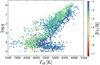 |
Fig. 9 Kiel diagram of all metal-poor SAGA stars, colour-coded by metallicity [Fe/H]. |
4.2 The applied corrections
Here we discuss the results of the NLTE corrections of the SAGA database for selected elements: Fe, Na, Mg, Al, Ti, Cr, and Mn. More details about other elements, as well as the relevant figures can be found in Appendix C.
The 1D NLTE corrections for Fe I applied to all SAGA entries with [Fe/H] ≤ −1 are displayed in Fig. 10. The corrections are based on the average of the Bergemann et al. (2012c) and Mashonkina et al. (2011) grids, which have a maximum discrepancy of 0.16 dex. For stars with parameters outside of the available grid, we select the NLTE correction of the nearest boundary point, as described in Sect. 2.4. The anticorrelation of Δ[Fe/H]1D NLTE with [Fe/H] is clearly visible, and the corrections are in general weakest for the highest log g.
Fig. 11 shows Δ[Na/Fe]1D NLTE and Δ[Al/Fe]1D NLTE as a function of [Fe/H]LTE. These corrections show a more complex trend with [Fe/H] and log g, than seen in Fig. 10. The [Na/Fe] corrections are always negative. At [Fe/H] ≲ −2, where Na abundances are primarily derived from the resonance doublet at 5889/5895, Å, the corrections become stronger with decreasing log g. At higher metallicities the corrections magnitude depends on the lines used, with the weakest corrections (typically >−0.2 dex) observed for stars measured through the subordinate lines at 5682/5688, Å.
For aluminium, no clear trend with log g is observed. At [Fe/H] ≳ −1.5, most Al abundances are based on the subordinate lines, which admit weak corrections. At lower metallicities the corrections are generally stronger, mostly positive and tend to increase with metallicity, driven by the correlation between Δ[Fe/H]1D NLTE and [Fe/H]LTE (Fig. 10). However, several giant stars display negative corrections. This occurs because although Al corrections remain positive in this regime, they are relatively small, whereas the Fe corrections are still significant. Figure 11 therefore shows that it is not always easy to apply a simple relation to estimate the NLTE effects for a given set of stellar parameters.
Figure 12 displays the [Mg/Fe] corrections based on the 1D NLTE grid from Osorio & Barklem (2016; left) and the 3D NLTE grid from Matsuno et al. (2024; right panel). The 1D corrections exhibit a strong dependence on log g and are typically smaller than 0.15 dex. The Mg 3D corrections of Matsuno et al. (2024), available only for FG-type dwarfs, are also positive and exceed those of Osorio & Barklem (2016) by ~0.06 dex on average, with a maximum difference of ~0.14 dex. However, the 3D Fe I corrections of Amarsi et al. (2022) for the same stars exceed their 1D counterparts by a larger margin. As a result, the [Mg I/Fe I] 3D corrections for dwarfs are significantly more negative than their corresponding 1D values. Thus we see that 3D NLTE effects on Fe can have a quite significant impact on the [X/Fe]3D NLTE trend with [Fe/H], even if the element of interest, is not strongly affected by 3D effects.
The Ti ionization imbalance is a decades long problem in the abundance analysis of metal-poor stars. The 1D NLTE corrections for [Ti I/Fe] and [Ti I/Fe] are shown in Fig. 13. We find that the corrections for neutral titanium are strong and positive, ranging from ~+0.1 to +0.5 dex, while those for Ti II are weaker and mostly negative, reaching down to about −0.3 dex. Notably, these differences in the corrections do not align with the observed differences in the measured Ti I and Ti II abundances (Fig. 14). For about 30% of the SAGA MP stars with both abundances available, [Ti I/Ti II] is already positive in LTE. Even in cases where the difference is negative in LTE, the difference in the corrections Δ[Ti I/Ti II]NLTE is significantly higher, meaning that the ionization imbalance would worsen after applying NLTE corrections.
This issue has been previously highlighted by Sitnova et al. (2016), who noted that for more than half of the metal-poor stars they analysed, the agreement between Ti I and Ti II was better in LTE than in NLTE. Similarly, Bergemann (2011) found that the ionization balance for three of the four MP stars they studied worsened in NLTE, and strongly advised against using Ti I abundances in studies of Galactic chemical evolution. More recently, Mallinson et al. (2022) observed that while 1D NLTE corrections improved the ionization balance in some VMP giants, they disrupted it in other metal-poor stars. The authors concluded that consistent 3D NLTE modelling is essential for resolving these discrepancies and advancing the field.
Finally, we show the corrections for [Cr I/Fe] and [Mn I/Fe] in Fig. 15. Both are positive and reaching up to ~+0.8 dex. The [Cr I/Fe] corrections show a pronounced dependence on metallicity, which is also seen to a lesser degree in [Mn I/Fe]. For both Cr and Mn, the corrections increase with decreasing log g at fixed Teff and metallicity (see Figs B.8 and B.9). This trend is reversed here due to the same dependence of the Fe corrections. In addition, the trends for [Mn I/Fe] appear more blurred out due to their strong dependence on effective temperature. These strong 1D NLTE corrections for [Cr/Fe] and [Mn/Fe] result in artificial trends with [Fe/H] in the LTE assumption, which if not corrected can lead to very wrong conclusions about the nucleosynthesis of these elements (see Sect. 5.2.4).
Figs. 10–15 highlight our results when correcting a database with a reality-based distribution of stellar parameters. These results show the diversity in the 1D NLTE corrections for different elements, and their not always straightforward dependence on stellar parameters. Furthermore, we see indications of potentially significant effects when taking the full 3D structure of the stellar atmosphere into account, but unfortunately studies of full 3D NLTE grids are still very limited. With NLiTE we are able to efficiently provide large databases of MP stars with more accurate 1D NLTE abundances using the state-of-the-art grids available.
Coordinates and stellar parameters.
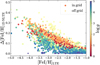 |
Fig. 10 NLTE corrections for Fe I in all metal-poor SAGA stars as a function of their [Fe I/H]LTE, using the mean corrections from Mashonkina et al. (2011) and Bergemann et al. (2012c). The data points are colour-coded by log g. The circles represent stars whose parameters fall within the grid and the star symbols mark those outside the grid boundaries. |
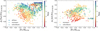 |
Fig. 11 1D NLTE corrections for [Na/Fe] (left) and [Al/Fe] (right) as a function of their [Fe/H]LTE for all MP SAGA stars, derived using the grids from Lind et al. (2022) for Na and Al, and the NLTE Fe I in Fig. 10. Stars with abundances determined from resonance or from subordinate lines are marked with downward and upward triangles, respectively. |
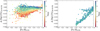 |
Fig. 12 NLTE corrections for [Mg/Fe], colour-coded by log g, for all MP SAGA stars. Left: 1D NLTE corrections from Osorio & Barklem (2016) for Mg I, and Fe I from Fig. 10. Right: 3D NLTE corrections from Matsuno et al. (2024) for Mg I, and Amarsi et al. (2022) for Fe I, defined only for dwarf stars. |
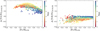 |
Fig. 13 NLTE corrections for [Ti I/Fe] (left) and [Ti II/Fe] (right) for all MP SAGA stars based on Bergemann (2011), and the NLTE Fe I from Fig. 10. |
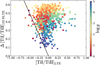 |
Fig. 14 NLTE corrections for [Ti I/Ti II] for all MP SAGA stars, as a function of [Ti I/Ti II]LTE. The black solid line represents Δ[Ti I/Ti II]NLTE = −[Ti I/Ti II]LTE, for which applying the NLTE corrections would result in ionization balance, [Ti I/H]NLTE = [Ti II/H]NLTE. |
4.3 Scatter between lines
A key uncertainty in our approach is how well our average NLTE corrections represent those done line-by-line, i.e. corresponding to the actual (often unknown) line list used for individual stars in the SAGA database. In other words, our average corrections might be shifted in stars where only a portion of our fiducial line list is used, and this might affect global abundance trends. To evaluate the statistical robustness of our corrections, we compute, for each SAGA star and chemical species, the standard deviation of the NLTE corrections across different lines, and provide it in Table 3, along with the number of lines used12. The same information is also available while using the NLiTE tool for individual elements.
Table 5 contains our analysis on the robustness of our method. Let N be the number of detectable lines for a chemical species at given stellar atmosphere and σ ≡ σ(ΔNLTE) the standard deviation of their individual NLTE corrections. If only n lines were used for an observation, the number of possible line combinations (subsets) is:
![Mathematical equation: $\[N_n=\frac{N!}{n!(N-n)!}.\]$](/articles/aa/full_html/2025/07/aa54228-25/aa54228-25-eq5.png) (5)
(5)
The standard deviation of the mean NLTE corrections of all these subsets is:
![Mathematical equation: $\[\sigma_n=\sigma \sqrt{\frac{1}{n}\left(1-\frac{n-1}{N-1}\right)}.\]$](/articles/aa/full_html/2025/07/aa54228-25/aa54228-25-eq6.png) (6)
(6)
If we consider all possible subsets with n = 1, .., N, the overall combined standard deviation is:
![Mathematical equation: $\[\sigma_c=\sqrt{\frac{\sum_{n=1}^N N_n \sigma_n}{\sum_{n=1}^N N_n}}.\]$](/articles/aa/full_html/2025/07/aa54228-25/aa54228-25-eq11.png) (7)
(7)
Furthermore, when N is large, the central limit theorem ensures that the distribution of the mean NLTE corrections from all subsets approaches a normal distribution. An example is shown at the top panel of Fig. 16, where the NLTE corrections of 16 individual Cr I lines, for a star with Teff = 5000 K, log g = 2 and [Fe/H] = −2, are compared to the distribution of the mean corrections of all possible subsets of these lines, which closely follows a Gaussian profile with standard deviation σc.
In such cases, the reliability of our average corrections can be assessed using standard statistical theory. Specifically, in stellar atmospheres where 2σc < |ΔNLTE|/2, there is a >97.7% probability (green shaded area in Fig. 16) that the average correction ΔNLTE improves the abundance estimate, i.e. brings it closer to the true value. Thus, if σc < |ΔNLTE|/4, then applying the correction is preferable to not doing so >97.7% of the time. This analysis does not hold when N is small, as the mean corrections from possible subsets may not approximate a Gaussian. Nevertheless, the threshold σc < |ΔNLTE|/4, still indicates a relatively narrow distribution. We adopt this threshold to assess the reliability of our corrections, and the fraction of stars exceeding this limit for each element is listed in Table 5.
When ΔNLTE is small, σc may surpass this limit despite being negligible in absolute terms. To account for this, we consider all corrections with σc < 0.1 dex to be acceptable, as they lie within the intrinsic uncertainties of NLTE models (see Sect. 4.4) and are unlikely to impact the inferred abundance trends significantly.
Fig. 17 displays σc as a function of ΔNLTE, for all individual SAGA MP stars for Na I and Mn I, which are the worst cases in Table 5. The grey shaded area in each panel represents cases where σc > 0.1 dex and σc > |ΔNLTE|/4, i.e. areas with high scatter, where applying average NLTE corrections could potentially shift LTE abundances away from their true values. For Na I, only 2.5% of stars are in this risky area. As described in Sect. 3.5, for Na I (as for Al I; see Sect. 3.7) separate corrections have been applied to stars observed through resonance and subordinate lines, since these admit very different NLTE corrections. Stars with the largest scatter typically correspond to higher [Fe/H], where both types of lines are detectable and used in abundance calculations (or cases where information on the Na lines are not provided). Instead for Mn I, the largest scatter is seen at low log g ≲ 1.5.
The scatter analysis for the remaining elements shows that the average corrections provide a robust representation of NLTE effects for the vast majority of stars. However, this analysis is not particularly well suited in all cases, e.g. for multiplets with very different ΔNLTE values. In such cases, the abundances are much more likely to be measured from one multiplet (in part due to wavelength coverage of the observed spectra), rather than selecting one line from each multiplet. Different subsets of lines therefore have very different probabilities. This issue has the most significant effects in the case of Na, Al and S, and these elements have therefore been treated specially in this work (Sect. 3.5, 3.7, and 3.9), and for these elements the users of NLiTE are advised to carefully select from the available grids those that correspond best to their line list.
Line-to-line scatter of ΔNLTE in SAGA MP stars.
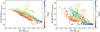 |
Fig. 15 NLTE corrections for [Cr I/Fe] (left) and [Mn I/Fe] (right) for all MP SAGA stars, as a function of [Fe I/H]LTE, using the grids of Bergemann & Cescutti (2010) for Cr I, Bergemann et al. (2019) for Mn I, and the NLTE Fe I from Fig. 10. |
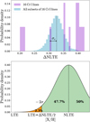 |
Fig. 16 Top: normalized distribution of the NLTE corrections for 16 individual Cr I lines and the mean NLTE corrections of all their possible subsets. Bottom: Illustration of our criterion to assess the reliability of average NLTE corrections. If the line-by-line NLTE value falls within the risky area (orange), applying the average NLTE correction leads to a larger offset compared to adopting the LTE value. The percentages shown correspond to the case where 2σ = |ΔNLTE|/2. |
4.4 Differences between grids
Fig. 18 examines the difference in the NLTE corrections for Fe I, Na I, Mg I and Al I when different grids are applied to MP SAGA stars.
We find that the 1D NLTE corrections for Fe I from Mashonkina et al. (2011) and Bergemann et al. (2012c) are in excellent agreement, differing by less than 0.05 dex for ~95% of the stars. In contrast, the 3D NLTE corrections of Amarsi et al. (2022), available only for dwarf stars with 4 ≤ log g ≤ 4.5, are systematically higher with differences increasing from <0.05 dex at Teff = 5000 K to 0.25–0.3 dex at Teff = 6500 K (see also Sect. 3.17).
The NLTE corrections for Na are also in generally good agreement, with 73% and 92% of stars in the corrections of Lind et al. (2011) and Alexeeva et al. (2014), respectively, differing by less than 0.1 dex from those of our default grid from Lind et al. (2022). The NLTE corrections for Na are predominantly negative across all three grids considered. We note that cases where the corrections differ by more than 0.1 dex between the grids do not show a clear trend with log g, Teff, metallicity or lines used.
For Mg I, our default grid from Osorio & Barklem (2016), is highly consistent with the 1D NLTE grids from Mashonkina (2013), Bergemann et al. (2017), Lind et al. (2022), and Matsuno et al. (2024), with over 95% of stars exhibiting differences of less than 0.1 dex. An exception is the 1D NLTE grid from Merle et al. (2011), which shows stronger positive corrections by ~0.2 dex, on average. The 3D NLTE corrections from Matsuno et al. (2024) are also systematically higher than those from Osorio & Barklem (2016) with the difference being about 0.1 dex at log g = 4 and decreasing with increasing log g.
Bigger discrepancies are observed when considering Al. Here, only 50–60% of stars have corrections that differ less than 0.1 dex between the Nordlander & Lind (2017) 1D and ⟨3D⟩ grids, and our fiducial grid from Lind et al. (2022). At log g ≥ 1.7 the 1D corrections from Nordlander & Lind (2017) are mostly positive and on average 0.08 dex higher than those from Lind et al. (2022). For stars with log g < 1.7, the mean absolute difference between the two grids increases to approximately 0.25 dex. There, the corrections from Nordlander & Lind (2017) are often strong and negative, while those from Lind et al. (2022) remain positive. In this low-log g regime, marked with open circles in Fig. 18, the 1D Nordlander & Lind (2017) corrections appear to have the wrong sign, likely due to issues in the grid or the underlying calculations, and should not be considered reliable (Thomas Nordlander, private communication). The ⟨3D⟩ NLTE corrections of Nordlander & Lind (2017) are always positive and exceed those of Lind et al. (2022) by ~0.15 dex, on average.
The comparison of the corrections derived using different grids for Li I, Si I, K I, Ca I, Ti I, Sr II and Ba II is discussed in Appendix C.
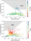 |
Fig. 17 Scatter of mean NLTE corrections from all subsets of lines as a function of ΔNLTE, colour-coded by [Fe/H] (Na) or log g (Mn). The grey areas signify higher uncertainties on the average corrections, i.e. when σc > 0.1 dex and σc > |ΔNLTE|/4. |
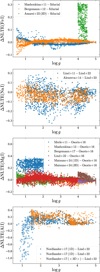 |
Fig. 18 Differences between the NLTE corrections for MP SAGA stars derived using all available grids, from top to bottom, for Fe I, Na I, Mg I and Al I. The fiducial Fe I grid represents the mean corrections from Mashonkina et al. (2011) and Bergemann et al. (2012c). Notice that the range on the y-axes is not always the same. |
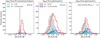 |
Fig. 19 Ionization balance of Fe for all MP SAGA stars for which log g has been derived using the standard spectroscopic method (left), and theoretical isochrones or stellar parallaxes for all MP stars (middle), and only stars with [Fe/H]LTE > −2.5 (right). The shaded histograms are the original LTE distributions of all MP stars (grey) and of dwarf stars (cyan; Teff = [5000, 6500], log g = [4, 4.5]). Red and blue show the corresponding distributions after applying 1D NLTE corrections for all stars (Bergemann et al. 2012c) and 3D NLTE corrections for the dwarf sample (Amarsi et al. 2022), respectively. |
4.5 The Fe I-Fe II ionization balance
Stellar parameters are most commonly determined based on either the spectroscopic or the photometric method. In simplified terms, the spectroscopic method adjusts the stellar parameters so that all Fe I and Fe II lines give consistent Fe measurements. However, this is often done in LTE, neglecting NLTE effects that can strongly affect iron lines in a different way, e.g. Fe I vs. Fe II lines, especially at low metallicity (see e.g. Mucciarelli & Bonifacio 2020). This can result in unreliable results, e.g. in surface gravities being underestimated by up to ~0.5 dex, which results in lower [Fe/H] abundances (e.g. Sitnova et al. 2015). Alternatively, the stellar parameters can be based on photometry and distance estimates to the star, e.g. with parallaxes and isochrone fitting and/or other empirical relations (Flower 1996; Sitnova et al. 2015; Mashonkina et al. 2017a; Mucciarelli & Bonifacio 2020). These methods should be less sensitive to possible NLTE effects.
Fig. 19 shows the distribution of the ionization balance, [Fe I/Fe II], for the SAGA database. We include only stars with parameters that lie within the respective grid limits (see Table A.1). For stars with surface gravities computed through the standard spectroscopic method (1077 entries), the original LTE [Fe I/H] and [Fe II/H] abundances were forced to agree with each other. Therefore, as expected, after applying the NLTE corrections the ionization balance becomes worse: the scatter increases and the peak moves at +0.1 dex in 1D NLTE and at +0.22 dex in 3D NLTE (available for 97 stars). This is a direct consequence of the fact that the NLTE corrections are systematically higher for Fe I than for Fe II (see Fig. 7).
On the other hand, when log g is determined from photometry (1332 entries; middle panel of Fig. 19), in LTE the [Fe I/H] is on average lower than [Fe II/H] by ~0.065 dex. In this case, we would expect NLTE corrections to bring the distribution closer to equilibrium. Indeed, in 1D NLTE, the ionization balance shows modest improvement, with the mean offset reducing to +0.047 dex. The 3D NLTE corrections (available for 199 stars), instead, appear to worsen the agreement, shifting the peak to +0.13 dex and increasing the scatter from 0.14 to 0.16 dex.
These findings align with previous studies suggesting that current models may overestimate NLTE departures for Fe I at low [Fe/H]. For example, Mashonkina et al. (2019a) report that at [Fe/H] < −3.5, 1D NLTE Fe I abundances exceed Fe II abundances by up to +0.35 dex in five out of six cases. Similarly, in Bergemann et al. (2012c) the ionization balance of their only EMP star analysed worsens in NLTE compared to LTE (though they note that the parallax of this star is highly uncertain), and Amarsi et al. (2022) find poor ionization balance for one of their two analysed VMP stars.
Indeed, if we consider only stars with [Fe/H] > −2.5 (right panel of Fig. 19) the situation improves. In 1D NLTE, 61% of stars have −0.1 < [Fe I/Fe II] < +0.1 compared to 52% in LTE, and the peak shifts from −0.05 to 0.0 dex, while in 3D NLTE, the average offset decreases now to +0.09 dex. For science cases that require high precision and accuracy, improvement of both the NLTE models and the chemical abundance analysis is advised.
4.6 Impact on the SAGA MDF
Fig. 20 illustrates the impact on the SAGA metallicity distribution function (MDF) after applying the mean 1D-NLTE Fe I corrections from Mashonkina et al. (2011) and Bergemann et al. (2012c). Here, we include only individual stars; in cases where multiple entries from different surveys/authors exist for the same star, we keep the one with the highest number of measured abundances, as in Table 2. We find that the SAGA MDF becomes steeper and its peak shifts from [Fe/H] = −2.7 to [Fe/H] = −2.5. The number of EMP stars ([Fe/H] ≤ −3) decreases by 31%, i.e. from 526 in LTE to 363 in NLTE; we note that here only stars with Fe I and/or Fe II measurements are included. We therefore recommend that careful studies of metal-poor MDFs take NLTE effects into account, which can be done easily with NLiTE for large databases.
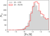 |
Fig. 20 Metallicity distribution function of all MP SAGA stars in LTE (grey) and after applying our fiducial 1D NLTE corrections (red). |
5 Comparison with the NEFERTITI model
The main goal of this work is to provide a large fully NLTE-corrected database of MP stars that can be contrasted against chemical evolution models in a meaningful way. In an upcoming publication (Koutsouridou et al. in prep.) we will go into detail on how combining these data with our models can help constrain the properties of the first stars and early chemical enrichment. Here instead, we focus more on the technical aspect of how adding the NLTE corrections affects the comparison with the predictions of our cosmological galaxy formation and chemical enrichment model NEFERTITI (NEar FiEld cosmology: ReTracing Invisible TImes), described in detail in Koutsouridou et al. (2023).
5.1 Description of the NEFERTITI model
NEFERTITI is a state-of-the-art semi-analytical model that runs on halo merger trees derived from N-body cosmological simulations or Monte Carlo techniques. It builds upon previous semi-analytical models for the Local Group formation (Salvadori et al. 2007; Salvadori et al. 2010, 2015; Pagnini et al. 2023).
The model follows the flow of baryons from the intergalactic medium (IGM) into the dark matter (DM) halos, the formation of stars and stellar evolution within each galaxy, and the return of mass and metals into the interstellar medium (ISM) and the IGM through stellar feedback. In addition, it traces the position and dynamics of baryons (gas and stars) through their associated DM particles and is therefore able to probe the spatial distribution of all stellar populations down to redshift z = 0. Stars form in DM halos that surpass a minimum mass, which evolves through cosmic times to account for the effects of photodissociating and ionizing radiation (Salvadori & Ferrara 2009). The IGM initially has a primordial composition enabling the formation of Pop III stars in the first star-forming halos. Once the metallicity within a halo exceeds the critical value Zcrit = 5.15 × 10⁻⁵ Z⊙ (Caffau et al. 2011; de Bennassuti et al. 2017), assuming Z⊙ = 0.0134 (Asplund et al. 2009), normal (Pop II/I) stars form according to a Larson Initial Mass Function (IMF) with m⋆ = [10 − − 100] M⊙ and a peak at mch = 0.35 M⊙. The IMF of both Pop III and Pop II/I stars is stochastically sampled (as in Rossi et al. 2021) and the evolution of individual stars is followed in their proper timescales.
In this study, we employ NEFERTITI coupled with a cold dark matter (DM) N-body simulation of a Milky Way analogue (fully described in Koutsouridou et al. 2023), which successfully reproduces the present-day global properties of the Milky Way (metallicity and mass of both stars and gas) and the metallicity distribution function of the Galactic halo (Bonifacio et al. 2021). We adopt the yields of Heger & Woosley (2002, 2010) for Pop III stars and those of Karakas (2010) and Limongi & Chieffi (2018) for Pop II/I stars. Here, we assume a Larson IMF for Pop III stars, with m⋆ = [0.8, 1000] M⊙ and mch = 10 M⊙, consistent with stellar archaeology observations (Rossi et al. 2021; Pagnini et al. 2023; Koutsouridou et al. 2024). We note that varying the Pop III IMF or the energy distribution of Pop III supernovae (SNe) can impact the overall extent of the predicted [X/Fe]–[Fe/H] distributions and influence the number of surviving stars in each bin. However, these variations have a minimal effect on the bulk of present-day metal-poor (MP) stars, which are dominated by normal Pop II enrichment (Koutsouridou et al. 2023), represented by the dark grey regions in Figs. 21–24.
5.2 Comparison to the NLTE-SAGA database
In the following subsections, we compare the NLTE-SAGA database with our NEFERTITI model. Figures 21–24 display the comparison for selected elements, both in LTE and NLTE. We include predictions for the chemical abundances of both the descendants of Pop III stars (light grey, low-density regions) and those of Pop I and II stars (dark grey, high-density regions), which represent the bulk of the stellar population (Koutsouridou et al. 2023). In all of the following discussion our fiducial Fe I abundance corrections are adopted (see Fig. 10). Discussion on additional elements can be found in Appendix D.
5.2.1 Carbon predictions
The elemental abundance that is perhaps the most indicative of pollution from Pop III stars is carbon. Figure 21 displays the [C/Fe]-[Fe/H] distribution of all individual stars with CH measurements (left) and after applying the CH 3D NLTE corrections of Norris & Yong (2019) and the average Fe I NLTE corrections from Mashonkina et al. (2011) and Bergemann et al. (2012c) (middle panel). In the right panel we have additionally applied the evolutionary corrections for carbon from Placco et al. (2014)13. The grey shaded areas, identical across all panels, depict the distribution of all stars surviving in the Galactic halo at z = 0 as predicted by our model. The stars residing in the light grey area have received ≥ 50% of their metals from Pop III stars, while the dark grey regions correspond to stars whose metals come mainly (>50%) from Pop I/II stars.
In Koutsouridou et al. (2023), we showed that our model failed to reproduce the UMP ([Fe/H] ≤ −4) stars with the highest A(C) ≳ 6–6.5, a problem faced by several other studies (e.g. Cooke & Madau 2014; Magg et al. 2020; Komiya et al. 2020; Chiaki et al. 2020; Jeon et al. 2021; Rizzuti et al. 2025). In this region, the enrichment of CEMP stars is predicted to be dominated by Pop III SNe (e.g. Koutsouridou et al. 2023). Komiya et al. (2020) showed that even assuming an extremely inefficient mixing of SN yields does only partially reproduce these stars while introducing inconsistencies in the metallicity distribution function. Rossi et al. (2023), using a model calibrated on the UFD Böotes I, proposed that these stars might form through enrichment by Pop II asymptotic giant branch (AGB) stellar winds after a powerful SN expels all gas from a halo, along with the iron-rich signature of Pop II SNe. Here, we find that accounting for NLTE effects resolves this discrepancy: all UMP stars now align with the predictions of our model, even after correcting for evolutionary effects (middle and right panels of Fig. 21).
At [Fe/H] > −4, there are still several stars that lie above our predicted distribution. Most of them are CEMP-s stars, i.e. stars enriched in s-process elements ([Ba/Fe] ≥ 0, marked with circles in Fig. 21) that are believed to have acquired their carbon by mass transfer from an AGB companion (e.g. Aoki et al. 2007; Starkenburg et al. 2014; Hansen et al. 2016). Since our model does not currently account for binary systems, it is expected that CEMP-s stars are not reproduced.
However, a small number of CEMP-no stars (X symbols), whose abundances are thought to reflect their birth environment, also fall above our predictions at [Fe/H] > −4. Additionally, NLTE corrections shift some stars to lower carbon abundances, causing them to drop below our distribution. However, the bulk of the [C/Fe] measurements do fall within our predictions, giving a generally good agreement (right panel).
As seen in the left panel of Fig. 21, the SAGA stars exhibit an increasing [C/Fe] with log g at fixed metallicity, a pattern that persists in NLTE (middle panel), since the empirical corrections of Norris & Yong (2019) are independent of log g. Although this trend weakens after applying the Placco corrections, it does not fully disappear. Therefore, it is possible that once more physically motivated corrections for CH become available, the scatter at fixed [Fe/H] could further decrease, improving even more the alignment with our theoretical predictions.
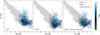 |
Fig. 21 Metal-poor Galactic halo stars in the [C/Fe]–[Fe/H] diagram as predicted by our NEFERTITI model: Pop III descendants (in light grey) and Pop I/II descendants (in dark grey). The data points show all SAGA MP stars colour-coded by log g: in LTE (left); in NLTE (middle); and after applying both the NLTE and the C evolutionary corrections (right). Crosses (X) show CEMP-no stars ([Ba/Fe] < 0), circles show CEMP-s stars ([Ba/Fe] > 0) and triangles stars with unknown Ba. |
5.2.2 Light elements Na and Al
The [Na/Fe]–[Fe/H] distribution of SAGA stars in LTE shows significant scatter, particularly in the range −4 ≤ [Fe/H] ≤ −2, where many stars exceed our model predictions by up to ~3 dex (Fig. 22; top). Such high [Na/Fe] ratios are produced only by Pop III SNe; however, their iron yields are too small by two-three orders of magnitude to account for these observations. Correcting for NLTE effects (Lind et al. 2022) improves significantly the agreement with our predictions. The peak of the [Na/Fe] distribution shifts from [Na/Fe] = −0.05 to [Na/Fe] = −0.25, and the scatter is notably reduced14 from σ = 0.47 to σ = 0.37. As a result, the number of stars lying above our predicted distribution decreases by 75%. In addition, most of these stars are outside the limits of our adopted NLTE grid (marked as circles), [Na/Fe]LTE > +0.8. Therefore, it is possible that even stronger negative corrections may apply to these stars, which could bring them into closer agreement with our model.
The NLTE corrections for [Al/Fe] are also strong, drastically shifting the peak of the observed distribution from [Al/Fe] = −0.75 to [Al/Fe] = −0.35 as shown in the rightmost bottom panel of Fig. 22. Although the scatter decreases only slightly, the predominantly positive corrections improve the agreement with the model predictions. Fewer stars now fall below the model distribution, though some move above it under NLTE. We note that when adopting the 1D NLTE corrections from Nordlander & Lind (2017), instead of the Lind et al. (2022) ones, the scatter increases significantly, from σ = 0.37 to σ = 0.51 with several stars in the range −4 ≤ [Fe/H] ≤ −2 and log g < 1.5, acquiring strong negative corrections, and falling below our predicted distribution, to values as low as [Al/Fe] ≃ −2 (see Sect. 4.4). In contrast, when using the ⟨3D⟩ corrections from Nordlander & Lind (2017) the [Al/Fe] corrections are always positive, thus, in this case no stars occupy the region at [Al/Fe] < −1, and the scatter reduces to σ = 0.35.
5.2.3 Alpha-elements Mg and Ca
Fig. 23 displays the SAGA [Mg/Fe]–[Fe/H] (top) and [Ca/Fe]–[Fe/H] (bottom) distributions in comparison to our model predictions. NLTE corrections have a minimal impact on the observed distributions. For [Mg/Fe], they slightly reduce the scatter from 0.21 to 0.20, while for [Ca/Fe], the distribution remains virtually unchanged. In both cases, the observed distributions align well with our theoretical ones, with a few outliers.
5.2.4 Iron-peak elements Cr and Mn
Fig. 24, displays the distribution of SAGA stars in the [Cr/Fe]–[Fe/H] (top) and [Mn/Fe]–[Fe/H] (bottom) diagrams, using the 1D NLTE grids of Bergemann & Cescutti (2010) for Cr and Bergemann et al. (2019) for Mn.
In LTE, both of these distributions show a downward trend with decreasing [Fe/H] which disappears after applying the NLTE corrections. The NLTE [Mn/Fe]–[Fe/H] mean relation becomes flat while the [Cr/Fe]–[Fe/H] shows a slightly upward trend, with [Cr/Fe] increasing with decreasing [Fe/H]. The peaks of both distributions significantly shift upwards: from −0.15 to +0.15 for [Cr/Fe] and from −0.45 to −0.15 for [Mn/Fe]. NLTE corrections do not reduce the scatter in these cases.
Applying NLTE corrections reduces the number of stars with [Cr/Fe] ≤ −0.4, which are not reproduced by our model. However, the corrected [Cr/Fe] distribution now tends to lie on the high side of model predictions, similar to other Fe-peak elements such as Co and Zn (see Fig. D.4 in Appendix D). Noticeably, the discrepancy pertains the bulk of the stellar population, and thus it is likely linked to the production mechanism of Fe-peak elements from Pop II/I stars, or possibly to inaccuracies in the NLTE corrections or lack of consideration for 3D effects. Since the corrections for these elements can be large, up to |ΔNLTE| ≈ 1 (see Figs. B.8 and B.9), some uncertainty is expected. Although beyond the scope of this paper, it is interesting to note that a contribution of Pop II hypernovae with [Fe/H] ≈ −1 might partially alleviate the problem, producing super-solar values of [Cr, Zn/Fe] (and [Al/Fe]) while leaving [Mn/Fe] unaltered (e.g. see Fig. 9 from the review of Nomoto et al. 2013). Both in the case of Cr and Mn, the abundance trend is significantly altered when applying NLTE corrections. We therefore emphasize that it is misleading to discuss chemical evolution and nucleosynthesis of these elements without fully taking NLTE effects into account.
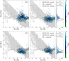 |
Fig. 22 Distribution of MP Galactic halo stars in the [Na/Fe]–[Fe/H] (top) and [Al/Fe]–[Fe/H] (bottom) diagrams, as predicted by the NEFERTITI model: Pop III descendants (in light grey) and Pop I/II descendants (in dark grey). The data points represent all MP SAGA stars, colour-coded with log g, in LTE (left) and NLTE (right). Stars with parameters within the grids are marked with crosses (X), while circles indicate stars outside these limits. Triangles represent stars whose published abundances were already corrected for NLTE effects. The right marginal plots compare the SAGA [Na/Fe] and [Al/Fe] distributions in LTE (blue) and NLTE (black), excluding stars with upper or lower limits. The standard deviations of the distributions are noted at the top. |
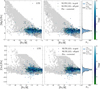 |
Fig. 23 Same as Fig. 22, but for [Mg/Fe] (top) and [Ca/Fe] (bottom); observed abundances have been corrected using the grids of Osorio & Barklem (2016) for Mg, Mashonkina et al. (2017b) for Ca I and the mean corrections of Mashonkina et al. (2011) and Bergemann et al. (2012c) for Fe I. |
6 Summary and conclusions
Metal-poor ([Fe/H] ≤ −1) stars provide a unique window into the early Universe, but accurately interpreting their chemical abundances requires accounting for non-LTE (NLTE) effects, which are often neglected in large stellar samples. For the first time, we have provided a fully NLTE-corrected catalogue of all MP stars in the SAGA database, reaching down to the lowest metallicities, [Fe/H] < −4. In addition, we have developed NLiTE15, an online tool designed for the community to efficiently apply NLTE corrections to large stellar samples of MP stars. To complete this task we have undergone a detailed review of the currently available state-of-the-art 1D and 3D NLTE grids in the literature (Sect. 3). Together with the NLiTE tool, this allowed us to do an extensive comparison of the available grids in order to understand uncertainties of the NLTE calculations for individual elements.
The NLiTE tool (Sect. 2) provides corrections for 24 chemical species from Li to Eu, by interpolating within precomputed NLTE grids, which depend on the stellar atmospheric parameters: Teff, log g, [Fe/H], and, when relevant, A(X) or [X/Fe]. These grids are based on publicly available NLTE datasets (Table A.1) that are originally linked to specific spectral lines. However, in the SAGA database the original selection of lines is not always available. The novelty of NLiTE is that it is averaged over a predetermined line list (Table 1). The selected lines are those most frequently used to measure chemical abundances in MP stars, using optical spectra (3 500 Å ≲ λ ≲ 10 000 Å). Our selection takes into account line detectability for each set of stellar parameters (see Sect. 2.1). We find that in most cases the scatter between the ΔNLTE corrections of different line sets is small σlines < 0.1 dex, and/or small in comparison to the mean correction (Sect. 4.3).
A full NLTE-SAGA catalogue is provided for MP stars in the Milky Way, obtained using NLiTE (Tables 2 and 3). We find that the magnitudes and signs of NLTE corrections vary significantly depending on the chemical species and do not always show a straightforward dependence on stellar parameters (Sect. 4.2). The strongest [Element/Fe] NLTE corrections reaching >0.5 dex are found for Na, Al, Si, K, Cr, Mn, and Co. Significant corrections are found for Fe I, spanning from 0 to +0.4 dex, that shift the SAGA metallicity distribution to higher [Fe/H] (Sect. 4.6), decreasing the number of [Fe/H] ≤ −3 stars by 31%. Therefore we strongly encourage including NLTE effects when studying the metallicity distribution of the Galactic halo.
A detailed comparison between different 1D NLTE grids (Sect. 3) reveals a generally good agreement for Li, Fe, Mg, K, Ca, Ti II, Sr and Ba with corrections for over 90% of stars differing by less than 0.1 dex and maximum discrepancies of <0.2 dex (Sect. 4.2). Larger discrepancies are found for Na and O I (up to 0.30 dex), Al (up to 0.55 dex), and Si I (up to 0.87 dex). In general, quite significant discrepancies can be found when comparing 1D and 3D NLTE corrections, e.g. in the case of O, Mg, Al, Fe and Ba (Sect. 3). This highlights that full 3D NLTE corrections are needed for highly accurate abundances. Unfortunately, there is still a lack of 3D NLTE grids that cover the full range of typical stellar parameters.
We compared the NLTE-SAGA catalogue to predictions from NEFERTITI, our cosmological model for galaxy formation and evolution (Koutsouridou et al. 2023). Incorporating 3D NLTE effects resolves a key discrepancy for stars with [Fe/H] < −3.5, which previously exhibited higher [C/Fe] than predicted by models (e.g. de Bennassuti et al. 2017; Komiya et al. 2020; Rossi et al. 2023; Koutsouridou et al. 2023). After applying NLTE corrections, the observed carbon abundances align well with our theoretical predictions (Sect. 5). NLTE corrections also significantly improve the agreement between observed and theoretical Na abundances, reducing the number of stars with higher-than-expected [Na/Fe] by 75%. Similarly, positive Al corrections bring the observed distribution closer to theoretical predictions.
The levels of Mg and Ca relative to Fe remain largely consistent with model predictions and exhibit minimal sensitivity to NLTE effects. For Si, Cr, and Mn, previously observed metallicity trends diminish, and their distributions are broadly in line with theoretical expectations. In contrast, K, Ti, Co, and Zn remain underproduced in the model compared to observations, a common issue in galactic chemical evolution studies (e.g. Romano et al. 2010; Zhao et al. 2016; Kobayashi et al. 2020; Rossi et al. 2024b). NLTE corrections mitigate but do not fully resolve this discrepancy for K, while they exacerbate it for Ti I, Co, and Zn. Meanwhile, Cu remains within the predicted distribution both before and after applying NLTE corrections.
This study demonstrates the crucial role of NLTE corrections in refining stellar abundance measurements, improving consistency with chemical evolution models, and offering new insights into the nucleosynthetic history of the Milky Way. By providing more accurate abundance measurements, NLiTE ensures that theoretical predictions can be tested against reliable data, preventing erroneous conclusions and enhancing our understanding of the first stars and early chemical evolution.
Data availability
Full Tables 1, 2, 3 and 4 are available at the CDS via anonymous ftp to cdsarc.cds.unistra.fr (130.79.128.5) or via https://cdsarc.cds.unistra.fr/viz-bin/cat/J/A+A/699/A32 The tables are also provided in .tsv format at https://nlite.pythonanywhere.com/.
Appendices A–D are available at https://zenodo.org/records/15468109.
Acknowledgements
This project has received funding from the European Research Council Executive Agency (ERCEA) under the European Union’s Horizon Europe research and innovation program (acronym TREASURES, grant agreement No 101117455”). I.K. and S.S. acknowledge ERC support (grant agreement No. 804240). We thank the following experts for insightful discussion and suggestions that helped improve the paper: A.M. Amarsi, M. Bergemann, K. Lind, L. Mashonkina, and T. Nordlander.
References
- Alexeeva, S. A., & Mashonkina, L. I. 2015, MNRAS, 453, 1619 [NASA ADS] [CrossRef] [Google Scholar]
- Alexeeva, S. A., Pakhomov, Y. V., & Mashonkina, L. I. 2014, Astron. Lett., 40, 406 [NASA ADS] [CrossRef] [Google Scholar]
- Amarsi, A. M., & Asplund, M. 2017, MNRAS, 464, 264 [Google Scholar]
- Amarsi, A. M., Nissen, P. E., & Skúladóttir, Á. 2019, A&A, 630, A104 [NASA ADS] [CrossRef] [EDP Sciences] [Google Scholar]
- Amarsi, A. M., Lind, K., Osorio, Y., et al. 2020, A&A, 642, A62 [EDP Sciences] [Google Scholar]
- Amarsi, A. M., Liljegren, S., & Nissen, P. E. 2022, A&A, 668, A68 [NASA ADS] [CrossRef] [EDP Sciences] [Google Scholar]
- Andrievsky, S. M., Spite, M., Korotin, S. A., et al. 2007, A&A, 464, 1081 [NASA ADS] [CrossRef] [EDP Sciences] [Google Scholar]
- Andrievsky, S. M., Spite, M., Korotin, S. A., et al. 2008, A&A, 481, 481 [NASA ADS] [CrossRef] [EDP Sciences] [Google Scholar]
- Andrievsky, S. M., Spite, M., Korotin, S. A., et al. 2009, A&A, 494, 1083 [NASA ADS] [CrossRef] [EDP Sciences] [Google Scholar]
- Andrievsky, S. M., Spite, M., Korotin, S. A., et al. 2010, A&A, 509, A88 [NASA ADS] [CrossRef] [EDP Sciences] [Google Scholar]
- Andrievsky, S., Bonifacio, P., Caffau, E., et al. 2018, MNRAS, 473, 3377 [NASA ADS] [CrossRef] [Google Scholar]
- Aoki, W., Beers, T. C., Christlieb, N., et al. 2007, ApJ, 655, 492 [NASA ADS] [CrossRef] [Google Scholar]
- Asplund, M. 2005, ARA&A, 43, 481 [Google Scholar]
- Asplund, M., Carlsson, M., & Botnen, A. V. 2003, A&A, 399, L31 [NASA ADS] [CrossRef] [EDP Sciences] [Google Scholar]
- Asplund, M., Grevesse, N., Sauval, A. J., & Scott, P. 2009, ARA&A, 47, 481 [NASA ADS] [CrossRef] [Google Scholar]
- Bandyopadhyay, A., Sivarani, T., Susmitha, A., et al. 2018, ApJ, 859, 114 [Google Scholar]
- Barklem, P. S., Belyaev, A. K., & Asplund, M. 2003, A&A, 409, L1 [NASA ADS] [CrossRef] [EDP Sciences] [Google Scholar]
- Barklem, P. S., Christlieb, N., Beers, T. C., et al. 2005, A&A, 439, 129 [NASA ADS] [CrossRef] [EDP Sciences] [Google Scholar]
- Baumueller, D., & Gehren, T. 1997, A&A, 325, 1088 [NASA ADS] [Google Scholar]
- Beers, T. C., & Christlieb, N. 2005, ARA&A, 43, 531 [NASA ADS] [CrossRef] [Google Scholar]
- Bergemann, M. 2011, MNRAS, 413, 2184 [NASA ADS] [CrossRef] [Google Scholar]
- Bergemann, M., & Cescutti, G. 2010, A&A, 522, A9 [NASA ADS] [CrossRef] [EDP Sciences] [Google Scholar]
- Bergemann, M., Pickering, J. C., & Gehren, T. 2010, MNRAS, 401, 1334 [CrossRef] [Google Scholar]
- Bergemann, M., Hansen, C. J., Bautista, M., & Ruchti, G. 2012a, A&A, 546, A90 [NASA ADS] [CrossRef] [EDP Sciences] [Google Scholar]
- Bergemann, M., Kudritzki, R.-P., Plez, B., et al. 2012b, ApJ, 751, 156 [Google Scholar]
- Bergemann, M., Lind, K., Collet, R., Magic, Z., & Asplund, M. 2012c, MNRAS, 427, 27 [Google Scholar]
- Bergemann, M., Kudritzki, R.-P., Würl, M., et al. 2013, ApJ, 764, 115 [NASA ADS] [CrossRef] [Google Scholar]
- Bergemann, M., Collet, R., Amarsi, A. M., et al. 2017, ApJ, 847, 15 [NASA ADS] [CrossRef] [Google Scholar]
- Bergemann, M., Gallagher, A. J., Eitner, P., et al. 2019, A&A, 631, A80 [NASA ADS] [CrossRef] [EDP Sciences] [Google Scholar]
- Bergemann, M., Hoppe, R., Semenova, E., et al. 2021, MNRAS, 508, 2236 [NASA ADS] [CrossRef] [Google Scholar]
- Bonifacio, P., Monaco, L., Salvadori, S., et al. 2021, A&A, 651, A79 [NASA ADS] [CrossRef] [EDP Sciences] [Google Scholar]
- Brauer, K., Mead, J., Wise, J. H., et al. 2025, ApJ, submitted, [arXiv:2502.20433] [Google Scholar]
- Caffau, E., Bonifacio, P., François, P., et al. 2011, Nature, 477, 67 [NASA ADS] [CrossRef] [Google Scholar]
- Cayrel, R., Depagne, E., Spite, M., et al. 2004, A&A, 416, 1117 [NASA ADS] [CrossRef] [EDP Sciences] [Google Scholar]
- Chiaki, G., Wise, J. H., Marassi, S., et al. 2020, MNRAS, 497, 3149 [NASA ADS] [CrossRef] [Google Scholar]
- Cohen, J. G., Christlieb, N., Thompson, I., et al. 2013, ApJ, 778, 56 [Google Scholar]
- Collet, R., Asplund, M., & Trampedach, R. 2006, ApJ, 644, L121 [NASA ADS] [CrossRef] [Google Scholar]
- Collet, R., Asplund, M., & Trampedach, R. 2007, A&A, 469, 687 [NASA ADS] [CrossRef] [EDP Sciences] [Google Scholar]
- Collet, R., Nordlund, Å., Asplund, M., Hayek, W., & Trampedach, R. 2018, MNRAS, 475, 3369 [NASA ADS] [CrossRef] [Google Scholar]
- Cooke, R. J., & Madau, P. 2014, ApJ, 791, 116 [Google Scholar]
- Cooke, R., Pettini, M., Steidel, C. C., Rudie, G. C., & Nissen, P. E. 2011, MNRAS, 417, 1534 [CrossRef] [Google Scholar]
- de Bennassuti, M., Salvadori, S., Schneider, R., Valiante, R., & Omukai, K. 2017, MNRAS, 465, 926 [NASA ADS] [CrossRef] [Google Scholar]
- de Jong, R. S., Agertz, O., Berbel, A. A., et al. 2019, The Messenger, 175, 3 [NASA ADS] [Google Scholar]
- Dobrovolskas, V., Kučinskas, A., Steffen, M., et al. 2013, A&A, 559, A102 [NASA ADS] [CrossRef] [EDP Sciences] [Google Scholar]
- Eitner, P., Bergemann, M., Ruiter, A. J., et al. 2023, A&A, 677, A151 [NASA ADS] [CrossRef] [EDP Sciences] [Google Scholar]
- Ezzeddine, R., Frebel, A., & Plez, B. 2017, ApJ, 847, 142 [Google Scholar]
- Fabbian, D., Asplund, M., Carlsson, M., & Kiselman, D. 2006, A&A, 458, 899 [CrossRef] [EDP Sciences] [Google Scholar]
- Fabbian, D., Asplund, M., Barklem, P. S., Carlsson, M., & Kiselman, D. 2009a, A&A, 500, 1221 [NASA ADS] [CrossRef] [EDP Sciences] [Google Scholar]
- Fabbian, D., Nissen, P. E., Asplund, M., Pettini, M., & Akerman, C. 2009b, A&A, 500, 1143 [NASA ADS] [CrossRef] [EDP Sciences] [Google Scholar]
- Fields, B. D. 2011, Annu. Rev. Nucl. Part. Sci., 61, 47 [CrossRef] [Google Scholar]
- Flower, P. J. 1996, ApJ, 469, 355 [NASA ADS] [CrossRef] [Google Scholar]
- Frebel, A., Collet, R., Eriksson, K., Christlieb, N., & Aoki, W. 2008, ApJ, 684, 588 [NASA ADS] [CrossRef] [Google Scholar]
- Fulbright, J. P. 2000, AJ, 120, 1841 [NASA ADS] [CrossRef] [Google Scholar]
- Gaia Collaboration (Babusiaux, C., et al.) 2018a, A&A, 616, A10 [NASA ADS] [CrossRef] [EDP Sciences] [Google Scholar]
- Gaia Collaboration (Helmi, A., et al.) 2018b, A&A, 616, A12 [NASA ADS] [CrossRef] [EDP Sciences] [Google Scholar]
- Gallagher, A. J., Caffau, E., Bonifacio, P., et al. 2016, A&A, 593, A48 [NASA ADS] [CrossRef] [EDP Sciences] [Google Scholar]
- Gallagher, A. J., Bergemann, M., Collet, R., et al. 2020, A&A, 634, A55 [NASA ADS] [CrossRef] [EDP Sciences] [Google Scholar]
- Hansen, T. T., Andersen, J., Nordström, B., et al. 2016, A&A, 588, A3 [NASA ADS] [CrossRef] [EDP Sciences] [Google Scholar]
- Hartwig, T., Bromm, V., Klessen, R. S., & Glover, S. C. 2015, MNRAS, 447, 3892 [NASA ADS] [CrossRef] [Google Scholar]
- Hartwig, T., Yoshida, N., Magg, M., et al. 2018, MNRAS, 478, 1795 [CrossRef] [Google Scholar]
- Hartwig, T., Ishigaki, M. N., Klessen, R. S., & Yoshida, N. 2019, MNRAS, 482, 1204 [NASA ADS] [CrossRef] [Google Scholar]
- Heger, A., & Woosley, S. E. 2002, ApJ, 567, 532 [Google Scholar]
- Heger, A., & Woosley, S. E. 2010, ApJ, 724, 341 [Google Scholar]
- Ishigaki, M. N., Chiba, M., & Aoki, W. 2012, ApJ, 753, 64 [NASA ADS] [CrossRef] [Google Scholar]
- Ishigaki, M. N., Tominaga, N., Kobayashi, C., & Nomoto, K. 2018, ApJ, 857, 46 [Google Scholar]
- Jacobson, H. R., Keller, S., Frebel, A., et al. 2015, ApJ, 807, 171 [NASA ADS] [CrossRef] [Google Scholar]
- Jeon, M., Bromm, V., Besla, G., Yoon, J., & Choi, Y. 2021, MNRAS, 502, 1 [NASA ADS] [CrossRef] [Google Scholar]
- Jin, S., Trager, S. C., Dalton, G. B., et al. 2024, MNRAS, 530, 2688 [NASA ADS] [CrossRef] [Google Scholar]
- Karakas, A. I. 2010, MNRAS, 403, 1413 [NASA ADS] [CrossRef] [Google Scholar]
- Kobayashi, C., Karakas, A. I., & Lugaro, M. 2020, ApJ, 900, 179 [Google Scholar]
- Komiya, Y., Suda, T., Yamada, S., & Fujimoto, M. Y. 2020, ApJ, 890, 66 [Google Scholar]
- Korotin, S. A. 2008, Odessa Astron. Publ., 21, 42 [NASA ADS] [Google Scholar]
- Korotin, S. A., Andrievsky, S. M., Hansen, C. J., et al. 2015, A&A, 581, A70 [NASA ADS] [CrossRef] [EDP Sciences] [Google Scholar]
- Koutsouridou, I., Salvadori, S., Skúladóttir, Á., et al. 2023, MNRAS, 525, 190 [NASA ADS] [CrossRef] [Google Scholar]
- Koutsouridou, I., Salvadori, S., & Skúladóttir, Á. 2024, ApJ, 962, L26 [NASA ADS] [CrossRef] [Google Scholar]
- Kovalev, M., Bergemann, M., Ting, Y.-S., & Rix, H.-W. 2019, A&A, 628, A54 [NASA ADS] [CrossRef] [EDP Sciences] [Google Scholar]
- Li, H., Aoki, W., Matsuno, T., et al. 2022, ApJ, 931, 147 [NASA ADS] [CrossRef] [Google Scholar]
- Limongi, M., & Chieffi, A. 2018, ApJS, 237, 13 [NASA ADS] [CrossRef] [Google Scholar]
- Lind, K., & Amarsi, A. M. 2024, ARA&A, 62, 475 [NASA ADS] [CrossRef] [Google Scholar]
- Lind, K., Asplund, M., & Barklem, P. S. 2009, A&A, 503, 541 [NASA ADS] [CrossRef] [EDP Sciences] [Google Scholar]
- Lind, K., Asplund, M., Barklem, P. S., & Belyaev, A. K. 2011, A&A, 528, A103 [NASA ADS] [CrossRef] [EDP Sciences] [Google Scholar]
- Lind, K., Nordlander, T., Wehrhahn, A., et al. 2022, A&A, 665, A33 [NASA ADS] [CrossRef] [EDP Sciences] [Google Scholar]
- Magg, M., Nordlander, T., Glover, S. C. O., et al. 2020, MNRAS, 498, 3703 [Google Scholar]
- Mallinson, J. W. E., Lind, K., Amarsi, A. M., et al. 2022, A&A, 668, A103 [NASA ADS] [CrossRef] [EDP Sciences] [Google Scholar]
- Martell, S. L., Sharma, S., Buder, S., et al. 2017, MNRAS, 465, 3203 [CrossRef] [Google Scholar]
- Martin, N. F., Starkenburg, E., Yuan, Z., et al. 2024, A&A, 692, A115 [NASA ADS] [CrossRef] [EDP Sciences] [Google Scholar]
- Mashonkina, L. 2013, A&A, 550, A28 [NASA ADS] [CrossRef] [EDP Sciences] [Google Scholar]
- Mashonkina, L. 2014, in IAU Symposium, 298, Setting the scene for Gaia and LAMOST, eds. S. Feltzing, G. Zhao, N. A. Walton, & P. Whitelock, 355 [Google Scholar]
- Mashonkina, L. I., & Belyaev, A. K. 2019, Astron. Lett., 45, 341 [NASA ADS] [CrossRef] [Google Scholar]
- Mashonkina, L., & Christlieb, N. 2014, A&A, 565, A123 [NASA ADS] [CrossRef] [EDP Sciences] [Google Scholar]
- Mashonkina, L., & Gehren, T. 2000, A&A, 364, 249 [NASA ADS] [Google Scholar]
- Mashonkina, L. I., & Romanovskaya, A. M. 2022, Astron. Lett., 48, 455 [NASA ADS] [CrossRef] [Google Scholar]
- Mashonkina, L., Gehren, T., Shi, J. R., Korn, A. J., & Grupp, F. 2011, A&A, 528, A87 [NASA ADS] [CrossRef] [EDP Sciences] [Google Scholar]
- Mashonkina, L., Jablonka, P., Sitnova, T., Pakhomov, Y., & North, P. 2017a, A&A, 608, A89 [NASA ADS] [CrossRef] [EDP Sciences] [Google Scholar]
- Mashonkina, L., Sitnova, T., & Belyaev, A. K. 2017b, A&A, 605, A53 [NASA ADS] [CrossRef] [EDP Sciences] [Google Scholar]
- Mashonkina, L., Sitnova, T., Yakovleva, S. A., & Belyaev, A. K. 2019a, A&A, 631, A43 [NASA ADS] [CrossRef] [EDP Sciences] [Google Scholar]
- Mashonkina, L. I., Neretina, M. D., Sitnova, T. M., & Pakhomov, Y. V. 2019b, Astron. Rep., 63, 726 [NASA ADS] [CrossRef] [Google Scholar]
- Mashonkina, L., Pakhomov, Y. V., Sitnova, T., et al. 2022, MNRAS, 509, 3626 [Google Scholar]
- Mashonkina, L., Pakhomov, Y., Sitnova, T., et al. 2023, MNRAS, 524, 3526 [Google Scholar]
- Matsuno, T., Amarsi, A. M., Carlos, M., & Nissen, P. E. 2024, A&A, 688, A72 [NASA ADS] [CrossRef] [EDP Sciences] [Google Scholar]
- Matteucci, F., Molero, M., Aguado, D. S., & Romano, D. 2021, MNRAS, 505, 200 [NASA ADS] [CrossRef] [Google Scholar]
- Merle, T., Thévenin, F., Pichon, B., & Bigot, L. 2011, MNRAS, 418, 863 [NASA ADS] [CrossRef] [Google Scholar]
- Mott, A., Steffen, M., Caffau, E., & Strassmeier, K. G. 2020, A&A, 638, A58 [EDP Sciences] [Google Scholar]
- Mucciarelli, A., & Bonifacio, P. 2020, A&A, 640, A87 [NASA ADS] [CrossRef] [EDP Sciences] [Google Scholar]
- Neretina, M. D., Mashonkina, L. I., Sitnova, T. M., Yakovleva, S. A., & Belyaev, A. K. 2020, Astron. Lett., 46, 621 [NASA ADS] [CrossRef] [Google Scholar]
- Nomoto, K., Kobayashi, C., & Tominaga, N. 2013, ARA&A, 51, 457 [CrossRef] [Google Scholar]
- Nordlander, T., & Lind, K. 2017, A&A, 607, A75 [NASA ADS] [CrossRef] [EDP Sciences] [Google Scholar]
- Norris, J. E., & Yong, D. 2019, ApJ, 879, 37 [NASA ADS] [CrossRef] [Google Scholar]
- Osorio, Y., & Barklem, P. S. 2016, A&A, 586, A120 [NASA ADS] [CrossRef] [EDP Sciences] [Google Scholar]
- Ou, X., Roederer, I. U., Sneden, C., et al. 2020, ApJ, 900, 106 [NASA ADS] [CrossRef] [Google Scholar]
- Pagnini, G., Salvadori, S., Rossi, M., et al. 2023, MNRAS, 521, 5699 [NASA ADS] [CrossRef] [Google Scholar]
- Placco, V. M., Frebel, A., Beers, T. C., & Stancliffe, R. J. 2014, ApJ, 797, 21 [Google Scholar]
- Popa, S. A., Hoppe, R., Bergemann, M., et al. 2023, A&A, 670, A25 [NASA ADS] [CrossRef] [EDP Sciences] [Google Scholar]
- Reggiani, H., Amarsi, A. M., Lind, K., et al. 2019, A&A, 627, A177 [EDP Sciences] [Google Scholar]
- Rizzuti, F., Cescutti, G., Molaro, P., et al. 2025, A&A, 698, A118 [NASA ADS] [CrossRef] [EDP Sciences] [Google Scholar]
- Roederer, I. U., Preston, G. W., Thompson, I. B., et al. 2014, AJ, 147, 136 [Google Scholar]
- Romano, D., Karakas, A. I., Tosi, M., & Matteucci, F. 2010, A&A, 522, A32 [NASA ADS] [CrossRef] [EDP Sciences] [Google Scholar]
- Rossi, M., Salvadori, S., & Skúladóttir, Á. 2021, MNRAS, 503, 6026 [NASA ADS] [CrossRef] [Google Scholar]
- Rossi, M., Salvadori, S., Skúladóttir, Á., & Vanni, I. 2023, MNRAS, 522, L1 [NASA ADS] [CrossRef] [Google Scholar]
- Rossi, M., Romano, D., Mucciarelli, A., et al. 2024a, A&A, 691, A284 [NASA ADS] [CrossRef] [EDP Sciences] [Google Scholar]
- Rossi, M., Salvadori, S., Skúladóttir, Á., Vanni, I., & Koutsouridou, I. 2024b, ApJ accepted [arXiv:2406.12960] [Google Scholar]
- Saccardi, A., Salvadori, S., D’Odorico, V., et al. 2023, ApJ, 948, 35 [NASA ADS] [CrossRef] [Google Scholar]
- Sakari, C. M., Placco, V. M., Farrell, E. M., et al. 2018, ApJ, 868, 110 [Google Scholar]
- Salvadori, S., & Ferrara, A. 2009, MNRAS, 395, L6 [NASA ADS] [Google Scholar]
- Salvadori, S., Schneider, R., & Ferrara, A. 2007, MNRAS, 381, 647 [NASA ADS] [CrossRef] [Google Scholar]
- Salvadori, S., Ferrara, A., Schneider, R., Scannapieco, E., & Kawata, D. 2010, MNRAS, 401, L5 [NASA ADS] [Google Scholar]
- Salvadori, S., Skúladóttir, Á., & Tolstoy, E. 2015, MNRAS, 454, 1320 [Google Scholar]
- Sarmento, R., Scannapieco, E., & Cohen, S. 2018, ApJ, 854, 75 [NASA ADS] [CrossRef] [Google Scholar]
- Sbordone, L., Bonifacio, P., Caffau, E., et al. 2010, A&A, 522, A26 [NASA ADS] [CrossRef] [EDP Sciences] [Google Scholar]
- Sestito, F., Ardern-Arentsen, A., Vitali, S., et al. 2024, A&A, 690, A333 [NASA ADS] [CrossRef] [EDP Sciences] [Google Scholar]
- Shen, Y.-F., Alexeeva, S. A., Zhao, G., et al. 2023, Res. Astron. Astrophys., 23, 075019 [Google Scholar]
- Shi, J. R., Gehren, T., Zhang, H. W., Zeng, J. L., & Zhao, G. 2007, A&A, 465, 587 [NASA ADS] [CrossRef] [EDP Sciences] [Google Scholar]
- Shi, J. R., Takada-Hidai, M., Takeda, Y., et al. 2012, ApJ, 755, 36 [NASA ADS] [CrossRef] [Google Scholar]
- Shi, J. R., Yan, H. L., Zhou, Z. M., & Zhao, G. 2018, ApJ, 862, 71 [Google Scholar]
- Shi, J., Zhao, G., Liu, S., et al. 2025, ApJ, 983, 127 [Google Scholar]
- Sitnova, T. M., & Mashonkina, L. I. 2018, Astron. Lett., 44, 411 [NASA ADS] [CrossRef] [Google Scholar]
- Sitnova, T., Zhao, G., Mashonkina, L., et al. 2015, ApJ, 808, 148 [Google Scholar]
- Sitnova, T. M., Mashonkina, L. I., & Ryabchikova, T. A. 2016, MNRAS, 461, 1000 [Google Scholar]
- Sitnova, T. M., Yakovleva, S. A., Belyaev, A. K., & Mashonkina, L. I. 2020, Astron. Lett., 46, 120 [NASA ADS] [CrossRef] [Google Scholar]
- Sitnova, T. M., Yakovleva, S. A., Belyaev, A. K., & Mashonkina, L. I. 2022, MNRAS, 515, 1510 [NASA ADS] [CrossRef] [Google Scholar]
- Skúladóttir, Á., Andrievsky, S. M., Tolstoy, E., et al. 2015, A&A, 580, A129 [NASA ADS] [CrossRef] [EDP Sciences] [Google Scholar]
- Skúladóttir, Á., Salvadori, S., Pettini, M., Tolstoy, E., & Hill, V. 2018, A&A, 615, A137 [NASA ADS] [CrossRef] [EDP Sciences] [Google Scholar]
- Skúladóttir, Á., Salvadori, S., Amarsi, A. M., et al. 2021, ApJ, 915, L30 [CrossRef] [Google Scholar]
- Skúladóttir, Á., Koutsouridou, I., Vanni, I., et al. 2024a, ApJ, 968, L23 [CrossRef] [Google Scholar]
- Skúladóttir, Á., Vanni, I., Salvadori, S., & Lucchesi, R. 2024b, A&A, 681, A44 [NASA ADS] [CrossRef] [EDP Sciences] [Google Scholar]
- Spite, M., Andrievsky, S. M., Spite, F., et al. 2012, A&A, 541, A143 [NASA ADS] [CrossRef] [EDP Sciences] [Google Scholar]
- Spite, M., Caffau, E., Bonifacio, P., et al. 2013, A&A, 552, A107 [NASA ADS] [CrossRef] [EDP Sciences] [Google Scholar]
- Starkenburg, E., Shetrone, M. D., McConnachie, A. W., & Venn, K. A. 2014, MNRAS, 441, 1217 [Google Scholar]
- Storm, N., Bergemann, M., Eitner, P., et al. 2025, MNRAS, submitted [arXiv:2503.16946] [Google Scholar]
- Suda, T., Katsuta, Y., Yamada, S., et al. 2008, PASJ, 60, 1159 [NASA ADS] [Google Scholar]
- Suda, T., Yamada, S., Katsuta, Y., et al. 2011, MNRAS, 412, 843 [NASA ADS] [Google Scholar]
- Suda, T., Hidaka, J., Aoki, W., et al. 2017, PASJ, 69, 76 [Google Scholar]
- Takada-Hidai, M., Takeda, Y., Sato, S., et al. 2002, ApJ, 573, 614 [NASA ADS] [CrossRef] [Google Scholar]
- Takeda, Y. 2003, A&A, 402, 343 [NASA ADS] [CrossRef] [EDP Sciences] [Google Scholar]
- Takeda, Y., & Honda, S. 2005, PASJ, 57, 65 [NASA ADS] [Google Scholar]
- Takeda, Y., Zhao, G., Chen, Y.-Q., Qiu, H.-M., & Takada-Hidai, M. 2002, PASJ, 54, 275 [NASA ADS] [CrossRef] [Google Scholar]
- Takeda, Y., Hashimoto, O., Taguchi, H., et al. 2005, PASJ, 57, 751 [NASA ADS] [Google Scholar]
- Takeda, Y., Kaneko, H., Matsumoto, N., et al. 2009, PASJ, 61, 563 [NASA ADS] [Google Scholar]
- Tan, K., Shi, J., Takada-Hidai, M., Takeda, Y., & Zhao, G. 2016, ApJ, 823, 36 [NASA ADS] [CrossRef] [Google Scholar]
- Tumlinson, J. 2007, ApJ, 665, 1361 [Google Scholar]
- Vanni, I., Salvadori, S., Skúladóttir, Á., Rossi, M., & Koutsouridou, I. 2023, MNRAS, 526, 2620 [NASA ADS] [CrossRef] [Google Scholar]
- Vanni, I., Salvadori, S., D’Odorico, V., Becker, G. D., & Cupani, G. 2024, ApJ, 967, L22 [NASA ADS] [CrossRef] [Google Scholar]
- Wang, E. X., Nordlander, T., Asplund, M., et al. 2021, MNRAS, 500, 2159 [Google Scholar]
- Welsh, L., Cooke, R., Fumagalli, M., & Pettini, M. 2022, ApJ, 929, 158 [NASA ADS] [CrossRef] [Google Scholar]
- Xu, X., Shi, J., & Wang, X. 2022, ApJ, 936, 4 [NASA ADS] [CrossRef] [Google Scholar]
- Xylakis-Dornbusch, T., Christlieb, N., Lind, K., & Nordlander, T. 2022, A&A, 666, A58 [NASA ADS] [CrossRef] [EDP Sciences] [Google Scholar]
- Yamada, S., Suda, T., Komiya, Y., Aoki, W., & Fujimoto, M. Y. 2013, MNRAS, 436, 1362 [Google Scholar]
- Zhang, H. W., Gehren, T., & Zhao, G. 2014, in IAU Symposium, 298, Setting the scene for Gaia and LAMOST, eds. S. Feltzing, G. Zhao, N. A. Walton, & P. Whitelock, 453 [Google Scholar]
- Zhao, G., Zhao, Y.-H., Chu, Y.-Q., Jing, Y.-P., & Deng, L.-C. 2012, Res. Astron. Astrophys., 12, 723 [NASA ADS] [CrossRef] [Google Scholar]
- Zhao, G., Mashonkina, L., Yan, H. L., et al. 2016, ApJ, 833, 225 [Google Scholar]
For MPIA the option of the plane-parallel 1D atmosphere model has been chosen.
Since Amarsi et al. (2019) and Amarsi et al. (2022) do not provide EWs, we identify the Fe lines with 5 Å ≤ EW ≤ 200 Å for each stellar atmosphere using data from Bergemann et al. (2012c) and Mashonkina et al. (2011).
The number of lines given in Table 3 refer to those at the closest NLTE grid point, since the number of detectable lines, i.e. lines with 5 Å ≤ EW ≤ 200 Å can vary across neighboring grid points.
The number of MP SAGA stars with LTE [Na/Fe] measurements plotted on the left of Fig. 22 is smaller than the number on the right, because 162 stars have [Na/Fe] abundances that have already been corrected for NLTE effects in the original studies.
All Tables
Extended catalogue including full information on individual NLTE corrections for all SAGA entries.
All Figures
|
Fig. 1 All MP SAGA stars with microturbulence velocity, vturb, estimates in different metallicity bins. In the case of multiple entries from different surveys and/or authors for the same star, the microturbulence and [Fe/H] here are equal to the mean values. |
| In the text | |
|
Fig. 2 Difference in NLTE corrections, when assuming vturb = 0, 0.5, 1, 2 and 3 km/s, compared to the most common value for MP SAGA stars, vturb = 1.5 km/s. Three representative stellar model atmospheres at [Fe/H] = −2 are shown (circles, squares, triangles). |
| In the text | |
|
Fig. 3 NLTE corrections for Li I, colour-coded by log g: squares are from Wang et al. (2021), triangles from Lind et al. (2009) and circles from Sbordone et al. (2010). Three metallicities are shown: [Fe/H] = −3 (left), [Fe/H] = −2 (middle), and [Fe/H] = −1 (right). |
| In the text | |
|
Fig. 4 NLTE corrections for Na I, colour-coded by log g: squares are from Lind et al. (2011), triangles from Alexeeva et al. (2014), and circles from Lind et al. (2022). The rows show three metallicities: [Fe/H] = −2 (top), [Fe/H] = −3 (middle), and [Fe/H] = −4 (bottom). The columns show different [Na/Fe] LTE values: [Na/Fe] = −0.6 (left), [Na/Fe] = 0 (middle) and [Na/Fe] = +0.6 (right). The symbols are hatched diagonally in cases where only one line is available (i.e. EW > 5 mÅ). The error bars represent the standard deviation of the NLTE corrections of the different Na I lines at a given set of stellar parameters. |
| In the text | |
|
Fig. 5 NLTE corrections for Mg I, colour-coded by log g: stars are from Bergemann et al. (2017), squares are from Mashonkina (2013), triangles from Osorio & Barklem (2016), and circles from Matsuno et al. (2024). The top row compares the corrections of Osorio & Barklem (2016) assuming the same EWs as given by Bergemann et al. (2017) and Mashonkina (2013) for each Mg I line, at fixed Teff, log g and [Fe/H] values. The bottom row compares Osorio & Barklem (2016) to the 1D and 3D NLTE corrections of Matsuno et al. (2024), only available for dwarf stars, for A(Mg)=7. The error bars represent the standard deviation of different Mg I lines (often smaller than the depicted symbols); the hatched symbols indicate corrections that are based only on one line. |
| In the text | |
|
Fig. 6 Mean NLTE corrections of the resonance Al I lines at 3944 Å and 3961 Å, colour-coded by log g: triangles are from Lind et al. (2022) and circles from Nordlander & Lind (2017). The corrections for individual stars from Baumueller & Gehren (1997) are shown with crosses (X), for four test cases of Teff = 5200, 5500, 5780, and 6500 K; and log g=4.50, 3.50, 4.44, and 4.00. The error bars represent the standard deviation of the corrections of the two lines (often smaller than the depicted symbols). The hatched symbols indicate corrections that are based on one line. |
| In the text | |
|
Fig. 7 Corrections for Fe I (top) and Fe II (bottom), colour-coded by log g: stars and triangles show 1D NLTE corrections from Bergemann et al. (2012c) and Mashonkina et al. (2011), respectively, and circles show 3D NLTE corrections from Amarsi et al. (2022; available only for dwarf stars). The 1D NLTE corrections for individual stars from Mashonkina et al. (2019a) are shown with crosses (X). The ΔNLTE relation of Ezzeddine et al. (2017) for Fe I is shown with the black line (top row). The squares in the bottom row show the 3D LTE corrections for Fe II from Amarsi et al. (2019). The error bars represent the standard deviation of different lines. |
| In the text | |
|
Fig. 8 NLTE corrections for Cu I for individual stars by Shi et al. (2018; blue dots), Andrievsky et al. (2018; red dots), and Xu et al. (2022; yellow dots) as a function of [Fe/H]. The black line represents the linear least-squares fit to the data. |
| In the text | |
|
Fig. 9 Kiel diagram of all metal-poor SAGA stars, colour-coded by metallicity [Fe/H]. |
| In the text | |
|
Fig. 10 NLTE corrections for Fe I in all metal-poor SAGA stars as a function of their [Fe I/H]LTE, using the mean corrections from Mashonkina et al. (2011) and Bergemann et al. (2012c). The data points are colour-coded by log g. The circles represent stars whose parameters fall within the grid and the star symbols mark those outside the grid boundaries. |
| In the text | |
|
Fig. 11 1D NLTE corrections for [Na/Fe] (left) and [Al/Fe] (right) as a function of their [Fe/H]LTE for all MP SAGA stars, derived using the grids from Lind et al. (2022) for Na and Al, and the NLTE Fe I in Fig. 10. Stars with abundances determined from resonance or from subordinate lines are marked with downward and upward triangles, respectively. |
| In the text | |
|
Fig. 12 NLTE corrections for [Mg/Fe], colour-coded by log g, for all MP SAGA stars. Left: 1D NLTE corrections from Osorio & Barklem (2016) for Mg I, and Fe I from Fig. 10. Right: 3D NLTE corrections from Matsuno et al. (2024) for Mg I, and Amarsi et al. (2022) for Fe I, defined only for dwarf stars. |
| In the text | |
|
Fig. 13 NLTE corrections for [Ti I/Fe] (left) and [Ti II/Fe] (right) for all MP SAGA stars based on Bergemann (2011), and the NLTE Fe I from Fig. 10. |
| In the text | |
|
Fig. 14 NLTE corrections for [Ti I/Ti II] for all MP SAGA stars, as a function of [Ti I/Ti II]LTE. The black solid line represents Δ[Ti I/Ti II]NLTE = −[Ti I/Ti II]LTE, for which applying the NLTE corrections would result in ionization balance, [Ti I/H]NLTE = [Ti II/H]NLTE. |
| In the text | |
|
Fig. 15 NLTE corrections for [Cr I/Fe] (left) and [Mn I/Fe] (right) for all MP SAGA stars, as a function of [Fe I/H]LTE, using the grids of Bergemann & Cescutti (2010) for Cr I, Bergemann et al. (2019) for Mn I, and the NLTE Fe I from Fig. 10. |
| In the text | |
|
Fig. 16 Top: normalized distribution of the NLTE corrections for 16 individual Cr I lines and the mean NLTE corrections of all their possible subsets. Bottom: Illustration of our criterion to assess the reliability of average NLTE corrections. If the line-by-line NLTE value falls within the risky area (orange), applying the average NLTE correction leads to a larger offset compared to adopting the LTE value. The percentages shown correspond to the case where 2σ = |ΔNLTE|/2. |
| In the text | |
|
Fig. 17 Scatter of mean NLTE corrections from all subsets of lines as a function of ΔNLTE, colour-coded by [Fe/H] (Na) or log g (Mn). The grey areas signify higher uncertainties on the average corrections, i.e. when σc > 0.1 dex and σc > |ΔNLTE|/4. |
| In the text | |
|
Fig. 18 Differences between the NLTE corrections for MP SAGA stars derived using all available grids, from top to bottom, for Fe I, Na I, Mg I and Al I. The fiducial Fe I grid represents the mean corrections from Mashonkina et al. (2011) and Bergemann et al. (2012c). Notice that the range on the y-axes is not always the same. |
| In the text | |
|
Fig. 19 Ionization balance of Fe for all MP SAGA stars for which log g has been derived using the standard spectroscopic method (left), and theoretical isochrones or stellar parallaxes for all MP stars (middle), and only stars with [Fe/H]LTE > −2.5 (right). The shaded histograms are the original LTE distributions of all MP stars (grey) and of dwarf stars (cyan; Teff = [5000, 6500], log g = [4, 4.5]). Red and blue show the corresponding distributions after applying 1D NLTE corrections for all stars (Bergemann et al. 2012c) and 3D NLTE corrections for the dwarf sample (Amarsi et al. 2022), respectively. |
| In the text | |
|
Fig. 20 Metallicity distribution function of all MP SAGA stars in LTE (grey) and after applying our fiducial 1D NLTE corrections (red). |
| In the text | |
|
Fig. 21 Metal-poor Galactic halo stars in the [C/Fe]–[Fe/H] diagram as predicted by our NEFERTITI model: Pop III descendants (in light grey) and Pop I/II descendants (in dark grey). The data points show all SAGA MP stars colour-coded by log g: in LTE (left); in NLTE (middle); and after applying both the NLTE and the C evolutionary corrections (right). Crosses (X) show CEMP-no stars ([Ba/Fe] < 0), circles show CEMP-s stars ([Ba/Fe] > 0) and triangles stars with unknown Ba. |
| In the text | |
|
Fig. 22 Distribution of MP Galactic halo stars in the [Na/Fe]–[Fe/H] (top) and [Al/Fe]–[Fe/H] (bottom) diagrams, as predicted by the NEFERTITI model: Pop III descendants (in light grey) and Pop I/II descendants (in dark grey). The data points represent all MP SAGA stars, colour-coded with log g, in LTE (left) and NLTE (right). Stars with parameters within the grids are marked with crosses (X), while circles indicate stars outside these limits. Triangles represent stars whose published abundances were already corrected for NLTE effects. The right marginal plots compare the SAGA [Na/Fe] and [Al/Fe] distributions in LTE (blue) and NLTE (black), excluding stars with upper or lower limits. The standard deviations of the distributions are noted at the top. |
| In the text | |
|
Fig. 23 Same as Fig. 22, but for [Mg/Fe] (top) and [Ca/Fe] (bottom); observed abundances have been corrected using the grids of Osorio & Barklem (2016) for Mg, Mashonkina et al. (2017b) for Ca I and the mean corrections of Mashonkina et al. (2011) and Bergemann et al. (2012c) for Fe I. |
| In the text | |
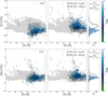 |
Fig. 24 Same as Fig. 22, but for [Cr/Fe] (top) and [Mn/Fe] (bottom). |
| In the text | |
Current usage metrics show cumulative count of Article Views (full-text article views including HTML views, PDF and ePub downloads, according to the available data) and Abstracts Views on Vision4Press platform.
Data correspond to usage on the plateform after 2015. The current usage metrics is available 48-96 hours after online publication and is updated daily on week days.
Initial download of the metrics may take a while.