| Issue |
A&A
Volume 665, September 2022
|
|
|---|---|---|
| Article Number | A33 | |
| Number of page(s) | 27 | |
| Section | Stellar atmospheres | |
| DOI | https://doi.org/10.1051/0004-6361/202142195 | |
| Published online | 08 September 2022 | |
Non-LTE abundance corrections for late-type stars from 2000 Å to 3 µm
I. Na, Mg, and Al★
1
Department of Astronomy, Stockholm University, AlbaNova University Center,
106 91
Stockholm, Sweden
e-mail: This email address is being protected from spambots. You need JavaScript enabled to view it.
2
Centre of Excellence for Astrophysics in Three Dimensions (ASTRO-3D),
Australia
3
Research School of Astronomy and Astrophysics, Australian National University,
ACT 2611,
Canberra, Australia
4
Department of Physics and Astronomy, Uppsala University,
Box 516,
75120
Uppsala, Sweden
5
Kapteyn Astronomical Institute, University of Groningen,
Landleven 12,
9747 AD
Groningen, The Netherlands
6
Isaac Newton Group,
Apartado 321,
38700
Santa Cruz de La Palma, Spain
7
Instituto de Astrofísicade Canarias,
38205
La Laguna, Tenerife, Spain
8
Departamento de Astrofísica, Universidad de La Laguna,
38206
La Laguna, Tenerife, Spain
9
Department of Astronomy and Space Sciences, Ege University,
35100
Bornova, İzmir, Turkey
10
Department of Astronomy and McDonald Observatory, The University of Texas,
Austin, TX
78712, USA
11
Centre for Astrophysics Research, Department of Physics, Astronomy and Mathematics, University of Hertfordshire,
Hatfield,
AL10 9AB, UK
Received:
10
September
2021
Accepted:
21
June
2022
Abstract
Context. It is well known that cool star atmospheres depart from local thermodynamic equilibrium (LTE). Making an accurate abundance determination requires taking those effects into account, but the necessary non-LTE (hereafter NLTE) calculations are often lacking.
Aims. Our goal is to provide detailed estimates of NLTE effects for FGK type stars for all spectral lines from the ultraviolet (UV) to the near infrared (NIR) that are potentially useful as abundance diagnostics. The first paper in this series focusses on the light elements Na, Mg, and Al.
Methods. The code PySME was used to compute curves of growth for 2158 MARCS model atmospheres in the parameter range 3800 < Teff < 8000 K, 0.0 < log(g) < 5.5, and −5 < [Fe/H] < +0.5. Two microturbulence values, 1 and 2 kms−1, and nine abundance points spanning −1 < [X/Fe] < 1 for element X, are used to construct individual line curves of growth by calculating the equivalent widths of 35 Na lines, 134 Mg lines, and 34 Al lines. The lines were selected in the wavelength range between 2000 Å and 3 µm.
Results. We demonstrate the power of the new grids with LTE and NLTE abundance analysis by means of equivalent width measurements of five benchmark stars; the Sun, Arcturus, HD 84937, HD 140283 and HD 122563. For Na, the NLTE abundances are lower than in LTE and show markedly reduced line-to-line scatter in the metal-poor stars. For Mg, we confirm previous reports of a significant ~0.25 dex LTE ionisation imbalance in metal-poor stars that is only slightly improved in NLTE (~0.18 dex). LTE abundances based on Mg II lines agree better with models of Galactic chemical evolution. For Al, NLTE calculations strongly reduce an ~0.6 dex ionisation imbalance seen in LTE for the metal-poor stars. The abundance corrections presented in this work are in good agreement with previous studies for the subset of lines that overlap, with the exception of strongly saturated lines.
Conclusions. A consensus between different abundance diagnostics is the most powerful tool available to stellar spectroscopists to assess the accuracy of the models. Here we report that NLTE abundance analysis in general leads to improved agreement, in particular for metal-poor stars. The residual scatter is believed to be caused mainly by unresolved blends and/or poor atomic data, with the notable exception of Mg, which calls for further investigation.
Key words: radiative transfer / stars: abundances / stars: atmospheres / stars: late-type / techniques: spectroscopic
Full Tables B.1, B.2, B.3 are only available at the CDS via anonymous ftp to cdsarc.u-strasbg.fr (130.79.128.5) or via http://cdsarc.u-strasbg.fr/viz-bin/cat/J/A+A/665/A33
© K. Lind et al. 2022
 Open Access article, published by EDP Sciences, under the terms of the Creative Commons Attribution License (https://creativecommons.org/licenses/by/4.0), which permits unrestricted use, distribution, and reproduction in any medium, provided the original work is properly cited.
This article is published in open access under the Subscribe-to-Open model. This email address is being protected from spambots. You need JavaScript enabled to view it. to support open access publication.
1 Introduction
The chemical composition of late-type stars is important for numerous fundamental scientific questions, including but not limited to; the origin of elements, the internal physics of stars, and the formation of matter and structure from dust and planets to star clusters and entire galaxies. The amount of data collected by stellar spectroscopic surveys has virtually exploded in the last decade, as part of the ‘industrial revolution’ of the field of Galactic archaeology (Nissen & Gustafsson 2018; Jofré et al. 2019; Helmi 2020). Millions of optical and near infrared (NIR) spectra are now available for analysis, and the precision of inferred stellar parameters and chemical abundances is determined jointly by the quality of the spectrum, the analysis method, and the physical accuracy of the stellar models.
Contrary to traditional spectroscopy which commonly relies on careful selection of the most reliable spectral lines, every pixel in entire spectra are now routinely analysed in the quest for higher abundance precision. This includes lines with uncertain atomic data, unknown blending properties, and departures from local thermodynamic equilibrium (LTE). The increasingly popular data-driven machine-learning techniques (e.g. Ness et al. 2015) may mitigate the known shortcomings of synthetic stellar spectra, but the model dependence still enters indirectly via the presumed known labels on which the method is trained.
It is in general of great importance to understand the departures from LTE, the so-called NLTE effects for all available abundance diagnostics. However, employing fully consistent NLTE radiative transfer for all elements in the calculation of model atmospheres and synthetic spectra is numerically far too demanding today, and as a result, a hybrid approach is commonly adopted. In the trace-element formalism, which we assume to hold in this study as well, the model atmosphere is computed in LTE and the NLTE solution, that is the statistical equilibrium, is found independently for one element at the time. As shown in multiple studies, the impact of NLTE effects on derived chemical abundances ranges from non-existent, to moderately influential, to very strongly influential at an order of magnitude (e.g. Asplund 2005; Mashonkina 2014; Amarsi et al. 2020). The outcome strongly depends on the conditions of the stellar atmosphere and the spectral line of interest and NLTE effects can therefore not be predicted a priori, but they must be computed for large grids of stars and lines.
Amarsi et al. (2020) recently published large grids of NLTE departure coefficients for 13 elements. The application of these grids for GALAH spectrum analysis revealed that NLTE abundance patterns reduce the star-to-star scatter compared to LTE and that effects on individual stars and lines range from strongly negative to moderately positive. That work was limited to the wavelength range and parameter range of the GALAH survey, but the departure coefficient grids have a much wider range of applicability. Here, we use the grids of Amarsi et al. (2020) to compute individual line synthetic spectra and curves of growth for the full FGK parameter space for as many lines as possible from the ultraviolet (UV) to the NIR. The first paper in this series studies the astrophysically very important light elements with atomic number Z = 11–13, that is Na, Mg, and Al.
Section 2 describes the observational data used to test the influence of the NLTE calculations. Section 3 describes the line selection and the calculation of LTE and NLTE synthetic spectra. Section 4 discusses the abundance results for the five benchmark stars, as well as compares them to previous NLTE work and to predictions from models of Galactic chemical evolution (GCE). Section 5 summarises our conclusions.
2 Observations
Table 1 lists the spectral atlases used for the five benchmark stars and their wavelength ranges. For the Sun and Arcturus, we used atlases created with the Fourier transform spectrograph (FTS) connected to the McMath/Pierce Solar telescope (Sun) and the Coude Feed/Mayall telescopes (Arcturus) at Kitt Peak National Observatory (Kurucz et al. 1984; Hinkle et al. 1995, 2000). For the infrared Sun, we also used the atlas created with another FTS connected to a telescope at the Institute for Astrophysics in Goettingen (IAG, Reiners et al. 2016). UV spectra were not used for the Sun and Arcturus because of the very strong line blending.
Ultraviolet spectra for the three metal-poor stars were retrieved from the ASTRAL catalogue (Ayres 2013), which has been created with the STIS spectrograph on the Hubble Space Telescope (HST). Optical spectra for the stars were retrieved from the archive of the Paranal Observatory Project (Bagnulo et al. 2003), collected with the UVES spectrograph on the VLT. For two stars, HD 140283 and HD 122563, we also include infrared spectra observed with the IGRINS instrument on the Harlan J. Smith Telescope at McDonald Observatory (Afşar et al. 2016).
3 Method
3.1 Line selection
The lines used for abundance determination were only selected based on the prospects of accurately measuring their equivalent widths in (some part of) the covered parameter space. Lines with very close blends by other species, either predicted as being present in the line list or visually evident from asymmetry in their line profile, were discarded. The line atomic data were retrieved from VALD1 using ‘extract all’ requests with default settings and including hyperfine splitting. The quality of available atomic data was not used as a selection criterion, and we advise the reader to take this into consideration when using the grids for abundance measurements.
The continuum was placed individually by eye for each line. For the Sun and Arcturus, the original normalisation of the spectral atlases was trusted to be accurate to within ~0.5%. The equivalent widths were derived with Gaussian line fits using the IDL SolarSoft library2. Multiple Gaussians were used to de-blend partially blended lines. For strong lines, we modelled the intrinsic Voigt profile using overlapping Gaussians of different depths and widths. The observed equivalent widths were computed by integrating the fitted line profiles and range from 1–1000 mÅ, which is a much more extended range than what is usually used for precision spectroscopy. The choice was made to demonstrate the influence of NLTE for as many lines as possible, but the average stellar abundances shown in the paper are based on a more restricted selection of lines. Good agreement was found when comparing to the equivalent widths found by direct integration of observed line profiles of the most unblended lines.
The equivalent width error was estimated as the sum of three components; the formal fitting uncertainty as determined with the Cayrel (1988) formula3, an additional 0.5% contribution stemming from the uncertainty in the continuum placement, and finally an error due to the blending fraction. The latter was estimated as 25% of the difference in equivalent width found by directly integrating the observed and synthetic spectra in regions where the synthetic flux is deeper than 0.1%. It should be clear to the reader that this is an empirical approach that mainly is useful to compare relative sizes of errors between lines. We omitted errors from other sources, such as atomic data.
3.2 Synthetic spectra
We computed LTE and NLTE synthetic spectra using the code PySME v0.4.142 (Wehrhahn 2021, and Wehrhahn et al., in prep.)4, a derivative of the classical and well-used Spectroscopy Made Easy code (Piskunov & Valenti 2017) with the IDL libraries re-implemented in python. A grid of 2158 MARCS models in the parameter range 3800 < Teff < 8000 K, 0.0 < log(g) < 5.5, and −5 < [Fe/H] < +0.5, was used assuming two values of microturbulence, 1 and 2 km s−1. The abundance −1 < [X/Fe] < 1 was varied in steps of 0.25 dex, resulting in nine abundance points for each element X. For each line, 38 844 LTE and NLTE synthetic spectra were thus computed. In total, approximately 200 000 CPU hours were used for the calculations.
The spectra were computed individually, on a wavelength grid spanning ±100 Å centred on each line. Wavelength points with normalised synthetic flux deeper than 0.99999 were saved and used to compute equivalent widths by integrating the flux profiles. NLTE abundance corrections were subsequently computed by interpolating the LTE and NLTE curves of growth to observed equivalent widths.
To synthesize lines in NLTE, PySME takes as input precomputed grids of departure coefficients, that is the ratios of NLTE/LTE level populations as a function of atmospheric depth. We used version 3 of the grids5 recently published by Amarsi et al. (2020) which were computed with the NLTE code Balder (Amarsi et al. 2018), and wee made sure that PySME uses the same grid of atmospheric models as Balder. The atomic models used by Amarsi et al. (2020) to compute departure coefficients were originally constructed for Na by Lind et al. (2011), Mg by Osorio et al. (2015), and Al by Nordlander & Lind (2017). The solar abundance scale adopted as a reference in this paper (Grevesse et al. 2007) is the same as that used in the MARCS models and the departure coefficient grid, specifically A(Na) = 6.17, A(Mg) = 7.53, A(Al) = 6.37, and A (Fe) = 7.45.
Overview of the spectral atlases used, listing instrument, telescope and wavelength region.
3.3 Stellar parameters
The stellar parameters adopted for the five benchmark stars are summarised in Table 2. The effective temperatures for stars other than the Sun have been computed by bolometric fluxes and limb-darkened angular diameters. In the case of Arcturus, HD 140283 and HD 122563, the diameters have been directly measured by interferometry, while for HD 84937, surface-brightness relations were used to obtain indirect diameters by Heiter et al. (2015). Surface gravities for the stars other than the Sun have been computed with the fundamental relation to mass and radius.
Metallicities and microturbulence values that can be found in the literature are based on different stellar parameters and/or different radiative transfer codes and/or different modelling assumptions (1D or 3D, LTE or NLTE). To ensure homogeneity, we therefore redetermined the metallicity, [Fe/H], and microturbulence values, ξ, for all the stars by measuring the strength of 11–14 Fe II lines and enforcing a flat trend in LTE abundance with equivalent width. The lines were selected based on the recommendations of Heiter et al. (2021) and are summarised in Table A.4. The atomic data can be found in Heiter et al. (2021). We note that the metallicity scale for the metal-poor stars is in agreement within 0.03 dex with the recent study by Amarsi et al. (2016), when limiting the comparison to Fe II lines modelled in 1D LTE.
Adopted stellar parameters.
4 Results and discussion
4.1 Na
Departures from LTE for Na I have been studied extensively, starting with pioneering efforts half a century ago (Athay & Can-field 1969; Gehren 1975), while more recent references can be found in Lind et al. (2011) and Alexeeva et al. (2014). The dominant NLTE effect in Na I is darkening of the cores of strong lines, caused by photon suction. NLTE corrections based on equivalent-width measurements are negative and can reach more than −0.5 dex at full saturation. Due to the sparsity of lines of this alkali in late-type spectra, saturated lines are sometimes the only available diagnostic. One extreme example is the use of the Na D lines in metal-poor horizontal branch stars, with NLTE corrections as large as −0.9 dex (Marino et al. 2011).
Grids of NLTE corrections for Na I lines have been published by several authors, all solving the restricted NLTE problem for trace elements in 1D LTE stellar atmospheres:
Mashonkina et al. (2000), for 14 optical/NIR lines <1.3 µm
Takeda et al. (2003), for eight optical lines
Shi et al. (2004), for eight optical lines
Andrievsky et al. (2007), for the Na D lines
Lind et al. (2011), for 11 optical/NIR lines <1.1 µm
This study includes 35 Nal UV-NIR lines.
The optical wavelength band has traditionally dominated studies of Galactic archaeology, but with the advent of high-resolution multi-object spectrographs such as APOGEE (Majewski et al. 2017), the NIR is attracting more and more attention. To our knowledge, the first work to study NLTE effects on the 1.6 µm Na I lines in the H band is Osorio et al. (2020), but as their method is based on spectrum synthesis, they did not publish a grid of NLTE corrections. In this study, we compute and make available corrections for 35 Na I lines between 3302 Å and 2.59 µm, thus extending the availability of such data both into the UV and further into the NIR. All oscillator strengths are of a high quality, with A-B ratings in NIST. New broadening data due to H collisions were computed for three NIR lines around 2.2 µm using the Anstee, Barklem & O’Mara theory (Anstee & O’Mara 1995; Barklem & O’Mara 1997); in the case of the 2.14 micron line the upper state is a Rydberg state and an estimate of the broadening was made following Osorio et al. (2015) (see also Hoang-Binh & van Regemorter 1995).
Figure 1 shows the Na LTE and NLTE abundances determined for the five benchmark stars in our sample. The abundance and line data can be found in Table A.1. For the Sun and Arcturus, 13–14 lines are available in the optical (<1.1 µm) and two to four lines are available around 2 µm. NLTE effects are moderate, lowering the average abundance by −0.1 dex. The line-to-line scatter in the Sun and Arcturus is slightly reduced.
In the metal-poor stars, only three to five lines are strong enough to be measured. The NLTE abundances are lower by −0.2 dex on average, and a drastically reduced scatter is seen for all stars. This is primarily driven by the strong negative NLTE abundance correction for the Na D lines. Overall, acceptable agreement is seen across UV, optical, and NIR wavelength ranges, when available.
Figure 2 illustrates how the typical NLTE effect for unsaturated lines vary as a function of stellar parameters. Four different stellar types are shown, one red giant, one horizontal branch star, one cool dwarf and a turn-off star. We see that NLTE corrections for unsaturated lines are typically small and negative, −0.1 dex to −0.2 dex, everywhere in the displayed parameter space. Only at the very lowest metallicities is a slight, positive upturn seen.
4.2 Mg
Magnesium is typically twenty times more abundant than its two neighbours in the periodic table, and many more lines are also available as abundance diagnostics in late-type stars. Lines of both neutral and singly ionised Mg can be measured down to low metallicity. The first NLTE investigation again dates back to Athay & Canfield (1969) and many have followed since then. Several studies have determined NLTE line formation for a specific sample of stars, including Andrievsky et al. (2010), Bergemann et al. (2017b), and Sitnova et al. (2019), but only a select number of studies have provided NLTE abundance corrections in tabulated form:
Shimanskaya et al. (2000) for five optical lines
Merle et al. (2011) for 16 optical/NIR lines <1.2 µm
Bergemann et al. (2015) for two NIR lines
Osorio & Barklem (2016) for 19 optical/NIR lines <2.1 µm
This study includes 134 Mg I UV-NIR lines.
For Mg I, NLTE effects are typically small and can be both positive and negative, depending on the competing effects of over-ionisation and photon suction. Because the model atom (Osorio et al. 2015) lacks collisions between hydrogen atoms and Mg II, we suspect that NLTE effects are overestimated for Mg II and assume that LTE is a better approximation.
Many Mg I lines have oscillator strengths with large uncertainties in the VALD3 database, with corresponding entries in NIST flagged as C (≤25%) or lower. The transition probabilities have been greatly improved with the combined experimental and theoretical study by Pehlivan Rhodin et al. (2017), and we used this reference when possible. In Fig. 3, we show Mg I-based abundances determined with Pehlivan Rhodin et al. (2017) values with filled black bullets and other Mg I lines with open bullets. Red bullets mark Mg II lines. The line-by-line abundances are listed in Table A.2.
Between 26 and 55 lines were used for abundance determination of the five benchmark stars, which is significantly more than previous studies. The average NLTE effect for Mg I lines is –0.02 dex in the Sun, –0.10 dex in Arcturus and +0.08 dex for the metal-poor turn-off and subgiant. As the plots clearly show, the line-to-line scatter is smaller when only considering lines that have high-quality transition probabilities. The line-to-line scatter for Mg I lines is not significantly affected by NLTE. In both LTE and NLTE there is a tendency for saturated lines to give lower abundance. In particular, the saturated lines <3000 Å give abundances that are significantly lower than the average. The mean abundances and standard deviations shown in Fig. 3 are based on weak to moderately strong lines with good oscillator strengths, as indicated in the figure caption.
In the literature, Mg II lines are not commonly used for abundance analysis, and it is particularly important to stress the significant ionisation imbalance found for HD 84937 and HD 140283, which is of the order of −0.25 dex in LTE and only mildly reduces to −0.18 dex in NLTE. This confirms the results of Alexeeva et al. (2018) who report a clear discrepancy between abundances based on Mg II 4481 Å and the average of Mg I lines for the same two stars. Here, we add two bluer Mg II lines that support the high abundance found with 4481 Å , and hence undetected blends in the latter is probably not the underlying cause. At this point, we may only speculate along the same lines as Alexeeva et al. (2018) that 3D effects may be to blame for the ionisation imbalance, and we plan to address Mg with full 3D NLTE modelling in a future study. However, according to Bergemann et al. (2017a), NLTE abundances computed based on Mg I lines using so-called < 3D > models, which are spatial and temporal averages of full 3D simulations, are not substantially higher than 1D-based abundances. We cannot rule out that our atomic model or modelling assumptions underestimate(s) the NLTE effects in Mg I in both 1D and 3D, perhaps because the trace element method neglects possible feedback effects from other elements (Osorio et al. 2020).
Looking at a more extended parameter space, Fig. 2 shows that our predicted Mg abundance corrections for unsaturated lines show a simple trend that is increasingly positive towards lower metallicites. At the lowest metallicities, giants are predicted to depart from LTE by ~ 0.3 dex.
4.3 Al
Non-local thermodynamic equilibrium spectroscopic analysis for Al I was mainly pioneered by Baumueller & Gehren (1996, 1997), highlighting the strong over-ionisation in metal-poor stars. Later important work include that of Gehren et al. (2004, 2006) and Andrievsky et al. (2008), which however did not compute grids of abundance corrections to use for quantitative spectroscopy. The first such grids were published by:
Menzhevitski et al. (2012) for nine optical lines
Mashonkina et al. (2016) for six optical lines
Nordlander & Lind (2017) 26 UV-NIR lines
This study includes 43 AlI and three AlII UV-NIR lines.
The number of Al lines available for abundance analysis in the five benchmark stars is similar to Na, that is to say around 18 in total at high metallicity, but there is only a select number at low metallicity. The main reason why Al is, nevertheless, a less well studied element is because the detectable lines at low metallicity fall below 4000 Å or in the H band, while Na has strong lines in the optical. The NLTE effects are also similar at high metallicity, with photon suction causing increasingly negative corrections as the lines become saturated. At low metallicity, however, the overionisation of neutral Al is much stronger than for both Na and Mg and the Al I NLTE abundance corrections are therefore positive, that is of the order of order +0.4 dex in the two unevolved stars.
As shown in Fig. 4 and Table A.3, the line-to-line scatter for neutral lines is not strongly affected overall, but we note that for Arcturus, NLTE analysis brings the strong NIR lines into agreement with the optical lines. For HD 140283 and HD 84937, we can investigate the ionisation balance using Al II 2669 Å which forms close to LTE and has a high-quality gf value from Träbert et al. (1999). For the neutral lines, we adopted the theoretical gf-values available in TOPbase (Mendoza et al. 1995). We find that the abundance determined from the singly ionised line is higher than the neutral lines by 0.6 dex in LTE and 0.2 dex in NLTE. Given the lower number of lines and their scatter, we consider the ionisation imbalance in NLTE for Al less alarming than for Mg. The ionisation balance of Al was first investigated by Roederer & Lawler (2021) for a sample of 11 metal-poor stars, finding a 0.40.9 dex discrepancy between the ionisation stages in LTE. They further note that the NLTE corrections provided by Nordlander & Lind (2017) resolved the imbalance.
Figure 2 further emphasises how important NLTE analysis is for Al abundances of metal-poor stars, with corrections of up to 0.8 dex for giants in the metal-poor end of the studied grid. Cool dwarf stars show a different behaviour, with negative corrections in the metallicity range where unsaturated optical lines are detectable.
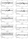 |
Fig. 1 Na abundances derived from neutral lines with Wλ,red < 3 × 10⁻⁵ (black bullets) and Wλ,red < 3 × 10⁻⁵ (open bullets) in LTE (left) and NLTE (right). The horizontal lines and grey-shaded regions correspond to the mean and one sigma standard deviation of the lines, respectively. |
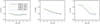 |
Fig. 2 Average NLTE effect for optical unsaturated lines (3000–10 000 Å and Wλ,red < 3 × 10⁻⁵) as a function of metallicity. Four different stellar types are shown with stellar parameters as indicated by the legend. Only those data points that have <0.1 dex standard deviation among the spectral lines used to form the mean are retained. |
4.4 Comparison to previous work
In Sects. 4.1–4.3, we have listed several literature studies that present NLTE abundance corrections for Na, Mg, and Al for a grid of 1D model atmospheres. As a whole, they present a variety of different atmospheric and atomic models, as well as different codes for statistical equilibrium and radiative transfer calculations. What all three elements have in common is that quantum mechanical data for collisions with neutral hydrogen have become available in the last decade (Belyaev et al. 2010; Belyaev 2013; Barklem et al. 2010, 2012), thereby removing a notorious and large source of uncertainty in the atomic model. The impact of the new data on stellar abundances with respect to the previously adopted Drawin formula (Drawin 1968, 1969) have been extensively described (e.g. Mashonkina 2013; Mashonkina et al. 2016; Ezzeddine et al. 2018). Here, we limit the comparison to work that use, with minor modifications, the same atomic model and MARCS atmospheric models as was used by Amarsi et al. (2020) to compute the departure coefficients adopted in this work. The comparison therefore mainly highlights differences caused by choice of code to solve the statistical equilibrium and compute the synthetic spectrum. All previous work shown in Fig. 5 used MULTI2.3 (Carlsson 1992) for both purposes, while we have used Balder to establish the statistical equilibrium and PySME to compute the curves of growth.
In Fig. 5 we compare our results to Lind et al. (2011) for Na, Osorio & Barklem (2016) for Mg, and Nordlander & Lind (2017) for Al. The agreement for the majority of lines is good, but there are several notable exceptions, in particular for saturated lines with reduced equivalent widths in the range Wλ,red = (1 – 3) × 10−5. For such lines, our new corrections can be significantly different, and usually more negative. The effect is strongest for the two giants in our sample. To attempt to trace the origin of these differences, we have investigated the curves of growth in some more detail.
Figure 6 illustrates how the line strength grows in LTE and NLTE for three lines that are saturated in Arcturus; Na 8183 Å, Mg 7692 Å, and Al 21164 Å. Our new curves of growth computed with Balder/PySME are compared to ones computed with MULTI2.3. We see in all three cases that the agreement between LTE curves and NLTE curves at a given line strength is similar, that is, the new results deviate in unison from the old ones. This leads us to conclude that the differences do not originate in different solutions to the statistical equilibrium, but from the calculation of the LTE and NLTE line and continuous opacity by MULTI2.3 and PySME.
We note the flattening of the curves for Mg that is evident at high abundance, where the equivalent width appears insensitive to increased abundance. In fact, this is a behaviour seen for all Mg lines, and at [Mg/Fe] > 1, the curves can even have a negative slope. This counter-intuitive behaviour can be explained by the importance of Mg as electron donor. As the abundance increases, the continuous opacity which is dominated by H− also increases, reducing spectral line strengths. If the atmospheric models had been recomputed consistently with the adopted chemical composition, the trends may well have looked different. The dotted line marked ‘Consistent’ in the Mg panel illustrates this by showing a smaller part of the LTE curve of growth for which we have used alpha-negative ([α/Fe] = −0.4), alpha-poor ([α/Fe] = 0.0) and alpha-enhanced MARCS models ([α/Fe] = 0.4) instead of the standard composition ([α/Fe] = 0.2 at [Fe/H] = −0.5). This curve crosses the reference and inconsistent LTE curve of growth (black solid) at [α/Fe] = 0.2 as expected, but it does not show the same flattening at higher abundance. We therefore advise caution in the use of the grids at the upper and lower end of the abundance range.
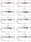 |
Fig. 3 Mg abundances derived from neutral lines with Wλ,red < 3 × 10⁻⁵ and high-quality gf values (black bullets), from neutral lines with Wλ,red < 3 × 10⁻⁵ and/or low-quality gf-values (open bullets), and from singly ionised lines (red bullets) in LTE (left) and NLTE (right). The black horizontal lines and grey-shaded regions correspond to the mean and one sigma standard deviation of the lines marked with filled black bullets. The red horizontal lines correspond to the mean of the singly ionised lines. |
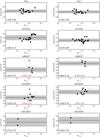 |
Fig. 4 Al abundances derived from neutral lines with Wλ,red < 3 × 10⁻⁵ and high-quality gf values (black bullets), from neutral lines with Wλ,red < 3 × 10⁻⁵ and/or low-quality gf values (open bullets), and from singly ionised lines (red bullets) in LTE (left) and NLTE (right). The black horizontal lines and grey-shaded regions correspond to the mean and one sigma standard deviation of the lines marked with filled black bullets. |
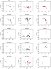 |
Fig. 5 New NLTE corrections compared to previous work. Black bullets represent the results of this study and red open squares the results of Lind et al. (2011) for Na, Osorio & Barklem (2016) for Mg, and Nordlander & Lind (2017) for Al. Vertical lines connect lines in common between the studies. |
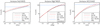 |
Fig. 6 Examples of LTE (black) and NLTE (red) curves of growth for spectral lines of three different elements in Arcturus. Solid lines represent the results of this work and dashed lines correspond to the results of Lind et al. (2011) for Na, Osorio & Barklem (2016) for Mg, and Nordlander & Lind (2017) for Al. The black dotted line in the middle panel has been computed with model atmospheres that have consistent [α/Fe] ratios as explained in the text. |
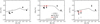 |
Fig. 7 Comparison of the abundances found for the benchmark stars analysed in this paper (bullets) to the Galactic chemical evolution model of Kobayashi et al. (2020). The Sun is marked at the origin. |
4.5 Comparison to Galactic chemical evolution models
All three elements studied here are primarily forged in massive stars during hydrostatic carbon burning and returned to the interstellar medium by core-collapse supernovae (SN) and hyper-novae (HN) (Nomoto et al. 2013; Johnson 2019). The α-element
Mg is predicted to form a plateau value in [Mg/Fe] at low metallicity and decreasing ratio when supernovae of type 1a (SNIa) start contributing with relatively more Fe. The metallicity at which this decrease occurs is environment dependent, because the star formation history depicts how much Fe had time to form via SN and HN prior to the delayed onset of SNIa. In the Milky Way, the ‘knee’ in the [α/Fe] is located at [Fe/H] = −1.
However, Na and Al yields, also depend on the available neutron excess and thus on the metallicity of the massive star progenitor. The [Na/Fe] and [Al/Fe] ratios are therefore predicted to increase with increasing metallicity, until SNIa start contributing and reduce the ratios. For completeness, it should be mentioned that all three elements have minor contributions from the NeNa and MgAl nucleosynthesis channels that coexist with the CNO cycle of hydrogen at a high temperature and they are therefore frequently studied, for example, to characterize the different generations of stellar populations of globular clusters (Bastian & Lardo 2018).
Our sample of stars is much too small to draw conclusions concerning the success or failure of GCE models. However, the NLTE effects we have demonstrated in this paper are systematic and have a similar effect on stars with similar stellar parameters. It is therefore of interest to compare models and observations to gauge the possible impact for larger samples. Figure 7 shows how the abundances compare to the GCE model of Kobayashi et al. (2020).
As seen in Fig. 7, the mean [Mg/Fe] abundance for metal-poor stars is 0.27, based on Mg I lines (NLTE) and 0.46, based on Mg II lines (LTE). Interestingly, the latter is in significantly better agreement with the plateau value of the model. Kobayashi et al. (2020) report on a similar offset using NLTE literature studies of neutral Mg lines. On the other hand, in the metal-poor regime the GCE model is in excess of the NLTE abundances for neutral lines by ~0.2 dex for all three elements studied here, which may point to a different explanation, such as a change in the relative abundance of alpha elements due to a change in nuclear reaction rates and/or stellar mass loss (due to rotation and/or binary interaction, see Kobayashi et al. 2006). We further note that the predicted [(Na,Al)/Fe] ratios could become even higher for GCE models that are based on yields taking the effects of stellar rotation into account.
With such few observational data points as shown in Fig. 7, these are merely speculations, and we call for a larger investigation of the Mg (and Al) ionisation balance to be performed over a large range of metallicities. This is particularly relevant and urgent because these abundances are frequently used to trace the origin of halo stars, and to differentiate between ones that formed in situ at high values compatible with the Galactic thick disk and low values that are interpreted as a sign of accretion from lower-mass systems (e.g. Nissen & Gustafsson 2018; Helmi 2020).
5 Conclusions
There is a great need to understand how departures from LTE affect chemical abundance determination for all absorption lines that are detectable in stellar spectra. In this work we have computed NLTE abundance corrections with PySME for 2-5 times more lines for Na, Mg, and Al, compared to what is available in the literature. We show that NLTE analysis generally leads to improved consistency between abundance diagnostics for five benchmark stars and that our NLTE corrections are compatible with previous studies that used the same atomic and atmospheric models, except for strongly saturated lines for which NLTE corrections are very sensitive to the choice of the radiative transfer code.
Our conclusions for the different elements are as follows:
The NLTE corrections for Na I are increasingly negative with line strength until the point of maximum saturation. Unsaturated optical lines nearly always have moderately negative corrections. NLTE abundances for different lines are significantly more homogeneous compared to LTE for metal-poor stars.
In addition, Mg I NLTE corrections are mostly small in absolute value and can be both positive and negative. The ionisation balance is met in the Sun, assuming Mg II lines form in LTE, but not in metal-poor unevolved stars. The 0.2 dex NLTE ionisation imbalance for HD 84937 and HD 140283 can depend on shortcomings in the methodology or the atomic or atmospheric model and it must be further investigated. Magnesium is an important electron donor, and indirect effects on the continuous opacity may lead to unphysical growth curves when the atmospheric model is not consistently updated. Caution is advised when using ourdata for abundances that are different from the standard MARCS composition.
Furthermore, Al I NLTE corrections for metal-rich stars are increasingly negative with line strength until the point of maximum saturation. Unsaturated, optical lines display trends of sharply increasing positive corrections towards lower metallicity for turn-off stars and giants. NLTE analysis strongly improves the ionisation balance in the metal-poor regime.
The grids of LTE and NLTE equivalent widths are available in Tables B.1-B.3. The synthetic equivalent widths can be used to compute LTE and NLTE abundances for stars in the parameter space covered by the model grids.
Acknowledgements
K.L. and M.M. acknowledge funds from the European Research Council (ERC) under the European Union’s Horizon 2020 research and innovation programme (Grant agreement No. 852977). The computations were enabled by resources provided by the Swedish National Infrastructure for Computing (SNIC) at UPPMAX, partially funded by the Swedish Research Council through grant agreement no. 2018-05973. C.K. acknowledges funding from the UK Science and Technology Facility Council (STFC) through grant ST/M000958/1 and ST/V000632/1. This work is supported by the Swedish Research Council through an individual project grant with contract No. 202003404. K.L. and P.B. acknowledge support by the Knut and Alice Wallenberg Foundation.
Appendix A Line data
This appendix contains four tables, one for each element Na, Mg, Al, and Fe, containing line atomic data as well as equivalent widths and abundances for the benchmark stars. Specifically, for each spectral line, the tables list the species, the air wavelength in Å, the lower-level excitation energy in eV, the log(gf) value, and the Van der Waals broadening parameter (VdW) that represents the logarithm of the FWHM per unit pertuber number density at 10,000 K, given in [rad s−1 cm−3]. If no data are present in this column, the Unsöld broadening recipe was used. For each line, there are two or three lines with stellar data which should be interpreted as the equivalent width in mÅ (first row), the LTE abundance (second row), and NLTE abundance (third row, not available for Mg II lines or Fe II lines).
Na line list
Mg line list
Al line list
Fe line list
Appendix B Grids of equivalent widths
This appendix contains three tables with LTE and non-LTE equivalent widths for Na, Mg and Al that can be used to compute LTE and NLTE abundances by interpolation to observationally inferred stellar parameters and equivalent widths. The full tables are available in electronic form at the CDS.
Equivalent widths for Na lines
Equivalent widths for Mg lines
Equivalent widths for Al lines
References
- Afşar, M., Sneden, C., Frebel, A., et al. 2016, ApJ, 819, 103 [Google Scholar]
- Alexeeva, S. A., Pakhomov, Y. V., & Mashonkina, L. I. 2014, Astron. Lett., 40, 406 [NASA ADS] [CrossRef] [Google Scholar]
- Alexeeva, S., Ryabchikova, T., Mashonkina, L., & Hu, S. 2018, ApJ, 866, 153 [Google Scholar]
- Amarsi, A. M., Lind, K., Asplund, M., Barklem, P. S., & Collet, R. 2016, MNRAS, 463, 1518 [NASA ADS] [CrossRef] [Google Scholar]
- Amarsi, A. M., Nordlander, T., Barklem, P. S., et al. 2018, A&A, 615, A139 [NASA ADS] [CrossRef] [EDP Sciences] [Google Scholar]
- Amarsi, A. M., Lind, K., Osorio, Y., et al. 2020, A&A, 642, A62 [EDP Sciences] [Google Scholar]
- Andrievsky, S. M., Spite, M., Korotin, S. A., et al. 2007, A&A, 464, 1081 [NASA ADS] [CrossRef] [EDP Sciences] [Google Scholar]
- Andrievsky, S. M., Spite, M., Korotin, S. A., et al. 2008, A&A, 481, 481 [NASA ADS] [CrossRef] [EDP Sciences] [Google Scholar]
- Andrievsky, S. M., Spite, M., Korotin, S. A., et al. 2010, A&A, 509, A88 [NASA ADS] [CrossRef] [EDP Sciences] [Google Scholar]
- Anstee, S. D., & O’Mara, B. J. 1995, MNRAS, 276, 859 [Google Scholar]
- Asplund, M. 2005, ARA&A, 43, 481 [Google Scholar]
- Athay, R. G., & Canfield, R. C. 1969, ApJ, 156, 695 [NASA ADS] [CrossRef] [Google Scholar]
- Ayres, T. R. 2013, Astron. Nachr., 334, 105 [NASA ADS] [CrossRef] [Google Scholar]
- Bagnulo, S., Jehin, E., Ledoux, C., et al. 2003, The Messenger, 114, 10 [Google Scholar]
- Barklem, P. S., & Aspelund-Johansson, J. 2005, A&A, 435, 373 [NASA ADS] [CrossRef] [EDP Sciences] [Google Scholar]
- Barklem, P. S., & O’Mara, B. J. 1997, MNRAS, 290, 102 [Google Scholar]
- Barklem, P. S., Piskunov, N., & O’Mara, B. J. 2000, A&AS, 142, 467 [NASA ADS] [CrossRef] [EDP Sciences] [Google Scholar]
- Barklem, P. S., Belyaev, A. K., Dickinson, A. S., & Gadéa, F. X. 2010, A&A, 519, A20 [NASA ADS] [CrossRef] [EDP Sciences] [Google Scholar]
- Barklem, P. S., Belyaev, A. K., Spielfiedel, A., Guitou, M., & Feautrier, N. 2012, A&A, 541, A80 [NASA ADS] [CrossRef] [EDP Sciences] [Google Scholar]
- Bastian, N., & Lardo, C. 2018, ARA&A, 56, 83 [Google Scholar]
- Baumueller, D., & Gehren, T. 1996, A&A, 307, 961 [NASA ADS] [Google Scholar]
- Baumueller, D., & Gehren, T. 1997, A&A, 325, 1088 [NASA ADS] [Google Scholar]
- Belyaev, A. K. 2013, A&A, 560, A60 [NASA ADS] [CrossRef] [EDP Sciences] [Google Scholar]
- Belyaev, A. K., Barklem, P. S., Dickinson, A. S., & Gadéa, F. X. 2010, Phys. Rev. A, 81, 032706 [NASA ADS] [CrossRef] [Google Scholar]
- Bergemann, M., Kudritzki, R.-P., Gazak, Z., Davies, B., & Plez, B. 2015, ApJ, 804, 113 [NASA ADS] [CrossRef] [Google Scholar]
- Bergemann, M., Collet, R., Amarsi, A. M., et al. 2017a, ApJ, 847, 15 [NASA ADS] [CrossRef] [Google Scholar]
- Bergemann, M., Collet, R., Schönrich, R., et al. 2017b, ApJ, 847, 16 [Google Scholar]
- Carlsson, M. 1992, ASP Conf. Ser., 26, 499 [Google Scholar]
- Cayrel, R. 1988, IAU Symp. 132, 345 [NASA ADS] [Google Scholar]
- Drawin, H.-W. 1968, Z. Phys., 211, 404 [NASA ADS] [CrossRef] [Google Scholar]
- Drawin, H. W. 1969, Z. Phys., 225, 483 [CrossRef] [Google Scholar]
- Ezzeddine, R., Merle, T., Plez, B., et al. 2018, A&A, 618, A141 [NASA ADS] [CrossRef] [EDP Sciences] [Google Scholar]
- Gehren, T. 1975, A&A, 38, 289 [Google Scholar]
- Gehren, T., Liang, Y. C., Shi, J. R., Zhang, H. W., & Zhao, G. 2004, A&A, 413, 1045 [NASA ADS] [CrossRef] [EDP Sciences] [Google Scholar]
- Gehren, T., Shi, J. R., Zhang, H. W., Zhao, G., & Korn, A. J. 2006, A&A, 451, 1065 [NASA ADS] [CrossRef] [EDP Sciences] [Google Scholar]
- Grevesse, N., Asplund, M., & Sauval, A. J. 2007, Space Sci. Rev., 130, 105 [Google Scholar]
- Heiter, U., Jofré, P., Gustafsson, B., et al. 2015, A&A, 582, A49 [NASA ADS] [CrossRef] [EDP Sciences] [Google Scholar]
- Heiter, U., Lind, K., Bergemann, M., et al. 2021, A&A, 645, A106 [EDP Sciences] [Google Scholar]
- Helmi, A. 2020, ARA&A, 58, 205 [Google Scholar]
- Hinkle, K., Wallace, L., & Livingston, W. 1995, PASP, 107, 1042 [Google Scholar]
- Hinkle, K., Wallace, L., Valenti, J., & Harmer, D. 2000, Visible and Near Infrared Atlas of the Arcturus Spectrum 3727-9300 A (USA: Astronomical Society of the Pacific) [Google Scholar]
- Hoang-Binh, D., & van Regemorter, H. 1995, J. Phys. B Atm. Mol. Phys., 28, 3147 [NASA ADS] [CrossRef] [Google Scholar]
- Jofré, P., Heiter, U., & Soubiran, C. 2019, ARA&A, 57, 571 [Google Scholar]
- Johnson, J. A. 2019, Science, 363, 474Karovicova, I., White, T. R., Nordländer, T., et al. 2020, A&A, 640, A25 [Google Scholar]
- Kobayashi, C., Umeda, H., Nomoto, K., Tominaga, N., & Ohkubo, T. 2006, ApJ, 653, 1145 [NASA ADS] [CrossRef] [Google Scholar]
- Kobayashi, C., Karakas, A. I., & Lugaro, M. 2020, ApJ, 900, 179 [Google Scholar]
- Kurucz, R. L., & Peytremann, E. 1975, SAO Sp. Rep., 362, 1 [Google Scholar]
- Kurucz, R. L., Furenlid, I., Brault, J., & Testerman, L. 1984, Solar Flux Atlas from 296 to 1300 nm (Cambridge: Cambridge University Press) [Google Scholar]
- Lind, K., Asplund, M., Barklem, P. S., & Belyaev, A. K. 2011, A&A, 528, A103 [NASA ADS] [CrossRef] [EDP Sciences] [Google Scholar]
- Majewski, S. R., Schiavon, R. P., Frinchaboy, P. M., et al. 2017, AJ, 154, 94 [NASA ADS] [CrossRef] [Google Scholar]
- Marino, A. F., Villanova, S., Milone, A. P., et al. 2011, ApJ, 730, L16 [NASA ADS] [CrossRef] [Google Scholar]
- Mashonkina, L. 2013, A&A, 550, A28 [NASA ADS] [CrossRef] [EDP Sciences] [Google Scholar]
- Mashonkina, L. 2014, IAU Symp., 298, 355 [NASA ADS] [Google Scholar]
- Mashonkina, L. I., Shimanskii, V. V., & Sakhibullin, N. A. 2000, Astron. Rep., 44, 790 [NASA ADS] [CrossRef] [Google Scholar]
- Mashonkina, L. I., Belyaev, A. K., & Shi, J. R. 2016, Astron. Lett., 42, 366 [NASA ADS] [CrossRef] [Google Scholar]
- Meléndez, J., & Barbuy, B. 2009, A&A, 497, 611 [NASA ADS] [CrossRef] [EDP Sciences] [Google Scholar]
- Mendoza, C., Eissner, W., LeDourneuf, M., & Zeippen, C. J. 1995, J. Phys. B Atm. Mol. Phys., 28, 3485 [NASA ADS] [CrossRef] [Google Scholar]
- Menzhevitski, V. S., Shimansky, V. V., & Shimanskaya, N. N. 2012, Astrophys. Bull., 67, 294 [NASA ADS] [CrossRef] [Google Scholar]
- Merle, T., Thévenin, F., Pichon, B., & Bigot, L. 2011, MNRAS, 418, 863 [NASA ADS] [CrossRef] [Google Scholar]
- Ness, M., Hogg, D. W., Rix, H. W., Ho, A. Y. Q., & Zasowski, G. 2015, ApJ, 808, 16 [NASA ADS] [CrossRef] [Google Scholar]
- Nissen, P. E., & Gustafsson, B. 2018, A&ARv, 26, 6 [Google Scholar]
- Nomoto, K., Kobayashi, C., & Tominaga, N. 2013, ARA&A, 51, 457 [CrossRef] [Google Scholar]
- Nordlander, T., & Lind, K. 2017, A&A, 607, A75 [NASA ADS] [CrossRef] [EDP Sciences] [Google Scholar]
- Osorio, Y., & Barklem, P. S. 2016, A&A, 586, A120 [NASA ADS] [CrossRef] [EDP Sciences] [Google Scholar]
- Osorio, Y., Barklem, P. S., Lind, K., et al. 2015, A&A, 579, A53 [NASA ADS] [CrossRef] [EDP Sciences] [Google Scholar]
- Osorio, Y., Allende Prieto, C., Hubeny, I., Mészáros, S., & Shetrone, M. 2020, A&A, 637, A80 [NASA ADS] [CrossRef] [EDP Sciences] [Google Scholar]
- Pehlivan Rhodin, A., Hartman, H., Nilsson, H., & Jönsson, P. 2017, A&A, 598, A102 [NASA ADS] [CrossRef] [EDP Sciences] [Google Scholar]
- Piskunov, N., & Valenti, J. A. 2017, A&A, 597, A16 [NASA ADS] [CrossRef] [EDP Sciences] [Google Scholar]
- Prša, A., Harmanec, P., Torres, G., et al. 2016, AJ, 152, 41 [Google Scholar]
- Raassen, A. J. J., & Uylings, P. H. M. 1998, A&A, 340, 300 [Google Scholar]
- Ralchenko, Y., Kramida, A., Reader, J., & NIST ASD Team. 2010, NIST Atomic Spectra Database (ver. 4.0.0), http://physics.nist.gov/asd [Google Scholar]
- Reiners, A., Mrotzek, N., Lemke, U., Hinrichs, J., & Reinsch, K. 2016, A&A, 587, A65 [NASA ADS] [CrossRef] [EDP Sciences] [Google Scholar]
- Roederer, I. U., & Lawler, J. E. 2021, ApJ, 912, 119 [NASA ADS] [CrossRef] [Google Scholar]
- Schaefer, A. R. 1971, ApJ, 163, 411 [NASA ADS] [CrossRef] [Google Scholar]
- Shi, J. R., Gehren, T., & Zhao, G. 2004, A&A, 423, 683 [NASA ADS] [CrossRef] [EDP Sciences] [Google Scholar]
- Shimanskaya, N. N., Mashonkina, L. I., & Sakhibullin, N. A. 2000, Astron. Rep., 44, 530 [NASA ADS] [CrossRef] [Google Scholar]
- Sitnova, T. M., Mashonkina, L. I., Ezzeddine, R., & Frebel, A. 2019, MNRAS, 485, 3527 [NASA ADS] [CrossRef] [Google Scholar]
- Takeda, Y., Zhao, G., Takada-Hidai, M., et al. 2003, Chinese J. Astron. Astrophys., 3, 316 [NASA ADS] [CrossRef] [Google Scholar]
- Träbert, E., Wolf, A., Linkemann, J., & Tordoir, X. 1999, J. Phys. B Atm. Mol. Opt. Phys., 32, 537 [CrossRef] [Google Scholar]
- Wehrhahn, A. 2021, https://doi.org/10.5281/zenodo.4537913 [Google Scholar]
1.5/(S/N) ×  , where S/N is the average flux error, λ the wavelength, δλ the pixel size, and R the spectral resolution.
All Tables
Overview of the spectral atlases used, listing instrument, telescope and wavelength region.
All Figures
|
Fig. 1 Na abundances derived from neutral lines with Wλ,red < 3 × 10⁻⁵ (black bullets) and Wλ,red < 3 × 10⁻⁵ (open bullets) in LTE (left) and NLTE (right). The horizontal lines and grey-shaded regions correspond to the mean and one sigma standard deviation of the lines, respectively. |
| In the text | |
|
Fig. 2 Average NLTE effect for optical unsaturated lines (3000–10 000 Å and Wλ,red < 3 × 10⁻⁵) as a function of metallicity. Four different stellar types are shown with stellar parameters as indicated by the legend. Only those data points that have <0.1 dex standard deviation among the spectral lines used to form the mean are retained. |
| In the text | |
|
Fig. 3 Mg abundances derived from neutral lines with Wλ,red < 3 × 10⁻⁵ and high-quality gf values (black bullets), from neutral lines with Wλ,red < 3 × 10⁻⁵ and/or low-quality gf-values (open bullets), and from singly ionised lines (red bullets) in LTE (left) and NLTE (right). The black horizontal lines and grey-shaded regions correspond to the mean and one sigma standard deviation of the lines marked with filled black bullets. The red horizontal lines correspond to the mean of the singly ionised lines. |
| In the text | |
|
Fig. 4 Al abundances derived from neutral lines with Wλ,red < 3 × 10⁻⁵ and high-quality gf values (black bullets), from neutral lines with Wλ,red < 3 × 10⁻⁵ and/or low-quality gf values (open bullets), and from singly ionised lines (red bullets) in LTE (left) and NLTE (right). The black horizontal lines and grey-shaded regions correspond to the mean and one sigma standard deviation of the lines marked with filled black bullets. |
| In the text | |
|
Fig. 5 New NLTE corrections compared to previous work. Black bullets represent the results of this study and red open squares the results of Lind et al. (2011) for Na, Osorio & Barklem (2016) for Mg, and Nordlander & Lind (2017) for Al. Vertical lines connect lines in common between the studies. |
| In the text | |
|
Fig. 6 Examples of LTE (black) and NLTE (red) curves of growth for spectral lines of three different elements in Arcturus. Solid lines represent the results of this work and dashed lines correspond to the results of Lind et al. (2011) for Na, Osorio & Barklem (2016) for Mg, and Nordlander & Lind (2017) for Al. The black dotted line in the middle panel has been computed with model atmospheres that have consistent [α/Fe] ratios as explained in the text. |
| In the text | |
|
Fig. 7 Comparison of the abundances found for the benchmark stars analysed in this paper (bullets) to the Galactic chemical evolution model of Kobayashi et al. (2020). The Sun is marked at the origin. |
| In the text | |
Current usage metrics show cumulative count of Article Views (full-text article views including HTML views, PDF and ePub downloads, according to the available data) and Abstracts Views on Vision4Press platform.
Data correspond to usage on the plateform after 2015. The current usage metrics is available 48-96 hours after online publication and is updated daily on week days.
Initial download of the metrics may take a while.