| Issue |
A&A
Volume 688, August 2024
|
|
|---|---|---|
| Article Number | A72 | |
| Number of page(s) | 8 | |
| Section | Stellar atmospheres | |
| DOI | https://doi.org/10.1051/0004-6361/202450057 | |
| Published online | 06 August 2024 | |
3D non-local thermodynamic equilibrium magnesium abundances reveal a distinct halo population★
1
Astronomisches Rechen-Institut, Zentrum für Astronomie der Universität Heidelberg,
Mönchhofstraße 12–14,
69120
Heidelberg,
Germany
e-mail: This email address is being protected from spambots. You need JavaScript enabled to view it.
2
Kapteyn Astronomical Institute, University of Groningen,
Landleven 12,
9747 AD
Groningen,
The Netherlands
3
Theoretical Astrophysics, Department of Physics and Astronomy, Uppsala University,
Box 516,
751 20
Uppsala,
Sweden
e-mail: This email address is being protected from spambots. You need JavaScript enabled to view it.
4
Department of Physics and Astronomy, Aarhus University,
Ny Munkegade 120,
8000
Aarhus C,
Denmark
Received:
21
March
2024
Accepted:
15
May
2024
Abstract
Magnesium is one of the most important elements in stellar physics as an electron donor; in Galactic archaeology, magnesium serves to distinguish different stellar populations. However, previous studies of Mg I and Mg II lines in metal-poor benchmark stars indicate that magnesium abundances inferred from one-dimensional (1D), hydrostatic models of stellar atmospheres, both with and without the local thermodynamic equilibrium (LTE) approximation, can be problematic. Here, we present three-dimensional (3D) non-LTE calculations for magnesium in FG-type dwarfs and provide corrections for 1D-LTE abundances. 3D non-LTE corrections reduce the ionisation imbalances in the benchmark metal-poor stars HD84937 and HD140283 from −0.16 dex and −0.27 dex in 1D LTE to just −0.02 dex and −0.09 dex, respectively. We applied our abundance corrections to 1D LTE literature results for stars in the thin disc, thick disc, α-rich halo, and α-poor halo. We observed that 3D non-LTE results had a richer substructure in [Mg/Fe] − [Fe/H] in the α-poor halo, revealing two sub-populations at the metal-rich end. These two sub-populations also differ in kinematics, supporting the astro-physical origin of the separation. While the more magnesium-poor sub-population is likely to be debris from a massive accreted galaxy, Gaia-Enceladus, the other sub-population may be related to a previously identified group of stars, called Eos. The additional separation in [Mg/Fe] suggests that previous Mg abundance measurements may have been imprecise due to the 1D and LTE approximations, highlighting the importance of 3D non-LTE modelling.
Key words: stars: abundances / stars: atmospheres / galaxy: halo
The table with abundance corrections is available at the CDS via anonymous ftp to cdsarc.cds.unistra.fr (130.79.128.5) or via https://cdsarc.cds.unistra.fr/viz-bin/cat/J/A+A/688/A72
© The Authors 2024
 Open Access article, published by EDP Sciences, under the terms of the Creative Commons Attribution License (https://creativecommons.org/licenses/by/4.0), which permits unrestricted use, distribution, and reproduction in any medium, provided the original work is properly cited.
This article is published in open access under the Subscribe to Open model. This email address is being protected from spambots. You need JavaScript enabled to view it. to support open access publication.
1 Introduction
Magnesium is a highly important element in both stellar and galactic astrophysics. Due to its relatively high cosmic abundance (A(Mg) = 7.55 in the Sun; Asplund et al. 2021) and low ionisation potential (Eion. = 7.65 eV), magnesium is the main electron donor in the photosphere of the Sun and similar stars1. Magnesium abundances measured in stars have, in recent years, served as a key tracer of Galactic chemical evolution (Fuhrmann 1998; Weinberg et al. 2019), benefiting from data for hundreds of thousands of stars from the Apache Point Observatory Galactic Evolution Experiment (APOGEE; Abdurro’uf et al. 2022) and Galactic Archaeology with Hermes (GALAH; Buder et al. 2021) surveys. In particular, Nissen & Schuster (2010) has demonstrated that the thick disc and inner halo of the Milky Way separate into two components with high and low magnesium abundances. In light of the results from Gaia-DR2 (Belokurov et al. 2018; Helmi et al. 2018), the low-abundance component is interpreted as an accreted population of stars, illustrating how magnesium abundances may serve as a diagnostic tool in galactic archaeology.
With multiple kinematic substructures now known to differ in magnesium abundances (Matsuno et al. 2022b,a; Horta et al. 2023), the next question is how many components can be clearly distinguished among halo stars using only chemical abundances. The widely used one-dimensional local thermodynamic equilibrium (1D LTE) approximations may pose a bottleneck in these approaches.
Accurately determining magnesium abundances is therefore of great interest to stellar and Galactic astrophysics communities. One source of systematic error that is frequently discussed in the literature arises from assumptions made about the stellar atmosphere, in particular that they are 1D and hydrostatic, and that the medium satisfies LTE. Several studies based on 1D models have already illustrated potentially large departures from LTE in Mg I lines, primarily driven by overionisation of the minority neutral species (e.g. Osorio et al. 2015; Alexeeva et al. 2018; Lind et al. 2022), increasing inferred magnesium abundances relative to 1D LTE. In their 1D non-LTE studies, Alexeeva et al. (2018) and Lind et al. (2022) draw attention to significant ionisation imbalances present in the benchmark metal-poor F-dwarf HD 84937 and G-subgiant HD 140283, where magnesium abundances inferred from the neutral species are typically around 0.2 dex lower than those inferred from the singly ionised species. These suggest that three-dimensional (3D) non-LTE effects could help solve this problem. To date, 3D non-LTE effects have been quantified only for the Sun by Asplund et al. (2021), where the corrections indeed suggest higher magnesium abundances inferred from the neutral species than those indicated by 1D non-LTE measurements. Furthermore, these effects have been studied in two theoretical models by Bergemann et al. (2017), where the corrections are strongly dependent on the adopted microturbulence-a fudge parameter introduced in 1D models to account for 3D effects.
Here, we present the results of 3D non-LTE calculations for a subset of 40 3D radiative-hydrodynamic simulations in the Stagger-grid (Magic et al. 2013) covering FG-type dwarfs (Sect. 2). To illustrate their possible impact and validate the data, we examined the ionisation balance in HD 84937 and HD 140283 (Sect. 3). We then re-analysed the Mg I 571.1 nm line in a sample of disc and halo stars, in particular the α-poor and α-rich halo populations identified in Nissen & Schuster (2010). We identified further substructures in the 3D non-LTE Mg abundance space that may be related to separate accretion events in the Milky Way’s history (Sect. 4). We conclude in Sect. 5 and make the corrections available to the community in electronic format.
2 Method
2.1 3D non-LTE calculations
Post-processing calculations were carried out using Balder (Amarsi et al. 2018), a 3D non-LTE code with roots in Multi3D (Leenaarts & Carlsson 2009) but with updates, in particular to the equation of state and opacity package (Zhou et al. 2023). The calculation method follows that described in Amarsi et al. (2022), in particular Rayleigh scattering from hydrogen was included, while other background species were treated in pure absorption. The model atom for neutral and singly ionised magnesium is described in Asplund et al. (2021).
Calculations were performed for a suite of 3D and 1D model atmospheres. The 3D model atmospheres were obtained from the Stagger grid (Magic et al. 2013). The 40 models span 5000 K ≲ Teff ≲ 6500 K in steps of approximately 500 K; log g of 4.0 dex and 4.5 dex for all models, and 5.0 dex for models with Teff close to 5000 K and 5500 K; and −3.0 ≤ [Fe/H] ≤ 0.0 in steps of 1.0 dex. The model atmospheres adopt solar abundances from Asplund et al. (2009), scaled by [Fe/H], with an enhancement to α elements [α/Fe] = +0.4 for [Fe/H] ≤ −1.0. Calculations were also performed on the 1D equivalent of the Stagger models (ATMO; see the Appendix of Magic et al. 2013), using the same chemical composition and Teff, and adopting the same opacity binning scheme. Calculations on 1D ATMO models were performed for three different values of microturbulence (0, 1, and 2 km s−1), amounting to 40 × 3 = 120 calculations in total. Magnesium abundance was kept strictly equal to that for which the model atmosphere was calculated during spectrum synthesis.
For the analysis of HD84937 and HD140283 (Sect. 3), 1D LTE equivalent widths were calculated across a more extended and finer grid of standard MARCS model atmospheres (Gustafsson et al. 2008). The models used here are a subset of the 3756 models used in Amarsi et al. (2020), spanning 5000 K ≲ Teff ≲ 7000 K in steps of approximately 250 K, 3.0 ≤ log g ≤ 5.0 in steps of 0.5 dex, and a wide range of [Fe/H]. The models adopt solar abundances from Grevesse et al. (2007), scaled by [Fe/H], with α-element enhancement [α/Fe] = +0.4 for [Fe/H] ≤ −1.0.
Although the α enhancement was fixed for the model atmospheres, magnesium abundances were allowed to vary in the post-processing line synthesis: [Mg/Fe] = −1.0 to +1.0 in steps of 0.2 dex.
Theoretical equivalent widths were derived by direct integration across the normalised line profiles. Abundance corrections relative to 1D LTE (‘1N-1L’ for 1D non-LTE and ‘3N-1L’ for 3D non-LTE) were calculated based on these equivalent widths, as a function of Teff, log g, [Mg/H], and the 1D LTE micro-turbulence ξ. The abundance corrections are interpolated onto the parameters of HD 84937 and HD 140283 in Sect. 3. For the re-analysis of literature data in Sect. 4, differential abundance corrections were applied, by also calculating the abundance corrections for the Sun (see e.g., Amarsi et al. 2019). in all cases, extrapolation was not permitted; the edge values were adopted for the few stars with surface gravities lying slightly outside of the Stagger and ATMO grids, and for the disc stars with [Fe/H] > 0.
Line parameters adopted in the abundance analysis of HD 84937 and HD 140283.
2.2 Line parameters and equivalent widths
Table 1 presents the lines considered in this study, which include those that were measured by Alexeeva et al. (2018) in HD84937 and HD140283. We also include the Mg I 571.1 nm line as the re-analysis of disc and halo stars in Sect. 4 is based solely on this line.
The table specifies the line parameters adopted in the abundance analysis of HD 84937 and HD 140283. in the radiative transfer calculations, the oscillator strengths for Mg I lines were obtained from Pehlivan Rhodin et al. (2017), with preference for their experimental values, where available. For two lines, our abundance results were adjusted to incorporate different data using the formula: ΔA(Mg) = −Δ log gƒ, which is valid in the weak part of the curve of growth.
For the Mg I 457.1 nm line, we speculate that the value of −5.397 for the log gƒ used in our 3D non-LTE calculations is probably too high. We, therefore, adopted the value of −5.732 from the multiconfiguration Dirac-Fock calculations of Jönsson & Froese Fischer (1997), which is in almost perfect agreement with the experimental value of Godone & Novero (1992) based on laser spectroscopy2. This adjustment has increased our abundance results in Sect. 3 by 0.33 dex.
Second, for the Mg I 571.1 nm line, the abundance analysis is based on the theoretical value of −1.742 from Pehlivan Rhodin et al. (2017). This is 0.10dex higher than their experimental value of −1.84 ± 0.05, which is what we used in our model atom and radiative transfer calculations. The National Institute of Standards and Technology (NIST) theoretical value, also from Chang & Tang (1990), is −1.72, with an accuracy grade of ‘B’ (approximately 0.04 dex uncertainty). In the analysis of HD 84937 and HD 140283 (Sect. 3), we reduced the A(Mg) inferred from the Mg I 571. 1 nm by 0.10 dex. In the literature re-analysis (Sect. 4), the choice of log gƒ does not directly impact the results, because the shift in log gƒ is cancelled out in the solar-differential abundance corrections.
Equivalent widths W, reduced equivalent widths REW = log(W/λvac), 3D non-LTE abundance, and abundance corrections in HD 84937 and HD 140283.
3 3D non-LTE effects and ionisation balance in HD 84937 and HD 140283
Table 2 shows the adopted equivalent widths and the abundance analysis results for HD 84937 and HD 140283. For most lines, the measured equivalent widths were obtained from Lind et al. (2022), with the exception of Mg I 416.7 nm and Mg II 448.1 nm. For Mg I 416.7 nm in HD 84937, a value of 3.20pm was adopted instead of 3.65 pm to account for the weak blends in the wings of the line. For Mg II 448.1 nm, the impact of the Ti I blend (e.g. Alexeeva et al. 2018) was estimated by measuring A(Ti) = 3.21 and 2.71 for the two stars, respectively, based on a 1D LTE analysis of Ti I and Ti II lines; these values agree well with the 1D LTE results from Mallinson et al. (2022). Although 1D non-LTE effects on Ti I lines result in positive abundance corrections of the order of 0.2 dex, Mallinson et al. (2024) suggest that 3D effects move in the opposite direction for metal-poor dwarfs: therefore, in the absence of full 3D non-LTE calculations for Ti I, we adopted 1D LTE results. Using log gƒ = 0.17 for the blend (Lawler et al. 2013), the contributions to the equivalent widths are 0.15pm and 0.12pm in HD 84937 and HD 140283, respectively. These values were subtracted from the equivalent widths reported in Lind et al. (2022). Synthetic spectra helped confirm that this approach does not introduce any significant errors. The total equivalent widths of synthetic spectra with both Mg II and Ti I lines included are reproduced within 0.03 pm by adding equivalent widths of the two lines. 0.03 pm affects the magnesium abundance by less than 0.01 dex, which is much smaller than the other sources of uncertainty. Uncertainties of 5% were adopted for most lines: equivalent widths; for the very weak lines (Mg I 457.1 nm, 473.0nm, and 571.1 nm), 10% uncertainties were adopted due to the uncertainty of placing the continuum.
The stellar parameters and 1 σ uncertainties were adopted from the literature. For HD 84937, Teff = 6356 ± 97 K (Heiter et al. 2015), log g = 4.13 ± 0.03 (Giribaldi et al. 2021), and [Fe/H] = −1.96 ± 0.03 (3D non-LTE value from Amarsi et al. 2022). For HD 140283, Teff = 5792 ± 55 K, log g = 3.65 ± 0.02 (Karovicova et al. 2020), and [Fe/H] = −2.28 ± 0.02 (3D non-LTE value from Amarsi et al. 2022). For the 1D analyses, ξ = 1.39 ± 0.24 km s−1 and 1.56 ± 0.20 km s−1 were assumed (Jofré et al. 2015).
The uncertainties in the line-by-line abundances reported in Table 2 were estimated by sampling from Gaussian distributions for Teff, log g, [Fe/H], and ξ, with standard deviations from the 1σ uncertainties given above. The uncertainties in the equivalent widths were taken into account in the same way. Using the framework of Ji et al. (2020), weights were assigned to the lines from sensitivities of the derived abundances to the stellar parameters and equivalent widths, which were then used to calculate the weighted mean abundances and their uncertainties. This approach ensures that the uncertainties are properly estimated, taking into account correlated uncertainties among lines due to their similar sensitivities to stellar parameters.
Columns 3N–1N and 1N–1L give the 3D non-LTE versus 1D non-LTE and 1D non-LTE versus 1D LTE abundance corrections, respectively. The Mg II 448.12nm line shows mild negative 1N-1L corrections, while the neutral minority species is susceptible to overionisation (e.g. Alexeeva et al. 2018), causing the weak Mg I lines to feel significant positive 1N-1L corrections. As the Mg I lines begin to saturate, they become more susceptible to competing photon losses. In this model, there are slightly negative 1N-1L corrections for the Mg I 880.67 nm line and the Mg I 517 nm triplet. Similar to Fe I (Amarsi et al. 2016), the 3N-1N corrections generally align with the 1N-1L corrections for the Mg I lines, in part due to the steeper temperature gradients enhancing the dominant overionisation effect (e.g. Lagae et al. 2023). Therefore, it is important to model Mg I lines in full 3D non-LTE in metal-poor stars.
This is demonstrated by considering the ionisation balance of HD84937 and HD140283. Figure 1 shows the line-by-line magnesium abundances for the two stars in 1D LTE, 1D non-LTE, and 3D non-LTE. We find that the ionisation balance is significantly improved in 3D non-LTE, compared to 1D LTE and 1D non-LTE, as predicted by Alexeeva et al. (2018) and Lind et al. (2022). To quantify this, we excluded the Mg I 517 nm triplet, which is saturated and, thus, not a reliable abundance diagnostic, and the Mg I 457.1 nm line, which gives an anomalous result in HD 140283; in the Sun, this line forms in the lower chromosphere (e.g. Altrock & Cannon 1975; Langangen & Carlsson 2009). After these exclusions, the ionisation imbalance is slightly reduced by 0.03–0.05 dex when transitioning from 1D LTE to 1D non-LTE; that is, 1D LTE gives −0.16 dex and −0.27 dex for HD 84937 and HD 140283, respectively (the negative sign indicates that Mg I lines give abundances that are excessively low), while 1D non-LTE gives −0.11 dex and −0.24 dex. The improvement is much more significant when moving from 1D LTE or 1D non-LTE to 3D non-LTE, reducing the ionisation imbalance to just −0.02 dex and −0.09 dex in the two stars, respectively. This suggests that 3D non-LTE effects should be taken into account for the accurate characterisation of warm metal-poor dwarfs and subgiants.
The residual imbalance in HD 140283 of −0.09 dex is puzzling. Considering the (correlated) uncertainties on the abundances from Mg I and Mg II lines, the imbalance has an uncertainty of 0.08 dex and a significance of 1σ. The uncertainty is mainly due to the effective temperature. The interferometric value given by Karovicova et al. (2020) was adopted here (Teff = 5792 ± 55 K); this is consistent with that inferred from the infrared flux method (Casagrande et al. 2010; Karovicova et al. 2018) and hydrogen-line wings (Amarsi et al. 2018; Giribaldi et al. 2021). Increasing Teff by its 1σ uncertainty would significantly improve the ionisation balance. Another possibility is that the impact of the titanium blend on the Mg II line is underestimated, as the blend affects HD 140283 more strongly than HD 84937. Adopting a higher titanium abundance A(Ti) = 3.09 (with [Ti/Fe] ≈ 0.4) reduced the ionisation imbalance to just −0.02 dex. A detailed 3D non-LTE abundance analysis of titanium in HD 140283 combined with a 3D non-LTE synthesis of the blend could thus help shed light on this problem. Finally, uncertainties in the non-LTE modelling of Mg II lines cannot be ruled out. In the solar atmosphere, ionised species are highly sensitive to hydrogen collisions (Asplund et al. 2021). The 1D non-LTE corrections found here are less severe than those reported by Alexeeva et al. (2018) and Lind et al. (2022) for this star. Slightly larger departures from 1D LTE would help resolve the discrepancy. The current model adopts the simplistic Drawin recipe (e.g. Lambert 1993); improved data based on asymptotic models (e.g. Barklem 2016b; Belyaev & Yakovleva 2017) would be helpful.
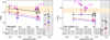 |
Fig. 1 Magnesium abundances for HD 84937 (left) and HD 140283 (right) based on line-by-line equivalent widths. Error bars reflect uncertainties in Teff, log g, [Fe/H], and the ξ adopted in the 1D analysis, as well as a 5% uncertainty in the equivalent width (10% uncertainty for the weak Mg I 473.0 nm line in HD 84937 and for the blended Mg II 448.1 nm line). Weighted lines of best fit for Mg I are shown, excluding the saturated 517 nm triplet and the 457.1 nm line that forms in the upper layers of the photosphere. The shaded horizontal area represents the 3D non-LTE result and its uncertainty from the Mg II 448.1 nm line. The weighted mean abundances, the abundance difference, and their uncertainties indicated in the legend were calculated using the framework from Ji et al. (2020). |
4 Magnesium abundances of stellar populations
In this study, we investigate the possible impact of 3D non-LTE magnesium abundances on stellar populations in the Milky Way using the sample of halo stars from Nissen & Schuster (2010) and the sample of thin-disc stars analysed in Carlos et al. (in prep.)3. All the stars studied in the current work have Teff and ξ from Nissen et al. (2014), while [Fe/H] values were determined by Amarsi et al. (2019). log g for halo stars were also obtained from Nissen et al. (2014), with new log g calculated based on Gaia-DR3 data (Babusiaux et al. 2023; Gaia Collaboration 2023) for the thin-disc sample.The present analysis is based on ID non-LTE and 3D non-LTE solar-differential corrections to the ID LTE [Mg/H] from the abovementioned papers, considering the Mg I 571.1 nm line alone.
Figure 2 shows the results of our re-analysis. As expected, the differential corrections to the solar-normalised [Mg/Fe] are more pronounced at lower metallicities, as these stars are all dwarfs with effective temperatures within several hundred kelvin of the Sun’s. We therefore focussed on halo stars. The original analysis by Nissen & Schuster (2010) identified two distinct stellar populations among halo stars based on precise magnesium abundance with a typical uncertainty of 0.03–0.04 dex, derived from careful analysis of high-resolution, high-S/N spectra. While their analysis was conducted in ID LTE, our 3D non-LTE corrections allow us to explore stellar populations in this sample with more accurate and precise magnesium abundances. This will enable us to investigate if there are further sub-populations, particularly among the α-poor, accreted population, as it is known that more than one galaxy has merged with the Milky Way. The population shows a greater scatter in elemental abundance ratios (Nissen & Schuster 2011), and kinematically selected subsets seem to have slightly different abundance ratios compared to the rest of the α-poor population (see Figs. 5–9 of Matsuno et al. 2022b).
As we transition from ID LTE to ID non-LTE and 3D non-LTE analysis results, a new separation at the metal-rich end (−1 < [Fe/H]) of the α-poor population emerges, while the overall separation between α-rich and a-poor populations is still evident. Figure 3 shows the separations between the α-rich and the two α-poor populations at −1 < [Fe/H]. Additional evidence for the existence of these three distinct populations is provided in Appendix A. The clearer separation between the two α-poor sub-populations is mainly due to the reduced [Mg/Fe] dispersion within each sub-population; the differences in average [Mg/Fe] ratios are 0.10, 0.11, and 0.14 dex in ID LTE, ID non-LTE, and 3D non-LTE, respectively. The scatters are reduced from 0.034 dex to 0.028 and 0.030 dex for the higher [Mg/Fe] α-poor population (α-poor 1) and from 0.033 dex to 0.014 and 0.011 dex for the lower [Mg/Fe] α-poor population (α-poor 2). This suggests that the precision was limited by the approximations of ID and LTE before, and that 3D non-LTE analysis can fully utilise the high S/N ratio of the spectra. Even within the narrow range of stellar parameters in the sample from Nissen & Schuster (2010; 5297 K < Teff < 6445 K and 3.77 < log g < 4.63), the ID non-LTE-lD LTE correction varies from −0.01 to 0.06, with a dispersion of 0.02 dex, and 3D non-LTE–lD non-LTE correction ranges from −0.06 to 0.03 with a similar dispersion. Overall, 3D non-LTE–lD LTE corrections vary from −0.06 to 0.08 with a dispersion of 0.04 dex, which is comparable to or slightly larger than the reported uncertainty on [Mg/Fe] Nissen & Schuster (2010).
Interestingly, the α-poor 1 and 2 populations also differ in kinematics (Fig. 4). The α-poor 1 population stars are preferentially more tightly bound to the Milky Way with low orbital energy, averaging (scatter) 〈E〉 = (−1.77 ± 0.04) × 10s km2 s−2, while the α-poor 2 population stars tend to have high orbital energy with 〈E〉 = (−1.39 + 0.19) × 10s km2 s−2. The kinematics of the α-poor 2 population are consistent with being part of Gaia-Enceladus, suggesting that they trace the chemical evolution of the progenitor galaxy of Gaia-Enceladus. The α-poor 1 population partially overlaps in kinematics with L-RL3.
However, Ruiz-Lara et al. (2022) and Dodd et al. (2023) found its chemistry to be a mixture of hot thick-disc and Gaia-Enceladus, which is not consistent with the chemical properties of our α-poor 1 population. A similar separation was noted in Nissen et al. (2024), which also showed differences in [Na/Fe] (see also Appendix A).
There are outlying populations that deviate from the above overall interpretations and additional stars at lower metallic-ity with [Fe/H] < −1 that require discussion. While G56-30 is chemically classified as an α-poor 2 population with [Fe/H] = −0.88 and [Mg/Fe]3DNLTE = 0.05, it has a low orbital energy (E = −1.79 × 10⁵ km2 s−2), comparable to the α-poor 1 population and the [Na/Fe] ratio between the two populations. Further study with a larger sample with precise and accurate chemical abundance is required to see if there are stars similar to G56-30 and if they can be considered part of Gaia-Enceladus. Another group of stars comprises HD 163810, G176-53, HD 193901, and G21-22, which have [Fe/H] < −1 and seem to have lower [Mg/Fe] than the other stars at the same metallicity. These stars are indicated with open orange squares in Figs. 2 and 4. They stand out less in other elemental abundance ratios, including [Na/Fe], and their kinematics are similar to other α-poor stars, aligning with the distribution of Gaia-Enceladus. Thus, we consider these four stars to be part of Gaia-Enceladus, pending future studies with larger samples.
We further discuss connections of the α-poor 1 population to previously identified stellar populations. While Nissen et al. (2024) initially associated this population with Thamnos, we find this is unlikely due to the small kinematic overlap (Fig. 4). Among the stellar halo populations reported to have intermediate [Mg/Fe] ratios at −1 < [Fe/H], the stellar population named Eos (Myeong et al. 2022) most closely resembles the α-poor 1 population in chemical abundance and kinematics. They identified Eos using a Gaussian mixture model (GMM) analysis of multi-dimensional chemodynamical spaces of giants with high eccentricity in APOGEE DR17 and GALAH DR3, Eos’s existence is confirmed by a t-distributed stochastic neighbor embedding (t-SNE) analysis of halo stars with high-quality spectra in APOGEE (Ortigoza-Urdaneta et al. 2023). The average orbital energy of Eos stars is lower than that of Gaia-Enceladus, resembling our α-poor 1 population in terms of properties (Fig. 4). We therefore consider our α-poor 1 population to be associated with Eos. The sodium abundance of this population also supports its association with Eos (see Nissen et al. 2024).
However, we note that the kinematics of our α-poor 1 population and Eos members from Myeong et al. (2022) are slightly different (Fig. 4). The kinematic pre-selection of stars in Myeong et al. (2022) based on eccentricity excluded stars with high angular momenta, which explains the absence of Eos members in retrograde orbits. Some Eos members have very high orbital energy, which may reflect the overlap between Gaia-Enceladus and Eos in the chemical space. Myeong et al. (2022) also include orbital energy as one of the dimensions in the GMM analyses, which, by design, results in Eos members displaying a single peak in the orbital energy distribution.
Myeong et al. (2022) suggest that Eos formed in situ after the last major merger, likely the accretion of Gaia-Enceladus. Since our sample mostly consists of main-sequence and turn-off stars, rather than APOGEE giants as in Myeong et al. (2022), our stars provide an independent test of the scenario. Using the ages derived by Schuster et al. (2012), we obtained the weighted average age of 10.4 ± 0.4 Gyr (seven stars) for the α-poor 1 population (Eos) and 10.9 ± 0.8 Gyr (three stars) for the α-poor 2 population (Gaia-Enceladus). Hence, there is no significant age difference given the current sample size and measurement uncertainty. If Eos formed shortly after star formation ceased in the progenitor of Gaia-Enceladus, this result aligns with the scenario presented by Myeong et al. (2022).
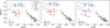 |
Fig. 2 Magnesium abundances for the samples of Nissen & Schuster (2010) and Carlos et al. (in prep.) in ID LTE, ID non-LTE, and 3D non-LTE. In all panels, the Fe abundance is based on a 3D LTE analysis of Fe II lines (Amarsi et al. 2019). The metal-rich end (−1 < [Fe/H]) of the α-poor population is further divided into two, α-poor 1 and 2, based on 3D non-LTE [Mg/Fe] ratios. Four metal-poor α-poor stars are marked with open squares, as they have slightly lower [Mg/Fe] in 3D non-LTE than the other α-poor stars at the same metallicity. |
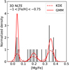 |
Fig. 3 The [Mg/Fe] distribution of metal-rich halo stars with −1 < [Fe/H], The red solid line shows the estimated density based on a Gaussian mixture model (GMM) with three components, while the dashed line shows the density based on a Gaussian kernel density estimation (KDE) with bandwidths of 0.03 dex. Three peaks, corresponding to the α-rich population and the two α-poor sub-populations, are clearly visible in both density estimations. |
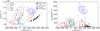 |
Fig. 4 Kinematics of sub-populations. Angular momentum and orbital energy were computed in the same manner as in Matsuno et al. (2022b), with Lperp defined as |

5 Conclusion
In this study, we constructed a grid of abundance corrections required to adjust 1D LTE magnesium abundances with the 3D non-LTE scale for main-sequence turn-off stars with 5000 K ≲ Teff ≲ 6500 K, log g = 4.0 and 4.5, −3.0 ≤ [Fe/H] ≤ 0.0, and 1D LTE ξ of 0, 1, and 2 km s−1. The impact of the 3D non-LTE corrections was demonstrated on the benchmark metal-poor stars HD 84937 and HD 140283, and shown to significantly reduce the large ionisation imbalances found in both 1D LTE and 1D non-LTE.
Further demonstrating the impact of 3D non-LTE corrections in the context of galactic archaeology, we applied these to a sample of halo stars from Nissen & Schuster (2010). Their α-poor population, previously interpreted as an accreted population, exhibits (at least) two distinct sub-populations in 3D non-LTE magnesium abundance. While the two sub-populations show different average magnesium abundances in 1D LTE or 1D non-LTE, a clear separation can be observed for the first time in 3D non-LTE thanks to the increased precision. Although the sample was selected to have a narrow range in stellar parameters, the correction from 1D LTE to 3D non-LTE in [Mg/Fe] varies from −0.06 dex to +0.08 dex with a dispersion of 0.04 dex. Thus, the 1D LTE approximations can limit achieving high precision when high-quality spectra with R > 50 000 and S/N > 100 similar to those used by Nissen & Schuster (2010) are available.
The two α-poor sub-populations also differ in kinematics. The sub-population with the lower [Mg/Fe] shows highly radial orbits, consistent with being part of Gaia-Enceladus, while the other sub-population is more tightly bound to the Milky Way’s gravitational potential. The [Mg/Fe] and kinematics, as well as the [Na/Fe] (Nissen et al. 2024) of the latter population, resemble those of the stellar population dubbed Eos (Myeong et al. 2022). Although Eos was identified using a GMM analysis in a chemodynamical space of stars with highly eccentric orbits, we show that Gaia-Enceladus and Eos members can be cleanly selected without kinematic preselection with precise and accurate 3D non-LTE magnesium abundances. Applying such selections to a larger sample will enable the study of their intrinsic distributions in age, present-day kinematics, and other elemental abundance ratios, revealing the formation histories of stellar populations in the Milky Way.
Acknowledgements
We thank the anonymous referee for their helpful and constructive comments. We thank Per Jönsson and Henrik Hartman (Malmö Uni-versitet) for useful discussions about the Mg I oscillator strengths. We also thank Gyuchul Myeong for sharing the lists of Eos member stars with us. T.M. was supported by a Spinoza Grant from the Dutch Research Council (NWO), which was awarded to Prof. Amina Helmi, and by a Gliese Fellowship at the Zentrum für Astronomie, University of Heidelberg, Germany. AMA acknowledges support from the Swedish Research Council (VR 2020-03940). This research was supported by computational resources provided by the Australian Government through the National Computational Infrastructure (NCI) under the National Computational Merit Allocation Scheme and the ANU Merit Allocation Scheme (project y89). Some of the computations were also enabled by resources provided by the Swedish National Infrastructure for Computing (SNIC) at the Multi-disciplinary Center for Advanced Computational Science (UPPMAX) partially funded by the Swedish Research Council through grant agreement no. 201805973. MC acknowledges the support from the Knut and Alice Wallenberg Foundation as part of the project “Probing charge- and mass-transfer reactions on the atomic level” (2018.0028).
Appendix A: Further evidence for the three distinct populations
This section provides a statistical confirmation of the presence of the two α-poor sub-populations and the separation between the α-rich and a-poor populations among halo stars at −1 < [Fe/H]. As shown in Fig. 3, the [Mg/Fe] ratio distribution among the metal-rich halo stars is best fitted with three components when GMMs are used. We evaluated each GMM with a different number of components using the Bayesian information criterion (BIC), which is summarized in Table A.1. The GMM with three components is most favoured according to the BIC. Notably, the BiC difference between the GMMs with two and three components is more than six, which is interpreted as a strong preference for the three-component model. The three components correspond to the high-α, α-poor 1 and 2 populations.
We have shown in the main text that the separation between α-poor 1 and 2 populations is also seen in kinematics. As indicated by Nissen et al. (2024), the two populations also differ in other elemental abundances, such as [Na/Fe], which is shown in Fig. A.1. This reinforces our finding that α-poor 1 and 2 populations have astrophysically different origins.
BIC of GMMs
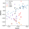 |
Fig. A.1 [Na/Fe] ratios of halo stars. The non-LTE Na abundances are taken from Nissen et al. (2024). |
References
- Abdurro’uf, Accetta, K., Aerts, C., et al. 2022, ApJS, 259, 35 [NASA ADS] [CrossRef] [Google Scholar]
- Alexeeva, S., Ryabchikova, T., Mashonkina, L., & Hu, S. 2018, ApJ, 866, 153 [Google Scholar]
- Altrock, R. C., & Cannon, C. J. 1975, Sol. Phys., 42, 289 [NASA ADS] [CrossRef] [Google Scholar]
- Amarsi, A. M., Lind, K., Asplund, M., Barklem, P. S., & Collet, R. 2016, MNRAS, 463, 1518 [NASA ADS] [CrossRef] [Google Scholar]
- Amarsi, A. M., Nordlander, T., Barklem, P. S., et al. 2018, A&A, 615, A139 [NASA ADS] [CrossRef] [EDP Sciences] [Google Scholar]
- Amarsi, A. M., Nissen, P. E., & Skúladóttir, Á. 2019, A&A, 630, A104 [NASA ADS] [CrossRef] [EDP Sciences] [Google Scholar]
- Amarsi, A. M., Lind, K., Osorio, Y., et al. 2020, A&A, 642, A62 [EDP Sciences] [Google Scholar]
- Amarsi, A. M., Liljegren, S., & Nissen, P. E. 2022, A&A, 668, A68 [NASA ADS] [CrossRef] [EDP Sciences] [Google Scholar]
- Asplund, M., Grevesse, N., Sauval, A. J., & Scott, P. 2009, ARA&A, 47, 481 [NASA ADS] [CrossRef] [Google Scholar]
- Asplund, M., Amarsi, A. M., & Grevesse, N. 2021, A&A, 653, A141 [NASA ADS] [CrossRef] [EDP Sciences] [Google Scholar]
- Babusiaux, C., Fabricius, C., Khanna, S., et al. 2023, A&A, 674, A32 [NASA ADS] [CrossRef] [EDP Sciences] [Google Scholar]
- Barklem, P. S. 2016a, A&A Rev., 24, 9 [NASA ADS] [CrossRef] [Google Scholar]
- Barklem, P. S. 2016b, Phys. Rev. A, 93, 042705 [NASA ADS] [CrossRef] [Google Scholar]
- Belyaev, A. K., & Yakovleva, S. A. 2017, A&A, 606, A147 [NASA ADS] [CrossRef] [EDP Sciences] [Google Scholar]
- Belokurov, V., Erkal, D., Evans, N. W., Koposov, S. E., & Deason, A. J. 2018, MNRAS, 478, 611 [Google Scholar]
- Bergemann, M., Collet, R., Amarsi, A. M., et al. 2017, ApJ, 847, 15 [NASA ADS] [CrossRef] [Google Scholar]
- Buder, S., Sharma, S., Kos, J., et al. 2021, MNRAS, 506, 150 [NASA ADS] [CrossRef] [Google Scholar]
- Casagrande, L., Ramírez, I., Meléndez, J., Bessell, M., & Asplund, M. 2010, A&A, 512, A54 [NASA ADS] [CrossRef] [EDP Sciences] [Google Scholar]
- Chang, T. N., & Tang, X. 1990, J. Quant. Spec. Radiat. Transf., 43, 207 [NASA ADS] [CrossRef] [Google Scholar]
- Dodd, E., Callingham, T. M., Helmi, A., et al. 2023, A&A, 670, L2 [NASA ADS] [CrossRef] [EDP Sciences] [Google Scholar]
- Froese Fischer, C., Tachiev, G., & Irimia, A. 2006, At. Data Nucl. Data Tables, 92, 607 [NASA ADS] [CrossRef] [Google Scholar]
- Fuhrmann, K. 1998, A&A, 338, 161 [NASA ADS] [Google Scholar]
- Gaia Collaboration (Vallenari, A., et al.) 2023, A&A, 674, A1 [NASA ADS] [CrossRef] [EDP Sciences] [Google Scholar]
- Giribaldi, R. E., da Silva, A. R., Smiljanic, R., & Cornejo Espinoza, D. 2021, A&A, 650, A194 [NASA ADS] [CrossRef] [EDP Sciences] [Google Scholar]
- Godone, A., & Novero, C. 1992, Phys. Rev. A, 45, 1717 [NASA ADS] [CrossRef] [Google Scholar]
- Grevesse, N., Asplund, M., & Sauval, A. J. 2007, The Solar Chemical Composition, eds. R. von Steiger, G. Gloeckler, & G. M. Mason (Springer Science+Business Media), 105 [Google Scholar]
- Gustafsson, B., Edvardsson, B., Eriksson, K., et al. 2008, A&A, 486, 951 [NASA ADS] [CrossRef] [EDP Sciences] [Google Scholar]
- Heiter, U., Jofré, P., Gustafsson, B., et al. 2015, A&A, 582, A49 [NASA ADS] [CrossRef] [EDP Sciences] [Google Scholar]
- Helmi, A., Babusiaux, C., Koppelman, H. H., et al. 2018, Nature, 563, 85 [Google Scholar]
- Horta, D., Schiavon, R. P., Mackereth, J. T., et al. 2023, MNRAS, 520, 5671 [NASA ADS] [CrossRef] [Google Scholar]
- Ji, A. P., Li, T. S., Hansen, T. T., et al. 2020, AJ, 160, 181 [NASA ADS] [CrossRef] [Google Scholar]
- Jofré, P., Heiter, U., Soubiran, C., et al. 2015, A&A, 582, A81 [Google Scholar]
- Jönsson, P., & Froese Fischer, C. 1997, in APS April Meeting Abstracts, J15.37 [Google Scholar]
- Karovicova, I., White, T. R., Nordlander, T., et al. 2018, MNRAS, 475, L81 [Google Scholar]
- Karovicova, I., White, T. R., Nordlander, T., et al. 2020, A&A, 640, A25 [NASA ADS] [CrossRef] [EDP Sciences] [Google Scholar]
- Lagae, C., Amarsi, A. M., Rodríguez Díaz, L. F., et al. 2023, A&A, 672, A90 [NASA ADS] [CrossRef] [EDP Sciences] [Google Scholar]
- Lambert, D. L. 1993, Physica Scripta Volume T, 47, 186 [NASA ADS] [CrossRef] [Google Scholar]
- Langangen, Ø., & Carlsson, M. 2009, ApJ, 696, 1892 [NASA ADS] [CrossRef] [Google Scholar]
- Lawler, J. E., Guzman, A., Wood, M. P., Sneden, C., & Cowan, J. J. 2013, ApJS, 205, 11 [Google Scholar]
- Leenaarts, J., & Carlsson, M. 2009, in The Second Hinode Science Meeting, eds. B. Lites, M. Cheung, T. Magara, J. Mariska, & K. Reeves, ASP, 415, 87 [NASA ADS] [Google Scholar]
- Lind, K., Nordlander, T., Wehrhahn, A., et al. 2022, A&A, 665, A33 [NASA ADS] [CrossRef] [EDP Sciences] [Google Scholar]
- Magic, Z., Collet, R., Asplund, M., et al. 2013, A&A, 557, A26 [NASA ADS] [CrossRef] [EDP Sciences] [Google Scholar]
- Mallinson, J. W. E., Lind, K., Amarsi, A. M., et al. 2022, A&A, 668, A103 [NASA ADS] [CrossRef] [EDP Sciences] [Google Scholar]
- Mallinson, J. W. E., Lind, K., Amarsi, A. M., & Youakim, K. 2024, A&A, 687, A5 [NASA ADS] [CrossRef] [EDP Sciences] [Google Scholar]
- Matsuno, T., Dodd, E., Koppelman, H. H., et al. 2022a, A&A, 665, A46 [NASA ADS] [CrossRef] [EDP Sciences] [Google Scholar]
- Matsuno, T., Koppelman, H. H., Helmi, A., et al. 2022b, A&A, 661, A103 [NASA ADS] [CrossRef] [EDP Sciences] [Google Scholar]
- Myeong, G. C., Belokurov, V., Aguado, D. S., et al. 2022, ApJ, 938, 21 [NASA ADS] [CrossRef] [Google Scholar]
- Nissen, P. E., & Schuster, W. J. 2010, A&A, 511, L10 [NASA ADS] [CrossRef] [EDP Sciences] [Google Scholar]
- Nissen, P. E., & Schuster, W. J. 2011, A&A, 530, A15 [NASA ADS] [CrossRef] [EDP Sciences] [Google Scholar]
- Nissen, P. E., Chen, Y. Q., Carigi, L., Schuster, W. J., & Zhao, G. 2014, A&A, 568, A25 [NASA ADS] [CrossRef] [EDP Sciences] [Google Scholar]
- Nissen, P. E., Amarsi, A. M., Skúladóttir, Á., & Schuster, W. J. 2024, A&A, 682, A116 [NASA ADS] [CrossRef] [EDP Sciences] [Google Scholar]
- Ortigoza-Urdaneta, M., Vieira, K., Fernández-Trincado, J. G., et al. 2023, A&A, 676, A140 [NASA ADS] [CrossRef] [EDP Sciences] [Google Scholar]
- Osorio, Y., Barklem, P. S., Lind, K., et al. 2015, A&A, 579, A53 [NASA ADS] [CrossRef] [EDP Sciences] [Google Scholar]
- Pehlivan Rhodin, A., Hartman, H., Nilsson, H., & Jönsson, P. 2017, A&A, 598, A102 [NASA ADS] [CrossRef] [EDP Sciences] [Google Scholar]
- Ralchenko, Y., & Kramida, A. 2020, Atoms, 8, 56 [NASA ADS] [CrossRef] [Google Scholar]
- Ruiz-Lara, T., Matsuno, T., Lövdal, S. S., et al. 2022, A&A, 665, A58 [NASA ADS] [CrossRef] [EDP Sciences] [Google Scholar]
- Schuster, W. J., Moreno, E., Nissen, P. E., & Pichardo, B. 2012, A&A, 538, A21 [NASA ADS] [CrossRef] [EDP Sciences] [Google Scholar]
- Weinberg, D. H., Holtzman, J. A., Hasselquist, S., et al. 2019, ApJ, 874, 102 [NASA ADS] [CrossRef] [Google Scholar]
- Zhou, Y., Amarsi, A. M., Aguirre Børsen-Koch, V., et al. 2023, A&A, 677, A98 [NASA ADS] [CrossRef] [EDP Sciences] [Google Scholar]
 .
.
As shown in their Table 6, labelled Δfgh.
We note that an earlier version of our 3D non-LTE corrections was applied to the sample of Nissen & Schuster (2010) in Nissen et al. (2024).
All Tables
Equivalent widths W, reduced equivalent widths REW = log(W/λvac), 3D non-LTE abundance, and abundance corrections in HD 84937 and HD 140283.
All Figures
|
Fig. 1 Magnesium abundances for HD 84937 (left) and HD 140283 (right) based on line-by-line equivalent widths. Error bars reflect uncertainties in Teff, log g, [Fe/H], and the ξ adopted in the 1D analysis, as well as a 5% uncertainty in the equivalent width (10% uncertainty for the weak Mg I 473.0 nm line in HD 84937 and for the blended Mg II 448.1 nm line). Weighted lines of best fit for Mg I are shown, excluding the saturated 517 nm triplet and the 457.1 nm line that forms in the upper layers of the photosphere. The shaded horizontal area represents the 3D non-LTE result and its uncertainty from the Mg II 448.1 nm line. The weighted mean abundances, the abundance difference, and their uncertainties indicated in the legend were calculated using the framework from Ji et al. (2020). |
| In the text | |
|
Fig. 2 Magnesium abundances for the samples of Nissen & Schuster (2010) and Carlos et al. (in prep.) in ID LTE, ID non-LTE, and 3D non-LTE. In all panels, the Fe abundance is based on a 3D LTE analysis of Fe II lines (Amarsi et al. 2019). The metal-rich end (−1 < [Fe/H]) of the α-poor population is further divided into two, α-poor 1 and 2, based on 3D non-LTE [Mg/Fe] ratios. Four metal-poor α-poor stars are marked with open squares, as they have slightly lower [Mg/Fe] in 3D non-LTE than the other α-poor stars at the same metallicity. |
| In the text | |
|
Fig. 3 The [Mg/Fe] distribution of metal-rich halo stars with −1 < [Fe/H], The red solid line shows the estimated density based on a Gaussian mixture model (GMM) with three components, while the dashed line shows the density based on a Gaussian kernel density estimation (KDE) with bandwidths of 0.03 dex. Three peaks, corresponding to the α-rich population and the two α-poor sub-populations, are clearly visible in both density estimations. |
| In the text | |
|
Fig. 4 Kinematics of sub-populations. Angular momentum and orbital energy were computed in the same manner as in Matsuno et al. (2022b), with Lperp defined as |
| In the text | |
|
Fig. A.1 [Na/Fe] ratios of halo stars. The non-LTE Na abundances are taken from Nissen et al. (2024). |
| In the text | |
Current usage metrics show cumulative count of Article Views (full-text article views including HTML views, PDF and ePub downloads, according to the available data) and Abstracts Views on Vision4Press platform.
Data correspond to usage on the plateform after 2015. The current usage metrics is available 48-96 hours after online publication and is updated daily on week days.
Initial download of the metrics may take a while.