| Issue |
A&A
Volume 693, January 2025
|
|
|---|---|---|
| Article Number | A76 | |
| Number of page(s) | 15 | |
| Section | Interstellar and circumstellar matter | |
| DOI | https://doi.org/10.1051/0004-6361/202452686 | |
| Published online | 03 January 2025 | |
Dissecting the disk and the jet of a massive (proto)star
An ALMA view of IRAS 20126+4104
1
INAF, Osservatorio Astrofisico di Arcetri,
Largo E. Fermi 5,
50125
Firenze,
Italy
2
Centro de Astrobiología (CAB), CSIC-INTA,
Carretera de Ajalvir km 4, Torrejón de Ardoz,
28850
Madrid,
Spain
3
Institut de Ciències de l’Espai (ICE, CSIS), Carrer de Can Magrans s/n,
08193
Bellaterra,
Spain
4
Institut d’Estudis Espacials de Catalunya (IEEC),
Barcelona,
Spain
★ Corresponding author; This email address is being protected from spambots. You need JavaScript enabled to view it.
Received:
21
October
2024
Accepted:
2
December
2024
Abstract
Context. The study of disks around early-type (proto)stars has recently been boosted by a new generation of instruments, and additional evidence has been found of disk+jet systems around stars of up to ~20 M⊙. These results appear to confirm theoretical predictions that even the most massive stars may form though disk-mediated accretion.
Aims. We want to investigate one of the best examples of disk+jet systems around an early B-type (proto)star, IRAS 20126+4104. The relatively simple structure of this object and its relative proximity to Earth (1.64 kpc) make it an ideal target for resolution of its disk and the determination of its physical and kinematical structure.
Methods. Despite the high declination of IRAS 20126+4104, it has been possible to perform successful observations with the Atacama Large Millimeter and submillimeter Array at 1.4 mm in the continuum emission and a number of molecular tracers of high-density gas (for the disk) and shocked gas (for the jet).
Results. The new data allow us to improve on previous similar observations of IRAS 20126+4104 and confirm the existence of a Keplerian accretion disk around a ~12 M⊙ (proto)star. From methyl cyanide, we derived the rotation temperature and column density as a function of disk radius. We also obtained a map of the same quantities for the jet using the ratio between two lines of formaldehyde. We also use two simple models of the jet and the disk to estimate the basic geometrical and kinematical parameters of the two. From the temperature and column density profiles, we conclude that the disk is stable at all radii. We also estimate an accretion rate of ~10−3 M⊙ yr−1.
Conclusions. Our analysis confirms that the jet from IRAS 20126+4104 is highly collimated, lies close to the plane of the sky, and expands with velocity increasing with distance. As expected, the gas temperature and column density peak in the bow shock. The disk is undergoing Keplerian rotation but a non-negligible radial velocity component is also present that is equal to ~40% of the rotational component. The disk is slightly inclined with respect to the line of sight and has a dusty envelope that absorbs the emission from the disk surface. This causes a slight distortion of the disk structure observed in high-density tracers such as methyl cyanide. We also reveal a significant deviation from axial symmetry in the SW part of the disk, which might be caused by either tidal interaction with a nearby, lower-mass companion or interaction with the outflowing gas of the jet.
Key words: accretion, accretion disks / stars: formation / stars: massive / ISM: jets and outflows
© The Authors 2025
 Open Access article, published by EDP Sciences, under the terms of the Creative Commons Attribution License (https://creativecommons.org/licenses/by/4.0), which permits unrestricted use, distribution, and reproduction in any medium, provided the original work is properly cited.
This article is published in open access under the Subscribe to Open model. This email address is being protected from spambots. You need JavaScript enabled to view it. to support open access publication.
1 Introduction
The important role played by disks in the process of star formation is amply evidenced by the plenitude of proto-planetary disks found around Solar-type (proto)stars in recent years (e.g., Benisty et al. 2023). The impressive images obtained with the Atacama Large Millimeter and submillimeter Array (ALMA) have allowed extremely detailed studies of the disk structure and have revealed the presence of a variety of structures from gaps to spiral arms (e.g., Garufi et al. 2018; Andrews 2020). The situation is quite different for early-type, and especially O-type, (proto)stars. While ALMA observations have increased the number of candidate circumstellar disks around massive (proto)stars, none of these resemble the disks around their low-mass siblings. A reason for this difference is certainly the large distances to these objects (typically a few kiloparsecs), which imply linear resolutions of >100 au. Another reason is that high-mass stars are born deeply embedded in their parental, optically thick cores, which makes it difficult to distinguish the disk from the envelope enshrouding it. In addition, the presence of rich stellar clusters, besides complicating the observations, may also affect the disk structure by tidal interactions, thus altering the disk morphology and velocity field; and multiple (proto)stars power multiple outflows, which makes the picture even more confused.
For these reasons, we must focus on the most promising disk candidates around massive stars, as this strategy allows us to obtain the greatest amount of information on these objects through high-resolution observations. One of the first and best studied disk+jet systems associated with a massive young stellar object (YSO) is certainly IRAS 20126+4104. This object has been observed in a large number of tracers over a broad range of wavelengths, spanning from the centimeter regime to X-rays. Here, we summarize the main findings from the literature that are the most relevant to the present study and explain why we decided to focus our attention on IRAS 20126+4104 in particular.
The distance estimate, obtained from parallax measurements of the H2O masers, ranges from ![Mathematical equation: $\[1.33_{-0.15}^{+0.19}\]$](/articles/aa/full_html/2025/01/aa52686-24/aa52686-24-eq1.png) (Hirota et al. 2020) to 1.64±0.05 kpc (Moscadelli et al. 2011), which are consistent with each other to within 1.3 σ. In the following, we adopt a distance of 1.64 kpc because of the smaller error and for consistency with previous studies of IRAS 20126+4104. The source appears to be relatively isolated in the near-infrared (Qiu et al. 2008), but X-ray observations have revealed a deeply embedded cluster associated with it (Montes et al. 2015). The main feature of IRAS 20126+4104 is the presence of a circumstellar structure, which appears to undergo Keplerian rotation around a (proto)star of ~104 L⊙ (Cesaroni et al. 1997, 1999, 2023). Model fits to the spectral energy distribution as well as to the molecular line data have been performed by several authors (Keto & Zhang 2010; Johnston et al. 2011; Chen et al. 2016), who derive a stellar mass of ~12 M⊙. The lack of a detectable H II region around such a massive and luminous star suggests that accretion might still be present, quenching the formation of such a region (see Walmsley 1995). The object is also powering a thermal radio jet (Hofner et al. 1999, 2007), and exhibits a molecular outflow (Wilking et al. 1990; Cesaroni et al. 1997, 1999; Kawamura et al. 1999) that is roughly perpendicular to the disk and is undergoing precession, probably due to a nearby star (Shepherd et al. 2000; Cesaroni et al. 2005; Caratti o Garatti et al. 2008). The expansion of the jet has been measured by means of the H2O maser proper motions down to ~100 au from the star (Moscadelli et al. 2005, 2011) and with multi-epoch imaging of the H2 jet up to ~104 au (Massi et al. 2023).
(Hirota et al. 2020) to 1.64±0.05 kpc (Moscadelli et al. 2011), which are consistent with each other to within 1.3 σ. In the following, we adopt a distance of 1.64 kpc because of the smaller error and for consistency with previous studies of IRAS 20126+4104. The source appears to be relatively isolated in the near-infrared (Qiu et al. 2008), but X-ray observations have revealed a deeply embedded cluster associated with it (Montes et al. 2015). The main feature of IRAS 20126+4104 is the presence of a circumstellar structure, which appears to undergo Keplerian rotation around a (proto)star of ~104 L⊙ (Cesaroni et al. 1997, 1999, 2023). Model fits to the spectral energy distribution as well as to the molecular line data have been performed by several authors (Keto & Zhang 2010; Johnston et al. 2011; Chen et al. 2016), who derive a stellar mass of ~12 M⊙. The lack of a detectable H II region around such a massive and luminous star suggests that accretion might still be present, quenching the formation of such a region (see Walmsley 1995). The object is also powering a thermal radio jet (Hofner et al. 1999, 2007), and exhibits a molecular outflow (Wilking et al. 1990; Cesaroni et al. 1997, 1999; Kawamura et al. 1999) that is roughly perpendicular to the disk and is undergoing precession, probably due to a nearby star (Shepherd et al. 2000; Cesaroni et al. 2005; Caratti o Garatti et al. 2008). The expansion of the jet has been measured by means of the H2O maser proper motions down to ~100 au from the star (Moscadelli et al. 2005, 2011) and with multi-epoch imaging of the H2 jet up to ~104 au (Massi et al. 2023).
Given the relative proximity and simple structure of the source, which make IRAS 20126+4104 an ideal disk+jet system for study, we decided to use the most powerful millimeter interferometer available to date in order to analyze the structure and kinematics of this object. Despite the high declination of the source, the observations are feasible with ALMA, and the new data are an improvement by at least a factor of ~2 in angular resolution and ~5 in sensitivity with respect to previous observations at the same wavelengths (Cesaroni et al. 1999, 2014; Su et al. 2011).
2 Observations and data reduction
The ALMA observations of IRAS 20126+4104 were performed in band 6 at three epochs, on May 20, 2017, July 6, 2017, and October 25, 2021 (projects 2016.1.00595.S and 2019.1.00199.S). The phase center of the observations was ![Mathematical equation: $\[\alpha(\text{ICRS}){=}20^{\mathrm{h}} 14^{\mathrm{m}} 26^{\mathrm{s}}_\cdot0364\]$](/articles/aa/full_html/2025/01/aa52686-24/aa52686-24-eq2.png) and
and ![Mathematical equation: $\[\delta(\text{ICRS}){=}41^{\circ} 13^{\prime} 32^{\prime \prime}_\cdot516\]$](/articles/aa/full_html/2025/01/aa52686-24/aa52686-24-eq3.png) . For the observations made in 2017, J2025+3343 and J2148+0657 were used as bandpass and flux calibrator, respectively, whereas in 2021, J2253+1608 was used for both calibrations. In all cases, the phase calibrator was J2015+3710. The correlator configuration consisted of one unit of 1.875 GHz and 12 units of 234 MHz.
. For the observations made in 2017, J2025+3343 and J2148+0657 were used as bandpass and flux calibrator, respectively, whereas in 2021, J2253+1608 was used for both calibrations. In all cases, the phase calibrator was J2015+3710. The correlator configuration consisted of one unit of 1.875 GHz and 12 units of 234 MHz.
The data were calibrated with the ALMA data-reduction pipeline and subsequent data flagging and imaging were made with the Common Astronomy Software Applications (CASA) software1. We created cubes with natural weighting covering all of the correlator units, using only the data obtained with the compact configuration in 2017. The data were corrected for primary beam attenuation. The continuum was subtracted with the STATCONT software2 developed by Sánchez-Monge et al. (2018). Then all line cubes were inspected to search for possible outflow tracers besides the J=2−1 transition of the well-known CO isotopologs and the SiO(5–4) line. As a result, we found a further four lines that originate from the outflow lobes, namely the H2CO(30,3–20,2), (32,2–22,1), and (32,1–22,0) transitions and the CH3OH(4−2,3–3−1,2) E line. In practice, only the SiO, H2CO, and CH3OH data were usable for our study, because the 13CO and C18O line emission were heavily resolved out. The synthesized beam of the images is about ![Mathematical equation: $\[0^{\prime\prime}_\cdot48 \times 0^{\prime\prime}_\cdot28\]$](/articles/aa/full_html/2025/01/aa52686-24/aa52686-24-eq4.png) with a position angle (PA) of −7°.
with a position angle (PA) of −7°.
We also created cubes with natural weighting using all the available configurations (i.e., the data from both 2017 and 2021) only for the correlator unit covering the largest bandwidth (1.875 GHz) and those containing selected molecular species that we wish to use for studying the disk, specifically the CH3CN isotopologs and DCN. We then obtained a continuum image from the cube spanning the 1.875 GHz bandwidth with STATCONT, whereas we preferred to subtract the continuum from the other cubes by removing a constant baseline fitted to line-free channels selected by visual inspection of the spectra. The resulting synthesized beam is approximately ![Mathematical equation: $\[0^{\prime\prime}_\cdot23 \times 0^{\prime\prime}_\cdot13\]$](/articles/aa/full_html/2025/01/aa52686-24/aa52686-24-eq5.png) with a PA of −12°. The final images were converted to GILDAS format and analyzed with the GILDAS3 software.
with a PA of −12°. The final images were converted to GILDAS format and analyzed with the GILDAS3 software.
3 Results
Based on previous studies (see, e.g., Cesaroni et al. 1999, 2014 and Su et al. 2011), we know that the disk in IRAS 20126+4104 is best imaged in the millimeter continuum emission and in complex organic molecules (COMs) such as CH3CN, whereas a typical shock tracer observed in the outflowing gas is SiO. For the sake of simplicity, hereafter we refer to the collimated bipolar structure observed in SiO as the “jet”. This structure is also detected in other molecules (see Sect. 3.1) prominent in the disk. In this section, we describe the results obtained for the disk and the jet from the analysis of selected molecular species, namely three CH3CN isotopologs, DCN, CH3OH, H2CO, and SiO.
3.1 The jet
As mentioned in Sect. 1, the jet+outflow from IRAS 20126+4104 has been studied in detail by several authors. Here we take advantage of the high sensitivity of our ALMA observations to perform an improved analysis of the jet structure and physical parameters on scales of up to ~0.06 pc or 12 000 au. For this purpose, we inspected the data cubes covering the whole frequency range of our correlator setup and found five lines belonging to three molecular species that appear to trace the jet, namely the SiO(5–4) (upper level energy Eu=31 K), CH3OH (4−2,3–3−1,2) E (Eu=45 K), and H2CO (30,3–20,2) (Eu=21 K), (32,2–22,1) (Eu=68 K) and (32,1–22,0) (Eu=68 K) transitions. As the latter two transitions have the same excitation energies and line strengths, we decided to average the two data sets to improve the signal-to-noise ratio (S/N). A comparison among the moment-8 maps4 of all these lines and the H2 2.12 μm line imaged by Cesaroni et al. (2013) and Massi et al. (2023) is shown in Fig. 1. We note that, unlike the bow shock to the SE, which is detected only in the SiO line, the one to the NW is traced by all molecules. It is also interesting to note that the emission in different molecules peaks at different places in the NW bow shock. In particular, the H2 emission appears to lie downstream (i.e., closer to the center of ejection) with respect to the SiO shock, whereas both the CH3OH and H2CO emissions are located upstream (i.e., farther from the center of ejection), an effect that can be better appreciated in Fig. 2, where we show the emission in the different tracers along the jet axis passing through the NW lobe. This configuration could mirror a chemical stratification possibly due to temperature and density gradients across the bow shock, although excitation effects due to the variation of these physical parameters cannot be excluded.
The complementary distribution of the different tracers is observed also in the velocity field of the bow shocks, which is revealed by the position-velocity (PV) diagrams in Fig. 3 along the jet axis (i.e., along a cut with PAja≃−60°). These were obtained with the same method used for the moment-8 maps: for each pixel of the PV diagram, we took the maximum emission along the direction perpendicular to the jet axis. Clearly, the CH3OH and H2CO emission covers approximately the same area in the plot, and both are complementary to the SiO emission. We note that the contours of the PV diagrams have been chosen in such a way to emphasise the emission from the lobes, while that from the core is illustrated in Sect. 3.2. However, it is clear that the strongest H2CO and CH3OH emission is seen around the star, unlike the SiO emission, which is dominant at the tips of the jet lobes, as expected for a shock tracer. We analyze the structure of the bow shock in more detail in Sect. 4.1.
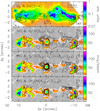 |
Fig. 1 Moment-8 maps in various molecular tracers of the jet in IRAS 20126+4104. All maps have been rotated by 30° clockwise so that the jet axis lies parallel to the X-axis of the plot. The offset is relative to the phase center of the observations. The ellipse in the bottom left corner indicates the synthesized beam of the ALMA maps. (a) Contour map of the SiO(5–4) line emission overlaid on the image of the H2 2.12 μm line obtained by Cesaroni et al. (2013). Contour levels range from 10.4 to 136.4 in steps of 21 mJy/beam. (b) Contour map of the H2CO (30,3–20,2) line emission overlaid on the same SiO(5–4) image as in panel a. Contour levels range from 27 to 117 in steps of 15 mJy/beam. (c) Same as panel b but for the contour map of the average emission in the H2CO (32,2–22,1) and (32,1–22,0) lines. Contour levels range from 12 to 111 in steps of 9 mJy/beam. (d) Same as panel b but for the contour map of the CH3OH (4−2,3–3−1,2) E line emission. Contour levels range from 16.2 to 111.2 in steps of 19 mJy/beam. |
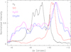 |
Fig. 2 Normalized intensity profile along the jet axis. The X-axis is the same as in Fig. 1 but spans only the range of angles corresponding to the NW lobe of the jet. The meaning of the different curves is given in the figure. |
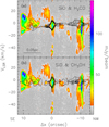 |
Fig. 3 Moment-8 PV diagrams in three molecular tracers of the jet along the direction with a PA of −60°. The offset is relative to the phase center of the observations. The cross in the bottom left corner indicates the angular and spectral resolutions. (a) Contour map of the H2CO (30,3–20,2) line emission overlaid on the SiO(5–4) map. Contour levels range from 22 to 112 in steps of 15 mJy/beam. (b) Same as panel a but for the contour map of the CH3OH (4−2,3–3−1,2) E line emission. Contour levels range from 16.2 to 111.2 in steps of 19 mJy/beam. |
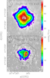 |
Fig. 4 Map of the 1.4 mm continuum emission (contours) overlaid on the moment-8 map of the CH3CN(12–11) K=3 (panel a) and 13CH3CN(13–12) K=3 line (panel b). Contour levels range from 1.4 to 26.6 in steps of 2.8 mJy/beam. The ellipses in the bottom left and right corners indicate the synthesized beam of the continuum and line maps, respectively. |
3.2 The disk
The contour map in Fig. 4 shows that the continuum emission is made of an extended halo with a barely resolved peak of emission at the center, which in the following we assume to pin-point the position of the (proto)star. This morphology suggests that the continuum is arising from both the disk and a surrounding envelope. We fitted the continuum map with a 2D Gaussian using task imfit of CASA. The position of the 1.4 mm continuum peak obtained in this way provides us with an estimate of the disk center (i.e., the position of the star), which is ![Mathematical equation: $\[\alpha(\mathrm{J} 2000){=}20^{\mathrm{h}} 14^{\mathrm{m}} 26^\mathrm{s}_\cdot022 \pm 0^\mathrm{s}_\cdot0011\]$](/articles/aa/full_html/2025/01/aa52686-24/aa52686-24-eq6.png) and
and ![Mathematical equation: $\[\delta(\mathrm{J} 2000){=}41^{\circ} 13^{\prime} 32^{\prime \prime}_\cdot58{\pm}0^{\prime \prime}_\cdot013\]$](/articles/aa/full_html/2025/01/aa52686-24/aa52686-24-eq7.png) . The deconvolved full width at half maximum (FWHM) is
. The deconvolved full width at half maximum (FWHM) is ![Mathematical equation: $\[(\left.0^{\prime\prime}_\cdot 71{\pm}0^{\prime\prime}_\cdot04\right){\times}\left(0^{\prime\prime}_\cdot58{\pm}0^{\prime\prime}_\cdot04\right.)\]$](/articles/aa/full_html/2025/01/aa52686-24/aa52686-24-eq8.png) or (1160±70)×(950±70) au with a PA of 56°±15°. We note that the latter value is consistent within the error with the PA of the major axis of the disk derived by other authors (53°; Cesaroni et al. 2005) from their CH3CN line data.
or (1160±70)×(950±70) au with a PA of 56°±15°. We note that the latter value is consistent within the error with the PA of the major axis of the disk derived by other authors (53°; Cesaroni et al. 2005) from their CH3CN line data.
The emission from the disk is illustrated in Fig. 4 by the moment-8 maps of the CH3CN (12–11) and 13CH3CN(13–12) line emission. We have chosen the K=3 component, which is the least affected by blending with other transitions. As expected, the thinner 13CH3CN line emission is detected over a more compact region than the main species, while the extension of the latter approximately matches that of the continuum emission. Another obvious difference between Figs. 4a and 4b is that in the former the emission is maximum around the continuum peak, whereas in the latter the peak of the emission is clearly shifted to the WSW. A similar behavior is seen in the PV diagrams, as discussed later in Sect. 4.2.1.
In order to explore the velocity field of the gas, we also show the moment-9 maps in Fig. 5, where for each pixel one plots the velocity of the spectral channel where the maximum emission (i.e., the moment 8) is attained. The new data resolve the structure of the disk and show that the NE–SW velocity gradient first revealed by Cesaroni et al. (1997) is oriented parallel to the major axis of the continuum emission and is preserved down to scales of as small as ~200 au. We also note that the range of peak velocities spanned by the optically thick isotopolog (~7 km s−1) is narrower than that of the optically thinner 13C substituted species (~17 km s−1). This finding is consistent with the idea that the latter is tracing a more internal region of a Keplerian disk, where the rotation velocity increases for decreasing radii. The kinematics of the disk is further investigated in Sect. 4.2.
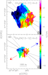 |
Fig. 5 Moment-9 maps of the CH3CN(12–11) K=3 (panel a) and 13CH3CN(13–12) K=3 (panel b) lines. The systemic velocity is ~−3.9 km s−1. The solid line shows the deconvolved direction of the major axis of the continuum emission, while the dashed lines give the errors on this direction. The blue and red arrows indicate the directions of the blue- and redshifted lobes of the jet shown in Fig. 1. The ellipses in the bottom right corners denote the synthesized beams. |
4 Data analysis
Although the disk and the associated jet (or outflow) in a YSO are tightly connected entities, for the sake of clarity, we analyze them separately, with our main aim being to shed light on their physical parameters and kinematical structure.
4.1 The jet
The higher sensitivity and angular resolution with respect to previous SiO observations of the jet (Su et al. 2011) allow us to improve our knowledge of its structure and velocity field. For this purpose, we adopt the model by Cesaroni et al. (1999), where the bipolar jet is described as a cone where the material is expanding radially with velocity proportional to the distance from the star. After fixing the PA of the jet axis to PAja=−60°, the free parameters of the model are the opening angle of the cone, θ, the angle between the axis of the cone and the plane of the sky, ϕ, and the velocity gradient V0/R0. A more detailed description is given in Appendix A. As done by Cesaroni et al. (1999), we only use the model to derive the borders of the region in space and velocity where SiO emission is present. We change the three input parameters of the model until these borders encompass the observed emission, thus deriving the main parameters of the flow.
While Cesaroni et al. (1999) constrained the model parameters using only the map of the jet and the PV diagram along the jet axis, we also use the PV diagrams perpendicular to the jet axis across the two bow shocks to the SE and NW. The result is shown in Fig. 6, where the map and PV plots of the SiO(5–4) line are compared to the borders obtained from the best-fit model. In practice, the best fit was obtained using the values derived by Cesaroni et al. (1999) as initial guesses and then varying these until a good match with the map and PV diagrams was found by eye. The resulting values are ϕ=3°, θ=10°, and V0/R0=10 km s−1 arcsec−1=1.3 km s−1 pc−1. The only significant difference with respect to the values obtained by Cesaroni et al. (1999) from lower resolution observations of the SiO(2–1) line (ϕ=9°, θ=21°, and V0/R0=8.3 km s−1 arcsec−1=1.3 km s−1 pc−1) is that the jet appears to be more collimated by a factor of ~2.
The PV plots across the bow shocks at the two ends of the jet (see bottom panels of Fig. 6) reveal that the SiO emission is indeed confined to the outer layer, and thus seems to be tracing the part of the cavity walls opened by the jet that corresponds to the post-shock region.
Further analysis of the jet can be performed by means of the H2CO lines. Given the different energies of the three lines (see Sect. 3.1), we could obtain maps of the rotational temperature, Trot, and column density, Ncol, of the H2CO molecule, assuming optically thin emission and local thermodynamic equilibrium (LTE). For this purpose, we used the maps of the integrated emission over the lines. In particular, we computed the ratio between the map of the (30,3–20,2) line and that obtained by averaging the maps of the (32,2–22,1) and (32,1–22,0) lines. The results are shown in Fig. 7, where only values with relative errors of <60% are displayed. We note that the method does not provide us with reliable values close to the (proto)star, where the emission is likely optically thick, and in part of the bow shocks, where the emission is too faint or the temperature is too high to be measured with transitions whose energies lie below 68 K. Despite these limitations, one sees that the bow shock to the NW presents a clear structure, where the maximum temperature and column density are attained along the leading edge, while the colder gas lies in the tail. As for the bow shock to the SE, H2CO emission is detected only in the trailing wake, which appears cooler and less dense. As a whole, this picture reveals differences in the evolution of the two lobes of the jet, where the NW lobe is still impinging on dense material, while the SE lobe has already pierced its way through a lower density medium.
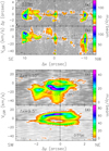 |
Fig. 6 SiO(5–4) line emission in IRAS 20126+4104. The offsets are relative to the phase center of the observations. (a) Moment-8 map of the emission rotated by 30° clockwise, so that the jet axis lies parallel to the X-axis of the plot. The dotted lines indicate the cuts used to make the PV diagrams in panels c and d. According to our conical jet model, emission can be seen only in the region comprised between the two dashed lines. The horizontal and vertical lines mark the position of the 1.4 mm continuum peak. (b) Moment-8 PV diagram along the jet axis. The dotted lines have the same meaning as in panel a. The cross in the bottom left corner indicates the angular and spectral resolutions. The vertical line marks the position of the continuum peak and the horizontal line the systemic velocity of −3.9 km s−1. (c) PV diagram along the dotted line at offset |
![Mathematical equation: $\[+9^{\prime\prime}_\cdot5\]$](/articles/aa/full_html/2025/01/aa52686-24/aa52686-24-eq9.png)
4.2 The disk
Previous studies of IRAS 20126+4104 (e.g., Palau et al. 2017) have shown that the disk is detected in COMs, the typical tracers of hot molecular cores (HMCs); although some emission in the same molecules is also detected from shocks at the base of the outflow. Our frequency setup covers many lines of COMs, but in the present article we focus only on methyl cyanide and its isotopologs ![Mathematical equation: $\[\mathrm{CH}_{3}^{13}\mathrm{CN}\]$](/articles/aa/full_html/2025/01/aa52686-24/aa52686-24-eq10.png) and 13CH3CN) and on the DCN(3–2) line, which appears to trace the disk over larger radii than CH3CN.
and 13CH3CN) and on the DCN(3–2) line, which appears to trace the disk over larger radii than CH3CN.
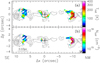 |
Fig. 7 Contour map of the SiO emission (same as in Fig. 1a) overlaid on maps of the H2CO rotational temperature (panel a) and column density (panel b). The maps have been rotated by 30° clockwise. The ellipse in the bottom right corner denotes the synthesized beam. The cross marks the position of the 1.4 mm continuum peak. |
4.2.1 Evidence for Keplerian rotation
In Fig. 8, we compare the PV diagrams along the disk plane in different lines. The PA of the plane of the disk was estimated to be PAd≃53° (Cesaroni et al. 2005) and we assume this value for our analysis. As noted by Cesaroni et al. (2005, 2014), the pattern of the PV plots has a “butterfly” shape, strongly suggestive of Keplerian rotation. To further support this interpretation, we fitted the emission in each channel of the CH3CN(12–11) K=3 component with a 2D Gaussian and in Fig. 9 we plot the peak positions thus obtained. We also draw ellipses corresponding to the deconvolved FWHM of the Gaussian fit. It is interesting to note that the orientation of the ellipses changes systematically going from the high velocities to the low velocities, with the latter ellipses oriented SE–NW and the former NE–SW.
This effect is better visualized in Fig. 10, where we plot the absolute value of the angle Θ between the major axis of the ellipses and the disk rotation axis, which is assumed to be perpendicular to the major axis of the continuum emission. This is done for the strongest and least blended lines indicated in the figure. By definition, Θ=90° for the continuum emission. The plot shows that, at high velocities, |Θ| is close to 90°, whereas close to the systemic velocity, |Θ| tends to 0°. Such behavior is expected in a Keplerian disk, as one can see from the template velocity pattern in Fig. 11, where the high-velocity red- and blueshifted emission arises from elongated regions perpendicular to the disk rotation axis, whereas the systemic velocity traces regions parallel to it.
4.2.2 Derivation of Trot and Ncol
To estimate some physical parameters of the disk, we rely on a large number of methyl cyanide lines with different excitation energies, which can be analyzed under the LTE approximation given the large densities (>107 cm−3; see e.g., Kurtz et al. 2000) typical of HMCs.
Thanks to the high resolution and sensitivity of our observations, we can improve on previous estimates of the temperature and column density (Cesaroni et al. 1997), which were only mean values over the whole disk. In particular, we wish to obtain the CH3CN rotational temperature, Trot, and column density, Ncol, as a function of radius in the disk. To this end, we use the PV diagrams of selected methyl cyanide lines with the approach described below.
Since the disk is undergoing Keplerian rotation, the emission in the PV plots is expected to have a “butterfly” shape, where the outer border of the pattern (i.e., the hyperbolic branches with the highest and lowest velocities) corresponds to the velocities at the intersection between the disk and the plane of the sky. Therefore, the emission along these two branches can be used to compute the physical parameters as a function of radius. The latter is simply the offset in the PV plot relative to the continuum position. However, the observed data result from the convolution of the butterfly-shaped pattern with the synthesized beam and the intrinsic line width, which makes it non-trivial to identify the above-mentioned hyperbolic branches. To overcome this problem, we decided to use an empirical method. We fitted the emission in the PV plot of the DCN line with a Gaussian, both for fixed velocity and for fixed offset, thus deriving, respectively, the offset and the velocity corresponding to the peak emission. We note that we chose the DCN line because this is detected at larger disk radii than the other transitions observed by us. The distribution of these peaks is shown in Fig. 12, where the white and black points indicate the peaks obtained with fixed velocity and fixed offset, respectively. With the exception of the central region of the plot (crosses), the other points (solid squares) describe two hyperbolic branches that we can use for our analysis.
For our calculation of Trot and Ncol, we selected only the lines of the main species that were least affected by blending with other transitions, namely the K = 2, 3, 4, 5, 7, 8 components and the v8=1 K, l = 2, 1 line. In cases where the line wings were overlapping with a nearby line, the channels affected by this blending were clipped. For each of these lines, a PV plot with the same grid of pixels was built and the line brightness temperature, TB, in each of the solid points in Fig. 12 was extracted. All these values of TB were fitted with the expression
![Mathematical equation: $\[T_{\mathrm{B}}^{\mathrm{mod}}=\eta ~T_{\text {rot }}\left(1-\mathrm{e}^{-\tau}\right),\]$](/articles/aa/full_html/2025/01/aa52686-24/aa52686-24-eq12.png) (1)
(1)
where η ≤ 1 is a filling factor and the line opacity is given by
![Mathematical equation: $\[\tau=\frac{1}{4 \pi \delta V} \sqrt{\frac{\ln 2}{\pi}} \frac{A_{u l} c^{3}}{\nu^{3}} g_{u} \frac{N_{\text {col }}}{Q(T_{\text {rot }})} \mathrm{e}^{-\frac{E_{u}}{k T_{\text {rot }}}}\left(\mathrm{e}^{\frac{h \nu}{k T_{\text {rot }}}}-1\right),\]$](/articles/aa/full_html/2025/01/aa52686-24/aa52686-24-eq13.png) (2)
(2)
where Aul is the Einstein coefficient, δV the channel width in velocity, c the speed of light, ν the line frequency, Q(Trot) the partition function, Eu the upper level energy, h the Planck constant, and k the Boltzmann constant. Here, we assume LTE and the best fit was obtained by minimizing the expression ![Mathematical equation: $\[{\sum}_{i}\left(T_{\mathrm{B} i}-T_{\mathrm{B} i}^{\mathrm{mod}}\right)^{2}\]$](/articles/aa/full_html/2025/01/aa52686-24/aa52686-24-eq14.png) , where the sum runs over the selected CH3CN lines (see above). For this purpose, the free variables η, Trot, and Ncol were varied over reasonable intervals. In this way, we obtained Trot and Ncol of CH3CN at each pixel of the PV plot, as shown in Figs. 13a and 13b. The calculation was done only for the pixels of the PV diagram where at least three lines were detected.
, where the sum runs over the selected CH3CN lines (see above). For this purpose, the free variables η, Trot, and Ncol were varied over reasonable intervals. In this way, we obtained Trot and Ncol of CH3CN at each pixel of the PV plot, as shown in Figs. 13a and 13b. The calculation was done only for the pixels of the PV diagram where at least three lines were detected.
Figures 13c and 13d show Trot and Ncol as functions of the angular radius θ obtained directly from the offset in Figs. 13a and 13b. Finally, from linear fits to the data, we derive the relations
![Mathematical equation: $\[T_{\mathrm{rot}}(\mathrm{~K}) =~107~[\theta(\operatorname{arcsec})]^{-0.32}=1140~~[R(\mathrm{au})]^{-0.32}\]$](/articles/aa/full_html/2025/01/aa52686-24/aa52686-24-eq15.png) (3)
(3)
![Mathematical equation: $\[N_{\mathrm{col}}(\mathrm{~cm}^{-2}) =1.1 \times 10^{15}~[\theta(\operatorname{arcsec})]^{-1.3}=1.7 \times 10^{19}~[R(\mathrm{au})]^{-1.3}.\]$](/articles/aa/full_html/2025/01/aa52686-24/aa52686-24-eq16.png) (4)
(4)
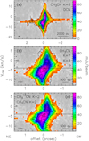 |
Fig. 8 Moment-8 PV diagrams of various molecular transitions along the disk plane (PA=53°). The offset is relative to the phase center of the observations. The horizontal and vertical lines mark the systemic velocity and the position of the 1.4 mm continuum peak, respectively. The crosses in the bottom left corners indicate the angular and spectral resolutions. (a) PV plot of the CH3CN(12–11) K=3 component (contours) overlaid on that of the DCN(3–2) line. Contour levels range from 7 to 91 in steps of 12 mJy/beam. (b) Same as panel a, with CH3CN(12–11) K=7 overlaid on K=3. Contour levels range from 5 to 53 in steps of 6 mJ /beam. (c) Same as panel a, but with |
![Mathematical equation: $\[\mathrm{CH}_{3}^{13}\mathrm{CN}\]$](/articles/aa/full_html/2025/01/aa52686-24/aa52686-24-eq11.png)
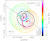 |
Fig. 9 Distribution of the peaks (colored points) obtained by fitting a 2D Guassian to the emission in each channel of the channel maps of the CH3CN(12–11) K=3 line. The colored ellipses are the deconvolved FWHM of the fitted Gaussians. The color corresponds to the LSR velocity as indicated by the scale to the right. The black cross and ellipse represent the peak position and deconvolved FWHM of the 1.4 mm continuum emission, respectively. The dashed line outlines the direction of the major axis of the black ellipse. The shaded ellipse in the bottom right corner represents the synthesized beam. |
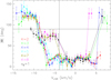 |
Fig. 10 Absolute value of the angle between the major axis of the deconvolved FWHM of the emission in the line channel, and the axis of the disk versus the LSR velocity of the channel. The colors correspond to the CH3CN(12–11) lines as indicated in the figure. The vertical line marks the systemic velocity. The horizontal line corresponds to |Θ| = 90°. |
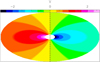 |
Fig. 11 Schematic plot of the velocity along the line of sight relative to the star velocity, in a template Keplerian disk inclined by 30°. The plane of the figure is the plane of the sky and the dashed line is the projection of the disk rotation axis. The color scale indicating the velocity is in arbitrary units. We note that the high-velocity magenta/red and blue patterns are elongated perpendicular to the yellow/green patterns, which correspond to velocities close to zero. |
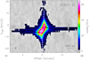 |
Fig. 12 Moment-8 PV diagram of the DCN(3–2) line emission along the plane of the disk (PA=53°). The offset is relative to the phase center of the observations. The black and white points mark the emission peaks obtained by fitting a Gaussian to the emission, respectively, for fixed offset and fixed velocity. The solid squares indicate the points selected by us to define the velocity–radius relation in the Keplerian disk. |
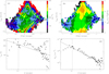 |
Fig. 13 Analysis of the temperature and column density distribution in the disk around IRAS 20126+4104. (a) PV diagram along the disk plane of the CH3CN rotation temperature obtained by fitting the brightness temperature of selected transitions. The black solid squares mark the points used to derive Trot as a function of radius (see text). (b) Same as panel a but for the CH3CN column density. (c) Rotation temperature versus angular radius obtained from the points of the PV diagram marked by the black solid squares. The solid line is a linear fit to the data corresponding to the relation Trot(K) = 107 [θ(arcsec)]−0.32. The dashed line corresponds to half the synthesized beam. (d) Same as panel c but for the CH3CN column density. The relationship obtained from the linear fit to the data is Ncol(cm−2) = 1.1 × 10¹⁵ [θ(arcsec)]−1.3. |
4.2.3 Evidence for infall
In addition to rotation, the presence of accretion in the disk is suggested by the shape of the PV plots, because for Keplerian rotation no emission should be seen either at redshifted velocities and positive offsets (with respect to the position of the star) or at blueshifted velocities and negative offsets. This is clearly not true for the PV diagrams in Fig. 8. It must be noted that the emission in these two quadrants of the PV plots cannot be explained with smearing due to the finite spectral and angular resolution. If this were the case, in Fig. 8c, the emission at offset ![Mathematical equation: $\[-0^{\prime\prime}_\cdot33\]$](/articles/aa/full_html/2025/01/aa52686-24/aa52686-24-eq17.png) and velocity −7 km s−1, for example, would be attenuated by 3 × 10⁻³ times in space (for HPBW≃
and velocity −7 km s−1, for example, would be attenuated by 3 × 10⁻³ times in space (for HPBW≃![Mathematical equation: $\[0^{\prime\prime}_\cdot16\]$](/articles/aa/full_html/2025/01/aa52686-24/aa52686-24-eq18.png) ) and 5 × 10⁻² times in velocity (assuming an intrinsic line FWHM=3 km s−1). These factors are too small to allow for the intensity of 22 mJy/beam measured at that point, taking into account the fact that the maximum intensity in the PV plot is 97 mJ/beam. The effect of adding a radial velocity component to Keplerian rotation is described by Eq. (1) of Cesaroni et al. (2011); in particular, their Fig. 13 illustrates the pattern expected in the PV diagram.
) and 5 × 10⁻² times in velocity (assuming an intrinsic line FWHM=3 km s−1). These factors are too small to allow for the intensity of 22 mJy/beam measured at that point, taking into account the fact that the maximum intensity in the PV plot is 97 mJ/beam. The effect of adding a radial velocity component to Keplerian rotation is described by Eq. (1) of Cesaroni et al. (2011); in particular, their Fig. 13 illustrates the pattern expected in the PV diagram.
Further possible evidence of infall comes from a noticeable feature of the PV plots in Figs. 8b and 8c, where we note a striking difference between the peak of the emission in lines with different opacities and excitation energies. For instance, the CH3CN K=2 component peak is blueshifted, whereas the K=2 line of the ![Mathematical equation: $\[\mathrm{CH}_{3}^{13} \mathrm{CN}\]$](/articles/aa/full_html/2025/01/aa52686-24/aa52686-24-eq19.png) isotopolog and the CH3CN K=8 line peak at redshifted velocities. This behavior is evident in Fig. 14, where we plot the velocity of the peak in the PV diagram as a function of the excitation energy of the transition for the least blended CH3CN lines with the best S/N. Clearly, the higher the excitation energy, the more redshifted the emission. While several explanations are possible, at the end of Sect. 4.2.4 we propose that this trend is due to the presence of accretion.
isotopolog and the CH3CN K=8 line peak at redshifted velocities. This behavior is evident in Fig. 14, where we plot the velocity of the peak in the PV diagram as a function of the excitation energy of the transition for the least blended CH3CN lines with the best S/N. Clearly, the higher the excitation energy, the more redshifted the emission. While several explanations are possible, at the end of Sect. 4.2.4 we propose that this trend is due to the presence of accretion.
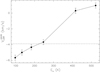 |
Fig. 14 LSR velocity corresponding to the peak emission in the PV diagrams of the CH3CN(12–11) K = 2, 3, 4, 5, 7, 8 lines as a function of the upper energy of the transition. The dashed line marks the systemic LSR velocity of −3.9 km s−1. |
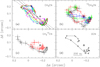 |
Fig. 15 Distributions of the peaks of the emission in the velocity channels of various lines observed in IRAS 20126+4104. The error bars are the formal errors on the Gaussian fits. The offsets are relative to the phase center of the observations. The black cross marks the position of the 1.4 mm continuum peak. (a) Plot obtained from the CH3CN(12–11) lines. The color coding is as follows: K=2 black, 3 red, 4 green, 5 blue, 7 cyan, 8 yellow, and v8=1 magenta. The dashed lines are linear fits to the points obtained by fitting Y vs X and X vs Y; the solid line is the mean of the two. (b) Same as panel a but for the 13CH3CN(13–12) components: K=2 black, 3 red, 4 green, and 5 blue. (c) Same as panel a but for the |
![Mathematical equation: $\[\mathrm{CH}_{3}^{13} \mathrm{CN}\]$](/articles/aa/full_html/2025/01/aa52686-24/aa52686-24-eq20.png)
4.2.4 A model for the disk
An intriguing feature of the disk in IRAS 20126+4104 is the distribution of the emission peaks in Fig. 15. As already noted by Cesaroni et al. (2014), the positions of the peaks of the methyl cyanide lines at different velocities are not aligned along a straight line passing through the disk center, but describe a C-shaped structure. The case of IRAS 20126+4104 is not unique because the same C-shaped pattern has also been found by Sánchez-Monge et al. (2013) and Bayandina et al. (2024) in two similar objects. Here, we propose a toy model that can qualitatively explain the shape of these plots as well as the trend of the peak velocity with energy of the line.
The model is intended to be a proof of concept to explain the results illustrated in Figs. 9, 14, and 15. Briefly, we propose that such results are due to the presence of a dusty envelope enshrouding the disk itself. We assume a simple scenario with a geometrically thin disk and a spherical halo extending from the center up to the outer radius of the disk. The density of the halo is ∝ r−1, where r is the distance from the disk center. The disk is dust-free and optically thick in the line emission, whereas the line emission and absorption in the dusty halo are negligible. Incidentally, we note that, while the outflow carves a cavity in the spherical halo, it is likely to be collimated enough not to affect the spherical assumption for the radiative transfer modeling we perform. We also assume that the disk is undergoing Keplerian rotation and radial infall with velocity ∝ r−1/2. The model is described in Appendix B.
The best fit to the data is obtained in two steps: first, we fit the observed LSR velocity of the disk as in Sánchez-Monge et al. (2013), thus determining all parameters except the envelope opacity; then we vary this opacity until we reproduce the C-shaped distribution of the peaks. Below, we describe these two steps one by one.
Fit of the LSR velocity
To fit the disk velocity field, we minimize the expression ![Mathematical equation: $\[{\sum}_{i}\left(V_{i}^{\mathrm{obs}}-V_{i}^{\mathrm{mod}}\right)^{2}\]$](/articles/aa/full_html/2025/01/aa52686-24/aa52686-24-eq21.png) , where
, where ![Mathematical equation: $\[V_{i}^{\mathrm{obs}}\]$](/articles/aa/full_html/2025/01/aa52686-24/aa52686-24-eq22.png) is the LSR velocity of a peak in Fig. 15 and
is the LSR velocity of a peak in Fig. 15 and ![Mathematical equation: $\[V_{i}^{\text {mod }}\]$](/articles/aa/full_html/2025/01/aa52686-24/aa52686-24-eq23.png) is the LSR velocity computed from Eq. (B.1) at the position of that peak. We decided to use only the peaks of the CH3CN ground-state K components in Fig. 15a, because these have the best S/N and consequently the smallest positional errors. As explained in Appendix B.1, the input variables of the disk model are the coordinates of the star (Xs, Ys), the systemic velocity (Vsys), the PA of the projected major axis of the disk (PAd), the angle between the disk plane and the plane of the sky (ψ), the mass of the star (Ms), and the ratio (A) between the radial (i.e., infall) velocity and the rotation velocity. We fixed PAd to the value obtained from a least-square fit to the peaks of all ground-state K lines in Fig. 15 a (48°±6°). The other parameters were varied over suitable ranges. The best fit was obtained for
is the LSR velocity computed from Eq. (B.1) at the position of that peak. We decided to use only the peaks of the CH3CN ground-state K components in Fig. 15a, because these have the best S/N and consequently the smallest positional errors. As explained in Appendix B.1, the input variables of the disk model are the coordinates of the star (Xs, Ys), the systemic velocity (Vsys), the PA of the projected major axis of the disk (PAd), the angle between the disk plane and the plane of the sky (ψ), the mass of the star (Ms), and the ratio (A) between the radial (i.e., infall) velocity and the rotation velocity. We fixed PAd to the value obtained from a least-square fit to the peaks of all ground-state K lines in Fig. 15 a (48°±6°). The other parameters were varied over suitable ranges. The best fit was obtained for ![Mathematical equation: $\[X_{\mathrm{s}}=20^{\mathrm{h}} 14^{\mathrm{m}} 26^\text{s}_\cdot025, Y_{\mathrm{s}}{=}41^{\circ} 13^{\prime} 32^{\prime \prime}_\cdot60\]$](/articles/aa/full_html/2025/01/aa52686-24/aa52686-24-eq24.png) , Vsys=−4.3 km s−1, ψ=59°, Ms=12 M⊙, and A=0.42.
, Vsys=−4.3 km s−1, ψ=59°, Ms=12 M⊙, and A=0.42.
A comparison between the data and the model is shown in Fig. 16, where the ellipse is the projection of the disk on the plane of the sky and the circles are the observed CH3CN peaks. The color indicates the component of the velocity along the line of sight (LOS) and the agreement between model and data is good where the color of the point matches that of the disk model at the same position. Overall, the fit is satisfactory and proves that a non-negligible radial velocity component (i.e., A > 0) is needed to reproduce the observed velocities. However, a significant discrepancy between model and data is visible at the most red-shifted velocities, suggesting that the SW part of the disk must be perturbed. We discuss this issue in Sect. 5.
Fit of the C-shaped pattern
Now that we have a reasonable disk model, we can propose an explanation of the C-shaped structures shown in Figs. 9 and 15. The underlying hypothesis is that the emission from the part of the disk lying beyond the plane of the sky passing through the disk center is more absorbed than that lying closer to the observer. This hypothesis is supported by Fig. 17, where we show the velocity patterns of the disk overlaid on the map of the dust optical depth of the envelope between the disk and the observer – computed from Eq. (B.9). We note that the largest opacities are found for positive values of Δy, which favors the emission for Δy < 0. Therefore, when we fit the line emission in each velocity channel with a 2D Gaussian, the peak position tends to be skewed towards negative Δy. This effect is important for the low-velocity emission (green and yellow patterns in the figure) which is extended but becomes progressively negligible at high velocities (red and blue patterns) because the emission is more and more compact. This can explain why the blue- and redshifted peaks in Fig. 9 lie close to the major axis of the projected disk plane, whereas the lower-velocity peaks are shifted to the SE.
To prove that our explanation is viable, we used our model with the best-fit parameters obtained above to generate a disk with surface temperature computed from Eq. (3). We also fix the disk radius to half the maximum size of the peak distribution in Fig. 15, namely ![Mathematical equation: $\[R_{\mathrm{d}}{=}0^{\prime\prime}_\cdot3{=}490\]$](/articles/aa/full_html/2025/01/aa52686-24/aa52686-24-eq25.png) au. As we assume the line emission to be optically thick all over the disk, the observed peak line brightness temperature at a given radius is equal to the kinetic temperature at this radius attenuated by the absorption through the dusty envelope according to Eq. (B.5). For our calculations, we assumed a Gaussian line profile with FWHM of 4 km s−1. To make the comparison with the observations more realistic, we also convolved the disk+envelope model with the beam of our observations and fitted the resulting cube channel by channel with a 2D Gaussian, as done for the data. In this process, the only free parameter is the opacity of the envelope, that is, the value of τ0 (see Appendix B.2), which was varied until a reasonable match between the observed peak TB and that obtained from the model was achieved for τ0 = 0.4. We note that the result holds for any line because we assume the line emission from the disk to be optically thick.
au. As we assume the line emission to be optically thick all over the disk, the observed peak line brightness temperature at a given radius is equal to the kinetic temperature at this radius attenuated by the absorption through the dusty envelope according to Eq. (B.5). For our calculations, we assumed a Gaussian line profile with FWHM of 4 km s−1. To make the comparison with the observations more realistic, we also convolved the disk+envelope model with the beam of our observations and fitted the resulting cube channel by channel with a 2D Gaussian, as done for the data. In this process, the only free parameter is the opacity of the envelope, that is, the value of τ0 (see Appendix B.2), which was varied until a reasonable match between the observed peak TB and that obtained from the model was achieved for τ0 = 0.4. We note that the result holds for any line because we assume the line emission from the disk to be optically thick.
The distribution of the peaks obtained with our procedure is compared in Fig. 18 to the peaks of the CH3CN ground-state lines of Fig. 15a. We conclude that the model qualitatively mimics the C-shaped distribution of the data peaks, lending support to our interpretation.
We believe that the proposed scenario could also explain the velocity drift in Fig. 14. As the part of the disk where the envelope opacity is maximum is also the part of the disk where the infalling velocity is blueshifted (see Fig. 17), this causes the line profile to become skewed, whose blueshifted part is attenuated with respect to the redshifted part. This effect must be more pronounced for the higher-energy transitions, because they trace more internal regions, which are denser and as such more affected by dust absorption. The result is that these lines appear more redshifted than the lower-energy transitions.
Finally, it is worth computing the envelope mass. This is related to τ0 through the expression
![Mathematical equation: $\[M_{\text {env }}=2 \pi \frac{\tau_{0}}{K_{\mathrm{d}}} R_{\mathrm{d}}^{2} \simeq 6.7 ~M_{\odot},\]$](/articles/aa/full_html/2025/01/aa52686-24/aa52686-24-eq26.png) (5)
(5)
where κd is the dust absorption coefficient that we assume to be equal to 0.01 cm2 g−1. A comparison between this value and the mass estimate obtained from the continuum flux density measured by us (~280 mJy) is unreliable for two reasons. First, the calculation requires knowledge of the halo dust temperature. Second, a substantial fraction of the continuum emission is resolved out by the interferometer, meaning that the mass estimated from the continuum flux density is a lower limit. Vice versa, the mass computed from Eq. (5) is not affected by this problem because τ0 takes into account the dust absorption due to the whole envelope being crossed by the LOS.
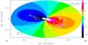 |
Fig. 16 Peaks of the CH3CN(12–11) K = 2, 3, 4, 5, 7, 8 components in the different velocity channels overlaid on the best-fit model of a disk undergoing Keplerian rotation and radial infall (see text). The data have been rotated counterclockwise by 42° to align the disk with the X-axis. The offsets are relative to the disk center. The color indicates the velocity along the line of sight relative to the star. The black cross marks the position of the 1.4 mm continuum peak. |
 |
Fig. 17 Maps of the velocity and dust opacity over the disk according to our model. The black ellipse outlines the border of the disk and the color-coded patterns are the loci of points of the disk with the same velocity along the line of sight, ranging from −10 to +10 in steps of 1 km s−1. The gray scale with dotted contours is a map of the envelope dust opacity. |
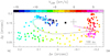 |
Fig. 18 Comparison between the peaks of the CH3CN(12–11) K = 2, 3, 4, 5, 7, 8 components in the different velocity channels (solid circles) and those obtained from the model for a template line (empty circles connected by the solid line). We note that the model peak distribution qualitatively reproduces the C-shaped pattern described by the data. The system is rotated clockwise by 42° and the offsets are relative to the phase center of the observations. The color indicates the LSR velocity. The black square marks the center of the disk according to the model. The black cross indicates the position of the 1.4 mm continuum peak with error bars. |
5 Discussion
The analysis performed in the previous sections provides us with some hints as to the nature and evolutionary phase of IRAS 20126+4104. First of all, we note that the proposed model to explain the C-shaped structure of the peak distribution only holds if the disk is inclined in such a way that the NW part of it lies beyond the star with respect to the observer. It is only in this case that the opacity plotted in Fig. 17 is maximum to the NW and the arc of the C-shaped structure points to the SE, as observed. The orientation of the jet suggests that this is indeed the disk inclination, because the blueshifted lobe is pointing to the NW. Interestingly, the other two sources for which a similar C-shaped distribution has been found – G35.20–0.74 N (Sánchez-Monge et al. 2013) and G11.92–0.61 MM1 (Bayandina et al. 2024) – do not satisfy the same requirement, because the arc points towards the blue lobe of the associated jet. We speculate that this difference is due to the lack of a thick envelope around these two sources, and that the C-shape might be caused by self-absorption due to a large line opacity in a geometrically thick disk. In this scenario, IRAS 20126+4104 should be more embedded and thus presumably less evolved than G35.20–0.74 N and G11.92–0.61 MM1.
If the source is indeed young and massive, the accretion rate should also be high. This can be estimated from Eq. (4) of Cesaroni et al. (1999), which in our case takes the form
![Mathematical equation: $\[\dot{M}_{\mathrm{acc}}=2 \pi R_{\mathrm{d}} ~\mu \mathrm{m}_{\mathrm{H}} \frac{N_{\mathrm{col}}(R_{\mathrm{d}})}{X_{\mathrm{CH}_{3} \mathrm{CN}}} \cos ~\psi ~A \sqrt{\frac{G M_{\mathrm{s}}}{R_{\mathrm{d}}}},\]$](/articles/aa/full_html/2025/01/aa52686-24/aa52686-24-eq27.png) (6)
(6)
where μ=2.8 is the mean molecular weight, mH the mass of the hydrogen atom, G the gravitational constant, XCH3CN the CH3CN abundance relative to H2, cos ψ a correction factor due to the inclination of the disk, and Ncol is given by Eq. (4). For Ms=12 M⊙, ![Mathematical equation: $\[R_{\mathrm{d}}{=}0^{\prime\prime}_\cdot3{=}490\]$](/articles/aa/full_html/2025/01/aa52686-24/aa52686-24-eq28.png) au, A=0.42 (see Sect. 4.2.4), and XCH3CN=10−9, we obtain
au, A=0.42 (see Sect. 4.2.4), and XCH3CN=10−9, we obtain ![Mathematical equation: $\[\dot{M}_{\text {acc }} \simeq 1.7 \times 10^{-3} ~M_{\odot} ~\mathrm{yr}^{-1}\]$](/articles/aa/full_html/2025/01/aa52686-24/aa52686-24-eq29.png) , a value in reasonable agreement with that obtained by Cesaroni et al. (1999) from the millimeter continuum emission and the spread in peak velocity among different CH3CN lines (P~9.8 × 10⁻⁴ M⊙ yr−1).
, a value in reasonable agreement with that obtained by Cesaroni et al. (1999) from the millimeter continuum emission and the spread in peak velocity among different CH3CN lines (P~9.8 × 10⁻⁴ M⊙ yr−1).
The expressions of Trot and Ncol in Eqs. (3) and (4) can also be used to estimate the Toomre Q parameter (Toomre 1964) and hence investigate the disk stability. In our case, we have
![Mathematical equation: $\[Q=\sqrt{\frac{M_{\mathrm{s}}}{G R^{3}}} \frac{\sigma_{\mathrm{v}} ~X_{\mathrm{CH}_{3} \mathrm{CN}}}{\pi ~\mu \mathrm{m}_{\mathrm{H}} N_{\mathrm{col}}},\]$](/articles/aa/full_html/2025/01/aa52686-24/aa52686-24-eq30.png) (7)
(7)
where σv is the velocity dispersion. A lower limit on Q can be obtained assuming that σv contains only a thermal contribution, hence ![Mathematical equation: $\[\sigma_{\mathrm{v}}=\sqrt{3 k T_{\mathrm{K}} /(\mu \mathrm{m}_{\mathrm{H}})}\]$](/articles/aa/full_html/2025/01/aa52686-24/aa52686-24-eq31.png) , where TK is kinetic temperature. Since the CH3CN molecule is likely thermalized at the disk densities, we further assume TK=Trot and can thus calculate the lower limit on Q as a function of the radius R in the disk:
, where TK is kinetic temperature. Since the CH3CN molecule is likely thermalized at the disk densities, we further assume TK=Trot and can thus calculate the lower limit on Q as a function of the radius R in the disk:
![Mathematical equation: $\[Q>1.5\left(\frac{R}{R_{\mathrm{d}}}\right)^{-0.36}.\]$](/articles/aa/full_html/2025/01/aa52686-24/aa52686-24-eq32.png) (8)
(8)
Since by definition R < Rd, one has Q > 1 at all radii, which implies that the disk is stable.
It is also interesting to compute the angle between the axis of the disk and that of the jet. Using the same notation as in the Appendices, we can express the directions of the two axes by means of the unit vectors ![Mathematical equation: $\[\hat{e}_\text{j}\]$](/articles/aa/full_html/2025/01/aa52686-24/aa52686-24-eq33.png) = (sin PAja cos ϕ, cos PAja cos ϕ, − sin ϕ) for the jet and
= (sin PAja cos ϕ, cos PAja cos ϕ, − sin ϕ) for the jet and ![Mathematical equation: $\[\hat{e}_\text{d}\]$](/articles/aa/full_html/2025/01/aa52686-24/aa52686-24-eq34.png) = (sin PAda sin ψ, cos PAda sin ψ, − cos ψ) for the disk, where PAja=−60°, ϕ=3°, PAda=−42°, and ψ=59°. The angle between the two axes is thus equal to arccos(
= (sin PAda sin ψ, cos PAda sin ψ, − cos ψ) for the disk, where PAja=−60°, ϕ=3°, PAda=−42°, and ψ=59°. The angle between the two axes is thus equal to arccos(![Mathematical equation: $\[\hat{e}_\text{j}\]$](/articles/aa/full_html/2025/01/aa52686-24/aa52686-24-eq35.png) ·
· ![Mathematical equation: $\[\hat{e}_\text{d}\]$](/articles/aa/full_html/2025/01/aa52686-24/aa52686-24-eq36.png) ) ≃ 33°. Interestingly, this value is very similar to the opening angle of the precession cone (37°) estimated by Cesaroni et al. (2005). This result lends further support to the scenario proposed by Shepherd et al. (2000), Cesaroni et al. (2005), and Caratti o Garatti et al. (2008), which invokes the existence of precession to explain the S-shaped morphology of the jet from IRAS 20126+4104.
) ≃ 33°. Interestingly, this value is very similar to the opening angle of the precession cone (37°) estimated by Cesaroni et al. (2005). This result lends further support to the scenario proposed by Shepherd et al. (2000), Cesaroni et al. (2005), and Caratti o Garatti et al. (2008), which invokes the existence of precession to explain the S-shaped morphology of the jet from IRAS 20126+4104.
As proposed by Shepherd et al. (2000), the precession could be caused by tidal interactions with a lower-mass nearby (proto)star. This hypothesis is consistent with the observed structure of the disk as revealed by the peak distributions in Fig. 15. Independently of the tracer, in this figure the distribution of the peaks is clearly asymmetric with respect to the continuum peak and the points appear to thicken on the SW side of it, whereas on the NE side they describe a more extended pattern. This effect is even more clear in Fig. 18, where the largest discrepancy between the model and the observed peaks is seen to the SW. A possible explanation for this asymmetry could be related to the perturbing action of a nearby star lying to the SW of IRAS 20126+4104. The existence of such a star is indeed suggested by the thermal jet detected at centimeter wavelengths to the south of IRAS 20126+4104 (Hofner et al. 1999, 2007) and is supported by the detection of a cluster of embedded YSOs in the area surrounding IRAS 20126+4104 (Montes et al. 2015).
An alternative explanation for the perturbed structure of the redshifted CH3CN emission to the SW is that in this region the dense gas traced by methyl cyanide is lifted from the disk plane by the jet. This possibility is suggested by the comparison between the CH3CN peaks and the SiO emission (see Fig. 19). The latter appears to peak precisely in the gap of the C-shaped CH3CN pattern, where the continuum peak is located, and the redshifted peaks are distributed along the SW side of the SiO jet. Indeed, a tight interaction between the material rotating in the disk and that expanding in the jet was also suggested by the LSR velocity and proper motions of the H2O masers (see Fig. 10 of Cesaroni et al. 2014). Therefore, we cannot exclude that a mechanism similar to that operating in disk winds is affecting the structure of the circumstellar disk in IRAS 20126+4104.
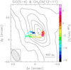 |
Fig. 19 Overlay of the CH3CN peaks (circles) on the moment-8 map (contours) of the SiO(5–4) line emission. The colored points and black cross are the same as in Fig. 18. The maps have been rotated by 42° counterclockwise for consistency with Fig. 18 and the offsets are relative to the phase center of the observations. The contour levels range from 6 to 36 in steps of 5 mJy/beam. The ellipse in the bottom left corner denotes the synthesized beam of the SiO map. |
6 Summary and conclusions
We report ALMA observations of the disk+jet system in the massive (proto)star IRAS 20126+4104, with a substantial improvement on previous observations at the same wavelengths with other instruments. The new data allow us to better define the geometrical and kinematical parameters of the jet and to obtain maps of the temperature and column density in the bow-shock regions at the tips of the jet lobes. As expected, both quantities decrease moving away from the shocks in the trailing wake of the flow. Our high-resolution images of the disk make it possible to derive the rotation temperature and column density of the CH3CN molecule as a function of radius. We also show that the disk is not only undergoing Keplerian rotation, but also has an inward velocity component implying an accretion rate of ~10−3 M⊙ yr−1, which is consistent with previous estimates obtained by other means. With this knowledge of the physical structure and velocity field of the disk, we were able to evaluate the Toomre Q parameter, which indicates that stability is attained at all radii. Finally, we propose that the disk morphology observed in high-density tracers might be caused by a dusty envelope enshrouding the disk itself. Our analysis also reveals the existence of a significant deviation from axial symmetry in the SW part of the disk, which might be caused by a nearby, lower-mass companion or could be the result of disk material being dragged into expansion along the jet.
Acknowledgements
V.M.R. acknowledges support from the grant PID2022-136814NB-I00 by the Spanish Ministry of Science, Innovation and Universities/State Agency of Research MICIU/AEI/10.13039/501100011033 and by ERDF, UE; the grant RYC2020-029387-I funded by MICIU/AEI/10.13039/501100011033 and by “ESF, Investing in your future”, and from the Consejo Superior de Investigaciones Científicas (CSIC) and the Centro de Astrobiología (CAB) through the project 20225AT015 (Proyectos intramurales especiales del CSIC); and from the grant CNS2023-144464 funded by MICIU/AEI/10.13039/501100011033 and by “European Union NextGenerationEU/PRTR”. A.S.-M. acknowledges support from the RyC2021-032892-I grant funded by MCIN/AEI/10.13039/501100011033 and by the European Union ‘Next GenerationEU’/PRTR, as well as the program Unidad de Excelencia María de Maeztu CEX2020-001058-M, and support from the PID2020-117710GB-I00 (MCI-AEI-FEDER, UE). This paper makes use of the following ALMA data: ADS/JAO.ALMA#2016.1.00595.S and ADS/JAO.ALMA#2019.1.00199.S. ALMA is a partnership of ESO (representing its member states), NSF (USA) and NINS (Japan), together with NRC (Canada), NSC and ASIAA (Taiwan), and KASI (Republic of Korea), in cooperation with the Republic of Chile. The Joint ALMA Observatory is operated by ESO, AUI/NRAO and NAOJ.
Appendix A Jet model
The jet model adopted by us is the same as the one presented by Cesaroni et al. (1999). It consists of a cone with opening angle θ and axis inclined by ϕ on the plane of the sky. Figure A.1 shows a sketch, where we have chosen a coordinate system (x, y, z) with z parallel to the LOS and x coincident with the projection of the cone axis on the plane of the sky. The gas inside the cone is expanding with radial velocity V proportional to the distance R from the vertex (i.e., from the position of the star), according to the expression
![Mathematical equation: $\[\boldsymbol{V}=V_{0} \frac{\boldsymbol{R}}{R_{0}}\]$](/articles/aa/full_html/2025/01/aa52686-24/aa52686-24-eq37.png) (A.1)
(A.1)
where V0 is the expansion speed at an arbitrary radius R0. We stress that our model is only sensitive to the ratio V0/R0.
We want to use the jet model to estimate the borders of the region inside which emission is expected and compare it to the data, both in space and velocity, to obtain the values of θ, ϕ, and V0/R0. On the plane of the sky, such a region is represented by the gray area in Fig. A.1a. Comparison with the PV diagrams requires calculating the maximum/minimum observed velocities attainable at a given position x, y. The projection of the velocity along the LOS depends only on the projection of vector R, hence the observed LSR velocity is
![Mathematical equation: $\[V_{\text {LSR }}=V_{\mathrm{sys}}+V_{\mathrm{z}}=V_{\mathrm{sys}}+\frac{V_{0}}{R_{0}} z\]$](/articles/aa/full_html/2025/01/aa52686-24/aa52686-24-eq38.png) (A.2)
(A.2)
with Vsys = −3.9 km s−1 systemic LSR velocity. Consequently, at a given position x, y the maximum/minimum values of the observed velocity are attained for the maximum/minimum values of z across the cone, i.e., on the surface of the cone. To calculate these values we consider the expression of the cone in the coordinate system (x′, y′, z′) where z′ is the axis of the cone (see Fig. A.1b):
![Mathematical equation: $\[z^{\prime 2} \tan ^{2} \theta=x^{\prime 2}+y^{\prime 2}.\]$](/articles/aa/full_html/2025/01/aa52686-24/aa52686-24-eq39.png) (A.3)
(A.3)
By applying the transformation of coordinates
![Mathematical equation: $\[\begin{aligned}x^{\prime} & =x ~\sin~ \phi-z ~\cos~ \phi \\y^{\prime} & =y \\z^{\prime} & =z ~\cos~ \phi+z ~\sin~ \phi\end{aligned}\]$](/articles/aa/full_html/2025/01/aa52686-24/aa52686-24-eq40.png) (A.4)
(A.4)
after some algebra one obtains the equation of the cone in the (x, y, z) coordinate system
![Mathematical equation: $\[z_{ \pm}=\frac{x ~\sin~ \phi ~\cos~ \phi \pm ~\cos~ \theta \sqrt{F(x, y; \theta, \phi)}}{\cos ^{2} \theta-\sin ^{2} \phi}\]$](/articles/aa/full_html/2025/01/aa52686-24/aa52686-24-eq41.png) (A.5)
(A.5)
where we have defined
![Mathematical equation: $\[F \equiv x^{2} \sin ^{2} \theta+y^{2}\left(\sin ^{2} \phi-\cos ^{2} \theta\right).\]$](/articles/aa/full_html/2025/01/aa52686-24/aa52686-24-eq42.png) (A.6)
(A.6)
The maximum/minimum velocities can be calculated by substituting Eq. (A.5) into Eq. (A.2).
The projection θ′ of angle θ on the plane of the sky (Fig. A.1a) is obtained for F = 0 because in this case there must be only one intersection between the LOS and the cone. This gives
![Mathematical equation: $\[\theta^{\prime}=\arctan \left(\frac{\sin \theta}{\sqrt{\cos ^{2} \theta-\sin ^{2} \phi}}\right).\]$](/articles/aa/full_html/2025/01/aa52686-24/aa52686-24-eq43.png) (A.7)
(A.7)
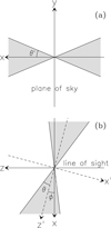 |
Fig. A.1 Sketch of the proposed conical model for the jet. a. View of the jet in projection onto the plane of the sky. We indicate the apparent opening angle with θ′. b. Projection of the jet onto the x, z plane. Here θ is the true opening angle and ϕ the inclination angle of the jet axis with respect to the plane of the sky. The observer lies at z = −∞. The z′ axis coincides with the axis of the cone, while we choose y′ = y. |
The previous equations allowed us to compute the border of the emitting region both in the x, y plane and in the x, VLSR (for y = 0) and y, VLSR (for fixed x) PV diagrams. This pattern was then compared to the data by eye and the input parameters θ, ϕ, and V0/R0 were varied until a reasonable match with the observed emission was obtained (see Fig. 6). As initial guesses for this procedure we used the values obtained by Cesaroni et al. (1999), namely ϕ=9°, θ=21°, and V0/R0=8.3 km s−1 arcsec−1. We also adopted a PA of the jet axis PAja=−60° and assumed that the position of the star was that of the 1.4 mm continuum peak, i.e., ![Mathematical equation: $\[\alpha(\mathrm{J} 2000){=}20^{\mathrm{h}} 14^{\mathrm{m}} 26^\text{s}_\cdot022\]$](/articles/aa/full_html/2025/01/aa52686-24/aa52686-24-eq44.png) and
and ![Mathematical equation: $\[\delta(\mathrm{J} 2000){=}41^{\circ} 13^{\prime} 32^{\prime \prime}_\cdot 58\]$](/articles/aa/full_html/2025/01/aa52686-24/aa52686-24-eq45.png) (see Sect. 3.2). The best fit was obtained for θ=10°, ϕ=3°, and V0/R0=10 km s−1 arcsec−1.
(see Sect. 3.2). The best fit was obtained for θ=10°, ϕ=3°, and V0/R0=10 km s−1 arcsec−1.
Appendix B Disk+halo model
To explain the C-shaped pattern in Fig. 9, we propose a model consisting of a disk undergoing Keplerian rotation and radial accretion and a spherical halo extending from the center up to the outer radius, Rd, of the disk. Figure B.1 presents a sketch of the model, where the disk lies on the plane x′, y′, which forms an angle ψ with the plane of the sky x, y.
We assume the disk to be geometrically thin, dust-free and optically thick in the given transition, while the opacity of the halo is due only to dust with no line emission or absorption. We also assume that the kinetic temperature of the disk, TK, depends on the radius according to Eq. (3).
Our model is basically the same as the one used by Sánchez-Monge et al. (2013), with the addition of a radial velocity component in the disk plus the spherical dusty envelope enshrouding it. For the sake of comparison with the data, we need to calculate two physical quantities: the observed LSR velocity, VLSR, and line brightness temperature, TB.
B.1 LSR velocity
The free parameters of the disk model are the position of the disk center, i.e., of the star (Xs, Ys), the systemic velocity (Vsys), the position angle of the projected major axis of the disk (PAd), the angle between the disk plane and the plane of the sky (ψ), the mass of the star (Ms), and the ratio between the radial velocity and the rotation velocity (A). We assume that the accretion component of the velocity is ∝ r−1/2 (with r distance of a point of the disk from the center), as in the case of free-fall. In practice, this means that A does not depend on r and ranges between 0, for pure Keplerian rotation, and ![Mathematical equation: $\[\sqrt{2}\]$](/articles/aa/full_html/2025/01/aa52686-24/aa52686-24-eq46.png) , when accretion proceeds like free-fall.
, when accretion proceeds like free-fall.
We wish to calculate the LSR velocity of the disk for a generic point X, Y whose linear separation from the star (i.e., the disk center) is X − Xs in right ascension and Y − Ys in declination. We stress that in our notation the offsets are in linear units (e.g., au).
The LSR velocity is given by the sum of the systemic velocity plus the projection along the LOS of the rotation and infall velocities, therefore one has
![Mathematical equation: $\[V_{\mathrm{LSR}}=V_{\text {sys }}+\sqrt{G M_{\mathrm{s}}} \frac{ \pm x^{\prime}-A y^{\prime}}{\left(x^{\prime 2}+y^{\prime 2}\right)^{\frac{3}{4}}} ~\sin~ \psi\]$](/articles/aa/full_html/2025/01/aa52686-24/aa52686-24-eq47.png) (B.1)
(B.1)
where the sign ± depends on the sense of rotation of the disk (in our case the “−” sign was chosen). A point in the disk must satisfy the relationships
![Mathematical equation: $\[\begin{aligned}x^{\prime} & =x \\y^{\prime} & =\frac{y}{\cos ~\psi} \\z^{\prime} & =0.\end{aligned}\]$](/articles/aa/full_html/2025/01/aa52686-24/aa52686-24-eq48.png) (B.2)
(B.2)
where
![Mathematical equation: $\[x=\left(X-X_{\mathrm{s}}\right) ~\sin~ \mathrm{PA}_{\mathrm{d}}+\left(Y-Y_{\mathrm{s}}\right) ~\cos~ \mathrm{PA}_{\mathrm{d}}\]$](/articles/aa/full_html/2025/01/aa52686-24/aa52686-24-eq49.png) (B.3)
(B.3)
![Mathematical equation: $\[y=-(X-X_{\mathrm{s}}) ~\cos~ \mathrm{PA}_{\mathrm{d}}+\left(Y-Y_{\mathrm{s}}\right) ~\sin~ \mathrm{PA}_{\mathrm{d}}.\]$](/articles/aa/full_html/2025/01/aa52686-24/aa52686-24-eq50.png) (B.4)
(B.4)
Through Eqs. (B.1)–(B.4), one can finally express VLSR as a function of X and Y.
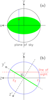 |
Fig. B.1 Sketch of the proposed disk+halo model. a. View of the halo in projection onto the plane of the sky. The y axis is the projection of the disk rotation axis. The circle is the outer border of the spherical halo, while the green ellipse represents the disk. The red point indicates a generic LOS and the blue line is the intersection between the halo and the plane parallel to the disk axis and containing the given LOS. b. Cut of the disk+halo corresponding to the blue line in panel a. The green line denotes the disk seen edge on and the red line is the LOS indicated by the red dot in panel a. Points z1 and z2 are the intersections with the halo. The y′ axis is rotated by the angle ψ in the x, z plane with respect to the plane of the sky. The observer lies at z = −∞. |
B.2 Line brightness temperature
The observed line brightness temperature of the disk equals the kinetic temperature of the gas attenuated because of the absorption by dust in the halo along the LOS, namely
![Mathematical equation: $\[T_{\mathrm{B}}=T_{\mathrm{K}}(r) \exp [-\tau(x, y)]\]$](/articles/aa/full_html/2025/01/aa52686-24/aa52686-24-eq51.png) (B.5)
(B.5)
with
![Mathematical equation: $\[\tau(x, y)=\int_{z_{1}}^{z_{2}} \kappa_{\mathrm{d}} ~\rho ~\mathrm{d} z\]$](/articles/aa/full_html/2025/01/aa52686-24/aa52686-24-eq52.png) (B.6)
(B.6)
where ![Mathematical equation: $\[r=\sqrt{x^{\prime 2}+y^{\prime 2}}, \kappa_{\mathrm{d}}\]$](/articles/aa/full_html/2025/01/aa52686-24/aa52686-24-eq53.png) is the dust absorption coefficient, ρ the density of the halo, and z1 and z2 the intersections of the LOS with, respectively, the halo and the disk (see Fig. B.1b). For a generic LOS x, y, the latter can be expressed as
is the dust absorption coefficient, ρ the density of the halo, and z1 and z2 the intersections of the LOS with, respectively, the halo and the disk (see Fig. B.1b). For a generic LOS x, y, the latter can be expressed as
![Mathematical equation: $\[z_{1}=-\sqrt{R_{\mathrm{d}}^{2}-x^{2}-y^{2}}\]$](/articles/aa/full_html/2025/01/aa52686-24/aa52686-24-eq54.png) (B.7)
(B.7)
![Mathematical equation: $\[z_{2}=y ~\tan~ \psi.\]$](/articles/aa/full_html/2025/01/aa52686-24/aa52686-24-eq55.png) (B.8)
(B.8)
We note that ![Mathematical equation: $\[\sqrt{R_{\mathrm{d}}^{2}-x^{2}}\]$](/articles/aa/full_html/2025/01/aa52686-24/aa52686-24-eq56.png) is the radius of the circle that corresponds to the intersection between the halo and the plane containing the LOS and parallel to the disk axis (blue circle in Fig. B.1b).
is the radius of the circle that corresponds to the intersection between the halo and the plane containing the LOS and parallel to the disk axis (blue circle in Fig. B.1b).
Under the assumption that the density of the halo scales like ρ = ρ0(Rd/R) with ![Mathematical equation: $\[R=\sqrt{x^{2}+y^{2}+z^{2}}\]$](/articles/aa/full_html/2025/01/aa52686-24/aa52686-24-eq57.png) distance of a point of the halo from the center, Eq. (B.6) can be written as
distance of a point of the halo from the center, Eq. (B.6) can be written as
![Mathematical equation: $\[\begin{aligned}\tau(x, y) & =\kappa_{\mathrm{d}} ~\rho_0 ~R_{\mathrm{d}} \int_{z_1}^{z_2} R^{-1} \mathrm{~d} z \\& =\tau_0 \ln \left(\frac{y ~\tan~ \psi+\sqrt{x^2+y^2\left(1+\tan ^2 \psi\right)}}{R_{\mathrm{d}}-\sqrt{R_{\mathrm{d}}^2-x^2-y^2}}\right)\end{aligned}\]$](/articles/aa/full_html/2025/01/aa52686-24/aa52686-24-eq58.png) (B.9)
(B.9)
where τ0 ≡ κd ρ0 Rd is a dimensionless free parameter of the model.
Finally, TK can be expressed as a function of x and y from Eqs. (3) and (B.2):
![Mathematical equation: $\[T_{\mathrm{K}}(\mathrm{K})=158\left[\frac{x^{2}+\left(\frac{y}{\cos~ \psi}\right)^{2}}{R_{\mathrm{d}}^{2}}\right]^{-0.16}.\]$](/articles/aa/full_html/2025/01/aa52686-24/aa52686-24-eq59.png) (B.10)
(B.10)
For our calculations, we have assumed a disk radius ![Mathematical equation: $\[R_{\mathrm{d}}{=}0^{\prime\prime}_\cdot3{=}490\]$](/articles/aa/full_html/2025/01/aa52686-24/aa52686-24-eq60.png) au, estimated from the maximum size of the distribution of the CH3CN peaks in Fig. 15a.
au, estimated from the maximum size of the distribution of the CH3CN peaks in Fig. 15a.
In conclusion, the measured TB along a given LOS x, y crossing the disk can be computed by substituting Eqs. (B.9) and (B.10) into Eq. (B.5), while x, y are related to the position in right ascension and declination through Eqs. (B.3) and (B.4).
References
- Andrews, 2020, ARA&A, 58, 483 [NASA ADS] [CrossRef] [Google Scholar]
- Bayandina, O. S., Moscadelli, L., Cesaroni, R., et al. 2024, A&A, submitted [Google Scholar]
- Benisty, M., Dominik, C., Follette, K., et al. 2023, in Protostars and Planets VII, eds. S. Inutsuka, Y. Aikawa, T. Muto, K. Tomida, & M. Tamura (Astronomical Society of the Pacific Conference Series), 605 [Google Scholar]
- Caratti o Garatti, A., Froebrich, D., Eislöffel, J., Giannini, T., & Nisini, B. 2008, A&A, 485, 137 [NASA ADS] [CrossRef] [EDP Sciences] [Google Scholar]
- Cesaroni, R., Felli M., Testi L., Walmsley C.M., & Olmi L. 1997, A&A, 325, 725 [NASA ADS] [Google Scholar]
- Cesaroni, R., Felli, M., Jenness, T., et al. 1999, A&A, 345, 949 [NASA ADS] [Google Scholar]
- Cesaroni, R., Neri, R., Olmi, L., et al. 2005, A&A, 434, 1039 [NASA ADS] [CrossRef] [EDP Sciences] [Google Scholar]
- Cesaroni, R., Beltrán, M.T., Zhang, Q., Beuther, H., & Fallscheer, C. 2011, A&A, 533, A73 [NASA ADS] [CrossRef] [EDP Sciences] [Google Scholar]
- Cesaroni, R., Massi, F., Arcidiacono, C., et al. 2013, A&A, 549, A146 [NASA ADS] [CrossRef] [EDP Sciences] [Google Scholar]
- Cesaroni R., Galli D., Neri R., & Walmsley C. M. 2014, A&A, 566, A73 [NASA ADS] [CrossRef] [EDP Sciences] [Google Scholar]
- Cesaroni, R., Faustini, F., Galli, D., et al. 2023, A&A, 671, A126 [NASA ADS] [CrossRef] [EDP Sciences] [Google Scholar]
- Chen, H.-R. V., Keto, E., Zhang, Q., et al. 2016, ApJ, 823, 125 [NASA ADS] [CrossRef] [Google Scholar]
- Garufi, A., Benisty, M., Pinilla, P., et al. 2018, A&A, 620, A94 [NASA ADS] [CrossRef] [EDP Sciences] [Google Scholar]
- Hirota, T., Nagayama, T., Honma, M., et al. 2020, PASJ, 72, 50 [NASA ADS] [CrossRef] [Google Scholar]
- Hofner, P., Cesaroni, R., Rodríguez, L. F., & Martí, J. 1999, A&A, 345, L43 [NASA ADS] [Google Scholar]
- Hofner, P., Cesaroni, R., Olmi, L., et al. 2007, A&A, 465, 197 [NASA ADS] [CrossRef] [EDP Sciences] [Google Scholar]
- Johnston, K. G., Keto, E., Robitaille, T. P., & Wood, K. 2011, MNRAS, 415, 2953 [NASA ADS] [CrossRef] [Google Scholar]
- Kawamura, J. H., Hunter, T. R., Tong, C.-Y. E., et al. 1999, PASP, 111, 1088 [CrossRef] [Google Scholar]
- Keto, E., & Zhang, Q. 2010, MNRAS, 406, 102 [NASA ADS] [CrossRef] [Google Scholar]
- Kurtz, S., Cesaroni, R., Churchwell, E., Hofner, P., & Walmsley, C.M. 2000, in Protostars and Planets IV, eds. V. Mannings, A. Boss, S. Russel [Google Scholar]
- Massi, F., Caratti o Garatti, A., Cesaroni, R., et al. 2023, A&A, 672, A113 [NASA ADS] [CrossRef] [EDP Sciences] [Google Scholar]
- Montes, V. A., Hofner, P., Anderson, C., & Rosero, V. 2015, ApJS, 219, 41 [NASA ADS] [CrossRef] [Google Scholar]
- Moscadelli, L., Cesaroni, R., & Rioja, M. J. 2005, A&A, 438, 889 [NASA ADS] [CrossRef] [EDP Sciences] [Google Scholar]
- Moscadelli, L., Cesaroni, R., Rioja, M. J., Dodson, R., & Reid, M. J. 2011, A&A 526, A66 [NASA ADS] [CrossRef] [EDP Sciences] [Google Scholar]
- Palau, A., Walsh, C., Sánchez-Monge, Á., et al. 2017, MNRAS, 467, 2723 [NASA ADS] [Google Scholar]
- Qiu, K., Zhang, Q., Megeath, S. Th., et al. 2008, ApJ, 685, 1005 [NASA ADS] [CrossRef] [Google Scholar]
- Sánchez-Monge, Á., Cesaroni, R., Beltrán, M. T., et al. 2013, A&A, 552, L10 [NASA ADS] [CrossRef] [EDP Sciences] [Google Scholar]
- Sánchez-Monge, Á., Schilke, P., Ginzburg, A., Cesaroni, R., & Schmiedeke, A. 2018, A&A, 609, A101 [NASA ADS] [CrossRef] [EDP Sciences] [Google Scholar]
- Shepherd, D. S., Yu, K. C., Bally, J., & Testi, L. 2000, ApJ, 535, 833 [Google Scholar]
- Su, Y.-N., Liu, S.-Y., Chen, H.-R., Zhang, Q., & Cesaroni, R. 2007, ApJ, 671, 571 [NASA ADS] [CrossRef] [Google Scholar]
- Toomre, A. 1964, ApJ, 139, 1217 [Google Scholar]
- Walmsley, C. M. 1995, in Rev. Mexicana Astron. Astrofis. Ser. Conf., 1, Circumstellar Disks, Outflows, and Star Formation, eds. S. Lizano, & J. M. Torrelles (Mexico, DF: Inst. Astron., UNAM), 137 [Google Scholar]
- Wilking, B. A., Blackwell, J. H., & Mundy, L. G. 1990, AJ, 100, 758 [NASA ADS] [CrossRef] [Google Scholar]
CASA can be downloaded from http://casa.nrao.edu
The GILDAS software has been developed at IRAM and Observatoire de Grenoble and is available at http://iram.fr/IRAMFR/GILDAS/
The so-called moment-8 maps are obtained by selecting the maximum intensity across the spectrum for each pixel of the image. With respect to the maps obtained by averaging the line emission over a broad velocity range, the moment-8 maps have the advantage of also being sensitive to faint, narrow lines.
All Figures
|
Fig. 1 Moment-8 maps in various molecular tracers of the jet in IRAS 20126+4104. All maps have been rotated by 30° clockwise so that the jet axis lies parallel to the X-axis of the plot. The offset is relative to the phase center of the observations. The ellipse in the bottom left corner indicates the synthesized beam of the ALMA maps. (a) Contour map of the SiO(5–4) line emission overlaid on the image of the H2 2.12 μm line obtained by Cesaroni et al. (2013). Contour levels range from 10.4 to 136.4 in steps of 21 mJy/beam. (b) Contour map of the H2CO (30,3–20,2) line emission overlaid on the same SiO(5–4) image as in panel a. Contour levels range from 27 to 117 in steps of 15 mJy/beam. (c) Same as panel b but for the contour map of the average emission in the H2CO (32,2–22,1) and (32,1–22,0) lines. Contour levels range from 12 to 111 in steps of 9 mJy/beam. (d) Same as panel b but for the contour map of the CH3OH (4−2,3–3−1,2) E line emission. Contour levels range from 16.2 to 111.2 in steps of 19 mJy/beam. |
| In the text | |
|
Fig. 2 Normalized intensity profile along the jet axis. The X-axis is the same as in Fig. 1 but spans only the range of angles corresponding to the NW lobe of the jet. The meaning of the different curves is given in the figure. |
| In the text | |
|
Fig. 3 Moment-8 PV diagrams in three molecular tracers of the jet along the direction with a PA of −60°. The offset is relative to the phase center of the observations. The cross in the bottom left corner indicates the angular and spectral resolutions. (a) Contour map of the H2CO (30,3–20,2) line emission overlaid on the SiO(5–4) map. Contour levels range from 22 to 112 in steps of 15 mJy/beam. (b) Same as panel a but for the contour map of the CH3OH (4−2,3–3−1,2) E line emission. Contour levels range from 16.2 to 111.2 in steps of 19 mJy/beam. |
| In the text | |
|
Fig. 4 Map of the 1.4 mm continuum emission (contours) overlaid on the moment-8 map of the CH3CN(12–11) K=3 (panel a) and 13CH3CN(13–12) K=3 line (panel b). Contour levels range from 1.4 to 26.6 in steps of 2.8 mJy/beam. The ellipses in the bottom left and right corners indicate the synthesized beam of the continuum and line maps, respectively. |
| In the text | |
|
Fig. 5 Moment-9 maps of the CH3CN(12–11) K=3 (panel a) and 13CH3CN(13–12) K=3 (panel b) lines. The systemic velocity is ~−3.9 km s−1. The solid line shows the deconvolved direction of the major axis of the continuum emission, while the dashed lines give the errors on this direction. The blue and red arrows indicate the directions of the blue- and redshifted lobes of the jet shown in Fig. 1. The ellipses in the bottom right corners denote the synthesized beams. |
| In the text | |
|
Fig. 6 SiO(5–4) line emission in IRAS 20126+4104. The offsets are relative to the phase center of the observations. (a) Moment-8 map of the emission rotated by 30° clockwise, so that the jet axis lies parallel to the X-axis of the plot. The dotted lines indicate the cuts used to make the PV diagrams in panels c and d. According to our conical jet model, emission can be seen only in the region comprised between the two dashed lines. The horizontal and vertical lines mark the position of the 1.4 mm continuum peak. (b) Moment-8 PV diagram along the jet axis. The dotted lines have the same meaning as in panel a. The cross in the bottom left corner indicates the angular and spectral resolutions. The vertical line marks the position of the continuum peak and the horizontal line the systemic velocity of −3.9 km s−1. (c) PV diagram along the dotted line at offset |
| In the text | |
|
Fig. 7 Contour map of the SiO emission (same as in Fig. 1a) overlaid on maps of the H2CO rotational temperature (panel a) and column density (panel b). The maps have been rotated by 30° clockwise. The ellipse in the bottom right corner denotes the synthesized beam. The cross marks the position of the 1.4 mm continuum peak. |
| In the text | |
|
Fig. 8 Moment-8 PV diagrams of various molecular transitions along the disk plane (PA=53°). The offset is relative to the phase center of the observations. The horizontal and vertical lines mark the systemic velocity and the position of the 1.4 mm continuum peak, respectively. The crosses in the bottom left corners indicate the angular and spectral resolutions. (a) PV plot of the CH3CN(12–11) K=3 component (contours) overlaid on that of the DCN(3–2) line. Contour levels range from 7 to 91 in steps of 12 mJy/beam. (b) Same as panel a, with CH3CN(12–11) K=7 overlaid on K=3. Contour levels range from 5 to 53 in steps of 6 mJ /beam. (c) Same as panel a, but with |
| In the text | |
|
Fig. 9 Distribution of the peaks (colored points) obtained by fitting a 2D Guassian to the emission in each channel of the channel maps of the CH3CN(12–11) K=3 line. The colored ellipses are the deconvolved FWHM of the fitted Gaussians. The color corresponds to the LSR velocity as indicated by the scale to the right. The black cross and ellipse represent the peak position and deconvolved FWHM of the 1.4 mm continuum emission, respectively. The dashed line outlines the direction of the major axis of the black ellipse. The shaded ellipse in the bottom right corner represents the synthesized beam. |
| In the text | |
|
Fig. 10 Absolute value of the angle between the major axis of the deconvolved FWHM of the emission in the line channel, and the axis of the disk versus the LSR velocity of the channel. The colors correspond to the CH3CN(12–11) lines as indicated in the figure. The vertical line marks the systemic velocity. The horizontal line corresponds to |Θ| = 90°. |
| In the text | |
|
Fig. 11 Schematic plot of the velocity along the line of sight relative to the star velocity, in a template Keplerian disk inclined by 30°. The plane of the figure is the plane of the sky and the dashed line is the projection of the disk rotation axis. The color scale indicating the velocity is in arbitrary units. We note that the high-velocity magenta/red and blue patterns are elongated perpendicular to the yellow/green patterns, which correspond to velocities close to zero. |
| In the text | |
|
Fig. 12 Moment-8 PV diagram of the DCN(3–2) line emission along the plane of the disk (PA=53°). The offset is relative to the phase center of the observations. The black and white points mark the emission peaks obtained by fitting a Gaussian to the emission, respectively, for fixed offset and fixed velocity. The solid squares indicate the points selected by us to define the velocity–radius relation in the Keplerian disk. |
| In the text | |
|
Fig. 13 Analysis of the temperature and column density distribution in the disk around IRAS 20126+4104. (a) PV diagram along the disk plane of the CH3CN rotation temperature obtained by fitting the brightness temperature of selected transitions. The black solid squares mark the points used to derive Trot as a function of radius (see text). (b) Same as panel a but for the CH3CN column density. (c) Rotation temperature versus angular radius obtained from the points of the PV diagram marked by the black solid squares. The solid line is a linear fit to the data corresponding to the relation Trot(K) = 107 [θ(arcsec)]−0.32. The dashed line corresponds to half the synthesized beam. (d) Same as panel c but for the CH3CN column density. The relationship obtained from the linear fit to the data is Ncol(cm−2) = 1.1 × 10¹⁵ [θ(arcsec)]−1.3. |
| In the text | |
|
Fig. 14 LSR velocity corresponding to the peak emission in the PV diagrams of the CH3CN(12–11) K = 2, 3, 4, 5, 7, 8 lines as a function of the upper energy of the transition. The dashed line marks the systemic LSR velocity of −3.9 km s−1. |
| In the text | |
|
Fig. 15 Distributions of the peaks of the emission in the velocity channels of various lines observed in IRAS 20126+4104. The error bars are the formal errors on the Gaussian fits. The offsets are relative to the phase center of the observations. The black cross marks the position of the 1.4 mm continuum peak. (a) Plot obtained from the CH3CN(12–11) lines. The color coding is as follows: K=2 black, 3 red, 4 green, 5 blue, 7 cyan, 8 yellow, and v8=1 magenta. The dashed lines are linear fits to the points obtained by fitting Y vs X and X vs Y; the solid line is the mean of the two. (b) Same as panel a but for the 13CH3CN(13–12) components: K=2 black, 3 red, 4 green, and 5 blue. (c) Same as panel a but for the |
| In the text | |
|
Fig. 16 Peaks of the CH3CN(12–11) K = 2, 3, 4, 5, 7, 8 components in the different velocity channels overlaid on the best-fit model of a disk undergoing Keplerian rotation and radial infall (see text). The data have been rotated counterclockwise by 42° to align the disk with the X-axis. The offsets are relative to the disk center. The color indicates the velocity along the line of sight relative to the star. The black cross marks the position of the 1.4 mm continuum peak. |
| In the text | |
|
Fig. 17 Maps of the velocity and dust opacity over the disk according to our model. The black ellipse outlines the border of the disk and the color-coded patterns are the loci of points of the disk with the same velocity along the line of sight, ranging from −10 to +10 in steps of 1 km s−1. The gray scale with dotted contours is a map of the envelope dust opacity. |
| In the text | |
|
Fig. 18 Comparison between the peaks of the CH3CN(12–11) K = 2, 3, 4, 5, 7, 8 components in the different velocity channels (solid circles) and those obtained from the model for a template line (empty circles connected by the solid line). We note that the model peak distribution qualitatively reproduces the C-shaped pattern described by the data. The system is rotated clockwise by 42° and the offsets are relative to the phase center of the observations. The color indicates the LSR velocity. The black square marks the center of the disk according to the model. The black cross indicates the position of the 1.4 mm continuum peak with error bars. |
| In the text | |
|
Fig. 19 Overlay of the CH3CN peaks (circles) on the moment-8 map (contours) of the SiO(5–4) line emission. The colored points and black cross are the same as in Fig. 18. The maps have been rotated by 42° counterclockwise for consistency with Fig. 18 and the offsets are relative to the phase center of the observations. The contour levels range from 6 to 36 in steps of 5 mJy/beam. The ellipse in the bottom left corner denotes the synthesized beam of the SiO map. |
| In the text | |
|
Fig. A.1 Sketch of the proposed conical model for the jet. a. View of the jet in projection onto the plane of the sky. We indicate the apparent opening angle with θ′. b. Projection of the jet onto the x, z plane. Here θ is the true opening angle and ϕ the inclination angle of the jet axis with respect to the plane of the sky. The observer lies at z = −∞. The z′ axis coincides with the axis of the cone, while we choose y′ = y. |
| In the text | |
|
Fig. B.1 Sketch of the proposed disk+halo model. a. View of the halo in projection onto the plane of the sky. The y axis is the projection of the disk rotation axis. The circle is the outer border of the spherical halo, while the green ellipse represents the disk. The red point indicates a generic LOS and the blue line is the intersection between the halo and the plane parallel to the disk axis and containing the given LOS. b. Cut of the disk+halo corresponding to the blue line in panel a. The green line denotes the disk seen edge on and the red line is the LOS indicated by the red dot in panel a. Points z1 and z2 are the intersections with the halo. The y′ axis is rotated by the angle ψ in the x, z plane with respect to the plane of the sky. The observer lies at z = −∞. |
| In the text | |
Current usage metrics show cumulative count of Article Views (full-text article views including HTML views, PDF and ePub downloads, according to the available data) and Abstracts Views on Vision4Press platform.
Data correspond to usage on the plateform after 2015. The current usage metrics is available 48-96 hours after online publication and is updated daily on week days.
Initial download of the metrics may take a while.