| Issue |
A&A
Volume 679, November 2023
|
|
|---|---|---|
| Article Number | A3 | |
| Number of page(s) | 18 | |
| Section | The Sun and the Heliosphere | |
| DOI | https://doi.org/10.1051/0004-6361/202347142 | |
| Published online | 30 October 2023 | |
Solar photospheric spectrum microvariability
I. Theoretical searches for proxies of radial-velocity jittering
1
Lund Observatory, Division of Astrophysics, Department of Physics, Lund University, 22100 Lund, Sweden
e-mail: This email address is being protected from spambots. You need JavaScript enabled to view it.
2
Zentrum für Astronomie der Universität Heidelberg, Landessternwarte, Königstuhl, 69117 Heidelberg, Germany
e-mail: This email address is being protected from spambots. You need JavaScript enabled to view it.
Received:
9
June
2023
Accepted:
18
August
2023
Abstract
Context. Extreme precision radial-velocity spectrometers enable extreme precision in stellar spectroscopy. Searches for low-mass exoplanets around solar-type stars are limited by various types of physical variability in stellar spectra, such as the short-term jittering of apparent radial velocities on levels of ∼2 m s−1.
Aims. To understand the physical origins of radial-velocity jittering, the solar spectrum is assembled, as far as possible, from basic principles. Solar surface convection is modeled with time-dependent 3D hydrodynamics, followed by the computation of high-resolution spectra during numerous instances of the simulation sequence. The behavior of different classes of photospheric spectral lines is monitored throughout the simulations to identify commonalities or differences between different classes of lines: weak or strong, neutral or ionized, high or low excitation, atomic or molecular.
Methods. Synthetic spectra were examined. With a wavelength sampling λ/Δλ ∼ 1 000 000, the changing shapes and wavelength shifts of unblended and representative Fe I and Fe II lines were followed during the simulation sequences. The radial-velocity jittering over the small simulation area typically amounts to ±150 m s−1, scaling to ∼2 m s−1 for the full solar disk. Flickering within the G-band region and in photometric indices of the Strömgren uvby system were also measured, and synthetic G-band spectra from magnetic regions are discussed.
Results. Most photospheric lines vary in phase, but with different amplitudes among different classes of lines. Amplitudes of radial-velocity excursions are greater for stronger and for ionized lines, decreasing at longer wavelengths. Matching precisely measured radial velocities to such characteristic patterns should enable us to remove a significant component of the stellar noise originating in granulation.
Conclusions. The granulation-induced amplitudes in full-disk sunlight amount to ∼2 m s−1; the differences between various line groups are an order of magnitude less. To mitigate this jittering, a matched filter must recognize dissimilar lineshifts among classes of diverse spectral lines with a precision of ∼10 cm s−1 for each line group. To verify the modeling toward the filter, predictions of center-to-limb dependences of jittering amplitudes for different classes of lines are presented, testable with spatially resolving solar telescopes connected to existing radial-velocity instruments.
Key words: Sun: photosphere / techniques: radial velocities / Sun: granulation / stars: solar-type / techniques: spectroscopic / line: profiles
© The Authors 2023
 Open Access article, published by EDP Sciences, under the terms of the Creative Commons Attribution License (https://creativecommons.org/licenses/by/4.0), which permits unrestricted use, distribution, and reproduction in any medium, provided the original work is properly cited.
This article is published in open access under the Subscribe to Open model. This email address is being protected from spambots. You need JavaScript enabled to view it. to support open access publication.
1. Introduction
Extreme precision stellar spectroscopy is now enabled at several observatories, using extreme precision radial-velocity spectrometers designed for a wavelength stability corresponding to Doppler shifts of ∼1 m s−1 or less. These instruments are operating at several large and very large telescopes, for example CARMENES on Calar Alto (Quirrenbach et al. 2014, 2018), ESPRESSO at the ESO VLT on Paranal (Pepe et al. 2014, 2021); EXPRES at the Lowell Discovery Telescope in Arizona (Jurgenson et al. 2016; Blackman et al. 2020); HARPS (Mayor et al. 2003; Coffinet et al. 2019) and NIRPS (Bouchy et al. 2017) at ESO on La Silla; HARPS-North and the forthcoming HARPS-3 on La Palma (Cosentino et al. 2012; Thompson et al. 2016), HPF on the Hobby-Eberly Telescope in Texas (Kanodia et al. 2021; Mahadevan et al. 2014); iLocater on LBT in Arizona (Crass et al. 2022); the Keck Planet Finder (KPF) on Maunakea (Gibson et al. 2016); MAROON-X at Gemini-North on Maunakea (Seifahrt et al. 2018, 2022); NEID at WYIN on Kitt Peak (Schwab et al. 2016); SPIRou at CFHT on Maunakea (Donati et al. 2020; Hobson et al. 2021); Veloce Rosso at AAT in Australia (Gilbert et al. 2018); and a few others. These performance requirements are also in the design criteria of future instruments for extremely large telescopes (Halverson et al. 2016; Marconi et al. 2022; Plavchan et al. 2019; Szentgyorgyi et al. 2018).
The primary task for these spectrometers is to search for periodic modulations of stellar radial velocities induced by orbiting exoplanets. The detection of planets with successively lower mass requires recognizing successively smaller velocity amplitudes. For an Earth-mass planet orbiting a solar-mass star in a one-year orbit, the expected signal amounts at most to only 0.1 m s−1 (e.g., Hall et al. 2018). The precision of current and foreseen instruments is now actually beginning to approach these levels, soon enabling such very challenging observations. However, radial-velocity fluctuations of much greater amplitude are contributed by stellar phenomena, such as convective motions in granulation and supergranulation, p-mode oscillations, modulation by dark starspots and bright magnetically active regions carried in and out of sight by stellar rotation, changes in surface structure during long-term magnetic activity cycles, among others. The requirement of mitigating effects of stellar activity for radial-velocity measurements was realized long ago (e.g., Dravins 1989), and to segregate these often irregular effects from the more regular modulation induced by planets, comprehensive data analysis methods have been developed to scrutinize spectra recorded with current instruments. These typically include the calculation of cross-correlation or other statistical functions to find the wavelength displacement relative to a template, with various adjustments applied using the asymmetries or widths of these functions. The level of magnetic activity can be estimated from simultaneously measured chromospheric emission, usually in the cores of the Ca II H & K-lines, but also feasible from statistics of Zeeman broadening (Lienhard et al. 2023). Extensive comparisons between different methods advocated by different groups have been carried out, testing software routines on data with both a synthetic planetary signal injected, and for sequences of pure stellar observations (Dumusque 2016; Dumusque et al. 2017; Hara & Ford 2023; Zhao et al. 2022).
While such routines do succeed in eliminating much of the nonplanetary signals, even the current best modeling of stellar variability is unable to extract planetary signals with amplitudes much less than 1 or 2 m s−1. The limitations are thus no longer instrumental or technical, but lie in understanding the complexities of atmospheric dynamics and spectral line formation, revealed as a jitter of the apparent radial velocity and a flickering of the photometric irradiance. As concluded in reviews of the field (Fischer et al. 2016), and in reports from working groups for precision radial velocities and exoplanet detection (Crass et al. 2021; Rackham et al. 2023), some significantly different approaches will be required in order to reach precisions of 10 cm s−1 or better, as ultimately required to find an exoEarth.
The aim of this paper is not to further refine methods in analyzing observed spectra, but instead to start to try to understand the physical origins of radial-velocity jittering in solar and stellar atmospheres. To reach challenging goals of precisions in the cm s−1 range, it will probably not be sufficient to apply statistical analyses on observed data, but it will be necessary to somehow exploit the information content of the many thousands of different spectral lines in solar-type stars.
We examined the time sequences of synthetic solar spectra, as computed from hydrodynamic simulations of the solar photosphere. In principle, this amounts to watching movies of high-resolution solar spectral atlases and searching for systematic patterns of variability, in particular those that correlate with excursions in apparent radial velocity.
The paper is organized as follows. Section 2 describes the background, the aims, and the prerequisites of our method, and places the velocity jittering over the simulation areas in the context of the full solar disk. Section 3 describes how the overall synthetic spectra are obtained, and Sect. 4 how the properties of their individual spectral lines are measured. Section 5 analyzes the wavelength jittering of groups of selected Fe I and Fe II lines. Section 6 examines the behavior of the molecular G-band and surrounding atomic lines, including a discussion of their formation physics and effects by magnetic fields. Section 7 evaluates the fluctuations in color indices from broader band uvby Strömgren photometry. Section 8 documents searches for the spectral-line parameters that failed to yield significant correlations with excursions in radial velocity. The conclusion is presented in Sect. 9, and outlines how it should be possible to diminish the jittering signal arising from surface convection in searches for low-mass exoplanets. The subsequent Paper II (Dravins & Ludwig, in prep.) will evaluate signatures of microvariabilty in observations of the Sun seen as a star, also guided by the conclusions from this Paper I.
2. Synthesizing spectra from line formation physics
A huge amount of work has been done in analyzing and dissecting observed spectra, using a multitude of statistical and other functions, but appears to have hit a boundary at the m s−1 level. Instead of scrutinizing observed spectra from the top down, we tried to assemble and construct not-yet-observed stellar spectra from the bottom up, as far as possible from basic principles. By numerically simulating the stellar atmospheric structure and dynamics ab initio for both quiet and magnetically active regions, and knowing the physical conditions in the model, signatures from dynamic stellar surface inhomogeneities can be traced forward into the complete synthetic spectrum. Different classes of stellar surface features (hot or cold, magnetic or not) affect different classes of spectral lines (weak or strong, neutral or ionized, high or low excitation, atomic or molecular) to varying degrees, and it should also be possible to identify and calibrate their effects in the spectrum of the full stellar disk.
This approach is made feasible by two developments. First, on the theoretical side, convectively driven gas motion near stellar surfaces can now be modeled in detail with time-dependent 3D (magneto-)hydrodynamics, and these simulations are now established as quite realistic descriptions of the spectral-line forming regions in the photospheres of at least solar-type stars. A more recent development is the computation of complete stellar spectra from such models (Chiavassa et al. 2018; Dravins et al. 2021a,b; Ludwig et al., in prep.). These models produce complete and complex stellar spectra, incorporating a huge number of spectral lines from databases such as VALD1 (Heiter et al. 2015; Ryabchikova et al. 2015), and are able to so do so in sampling wavelengths with a hyper-high spectral resolution (λ/Δλ ∼ 1 000 000)2, spanning all observable spectral ranges. Details in the resulting spectra depend on a complex interplay between, for example, atmospheric opacity in different atmospheric inhomogeneities, blending of multiple spectral lines, and the different viewing angles across the stellar disk in different wavelength regions. The modeling entails various approximations, but since the synthetic spectra are free from random photometric noise, spectral microvariability such as the radial-velocity jittering of different spectral features can be followed throughout the simulation sequences by measuring the relative wavelength displacements of any feature anywhere in the spectrum and correlations with other spectral parameters identified.
2.1. Photometric irradiance flickering
Corresponding challenges in microvariability exist for the photometric flickering, a limiting parameter in identifying photometric transits of small planets across stellar disks and also, more generally, a diagnostic tool for studying the presence of granulation on stellar surfaces as predicted from hydrodynamic models for different classes of stars (e.g., Ludwig 2006; Lundkvist et al. 2021). With ∼106 granules across the solar disk, typical brightness contrasts of ∼20% in each granule reduces to ∼2 × 10⁻⁴ after averaging over a million random locations (e.g., Nèmec et al. 2020). Precision photometry from space reveals the temporal power spectra of the flickering, and can be used to infer stellar properties (Cranmer et al. 2014; Kallinger et al. 2014; Samadi et al. 2013a,b; Sulis et al. 2020).
2.2. Limitations of theory
Ideally, we could envision detailed magnetohydrodynamic simulations embracing entire stellar surfaces, producing time-variable spectral atlases for varying mixtures of different types of surface structures on different classes of stars. This is not yet practical and the scope has to be limited. We start with the solar spectrum, both because it is the most studied and modeled one, and because theoretical predictions can be observationally tested in great detail. Realistic 3D simulation volumes can cover groups of multiple photospheric granules and permit us to follow how their appearance changes when seen under different angles, from disk center out toward the limb. Even so, simulated solar surface areas can cover only a small fraction of the full surface.
As described in Sect. 5 below, the equivalent of a full solar disk is obtained from this simulation area of 5.6 × 5.6 Mm2 by summing appropriately weighted spectra from various computed center-to-limb angles, producing a spectrum that retains the fluctuations from the small simulation area. The actual solar hemisphere area is larger by a factor of ∼100 000, and the projected solar disk by ∼50 000. In the case of statistically independent random fluctuations (neglecting details of geometric projection effects and statistical weighting by limb darkening), the averaged full-disk amplitudes should then decrease by a factor equal to the square root of this number. However, away from disk center, spectra are also computed for up to eight different azimuthal directions, thus providing some further averaging. Nevertheless, even if such spectra are dissimilar, as seen from various oblique directions, the samples are from the same instance in time and cannot be considered statistically fully independent. While it is difficult to precisely quantify their level of randomness, the amplitudes for the actual full solar disk can be expected to average out to ∼150−200 times smaller than those from our modest simulation volume. As we show below, the jittering of spectral lines averaged over the simulation area typically extend over ∼300 m s−1, which would then reduce to ∼1−2 m s−1 in actual integrated sunlight, which are the magnitudes of microvariability to be studied here.
The modeling discussed in this first paper deals mainly with nonmagnetic granulation. This covers most of the solar surface, and provides most of the solar flux. Analyses of the time-variable spectra from the simulation volume enable us to identify relations between various parameters and to extrapolate what amounts should remain in actual full-disk spectra. However, to properly reproduce larger-scale features such as supergranular flows or p-mode oscillations will require (much) larger simulation volumes. In addition, a significant part of the spectrum variability originates in regions of magnetic granulation and spots. Magnetohydrodynamic 3D simulations for these are available and their synthetic spectra can be computed. We postpone this discussion to future papers.
Irrespective of the computational sophistication, the accuracy of synthetic spectra is ultimately limited by the quality of atomic and molecular data. Current synthetic spectra include more than half a million spectral lines; their wavelengths and oscillator strengths originate from laboratory measurements or theoretical predictions. The accuracy of these data, originating from a mixed variety of sources, is somewhat variable. While the overall spectrum does reproduce the observed spectrum to a rather high degree, detailed examination often reveals certain differences concerning relative line strengths and blending lines. For some studies, these limitations may be circumvented; for example, to gain knowledge of the absolute amount of convective blueshifts, an identical spectral synthesis can be repeated with the same input data, but for a static model atmosphere where convective lineshifts cannot exist, and the difference with the hydrodynamic case can then be evaluated (Dravins et al. 2021a). In an analogous vein, we do not need to precisely reproduce the exact strength of each individual spectral feature; instead, we can examine the temporal jittering in wavelength and changes in shapes and strengths of representative types of lines, even if their absolute wavelengths or exact oscillator strengths are not precisely known.
2.3. Realistic project aims
If microvariability signatures generated in stellar atmospheres can be adequately understood, we could then determine what observational efforts would be required to detect and calibrate them. Another motivation for the theoretical and observational aspects is that both are expected to improve in the near future. With enhanced computational capacity, numerical simulations are being extended to greater solar and stellar volumes, also incorporating an increased variety of magnetic features, including sunspot umbrae and penumbrae. Observationally, several light feeds from solar telescopes are now connected to extreme-precision radial velocity spectrometers and are expected to continue collecting data over at least one solar activity cycle or longer. Of additional interest is data from across a spatially slightly resolved solar disk, measured with comparable precision, for example monitoring the characteristics in wavelength jittering in quiet areas versus magnetic ones. This behavior can be theoretically predicted, but the corresponding observations are not yet available, although projects are in progress (Leite et al. 2022).
The variability of the optical spectrum of the Sun seen as a star has previously been studied mainly in features such as Ca II H & K or Hα, but signals in such chromospheric lines are unlikely to precisely relate to radial velocities where the signal comes from photospheric lines alone. However, the number of photospheric features that can potentially be examined, combined, or correlated with one another is enormous, and here only a limited number of selected samples can be surveyed. Our aim is to outline possible paths toward the identification of spectral signatures to serve as proxies for calibrating (at least part of) the radial-velocity jittering in sunlight, and eventually also for other stars. Such proxies would need to be measurable at ground-based observatories independently of the overall radial velocity. These might include velocity differences between various line groups, changes in line depths or widths, or perhaps even broadband photometric colors. A typical photospheric absorption line subtends a wavelength width of ∼10 km s−1, and a radial velocity signal of 1 m s−1 thus amounts to only 1 part in 10 000. Quite possibly, proxies for such signals are comparably minute and may require extensive modeling to be securely identified.
The value of understanding photospheric spectrum microvariability also extends to areas outside monitoring stellar radial motion, such as searches for varying fundamental constants in nature and using precise differences of spectral-line wavelengths in solar-type stars (Berke et al. 2023a,b; Murphy et al. 2022).
3. CO 5BOLD modeling of the solar spectrum
Building upon previous work (Dravins et al. 2017a,b, 2018, 2021a,b), we computed profiles of synthetic spectral lines from 3D atmospheric structures produced in hydrodynamic simulations, using them as grids of space- and time-varying model atmospheres. Two different nonmagnetic solar models were used here: N58 and N59 (Table 1). They both have solar temperature, surface gravity, and metallicity, but differ in some computational aspects, and the details of their granular evolution geometries are somewhat different (although statistically similar). Computationally, the N59 model is a successor to N58, which was examined in Dravins et al. (2021a,b). For example, while the radiation balance in N58 was calculated using five wavelength bins, N59 uses 12, and hence the photospheric energy budget should be better represented. For each model the horizontal simulation area is 5.6 × 5.6 Mm2; each modeling pixel in the 140 × 140 grid of hydrodynamic simulation is equal to 40 × 40 km2 (Table 1). In the simulation sequences, the gradual evolution of granular structures can be followed. Their duration of about two solar hours permitted some 20 temporal snapshots to be selected sufficiently far apart in time to ensure largely uncorrelated granulation flow patterns between successive samples. For these snapshots the spectra for all different elevation and azimuth angles were computed on a grid of 47 × 47 points (each horizontally 120 × 120 km2), downsampled by merging 3 × 3 pixels in the hydrodynamic simulation. Since successive snapshots were chosen well apart in time, their averaging should have a largely random character, but for a given snapshot the spectra at different emerging angles originate from the same granular structures (viewed from different directions), making their level of mutual randomness more difficult to estimate. Details about the computation of these types of models are in Tremblay et al. (2013), where representative synthetic granulation images are also shown, for models at solar temperature and others. Further details are in Ludwig et al. (in prep.).
Identifiers for the CO 5BOLD models used to compute synthetic solar spectra.
From the N58 model, profiles of single, idealized, and isolated spectral lines for Fe I at λ620 nm were computed for five different line strengths and three different lower excitation potentials, χ = 1, 3, and 5 eV. Four different center-to-limb positions μ = cos θ = 1.00, 0.87, 0.59, 0.21, and four azimuth angles ψ = 0, 90°, 180°, and 270° were treated in spectral line synthesis carried out in local thermodynamic equilibrium (LTE). These calculations were made for 19 temporally sampled snapshots during the extent of the simulation. Each profile was computed for 201 wavelength points covering ±15 km s−1. The sampling stepsize thus corresponds to a hyper-high spectral resolution λ/Δλ = 2 000 000. Hyper-high resolution is required to fully resolve intrinsic line asymmetries and to resolve wavelength shifts on levels of cm s−1. Spectra from this series have been discussed in Dravins et al. (2017a,b, 2018), and also in Dravins et al. (2021b).
For the N59 model, complete and complex spectra were computed, incorporating practically all the relevant spectral lines from databases such as VALD. Calculations were made for the spectral range of 120−1000 nm, and for 20 largely uncorrelated instances in time during the simulation. The wavelength sampling corresponds to the hyper-high value λ/Δλ ∼ 900 000. For each instance in time, four center-to-limb angles μ = 1.0, 0.79, 0.41, and 0.09 are provided. The spectra were computed for a total of 21 emergent directions: eight azimuth angles in steps of 45° for μ = 0.79 and 0.41, and four angles in steps of 90° for μ = 0.09. With intensities in absolute units, it becomes possible to also obtain synthetic broadband colors. Time-averaged spectra from analogous types of calculations were presented previously in Dravins et al. (2021a,b) for different classes of stars, but now the spectra are time-resolved.
Despite the spatial averaging over the model area, the total volume of these data is significant: with approximately three million data points in each spectral realization, and for each of the 21 position angles, at each of the 20 instances in time, the total amounts to more than one billion spectral intensity values, requiring some selectivity in the handling of spectra and in choosing and limiting lines for analysis. In the figures the plots for specific center-to-limb positions refer to averages over all computed azimuth angles, unless noted otherwise. Integrated sunlight is computed as for a full disk (and labeled thus in the figures) by appropriately interpolating and summing spectra from different μ-values (Fig. 1). The numerical values, however, refer to those obtained from the small simulation area while, as discussed above, those for the actual Sun are estimated to be smaller by a factor of ∼150−200. Further degrees of freedom are offered by stellar rotational broadening; these variants were treated in Dravins et al. (2017a,b), but here we limit ourselves to rotationally unbroadened lines.
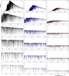 |
Fig. 1. Synthetic solar spectra from the CO 5BOLD N59 model simulation, centered on 525 nm. The spectra are seen over gradually narrower wavelength ranges, decreasing by a factor of 3 for each row from top down. Left column: disk center: μ = cos θ = 1; middle: μ = 0.41; right: μ = 0.09. The intensity scale is common for all frames, and illustrates how the limb darkening is more pronounced at shorter wavelengths. |
Each of the N58 and N59 model spectra offers its advantages and limitations. The advantage with idealized single lines in N58 is that they can highlight possible subtle contrasts between lines of only slightly differing strengths or excitation potentials. However, these lines might not represent observational realities, where not all combinations of line parameters are present and often with multiple blending lines in crowded spectra. Complete spectra are instead produced in N59, but require some effort in selecting representative and distinct spectral features. With more than 600 000 lines included, any selected line will unavoidably also incorporate some weak blends that might have a different temporal behavior than the main line, thus adding some astrophysical noise. The complete spectra in N59 should illustrate what could be practically measurable, while the idealized lines in N58 should help understand the physical origins of possibly identified relations.
A limitation comes from the circumstance that reliable modeling is for the lower photospheric levels in the atmosphere, while higher chromospheric structures are not treated. Consequently, lines that are (partially) formed in the uppermost photosphere or lower chromosphere cannot be expected to be precisely reproduced. On the one hand, the chromospherically influenced lines, perhaps Na I D, the Mg I triplet, or Balmer lines from hydrogen, are not likely to be used for measuring precision radial velocities. However, we still examine their behavior since their modeling may confirm trends when going to stronger lines formed in higher atmospheric layers and they should follow photospheric events more closely than chromospheric Ca II H & K-line emission.
4. Synthetic spectral lines
Figure 1 shows complete synthetic spectra for three center-to-limb angles from the N59 model: disk center μ = 1, μ = 0.41, and μ = 0.09. These data are from one particular instance in time; however, the differences between successive temporal snapshots or between different azimuth angles are much too small to be visible on this scale. Figure 2 gives an example of the selection of differently strong Fe I lines in one particular wavelength region, while Figs. 3 and 4 illustrate the temporal variability in lines from the N59 and N58 models.
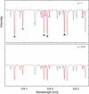 |
Fig. 2. Examples of selected lines. Shown here are Fe I lines around λ525 nm from the N59 model. Top: synthetic spectra at solar disk center, μ = 1; bottom: μ = 0.41. The clean lines selected for detailed analysis are shown in red: strong, medium, and weak labeled A, B, and C, respectively. The lines become noticeably broader toward the limb. |
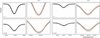 |
Fig. 3. Example of temporal variability of line profiles during the N59 simulation sequence, sampled at 20 instances of time. Left columns: strong Fe Iλ436.59 nm, χ = 2.99 eV line (in the shortward blue); right columns: weak Fe Iλ675.27 nm, χ = 4.64 eV line (in the longward red). The upper row shows profiles for the disk center μ = 1; the bottom row shows integrated sunlight, corresponding to a full solar disk, synthesized using center-to-limb profiles from the small simulation area. The magnified images on the right show the line centers on a uniform wavelength scale in units of radial velocity (top); the tick marks on the vertical axes correspond to those for the full profiles. |
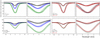 |
Fig. 4. Temporal variability of idealized line profiles during the N58 simulation sequence, sampled at 19 instances of time. Left columns: differently strong Fe I lines at λ620 nm, χ = 3 eV; right columns: lines of similar strength, but with different lower excitation potentials, χ = 1 eV (black) and 5 eV (red). Top row: profiles at disk center μ = 1; bottom row: μ = 0.59. To limit cluttering, profiles are shown for only two (orthogonal) azimuth angles. The right frames show zoomed-in images of the line centers, with wavelength scales equal to those in Fig. 3; the tick marks on the vertical axes correspond to those for the full profiles. |
4.1. Fitting line parameters
To enable searches for dependences among various line parameters, the information resident in the line profiles must somehow be parameterized. We note that the line profiles from each instant in time are not the spatially resolved ones. Such local profiles, originating from specific granular inhomogeneities, display highly varying shapes (e.g., Asplund 2005; Bergemann et al. 2019; Dravins & Nordlund 1990), and (even disregarding the data quantity) would not lend themselves to easily understandable quantification. Each of the current temporally resolved line profiles was spatially averaged over more than 2000 spatial points across the hydrodynamically modeled stellar surface, embracing numerous granulation structures, thereafter resulting in profiles that are closely reminiscent of the temporally averaged profiles, and that can be described with commonly used parameters. However, they still retain noticeable variability over time since the simulation area is tiny compared to the full solar disk.
To quantify these profiles, various tests of line-fitting parameters were made, finding a suitable approximation by fitting with five-parameter Gaussian-type functions of the type y0 − a ⋅ exp[−0.5 ⋅ (|x − x0|/W)c], yielding y0 for the continuum level, a for the line’s absorption depth, W as a measure of the line width, c for the degree of the line’s boxiness or pointedness, and x0 for the central wavelength.
Although the profiles are not precisely Gaussian, these functions appear reliable to use. Different varieties were tested (e.g., Lorentzian), but it was found that such Gaussian-type functions gave robust estimates for all basic line parameters. For the wavelength positions this fitting thus provides one value that refers to the displacement of the line as a whole. For asymmetric profiles, a single number for the line wavelength is not a uniquely defined measure, but depends on whether the fit is made to the central or more extended parts of the profile, and with what type of weighting. However, the physical variability among our line profiles is much greater than possible ambiguities stemming from the exact shape of the fitting functions, and in any case here our aim is not determining absolute line quantities as in Dravins et al. (2021a), but only their relative changes in time. Figure 5 gives a representative example of such a fit.
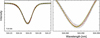 |
Fig. 5. Example of a five-parameter Gaussian-type fit to a typical Fe I line profile in integrated sunlight. Profiles from each temporal snapshot are shown as thin black lines; their average is shown as a dashed red line, and the fitted profile as yellow circles. In the zoomed-in image at the right, the tick marks of the vertical scale correspond to those in the left frame. |
With a significantly greater sample (producing more stable averages), it is also possible to parameterize with respect to line asymmetries or correlations between different portions of the line profile (e.g., Ludwig & Steffen 2008). However, studies of more subtle effects are currently constrained by the limited number of temporal samples. Data from ab initio simulations, where the character of the output cannot be precisely predicted, have a character similar to that of noisy observational data in that they need to be arranged and averaged in order to discern trends. The parameters of wavelength shift and line width appear to be the most readily measurable quantities (also observationally), likewise for the center-to-limb dependences in spatially resolved spectra.
Table 1 gives the unique identifiers of the models, which enables comparisons with other work based on the CO 5BOLD grid (Freytag et al. 2012). The number of sampling points for each spectral line profile is the product of horizontal spatial resolution points in x and y, the number of temporal snapshots extracted during the simulation sequence, and the number of different directions (combined elevation and azimuth angles) for the emerging radiation. The x − y horizontal hsize and z vertical vsize extents of the hydrodynamic simulation volume are given in centimeters.
4.2. Variability in radial velocity and irradiance
Considerable efforts have been made in studying the Sun as a star and in searching for statistical relations between various parameters of solar and stellar variability, including work, and references therein, by Cegla et al. (2019), Collier Cameron et al. (2019, 2021), de Beurs et al. (2022), Dumusque et al. (2015, 2021), Haywood et al. (2016), Lanza et al. (2016, 2019), Maldonado et al. (2019), Marchwinski et al. (2015), and Thompson et al. (2020), and also as reviewed by Hara & Ford (2023). These studies use various statistical approaches to search for possible correlations and empirical proxies for radial-velocity fluctuations. Considerations of other spectral types include Dumusque et al. (2011) and Meunier et al. (2017a,b).
An estimate of the trends in our models indicates that excursions around ±100 m s−1 correspond to about ±1% in irradiance. As discussed above, actual full-disk amplitudes will be reduced from the simulation area by a factor of ∼ 200 or 150, leading to about 0.5 or 0.7 m s−1 per 50 ppm in irradiance. These values seem consistent with those deduced by Cegla et al. (2019), Meunier et al. (2015), and Meunier & Lagrange (2020) for the granulation-induced signal in apparent solar full-disk radial velocity, although further contributions may come from larger-scale structures, such as supergranulation (Meunier & Lagrange 2019), not yet accessible to detailed 3D modeling. A further modeling caution is that brightness variations are also driven by p-mode oscillations which are incompletely treated in the small simulation volumes.
We also note recent related work by Kitiashvili et al. (2023), where synthetic radial-velocity fluctuations are computed from a 3D model of the G0 V star HD 209458, revealing amplitudes of ∼±200 m s−1 over their simulation area of 12.8 Mm width.
5. Photospheric Fe I and Fe II lines
An examination of the simulation sequences shows that different absorption lines generally fluctuate in phase, although with subtle (but systematic) differences between lines of different strength or located in different spectral regions. The absolute amounts of convective blueshift in time-averaged spectra show their familiar dependence on line strength (e.g., Dravins et al. 2021a), but there are also line strength dependences of the amplitudes in the temporal variation of these blueshifts.
To identify systematics in the spectral-line jittering, various correlations were examined between different groups of lines, using the parameters determined from the five-parameter Gaussian-type fitting as described above. From the N58 model, idealized single Fe I lines at λ620 nm were computed with a nominal zero rest wavelength shift, and thus the instantaneous radial velocity value equals the displacement relative to this reference point of zero. Five different line strengths were computed in N58, each for the three different lower excitation potentials of 1, 3, and 5 eV. In all cases the trend of fitted parameters with changing line strengths or excitation potentials was found to be monotonic, and in the following figures only a few representative cases were selected to be plotted.
From the N59 model with complete spectra, groups of clean Fe I lines were selected in representative wavelength regions: around λ430 nm, λ520 nm (Fig. 2), and λ670 nm, and an Fe II sample around λ435 nm. These regions were selected to span different wavelength regions, where lines of different relative strength were also present (labeled strong, medium, and weak). However, the absolute line strengths differ among the regions: Fe I lines in the red are weaker than lines in the blue (Fig. 3), and at longer wavelengths there are too few Fe II lines for a meaningful sample. In addition, a further subdivision in N59 with respect to excitation potential was not seen as practical. The instantaneous radial velocity value for each of these lines is obtained as the displacement relative to each line’s average over the simulation sequence.
The number of temporally separated snapshots during the simulation sequences is 19 for the N58 model and 20 for N59. Each snapshot represents the spatial average over the simulation area, and these are the number of points plotted in the figures below. The values shown are averages for the selected lines from each region; however, it was found that, within each wavelength region, the radial-velocity shifts are almost identical for different lines with the same strength; differences appear only between different line strengths, different wavelength regions, and different excitation potentials. This also implies that the noise in these lineshift plots originates from temporal fluctuations in the granulation structure during the 3D simulation, not photometric or other uncertainties in the computed spectra. To decrease such noise requires spatially and/or temporally more extended simulations.
Figure 6 shows fluctuations in the radial velocities as obtained from fits to isolated, differently strong Fe I lines at λ620 nm in the N58 model; each point indicates a different time during the simulation. For reference, the horizontal axis shows the instantaneous radial velocity for a weak line with the excitation potential 1 eV, while the plot is populated with data points for medium and strong lines, as in Fig. 4. The fitted straight lines confirm that the convective blueshifts systematically decrease with increasing line strength (left panel). There is also a certain dependence on excitation potential (right panel), with higher-excitation lines exhibiting slightly greater blueshifts. However, the trends seen for these idealized lines are less obvious to identify in the real solar spectrum because not many truly high-excitation lines of significant strength exist. These plots are for the solar disk center, μ = 1.
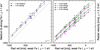 |
Fig. 6. Radial-velocity shifts of synthetic isolated Fe I lines at λ620 nm in the N58 model. Relations between shifts at solar disk center, μ = 1, for weak, medium, and strong lines are shown for different excitation potentials. Each point represents one temporal snapshot during the simulation. The dotted reference lines give the identity relations; the other fitted lines indicate how the dependence of convective blueshift on line strength and excitation potential generally remains valid, even when the spatially averaged radial velocity fluctuates. |
Figure 7 compares differences in instantaneous radial-velocity shifts between pairs of idealized Fe I lines at λ620 nm with modest differences in strength (strong minus medium on the horizontal axis) versus simultaneous differences between more dissimilar lines (strong minus weak on the vertical axis). The plots show systematic trends, such that a given velocity shift between lines of rather similar strengths most often corresponds to a simultaneous but greater shift between lines with greater differences in strength. There, amplitudes between weak and strong lines have some further dependence on excitation potential, although there is scatter among the limited number of data points.
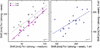 |
Fig. 7. Differences in radial-velocity shifts between lines with different strengths (but similar excitation potentials). These data at μ = 1 are from synthetic isolated Fe I lines at λ620 nm in the N58 model. Each point represents the difference between instantaneous radial velocities (e.g., strong line minus weak) at one temporal snapshot during the simulation. The straight lines are fits to the data points. The different scales between the frames are adapted to reflect how convective blueshifts deviate for lines with increasingly different strengths. |
While Figs. 6 and 7 are for idealized lines at solar disk center, Fig. 8 shows these types of relations for the simulated full solar disk, now measured for essentially unblended lines selected in the complete solar spectrum from the N59 model. The spectrum for the integrated full solar disk is obtained by integrating over a disk, where the spectra from the four computed center-to-limb angles (μ = 1.0, 0.79, 0.41, 0.09) are first averaged over their respective azimuth angles, then interpolated to intermediate center-to-disk positions, and finally summed with appropriate wavelength-dependent limb-darkening values. This is equivalent to the spectrum of a tiny solar disk, where the fluctuation amplitudes of radial velocity, irradiance, and other parameters still refer to the small simulation area. As discussed above, the amplitudes for the actual full solar disk, will be ∼150−200 times smaller, although the exact number is difficult to precisely determine since it depends on understanding the degree to which temporal and azimuthal samples from the simulations can be considered statistically independent.
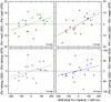 |
Fig. 8. Differences in radial-velocity shifts between Fe I lines of different strengths in different spectral regions of integrated sunlight vs. shifts in medium-strong Fe I lines at λ520 nm. Each point represents one temporal snapshot during the N59 simulation. The spectra correspond to those of a full solar disk, as synthesized from a sequence of center-to-limb spectra, although the numerical values [m s−1] refer to the small simulation area (for the actual Sun, divide by a factor of ∼150−200). The vertical scales differ among the frames. The fitted straight lines suggest the trends, but also indicate the limitation from finite simulation sequences. |
As reference for the radial-velocity, the values for medium-strength lines at λ520 nm (Fig. 2) make up the horizontal axis in Fig. 8. The vertical axes show simultaneous lineshift differences between pairs of line groups with different strengths and/or in various wavelength regions. Despite a scatter of points, all fitted lines indicate qualitatively similar trends; the greatest amplitudes are between strong lines at around λ520 nm and weak lines in the far red at λ670 nm.
Figure 9 summarizes the main trends: velocity jittering in different lines is almost always in phase, but the amplitudes depend on line strength, ionization level, and wavelength region. The greatest amplitudes are noted for Fe II, while for Fe I, both the jittering amplitudes and their differences between differently strong lines decrease for longer wavelengths in the red. These data are from essentially unblended lines selected in the complete solar spectrum from the N59 model. The straight lines at the bottom right show the various fitted trends.
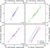 |
Fig. 9. Radial-velocity shifts between Fe I and Fe II lines of relatively similar strengths (strong minus medium) vs. those with greater differences (strong minus weak), in different spectral regions of integrated sunlight. The numerical values refer to the small simulation area in the N59 model (for the actual Sun, divide by a factor of ∼150−200). All frames have identical scales. |
As seen from the horizontal axis of the plot in Fig. 8, the total jittering amplitude over the simulation area is on the order of ±100−200 m s−1, reducing to ∼1−2 m s−1 in integrated sunlight. The difference between weak and strong lines is an order of magnitude smaller (Fig. 9), perhaps ∼0.1−0.2 m s−1, requiring highly precise measurements for detection. However, once these shifts between groups of different spectral lines can be reliably identified, it will constitute a specific signature (for the current discussion, at least of the nonmagnetic granulation), and suitably matched filtering should be able to identify and remove much of that particular atmospheric signature.
5.1. Mechanism of radial-velocity differences
For solar-type stars, the greatest convective blueshifts are found in weak lines formed in the deeper photosphere. However, here we find that the variability of that quantity is smallest in those weak lines and instead increases for stronger lines predominantly formed in the upper photosphere. The mechanism can be tentatively understood by examining a typical 3D atmospheric structure, for example Fig. 14 in Nordlund et al. (2009). That figure shows temperature as a function of optical depth at several horizontal locations across a simulation area. When plotted on an optical-depth scale (not versus geometric height), the temperature dependence on optical depth is similar in hot granules and in cool downflows. The reason is the steep temperature dependence of the opacity, and any given optical depth is reached at about the same temperature, irrespective of whether the temperature gradient is high (as in rising granules) or more modest (as in sinking downflows). Local line strengths, however, depend on the vertical gradients as well.
As illustrated in that figure, the smallest temperature fluctuations occur at optical depths around τ = 0.3, reaching greater but comparable values both deeper down (τ = 1) and higher up, τ = 0.1. Weaker spectral lines form at optical depths of about τ = 0.5, where the fluctuations between various horizontal locations are smaller than those on the more elevated formation heights of the stronger lines (perhaps τ = 0.1). At these levels the lines thus experience greater jittering amplitudes. A velocity disturbance coming from below will propagate upward into layers of reduced optical depth and lower density, where the fluctuation amplitudes may vary more freely. However, what matters is not only the excursion of the temperature as such, but rather how spectral-line parameters respond to temperature disturbances. As seen in observed spectra of stars slightly hotter and slightly cooler than the Sun, temperature divergences from the solar value cause greater relative changes in line strength if the excursion is toward cooler temperatures (i.e., toward higher regions of stronger line formation) than if it gets hotter (e.g., Fig. 4 in Biazzo et al. 2007). This holds for both Fe I and Fe II lines, although their signs of change are opposite. This differential behavior is an established indicator of stellar temperature changes (Gray 1994).
5.2. Jittering amplitudes
Due to their smallness, some model predictions may not be easy to verify in current observations of the Sun seen as a star. However, the modeling could instead be tested in some detail with spatially resolved observations across the solar disk. In Fig. 10 the root mean square values for the velocity fluctuations are shown for idealized Fe I lines at λ620 nm, for two line strengths and two excitation potentials. At the various center-to-limb positions (μ = cos θ = 1.00, 0.87, 0.59, 0.21), the values for different azimuth angles are also shown, together with their averages. The multiple thin curves indicate the physical spread of 3D dynamics in the model, and also serve as a reminder that averaging over rather extensive simulation sequences will be required to reliably also identify more subtle dependences or higher-order effects.
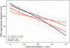 |
Fig. 10. Spatially resolved jittering across the solar disk. RMS values for radial velocities of idealized Fe I lines at λ620 nm are shown for lines of different strengths at excitation potentials χ = 1 and 5 eV. The bold curves show averages over the small simulation area: solid for strong lines; dashed for weak. The curves for χ = 1 eV are black and for 5 eV are red. Multiple thin lines illustrate the differences among different azimuth angles at each center-limb position. |
The jittering is clearly greatest at disk center, gradually decreasing toward the limb. Over much of the disk (50% of the disk area is at μ > 0.71) the stronger line displays the greatest jittering amplitude, but closer to limb the weak line starts to dominate. Near disk center the low-excitation lines jitter more, but that reverses near the limb.
Figure 11 instead shows jittering amplitudes for the full simulated solar disk, for different selected lines, now including the quite strong Mg Iλ457 nm. The even stronger Na I D lines were also measured. These lines will likely not be used for radial-velocity observations, but their data serve to confirm trends already seen in weaker lines. Figure 11 uses data from the full spectrum in the N59 model, and the velocity standard deviations refer to excursions around the mean velocity, as averaged over the simulation sequence.
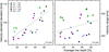 |
Fig. 11. Radial-velocity fluctuations among different line groups, as a function of absorption-line depth. Standard deviations and jittering ranges in the simulation of integrated sunlight are shown, with numbers from the small simulation area (for the actual Sun, divide by a factor of ∼150−200). Stronger and deeper lines display greater amplitudes. The trends extend to the even stronger Na I D1 line which, at 136 and 404 m s−1, is off scale and not included for the fitting of the lines. |
Figures 10 and 11 provide specific model predictions which should be possible to test observationally. For measurements of integrated sunlight, the amplitudes from the simulation area have to be reduced by a large factor, but only by a small amount (if any) in spatially resolved data. These observations should become practical with forthcoming solar telescopes, where light from sections of a spatially somewhat resolved solar image is fed into a high-precision instrument, for example the PoET project at the ESPRESSO spectrometer of ESO in Chile (Leite et al. 2022).
6. Specific spectral regions
There might be spectral features that are both sensitive to fluctuations in the photospheric structure and also practical to observe as possible proxies for excursions in radial velocity. The parameters of strong chromospheric lines have often been used to quantify solar activity, in particular the Ca II H & K emission, Balmer lines from hydrogen, and high-excitation lines from helium.
Nevertheless, these lines all have shortcomings in that they do not precisely reflect local conditions in the photosphere. The strong chromospheric lines are formed mainly in high atmospheric layers with their greater amplitudes in gas motions, driven by magnetic structures, while the weaker He lines are partially excited by X-rays radiating downward from the transition region. On the other hand, precision radial velocities are measured from photospheric spectra alone, and one needs to find features that are particularly sensitive to photospheric changes and that also appear promising to examine in observed spectra.
6.1. The G-band
One interesting region is the G-band. This molecular bandhead around 430 nm mainly consists of transitions between rotational and vibrational sublevels of the CH molecule, blended with numerous atomic lines. The high line density causes an absence of any real continuum across the whole bandhead. As discussed below, the detailed physics of its spectrum formation is not fully understood, although its formation must largely reflect photospheric structures. Line identifications in that region are shown in the Sacramento Peak solar atlas (Beckers et al. 1976), in the IRSOL Second Solar Spectrum atlas (Gandorfer 2002), and in the graphic version (Mrotzek et al. 2016) of the Göttingen solar flux atlas (Reiners et al. 2016). Here we examine the theoretically expected types of variability in advance of actual measurements in Paper II.
6.2. Nonmagnetic G-band spectra
Inside the G-band we do not attempt to follow radial velocities since the massive blending makes it difficult to reliably segregate wavelength displacements from changes in line profiles induced by varying blends driven by temperature fluctuations, for example. Instead, the total spectral flux within different regions is examined. While the exact boundaries of the G-band are not uniquely defined, we adopted the full G-band as 429.84−431.33 nm, with its central core 430.71−430.88 nm (Fig. 12). In its immediately surrounding region, ten reasonably clean Fe I lines were selected to also provide radial-velocity measures: five lines shortward and five longward of the G-band. As a near-continuum reference, 32 segments were selected throughout the region (the same ones later used for observational studies in Paper II). This enabled us to search for differing behavior among spectral features in this region.
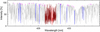 |
Fig. 12. Spectral region surrounding the G-band, indicating measured sections: G-band core (red), full G-band (red + brown), nearby Fe I lines (blue), and pseudocontinuum reference points (red). This plot from the CO 5BOLD N59 model is for the disk center, μ = 1. |
The synthetic G-band spectra at different center-to-limb locations are shown in Fig. 13, together with their ratios. There is a striking dependence such that the relative brightness of the G-band core greatly increases when moving from disk center toward the limb. By contrast, the changes induced by temperature fluctuations in the model are quite modest. Spectral variability is thus more pronounced with respect to the spatial disk position, not with temporal changes. Figure 14 shows the types of correlations present, here selected for μ = 0.79 as representative for much of the emerging flux from the full disk. The data show integrated fluxes of each spectral feature inside its respective wavelength interval (the flux, not the absorption). Naturally, the fluxes increase during hotter instants of the simulation, but the responses differ among different spectral features, with the G-band center showing greater spread than the Fe I lines. However, the radial velocities (being the averages from the ten surrounding Fe I lines) fail to show any obvious correlation with the G-band fluxes.
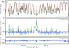 |
Fig. 13. G-band region in synthetic nonmagnetic CO 5BOLD N59 solar spectra. Top frame: intensity spectra at disk center μ = 1 (black), at μ = 0.41 (green), and close to limb μ = 0.09 (red), separately normalized to a very local continuum. Middle frame: spectral ratios relative to disk center for μ = 0.79 (blue) and μ = 0.41 (green). Bottom frame: range of temporal variability illustrated by spectral ratios between snapshot instances of the highest (5806 K) and lowest (5735 K) model temperatures; the same vertical scale as the middle frame is used. |
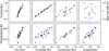 |
Fig. 14. Temporal flickering of the flux in the G-band region of synthetic nonmagnetic CO 5BOLD N59 solar spectra, measured at μ = 0.79. The lower row shows how the effective temperature of the model area at each selected time of the simulation affects features in the region. The G-band flux is plotted in the three leftmost upper frames; the rightmost frame shows radial velocities for the full disk measured in the nearby Fe I lines surrounding the G-band. |
6.3. Magnetic G-band spectra
The complex molecular structure of the G-band implies that its formation may be influenced by numerous effects, as already suggested in the examples of Fig. 13. A primary observation is that magnetic field concentrations in the quiet Sun outside sunspots are spatially largely coincident with areas that are bright in the G-band. Such regions of magnetically affected granulation may cover a non-negligible fraction of the Sun, and may have a different structure and generally exhibit smaller convective wavelength shifts than nonmagnetic areas. Due to their area coverage, these facular and plage regions are the second most significant contributors to the emerging solar radiation (after the extensive regions of nonmagnetic granulation). Much of the solar-cycle variation in apparent solar radial velocity appears to be due to the varying area coverage of these magnetic plage regions (Meunier et al. 2010a,b) and it would be desirable to identify some independent measure of their coverage.
6.3.1. Solar filigree and their magnetic fields
A significant fraction of small-scale magnetic fields in the photosphere are traced by the elongated, sinuous, and crinkly solar filigree, also referred to as bright points (although they are seldom point-like). These small brightness enhancements on subarcsecond scales are now understood to form inside intergranular lanes, near the outer edges of granules, where a local minimum of gas pressure (contributing to the horizontal pressure gradient that drives horizontal gas motions inside and outside granules) is compensated for by the internal magnetic pressure in the flux tubes to achieve a balance with their surroundings.
Solar filigrees were first observed (and named) by Dunn & Zirker (1973). They could be resolved once subarcsecond angular resolution was achieved for imaging the photosphere in narrowband monochromatic images, initially in the far wings of Hα (Dravins 1974; Dunn & Zirker 1973), and later also at other wavelengths, and were soon understood to be largely cospatial with magnetic field concentrations (Mehltretter 1974). The appearance of solar filigrees in various spectral regions on the quiet Sun is described by Berger & Title (2001), Berger et al. (1995, 2004), Langhans et al. (2002), Rouppe van der Voort et al. (2005), and Sánchez Almeida et al. (2004); a review can be found in Bellot Rubio & Orozco Suárez (2019). Among these, observations in the G-band are particularly extensive.
6.3.2. Modeling G-band spectral brightness
Specifics about the G-band formation had already attracted attention a long time ago when observations of its center-to-limb variation suggested that it was formed on a rough and corrugated solar surface (Pecker 1949). More recent work has also mapped the center-to-limb change in convective wavelength shift (Langhans & Schmidt 2002). Solar filigrees are clearly visible in the G-band, and numerous attempts have been made to model their brightness. There is general agreement that the magnetic pressure inside the flux tubes implies a reduced density relative to their surroundings. At a given geometric height, a lower gas pressure causes a lower opacity than in adjacent nonmagnetic regions, enabling us to see deeper and hotter layers. In these deep photospheric layers the CH abundance is reduced by dissociation, and its weaker absorption lines permit more continuum flux to shine through (Carlsson et al. 2004; Kiselman et al. 2001; Shelyag et al. 2004; Schüssler et al. 2003; Stein 2012; Steiner et al. 2001, 2003).
The detailed physics may be more complicated because of effects from non-LTE and 3D radiative line transfer. The hot walls of the flux tube perimeter emit enhanced ultraviolet radiation into the flux tube from its sides, driving the photo-dissociation of the molecules (Steiner et al. 2001). Since the G-band largely contains saturated absorption lines, the amount of its weakening is sensitive to specific line-broadening parameters (Sánchez Almeida et al. 2001). The appearance of the solar surface is further affected by its geometric corrugation: granules have their continuum optical depth unity level some 80 km above the photospheric average, with the magnetic flux tubes some 200−300 km below (Carlsson et al. 2004). For those flux tubes that are inclined relative to the line of sight, the view toward deeper layers may be obstructed.
It should also be noted that not all magnetic elements are necessarily bright. In the quiet Sun G-band brightenings almost always correspond to elements with strong magnetic fields, but in developed plages the correlation becomes weaker (Riethmüller & Solanki 2017). In addition, nonmagnetic bright points may appear, at least in simulations, caused by vertically extending vortices (vortex tubes) in the photosphere (Calvo et al. 2016).
6.3.3. Other molecular bands
The low gas densities and high transparency of fluxtubes also produce enhanced contrast in other spectral features, in particular molecular lines. The violet CN band around 388 nm gives a contrast about 1.4 times greater than the G-band (Kiselman et al. 2001; Rutten et al. 2001; Zakharov et al. 2005), although observationally that short-wavelength region is more demanding than the G-band. Responses for further molecular species are discussed by Berdyugina et al. (2003), Ji et al. (2016), Steiner et al. (2001), and Tritschler & Uitenbroek (2006), that of extended spectra by Norris et al. (2017, 2023).
6.3.4. Magnetic CO 5BOLD models
After injecting a certain magnetic flux in 3D atmospheric structures, its development can be followed into magnetic flux concentrations around intergranular lanes, the magnetic forces being balanced by gas pressure and dynamic effects. The granular motions and their development is disturbed, resulting in a more disrupted granulation structure with a generally smaller convective blueshift. A similar surface magnetoconvection has been modeled, for example, by Beeck et al. (2015a,b), Khomenko et al. (2018), Norris et al. (2023), and Salhab et al. (2018). Spectral synthesis illustrates how the magnetic properties are reflected in the shapes of spectral lines, depending on their magnetic sensitivity (Holzreuter & Solanki 2012, 2015).
Here we use a series of magnetic CO 5BOLD solar models (Ludwig & Steffen 2022; Ludwig et al. 2023). The total net magnetic flux through each horizontal plane is kept constant with the field passing orthogonally through the lower and upper model boundaries, with flux densities of 800, 1600, and 2400 G (80, 160, and 240 mT). This results in a somewhat deformed granulation structure, from which spectra of the G-band region were computed. Values on the order of 160 mT seem characteristic for actual intergranular field strengths in solar filigree (Bellot Rubio & Orozco Suárez 2019; de Wijn et al. 2009; Salhab et al. 2018; Stein 2012). Figure 15 compares the resulting spectra between the zero-field case and that of this representative intergranular flux density of 160 mT. The overall spectral contrast varies with center-to-limb distance and changes sign when approaching the limb.
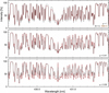 |
Fig. 15. Region around the central G-band in CO 5BOLD simulations for zero magnetic field (dashed black curves) and for B = 1600 G (160 mT) (solid colored curves) for three different center-to-limb positions. The spectra are individually normalized to their local pseudo-continua. |
This is further illustrated in Fig. 16, which shows how the modeled brightness varies across the solar disk for different magnetic field strengths. The G-band flux is given here by the pseudo-continuum levels near the edges of the G-band region: 428.8−428.9 and 431.9−432.0 nm. For moderate flux densities of 800 and 1600 G (80 and 160 mT), this continuum brightness overtakes the zero-field case in positions toward the limb, thus illustrating the crossover to bright facular regions, as distinctly observed in the G-band. For the strongest fields treated here, the continuum intensity becomes faint throughout and apparently something similar to umbral dots begins to form. With even stronger magnetic flux concentrations, surface convection is inhibited and starspots develop, forming umbrae and penumbrae structures, as modeled for different stellar types by Panja et al. (2020). While beyond the scope of the present paper, the corresponding synthetic spectra from such magnetic umbrae and penumbrae may also be combined into a study of fluctuations of spatially resolved features. Pairs of spectral lines with disparate Landé geff-factors, and thus different magnetic sensitivities, should be able to diagnose field properties (Smitha & Solanki 2017), although it might be challenging to perform a detailed synthesis of a full spectrum that precisely incorporates all Zeeman components from all relevant lines. Although the G-band is a very crowded region, instances of somewhat isolated groups of CH lines still exist that are predicted to produce a measurable circular polarization signal through the Zeeman effect (Uitenbroek et al. 2004).
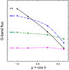 |
Fig. 16. Emission levels in pseudo-continua around the G-band for different magnetic field strengths, relative to the zero-field case at solar disk center, and for different center-to-limb positions. For 800 and 1600 G (80 and 160 mT), the crossover to bright regions (faculae) is seen when moving toward the limb. For the strongest magnetic fields the fluxes become faint, and dark pores begin to form. |
7. Flickering in photometric colors
We now examine what information might be extracted from fluctuations over even broader wavelength regions. Precision measurements of stellar irradiance, made from space, reveal the brightness flickering due to time-variable granulation. This has been theoretically modeled for different spectral types (Lundkvist et al. 2021; Rodríguez Díaz et al. 2022; Samadi et al. 2013a,b), and its observation permits various stellar parameters to be inferred (Bastien et al. 2016; Ness et al. 2018; Van Kooten et al. 2021). This photometric flicker is a concern for exoplanet transit photometry (Sulis et al. 2020).
The connection between simultaneous fluctuations in radial velocity and brightness has been studied. Clear correlations are seen for hotter and more active stars, but are not identified for the smaller amplitudes in cooler stars of solar temperature (Giguere et al. 2016; Oshagh et al. 2017; Sulis et al. 2023). In general, stars with greater photometric variability (probably caused by spots) also have increased levels of jitter in radial velocity. Thus, photometric stability may be used as a criterion to select stars that remain particularly quiet in radial velocity (Hojjatpanah et al. 2020; Tayar et al. 2019).
As discussed above, 3D simulations suggest relations where a 1 m s−1 fluctuation in velocity caused by granular evolution would correspond to a brightness fluctuation on the order of 100 ppm in the light from the full solar disk. However, the longer-term photometric variability of the Sun is dominated by sunspots and active regions, even if searches for photometry as a proxy for short-term variations have been made (Kosiarek & Crossfield 2020).
The required micromagnitude accuracies in absolute stellar fluxes cannot realistically be achieved from the ground, but differential measures of photometric colors might perhaps be feasible from exceptional observing locations (e.g., Schmider et al. 2022), even though they require a good understanding of atmospheric extinction, especially at the shorter wavelengths. A color change reflects a stellar temperature variation and should carry information analogous to the flickering in brightness, and is possibly a candidate for a proxy of excursions in radial velocity. Since our simulations provide absolute fluxes, synthetic broadband photometric colors can be computed. For CO 5BOLD models, certain synthetic colors have been computed by Bonifacio et al. (2018) and Kučinskas et al. (2018), and for the STAGGER grid by Chiavassa et al. (2018).
A photometric system developed to give maximum sensitivity to physical parameters specifically in solar-type stars is the Strömgren system with its four passbands of u − v − b − y, originally proposed by Strömgren (1956, 1966), with later calibrations by Crawford & Barnes (1970) and Önehag et al. (2009), among others. In particular, it is used to study the properties of solar near-twins (e.g., Meléndez et al. 2010; Dalle Mese et al. 2020).
These filters are defined such that the y and b passbands (centered at around 547 and 467 nm) contain no strong spectral features for solar-type type stars, and thus the slope of the spectrum, measured as the color index (b − y), is free of significant effects from line blanketing, becoming an indicator of stellar temperature. The v filter, centered at 411 nm, is placed longward from the region where the Balmer lines from hydrogen begin to crowd as they start to approach the Balmer limit (although the filter transmits Hδ). The near-ultraviolet u filter is centered at 350 nm with its longward part remaining below the Balmer jump, while its shortward part extends to the telluric atmospheric absorption cutoff (Fig. 17). Following standard usage, the fluxes F inside each photometric u − v − b − y band are converted to magnitudes according to m = −2.5 log10(F/F0), where F0 is a reference flux. However, here we are concerned only with the temporal fluctuations in color indices, not their absolute calibration (for an overview of photometric systems, see Bessell 2005).
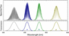 |
Fig. 17. Spectral flux transmitted through four Strömgren u − v − b − y filters (top), and their transmission functions (bottom). |
The exact realization of observational uvby photometry involves nuances such as the construction of the transmission filter optics, properties of the detector (e.g., whether integrating the energy flux inside the filter passband or the number of photons; here the former is applied). We approximate the four filter passbands with Gaussians centered on 350, 411, 467, and 547 nm, with respective standard deviations 12.74, 8.07, 7.64, and 9.77 nm. At the lowest transmission, they are truncated at 0.001 where adjacent filters would start to overlap at filter edges. These profiles closely approximate those used in other works, and are shown in Fig. 17 together with the transmitted flux from the N59 solar model.
From the measurements in these filter passbands, three indices are widely used for stellar classification: the color index (b − y), and the two color-index differences m1 ≡ (v − b)−(b − y), measuring the amount of absorption-line blanketing in the 410 nm region, and c1 ≡ (u − v)−(v − b), quantifying the pressure-dependent Balmer discontinuity. The color index (b − y) reflects stellar temperature and the metal-line index m1 indicates the amount of metallic-line absorption. The Balmer discontinuity index c1 provides a measure of the atmospheric pressure, which, being a function of the surface gravity, gives the stellar luminosity. Greater values of (b − y) imply cooler temperatures; increased metallicity is reflected in a larger m1, and greater luminosity (lower pressure) as a greater value of c1. During the solar activity cycle, spectral brightness changes are driven by magnetic activity, influencing the signals especially in the Strömgren v and b filters (Witzke et al. 2018).
Figures 18 and 19 show the relations between the model fluctuations in the various uvby indices, also relating to the simultaneous jittering in apparent radial velocities for the representative Fe I lines of different strengths. Their parameters of continuum level, depth, width, shape, and wavelength position are those obtained from the five-parameter Gaussian-type fit described above. Clear trends are seen: instances of enhanced continuum brightening correlate with a bluer (b − y) color, weaker line absorption, and an apparently lower metallicity. However, relations among other measures of line depth, line width, and line shape are less obvious or absent, consistent with observational findings by Oshagh et al. (2017) and Sulis et al. (2023).
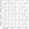 |
Fig. 18. Relations between parameters of a representative Fe I line of medium strength at 520 nm (Fig. 2) in integrated sunlight from the N59 model, and flickering in photometric Strömgren indices. Quantitites refer to relative variations over the small simulation area. |
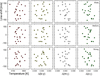 |
Fig. 19. Search for relations between radial velocities of Fe I lines of different strengths at 520 nm (Fig. 2) and photometric Strömgren indices in integrated sunlight, as computed over the small simulation area of the N59 model (for the actual Sun, divide the numerical values by a factor of ∼150−200). The rows show (from top down) the weak, medium, and strong lines. |
Irrespective of whether correlations with specific spectral signatures can be identified, the data illustrate what amplitudes might be expected in the flickering of full-disk sunlight in different color indices. For the data shown in Fig. 18, the RMS fluctuations in (b − y), m1, and c1 are respectively 0.0023, 0.0033, and 0.0017. The greatest changes occur in m1, due to changing absorption-line strengths in the blue, while the modulation of the luminosity index is only half that. In actual full-disk sunlight, these amplitudes should be divided by a factor of ∼150 or 200; they then shrink from a few millimagnitudes to only 10 or 20 μmag. The corresponding RMS fluctuations in the continuum level of 1.4% at 525 nm over the model area correspond to ∼100 ppm in full integrated sunlight, in line with what was deduced by Cegla et al. (2019). Plots for separate center-to-limb positions show the relative fluctuation amplitudes increasing from disk center toward the limb, but are not qualitatively different. The expected performance of space missions such as PLATO readily permits the detection of such levels of photometric variability (Heller et al. 2022; Morris et al. 2020), although their search for exoplanets will also depend on how to segregate other types of stellar variability. Observed day-to-day solar irradiance fluctuations, driven by the presence of faculae and appearance of spots, are typically greater by an order of magnitude, and those during a solar activity cycle by another order of magnitude (Lean et al. 2020; Marchenko et al. 2019).
8. Lack of correlation in other line parameters
Relations were sought between the velocity jittering and other spectral-line parameters that might be suspected to vary in phase during the simulation sequences. However, as seen in Fig. 20, there appears to be no sensible correlation with continuum brightness, line width, or line shape (the quantities in the five-parameter Gaussian-type fit described in Sect. 4.1). An exception is that a weak relation appears to exist with line depth, at least for the strongest lines. Such a correlation is actually expected, and was seen in clean disk-center data by Dravins et al. (2021b). Locations of increased irradiance display enhanced convective blueshift combined with a stronger line absorption, caused by enhanced vertical gradients in regions of line formation. However, while this is seen when granules are viewed directly from above, the effect rapidly diminishes away from disk center, and largely gets washed out in the integrated sunlight of Fig. 20.
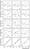 |
Fig. 20. Radial velocities showing lack of correlation with several plausibly anticipated fluctuations in various line parameters. No correlations were found here, except a hint of a line depth dependence in the strongest lines. The measures for line depth, width, and shape are normalized to 100% for the averages over the simulation sequence. The calculations are for integrated sunlight from the small simulation area of the N59 model (for the actual Sun, divide the lineshift values by a factor of ∼150−200). |
9. Search for Earth-like exoplanets
Under realistic conditions, the spectral-line parameter that can be most precisely measured is its wavelength, rather than the depth, width, or shape, which are more sensitive to the exact adjustments in the spectroscopic instrumentation. Given the results in this paper, this is satisfactory since significant mutual correlations between line groups could be identified for precisely this wavelength jittering. Various other parameters, such as the fluctuating widths or depths of absorption lines, or flickering in broadband photometric indices fail to show convincing correlations with excursions in radial velocity.
Using the results from hydrodynamic simulations, it is thus possible to identify patterns of velocity jittering. Characteristics of simultaneous jittering in radial velocity between different groups of lines, as shown in Figs. 8 and 9, distinguish the radial-velocity contributions originating from fluctuations in photospheric granulation, the signature of which should be possible to deduce and deduct.
In practice, this will require obtaining radial-velocity measures for groups of individually selected spectral lines within distinct batches of stronger and weaker lines, and in different wavelength regions. Jittering amplitudes from each homogeneous line group are expected to show systematic differences, such that the excursions of strong short-wavelength Fe II lines would be greater by a certain factor than, for example, those of weak Fe I lines at long wavelengths. A “matched filter” fitted to such a variability pattern should identify the component of velocity jittering that is specific to granular convection. While the present work permits us to estimate the rough parameters for such a filter, its more precise numbers will require more extensive simulations, the validity of which could be confirmed in such spatially resolved observations that are feasible already with current instrumentation, as suggested in Figs. 10 and 11. Other sources of jittering originate from oscillations and various magnetic phenomena over other timescales, requiring separate attention.
The observational requirements are stringent, but probably not impossible. The total jittering amplitude in full-disk sunlight amounts to ∼1−2 m s−1, with differences between the various line groups perhaps one-tenth of that. To mitigate these fluctuations thus requires recognizing the characteristic patterns of dissimilar lineshifts among classes of various spectral lines with precisions ∼10 cm s−1 for each absorption-line group. Although certainly challenging, these requirements correspond to what is required in any case in searches for truly Earth-like exoplanets, for example HARPS-3 (Farret Jentink et al. 2022; Thompson et al. 2016) or ANDES (Marconi et al. 2022).
From other considerations, it has also been recognized that there is additional information contained in individual spectral lines, as compared to statistical correlation functions (Al Moulla et al. 2022; Cretignier et al. 2020; Dumusque 2018; Meunier et al. 2017b; Wise et al. 2022). Recent efforts for the Sun seen as a star include the extraction of radial-velocity data separately from lines with different depths (Miklos et al. 2020), and the study of how spectral portions differ during epochs of magnetically more active or quieter periods (Thompson et al. 2020).
Most of our present modeling is limited to the nonmagnetic photosphere and to such short-term fluctuations that are comparable to granular evolution timescales. This quiet photosphere covers the largest fraction of the solar surface and contributes the greatest part of the total flux (and presumably that of other solar-type stars) but magnetic features seem responsible for much of the variability over the longer timescales of stellar rotation and activity cycles.
The following Paper II (Dravins & Ludwig, in prep.) will explore the observed solar microvariability on these longer timescales. The aim is to identify further measurable photospheric parameters that might be used as proxies for radial-velocity fluctuations.
The Vienna Atomic Line Database of atomic and molecular transition parameters of astronomical interest.
The term hyper-high is used to denote spectral resolutions λ/Δλ ≳ 106 since ultra-high is already in common use to describe spectrometers with the much lower resolutions of “only” ∼200 000.
Acknowledgments
The work by D.D. is supported by grants from The Royal Physiographic Society of Lund. H.G.L. gratefully acknowledges financial support by the Deutsche Forschungsgemeinschaft (DFG, German Research Foundation) – Project ID 138713538–SFB 881 (‘The Milky Way System’, subproject A04). Extensive use was made of NASA’s ADS Bibliographic Services and the arXiv® distribution service. We thank the referee for very detailed and insightful comments.
References
- Al Moulla, K., Dumusque, X., Cretignier, M., et al. 2022, A&A, 664, A34 [NASA ADS] [CrossRef] [EDP Sciences] [Google Scholar]
- Asplund, M. 2005, ARA&A, 43, 481 [Google Scholar]
- Bastien, F. A., Stassun, K. G., Basri, G., et al. 2016, ApJ, 818, 43 [NASA ADS] [CrossRef] [Google Scholar]
- Beckers, J. M., Bridges, C. A., & Gilliam, L. B. 1976, Environmental Research Papers (Hanscom Ma: Air Force Geophysics Laboratory) [Google Scholar]
- Beeck, B., Schüssler, M., Cameron, R. H., et al. 2015a, A&A, 581, A42 [NASA ADS] [CrossRef] [EDP Sciences] [Google Scholar]
- Beeck, B., Schüssler, M., Cameron, R. H., et al. 2015b, A&A, 581, A43 [NASA ADS] [CrossRef] [EDP Sciences] [Google Scholar]
- Bellot Rubio, L., & Orozco Suárez, D. 2019, Liv. Rev. Sol. Phys., 16, 1 [Google Scholar]
- Berdyugina, S. V., Solanki, S. K., & Frutiger, C. 2003, A&A, 412, 513 [NASA ADS] [CrossRef] [EDP Sciences] [Google Scholar]
- Bergemann, M., Gallagher, A. J., Eitner, P., et al. 2019, A&A, 631, A80 [NASA ADS] [CrossRef] [EDP Sciences] [Google Scholar]
- Berger, T. E., & Title, A. M. 2001, ApJ, 553, 449 [NASA ADS] [CrossRef] [Google Scholar]
- Berger, T. E., Schrijver, C. J., Shine, R. A., et al. 1995, ApJ, 454, 531 [NASA ADS] [CrossRef] [Google Scholar]
- Berger, T. E., Rouppe van der Voort, L. H. M., Löfdahl, M. G., et al. 2004, A&A, 428, 613 [NASA ADS] [CrossRef] [EDP Sciences] [Google Scholar]
- Berke, D. A., Murphy, M. T., Flynn, C., et al. 2023a, MNRAS, 519, 1221 [Google Scholar]
- Berke, D. A., Murphy, M. T., Flynn, C., et al. 2023b, MNRAS, 519, 1238 [Google Scholar]
- Bessell, M. S. 2005, ARA&A, 43, 293 [NASA ADS] [CrossRef] [Google Scholar]
- Biazzo, K., Frasca, A., Catalano, S., et al. 2007, Astron. Nachr., 328, 938 [NASA ADS] [CrossRef] [Google Scholar]
- Blackman, R. T., Fischer, D. A., Jurgenson, C. A., et al. 2020, AJ, 159, 238 [CrossRef] [Google Scholar]
- Bonifacio, P., Caffau, E., Ludwig, H.-G., et al. 2018, A&A, 611, A68 [NASA ADS] [CrossRef] [EDP Sciences] [Google Scholar]
- Bouchy, F., Doyon, R., Artigau, É., et al. 2017, The Messenger, 169, 21 [NASA ADS] [Google Scholar]
- Calvo, F., Steiner, O., & Freytag, B. 2016, A&A, 596, A43 [NASA ADS] [CrossRef] [EDP Sciences] [Google Scholar]
- Carlsson, M., Stein, R. F., Nordlund, Å., et al. 2004, ApJ, 610, L137 [NASA ADS] [CrossRef] [Google Scholar]
- Cegla, H. M., Watson, C. A., Shelyag, S., et al. 2019, ApJ, 879, 55 [NASA ADS] [CrossRef] [Google Scholar]
- Chiavassa, A., Casagrande, L., Collet, R., et al. 2018, A&A, 611, A11 [NASA ADS] [CrossRef] [EDP Sciences] [Google Scholar]
- Coffinet, A., Lovis, C., Dumusque, X., et al. 2019, A&A, 629, A27 [NASA ADS] [CrossRef] [EDP Sciences] [Google Scholar]
- Collier Cameron, A., Mortier, A., Phillips, D., et al. 2019, MNRAS, 487, 1082 [Google Scholar]
- Collier Cameron, A., Ford, E. B., Shahaf, S., et al. 2021, MNRAS, 505, 1699 [NASA ADS] [CrossRef] [Google Scholar]
- Cosentino, R., Lovis, C., Pepe, F., et al. 2012, Proc. SPIE, 8446, 84461V [Google Scholar]
- Cranmer, S. R., Bastien, F. A., Stassun, K. G., et al. 2014, ApJ, 781, 124 [CrossRef] [Google Scholar]
- Crass, J., Gaudi, B. S., Leifer, S., et al. 2021, ArXiv e-prints [arXiv:2107.14291] [Google Scholar]
- Crass, J., Aikens, D., Mason, J., et al. 2022, Proc. SPIE, 12184, 121841P [NASA ADS] [Google Scholar]
- Crawford, D. L., & Barnes, J. V. 1970, AJ, 75, 978 [NASA ADS] [CrossRef] [Google Scholar]
- Cretignier, M., Dumusque, X., Allart, R., et al. 2020, A&A, 633, A76 [NASA ADS] [CrossRef] [EDP Sciences] [Google Scholar]
- Dalle Mese, G., López-Cruz, O., Schuster, W. J., et al. 2020, MNRAS, 494, 2995 [NASA ADS] [CrossRef] [Google Scholar]
- de Beurs, Z. L., Vanderburg, A., Shallue, C. J., et al. 2022, AJ, 164, 49 [NASA ADS] [CrossRef] [Google Scholar]
- de Wijn, A. G., Stenflo, J. O., Solanki, S. K., et al. 2009, Space. Sci. Rev., 144, 275 [NASA ADS] [CrossRef] [Google Scholar]
- Donati, J.-F., Kouach, D., Moutou, C., et al. 2020, MNRAS, 498, 5684 [NASA ADS] [CrossRef] [Google Scholar]
- Dravins, D. 1974, IAU Symp., 56, 257 [NASA ADS] [Google Scholar]
- Dravins, D. 1989, Proc. NATO ASI Ser. C, 263, 153 [NASA ADS] [Google Scholar]
- Dravins, D., & Nordlund, Å. 1990, A&A, 228, 184 [NASA ADS] [Google Scholar]
- Dravins, D., Ludwig, H.-G., Dahlén, E., et al. 2017a, A&A, 605, A90 [NASA ADS] [CrossRef] [EDP Sciences] [Google Scholar]
- Dravins, D., Ludwig, H.-G., Dahlén, E., et al. 2017b, A&A, 605, A91 [NASA ADS] [CrossRef] [EDP Sciences] [Google Scholar]
- Dravins, D., Gustavsson, M., & Ludwig, H.-G. 2018, A&A, 616, A144 [NASA ADS] [CrossRef] [EDP Sciences] [Google Scholar]
- Dravins, D., Ludwig, H.-G., & Freytag, B. 2021a, A&A, 649, A16 [NASA ADS] [CrossRef] [EDP Sciences] [Google Scholar]
- Dravins, D., Ludwig, H.-G., & Freytag, B. 2021b, A&A, 649, A17 [NASA ADS] [CrossRef] [EDP Sciences] [Google Scholar]
- Dumusque, X. 2016, A&A, 593, A5 [NASA ADS] [CrossRef] [EDP Sciences] [Google Scholar]
- Dumusque, X. 2018, A&A, 620, A47 [NASA ADS] [CrossRef] [EDP Sciences] [Google Scholar]
- Dumusque, X., Udry, S., Lovis, C., et al. 2011, A&A, 525, A140 [NASA ADS] [CrossRef] [EDP Sciences] [Google Scholar]
- Dumusque, X., Glenday, A., Phillips, D. F., et al. 2015, ApJ, 814, L21 [Google Scholar]
- Dumusque, X., Borsa, F., Damasso, M., et al. 2017, A&A, 598, A133 [NASA ADS] [CrossRef] [EDP Sciences] [Google Scholar]
- Dumusque, X., Cretignier, M., Sosnowska, D., et al. 2021, A&A, 648, A103 [NASA ADS] [CrossRef] [EDP Sciences] [Google Scholar]
- Dunn, R. B., & Zirker, J. B. 1973, Sol. Phys., 33, 281 [NASA ADS] [Google Scholar]
- Farret Jentink, C., Mortier, A., Snik, F., et al. 2022, Proc. SPIE, 12182, 1218231 [NASA ADS] [Google Scholar]
- Fischer, D. A., Anglada-Escude, G., Arriagada, P., et al. 2016, PASP, 128, 066001 [Google Scholar]
- Freytag, B., Steffen, M., Ludwig, H.-G., et al. 2012, J. Comp. Phys., 231, 919 [NASA ADS] [CrossRef] [Google Scholar]
- Gandorfer, A. 2002, The Second Solar Spectrum: A High Spectral Resolution Polarimetric Survey of Scattering Polarization at the Solar Limb in Graphical Representation (Zurich: vdf Hochschulverlag) [Google Scholar]
- Giguere, M. J., Fischer, D. A., Zhang, C. X. Y., et al. 2016, ApJ, 824, 150 [Google Scholar]
- Gibson, S. R., Howard, A. W., Marcy, G. W., et al. 2016, Proc. SPIE, 9908, 990870 [NASA ADS] [CrossRef] [Google Scholar]
- Gilbert, J., Bergmann, C., Bloxham, G., et al. 2018, Proc. SPIE, 10702, 107020Y [NASA ADS] [Google Scholar]
- Gray, D. F. 1994, PASP, 106, 1248 [NASA ADS] [CrossRef] [Google Scholar]
- Hall, R. D., Thompson, S. J., Handley, W., et al. 2018, MNRAS, 479, 2968 [NASA ADS] [CrossRef] [Google Scholar]
- Halverson, S., Terrien, R., Mahadevan, S., et al. 2016, Proc. SPIE, 9908, 99086P [NASA ADS] [CrossRef] [Google Scholar]
- Hara, N. C., & Ford, E. B. 2023, Ann. Rev. Stat. Appl., 10, 623 [NASA ADS] [CrossRef] [Google Scholar]
- Haywood, R. D., Collier Cameron, A., Unruh, Y. C., et al. 2016, MNRAS, 457, 3637 [Google Scholar]
- Heiter, U., Lind, K., Asplund, M., et al. 2015, Phys. Scr., 90, 054010 [Google Scholar]
- Heller, R., Harre, J.-V., & Samadi, R. 2022, A&A, 665, A11 [NASA ADS] [CrossRef] [EDP Sciences] [Google Scholar]
- Hobson, M. J., Bouchy, F., Cook, N. J., et al. 2021, A&A, 648, A48 [NASA ADS] [CrossRef] [EDP Sciences] [Google Scholar]
- Hojjatpanah, S., Oshagh, M., Figueira, P., et al. 2020, A&A, 639, A35 [NASA ADS] [CrossRef] [EDP Sciences] [Google Scholar]
- Holzreuter, R., & Solanki, S. K. 2012, A&A, 547, A4 [Google Scholar]
- Holzreuter, R., & Solanki, S. K. 2015, A&A, 582, A101 [NASA ADS] [CrossRef] [EDP Sciences] [Google Scholar]
- Ji, K.-F., Xiong, J.-P., Xiang, Y.-Y., et al. 2016, Res. Astron. Astrophys., 16, 78 [Google Scholar]
- Jurgenson, C., Fischer, D., McCracken, T., et al. 2016, Proc. SPIE, 9908, 99086T [NASA ADS] [CrossRef] [Google Scholar]
- Kallinger, T., De Ridder, J., Hekker, S., et al. 2014, A&A, 570, A41 [NASA ADS] [CrossRef] [EDP Sciences] [Google Scholar]
- Kanodia, S., Halverson, S., Ninan, J. P., et al. 2021, ApJ, 912, 15 [NASA ADS] [CrossRef] [Google Scholar]
- Khomenko, E., Vitas, N., Collados, M., et al. 2018, A&A, 618, A87 [NASA ADS] [CrossRef] [EDP Sciences] [Google Scholar]
- Kiselman, D., Rutten, R. J., & Plez, B. 2001, IAU Symp., 203, 287 [NASA ADS] [Google Scholar]
- Kitiashvili, I., Granovsky, S., & Wray, A. 2023, IAU Symp., 362, 324 [NASA ADS] [Google Scholar]
- Kosiarek, M. R., & Crossfield, I. J. M. 2020, AJ, 159, 271 [NASA ADS] [CrossRef] [Google Scholar]
- Kučinskas, A., Klevas, J., Ludwig, H.-G., et al. 2018, A&A, 613, A24 [NASA ADS] [CrossRef] [EDP Sciences] [Google Scholar]
- Langhans, K., & Schmidt, W. 2002, A&A, 382, 312 [NASA ADS] [CrossRef] [EDP Sciences] [Google Scholar]
- Langhans, K., Schmidt, W., & Tritschler, A. 2002, A&A, 394, 1069 [NASA ADS] [CrossRef] [EDP Sciences] [Google Scholar]
- Lanza, A. F., Molaro, P., Monaco, L., et al. 2016, A&A, 587, A103 [NASA ADS] [CrossRef] [EDP Sciences] [Google Scholar]
- Lanza, A. F., Collier Cameron, A., & Haywood, R. D. 2019, MNRAS, 486, 3459 [NASA ADS] [CrossRef] [Google Scholar]
- Lean, J. L., Coddington, O., Marchenko, S. V., et al. 2020, Earth Space Sci., 7, 00645 [NASA ADS] [CrossRef] [Google Scholar]
- Leite, I., Cabral, A., Abreu, M., & Santos, N. 2022, J. Phys.: Conf. Ser., 2407, 012020 [NASA ADS] [CrossRef] [Google Scholar]
- Lienhard, F., Mortier, A., Cegla, H. M., et al. 2023, MNRAS, 522, 5862 [NASA ADS] [CrossRef] [Google Scholar]
- Ludwig, H.-G. 2006, A&A, 445, 661 [NASA ADS] [CrossRef] [EDP Sciences] [Google Scholar]
- Ludwig, H.-G., & Steffen, M. 2008, Precision Spectroscopy in Astrophysics, ESO Astrophysics Symposia (Springer), 133 [CrossRef] [Google Scholar]
- Ludwig, H.-G., & Steffen, M. 2022, https://zenodo.org/records/7447826 [Google Scholar]
- Ludwig, H. G., Steffen, M., & Freytag, B. 2023, A&A, in press, https://doi.org/10.1051/0004-6361/202346783 [Google Scholar]
- Lundkvist, M. S., Ludwig, H.-G., Collet, R., et al. 2021, MNRAS, 501, 2512 [CrossRef] [Google Scholar]
- Mahadevan, S., Ramsey, L. W., Terrien, R., et al. 2014, Proc. SPIE, 9147, 91471G [NASA ADS] [CrossRef] [Google Scholar]
- Maldonado, J., Phillips, D. F., Dumusque, X., et al. 2019, A&A, 627, A118 [NASA ADS] [CrossRef] [EDP Sciences] [Google Scholar]
- Marchenko, S. V., Woods, T. N., DeLand, M. T., et al. 2019, Earth Space Sci., 6, 2379 [NASA ADS] [CrossRef] [Google Scholar]
- Marchwinski, R. C., Mahadevan, S., Robertson, P., et al. 2015, ApJ, 798, 63 [Google Scholar]
- Marconi, A., Abreu, M., Adibekyan, V., et al. 2022, Proc. SPIE, 12184, 1218424 [NASA ADS] [Google Scholar]
- Mayor, M., Pepe, F., Queloz, D., et al. 2003, The Messenger, 114, 20 [NASA ADS] [Google Scholar]
- Mehltretter, J. P. 1974, Sol. Phys., 38, 43 [CrossRef] [Google Scholar]
- Meléndez, J., Schuster, W. J., Silva, J. S., et al. 2010, A&A, 522, A98 [NASA ADS] [CrossRef] [EDP Sciences] [Google Scholar]
- Meunier, N., & Lagrange, A.-M. 2019, A&A, 625, L6 [NASA ADS] [CrossRef] [EDP Sciences] [Google Scholar]
- Meunier, N., & Lagrange, A. M. 2020, A&A, 642, A157 [NASA ADS] [CrossRef] [EDP Sciences] [Google Scholar]
- Meunier, N., Desort, M., & Lagrange, A.-M. 2010a, A&A, 512, A39 [NASA ADS] [CrossRef] [EDP Sciences] [Google Scholar]
- Meunier, N., Lagrange, A.-M., & Desort, M. 2010b, A&A, 519, A66 [NASA ADS] [CrossRef] [EDP Sciences] [Google Scholar]
- Meunier, N., Lagrange, A.-M., Borgniet, S., et al. 2015, A&A, 583, A118 [NASA ADS] [CrossRef] [EDP Sciences] [Google Scholar]
- Meunier, N., Lagrange, A.-M., Mbemba Kabuiku, L., et al. 2017a, A&A, 597, A52 [NASA ADS] [CrossRef] [EDP Sciences] [Google Scholar]
- Meunier, N., Lagrange, A.-M., & Borgniet, S. 2017b, A&A, 607, A6 [NASA ADS] [CrossRef] [EDP Sciences] [Google Scholar]
- Miklos, M., Milbourne, T. W., Haywood, R. D., et al. 2020, ApJ, 888, 117 [Google Scholar]
- Morris, B. M., Bobra, M. G., Agol, E., et al. 2020, MNRAS, 493, 5489 [NASA ADS] [CrossRef] [Google Scholar]
- Mrotzek, N., Lemke, U., Hinrichs, J., et al. 2016, Spectral Atlas of the Sun from 405 to 2300 nm, Institut für Astrophysik, Göttingen, http://www.astro.physik.uni-goettingen.de/research/flux_atlas/atlas_print_version_4000-23000.pdf [Google Scholar]
- Murphy, M. T., Berke, D. A., Liu, F., et al. 2022, Science, 378, 634 [NASA ADS] [CrossRef] [Google Scholar]
- Nèmec, N.-E., Işık, E., Shapiro, A. I., et al. 2020, A&A, 638, A56 [NASA ADS] [CrossRef] [EDP Sciences] [Google Scholar]
- Ness, M. K., Silva Aguirre, V., Lund, M. N., et al. 2018, ApJ, 866, 15 [NASA ADS] [CrossRef] [Google Scholar]
- Nordlund, Å., Stein, R. F., & Asplund, M. 2009, Liv. Rev. Sol. Phys., 6, 2 [Google Scholar]
- Norris, C. M., Beeck, B., Unruh, Y. C., et al. 2017, A&A, 605, A45 [NASA ADS] [CrossRef] [EDP Sciences] [Google Scholar]
- Norris, C. M., Unruh, Y. C., Witzke, V., et al. 2023, MNRAS, 524, 1139 [NASA ADS] [CrossRef] [Google Scholar]
- Önehag, A., Gustafsson, B., Eriksson, K., et al. 2009, A&A, 498, 527 [NASA ADS] [CrossRef] [EDP Sciences] [Google Scholar]
- Oshagh, M., Santos, N. C., Figueira, P., et al. 2017, A&A, 606, A107 [NASA ADS] [CrossRef] [EDP Sciences] [Google Scholar]
- Panja, M., Cameron, R., & Solanki, S. K. 2020, ApJ, 893, 113 [CrossRef] [Google Scholar]
- Pecker, J.-C. 1949, Ann. Astrophys., 12, 9 [NASA ADS] [Google Scholar]
- Pepe, F., Molaro, P., Cristiani, S., et al. 2014, Astron. Nachr., 335, 8 [Google Scholar]
- Pepe, F., Cristiani, S., Rebolo, R., et al. 2021, A&A, 645, A96 [NASA ADS] [CrossRef] [EDP Sciences] [Google Scholar]
- Plavchan, P., Vasisht, G., Beichman, C., et al. 2019, EarthFinder Probe Mission Concept Study, NASA-JPL-George Mason University-Caltech, 66 [Google Scholar]
- Quirrenbach, A., Amado, P. J., Caballero, J. A., et al. 2014, Proc. SPIE, 9147, 91471F [Google Scholar]
- Quirrenbach, A., Amado, P. J., Ribas, I., et al. 2018, Proc. SPIE, 10702, 107020W [Google Scholar]
- Rackham, B. V., Espinoza, N., Berdyugina, S. V., et al. 2023, RAS Tech. Instrum., 2, 148 [NASA ADS] [CrossRef] [Google Scholar]
- Reiners, A., Mrotzek, N., Lemke, U., et al. 2016, A&A, 587, A65 [NASA ADS] [CrossRef] [EDP Sciences] [Google Scholar]
- Riethmüller, T. L., & Solanki, S. K. 2017, A&A, 598, A123 [NASA ADS] [CrossRef] [EDP Sciences] [Google Scholar]
- Rodríguez Díaz, L. F., Bigot, L., Aguirre Børsen-Koch, V., et al. 2022, MNRAS, 514, 1741 [CrossRef] [Google Scholar]
- Rouppe van der Voort, L. H. M., Hansteen, V. H., Carlsson, M., et al. 2005, A&A, 435, 327 [NASA ADS] [CrossRef] [EDP Sciences] [Google Scholar]
- Rutten, R. J., Kiselman, D., Rouppe van der Voort, L., et al. 2001, ASP Conf. Ser., 236, 445 [NASA ADS] [Google Scholar]
- Ryabchikova, T., Piskunov, N., Kurucz, R. L., et al. 2015, Phys. Scr., 90, 054005 [Google Scholar]
- Salhab, R. G., Steiner, O., Berdyugina, S. V., et al. 2018, A&A, 614, A78 [NASA ADS] [CrossRef] [EDP Sciences] [Google Scholar]
- Samadi, R., Belkacem, K., & Ludwig, H.-G. 2013a, A&A, 559, A39 [NASA ADS] [CrossRef] [EDP Sciences] [Google Scholar]
- Samadi, R., Belkacem, K., Ludwig, H.-G., et al. 2013b, A&A, 559, A40 [NASA ADS] [CrossRef] [EDP Sciences] [Google Scholar]
- Sánchez Almeida, J., Asensio Ramos, A., Trujillo Bueno, J., et al. 2001, ApJ, 555, 978 [CrossRef] [Google Scholar]
- Sánchez Almeida, J., Márquez, I., Bonet, J. A., et al. 2004, ApJ, 609, L91 [CrossRef] [Google Scholar]
- Schmider, F.-X., Abe, L., Agabi, A., et al. 2022, Proc. SPIE, 12182, 121822O [NASA ADS] [Google Scholar]
- Schüssler, M., Shelyag, S., Berdyugina, S., et al. 2003, ApJ, 597, L173 [CrossRef] [Google Scholar]
- Schwab, C., Rakich, A., Gong, Q., et al. 2016, Proc. SPIE, 9908, 99087H [NASA ADS] [Google Scholar]
- Seifahrt, A., Stürmer, J., Bean, J. L., et al. 2018, Proc. SPIE, 10702, 107026D [NASA ADS] [Google Scholar]
- Seifahrt, A., Bean, J. L., Kasper, D., et al. 2022, Proc. SPIE, 12184, 121841G [NASA ADS] [Google Scholar]
- Shelyag, S., Schüssler, M., Solanki, S. K., et al. 2004, A&A, 427, 335 [NASA ADS] [CrossRef] [EDP Sciences] [Google Scholar]
- Smitha, H. N., & Solanki, S. K. 2017, A&A, 608, A111 [NASA ADS] [CrossRef] [EDP Sciences] [Google Scholar]
- Stein, R. F. 2012, Liv. Rev. Sol. Phys., 9, 4 [Google Scholar]
- Steiner, O., Hauschildt, P. H., & Bruls, J. 2001, A&A, 372, L13 [NASA ADS] [CrossRef] [EDP Sciences] [Google Scholar]
- Steiner, O., Hauschildt, P. H., & Bruls, J. 2003, Astron. Nachr., 324, 398 [NASA ADS] [CrossRef] [Google Scholar]
- Strömgren, B. 1956, Vistas Astron., 2, 1336 [CrossRef] [Google Scholar]
- Strömgren, B. 1966, ARA&A, 4, 433 [CrossRef] [Google Scholar]
- Sulis, S., Lendl, M., Hofmeister, S., et al. 2020, A&A, 636, A70 [NASA ADS] [CrossRef] [EDP Sciences] [Google Scholar]
- Sulis, S., Lendl, M., Cegla, H. M., et al. 2023, A&A, 670, A24 [NASA ADS] [CrossRef] [EDP Sciences] [Google Scholar]
- Szentgyorgyi, A., Baldwin, D., Barnes, S., et al. 2018, Proc. SPIE, 10702, 107021R [NASA ADS] [Google Scholar]
- Tayar, J., Stassun, K. G., & Corsaro, E. 2019, ApJ, 883, 195 [Google Scholar]
- Thompson, S. J., Queloz, D., Baraffe, I., et al. 2016, Proc. SPIE, 9908, 99086F [NASA ADS] [CrossRef] [Google Scholar]
- Thompson, A. P. G., Watson, C. A., Haywood, R. D., et al. 2020, MNRAS, 494, 4279 [Google Scholar]
- Tremblay, P.-E., Ludwig, H.-G., Freytag, B., et al. 2013, A&A, 557, A7 [NASA ADS] [CrossRef] [EDP Sciences] [Google Scholar]
- Tritschler, A., & Uitenbroek, H. 2006, ApJ, 648, 741 [NASA ADS] [CrossRef] [Google Scholar]
- Uitenbroek, H., Miller-Ricci, E., Asensio Ramos, A., et al. 2004, ApJ, 604, 960 [NASA ADS] [CrossRef] [Google Scholar]
- Van Kooten, S. J., Anders, E. H., & Cranmer, S. R. 2021, ApJ, 913, 69 [NASA ADS] [CrossRef] [Google Scholar]
- Wise, A., Plavchan, P., Dumusque, X., et al. 2022, ApJ, 930, 121 [NASA ADS] [CrossRef] [Google Scholar]
- Witzke, V., Shapiro, A. I., Solanki, S. K., et al. 2018, A&A, 619, A146 [NASA ADS] [CrossRef] [EDP Sciences] [Google Scholar]
- Zakharov, V., Gandorfer, A., Solanki, S. K., et al. 2005, A&A, 437, L43 [NASA ADS] [CrossRef] [EDP Sciences] [Google Scholar]
- Zhao, L. L., Fischer, D. A., Ford, E. B., et al. 2022, AJ, 163, 171 [NASA ADS] [CrossRef] [Google Scholar]
All Tables
All Figures
|
Fig. 1. Synthetic solar spectra from the CO 5BOLD N59 model simulation, centered on 525 nm. The spectra are seen over gradually narrower wavelength ranges, decreasing by a factor of 3 for each row from top down. Left column: disk center: μ = cos θ = 1; middle: μ = 0.41; right: μ = 0.09. The intensity scale is common for all frames, and illustrates how the limb darkening is more pronounced at shorter wavelengths. |
| In the text | |
|
Fig. 2. Examples of selected lines. Shown here are Fe I lines around λ525 nm from the N59 model. Top: synthetic spectra at solar disk center, μ = 1; bottom: μ = 0.41. The clean lines selected for detailed analysis are shown in red: strong, medium, and weak labeled A, B, and C, respectively. The lines become noticeably broader toward the limb. |
| In the text | |
|
Fig. 3. Example of temporal variability of line profiles during the N59 simulation sequence, sampled at 20 instances of time. Left columns: strong Fe Iλ436.59 nm, χ = 2.99 eV line (in the shortward blue); right columns: weak Fe Iλ675.27 nm, χ = 4.64 eV line (in the longward red). The upper row shows profiles for the disk center μ = 1; the bottom row shows integrated sunlight, corresponding to a full solar disk, synthesized using center-to-limb profiles from the small simulation area. The magnified images on the right show the line centers on a uniform wavelength scale in units of radial velocity (top); the tick marks on the vertical axes correspond to those for the full profiles. |
| In the text | |
|
Fig. 4. Temporal variability of idealized line profiles during the N58 simulation sequence, sampled at 19 instances of time. Left columns: differently strong Fe I lines at λ620 nm, χ = 3 eV; right columns: lines of similar strength, but with different lower excitation potentials, χ = 1 eV (black) and 5 eV (red). Top row: profiles at disk center μ = 1; bottom row: μ = 0.59. To limit cluttering, profiles are shown for only two (orthogonal) azimuth angles. The right frames show zoomed-in images of the line centers, with wavelength scales equal to those in Fig. 3; the tick marks on the vertical axes correspond to those for the full profiles. |
| In the text | |
|
Fig. 5. Example of a five-parameter Gaussian-type fit to a typical Fe I line profile in integrated sunlight. Profiles from each temporal snapshot are shown as thin black lines; their average is shown as a dashed red line, and the fitted profile as yellow circles. In the zoomed-in image at the right, the tick marks of the vertical scale correspond to those in the left frame. |
| In the text | |
|
Fig. 6. Radial-velocity shifts of synthetic isolated Fe I lines at λ620 nm in the N58 model. Relations between shifts at solar disk center, μ = 1, for weak, medium, and strong lines are shown for different excitation potentials. Each point represents one temporal snapshot during the simulation. The dotted reference lines give the identity relations; the other fitted lines indicate how the dependence of convective blueshift on line strength and excitation potential generally remains valid, even when the spatially averaged radial velocity fluctuates. |
| In the text | |
|
Fig. 7. Differences in radial-velocity shifts between lines with different strengths (but similar excitation potentials). These data at μ = 1 are from synthetic isolated Fe I lines at λ620 nm in the N58 model. Each point represents the difference between instantaneous radial velocities (e.g., strong line minus weak) at one temporal snapshot during the simulation. The straight lines are fits to the data points. The different scales between the frames are adapted to reflect how convective blueshifts deviate for lines with increasingly different strengths. |
| In the text | |
|
Fig. 8. Differences in radial-velocity shifts between Fe I lines of different strengths in different spectral regions of integrated sunlight vs. shifts in medium-strong Fe I lines at λ520 nm. Each point represents one temporal snapshot during the N59 simulation. The spectra correspond to those of a full solar disk, as synthesized from a sequence of center-to-limb spectra, although the numerical values [m s−1] refer to the small simulation area (for the actual Sun, divide by a factor of ∼150−200). The vertical scales differ among the frames. The fitted straight lines suggest the trends, but also indicate the limitation from finite simulation sequences. |
| In the text | |
|
Fig. 9. Radial-velocity shifts between Fe I and Fe II lines of relatively similar strengths (strong minus medium) vs. those with greater differences (strong minus weak), in different spectral regions of integrated sunlight. The numerical values refer to the small simulation area in the N59 model (for the actual Sun, divide by a factor of ∼150−200). All frames have identical scales. |
| In the text | |
|
Fig. 10. Spatially resolved jittering across the solar disk. RMS values for radial velocities of idealized Fe I lines at λ620 nm are shown for lines of different strengths at excitation potentials χ = 1 and 5 eV. The bold curves show averages over the small simulation area: solid for strong lines; dashed for weak. The curves for χ = 1 eV are black and for 5 eV are red. Multiple thin lines illustrate the differences among different azimuth angles at each center-limb position. |
| In the text | |
|
Fig. 11. Radial-velocity fluctuations among different line groups, as a function of absorption-line depth. Standard deviations and jittering ranges in the simulation of integrated sunlight are shown, with numbers from the small simulation area (for the actual Sun, divide by a factor of ∼150−200). Stronger and deeper lines display greater amplitudes. The trends extend to the even stronger Na I D1 line which, at 136 and 404 m s−1, is off scale and not included for the fitting of the lines. |
| In the text | |
|
Fig. 12. Spectral region surrounding the G-band, indicating measured sections: G-band core (red), full G-band (red + brown), nearby Fe I lines (blue), and pseudocontinuum reference points (red). This plot from the CO 5BOLD N59 model is for the disk center, μ = 1. |
| In the text | |
|
Fig. 13. G-band region in synthetic nonmagnetic CO 5BOLD N59 solar spectra. Top frame: intensity spectra at disk center μ = 1 (black), at μ = 0.41 (green), and close to limb μ = 0.09 (red), separately normalized to a very local continuum. Middle frame: spectral ratios relative to disk center for μ = 0.79 (blue) and μ = 0.41 (green). Bottom frame: range of temporal variability illustrated by spectral ratios between snapshot instances of the highest (5806 K) and lowest (5735 K) model temperatures; the same vertical scale as the middle frame is used. |
| In the text | |
|
Fig. 14. Temporal flickering of the flux in the G-band region of synthetic nonmagnetic CO 5BOLD N59 solar spectra, measured at μ = 0.79. The lower row shows how the effective temperature of the model area at each selected time of the simulation affects features in the region. The G-band flux is plotted in the three leftmost upper frames; the rightmost frame shows radial velocities for the full disk measured in the nearby Fe I lines surrounding the G-band. |
| In the text | |
|
Fig. 15. Region around the central G-band in CO 5BOLD simulations for zero magnetic field (dashed black curves) and for B = 1600 G (160 mT) (solid colored curves) for three different center-to-limb positions. The spectra are individually normalized to their local pseudo-continua. |
| In the text | |
|
Fig. 16. Emission levels in pseudo-continua around the G-band for different magnetic field strengths, relative to the zero-field case at solar disk center, and for different center-to-limb positions. For 800 and 1600 G (80 and 160 mT), the crossover to bright regions (faculae) is seen when moving toward the limb. For the strongest magnetic fields the fluxes become faint, and dark pores begin to form. |
| In the text | |
|
Fig. 17. Spectral flux transmitted through four Strömgren u − v − b − y filters (top), and their transmission functions (bottom). |
| In the text | |
|
Fig. 18. Relations between parameters of a representative Fe I line of medium strength at 520 nm (Fig. 2) in integrated sunlight from the N59 model, and flickering in photometric Strömgren indices. Quantitites refer to relative variations over the small simulation area. |
| In the text | |
|
Fig. 19. Search for relations between radial velocities of Fe I lines of different strengths at 520 nm (Fig. 2) and photometric Strömgren indices in integrated sunlight, as computed over the small simulation area of the N59 model (for the actual Sun, divide the numerical values by a factor of ∼150−200). The rows show (from top down) the weak, medium, and strong lines. |
| In the text | |
|
Fig. 20. Radial velocities showing lack of correlation with several plausibly anticipated fluctuations in various line parameters. No correlations were found here, except a hint of a line depth dependence in the strongest lines. The measures for line depth, width, and shape are normalized to 100% for the averages over the simulation sequence. The calculations are for integrated sunlight from the small simulation area of the N59 model (for the actual Sun, divide the lineshift values by a factor of ∼150−200). |
| In the text | |
Current usage metrics show cumulative count of Article Views (full-text article views including HTML views, PDF and ePub downloads, according to the available data) and Abstracts Views on Vision4Press platform.
Data correspond to usage on the plateform after 2015. The current usage metrics is available 48-96 hours after online publication and is updated daily on week days.
Initial download of the metrics may take a while.