| Issue |
A&A
Volume 687, July 2024
|
|
|---|---|---|
| Article Number | A60 | |
| Number of page(s) | 21 | |
| Section | The Sun and the Heliosphere | |
| DOI | https://doi.org/10.1051/0004-6361/202449707 | |
| Published online | 27 June 2024 | |
Solar photospheric spectrum microvariability
II. Observed relations to magnetic activity and radial-velocity modulation
1
Lund Observatory, Division of Astrophysics, Department of Physics, Lund University, 22100 Lund, Sweden
e-mail: This email address is being protected from spambots. You need JavaScript enabled to view it.
2
Zentrum für Astronomie der Universität Heidelberg, Landessternwarte, Königstuhl 12, 69117 Heidelberg, Germany
e-mail: This email address is being protected from spambots. You need JavaScript enabled to view it.
Received:
23
February
2024
Accepted:
7
April
2024
Abstract
Context. The search for small exoplanets around solar-type stars is limited by stellar physical variability, such as a jittering in the apparent photospheric radial velocity. While chromospheric variability has been aptly studied, challenges remain for the observation, modeling. and understanding the much smaller fluctuations in photospheric spectral line strengths, shapes, and shifts.
Aims. Extreme-precision radial-velocity spectrometers allow for highly precise stellar spectroscopy and time series of the Sun (seen as a star) enable the monitoring of its photospheric variability. Understanding such microvariability through hydrodynamic 3D models would require diagnostics from different categories of well-defined photospheric lines with specific formation conditions. Fluctuations in their line strengths may indeed be correlated with radial-velocity excursions and prove useful in identifying observable proxies for their monitoring.
Methods. From three years of HARPS-N observations of the Sun-as-a-star at λ/Δλ ∼ 100 000, we selected 1000 low-noise spectra and measured line absorption in Fe I, Fe II, Mg I, Mn I, Hα, Hβ, Hγ, Na I, and the G-band. We examined their variations and likely atmospheric origins, also with respect to simultaneously measured chromospheric emission and apparent radial velocity.
Results. Systematic line-strength variability is seen, largely shadowing the solar-cycle evolution of Ca II H & K emission, but to smaller extents (typically on a sub-percent level). Among iron lines, the greatest amplitudes have been seen for Fe II in the blue, while the trends change sign among strong lines in the green Mg I triplet and between Balmer lines. Variations in the G-band core are greater than of the full G-band, in line with theoretical predictions. No variation is detected in the semi-forbidden Mg Iλ 457.1 nm. Hyperfine split Mn I behaves largely similar to Fe I. For lines at longer wavelengths, telluric absorption limits the achievable precision.
Conclusions. Microvariability in the solar photospheric spectrum displays systematic signatures among various features. These measure values that are different than the classical Ca II H & K index, while still reflecting a strong influence from magnetic regions. Although unprecedented precision can be achieved from radial-velocity spectrometers, current resolutions are not adequate to reveal changes in detailed line shapes; in addition, their photometric calibration is not perfect. A forthcoming priority will be to model microvariability in solar magnetic regions, which could also provide desired specifications for future instrumentation toward exoEarth detections.
Key words: instrumentation: spectrographs / techniques: radial velocities / Sun: granulation / Sun: photosphere / planets and satellites: detection / stars: solar-type
© The Authors 2024
 Open Access article, published by EDP Sciences, under the terms of the Creative Commons Attribution License (https://creativecommons.org/licenses/by/4.0), which permits unrestricted use, distribution, and reproduction in any medium, provided the original work is properly cited.
This article is published in open access under the Subscribe to Open model. This email address is being protected from spambots. You need JavaScript enabled to view it. to support open access publication.
1. Introduction
Extreme-precision radial-velocity spectrometers designed for a wavelength stability corresponding to Doppler shifts of ∼1 m s−1 or better are now operating at several telescopes and also planned for future facilities, as summarized in Paper I (Dravins & Ludwig 2023). Their main task is to search for periodic modulation of stellar radial velocities induced by orbiting exoplanets. The detection of planets with successively smaller mass requires us to recognize successively smaller velocity amplitudes: for an Earth-mass planet orbiting a solar-mass star in a one-year orbit, the expected signal amounts to at most only 0.1 m s−1 (e.g., Hall et al. 2018). Although the current instrumental precision is actually beginning to approach these levels, radial-velocity fluctuations of much greater amplitudes are contributed by stellar phenomena. These come from convective motions, oscillations, or the presence of dark starspots or bright magnetic structures.
While elaborate analyses of observed time series are now successful in eliminating much of the non-planetary signal, even the best modeling available at present is unable to extract planetary signatures with amplitudes much below 1 m s−1. Thus, these limitations are no longer instrumental and, rather, depend on our understanding of the complexities of stellar radiation and spectral line formation, manifested as a spectral jitter of the apparent radial velocity and a photometric flickering of the irradiance. The need to mitigate such effects on radial-velocity signatures of exoplanets had been realized already long ago, but with current instrumental precisions approaching the levels appropriate for finding Earth-mass exoplanets in the habitable zones around solar-type stars, stellar microvariability has become the critically limiting factor toward reaching 0.1 m s−1 or better (Crass et al. 2021; Fischer et al. 2016).
We could get one step closer to the challenging goal of finding an exoEarth by identifying some proxy for the excursions in the apparent radial velocity. Such a quantity should be possible to measure from the ground independently from the radial velocity as a whole. In Paper I, the time sequences of synthetic spectra computed from 3D hydrodynamical models of the nonmagnetic solar photosphere were scrutinized to identify such parameters. It was found that while most spectral lines fluctuate in phase, the precise amplitudes differ by up to about one tenth of their values and depend on the spectral line strength, ionization state, excitation level, and wavelength region. Although the differential effects are small, sufficiently precise observations should allow us to identify and compensate for such short-term influences from surface convection. However, the spectrum of the full Sun also comprises contributions from various magnetic structures that produce long-term spectral modulation during the solar activity cycle. Variations in the strong chromospheric lines from Ca II and other species have been extensively monitored in the past; however, their correlation with jittering of radial velocities is not exact since the latter are determined from photospheric spectra only. The present paper examines solar spectral microvariability from an observational side, both to identify variations in different categories of photospheric spectral lines and also to better understand what the practical precision limits are in data from current types of instruments.
2. Microvariability in integrated sunlight
The spectrum of the Sun (seen as a star) fluctuates on different timescales and across various wavelength regions but the bulk of the energy output originates from the photosphere and radiates in the optical. This visual portion is rich in lines and serves as the one that is primarily used to measure radial velocities in solar-type stars. Here, the variations are modest: fluctuations of the total solar irradiance can be followed from space, but are barely discernible from the ground. Significant variations in the optical spectrum are limited to strong lines or line components influenced by the chromosphere or corona, such as the central emissions in Ca II H & K, the strongest Balmer lines from hydrogen, the infrared Ca II triplet, or the He Iλ 1083 nm feature. Full-disk variability in such lines can often be traced back to the appearance of solar surface plages and other structures, as seen on spectroheliograms in the same wavelengths. In the context of the 11-yr sunspot cycles, the chromospheric emission (especially in the Ca II H & K lines) has been monitored for more than a century (Chatzistergos et al. 2022; Singh et al. 2021). An activity measurement from the Ca II H & K emission is often quantified as the Mt.Wilson S-index or (for different spectral types) with the closely related measurement of  that is used to monitor stellar activity cycles (Egeland et al. 2017). The S-index is based on the summed relative strengths in bandpasses centered on the Ca II H & K line cores (Vaughan et al. 1978). However, variability in ordinary Fraunhofer lines is much more elusive. To detect, understand, and exploit any variability in such lines, high-fidelity observations at high spectral resolution are required, along with very stable instrumentation.
2.1. Early searches for radial-velocity fluctuations
At Kitt Peak National Observatory, a solar line-strength monitoring program was started around 1974. As an outgrowth of that program, line-shape differences in Fe I lines were identified as different bisector shapes and shifts between regions of magnetic and nonmagnetic granulation. Using the then new Fourier Transform Spectrometer (FTS), a diminished convective blueshift over magnetic areas could be observed, along with a corresponding signature seen in integrated sunlight between different years of the solar activity cycle (Livingston 1982, 1983, 1984). Similar trends were confirmed in spectra near the solar-disk center (Cavallini et al. 1986), while the systematic shrinkage of the bisector amplitude when going from quiet to magnetically active granulation was documented by, for instance, Brandt & Solanki (1990), Cavallini et al. (1985, 1988), and Immerschitt & Schröter (1989).
The disturbing effects of an 11 yr activity-cycle modulation of solar wavelengths on (then) concurrent searches for exoplanets were understood. At that time, these searches were mainly geared at objects comparable to Jupiter in its 12 yr orbit. The need to understand and mitigate such effects was recognized, with the aim of enabling exoplanet detection from their radial-velocity signatures (e.g., Deming et al. 1987; Dravins 1985, 1989; Wallace et al. 1988). The FTS at Kitt Peak enabled precise wavelength determinations. It was used by Deming et al. (1987) and Deming & Plymate (1994) to follow some infrared lines around 2.3 μm in integrated sunlight over several years, indicating an activity-cycle modulation; however, a null result was found from other observations of moonlight at lower spectral resolution in the violet (McMillan et al. 1993).
2.2. Kitt Peak monitoring of the spectrum of sunlight
The most comprehensive search for variations in the visual spectrum of the Sun (seen as a star) was carried out at Kitt Peak, spanning some 35 yr. Observations were made about once per month, using the double-pass spectrograph at the then McMath (the later McMath-Pierce) solar telescope, with its light input modified to approximate integrated sunlight. These observations from 1974–2009 are summarized by Livingston et al. (2007, 2010), with details given in Livingston & Holweger (1982), Livingston & Wallace (1987), Livingston et al. (1977, 2011), and White & Livingston (1978, 1981).
Their results show that various Ca II K features track the 11 yr magnetic cycle based on sunspot number with a peak amplitude in central intensity of ∼37%. The wavelength of the mid-line core absorption feature, called K3, as referenced to nearby photospheric Fe I, displays an activity cycle variation with a full-disk amplitude of 0.3 pm (3 mÅ); 0.6 pm at disk center. Other chromospherically influenced lines, such as He Iλ 1083 nm, Hα, and the CN λ 388 nm bandhead, also track the Ca II K intensity, although with smaller amplitudes. The core of the Ca IIλ 854.2 nm line shows solar-cycle changes (Pietarila & Livingston 2011), while measurements with other instrumentation show the He Iλ 1083 nm changing its equivalent width (Harvey 1984; Harvey & Livingston 1994). Further lines monitored have included C Iλ 538 nm, cores of stronger Fe I, Na I D1 and D2, and Mg I b, but with less clear conclusions about possible variations in their strengths.
Although Fe I bisector amplitudes were observed to vary over the solar cycle, they appeared not to be in phase with other activity indices (Livingston et al. 1999). For bisector shapes in integrated sunlight, Bruning & Labonte (1985) found no correlation with solar magnetic flux for the same day – but instead with a 30 day average – indicating that the line asymmetries relate to extended areas of magnetic plage rather than to current sunspot regions. Similar conclusions are drawn from recent radial-velocity spectrometer data, where a passage of a sunspot group induces a radial-velocity change, correlating with line asymmetry modulations, but leading those by some 3 days (Collier Cameron et al. 2019).
2.3. Detection limits for photospheric changes
While the solar-cycle modulation of chromospheric indices reaches amplitudes of a few tens of percent, the full-disk variability in the strength of photospheric lines is much smaller, generally below one percent (Livingston et al. 2007; Mitchell & Livingston 1991). In addition, there are discrepant or inconclusive results reported between different solar activity periods. At these accuracy levels, challenges emerge in keeping instrumentation and observational conditions stable over longer epochs. The only photospheric line for which an apparently significant change was reported from the Kitt Peak monitoring program was Mn Iλ 539.47 nm, with its variability tightly correlated with the Ca II K3 intensity. Such a correlation would suggest the variability to be related to magnetic plage regions but the authors found arguments against such a connection (Livingston & Wallace 1987).
Livingston & Holweger (1982) and Livingston & Wallace (1987) provide extensive discussions on observational limits for the Kitt Peak program and potential error sources. Their spectrometer (thanks to its double-pass design) had a very clean instrumental profile at a (single-pass) spectral resolution of ∼60 000. However, being in air (not a vacuum), it was affected by internal seeing and, being a scanning instrument, also by scintillation. Some types of variation were identified as likely due to spectrograph alignments, for instance, thermal drift introduces a time-dependent asymmetric instrumental profile. A change of diffraction gratings somewhat modified the mode of integrating over the solar disk. Slight changes occurred from the recollimation required between observations in visual and infrared. The central depths of absorption lines would be valuable to monitor, but they directly depend on the instrumental profile and their recorded variations showed a component that mimics spectrograph defocusing. Kitt Peak is affected by alternating wet and dry atmospheric conditions, so corrections for telluric water vapor absorption have to be made. Despite careful observational work, instrumental systematics on the desired fidelity levels are difficult to fully avoid. In addition (and following some recalibrations) some of the earlier variability indications of the weak C Iλ 538 nm line, originally suggesting solar temperature changes, were acknowledged as “no longer valid” (Livingston et al. 2007). It is likely that these types of observations stretch the accuracy limits for spectrographs that are operated in air and have to be readjusted by successive observers for their use in different observing programs. Conclusively identifying solar photospheric spectrum variability appears to require vacuum instruments of the type of extreme precision developed for exoplanet searches.
2.4. Space-based observations
While spaceborne high-resolution optical spectrometers are still a thing of the future (Plavchan et al. 2019), solar radiation is currently being monitored from space using various radiometers with a certain spectral resolution. From near-daily measurements, Criscuoli et al. (2023), Marchenko & DeLand (2014), and Marchenko et al. (2021) have found that activity indices of the hydrogen Balmer lines, computed as core-to-wing ratios, show variability on solar rotational timescales, largely following that of the total solar irradiance and thereby following photospheric (rather than chromospheric) indices. Irradiance variations in various spectral segments can be followed throughout the optical spectrum although the spectral resolution is modest as compared to ground-based spectrometers. From the modeling of the effects of magnetic fields, we would expect the maximum of the spectral brightness variability on timescales greater than a day to occur around the CN bandhead between 380–390 nm (Shapiro et al. 2015).
2.5. Potential of radial-velocity spectrometers
Extreme-precision radial-velocity spectrometers now enable highly precise stellar spectroscopy. Compared to earlier types of instruments, a series of enhancements allow us to avoid several limitations. In particular, these include: a uniformly illuminated entrance aperture defined by a scrambled optical fiber (rather than a physical slit); the optics sealed in vacuum (rather than air), an active (rather than passive) thermal control, no moving optical parts (thus no readjustment between observations), and a single-use setup for all observations and their data reduction. Several such instruments are measuring also integrated sunlight (Claudi et al. 2020; Dumusque et al. 2015; ESO 2018, 2021; Lin et al. 2022; Phillips et al. 2016; Rubenzahl et al. 2023), and the measured velocities show consistent values among the different instruments of HARPS, HARPS-N, EXPRES, and NEID (Zhao et al. 2023). With such instrumentation, the prospects look promising to search for subtle microvariability in photospheric absorption lines, which previously could not be conclusively detected.
Still, data from radial-velocity spectrometers have certain limitations. Although their spectral resolution is classed as high, it is much lower than what can be obtained from synthetic spectra or in spectrometers at large solar telescopes, and some spectral-line signatures are smeared out. The wavelength calibration is very stable but is normally not absolute between different grating orders. The photometric precision can be high but varies among differently deep exposed spectral orders and does not reach what is feasible in dedicated photometry of small spectral portions in solar spectrometers. As a consequence, attempts to detect variations of parts in a thousand, may require averaging several lines of physically similar parameters. This is especially relevant for narrow features, covering fewer detector pixels.
It is difficult to tell how far the precision can be pushed but one may have to evaluate how the instrumental profile shapes, widths, and asymmetries vary across the focal plane – depending on not only the spectrometer optics, but also on, for instance, the physical segmenting and stitching inside the CCD detector, as well as on its electronic readout direction, as documented for the HARPS spectrometer by Lo Curto et al. (2012a,b), Milaković & Jetwha (2024), Molaro et al. (2013), and Zhao et al. (2014, 2021). A detailed evaluation of the calibration and correction of numerous subtle effects in the HARPS instrument is by Cretignier et al. (2021).
As in the case of all observations from Earth, the spectra are contaminated by superposed telluric absorption lines. Those from water vapor are especially variable in strength, reflecting both local meteorological conditions and the varying airmass through which the Sun is observed. Furthermore, their exact wavelength positions relative to the solar spectrum change because of Doppler shifts induced by both the Earth’s daily rotation and its annual motion in our somewhat eccentric orbit around the Sun. In proposing space-based radial-velocity instrumentation, Plavchan et al. (2019) argued that telluric absorption will limit radial-velocity precisions to ∼0.1 m s−1 at wavelengths beyond ∼700 nm (and becoming worse in the infrared). A detailed analysis of how the measured parameters of photospheric lines can be affected by telluric contamination when observed through different airmasses is given in Vince & Vince (2010).
With adequate effort, telluric effects can be minimized to a certain level (e.g., Allart et al. 2022; Baker et al. 2020; Cunha et al. 2014; Ivanova et al. 2023; Kjærsgaard et al. 2023; Xuesong Wang et al. 2022) but (unless this is carefully verified) it might introduce additional uncertainties among very numerous spectra recorded under somewhat variable atmospheric conditions.
A study of photospheric spectrum microvariability as measured by extreme precision radial velocity spectrometers has the additional advantage of having contemporaneous radial-velocity values, as computed by a cross-correlation for the spectrum as a whole, as well as various statistical parameters for the observed spectrum. This enables us to search for possible relations between measured variability parameters and modulation of apparent radial velocity. Values for the radial velocities can be obtained by cross-correlating (in the wavelength domain) the intensities of entire measured spectra against a synthetic digital mask representing a solar-type spectrum, with weighted contributions from different spectral lines (Baranne et al. 1996).
3. Searching for microvariability
Building upon the experience from the past Kitt Peak program, evaluating the theoretical microvariability studies in Paper I (Dravins & Ludwig 2023), and taking advantage of current instrumentation developments, we undertook a search for microvariability in the solar photospheric spectrum.
3.1. HARPS-N observations of the Sun as a star
On La Palma, a small sunlight-integrating telescope on the TNG1 telescope building, feeding the HARPS-N2 spectrometer, has kept observing the Sun as a star since the summer of 2015 (Cosentino et al. 2012; Phillips et al. 2016; Thompson et al. 2020). Its first public data release covered the three-year period from July 2015 through July 2018 (Fig. 1), a declining phase of the solar activity cycle (Collier Cameron et al. 2019; Dumusque et al. 2015, 2021; Maldonado et al. 2019; Milbourne et al. 2019). These data comprise 34 550 spectra (about 65% of all observations from that period, selected for best quality), recorded with exposure times of 300 s (chosen to largely average out the 5-min part of the p-mode oscillations), with a usual cadence between exposures of ∼5.4 min. The reduced spectra are corrected for the spectrometer blaze function, while the values for the radial velocity are those for the Sun in the heliocentric (rather than solar-system barycentric) rest frame. The flux is provided per pixel, in a stepsize of 0.82 km s−1, with 3.2 pixels per spectral resolution element of λ/Δλ ∼ 115 000, covering the wavelength interval of 387–691 nm with ∼210 000 spectral data points. Besides the intensity spectra as such, the dataset includes additional measures such as parameters of the cross-correlation function, and chromospheric activity indicators. During this three-year period, a slight decrease in the recorded flux level (apparently due to the decreasing transmission of the transparent telescope cover) contributed to a slight successive decrease in the signal-to-noise ratio (S/N). The authors (Dumusque et al. 2021) express the hope “that the community will use such data to develop novel methods to mitigate stellar signals in radial velocity data sets, with the goal of enabling the detection of other Earths”. This work is one attempt in that direction.
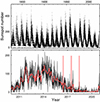 |
Fig. 1. 200-yr span of sunspot numbers places current observations in a wider perspective (top). Around activity minima, days without reported sunspots are not unusual. Recent Cycle 24 with daily sunspot numbers (bottom) from WDC-SILSO (World Data Center – Sunspot Index and Long-term Solar Observations, Royal Observatory of Belgium, Brussels). Superposed red curve shows monthly averages. The selected periods from which HARPS-N data were analyzed are marked with vertical bars. |
3.2. Previous analyses of HARPS-N full-disk solar data
This sequence of solar data has been scrutinized by the HARPS-N team itself. Collier Cameron et al. (2019) carried out a thorough analysis using cross-correlation functions (CCF). Sources of velocity excursions were identified, concluding that for timescales below a day, the granulation signal dominates, with a half-life of 15 min. On longer time-scales, magnetic activity dominates, with active-region passages shifting the apparent radial velocity by several m s−1, accompanied by spectral-line asymmetries that are shifted in time relative to the velocity signal. Long-term trends in the approach to solar minimum appear as slowly changing parameters of the CCF, mirroring a decline in sunspot number and possibly tracing the evolving magnetic network. With a weakened network, an apparent decrease in effective temperature could result (Ludwig et al. 2023; Vögler 2005). Sunspot disk passages trigger peaks in the CCF FWHM while the CCF bisector signature of line asymmetry remains for longer, tracing inhibition of convection in active-region faculae.
The detectability of synthetic planetary signals in HARPS-N solar data was tested by Collier Cameron et al. (2021) and Langellier et al. (2021), suggesting that while improved models of stellar variability will be required, detailed analyses of various correlation functions should be able to segregate stellar magnetic activity. The inverse problem, namely, synthesizing a full-disk signature from modeled granulation was considered by Cegla et al. (2019) and Palumbo et al. (2022). In another study based on these years of observations, Maldonado et al. (2019) studied Ca II H & K, Balmer lines, Na I D1 & D2, and He I D3, finding that activity indices defined in bandpasses around Hα, Hβ, and Hγ lines are anti-correlated with the Ca II S-index. Also from HARPS-N solar spectra, Thompson et al. (2020) further explored activity-related spectral variations.
4. Selecting subsets of HARPS-N solar data
Both the past Kitt Peak survey, our modeling in Paper I, and the results by Maldonado et al. (2019) indicate that a somewhat different behavior among various classes of spectral lines is to be expected but variations are likely to be tiny, that is, possibly at (or beyond) the detection limit. A detailed analysis of the entire large HARPS-N data set was not seen as practical and considerations were taken to select realistically limited subsamples of the best data available.
4.1. Comparing HARPS-N to solar spectrum atlases
First, a sample of 100 spectra was examined to understand more about the character of likely noise sources. We considered how extensive averaging of successive exposures that is feasible without hitting systematic effects. This depends on the extent to which its noise is random in character, such that stacking of spectra decreases the noise in a stable manner. To verify such behavior, traces of the reduced HARPS-N spectra were compared to high-fidelity spectrum atlases of integrated sunlight (Kurucz et al. 1984; Reiners et al. 2016), confirming that the spectra appear to be very stable and that their averaging over multiple exposures indeed shows a stable convergence. However, the continuum levels of the HARPS-N spectra are not normalized over broader spectral regions and (on some accuracy level) the comparison to spectral atlases may start to show physical differences between spectra recorded at different epochs of the solar activity cycle or at different times of year. [Bi]annual variations of the apparent solar rotational velocity are caused by two effects: with the Earth’s orbital plane inclined relative to the solar equator, the rotating Sun is viewed from slightly different angles during the year. The Earth’s prograde orbit is somewhat eccentric, with our orbital angular velocity greater near perihelium, when the velocity vector more closely tracks the sense of the solar rotation, and the apparent solar angular velocity thus decreases. Although small, these effects are seen in HARPS-N data as [bi]annual modulations of spectral-line widths (Collier Cameron et al. 2019).
In the lowest-noise spectral orders, a nominal S/N of ∼400 can be reached in the continuum for each data point with stepsize of 0.82 km s−1 (Fig. 2). One spectral line of medium strength may cover some 25 such points and a selection of ten similar lines, averaged over ten recordings spanning one hour (and if affected by random noise only) could then in principle reach S/N values in excess of 10 000 (even in absorption lines well below the continuum). In reality, however, approaching such precision would require extremely precise control of all other noise sources. One of the aims of the current project is to try to understand how far the search for spectral microvariability can be pushed with existing instruments before being overtaken by systematics.
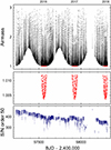 |
Fig. 2. HARPS-N observations of the Sun (top) with each exposure marked by a point (Dumusque et al. 2021). Selected exposures at the smallest airmasses (red points) occurred around daily noon during the summer seasons of 2016–2017–2018. Airmasses for the 1000 selected recordings (middle). S/N values remaining very high, but decreasing slightly over time (bottom), apparently due to diminishing telescope and instrument transmission. |
4.2. Criteria for selecting spectral exposures
Since a detailed analysis of all available data was not seen as practical, some subset of spectral exposures had to be selected. Various criteria were considered: with respect to the level of solar activity, with a uniform sampling in time, of highest S/N values, amongst others. It was concluded that one limiting source of non-random noise likely could be the varying amount of atmospheric telluric absorption. Even if the strongest water vapor lines in the yellow and red spectral regions perhaps could be avoided, micro-tellurics exist throughout the spectrum, contributing noise beyond the random photometric component. The effects of telluric absorption and various methods to remove them have been discussed by numerous authors, such as Artigau et al. (2014), Cunha et al. (2014), Ivanova et al. (2023), Kjærsgaard et al. (2023), Lisogorskyi et al. (2019), Smette et al. (2015), Xuesong Wang et al. (2019), and references therein. Some authors have also concluded that observations from outside the atmosphere will ultimately be required for exoEarth detection (Plavchan et al. 2019). For the present study, to minimize both the amount of tellurics and their variation between exposures, it was decided to select exposures from the smallest airmasses only, implying summertime observations around daily noon (for the La Palma latitude, this also implies approaching close to zenith). The full HARPS-N set of 34 550 spectra includes recordings at also large airmasses Z up to almost 3.1; ∼8600 are at Z < 1.1 and some 2200 are below Z = 1.02.
A total of 1200 exposures with the smallest airmasses were first retrieved from the dataset. From this group, the 1000 apparently best spectra were selected, removing those with the lowest S/N values during each observing season. On some days, significant decreases in the S/N were noted (Fig. 2), which in independent meteorological records could be identified as likely due to the “calima” phenomenon, when the atmospheric transparency above La Palma is diminished by airborne dust from the Sahara. However, that should not generate sharp spectral lines (as opposed to telluric lines at larger airmasses). The final sample of 1000 spectra covers Z = 1.0036 − 1.0120, and originates from the dates May 20 – July 18, 2016; May 19 – July 23, 2017; and May 19 – July 15, 2018. For the selected samples, Fig. 2 shows the airmass distribution over time, and the corresponding S/N for the échelle order nr. 50, as listed in the data set. The S/N values for the selected spectra hover around 400 during the 2016 and 2017 seasons, and around 350 in 2018. The decreasing solar activity during this period is seen as both a decrease in the Mt.Wilson Ca II H & K S-index, as well as a gradually more negative apparent radial velocity, reflecting the smaller area coverage of plages with magnetically disturbed granulation with their locally smaller convective blueshifts (Meunier 2021). Figure 3 shows the overall trend over the years.
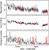 |
Fig. 3. Apparent solar radial velocity (top) growing more negative with time (given as Barycentric Julian Date), apparently due to less magnetic granulation and a smaller suppression of convective blueshift. Mt.Wilson Ca II H & K S-index reflects the slowly declining activity level in the solar cycle (middle) modulated by solar rotation. Daily sunspot numbers from WDC-SILSO (bottom). The periods from which HARPS-N data were analyzed are marked in red or shaded in color. |
In the absence of an absolute reference, the identification of noise sources at the precision limit can be awkward. Tests for consistency were carried out by examining the stability of the supposedly stable pseudocontinua. This identified a period of a few weeks in 2018 with enhanced fluctuations, of unknown origin (simultaneously seen in different spectral regions, as described in Appendix A). As a precautionary measure, all data from those weeks were removed from further analysis.
4.3. Selection of spectral lines
Spectral line categories that are to be selected should be plausible candidates for identifying solar microvariability, probing different sections of the photosphere, and subject to conditions of formation that can likely be modeled. Chromosperic lines, in particular Ca II H & K, were of course monitored since long ago; in several other lines, activity indices have been seen to be correlated with them. Thompson et al. (2020) used HARPS-N spectra to compare epochs of high and low solar magnetic activity, finding that the depths of some spectral lines significantly correlate with the Ca II H & K emission. Related phenomena are seen for chromospherically more active K-type stars. There, Thompson et al. (2017) and Wise et al. (2018) examined HARPS spectra to identify activity indicators that correlate with Ca II, extended by Wise et al. (2022) by carrying out some stellar atmospheric modeling. Identifying the spectral contributions from various solar surface features, Cretignier et al. (2024) concluded that the temporal variations of the Ca II index typically come about 70% from plages, 26% from network, and 4% from spots. In an analogous vein, the main contributions to jittering in radial velocities are found to be the suppression of convective blueshift, not the presence of sunspots (Haywood et al. 2016; Lakeland et al. 2024; Meunier et al. 2010; Sen & Rajaguru 2023).
Photospheric activity measures related to radial velocities were searched for by Davis et al. (2017). They used simulated disk-integrated time-series spectra to demonstrate that different absorption lines respond to activity in non-uniform ways; therefore, averaging over numerous different lines will necessarily wash out the information. They also show that a higher spectral resolution better retrieves information content from spectra that have been affected by stellar activity, improving the distinction among activity and planetary signals.
The line selection should allow us to examine primarily photospheric quantities, ideally in a way that would not be strongly correlated with the classic parameter of Ca II H & K – and thereby carrying independent information. While chromospheric indices do outline the solar activity cycle and also reflect the overall changes of the average solar radial velocity from month to month, their detailed correlation with radial-velocity fluctuations breaks down on levels of m s−1 (Fig. 3), for which some other measures plausibly could exist to serve as proxies. Below, we describe the motivations for the selection of lines from different species, together with discussions of what types of atmospheric phenomena that likely would be sampled by them.
4.4. Selection of line parameters
The choice of parameters that are to be measured is influenced by both the spectrometer performance and by aspects that could be amenable to later theoretical simulations. For example, the modeling in Paper I found that the jittering in radial velocity, as driven by fluctuations in granular convection, differs somewhat in amplitude between lines of different strength and in different wavelength regions. However, the noise levels in present spectra do not allow for the identification of such differential radial-velocity signatures, especially not for limited subsets of selected lines. Realistically measurable parameters, in which tiny variations are also likely to be seen, include the basic line properties of strength, depth, and width. Among these, the absorption equivalent width appears to be the most stable quantity for both observation and theory. Any theoretically modeled line-depth would need to be adjusted not only for solar rotation, but also for the finite spectrometer resolution (Fig. 4); in addition, any fluctuations in width would need to be verified against instrumental profile stability. The equivalent width is (at least to a first approximation) insensitive to minor variations in instrumental profile, even if its exact value depends on the level of spectrometer straylight and on how the continuum level is set. Likewise, the small [bi]annual modulation of the solar spectrum caused by the Earth’s orbital motion should be negligible at the expected precision levels. Only the relative changes in equivalent width would be of significance since absolute line strengths cannot theoretically be very precisely computed, as they are dependent on incompletely known laboratory oscillator strengths and the exact computational treatments of radiative transfer.
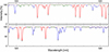 |
Fig. 4. Example of HARPS-N spectra and selection of regions for measurement. Background thin black line: Göttingen solar flux atlas (Reiners et al. 2016). Its higher spectral resolution is evident from its deeper line profiles. Blue line: Average over 100 HARPS-N exposures. Red line: Selected regions of Fe I line absorption. Green line: Selected reference regions of quasi-continua. Thin brown line around 100%: ratio between one representative HARPS-N exposure and a 100-exposure average, illustrating the random-noise level for a single exposure with nominal S/N in grating order 50 equal to 430. The wavelength scale represents values in air (vacuum values in the Göttingen atlas were converted to those in standard air). |
Foreseeing future hydrodynamic 3D modeling, the spectral features should be tightly defined in terms of wavelength. In order to minimize noise from possible wavelength displacements in synthetic spectra, measurements of absorption equivalent widths are made between points in the spectrum with a minimal gradient, occasionally measuring over adjacent similar lines and avoiding measurement boundaries in blends (Figs. 4 and 5). While such a truncation would perhaps not be necessary for spectra from steadily calibrated radial-velocity spectrometers, it might be an issue for synthetic spectra, where spectral-line wavelength errors from laboratory measurements may be no longer negligible. Line absorption is measured relative to the chosen pseudocontinuum segments; of course, they do not reach the exact continuum level, but for measurements of relative variability, that slight difference is not a concern.
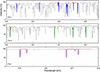 |
Fig. 5. Example of Fe I line selections in shortward parts of the spectrum (blue), of Fe II (green), and of Fe I at long wavelengths (dark purple). Absorption features are truncated at places of small intensity gradients, occasionally embracing several lines. Intermingled pseudocontinua, whose averages are used as an intensity reference, are marked in red. |
There is no precisely stable continuum fitting available that would be feasible over broader spectral regions spanning different échelle orders, recorded during days of possibly variable and chromatic atmospheric extinction. To obtain continuum levels relative to which absorption lines are measured, multiple segments of pseudocontinua were selected. As far as possible, these are chosen close to (and symmetric in wavelength about) the lines to be measured (Figs. 4, 5, 7, 11, 14, and 16). Compromises need to be made how clean these segments can be chosen, considering the need to span many pixels to limit photometric random noise and also to be close to the target line to limit possible systematic drifts.
5. Photospheric Fe I and Fe II lines
Overall, Fe lines are ubiquitous throughout the spectrum and are commonly used for various atmospheric diagnostics, velocity shifts, and other aspects. As listed in Table B.1, Fe I and Fe II line features were selected from various parts of the spectrum, sometimes spanning over multiple lines (Fig. 4). The line selection is essentially the same as used in the theoretical modeling of Paper I, however, with slight differences caused by the lower spectral resolution here, as compared to the synthetic hyper-high one. The lines are grouped as: Fe I 430–445, Fe I 520–535, Fe I 670–685, and Fe II 435–475 nm. These four line groups represent different classes of Fe lines, as was also seen from their dissimilar radial-velocity behavior in Paper I. The drifts in their absorption strength are shown in Fig. 6, plotted as a function of the chromospheric Ca II activity index and the radial velocity. These are parameters that also aptly discriminate between the changes from year to year. Here, as well in later figures, the values in each line group are normalized to 100% of the arithmetic average for their full three-year dataset.
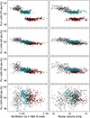 |
Fig. 6. Relative changes of Fe I and Fe II absorption line equivalent widths during the measured periods in 2016 (red), 2017 (cyan), and 2018 (gray). Left column shows the dependence on the Mt.Wilson Ca II H & K chromospheric activity S-index; right column on the radial velocity as obtained from the full HARPS-N spectrum. A lower S/N in the grating orders housing weaker lines at the longest wavelengths accounts for a greater spread of points in the bottom frames. The lines included in each group are listed in Table B.1. |
Similar to the radial-velocity jittering in Paper I, the greatest amplitudes are seen for the Fe II lines at short wavelengths, decreasing for Fe I and at longer wavelengths. With increasing magnetic activity, the line absorption becomes weaker (although the noisier data for the reddest lines are somewhat inconclusive). When plotted against radial velocity, the patterns remain basically similar, although now with a somewhat greater dispersion.
6. Green Mg I triplet and Mg Iλ 457.1 nm
A group of strong lines with formation in the higher photosphere (with contributions from also the lower chromosphere) is the green magnesium triplet of Mg I b1λ 518.3, Mg I b2λ 517.2, and Mg I b3λ 516.7 nm (Fig. 7). Their atomic energy levels are coupled such that they are transitions between one common upper level and three different lower levels with the quantum numbers J = 2, J = 1, and J = 0 for b1, b2, and b3, respectively. Their Grotrian term energy diagram is shown in Alexeeva et al. (2018) and Peralta et al. (2022), for example. Another tantalizing target is the intercombination line Mg Iλ 457.1 nm. Its upper energy level is the same as the lower level of the Mg I b2 line, from where it transits to the ground level. The selected wavelength intervals are in Table B.2.
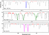 |
Fig. 7. Top: Selected portion of the Mg I 457.1 nm absorption line and its surrounding continuum reference segments (red). Center: Selection of the Mg I b line triplet lines and their continuum reference segments. Bottom: Na I D2 and D1 lines and their continuum segments. |
6.1. Mg I b triplet
The formation of the Mg I b-line triplet in the Sun and in other stars has been discussed by multiple authors. Their line wings probe the upper photosphere while the line cores form in the lower chromosphere. Their shared upper energy level contributes to the complexity of their formation. Since both source functions and opacities are affected by deviations from LTE, local thermodynamic equilibrium (mainly through photoionization), these lines are not particularly sensitive to the local atmospheric structure (Sasso et al. 2017; Zhao et al. 1998). However, the triplet can be seen as a diagnostic for stellar activity (Sasso et al. 2017) and was studied for photospheric changes in G- and K-type stars by Basri et al. (1989). Observed and simulated solar surface images in Mg I b2, with its line formation within photospheric granulation, were evaluated by Rutten et al. (2011). Various aspects of Mg I lines in the Sun and cool stars, including effects of departures from LTE, have been further discussed by Alexeeva et al. (2018), Carlsson et al. (1992), Osorio & Barklem (2016), Peralta et al. (2022, 2023), Sasso et al. (2017), Zhao et al. (1998), and others.
6.2. Intercombination line Mg I 457.1 nm
This rather special, so-called “semi-forbidden,” intersystem line originates between the atomic levels 3s21S0 – 3p 3P1. As compared to the Mg I b triplet, its formation is expected to be relatively simple. Already very early non-LTE calculations showed it to be completely dominated by thermal excitation (e.g., Altrock & Canfield 1974; Altrock & Cannon 1972; Mauas et al. 1988). Due to the dominance of collisional processes in forbidden lines, its source function is tightly coupled to the local temperature. In one-dimensional (1D) model atmospheres, the line forms at around 500 km height and thus provides temperature diagnostics from around the temperature minimum; however, some non-LTE effects could still be present (Langangen & Carlsson 2009; Sasso et al. 2017). At the solar disk center, its lack of a central reversal constrains the lowest possible position of the chromospheric temperature rise, while Carlsson et al. (1992) pointed out that it is the only line in the optical spectrum producing a line center emission reversal at the solar limb (where the line of sight crosses the temperature minimum). Despite its modest atomic oscillator strength, the absorption line is rather strong because its opacity is determined by the relatively high population of its lower energy level – the Mg I ground state.
6.3. Relations among Mg I lines
Figure 8 shows the dependences of Mg I line absorptions as function of the Ca II chromospheric index, and Fig. 9 as function of the radial velocity. The trends among the three Mg I b lines are distinctly different and nor do they follow the Ca II index (however, their behavior is reminiscent of those of the three Balmer lines discussed later in this work). The line strengths vary between the observing seasons, with an anticorrelation between the strongest b1 line, and the two others. The relative changes among the lines show clear and systematic patterns (Fig. 10), with the steepest mutual dependence between b2 and b3. Although it may appear striking on the plots, the total amplitudes amount to only about half a percent in absorption equivalent widths.
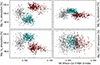 |
Fig. 8. Relative absorption equivalent width changes in Mg I lines during the selected seasons of 2016–2017–2018 (red–cyan–gray), as function of the Mt.Wilson Ca II H & K S-index. |
The data for the weaker Mg Iλ 457.1 nm line are noisier (reflecting its narrower width; Fig. 7) and show no change between the years (Figs. 8 and 9). This special line does not show any correlation with the contemporaneous Mg I b strengths (Fig. 10) and this semi-forbidden line thus appears to be in a class by itself.
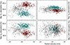 |
Fig. 9. Relative absorption equivalent width changes in Mg I lines during the selected observing seasons of 2016–2017–2018 (red–cyan–gray), as function of the radial velocity for the full spectrum. |
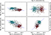 |
Fig. 10. Relative changes in the absorption equivalent widths of the various Mg I lines during the selected seasons of 2016–2017–2018 (red–cyan–gray). Dotted blue lines are fits to the data. |
7. Magnetically influenced features
7.1. The G-band
The G-band is a heavily blended region around 430 nm, with many rotational and vibrational transitions from the CH molecular bandhead, intermingled with numerous atomic lines. Its spectral appearance was described in Paper I in the context of its modeling in non-magnetic and magnetic granulation.
Much of the small-scale magnetic fields outside sunspots is outlined by the bright network. At high spatial resolution, it resolves into solar filigree (sometimes called bright points, although not really point-like), occupying part of the spaces between granules. The corresponding appearance in the chromosphere is more smeared out, apparently reflecting the expansion of magnetic flux into higher layers. Given that convective blueshift is suppressed in magnetically disturbed granulation and because of their large areal extent (also far outside sunspot groups), it has been found that the changing area coverage of the magnetic network and its associated plages is responsible for a great fraction of the solar-cycle modulation in apparent radial velocity, quantitatively confirmed by Lakeland et al. (2024) and Meunier et al. (2010).
The magnetic network of the quiet Sun appears bright in various spectral regions, in particular in molecular and other temperature-sensitive lines. Among these, observations and modeling in the G-band are particularly extensive (Paper I). Since the G-band emission thus traces the network, it appears plausible that the G-band brightness could be a proxy for the magnetic network in integrated sunlight.
Figure 11 shows the G-band spectrum, as measured by HARPS-N. The adopted boundaries are the same as in the synthetic spectra at hyper-high resolution in Paper I, with the full G-band spanning 429.84–431.33 nm, and its central core 430.71–430.88 nm (Table B.2). Also, the ten nearby Fe I lines (Table B.1) and the 32 pseudocontinuum reference points are identical. A comparison with Fig. 12 in Paper I demonstrates effects of different spectral resolutions.
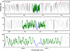 |
Fig. 11. G-band region together with selected spectral features as observed with HARPS-N: G-band core (dotted blue), full G-band (dotted blue + green), surrounding nearby Fe I lines (black), and pseudocontinuum reference points (red). An averaged 100-exposure spectrum is plotted in thin gray. From top down, successively narrower spectral segments are shown. |
The absorption in these bands is shown in Fig. 12. Over the years, the systematic changes in both the full G-band, and in its core are quite similar to those in Mg I b1, the strongest line of the triplet, but differ from those in the weaker Mg I b lines (Fig. 8). The nearby Fe I lines that crowd around the G-band strengthen with increased magnetic activity, a trend opposite to that for the more isolated photospheric Fe I lines seen in Fig. 6.
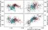 |
Fig. 12. Absorption equivalent widths for the full G-band region, its central core, and nearby Fe I lines, as function of the Ca II H & K S-index. The different seasons of 2016, 2017, and 2018 are marked in red, cyan, and gray. Also, the corresponding radial velocity variations for the full spectrum are shown. For cases with apparent systematic dependences, dotted blue lines show fitted relations. |
The flux in the G-band core is more variable than that of the full G-band. As examined in Paper I, the core has enhanced sensitivity to both spatial and magnetic variations, and such a variability difference is thus expected. Figure 13 shows the measured G-band quantities both as absorption and as flux, the latter corresponding to what is observed in monochromatic solar images. Similar to the dependence for Ca II H & K, there is a correlation with simultaneous variations in radial velocity, although the relation shows more scatter (Figs. 12 and 13).
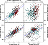 |
Fig. 13. Ratios between the full G-band fluxes and its absorption equivalent widths, the G-band core, and that of nearby Fe I lines. Different seasons of 2016, 2017, and 2018 are marked in red, cyan, and gray. Fitted relations are dotted blue lines, while the identity relations are dashed black. The core flux shows a steeper relative variability than the full band. |
Enhanced contrast in magnetic fluxtubes is produced also in other spectral features, in particular molecular lines. As remarked in Paper I, the violet CN band around 388 nm gives a contrast about 1.4 times greater than the G-band; however, observationally that short-wavelength region is more demanding (and also falls shortward of the HARPS-N spectral range). Signatures from CN should represent the low chromosphere. A narrow feature of the CN 388.3 nm bandhead was included in the Kitt Peak monitoring program, showing a full solar-cycle peak-to-peak amplitude of ∼3% (Livingston et al. 2007) that is an order of magnitude smaller than the corresponding change in the Ca II H & K index.
7.2. Hyperfine split Mn Iλ 539.47 nm
Another class of lines that may carry particular signatures from photospheric magnetic regions are those whose atomic structure causes hyperfine splitting. This causes broad, intrinsically wide, and flat-bottomed profiles, for which the line broadening is quite insensitive to nonthermal motions such as the wavelength smearing by granular velocities. This makes them suitable as temperature indicators, a property examined previously by Elste & Teske (1978), Elste (1986), Erkapić & Vince (1993), and Vince & Vince (2003).
A prominent line is Mn Iλ 539.47 nm, with a hyperfine broadening comparable to its thermal one. At Kitt Peak, its measurement in integrated sunlight began in 1979. It turned out to vary differently from other features, showing the greatest solar-cycle variation (Livingston et al. 2007; Livingston & Wallace 1987). Its equivalent width was measured to change from about 7.86 pm at solar activity maximum to about 7.98 pm at minimum, an amplitude of ∼1.5%. This line was later included in a full-disk monitoring program in Belgrade (Arsenijević et al. 1988; Vince et al. 1988), confirming the solar-cycle amplitude (Danilović & Vince 2004; Danilović et al. 2005; Skuljan et al. 1992, 1993).
Suggested explanations included optical pumping from the ultraviolet Mg II k λ 279.55 nm that happens to almost coincide with a transition in Mn (Doyle et al. 2001), but later analyses by Danilovic et al. (2016) and Vitas & Vince (2005, 2007) showed that this is not significant. However, the temperature sensitivity of this Mn I line causes its absorption to weaken less in normal granulation and monochromatic images therefore show a bright network, similar to an unsigned magnetogram (Malanushenko et al. 2004; Vince et al. 2005). That its line parameters stand out in contrast to nearby Fe I lines is seen also in solar spectra from the center to the limb (Osipov & Vasilyeva 2019), while the solar-cycle variations can be modeled with changing distributions of solar magnetic features (Danilovic & Vince 2005; Danilovic et al. 2016). As opposed to other lines often used in solar magnetometry, Mn Iλ 539.47 nm weakens with increasing field strength, making it sensitive to weaker fields in the quiet Sun as well (López Ariste et al. 2002; Sánchez Almeida et al. 2008; Vitas et al. 2009).
Its behavior was further clarified in 3D modeling and spectral synthesis by Vitas et al. (2009). The line weakens in intergranular magnetic concentrations; meanwhile, the corresponding effect in ordinary and narrower photospheric lines has less of an impact in full-disk flux due to their decreased line depth in normal granulation. Somewhat analogous effects exist for the G-band, and in the extended wings of strong lines such as Hα or Hβ (Leenaarts et al. 2006a,b; Leenaarts & Carlsson 2012). For other late-type stars, 3D non-LTE calculations for Mn I are by Bergemann et al. (2019). As compared to Fe, Mn is particularly sensitive to non-LTE effects because of a low cosmic abundance, great photo-ionisation cross-sections, and a somewhat special atomic energy level structure.
The extent to which the Mn Iλ 539.47 nm could be affected by telluric absorption was examined by Vince & Vince (2010). Its core was found to be free from such contamination although tellurics might affect unsuitably chosen local continuum regions.
7.3. Other hyperfine split Mn I lines
Given this behavior, the detailed variability in lines such as Mn Iλ 539.47 nm might well carry specific signatures about photospheric magnetic conditions connected to also radial-velocity fluctuations. In the case of our HARPS-N data, an issue arises as to how small fluctuations reliably can be measured. If guided by previous Kitt Peak and Belgrade measurements, the change over our current fraction of a solar activity cycle can be expected to be only a fraction of one percent. As it is not especially strong (Fig. 14), the line extends over only a limited wavelength range and the noise level makes it hard to deduce a likely physical signal, as seen on the top row of Fig. 15.
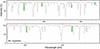 |
Fig. 14. Examples of selected Mn I lines with hyperfine splitting in the 540 nm region with pseudocontinuum segments marked in red. The lines are noticeably broader than others of comparable depth. The full set of sampled Mn I lines extends over the range 511–644 nm (Table B.2). |
Some other lines were considered as candidates for measurement but, although also a few other atomic species display hyperfine structure, those from Mn I are the most distinct. López Ariste et al. (2002) list Mn I lines with conspicuous broadenings related to their hyperfine structure. Of their 19 lines, 16 fall within the HARPS-N spectral range and were chosen to represent a more general hyperfine splitting signature (Table B.2). Their equivalent widths were measured individually relative to pseudocontinua around each of them and their summed equivalent width of about 80 pm (800 mÅ) is shown on the bottom row of Fig. 15.
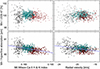 |
Fig. 15. Variations in hyperfine split Mn I lines. Data for the previously studied single line λ 539.47 nm (top row) are inconclusive but the summed equivalent widths of 16 different Mn I lines reveal a clear trend (bottom). Data for 2016–2017–2018 are shown in red–cyan–gray. |
The signal summed from these 16 lines now shows a clear trend during 2016–2017–2018 as an increase in the absorption by ∼0.3% when going toward years of lower solar activity. This is consistent with the trends seen earlier at Kitt Peak and Belgrade for their single line. However, perhaps contrary to expectations, the trends are qualitatively similar and actually smaller compared to what was seen for more ordinary Fe I and Fe II lines in Fig. 6.
7.4. Unsigned magnetic flux and line formation
The variability of several spectral lines is influenced by the (unsigned) magnetic flux (Rutten 2019). That can be measured from (unpolarized) intensity spectra by fitting the line-broadening dependence among lines with known Landé geff-factors for magnetic sensitivity. For HARPS-N solar spectra, this was done by Lienhard et al. (2023), averaging over more than 4000 lines. With sufficient S/N, one would be able to examine lines with different Zeeman sensitivity and formed in different (and also differently moving) photospheric structures (e.g., Liu et al. 2023). Line pairs with different Zeeman sensitivities but otherwise similar properties and formed under the same atmospheric conditions could provide more precise determinations (Smitha & Solanki 2017).
Magnetic fields in the quiet Sun have been reviewed by Bellot Rubio & Orozco Suárez (2019) and (Sánchez Almeida & Martínez González (2011). Different spectral lines have different sensitivities to differently strong magnetic fields (Quintero Noda et al. 2021), while near-infrared lines might be especially valuable for mapping fields into the deeper photosphere (Hahlin et al. 2023; Lagg et al. 2016). Thus, there exists a wealth of information about spectral-line properties in solar magnetic structures; however, not much of this can yet be utilized for the Sun-as-a-star because of limiting S/N and finite spectral resolution in even the best current radial-velocity instruments.
8. The strongest lines
Although we are mainly focused here on photospheric features, some stronger and more chromospheric lines are also considered. They may not provide precise radial velocities, but their measurements are tied to previous works for Ca II H & K, they display greater variability than purely photospheric lines, and they are useful as indicators for magnetic activity.
We generally reference various measures to the Mt.Wilson S-index for Ca II H & K (Fig. 3), obtained as the flux in the central (chromospheric) emission core, relative to that in the (mainly photospheric) flanks of the absorption lines. This quantity was examined by Egeland et al. (2017) while the definition (Duncan et al. 1991) goes back to the specifics of the Mt.Wilson coudé spectrograph (Vaughan et al. 1978), later calibrated on also other spectrometers (Hartmann et al. 1984; Oranje 1983). The Ca II emission has been studied by many; its solar-cycle variation by White & Livingston (1981) and line profiles in solar plages by Oranje (1983). Dumusque et al. (2021) described it for HARPS-N spectra and the values in our plots are from its data release. Line components in solar surface structures were examined by Cretignier et al. (2024) and long-term variations by Singh et al. (2023). On the smallest scales, bright grains appear to be produced by shocks in the mid-chromosphere (Carlsson & Stein 1997; Van Kooten & Cranmer 2024).
For the appearance of Ca II H & K in stars very similar to the Sun, we refer to Pasquini et al. (1988) for α Cen A (G2 V) and Dravins et al. (1993) for β Hyi (G2 IV). A broader review of stellar chromospheric variability is offered in de Grijs & Kamath (2021).
8.1. Balmer lines: H α, H β, H γ
Also Hα can be used to indicate stellar activity. Over solar active regions, its absorption core is partially filled in, and its flux is thus affected by chromospheric activity. In G- and K-dwarfs and subgiants, this was considered by Cayrel et al. (1983), Cincunegui et al. (2007), Gomes da Silva et al. (2014, 2022), Martínez-Arnáiz et al. (2010), Pasquini & Pallavicini (1991), Zarro (1983), Zarro & Rodgers (1983), and others. The approach is more practical for active stars, where the filling-in is greater than the sub-percent values for integrated sunlight. From an extensive sample of F, G, and K stars observed with HARPS, Gomes da Silva et al. (2022) studied how the signals depend on the chosen bandwidths for the flux, and how that varies with stellar activity level and metallicity. Bandpass choices with a narrow central interval referenced to surrounding broader regions are mainly oriented toward an expected narrow central emissions in more active stars (Boisse et al. 2009; Bonfils et al. 2007; Kürster et al. 2003).
The Hα transition has its lower energy level at 10.2 eV, which means that the line opacity is quite temperature-dependent. Because of hydrogen’s low atomic weight, its thermal broadening is very large and the line is not a good diagnostic of nonthermal motions. The line width is instead a measure of the gas temperature and the core intensity of its formation height; greater height means lower intensity (Cauzzi et al. 2009; Leenaarts & Carlsson 2012).
The extended shortward wings of Hα or Hβ carry signals of unsigned magnetic fields analogous to Mn I or the G-band (Leenaarts et al. 2006a,b; Leenaarts & Carlsson 2012). These line wings obtain contrast enhancement through a reduction of line opacity in magnetic concentrations with locally lesser damping. However, full-disk spectra face the complication that bright magnetic areas can be dimmed by overlying dark chromospheric filaments. The emergence, passage, and decay of active solar regions induce variability patterns in Balmer lines (Marchenko et al. 2021).
8.2. Balmer-line variability in integrated sunlight
In the Kitt Peak monitoring program, Hα became listed among those lines varying in strength like Ca II, but with lower relative amplitudes. The Hα absorption depth was found to drift from ∼84.0% at activity minimum to become slightly shallower (∼83.5%) at activity maximum, a slight filling-in of the line center; Livingston et al. (2007, 2010), further examined by Meunier & Delfosse (2009).
Balmer lines in the spectrum of the Sun as a star were also evaluated by Criscuoli et al. (2023), using spaceborne radiometers and ground-based spectra. They identified correlations with network, prominences, filaments and others, finding that both the core and wings contribute to the variability, supporting the view that Balmer line core-to-wing ratios behave more like photospheric than chromospheric indices. For different Balmer lines, current HARPS-N data were examined by Maldonado et al. (2019), including the modulation by solar rotation. The very cores of the lines were integrated over 0.16 nm and the wings over about 1 nm. They confirmed certain correlations with the Ca II index, more pronounced at times with greater sunspot numbers.
The Balmer lines display very extended wings that are blended by numerous weaker lines and there is no unique definition of how their precise strengths would be measured. We adopted the absorption over central portions, referenced to nearby pseudocontinuum levels in their far wings, analogous to previous Hα indices, but now covering a wider part of the profiles, where much outside the very cores must be of photospheric origin. Our sampling intervals for Hα and Hβ are thus much broader than those used by Maldonado et al. (2019), and others (Table B.2).
These intervals for Hα, Hβ, and Hγ are shown in Fig. 16, and should also be practical to use in foreseen models of magnetically influenced atmospheres (Paper I was oriented toward metal lines in the photosphere proper, not strong lines in higher layers). For the desired precision, however, telluric lines touching Hα may start to become an issue (Dravins et al. 2015).
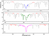 |
Fig. 16. Spectral regions around Hα, Hβ, and Hγ. Solid bold lines denote the line intervals measured; for Hβ its central core was also measured separately (dotted). In each case, lines are measured relative to local pseudocontinua marked in red, chosen symmetrically about the line centers. The average spectrum from 100 HARPS-N exposures is plotted as a thin dark line. The intensities are normalized to each local pseudocontinuum. |
Over the years, there are gradual and systematic changes (Fig. 17), with Hα varying with much greater amplitude than the others. However, the variations change sign between the successive Balmer lines. With increased chromospheric activity, Hα becomes filled-in (as expected) but the Hγ absorption instead strengthens, with Hβ fluctuations somewhat indeterminate in between. This diversity among lines of varying strengths is reminiscent of what is seen among the lines in the Mg I triplet (Fig. 8).
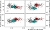 |
Fig. 17. Relative absorption equivalent widths for the Balmer lines Hγ, Hβ (full and core), and Hα, as function of the Mt.Wilson Ca II H & K S-index. Different colors indicate data from the observing seasons of 2016 (red), 2017 (cyan) and 2018 (gray). Because of its greater variability, the vertical scale for Hα is more extended. |
For Hβ, its central and less blended core (Fig. 16) was also measured separately. A comparison shows the Hβ core to be somewhat less variable than the full line; possibly the wings could be affected by dynamic chromospheric events (Fig. 18). We note that the line-center activity indices in Maldonado et al. (2019) showed a positive correlation for changes in Hα, Hβ, and Hγ, but their reference wavelengths are different. Such disparate responses of Balmer and Mg I lines to magnetic regions should become possible to capture with 3D models, once these are made to extend to also higher atmospheric layers than the photosphere proper.
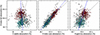 |
Fig. 18. Ratios of the absorption equivalent widths for the Balmer lines Hα, the Hβ core, and Hγ, versus that of the full Hβ (Fig. 16). Red, cyan, and gray indicate data from the observing seasons of 2016, 2017, and 2018. Dashed lines show the identity ratios while those in dotted blue are fits to the data. Because of its greater variability, the horizontal scale for Hα is more extended. |
Especially in the case of Hβ, the relation between line strength and Ca II emission is not clear (Fig. 17). We note that in a fraction of F–G–K stars, complex relationships between Ca II and Hα chromospheric emission have been seen, including clear anticorrelations (Meunier et al. 2022). Besides emission from magnetic plages and network, absorbtion from dark filaments could perhaps be at work (Meunier & Delfosse 2009). Such filaments could be expected to primarily modify the Hα signal, with much smaller effects on the less opaque higher Balmer lines, possibly offering a clue to our anticorrelation between Hα and Hγ.
8.3. Na I D1 and D2 lines
The Na I D1 and D2 are two strong lines used as diagnostics for the upper photosphere and the lower chromosphere (Fig. 7). Usually, the weaker and less blended Na I D1 is used. Monochromatic images across the line profiles reveal the atmospheric structures contributing to the local intensity. The photospheric network is visible in Na I D1 line wings, but largely vanishes in its core, indicating that one is begins to see the top of granulation proper (Rutten et al. 2011). These lines are also used to diagnose exoplanetary atmospheres, but reliable conclusions from the subtle signal then measured differentially to the stellar spectrum, requites a detailed understanding of line formation in 3D and non-LTE (Canocchi et al. 2024). Spatially averaged profiles show a red asymmetry in the core with bisectors in the shape of an inverse C, opposite to that commonly seen in photospheric lines (Uitenbroek 2006). Still, the flux in Na I D1 is largely photospheric. Leenaarts et al. (2010) find that most of its brightness samples the magnetic network in the photosphere, well below chromospheric heights. Similarly to other stronger lines, magnetic bright points are visible also in Na I D1 (Jess et al. 2010; Keys et al. 2013).
The measured absorption in Na I D1 and D2 during the seasons is shown in Fig. 19. Although the amplitudes do not much exceed one percent, the variability is greater than in photospheric lines and merits a closer examination. This spectral region is one affected by telluric lines and (as discussed above), this may start to become the limiting parameter for ground-based observations. An example of heavy telluric contamination in Na I D1 and D2 was shown by Kjærsgaard et al. (2023), comparing different removal algorithms. Although their spectrum (a winter exposure) was carried out through airmasses and water vapor levels much higher than ours, they illustrate the perils at these wavelengths.
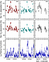 |
Fig. 19. Relative variations of the measured Na I D1 and D2 absorption during the seasons of observation. Bottom: Precipitable water vapor above the Roque de los Muchachos observatory on La Palma. Time is given as Barycentric Julian Date. Spectral data from the noisier period in 2018 are omitted (Fig. A.1). |
Figure 19 also shows the precipitable water vapor during our data periods, as measured above the Roque de los Muchachos observatory on La Palma. Those atmospheric measurements (Castro-Almazán et al. 2016) are routinely carried out using GPS instrumentation. Daily variations can be seen to correlate with apparent changes in line parameters, with times of enhanced water content often coinciding with increased line absorption. Clearly, such fluctuations in Na I D1 and D2 do not reflect solar microvariability but rather provide an example of the limits for measurements without detailed modeling of telluric absorption, even for summer observations close to zenith. No correlations with water vapor were seen for any other among our lines.
With a reservation for possible differential telluric effects, Fig. 20 shows the differential variability between Na I D1 and D2. The amplitudes are greater for the weaker D1, which seemingly has more room to strengthen than the more saturated D2, also seen in the dependence on the Ca II H & K S-index.
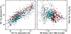 |
Fig. 20. Differential variability of absorption in Na I D1 and D2 lines. The observing seasons of 2016, 2017, and 2018 are marked in red, cyan, and gray. The identity relation is dashed while linear fits are dotted blue. The weaker Na I D1 line is more variable than the more saturated D2, while their ratio mirrors the chromospheric activity index. |
8.4. Lines in the near infrared
The infrared Ca triplet lines at λ 849.8, λ 854.2, and λ 866.2 nm reflect activity in stars (Busà et al. 2007; Foing et al. 1989; Huang et al. 2023), while their synthetic spectra and issues of telluric line contamination are considered by Chmielewski (2000). A comparison between this triplet and Ca II H & K is by Martin et al. (2017). However, these lines fall longward of the HARPS-N spectral range.
Further into the infrared, the He Iλ 1083 nm variability in the Sun as a star was studied by Harvey (1984), Li & Feng (2020), Shcherbakov & Shcherbakova (1991), and Shcherbakov et al. (1996). Another helium line, He I D3, carries chromospheric signatures in main-sequence stars (Danks & Lambert 1985). In integrated sunlight, such lines are being observed with the NIRPS3 spectrometer at ESO on La Silla (Wildi et al. 2022), but the precision is challenged by the need to accurately reduce for the enhanced telluric absorption in the infrared.
9. Spatially resolved solar activity
Any variations in integrated sunlight originate from changes in solar surface structures. Among the lines studied here, Hα is likely the only one where a connection with specific surface phenomena can be identified. Even if its fluctuations may largely be chromospheric, its behavior may hint at how also photospheric lines are modulated, even if on some lesser order of magnitude.
Monochromatic Hα images are continuously being recorded by the GONG collaboration (Global Oscillation Network Group 2024), together with magnetic fields, and other. In Fig. 21, we attempt to connect representative Hα variability with surface patterns. For the 2016 summer season, the Hα flux (rather than absorption) within its passband (Fig. 16, Table B.2) is plotted, together with representative full-disk images and magnetograms from particular days exhibiting local flux minima and maxima. An image examination suggests that instances of higher flux often occur (not surprisingly) when there are larger areas of bright plage on the disk and/or large prominences outside the limb. Lower flux seems to be common when central disk regions have no distinct plages, but more often large dark filaments, which is a distinctive signature for Hα (Meunier & Delfosse 2009). However, the correlation of flux levels with magnetic field morphology appears to be weak: although bipolar active regions are shaping the Hα structures, those may be either bright plage or dark filaments, not generating any unique correlations. Such examples demonstrate that fluctuations in the photosphere need to be measured in photospheric lines and, due to the rapid change of physical conditions with height, are unlikely to offer precise proxies in lines formed in higher layers. Of course, Ca II K chromospheric emission correlates well with the magnetic patterns but even magnetograms recorded in photospheric lines may only represent some particular atmospheric layer since their Zeeman signal is derived from the flanks or wings of the line profiles, which are formed at some height where the fields have already expanded somewhat from their deeper photospheric concentrations.
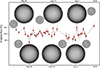 |
Fig. 21. Variations in Hα flux (not absorption) measured during the 2016 data period, together with contemporaneous full-disk Hα images and (adjacent smaller circles) photospheric magnetograms, at selected labeled dates of local Hα-flux maxima or minima. Daily Hα flux averages are large red dots, individual exposures are small and black. The full-disk images were acquired by GONG instruments operated by NISP/NSO/AURA/NSF with contributions from NOAA (Global Oscillation Network Group 2024). |
10. Conclusions and outlook
Besides providing very precise wavelength measurements, the long-term stability of radial-velocity spectrometers enables extreme-precision stellar spectroscopy. In observations of the spectrum of the Sun as a star, its microvariability was measured between successive years, with systematically different amplitudes found among different spectral features. Nonetheless, limitations are that current data cover only part of one single activity cycle (cf. Fig. 1) and the photometric precision limits the signal for individual lines or narrower spectral segments.
A pattern with greater line-strength amplitudes for Fe II lines in the violet follows the theoretically predicted trends in Paper I for short-term jittering in radial velocities. The somewhat stronger lines in the green Mg I triplet show intriguingly variant behavior among themselves, while the semi-forbidden Mg Iλ 457.1 nm appears to be stable. The central parts of the G-band and of Hβ vary with different amplitudes than their full extents. Such examples highlight that the signatures from different lines or line groups carry dissimilar information and need to be considered separately (e.g., Al Moulla et al. 2024; Artigau et al. 2022; Deming et al. 2024, and references in Paper I).
To find proxies with the required precision to mitigate radial-velocity fluctuations toward exoEarth detection, it may well be necessary to understand the detailed physical origin of specific line-profile variability and how variations (in, e.g., equivalent widths) are related to wavelength displacements. Photospheric line changes are seen to correlate with variations in the Ca II H & K index, demonstrating the influence of magnetic fields and motivating spectral modeling of the magnetic photosphere. For different stars, 3D modeling already allows for the synthesis of hyper-high resolution spectra, revealing details in line profile shapes and wavelength shifts among various classes of spectral features (e.g., Dravins et al. 2021a, and Paper I).
However, the spectral resolution of most radial-velocity instruments may not suffice to test or guide such models since line asymmetries and shifts get significantly degraded already at resolutions λ/Δλ ∼ 100 000. It has been argued that resolutions of such order could be optimal if the criterion is to measure wavelength displacements in the flanks of medium-strength spectral lines using a minimal observing time. That of course is relevant for large-scale surveys of numerous stars, where observing time is limited. However, if the priority is to extract the maximum of physical spectral-line information and to identify particularly small signals, other criteria apply.
A resolution of 100 000 (corresponding to 3 km s−1) only provides some three or four independent wavelength points across a typical photospheric line. While this may provide a value for the line strength and indicate its general sense of asymmetry, further details of the line profile are washed out, as demonstrated in numerous works on both observed and synthetic solar spectra (e.g., Dravins et al. 2021b; Löhner-Böttcher et al. 2019). A more satisfying spectral resolution of 270 000, accompanied with a S/N of up to 8000 was realized for the Sun (seen as a star) with the PEPSI4 spectrometer on the LBT5 (Strassmeier et al. 2018). Such numbers would be much preferred for the monitoring of sunlight, as this starts to become adequate to measure actual line shapes. Such S/N also should enable us to identify behavior in individual weaker lines (rather than group averages) and to follow their short-term jittering, segregating from instrumental issues. Some monitoring of the solar flux spectrum has been carried out with PEPSI (Dineva et al. 2020), feeding light via a fiber connection from a small solar-disk integration telescope of 13 mm aperture. A recent upgrade of that telescope has also polarimetric capabilities. An even higher resolution, and with extremely stable wavelengths, could be achieved from a solar-cycle sequence of FTS spectral atlases; however, their specific observing mode and required integration times would not resolve short-term fluctuations (Debus et al. 2023; Reiners et al. 2016).
In the shorter term, a significant improvement should be possible, once the PoET6 solar telescope (Leite et al. 2022) is connected to the ESPRESSO spectrometer of ESO on Paranal (Pepe et al. 2021), enabling sunlight spectroscopy with spectral resolutions of λ/Δλ ∼ 200 000. In the longer term, it should be noted that photon fluxes from brighter stars in larger telescopes are fully adequate to record low-noise spectra also at hyper-high resolutions of λ/Δλ ∼ 1 000 000, for instance. However, the design of corresponding spectrometers remains challenging. If a cross-dispersed échelle remains the design of choice, diffraction-limited adaptive-optics photonic spectrometers will likely be required in order to limit their physical size. Discussions of promising designs are underway (Bechter et al. 2020; Crepp 2014; Jovanovic et al. 2016, 2017; Plavchan et al. 2019) and some of these could serve as appealing alternatives for later-generation instruments on large, very large, and extremely large telescopes.
The 3.5 m Telescopio Nazionale Galileo.
High Accuracy Radial velocity Planet Searcher for the Northern hemisphere.
Near InfraRed Planet Searcher.
Potsdam Echelle Polarimetric and Spectroscopic Instrument.
Large Binocular Telescope.
Paranal solar ESPRESSO Telescope.
Acknowledgments
The work by D.D. is supported by grants from The Royal Physiographic Society of Lund. We thank Julio A. Castro-Almazán and the Sky Quality Team of the Instituto de Astrofísica de Canarias for providing measurements of the precipitable water vapor above the Roque de los Muchachos observatory on La Palma. For the full-disk solar images, this work utilizes GONG data obtained by the NSO Integrated Synoptic Program, managed by the National Solar Observatory, which is operated by the Association of Universities for Research in Astronomy (AURA), Inc. under a cooperative agreement with the National Science Foundation and with contribution from the National Oceanic and Atmospheric Administration. The GONG network of instruments is hosted by the Big Bear Solar Observatory, High Altitude Observatory, Learmonth Solar Observatory, Udaipur Solar Observatory, Instituto de Astrofísica de Canarias, and Cerro Tololo Interamerican Observatory. Parts of this paper were completed by D.D. during a stay as a Scientific Visitor at the European Southern Observatory in Santiago de Chile. Extensive use was made of NASA’s ADS Bibliographic Services and the arXiv® distribution service. We thank the referee for very knowledgeable and detailed comments.
References
- Allart, R., Lovis, C., Faria, J., et al. 2022, A&A, 666, A196 [NASA ADS] [CrossRef] [EDP Sciences] [Google Scholar]
- Al Moulla, K., Dumusque, X., & Cretignier, M. 2024, A&A, 683, A106 [NASA ADS] [CrossRef] [EDP Sciences] [Google Scholar]
- Altrock, R. C., & Cannon, C. J. 1972, Sol. Phys., 26, 21 [NASA ADS] [CrossRef] [Google Scholar]
- Altrock, R. C., & Canfield, R. C. 1974, ApJ, 194, 733 [NASA ADS] [CrossRef] [Google Scholar]
- Arsenijević, J., Kubičela, A., Vince, I., et al. 1988, Bull. Obs. Astron. Belgrade, 138, 1 [Google Scholar]
- Alexeeva, S., Ryabchikova, T., Mashonkina, L., et al. 2018, ApJ, 866, 153 [NASA ADS] [CrossRef] [Google Scholar]
- Artigau, É., Astudillo-Defru, N., Delfosse, X., et al. 2014, Proc. SPIE, 9149, 914905 [NASA ADS] [CrossRef] [Google Scholar]
- Artigau, É., Cadieux, C., Cook, N. J., et al. 2022, AJ, 164, 84 [NASA ADS] [CrossRef] [Google Scholar]
- Baker, A. D., Blake, C. H., & Reiners, A. 2020, ApJS, 247, 24 [Google Scholar]
- Baranne, A., Queloz, D., Mayor, M., et al. 1996, A&AS, 119, 373 [NASA ADS] [CrossRef] [EDP Sciences] [Google Scholar]
- Basri, G., Wilcots, E., & Stout, N. 1989, PASP, 101, 528 [NASA ADS] [CrossRef] [Google Scholar]
- Bechter, A. J., Crass, J., Tesch, J., et al. 2020, PASP, 132, 015001 [NASA ADS] [CrossRef] [Google Scholar]
- Bellot Rubio, L., & Orozco Suárez, D. 2019, Liv. Rev. Solar Phys., 16, 1 [CrossRef] [Google Scholar]
- Bergemann, M., Gallagher, A. J., Eitner, P., et al. 2019, A&A, 631, A80 [NASA ADS] [CrossRef] [EDP Sciences] [Google Scholar]
- Boisse, I., Moutou, C., Vidal-Madjar, A., et al. 2009, A&A, 495, 959 [NASA ADS] [CrossRef] [EDP Sciences] [Google Scholar]
- Bonfils, X., Mayor, M., Delfosse, X., et al. 2007, A&A, 474, 293 [NASA ADS] [CrossRef] [EDP Sciences] [Google Scholar]
- Brandt, P. N., & Solanki, S. K. 1990, A&A, 231, 221 [NASA ADS] [Google Scholar]
- Bruning, D. H., & Labonte, B. 1985, Sol. Phys., 97, 1 [CrossRef] [Google Scholar]
- Busà, I., Aznar Cuadrado, R., Terranegra, L., et al. 2007, A&A, 466, 1089 [NASA ADS] [CrossRef] [EDP Sciences] [Google Scholar]
- Canocchi, G., Lind, K., Lagae, C., et al. 2024, A&A, 683, A242 [NASA ADS] [CrossRef] [EDP Sciences] [Google Scholar]
- Carlsson, M., & Stein, R. F. 1997, ApJ, 481, 500 [Google Scholar]
- Carlsson, M., Rutten, R. J., & Shchukina, N. G. 1992, A&A, 253, 567 [NASA ADS] [Google Scholar]
- Castro-Almazán, J. A., Muñoz-Tuñón, C., García-Lorenzo, B., et al. 2016, Proc. SPIE, 9910, 99100P [CrossRef] [Google Scholar]
- Cauzzi, G., Reardon, K., Rutten, R. J., et al. 2009, A&A, 503, 577 [NASA ADS] [CrossRef] [EDP Sciences] [Google Scholar]
- Cavallini, F., Ceppatelli, G., & Righini, A. 1985, A&A, 143, 116 [NASA ADS] [Google Scholar]
- Cavallini, F., Ceppatelli, G., & Righini, A. 1986, A&A, 158, 275 [NASA ADS] [Google Scholar]
- Cavallini, F., Ceppatelli, G., & Righini, A. 1988, A&A, 205, 278 [NASA ADS] [Google Scholar]
- Cayrel, R., de Strobel, G. C., Campbell, B., et al. 1983, A&A, 123, 89 [NASA ADS] [Google Scholar]
- Cegla, H. M., Watson, C. A., Shelyag, S., et al. 2019, ApJ, 879, 55 [NASA ADS] [CrossRef] [Google Scholar]
- Chatzistergos, T., Krivova, N. A., & Ermolli, I. 2022, Front. Astron. Space Sci., 9, 336 [NASA ADS] [CrossRef] [Google Scholar]
- Chmielewski, Y. 2000, A&A, 353, 666 [NASA ADS] [Google Scholar]
- Cincunegui, C., Díaz, R. F., & Mauas, P. J. D. 2007, A&A, 469, 309 [NASA ADS] [CrossRef] [EDP Sciences] [Google Scholar]
- Claudi, R., Ghedina, A., Pace, E., et al. 2020, Proc. SPIE, 11445, 114452S [Google Scholar]
- Collier Cameron, A., Mortier, A., Phillips, D., et al. 2019, MNRAS, 487, 1082 [Google Scholar]
- Collier Cameron, A., Ford, E. B., Shahaf, S., et al. 2021, MNRAS, 505, 1699 [NASA ADS] [CrossRef] [Google Scholar]
- Cosentino, R., Lovis, C., Pepe, F., et al. 2012, Proc. SPIE, 8446, 84461V [Google Scholar]
- Crass, J., Gaudi, B. S., Leifer, S., et al. 2021, ArXiv e-prints [arXiv:2107.14291] [Google Scholar]
- Crepp, J. R. 2014, Science, 346, 809 [NASA ADS] [CrossRef] [Google Scholar]
- Cretignier, M., Dumusque, X., Hara, N. C., et al. 2021, A&A, 653, A43 [NASA ADS] [CrossRef] [EDP Sciences] [Google Scholar]
- Cretignier, M., Pietrow, A. G. M., & Aigrain, S. 2024, MNRAS, 527, 2940 [Google Scholar]
- Criscuoli, S., Marchenko, S., DeLand, M., et al. 2023, ApJ, 951, 151 [NASA ADS] [CrossRef] [Google Scholar]
- Cunha, D., Santos, N. C., Figueira, P., et al. 2014, A&A, 568, A35 [NASA ADS] [CrossRef] [EDP Sciences] [Google Scholar]
- Danilović, S., & Vince, I. 2004, Serb. Astron. J., 169, 47 [CrossRef] [Google Scholar]
- Danilovic, S., & Vince, I. 2005, Mem. Soc. Astron. It., 76, 949 [NASA ADS] [Google Scholar]
- Danilović, S., Vince, I., Vitas, N., et al. 2005, Serb. Astron. J., 170, 79 [CrossRef] [Google Scholar]
- Danilovic, S., Solanki, S. K., Livingston, W., et al. 2016, A&A, 587, A33 [NASA ADS] [CrossRef] [EDP Sciences] [Google Scholar]
- Danks, A. C., & Lambert, D. L. 1985, A&A, 148, 293 [Google Scholar]
- Davis, A. B., Cisewski, J., Dumusque, X., et al. 2017, ApJ, 846, 59 [NASA ADS] [CrossRef] [Google Scholar]
- Debus, M., Schäfer, S., & Reiners, A. 2023, J. Astron. Telesc. Instrum. Syst., 9, 045003 [NASA ADS] [CrossRef] [Google Scholar]
- de Grijs, R., & Kamath, D. 2021, Universe, 7, 440 [NASA ADS] [CrossRef] [Google Scholar]
- Deming, D., & Plymate, C. 1994, ApJ, 426, 382 [NASA ADS] [CrossRef] [Google Scholar]
- Deming, D., Espenak, F., Jennings, D. E., et al. 1987, ApJ, 316, 771 [NASA ADS] [CrossRef] [Google Scholar]
- Deming, D., Llama, J., & Fu, G. 2024, AJ, 167, 34 [NASA ADS] [CrossRef] [Google Scholar]
- Dineva, E., Denker, C., Strassmeier, K. G., et al. 2020, Astronomy in Focus, IAU 30th GA, 351 [Google Scholar]
- Doyle, J. G., Jevremović, D., Short, C. I., et al. 2001, A&A, 369, L13 [NASA ADS] [CrossRef] [EDP Sciences] [Google Scholar]
- Dravins, D. 1985, IAU Colloq., 88, 311 [NASA ADS] [Google Scholar]
- Dravins, D. 1989, in Solar and Stellar Granulation, eds. R. J. Rutten, & G. Severino, Proc. NATO ASI Ser. C, 263, 153 [NASA ADS] [CrossRef] [Google Scholar]
- Dravins, D., & Ludwig, H.-G. 2023, A&A, 679, A3 (Paper I) [NASA ADS] [CrossRef] [EDP Sciences] [Google Scholar]
- Dravins, D., Linde, P., Fredga, K., et al. 1993, ApJ, 403, 396 [NASA ADS] [CrossRef] [Google Scholar]
- Dravins, D., Ludwig, H. G., Dahlen, E., et al. 2015, 18th Cambridge Wksp. Cool Stars, Stellar Systems, and the Sun, 853 [Google Scholar]
- Dravins, D., Ludwig, H.-G., & Freytag, B. 2021a, A&A, 649, A16 [NASA ADS] [CrossRef] [EDP Sciences] [Google Scholar]
- Dravins, D., Ludwig, H.-G., & Freytag, B. 2021b, A&A, 649, A17 [NASA ADS] [CrossRef] [EDP Sciences] [Google Scholar]
- Dumusque, X., Glenday, A., Phillips, D. F., et al. 2015, ApJ, 814, L21 [Google Scholar]
- Dumusque, X., Cretignier, M., Sosnowska, D., et al. 2021, A&A, 648, A103 [NASA ADS] [CrossRef] [EDP Sciences] [Google Scholar]
- Duncan, D. K., Vaughan, A. H., Wilson, O. C., et al. 1991, ApJS, 76, 383 [Google Scholar]
- Egeland, R., Soon, W., Baliunas, S., et al. 2017, ApJ, 835, 25 [NASA ADS] [CrossRef] [Google Scholar]
- Elste, G. 1986, Sol. Phys., 107, 47 [CrossRef] [Google Scholar]
- Elste, G., & Teske, R. G. 1978, Sol. Phys., 59, 275 [NASA ADS] [CrossRef] [Google Scholar]
- Erkapić, S., & Vince, I. 1993, Publ. Obs. Astron. Belgrade, 44, 29 [Google Scholar]
- ESO 2018, https://www.eso.org/public/announcements/ann18033/ [Google Scholar]
- ESO 2021, https://www.eso.org/public/chile/images/lso_3384-cc/ [Google Scholar]
- Fischer, D. A., Anglada-Escude, G., Arriagada, P., et al. 2016, PASP, 128, 066001 [Google Scholar]
- Foing, B. H., Crivellari, L., Vladilo, G., et al. 1989, A&AS, 80, 189 [NASA ADS] [Google Scholar]
- Global Oscillation Network Group 2024, https://gong.nso.edu/ [Google Scholar]
- Gomes da Silva, J., Santos, N. C., Boisse, I., et al. 2014, A&A, 566, A66 [NASA ADS] [CrossRef] [EDP Sciences] [Google Scholar]
- Gomes da Silva, J., Bensabat, A., Monteiro, T., et al. 2022, A&A, 668, A174 [NASA ADS] [CrossRef] [EDP Sciences] [Google Scholar]
- Hahlin, A., Kochukhov, O., Rains, A. D., et al. 2023, A&A, 675, A91 [NASA ADS] [CrossRef] [EDP Sciences] [Google Scholar]
- Hall, R. D., Thompson, S. J., Handley, W., et al. 2018, MNRAS, 479, 2968 [NASA ADS] [CrossRef] [Google Scholar]
- Hartmann, L., Soderblom, D. R., Noyes, R. W., et al. 1984, ApJ, 276, 254 [NASA ADS] [CrossRef] [Google Scholar]
- Harvey, J. W. 1984, NASA Conf. Publ., 2310, 197 [Google Scholar]
- Harvey, J. W., & Livingston, W. C. 1994, IAU Symp., 154, 59 [NASA ADS] [Google Scholar]
- Haywood, R. D., Collier Cameron, A., Unruh, Y. C., et al. 2016, MNRAS, 457, 3637 [Google Scholar]
- Huang, X., He, Y. J., Bai, Z., et al. 2023, ApJS, submitted [arXiv:2311.03120] [Google Scholar]
- Immerschitt, S., & Schröter, E. H. 1989, A&A, 208, 307 [NASA ADS] [Google Scholar]
- Ivanova, A., Lallement, R., & Bertaux, J.-L. 2023, A&A, 673, A56 [NASA ADS] [CrossRef] [EDP Sciences] [Google Scholar]
- Jess, D. B., Mathioudakis, M., Christian, D. J., et al. 2010, ApJ, 719, L134 [NASA ADS] [CrossRef] [Google Scholar]
- Jovanovic, N., Schwab, C., Cvetojevic, N., et al. 2016, PASP, 128, 121001 [NASA ADS] [CrossRef] [Google Scholar]
- Jovanovic, N., Schwab, C., Guyon, O., et al. 2017, A&A, 604, A122 [NASA ADS] [CrossRef] [EDP Sciences] [Google Scholar]
- Keys, P. H., Mathioudakis, M., Jess, D. B., et al. 2013, MNRAS, 428, 3220 [NASA ADS] [CrossRef] [Google Scholar]
- Kjærsgaard, R. D., Bello-Arufe, A., Rathcke, A. D., et al. 2023, A&A, 677, A120 [NASA ADS] [CrossRef] [EDP Sciences] [Google Scholar]
- Kürster, M., Endl, M., Rouesnel, F., et al. 2003, A&A, 403, 1077 [NASA ADS] [CrossRef] [EDP Sciences] [Google Scholar]
- Kurucz, R. L., Furenlid, I., Brault, J., et al. 1984, National Solar Observatory Atlas, Sunspot (New Mexico: National Solar Observatory), https://nso.edu/ [Google Scholar]
- Lagg, A., Solanki, S. K., Doerr, H.-P., et al. 2016, A&A, 596, A6 [NASA ADS] [CrossRef] [EDP Sciences] [Google Scholar]
- Lakeland, B. S., Naylor, T., Haywood, R. D., et al. 2024, MNRAS, 527, 7681 [Google Scholar]
- Langangen, Ø., & Carlsson, M. 2009, ApJ, 696, 1892 [NASA ADS] [CrossRef] [Google Scholar]
- Langellier, N., Milbourne, T. W., Phillips, D. F., et al. 2021, AJ, 161, 287 [NASA ADS] [CrossRef] [Google Scholar]
- Leenaarts, J., Rutten, R. J., Sütterlin, P., et al. 2006a, A&A, 449, 1209 [NASA ADS] [CrossRef] [EDP Sciences] [Google Scholar]
- Leenaarts, J., Rutten, R. J., Carlsson, M., et al. 2006b, A&A, 452, L15 [NASA ADS] [CrossRef] [EDP Sciences] [Google Scholar]
- Leenaarts, J., Rutten, R. J., Reardon, K., et al. 2010, ApJ, 709, 1362 [NASA ADS] [CrossRef] [Google Scholar]
- Leenaarts, J., Carlsson, M., & Rouppe van der Voort, L. 2012, ApJ, 749, 136 [NASA ADS] [CrossRef] [Google Scholar]
- Leite, I., Cabral, A., Abreu, M., & Santos, N. 2022, J. Phys.: Conf. Ser., 2407, 012020 [NASA ADS] [CrossRef] [Google Scholar]
- Li, K. J., & Feng, W. 2020, MNRAS, 497, 969 [NASA ADS] [CrossRef] [Google Scholar]
- Lienhard, F., Mortier, A., Cegla, H. M., et al. 2023, MNRAS, 522, 5862 [NASA ADS] [CrossRef] [Google Scholar]
- Lin, A. S. J., Monson, A., Mahadevan, S., et al. 2022, AJ, 163, 184 [NASA ADS] [CrossRef] [Google Scholar]
- Liu, J., Sun, X., Schuck, P. W., et al. 2023, ApJ, 955, 40 [NASA ADS] [CrossRef] [Google Scholar]
- Livingston, W. C. 1982, Nature, 297, 208 [NASA ADS] [CrossRef] [Google Scholar]
- Livingston, W. C. 1983, IAU Symp., 102, 149 [NASA ADS] [Google Scholar]
- Livingston, W. 1984, Small-Scale Dynamical Processes in Quiet Stellar Atmospheres, 330 [Google Scholar]
- Livingston, W., & Holweger, H. 1982, ApJ, 252, 375 [NASA ADS] [CrossRef] [Google Scholar]
- Livingston, W., & Wallace, L. 1987, ApJ, 314, 808 [NASA ADS] [CrossRef] [Google Scholar]
- Livingston, W., Milkey, R., & Slaughter, C. 1977, ApJ, 211, 281 [NASA ADS] [CrossRef] [Google Scholar]
- Livingston, W., Wallace, L., Huang, Y., et al. 1999, ASP Conf. Ser., 183, 494 [NASA ADS] [Google Scholar]
- Livingston, W., Wallace, L., White, O. R., et al. 2007, ApJ, 657, 1137 [CrossRef] [Google Scholar]
- Livingston, W., White, O. R., Wallace, L., et al. 2010, Mem. Soc. Astron. It., 81, 643 [NASA ADS] [Google Scholar]
- Livingston, W., Wallace, L., & White, O. R. 2011, Sol. Phys., 270, 485 [NASA ADS] [CrossRef] [Google Scholar]
- Lisogorskyi, M., Jones, H. R. A., & Feng, F. 2019, MNRAS, 485, 4804 [NASA ADS] [CrossRef] [Google Scholar]
- Lo Curto, G., Pasquini, L., Manescau, A., et al. 2012a, Messenger, 149, 2 [Google Scholar]
- Lo Curto, G., Manescau, A., Avila, G., et al. 2012b, Proc. SPIE, 8446, 84461W [NASA ADS] [CrossRef] [Google Scholar]
- Löhner-Böttcher, J., Schmidt, W., Schlichenmaier, R., et al. 2019, A&A, 624, A57 [NASA ADS] [CrossRef] [EDP Sciences] [Google Scholar]
- López Ariste, A., Tomczyk, S., & Casini, R. 2002, ApJ, 580, 519 [CrossRef] [Google Scholar]
- Ludwig, H.-G., Steffen, M., & Freytag, B. 2023, A&A, 679, A65 [NASA ADS] [CrossRef] [EDP Sciences] [Google Scholar]
- Malanushenko, O., Jones, H. P., & Livingston, W. 2004, IAU Symp., 223, 645 [CrossRef] [Google Scholar]
- Maldonado, J., Phillips, D. F., Dumusque, X., et al. 2019, A&A, 627, A118 [NASA ADS] [CrossRef] [EDP Sciences] [Google Scholar]
- Marchenko, S. V., & DeLand, M. T. 2014, ApJ, 789, 117 [Google Scholar]
- Marchenko, S., Criscuoli, S., DeLand, M. T., et al. 2021, A&A, 646, A81 [NASA ADS] [CrossRef] [EDP Sciences] [Google Scholar]
- Martin, J., Fuhrmeister, B., Mittag, M., et al. 2017, A&A, 605, A113 [NASA ADS] [CrossRef] [EDP Sciences] [Google Scholar]
- Martínez-Arnáiz, R., Maldonado, J., Montes, D., et al. 2010, A&A, 520, A79 [NASA ADS] [CrossRef] [EDP Sciences] [Google Scholar]
- Mauas, P. J., Avrett, E. H., & Loeser, R. 1988, ApJ, 330, 1008 [NASA ADS] [CrossRef] [Google Scholar]
- McMillan, R. S., Moore, T. L., Perry, M. L., et al. 1993, ApJ, 403, 801 [CrossRef] [Google Scholar]
- Meunier, N. 2021, ArXiv e-prints [arXiv:2104.06072] [Google Scholar]
- Meunier, N., & Delfosse, X. 2009, A&A, 501, 1103 [NASA ADS] [CrossRef] [EDP Sciences] [Google Scholar]
- Meunier, N., Desort, M., & Lagrange, A.-M. 2010, A&A, 512, A39 [NASA ADS] [CrossRef] [EDP Sciences] [Google Scholar]
- Meunier, N., Kretzschmar, M., Gravet, R., et al. 2022, A&A, 658, A57 [NASA ADS] [CrossRef] [EDP Sciences] [Google Scholar]
- Milaković, D., & Jetwha, P. 2024, A&A, 684, A38 [NASA ADS] [CrossRef] [EDP Sciences] [Google Scholar]
- Milbourne, T. W., Haywood, R. D., Phillips, D. F., et al. 2019, ApJ, 874, 107 [Google Scholar]
- Mitchell, W. E., & Livingston, W. C. 1991, ApJ, 372, 336 [CrossRef] [Google Scholar]
- Molaro, P., Esposito, M., Monai, S., et al. 2013, A&A, 560, A61 [NASA ADS] [CrossRef] [EDP Sciences] [Google Scholar]
- Oranje, B. J. 1983, A&A, 124, 43 [NASA ADS] [Google Scholar]
- Osipov, S. N., & Vasilyeva, I. E. 2019, Kin. Phys. Celestial Bodies, 35, 85 [NASA ADS] [CrossRef] [Google Scholar]
- Osorio, Y., & Barklem, P. S. 2016, A&A, 586, A120 [NASA ADS] [CrossRef] [EDP Sciences] [Google Scholar]
- Palumbo, M. L., Ford, E. B., Wright, J. T., et al. 2022, AJ, 163, 11 [NASA ADS] [CrossRef] [Google Scholar]
- Pasquini, L., & Pallavicini, R. 1991, A&A, 251, 199 [NASA ADS] [Google Scholar]
- Pasquini, L., Pallavicini, R., & Pakull, M. 1988, A&A, 191, 253 [NASA ADS] [Google Scholar]
- Pepe, F., Cristiani, S., Rebolo, R., et al. 2021, A&A, 645, A96 [NASA ADS] [CrossRef] [EDP Sciences] [Google Scholar]
- Peralta, J. I., Vieytes, M. C., Mendez, A. M. P., et al. 2022, A&A, 657, A108 [NASA ADS] [CrossRef] [EDP Sciences] [Google Scholar]
- Peralta, J. I., Vieytes, M. C., Mendez, A. M. P., et al. 2023, A&A, 676, A18 [NASA ADS] [CrossRef] [EDP Sciences] [Google Scholar]
- Phillips, D. F., Glenday, A. G., Dumusque, X., et al. 2016, Proc. SPIE, 9912, 99126Z [NASA ADS] [CrossRef] [Google Scholar]
- Pietarila, A., & Livingston, W. 2011, ApJ, 736, 114 [NASA ADS] [CrossRef] [Google Scholar]
- Plavchan, P., Vasisht, G., Beichman, C., et al. 2019, EarthFinder Probe Mission Concept Study (NASA-JPL-George Mason University-Caltech), 66 [Google Scholar]
- Reiners, A., Mrotzek, N., Lemke, U., et al. 2016, A&A, 587, A65 [NASA ADS] [CrossRef] [EDP Sciences] [Google Scholar]
- Rubenzahl, R. A., Halverson, S., Walawender, J., et al. 2023, PASP, 135, 125002 [NASA ADS] [CrossRef] [Google Scholar]
- Rutten, R. J. 2019, Sol. Phys., 294, 165 [NASA ADS] [CrossRef] [Google Scholar]
- Rutten, R. J., Leenaarts, J., Rouppe van der Voort, L. H. M., et al. 2011, A&A, 531, A17 [Google Scholar]
- Quintero Noda, C., Barklem, P. S., Gafeira, R., et al. 2021, A&A, 652, A161 [NASA ADS] [CrossRef] [EDP Sciences] [Google Scholar]
- Sánchez Almeida, J., & Martínez González, M. 2011, ASP Conf. Ser., 437, 451 [Google Scholar]
- Sánchez Almeida, J., Viticchié, B., Landi Degl’Innocenti, E., et al. 2008, ApJ, 675, 906 [CrossRef] [Google Scholar]
- Sasso, C., Andretta, V., Terranegra, L., et al. 2017, A&A, 604, A50 [NASA ADS] [CrossRef] [EDP Sciences] [Google Scholar]
- Sen, A., & Rajaguru, S. P. 2023, ApJ, 956, 145 [NASA ADS] [CrossRef] [Google Scholar]
- Shapiro, A. I., Solanki, S. K., Krivova, N. A., et al. 2015, A&A, 581, A116 [NASA ADS] [CrossRef] [EDP Sciences] [Google Scholar]
- Shcherbakov, A. G., & Shcherbakova, Z. A. 1991, IAU Colloq., 130, 252 [NASA ADS] [Google Scholar]
- Shcherbakov, A. G., Shcherbakova, Z. A., Tuominen, I., et al. 1996, A&A, 309, 655 [NASA ADS] [Google Scholar]
- Singh, J., Priyal, M., & Ravindra, B. 2021, ApJ, 908, 210 [NASA ADS] [CrossRef] [Google Scholar]
- Singh, J., Priyal, M., Ravindra, B., et al. 2023, Res. Astron. Astrophys., 23, 045016 [CrossRef] [Google Scholar]
- Skuljan, J., Karabin, M., Vince, I., et al. 1992, Bull. Astron. Belgrade, 145, 1 [Google Scholar]
- Skuljan, J., Kubičela, A., Vince, I., et al. 1993, Publ. Obs. Astron. Belgrade, 44, 37 [NASA ADS] [Google Scholar]
- Smette, A., Sana, H., Noll, S., et al. 2015, A&A, 576, A77 [NASA ADS] [CrossRef] [EDP Sciences] [Google Scholar]
- Smitha, H. N., & Solanki, S. K. 2017, A&A, 608, A111 [NASA ADS] [CrossRef] [EDP Sciences] [Google Scholar]
- Strassmeier, K. G., Ilyin, I., & Steffen, M. 2018, A&A, 612, A44 [NASA ADS] [CrossRef] [EDP Sciences] [Google Scholar]
- Thompson, A. P. G., Watson, C. A., de Mooij, E. J. W., et al. 2017, MNRAS, 468, L16 [NASA ADS] [CrossRef] [Google Scholar]
- Thompson, A. P. G., Watson, C. A., Haywood, R. D., et al. 2020, MNRAS, 494, 4279 [Google Scholar]
- Uitenbroek, H. 2006, ApJ, 639, 516 [CrossRef] [Google Scholar]
- Van Kooten, S. J., & Cranmer, S. R. 2024, ApJ, 964, 50 [NASA ADS] [CrossRef] [Google Scholar]
- Vaughan, A. H., Preston, G. W., & Wilson, O. C. 1978, PASP, 90, 267 [Google Scholar]
- Vince, O., & Vince, I. 2003, Publ. Obs. Astron. Belgrade, 75, 79 [NASA ADS] [Google Scholar]
- Vince, I., Kubičela, A., & Arsenijević, J. 1988, Bull. Obs. Astron. Belgrade, 139, 25 [Google Scholar]
- Vince, I., Vince, O., Ludmány, A., et al. 2005, Sol. Phys., 229, 273 [NASA ADS] [CrossRef] [Google Scholar]
- Vitas, N., & Vince, I. 2005, Mem. Soc. Astron. It., 76, 1064 [NASA ADS] [Google Scholar]
- Vitas, N., & Vince, I. 2007, ASP Conf. Ser., 368, 543 [NASA ADS] [Google Scholar]
- Vince, I., & Vince, O. 2010, New A, 15, 669 [NASA ADS] [CrossRef] [Google Scholar]
- Vitas, N., Viticchiè, B., Rutten, R. J., et al. 2009, A&A, 499, 301 [NASA ADS] [CrossRef] [EDP Sciences] [Google Scholar]
- Vögler, A. 2005, Mem. Soc. Astron. It., 76, 842 [NASA ADS] [Google Scholar]
- Wallace, L., Huang, Y. R., & Livingston, W. 1988, ApJ, 327, 399 [NASA ADS] [CrossRef] [Google Scholar]
- White, O. R., & Livingston, W. 1978, ApJ, 226, 679 [NASA ADS] [CrossRef] [Google Scholar]
- White, O. R., & Livingston, W. C. 1981, ApJ, 249, 798 [Google Scholar]
- Wildi, F., Bouchy, F., Doyon, R., et al. 2022, Proc. SPIE, 12184, 121841H [NASA ADS] [Google Scholar]
- Wise, A. W., Dodson-Robinson, S. E., Bevenour, K., et al. 2018, AJ, 156, 180 [NASA ADS] [CrossRef] [Google Scholar]
- Wise, A., Plavchan, P., Dumusque, X., et al. 2022, ApJ, 930, 121 [NASA ADS] [CrossRef] [Google Scholar]
- Xuesong Wang, S., Wright, J. T., Bender, C., et al. 2019, AJ, 158, 216 [CrossRef] [Google Scholar]
- Xuesong Wang, S., Latouf, N., Plavchan, P., et al. 2022, AJ, 164, 211 [NASA ADS] [CrossRef] [Google Scholar]
- Zarro, D. M. 1983, ApJ, 267, L61 [NASA ADS] [CrossRef] [Google Scholar]
- Zarro, D. M., & Rodgers, A. W. 1983, ApJS, 53, 815 [NASA ADS] [CrossRef] [Google Scholar]
- Zhao, G., Butler, K., & Gehren, T. 1998, A&A, 333, 219 [NASA ADS] [Google Scholar]
- Zhao, F., Curto, G. L., Pasquini, L., et al. 2014, IAU Symp., 293, 407 [NASA ADS] [Google Scholar]
- Zhao, F., Lo Curto, G., Pasquini, L., et al. 2021, A&A, 645, A23 [NASA ADS] [CrossRef] [EDP Sciences] [Google Scholar]
- Zhao, L. L., Dumusque, X., Ford, E. B., et al. 2023, AJ, 166, 173 [NASA ADS] [CrossRef] [Google Scholar]
Appendix A: Issues of photometric stability
The degree to which microvariability can be measured depends on the stability of the instrument and its calibration. As described above, line intensities are measured relative to pseudocontinua placed symmetrically about the respective lines. Their wavelength extents were generally chosen to be wider than the lines to be measured; thus, random photometric noise in the lines themselves should not be the limiting factor but, rather, the character of possible systematics in the calibration segments.
A measurement of the stability can be obtained by examining the levels of these calibration segments that are not expected to undergo physical variation. A representative example is shown in Fig. A.1. This shows the nominal fluxes in the 18 individual pseudocontinuum segments for the Fe I 430-445 nm group, normalized to the seasonal average for each of them. The behavior is similar in also other spectral regions, in that the fluctuations are stable around their averages in 2016 and 2017, but noisier in 2018 (with a period of a few weeks displaying more significant excursions).
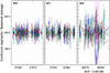 |
Fig. A.1. Example of continuum-level stability: relative fluxes in 18 pseudocontinuum segments for the Fe I 430-445 nm group, each normalized to its seasonal average. Here, as in other spectral regions, a few weeks of more noisy data appeared in 2018, and were removed from later analyses (shaded in pink). |
Even if these most significant fluctuations may appear striking on the scale of these plots, the amplitudes of even individual continuum segments remain below one percent and would go unnoticed in any more ordinary spectrophotometry. Still, since the present aim is to push photometry to its limit, data from this noisier period, June 17–28, 2018 (BJD 58,287–58,298), were excluded from all later analyses.
Except for random photometric noise, it is awkward to precisely quantify the instrumental or observational factors toward limits in photometric precision. The current analysis uses 1D data reduced from extractions from a 2D échelle spectrometer format. In principle, any ensuing resampling adds noise, but resampling cannot be avoided when we are seeking to obtain spectra with both the target lines and a sequence of pseudocontinuum references. The scatter seen in the figures throughout the paper serves to illustrate what amplitudes of microvariability that can be identified in spectra from HARPS-like instruments, although it is still challenging to ascertain what part of the finer scatter is solar and what is instrumental.
Appendix B: Spectral line selection
Fe I and Fe II line segments selected for measurements of equivalent widhts. Short- and long-wavelength limits are shown, together with the number of measured pseudocontinuum points. Wavelength values refer to those in the air.
Non-Fe line segments selected for measurements of equivalent widhts.
All Tables
Fe I and Fe II line segments selected for measurements of equivalent widhts. Short- and long-wavelength limits are shown, together with the number of measured pseudocontinuum points. Wavelength values refer to those in the air.
All Figures
|
Fig. 1. 200-yr span of sunspot numbers places current observations in a wider perspective (top). Around activity minima, days without reported sunspots are not unusual. Recent Cycle 24 with daily sunspot numbers (bottom) from WDC-SILSO (World Data Center – Sunspot Index and Long-term Solar Observations, Royal Observatory of Belgium, Brussels). Superposed red curve shows monthly averages. The selected periods from which HARPS-N data were analyzed are marked with vertical bars. |
| In the text | |
|
Fig. 2. HARPS-N observations of the Sun (top) with each exposure marked by a point (Dumusque et al. 2021). Selected exposures at the smallest airmasses (red points) occurred around daily noon during the summer seasons of 2016–2017–2018. Airmasses for the 1000 selected recordings (middle). S/N values remaining very high, but decreasing slightly over time (bottom), apparently due to diminishing telescope and instrument transmission. |
| In the text | |
|
Fig. 3. Apparent solar radial velocity (top) growing more negative with time (given as Barycentric Julian Date), apparently due to less magnetic granulation and a smaller suppression of convective blueshift. Mt.Wilson Ca II H & K S-index reflects the slowly declining activity level in the solar cycle (middle) modulated by solar rotation. Daily sunspot numbers from WDC-SILSO (bottom). The periods from which HARPS-N data were analyzed are marked in red or shaded in color. |
| In the text | |
|
Fig. 4. Example of HARPS-N spectra and selection of regions for measurement. Background thin black line: Göttingen solar flux atlas (Reiners et al. 2016). Its higher spectral resolution is evident from its deeper line profiles. Blue line: Average over 100 HARPS-N exposures. Red line: Selected regions of Fe I line absorption. Green line: Selected reference regions of quasi-continua. Thin brown line around 100%: ratio between one representative HARPS-N exposure and a 100-exposure average, illustrating the random-noise level for a single exposure with nominal S/N in grating order 50 equal to 430. The wavelength scale represents values in air (vacuum values in the Göttingen atlas were converted to those in standard air). |
| In the text | |
|
Fig. 5. Example of Fe I line selections in shortward parts of the spectrum (blue), of Fe II (green), and of Fe I at long wavelengths (dark purple). Absorption features are truncated at places of small intensity gradients, occasionally embracing several lines. Intermingled pseudocontinua, whose averages are used as an intensity reference, are marked in red. |
| In the text | |
|
Fig. 6. Relative changes of Fe I and Fe II absorption line equivalent widths during the measured periods in 2016 (red), 2017 (cyan), and 2018 (gray). Left column shows the dependence on the Mt.Wilson Ca II H & K chromospheric activity S-index; right column on the radial velocity as obtained from the full HARPS-N spectrum. A lower S/N in the grating orders housing weaker lines at the longest wavelengths accounts for a greater spread of points in the bottom frames. The lines included in each group are listed in Table B.1. |
| In the text | |
|
Fig. 7. Top: Selected portion of the Mg I 457.1 nm absorption line and its surrounding continuum reference segments (red). Center: Selection of the Mg I b line triplet lines and their continuum reference segments. Bottom: Na I D2 and D1 lines and their continuum segments. |
| In the text | |
|
Fig. 8. Relative absorption equivalent width changes in Mg I lines during the selected seasons of 2016–2017–2018 (red–cyan–gray), as function of the Mt.Wilson Ca II H & K S-index. |
| In the text | |
|
Fig. 9. Relative absorption equivalent width changes in Mg I lines during the selected observing seasons of 2016–2017–2018 (red–cyan–gray), as function of the radial velocity for the full spectrum. |
| In the text | |
|
Fig. 10. Relative changes in the absorption equivalent widths of the various Mg I lines during the selected seasons of 2016–2017–2018 (red–cyan–gray). Dotted blue lines are fits to the data. |
| In the text | |
|
Fig. 11. G-band region together with selected spectral features as observed with HARPS-N: G-band core (dotted blue), full G-band (dotted blue + green), surrounding nearby Fe I lines (black), and pseudocontinuum reference points (red). An averaged 100-exposure spectrum is plotted in thin gray. From top down, successively narrower spectral segments are shown. |
| In the text | |
|
Fig. 12. Absorption equivalent widths for the full G-band region, its central core, and nearby Fe I lines, as function of the Ca II H & K S-index. The different seasons of 2016, 2017, and 2018 are marked in red, cyan, and gray. Also, the corresponding radial velocity variations for the full spectrum are shown. For cases with apparent systematic dependences, dotted blue lines show fitted relations. |
| In the text | |
|
Fig. 13. Ratios between the full G-band fluxes and its absorption equivalent widths, the G-band core, and that of nearby Fe I lines. Different seasons of 2016, 2017, and 2018 are marked in red, cyan, and gray. Fitted relations are dotted blue lines, while the identity relations are dashed black. The core flux shows a steeper relative variability than the full band. |
| In the text | |
|
Fig. 14. Examples of selected Mn I lines with hyperfine splitting in the 540 nm region with pseudocontinuum segments marked in red. The lines are noticeably broader than others of comparable depth. The full set of sampled Mn I lines extends over the range 511–644 nm (Table B.2). |
| In the text | |
|
Fig. 15. Variations in hyperfine split Mn I lines. Data for the previously studied single line λ 539.47 nm (top row) are inconclusive but the summed equivalent widths of 16 different Mn I lines reveal a clear trend (bottom). Data for 2016–2017–2018 are shown in red–cyan–gray. |
| In the text | |
|
Fig. 16. Spectral regions around Hα, Hβ, and Hγ. Solid bold lines denote the line intervals measured; for Hβ its central core was also measured separately (dotted). In each case, lines are measured relative to local pseudocontinua marked in red, chosen symmetrically about the line centers. The average spectrum from 100 HARPS-N exposures is plotted as a thin dark line. The intensities are normalized to each local pseudocontinuum. |
| In the text | |
|
Fig. 17. Relative absorption equivalent widths for the Balmer lines Hγ, Hβ (full and core), and Hα, as function of the Mt.Wilson Ca II H & K S-index. Different colors indicate data from the observing seasons of 2016 (red), 2017 (cyan) and 2018 (gray). Because of its greater variability, the vertical scale for Hα is more extended. |
| In the text | |
|
Fig. 18. Ratios of the absorption equivalent widths for the Balmer lines Hα, the Hβ core, and Hγ, versus that of the full Hβ (Fig. 16). Red, cyan, and gray indicate data from the observing seasons of 2016, 2017, and 2018. Dashed lines show the identity ratios while those in dotted blue are fits to the data. Because of its greater variability, the horizontal scale for Hα is more extended. |
| In the text | |
|
Fig. 19. Relative variations of the measured Na I D1 and D2 absorption during the seasons of observation. Bottom: Precipitable water vapor above the Roque de los Muchachos observatory on La Palma. Time is given as Barycentric Julian Date. Spectral data from the noisier period in 2018 are omitted (Fig. A.1). |
| In the text | |
|
Fig. 20. Differential variability of absorption in Na I D1 and D2 lines. The observing seasons of 2016, 2017, and 2018 are marked in red, cyan, and gray. The identity relation is dashed while linear fits are dotted blue. The weaker Na I D1 line is more variable than the more saturated D2, while their ratio mirrors the chromospheric activity index. |
| In the text | |
|
Fig. 21. Variations in Hα flux (not absorption) measured during the 2016 data period, together with contemporaneous full-disk Hα images and (adjacent smaller circles) photospheric magnetograms, at selected labeled dates of local Hα-flux maxima or minima. Daily Hα flux averages are large red dots, individual exposures are small and black. The full-disk images were acquired by GONG instruments operated by NISP/NSO/AURA/NSF with contributions from NOAA (Global Oscillation Network Group 2024). |
| In the text | |
|
Fig. A.1. Example of continuum-level stability: relative fluxes in 18 pseudocontinuum segments for the Fe I 430-445 nm group, each normalized to its seasonal average. Here, as in other spectral regions, a few weeks of more noisy data appeared in 2018, and were removed from later analyses (shaded in pink). |
| In the text | |
Current usage metrics show cumulative count of Article Views (full-text article views including HTML views, PDF and ePub downloads, according to the available data) and Abstracts Views on Vision4Press platform.
Data correspond to usage on the plateform after 2015. The current usage metrics is available 48-96 hours after online publication and is updated daily on week days.
Initial download of the metrics may take a while.