| Issue |
A&A
Volume 676, August 2023
|
|
|---|---|---|
| Article Number | A93 | |
| Number of page(s) | 25 | |
| Section | Extragalactic astronomy | |
| DOI | https://doi.org/10.1051/0004-6361/202245718 | |
| Published online | 11 August 2023 | |
Wide-field CO isotopologue emission and the CO-to-H2 factor across the nearby spiral galaxy M101
1
Argelander-Institut für Astronomie, Universität Bonn, Auf dem Hügel 71, 53121 Bonn, Germany
e-mail: This email address is being protected from spambots. You need JavaScript enabled to view it.
2
Center for Astrophysics, Harvard & Smithsonian, 60 Garden St., 02138 Cambridge, MA, USA
3
Sterrenkundig Observatorium, Universiteit Gent, Krijgslaan 281 S9, 9000 Gent, Belgium
4
Center for Astrophysics & Space Sciences, Department of Physics, University of California San Diego, 9500 Gilman Drive, La Jolla, CA 92093, USA
5
Department of Astronomy, The Ohio State University, 140 West 18th Ave, Columbus, OH 43210, USA
6
Observatorio Astronómico Nacional (IGN), C/ Alfonso XII, 3, 28014 Madrid, Spain
7
Max Planck Institute for Astronomy, Königstuhl 17, 69117 Heidelberg, Germany
8
4-183 CCIS, University of Alberta, Edmonton, Alberta T6G 2E1, Canada
9
Institute of Astronomy and Astrophysics, Academia Sinica, No. 1, Sec. 4, Roosevelt Road, Taipei 10617, Taiwan
10
European Southern Observatory, Karl-Schwarzschild-Straße 2, 85748 Garching, Germany
11
National Astronomical Observatory of Japan, 2-21-1 Osawa, Mitaka, Tokyo 181-8588, Japan
12
Institüt für Theoretische Astrophysik, Zentrum für Astronomie der Universität Heidelberg, Albert-Ueberle-Strasse 2, 69120 Heidelberg, Germany
13
Cosmic Origins Of Life (COOL) Research DAO, coolresearch.io
14
Department of Physics & Astronomy, University of Wyoming, Laramie, WY 82071, USA
15
Sub-department of Astrophysics, Department of Physics, University of Oxford, Keble Road, Oxford OX1 3RH, UK
Received:
18
December
2022
Accepted:
1
February
2023
Abstract
Carbon monoxide (CO) emission constitutes the most widely used tracer of the bulk molecular gas in the interstellar medium (ISM) in extragalactic studies. The CO-to-H2 conversion factor, α12CO(1−0), links the observed CO emission to the total molecular gas mass. However, no single prescription perfectly describes the variation of α12CO(1−0) across all environments within and across galaxies as a function of metallicity, molecular gas opacity, line excitation, and other factors. Using spectral line observations of CO and its isotopologues mapped across a nearby galaxy, we can constrain the molecular gas conditions and link them to a variation in α12CO(1−0). Here, we present new, wide-field (10 × 10 arcmin2) IRAM 30-m telescope 1 mm and 3 mm line observations of 12CO, 13CO, and C18O across the nearby, grand-design, spiral galaxy M101. From the CO isotopologue line ratio analysis alone, we find that selective nucleosynthesis and changes in the opacity are the main drivers of the variation in the line emission across the galaxy. In a further analysis step, we estimated α12CO(1−0) using different approaches, including (i) via the dust mass surface density derived from far-IR emission as an independent tracer of the total gas surface density and (ii) local thermal equilibrium (LTE) based measurements using the optically thin 13CO(1–0) intensity. We find an average value of ⟨α12CO(1 − 0)⟩ = 4.4 ± 0.9 M⊙ pc−2 (K km s−1)−1 across the disk of the galaxy, with a decrease by a factor of 10 toward the 2 kpc central region. In contrast, we find LTE-based α12CO(1−0) values are lower by a factor of 2–3 across the disk relative to the dust-based result. Accounting for α12CO(1−0) variations, we found significantly reduced molecular gas depletion time by a factor 10 in the galaxy’s center. In conclusion, our result suggests implications for commonly derived scaling relations, such as an underestimation of the slope of the Kennicutt Schmidt law, if α12CO(1−0) variations are not accounted for.
Key words: galaxies: ISM / ISM: molecules / radio lines: galaxies
© The Authors 2023
 Open Access article, published by EDP Sciences, under the terms of the Creative Commons Attribution License (https://creativecommons.org/licenses/by/4.0), which permits unrestricted use, distribution, and reproduction in any medium, provided the original work is properly cited.
This article is published in open access under the Subscribe to Open model. This email address is being protected from spambots. You need JavaScript enabled to view it. to support open access publication.
1. Introduction
The low-J rotational transitions of carbon monoxide (CO) are key tracers of the bulk molecular gas mass in the interstellar medium (ISM) within and across galaxies. The 12CO molecule constitutes the second most abundant molecule after molecular hydrogen, H2. It has a permanent dipole moment and a much higher moment of inertia than H2. Consequently, 12CO has low energy rotational transitions, leading to excitation and detectable emission at low temperatures – unlike the lowest H2 rotational lines which require ≳100 K to excite. Hence, in particular, at low temperatures (T ∼ 10 K) and number densities above nH ∼ 102 cm−3, CO is regularly used as an effective tracer of the molecular ISM. The conversion from 12CO emission to the amount of molecular hydrogen relies on the application of an appropriate CO–to–H2 conversion factor which corresponds to a light-to-mass ratio (see the review by Bolatto et al. 2013). We note that H2 column densities, NH2 [cm−2], are generally derived from the low-J12CO(1–0) integrated intensity, W12CO(1 − 0) [K km s−1], using the conversion factor X12CO(1 − 0) [cm−2 (K km s−1)−1]:
 (1)
(1)
Equivalent to the factor XCO, but in different units, α12CO(1−0) [M⊙ pc−2 (K km s−1)−1] converts the integrated intensity into the total molecular gas mass surface density (including the contribution of elements heavier than hydrogen), Σmol [M⊙ pc−2], via:
 (2)
(2)
The value of α12CO(1−0) varies with the ISM environment. In low-metallicity regions, for example, a significant fraction of the molecular gas becomes CO-dark since dust shielding against photodissociation of CO is reduced (Maloney & Black 1988; Israel 1997; Leroy et al. 2007, 2011; Wolfire et al. 2010; Glover & Mac Low 2011; Bolatto et al. 2013; Schruba et al. 2017; Williams et al. 2019). In addition, previous studies find that α12CO(1−0) tends to decrease toward the centers of galaxies (Sandstrom et al. 2013; Cormier et al. 2018; Israel 2020). Changes in temperature and gas turbulence (e.g., Israel 2020; Sun et al. 2020; Teng et al. 2022), which both affect CO emissivity and hence the conversion factor, could explain the observed decrease in α12CO(1−0). Given that CO is so straightforwardly observable, a concrete prescription for α12CO(1−0) as a function of local ISM properties poses a longstanding goal.
Obtaining robust α12CO(1−0) calibrations is challenging since the molecular gas mass must be measured independently of CO emission. One commonly used technique consists of using dust emission to trace the combined atomic and molecular (i.e., total) gas distribution in the ISM (e.g., Thronson et al. 1988; Israel 1997; Leroy et al. 2011; Planck Collaboration XXI 2011; Sandstrom et al. 2013). From an empirical standpoint in the Milky Way, dust seems to be well mixed with the total gas at the kiloparsec-scales (Planck Collaboration XXI 2011). In addition, the dust emission remains optically thin across most nearby spiral galaxies. Using IR or (sub)millimeter emission, one can model the dust spectral energy distribution and obtain an estimate of the dust mass surface density. We can translate the dust mass to a total gas column or mass surface density using a metallicity-dependent dust-to-gas ratio (DGR). The DGR can, however, be environmentally dependent and vary across a galaxy (Roman-Duval et al. 2014). Since the ionized gas is only expected to contribute a small fraction of the column density of gas mixed with dust (Planck Collaboration XXI 2011), we can reasonably consider this dust-based column density to reflect the sum of atomic gas H I, and molecular gas. Using H I emission observations, we can separate the total gas into its two components and separate out the amount of molecular gas. By comparing it to the measured CO intensity, we can derive an estimate for α12CO(1−0).
We can also use CO isotopologue emission to infer the temperature, density, and opacity of molecular clouds in nearby galaxies (e.g., Davis 2014; Alatalo et al. 2015; Roman-Duval et al. 2016; Cormier et al. 2018; Israel 2020; Teng et al. 2022). The low-J12CO transitions usually remain optically thick, whereas 13CO and C18O are optically thinner. Consequently, comparing optically thin 13CO and C18O lines to the optically thick 12CO lines gives insights into the optical depth. Moreover, contrasting two optically thin lines offers an understanding of changes in relative abundances of the different isotopologue species (Davis 2014; Zhang et al. 2018; Brown & Wilson 2019). For instance, the various C and O isotopes and the CO isotopologue species abundances vary with processes, such as nucleosynthetic and chemical processes (Henkel et al. 1994; Timmes et al. 1995; Prantzos et al. 1996). Hence, studying the emission of several CO isotopologues can provide insight into the chemical enrichment of the molecular gas. Due to lower abundances, the emission of these CO isotopologues is, however, fainter by 1–2 orders of magnitude than the 12CO emission (e.g., den Brok et al. 2022).
Both estimating the CO-to-H2 conversion factor via the dust mass surface density and studying the molecular gas conditions using CO isotopologues require high-sensitivity observations of CO. As a result, studies that resolve these diagnostics across large parts of galaxies are still rare. Here, we present IRAM 30 m telescope observations of the J = 1 → 0 rotational transition of 12CO, 13CO, and C18O for the galaxy M101. It is a well-studied, massive, face-on, nearby (D = 6.65 Mpc; Anand et al. 2021), star-forming spiral galaxy in the northern hemisphere. In addition to its proximity, the galaxy has a low inclination (i = 18°), which allows for well-resolved, extended studies across the full galactic disk. M101 has a considerable apparent size across the sky with an extent of the disk in the optical of ∼20′×20′ (Paturel et al. 2003). It is tidally interacting (Waller et al. 1997) with nearby companion galaxies. Furthermore, M101 is of particular interest due to its well-documented metallicity gradient (Kennicutt et al. 2003; Croxall et al. 2016; Berg et al. 2020) based on auroral line measurements. The gradient is stronger than in other nearby spiral galaxies (for M101, the gradient is −1.1 dex/r25; Berg et al. 2020). In Fig. 1, we show an optical composite image using observations from the Sloan Digital Sky Survey (SSDS; Blanton et al. 2017). In addition, we show the 12CO(1–0) line map presented in this paper using overlayed contours. The galaxy has a wealth of ancillary data across all wavelength regimes. As part of the IRAM 30 m large program HERACLES (Leroy et al. 2009), wide-field 12CO(2–1) observations exist, which complement our observations of the 3 mm CO J = 1 → 0 lines. In addition, there exists a dust surface density map (Chastenet et al. 2021) and a H I map from THINGS (Walter et al. 2008) that allow resolved application of the dust-based modeling technique. Table 1 lists key properties of the galaxy derived from previous surveys and studies.
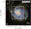 |
Fig. 1. SDSS composite RGB image with 12CO(1–0) overlay. Color image using public SDSS data from the 16th data release (Ahumada et al. 2020). We combined the u, g, and r filter bands. Contours illustrate the IRAM 30 m 12CO(1–0) integrated intensities. The mm observations have a resolution of 23″(∼800 pc), and are indicated by the black circle in the lower left. The 10′×10′ field-of-view of our IRAM 30 m observation is indicated by the white rectangular outline. Contours are drawn at arbitrary intervals between 0.5 − 10 K km s−1 to highlight the structure of the galaxy. |
Properties of M101.
The IRAM 30 m wide-field ∼kpc multi-CO line observations of M101 complement the IRAM 30 m large program CLAWS (den Brok et al. 2022), which obtained deep multi-CO kpc-scale observations of the galaxy M51. In combination, we can investigate differences and similarities in molecular gas conditions traced by CO emission between these two massive, star-forming spiral galaxies. Moreover, since we have the same suite of data for M51 as for M101, we can systematically assess the CO integrated intensity ratio (hereafter referred to as simply “CO line ratio”) and α12CO(1−0) conversion factor trends across different nearby galaxies.
This paper is organized as follows: in Sect. 2 we present and describe the IRAM 30 m observations as well as the ancillary data that are used in this paper. The main results of the paper, which includes results from the CO isotopologue analysis and the α12CO(1−0) variation across the galaxy, are presented in Sects. 3 and 4. Finally, Sect. 5 discusses the implications of the CO line ratio and α12CO(1−0) variation on commonly derived molecular ISM scaling relations and provides a parameterization of the conversion factor in terms of commonly observed parameters. We conclude in Sect. 6.
2. Observations and data reduction
2.1. Observations
As part of an IRAM 30m observing program (#160-20, PI: den Brok), we used the EMIR receivers to map line emission in the 1 mm (220 GHz) and 3 mm (100 GHz) windows in dual polarization from the disc of M101 for a total of ∼80 h (∼65 h on-source time) in the time period of January to March 2021. The receiver bandwidth was 15.6 GHz per polarization. We carried out the observations simultaneously in the E90 and E230 bands using both the upper-inner (UI) and upper-outer (UO) bands. We used the Fast Fourier Transform spectrometers with 195 kHz spectral resolution (FTS200). The spectrometer yielded a spectral resolution of ∼0.5 km s−1 for the E090 and ∼0.2 km s−1 for the E230 band. Table 2 lists the key lines we targeted.
Summary of the lines targeted as part of the IRAM 30 m observing program.
For the mapping, we used a similar approach to the one from the EMPIRE survey (see Jiménez-Donaire et al. 2019). Using the on-the-fly and position switching (OTF-PSW) mode, we mapped a field of 10 arcmin × 10 arcmin (corresponding to ∼ 20 kpc × 20 kpc or 0.83 r25 × 0.4r25). In addition, we included two emission-free reference positions (OFF position) offset by 300″ toward the north and east of M101’s center. We scanned the field in RA and Dec directions using multiple straight paths that are each offset by 8″ from each other. After an iteration over the full field, we shifted the scanned box by  , with N = 2″, 4″, 6″, along the position angle PA = +45°. This guarantees that, in the end, we cover M101 with a much finer, 2″, instead of 8″, grid along the x and y direction. We set the read-out dump time to 0.5 s, and the final spacing between data points reach 4″. A typical observation session had a length of 6 − 9 h during the night, with 11 sessions in total. The telescope’s pointing and focus were determined at the beginning of each session using observations of a bright quasar. We corrected the focus after 4 h of observing, and the pointing of the telescope was adjusted every 1 − 1.5 h using a nearby quasar. To ensure a proper antenna temperature (
 ) calibration, we did a chopper-wheel calibration every 10 − 15 min using hot-/cold-load absorber and sky measurements. Finally, to achieve accurate flux calibration, we observed line calibrators (IRC+10216 or W3OH) at the beginning or end of each observing session.
2.2. Data reduction
The following steps summarize the data processing and reduction. For these individual routines, we employ the scripts used for the HERACLES and EMPIRE pipeline (see description in Jiménez-Donaire et al. 2019) and basic calibration steps by MRTCAL1.
-
First, we convert the spectrum to the corrected antenna temperature scale (
 ) by scaling each science scan using the most recent previous calibration scan.
 -
We then subtract the most recent OFF measurement from the calibrated spectrum. This concludes the most basic calibration steps.
-
Next, using the Continuum and Line Analysis Single-dish Software (CLASS2), we extract the target lines and create the velocity axis given the rest frequency of the relevant line.
-
To subtract the baseline, we perform a constant linear fit. For the fit, we account for the systemic velocity of M101. We omit the range of 100–400 km s−1 around the center of the line (which corresponds to the velocity range of the galaxy).
-
Finally, we regrid the spectra to have a 4 km s−1 channel width across the full bandpass. Such a spectral resolution is sufficient to sample the line profile, as shown by previous observations and IRAM 30 m surveys, such as HERACLES, EMPIRE and CLAWS. The spectra are then saved as a FITS file.
To estimate the flux calibration stability, we observed the spectra of line calibrators (e.g., IRC+10216) on several nights. We find a maximum day-to-day variation in amplitude of ∼5% across all observations, which is consistent with the more extended analysis of the stability of the line calibrators in Cormier et al. (2018) done for the EMPIRE survey. The average actual noise in the cube data is listed in Table 2.
We performed a more sophisticated final data reduction using an IDL routine, which is based on the HERACLES data reduction pipeline (Leroy et al. 2009). With this routine, we can remove bad scans and problematic spectra. Furthermore, the routine performs a platforming correction at the edges of the FTS units. This ensures that the various sub-band continua are at a common level. We note that the receiver’s tuning was chosen so that no target line is affected by potential offsets due to platforming. After the platforming correction, we perform a baseline fitting again. We start by excluding a generous line window using the 12CO(1–0) line emission. We place a window extending in both spectral directions around the mean 12CO(1–0) velocity. The window’s full width for each pixel depends on the specific velocity range of the galaxy’s emission derived from HERACLES CO(2–1) data. It ranges between 50 and 300 km s−1 for each pixel. We place two windows of the same width adjacent to the central window on both sides. The pipeline then fits a second-order polynomial to the baseline in these windows. The routine finally subtracts the resulting baseline from the full spectrum.
Bad scans and spectra are removed by sorting the remaining spectra by their rms. The pipeline determines the channel-rms from line-free windows after the baseline subtraction. We remove the spectra in the highest tenth percentile.
For the following analysis, we use the main beam temperature (Tmb). The main beam temperature is connected to the corrected antenna temperature scale ( ) via
) via
 (3)
(3)
with the forward (Feff) and beam (Beff) efficiencies, which depend on the observed frequency. We determined the value of the efficiencies using a cubic interpolation of the efficiencies listed in the IRAM documentation3. Adopting these values, we find a Feff/Beff ratio of 1.2 at 115 GHz and 1.6 at 230 GHz.
Finally, we generated science-ready data cubes by gridding the spectra onto a 2″ spaced Cartesian grid. The final beam of each data cube, given in Table 2 is coarser than the telescope beam, because we performed a further convolution of the OTF data (at telescope beam resolution) with a Gaussian beam that has a width corresponding to two-thirds of the FWHM of the telescope beam. Such a gridding kernel is needed as we translate from the data sampled on the OTF grid to a regular grid (Mangum et al. 2007). Our choice of a gridding kernel equal to two-thirds of the FWHM of the telescope beam reflects a trade-off between signal-to-noise and resolution. The noise is sampled on the scale of the data dumps (every 0.5 s) while the telescope samples the sky with the PSF of the telescope. The average noise in the cube data is listed in Table 2.
This work does not account for flux contamination due to error beam contribution. We note that M101 shows no strong arm-interarm contrast in CO emission (as opposed to other similar spiral galaxies, such as, for example, M51). Therefore, the magnitude of the error beam contribution is expected to be minor. In den Brok et al. (2022), the effect of error beam contributions is discussed in detail. In particular, in the presence of strong contrast between bright and faint regions, the faint region can suffer from significant error beam contributions. The exact contribution is difficult to quantify as the exact shape of the error beam of a single-dish telescope fluctuates depending on the telescope’s elevation. That is why only first-order estimates on the extent of the contribution can be made. IRAM provides estimates of the full 30 m telescope beam pattern in their reports (e.g., Kramer et al. 2013). The 1 mm regime is more strongly affected by such error beam contributions, since the telescope’s main beam efficiency is lower ( and
and  ) and the beam size is smaller. While den Brok et al. (2022) find in general contributions to be < 10% in M51, it can in certain interarm regions reach up to 40%. In particular, regions with strong contrast are affected. For M101, we do not expect the error beam to contribute more than 10%, given the overall low contrast across its disk.
2.3. Ancillary data and measurements
For a complete analysis, we use archival and ancillary data sets. In this section, we provide a brief description of the additional data sets used in the analysis. For our α12CO(1−0) estimation approach, we particularly require robust dust mass surface density and atomic gas mass surface density maps.
2.3.1. Dust mass surface density maps
The dust surface density maps are the products of emission spectral energy distribution (SED) fitting following the procedure by Chastenet et al. (2021). They used a total of 16 photometric bands, combining mid- and far-IR maps. This includes the 3.4, 4.6, 12, 22 μm from the Wide-field Infrared Survey Explorer (WISE; Wright et al. 2010), 3.6, 4.5, 5.8, 8, 24, 70, 160 μm from Spitzer (Fazio et al. 2004; Rieke et al. 2004; Werner et al. 2004), and 70, 100, 250, 350, and 500 μm from Herschel (Griffin et al. 2010, Pilbratt et al. 2010, Poglitsch et al. 2010). For the M101 dust mass map they relied on Herschel data from KINGFISH (Kennicutt et al. 2011), Spitzer data from Dale et al. (2009), and WISE maps from the z0mgs survey (Leroy et al. 2019). The angular resolution would be ∼36″, if we include up to 500 μm. For our analysis, we employ a resolution of ∼21″ by only using up to 250 μm. The fitted dust masses up to 250 μm. is consistent with the one up to 500 μm (J. Chastenet, priv. comm.). Chastenet et al. (2021) used the Draine & Li (2007) physical dust model to fit the data, with the DustBFF fitting tool (Gordon et al. 2014). The free parameters for dust continuum emission fitting are the minimum radiation field heating the dust, Umin, the fraction of dust grains heated by a combination of radiation fields at various intensities, γ, the total dust surface density, Σdust, the fraction of grains with less than 103 carbon atoms, qPAH, and a scaling factor for stellar surface brightness, Ω*. We note that we correct the dust mass surface density with a normalization factor of 3.1 (Chastenet et al. 2021). The renormalization is necessary so that the dust mass estimates agree with predictions based on the metal content (e.g., Planck Collaboration Int. XVII 2014; Planck Collaboration Int. XXII 2015; Dalcanton et al. 2015). Chastenet et al. (2021) derived the value 3.1 by fitting the dust model to a common MW diffuse emission spectrum and comparing to other dust models using the same abundance constraints. The uncertainty is set pixelwise as 10% of the dust mass surface density value. Details on IR image preparation, fitting procedure, and results can be found in Chastenet et al. (2021).
2.3.2. Radial metallicity gradients
We employ radial metallicity gradient measurements from Berg et al. (2020). They derive the chemical abundances from optical auroral line measurements in H II regions across M101 and M51. Their observations are part of the CHemical Abundances Of Spirals (CHAOS) project (Berg et al. 2015). We use the slope and intercept of the gradient provided by Berg et al. (2020; see Table 2 therein, we correct the slope since we use an updated value for M101’s r25):
![Mathematical equation: $$ \begin{aligned} 12+\log (\mathrm O/H)={\left\{ \begin{array}{ll}(8.78{\pm }0.04)-(1.10{\pm }0.07)R_{g}[r_{25}]&\text{ for} \text{ M101} \\ (8.75{\pm }0.09)-(0.27{\pm }0.15)R_{g}[r_{25}]&\text{ for} \text{ M51}\end{array}\right.}. \end{aligned} $$](/articles/aa/full_html/2023/08/aa45718-22/aa45718-22-eq10.gif) (4)
(4)
Often, the metallicity is also expressed in terms of solar metallicity fraction, Z. We assume a solar abundance of 12 + log10(O/H)⊙ = 8.73 (Lodders 2010) and convert the oxygen abundance to a metallicity (Z = Σmetal/Σgas, where Σgas includes the mass of He as well). The following equation relates the fractional metallicity, Z, to the oxygen abundance:
 (5)
(5)
We assume a fixed oxygen-to-metals ratio, MO/Mmetal = 0.51 (Lodders 2003). The atomic masses for oxygen and hydrogen are indicated by mO and mH, respectively. The factor 1.36 is used to include Helium.
2.3.3. Atomic gas surface density
To estimate the atomic gas surface density (Σatom), we use archival H I 21 cm line emission data from The H I Nearby Galaxy Survey (THINGS; Walter et al. 2008). The data were observed with the Very Large Array (VLA) in B, C, and D configurations. We use the natural weighted data. These have an angular resolution of ∼11″(∼350 pc) and a spectral resolution of ∼5 km s−1. We note that the THINGS M101 data suffer from a negative baseline level due to missing zero-spacings. To improve the data, we feathered the interferometric VLA data using an Effelsberg single dish observation from The Effelsberg-Bonn H I Survey (EBHIS; Winkel et al. 2016). We use uvcombine4 and the CASA version 5.6.1 feather function and determine a single dish factor of 1.7. We convert the H I line emission (IH I) to atomic gas surface density via (Walter et al. 2008):
![Mathematical equation: $$ \begin{aligned} \Sigma _{\mathrm{H}\,i } [M_\odot \,\mathrm{pc}^{-2}] = 1.36\times (8.86\times 10^3)\times \left(\frac{I_{\mathrm{H}\,i } [\mathrm{Jy\,beam^{-1}\,km\,s^{-1}}]}{{B_{\rm maj}[^{\prime \prime }]\times B_{\rm min}[^{\prime \prime }]}}\right), \end{aligned} $$](/articles/aa/full_html/2023/08/aa45718-22/aa45718-22-eq12.gif) (6)
(6)
where the factor 1.36 accounts for the mass of helium and heavy elements and assumes optically thin 21-cm emission. Bmax and Bmin are the FWHM of the major and minor axes of the main beam mentioned above. We provide further details on the feathering and how it affects the subsequent H I measurements in Appendix A.
2.3.4. Stellar mass and SFR data
We employ stellar mass and SFR surface density maps from the z0mgs survey (Leroy et al. 2019). The SFR surface density is estimated using a combination of ultraviolet observations from the Galaxy Evolution Explorer (GALEX; Martin et al. 2005) and mid-infrared data from the Wide-field Infrared Survey Explorer (WISE; Wright et al. 2010). We use the SFR maps with the combination FUV (from GALEX; at 150 nm wavelength) + WISE4 (from WISE; at 22 μm).
We use the stellar mass surface density maps computed with the technique utilized for sources in the PHANGS-ALMA survey (Leroy et al. 2021). In short, the Σ⋆ estimate is based on near-infrared emission observations at 3.6 μm (IRAC1 on Spitzer) or 3.4 μm (WISE1). The final stellar mass is then derived from the NIR emission using an SFR-dependent mass-to-light ratio.
2.4. Final data product
For the analysis in this paper, we homogenize the resolution of the data. We convolve all observations to a common angular resolution of 27″(= 840 pc), adopting a Gaussian 2D kernel. We regrid all data onto a hexagonal grid where the points are separated by half the beam size (13″). We perform these steps using a modified pipeline, which has been utilized for IRAM 30 m large programs before (EMPIRE, Jiménez-Donaire et al. 2019; CLAWS, den Brok et al. 2022).
We use the HERACLES/EMPIRE pipeline to determine the integrated intensity for the individual pixels in the regridded cube for each line, including H I. The goal is to create a signal mask that helps optimize the S/N of the derived integrated intensities. The masked region over which to integrate is determined using a bright emission line. Since H I is faint in the center, we use the 12CO(1–0) line for the mask determination for pixels with a galactocentric radius r ≤ 0.23 × r25. We select the factor 0.23, because, based on observations of star-forming galaxies, the CO surface brightness drops, on average, by a factor of 1/e at this radius (Puschnig et al. 2020). This ensures that 12CO is still detected significantly relative to the H I emission line. For lines of sight with a larger galactocentric radius, the routine employs the H I emission line to determine the relevant spectral range. We make a 3D mask where emission is detected at S/N > 4 and then expand the resulting mask into regions with S/N > 2 detections. Finally, we pad the mask along the spectral axis by ±2 channels in velocity. The integrated intensity is then computed by integrating over the channels within the mask. Indicating the number of channels within the mask by nchan, the routine computes as follows:
![Mathematical equation: $$ \begin{aligned} W_{\rm line}[\mathrm{K}\,\mathrm{km}\,\mathrm{s}^{-1}] = \sum ^{n_{\rm chan}} T_\mathrm{mb} (v)[\mathrm{K}] \cdot \Delta v_{\rm chan}[\mathrm{km}\,\mathrm{s}^{-1}] \end{aligned} $$](/articles/aa/full_html/2023/08/aa45718-22/aa45718-22-eq13.gif) (7)
(7)
where Tmb is the surface brightness temperature of a given channel and Δvchan is the channel width. Figure 2 shows the integrated intensity for the 12CO(1–0), 12CO(2–1), and 13CO(1–0) emission lines. The uncertainty of the integrated intensity for each sightline is computed using the final convolved and regridded cubes with the following equation:
![Mathematical equation: $$ \begin{aligned} \sigma _W[\mathrm{K}\,\mathrm{km}\,\mathrm{s}^{-1}] = \sqrt{n_{\rm chan}}\cdot \sigma _{\rm rms}[\mathrm{K}] \cdot \Delta v_{\rm chan}[\mathrm{km}\,\mathrm{s}^{-1}]. \end{aligned} $$](/articles/aa/full_html/2023/08/aa45718-22/aa45718-22-eq14.gif) (8)
(8)
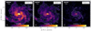 |
Fig. 2. Integrated intensities. All maps have been convolved to a common beamsize of 27″ (the beamsize is indicated by the circle in the lower left corner). Color scale in units K km s−1. Contour indicates S/N = 5 of the respective CO isotopologue transition. We do not provide the C18O(1–0) emission line map since we do not detect significant emission across the galaxy. Coordinates are relative to the center coordinates in Table 1. |
We indicate the position-dependent 1σ root-mean-squared (rms) value of the noise per channel with σrms. Our approach does not assume any variation of the noise with frequency for each target line. To determine the channel noise, the routine computes the median absolute deviation across the signal-free part of the spectrum scaled by a factor of 1.4826 (to convert to a standard deviation equivalent).
3. Results: CO isotopologue line emission
3.1. CO emission across M101
In Fig. 2, we show the moment-0 maps of 12CO(1–0) and (2–1), and 13CO(1–0). We detect significant 12CO(1–0) and (2–1) integrated intensities across the full 10′×10′ field-of-view. We see elevated emission tracing the galaxy’s bar and spiral arms. We also find higher integrated intensity values relative to the surroundings at the eastern tip of the southern spiral arm. We find significant 13CO(1–0) integrated intensities within rgal ≲ 5 kpc. The C18O(1–0) is too faint, and we do not detect any integrated intensity at S/N > 3.
To improve the S/N, we stack the spectra by binning sightlines according to various parameters. The procedure is described in Appendix C. For a full reference, Fig. C.1 shows the radially stacked spectra of the 12CO(1–0) and 13CO(1–0) integrated intensity. We stack the spectra in radial bins with a step size of 1.25 kpc out to 10 kpc. Thanks to the improved S/N in the stacked spectra, we do find significant (S/N > 3) 13CO(1–0) integrated intensity out to rgal ≤ 8 kpc. However, C18O(1–0) emission remains undetected for our 1.25 kpc radial bins and even when stacking all central 4 kpc sightlines (Fig. 3). In Fig. 3, we show for comparison the expected range of integrated intensities based on the 13CO(1–0) integrated intensity and the assumption of a C18O/13CO(1–0) ≡ R18/13 line ratio commonly found in spiral galaxies of 0.2 > R18/13 > 0.1 (Langer & Penzias 1993; Jiménez-Donaire et al. 2017). The integrated intensity is lower by a factor ∼2 from the predicted range (we find a 3σ upper limit Wul = 0.1 K km s−1 and predicted based ratio derived in nearby galaxies Wpred. = 0.15 − 0.2 K km s−1 with an average uncertainty of 0.01 K km s−1). For comparison, ratios commonly found in the literature range from R18/13 > 1 in ULIRGs (Brown & Wilson 2019), to R18/13 ∼ 0.3 in starburst (Tan et al. 2011), R18/13 ∼ 0.1 in the Milky Way (Langer & Penzias 1993), and R18/13 ∼ 0.15 for nearby spiral galaxies (EMPIRE; Jiménez-Donaire et al. 2017).
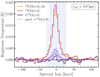 |
Fig. 3. Radially stacked CO spectra for rgal ≤ 4 kpc. We stack over the central 4 kpc. Furthermore, the predicted C18O(1–0) emission line is shown, based on the 13CO(1–0) emission line and assuming a line ratio of 0.2 > R18/13 > 0.1 (Jiménez-Donaire et al. 2017). The C18O(1–0) in M101 seems to be fainter than we would expect based on values from EMPIRE. The blue-shaded background indicates the line mask over which we integrate the spectrum. |
3.2. CO line ratios
We reiterate that we refer to the integrated intensity ratio between two lines simply as line ratio. We investigate the line ratio distribution across M101 and compare it to literature values from previous studies. The 12CO(1–0) and (2–1), as well as the 13CO(1–0) emission, is bright enough so that we can investigate its variation across the field-of-view. In particular, the following line ratios are of interest:
 (9)
(9)
 (10)
(10)
 (11)
(11)
In Fig. 4, we compare the average line ratio value R21 and R13/12 which we determined across the full field-of-view (see Table 3) with values measured in the literature. We illustrate the spatial variation of these two line ratios and their radial trends in Fig. 5. We show the line ratio of the individual sightlines as well as the radially stacked ones discussed in Sect. 3.1, which have a radial bin size of 1.25 kpc. Furthermore, we illustrate the censored region in the line ratio parameter space (see Fig. 5). This indicates the region in the parameter space where at least one of the lines is not detected with more than 1σ significance (see Appendix B for a description of the censored region). In addition, we compare the line ratio to ΣSFR, which traces changes in temperature and density of the gas (Narayanan et al. 2012). We note that previous studies found a trend of R21 with the SFR surface density, which would make it a potential tracer of line ratio variation (e.g., Sawada et al. 2001; Yajima et al. 2021; Leroy et al. 2022).
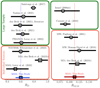 |
Fig. 4. CO line ratio comparison to literature values. We compare the average R21 and R13/12 values estimated from the distribution of the M101 data points to literature values. Errorbars indicate the 1σ distribution of sample values. If the literature value corresponds to the value for a specific galaxy, the source’s name is provided. Measurement for M101 indicated by the cross. The square symbol indicates the result from M51. Left: collection of R21 distributions. Right: the R13/12 distribution is shown. Our measurement agrees well with results for M51 and the Milky Way. |
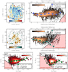 |
Fig. 5. Spatial and radial variation of the CO line ratio. Top row shows the R21 line ratio while the central row shows the R13/12 line ratio. The maps (left top and middle panels) show the spatial distribution of the line ratios. The colored points show sightlines with 5σ in both integrated intensities. The 5σ contour of the 12CO(1–0) integrated intensity is shown by the solid contour. The dashed circles indicate the radial bins used for the stacking. The radial plots (right panels) show the radial trends of the line ratios. The panels in the bottom row show trends of the 12CO(2–1)/(1–0) (R21) ratio (left) and the 13CO/12CO(1–0) ratio (R13/12) (right) with the SFR surface density. The ratio derived by the stacked line brightness is indicated by the larger blue or green symbols (see Appendix C for a brief description of the stacking technique). We note that because the S/N13CO(1–0) is significantly lower than for 12CO(1–0), and more lines of sights do not show a significant detection, the stacked points yield a lower R13/12. Triangles indicate 3σ upper limits. The uncertainty of the points is indicated, but it is generally smaller than the point size. The censored region applying to the individual lines of sight is shown by the red (1σ) shaded region. The region indicates where, due to the lower average sensitivity of one observation set, we do not expect to find significantly detected data points (i.e., the region where only one dataset will be significantly detected). |
Mean values and Kendall’s τ rank correlation coefficient (p-value given in parenthesis).
3.2.1. R21 line ratio
We compare the intensity-weighted mean R21 value in Fig. 4 to the line ratio distribution within and across other sources and samples. Regarding individual sources (orange box in Fig. 4), our result agrees well to within 1σ with the ratio of 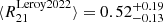 reported for this galaxy by (Leroy et al. 2022), based on IRAM 30 m HERA and NRO data. There is only a mild increase of the ratio within the central region (rgal < 1 kpc), with a line ratio of 0.69 for the central sightline. Also, the center of NGC 6946 shows a similar dynamical range of
 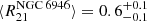 (Eibensteiner et al. 2022). M51 with ratio
 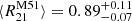 remains an outlier to all these studies as already noted by den Brok et al. (2022). Additionally, we compare it to the overall ratio distribution within a sample of galaxies (green box in Fig. 4). When contrasting our average result of M101 to the full EMPIRE survey, which consists of nine nearby spiral galaxies, we find an almost identical median value: den Brok et al. (2021) report
 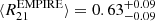 . In addition, our value agrees well with the average line ratio for a set of literature single-pointing measurements of nearby spiral galaxies, namely
  , which den Brok et al. (2021) have compiled. Yajima et al. (2021) find an average
  , which agrees with our finding in M101 within the error margins. Recently, Leroy et al. (2022) investigated R21 on kpc-scales for a large sample of CO maps of nearby galaxies. They report a median line ratio across all galaxies studied of
  . Finally, we find that the average value derived from xCOLD GASS measurements (Saintonge et al. 2017) is slightly higher with
  than the value we find. We note that the xCOLD GASS includes galaxies with high star formation rates, which could be associated with enhanced R21. Overall, we see that our average value found in M101 agrees well with those derived from a larger set of nearby star-forming spiral galaxies.
Regarding internal variation of the R21 line ratio across M101, we find no radial trend for the individual lines of sight as well as the stacked values (see the top right panel in Fig. 5). Also, Kendall’s τ correlation coefficient does not indicate any significant correlation (see Table 3). We do not find any significant azimuthal variation of R21 across the galaxy. This is qualitatively seen in the map in the top left panel of Fig. 5. Neither the bar ends nor the spiral arm or interarm regions show a significant difference in the line ratio. Also, when we bin by spiral phase, a method to quantify the difference between arm and interarm regions, we do not see any clear trend (see Appendix C). Across the full galaxy, we find a 12CO(1–0) brightness weighted mean ratio of  . Comparing to the nine galaxies of the EMPIRE sample, den Brok et al. (2021) generally find a significant increase of R21 toward the center by 10–20% in the galaxies that have a barred structure. In contrast, M101 does not seem to conform to this trend. The fact that the line ratio stays constant across the galaxy, despite apparent environmental differences in the molecular gas condition (such as center or disk, arm or interarm), puts constraints on the connection of R21 to the environmental temperature and density variation.
Past studies describe a way to parametrize R21 variation using the SFR surface density, ΣSFR (den Brok et al. 2021; Leroy et al. 2022). Understanding ways to parameterize R21 is particularly crucial for studies that rely on 12CO(2–1) as opposed to 12CO(1–0) observations to derive molecular gas parameters and hence need an accurately calibrated R21 to predict the 12CO(1–0) brightness from other J lines. The bottom row of Fig. 5 shows the distribution of the line ratios for the individual sightlines with the SFR surface density. We also show the stacked line ratio to better illustrate the trends. When looking at the stacked points, we find a significant (p = 4 × 10⁻⁴) positive (τ = 0.92) correlation for R21 with the SFR surface density, ΣSFR. A positive correlation with SFR surface density is also reported by Leroy et al. (2022) who, studying the PHANGS-ALMA sample, found a Spearman’s rank correlation coefficient of ρ = 0.55 for the galaxy-wide, normalized binned R21 to the normalized SFR surface density. Comparing the slope of the correlation in logarithmic space, we find a slightly shallower slope of m = 0.10 ± 0.2, compared to m = 0.13 found by Leroy et al. (2022). So despite the overall flat R21 trend across M101, we can still recover the trend with ΣSFR for the stacked data points, which is in agreement with previous studies. Regarding the individual lines of sight, the scatter of > 0.2 dex still dominates over the degree of variation of R21 expected from the dynamical range in ΣSFR of 2 dex.
3.2.2. R13/12 line ratio
We compare the intensity weighted mean R13/12 line ratio distribution of M101 to findings of various previous studies in Fig. 4 (right panel). The average ratio of  found in M51 (den Brok et al. 2022) is consistent within the error margin with the average ratio we find in this study, however, its scatter is slightly larger. Cormier et al. (2018) studied the 12CO-to-13CO line ratio (i.e., the inverse of the ratio we investigate) for the nine EMPIRE galaxies. Converting their finding to R13/12, they obtain
  , again consistent with our finding. Similarly, studying the central ∼20″ of around ten nearby galaxies, including AGN and central starbursts, a range of 0.06 < R13/12 < 0.13 is found by Israel (2009a,b). For comparison, we also show measurements from the Milky Way (Paglione et al. 2001). For galactic radii larger than 2 kpc, they find an average value of
  .
.
Regarding resolved line ratios within a galaxy, we find for R13/12 a negative radial trend when looking at the stacked data points (shown in the bottom right panel in Fig. 5) with a Kendall’s coefficient of τ = −0.90 and a p-value of p = 0.003 (we consider a correlation with a p-value below 0.05 to be significant). We note that using the stacked data points, we can actually sample the censored region, which applies to the individual lines of sight, as we have significant 13CO(1–0) integrated intensities out to ∼8 kpc (see Sect. 3.1 and Fig. C.1). The trend is less evident when looking at individual sightlines, as the scatter seems significantly larger than the radial trend, and we are limited by the censored region. We find an average line ratio of  . The stacked integrated intensities decreases from R13/12|rgal = 0 = 0.113 ± 0.004 down to R13/12|rgal = 8 kpc = 0.055 ± 0.005 further out. Such a radial decrease is also present in M51 (den Brok et al. 2022). For comparison, studying this ratio in the Milky Way, Roman-Duval et al. (2016) find a radial gradient of the ratio decreasing from R13/12 = 0.16 at 4 kpc to R13/12 = 0.1 at 8 kpc radial distance. This Milky Way finding agrees well with our finding in M101. The map at the middle left in Fig. 5 does also not show any azimuthal variation of the line ratio. However, we note that the significant sightlines are mainly from the center, bar ends, and spiral arm regions, while the 13CO(1–0) emission within the interarm regions is too faint. The variation of this particular line ratio is due to a combined effect of variation of the optical depth of 12CO line emission and differences in the relative abundance of 13CO and 12CO (under the assumption that 13CO remains optically thin on kpc scales; see Sect. 5.1).
Finally, we investigate the distribution of the CO line ratio across the disk of the galaxy with respect to the SFR surface density (see bottom right panel of Fig. 5). The stacked R13/12 data points show only a mild positive trend (τ = 0.73) with the SFR surface density (p = 0.06), with a scatter of ∼0.25 dex for the individual sightlines. However, we note that M101 shows only a narrow dynamical range of SFR surface densities. For comparison, M51 covers > 2 dex in SFR surface densities, while M101 shows approximately 1 dex. We note that a similar mild positive trend is observed within individual nearby galaxies (Cao et al. 2017; Cormier et al. 2018) with respect to the SFR surface density.
4. Results: CO-to-H2 conversion factor
4.1. α12CO(1 − 0) estimation
Under the assumption that dust and gas are well mixed on the scales we probe, the following relation connects the dust mass and the total gas surface density (both in units of M⊙ pc−2) via the dust-to-gas ratio (DGR):
 (12)
(12)
where α12CO(1−0) is the CO-to-H2 conversion factor in units of [M⊙ pc−2 (K km s−1)−1], which converts the CO-integrated intensity into a molecular gas mass surface density. There are, however, two unknown quantities in Eq. (12): The key parameter of interest, α12CO(1−0) and the DGR value. Both parameters are expected to vary with the galactic environment and are likely also linked to each other. To estimate both parameters, we introduce some modifications to the so-called scatter minimization technique developed in Leroy et al. (2011) and Sandstrom et al. (2013). The idea is to solve simultaneously for α12CO(1−0) and DGR. In essence, we find and select a value for α12CO(1−0) which – given a set of measurements of ΣH I, Σdust and  – yields the most uniform distribution of DGR values over a certain (∼3 kpc size) area. The approach consists of the following steps:
-
We split the galaxy into so-called solution pixels, which are hexagonal regions containing 37 half-beam sampled data points. The solution pixels are separated center-to-center by 1.5 times the beam size (panel (i) in Fig. 6 illustrates a solution pixel in red).
-
Using Eq. (12), we compute the DGR for each solution pixel with the underlying pixel using a range of α12CO(1−0) values. For α12CO(1−0) we vary the value from 0.01 to 10 M⊙ pc (K km s−1)−1 in steps of 0.1 dex (panel (iii) in Fig. 6 shows the resulting DGR values using three different α12CO(1−0) values A, B, and C). The scatter in the resulting DGR values for each solution pixel will vary with the choice of α12CO(1−0).
-
In addition to obtaining 37 DGR data points per solution pixel from 12CO(1–0), we obtain an additional 37 measurements by using the 12CO(2–1) integrated intensity measurements. We convert these to a 12CO(1–0) integrated intensity using the average R21 of the solution pixel.
-
The α12CO(1−0) value of the solution pixel is chosen such that the scatter of the DGR values of the combined 74 data points is minimal.
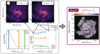 |
Fig. 6. Solution pixel approach to estimate α12CO(1−0). Left: from the scatter minimization approach, described by Leroy et al. (2011) and Sandstrom et al. (2013), we obtain estimates of α12CO(1−0) and DGR. The top panels (i) show the hexagons that illustrate the individual solution pixels for both 12CO(1–0) and (2–1) transmission. The solution pixels consist of 37 underlying, half-beam spaced lines of sight. We note that the underlying hexagon tiling is meant to show the results in each solution pixel (the actual solution pixels have 40% overlap). In the maps, we highlight an individual solution pixel. We vary α12CO(1−0) and compute the DGR following Eq. (12). We select the value for which the variation in DGR is minimal. The bottom left panel (ii) shows the variation of the DGR as a function of different α12CO(1−0). The variation for the selected solution pixel is minimal for α12CO(1−0) labeled B. We perform this analysis for each solution pixel. The bottom right panel (iii) illustrates why the variance differs when changing α12CO(1−0). Here we combine all significant points from the solution pixel indicated in panel (i) from both CO lines. The black lines point to the solution pixel where the individual lines of sight are drawn from. We correct the 12CO(2–1) data with the average line ratio of the solution pixel. The panel illustrates the differences in DGR for three selected α12CO(1−0) (labeled A, B, and C). Based on the selection of α12CO(1−0) the DGR values will be positively or negatively correlated (as illustrated by the colored line, which is drawn schematically to guide the eye). Right: the resulting α12CO(1−0) value for each solution pixel based on the combined 12CO(1–0) and 12CO(2–1) integrated intensities. |
For a more detailed description of the implementation, we refer to Sect. 3 in Sandstrom et al. (2013). We note that the solution pixels overlap (they share ∼40% of the area with the neighboring solution pixels). Consequently, they are not fully independent from each other. We illustrate the solution pixel in Fig. 6 (the pixel colored in red illustrates the full extent of a solution pixel).
With this approach, we have now constraints on the values of α12CO(1−0) and DGR. The approach makes the following assumptions:
-
There is a dynamical range in the
 ratio (x axis of the panel (iii) in Fig. 6) beyond statistical scatter. Otherwise, there is no leverage by varying α12CO(1−0) to find the minimum variation in the DGR values. We test for any potential degeneracies of the scatter minimization solution in Appendix F in case the dynamical range is limited.
 -
Regarding the DGR value: we assume that the total gas and dust are well mixed on ∼kpc scales. This ensures that Eq. (12) is valid. Furthermore, we assume that DGR remains constant on ∼3 kpc scales, DGR does not change with varying atomic and molecular phase balance, and a negligible fraction of dust is present in the ionized gas phase.
-
[Inline398
] remains constant over the scales of a solution pixel. This is justified given the generally flat line ratio trends found across other nearby galaxies, with only mild increases of 10% toward some galaxy centers (den Brok et al. 2021).
We estimate the uncertainty of the α12CO(1−0) value by performing a Monte Carlo test. For each measurement (ΣH I, Σdust and  ) we add random noise drawn from a normal distribution with the width corresponding to their measurement errors. We repeat this resampling 100 times. Our final α12CO(1−0) value and corresponding uncertainty are determined via bootstrapping. Iterating with niter = 1000, we draw nsample = 1000 samples from the Monte Carlo iterations and take the mean and standard deviation.
We note as a caveat that we do not account for systematic uncertainties in dust mass measurements. Phase-dependent depletion is observed, and the DGR is likely higher in dense, molecular regions (Jenkins 2009). On the other hand, the dust appears to emit more effectively in dense regions (Dwek 1998; Paradis et al. 2009; Köhler et al. 2015). These effects are discussed in detail in Leroy et al. (2011), Sandstrom et al. (2013). They find that variation in DGR and dust emissivity could lead to a bias of α12CO(1−0) towards higher values (by a factor of < 2). Further systematic uncertainties could be introduced by the variation of the dust-to-metals ratio, the emissivity calibration, or dust absorption coefficient (e.g., Clark et al. 2016, 2019; Chiang et al. 2018; Chastenet et al. 2021). We note that such a trend is systematic and cannot explain any galaxy-internal variation (such as a radial trend) we find in M101. Overall, such effects could be considered by updates to the scatter minimization technique in future work. We also do not account for changes in the conversion factor due to CO freeze-out, which occurs predominantly in the densest regions of molecular clouds ( ; e.g., Whitworth & Jaffa 2018). Since the low-J CO emission is optically thick, we do not expect a significant impact on the observed CO integrated intensity (hence leading to a change in the conversion factor). This is further supported by simulations from Glover & Clark (2016), who find that in molecular clouds at solar neighborhood metallicity CO freeze-out affects the derived CO-to-H2 conversion factor by only 2 − 3%.
4.2. Trends in α12CO(1−0) distribution
The panel on the right-hand side in Fig. 6 shows the spatial distribution of the estimated α12CO(1−0). From a qualitative assessment, we find a decrease in α12CO(1−0) and an increase of the DGR toward the center of the galaxy. Fig. 7 shows the radial trend of α12CO(1−0)as well as the residual. The result illustrates the lower α12CO(1−0) values towards the center, while it has a relatively constant value inside the disk (r > 2 kpc). For the central solution pixel, we have α12CO(1−0)center = (0.43 ± 0.03) M⊙ pc−2 (K km s−1)−1, while the average value in the disk amounts to ⟨α12CO(1 − 0)⟩|disk = (4.4 ± 0.9) M⊙ pc−2 (K km s−1)−1. However, we find a large 1σ point-to-point scatter in α12CO(1−0) inside the disk of ∼0.3 dex. Based on our Monte Carlo implementation of iteratively computing α12CO(1−0), we find that the propagated uncertainty of α12CO(1−0) is ∼0.1 dex. Table 4 lists the α12CO(1−0) values using different binnings.
 |
Fig. 7. Radial α12CO(1−0) and DGR trend in M101. The left panel shows radial α12CO(1−0) trend, and the right panel illustrates radial DGR dependency. Top: smaller blue (pink) points show the individual α12CO(1−0) (DGR) measurements for the various solution pixels. Larger red (yellow) points show the derived trend based on binning the data. Bottom: residual α12CO(1−0) or DGR values after subtracting the radial trend based on linearly interpolating the binned data trend (solid red /yellow line). |
Median α12CO(1−0) values for M101 and M51.
Our finding of low α12CO(1−0) values toward the center is consistent with other studies targeting larger samples of galaxies. They find conversion factors 5 − 10 times lower than the average MW factor in the center of nearby spiral galaxies (Israel 1997, 2020; Sandstrom et al. 2013). For reference, past studies also found such low values, for example, for LIRGs (e.g., Downes & Solomon 1998; Kamenetzky et al. 2014; Sliwa et al. 2017), likely due to more excited or turbulent gas similar to conditions in galaxy centers. We also note that, in particular, the low conversion factor value we find for the center of M101 is consistent with the optically thin 12CO emission limit. In the presence of highly turbulent gas motions or large gas velocity dispersion, it is possible that the low-J12CO emission turns less optically thick. In fact, the R13/12 line ratio gives us a potential way to assess whether 12CO becomes optically thin toward the center. The middle right panel in Fig. 5 shows a decreasing radial trend of R13/12. If the trend is only due to optical depth changes of 12CO, we would expect an opposite trend with decreasing R12/13 toward the center. Hence, if the 12CO emission is indeed less optically thick in the center, the observed trend in R12/13 implies that the relative abundance of 13CO has to increase toward the center of M101, and we can make a prediction of α12CO(1−0). Under representative molecular ISM conditions with an excitation temperature of Tex = 30 K, a canonical CO abundance of [CO/H2] = 10−4, and assuming local thermal equilibrium (LTE), we expect  (Bolatto et al. 2013), which is very close to the value we find for the center of M101.
We note that M101 is also included in the sample investigated by Sandstrom et al. (2013). They find a central α12CO(1−0)value of  , which lies within the margin of error of the value we find (α12CO(1 − 0)center = 0.43 ± 0.05). However, they find a galaxy-wide average value of ⟨α12CO(1 − 0)S13⟩ = 2.3, which is a factor 2 lower than the value we find in this study. To test the impact of different datasets, we repeat the α12CO(1−0) estimation using a different combination of 12CO(2–1) (CLAWS and HERACLES) and H I (non-feathered and feathered) datasets. This way, we can assess how the difference in datasets affects the resulting α12CO(1−0) values. For details on the comparison, we refer to Appendix E. The discrepancy between the median α12CO(1−0) value measured here and that from Sandstrom et al. (2013) can be traced back to the fact that Sandstrom et al. (2013) relied on 12CO(2–1) observations from IRAM 30 m/HERA, used a constant R21 = 0.7 ratio to convert between the J = 2 → 1 and J = 1 → 0 transition and used THINGS H I data that have not been short-spacing corrected. On the one hand, we find from our analysis that substituting the CLAWS data with the HERACLES 12CO(2–1) observations does not significantly affect the average α12CO(1−0) distribution. On the other hand, using the non-feathered H I data lowers the α12CO(1−0) measurements by 0.1 dex. We also find that using a constant R21 and only relying on the 12CO(2–1) observations, will further systematically lower α12CO(1−0) by 0.2 dex, hence reproducing the results from Sandstrom et al. (2013).
Contrasting our finding to results from studies using another α12CO(1−0) estimation approach, we find that our median α12CO(1−0) value for the disk of M101 is, in fact, consistent with virial mass measurements. For example, Rebolledo et al. (2015) studied the conversion factor in certain brighter regions of M101 and found, on average, values close to the MW average.
4.3. α12CO(1 − 0) based on multi-line modeling
Using the 13CO(1–0) emission line, we can perform a simple LTE modeling attempt to obtain an additional, independent estimate of α12CO(1−0), which we refer to hereafter as α12CO(1 − 0)LTE. Assuming LTE, we can calculate the conversion factor using the following equation
![Mathematical equation: $$ \begin{aligned} \alpha _{^{12}\mathrm{CO}(1{-}0)}^\mathrm{LTE} = \left[\frac{\mathrm{H}_2}{\mathrm{^{13}CO}}\right]\times \frac{\eta _{\rm 12}}{\eta _{\rm 13}}\times \frac{6.5\times 10^{-6}}{1-\exp (-5.29/T_{\rm exc})}\times R_{13/12}. \end{aligned} $$](/articles/aa/full_html/2023/08/aa45718-22/aa45718-22-eq54.gif) (13)
(13)
In this formula, the CO isotopologue line ratio R13/12 traces the optical depth, Texc indicates the excitation temperature of 13CO, ![Mathematical equation: $ \left[\frac{\mathrm{H}_2}{\mathrm{^{13}CO}}\right] $](/articles/aa/full_html/2023/08/aa45718-22/aa45718-22-eq55.gif) describes the relative 13CO abundance, and η is the beam filling factor of the 12CO(1–0) and 13CO(1–0) emission respectively. We refer to Jiménez-Donaire et al. (2017) for a more detailed derivation of the equation.
describes the relative 13CO abundance, and η is the beam filling factor of the 12CO(1–0) and 13CO(1–0) emission respectively. We refer to Jiménez-Donaire et al. (2017) for a more detailed derivation of the equation.
Figure 8 shows the derived α12CO(1 − 0)LTE values as a function of the galactocentric radius. We use two different approaches to estimate the input parameters (besides R13/12) in Eq. (13):
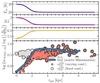 |
Fig. 8. 13CO derived α12CO(1 − 0)LTE We estimate the conversion factor under LTE assumptions using the 12CO(1–0) and 13CO(1–0) emission. We perform two iterations: (i) keeping the conditions fixed across the galaxy apart from the R13/12 ratio and (ii) varying the 13CO excitation temperature,Tex, the beam filling factor ratio, η12/η13, and the 13CO abundance between disk and center using a sigmoid function. Top three panels: variation of input parameters for α12CO(1−0) derivation. Bottom Panel: radial Trend in |


(i) We assume constant LTE conditions so that the lines are thermalized across M101 following values provided in Cormier et al. (2018). In particular, we fix the excitation temperature Tex = 20 K, the beam filling factor ratio η12/η13 = 1, and the 13CO abundance ![Mathematical equation: $ [\rm H_2/{^{13}\mathrm{CO}}]=1\times10^{6} $](/articles/aa/full_html/2023/08/aa45718-22/aa45718-22-eq58.gif) . These values are adopted from Cormier et al. (2018). The result is indicated by the grey points in Fig. 8. We find a relatively flat trend with
. These values are adopted from Cormier et al. (2018). The result is indicated by the grey points in Fig. 8. We find a relatively flat trend with  .
.
(ii) Because the molecular gas conditions are likely not constant across the galaxy, we perform the α12CO(1 − 0)LTE calculation again. This time, we simultaneously vary the excitation temperature, beam filling factor ratio, and abundance ratio between the center and the disk, thus mimicking a more realistic two-phase model than assuming constant conditions throughout the galaxy. Upon varying the parameters, the beam filling factor and the abundance ratio affect the resulting α12CO(1 − 0)LTE value directly linearly, while the excitation temperature is exponentially linked to the conversion factor. We use a convenient sigmoid function5 to allow for a smooth variation of the parameters between the disk and center limit as a function of galactocentric radius. We use the limit values used in Cormier et al. (2018) as input. We vary the 13CO excitation temperature, Tex, between 20 K (disk) and 30 K (center). Such values align with findings in the Milky Way (Roueff et al. 2021). The increase of the abundance towards the center by a factor 5 is motivated by our finding that R13/12 is enhanced towards the center (see Sect. 5.1 for further discussion). Finally, we also vary the beam filling factor ratio η12/η13 between a value of 1 (disk) and 2 (center). The measurements are shown as red points in Fig. 8. The top panels of Fig. 8 show the radial trend for the individual parameter we use as combined input for Eq. (13). Using this approach, we can reproduce the depression of the conversion factor toward the center of the galaxy. For the disk (r > 2 kpc), we find  , while in the center, we find
  . We stress that this exercise does not constrain the degree of variation of the individual input parameters. With this approach, we investigate whether the observed radial variation of α12CO(1−0) is reproducible when applying changing input parameters that agree with regular findings from the center and disk region of nearby galaxies.
We note that with our 13CO approach, we obtain α12CO(1−0) values in the disk that are systematically lower by a factor of 1.6 than the values we find with the scatter minimization approach (for comparison, the average α12CO(1−0) value of the disk derived from the scatter minimization technique is indicated in Table 4). Such a finding of systematically lower α12CO(1−0) values based on 13CO is consistent with previous studies (e.g., Meier et al. 2001; Meier & Turner 2004; Heiderman et al. 2010; Cormier et al. 2018). Similarly, Szũcs et al. (2016) show by using numerical simulation of realistic molecular clouds that total molecular mass predictions based on 13CO are systematically lower by up to a factor of 2–3 due to uncertainties related to chemical and optical depth effects. Cormier et al. (2018) conclude that the systematic offset between 12CO and 13CO based α12CO(1−0) estimates likely derive from the simplifying assumption of a similar beam filling factor of the two lines across the disk. Such a difference could be explained by the fact that 12CO is tracing the diffuse molecular gas phase, while 13CO is likely more confined to the somewhat denser molecular gas phase. The fact that for the depression of α12CO(1−0) both estimates agree likely also reflects that our simplified assumptions of the variation of the parameters to the center reflect the actual physical molecular gas conditions more properly. To robustly and quantitatively constrain the parameters, such as the excitation temperature and abundance, observations of other 13CO rotational transitions would be necessary.
In principle, we could match both prescriptions with just slightly different parameter profiles for the LTE-based α12CO(1−0) estimation. So far, for instance, we have adopted a MW-based 13CO abundance in the disk. If we assume that abundance values in the disk are larger by a factor of 2 in M101 than in the MW, we would recover the same α12CO(1−0) trend from both prescriptions. However, further observations of other J13CO transitions are needed to constrain the underlying 13CO abundance in M101.
Our LTE-based α12CO(1−0) estimates offer valuable qualitative insight into potential drivers of the CO-to-H2 conversion factor variation. Quantitatively assessing the α12CO(1−0) values is difficult due to the underlying assumptions that need to be made for the input parameters (excitation temperature, beam filling factor, and 13CO abundance). By allowing variation of the parameters toward the center, the depression of α12CO(1−0) can be accurately described.
4.4. The DGR across M101
Based on our scatter minimization approach, we also derive estimates of the DGR for the individual solution pixels. The right panel in Fig. 7 shows the radial trend in DGR. Similarly to α12CO(1−0) we find a clear difference of the value towards the center (larger values by 0.5 dex), while the disk shows a relatively flat trend of  . Furthermore, the disk shows a relatively small point-to-point scatter of only 0.2 dex. The values we find for the DGR are significantly lower than the average Milky Way solar neighborhood (DGRMW = 0.01, which differs by 0.5 dex; Frisch & Slavin 2003) and nearby spiral galaxies (DGRspiral = 0.014, which is differed by 0.6 dex; Sandstrom et al. 2013).
In contrast, in their comprehensive study of the DGR in M101, Chiang et al. (2018) find values in agreement with our DGR results. They find a power law metallicity dependence of the DGR, with values ranging from 10−3 (at 12 + log(O/H) = 8.3) to 10−2 (at 12 + log(O/H) = 8.6). We cover a dynamical range in metallicity (12 + log(O/H)) of 0.3 dex between the center and disk of M101. Using the relation between metallicity and the DGR found by Chiang et al. (2018) in M101, we would expect to find a 0.6 dex variation of DGR. This is close to the actual 0.5 dex we find. We note that potential causes for the difference could be that Chiang et al. (2018) (i) applied a constant α12CO(1−0) value, (ii) used a modified black body model approach to fit the dust mass surface density, and (iii) did not apply a short spacing correction for the THINGS H I data.
4.5. The H I-to-H2 ratio
Besides the radial trend, we check the trend of α12CO(1−0) and DGR with the CO-to-H I intensity ratio. While we expect the molecular surface density to increase toward the center, the atomic gas surface density is expected to stay flat in the disk (e.g., Casasola et al. 2017; Mok et al. 2017). The left panel of Fig. 9 shows the variation of α12CO(1−0) and DGR as function of  . We see that both the conversion factor and the dust-to-gas ratio remain constant across different solution pixels for
  (we note that we only require that the α12CO(1−0) and DGR value remain constant on the solution pixel level). Only at
  , which corresponds to more central solution pixels, we see a systematic deviation, with 1 dex lower α12CO(1−0) values, and an increase of ∼0.5 dex for the DGR. Because the parameter
  correlates with radius (as seen by the clear color gradient in the panel), we find an equivalent trend as the radial trends shown in Fig. 7.
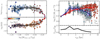 |
Fig. 9. DGR and α12CO(1−0) trends and atomic/molecular gas profiles Left: the trend of α12CO(1−0) and DGR as a function of the log(WCO/ΣH I), which roughly translates to the molecular-to-atomic gas fraction. The points indicate the individual solution pixels. The color indicates the galactocentric radius. The black line indicates the binned trend, and the dark-shaded region shows the 1σ scatter. The vertical dashed line is arbitrarily drawn and shows approximately beyond where the two parameters start to deviate from a flat trend. Right: radial profiles of ΣH I and Σmol at solution pixel scale resolution (∼2 kpc). The line indicates the radially binned values. The bottom panel shows the ratio of molecular to atomic gas mass surface density. The horizontal dotted line indicates unity between the molecular and atomic gas surface density. |
The right panel in Fig. 9 illustrates the radial surface density profiles of the atomic and molecular gas mass. The individual points represent the solution pixels and the colored line indicates the respective radially binned trend. We see that the atomic mass surface density, ΣH I, decreases by ∼0.7 dex toward the central kpc region of the galaxy. For the derivation of the molecular gas mass, Σmol, we account here for the variation in α12CO(1−0) derived from the scatter minimization technique. We see that the molecular gas mass surface density decreases radially outward by ∼1 dex from 2 kpc to 8 kpc. However, when accounting for α12CO(1−0) variation, we also see a depression of the molecular gas mass surface density toward the center by again ∼1 dex. (from 2 kpc inward to 0 kpc). The black trend at the bottom of right panel of Fig. 9 shows the molecular-to-atomic gas mass ratio. We see that the outer regions are more H I-dominated, while H2 becomes increasingly relevant radially inward up to ∼2 kpc. Toward the center of the galaxy, the dominance of H2 over H I seems to decrease again.
4.6. Comparison of DGR and α12CO(1 − 0) trends in M51 and M101
For comparison, we investigate α12CO(1−0) trends in the nearby massive star-forming galaxy M51 (NGC 5194). We estimate the conversion factor in M51 identically to the approach used for M101 as described in Sect. 4.1. We use CO(1–0) data from PAWS (Pety et al. 2013), CO(2–1) from CLAWS (den Brok et al. 2022), H I observations from THINGS (Walter et al. 2008) and dust mass maps using the Draine & Li (2007) model. We note that we do not perform short-spacing corrections for the H I data since, upon visual inspection of the spectra, we find that M51 is less affected by negative bowling issues than the M101 observations. Nonetheless, we caution that we could miss a fraction of the total flux by relying only on short-spacing correction. This would mainly lead to a systematic offset of the α12CO(1−0) values and not affect the overall trend (as discussed in Appendix E). Fig. 10 shows the trend of α12CO(1−0) determined from the scatter minimization technique for both M101 and M51 as a function of galactocentric radius, R21, and R13/12. For reference, we show the α12CO(1−0) map for M51 in Appendix G. Table 4 lists the α12CO(1−0) values for M51 using different binnings.
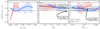 |
Fig. 10. Comparing α12CO(1−0) trends in M101 and M51. Comparison of radial α12CO(1−0) trend in M101(red) and M51(blue). Each panel shows the trend line for both galaxies separately. The trend is determined by binning the α12CO(1−0) values of the individual line of sights. The two dashed lines show the 16th and 84th percentile distribution of the combined M51 and M101 α12CO(1−0) dataset. The shaded region around the trend line shows the respective 1σ scatter of the respective trend line fit. Left: the trend of α12CO(1−0) with galactocentric radius normalized by r25. Center: 12CO line ratio R21 correlation. The thick-dashed line shows a linear regression to the stacked data points (combining M51 and M101). The grey-shaded region between the dotted curves indicates the 1σ confidence interval of the fit. Right: trend with the 13CO-to-12CO line ratio, R13/12. The linear regression only fits the trend for M51 since no clear trend is seen for M101. |
(i) Galactocentric Radius: We do not find any significant trend of α12CO(1−0) with galactocentric radius in M51. Across the disk of the galaxy, we find an average value of  . This is slightly lower but within the scatter margin for the value found by Leroy et al. (2017a). In that study, the authors performed a slightly different version of the scatter minimization technique: they selected a range in α12CO(1−0) that yields a constant DGR trend across the disk of M51. With this technique, they find the following range α12CO(1 − 0)L17 ≈ 4.5 − 5.0 M⊙ pc−2/(K km s−1).
(ii) Line Ratio R21: We reiterate that this particular CO ratio is of interest since it sensitive to variations in density, temperature, and the opacity of the molecular gas (Peñaloza et al. 2017). As the middle panel of Fig. 10 shows, M51 covers higher R21 values than M101. Combining the sightlines from both galaxies, we cover a dynamical range in line ratio values of R21 ∼ 0.5 − 0.9. This range is similar to the full range of line ratio values commonly found across a sample of nearby spiral galaxies (Yajima et al. 2021; Leroy et al. 2022). Given our large uncertainty, we find no significant correlation. The fitted slope is m = −0.5 ± 2. We note that the predicted slope value based on 3D magnetohydrodynamics galaxy-scale simulations of the cloud-scale ISM as given in Gong et al. (2020) is −0.87, which is within our margin of error. In conclusion, despite the range in R21, we do not obtain strong constraints from our observations on any possible trends between the line ratio and the conversion factor. This limits the use of R21 as a predictor of α12CO(1−0) variation for extragalactic studies on kpc scales.
(iii) Line Ratio R13/12: We reiterate that, assuming optically thin 13CO(1–0) emission, R13/12 traces a combination of the 12CO optical depth and abundance variations of the 13CO species (see Sect. 5.1). We expect an optically thin CO line to result in lower α12CO(1−0) values (Bolatto et al. 2013). Consequently, if R13/12 is driven by opacity changes, we expect lower line ratios to have low α12CO(1−0). In Fig. 10, we only perform a linear fit to the trend of M51 since we cover a wider range of line ratios for that galaxy (R13/12 ∼ 0.1 − 0.2). However, given the uncertainties of our α12CO(1−0) values, we do not find any significant trend with R13/12 in M51.
(iv) Arm-interarm variation: As opposed to M101 (see Appendix D), we find strong arm-interarm variation in R21 (Koda et al. 2012; den Brok et al. 2022) in M51, likely reflecting changes in the optical depth or temperature and density of the molecular gas. By decomposing our solution pixels by spiral phase, we can investigate whether α12CO(1−0) shows arm-interarm dependence in M51 as well. Fig. 11 shows α12CO(1−0) binned by spiral phase (spiral phases belonging to the northern spiral arm are shown in red, and blue indicates the spiral phases that define the southern arm; see den Brok et al. 2022 for further details). We decompose the spiral bins using a logarithmic spiral to describe the shape. The technique is described in detail in Koda et al. (2012). We find a significant variation of α12CO(1−0) as a function of the spiral phase. The conversion factor is lower in the interarm than the spiral arm region by about ∼0.5 dex. The arm–interarm trend is consistent with the presence of a more prominent diffuse CO component in the interarm region that enhances the CO emissivity. At the same time, it would decrease the required conversion factor to translate the CO intensity to molecular gas mass. The presence of a diffuse component has previously been suggested by Pety et al. (2013). On the basis of comparing GMC-scale (∼100 pc) and large scale (∼1 kpc) observations, they suggest that ∼50% of the total CO emission could originate from such a diffuse component in this galaxy. Future work using high-resolution observations of the central region of M51 will provide further insight into the mechanism that produces these strong environmental changes in the line ratio and conversion factor (Stuber et al., in prep.). In contrast, we also note that we do not find any clear arm–interarm variation in α12CO(1−0) for M101. We discuss the precise analysis to quantify the arm and interarm regions using logarithmic spirals in Appendix D. We note that since the spiral structure is less pronounced in M101 than in M51, we also expect the difference in R21 to be smaller.
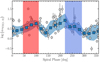 |
Fig. 11. Arm-interarm variation of α12CO(1−0)in M51. The graph shows the 12CO(1–0) intensity binned by spiral phase. The blue points show the stacked line ratio by spiral phases in steps of 20°, increasing counter-clockwise. The vertical red and blue shaded regions show the extent of spiral phases that correspond to the northern (red) and southern (blue) spiral arm of the galaxy. |
5. Discussion
5.1. Implications from CO isotopologue line ratio trends
Generally, CO isotopologue line ratio variation across nearby galaxies is either linked to changes in the relative abundances of the isotopologue species or variation in the physical properties of the molecular gas, such as its opacity, temperature, or density (e.g., Davis 2014). Since the 13CO(1–0) and C18O(1–0) transitions are generally optically thin (see review by Heyer & Dame 2015), they help us to constrain any potential changes in the relative abundances. In more detail, CO isotopologue line ratio variation can generally be explained by the following factors:
(i) Changes in CO isotopologue abundances: Processes that vary the CO isotopologue abundances can be selective nucleosynthesis (Sage et al. 1991; Wilson & Matteucci 1992), chemical fractionation (Watson et al. 1976; Keene et al. 1998) or selective photodissociation (van Dishoeck & Black 1988). These three mechanisms either locally enhance the 13CO abundance (chemical fractionation), increase the 12C and 18O isotope abundances (selective nucleosynthesis), or lead to more photodissociation of certain species due to lower shielding and differences in molecular structure (selective photodissociation). Line ratio trends then give us insight into whether any of these mechanisms act as global drivers and, more importantly, whether abundance variations can explain observed CO isotopologue line ratio trends in the first place. The top left panel in Fig. 12 illustrates the effect of relative abundance variations of 13CO and C18O on the observed line ratio.
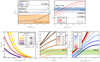 |
Fig. 12. Effect of 13CO optical depth on CO line ratios under LTE (top) and non-LTE (bottom) conditions. We assume optically thick 12CO and optically thin C18O emission. Top left: variation of R18/13 with τ13CO for different abundance ratios of the 13CO and C18O species. We do not significantly detect C18O in the center of the galaxy. The orange shaded region hence shows the region where the line ratio in M101’s central 4 kpc region could fall. Average MW value (solid line; Wouterloot et al. 2008), starburst (dashed line; e.g., Tan et al. 2011), and ULIRGs (dotted; e.g., Greve et al. 2009) is shown. Top right: variation of R13/12 with τ13CO for different beam filling factor ratios between the 12CO and 13CO emission, η12 and η13. The blue band shows the range of measured R13/12 values in M101. Average MW value from Roman-Duval et al. (2016), starburst and ULIRGs from Sliwa & Downes 2017. Bottom panels: we use the line ratio model calculation provided in Leroy et al. (2022). These are based on model calculations with RADEX (van der Tak et al. 2007) and used a lognormal density distributions described in Leroy et al. (2017b). Bottom left: we fix the ratio at R21 = 0.6 and use a lognormal density distribution width of σ = 0.6. The color-coded lines show as a function of H2 volume density (x-axis) and kinetic temperature Tkin (y-axis) the trends for different total CO column densities per line width (NCO/Δν), which roughly correlate with the optical depth. Bottom center: the line ratio R21 as a function of kinetic temperature for different mean molecular gas densities. Bottom right: the line ratio R21 as a function of the mean molecular gas density for different kinetic temperatures. The green shaded region shows the 16th to 84th percentile range for the values found in M101. For the computation of R21 as function of temperature and density, we fix σ = 0.6 dex and NCO/Δv = 1016 cm−2 (km s−1)−1. We note that we assume a common excitation (density, temperature) for all species and LTE for the top panels. |
(ii) Optical depth effects: Because, in particular, the 12CO emission, and potentially the 13CO emission is optically thick, changes in the optical depth will then lead to a variation of the observed line ratio. Due to sufficiently low abundance, C18O generally remains optically thin. This way, it is possible to assess the optical depth variation of 12CO and 13CO.
In Fig. 12 we show the expected R13/12 and R18/13 trends with changing 13CO(1–0) optical depth, τ13CO, under LTE assumption. Since we only derive upper limits for R18/13, the top left panel in Fig. 12 highlights the possible line ratio values up to the upper limit. For optically thin 13CO emission, R18/13 traces the abundance ratio between these two CO isotopologues, X18/13. Our upper limit of the line ratio suggests an upper limit of the abundance ratio of X18/13 < 0.06. The top right panel shows the variation of R13/12 for different beam filling factor ratios for 12CO(1–0) and 13CO(1–0). We note that the observed range in line ratio values found in M101 is in agreement with optically thin 13CO emission (i.e., τ13CO < 1). In the bottom panels of Fig. 12, we illustrate the dependence of R21 on the temperature (kinetic temperature; Tkin) and density (collider density;  ). We use the model calculations from Leroy et al. (2022). They employ multiphase RADEX model calculations (van der Tak et al. 2007) with density layers weighted by a lognormal profile and a common temperature, Tk, and column density per line width, NCO/Δν, (Leroy et al. 2017b). To illustrate the trends, we fix R21 = 0.6 and show the n0, H2-pagination-to-Tkin degeneracy for different CO column densities per line width. We expect the column density per line width to decrease toward the center. Consequently, fixing R21, would indicate an increase of the temperature (for constant density) and higher density (for constant temperature) toward the central region of M101 (or a combination of both effects).
Given optically thin 13CO, the negative trend we find in R13/12 with galactocentric radius either derives from changes in the optical depth of 12CO or changes in the abundance ratio of [12CO/13CO] (or a combination of these two factors). An increase of the X13/12 abundance ratio toward the center would be consistent with such observed trends in the Milky Way (Milam et al. 2005). Such trends can be explained by selective nucleosynthesis: inside-out star formation scenarios (Tang et al. 2019) lead to an increased accumulation of 13CO sooner towards the center of the galaxy, thus enhancing there the R13/12 ratio. Such a scenario is also supported by the increase of R13/12 with the star formation rate surface density (see the bottom right panel in Fig. 5). We note, however, that it remains an open question how precisely the star formation history connects to the abundance of (molecular) gas we observe. To address the connection in the case of M101, higher-resolution observations of the chemical abundance variation on the molecular cloud scale are necessary.
Alternatively, the optical depth of 12CO is expected to decrease in the presence of diffuse emission or increased turbulence. This would boost the emission of 12CO relative to 13CO and lead to a decreasing R13/12. In contrast, the optical depth could also increase if the column density increases towards the center of the galaxy. If changes in the optical depth were the main driver for line ratio variation, the increasing trend of R13/12 toward the center of M101 would indicate higher optical depth in the center. Given our nearly flat R21, higher optical depths would mean less dense or colder molecular gas (as can be seen in Fig. 12). We hence conclude that particularly the trend in R13/12 is in part due to changes in the relative abundance of 13CO. However, for future work to properly disentangle the contribution of abundance variations and optical depth changes to the line ratio, at least another 13CO rotational J transition is required to perform a non-LTE modeling analysis (e.g., Teng et al. 2022).
5.2. Impact of α12CO(1 − 0) variation on scaling relations
The Kennicutt-Schmidt (KS) relation (Schmidt 1959; Kennicutt 1989) links the star formation surface density and the total gas surface density, and its slope likely reflects the underlying processes of star formation (Elmegreen 2002; Krumholz & McKee 2005). The molecular KS law (which relates the SFR surface density to only the molecular gas surface density) follows:
 (14)
(14)
where N indicates the KS slope and C the normalization offset.
When estimating the KS relation from observations, the molecular gas surface density is most often inferred from CO observations. CO (2–1) and CO (1–0) are often used for this purpose, and translating from CO intensity to molecular gas mass surface density requires adopting some CO-to-H2 conversion factor. This means that for the increasingly common set of high-quality CO (2–1) mapping and integrated data (e.g., Cicone et al. 2017; Noble et al. 2019; Pereira-Santaella et al. 2021; Leroy et al. 2021), both the line ratio and adopted 12CO(1–0)-to-H2 conversion factor can affect the derived surface density, scaling relation, and molecular gas depletion time. In this study, we are uniquely positioned to investigate the impact of using either a constant or varying line ratio R21 (i.e., using either 12CO(2–1) and a line ratio, or 12CO(1–0) directly) and conversion factor α12CO(1−0). In Fig. 13, we compare the different derived KS slopes, N, in M101 and M51 based on (i) using 12CO(1–0) and a radially interpolated α12CO(1−0) (ii) 12CO(1–0) and a fixed  , and (iii) 12CO(2–1) and a fixed R21 = 0.6 (and R21 = 0.9 in M51; den Brok et al. 2022) and the same fixed α12CO(1−0) value as for (ii). The points, which show the solution pixels, are color-coded by the difference (in dex) compared to the molecular gas mass derived from 12CO(2–1) according to (iii).
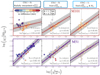 |
Fig. 13. Impact of varying R21 and α12CO(1−0) on the Kennicutt-Schmidt relation We compare the KS relation using three different ways of estimating the molecular gas mass, Σmol: (i) 12CO(1–0) and a radially interpolated α12CO(1−0) derived for each galaxy (ii) 12CO(1–0) and a fixed α12CO(1 − 0)MW = 4.3 M⊙ pc−2/(K km s−1), and (iii) 12CO(2–1) and a fixed R21 = 0.6 (and R21 = 0.9 in M51; den Brok et al. 2022). The resulting KS index, N, is determined using an orthogonal distance regression (fit indicated by solid line) and indicated in each panel with its 1σ uncertainty. In addition, each panel also lists the ΣSFR value (in log) at Σmol = 10 M⊙ pc−2, as derived from the linear fit. The KS coefficient, N, the Pearson’s correlation coefficient, p, and as the SFR surface density at a molecular gas mass surface density of 10 M⊙ pc−2 or the linear relationship are indicated in each panel as well. The grey shaded region shows the ±0.30 dex dispersion which is expected for a larger sample of galaxies (Bigiel et al. 2008; Leroy et al. 2013). The points, which represent the individual solution pixels, are color-coded by their difference (in dex) in Σmol to the molecular gas mass determined using method (iii), which is shown in the right panel. Squares indicate the central points (r ≤ 2 kpc). |
Each panel also indicates the KS index, N (including the 1σ uncertainty shaded in gray). The index is determined using an orthogonal distance regression, which is more robust than the more commonly used linear regression, with x and y as observables with associated uncertainties. The right-most panel shows the relation based on method (iii). We find an index N < 1 for both galaxies. While the KS relation predicts a close relation between ΣSFR and Σmol, an overall dispersion from this relation is expected (±0.30 dex; Bigiel et al. 2008; Leroy et al. 2013) and connected to physical drivers. Regarding free (left and central panels) and fixed (right panels) R21, we find a decrease for M101 (N = 0.76 to N = 0.64), but an increase in N for M51 (N = 0.85 to N = 1.02). We generally expect an increase of the index since R21 becomes larger towards the center, leading to an overestimation of the molecular gas mass (∼difference of 10–20%; Yajima et al. 2021; den Brok et al. 2021; Leroy et al. 2022). We see that in M101, the points with higher ΣSFR (connected to the center) also show a negative (blue) difference in molecular mass. The impact of R21 is limited by its factor of 2 variation because it saturates at 1 and is limited to 0.4 by typical excitation condition (see also. e.g., Yajima et al. 2021; Leroy et al. 2022).
We expect the impact by varying α12CO(1−0) to be larger since we observe a variation of the conversion factor of a factor of 5 − 10. When estimating the molecular gas mass using the radially interpolated α12CO(1−0) value (left column in Fig. 13), we see a further increase in N for M51 and a decrease for M101 compared to using a fixed α12CO(1−0). Since values with higher surface density seem to show a depression of α12CO(1−0) (e.g., the center), we expect that points with higher ΣSFR have overestimated molecular gas masses. Correcting this effect by accounting for α12CO(1−0) variation will push these points to lower Σmol. This can be seen in M101, where the squared points (for which r ≤ 2 kpc) are bluer than for fixed α12CO(1−0). The other high-SFR points stem from the bright H II region toward the southeast. We overestimate Σmol when not accounting for varying R21 and α12CO(1−0)(in particular for the center). We hence expect to find a larger KS slope than if we were accounting for varying α12CO(1−0) and R21. However, we find that a simple KS parameterization is breaking in M101 when accounting for the variation in R21 and α12CO(1−0)(left panels of Fig. 13). This is because (a) the dynamical range in the SFR surface density is small (∼0.5 dex) and (b) the points from the center of the galaxy are pushed off the linear relation (c) the H II region (NGC 5461) at high-SFR shows points offset from the main relation. Hence, a linear fit does not capture the entire trend of the relation.
Furthermore, to study environmental variation, we investigate how the molecular gas depletion time τdep varies as a function of radius across both galaxies. The depletion time is defined as follows:
 (15)
(15)
Figure 14 shows the radial trend of τdep for either fixed R21 and α12CO(1−0), or a radially interpolated α12CO(1−0). Both galaxies show relatively flat depletion times in their discs, independent of the Σmol method. This is in agreement with previous studies of resolved nearby galaxies that also found a relatively narrow distribution of molecular gas depletion time (e.g., Leroy et al. 2008, 2013; Bigiel et al. 2011). Using radial α12CO(1−0) and CO(1–0), we find an average depletion time of  Gyr and
  Gyr with a scatter of 0.2 dex for both galaxies. We also note that the value for the average depletion time in both galaxies agrees well with the value of 1.6 Gyr found for M51 by Leroy et al. (2017a) using PAWS CO(1–0) data and is well within the range expected from varying the choice of SFR tracer. Using the constant α12CO(1−0) and R21, we find a slightly higher depletion time in M51 by about 500 Myr (which constitutes a ∼50% increase). Such constant depletion times are thought to represent evidence that averaging over many GMCs on kpc-scales in the disks of nearby spiral galaxies the SFR per unit gas mass is relatively constant (e.g., Leroy et al. 2008; Bigiel et al. 2011).
 |
Fig. 14. Impact of varying R21 and α12CO(1−0) on the molecular gas depletion time The top panels show the radial trend of the depletion time for M101 (left), M51 (center), and for the combination of the sightlines from both galaxies (right). The depletion time depends on a measurement of the molecular gas mass. The grey points (with purple edge color) show the measurements using CO(2–1) and fixed R21 and α12CO(1−0) values. The points color-coded by SFR surface density are from using CO(1–0) and a radially interpolated α12CO(1−0). The bottom panels compare the radially binned trends of both measurements. The grey line indicates the residual between the two trend lines. |
While M51 shows a narrow range of depletion time across the galaxy, independent of the method used, we see an apparent decrease of τdep toward the center of M101 when we use a radially interpolated α12CO(1−0). In the center, the constant trend seems to break, and we find τdep ≈ 150 − 300 Myr, which is an order of magnitude lower than the disk-wide average. Furthermore, M101 shows lower depletion times (again by almost one order of magnitude) in the bright H II region toward the southeast of the galaxy (NGC 5462). Sightlines within this region incidentally show also high SFR surface densities. Utomo et al. (2017), studying galaxies from the EDGE-CALIFA survey, and Leroy et al. (2013) investigating resolved observations of the HERACLES sample, also found decreased depletion times toward the center of galaxies and suggested that when accounting for α12CO(1−0) variation, the extent of the drop in τdep will be amplified. A possible explanation for the central depression could be low crossing and free-fall times of the clouds in the central region as opposed to clouds in the galactic disks (e.g., Leroy et al. 2015).
5.3. Comparing prescriptions of α12CO(1 − 0)
We compare commonly used α12CO(1−0)-prescriptions to our estimate from the scatter minimization technique in M101 and M51. Such prescriptions are primarily based on first order on the metallicity, Z (e.g., Schruba et al. 2012; Accurso et al. 2017), but also incorporate further key parameters such as the surface brightness (e.g., Bolatto et al. 2013) or the CO line ratio, R21 (e.g., Gong et al. 2020), which traces to some degree also the temperature dependence of the conversion factor. In particular, we test the prescription from Bolatto et al. (2013) and prescription from Accurso et al. (2017; which describes α12CO(1−0) in terms of a power-law scaling with metallicity, similar to Schruba et al. 2012; Amorín et al. 2016). The panels of Fig. 15 show a comparison of the radial trends of α12CO(1−0) for the different prescriptions and the trend based on the scatter minimization technique (shown in color) for M101 (left) and M51 (right). For M101, in the disk, the prescription based on metallicity alone (dotted line; Sun et al. 2020, which is based on the prescription by Accurso et al. 2017) describes the range of α12CO(1−0) approximately well in M101 and is slightly offset in M51 toward larger values (by about 0.3 dex). However, this prescription does not predict the depression of α12CO(1−0) toward the center of the galaxy in M101. In contrast, we see that the prescription by Bolatto et al. (2013), which accounts for regions with high total mass surface density, also describes a mild depression of α12CO(1−0) toward the center of both galaxies. But the extent of the decrease is only ∼0.5 dex with respect to the average disk value, and not ∼1 dex, as we see in M101. The prescription by Bolatto et al. (2013) also finds a decreasing trend toward the centre in M51 (by ∼0.5 dex). This finding suggests that the reason is linked to the peculiarity mentioned above of M51, such as the AGN in the center or its strong interaction with the companion galaxy NGC 5195.
 |
Fig. 15. CO(1–0)-to-H2 conversion factor prescription comparison Comparing the radial α12CO(1−0) trend derived from binning the data (in color) and the trend derived from applying different prescriptions. The trend for M101 is shown in the left and for M51 on the right. Comparison of the derived trend when applying the α12CO(1−0) prescription used Sun et al. (2022; dotted line), from Bolatto et al. (2013; dash-dotted line). The black horizontal line illustrates the average local solar neighborhood α12CO(1−0) value. The green-shaded region is an approximate illustration of the central region of the galaxy, where conditions potentially change dramatically to the overall disk. |
6. Conclusions
This study presents new wide-field IRAM 30 m low-J CO observations of M101. We address two key aspects of studies of the molecular gas physics in the galaxies M101 and M51: i) How well do CO isotopologue line emissions capture changes in the molecular gas characteristics, and ii) how does α12CO(1−0) vary with environmental parameters across the galaxy.
Based on our CO isotopologue analysis, we find:
-
An average line ratio of
 , which is consistent with previous studies of similar, nearby star-forming galaxies. The ratio stays predominantly flat across the disk of M101, with only a mild increase of 10% towards the central 1.5 kpc region.
 -
We also detect resolved 13CO(1–0) emission across the center, bar end, and spiral arm of M101. We find an average 13CO/12CO(1–0) line ratio of
 , which suggests optically thin 13CO emission throughout the galaxy.
 -
Using spectral stacking, we can constrain an upper limit for R18/13 < 0.07 for the central 4 kpc region (by radius). Such low line ratios are more predominantly found in the outskirts of star-forming galaxies and indicate very low relative abundances of the C18O species.
-
Given the observed trend in R13/12, which increases toward the center, we conclude that changes in abundances due to nucleosynthesis are a major driver on galaxy-wide scales. Changes in the opacity of 12CO do not seem to be the primary driver, since the optical depth generally decreases toward the center, which would result in an opposite R13/12 trend.
Besides this in-depth analysis of the 3 mm CO isotopologue line ratios, we investigate the variation of the CO-to-H2 conversion factor, α12CO(1−0) across M101. We use a modified version of the scatter minimization technique. The method is based on the dust mass approach, and we use both the 12CO(1–0) and (2–1) emission lines to estimate αCO(1 − 0). Our main results and conclusion can be summarized as follows:
-
We find an average conversion factor of ⟨α12CO(1 − 0)⟩ = 4.4 ± 0.9 across the disk of galaxy M101, with an apparent decrease of the value towards the galaxy’s center by a factor of ∼10. The reduction of the conversion factor towards the center of the galaxy follows the qualitative expectation that the turbulence increases, hence decreasing the optical depth, which enhances the 12CO emission. We note however, that such conditions are usually more expected in the starburst regime than in the center of regular disk galaxies. For comparison, we also perform a scatter minimization approach in M51. We find a relatively flat α12CO(1−0) trend in M51 across the disk and center of the galaxy.
-
Using the optically thin 13CO emission, we perform an LTE-based α12CO(1−0) estimation in M101. Generally, the conversion factor determined using this approach is lower by a factor 2 − 3 compared to the scatter minimization technique. The discrepancy is likely due to the simplifying assumption of a similar beam-filling factor of the two lines, using constant excitation temperature and a change in the relative abundance of the species. In general, the variation of all three assumptions is plausible. As a consistency check, we introduce a two-component model of a galaxy and change the conditions in the center and disk. We derive a depression of α12CO(1 − 0)LTE of similar order as the scatter minimization derived α12CO(1−0), showing that the depression is plausible under the set of assumptions.
-
Compared to the results one would obtain assuming a fixed α12CO(2 − 1), one significantly overestimates the molecular gas mass, particularly in the center of galaxies. We find that, in particular, for M101, the simple linear Kennicutt Schmidt relation breaks if accounting for variable α12CO(1−0). In addition, we find that the molecular gas depletion time seems to be significantly overestimated in the center by ∼1 dex with respect to depletion time of 1.9 Gyr across the disk, if not accounting for α12CO(1−0) variation. In contrast, M51 shows a depletion time of 1.5 Gyr, without a radial trend.
-
Finding a prescription for α12CO(1−0) on kpc-scale remains challenging. For M101 and M51, commonly used prescriptions yield estimates of the conversion factor for the central kpc-regions that are off by > 0.5 dex. While M101 shows a stronger depression of α12CO(1−0) than predicted, M51 does not show any decrease toward the center, despite being predicted by the prescription.
Overall, our results shed new light on the degree of variation of α12CO(1−0) and the corresponding trends with key galactic properties. In particular, we stress that the points near the galaxy centers need to be treated with care when employing commonly used α12CO(1−0) prescriptions, as the depression of the central value is not yet fully captured or understood. With future higher-resolution CO isotopologue observations of molecular clouds in the center and disk of nearby star-forming galaxies, it will become possible to address the physical conditions of the molecular gas that can explain the depression in α12CO(1−0).
https://uvcombine.readthedocs.io/en/latest/
We use a sigmoid function with an arbitrary width to vary the conditions smoothly between disk and center. We do this to simulate a more realistic transition between the two phases. In our case, we set the width of the sigmoid to the width of a solution pixel (∼2 kpc).
Acknowledgments
JdB, FB, JP and ATB acknowledge funding from the European Research Council (ERC) under the European Union’s Horizon 2020 research and innovation programme (grant agreement No.726384/Empire). JdB and EWK acknowledge support from the Smithsonian Institution as a Submillimeter Array (SMA) Fellow. JC acknowledges support from ERC starting grant #851622 DustOrigin. KS was supported by NSF award 2108081. The work of AKL is partially supported by the National Science Foundation under Grants No. 1615105, 1615109, and 1653300. AU acknowledges support from the Spanish grants PGC2018-094671-B-I00, funded by MCIN/AEI/10.13039/501100011033 and by “ERDF A way of making Europe”, and PID2019-108765GB-I00, funded by MCIN/AEI/10.13039/501100011033. ES and TGW acknowledge funding from the European Research Council (ERC) under the European Union’s Horizon 2020 research and innovation programme (grant agreement No. 694343). ER acknowledges the support of the Natural Sciences and Engineering Research Council of Canada (NSERC), funding reference number RGPIN-2022-03499. IC acknowledges the National Science and Technology Counsil for support through grants 108-2112-M-001-007-MY3 and 111-2112-M-001-038-MY3, and the Academia Sinica for Investigator Award AS-IA-109-M02. TS acknowledges funding from the European Research Council (ERC) under the European Union’s Horizon 2020 research and innovation programme (grant agreement No. 694343). MC gratefully acknowledges funding from the Deutsche Forschungsgemeinschaft (DFG) through an Emmy Noether Research Group, grant number CH2137/1-1. COOL Research DAO is a Decentralized Autonomous Organization supporting research in astrophysics aimed at uncovering our cosmic origins. CE acknowledges funding from the Deutsche Forschungsgemeinschaft (DFG) Sachbeihilfe, grant number BI1546/3-1. SCOG acknowledges support from the DFG via SFB 881 “The Milky Way System” (sub-projects B1, B2 and B8) and from the Heidelberg cluster of excellence EXC 2181-390900948 “STRUCTURES: A unifying approach to emergent phenomena in the physical world, mathematics, and complex data,” funded by the German Excellence Strategy. Y-HT acknowledges funding support from NRAO Student Observing Support Grant SOSPADA-012 and from the National Science Foundation (NSF) under grant No. 2108081.
References
- Abdeen, S., Kennefick, D., Kennefick, J., et al. 2020, MNRAS, 496, 1610 [NASA ADS] [CrossRef] [Google Scholar]
- Accurso, G., Saintonge, A., Catinella, B., et al. 2017, MNRAS, 470, 4750 [NASA ADS] [Google Scholar]
- Ahumada, R., Prieto, C. A., Almeida, A., et al. 2020, ApJS, 249, 3 [Google Scholar]
- Alatalo, K., Crocker, A. F., Aalto, S., et al. 2015, MNRAS, 450, 3874 [Google Scholar]
- Amorín, R., Muñoz-Tuñón, C., Aguerri, J. A. L., & Planesas, P. 2016, A&A, 588, A23 [NASA ADS] [CrossRef] [EDP Sciences] [Google Scholar]
- Anand, G. S., Lee, J. C., Van Dyk, S. D., et al. 2021, MNRAS, 501, 3621 [Google Scholar]
- Berg, D. A., Skillman, E. D., Croxall, K. V., et al. 2015, ApJ, 806, 16 [NASA ADS] [CrossRef] [Google Scholar]
- Berg, D. A., Pogge, R. W., Skillman, E. D., et al. 2020, ApJ, 893, 96 [NASA ADS] [CrossRef] [Google Scholar]
- Bigiel, F., Leroy, A., Walter, F., et al. 2008, AJ, 136, 2846 [NASA ADS] [CrossRef] [Google Scholar]
- Bigiel, F., Leroy, A. K., Walter, F., et al. 2011, ApJ, 730, L13 [NASA ADS] [CrossRef] [Google Scholar]
- Blanton, M. R., Bershady, M. A., Abolfathi, B., et al. 2017, AJ, 154, 28 [Google Scholar]
- Bolatto, A. D., Wolfire, M., & Leroy, A. K. 2013, ARA&A, 51, 207 [CrossRef] [Google Scholar]
- Brown, T., & Wilson, C. D. 2019, ApJ, 879, 17 [NASA ADS] [CrossRef] [Google Scholar]
- Cao, Y., Wong, T., Xue, R., et al. 2017, ApJ, 847, 33 [NASA ADS] [CrossRef] [Google Scholar]
- Casasola, V., Cassarà, L. P., Bianchi, S., et al. 2017, A&A, 605, A18 [NASA ADS] [CrossRef] [EDP Sciences] [Google Scholar]
- Chastenet, J., Sandstrom, K., Chiang, I.-D., et al. 2021, ApJ, 912, 103 [NASA ADS] [CrossRef] [Google Scholar]
- Chiang, I.-D., Sandstrom, K. M., Chastenet, J., et al. 2018, ApJ, 865, 117 [NASA ADS] [CrossRef] [Google Scholar]
- Cicone, C., Bothwell, M., Wagg, J., et al. 2017, A&A, 604, A53 [NASA ADS] [CrossRef] [EDP Sciences] [Google Scholar]
- Clark, C. J. R., Schofield, S. P., Gomez, H. L., & Davies, J. I. 2016, MNRAS, 459, 1646 [NASA ADS] [CrossRef] [Google Scholar]
- Clark, C. J. R., De Vis, P., Baes, M., et al. 2019, MNRAS, 489, 5256 [NASA ADS] [CrossRef] [Google Scholar]
- Cormier, D., Bigiel, F., Jiménez-Donaire, M. J., et al. 2018, MNRAS, 475, 3909 [NASA ADS] [CrossRef] [Google Scholar]
- Croxall, K. V., Pogge, R. W., Berg, D. A., Skillman, E. D., & Moustakas, J. 2016, ApJ, 830, 4 [NASA ADS] [CrossRef] [Google Scholar]
- Dalcanton, J. J., Fouesneau, M., Hogg, D. W., et al. 2015, ApJ, 814, 3 [Google Scholar]
- Dale, D. A., Cohen, S. A., Johnson, L. C., et al. 2009, ApJ, 703, 517 [Google Scholar]
- Davis, T. A. 2014, MNRAS, 445, 2378 [NASA ADS] [CrossRef] [Google Scholar]
- den Brok, J. S., Chatzigiannakis, D., Bigiel, F., et al. 2021, MNRAS, 504, 3221 [NASA ADS] [CrossRef] [Google Scholar]
- den Brok, J. S., Bigiel, F., Sliwa, K., et al. 2022, A&A, 662, A89 [CrossRef] [EDP Sciences] [Google Scholar]
- Downes, D., & Solomon, P. M. 1998, ApJ, 507, 615 [NASA ADS] [CrossRef] [Google Scholar]
- Draine, B. T., & Li, A. 2007, ApJ, 657, 810 [CrossRef] [Google Scholar]
- Dwek, E. 1998, ApJ, 501, 643 [NASA ADS] [CrossRef] [Google Scholar]
- Eibensteiner, C., Barnes, A. T., Bigiel, F., et al. 2022, A&A, 659, A173 [CrossRef] [EDP Sciences] [Google Scholar]
- Elmegreen, B. G. 2002, ApJ, 577, 206 [CrossRef] [Google Scholar]
- Fazio, G. G., Hora, J. L., Allen, L. E., et al. 2004, ApJS, 154, 10 [Google Scholar]
- Frisch, P. C., & Slavin, J. D. 2003, ApJ, 594, 844 [CrossRef] [Google Scholar]
- Glover, S. C. O., & Clark, P. C. 2016, MNRAS, 456, 3596 [Google Scholar]
- Glover, S. C. O., & Mac Low, M. M. 2011, MNRAS, 412, 337 [NASA ADS] [CrossRef] [Google Scholar]
- Gong, M., Ostriker, E. C., Kim, C.-G., & Kim, J.-G. 2020, ApJ, 903, 142 [CrossRef] [Google Scholar]
- Gordon, K. D., Roman-Duval, J., Bot, C., et al. 2014, ApJ, 797, 85 [NASA ADS] [CrossRef] [Google Scholar]
- Greve, T. R., Papadopoulos, P. P., Gao, Y., & Radford, S. J. E. 2009, ApJ, 692, 1432 [Google Scholar]
- Griffin, M. J., Abergel, A., Abreu, A., et al. 2010, A&A, 518, L3 [EDP Sciences] [Google Scholar]
- Heiderman, A., Evans, N. J. I., Allen, L. E., Huard, T., & Heyer, M. 2010, ApJ, 723, 1019 [Google Scholar]
- Henkel, C., Wilson, T. L., Langer, N., Chin, Y. N., & Mauersberger, R. 1994, Interstellar CNO Isotope Ratios, (Springer), 439, 72 [NASA ADS] [Google Scholar]
- Heyer, M., & Dame, T. M. 2015, ARA&A, 53, 583 [Google Scholar]
- Israel, F. P. 1997, A&A, 328, 471 [NASA ADS] [Google Scholar]
- Israel, F. P. 2009a, A&A, 493, 525 [NASA ADS] [CrossRef] [EDP Sciences] [Google Scholar]
- Israel, F. P. 2009b, A&A, 506, 689 [NASA ADS] [CrossRef] [EDP Sciences] [Google Scholar]
- Israel, F. P. 2020, A&A, 635, A131 [NASA ADS] [CrossRef] [EDP Sciences] [Google Scholar]
- Jenkins, E. B. 2009, ApJ, 700, 1299 [Google Scholar]
- Jiménez-Donaire, M. J., Cormier, D., Bigiel, F., et al. 2017, ApJ, 836, L29 [Google Scholar]
- Jiménez-Donaire, M. J., Bigiel, F., Leroy, A. K., et al. 2019, ApJ, 880, 127 [CrossRef] [Google Scholar]
- Kamenetzky, J., Rangwala, N., Glenn, J., Maloney, P. R., & Conley, A. 2014, ApJ, 795, 174 [Google Scholar]
- Keene, J., Schilke, P., Kooi, J., et al. 1998, ApJ, 494, L107 [NASA ADS] [CrossRef] [Google Scholar]
- Kennicutt, R. C., Jr 1989, ApJ, 344, 685 [CrossRef] [Google Scholar]
- Kennicutt, R. C., Jr, Bresolin, F., & Garnett, D. R. 2003, ApJ, 591, 801 [NASA ADS] [CrossRef] [Google Scholar]
- Kennicutt, R. C., Calzetti, D., Aniano, G., et al. 2011, PASP, 123, 1347 [Google Scholar]
- Koch, E. W., Rosolowsky, E. W., Lockman, F. J., et al. 2018, MNRAS, 479, 2505 [NASA ADS] [CrossRef] [Google Scholar]
- Koda, J., Scoville, N., Hasegawa, T., et al. 2012, ApJ, 761, 41 [NASA ADS] [CrossRef] [Google Scholar]
- Köhler, M., Ysard, N., & Jones, A. P. 2015, A&A, 579, A15 [NASA ADS] [CrossRef] [EDP Sciences] [Google Scholar]
- Kramer, C., Peñalver, J., & Greve, A. 2013, Improvement of the IRAM 30 m Telescope Beam Pattern, Tech. Rep. 2013-1 [Google Scholar]
- Krumholz, M. R., & McKee, C. F. 2005, ApJ, 630, 250 [Google Scholar]
- Langer, W. D., & Penzias, A. A. 1993, ApJ, 408, 539 [NASA ADS] [CrossRef] [Google Scholar]
- Leroy, A. K., Bolatto, A., Stanimirovic, S., et al. 2007, ApJ, 658, 1027 [NASA ADS] [CrossRef] [Google Scholar]
- Leroy, A. K., Walter, F., Brinks, E., et al. 2008, AJ, 136, 2782 [Google Scholar]
- Leroy, A. K., Walter, F., Bigiel, F., et al. 2009, AJ, 137, 4670 [Google Scholar]
- Leroy, A. K., Bolatto, A., Gordon, K., et al. 2011, ApJ, 737, 12 [Google Scholar]
- Leroy, A. K., Walter, F., Sandstrom, K., et al. 2013, AJ, 146, 19 [Google Scholar]
- Leroy, A. K., Bolatto, A. D., Ostriker, E. C., et al. 2015, ApJ, 801, 25 [NASA ADS] [CrossRef] [Google Scholar]
- Leroy, A. K., Schinnerer, E., Hughes, A., et al. 2017a, ApJ, 846, 71 [Google Scholar]
- Leroy, A. K., Usero, A., Schruba, A., et al. 2017b, ApJ, 835, 217 [NASA ADS] [CrossRef] [Google Scholar]
- Leroy, A. K., Sandstrom, K. M., Lang, D., et al. 2019, ApJS, 244, 24 [Google Scholar]
- Leroy, A. K., Schinnerer, E., Hughes, A., et al. 2021, ApJS, 257, 43 [NASA ADS] [CrossRef] [Google Scholar]
- Leroy, A. K., Rosolowsky, E., Usero, A., et al. 2022, ApJ, 927, 149 [NASA ADS] [CrossRef] [Google Scholar]
- Lodders, K. 2003, ApJ, 591, 1220 [Google Scholar]
- Lodders, K. 2010, Astrophys. Space Sci. Proc., 16, 379 [NASA ADS] [CrossRef] [Google Scholar]
- Maloney, P., & Black, J. H. 1988, ApJ, 325, 389 [NASA ADS] [CrossRef] [Google Scholar]
- Mangum, J. G., Emerson, D. T., & Greisen, E. W. 2007, A&A, 474, 679 [NASA ADS] [CrossRef] [EDP Sciences] [Google Scholar]
- Martin, D. C., Fanson, J., Schiminovich, D., et al. 2005, ApJ, 619, L1 [Google Scholar]
- Meier, D. S., & Turner, J. L. 2004, AJ, 127, 2069 [CrossRef] [Google Scholar]
- Meier, D. S., Turner, J. L., & Beck, S. C. 2001, AJ, 122, 1770 [NASA ADS] [CrossRef] [Google Scholar]
- Milam, S. N., Savage, C., Brewster, M. A., Ziurys, L. M., & Wyckoff, S. 2005, ApJ, 634, 1126 [Google Scholar]
- Mok, A., Wilson, C. D., Knapen, J. H., et al. 2017, MNRAS, 467, 4282 [NASA ADS] [CrossRef] [Google Scholar]
- Narayanan, D., Krumholz, M. R., Ostriker, E. C., & Hernquist, L. 2012, MNRAS, 421, 3127 [NASA ADS] [CrossRef] [Google Scholar]
- Noble, A. G., Muzzin, A., McDonald, M., et al. 2019, ApJ, 870, 56 [Google Scholar]
- Paglione, T. A. D., Wall, W. F., Young, J. S., et al. 2001, ApJS, 135, 183 [NASA ADS] [CrossRef] [Google Scholar]
- Paradis, D., Bernard, J. P., & Mény, C. 2009, A&A, 506, 745 [NASA ADS] [CrossRef] [EDP Sciences] [Google Scholar]
- Paturel, G., Petit, C., Prugniel, P., et al. 2003, A&A, 412, 45 [NASA ADS] [CrossRef] [EDP Sciences] [Google Scholar]
- Peñaloza, C. H., Clark, P. C., Glover, S. C. O., Shetty, R., & Klessen, R. S. 2017, MNRAS, 465, 2277 [CrossRef] [Google Scholar]
- Pereira-Santaella, M., Colina, L., García-Burillo, S., et al. 2021, A&A, 651, A42 [NASA ADS] [CrossRef] [EDP Sciences] [Google Scholar]
- Pety, J., Schinnerer, E., Leroy, A. K., et al. 2013, ApJ, 779, 43 [NASA ADS] [CrossRef] [Google Scholar]
- Pilbratt, G. L., Riedinger, J. R., Passvogel, T., et al. 2010, A&A, 518, L1 [NASA ADS] [CrossRef] [EDP Sciences] [Google Scholar]
- Pineda, J. L., Stutzki, J., Buchbender, C., et al. 2020, ApJ, 900, 132 [NASA ADS] [CrossRef] [Google Scholar]
- Planck Collaboration XXI. 2011, A&A, 536, A21 [NASA ADS] [CrossRef] [EDP Sciences] [Google Scholar]
- Planck Collaboration Int. XVII. 2014, A&A, 566, A55 [NASA ADS] [CrossRef] [EDP Sciences] [Google Scholar]
- Planck Collaboration Int. XXII. 2015, A&A, 576, A107 [NASA ADS] [CrossRef] [EDP Sciences] [Google Scholar]
- Poglitsch, A., Waelkens, C., Geis, N., et al. 2010, A&A, 518, L2 [NASA ADS] [CrossRef] [EDP Sciences] [Google Scholar]
- Prantzos, N., Aubert, O., & Audouze, J. 1996, A&A, 309, 760 [NASA ADS] [Google Scholar]
- Puschnig, J., Hayes, M., Östlin, G., et al. 2020, A&A, 644, A10 [NASA ADS] [CrossRef] [EDP Sciences] [Google Scholar]
- Rebolledo, D., Wong, T., Xue, R., et al. 2015, ApJ, 808, 99 [NASA ADS] [CrossRef] [Google Scholar]
- Rieke, G. H., Young, E. T., Engelbracht, C. W., et al. 2004, ApJS, 154, 25 [Google Scholar]
- Roman-Duval, J., Gordon, K. D., Meixner, M., et al. 2014, ApJ, 797, 86 [NASA ADS] [CrossRef] [Google Scholar]
- Roman-Duval, J., Heyer, M., Brunt, C. M., et al. 2016, ApJ, 818, 144 [NASA ADS] [CrossRef] [Google Scholar]
- Roueff, A., Gerin, M., Gratier, P., et al. 2021, A&A, 645, A26 [NASA ADS] [CrossRef] [EDP Sciences] [Google Scholar]
- Sage, L. J., Mauersberger, R., & Henkel, C. 1991, A&A, 249, 31 [NASA ADS] [Google Scholar]
- Saintonge, A., Catinella, B., Tacconi, L. J., et al. 2017, ApJS, 233, 22 [Google Scholar]
- Sandstrom, K. M., Leroy, A. K., Walter, F., et al. 2013, ApJ, 777, 5 [Google Scholar]
- Sawada, T., Hasegawa, T., Handa, T., et al. 2001, ApJS, 136, 189 [NASA ADS] [CrossRef] [Google Scholar]
- Schmidt, M. 1959, ApJ, 129, 243 [NASA ADS] [CrossRef] [Google Scholar]
- Schruba, A., Leroy, A. K., Walter, F., et al. 2012, AJ, 143, 138 [NASA ADS] [CrossRef] [Google Scholar]
- Schruba, A., Leroy, A. K., Kruijssen, J. M. D., et al. 2017, ApJ, 835, 278 [NASA ADS] [CrossRef] [Google Scholar]
- Shetty, R., Vogel, S. N., Ostriker, E. C., & Teuben, P. J. 2007, ApJ, 665, 1138 [NASA ADS] [CrossRef] [Google Scholar]
- Sliwa, K., & Downes, D. 2017, A&A, 604, A2 [NASA ADS] [CrossRef] [EDP Sciences] [Google Scholar]
- Sliwa, K., Wilson, C. D., Aalto, S., & Privon, G. C. 2017, ApJ, 840, L11 [Google Scholar]
- Sofue, Y., Tutui, Y., Honma, M., et al. 1999, ApJ, 523, 136 [NASA ADS] [CrossRef] [Google Scholar]
- Sun, J., Leroy, A. K., Schinnerer, E., et al. 2020, ApJ, 901, L8 [NASA ADS] [CrossRef] [Google Scholar]
- Sun, J., Leroy, A. K., Rosolowsky, E., et al. 2022, ApJ, 164, 43 [CrossRef] [Google Scholar]
- Szũcs, L., Glover, S. C. O., & Klessen, R. S. 2016, MNRAS, 460, 82 [CrossRef] [Google Scholar]
- Tan, Q.-H., Gao, Y., Zhang, Z.-Y., & Xia, X.-Y. 2011, Res. Astron. Astrophys., 11, 787 [CrossRef] [Google Scholar]
- Tang, X. D., Henkel, C., Menten, K. M., et al. 2019, A&A, 629, A6 [NASA ADS] [CrossRef] [EDP Sciences] [Google Scholar]
- Teng, Y.-H., Sandstrom, K. M., Sun, J., et al. 2022, ApJ, 925, 72 [NASA ADS] [CrossRef] [Google Scholar]
- Thronson, H. A., Jr, Hunter, D. A., Telesco, C. M., Greenhouse, M., & Harper, D. A. 1988, ApJ, 334, 605 [CrossRef] [Google Scholar]
- Timmes, F. X., Woosley, S. E., & Weaver, T. A. 1995, ApJS, 98, 617 [NASA ADS] [CrossRef] [Google Scholar]
- Utomo, D., Bolatto, A. D., Wong, T., et al. 2017, ApJ, 849, 26 [NASA ADS] [CrossRef] [Google Scholar]
- van der Tak, F. F. S., Black, J. H., Schöier, F. L., Jansen, D. J., & van Dishoeck, E. F. 2007, A&A, 468, 627 [NASA ADS] [CrossRef] [EDP Sciences] [Google Scholar]
- van Dishoeck, E. F., & Black, J. H. 1988, ApJ, 334, 771 [Google Scholar]
- Waller, W. H., Bohlin, R. C., Cornett, R. H., et al. 1997, ApJ, 481, 169 [NASA ADS] [CrossRef] [Google Scholar]
- Walter, F., Brinks, E., de Blok, W. J. G., et al. 2008, AJ, 136, 2563 [Google Scholar]
- Watson, W. D., Anicich, V. G., & Huntress, W. T., Jr 1976, ApJ, 205, L165 [NASA ADS] [CrossRef] [Google Scholar]
- Werner, M. W., Roellig, T. L., Low, F. J., et al. 2004, ApJS, 154, 1 [NASA ADS] [CrossRef] [Google Scholar]
- Whitworth, A. P., & Jaffa, S. E. 2018, A&A, 611, A20 [NASA ADS] [CrossRef] [EDP Sciences] [Google Scholar]
- Williams, T. G., Gear, W. K., & Smith, M. W. L. 2019, MNRAS, 483, 5135 [NASA ADS] [CrossRef] [Google Scholar]
- Wilson, T. L., & Matteucci, F. 1992, A&ARv, 4, 1 [Google Scholar]
- Winkel, B., Kerp, J., Flöer, L., et al. 2016, A&A, 585, A41 [NASA ADS] [CrossRef] [EDP Sciences] [Google Scholar]
- Wolfire, M. G., Hollenbach, D., & McKee, C. F. 2010, ApJ, 716, 1191 [Google Scholar]
- Wouterloot, J. G. A., Henkel, C., Brand, J., & Davis, G. R. 2008, A&A, 487, 237 [NASA ADS] [CrossRef] [EDP Sciences] [Google Scholar]
- Wright, E. L., Eisenhardt, P. R. M., Mainzer, A. K., et al. 2010, AJ, 140, 1868 [Google Scholar]
- Yajima, Y., Sorai, K., Miyamoto, Y., et al. 2021, PASJ, 73, 257 [NASA ADS] [CrossRef] [Google Scholar]
- Zhang, Z.-Y., Romano, D., Ivison, R. J., Papadopoulos, P. P., & Matteucci, F. 2018, Nature, 558, 260 [Google Scholar]
Appendix A: Single dish scale factor estimation
The scatter minimization technique uses total gas mass estimates derived from dust mass measurements. With the help of atomic gas mass estimates via H I observations, we can separate the total gas in to an atomic and a molecular gas component, from which we can deduce α12CO(1−0). For the analysis, we use H I 21cm cubes from the THINGS survey (Walter et al. 2008). The observations for M101 are, however limited by filtering issues (see Fig. A.1; in Appendix E, the effect when using the H I data that have not been short-space corrected is computed). In order to correct these issues, we feathered the data using H I observations from the Effelsberg-Bonn HI Survey (EBHIS; Winkel et al. 2016).
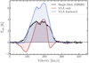 |
Fig. A.1. H I SHORT SPACING CORRECTION The THINGS H I data cube for M101 is seriously affected by filtering and bowling artifacts. The red spectrum illustrates the spectrum for an arbitrarily selected line of sight at 650′ spatial resolution (angular resolution of the Effelsberg single-dish data). The black spectrum shows the same sightline spectrum obtained from the Effelsberg single-dish data (EBHIS survey). We used the uvcombine package to determine a single-dish scale factor of 1.7. The blue spectrum shows the resulting feathered observation for the selected sightline. |
Figure A.1 illustrates the need for correctly feathering the interferometric VLA data from the THINGS survey. The red spectrum indicates the VLA-only data. Clear bowling on both sides of the spectral line seriously hampers integrated intensity measurements. The black spectrum shows the single-dish data in the figure. Using the Python package uvcombine6 we determine a single-dish factor of 1.7 by comparing the flux on scales sampled in both the VLA and EBHIS data sets (see Appendix A in Koch et al. 2018). We use the casa-feather tool to feather the data. Not correcting the VLA-only data would significantly underestimate the total H I emission (total intensity lower by 70% before feathering).
Appendix B: Censored line ratio regions
As a consequence of how we have constructed the line ratio (fainter lines in the numerator), we can also estimate the censored region in the ratio plane. If we observe lines observed with different sensitivity, the noise levels will differ for each line. Since we compare lines of varying brightness, we will obtain many upper limits. We expect to obtain significantly fewer line ratios at lower values since the line in the numerator has reached the sensitivity. Larger line ratios are still possible because this can happen due to either lower line brightness in the denominator (since we have not yet reached the sensitivity limit) or larger brightness of the line in the numerator. We bin the line ratios by a certain quantity. We then estimate the censored 1σ (or 3σ) region in the following way: we divide the average rms (or 3× this value) of the faint line per bin by the average brightness temperature of the brighter line. We reiterate that this approach is only valid when constructing the line ratio to have the fainter line in the numerator. Since rms and the line brightness vary across the survey field, we expect to find a certain number of significantly detected data points within the censored region.
Appendix C: CO Line Stacks
In order to improve the S/N – which allows for the detection of fainter emission lines – we stack the spectra after binning by a certain quantity (e.g., radius, star formation rate surface density, etc.). By shifting the spectrum of each line of sight to the zero velocity, we ensure that the spectra are added coherently. In general, the combination of N independent sightlines will enhance the S/N by a factor  .
.
Figure shows the individual radial stacks for the 12CO(1–0) and 13CO(1–0) molecular transition lines. Each panel indicates the S/N ratio for the integrated 13CO(1–0) intensity. We require a detection with S/N > 3 to classify it as significant. Significant stacks are shown in green, while non-significant line detections are framed in red. We note that with the help of stacking, we do significantly detect 13CO(1–0) out to 8 kpc (i.e., second to last bin).
When we perform radial stacking (with a bin with of ∼ 1.3 kpc), we still do not recover a significant detection of C18O(1–0). However, we detect significant emission in our data if we stack over a larger part of the galaxy. When we stack over the full 12CO(1–0) mask (illustrated by the solid contour in Fig. C.2), we do not find significant line emission. But in contrast, if we stack over the 13CO(1–0) mask (illustrated by the dashed contour line), we detect C18O(1–0) emission with S/N = 3. This detection is valuable since it provides a constraint on the  line intensity ratio. Since both these lines are optically thin, that particular line ratio traces the relative abundance ratio of the two CO isotopologues.
 |
Fig. C.1. Radially stacked 12CO(1–0) (orange) and 13CO(1–0) (purple) spectra. For a better comparison, we scale the 13CO(1–0) brightness temperature up by a factor 5. The S/N of the 13CO(1–0) is indicated in each panel (green indicates spectra where S/N13 > 5. We stack in radial bins of size 1.25 kpc. The shaded region indicates the spectral range over which we integrate the spectra. We detect significant 13CO(1–0) emission out to rgal ∼ 8 kpc. |
 |
Fig. C.2. Stacked CO spectra over the full galaxy (Left) Stacked spectra over the 12CO(1–0) 3σ mask. 13CO(1–0) spectrum scaled up by a factor of 5, C18O(1–0) by a factor of 10. We mark the number of sightlines per mask with n. (Middle) Similar to the left panel, but stacked over the 13CO(1–0) 3σ mask. We do not detected significant C18O(1–0) emission. (Right) moment 0 map of 12CO(1–0). The S/N = 3 contour of 12CO(1–0) is illustrated by the solid line, while for 13CO(1–0) it is indicated by the dashed line. |
Appendix D: Azimuthal variation in M101
Koda et al. (2012) provide a prescription of decomposing sightlines by their corresponding spiral phase. We can bin the data using a logarithmic spiral of the following form:
 (D.1)
(D.1)
where R indicates the galactocentric radius distance of a selected point, k = tan(θ) encapsulates the galaxy’s pitch angle θ, and ψ describes the spiral phase. For M51, we use a pitch angle of θ = 20°, which is close to the values found by Shetty et al. (2007) (θ = 21° .1) and Pineda et al. (2020) (θ = 18° .5).
The spiral arms in M51 could be described using two components: a northern and a southern spiral arm (see Fig. 11). In the case of M101, however, we opted for four spiral arms. We use a pitch angle θM101 = 23° (Abdeen et al. 2020). Fig. D.1 shows the spiral phases (left and central panel) as well as the decomposition of R21 (right panel). We bin the data by segments that span over 40°, and we increment in steps of Δψ = 20°. The phase angle increase in a counterclockwise direction. We find a slightly higher line ratio between spiral arms 3 and 4 (R21 ∼ 0.7). But generally, we do not find any significant arm or interarm variation.
 |
Fig. D.1. Azimuthal Variation of R21 in M101. (Left) The 12CO(1–0) integrated intensity map with the logarithmic spirals with a pitch angle of θ = 23° overlayed. The spirals increment with a spiral phase Δψ = 20° and increment in the counterclockwise direction. The spiral bins have a with of 40°. The thick cyan line indicates ψ = 0. The four spiral arms are accordingly labeled and colored in red. For the spiral binning, we exclude the central 80′ (in diameter), belonging to the central region of the galaxy (indicated by the golden-hatched region in the middle). (Center) The map shows the R21 variation across the galaxy. Spiral bins follow the description on the left panel. (Right) The line ratio is binned by the spiral phase. The gray-shaded region shows the 1σ scatter per bin. The red-shaded region indicates the spiral phases of a particular spiral arm. |
Appendix E: Different Data Sets
The galaxy M101 is also amongst the galaxies studied by Sandstrom et al. (2013). Compared to our CO-to-H2 conversion factor estimate in the disk of the galaxy (⟨α12CO(1 − 0)⟩ = 4.4 ± 0.9), they find a lower value of  . The value is lower even though they also use the scatter minimization technique. We note that we employed different datasets in this study. To ensure that the discrepancy is not related to our implementation of the scatter minimization technique, we compare the result using different permutations of the different datasets. In particular, we suspect that the discrepancy can stem from
-
Feathered H I data: as discussed in Appendix A, the THINGS data cubes are seriously affected by filtering and bowling issues. In this study, we have feathered the data cube to improve the H I data. Using the VLA data without a correction could impact the resulting α12CO(1−0). We find that the resulting α12CO(1−0) value is 0.11 dex lower if substituting the feathered H I data with the unfeathered ones.
-
Different 12CO(2–1) Datasets: as discussed in den Brok et al. (2021), the mm single-dish datacubes can suffer from flux calibration issues. For observations with HERA on the IRAM 30m telescope, the flux calibration can account up to 20% difference. We hence compare the result when substituting our 12CO(2–1) data to the observations from HERACLES (Leroy et al. 2009). We find that the difference in the derived α12CO(1−0) value only differs marginally with 0.05 dex lower values.
-
Fixed R21: in essence, Sandstrom et al. (2013) derive a 12CO(2–1)-based α12CO(1−0), while in this study, we investigate the 12CO(1–0)-based α12CO(1−0). We find that the 12CO(2–1)-based α12CO(1−0) is 0.2 dex lower than our combined CO transition approach.
 |
Fig. E.1. Comparing the Impact of Different Datasets on α12CO(1−0) Estimates. We compare the results after substituting feathered H I (left column) and non-feathered H I (right column) observations as well as different 12CO(2–1) observations (data from this project and HERACLES). The points show the resulting α12CO(1−0) value for the different solution pixels. The black line indicates the binned trend, and the shaded region illustrates the 1σ scatter per bin. The right panel shows the average values of the different permutations (color-coded). The grey point is based on using the 12CO(2–1) data only (and deriving the 12CO(1–0) data using a fixed R21). This approach reproduced the method by Sandstrom et al. (2013). The solid line indicates the average MW α12CO(1−0) value, and the dashed line shows the average value found by Sandstrom et al. (2013) for M101. |
Figure illustrates the comparison for the radial α12CO(1−0) trends when using different permutations of dataset. The top row (orange and blue) use the 12CO(2–1) observations from this project. The bottom rows (pink and green) use the HERACLES 12CO(2–1) data. The columns differ by the use of H I data (the left column shows the results based on the feathered and the right column the interferometric only H I data). The right panel shows the α12CO(1−0) mean and scatter for the various data set permutations. The grey point shows when only using 12CO(2–1) data from HERACLES and a constant R21 value (i.e., reproducing result from Sandstrom et al. 2013).
Overall, we find that α12CO(1−0) values are ∼0.1 dex lower when using the non-feathered H I data. Furthermore, only relying on the HERACLES 12CO(2–1) data only indeed reproduced an even lower α12CO(1−0) value that is in agreement with the finding by Sandstrom et al. (2013).
Appendix F: Potential degeneracy for DGR and α12CO(1−0) with the scatter minimization technique
The scatter minimization technique relies on the presence of a dynamical range of the H I/CO ratio. However, for instance, in the center of the galaxy, where H I emission becomes weak, the ratio might be dominated by the dynamical range of the CO emission. In essence, the scatter minimization algorithm is equivalent to a least-square minimization of the following linear equation, which we derive from Eq. 12 after multiplying both sides of the equation with the DGR term:
 (F.1)
(F.1)
where DGR and γ ≡ α12CO(1 − 0) × DGR are the two free parameters. If H I is relatively small compared with CO, it is possible to determine γ with good accuracy, but not DGR, leading to a degeneracy for the two parameters. We can assess the degree of this degeneracy by performing Monte Carlo iterations. We focus on the central solution pixel, where the CO emission is maximal, while the H I emission is minimal (but still detected with S/N > 20 for the underlying sightlines). We iteratively perform the scatter minimization technique and solve the least-square minimization (Eq. ) after adding noise to the input parameters. Figure illustrates the solution distribution for the derived α12CO(1−0) and DGR values based on the two techniques. The red circle and blue hexagon show the solution without adding noise to the input parameters. Indeed, we find a certain degree of degeneracy for both methods, in the sense that lower α12CO(1−0) values correspond clearly to higher DGR values. However, for DGR, the dynamical range in variation from the MC simulation is about 0.1 dex based on the scatter minimization technique, which is smaller than the scatter we find across M101 (∼0.2 dex; Fig. 7). For α12CO(1−0), we find a larger dynamical range of ∼0.5 dex, which is comparable to the scatter we find across the disk of M101. Nevertheless, we can conclude that the significant depression of α12CO(1−0) by a factor 10 toward the center of M101 is not due to the degeneracy or systematic uncertainty of the scatter minimization technique itself.
Alternatively, we can assess the robustness of the scatter minimization technique by fixing DGR using the empirical prescription by Chiang et al. (2018) determined for M101 (for (12 + log(O/H)) > 8.2):
 (F.2)
(F.2)
The fit is derived using a broken emissivity model to determine the dust mass. Using this prescription, we find a dynamical range of ∼1 dex in the DGR, which translates into a dynamical range of 1 dex for α12CO(1−0) between center and disk. So we recover the central depression of α12CO(1−0) also when using a DGR derived from a prescription instead of treating it as a free parameter in the scatter minimization technique.
 |
Fig. F.1. MC Simulation for Central Solution Pixel. The red contours show the 10%, 50%, and 75% inclusion of the solution distribution for the scatter minimization technique. Blue shows the result distribution based on the least-square minimization (Eq. ). The red and blue points show the solution before adding noise to the input parameters. |
Appendix G: DGR and α12CO(1−0) in M51
In this project, we compare α12CO(1−0) estimates across M101 to values and trends we find across M51. Fig. G.1 shows the α12CO(1−0) distribution across M51. The solution pixels are color-coded according to their value of α12CO(1−0). For reference, the 12CO(1–0) S/N contours show the extent and morphology of the galaxy.
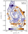 |
Fig. G.1. Distribution of α12CO(1−0) across M51 Solution pixels of M51 color-coded by their respective α12CO(1−0) value. Contours are drawn at S/N = 7, 10, 30, 50, 100 and help visualize the extent and structure of the galaxy. |
All Tables
Mean values and Kendall’s τ rank correlation coefficient (p-value given in parenthesis).
All Figures
|
Fig. 1. SDSS composite RGB image with 12CO(1–0) overlay. Color image using public SDSS data from the 16th data release (Ahumada et al. 2020). We combined the u, g, and r filter bands. Contours illustrate the IRAM 30 m 12CO(1–0) integrated intensities. The mm observations have a resolution of 23″(∼800 pc), and are indicated by the black circle in the lower left. The 10′×10′ field-of-view of our IRAM 30 m observation is indicated by the white rectangular outline. Contours are drawn at arbitrary intervals between 0.5 − 10 K km s−1 to highlight the structure of the galaxy. |
| In the text | |
|
Fig. 2. Integrated intensities. All maps have been convolved to a common beamsize of 27″ (the beamsize is indicated by the circle in the lower left corner). Color scale in units K km s−1. Contour indicates S/N = 5 of the respective CO isotopologue transition. We do not provide the C18O(1–0) emission line map since we do not detect significant emission across the galaxy. Coordinates are relative to the center coordinates in Table 1. |
| In the text | |
|
Fig. 3. Radially stacked CO spectra for rgal ≤ 4 kpc. We stack over the central 4 kpc. Furthermore, the predicted C18O(1–0) emission line is shown, based on the 13CO(1–0) emission line and assuming a line ratio of 0.2 > R18/13 > 0.1 (Jiménez-Donaire et al. 2017). The C18O(1–0) in M101 seems to be fainter than we would expect based on values from EMPIRE. The blue-shaded background indicates the line mask over which we integrate the spectrum. |
| In the text | |
|
Fig. 4. CO line ratio comparison to literature values. We compare the average R21 and R13/12 values estimated from the distribution of the M101 data points to literature values. Errorbars indicate the 1σ distribution of sample values. If the literature value corresponds to the value for a specific galaxy, the source’s name is provided. Measurement for M101 indicated by the cross. The square symbol indicates the result from M51. Left: collection of R21 distributions. Right: the R13/12 distribution is shown. Our measurement agrees well with results for M51 and the Milky Way. |
| In the text | |
|
Fig. 5. Spatial and radial variation of the CO line ratio. Top row shows the R21 line ratio while the central row shows the R13/12 line ratio. The maps (left top and middle panels) show the spatial distribution of the line ratios. The colored points show sightlines with 5σ in both integrated intensities. The 5σ contour of the 12CO(1–0) integrated intensity is shown by the solid contour. The dashed circles indicate the radial bins used for the stacking. The radial plots (right panels) show the radial trends of the line ratios. The panels in the bottom row show trends of the 12CO(2–1)/(1–0) (R21) ratio (left) and the 13CO/12CO(1–0) ratio (R13/12) (right) with the SFR surface density. The ratio derived by the stacked line brightness is indicated by the larger blue or green symbols (see Appendix C for a brief description of the stacking technique). We note that because the S/N13CO(1–0) is significantly lower than for 12CO(1–0), and more lines of sights do not show a significant detection, the stacked points yield a lower R13/12. Triangles indicate 3σ upper limits. The uncertainty of the points is indicated, but it is generally smaller than the point size. The censored region applying to the individual lines of sight is shown by the red (1σ) shaded region. The region indicates where, due to the lower average sensitivity of one observation set, we do not expect to find significantly detected data points (i.e., the region where only one dataset will be significantly detected). |
| In the text | |
|
Fig. 6. Solution pixel approach to estimate α12CO(1−0). Left: from the scatter minimization approach, described by Leroy et al. (2011) and Sandstrom et al. (2013), we obtain estimates of α12CO(1−0) and DGR. The top panels (i) show the hexagons that illustrate the individual solution pixels for both 12CO(1–0) and (2–1) transmission. The solution pixels consist of 37 underlying, half-beam spaced lines of sight. We note that the underlying hexagon tiling is meant to show the results in each solution pixel (the actual solution pixels have 40% overlap). In the maps, we highlight an individual solution pixel. We vary α12CO(1−0) and compute the DGR following Eq. (12). We select the value for which the variation in DGR is minimal. The bottom left panel (ii) shows the variation of the DGR as a function of different α12CO(1−0). The variation for the selected solution pixel is minimal for α12CO(1−0) labeled B. We perform this analysis for each solution pixel. The bottom right panel (iii) illustrates why the variance differs when changing α12CO(1−0). Here we combine all significant points from the solution pixel indicated in panel (i) from both CO lines. The black lines point to the solution pixel where the individual lines of sight are drawn from. We correct the 12CO(2–1) data with the average line ratio of the solution pixel. The panel illustrates the differences in DGR for three selected α12CO(1−0) (labeled A, B, and C). Based on the selection of α12CO(1−0) the DGR values will be positively or negatively correlated (as illustrated by the colored line, which is drawn schematically to guide the eye). Right: the resulting α12CO(1−0) value for each solution pixel based on the combined 12CO(1–0) and 12CO(2–1) integrated intensities. |
| In the text | |
|
Fig. 7. Radial α12CO(1−0) and DGR trend in M101. The left panel shows radial α12CO(1−0) trend, and the right panel illustrates radial DGR dependency. Top: smaller blue (pink) points show the individual α12CO(1−0) (DGR) measurements for the various solution pixels. Larger red (yellow) points show the derived trend based on binning the data. Bottom: residual α12CO(1−0) or DGR values after subtracting the radial trend based on linearly interpolating the binned data trend (solid red /yellow line). |
| In the text | |
|
Fig. 8. 13CO derived α12CO(1 − 0)LTE We estimate the conversion factor under LTE assumptions using the 12CO(1–0) and 13CO(1–0) emission. We perform two iterations: (i) keeping the conditions fixed across the galaxy apart from the R13/12 ratio and (ii) varying the 13CO excitation temperature,Tex, the beam filling factor ratio, η12/η13, and the 13CO abundance between disk and center using a sigmoid function. Top three panels: variation of input parameters for α12CO(1−0) derivation. Bottom Panel: radial Trend in |
| In the text | |
|
Fig. 9. DGR and α12CO(1−0) trends and atomic/molecular gas profiles Left: the trend of α12CO(1−0) and DGR as a function of the log(WCO/ΣH I), which roughly translates to the molecular-to-atomic gas fraction. The points indicate the individual solution pixels. The color indicates the galactocentric radius. The black line indicates the binned trend, and the dark-shaded region shows the 1σ scatter. The vertical dashed line is arbitrarily drawn and shows approximately beyond where the two parameters start to deviate from a flat trend. Right: radial profiles of ΣH I and Σmol at solution pixel scale resolution (∼2 kpc). The line indicates the radially binned values. The bottom panel shows the ratio of molecular to atomic gas mass surface density. The horizontal dotted line indicates unity between the molecular and atomic gas surface density. |
| In the text | |
|
Fig. 10. Comparing α12CO(1−0) trends in M101 and M51. Comparison of radial α12CO(1−0) trend in M101(red) and M51(blue). Each panel shows the trend line for both galaxies separately. The trend is determined by binning the α12CO(1−0) values of the individual line of sights. The two dashed lines show the 16th and 84th percentile distribution of the combined M51 and M101 α12CO(1−0) dataset. The shaded region around the trend line shows the respective 1σ scatter of the respective trend line fit. Left: the trend of α12CO(1−0) with galactocentric radius normalized by r25. Center: 12CO line ratio R21 correlation. The thick-dashed line shows a linear regression to the stacked data points (combining M51 and M101). The grey-shaded region between the dotted curves indicates the 1σ confidence interval of the fit. Right: trend with the 13CO-to-12CO line ratio, R13/12. The linear regression only fits the trend for M51 since no clear trend is seen for M101. |
| In the text | |
|
Fig. 11. Arm-interarm variation of α12CO(1−0)in M51. The graph shows the 12CO(1–0) intensity binned by spiral phase. The blue points show the stacked line ratio by spiral phases in steps of 20°, increasing counter-clockwise. The vertical red and blue shaded regions show the extent of spiral phases that correspond to the northern (red) and southern (blue) spiral arm of the galaxy. |
| In the text | |
|
Fig. 12. Effect of 13CO optical depth on CO line ratios under LTE (top) and non-LTE (bottom) conditions. We assume optically thick 12CO and optically thin C18O emission. Top left: variation of R18/13 with τ13CO for different abundance ratios of the 13CO and C18O species. We do not significantly detect C18O in the center of the galaxy. The orange shaded region hence shows the region where the line ratio in M101’s central 4 kpc region could fall. Average MW value (solid line; Wouterloot et al. 2008), starburst (dashed line; e.g., Tan et al. 2011), and ULIRGs (dotted; e.g., Greve et al. 2009) is shown. Top right: variation of R13/12 with τ13CO for different beam filling factor ratios between the 12CO and 13CO emission, η12 and η13. The blue band shows the range of measured R13/12 values in M101. Average MW value from Roman-Duval et al. (2016), starburst and ULIRGs from Sliwa & Downes 2017. Bottom panels: we use the line ratio model calculation provided in Leroy et al. (2022). These are based on model calculations with RADEX (van der Tak et al. 2007) and used a lognormal density distributions described in Leroy et al. (2017b). Bottom left: we fix the ratio at R21 = 0.6 and use a lognormal density distribution width of σ = 0.6. The color-coded lines show as a function of H2 volume density (x-axis) and kinetic temperature Tkin (y-axis) the trends for different total CO column densities per line width (NCO/Δν), which roughly correlate with the optical depth. Bottom center: the line ratio R21 as a function of kinetic temperature for different mean molecular gas densities. Bottom right: the line ratio R21 as a function of the mean molecular gas density for different kinetic temperatures. The green shaded region shows the 16th to 84th percentile range for the values found in M101. For the computation of R21 as function of temperature and density, we fix σ = 0.6 dex and NCO/Δv = 1016 cm−2 (km s−1)−1. We note that we assume a common excitation (density, temperature) for all species and LTE for the top panels. |
| In the text | |
|
Fig. 13. Impact of varying R21 and α12CO(1−0) on the Kennicutt-Schmidt relation We compare the KS relation using three different ways of estimating the molecular gas mass, Σmol: (i) 12CO(1–0) and a radially interpolated α12CO(1−0) derived for each galaxy (ii) 12CO(1–0) and a fixed α12CO(1 − 0)MW = 4.3 M⊙ pc−2/(K km s−1), and (iii) 12CO(2–1) and a fixed R21 = 0.6 (and R21 = 0.9 in M51; den Brok et al. 2022). The resulting KS index, N, is determined using an orthogonal distance regression (fit indicated by solid line) and indicated in each panel with its 1σ uncertainty. In addition, each panel also lists the ΣSFR value (in log) at Σmol = 10 M⊙ pc−2, as derived from the linear fit. The KS coefficient, N, the Pearson’s correlation coefficient, p, and as the SFR surface density at a molecular gas mass surface density of 10 M⊙ pc−2 or the linear relationship are indicated in each panel as well. The grey shaded region shows the ±0.30 dex dispersion which is expected for a larger sample of galaxies (Bigiel et al. 2008; Leroy et al. 2013). The points, which represent the individual solution pixels, are color-coded by their difference (in dex) in Σmol to the molecular gas mass determined using method (iii), which is shown in the right panel. Squares indicate the central points (r ≤ 2 kpc). |
| In the text | |
|
Fig. 14. Impact of varying R21 and α12CO(1−0) on the molecular gas depletion time The top panels show the radial trend of the depletion time for M101 (left), M51 (center), and for the combination of the sightlines from both galaxies (right). The depletion time depends on a measurement of the molecular gas mass. The grey points (with purple edge color) show the measurements using CO(2–1) and fixed R21 and α12CO(1−0) values. The points color-coded by SFR surface density are from using CO(1–0) and a radially interpolated α12CO(1−0). The bottom panels compare the radially binned trends of both measurements. The grey line indicates the residual between the two trend lines. |
| In the text | |
|
Fig. 15. CO(1–0)-to-H2 conversion factor prescription comparison Comparing the radial α12CO(1−0) trend derived from binning the data (in color) and the trend derived from applying different prescriptions. The trend for M101 is shown in the left and for M51 on the right. Comparison of the derived trend when applying the α12CO(1−0) prescription used Sun et al. (2022; dotted line), from Bolatto et al. (2013; dash-dotted line). The black horizontal line illustrates the average local solar neighborhood α12CO(1−0) value. The green-shaded region is an approximate illustration of the central region of the galaxy, where conditions potentially change dramatically to the overall disk. |
| In the text | |
|
Fig. A.1. H I SHORT SPACING CORRECTION The THINGS H I data cube for M101 is seriously affected by filtering and bowling artifacts. The red spectrum illustrates the spectrum for an arbitrarily selected line of sight at 650′ spatial resolution (angular resolution of the Effelsberg single-dish data). The black spectrum shows the same sightline spectrum obtained from the Effelsberg single-dish data (EBHIS survey). We used the uvcombine package to determine a single-dish scale factor of 1.7. The blue spectrum shows the resulting feathered observation for the selected sightline. |
| In the text | |
|
Fig. C.1. Radially stacked 12CO(1–0) (orange) and 13CO(1–0) (purple) spectra. For a better comparison, we scale the 13CO(1–0) brightness temperature up by a factor 5. The S/N of the 13CO(1–0) is indicated in each panel (green indicates spectra where S/N13 > 5. We stack in radial bins of size 1.25 kpc. The shaded region indicates the spectral range over which we integrate the spectra. We detect significant 13CO(1–0) emission out to rgal ∼ 8 kpc. |
| In the text | |
|
Fig. C.2. Stacked CO spectra over the full galaxy (Left) Stacked spectra over the 12CO(1–0) 3σ mask. 13CO(1–0) spectrum scaled up by a factor of 5, C18O(1–0) by a factor of 10. We mark the number of sightlines per mask with n. (Middle) Similar to the left panel, but stacked over the 13CO(1–0) 3σ mask. We do not detected significant C18O(1–0) emission. (Right) moment 0 map of 12CO(1–0). The S/N = 3 contour of 12CO(1–0) is illustrated by the solid line, while for 13CO(1–0) it is indicated by the dashed line. |
| In the text | |
|
Fig. D.1. Azimuthal Variation of R21 in M101. (Left) The 12CO(1–0) integrated intensity map with the logarithmic spirals with a pitch angle of θ = 23° overlayed. The spirals increment with a spiral phase Δψ = 20° and increment in the counterclockwise direction. The spiral bins have a with of 40°. The thick cyan line indicates ψ = 0. The four spiral arms are accordingly labeled and colored in red. For the spiral binning, we exclude the central 80′ (in diameter), belonging to the central region of the galaxy (indicated by the golden-hatched region in the middle). (Center) The map shows the R21 variation across the galaxy. Spiral bins follow the description on the left panel. (Right) The line ratio is binned by the spiral phase. The gray-shaded region shows the 1σ scatter per bin. The red-shaded region indicates the spiral phases of a particular spiral arm. |
| In the text | |
|
Fig. E.1. Comparing the Impact of Different Datasets on α12CO(1−0) Estimates. We compare the results after substituting feathered H I (left column) and non-feathered H I (right column) observations as well as different 12CO(2–1) observations (data from this project and HERACLES). The points show the resulting α12CO(1−0) value for the different solution pixels. The black line indicates the binned trend, and the shaded region illustrates the 1σ scatter per bin. The right panel shows the average values of the different permutations (color-coded). The grey point is based on using the 12CO(2–1) data only (and deriving the 12CO(1–0) data using a fixed R21). This approach reproduced the method by Sandstrom et al. (2013). The solid line indicates the average MW α12CO(1−0) value, and the dashed line shows the average value found by Sandstrom et al. (2013) for M101. |
| In the text | |
|
Fig. F.1. MC Simulation for Central Solution Pixel. The red contours show the 10%, 50%, and 75% inclusion of the solution distribution for the scatter minimization technique. Blue shows the result distribution based on the least-square minimization (Eq. ). The red and blue points show the solution before adding noise to the input parameters. |
| In the text | |
|
Fig. G.1. Distribution of α12CO(1−0) across M51 Solution pixels of M51 color-coded by their respective α12CO(1−0) value. Contours are drawn at S/N = 7, 10, 30, 50, 100 and help visualize the extent and structure of the galaxy. |
| In the text | |
Current usage metrics show cumulative count of Article Views (full-text article views including HTML views, PDF and ePub downloads, according to the available data) and Abstracts Views on Vision4Press platform.
Data correspond to usage on the plateform after 2015. The current usage metrics is available 48-96 hours after online publication and is updated daily on week days.
Initial download of the metrics may take a while.