| Issue |
A&A
Volume 643, November 2020
|
|
|---|---|---|
| Article Number | A139 | |
| Number of page(s) | 34 | |
| Section | Extragalactic astronomy | |
| DOI | https://doi.org/10.1051/0004-6361/202038328 | |
| Published online | 17 November 2020 | |
MUSE view of Arp220: Kpc-scale multi-phase outflow and evidence for positive feedback
1
Centro de Astrobiología (CAB, CSIC–INTA), Departamento de Astrofísica, Cra. de Ajalvir Km. 4, 28850 Torrejón de Ardoz, Madrid, Spain
e-mail: This email address is being protected from spambots. You need JavaScript enabled to view it.
2
INAF – Osservatorio Astrofisico di Arcetri, Largo Enrico Fermi 5, 50125 Firenze, Italy
3
Centro de Astrobiología (CSIC-INTA), ESAC Campus, 28692 Villanueva de la Cañada, Madrid, Spain
4
University of Cambridge, Cavendish Laboratory, Cambridge CB3 0HE, UK
5
University of Cambridge, Kavli Institute for Cosmology, Cambridge CB3 0HE, UK
6
IAA – Instituto de Astrofísica de Andalucía (CSIC), Apdo. 3004, 18008 Granada, Spain
7
Centro de Estudios de Física del Cosmos de Aragón (CEFCA), Plaza de San Juan, 1, 44001 Teruel, Spain
Received:
3
May
2020
Accepted:
4
September
2020
Abstract
Context. Arp220 is the nearest and prototypical ultra-luminous infrared galaxy; it shows evidence of pc-scale molecular outflows in its nuclear regions and strongly perturbed ionised gas kinematics on kpc scales. It is therefore an ideal system for investigating outflow mechanisms and feedback phenomena in detail.
Aims. We investigate the feedback effects on the Arp220 interstellar medium (ISM), deriving a detailed picture of the atomic gas in terms of physical and kinematic properties, with a spatial resolution that had never before been obtained (0.56″, i.e. ∼210 pc).
Methods. We use optical integral-field spectroscopic observations from VLT/MUSE-AO to obtain spatially resolved stellar and gas kinematics, for both ionised ([N II]λ6583) and neutral (Na IDλλ5891, 96) components; we also derive dust attenuation, electron density, ionisation conditions, and hydrogen column density maps to characterise the ISM properties.
Results. Arp220 kinematics reveal the presence of a disturbed kpc-scale disc in the innermost nuclear regions as well as highly perturbed multi-phase (neutral and ionised) gas along the minor axis of the disc, which we interpret as a galactic-scale outflow emerging from the Arp220 eastern nucleus. This outflow involves velocities up to ∼1000 km s−1 at galactocentric distances of ≈5 kpc; it has a mass rate of ∼50 M⊙ yr−1 and kinetic and momentum power of ∼1043 erg s−1 and ∼1035 dyne, respectively. The inferred energetics do not allow us to distinguish the origin of the outflows, namely whether they are active galactic nucleus- or starburst-driven. We also present evidence for enhanced star formation at the edges of – and within – the outflow, with a star-formation rate SFR ∼ 5 M⊙ yr−1 (i.e. ∼2% of the total SFR).
Conclusions. Our findings suggest the presence of powerful winds in Arp220: They might be capable of heating or removing large amounts of gas from the host (“negative feedback”) but could also be responsible for triggering star formation (“positive feedback”).
Key words: galaxies: active / galaxies: starburst / galaxies: individual: Arp 220 / galaxies: ISM
© ESO 2020
1. Introduction
The formation and evolution of galaxies are closely coupled with the growth of the supermassive black holes (BHs) at their centre (e.g. Kormendy & Ho 2013). To explain this coupling, it has been proposed that both the stellar population and the central BH of a galaxy grow and evolve by the merging of smaller gas-rich systems (Sanders et al. 1988; Di Matteo et al. 2005; Hopkins et al. 2008). In this scenario, ultra-luminous infrared galaxies (ULIRGs, L8 − 1000 μm > 1012 L⊙) appear during the final coalescence of the galaxies, when massive inflows of cool material trigger intense starbursts (SBs) in the nuclear regions, while the BH may be buried by dust and gas, which feed the BH at high rates, causing the birth of an obscured active galactic nucleus (AGN).
Powerful outflows are routinely invoked to explain the tight BH-galaxy scaling relations. These phenomena are expected to affect the physical and dynamical conditions of the interstellar medium (ISM) and thus regulate via a feedback mechanism the formation of new stars and the accretion onto the BH (e.g. Somerville & Davé 2015). Outflows are thought to have originated either from BH accretion disc winds (AGN-driven outflows; e.g. King & Pounds 2015) during vigorous growth phases of the BH (i.e. at high AGN luminosities and Eddington ratios; e.g. Fiore et al. 2017; Perna et al. 2017a; Villar et al. 2020) or from stellar winds and supernova (SN) explosions (SB-driven outflows; e.g. Hopkins 2012; but see also e.g. Naab & Ostriker 2017; Vogelsberger et al. 2020). Consequently, outflows might play a crucial role in the evolution of galaxies, especially at high redshifts (z > 1), where episodes of intense star formation (SF) and strong AGN activity were very common (e.g. Brusa et al. 2015; Talia et al. 2017; Föerster-Schreiber et al. 2018; Kakkad et al. 2020).
Local ULIRGs, which are powered by strong SBs (Genzel et al. 1998) and/or AGN (Nardini et al. 2010), present some properties similar to those of high-z luminous and dusty star-forming galaxies (e.g. Arribas et al. 2012; Hung et al. 2014; but see also e.g. Tacconi et al. 2018), allowing, therefore, the opportunity to investigate the properties of outflows and their feedback effects at the relevant scales (i.e. < kpc). In the past, several studies have demonstrated the presence of multi-phase (ionised, neutral, and molecular) gas outflows in ULIRGs (e.g. Westmoquette et al. 2012; Bellocchi et al. 2013; Veilleux et al. 2013; Arribas et al. 2014; Cicone et al. 2014; Cazzoli et al. 2016; Fluetsch et al. 2019, 2020). Most of these works, however, have focused on the study of a specific gas phase and, more critically, have resolutions (> kpc) that are unable to trace the outflow structure in detail. High-resolution and multi-wavelength observations are therefore required to study outflows in detail (e.g. Emonts et al. 2017; Pereira-Santaella et al. 2018; Cicone et al. 2020).
We have recently started a project aimed at studying, at sub-kpc scales, the 2D multi-phase outflow structure in a representative volume-limited (z < 0.165) sample of 24 local ULIRGs by combining the capabilities offered by ALMA; this is required to trace the molecular gas and VLT/MUSE-AO needed to trace the atomic neutral and ionised gas. The selection criteria, the main properties of the sample, and the path chosen to analyse and investigate multi-phase outflows will be discussed in a forthcoming paper. In this paper, we present MUSE observations of the archetypal target Arp220, whose nuclear molecular outflow has already been studied with ALMA at ∼0.1″ resolution (Barcos-Muñoz et al. 2018; Wheller et al. 2020). This manuscript is organised as follows. In Sect. 2 we present the ancillary target data. Section 3 presents the MUSE observations and data reduction. Section 4 presents the spectral fitting analysis. Section 5 reports the spatially resolved kinematics of the atomic gas. In Sect. 6 we study the ionisation mechanisms for the emitting gas; Sects. 7–9 present the main ISM properties derived from standard optical line diagnostics. In Sects. 10 and 11 we characterise the kpc-scale outflow identified in the MUSE field and its effects on the ISM. Finally, Sect. 12 summarises our conclusions. Throughout this paper, we adopt the cosmological parameters H0 = 70 km s−1 Mpc−1, Ωm = 0.3, and ΩΛ = 0.7 as well as a Salpeter initial mass function.
2. Arp220 properties
Arp220 is the nearest ULIRG (DL ≈ 77 Mpc) and is thus an ideal laboratory for studying the processes taking place in SB galaxies. It is a late-stage merger with a peculiar morphology and a heavily obscured central region (Fig. 1). Near-infrared (near-IR) and radio observations have revealed two bright sources about 1″ (370 pc) apart, thought to be the nuclei of the merging galaxies (e.g. Scoville et al. 1997). Molecular gas emission has revealed the presence of two discs around the nuclei, with radii of ≲100 pc (e.g. Scoville et al. 1997; Barcos-Muñoz et al. 2015), and an outer disc likely formed from the gas of the progenitor galaxies, with a radius of ∼1 kpc (e.g. Scoville et al. 1997; Sakamoto et al. 1999). The spin axis of the eastern (E) nucleus is aligned with that of the kpc-scale disc, while the western (W) nucleus rotates in the opposite direction. These observations suggest that Arp220 is the product of a prograde-retrograde merger of two gas-rich spiral galaxies (Scoville et al. 1997; see also Hibbard et al. 2000).
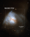 |
Fig. 1. Three-colour optical image of Arp220 obtained by combining HST observations performed through three different filters (B, B+I, and I). The white box indicates the region analysed in this work, corresponding to the MUSE FOV. North is up. Credit: NASA, ESA, the Hubble Heritage Team (STScI/AURA)-ESA/Hubble Collaboration, and A. Evans (University of Virginia, Charlottesville/NRAO/Stony Brook University). |
Arp220 experiences a powerful SB at each of the nuclei, which results in the IR prominence (LIR ∼ 5.6 × 1045 erg s−1; Nardini et al. 2010) as well as multiple radio SNe and SN remnants at each of the nuclei (Lonsdale et al. 2006; Varenius et al. 2019). There is still no convincing direct evidence, from radio to hard X-ray wavelengths, for AGN in Arp 220 (e.g. Sakamoto et al. 2008; Scoville et al. 2015; Aalto et al. 2015; Teng et al. 2015; Paggi et al. 2017). However, indirect arguments suggest that an active nucleus produces a significant fraction of the radiated power in the W nucleus (Wilson et al. 2014; Rangwala et al. 2015). Additional evidence for the presence of an AGN in the latter nucleus has recently been provided by the Fermi detection of high-energy γ-rays (Yoast-Hull et al. 2017). If an AGN is present in Arp220, it is highly Compton-thick (CT; see e.g. Teng et al. 2015). X-ray and IR data have been used to evaluate the AGN luminosity in Arp220: from the 2−10 keV emitted luminosity, Paggi et al. (2017) estimated (lower limit) AGN bolometric luminosities ∼8.3 × 1043 erg s−1 (E nucleus) and ∼2.5 × 1043 erg s−1 (W nucleus), representing only ∼1% of the bolometric luminosity (Lbol ∼ 6 × 1045 erg s−1, Sanders et al. 1988); from 5 − 8 μm spectral analysis of Spitzer data, Nardini et al. (2010) estimated an AGN luminosity of the order of ∼17% of Lbol. Veilleux et al. (2009) quantified the AGN contribution to Lbol using six independent methods based on 5 − 35 μm Spitzer data, obtaining a range of values from 0% to < 37% and an average contribution of ∼18.5% of Lbol. These results confirm that, overall, the emission of Arp220 is likely dominated by the SB component.
Whatever the energy source, Arp220 is of considerable astrophysical significance. It is a recent example of a short-lived burst of assembly and nuclear activity, which are common at z > 1 and can be used to shed light on the main physical processes governing the baryon cycle, from the fuelling of nuclear SBs and AGN with dust and gas to the feedback mechanisms that return part of this material into the circum-galactic environment. Evidence of molecular outflows in Arp220 have been inferred from the analysis of the integrated spectra of both nuclei (e.g. Barcos-Muñoz et al. 2018 and references therein). In particular, Barcos-Muñoz et al. (2018) reported the first spatially (∼0.1″) and spectrally resolved image of the molecular outflow in the W nucleus, using ALMA observations of the HCN (1–0) transition. This outflow is compact and collimated, with a bipolar morphology and an extension ≲120 pc (along the north-south direction). Recently, Wheller et al. (2020) presented new observational evidence of collimated outflows in both nuclei, using ALMA observations of carbon monoxide transition, revealing, for the first time, an outflow in the E nucleus oriented along the kinematic minor axis of the circum-nuclear molecular disc.
The ionised gas emission in Arp220 is spatially extended. XMM-Newton (Iwasawa et al. 2005) and Chandra (McDowell et al. 2003, Paggi et al. 2017) data show gas emission from several structures along the direction of the minor axis of the kpc-scale nuclear disc, on scales from 1″ (in hard X-ray) to several arcminutes (in soft X-ray; see e.g. Fig. 1 in McDowell et al. 2003). Very similar structures are observed in narrow-band Hα images (e.g. Heckman et al. 1987; Taniguchi et al. 2012). This ionised gas is more extended than the region where the IR luminosity originates (Scoville et al. 1998), and the possible connection between the nuclear and kpc-scale emitting ISM has not yet been investigated in detail. Early integral-field spectroscopy (IFS) with INTEGRAL (Arribas et al. 2001; Colina et al. 2004) has shown complex kinematics in Hα and [N II]λ6583 ionised gas along the same direction as the soft X-ray. These results were interpreted as indicative of a biconical outflow that is related to a galactic wind driven by a central SB and/or AGN (see also e.g. Heckman et al. 1990; Lockhart et al. 2015).
However, these early IFS observations were designed to map the Arp220 large-scale structures (with pixel scales > 1″), making it difficult to explain the kinematics observed in the different sub-structures that are co-spatial with X-ray emission. Moreover, these IFS data suffer from heavy obscuration by dust, preventing the detection of [O III]λ5007 and Hβ in most of the regions and, hence, the use of standard diagnostics to characterise the physical conditions of the ISM. The MUSE IFS observations presented in this paper overcome these limitations.
3. MUSE observations and data reduction
Arp220 observations were conducted as part of our programme “Sub-kpc multi-phase gas structure of massive outflows in ultra-luminous infrared galaxies” (ESO projects 0103.B-0391(A) and 0104.B-0151(A), PI: Arribas). The observations presented in this paper were carried out with MUSE in ESO Period 103, with its Adaptive Optics Wide Field Mode (AO-WFM; Bacon et al. 2010). MUSE covers a 60″ × 60″ field of view (FOV) with a sampling of 0.2″ × 0.2″, resulting in a massive dataset of ∼90 000 individual spectra. We used the nominal instrument setup, with a spectral coverage from 4750 to 9350 Å and a mean resolution of 2.65 Å (full width at half maximum; FWHM). Because of the use of adaptive optics (AO) with a sodium laser guide system, the wavelength range from ≈5800 to 5970 Å is blocked to avoid contamination and saturation of the detector by sodium light.
The requested observations were distributed in three 40 min observing blocks (OBs) with a total integration time of 2 h on source. We split the exposures in each OB into four (dithered and 90°-rotated) frames of 585 s each; because Arp220 fills most of the FOV, we also observed a black sky field for 29 s. Observations were performed with a clear sky transparency and a seeing ≈1″; the root mean square (rms) of the flux variation was ≈1%, as measured at night by the VLT DIMM station. Unfortunately, only one OB was observed, for a total observing time of 40 min on source.
Arp220 observations were reduced using the MUSE EsoReflex pipeline recipes (muse – 2.6.2), which provide a fully calibrated and combined MUSE data cube. In the last step of our data reduction, we identified and subtracted the residual sky contamination in the final data cube using the Zurich Atmosphere Purge (ZAP) software package (Soto et al. 2016). The residual contamination, due to the time difference between the sky and target acquisitions, was derived from the outermost regions of the MUSE object cube, where the sky is dominant, after masking Arp220 emission as well as background sources in the FOV.
3.1. Arp220 continuum emission and background galaxies
Figure 2 shows an image of the Arp220 continuum emission, obtained by collapsing the MUSE data cube in the wavelength range 8025 − 8125 Å (rest frame). This range is not affected by strong ISM emission lines or stellar absorption features and is free of sky lines; moreover, it is less affected by dust absorption with respect to shorter wavelengths and can provide a good tracer for the continuum emission in Arp220. A few compact sources can be identified within this MUSE narrow-band image (insets in Fig. 2, bottom left). Most of them are resolved and are associated with strong optical emission (e.g. Hα, [N II]) and absorption (e.g. Na IDλλ5891, 96) lines at the same redshift of Arp220; others are associated with background galaxies. In Table 1 we report the coordinates of these sources and the spectroscopic redshifts derived in this work (see Appendix A).
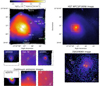 |
Fig. 2. Upper left: continuum emission from MUSE data cube, having collapsed the data cube in the range 8025 − 8125 Å (rest frame). A few bright Arp220 clumps (c1 and c2) and background galaxies are labelled (see Appendix A and Table 1); these knots are used to perform a bona fide astrometric registration of the MUSE data (see Sect. 3.2). Upper right: HST/WFC3 F160W image from HST archive (total exposure time of 172 s and pixel scale of 0.13″; PI: Larson). The image shows the region analysed in this work; the white box indicates the portion displayed in the bottom-right panel. Bottom left: zoomed-in insets of 7″ × 7″ showing the continuum emission map around some of the sources selected in the upper-left panel. The overlaid cyan contours represent the NIR emission from the HST image. For the sources in the DECaLS DR7 catalogue (Dey et al. 2018), we mark the DECaLS positions with black crosses. Bottom right: [S III]λ9069 image obtained integrating the flux in the wavelength range 9065 − 9083 Å, after subtracting the continuum emission, with overlaid contours of the NIR emission (upper-right panel). Crosses mark the [S III] nuclear peaks; white circles mark the position of two SCs identified in this work (see Sect. 6). North is up. |
Sources in the MUSE FOV towards Arp220.
3.2. Astrometric registration and angular resolution
Since no bright point sources are present in the FOV, we cannot estimate a proper spatial resolution or obtain an astrometric registration with foreground stars. We took advantage of an available near-IR Hubble Space Telescope (HST) image (Fig. 2, right) to match the position of the individual sources in the FOV (Fig. 2, bottom-left insets). We also derived a MUSE equivalent narrow-band image for the [S III]λ9069 emission line, after subtracting the continuum emission using the adjacent regions at shorter and longer wavelengths with respect to the sulphur line systemic. The regions with bright [S III]λ9069 emission perfectly resemble the near-IR HST flux distribution in the nuclear regions of Arp220 (Fig. 2, bottom-right inset). We therefore obtained a bona fide astrometric registration matching all the sources reported in the insets of Fig. 1 with those in the HST image1. We verified our astrometry by comparing the new coordinates of the background galaxies with those in the DECaLS Survey DR7 catalogue (Dey et al. 2018; black crosses in Fig. 2, bottom-left insets), obtaining a good match.
The spatial resolution of MUSE data can be roughly estimated from the [S III]λ9069 emission peaks in the bottom-right panel of Fig. 2 and the (apparent) point source galaxy at z ∼ 0.56 (Fig. A.2). The two brightest peaks in the [S III]λ9069 map (crosses in Fig. 2, bottom-right panel) can be reasonably associated with the position of the two nuclei of Arp220, since they perfectly match the near-IR emission, which, in turn, matches the location of strong X-ray emission (e.g. Lockhart et al. 2015; see also e.g. Paggi et al. 2017). We stress here that [S III]λ9069 emission provides the only diagnostic in the MUSE data cube to locate the two nuclei: In fact, all emission lines detected at shorter wavelengths and the continuum emission are strongly absorbed by dust. The two additional compact clumps with strong [S III] emission in Fig. 2 present instead properties attributable to SF, according to their optical line ratio diagnostics and kinematics (Sects. 6 and 11); they are therefore labelled as star-forming clumps (SCs hereinafter) in this work.
For each (apparent) point source in the MUSE FOV, we performed a 2D Gaussian fit and derived an estimate for the angular resolution from the FWHM of the Gaussian fit. We obtained a resolution of ∼0.56″, corresponding to ∼0.21 kpc at the distance of Arp220.
4. Spectral fitting analysis
4.1. Stellar component modelling
Prior to modelling the Arp220 ISM features, we used the penalised pixel fitting routines (pPXF; Cappellari & Emsellem 2004; Cappellari 2017) to extract the stellar kinematics. The entire wavelength range covered with MUSE (i.e. 4640−9100 Å, rest frame) was used in our analysis to model the continuum emission and recover the stellar kinematics from stellar absorption lines, after masking all optical emission lines detected in the MUSE data cube (see e.g. Fig. 4). In addition, we masked the resonant Na ID transitions, as both stellar and interstellar absorption can be at the origin of these lines. Finally, we excluded from this analysis a narrow wavelength region at ≈7630 Å (observer frame; see e.g. Fig. 4), which is associated with strong sky-subtraction residuals, as well as the region 5800−5970 Å, which is blocked by a filter to avoid contamination from the lasers (see Sect. 3).
We used the Indo-US Coudé Feed Spectral Library (Valdes et al. 2004) as stellar spectral templates to model the stellar continuum emission and absorption line systems. The models, with a spectral resolution of 1.35 Å, were broadened to the (wavelength-dependent) spectral resolution of the MUSE data (∼2.6 − 2.9 Å) before the fitting process (see e.g. Husser et al. 2016). The pPXF fit was performed on binned spaxels using a Voronoi tessellation (Cappellari & Copin 2003) to achieve a minimum signal-to-noise S/N > 16 per wavelength channel on the continuum in the [5250, 5450] Årest-frame wavelength range.
uring the fitting procedure, we used fourth-order multiplicative Legendre polynomials to match the overall spectral shape of the data. These polynomials are generally used instead of an extinction law, which was found to produce worse fits to the stellar continuum, and allow us to correct for small inaccuracies in the flux calibration (e.g. Belfiore et al. 2019).
4.2. Stellar line-of-sight velocity distributions
Figure 3 shows the Arp220 stellar kinematic maps (for a better visual output, all the maps presented from now on are centred on RA: 15:34:57.28, Dec: +23:30:11.87, corresponding to the intermediate position between the two nuclei). The systemic redshift of Arp220, z = 0.0181 ± 0.0001, has been chosen to obtain a symmetric stellar velocity gradient in the Arp220 central regions; it corresponds to the one at the position of the W nucleus (the error has been obtained by translating the positional error into velocity uncertainty).
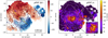 |
Fig. 3. Arp220 stellar kinematic maps from our pPXF analysis. The contours in the left-hand panel show the negative (dark blue) and positive (dark red) isovelocity curves, from −100 to +100 km s−1, equally spaced in steps of 20 km s−1; the contours in the right-hand panel are derived from the continuum emission image shown in Fig. 2 (top left) and are equally spaced in steps of 0.25 dex, starting from 1.3 × 10⁻¹⁶ erg s−1 cm−2 arcsec−2. The crosses mark the two nuclei; the dashed yellow line in the left-hand panel shows PA = 48°, corresponding to the major axis of Arp220. Right-hand panel: the inset shows a zoomed-in view of the innermost nuclear regions, highlighting the ring-like shape with high σ* values (using a slightly different colour bar); the positions of the two nuclei are shown with black crosses. Stellar velocity dispersions are not corrected for the instrumental broadening. North is up. |
The stellar velocity map (left-hand panel) allows us to define a “major axis” as the position angle (PA) along which the velocity shear is the maximum (e.g. Harrison et al. 2014). The “minor axis” is defined as the axis perpendicular to the major one. The Arp220 major axis lies along the north-east – south-west direction (PA ∼ 48°), with a distinct velocity gradient from ∼ − 100 km s−1 to +100 km s−1 in ∼3 kpc; the stellar velocities along the minor axis (PA ∼ 138°) are lower (in the range ∼[−40, 40] km s−1) and do not show clear velocity gradients. The V* map also shows different velocity-coherent structures in the outermost regions (r ≳ 10″), possibly associated with Arp220 tidal tails. In particular, the structure extending from the north in the south-western direction that is associated with positive velocities, and the western structure with negative velocities, could be associated with the two tidal tail structures emerging from the merger simulations by König et al. (2012).
The stellar velocity dispersion map (right-hand panel) shows the presence of high σ* (≳150 km s−1) in the innermost nuclear regions, but with an irregular distribution. In this region, we can recognise a ring-like structure with enhanced σ* (see zoomed-in inset). In order to define the reliability of this feature, we performed a Monte Carlo (MC) analysis using 50 simulations. In each simulation, the input spectrum was randomly perturbed within the 1σ flux errors2 and the pPXF fits were recalculated. To simplify the calculation and save computational time, only the innermost regions (in the zoomed-in inset of Fig. 3) were analysed with MC trials. The uncertainty of σ* was taken as the standard error of the fitted moment from the MC trials; its median value is 7 km s−1. Therefore, MC trials confirm the presence of enhanced σ* in the ring-like feature (see Appendix B). In order to quantify systematic errors in the velocity maps across the entire FOV, we also performed an independent fit with pPXF, using identical tessellation and wavelength coverage but different stellar templates. This analysis will be presented in Catalán Torrecilla et al. (in prep.) together with the derived stellar population parameters. Here we briefly mention that the best-fit stellar kinematics and continuum models obtained with the two approaches are consistent (within a few percentage points); in particular, the independent analysis confirmed the presence of the ring-like region and the high-velocity dispersions in several Voronoi bins out to ∼15″ from the two nuclei. Finally, we note that our reconstructed stellar kinematics are consistent with those presented in Falcón-Barroso et al. (2017) and de Amorin et al. (2017), obtained from CALIFA spectroscopic data (i.e. with poorer spatial information).
As reported in Harrison et al. (2014), the major axis corresponds to the kinematic major axis of a galaxy when the velocity map traces galactic rotation. The presence of kinematically disturbed regions, curved tidal tails, and the ring-like feature suggest that Arp220 has not yet reached its dynamically relaxed configuration. The two PAs associated with the major and minor axes, therefore, cannot be properly associated with the Arp220 kinematic axes. Nevertheless, they present well-defined and distinct properties in terms of stellar and gas kinematics, as is also shown in the next sections.
4.3. Extraction of pure ISM emission and absorption contribution
We used the pPXF best-fit models to subtract the stellar contribution from the original data cube and derive a pure emission and absorption ISM line data cube. More precisely, we subtracted the stellar emission from the original unbinned data cube by rescaling the fitted stellar contribution (constant within each Voronoi bin) to the original unbinned spectrum of each spaxel before subtracting it (e.g. Venturi et al. 2018). The separation between stellar and ISM contributions is especially needed to properly recover the Balmer line fluxes (e.g. Belfiore et al. 2019; Perna et al. 2017a) and measure the kinematics and physical properties of neutral gas in the ISM (e.g. Rupke et al. 2005a).
In Fig. 4 we report the spectra extracted from the 2 × 2 pixel regions associated with the W and E nuclei with the corresponding pPXF best-fit model profiles (orange curves). We also report the pure emission and absorption ISM spectra (blue curves) obtained by subtracting the best-fit stellar contribution. The two spectra are highly obscured (stellar colour excess E(B − V)* ≈ 1.0 from Catalán Torrecilla et al., in prep.) and are characterised by strong Hα, [N II], and [S II] lines with highly asymmetric and complex profiles (see zoomed-in insets). The [N II]/Hα and [S III]/[S II] line ratios suggest a high ionisation, typical of AGN (e.g. Kewley et al. 2001), and/or shocks (e.g. Díaz et al. 1985) produced by fast outflows (e.g. Mingozzi et al. 2019). The spectra also show neutral Na ID absorbing gas, with broad and blue-shifted components indicative of the presence of neutral outflows (see zoomed-in insets).
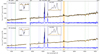 |
Fig. 4. E (top panel) and W (bottom) nucleus spectra (black curves) extracted from 2 × 2 pixel regions. The corresponding pPXF best-fit model profiles are shown with orange curves. The pure emission and absorption ISM spectra (blue curves) are obtained by subtracting the best-fit stellar contribution from the original spectra. The insets show the spectra and stellar models around Na ID and the Hα+[N II] complex. The vertical blue lines mark the wavelengths of the emission lines detected in the two spectra; the green lines mark the position of stellar absorption systems (from left to right: MgI triplet, Na ID and KI doublets, CaII triplet). The regions excluded from the pPXF fits, and corresponding to the most intense sky line residuals, are highlighted as shaded orange areas; the portion of the spectra around 5700 Å is missing because of a filter blocking the laser contamination. |
Prior to modelling the ISM features and deriving spatially resolved kinematic and physical properties of Arp220 gas, we generated Hα and [N II]λ6583 emission line images by collapsing the ISM data cube on the core of the two emission lines ([−150,+150] km s−1 in velocity space, considering the Hα and [N II]λ6583 systemics as zero-velocity). Assuming a similar kinematic behaviour for gas and stars, this emission should trace the less perturbed gas in the merging system, as the stellar component has velocities in the range ≈[−130, +130] km s−1. The two maps are reported in Fig. 5; for easier comparison with stellar kinematic maps, we show, in the left-hand panel, the stellar continuum emission (contours as in Fig. 3). Large-scale rings, arcs, and filaments, as well as diffuse line emission, can be observed across the MUSE field; several clumps are also observed, especially along PA ∼ 138° (the north-west to south-east direction). We note that MUSE observations do not cover the entire extension of the ionised gas in Arp220, with its well-known figure-eight structure that is due to bipolar lobes (e.g. Heckman et al. 1987), since the eastern arc is mostly outside the MUSE FOV (see also Fig. 1).
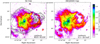 |
Fig. 5. Hα and [N II]λ6583 channel maps obtained by collapsing the ISM data cube on the emission line core (i.e. velocity channels within [−150, +150] km s−1 from the systemic). Contours in the left-hand panel are derived from the continuum emission image shown in Fig. 3, top left; contours in the right-hand panel show the 0.5 − 8 keV emission from Chandra-ACIS observations (OBSID 16092; Paggi et al. 2017). |
The Hα and [N II]λ6583 maps display similar spatial distributions, although [N II] emission appears more extended and brighter, especially along PA ∼ 138° and in the western lobe. The match between optical line and X-ray emission along PA ∼ 138° is made explicit in the right-hand panel of Fig. 5, where we represent the broadband 0.5 − 8 keV emission from Chandra-ACIS with black contours (Paggi et al. 2017).
4.4. Ionised gas feature modelling
The emission line profiles in Arp220 are highly complex, likely because of the superposition of several kinematic components associated with tidal tails (e.g. König et al. 2012), compact SCs (e.g. Wilson et al. 2006; Varenius et al. 2019), diffuse emission, and (probably) inflows and outflows (Arribas et al. 2001; Colina et al. 2004). The Hα and [N II] lines, the brightest features in the Arp220 optical spectra, generally show double peaks and prominent blue and/or red wings.
As a first step, we fitted single Gaussians to the relevant emission line tracers of the gas. In particular, we modelled the Hβ and Hα lines, the [O III]λλ4959,5007, [N II]λλ6548,83, and [S II]λλ6716,31 doublets, and the [O I] emission lines at 6300 and 6364 Å. We constrained the wavelength separation between emission lines in accordance with atomic physics; moreover, we fixed the FWHM to be the same for all the emission lines. Finally, the relative flux of the two [N II] and [O III] components was fixed to 2.99, the relative flux of the two [O I] lines was fixed to 3.13, and the [S II] flux ratio was required to be within the range 0.44 < f(λ6716)/f(λ6731) < 1.42 (Osterbrock & Ferland 2006).
Before proceeding with the fit, we derived a second Voronoi tessellation to achieve a minimum S/N = 7 of the [O III]λ5007 line for each bin. This feature is generally very faint across the FOV because of the significant dust reddening. The Hβ is even fainter and is undetected in several regions, even after this tessellation. However, we chose to use the [O III] line as a reference for the tessellation to limit the loss of important spatial information (both for kinematics and emission line structures). This, of course, will restrict our knowledge regarding the ISM physical conditions (e.g. dust attenuation and ionisation conditions) that are generally derived through emission line ratios involving the Hβ flux.
All emission lines were fitted simultaneously with our own suite of python scripts, and using the Levenberg–Markwardt least-squares fitting code CAP-MPFIT (Cappellari 2017). In this first step, we did not model the Na ID or [S III] lines. The former would require the use of multiple components to trace the emitting and absorbing contributions and will be analysed in later steps (Sect. 4.5). The sulphur line is only detected in the innermost nuclear part (see Fig. 2). This feature, generally used to constrain the ionisation conditions of warm material (e.g. Kewley & Dopita 2002; Cresci et al. 2017; Mingozzi et al. 2020), will be analysed in Sect. 6.
4.4.1. Single Gaussian fit results
Figure 6 shows the best-fit results from a single component parameterisation. The left-hand panel shows the [N II]λ6583 integrated flux, which clearly resembles the main features observed in Fig. 5, though with some loss of spatial information. The central panel shows the ionised gas velocity (associated with the centroid of the Gaussian profile); a clear velocity gradient can be observed along PA ∼ 48°, as observed in the stellar velocity map (Fig. 3) and in the CO molecular gas (e.g. Figs. 5 and 6 in Scoville et al. 1997). More disturbed kinematics are found along the perpendicular direction (PA ∼ 138°). Gas and stars in the innermost nuclear regions are kinematically aligned (with a major axis ∼48°), but the gas velocity amplitude is significantly higher when compared to that of the stars.
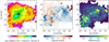 |
Fig. 6. Left: [N II] integrated flux obtained from single Gaussian fits. The first solid contour is 3 × 10⁻¹⁷ erg s−1 cm−2 arcsec−2, and the jump is 0.5 dex. Centre and right: velocity and FWHM maps obtained from single component fits. The solid contours are from the left-hand panel. The crosses mark the two nuclei. |
The right-hand panel of Fig. 6 shows the FWHM map. It further highlights the presence of highly perturbed gas along PA ∼ 138°; moderate line widths can also be observed along the bright arcs located at about 25″ west.
There are at least four regions along PA ∼ 138° with FWHM ≳ 800 km s−1. The first, at about 2″ north-west of the central position, has been associated with a bubble in Hα+[N II] of ∼1.6″ (600 pc) in diameter by Lockhart et al. (2015). They used HST/WFC3 narrow-band filters to create high spatial resolution emission line maps, but without resolving the individual contributions from Hα and [N II] (the lines are within the same WFC3 filter) or inferring kinematic information. Additional narrow-band filters centred on the Hβ and [O III] lines were used to map the [O III]/Hβ flux ratios; the bubble was associated with the highest flux ratios in the field (log [O III]/Hβ ≈ 0.2 − 0.3)3, which indicates high-ionisation conditions. They also find a clear spatial correlation with X-ray soft emission (see e.g. Fig. 5) and suggest that an AGN jet or an (AGN- or SB-driven) outflow could be responsible for the bubble. This interpretation is also consistent with the presence of high-velocity H21 − 0 S(1) line emission at the base of the bubble (with FWHM ≈ 600 km s−1), which was observed with VLT/SINFONI by Engel et al. (2011). The extreme kinematics we observe in the optical lines (Fig. 6) are fully consistent with this scenario. Moving north-west along PA ∼ 138°, we find another region with high-velocity dispersion, possibly associated with the over-position of the emission from the main system and the inner western arm. The last two areas with extreme line widths are located at ∼10″ south-east. They have a significant velocity offset with respect to the systemic of Arp220 of ≈ − 400 km s−1 (inner part) and ≈ + 300 km s−1 (outer part; see Fig. 6, centre), and are associated with intense X-ray soft emission (Fig. 5).
To summarise, these preliminary analysis results support the hypothesis of a kpc-scale (AGN- or SB-driven) outflow along PA ∼138°. A more detailed kinematical and physical analysis testing this scenario is presented in the next sections.
4.4.2. Emission line decomposition
Because of the extremely complex structure of Arp220, the spaxel-by-spaxel fit with a standard multi-component approach (e.g. Perna et al. 2019; Venturi et al. 2018) leads, in some regions, to unphysical discontinuities in the derived kinematic components and flux distributions of individual components. We therefore decided to apply a different method that allows a more appropriate regularisation of the best-fit parameters (see also e.g. Shimizu et al. 2019 for a similar approach).
A visual inspection of the spectra associated with the more disturbed kinematics in Fig. 6 revealed the presence of multiple components, which contribute to the increase in the measured velocity dispersion in the single Gaussian fits. These kinematic components could be related to either strong SF or AGN emission, tidal streams, or gas inflows and outflows, or a combination of these factors.
We started by visually selecting the 2 × 2 pixel integrated spectra showing Hα+[N II] complex with clear evidence of additional peaks and/or inflection points that, at first sight, could be related to the presence of several distinct kinematic components. A couple of these spectra are shown in Figs. 7 and 8 (top panels). Then, for each spectrum, we performed a second fit using four (at maximum) Gaussian profiles per emission line; in the following, all line profiles associated with given kinematic parameters (i.e. velocity and FWHM) will be referred to as a Gaussian set. For each set of Gaussian functions, we considered the same constraints mentioned in the previous section. The number of Gaussian sets (i.e. distinct kinematic components) used to model the spectra was derived on the basis of the Bayesian information criterion (BIC; Schwarz 1978), which uses differences in χ2 that penalise models with more free parameters (see e.g. Harrison et al. 2016; Concas et al. 2019).
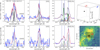 |
Fig. 7. Illustration of the profile decomposition method. Top: first three panels show the spectra in the vicinity of the [O III] (left), [O I]λ6300 (centre), and [N II]+Hα lines (right). The red curves represent the best-fit models obtained from 500 MC trials. For all but the [N II]λ6583 and Hα lines, we show the Gaussian profiles used to reproduce the spectrum with grey curves. Different colours are used for the Hα and [N II]λ6583 lines to distinguish the different kinematic components. Dashed grey and blue lines mark the Arp220 systemic and the local stellar velocity, respectively. Right-hand panel: parameter space V − FWHM–[N II]/Hα for the same kinematic components, highlighting the clear separation between the four Gaussian sets. Bottom: best-fit results for one of the nearby Voronoi bins, obtained with the kinematic constraints from the 2 × 2 spectra shown in the top panels. Bottom-right panel: velocity dispersion map with the Voronoi bins (black outlines) associated with the above-defined kinematic constraints; the black (red) contours mark the spaxels from which the top (bottom) spectra have been extracted. |
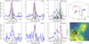 |
Fig. 8. Illustration of the profile decomposition method. See Fig. 7 for details. In this region, the velocities of the blue and green Gaussian sets overlap; a clear separation between the two is, however, assured thanks to their distinct FWHMs. |
We then used a statistical approach to study the possible degeneracy between the different Gaussian sets. We used 500 MC trials of mock spectra obtained from the best-fit models, adding Gaussian random noise4 (e.g. Perna et al. 2019) to obtain a distribution for the kinematic parameters associated with each Gaussian set (namely, the velocity V and the FWHM). The distribution in the 2D parameter space V versus FWHM is then used to check that there is no overlap between the high-probability regions of the distinct Gaussian sets, considering the 95% occurrence intervals for each kinematic parameter. In Figs. 7 and 8 (top right) we display the V − FWHM–[N II]/Hα parameter space obtained from the MC trials, showing that the decomposition can also sometimes be used to distinguish between distinct emission line ratios.
After identifying the individual kinematic components in a given 2 × 2 pixel spatial region, we fitted the adjacent Voronoi bins by performing a parameter tuning using the best-fit kinematic components from the original 2 × 2 spectrum, but leaving the velocity parameters free to vary within the ranges defined with our MC trials in the previous step (considering 95% occurrence intervals). In a few cases (i.e. when the MC trials give back tight high-probability regions), the lower and upper bounds associated with V and FWHM were opportunely refined during this step, while still avoiding an overlap between different components in the kinematic space, according to the above-mentioned criteria. A chi-square goodness of the fit test determined if the new Voronoi bin could be associated with these kinematic components.
In Figs. 7 and 8 (lower panels) we show the best fit in one of the nearby bins obtained with the kinematic constraints from the 2 × 2 spectra. These figures show that the spectra, regardless the apparent diversity in the (Hα+[N II]) line profiles, can be reproduced with similar kinematics. The lower-right panels also indicate the regions where kinematic properties can be obtained using the constraints from the initial 2 × 2 spectrum.
We note that the converged solutions (Figs. 7 and 8, top right) are not claimed to represent the actual physical components responsible for the observed line profiles. In fact, for instance, our results are still based on the assumption that emission lines can be represented by a combination of Gaussian profiles (but see e.g. Liu et al. 2013; Cresci et al. 2015a) and that the same kinematic component can be associated with both low- and high-ionisation lines (i.e. that there is no gas stratification with respect to the ionisation source, see e.g. De Robertis & Osterbrock 1986). Nevertheless, this approach allows us to avoid unphysical discontinuities in those regions that have more complex kinematic structures.
With this approach, we selected 11 spatial regions with well-determined kinematic properties (and, in a few cases, [N II]/Hα flux ratios; see Sect. 11). In Appendix C we report all the 2 × 2 pixel spectra as well as the location and the extent of the selected regions.
4.5. Neutral gas feature modelling
Taking advantage of the emission line decomposition described in the previous section, we performed a new multi-component Gaussian fit for the entire data cube, using the parameter tuning for the Voronoi bins within the 11 regions. In this new fit, we also simultaneously modelled the contribution of the HeI emission and the Na ID complex system, the latter of which traces the neutral gas component of the ISM.
Na ID is a resonant system and both absorption and emission contributions can be observed across the extension of a galaxy (e.g. Prochaska et al. 2011). The sodium emission has been observed at very low levels in stacked SDSS spectra (Chen et al. 2010; Concas et al. 2019) and in a few nearby galaxies (Rupke & Veilleux 2015 and references therein; Perna et al. 2019; Baron et al. 2020). A visual inspection of the Arp220 data cube revealed the presence of significant Na ID absorption and emission across the MUSE FOV: The absorption is stronger towards the bright continuum source; the emission is stronger in the north-western regions and on the eastern side of the FOV.
We fitted the observed profiles of the sodium lines in absorption with a model parameterised in the optical depth space (e.g. Rupke et al. 2002, 2005b), starting from the equation of radiative transfer (Spitzer 1978) in the case of a homogenous absorber of matter and a partial coverage of the background emission source. Following Sato et al. (2009), the Na ID doublet profile is modelled by
![Mathematical equation: $$ \begin{aligned} I(\lambda )&= I_{\rm em}(\lambda )\times f_{\rm ABS}(\lambda ) \nonumber \\&= I_{\rm em}(\lambda )\times (1- C_{\rm f} \times [1-\exp (-\tau _0 e^{-(\lambda - \lambda _{\rm K})^2/(\lambda _{\rm K}b/c)^2} \nonumber \\&\qquad \qquad \qquad \qquad \qquad - 2\tau _0 e^{-(\lambda - \lambda _{\rm H})^2/(\lambda _{\rm H} b/c)^2})]), \end{aligned} $$](/articles/aa/full_html/2020/11/aa38328-20/aa38328-20-eq1.gif) (1)
(1)
where H and K indicate the sodium transitions at 5891 and 5896 Å, Cf is the covering factor, τ0 is the optical depth at the line centre λK, b is the Doppler parameter (![Mathematical equation: $ b=FWHM/[2\sqrt{\ln(2)}] $](/articles/aa/full_html/2020/11/aa38328-20/aa38328-20-eq2.gif) ), and c is the light velocity. This model assumes that the velocity distribution of absorbing atoms is Maxwellian and that Cf is independent of velocity. Following Rupke et al. (2005b), we assumed the case of partially overlapping atoms on the line of sight (LOS), so that the total sodium profile can be reproduced by multiple components, and
), and c is the light velocity. This model assumes that the velocity distribution of absorbing atoms is Maxwellian and that Cf is independent of velocity. Following Rupke et al. (2005b), we assumed the case of partially overlapping atoms on the line of sight (LOS), so that the total sodium profile can be reproduced by multiple components, and  , where
  is the ith component (as given in Eq. (1)) used to model the sodium features (see also Sect. 3.1 in Rupke et al. 2002).
The term Iem(λ) in Eq. (1) represents the intrinsic (unabsorbed) intensity, defined as I* + IHeI, where I* is the best-fit model obtained from pPXF analysis and IHeI is the helium line intensity. This emission line is modelled together with the features in the [O III]+Hβ and Hα+[N II] regions using Gaussian profiles.
Atomic neutral Na ID features and ionised lines are modelled simultaneously, using up to four kinematic components. Namely, the kinematic parameters of a given Gaussian set (used to model ionised lines) also define the Na ID absorption (i.e. fABS(λ)) or emission kinematics. In the case of Na ID emission, the Na ID doublet line ratio is free to vary between the optically thick (f(H)/f(K) = 1) and thin (f(H)/f(K) = 2) limits (e.g. Rupke & Veilleux 2015). To avoid degeneracies between positive and negative contributions at the same velocities, we considered the following two conditions during the fitting procedure: (1) a given kinematic component (i.e. a Gaussian set) cannot be associated with both absorption and emission Na ID contributions; and (2) the kinematic component associated with Na ID emission line contribution is, if present, always red-shifted with respect to the absorption component(s) (e.g. Prochaska et al. 2011).
Figure 9 shows the best-fitting models for some representative spectra in the vicinity of the Na ID complex. The different panels display the range in emission and/or absorption line profile shapes detected in the MUSE FOV. Although our model considers several assumptions, it is able to describe the observed spectra well.
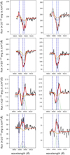 |
Fig. 9. Best-fitting models for eight representative spectra in the vicinity of the Na ID complex. The original spectra are shown in black and the pPXF best-fit models in orange; the red profiles represent the best-fit models obtained with the simultaneous multi-component approach. Green, grey, and blue profiles are obtained from Eq. (1) and represent the different kinematic components used to model the Na ID absorption; in the last four panels, the Na ID emission line contribution (modelled with Gaussian profiles) is shown with an arbitrary offset in the y-axis. |
5. Gas kinematics
In this section we briefly discuss the general results we obtained from the multi-component fits described above. The properties of the individual components will be discussed in later sections. Gas kinematics are traced taking into account two non-parametric velocities (e.g. Zakamska & Greene 2014): v50, the velocity associated with the 50% percentile, and W80, defined as the line width comprising 80% of the flux (and corresponding to 1.09 × FWHM for a Gaussian profile). For the Na ID system, all velocities are defined using the H component wavelength as a zero-point; correspondingly, v50 and W80 are computed using the best-fit H components and not the whole doublet profile5. Line features are typically non-Gaussian and broad; therefore, we do not correct line velocities for the instrumental broadening.
In Fig. 10 we report the [N II] flux, velocity, and line width maps obtained from the total line profiles (i.e. integrating over the different kinematic components required to reproduce the line profiles). These maps are similar to those in Fig. 6, which were obtained with single Gaussian fits, but the present ones are more precise (e.g. maps in Fig. 6 overestimate fluxes and widths in the more external regions). The Hα flux, velocity, and line width maps obtained from multi-component fits are very similar to those of [N II]. On the contrary, [O III] and Hβ are noisier and their distributions are fuzzy because of the lower S/N; nonetheless, these faint features reveal the same structures observed in [N II] maps (Appendix D).
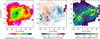 |
Fig. 10. [N II] multi-component fit results. Left: integrated flux; the first solid contour is 3 × 10⁻¹⁷ erg s−1 cm−2 arcsec−2, and the jump is 0.5 dex. Centre: [N II] velocity (v50) map. Right: [N II] line width (W80) map. The solid contours are from the left-hand panel. The crosses mark the two nuclei. |
In Figs. 11 and 12 we report the equivalent width6 (EW) and kinematic maps derived for the Na ID emission and absorption contributions. The ionised and neutral gas velocity dispersion maps are roughly consistent: They confirm the presence of highly perturbed kinematics along PA ∼ 138° and in the western and eastern lobes, with W80 up to 800 km s−1. In particular, the highest W80 associated with Na ID emission are found in the western lobe, while those associated with Na ID absorption are along PA ∼ 138°, within 10″ from the two nuclei.
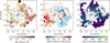 |
Fig. 11. Na ID emission line maps from the multi-component fit. Left: EW. Centre: Na ID velocity (v50) map. Right: Na ID line width (W80) map. The solid contours and crosses are from Fig. 10. |
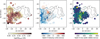 |
Fig. 12. Na ID absorption line maps from the multi-component fit. Left: EW. Centre: Na ID velocity (v50) map. Right: Na ID line width (W80) map. The solid contours and crosses are from Fig. 10. |
The [N II] and Na ID velocity maps are less consistent: The velocity gradient along PA ∼ 48°, already revealed by stars as well as ionised and molecular gas, is also detected in the absorbing Na ID gas. The cold gas absorption dominates over the Na ID emission within the innermost regions (r ≲ 10″), with an EW up to ∼10 Å; it presents strong negative velocities along PA ∼138°, similar to those of the ionised counterpart. In order to facilitate the comparison between the different emitting and absorbing components, we report, in Fig. 13, the velocities we derived from the analysis of MUSE data together with CO(2–1) measurements (from Scoville et al. 1997) along PA = 48° and PA = 138°. Overall, the two position-velocity trends confirm the presence of a velocity gradient along PA = 48° and multi-phase (i.e. neutral and ionised) approaching gas along PA = 138°. We note, however, that Na ID velocities along PA = 48° are always red-shifted with respect to the stars, especially in the innermost region (≲4″). Because of the geometrical configuration that is required to observe absorption features, this absorbing gas could, in principle, trace an inflow of neutral gas towards the innermost regions where the nuclei and associated SBs are located. However, the good agreement between the neutral and ionised gas velocities questions this interpretation, as the latter seems to follow a rotation pattern. Therefore, an alternative explanation is that the neutral and ionised gas is confined to a rotating disc, with lower velocity dispersions and higher velocity amplitudes with respect to the stars. If this is the case, the motion of stars would take place in a thicker disc, while the gas is confined to a thinner region.
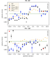 |
Fig. 13. Position-velocity diagram, with positions varying along PA = 48° (top) and PA = 138° (bottom) for the stellar component, [N II] gas, and Na ID gas, as labelled in the figure. Distances on the x-axis are measured from the intermediate position between the two nuclei, from the bottom to the top of the FOV. Stellar and gas velocity measurements are obtained by averaging 3 × 3 pixels along a given PA from the maps shown in Figs. 3, 10–12; CO(2–1) velocities are obtained from Fig. 5 in Scoville et al. (1997). |
In the more external regions, we observe a significant Na ID emission (EW ≈ 3Å), mostly associated with approaching gas on the western side and receding gas on the eastern side. In the latter region, Na ID is associated with P-Cygni profiles, with approaching absorbing gas and receding emitting material (see also Fig. 9). The presence of off-nuclear Na ID emission is consistent with the results presented for IRASF05189−2524 by Rupke & Veilleux (2015), who reported an anti-correlation between Na ID brightness and optical continuum attenuation. A more quantitative comparison between these quantities in Arp220 will be investigated in an upcoming paper (see Sect. 8).
A visual inspection of the best-fit results reveal that in the innermost nuclear part (i.e. within ∼10″ of the two nuclei), and especially along PA ∼ 138°, both approaching and receding gas emissions are detected as blue-shifted and red-shifted components (see e.g. Figs. 7 and 8; see also the velocity channel maps in Fig. 19), consistent with the presence of powerful outflows. On the other hand, the more external regions are associated with simpler profiles; in particular, the arcs in the north-western lobe are dominated by approaching gas, while the south-western arcs are mostly dominated by red-shifted emission. The high W80 observed in the latter regions could therefore be explained by the superposition of different streams and tails along the LOS (see e.g. König et al. 2012), although other mechanisms cannot be excluded.
6. Ionisation conditions
In this section we investigate the dominant ionisation mechanism(s) for the emitting gas across the MUSE FOV using standard emission line ratios (e.g. Baldwin et al. 1981; Veilleux & Osterbrock 1987; Díaz et al. 2000) and line widths (e.g. Dopita & Sutherland 1995). The close wavelengths of the line pairs involved in such diagnostics ensure minimum dust reddening effects. The only exception is the Díaz et al. (2000) diagnostic that involves [S II] and [S III] transitions, for which we applied the extinction corrections introduced in Sect. 8.
6.1. BPT diagnostics
Figure 14 (top-left panel) shows the [O III]λ5007/Hβ versus [N II]λ6584/Hα flux ratios ([N II]-BPT diagram hereinafter), derived by integrating the line flux over the entire fitted profiles, for only those Voronoi bins in which all the emission lines are detected with an S/N > 3. The points in the diagnostic diagram are colour-coded using a function of the two line ratios, defined as the emission line ratio function ELR (Eq. (1) in D’Agostino et al. 2019):
 (2)
(2)
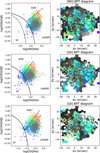 |
Fig. 14. Arp220 resolved-BPT diagrams. Left-hand panels: we report the [N II]-BPT (upper), [S II]-BPT (centre), and [O I]-BPT (bottom) diagrams for each Voronoi bin with S/N > 3 in each line. Black curves separate AGN-, SF-, and LI(N)ER-like line ratios (see text for details). For each diagnostic, a map marking each Voronoi bin with the colour corresponding to increasing flux ratios is shown on the right. The colour codes are defined using the ELR functions described in the text. Grey points correspond to [O III]/Hβ lower limits; light-to-dark grey colours in the maps correspond to increasing [N II]/Hα (top right), [S II]/Hα (middle), and [O I]/Hα (bottom) ratios. The contours of [N II] line emission are over-plotted in black. Most of the gas emission is dominated by LI(N)ER-like ionisation. In the [S II]-BPT map, we labelled the position of the four SCs identified in this work. |
with X = [N II]/Hα and Y = [O III]/Hβ. The same colours are also reported in the map of Arp220 (top-right panel) to distinguish the different ionisation sources in the FOV: purple-to-blue colours identify regions with the lowest line ratios, while green-to-orange colours identify the Voronoi bins with the highest line ratios.
The flux ratio errors are not reported in the figures. These uncertainties, as shown for instance in Fig. 8, can be significant (up to a few 0.1 dex), both because of the S/N levels and the degeneracies in the fit analysis.
The Hβ line is undetected in several Voronoi bins because of the strong dust attenuation. Therefore, we decided to include in these diagrams the (grey) points associated with [O III]/Hβ lower limits, derived using a 3σ upper limit for the flux of the (undetected) Hβ line. In the Arp220 map, the colour intensity of grey Voronoi bins (from light to dark grey) is coded as a function of increasing [N II]/Hα.
The curves drawn in the diagrams correspond to the maximum SB curve (Kewley et al. 2001) and the empirical relation (Kauffman et al. 2003a) used to separate purely SF galaxies from composite AGN-SF galaxies and AGN- and/or low-ionization (nuclear) emission-line region (LI(N)ER)-dominated systems (e.g. Kewley et al. 2006; Belfiore et al. 2016); the dot-dashed line is from Cid et al. (2010) and is used to separate LI(N)ERs and AGN. The [N II]-BPT diagram shows that the SF ionisation is found in the source at ∼30″ west of the nuclei (RA 15:34:54.7, Dec 23:29:58 in Fig. 5); composite line ratios are found in a handful of Voronoi bins, mostly associated with an SC at ∼5″ east of the nuclei. Most of the Voronoi bins have very high [N II]/Hα and relatively low [O III]/Hβ ratios, resulting in LI(N)ER-like line ratios. The highest line ratios are found in the proximity of the bubble and the high-v structures.
All [O III]/Hβ lower limits are in the LI(N)ER region as well. These estimates are consistent with the measurements derived by Lockhart et al. (2015) for the gas along PA ∼ 138° using HST narrow-band filters (with average log([O III]/Hβ) ≈ 0.1 along PA ≈ 138°).
In Fig. 14 we also report the [O III]/Hβ versus [S II]λλ6716,31/Hα flux ratios ([S II]-BPT diagram hereinafter; central panels) and the [O III]/Hβ versus [O I]λ6300/Hα flux ratios ([O I]-BPT hereinafter; bottom panels). Colour codes are derived using the ELR function (Eq. (2)), with X = [S II]/Hα for the [S II]-BPT and X = [O I]/Hα for the [O I]-BPT.
The lines drawn in the diagrams correspond to the optical classification scheme from Kewley et al. (2006, 2013) and confirm the ubiquity of LI(N)ER-like line ratios across the MUSE FOV. These two diagrams also show the presence of a second SC at ∼8″ east (SC2 in the [S II]-BPT map) and low line ratios along a stream in the western regions.
It should be kept in mind that the lines in the BPT diagrams do not provide a sharp separation between the different ionisation mechanisms. In particular, LI(N)ER-like line ratios could indicate the presence of: (i) a low-ionisation emission from AGN (e.g. Heckman 1980; Baron & Netzer 2019); (ii) SF and/or AGN activity in a high metallicity environment (see e.g. Figs. 1 and 4 in Kewley et al. 2013); or (iii) fast shocks induced by SB- and/or AGN-driven winds or galaxy interactions (e.g. Allen et al. 2008)7. In fact, the location of the separation lines between SF and AGN ionisation in the diagrams strongly depends on the metallicity regime of the ISM (e.g. Kewley et al. 2013). On the other hand, general shock models predict line ratios that can cover a very large range in the BPT diagrams (e.g. Alarie & Morisset 2019). The high [N II]/Hα, [S II]/Hα, and [O I]/Hα ratios measured in Arp220 allows us to exclude stellar photoionisation in almost every Voronoi bin, but BPTs alone do not allow us to discriminate between AGN and shock ionisation. We therefore investigated the gas conditions in more detail by considering additional diagnostics to isolate the cause(s) of the line emission.
6.2. Ionisation parameter diagnostics
Arp220 resolved-BPT diagrams could be consistent with the predictions of AGN photoionisation models with an ionisation parameter log U ≲ −3 and metallicities 12 + log(O/H) ≳ 8.7 (e.g. Groves et al. 2004; Davies et al. 2016; Baron & Netzer 2019). In order to measure the U parameter, defined as the number of ionising photons S* per hydrogen atom density nH divided by the speed of light c, we used the [S III]λλ9069, 9532/[S II]λλ6716, 31 ratio (e.g. Díaz et al. 2000). Since [S III]λ9532 is not covered by the wavelength range observed by MUSE, we adopted a theoretical ratio of [S III]λ9532/[S III]λ9069 = 2.5 (Osterbrock & Ferland 2006), fixed by atomic physics. The [S III]λ9069 line was modelled using the best-fitting kinematic parameters obtained for the optical lines (i.e. the kinematics and the number of components per individual Voronoi bin).
In Fig. 15 we show the [S III]/[S II] ratio map of Arp2208. The [S III] emission is detected only in the vicinity of the two nuclei and the clumps SC1 and SC2; on the contrary, [S II] lines are detected across most of the MUSE field. We found log([S III]/[S II]) in the range from ≈ − 0.2 (log U ≈ −3, in the nuclei and SCs) to ≈ − 1 (log U ≈ −4.5, in the circum-nuclear regions). Even lower ionisation parameters might be associated with the regions where [S III] is undetected.
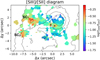 |
Fig. 15. Arp220 map of the [S III]λλ9069, 9532/[S II]λλ6716, 31 ratios, obtained from the fitted total line profiles. Emission line fluxes have been corrected for extinction (see Sect. 8). The contours of [N II] line emission and the position of the E and W nuclei are over-plotted in black. |
Unfortunately, standard metallicity diagnostics are not calibrated for LI(N)ER-like line ratios (Dopita et al. 2016; Curti et al. 2017) and cannot be used. Therefore, with the information collected so far, we cannot confirm that ISM conditions in Arp220 are consistent with the AGN ionisation expectations mentioned above.
6.3. Shock diagnostics
In order to investigate the possible contribution of shock excitation, we studied the correlation between the gas kinematics and the ionisation state. The line ratios produced in photoionised regions should be independent of the gas kinematics, but they are expected to correlate with the kinematics of the shock-ionised material (e.g. Monreal-Ibero et al. 2006; Arribas et al. 2014; McElroy et al. 2015; Perna et al. 2017b; Mingozzi et al. 2019).
In Fig. 16 (top panels) we show W80[NII] against [N II]/Hα, [S II]/Hα, and [O I]/Hα with colours from purple to red going from low to high flux ratios and line widths; in the bottom panels, we report the corresponding positions on the Arp220 map. The figure shows that the highest line ratios come from the regions with the highest W80. To explore the possible correlations between flux ratios and line widths, we report, in Fig. 16 (top panels), the predicted [N II]/Hα, [S II]/Hα, and [O I]/Hα as a function of shock velocity (Vs) from grids of shock models calculated with the code MAPPING V (Sutherland & Dopita 2017; Sutherland et al. 2018). The models were extracted from the 3MdBs database (Alarie & Morisset 2019), using the exact replica of the Allen et al. (2008) grids with magnetic field values in the range 1 − 10 μG, shock velocities in the range 200 − 1000 km s−1, and a fixed pre-shock density of 1 cm−3, and assuming metallicities of 1 Z⊙ (dashed lines) and 2 Z⊙ (solid lines). The measured W80 may depend on shock geometry and is not predicted in the shock models, although a positive correlation between Vs and W80 is expected. The predicted trends in Fig. 16 are therefore shown assuming a one-to-one correlation between the two velocities.
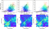 |
Fig. 16. Top panels: W80[NII] against log([N II]/)Hα, log([S II]/)Hα, and log([O I]/)Hα, from left to right, obtained from the fitted total line profiles. The plotted measurements are colour-coded from purple to red, going from low to high flux ratios and line widths. Dashed and solid lines represent shock model grids from MAPPING V (Sutherland & Dopita 2017; Sutherland et al. 2018). Each line connects predicted line ratios of a certain metallicity (1 Z⊙, solid lines; 2 Z⊙, dashed lines), pre-shock electron density (1 cm−3), and magnetic field (from 1 to 10 μG, as labelled in the first panel for 2-Z⊙ models), with changing shock velocities Vs in the range 200 − 1000 km s−1. We assumed a one-to-one correlation between Vs and W80. Bottom panels: Arp220 maps associated with the top panel diagrams, using the same colour codes. |
The [N II]/Hα and [S II]/Hα diagrams show a clear match between our measurements and the predicted trends, confirming the close connection between Vs and W80 (see also Dopita et al. 2012 for a similar result). Interestingly, the two diagrams suggest that widespread, extended shock excitation may account for most of the gas emission in Arp220.
On the other hand, the [O I]/Hα diagram displays a noticeable discrepancy between predicted trends and observations, possibly because of the dependence of the different line ratios on the metallicity regime: for a fixed Vs and magnetic field, [S II]/Hα ratios show a negligible dependence on the metallicity, going from 1 to 2 Z⊙. This diagnostic also presents the best match between observations and predictions. On the other hand, the [N II]/Hα ratios – and even more so the [O I]/Hα ratios – show a clear dependence on the metallicity and a less obvious match with shock model predictions.
An alternative explanation for the different match between line ratios and shock predictions in Fig. 16 is that the one-to-one correlation between W80 and Vs is not correct. Ho et al. (2014) used the velocity dispersion of the emitting gas to relate the line measurements to Vs. Following Ho et al. (2014), and using σ velocities instead of W80, our measurements in Fig. 16 would shift vertically to ≈ × 2.35 smaller values (see Fig. E.1). This would translate to a good match between predictions and measurements in the [S II] and [O I] diagrams, at least for the regions with σ > 200 km s−1, but would totally forfeit the match in the [N II] diagram. In particular, the shock models would significantly under-predict [N II]/Hα ratios by a factor of ∼0.2 dex in the regions with broad emission lines. Moreover, shock models would not explain the presence of gas with emission line ratios not compatible with SF ionisation and σ < 200 km s−1. These arguments disfavour a one-to-one correlation between σ and Vs; we therefore consider the W80 − Vs relation to be more reliable.
The 3MdBs database also provides the predicted emission line luminosities per unit area for different shock models. We used Hα predictions from the same models mentioned above, obtaining log(Hα) within the range [−4.8, −2.4] erg s−1 cm−2 that correspond to expected surface brightness between 5 × 10⁻¹⁷ erg s−1 cm−2 arcsec−2 (for Vs = 100 km s−1) and 1 × 10⁻¹⁵ erg s−1 cm−2 arcsec−2 (for Vs = 1000 km s−1). These values are fully consistent with the observed Hα surface brightness shown in Fig. 5, hence confirming that the ionised gas in Arp220 can be associated with shocks, according to MAPPINGS V predictions.
The relation between the excitation degree and the line width of ionised gas can be interpreted as evidence for tidally or outflow-induced shocks. Monreal-Ibero et al. (2006, 2010) and Rich et al. (2015) show that while isolated (U-)LIRGs are mainly associated with ionisation caused by young stars, an increasingly important emission component from shock ionisation is found in interacting pairs and more advanced mergers (see also e.g. Joshi et al. 2019; Mortazavi & Lotz 2019). This indicates that tidal forces play a key role in the origin of the ionising shocks in (U-)LIRGs.
In particular, Monreal-Ibero et al. (2006, 2010) and Rich et al. (2015) find that interacting and merging (U-)LIRGs have line widths of W80 ∼ 250 km s−1 (and up to 450 km s−1 in rare cases). These velocities are very similar to the lower W80 values observed in Arp220 (e.g. Fig. 16). On the other hand, the Arp220 line widths measured along PA ∼ 138° are significantly higher, more similar to those observed in SB- and AGN-driven winds (e.g. Rupke & Veilleux 2013; Cazzoli et al. 2016; Perna et al. 2017b; Hinkle et al. 2019). The similarities between Arp220 and other system kinematics could suggest that tidal forces are responsible for shock excitation in the emitting material with low-velocity dispersion, while the extreme line widths along PA ≈ 138° favour the presence of outflow-induced shocks.
In summary, the positive correlation between the excitation degree and the line widths, and the good match with theoretical predictions from shock models, suggest that the ionised gas in Arp220 is strongly exposed to shock excitation. Indeed, this mechanism could be the dominant process responsible for the optical line emission.
7. Electron density
Plasma properties represent further key ingredients for characterising the ISM conditions. Electron density (Ne) and temperature (Te) can be derived using diagnostic line ratios involving forbidden line transitions (Osterbrock & Ferland 2006; see e.g. Perna et al. 2017b, 2019; Rose et al. 2018; Santoro et al. 2018; Mingozzi et al. 2019). The only available diagnostic lines detected within the MUSE spectral range are the [S II]λλ6716,31, which are sensitive to densities in the range 102 ≲ Ne/cm−3 ≲ 103.5.
The Ne estimates tend to be highly uncertain: [S II] doublet ratio estimates are strongly affected by the degeneracies in the fit because the involved emission lines are faint and severely blended. Probably because of this, the [S II] ratios derived from our best-fit modelling do not show any significant variation across the MUSE FOV. We therefore report the median value derived from the 24″ × 24″ innermost regions (as shown in Fig. 16) as [S II]λ6716/[S II]λ6731 =  , which corresponds to
  cm−3.
cm−3.
Compared to the integrated Ne values in the local star-forming galaxies from the SDSS Survey (e.g. Sanders et al. 2016), our results indicate that the Ne in Arp220 is a factor of ∼7 higher. Our results are instead consistent with recent studies by Rupke et al. (2017) and Mingozzi et al. (2019), who find spatially averaged values of 150 cm−3 in samples of nearby AGN with outflows observed with IFS (see also Kakkad et al. 2018) and with mean densities measured in other local ULIRGs (e.g. Arribas et al. 2014). Moreover, our Ne estimate is similar to the typical values measured in star-forming galaxies at z > 1 (e.g. Harshan et al. 2020 and references therein).
Finally, we note that the measured [S II] ratios are consistent with those expected for the MAPPING V shock models presented in the previous section for a pre-shock Ne = 1 cm−3. Therefore, the plasma properties of Arp220 might be explained by the presence of tidally induced shocks and outflows, which can pressurise the ISM.
8. Dust attenuation
Another key ingredient for characterising the ISM properties is the dust. We used the Balmer decrement ratios Hα/Hβ to estimate the dust attenuation across the FOV. Assuming a ratio of 2.85 (Case B recombination), a gas temperature Te = 104 K, a dusty screen, and the Milky Way extinction law (Cardelli et al. 1989; CCM extinction law hereinafter), the colour excess is given by:
 (3)
(3)
The relative strength of the Balmer lines depends only weakly on local conditions. A variation in Te by a factor of two would result in a ∼0.1 mag difference in the colour excess (Dopita & Sutherland 2003); even lower variations are expected over four orders of magnitude in electron density (Ne = 102 − 106 cm−3; Osterbrock & Ferland 2006). The Balmer decrement varies little in the case of collisional heating, as the Hα emission is enhanced with respect to Case B (e.g. Osterbrock & Ferland 2006): for instance, the average value of the Balmer decrement measured in broad-line AGN and SN remnants, where we expect extreme plasma conditions, is ≈3 (Dong et al. 2008; Raymond 1979). Recently, Sutherland & Dopita (2017) has shown that shocks can cause a significant deviation from the Case B value (up to Hα/Hβ ≈ 5) in the presence of low-v shocks (Vs < 30 km s−1), as in the case of Herbig-Haro outflows (Dopita & Sutherland 2017). However, these processes are not expected to dominate in Arp220 (with inferred Vs > 200 km s−1); hence, Eq. (3) provides good dust attenuation estimates for the ISM in Arp220.
In Fig. 17 (right) we illustrate the E(B − V)gas map of Arp220 obtained for the fitted total line profiles (without separating the kinematic components). Given the good match between the [O III]/Hβ lower limits and the flux ratio measurements reported in Lockhart et al. (2015), we also considered the Hα/Hβ lower limits when deriving E(B − V)gas values when the Hβ detection is below the 3σ threshold. Both Hα/Hβ measurements and lower limits are therefore shown in the left-hand panel of Fig. 17. The highest line ratios and E(B − V)gas are found in the innermost nuclear regions and along PA ∼ 80°, resembling the position and extension of the dust lanes observed in the HST image (Fig. 1). The two nuclei are associated with E(B − V)gas = 2.5 ± 0.4 (E) and 2.2 ± 0.3 (W nucleus), roughly consistent with the nuclear region column densities derived from X-ray data analysis in Paggi et al. (2017): log(NH/cm2) ≈ 22.3 (assuming a thermal X-ray emission), which corresponds to E(B − V)gas ≈ 2.9, using the Güver & Özel (2009) relation.
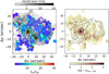 |
Fig. 17. Left: Balmer decrement measurements (purple to red) and lower limits (grey to black) across the MUSE FOV. Hα and Hβ fluxes are derived from the fitted total line profiles; 3σ upper limits for the Hβ flux are used to derive Balmer decrement lower limits. Right: E(B − V)gas map of Arp220, derived from the Hα/Hβ ratios in the top-left panel using the CCM extinction law. |
9. Neutral gas covering factor and hydrogen column densities
In this section we investigate the correlation between E(B − V)gas and cool gas absorption traced by Na ID transitions. A more detailed comparison between dust attenuation and Na ID absorption that combines the results from the analysis presented in this paper with those from Catalán-Torrecilla et al. (in prep.) will be presented in a forthcoming paper.
A positive correlation between the EW of absorbing gas and E(B − V)gas has been used as indirect evidence of dust in outflows (e.g. Shapley et al. 2003; Reichard et al. 2003; Perna et al. 2019). In particular, Rupke & Veilleux (2015) reported a positive correlation between the EW of outflowing Na ID and the stellar continuum attenuation in the ULIRG IRASF05189−2524. Following the arguments presented in their work, the colour excess and EW(NaIDabs) can, under particular conditions, be used as a proxy for NH. In fact, the attenuation calculated from E(B − V)gas can be related to NH, assuming a constant dust-to-gas ratio (e.g. in the Milky Way, NH/E(B − V) = 6.9 × 1021 cm−2; Güver & Özel 2009). Similarly, when the absorbing neutral material has a low optical depth (τ < 1) and a uniform and total coverage of the continuum source (Cf = 1), the EW(NaIDabs) is proportional to NH (e.g. Rupke et al. 2005a). Following Cazzoli et al. (2016), we considered the average NH–EW(NaIDabs) relation within the two extreme relationships – found by Turatto et al. (2003) and derived from SN reddening measurements – to obtain the empirical equation
 (4)
(4)
In Fig. 18 (top left) we report the measured EW(NaIDabs) as a function of E(B − V)gas. The measurements are colour-coded using the ELR function of the [N II]-BPT diagram; the dashed line displays Eq. (4). This figure shows that our measurements follow the predicted relation regardless of the ionisation mechanisms responsible for the line emission. In support of the observed correlation, we note that our fit results tend to favour low τ and high Cf: The median covering factor and the optical depths observed across the MUSE FOV are  and
and  (see Fig. 18, top right).
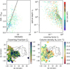 |
Fig. 18. Top left: E(B − V)gas as a function of the Na ID EW. The dashed line represents Eq. (4), derived under the assumption that both quantities are proportional to the hydrogen column density NH. Top right: covering factor vs. optical depth for each kinematic component used to model the Na ID profiles. The points in the top panels are colour-coded according to their position in the [N II]-BPT diagram (Fig. 14, top right). Bottom left: covering factor map, obtained from the total Na ID profiles following the Rupke et al. (2005a) prescription. Bottom right: column density map, obtained by summing the NH derived from each kinematic component required to model Na ID profiles. |
Finally, following the prescriptions reported in Rupke et al. (2005a), we derived the sodium abundance, taking into account the ionisation fraction (y = 0.9) and the depletion of Na atoms onto dust and the abundance, as
 (5)
(5)
where A = log(NNa/NH)gal is the Na abundance in the galaxy, and B = log(NNa/NH)−log(NNa/NH)gal = −0.95 is the depletion (the canonical Galactic value, Savage & Sembach 1996). Using the galaxy abundance derived from Eq. (12) in Rupke et al. (2005a), A = −5.4, we derived the column densities reported in Fig. 18 (bottom right). These measurements are obtained from the sum of all the kinematic component contributions and are consistent with column densities generally derived from outflowing Na ID gas (e.g. Rupke & Veilleux 2015; Cazzoli et al. 2016; Perna et al. 2019; Catalán-Torrecilla et al. 2020; see also Veilleux et al. 2020). Column densities of the order of 0.5 − 5 × 1021 cm−2 were also derived from X-ray Chandra data within the innermost kpc by Huo et al. (2004) and Grimes et al. (2005).
10. Outflow characterisation
In this section we derive the general properties of the outflowing gas using the information collected so far. We propose two possible outflow configurations, namely a collimated and a wide-angle biconical outflow, and derive their energetics assuming simple mass-conserving wind models.
10.1. Outflow structure
For each individual Gaussian set used to model the line profiles, [N II]-, [S II]-, and [O I]-BPT diagrams were used to distinguish between SF and shock ionisation. In particular, a Gaussian set is associated with SF ionisation if at least two BPT diagrams indicate HII-like ratios; on the other hand, a Gaussian set is associated with shock ionisation when line ratios in all BPT diagrams are in the LI(N)ER regions. Star formation and shock Gaussian sets were then used to construct two data cubes containing the best-fit SF- and shock-[N II] profiles, respectively. These data cubes were used to generate the [N II] velocity channel maps presented in Fig. 19, for both shock excitation (top panels) and SF ionisation (bottom). In the following, we describe the main features observed in individual velocity channels.
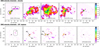 |
Fig. 19. [N II] velocity channels extracted from the data cubes containing the best-fit profiles of shock (top) and SF-ionised (bottom) gas. Letters from A to J locate the main kinematic structures discussed in Sect. 10; in the bottom panels, we also mark the position of the four SCs. |
[−625, −375] km s−1: Fast approaching gas is mostly associated with shocks. This shock-excited gas is preferentially found in the innermost nuclear regions, where we observe two bright clumps within the bubble (∼2″ north-west of the nuclei) and along two main filaments (A and B regions in the panel). In the SF emission map, we observe some diffuse gas in the north-west quadrant (C region), as well as a few Voronoi bins of faint emission towards the south-east.
[−375, −125] km s−1: The distribution of shock-induced emission is very similar to the distribution in the previous velocity channel; the western part of the lobe is identified (D region). We also find high-v gas in the south-west quadrant (E region). In the SF map, we identify the two clumps of SF, labelled as SC3 and SC4, as well as other fainter emission preferentially aligned along PA ≈ 138° (i.e. the outflow direction).
[−125, +125] km s−1: Low-v shock-induced emission fills the bottom part of the lobe structure (F region) and appears to join the bubble with the upper part of the western lobe (G); similarly, in the south-east quadrant, low-v emission connects the nuclear regions to the high-v shocked gas (H). The SF gas is preferentially associated with the innermost nuclear regions (SC1, SC2, and SC4) but presents several clumps that are isotropically distributed across the MUSE FOV.
[+125, +375] km s−1: Shock-induced emission fills a cone with a large opening angle positioned towards the east (within the angle defined by the I and J lines). The SF gas is mostly associated with SC1 and SC2, but, again, fainter emission can be located along PA ≈ 138°.
[+375, +625] km s−1: Shock-induced emission reproduces the main features observed in the previous channels; SF emission is mostly undetected, except for a few Voronoi bins of faint emission towards the south-east.
To summarise, shock emission mostly follows a few kinematic structures. The most extreme velocities (|v|≳600 km s−1) in the ionised gas are measured along PA ∼ 138°; their spatial correlation with high-v Na ID and with X-ray emission, and their alignment with the minor axis of the stellar disc, suggest the presence of a collimated outflow driven by nuclear SB and/or AGN activity. It is still unclear, however, if this ejected gas is part of a more structured outflow morphology, for example also involving some of the structures presented in Fig. 19.
In the following, we propose that the high-v gas in Arp220 might also be associated with a wide-angle biconical outflow. We anticipate, however, that the collimated outflow scenario will be preferred because of the arguments presented at the end of this section. Figure 20 shows a three-colour image of [N II] shock emission, where high-v approaching and receding gases are shown in blue and red, respectively, while low-v gas is shown in green. In the figure we also marked the regions associated with the main dust lanes with cyan curves, which, in our proposed scenario, affect the outflow path; these same regions can be easily identified in the inset, which shows the blue stellar continuum emission – and the dust filaments with flux deficiency – from HST/F436M observations.
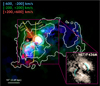 |
Fig. 20. Schematic view of the main structures in Arp220, revealed by MUSE. The three-colour image shows the [N II] shock emission, reconstructed from multi-component best-fit results. Superimposed yellow lines highlight the biconical outflow. Star symbols identify the four main SCs identified in Sect. 10. Cyan curves locate the main dust filaments possibly affecting the outflow geometry. The same curves are reported in the inset, showing the blue stellar continuum emission as well as the dusty structures in the innermost nuclear regions of Arp220. |
In the eastern part of the FOV, there could be a one-sided and wide-angled kpc-scale conical outflow that expands in a clumpy medium. The fast receding gas defines the edges of a cone well (I and J lines in Fig. 19, top right); along the cone axis there are both low-v blue-shifted and red-shifted components (H region in Fig. 19). This gas is brighter than the gas at the edges of the cone (seen at faster receding velocities), indicating that the latter likely resides behind the kpc-scale disc. Instead, the gas in the H region likely propagates close to the plane of the sky, as it is associated with velocities from ≈ − 600 to ≈ + 600 km s−1. This gas could be confined by the dust lane extending along the south-eastern direction from the nuclei towards the south-west at r ∼ 10″ (see Fig. 20). The dust distribution may possibly deviate the outflow direction towards a path closer to the LOS, generating the comma-shaped region (A) with high-v approaching gas (up to ≈ − 1000 km s−1).
This scenario is also consistent with the neutral outflow kinematics traced by Na ID gas (Figs. 11 and 12). Blue-shifted absorbing material with high W80 is revealed along PA ∼ 138° in the south-east quadrant; importantly, P-Cygni profiles are found in the more external regions, along the lower edge of the cone, where we observe both blue-shifted (v < −300 km s−1) and red-shifted (v > 200 km s−1) ionised gas. Na ID emission therefore traces the more distant receding outflowing gas, which is less attenuated by the dust with respect to the innermost regions; Na ID absorption is instead related to the foreground-approaching outflowing material.
In support of this scenario, we note that the distribution of receding and approaching gas in Arp220 is very similar to those in the Circinus galaxy and NGC 4945 once we consider a different (opposite) LOS (see e.g. Mingozzi et al. 2019, Fig. 2; Venturi et al. 2017, Fig. 2). The presence of higher velocities at the edges of the cone can be explained by projection effects, assuming they are mostly perpendicular to the plane of the sky. Instead, the higher velocity dispersions along the cone axis, due to the presence of both approaching and receding ionised gas, can be explained by considering a cone axis close to the plane of the sky.
In the western part of the FOV, the shock emission is dominated by the bubble. This structure may have originated from the counterpart of the eastern outflow cone, which is confined by the dust lanes observed in the HST images (see Fig. 20). The lobe structure could have originated from outflowing gas, which, at larger distances, starts to flow back to the interacting system. Alternatively, it might have originated from the interaction of the merging galaxies, as suggested by the presence of tidal tails in the merger simulations presented in König et al. (2012).
The information collected so far, however, does not allow us to robustly discriminate between tidally and outflow-induced shocks at low to intermediate (∼500 km s−1) velocities; moreover, the locations of dust and ejected gas along the LOS are unconstrained, and we do not know if the dust is actually deviating the outflow path. Therefore, in the following, we refer to the collimated outflow geometry as the preferred scenario.
10.2. Location of the outflow origin
Even with the present AO-assisted IFS data, we cannot accurately locate the origin of the kpc-scale outflow that we detect in atomic ionised and neutral gas. However, a few considerations can be made taking into account the high-resolution (∼0.1″) ALMA observations that trace the HCN (1–0) and HCO+ (1–0) emission lines in the surroundings of the two nuclei, which are presented in Barcos-Muñoz (2016) and Barcos-Muñoz et al. (2018). The authors report the detection of a spatially resolved molecular outflow associated with the W nucleus, with an extension of ≲120 pc along the north-south direction. The kpc-scale atomic outflow we present in this paper is unlikely to be related to the molecular wind in the W nucleus, as it is preferentially oriented along PA ∼ 138°.
Recently, Wheller et al. (2020) reported evidence for a collimated outflow in the E nucleus, traced by CO(3–2) at high resolution (∼0.2″) with ALMA observations. This outflow is oriented along the kinematic minor axis of the nuclear molecular disc and extends out to ≲100 pc from the E nucleus. These findings might suggest that such a nuclear wind is related to the kpc-scale atomic outflow presented in this paper. This scenario, however, has to be confirmed with follow-up observations, for example by tracing atomic gas kinematics through IR transitions, which are less affected by dust extinction emission lines, with high angular resolution.
10.3. Outflow energetics
The construction of a detailed 3D kinematic model for the Arp220 outflow is beyond the scope of this paper. In this section, we derive order-of-magnitude estimates of the outflow energetics assuming simple mass-conserving wind models. Inclination-corrected velocities and distances are obtained assuming that the outflow is oriented on the plane of the E nucleus disc (see Sect. 10.2) with an inclination of 70° to the LOS (e.g. Scoville et al. 2017).
We calculated the outflow mass rate of the ionised gas in each Voronoi bin from the de-reddened flux of the Hα components associated with non-SF ionisation, assuming the Case B recombination in fully ionised gas with Te = 104 K (see e.g. Cresci et al. 2017) and a uniform electron density across the MUSE FOV, Ne = 170 cm−3 (Sect. 7). We performed the outflow mass rate calculation for each Voronoi bin using the relation Ṁ = Moutvout/Rout, with vout = v50 (e.g. Harrison et al. 2014), and considering the respective local properties (e.g. velocities, Hα flux, and distance from the nuclear regions). We thus obtained the total ionised outflow mass rate and the kinetic ( ) and moment power (Ṗ = Ṁvout) by summing the values from the single Voronoi bins: Ṁ = 20 M⊙ yr−1,
  erg s−1, and Ṗ = 4 × 1034 dyne9. For each outflow energetic, we also derived a confidence interval (CI), considering most and least conservative assumptions and taking into account an Ne in the range [60,440] cm−3 (Sect. 7) as well as the fact that Hα emission at |v| < 375 km s−1 may or may not participate in the outflow (Sect. 10.1): We obtained Ṁ ∈ [5,60] M⊙ yr−1,
 ![Mathematical equation: $ \dot K \in [0.5,7]\times 10^{42} $](/articles/aa/full_html/2020/11/aa38328-20/aa38328-20-eq15.gif) erg s−1, and Ṗ ∈ [0.9,9] × 1034 dyne.
erg s−1, and Ṗ ∈ [0.9,9] × 1034 dyne.
We calculated the outflow energetics of the neutral gas traced by Na ID absorption assuming the same wind model and following the arguments presented in Shih & Rupke (2010). We excluded, here as well, the kinematic components associated with SF-ionisation and performed a Gaussian smooth (with σ = 2 pixels) on the NH map (Fig. 18) to remove a few outlier measurements that were (probably) due to unphysical values associated with τ ≫ 110. To further limit the possible inclusion of gas that does not participate in the outflow, we considered only the kinematic components with v < −50 km s−1 (e.g. Rupke et al. 2005b). We assumed a single radius for the wind, Rout = 6 kpc (which roughly corresponds to the distance of the comma-shaped region), and used the NH, Cf and velocities from individual Voronoi bins. The total outflow energetics are: Ṁ = 27 M⊙ yr−1,  erg s−1, and Ṗ = 1035 dyne. As for the ionised component, we also derived a CI considering most and least conservative assumptions: Ṁ ∈ [2,40] M⊙ yr−1,
 ![Mathematical equation: $ \dot K = [0.7,6]\times 10^{42} $](/articles/aa/full_html/2020/11/aa38328-20/aa38328-20-eq17.gif) erg s−1, and Ṗ = [0.1,2] × 1035 dyne. The minimum values were computed considering only the Voronoi bins with W80 > 700 km s−1 (roughly corresponding to the selection of the Na ID profiles extended at v < −375 km s−1, as for the ionised component); the maximum values were obtained considering an outflow radius of 9 kpc (see e.g. Fig. 12). All the outflow energetics computed so far are reported in Table 2.
erg s−1, and Ṗ = [0.1,2] × 1035 dyne. The minimum values were computed considering only the Voronoi bins with W80 > 700 km s−1 (roughly corresponding to the selection of the Na ID profiles extended at v < −375 km s−1, as for the ionised component); the maximum values were obtained considering an outflow radius of 9 kpc (see e.g. Fig. 12). All the outflow energetics computed so far are reported in Table 2.
Outflow properties.
Our results suggest that the neutral and ionised outflows in Arp220 likely have similar mass rates and energetics and are consistent with other AGN- and SB-driven outflows at low z (e.g. Rupke et al. 2017; Fluetsch et al. 2019, 2020). In Table 2 we also report the relative contributions associated with the main outflow features in Arp220: the bubble and the comma-shaped region along PA ∼ 138°. A significant portion of the ionised outflow mass, energy, and momentum rates are associated with the bubble, which is closer to the central engine of the outflow. As suggested by, for example, Venturi et al. (2018), a decrease in outflow energetics with distance might either imply that the outflow slows down at larger distances, or that the SB (AGN) pushing the wind has recently become more powerful. Another possible explanation could be related to projection effects. In order to better characterise the outflow properties, a more detailed wind model is therefore required.
The values reported in Table 2 also suggest that the possible contribution of gravitational induced shocks should be minor, as a significant fraction of the outflow kinetic energy derived from the ionised and neutral gas components is associated with the two brightest structures in Arp220: the bubble and the comma-shaped region, which also present the most extreme kinematics (barely attributable to tidally induced shocks).
10.4. Outflow launch mechanism(s)
In order to investigate the possible origin of the outflow, we compared our inferred values of the total outflow energetics with the expected kinetic and momentum power ascribed to stellar processes. The expected rate of energy injection from SN explosions is ∼1044 erg s−1, and it has been derived assuming the standard SN energy, KSN = 1051 erg, and considering the Arp220 SN rate of 4 yr−1 (Varenius et al. 2019). This expected kinetic power is very similar to that derived assuming a proportionality between  and the SFR (Veilleux et al. 2005),
  erg s−1, taking into account the Arp220 SFR of 250 M⊙ yr−1 (Nardini et al. 2010). The measured
  suggests a ≈4% coupling between the stellar processes and the wind energy, which is consistent with the one expected for SB-driven outflows (e.g. Chevalier 1974; Schneider et al. 2020). Similarly, the mass-loading factor μ = Ṁout/SFR = 0.2 is similar to those measured in other local ULIRGs (Arribas et al. 2014; Chisholm et al. 2017; Cresci et al. 2017) and high-z star-forming galaxies (Genzel et al. 2014; Newman et al. 2012; Perna et al. 2018) with SB-driven outflows. However, the momentum rate generally observed in SB-driven outflows is ≳10 times smaller than the one derived for Arp220 (see e.g. Fluetsch et al. 2019, Fig. 20; Cicone et al. 2014, Fig. 16).
We also compared our inferred outflow properties with the expected kinetic and momentum power expected for AGN-driven outflows. We tentatively estimated the expected rate of energy from CT AGN considering the AGN luminosities inferred by Paggi et al. (2017) and Nardini et al. (2010), from X-ray and IR data, respectively (see Sect. 2). We derived the bolometric LAGN > 1044 erg s−1 (W) and > 3 × 1044 erg s−1 (E) from the two lower limits L2 − 10 keV of the two nuclei, considering a bolometric correction KX ∼ 11.5 (Duras et al. 2020). These estimates translate to the upper limit  for the W nucleus and to
  for the E nucleus. On the other hand, the average IR-based bolometric AGN luminosity, of the order of ∼1.7 × 1045 erg s−1, allows us to obtain a
  and a momentum rate ratio Ṗ/(LAGN/c) ∼ 0.74, consistent with other AGN-driven outflows at low z (e.g. Cicone et al. 2014; Fluetsch et al. 2019, 2020), as well as with theoretical predictions (e.g. Harrison et al. 2018).
Therefore, the inferred outflow energetics are consistent overall with both AGN- and SB-driven expectations and cannot be used to infer the outflow origin (i.e. whether they are AGN-driven or SB-driven). Finally, we also stress that the energetics should be considered as rough estimates because of the assumed simple wind model, which could not describe the complex kinematics observed in Arp220 well. Moreover, further, deeper multi-wavelength observations are required to better constrain the AGN bolometric luminosity, as well as the IR luminosity and SFR for the two individual nuclei (e.g. Paggi et al. 2017; Dwek & Arendt 2020).
10.5. Negative feedback
In general, if outflow velocities are high enough to escape the potential of the galaxy, then galactic outflows can effectively clear the galaxy of its gas content (“ejective feedback”; e.g. Nelson et al. 2019). However, this mechanism could be inefficient in Arp220, as a significant fraction of the outflowing material could collide with tidal streams and infalling gas.
In such conditions, the “preventive feedback” (e.g. Pillepich et al. 2018; Cresci & Maiolino 2018) could represent a more efficient mechanism: In this scenario, the formation of new stars is limited by the injection of outflow energy, which heats the gas and prevents it from cooling. The ubiquitous detection of powerful, kpc-scale outflows in merging systems (eg. Feruglio et al. 2015; Rupke & Veilleux 2013, 2015; Saito et al. 2018; Perna et al. 2019) could suggest a significant impact of AGN and SB outflows already present from the early phases of the formation of massive galaxies (see also e.g. Arribas et al. 2014).
11. SF activity and evidence for positive feedback
In Fig. 21 we report the distribution of gas ionised by young and massive stars that is traced by Hα emission. This map has been constructed on the basis of our multi-component best-fit results, selecting the Gaussian components associated with SF ionisation, according to at least two BPT diagnostics (Fig. 14). All fluxes in the figure have been corrected for dust attenuation using the E(B − V)gas measurements and a CCM extinction law (Sect. 8). The map highlights the presence of at least four bright clumps, which were already identified in Sects. 6 and 10, with diameters ranging from ∼400 pc (SC2) to ∼700 pc (SC4) and associated with SFR from ≈0.1 M⊙ yr−1 to 2.8 M⊙ yr−1 (using the Kennicutt 1998 relation). The main properties of these SCs, reported in Table 3, follow the expected empirical relationships between the velocity dispersion, size, and luminosity of stellar clumps in local and high-z galaxies (see e.g. Fig. 8 in Arribas et al. 2014).
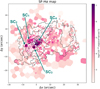 |
Fig. 21. Distribution of gas ionised by young and massive stars, traced by Hα emission. All fluxes have been corrected for dust attenuation. See Sect. 11 for details. |
SF clumps properties.
The integrated spectra of the four clumps are reported in Appendix F. We fitted these spectra to derive the main properties of the atomic gas ionised by young stars, following the prescriptions presented in previous sections. In particular, we mention here that the N2-based (e.g. Curti et al. 2017) metallicities in the main stellar clumps are 12 + log(O/H) ≳ 8.6, consistent with those of ULIRG SF regions (8.5 < 12 + log(O/H) < 8.9, from Pereira-Santaella et al. 2017). In summary, not only do the BPT diagnostic diagrams suggest SF-like ionisation, but the properties of these SCs (i.e size, velocity dispersion, luminosity, and metallicity) also correspond to those observed in other stellar clumps in local ULIRGs.
The derived SFRs associated with these clumps are two orders of magnitude lower than the one derived from LIR. The integrated Hα emission in Fig. 21 corresponds to a total SFR ≲ 10 M⊙ yr−1. This suggests the presence of additional highly obscured SF regions in the innermost nuclear part of Arp220. We stress that the detection of SF components in MUSE data is made even more difficult because of shocks, whose emission dominates over the SF ionisation in optical lines.
11.1. Positive feedback: SF by outflow-induced pressure
The stellar clumps SC2 and SC4 are located at the edge of the outflow regions (see star symbols in Fig. 20); moreover, the gas velocities within these SCs significantly deviate from those of the main stellar component. Similar spatial configuration between outflowing gas and SF regions has been already reported in other systems, both at low z (e.g. Cresci et al. 2015b; Maiolino et al. 2017; Shin et al. 2019; Cicone et al. 2020) and at z > 1 (e.g. Cresci et al. 2015a; Carniani et al. 2016; but see also Scholtz et al. 2020). These indications have been interpreted as possible evidence for SF triggered by outflows (e.g. Cresci & Maiolino 2018): In this scenario, the outflows compress the ISM at its edges, enhancing the formation of new stars with high velocities.
11.2. Positive feedback: SF within the outflow
A different scenario can be proposed for SC3. This clump presents the most extreme gas velocities (V ≈ −230 km s−1), clearly decoupled from the global stellar component (with velocities in the range V* ∈ [ − 130, +130] km s−1 over the entire MUSE FOV). Moreover, unlike SC2 and SC4, this clump is located well within the outflow region. We also note that when SF emission is split in velocity channels (Fig. 19, lower panels), the presence of faint and clumpy SF, in addition to the SCs, is revealed. This emission is preferentially found along the outflow direction (i.e. PA ∼ 138°) for the most extreme velocities, showing additional evidence that SF may be associated with the outflow. Its detection, however, has lower significance than in SC3, as it is strongly dependent on our best-fit analysis: stronger degeneracies between individual kinematic components might be present where the line profiles are more complex.
Our results are consistent with those reported for other nearby sources (Maiolino et al. 2017; Gallagher et al. 2019; Rodríguez del Pino et al. 2019) and suggest that AGN and SB winds can ignite SF within the outflow itself, consistent with predictions from models and recent numerical simulations (e.g. Ishibashi et al. 2013; Zubovas et al. 2013; Zubovas & King 2014; Decataldo et al. 2019; Yu et al. 2020). Quantitatively, this represents only a small amount (∼2%) of the SFR inferred from the total LIR, which is slightly at odds with the results from Gallagher et al. (2019), who detected widespread SF inside MaNGA galaxy outflows with rates between 5% and 30% of the total SFR. We argue that this mild inconsistency could be explained considering the difficulties in detecting SF ionisation in Arp220 due to the ubiquitous presence of shocks, whose emission dominates in the emission line profiles.
11.3. Evidence for in situ SF within the SCs
One potential concern regarding the positive feedback scenario is that the main clumps of SF-ionised gas have been isolated on the basis of BPT line ratios. Such diagnostics do not provide direct evidence of the presence of young stars within the SCs: Stars in the galaxy disc can potentially ionise their gas (i.e. from the outside) and produce the line ratios observed in the SC-integrated spectra (Fig. F.1). Therefore, we need to discriminate between in situ and external photoionisation for individual clumps.
In the scenario of in situ SF, one would expect that the ionising flux in SCs would be similar to those in standard SF regions, while the electron density Ne would be similar to (or even higher than) those in the unperturbed ISM (e.g. Sect. 3.2 in Gallagher et al. 2019). We derived the ionisation parameter for each clump, analysing their integrated spectra and isolating the Gaussian components associated with SF. The derived log U, reported in Table 3, are consistent with those reported by Maiolino et al. (2017), Gallagher et al. (2019), and Rodríguez del Pino et al. (2019) for stellar clumps in other AGN-driven outflows, as well as those of standard SDSS star-forming regions. The electron densities in individual stellar clumps are compatible with (or even higher than) the median Ne measured across the MUSE FOV. Therefore, both log U and Ne are consistent with the scenario of in situ photoionisation of the gas.
All results reported so far are compatible with the finding of SF triggered by the outflow reported in the literature: Although we cannot exclude that these SCs are simple star-forming regions in the interacting system, their peculiar kinematics and their locations with respect to the outflowing gas support the positive feedback scenario. Even if the SFR in the outflow is low compared with the global SFR in the whole system, one should take into account that stars formed inside the outflow have kinematics that are completely different from those formed in the galaxy discs, in the sense that they have highly radial orbits and therefore can potentially contribute significantly to the formation and growth of the spheroidal component of the galaxy. A more detailed investigation is, however, required to confirm the origin of the SCs in Arp220.
12. Conclusions
We have presented recent MUSE-AO observations of Arp220, a prototypical ULIRG and late-stage merger with dominant SF in the centre (Nardini et al. 2010) and kpc-scale warm gas emission in plumes and lobes (e.g. McDowell et al. 2003; Arribas et al. 2001; Colina et al. 2004). We produced high-resolution (∼0.56″, 210 pc) maps of stellar and gas kinematics and studied the state of the ionised and neutral gas.
The main results inferred from the modelling of the stellar kinematics, and the characterisation of the systemic ISM (i.e. not perturbed by the outflow), are summarised as follows.
-
We observed a velocity gradient along the north-east – south-west direction (PA ∼ 48°) in the stellar (gas) velocity maps, with amplitudes of ≈ ± 100 km s−1 (≈ ± 200 km s−1). However, gas and stars are still strongly disturbed and have not yet settled into a galactic plane. High-v tidal structures at projected distances > 10″ (3.7 kpc) are observed in both stellar kinematics (with velocity amplitudes up to ±130 km s−1) and ionised and neutral gas (up to ±300 km s−1).
-
Spatially resolved BPT diagnostics have been used to locate SF regions. A significant fraction of stellar Hα emission comes from four clumpy regions within the innermost nuclear regions (r < 10″); additional diffuse Hα emission is found across the MUSE FOV. The total SFR inferred from stellar Hα (≲10 M⊙ yr−1) is one order of magnitude lower than the IR-based SFR ∼ 250 M⊙ yr−1. This suggests that most of the SF activity in Arp220 is highly obscured.
-
We measured [S II]-based average electron densities of the order of ≈170 cm−3. This result suggests similar conditions in the ISM gas for local ULIRGs and high-z star-forming galaxies.
-
The E(B − V)gas and the EW of Na ID absorbing gas can be used as a proxy for the hydrogen column density in Arp220, as suggested by the correlation between E(B − V)gas and EW(NaIDabs). This correlation is observed in SF regions as well as in those with clear evidence of outflows; moreover, it is also consistent with the empirical relations by Turatto et al. (2003), derived from ISM lines in SN spectra.
The high-resolution wide-field MUSE-AO observations have also allowed us to characterise the kpc-scale outflow in Arp220 in detail. Our main findings can be summarised as follows.
-
We revealed a close correspondence between the X-ray emission and the presence of extremely broad ionised and neutral gas line features along the south-east – north-west direction (PA ∼ 138°), that is, along the minor axis of the disturbed kpc-scale disc revealed in the stellar kinematic analysis.
-
Tidally induced shocks and outflows are the main phenomena responsible for ISM ionisation, as inferred from spatially resolved BPT diagnostic diagrams. This result was supplemented with comparisons of the measured line ratios and line widths with the predictions of shock models from MAPPING V. These models suggest that diffuse gas is ionised by tidally induced shocks with Vs of a few 100 km s−1, while the gas along PA ∼ 138° is associated with velocities up to ≈1000 km s−1, which could reasonably be due to SB- or AGN-driven outflows.
-
We derived the outflow energetics assuming a simple mass conserving wind model: combining the atomic neutral and ionised gas components, we obtained a mass rate Ṁ ∼ 50 M⊙ yr−1, a kinetic power
 erg s−1, a momentum power Ṗ ∼ 1035 dyne, and a mass-loading factor μ ∼ 0.2. These properties do not allow us to distinguish the origin of the outflows (i.e. whether they are SB- or AGN-driven). Nevertheless, the inferred energetics suggest that the outflow can strongly affect the evolution of the system, either through negative feedback (i.e. expelling the gas; but see Sect. 10.5) or through preventive feedback (i.e. preventing the gas from cooling and preventing the formation of new stars).
 -
We reported evidence for positive feedback in Arp220: We located two clumps of SF at the outflow edges (SC2 and SC4) with velocities clearly decoupled from the global stellar component and SFRs of 0.2 M⊙ yr−1 (SC2) and 2.8 M⊙ yr−1 (SC4). Our findings are consistent with the positive feedback scenario, according to which such clumps are formed from the compression of ISM at the outflow edges. Furthermore, we located an additional clump within the outflow, SC3, with the most extreme gas velocities (−230 km s−1 from the Arp220 systemic) and SFR ∼ 0.5 M⊙ yr−1. Such peculiar properties suggest a different and even more fascinating scenario of positive feedback: The formation of SC3 may have happened as the outflow material cooled down and fragmented, leading to the formation of new stars within the outflow, as recently reported in other systems (e.g. Maiolino et al. 2017). Interestingly, as also reported by these authors, even if the SF in these clumps is small relative to the global SF, their peculiar kinematics can potentially contribute significantly to the formation of the spheroidal component of a galaxy (e.g. Yu et al. 2020).
Our analysis shows that detailed multi-phase studies are required to characterise the outflows. Our findings emphasise the capabilities of MUSE, which allows for the simultaneous characterisation of both neutral and ionised gas in nearby galaxies. However, for a comprehensive understanding of the outflow phenomena, all different gas phases must be carefully investigated. So far, no indication of large-scale molecular outflows has been reported. This could be due to the fact that high-v molecular emission is usually more than ten times fainter than that from non-outflowing gas, and large integrations are needed even with the most sensitive millimetre/sub-millimeter interferometers (e.g. Cicone et al. 2018).
Nuclear molecular outflows have been detected in both Arp220 nuclei. Hence, we tried to combine the information from the MUSE-AO data analysis with the high-resolution (∼0.1″) ALMA observations, tracing molecular gas emission in the surroundings of the E and W nuclei (e.g. Barcos-Muñoz 2016, 2019; Wheller et al. 2020). We suggest that the galactic-scale atomic outflow is emerging from the E nucleus of Arp220, taking into account simple geometrical arguments. Direct evidence for the location of the kpc-scale outflow, however, requires dedicated follow-up observations. The JWST/NIRSpec IFS capabilities will allow for a comprehensive characterisation of the ionised and warm molecular (e.g. H21 − 0) phases of the ISM, covering the spectral range from 0.6 to 5.3 μm with a sub-arcsec resolution and a sampling of 0.1″, hence testing our proposed scenario for the location of the origin of the kpc-scale atomic outflow. Furthermore, JWST/MIRI observations will be key to finding direct evidence of dust-obscured AGN in the two nuclei.
Starting from the astrometry derived from the EsoReflex pipeline, we had to apply a correction of ΔRA = −2.1″ and ΔDec = 0.8″; no rotational term has been taken into account.
The STAT data cube produced by the EsoReflex pipeline is used to define the flux errors.
[O III] and Hβ emission along the dust lane and at r ≳ 10″ from the nuclei could be below the sensitivity of the HST images used to derive the [O III]/Hβ map in Lockhart et al. (2015).
The STAT data cube produced by the EsoReflex pipeline is used to set the standard deviations of the Gaussian distributions from which a random noise is extracted.
Using the whole Na ID profile, v50 velocity would be red-shifted, on average, by ∼ + 100 ± 35 km s−1 (with respect to the H transition zero-velocity), while W80 values would increase, on average, by 190 ± 50 km s−1.
The EW is defined as ∫(1 − fline/fcon)dλ, where the fline and fcon indicate the line and the continuum flux, respectively. The EW is defined for absorption line systems and is therefore negative for emission features. Throughout the paper, we implicitly refer to its absolute value.
In many local galaxies, the LI(N)ER emission is associated with gas ionised by the hard radiation field of evolved (post-AGB) stars, as discussed e.g. in Belfiore et al. (2016). However, this likely does not apply to SB galaxies such as Arp220.
These flux ratios were obtained using the [O III]-based Voronoi tessellation; a more uniform coverage of the circum-nuclear regions could be obtained using an [S III]-based binning without affecting outcomes shown in the figure.
These values are consistent (within a few percentage points) with those derived from integrated quantities, considering an outflow extension of 6 kpc (see also Venturi et al. 2018).
This is the same as removing all Voronoi bins with τ > 7 from the energetics computation.
Acknowledgments
We thank the referee for an expert review of our paper. MP thanks A. Pensabene, M. Mingozzi, G. Venturi, S. Quai, G. Vietri, A. Puglisi, L. Costantin, D. Baron, G. Cresci, M. Brusa and R. Marques-Chaves for fruitful discussions regarding different aspects presented in this manuscript. MP is supported by the Programa Atracción de Talento de la Comunidad de Madrid via grant 2018-T2/TIC-11715. MP, SA, CTC and LC acknowledge support from the Spanish Ministerio de Economía y Competitividad through the grant ESP2017-83197-P, and PID2019-106280GB-I00. MPS acknowledges support from the Comunidad de Madrid through the Atracción de Talento Investigador Grant 2018-T1/TIC-11035. SC acknowledges financial support from the State Agency for Research of the Spanish MCIU through the “Center of Excellence Severo Ochoa” award to the Instituto de Astrofísica de Andalucía (SEV-2017-0709). AF and RM acknowledge ERC Advanced Grant 695671 “QUENCH” and support by the Science and Technology Facilities Council (STFC). EB acknowledges the support from Comunidad de Madrid through the Atracción de Talento grant 2017-T1/TIC-5213. JPL acknowledges financial support by the Spanish MICINN under grant AYA2017-85170-R. This paper makes use of data from the ESO Multi Unit Spectroscopic Explorer (MUSE) observing programme 0103.B-0391(A), available for download from the ESO archives: https://archive.eso.org/eso/eso_archive_main.html, for raw data, and http://archive.eso.org/wdb/wdb/adp/phase3_main/form, for reduced data.
References
- Aalto, S., Martín, S., Costagliola, F., et al. 2015, A&A, 584, A42 [NASA ADS] [CrossRef] [EDP Sciences] [Google Scholar]
- Alarie, A., & Morisset, C. 2019, Rev. Mex. Astron. Astrofís., 55, 377 [Google Scholar]
- Allen, M. G., Groves, B. A., Dopita, M. A., et al. 2008, ApJS, 178, 20 [Google Scholar]
- Arp, H. C., Burbidge, E. M., Chu, Y., & Zhu, X. 2001, ApJ, 553, 11 [NASA ADS] [CrossRef] [Google Scholar]
- Arribas, S., Colina, L., & Clements, D. 2001, ApJ, 560, 160 [NASA ADS] [CrossRef] [Google Scholar]
- Arribas, S., Colina, L., Alonso-Herrero, A., et al. 2012, A&A, 541, A20 [NASA ADS] [CrossRef] [EDP Sciences] [Google Scholar]
- Arribas, S., Colina, L., Bellocchi, E., et al. 2014, A&A, 568, A14 [NASA ADS] [CrossRef] [EDP Sciences] [Google Scholar]
- Bacon, R., Accardo, M., Adjali, L., et al. 2010, SPIE Conf. Ser., 7735, 773508 [Google Scholar]
- Baldwin, J. A., Phillips, M. M., & Terlevich, R. 1981, PASP, 93, 5 [NASA ADS] [CrossRef] [EDP Sciences] [Google Scholar]
- Barcos-Muñoz, L. 2016, PhD Thesis, University of Virginia, USA [Google Scholar]
- Barcos-Muñoz, L. 2019, https://doi.org/10.5281/zenodo.3585346 [Google Scholar]
- Barcos-Muñoz, L., Leroy, A. K., Evans, A. S., et al. 2015, ApJ, 799, 10 [Google Scholar]
- Barcos-Muñoz, L., Aalto, S., Thompson, T. A., et al. 2018, ApJ, 853, 28 [NASA ADS] [CrossRef] [Google Scholar]
- Baron, D., & Netzer, N. 2019, MNRAS, 486, 4290 [NASA ADS] [CrossRef] [Google Scholar]
- Baron, D., Netzer, N., Davies, R. I., & Prochaska, J. X. 2020, MNRAS, 494, 5396 [Google Scholar]
- Belfiore, F., Maiolino, R., Maraston, C., et al. 2016, MNRAS, 461, 3111 [Google Scholar]
- Belfiore, F., Westfall, K. B., Schaefer, A., et al. 2019, ApJ, 158, 160 [NASA ADS] [CrossRef] [Google Scholar]
- Bellocchi, E., Arribas, S., Colina, L., & Miralles-Caballero, D. 2013, A&A, 557, A59 [NASA ADS] [CrossRef] [EDP Sciences] [Google Scholar]
- Brusa, M., Bongiorno, A., Cresci, G., et al. 2015, MNRAS, 446, 2394 [NASA ADS] [CrossRef] [Google Scholar]
- Cappellari, M. 2017, MNRAS, 466, 798 [NASA ADS] [CrossRef] [Google Scholar]
- Cappellari, M., & Copin, Y. 2003, MNRAS, 342, 345 [NASA ADS] [CrossRef] [Google Scholar]
- Cappellari, M., & Emsellem, E. 2004, PASP, 116, 138 [NASA ADS] [CrossRef] [Google Scholar]
- Cardelli, J. A., Clayton, G. C., & Mathis, J. S. 1989, ApJ, 345, 245 [NASA ADS] [CrossRef] [Google Scholar]
- Carniani, S., Marconi, A., Maiolino, R., et al. 2016, A&A, 591, A28 [NASA ADS] [CrossRef] [EDP Sciences] [Google Scholar]
- Catalán-Torrecilla, C., Castillo-Morales, A., Gil de Paz, A., et al. 2020, ApJ, 890, 5 [CrossRef] [Google Scholar]
- Cazzoli, S., Arribas, S., Maiolino, R., & Colina, L. 2016, A&A, 590, A125 [NASA ADS] [CrossRef] [EDP Sciences] [Google Scholar]
- Cicone, C., Maiolino, R., Sturm, E., et al. 2014, A&A, 562, A21 [NASA ADS] [CrossRef] [EDP Sciences] [Google Scholar]
- Cicone, C., Brusa, M., Ramos Almeida, C., et al. 2018, Nat. Astron., 2, 176 [Google Scholar]
- Cicone, C., Maiolino, R., Aalto, S., et al. 2020, A&A, 633, A163 [CrossRef] [EDP Sciences] [Google Scholar]
- Cid, Fernandes R., Stasińska, G., Schlickmann, M. S., et al. 2010, MNRAS, 403, 1036 [NASA ADS] [CrossRef] [Google Scholar]
- Chen, Y. M., Tremonti, C. A., Heckman, T. H., et al. 2010, AJ, 140, 445 [NASA ADS] [CrossRef] [Google Scholar]
- Chevalier, R. A. 1974, ApJ, 188, 501 [NASA ADS] [CrossRef] [Google Scholar]
- Chisholm, J., Tremonti, C. A., Leitherer, C., & Chen, Y. 2017, MNRAS, 469, 4831 [NASA ADS] [CrossRef] [Google Scholar]
- Colina, L., Arribas, S., & Clements, D. 2004, ApJ, 602, 181 [NASA ADS] [CrossRef] [Google Scholar]
- Concas, A., Popesso, P., Brusa, M., et al. 2019, A&A, 622, A188 [NASA ADS] [CrossRef] [EDP Sciences] [Google Scholar]
- Cresci, G., & Maiolino, R. 2018, Nat. Astron., 2, 179 [NASA ADS] [CrossRef] [Google Scholar]
- Cresci, G., Mainieri, V., Brusa, M., et al. 2015a, ApJ, 799, 81 [Google Scholar]
- Cresci, G., Marconi, A., Zibetti, S., et al. 2015b, A&A, 582, A63 [NASA ADS] [CrossRef] [EDP Sciences] [Google Scholar]
- Cresci, G., Vanzi, L., & Telles, E. 2017, A&A, 604, A101 [NASA ADS] [CrossRef] [EDP Sciences] [Google Scholar]
- Curti, M., Cresci, G., Mannucci, F., et al. 2017, MNRAS, 465, 1384 [NASA ADS] [CrossRef] [Google Scholar]
- D’Agostino, J. J., Kewley, L. J., Groves, B. A., et al. 2019, MNRAS, 487, 4153 [CrossRef] [Google Scholar]
- Davies, R. L., Dopita, M. A., Kewley, L., et al. 2016, ApJ, 824, 50 [NASA ADS] [CrossRef] [Google Scholar]
- de Amorin, A. L., García-Benito, R., Cid, Fernandes R., et al. 2017, MNRAS, 471, 3727 [NASA ADS] [CrossRef] [Google Scholar]
- Decataldo, D., Pallottini, A., Ferrara, A., et al. 2019, MNRAS, 487, 3377 [NASA ADS] [CrossRef] [Google Scholar]
- De Robertis, M. M., & Osterbrock, D. E. 1986, ApJ, 301, 727 [NASA ADS] [CrossRef] [Google Scholar]
- Dey, A., Schlegel, D. J., Lang, D., et al. 2018, AJ, 157, 168 [Google Scholar]
- Díaz, A. I., Pagel, B. E. J., & Wilson, I. R. G. 1985, MNRAS, 212, 737 [NASA ADS] [CrossRef] [Google Scholar]
- Díaz, A. I., Castellanos, M., Terlevich, E., & Luisa García-Vargas, M. 2000, MNRAS, 318, 462 [NASA ADS] [CrossRef] [Google Scholar]
- Di Matteo, T., Springel, V., & Hernquist, L. 2005, Nature, 433, 604 [NASA ADS] [CrossRef] [PubMed] [Google Scholar]
- Dong, X., Wang, T., Wang, J., et al. 2008, MNRAS, 383, 581 [NASA ADS] [Google Scholar]
- Dopita, M. A., & Sutherland, R. S. 1995, ApJ, 455, 468 [NASA ADS] [CrossRef] [Google Scholar]
- Dopita, M. A., & Sutherland, R. S. 2003, Astrophysics of the Diffuse Universe (Berlin, New York: Springer) [CrossRef] [Google Scholar]
- Dopita, M. A., & Sutherland, R. S. 2017, ApJS, 229, 35 [NASA ADS] [CrossRef] [Google Scholar]
- Dopita, M. A., Payne, J. L., Filipović, M. D., & Pannuti, T. G. 2012, MNRAS, 956, 967 [Google Scholar]
- Dopita, M. A., Kewley, L. J., Sutherland, R. S., & Nicholls, D. C. 2016, Ap&SS, 361, 61 [NASA ADS] [CrossRef] [Google Scholar]
- Duras, F., Bongiorno, A., Ricci, F., et al. 2020, A&A, 636, A73 [CrossRef] [EDP Sciences] [Google Scholar]
- Dwek, E., & Arendt, R. G. 2020, ApJ, 901, 36 [CrossRef] [Google Scholar]
- Emonts, B. H. C., Colina, L., Piqueras-Lopez, J., et al. 2017, A&A, 607, A116 [NASA ADS] [CrossRef] [EDP Sciences] [Google Scholar]
- Engel, H., Davies, R. I., Genzel, R., et al. 2011, ApJ, 729, 58 [NASA ADS] [CrossRef] [Google Scholar]
- Falcón-Barroso, J., Lyubenova, M., van de Ven, G., et al. 2017, A&A, 597, A48 [NASA ADS] [CrossRef] [EDP Sciences] [Google Scholar]
- Feruglio, C., Fiore, F., Carniani, S., et al. 2015, A&A, 583, A99 [NASA ADS] [CrossRef] [EDP Sciences] [Google Scholar]
- Fiore, F., Feruglio, C., Shankar, F., et al. 2017, A&A, 601, A143 [NASA ADS] [CrossRef] [EDP Sciences] [Google Scholar]
- Fluetsch, A., Maiolino, R., Carniani, S., et al. 2019, MNRAS, 483, 4586 [NASA ADS] [Google Scholar]
- Fluetsch, A., Maiolino, R., Carniani, S., et al. 2020, MNRAS, submitted [arXiv:2006.13232] [Google Scholar]
- Föerster-Schreiber, N. M., Renzini, A., Mancini, C., et al. 2018, ApJS, 238, 21 [NASA ADS] [CrossRef] [Google Scholar]
- Gallagher, R., Maiolino, R., Belfiore, F., et al. 2019, MNRAS, 485, 3409 [Google Scholar]
- Genzel, R., Lutz, D., Sturm, E., et al. 1998, ApJ, 498, 579 [NASA ADS] [CrossRef] [Google Scholar]
- Genzel, R., Föerster-Schreiber, N. M., Rosario, D., et al. 2014, ApJ, 796, 7 [Google Scholar]
- Grimes, J. P., Heckman, T., Strickland, D., & Ptak, A. 2005, ApJ, 628, 187 [NASA ADS] [CrossRef] [Google Scholar]
- Groves, B. A., Dopita, M. A., & Sutherland, R. S. 2004, ApJS, 153, 9 [NASA ADS] [CrossRef] [Google Scholar]
- Güver, T., & Özel, F. 2009, MNRAS, 400, 2050 [NASA ADS] [CrossRef] [Google Scholar]
- Harrison, C. M., Alexander, D. M., Mullaney, J. R., & Swinbank, A. M. 2014, MNRAS, 441, 3306 [Google Scholar]
- Harrison, C. M., Alexander, D. M., Mullaney, J. R., et al. 2016, MNRAS, 456, 1195 [NASA ADS] [CrossRef] [Google Scholar]
- Harrison, C. M., Costa, T., Tadhunter, C. N., et al. 2018, Nat. Astron., 2, 198 [NASA ADS] [CrossRef] [Google Scholar]
- Harshan, A., Gupta, A., Tran, K. V., et al. 2020, ApJ, 892, 77 [CrossRef] [Google Scholar]
- Heckman, T. M. 1980, A&A, 87, 152 [Google Scholar]
- Heckman, T. M., Armus, L., & Miley, G. K. 1987, AJ, 93, 276 [NASA ADS] [CrossRef] [Google Scholar]
- Heckman, T. M., Armus, L., & Miley, G. K. 1990, ApJS, 74, 833 [NASA ADS] [CrossRef] [Google Scholar]
- Hibbard, J. E., Vacca, W. D., & Yun, M. S. 2000, AJ, 119, 1130 [NASA ADS] [CrossRef] [Google Scholar]
- Hinkle, J. T., Veilleux, S., & Rupke, D. S. N. 2019, ApJ, 881, 31 [CrossRef] [Google Scholar]
- Ho, I. T., Kewley, L. J., Dopita, M. A., et al. 2014, MNRAS, 444, 3894 [NASA ADS] [CrossRef] [Google Scholar]
- Hopkins, P. F. 2012, MNRAS, 420, 8 [Google Scholar]
- Hopkins, P. F., Hernquist, L., Cox, T. J., & Keres, D. 2008, ApJS, 175, 356 [NASA ADS] [CrossRef] [Google Scholar]
- Hung, C. L., Sanders, D. B., Casey, C. M., et al. 2014, ApJ, 791, 63 [Google Scholar]
- Huo, Z. Y., Xia, X. Y., Xue, S. J., et al. 2004, ApJ, 611, 208 [CrossRef] [Google Scholar]
- Husser, T., Kamann, S., Dreizler, S., et al. 2016, A&A, 588, A148 [NASA ADS] [CrossRef] [EDP Sciences] [Google Scholar]
- Ishibashi, W., Fabian, A. C., & Canning, R. E. A. 2013, MNRAS, 431, 2350 [NASA ADS] [CrossRef] [Google Scholar]
- Iwasawa, K., Sanders, D. B., Evans, A. S., et al. 2005, MNRAS, 357, 565 [NASA ADS] [CrossRef] [Google Scholar]
- Joshi, B. A., Appleton, P. N., Blanc, G. A., et al. 2019, ApJ, 878, 161 [CrossRef] [Google Scholar]
- Kakkad, D., Groves, B., Dopita, M., et al. 2018, A&A, 618, A6 [NASA ADS] [CrossRef] [EDP Sciences] [Google Scholar]
- Kakkad, D., Mainieri, V., Vietri, G., et al. 2020, A&A, 642, A147 [CrossRef] [EDP Sciences] [Google Scholar]
- Kauffman, G., Heckman, T. M., Tremonti, C., et al. 2003a, MNRAS, 346, 1055 [Google Scholar]
- Kauffmann, G., Heckman, T. M., White, S. D. M., et al. 2003b, MNRAS, 341, 33 [NASA ADS] [CrossRef] [Google Scholar]
- Kennicutt, R. C. 1998, ARA&A, 36, 189 [Google Scholar]
- Kewley, L. J., & Dopita, M. A. 2002, ApJS, 142, 35 [NASA ADS] [CrossRef] [Google Scholar]
- Kewley, L. J., Dopita, M. A., Sutherland, R. S., et al. 2001, ApJ, 556, 121 [Google Scholar]
- Kewley, L. J., Groves, B., Kauffmann, G., & Heckman, T. 2006, MNRAS, 372, 961 [NASA ADS] [CrossRef] [Google Scholar]
- Kewley, L. J., Maier, C., Yabe, K., et al. 2013, ApJ, 774, L10 [Google Scholar]
- King, A., & Pounds, K. 2015, ARA&A, 53, 115 [Google Scholar]
- König, S., García-Marín, M., & Eckart, A. 2012, ApJ, 754, 58 [NASA ADS] [CrossRef] [Google Scholar]
- Kormendy, J., & Ho, L. C. 2013, ARA&A, 51, 511 [Google Scholar]
- Liu, G., Zakamska, N. L., Greene, J. E., et al. 2013, MNRAS, 436, 2576 [NASA ADS] [CrossRef] [Google Scholar]
- Lockhart, K., Kewley, L. J., Lu, J. R., et al. 2015, ApJ, 810, 149 [NASA ADS] [CrossRef] [Google Scholar]
- Lonsdale, C. J., Diamond, P. J., Thrall, H., et al. 2006, ApJ, 647, 185 [NASA ADS] [CrossRef] [Google Scholar]
- Maiolino, R., Russell, H. R., Fabian, A. C., et al. 2017, Nature, 544, 202 [NASA ADS] [CrossRef] [Google Scholar]
- McDowell, J. C., Clements, D. L., Lamb, S. A., et al. 2003, ApJ, 591, 154 [NASA ADS] [CrossRef] [Google Scholar]
- McElroy, R., Croom, S. M., Pracy, M., et al. 2015, MNRAS, 446, 2186 [NASA ADS] [CrossRef] [Google Scholar]
- Mingozzi, M., Cresci, G., Venturi, G., et al. 2019, A&A, 622, A146 [NASA ADS] [CrossRef] [EDP Sciences] [Google Scholar]
- Mingozzi, M., Belfiore, F., Cresci, G., et al. 2020, A&A, 636, A42 [CrossRef] [EDP Sciences] [Google Scholar]
- Monreal-Ibero, A., Arribas, S., Colina, L., et al. 2006, ApJ, 637, 138 [NASA ADS] [CrossRef] [Google Scholar]
- Monreal-Ibero, A., Arribas, S., Colina, L., et al. 2010, A&A, 517, A28 [NASA ADS] [CrossRef] [EDP Sciences] [Google Scholar]
- Mortazavi, S. A., & Lotz, J. M. 2019, MNRAS, 487, 1551 [CrossRef] [Google Scholar]
- Naab, T., & Ostriker, J. P. 2017, ARA&A, 55, 109 [Google Scholar]
- Nardini, E., Risaliti, G., Watabe, Y., et al. 2010, MNRAS, 405, 2505 [Google Scholar]
- Nelson, D., Pillepich, A., Sringel, V., et al. 2019, MNRAS, 490, 3234 [NASA ADS] [CrossRef] [Google Scholar]
- Newman, S. F., Genzel, R., Föerster-Schreiber, N. M., et al. 2012, ApJ, 761, 43 [NASA ADS] [CrossRef] [Google Scholar]
- Ohyama, Y., Taniguchi, Y., Hibbard, J. E., & Vacca, W. D. 1999, AJ, 117, 2617 [NASA ADS] [CrossRef] [Google Scholar]
- Osterbrock, D. E., & Ferland, G. J. 2006, Astrophysics of Gaseous Nebulae and Active Galactic Nuclei (Sausalito, CA: University Science Books) [Google Scholar]
- Paggi, A., Fabbiano, G., Risaliti, G., et al. 2017, ApJ, 841, 44 [CrossRef] [Google Scholar]
- Pereira-Santaella, M., Rigopoulou, D., Farrah, D., et al. 2017, MNRAS, 470, 1218 [NASA ADS] [CrossRef] [Google Scholar]
- Pereira-Santaella, M., Colina, L., García-Burillo, S., et al. 2018, A&A, 616, A171 [NASA ADS] [CrossRef] [EDP Sciences] [Google Scholar]
- Perna, M., Lanzuisi, G., Brusa, M., et al. 2017a, A&A, 603, A99 [Google Scholar]
- Perna, M., Lanzuisi, G., Brusa, M., et al. 2017b, A&A, 606, A99 [Google Scholar]
- Perna, M., Curti, M., Cresci, G., et al. 2018, A&A, 618, A36 [NASA ADS] [CrossRef] [EDP Sciences] [Google Scholar]
- Perna, M., Cresci, G., Brusa, M., et al. 2019, A&A, 623, A171 [NASA ADS] [CrossRef] [EDP Sciences] [Google Scholar]
- Pillepich, A., Springel, V., Nelson, D., et al. 2018, MNRAS, 473, 4077 [Google Scholar]
- Prochaska, J. X., Kasen, D., & Rubin, K. 2011, ApJ, 734, 24 [NASA ADS] [CrossRef] [Google Scholar]
- Rangwala, N., Maloney, P. R., Wilson, C. D., et al. 2015, ApJ, 806, 17 [NASA ADS] [CrossRef] [Google Scholar]
- Raymond, J. C. 1979, ApJS, 39, 1 [NASA ADS] [CrossRef] [Google Scholar]
- Reichard, T. A., Richards, G. T., Hall, P. B., et al. 2003, AJ, 126, 2594 [NASA ADS] [CrossRef] [Google Scholar]
- Rich, J. A., Kewley, L. J., & Dopita, M. A. 2011, ApJ, 734, 87 [NASA ADS] [CrossRef] [Google Scholar]
- Rich, J. A., Kewley, L. J., & Dopita, M. A. 2015, ApJS, 221, 28 [NASA ADS] [CrossRef] [Google Scholar]
- Rodríguez del Pino, B., Arribas, S., Piqueras López, J., et al. 2019, MNRAS, 486, 344 [NASA ADS] [CrossRef] [Google Scholar]
- Rose, M., Tadhunter, C., Ramos, Almeida C., et al. 2018, MNRAS, 474, 128 [Google Scholar]
- Rupke, D. S. N., & Veilleux, S. 2013, ApJ, 775, 15 [Google Scholar]
- Rupke, D. S. N., & Veilleux, S. 2015, ApJ, 801, 126 [Google Scholar]
- Rupke, D. S., Veilleux, S., & Sanders, D. B. 2002, ApJ, 570, 588 [NASA ADS] [CrossRef] [Google Scholar]
- Rupke, D. S., Veilleux, S., & Sanders, D. B. 2005a, ApJS, 160, 115 [NASA ADS] [CrossRef] [Google Scholar]
- Rupke, D. S., Veilleux, S., & Sanders, D. B. 2005b, ApJS, 160, 87 [Google Scholar]
- Rupke, D. S. N., Gultekin, K., & Veilleux, S. 2017, ApJ, 850, 40 [Google Scholar]
- Saito, T., Iono, D., Ueda, J., et al. 2018, MNRAS, 475, 52 [NASA ADS] [CrossRef] [Google Scholar]
- Sakamoto, K., Scoville, N. Z., Yun, M. S., et al. 1999, ApJ, 514, 68 [NASA ADS] [CrossRef] [Google Scholar]
- Sakamoto, K., Wang, J., Wiedner, M. C., et al. 2008, ApJ, 684, 957 [NASA ADS] [CrossRef] [Google Scholar]
- Sanders, D. B., Soifer, B. T., Elias, J. H., et al. 1988, ApJ, 325, 74 [NASA ADS] [CrossRef] [Google Scholar]
- Sanders, R. L., Shapley, A. E., Kriek, M., et al. 2016, ApJ, 816, 23 [Google Scholar]
- Santoro, F., Rose, M., Morganti, R., et al. 2018, A&A, 617, A139 [NASA ADS] [CrossRef] [EDP Sciences] [Google Scholar]
- Sato, T., Martin, C. L., Noeske, K. G., et al. 2009, ApJ, 696, 214 [NASA ADS] [CrossRef] [Google Scholar]
- Savage, B. D., & Sembach, K. R. 1996, ARA&A, 34, 279 [NASA ADS] [CrossRef] [Google Scholar]
- Schneider, E. E., Ostriker, E. C., Robertson, B. E., & Thomas, T. A. 2020, ApJ, 895, 43 [CrossRef] [Google Scholar]
- Scholtz, J., Harrison, C. M., Rosario, D. J., et al. 2020, MNRAS, 492, 319 [NASA ADS] [CrossRef] [Google Scholar]
- Schwarz, G. 1978, Ann. Stat., 6, 461 [Google Scholar]
- Scoville, N. Z., Yun, M. S., & Bruant, P. M. 1997, ApJ, 484, 702 [NASA ADS] [CrossRef] [Google Scholar]
- Scoville, N. Z., Evans, A. S., Dinshaw, N., et al. 1998, ApJ, 492, 107 [NASA ADS] [CrossRef] [Google Scholar]
- Scoville, N., Sheth, K., Walter, F., et al. 2015, APJ, 800, 70 [Google Scholar]
- Scoville, N., Murchikova, L., Walter, F., et al. 2017, ApJ, 836, 66 [Google Scholar]
- Shapley, A. E., Steidel, C. C., Pettini, M., & Adelberger, K. L. 2003, ApJ, 588, 89 [Google Scholar]
- Shimizu, T. T., Davies, R. I., Lutz, F., et al. 2019, MNRAS, 490, 5860 [NASA ADS] [CrossRef] [Google Scholar]
- Shih, H. Y., & Rupke, D. S. N. 2010, ApJ, 724, 1430 [NASA ADS] [CrossRef] [Google Scholar]
- Shin, J., Woo, J. H., Chung, A., et al. 2019, ApJ, 881, 147 [CrossRef] [Google Scholar]
- Somerville, R. S., & Davé, R. 2015, ARA&A, 53, 51 [NASA ADS] [CrossRef] [EDP Sciences] [Google Scholar]
- Soto, K. T., Lilly, S. J., Bacon, R., et al. 2016, MNRAS, 458, 3210 [NASA ADS] [CrossRef] [Google Scholar]
- Spitzer, L. 1978, Physical processes in the interstellar medium (New York: Wiley-Interscience (Wiley)) [Google Scholar]
- Sutherland, R. S., & Dopita, M. A. 2017, ApJS, 229, 34 [NASA ADS] [CrossRef] [Google Scholar]
- Sutherland, R., Dopita, M., Binette, L., & Groves, B. 2018, Astrophysics Source Code Library [record ascl:1807.005] [Google Scholar]
- Tacconi, L. J., Genzel, R., Saintonge, A., et al. 2018, ApJ, 853, 179 [NASA ADS] [CrossRef] [Google Scholar]
- Talia, M., Cimatti, A., Brusa, M., et al. 2017, MNRAS, 471, 4527 [NASA ADS] [CrossRef] [Google Scholar]
- Taniguchi, Y., Matsubayashi, K., Kajisawa, M., et al. 2012, ApJ, 753, 78 [NASA ADS] [CrossRef] [Google Scholar]
- Teng, S. H., Rigby, J. R., Stern, D., et al. 2015, ApJ, 814, 56 [NASA ADS] [CrossRef] [Google Scholar]
- Turatto, M., Benetti, S., & Cappellaro, E. 2003, in From Twilight to Highlight: The Physics of Supernovae, eds. W. Hillebrandt, & B. Leibundgut (Berlin, Heidelberg: Springer-Verlag) [Google Scholar]
- Valdes, F., Gupta, R., Rose, J. A., et al. 2004, ApJS, 152, 251 [NASA ADS] [CrossRef] [Google Scholar]
- Varenius, E., Conway, J. E., Batejat, F., et al. 2019, A&A, 623, A173 [CrossRef] [EDP Sciences] [Google Scholar]
- Veilleux, S., & Osterbrock, D. E. 1987, ApJS, 63, 295 [NASA ADS] [CrossRef] [Google Scholar]
- Veilleux, S., Cecil, G., & Bland-Hawthorn, J. 2005, ARA&A, 43, 769 [Google Scholar]
- Veilleux, S., Rupke, D. S. N., Kim, D. C., et al. 2009, ApJS, 182, 628 [NASA ADS] [CrossRef] [Google Scholar]
- Veilleux, S., Meléndez, M., Sturm, E., et al. 2013, ApJ, 776, 27 [NASA ADS] [CrossRef] [Google Scholar]
- Veilleux, S., Maiolino, R., Bolatto, A. D., & Aalto, S. 2020, A&ARv, 28, 2 [Google Scholar]
- Venturi, G., Marconi, A., Mingozzi, M., et al. 2017, Front. Astron. Space Sci., 4, 46 [NASA ADS] [CrossRef] [Google Scholar]
- Venturi, G., Nardini, E., Marconi, A., et al. 2018, A&A, 619, A74 [NASA ADS] [CrossRef] [EDP Sciences] [Google Scholar]
- Villar, Martín M., Perna, M., Humphrey, A., et al. 2020, A&A, 634, A116 [CrossRef] [EDP Sciences] [Google Scholar]
- Vogelsberger, M., Marinacci, F., Torrey, P., & Puchwein, E. 2020, Nat. Rev. Phys., 2, 42 [CrossRef] [Google Scholar]
- Wheller, J., Gleen, J., Rangwala, N., et al. 2020, ApJ, 896, 43 [CrossRef] [Google Scholar]
- Westmoquette, M. S., Clements, D. L., Bendo, G. J., & Khan, S. A. 2012, MNRAS, 424, 416 [NASA ADS] [CrossRef] [Google Scholar]
- Wilson, C. D., Harris, W. E., Longden, R., et al. 2006, ApJ, 641, 763 [NASA ADS] [CrossRef] [Google Scholar]
- Wilson, C. D., Rangwala, N., Grenn, J., et al. 2014, ApJ, 789, 36 [Google Scholar]
- Yoast-Hull, T. M., Gallagher, J. S., III, Aalto, S., & Varenius, E. 2017, MNRAS, 469, L89 [NASA ADS] [CrossRef] [Google Scholar]
- Yu, S., Bullock, J. S., Wetzel, A., et al. 2020, MNRAS, 494, 1539 [CrossRef] [Google Scholar]
- Zakamska, N. L., & Greene, J. E. 2014, MNRAS, 442, 784 [NASA ADS] [CrossRef] [Google Scholar]
- Zubovas, K., & King, A. R. 2014, MNRAS, 439, 400 [NASA ADS] [CrossRef] [Google Scholar]
- Zubovas, K., Nayakshin, S., Sazonov, S., & Sunyaev, R. 2013, MNRAS, 431, 793 [NASA ADS] [CrossRef] [Google Scholar]
Appendix A: Background galaxies and AGN
In this section, we report the discovery of eight background galaxies in the MUSE FOV with spectroscopic redshifts ranging from 0.09 to 1.3 (see Table 1). Four of them are already present in the DECaLS Survey DR7 catalogue (Dey et al. 2018); in this work, therefore, these sources are identified with DECaLS object numbers. The remaining sources are labelled as “Gal. #”, with # from I to IV. In Figs. A.1–A.3, we present the spectra extracted from circular apertures of radius 0.6″. Information regarding optical and X-ray detection of further (brighter) sources around Arp220 on larger spatial scales is available in Ohyama et al. (1999) and Arp et al. (2001).
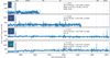 |
Fig. A.1. Spectra extracted from circular apertures (r = 0.6″) centred on the sources shown in the insets. The vertical blue lines mark the emission lines; in the last panel, Balmer and CaII absorption features around 3800 Å are marked with red lines. For each target, we report the spectroscopic redshift, the coordinates, and, for the sources in the DECaLS Survey (Dey et al. 2018), the optical magnitudes. The insets show the [OII] emission maps (with an FOV of 8″ × 8″). |
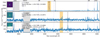 |
Fig. A.2. Spectra extracted from circular apertures (r = 0.6″) centred on the sources shown in the top-left insets. The shaded orange regions highlight the Hα+[N II] system associated with Arp220; the grey regions mark the channels with strong contamination caused by Na lasers. The vertical blue lines mark the brightest emission lines; in the bottom panel, Balmer and CaII absorption features around 3800 Å are marked with red lines. For each source, we report the spectroscopic redshift, the coordinates, and, for the sources in the DECaLS Survey (Dey et al. 2018), the optical magnitudes. The insets show the [O III] (for the first source) and [OII] emission maps for each source. |
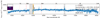 |
Fig. A.3. Spectrum extracted from a circular aperture with (r = 0.6″) centred on the source shown in the top-left insets. Stellar and ISM absorption features are indicated with red lines. The shaded orange region highlights the Na ID system associated with Arp220; the grey regions mark the channels with strong contamination caused by Na lasers. The inset shows the continuum emission at ≈5300 Å. |
The sources at the highest redshifts (z ≈ 1) are shown in the first figure. They can be clearly identified thanks to the bright [OII] doublet at 3729 Å and a few additional fainter emission lines. For the source id1641 (bottom panel), we also identified several stellar absorption features. For id1679 (top panel), only a single emission line is detected; it shows a broad (FWHM ∼ 400 km s−1) and double peaked profile (with a separation of ≈200 km s−1). We also report a tentative detection of a faint feature at ∼8891 Å (with ∼2σ significance). Assuming that the strong feature is the [OII] doublet, the faint feature can be associated with [NeIII]λ3869 emission. We therefore provided a tentative spectroscopic redshift z = 1.2979 for this target.
Gal. III and ID 1641 (third and fourth panels) are at the same redshift, z ≈ 0.7278, and are separated by 7.6″ (∼60 kpc). The different [O III]/[OII] line ratios suggest a different degree of ionisation in the two systems, with Gal. III associated with a higher ionisation state. This is also suggested by the different [O III]/Hβ ratios.
In Fig. A.2 we report the spectra of the three sources at z ≈ 0.5. We clearly identified several emission lines for each of them. Gal. II shows strong [O III] doublet lines, as well as faint Hβ, Hγ, Hδ, and [NeIII]; the high [O III]/Hβ flux ratio could suggest the presence of an AGN in this target. ID 1644 and Gal. I are at the same redshift, z = 0.4993, and are separated by ∼6″ (∼35 kpc). The [O III]/[OII] line ratios are consistent within the errors and are compatible with those of SDSS galaxies (Kauffmann et al. 2003b); the [O III]/Hβ ratio cannot be constrained, due to the presence of bad sky-subtraction residuals around 4861 Å.
In Fig. A.3 we report the spectrum of the nearest source, ID 2070, at z = 0.0901. It shows several stellar features in absorption in addition to the Na ID absorption transitions related to foreground cold gas associated with the Arp220 system. Its spectroscopic redshift has been derived with pPXF, following the same prescriptions introduced in Sect. 4. For all other targets, spectroscopic redshifts are derived by fitting individual emission lines with Gaussian profiles, following the prescriptions presented in Sect. 4.
Appendix B: Monte Carlo analysis for measurement errors on σ*
Figure B.1 shows the mean (left) and the standard error (right) of the σ* measurements obtained from MC trials in the vicinity of the ring-like feature close to the two nuclei. Spectra extracted from six different Voronoi bins are also reported in the insets to show the quality of the data and the pPXF best-fit models.
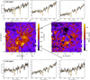 |
Fig. B.1. Mean (left) and the standard error (right) of the σ* measurements obtained from MC trials in the vicinity of the ring-like feature close to the two Arp220 nuclei. Spectra extracted from six different Voronoi bins (labelled with cyan + symbols) are also reported in the insets: Black (orange) curves indicate the spectra (pPXF best-fit models), while vertical green lines mark the position of the CaII triplet lines. |
Appendix C: Emission line decomposition
Figure C.1 show the 2 × 2 pixel spectra with a clear distinction between different kinematic components in the emission line profiles. Their spatial location in the MUSE FOV is shown in Fig. C.2, together with the extent of the associated regions.
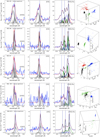 |
Fig. C.1. continued. |
 |
Fig. C.2. Arp220 W80 map showing, with red squares, the location of the 2 × 2 pixel spectra reported in Fig. C.1. The spatial extent of the associated regions with well-determined kinematics are sketched with black squares. |
Appendix D: Balmer lines and [O III]λ5007 best-fit maps
In Fig. D.1 we show the multi-component fit results for the Hβ, [O III]λ5007, Hα, to be compared with the [N II]λ6583 maps in Fig. 10. The Hα maps are very similar to those of [N II]. The main differences are found in the proximity of the SCs at ∼7″ from the Arp220 nuclei, associated with brighter Hα fluxes and narrower Balmer W80. On the contrary, [O III] and Hβ are noisier and their distributions are fuzzy because of the lower S/N; nonetheless, these faint features reveal the same kinematic structures observed in [N II] maps.
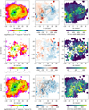 |
Fig. D.1. Hα (top), Hβ (centre), and [O III]λ5007 (bottom) multi-component fit results. See Fig. 10 for details. |
Appendix E: Shock diagnostics and σ[NII] − Vs relation
Figure E.1 shows the correlation between velocity dispersion and emission line ratios as well as the comparison with shock model predictions from MAPPING V assuming a one-to-one relation between σ[NII] and Vs. With this assumption, shock model predictions match the measurements in the [S II] and [O I] diagrams well, at least for the regions with σ[NII] > 200 km s−1. However, they (i) significantly under-predict [N II]/Hα ratios by a factor of ∼0.2 dex, and (ii) do not explain the presence of gas with velocity dispersion < 200 km s−1 and [N II]/Hα, [S II]/Hα, and [O I]/Hα emission line ratios not compatible with SF ionisation. Taking into account these two arguments, we considered the assumption of a one-to-one W80 − Vs relation as more reliable (see Fig. 16).
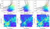 |
Fig. E.1. Top panels: σ[NII] against log([N II]/)Hα, log([S II]/)Hα, and log([O I]/)Hα, from left to right, obtained from the fitted total line profiles. The plotted measurements are colour-coded from purple to red, going from low to high flux ratios and line widths. Dashed and solid lines represent shock model grids from MAPPING V (Sutherland & Dopita 2017; Sutherland et al. 2018; see Fig. 16 for details). We assumed a one-to-one correlation between Vs and σ. For comparison, we also display the shock model predictions derived by Ho et al. (2014, dot-dashed red lines) and by Rich et al. (2011, magenta and purple curves, considering an 80% shock fraction); none of these predictions, derived assuming a pre-shock density of 10 cm−3 and different metallicities and magnetic field strengths (see Sect. 6.2.1 in Ho et al. 2014 and Sect. 7.1 in Rich et al. 2011 for details), match the majority of the Arp220 measurements. Bottom panels: Arp220 maps associated with the top panel diagrams, using the same colour codes. |
Appendix F: Star-formation clumps
In Fig. F.1 we report the integrated spectra of the four SCs identified in the MUSE FOV. All but SC1 show strong [N II] emission and Na ID absorption with asymmetric and broad profiles. This finding is consistent with the fact that such SCs are located very close to – or along – the outflow path (see e.g. Fig. 20).
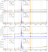 |
Fig. F.1. Integrated spectra of the four SCs identified in the MUSE FOV (black curves). The corresponding pPXF best-fit model profiles are shown with orange curves. The pure emission and absorption ISM spectra (blue curves) are obtained by subtracting the best-fit stellar contribution from the original spectra. The insets show the spectra and stellar models around Na ID and the Hα+[N II] complex. The vertical blue lines mark the wavelengths of the emission lines detected in the spectra; the green lines mark the position of the stellar absorption systems (from left to right: MgI triplet, Na ID and KI doublets, and CaII triplet); in the two insets, dash-dotted magenta lines indicate the median stellar velocity in individual SCs. The regions excluded from the pPXF fits and corresponding to the most intense sky line residuals are highlighted as shaded orange areas; the portion of the spectra around 5700 Å is missing because of a filter blocking the laser contamination. |
All Tables
All Figures
|
Fig. 1. Three-colour optical image of Arp220 obtained by combining HST observations performed through three different filters (B, B+I, and I). The white box indicates the region analysed in this work, corresponding to the MUSE FOV. North is up. Credit: NASA, ESA, the Hubble Heritage Team (STScI/AURA)-ESA/Hubble Collaboration, and A. Evans (University of Virginia, Charlottesville/NRAO/Stony Brook University). |
| In the text | |
|
Fig. 2. Upper left: continuum emission from MUSE data cube, having collapsed the data cube in the range 8025 − 8125 Å (rest frame). A few bright Arp220 clumps (c1 and c2) and background galaxies are labelled (see Appendix A and Table 1); these knots are used to perform a bona fide astrometric registration of the MUSE data (see Sect. 3.2). Upper right: HST/WFC3 F160W image from HST archive (total exposure time of 172 s and pixel scale of 0.13″; PI: Larson). The image shows the region analysed in this work; the white box indicates the portion displayed in the bottom-right panel. Bottom left: zoomed-in insets of 7″ × 7″ showing the continuum emission map around some of the sources selected in the upper-left panel. The overlaid cyan contours represent the NIR emission from the HST image. For the sources in the DECaLS DR7 catalogue (Dey et al. 2018), we mark the DECaLS positions with black crosses. Bottom right: [S III]λ9069 image obtained integrating the flux in the wavelength range 9065 − 9083 Å, after subtracting the continuum emission, with overlaid contours of the NIR emission (upper-right panel). Crosses mark the [S III] nuclear peaks; white circles mark the position of two SCs identified in this work (see Sect. 6). North is up. |
| In the text | |
|
Fig. 3. Arp220 stellar kinematic maps from our pPXF analysis. The contours in the left-hand panel show the negative (dark blue) and positive (dark red) isovelocity curves, from −100 to +100 km s−1, equally spaced in steps of 20 km s−1; the contours in the right-hand panel are derived from the continuum emission image shown in Fig. 2 (top left) and are equally spaced in steps of 0.25 dex, starting from 1.3 × 10⁻¹⁶ erg s−1 cm−2 arcsec−2. The crosses mark the two nuclei; the dashed yellow line in the left-hand panel shows PA = 48°, corresponding to the major axis of Arp220. Right-hand panel: the inset shows a zoomed-in view of the innermost nuclear regions, highlighting the ring-like shape with high σ* values (using a slightly different colour bar); the positions of the two nuclei are shown with black crosses. Stellar velocity dispersions are not corrected for the instrumental broadening. North is up. |
| In the text | |
|
Fig. 4. E (top panel) and W (bottom) nucleus spectra (black curves) extracted from 2 × 2 pixel regions. The corresponding pPXF best-fit model profiles are shown with orange curves. The pure emission and absorption ISM spectra (blue curves) are obtained by subtracting the best-fit stellar contribution from the original spectra. The insets show the spectra and stellar models around Na ID and the Hα+[N II] complex. The vertical blue lines mark the wavelengths of the emission lines detected in the two spectra; the green lines mark the position of stellar absorption systems (from left to right: MgI triplet, Na ID and KI doublets, CaII triplet). The regions excluded from the pPXF fits, and corresponding to the most intense sky line residuals, are highlighted as shaded orange areas; the portion of the spectra around 5700 Å is missing because of a filter blocking the laser contamination. |
| In the text | |
|
Fig. 5. Hα and [N II]λ6583 channel maps obtained by collapsing the ISM data cube on the emission line core (i.e. velocity channels within [−150, +150] km s−1 from the systemic). Contours in the left-hand panel are derived from the continuum emission image shown in Fig. 3, top left; contours in the right-hand panel show the 0.5 − 8 keV emission from Chandra-ACIS observations (OBSID 16092; Paggi et al. 2017). |
| In the text | |
|
Fig. 6. Left: [N II] integrated flux obtained from single Gaussian fits. The first solid contour is 3 × 10⁻¹⁷ erg s−1 cm−2 arcsec−2, and the jump is 0.5 dex. Centre and right: velocity and FWHM maps obtained from single component fits. The solid contours are from the left-hand panel. The crosses mark the two nuclei. |
| In the text | |
|
Fig. 7. Illustration of the profile decomposition method. Top: first three panels show the spectra in the vicinity of the [O III] (left), [O I]λ6300 (centre), and [N II]+Hα lines (right). The red curves represent the best-fit models obtained from 500 MC trials. For all but the [N II]λ6583 and Hα lines, we show the Gaussian profiles used to reproduce the spectrum with grey curves. Different colours are used for the Hα and [N II]λ6583 lines to distinguish the different kinematic components. Dashed grey and blue lines mark the Arp220 systemic and the local stellar velocity, respectively. Right-hand panel: parameter space V − FWHM–[N II]/Hα for the same kinematic components, highlighting the clear separation between the four Gaussian sets. Bottom: best-fit results for one of the nearby Voronoi bins, obtained with the kinematic constraints from the 2 × 2 spectra shown in the top panels. Bottom-right panel: velocity dispersion map with the Voronoi bins (black outlines) associated with the above-defined kinematic constraints; the black (red) contours mark the spaxels from which the top (bottom) spectra have been extracted. |
| In the text | |
|
Fig. 8. Illustration of the profile decomposition method. See Fig. 7 for details. In this region, the velocities of the blue and green Gaussian sets overlap; a clear separation between the two is, however, assured thanks to their distinct FWHMs. |
| In the text | |
|
Fig. 9. Best-fitting models for eight representative spectra in the vicinity of the Na ID complex. The original spectra are shown in black and the pPXF best-fit models in orange; the red profiles represent the best-fit models obtained with the simultaneous multi-component approach. Green, grey, and blue profiles are obtained from Eq. (1) and represent the different kinematic components used to model the Na ID absorption; in the last four panels, the Na ID emission line contribution (modelled with Gaussian profiles) is shown with an arbitrary offset in the y-axis. |
| In the text | |
|
Fig. 10. [N II] multi-component fit results. Left: integrated flux; the first solid contour is 3 × 10⁻¹⁷ erg s−1 cm−2 arcsec−2, and the jump is 0.5 dex. Centre: [N II] velocity (v50) map. Right: [N II] line width (W80) map. The solid contours are from the left-hand panel. The crosses mark the two nuclei. |
| In the text | |
|
Fig. 11. Na ID emission line maps from the multi-component fit. Left: EW. Centre: Na ID velocity (v50) map. Right: Na ID line width (W80) map. The solid contours and crosses are from Fig. 10. |
| In the text | |
|
Fig. 12. Na ID absorption line maps from the multi-component fit. Left: EW. Centre: Na ID velocity (v50) map. Right: Na ID line width (W80) map. The solid contours and crosses are from Fig. 10. |
| In the text | |
|
Fig. 13. Position-velocity diagram, with positions varying along PA = 48° (top) and PA = 138° (bottom) for the stellar component, [N II] gas, and Na ID gas, as labelled in the figure. Distances on the x-axis are measured from the intermediate position between the two nuclei, from the bottom to the top of the FOV. Stellar and gas velocity measurements are obtained by averaging 3 × 3 pixels along a given PA from the maps shown in Figs. 3, 10–12; CO(2–1) velocities are obtained from Fig. 5 in Scoville et al. (1997). |
| In the text | |
|
Fig. 14. Arp220 resolved-BPT diagrams. Left-hand panels: we report the [N II]-BPT (upper), [S II]-BPT (centre), and [O I]-BPT (bottom) diagrams for each Voronoi bin with S/N > 3 in each line. Black curves separate AGN-, SF-, and LI(N)ER-like line ratios (see text for details). For each diagnostic, a map marking each Voronoi bin with the colour corresponding to increasing flux ratios is shown on the right. The colour codes are defined using the ELR functions described in the text. Grey points correspond to [O III]/Hβ lower limits; light-to-dark grey colours in the maps correspond to increasing [N II]/Hα (top right), [S II]/Hα (middle), and [O I]/Hα (bottom) ratios. The contours of [N II] line emission are over-plotted in black. Most of the gas emission is dominated by LI(N)ER-like ionisation. In the [S II]-BPT map, we labelled the position of the four SCs identified in this work. |
| In the text | |
|
Fig. 15. Arp220 map of the [S III]λλ9069, 9532/[S II]λλ6716, 31 ratios, obtained from the fitted total line profiles. Emission line fluxes have been corrected for extinction (see Sect. 8). The contours of [N II] line emission and the position of the E and W nuclei are over-plotted in black. |
| In the text | |
|
Fig. 16. Top panels: W80[NII] against log([N II]/)Hα, log([S II]/)Hα, and log([O I]/)Hα, from left to right, obtained from the fitted total line profiles. The plotted measurements are colour-coded from purple to red, going from low to high flux ratios and line widths. Dashed and solid lines represent shock model grids from MAPPING V (Sutherland & Dopita 2017; Sutherland et al. 2018). Each line connects predicted line ratios of a certain metallicity (1 Z⊙, solid lines; 2 Z⊙, dashed lines), pre-shock electron density (1 cm−3), and magnetic field (from 1 to 10 μG, as labelled in the first panel for 2-Z⊙ models), with changing shock velocities Vs in the range 200 − 1000 km s−1. We assumed a one-to-one correlation between Vs and W80. Bottom panels: Arp220 maps associated with the top panel diagrams, using the same colour codes. |
| In the text | |
|
Fig. 17. Left: Balmer decrement measurements (purple to red) and lower limits (grey to black) across the MUSE FOV. Hα and Hβ fluxes are derived from the fitted total line profiles; 3σ upper limits for the Hβ flux are used to derive Balmer decrement lower limits. Right: E(B − V)gas map of Arp220, derived from the Hα/Hβ ratios in the top-left panel using the CCM extinction law. |
| In the text | |
|
Fig. 18. Top left: E(B − V)gas as a function of the Na ID EW. The dashed line represents Eq. (4), derived under the assumption that both quantities are proportional to the hydrogen column density NH. Top right: covering factor vs. optical depth for each kinematic component used to model the Na ID profiles. The points in the top panels are colour-coded according to their position in the [N II]-BPT diagram (Fig. 14, top right). Bottom left: covering factor map, obtained from the total Na ID profiles following the Rupke et al. (2005a) prescription. Bottom right: column density map, obtained by summing the NH derived from each kinematic component required to model Na ID profiles. |
| In the text | |
|
Fig. 19. [N II] velocity channels extracted from the data cubes containing the best-fit profiles of shock (top) and SF-ionised (bottom) gas. Letters from A to J locate the main kinematic structures discussed in Sect. 10; in the bottom panels, we also mark the position of the four SCs. |
| In the text | |
|
Fig. 20. Schematic view of the main structures in Arp220, revealed by MUSE. The three-colour image shows the [N II] shock emission, reconstructed from multi-component best-fit results. Superimposed yellow lines highlight the biconical outflow. Star symbols identify the four main SCs identified in Sect. 10. Cyan curves locate the main dust filaments possibly affecting the outflow geometry. The same curves are reported in the inset, showing the blue stellar continuum emission as well as the dusty structures in the innermost nuclear regions of Arp220. |
| In the text | |
|
Fig. 21. Distribution of gas ionised by young and massive stars, traced by Hα emission. All fluxes have been corrected for dust attenuation. See Sect. 11 for details. |
| In the text | |
|
Fig. A.1. Spectra extracted from circular apertures (r = 0.6″) centred on the sources shown in the insets. The vertical blue lines mark the emission lines; in the last panel, Balmer and CaII absorption features around 3800 Å are marked with red lines. For each target, we report the spectroscopic redshift, the coordinates, and, for the sources in the DECaLS Survey (Dey et al. 2018), the optical magnitudes. The insets show the [OII] emission maps (with an FOV of 8″ × 8″). |
| In the text | |
|
Fig. A.2. Spectra extracted from circular apertures (r = 0.6″) centred on the sources shown in the top-left insets. The shaded orange regions highlight the Hα+[N II] system associated with Arp220; the grey regions mark the channels with strong contamination caused by Na lasers. The vertical blue lines mark the brightest emission lines; in the bottom panel, Balmer and CaII absorption features around 3800 Å are marked with red lines. For each source, we report the spectroscopic redshift, the coordinates, and, for the sources in the DECaLS Survey (Dey et al. 2018), the optical magnitudes. The insets show the [O III] (for the first source) and [OII] emission maps for each source. |
| In the text | |
|
Fig. A.3. Spectrum extracted from a circular aperture with (r = 0.6″) centred on the source shown in the top-left insets. Stellar and ISM absorption features are indicated with red lines. The shaded orange region highlights the Na ID system associated with Arp220; the grey regions mark the channels with strong contamination caused by Na lasers. The inset shows the continuum emission at ≈5300 Å. |
| In the text | |
|
Fig. B.1. Mean (left) and the standard error (right) of the σ* measurements obtained from MC trials in the vicinity of the ring-like feature close to the two Arp220 nuclei. Spectra extracted from six different Voronoi bins (labelled with cyan + symbols) are also reported in the insets: Black (orange) curves indicate the spectra (pPXF best-fit models), while vertical green lines mark the position of the CaII triplet lines. |
| In the text | |
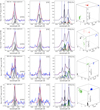 |
Fig. C.1. Illustration of the profile decomposition method. See Fig. 7 for details. |
| In the text | |
|
Fig. C.1. continued. |
| In the text | |
|
Fig. C.2. Arp220 W80 map showing, with red squares, the location of the 2 × 2 pixel spectra reported in Fig. C.1. The spatial extent of the associated regions with well-determined kinematics are sketched with black squares. |
| In the text | |
|
Fig. D.1. Hα (top), Hβ (centre), and [O III]λ5007 (bottom) multi-component fit results. See Fig. 10 for details. |
| In the text | |
|
Fig. E.1. Top panels: σ[NII] against log([N II]/)Hα, log([S II]/)Hα, and log([O I]/)Hα, from left to right, obtained from the fitted total line profiles. The plotted measurements are colour-coded from purple to red, going from low to high flux ratios and line widths. Dashed and solid lines represent shock model grids from MAPPING V (Sutherland & Dopita 2017; Sutherland et al. 2018; see Fig. 16 for details). We assumed a one-to-one correlation between Vs and σ. For comparison, we also display the shock model predictions derived by Ho et al. (2014, dot-dashed red lines) and by Rich et al. (2011, magenta and purple curves, considering an 80% shock fraction); none of these predictions, derived assuming a pre-shock density of 10 cm−3 and different metallicities and magnetic field strengths (see Sect. 6.2.1 in Ho et al. 2014 and Sect. 7.1 in Rich et al. 2011 for details), match the majority of the Arp220 measurements. Bottom panels: Arp220 maps associated with the top panel diagrams, using the same colour codes. |
| In the text | |
|
Fig. F.1. Integrated spectra of the four SCs identified in the MUSE FOV (black curves). The corresponding pPXF best-fit model profiles are shown with orange curves. The pure emission and absorption ISM spectra (blue curves) are obtained by subtracting the best-fit stellar contribution from the original spectra. The insets show the spectra and stellar models around Na ID and the Hα+[N II] complex. The vertical blue lines mark the wavelengths of the emission lines detected in the spectra; the green lines mark the position of the stellar absorption systems (from left to right: MgI triplet, Na ID and KI doublets, and CaII triplet); in the two insets, dash-dotted magenta lines indicate the median stellar velocity in individual SCs. The regions excluded from the pPXF fits and corresponding to the most intense sky line residuals are highlighted as shaded orange areas; the portion of the spectra around 5700 Å is missing because of a filter blocking the laser contamination. |
| In the text | |
Current usage metrics show cumulative count of Article Views (full-text article views including HTML views, PDF and ePub downloads, according to the available data) and Abstracts Views on Vision4Press platform.
Data correspond to usage on the plateform after 2015. The current usage metrics is available 48-96 hours after online publication and is updated daily on week days.
Initial download of the metrics may take a while.