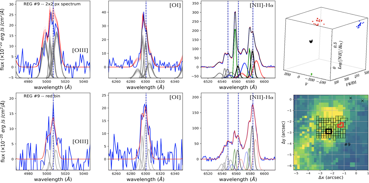
Illustration of the profile decomposition method. Top: first three panels show the spectra in the vicinity of the [O III] (left), [O I]λ6300 (centre), and [N II]+Hα lines (right). The red curves represent the best-fit models obtained from 500 MC trials. For all but the [N II]λ6583 and Hα lines, we show the Gaussian profiles used to reproduce the spectrum with grey curves. Different colours are used for the Hα and [N II]λ6583 lines to distinguish the different kinematic components. Dashed grey and blue lines mark the Arp220 systemic and the local stellar velocity, respectively. Right-hand panel: parameter space V − FWHM–[N II]/Hα for the same kinematic components, highlighting the clear separation between the four Gaussian sets. Bottom: best-fit results for one of the nearby Voronoi bins, obtained with the kinematic constraints from the 2 × 2 spectra shown in the top panels. Bottom-right panel: velocity dispersion map with the Voronoi bins (black outlines) associated with the above-defined kinematic constraints; the black (red) contours mark the spaxels from which the top (bottom) spectra have been extracted.