| Issue |
A&A
Volume 602, June 2017
|
|
|---|---|---|
| Article Number | A68 | |
| Number of page(s) | 25 | |
| Section | Extragalactic astronomy | |
| DOI | https://doi.org/10.1051/0004-6361/201629009 | |
| Published online | 14 June 2017 | |
Molecular gas, dust, and star formation in galaxies
I. Dust properties and scalings in ~1600 nearby galaxies
1 Department of Astronomy, Universidad de Concepción, Casilla 160-C Concepción, Chile
e-mail: This email address is being protected from spambots. You need JavaScript enabled to view it.
, This email address is being protected from spambots. You need JavaScript enabled to view it.
2 Instituto de Física y Astronomía, Universidad de Valparaíso, Avda. Gran Bretaña 1111, Valparaíso, Chile
3 Laboratoire AIM-Paris-Saclay, CEA/DSM/Irfu – CNRS – Université Paris Diderot, Saclay, pt courrier 131, 91191 Gif-sur-Yvette, France
4 Argelander-Institut für Astronomie, Universität Bonn, Auf dem Hügel 71, 53121 Bonn, Germany
5 Joint ALMA Observatory, Alonso de Córdova 3107, Vitacura 763-0355, Santiago, Chile
6 European Southern Observatory, Alonso de Córdova 3107, Vitacura, Casilla 19001, 19 Santiago, Chile
7 Departamento de Ciencias Fisicas, Universidad Andres Bello, Sede Concepcion, autopista Concepcion-Talcahuano 7100, Talcahuano, Chile
Received: 25 May 2016
Accepted: 28 March 2017
Abstract
Context. Dust and its emission is increasingly being used to constrain the evolutionary stage of a galaxy. A comprehensive characterization of dust, best achieved in nearby bright galaxies, is thus a highly useful resource.
Aims. We aim to characterize the relationship between dust properties (mass, luminosity, and temperature) and their relationships with galaxy-wide properties (stellar, atomic, and molecular gas mass, and star formation mode). We also aim to provide equations to accurately estimate dust properties from limited observational datasets.
Methods. We assemble a sample of 1630 nearby (z < 0.1) galaxies – over a large range of stellar masses (M∗), star formation rates (SFR) and specific star formation rates (sSFR = SFR/M∗) – for which comprehensive and uniform multi-wavelength observations are available from WISE, IRAS, Planck, and/or SCUBA. The characterization of dust emission comes from spectral energy distribution (SED) fitting using Draine & Li (2007, ApJ, 657, 810) dust models, which we parametrize using two components (warm at 45–70 K and cold at 18–31 K). The subsample of these galaxies with global measurements of CO and/or HI are used to explore the molecular and/or atomic gas content of the galaxies.
Results. The total infrared luminosity (LIR), dust mass (Mdust), and dust temperature of the cold component (Tcold) form a plane that we refer to as the dust plane. A galaxy’s sSFR drives its position on the dust plane: starburst (high sSFR) galaxies show higher LIR , Mdust , and Tcold compared to main sequence (typical sSFR) and passive galaxies (low sSFR). Starburst galaxies also show higher specific dust masses (Mdust/M∗) and specific gas masses (Mgas/M∗). We confirm earlier findings of an anti-correlation between the dust to stellar mass ratio and M∗ . We also find different anti-correlations depending on sSFR; the anti-correlation becomes stronger as the sSFR increases, with the spread due to different cold dust temperatures. The dust mass is more closely correlated with the total gas mass (atomic plus molecular) than with the individual atomic and molecular gas masses. Our comprehensive multiwavelength data allows us to define several equations to accurately estimate LIR , Mdust , and Tcold from one or two monochromatic luminosities in the infrared and/or sub-millimeter.
Conclusions. It is possible to estimate the dust mass and infrared luminosity from a single monochromatic luminosity within the Rayleigh-Jeans tail of the dust emission, with errors of 0.12 and 0.20 dex, respectively. These errors are reduced to 0.05 and 0.10 dex, respectively, if the dust temperature of the cold component is used. The dust mass is better correlated with the total ISM mass (MISM ∝Mdust0.7). For galaxies with stellar masses 8.5 < log(M∗/M⊙) < 11.9, the conversion factor between the single monochromatic luminosity at 850 μm and the total ISM mass (α850 μm) shows a large scatter (rms = 0.29 dex) and a weak correlation with the LIR . The star formation mode of a galaxy shows a correlation with both the gas mass and dust mass: the dustiest (high Mdust /M∗) galaxies are gas-rich and show the highest SFRs.
Key words: galaxies: ISM / galaxies: photometry / galaxies: star formation / infrared: ISM / submillimeter: galaxies
© ESO, 2017
1. Introduction
Star formation occurs within dense (n(H2) ~ 102−105 cm-3), massive (104−106M⊙), and cold (Tgas ~ 10–50 K) giant (10 ~ 100 pc) molecular clouds (GMC; Kennicutt & Evans 2012), where atomic gas, mainly atomic Hydrogen (HI), is transformed into molecular gas (mainly H2) on dust grain surfaces (e.g., Scoville 2013). Dust grains are formed within the cool, extended atmospheres of low-mass (1–4 M⊙) asymptotic giant branch (AGB) stars and are dispersed into the ISM via the strong AGB star winds (Gehrz 1989). In other words, the dust content is related to the star formation history of the galaxy. Since much of our current knowledge of galaxy properties and evolution comes from studies of high-temperature (T > 103 K) regions, a global understanding of star formation requires a better knowledge of the role of cold gas and dust in the star formation process.
Dust grains emit mainly in the far infrared (FIR; 40 <λ< 300 μm) and sub-millimeter (sub-mm; 300 <λ< 1000 μm). Early studies of dust content and emission have been done both from space (IRAS, see Neugebauer et al. 1984 and ISO; see Kessler et al. 1996) and from the ground (SCUBA, see Holland et al. 1999, at the James Clerk Maxwell Telescope and MAMBO at the IRAM 30 m telescope). More recent missions – in the mid-infrared (e.g., WISE; Spitzer), far-infrared (e.g., AKARI; Herschel), and sub-mm (e.g., Planck) – have revolutionized the field (e.g., Lutz 2014).
The IR to sub-mm emission of dust has been characterized in many samples (e.g., SLUGs by Dunne et al. 2000; HRS by Boselli et al. 2010; KINGFISH/SINGS by Kennicutt et al. 2003; Dale et al. 2005; SDSS-IRAS by da Cunha et al. 2010; ATLAS 3D by Cappellari et al. 2011; ERCSC by Negrello et al. 2013) and at high-z (e.g., GOODS-Herschel by Magnelli et al. 2010; H-ATLAS by Eales et al. 2010). Early studies modeled the dust grain emission using gray-body emission from one or two dust-temperature components (e.g., Dunne et al. 2000; Dunne & Eales 2001). More complex and sophisticated dust-emission models available today include the MAGPHYS (da Cunha et al. 2010) code, which contains empirically-derived spectral energy density (SED) libraries from the ultraviolet (UV) to infrared (IR), and the model developed by Draine & Li (2007, DL07 hereafter), which provides a more extensive SED library covering the IR to sub-mm. The DL07 model has been successfully applied to the Spitzer Nearby Galaxy Survey (SINGS) galaxies (Draine et al. 2007), and these authors note that the presence of sub-mm photometry is crucial to constrain the mass of the cold dust component.
The results on dust properties coming from many of the studies mentioned above are limited by poor statistics as a consequence of small samples and/or the limited sampling of the SED (especially at sub-mm wavelengths), which decreases the reliability of the SED modeling. Since dust properties are increasingly used at all redshifts to determine the evolutionary state of a galaxy, and in general for galaxy evolution studies, it is crucial to fully characterize these properties and their relationships and degeneracies in large samples of galaxies. Of specific interest is the degeneracy between dust temperatures and dust emissivity index, the inter-relationships between dust mass, temperature, and luminosity, and the relationships between these dust properties and other properties of the galaxy (e.g., stellar and gas masses, SFR, specific star formation rate; sSFR = SFR/M∗[yr-1]).
The recent availability of Planck sub-mm (350 μm to 850 μm) fluxes for thousands of nearby galaxies which are well studied in the optical to IR, allows, for the first time, comprehensive and accurate dust model fits to these. With a comprehensively modeled large sample of nearby galaxies in hand, one can test and refine the many scaling relations and estimators now being used at all redshifts, for example, estimating gas mass from a single flux measurement at 850 μm (Scoville 2013), or estimating dust masses (Dunne et al. 2000; Dunne & Eales 2001) and/or luminosities (e.g., Sanders & Mirabel 1996; Elbaz et al. 2010) from a few IR flux measurements.
The “starburstiness” of a galaxy is normally obtained from the ratio of the SFR and the stellar mass (M∗). The SFR –M∗ plane shows that while most “normal” star forming galaxies follow a “main sequence” (MS) of secular star formation (Elbaz et al. 2007), a small fraction of galaxies show excessive SFR for a given M∗ : these galaxies are referred to as starburst (SB). The MS of galaxies is observed over the redshift range z ~ 0–4 (e.g., Elbaz et al. 2007; Magdis et al. 2010; Rodighiero et al. 2011; Elbaz et al. 2011; Pannella et al. 2015; Schreiber et al. 2015) and changes smoothly with redshift (Elbaz et al. 2011). In this work we use the MS proposed by Elbaz et al. (2011), at z = 0: ![Mathematical equation: \begin{equation} SFR=\frac{M_{*}}{4.0\times10^{9}}\left[\frac{\msun}{\rm yr}\right] \label{eq:SFR elbaz} \cdot \end{equation}](/articles/aa/full_html/2017/06/aa29009-16/aa29009-16-eq32.png) (1)This equation defines the specific star formation rate
(1)This equation defines the specific star formation rate ![Mathematical equation: \hbox{$\left(sSFR\rm \ [yr^{-1}] =\it SFR/\mstar\right)$}](/articles/aa/full_html/2017/06/aa29009-16/aa29009-16-eq33.png) expected for MS galaxies (MS; − 0.5 < sSFR [yr-1] < 0.5). We define SB galaxies as those having sSFR [yr-1] > 0.8, and passive (PAS) galaxies as those at sSFR [yr-1] < −0.8. The two “transition” zones between the above three classifications, that is, 0.5 ≤ SFR [M⊙ yr-1] < 0.8 dex with regards to the MS locus (an intermediate SB zone) and; − 0.8 ≤ SFR [M⊙ yr-1] < −0.5 dex with regards to the MS locus (an intermediate passive zone) are excluded in order to avoid contamination.
expected for MS galaxies (MS; − 0.5 < sSFR [yr-1] < 0.5). We define SB galaxies as those having sSFR [yr-1] > 0.8, and passive (PAS) galaxies as those at sSFR [yr-1] < −0.8. The two “transition” zones between the above three classifications, that is, 0.5 ≤ SFR [M⊙ yr-1] < 0.8 dex with regards to the MS locus (an intermediate SB zone) and; − 0.8 ≤ SFR [M⊙ yr-1] < −0.5 dex with regards to the MS locus (an intermediate passive zone) are excluded in order to avoid contamination.
In this paper, we capitalize on the recent availability of sub-mm (Planck) fluxes (for better dust model fits) and WISE fluxes (for stellar mass determinations) to fit DL07 dust models to all nearby bright galaxies for which sufficient (for a reasonable fit to DL07 models) multi-wavelength uniform data are available from WISE, IRAS, Planck, and/or SCUBA. The resulting model fits are used to explore the relationship between dust properties (mass, luminosity, temperature) and their relationship with other galaxy-wide properties (e.g., stellar and gas masses, sSFR). The comprehensive dust modeling also allows us to refine estimations of total IR luminosity from one to a few IR to sub-mm fluxes, the dust mass from a single sub-mm flux, and sSFR from IR to sub-mm colors.
Throughout this paper we adopt a flat cosmology with Ωm = 0.3 and H0 = 72 km s-1 Mpc-1.
2. Samples and data
We use two samples of nearby galaxies: (a) the sample of nearby galaxies with detections in Planck High Frequency Instruments (HFI) Second Data Release catalog and global CO J:1-0 observations (Nagar et al., in prep.); and (b) all galaxies from the 2MASS Redshift Survey (2MRS; Huchra et al. 2012), which are listed as detections in the second Planck Catalog of Compact Sources at 350 μm, 550 μm, and 850 μm (PCCS2; Planck Collaboration XXVII 2016).
The Nagar et al. (in prep.) sample is a compilation of approximately 600 nearby galaxies (⟨ z ⟩ = 0.06) with global CO J:1-0 observations, and sub-mm fluxes from Planck catalogs at 350 μm, 550 μm, and 850 μm or SCUBA 850 μm observations. The names of the catalogs with the respective references are summarized in Table 1.
Source samples in the Nagar et al. compilation.
The sample spans a range of morphological types – including spiral, elliptical and interacting galaxies – and luminosities from normal to Ultra-Luminous Infrared Galaxies (ULIRGs).
The 2MRS sample consists of 44,599 nearby (⟨ z ⟩ = 0.03) 2MASS (Shectman et al. 1996) galaxies with Ks ≥ 11.75 mag and Galactic latitude | b | ≥ 5 for which spectroscopic redshifts have been obtained to 97.6% completeness (Huchra et al. 2012). We matched the 2MRS sample with the (PCCS2), using a maximum matching radius of 1 arcmin. The PCCS2 catalog contains only galaxies with high reliabilities (>80%; signal to noise >5 in DETFLUX). Sources with lower or unknown reliabilities are listed in the equivalent excluded catalog (PCCS2E), which we have not used.
The Planck satellite has a beam resolution of the order of 1 arcmin (e.g., 4.22 arcmin at 350 μm, Planck Collaboration XXVII 2016), and the reliability catalog contains approximately 1000 sources (e.g., 4891 galaxies at 350 μm, Planck Collaboration XXVII 2016), with a density <1 sources/deg2 (e.g., 0.26 sources/deg2 at 350 μm, Planck Collaboration XXVII 2016). This means that the resolutions of WISE and 2MASS (~1 arcsec) do not represent a problem for the match with the Planck source catalog, as we adopt a search radius of 1.0 arcmin. In order to remove any multiple matches, we performed a visual inspection of all the matched objects. In some cases, we selected all the galaxies that have companions in the WISE, 2MASS, and SDSS images and classified them as interacting systems. Furthermore, multiple detections in one Planck beam do not represent a problem either because the galaxies in our sample have a median diameter (parametrized as the D25 reported in HyperLeda1) of 1.5 arcmin, with only 291 having D25 < 1.0 arcmin (~18% of the final sample).
2.1. Flux densities and derived stellar mass
The Planck collaboration (Planck Collaboration XXVII 2016) showed that, at 350 μm, for sources with APERFLUX > 1.0 Jy, the APERFLUXes reported in the Planck catalog are in agreement with those in the Herschel Reference Survey.
Nagar et al. (in prep.) compare the Planck observations at 850 μm with SCUBA data (at 850 μm) in nearby galaxies, revealing that the APERFLUX and the DETFLUX from Planck show the existence of some systematic difference. However, Nagar et al. (in prep.) also show that simple corrections can solve this problem. They find that the observation of fluxes smaller than twice the 90% completeness limit (304 mJy at 850 μm) needs smaller corrections if the DETFLUX is used (the correction is fPlanck 850 μm = fSCUBA 850 μm+70), and for greater fluxes (greater than twice the 90% completeness limit) the fluxes are more consistent with the APERFLUX (using the correction: fPlanck 850 μm = fSCUBA 850 μm+139). Assuming a gray-body with a temperature of T = 25 K and β = 1.8, Nagar et al. (in prep.) obtain similar corrections for Planck observations at 350 and 550 μm. For each wavelength, Nagar et al. (in prep.) obtain three corrections: one with free slope and intercept, a second with intercept zero and free slope, and a third with with free intercept and fixed slope. We use the last kind of correction in our work. Additionally, to correct for the typical spectral shape of dust gray-body emission, we used correction factors of 0.976, 0.903, and 0.887 at 350 μm, 550 μm and 850 μm, respectively Negrello et al. (2013). Following Nagar et al. (in prep.), we assumed a 3% contamination from the CO emission line at Planck 850 μm and negligible CO emission line contamination at Planck 350 and 550 μm. After these flux density corrections are applied, the limits obtained for the Planck-derived flux densities in our sample are 500 mJy, 315 mJy, and 175 mJy, at 350 μm, 550 μm, and 850 μm, respectively.
Mid-infrared (MIR) fluxes are obtained from the AllWISE Source Catalog “g” magnitudes2. These “g” magnitudes are calculated over apertures defined using 2MASS images, with additional corrections as described in Jarrett et al. (2013). The WISE (W1-W4) filters have a limiting sensitivity of 0.08, 0.11, 1, and 6 mJy, respectively. We select only sources with signal to noise (S/N) ≥ 5, except for W4, where we consider a S/N ≥ 3. We calculate the galaxy stellar mass (M∗) using the WISE W1 filter (3.4 μm) and the W1-W2 (4.6 μm) color following the Cluver et al. (2014) calibration. The stellar mass ranges between 109 and 1011M⊙ for our sample. To test the consistency of our WISE-estimated stellar masses, we compare our stellar masses to those in three other catalogs based on SDSS-derived quantities (i.e., NASA-Sloan Atlas, Chang et al. 2015, and MPA-JHU catalogs, see Appendix C). We obtained a good agreement with the M∗ obtained in the NASA-Sloan Atlas (see Appendix C for more details).
The infrared (IR) data comes from the Infrared Astronomical Satellite (IRAS) at 12, 25, 60 and 100 μm, obtained from the Galaxies and Quasars catalog (Fullmer & Lonsdale 1989). We consider only sources with moderate- or high- quality fluxes (no upper limits), with signal to noise ≥ 3.
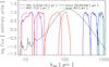 |
Fig. 1 An example dust-emission template from Draine & Li (2007), between 7 and 1100 μm. Overlaid are the transmission curves of all the filters used in this work: WISE W3 and W4 ; IRAS 12, 25, 60 and 100 μm; Planck 350, 550 and 850 μm and SCUBA 850 μm. |
Figure 1 shows the filter band-passes of all filters for which we compiled flux densities which were then used to constrain the DL07 dust model fits: WISE W3 (12 μm) and W4 (22 μm); IRAS 12, 25, 60 and 100 μm; Planck 350, 550 and 850 μm and SCUBA 850 μm. When multiple flux density measurements at the same wavelength are available, we use WISE W3 and W4 in preference to IRAS 12 and 25 μm, and Planck 850 μm in preference to SCUBA 850 μm.
2.2. Gas masses and distances
For the comparison between the dust masses and the ISM content, we require HI data for our galaxies. The integrated flux of HI is obtained from different surveys, detailed in Table 2.
HI surveys used in this work.
The molecular gas mass (Mmol) is calculated from global (non-interferometric) observations of the CO(J: 1-0) line (expressed in terms of the velocity-integrated flux or  [K km s-1 pc2] Solomon et al. 1997 ) and the conversion factor αCO (Solomon & Vanden Bout 2005; Bolatto et al. 2013). The correlation between the galaxy metallicity and the αCO value (Leroy et al. 2011; Sandstrom et al. 2013) shows that the αCO takes values ~ 2 to ~ 20 times the Galactic value for sources with metallicities (12+log(O/H)) smaller than 8.2. In our sample, the stellar mass ranges between 109 and 1011M⊙. Over this stellar mass range, metallicities are expected to be between 8.4 and 9.1 (Tremonti et al. 2004). Over this limited metallicity range, it is valid to use a constant value of αCO (Leroy et al. 2011). In our study, we use αCO = 4.3 [M⊙ (K km s-1 pc
 ] which includes a correction for heavy elements of 36% (Bolatto et al. 2013).
Galaxy distances are derived from the redshift listed in 2MRS or the NASA/IPAC Extragalactic Database (NED)3 except for very nearby galaxies (z< 0.045; DL< 20 Mpc) for which we use distances from the Extragalactic Distance Database (EDD)4.
2.3. AGN contamination
Since our study is focused on dust emission, it is crucial to discard galaxies in which the IR and sub-mm fluxes are highly contaminated by AGN emission. We use the Véron-Cetty & Véron (2010) catalog to identify and discard sources with AGN. This catalog contains 168 941 objects at redshifts between 0 and 6.43 (from which 5569 are at z< 0.1). We discarded all (345) sources in our sample which fall within 30′′ of any source in the Véron-Cetty & Véron (2010) catalog. Additionally, using the AGN selection criteria showed by Cluver et al. (2014) based on WISE colors (using filters W1,W2 and W3), we rejected 43 galaxies. Finally, we excluded all (73) sources with Rayleigh-Jeans (RJ; λ> 300 μm) spectral slope significantly lower than that expected from a gray-body with β = 1.3 and T = 15 K, since for these sources the emission in the RJ regime is likely contaminated by synchrotron emission. In other words, these β and T values imply the exclusion of all sources with colors: f350/f550< 2.3, f350/f850< 6.6 and f550/f850< 2.9 where f350, f550 and f850 are the Planck fluxes at 350, 550 and 850 μm, respectively.
2.4. Final sample
Since our analysis requires accurate fitting of dust model SEDs from IR to sub-mm data, we restrict the two samples above to only those galaxies for which meaningful spectral fits are found (see Sect. 4.1). The final sample – with dust SED fits – comprises 1630 galaxies, which all have reliable M∗ estimations. Of these galaxies, 136 are CO-detected and 1230 have HI masses. From visual inspection of the SDSS and 2MASS images we classified 87 galaxies as interacting in the sample.
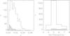 |
Fig. 2 Distribution of redshift (left) and number of photometric points per galaxy (right) for the 1630 objects in our final sample. The shaded histograms in both panels show the equivalent distributions for the subset of galaxies with CO detections. |
The redshift distribution of the final sample is shown in the left panel of Fig. 2. The median redshift is ⟨ z ⟩ = 0.015 for the entire sample, with a mean of 0.012 and sigma = 0.011. For the subsample of galaxies with CO measurements, the median value is ⟨ z ⟩ = 0.0066. with mean of 0.0032 and sigma of 0.0042. The distribution of the number of photometric data points (between 12 μm and 850 μm) per galaxy is shown in the right panel of Fig. 2: 21% of the sample have more than six photometric points, 67% have five, and only 12% have four photometric points. The subsample of galaxies with CO observations has a median of six photometric points per galaxy; 59% of these galaxies have ≥six photometric data points and only 6% have four photometric data points. In all cases we cover both sides of the emission peak at ~100 μm; for the few galaxies with only 5 photometric data points, these are distributed as 2 or 3 points at λ< 100 μm and 1 or 2 at λ> 100 μm.
3. Modeling dust emission
The DL07 model describes the total galaxy spectrum by a linear combination of one stellar component, approximated by a black body with a specific color temperature T∗, and two dust components. One component with dust fraction = (1−γ) is located in the diffuse interstellar medium (ISM) and heated by a radiation field with constant intensity U = Umin; the other component with dust fraction = γ is exposed to a radiation field generated by photo-dissociation regions (PDRs) parametrized by a power-law Uα, over a range of intensities Umin<U<Umax, with Umax ≫ Umin.
Thus, the canonical model emission spectrum of a ga- laxy is: ![Mathematical equation: \begin{equation} \emph{f}_{\nu}^{\rm ~model}=\Omega_{*}B_{\nu}\left(T_{*}\right)+\frac{M_{\rm dust}}{4\pi D_{\rm L}^{2}}\left[\left(1-\gamma\right)p_{\nu}^{(0)}+\gamma p_{\nu}\right] \label{eq:model-flux} , \end{equation}](/articles/aa/full_html/2017/06/aa29009-16/aa29009-16-eq93.png) (2)where Ω∗ is the solid angle subtended by stellar photospheres, Mdust is the dust mass, DL is the luminosity distance, and
(2)where Ω∗ is the solid angle subtended by stellar photospheres, Mdust is the dust mass, DL is the luminosity distance, and  is the emitted power per unit frequency per unit dust mass from dust heated by a single starlight intensity Umin. The dust is a mixture of carbonaceous and amorphous silicate grains characterized by the polycyclic aromatic hydrocarbon (PAH) index, qPAH, defined as the percentage of the total grain mass contributed by PAHs with less than 103 carbon atoms. Finally, pν(qPAH,Umin,Umax,α) is similar to the previous term but for dust heated by a power law distribution of starlight intensities dM/ dU ∝ U− α extending from Umin to Umax. For a known galaxy distance, the canonical dust model is thus characterized by eight free parameters: Ω∗,T∗,qPAH,Umin,Umax,α,γ and Mdust .
The use of all eight free parameters in the DL07 model requires extensive observational datasets and it is computationally demanding. For the former reason, we limit the number and range of the free parameters as follows: (a) we use the Draine & Lee model library (available on the web5). That library uses a limited parameter range for and pν(qPAH,Umin,Umax,α) in Eq. (2); in which qPAH takes 11 values between 0.01 and 4.58, Umin takes 22 values between 0.10 to 25.0 and Umax takes 5 values between 103 to 107 (as a reference, U = 1 corresponds to the starlight intensity estimate for the local ISM) and fixed the value α = 2; (b) we follow Draine et al. (2007), who show that the dust emission of the galaxies of the KINGFISH sample can be well fitted using DL07 models with fixed value of Umax = 106; (c) the stellar component, the first term in Eq. (2), is significant only at λ ≲ 10 μm. Given that we use photometric data at 12 μm ≤ λ ≤ 1000 μm, then we do not require to use this stellar component. To test the influence of the stellar component in fluxes at 12 and 22 μm, we extrapolate the power law obtained from fluxes at 3.4 and 4.6 μm (W1 and W2, respectively), deriving an influence of 4% and 1% at 12 and 22 μm, respectively. This means that the stellar component does not affect our dust emission results. In summary: two parameters (Ω∗ and T∗) are not used since we do not model the stellar component, two parameters (Umax and α) are fixed to a single value, two parameters (qPAH and Umin) are limited in their range, and only Mdust and γ are allowed to vary freely (the Mdust is fixed after the minimization described below in Eq. (4) and γ runs between 0.0 and 100 in steps of 0.1). With these restrictions, we generate 24 200 template SEDs with luminosities per dust mass (νLν/Mdust) in [L⊙/M⊙] and wavelengths (λ) in [μm]. Each observed galaxy SED is fitted to each of the 24 200 SED templates solely by varying Mdust . The best fit value of Mdust is calculated by the minimization of χ2, where  (3)Here
  is the observed flux at the ith band in Jy with an error
  , and
, and  is the DL07 template flux per unit dust mass in units of (Jy /M⊙), convolved with the response function for the ith band.
The minimization of the Eq. (3) gives:![Mathematical equation: \begin{equation} M_{\rm dust}\left[\msun\right]=\suma\left(\sumb\right)^{-1} \label{eq:dustmass} \cdot \end{equation}](/articles/aa/full_html/2017/06/aa29009-16/aa29009-16-eq125.png) (4)The accuracy of the fit is parametrized by the reduced χ2
(4)The accuracy of the fit is parametrized by the reduced χ2 /d.o.f.; d.o.f. = degrees of freedom) value.
For this best fit value of Mdust (and for each of the 24 200 SED templates) we calculate the template spectrum from Eq. (2) and obtain the total infrared [8 to 1000 μm] luminosity (LIR) following: ![Mathematical equation: \begin{equation} L=\int^{\lambda_{\rm max}}_{\lambda_{\rm min}}L_{\nu}\left(\lambda\right)\times\frac{c}{\lambda^2}\left[\lsun\right]~{\rm d}\lambda \label{eq:lum integred} . \end{equation}](/articles/aa/full_html/2017/06/aa29009-16/aa29009-16-eq128.png) (5)Instead of using only the final best fit template for a given galaxy, it is more robust to use a final template fit (FTF) which is the weighted mean of all templates for which
(5)Instead of using only the final best fit template for a given galaxy, it is more robust to use a final template fit (FTF) which is the weighted mean of all templates for which  . Thus, the values of Mdust and LIR are calculated as the geometric mean, weighted by the individual
  , of all templates which satisfy our criteria.
Given that the dust in the DL07 models is distributed in two components (diffuse and PDR, each with a different radiation field intensity) a large range of dust temperatures is present. For several reasons – especially to search for systematic changes with other parameters – it is useful to characterize the dust as having a single, or at most two, temperature(s). We use two methods to characterize the effective temperature(s) of the FTF. We calculate the luminosity weighted temperature (Tweight) of the FTF, defined as: ![Mathematical equation: \begin{equation} T_{\rm weight}{\rm [K]}=\sum_{i=0}^{N}\frac{b}{\lambda_i}~ L_{\lambda,i} \left(\sum_{i=0}^{N} L_{\lambda,i}\right)^{-1} \label{eq:t weighted} , \end{equation}](/articles/aa/full_html/2017/06/aa29009-16/aa29009-16-eq132.png) (6)where b is the Wien’s displacement constant (~2897 [μm K]), and Lλ,i is the monochromatic luminosity at wavelength λi. We also fit a two-temperature dust model to the FTF of the galaxy, using a cold dust component
(6)where b is the Wien’s displacement constant (~2897 [μm K]), and Lλ,i is the monochromatic luminosity at wavelength λi. We also fit a two-temperature dust model to the FTF of the galaxy, using a cold dust component  and a warm dust component
  , each described by a gray-body spectrum:
  (7)where ν is the frequency, A1 and A2 are normalization factors for each gray-body, β is the dust emissivity index (assumed to be the same for both components)6, and B(ν,Tcold) and (B(ν,Twarm) are the Planck functions for the cold and warm dust components, respectively. The fit was performed using the MPFIT code7, which uses a robust minimization routine to obtain the best fit. The two-temperature dust model fits were performed over the wavelength range 22–1000 μm; wavelengths shorter than 22 μm were not used to avoid the complexity of the PAH emission features.
In this work we use dust mass (Mdust) obtained from the DL07 fits, that is, from the FTF. However, for comparison, we also calculate the dust mass implied by the two temperature dust model fit ( ). The total dust mass of the two temperature dust model fit is calculated as follows: (see Dunne & Eales 2001):
 ![Mathematical equation: \begin{equation} M_{\rm dust}^{\rm 2gb}=\frac{S_{850}D_{\rm L}^{2}}{\kappa_{850}}\times\left[\frac{N_{\rm cold}}{B(850,T_{\rm cold})}+\frac{N_{\rm warm}}{B(850,T_{\rm warm})}\right] \label{eq:2gb Md} , \end{equation}](/articles/aa/full_html/2017/06/aa29009-16/aa29009-16-eq146.png) (8)where S850, κ850, and B(850,T) are the observed flux, the dust emissivity and the black body emission at 850 μm, respectively, Tcold and Twarm are the dust temperatures of the cold and warm components, and Ncold and Nw are the relative masses of the cold and warm dust components. Using the SLUGs sample, Dunne et al. (2000) obtained a dust emissivity value of κ850 = 0.077 m2 kg-1. However, more recent works support lower emissivity values at 850 μm: κ850 = 0.0383 m2 kg-1 (Draine 2003), that is, higher dust masses for a given observed flux. In our study, we use the latter value to calculate the dust mass using the two dust components.
(8)where S850, κ850, and B(850,T) are the observed flux, the dust emissivity and the black body emission at 850 μm, respectively, Tcold and Twarm are the dust temperatures of the cold and warm components, and Ncold and Nw are the relative masses of the cold and warm dust components. Using the SLUGs sample, Dunne et al. (2000) obtained a dust emissivity value of κ850 = 0.077 m2 kg-1. However, more recent works support lower emissivity values at 850 μm: κ850 = 0.0383 m2 kg-1 (Draine 2003), that is, higher dust masses for a given observed flux. In our study, we use the latter value to calculate the dust mass using the two dust components.
4. Results
4.1. Spectral fits
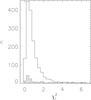 |
Fig. 3 The histogram of the reduced χ2 |

Using the procedure outlined in the previous Section, we were able to obtain a FTF for 1630 galaxies. The distribution of the  obtained for these fits is shown in Fig. 3: the median value is
  and 92% of the spectral fits satisfy
  .
.
For our sample, the DL07 dust model fits result in the following parameter ranges. γ ranges between 0.0 and 0.02 with a median value equal to 0.01; 75% of the sample have Umin in the range between 0.2 to 3.0, with a typical value equal to 1.5; qPAH shows a typical value 3.19, and 91% of the sample are best fit with templates based on Milky Way models (see Appendix A for more details).
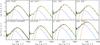 |
Fig. 4 Examples of DL07 spectral energy distribution (SED) fits to galaxies in our sample, as named in each panel. Photometric data points are shown with red circles and corresponding black error bars. Panels are organized (left to right) by the number of photometric data points (4 to 7 points). The top (bottom) row shows “normal” star forming (starburst; SB) galaxies; (see Sect. 4.3). The single best-fit DL07 template SED is shown in yellow. All SEDs which satisfy the reduced χ2 criterion (see Sect. 3) are shown in gray; the weighted geometric mean of these is used as our FTF (shown in black). The two temperature component model fits (Eq. (7)) are shown in red (cold dust component), blue (warm dust component), and green (sum of cold and warm dust components). |
 |
Fig. 5 Left panel: composite SEDs of galaxies with normal sSFR (875 normal star forming galaxies; red) and high sSFR (26 SB galaxies; blue), for wavelengths between 10 and 1000 μm. The orange spectrum is from a subsample (277 templates) of the normal galaxies closest to the MS (− 0.5 < sSFR [yr-1] < 0.5, see Sect. 4.3). Similarly, the purple spectrum is a subsample (11 templates) of the most extreme SB galaxies in our sample (sSFR [yr-1] > 0.8). Middle panel: comparison of composite SED of the subsample of galaxies closest to the MS (orange) with templates of Sa and Sc galaxies (black and green, respectively, obtained from the SWIRE template library, see text). Right panel: comparison of composite SED of the subsample of the most extreme SB galaxies (purple) with spectra of Arp 220 (a starburst-ULIRG; gray), IRAS 22491-1808 (a starburst-ULIRG; green), and IRAS 19254-7245 South (a Seyfert 2-starburst-ULIRG; black). In all panels, the composite spectra are plotted using solid lines, and their corresponding dispersions (± 0.7σ) are plotted using dotted lines of the same color. All SEDs are normalized to the 25 μm luminosity (νLν25 μm) in order to best contrast changes in the SED peak (~100 μm), sub-mm luminosities, and PAH emission at ~ 5 to 11 μm. Note that our fits use data between 12 μm and 850 μm. Further, our composite spectra do not include a stellar component, and thus do not match the comparison spectra below ~ 10 μm. |
Figure 4 shows eight example SED fits – both DL07 model fits and two temperature component fits – to galaxies in our sample. Clearly, when observed fluxes at ≤25 μm are absent, a large number of DL07 templates can be fitted: these templates show large differences at λ< 60 μm, but are similar at wavelengths in the Rayleigh-Jeans tail (λ> 300 μm). However, as shown by the robustness test (Sect. 4.2 and Appendix B) for a two-temperature component fit, the warm dust component (blue spectrum) is not affected by the absence of an observed flux at ≤25 μm if we follow our fitting criteria (see Sect. 3 and Appendix B). In a similar way, the cold dust component (red spectrum) does not vary significantly between different templates, as long as the galaxy has at least one measurement in the Rayleigh-Jeans tail. The figure also illustrates that the two temperature component model (green spectrum) reproduces well both the best fit SED (yellow spectrum) and the final template fit used by us (FTF; black spectrum).
To obtain the typical SEDs of galaxies with normal (MS) and high (SB) sSFR, we use the geometric mean (weighted by χ2) of all MS and SB galaxies. The left panel of Fig. 5 shows the composite SED of all 875 MS galaxies (red spectrum) and all 26 SB galaxies (blue spectrum), where the SB galaxies have sSFR> 0.8 [yr-1]. We also show the composite SEDs of two “cleaner” sub-samples: those closest to the MS (0.8 <sSFR [yr-1] < 1.2, orange spectrum) and those with the highest SFR in our sample (sSFR> 1.6 [yr-1], purple spectrum).
For each individual composite (MS and SB, Fig. 5 – middle panel) SED, the dispersions are small in the RJ tail: they are thus easily distinguishable from one another at wavelengths longer than λ> 200 μm, as long as a good short-wavelength (~25 μm) point is available for relative normalization. The largest differences between the two template spectra are seen near the FIR peak: high sSFR (SB) galaxies have a more dominant warm dust component: thus their emission peak is shifted to smaller wavelengths and the width of the peak is larger.
To compare our composite SEDs to those of galaxies with well characterized SEDs, we use the spectra available in the SWIRE template library (Polletta et al. 2007)8. The SWIRE templates, which are based on the GRASIL code (Silva et al. 1998), contain SEDs for ellipticals, spirals, and starburst galaxies.
The composite SED of our galaxies closest to the MS is compared to templates of Sa (black line) and Sc (green line) spiral galaxies (the Sb template is not shown as it is very similar to that of Sa galaxies) in the middle panel of Fig. 5. Clearly, there is a good agreement – within the 3σ dispersion – for λ> 10 μm; at shorter wavelengths the stellar component, present in the Sa and Sc templates but not in our MS composite, is the main reason for the observed differences. The composite SED of our highest sSFR subsample is compared to the spectrum of Arp 220 (gray), IRAS 22491–1808 (green) and IRAS 19254–7245 South (black) in the right panel of Fig. 5. The latter three spectra show a shift of the emission peak to shorter wavelengths compared to our SB composite SED, and IRAS 22491–1808 and IRAS 19254–7245 South show large absorption features at λ< 25μm which are not seen in our composite SED or indeed in any individual DL07 template.
4.2. Robustness of the SED fitting
To test the robustness of our SED fitting, we examine 24 galaxies of our sample with 7 photometric observations. Then, we explore how the Mdust , LIR , dust temperatures (cold and warm), quantity of SEDs, χ2 and reduced χ2 vary with the amount of points and the rejection of specific points (e.g., how it is affected by the rejection of the flux at 12 and 22 μm or at 350 μm). The result of this test reveals that our results are very robust, with the parameters showing factors of difference smaller than 0.1 (for Mdust , LIR , and dust temperatures). This means that the final results and relations obtained in our work, are robust and not affected by the amount of points or the distribution in wavelengths of them (following our SED fitting criteria, see Sect. 3). For more details, we refer to Appendix B.
4.3. Star formation mode
The SFR is often estimated from the IR (integrated between 8 to 1000 μm) and ultraviolet (λ = 2700 Å) luminosities (e.g., Murphy et al. 2011; Santini et al. 2014). Santini et al. (2014) suggest that both luminosities together provide the best estimate of SFR, but if only one is available, then LIR , rather than UV luminosity, is the more reliable. We estimate the SFR for our sample galaxies using LIR derived from our DL07 model fits and the relationship in Kennicutt (1998, assumes a Salpeter initial mass function) which assumes a ![Mathematical equation: \begin{equation} {\it SFR}~\left[\frac{\msun}{\rm yr}\right]=1.78\times10^{-10}~\lir~\left[L_{\odot}\right]. \label{eq:sfr} \end{equation}](/articles/aa/full_html/2017/06/aa29009-16/aa29009-16-eq179.png) (9)The top panels of Fig. 6 show the LIR distribution (black histogram) for our full sample. Infrared luminosities are 3.9 × 10⁶ to 7.0 × 10¹¹L⊙ with a typical error of 13% and median value of 2.2 × 10¹⁰L⊙. Comparing the LIR measured for the KINGFISH galaxies and our final sample with good SED fitting, we obtain a median ratio of 1.4. The bottom panel in Fig. 6 shows the distribution of the stellar mass (M∗), which ranges between 3.5 × 10⁸ and 7.9 × 10¹¹M⊙ with a median value of 3.6 × 10¹⁰M⊙ and typical error of 20%.
(9)The top panels of Fig. 6 show the LIR distribution (black histogram) for our full sample. Infrared luminosities are 3.9 × 10⁶ to 7.0 × 10¹¹L⊙ with a typical error of 13% and median value of 2.2 × 10¹⁰L⊙. Comparing the LIR measured for the KINGFISH galaxies and our final sample with good SED fitting, we obtain a median ratio of 1.4. The bottom panel in Fig. 6 shows the distribution of the stellar mass (M∗), which ranges between 3.5 × 10⁸ and 7.9 × 10¹¹M⊙ with a median value of 3.6 × 10¹⁰M⊙ and typical error of 20%.
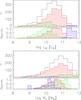 |
Fig. 6 Distribution of LIR (from the DL07-model-fits; top panels) and stellar mass (following Cluver et al. 2014; bottom panels) for our sample. Histograms for our full sample (black), all SBs (blue), all MS (red) and all passive galaxies (green) are shown. The bottom sub-panels show the equivalent normalized histograms. |
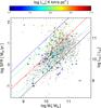 |
Fig. 7 The star formation rate – stellar mass plane. Interacting galaxies are shown with Xs, and non-interacting galaxies (or those which we were unable to classify due to lack of deep imaging) with circles. Symbol colors indicate the CO J:1-0 luminosity, with gray denoting galaxies without global CO J:1-0 measurements. The red solid line shows the MS locus from Elbaz et al. (2011), and the red dotted line shows the MS locus from Elbaz et al. (2007). The other lines delineate the limits used to classify our sample in starburstiness: SB galaxies lie above the blue solid line; Intermediate-SB (InSB) galaxies lie between the blue solid and green dashed lines; normal star forming galaxies (MS) lie between the green dashed and the cyan dashed lines; and PAS galaxies lie below the black solid line. The typical error is shown in the bottom right corner. |
Figure 7 shows all our sample galaxies in the SFR-M∗ plane. The sample covers roughly three orders of magnitude in both SFR and stellar mass, and are distributed on both sides of the locus of the Elbaz et al. (2011) MS line. Given the cutoffs in sSFR we use for SB, MS, and passive galaxies (see Sect. 1), the percentages of these sub-groups in our sample are 2.0%, 58.9%, and 15.%, respectively. In an equivalent manner, the Elbaz et al. (2007) MS (dotted red line in Fig. 7) is used and the same sSFR displacements from the MS are used to define MS, SB, and PAS galaxies. We see no great changes in the number of MS galaxies. However, the number of SBs increases (factor 1.8) and PAS galaxies decrease (factor 4.6).
4.4. Dust masses, temperatures, and emissivity index (β)
The presence of multiple dust temperatures in the DL07 models (see Sect. 3) precludes the direct application of Wien’s law to the model template (and thus our FTF) in order to obtain a dust temperature. For this reason we use two temperature component model fits to the FTF to parameterize the dust temperature (see Sect. 3). Figure 8 shows the distributions of the gray-body emissivity index (β), the temperatures of the cold (Tcold) and warm (Twarm) dust components in the two temperature component fits, (Eq. (7)), and the luminosity weighted dust temperature (Tweight, Eq. (6)). In agreement with previous results (e.g., Dunne & Eales 2001; Clements et al. 2010; Clemens et al. 2013) for nearby galaxies, our fitted values of β are distributed over 1.3–1.9, with a median of ~1.7 (Fig. 8). The β distributions for the sSFR-classified sub-samples are significantly different: PAS galaxies show the lowest values (median β ~ 1.4), MS galaxies typically show values in the range β = 1.3–1.9 with ⟨ β ⟩ ~ 1.7, and SB galaxies typically show values of β = 1.7 to 1.9 with ⟨ β ⟩ ~ 1.9. Similar differences are seen in the distributions of, and median, temperatures of the cold dust component: the median temperature of the cold dust component is 21.4 K for PAS galaxies, 23.6 K for MS galaxies, and 27.1 K for SB galaxies.
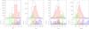 |
Fig. 8 From left to right: distributions of the emissivity index (β), the temperatures of the cold (Tcold) and warm (Twarm) dust components, and the luminosity-weighted dust temperature (Tweight). In all panels, the distribution of the full sample is shown in black, SB galaxies in blue, MS galaxies in red, and PAS galaxies in green. The lower panels show the equivalent normalized histograms. |
For the full sample, the warm dust component (from the two component fit; Fig. 8) shows a median value of Twarm = 57 K. Unexpectedly, the PAS galaxies show the hottest warm components, though the relative luminosity of this warm component is neglible with regards to the luminosity of the cold component. MS galaxies have warm component temperatures distributed relatively tightly around Twarm = 57 K while SB galaxies show a more uniform spread in the distribution of Twarm . In relative luminosity, however, the SBs are more dominated by the warm dust component: SB and MS galaxies show a median warm component luminosity to total luminosity (cold plus warm component) ratio of 0.01 and 0.14, respectively. If, instead, the FTF is characterized by the weighted dust temperature, the full sample shows a median weighted temperature of 24.1 K. PAS, MS and SB galaxies are clearly separated in Tweight, with median values of 21.0, 25.2 and 31.1 K, respectively.
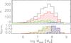 |
Fig. 9 Distribution of the DL07-model-derived dust mass. The full sample is shown in black, and the sub-samples of SB, MS, and PAS galaxies are shown with the same colors as in Fig. 8. The bottom panel shows the equivalent normalized histograms. |
Figure 9 shows the distribution of the dust masses, as derived from the DL07 model fits (see Sect. 3), for the entire sample (black), and for the different sSFR sub-samples (SB in blue, MS in red and PAS in green). In the full sample, dust masses range between 6.2 × 10⁵M⊙ and 8.6 × 10⁸M⊙, with a median value of 7.5 × 10⁷M⊙ and an estimated typical error of 20%. This median value is similar (considering our errors) to that obtained by Clemens et al. (2013; 7.8 × 10⁷M⊙), who used MAGPHYS modeling. Note that they corrected their model results to an emissivity value of κ850 = 0.0383 m2 kg-1, the same value assumed in our dust mass estimations from two dust components and in agreement with the results obtained with the DL07 templates (see below). Passive galaxies tend to have lower dust masses than MS and SB galaxies. The median dust mass for PAS, MS, and SB galaxies are 6.2 × 10⁷, 7.6 × 10⁷, and 1.7 × 10⁸M⊙, respectively. For the two temperature component models, the cold dust component dominates the total dust mass: the median contribution of warm dust to the total (warm plus cold) dust mass (Mw/Mtot) is 0.2%, with 97% of the sample at Mw/Mtot< 1%. The highest values of Mw/Mtot (up to 4%) are seen in SB galaxies.
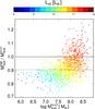 |
Fig. 10 Ratio of dust masses (two component fit to DL07 model fit) as a function of DL07 model fit dust masses. SBs, MS, and PAS galaxies are plotted as diamonds, squares, and crosses, respectively. Upward and downward triangles show intermediate SB and intermediate PAS sources. The line of equality (solid black line) and median ratio (dashed black line) are also shown. Symbols are colored by IR luminosity following the color-bar. |
A comparison of the dust masses derived using DL07 models to the dust masses derived from our two component  ; Eq. (8) fits is shown in Fig. 10. Clearly there is a systematic difference in the two values. Recall that the two component model was obtained via fits to the DL07 FTF fit rather than a fit to the individual photometric data points. The dust mass ratios
  show a median of 0.91, and the best fit relating the two dust masses (see Fig. 10) is:
 ![Mathematical equation: \begin{equation} \frac{M^{\rm 2gb}_{\rm dust}}{[\msun]}=10^{-0.34\pm0.06} \left(\frac{M^{\rm DL07}_{\rm dust}}{[\msun]}\right)^{1.04\pm0.01} . \end{equation}](/articles/aa/full_html/2017/06/aa29009-16/aa29009-16-eq205.png) (10)The symbol colors (by IR luminosity) clearly reveal that the inconsistency in the DL07 and two-component derived dust masses is correlated to the IR luminosity: sources with lower LIR show relatively higher DL07 model dust masses, while sources with higher LIR have relatively higher two gray-body-fit dust masses. Alternatively, the difference in the two masses is related to the dust temperature of the cold component, showing an increment from the bottom left corner to the right top corner for the points in the figure. The difference in masses is likely a result of the DL07 models using a more complex calculation of dust mass for a given dust luminosity, that is, different grain types and sizes related to the parameter qPAH (see details in Draine et al. 2007), while the dust mass of the two temperature component fit is derived via a single emissivity index. In any case, the difference in dust masses is less than 0.2 dex (factor of 1.58), so these differences are relatively unimportant in the correlations presented in the following sections (which use the DL07-derived dust masses).
(10)The symbol colors (by IR luminosity) clearly reveal that the inconsistency in the DL07 and two-component derived dust masses is correlated to the IR luminosity: sources with lower LIR show relatively higher DL07 model dust masses, while sources with higher LIR have relatively higher two gray-body-fit dust masses. Alternatively, the difference in the two masses is related to the dust temperature of the cold component, showing an increment from the bottom left corner to the right top corner for the points in the figure. The difference in masses is likely a result of the DL07 models using a more complex calculation of dust mass for a given dust luminosity, that is, different grain types and sizes related to the parameter qPAH (see details in Draine et al. 2007), while the dust mass of the two temperature component fit is derived via a single emissivity index. In any case, the difference in dust masses is less than 0.2 dex (factor of 1.58), so these differences are relatively unimportant in the correlations presented in the following sections (which use the DL07-derived dust masses).
4.5. LIR, Mdust and tdust plane
The relationship between dust mass, dust temperature, and dust luminosity (LIR) is in general well understood (e.g., Draine & Li 2007; Scoville 2013): when dust grains absorb UV photons from young OB stars, they are heated and re-emit their energy at IR wavelengths. Clemens et al. (2013) have shown a strong correlation between the SFR/Mdust ratio and the dust temperature of the cold dust component, especially for sources with Tdust,cold> 18 K. Our sample shows a similar correlation, and our larger sample size allows us to clearly demonstrate that all galaxies lie in a single plane, which we refer to as the dust plane, in the LIR (thus SFR), Mdust and Tdust phase space (similar to the relation shown by Genzel et al. 2015).
Figure 11 shows a projection of this dust plane in our sample: in this case we plot LIR against Mdust and color the symbols by the (cold component) dust temperature. The dashed black lines delineate the LIR –Mdust relationships for different cold component dust temperature bins, and the purple line shows the relation between LIR and Mdust obtained by da Cunha et al. (2010). Here the dust temperature used is that of the cold component of the two component fit; this is the dominant component, in mass and luminosity, for all galaxies in the sample. The best fit to this dust plane is: ![Mathematical equation: \begin{equation} \log \left(\frac{L_{\rm IR}}{[\lsun]}\right) - 1.07 ~\log \left(\frac{M_{\rm dust}}{[\msun]}\right)- 0.19 ~\left(\frac{T_{\rm cold}}{\rm [K]}\right) + 2.53 = 0 \label{eq:plane} . \end{equation}](/articles/aa/full_html/2017/06/aa29009-16/aa29009-16-eq210.png) (11)Clearly, the placement of a galaxy in the dust plane is most sensitive to the temperature of the cold component, rather than the values of Mdust and LIR . For example, if the dust temperature is constant and we change Mdust by a factor of 10, the LIR is required to change by a factor of 12. However, increasing Tcold by 10 K, with constant Mdust , requires LIR to increase by a factor 80. An increase in LIR is more easily achieved by increasing the dust temperature rather than the dust mass. The data of Clemens et al. (2013) are consistent with a plane similar to that defined by Eq. (11). However, their data suggest higher values of both LIR and Mdust for a given value of Tcold .
(11)Clearly, the placement of a galaxy in the dust plane is most sensitive to the temperature of the cold component, rather than the values of Mdust and LIR . For example, if the dust temperature is constant and we change Mdust by a factor of 10, the LIR is required to change by a factor of 12. However, increasing Tcold by 10 K, with constant Mdust , requires LIR to increase by a factor 80. An increase in LIR is more easily achieved by increasing the dust temperature rather than the dust mass. The data of Clemens et al. (2013) are consistent with a plane similar to that defined by Eq. (11). However, their data suggest higher values of both LIR and Mdust for a given value of Tcold .
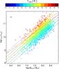 |
Fig. 11 Relationship between IR luminosity (thus SFR) and dust mass for our sample, with the symbols colored by the temperature of the cold dust component. The figure is a projection of the dust plane we find between LIR , Mdust , and Tcold . Symbols – which denote the sSFR classification of the galaxies – are the same as in Fig. 10. The black dashed lines are the fits to the LIR –Mdust plane for cold component dust temperature bins centered at (bottom to top) 20, 22, 24, 26 and 28 K. The purple line shows the relationship between LIR and Mdust obtained by da Cunha et al. (2010) where dust temperature is not taken into account. The typical error is shown in the top right of the plot. |
If the luminosity weighted dust temperature (Tweight) is used instead of Tcold , the sample galaxies still fall on a single dust plane, though there is a larger scatter. In this case, the dust plane is parametrized by: ![Mathematical equation: \begin{equation} \log \left(\frac{L_{\rm IR}}{[\lsun]}\right) - 1.02 ~\log \left(\frac{M_{\rm dust}}{[\msun]}\right)- 0.10 ~\left(\frac{T_{\rm weight}}{\rm [K]}\right) + 0.30 = 0 \label{eq:plan1e2} . \end{equation}](/articles/aa/full_html/2017/06/aa29009-16/aa29009-16-eq211.png) (12)If the temperature of the warm component (from the two components fit) of the dust is used instead of the temperature of the cold component, the sample galaxies no longer fall on a single dust plane.
(12)If the temperature of the warm component (from the two components fit) of the dust is used instead of the temperature of the cold component, the sample galaxies no longer fall on a single dust plane.
The correspondence between interacting galaxies and SB galaxies is one-to-one only for extreme starbursts: of all interacting galaxies in the sample, only those with high cold-dust component temperature (Tcold> 27 K) and high SFR (log (LIR/L⊙) > 11, that is, LIRGs) are classified as SBs.
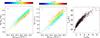 |
Fig. 12 Left and middle panels: dependence of the dust mass and IR luminosity on the 350 μm monochromatic luminosity. Symbol colors show the temperature of the cold dust component, and the blue line shows the best fit. The typical error is shown by the black cross. Equivalent figures for monochromatic luminosities at 550 μm and 850 μm can be found in Appendices E and F. Right panel: correlation between the temperature of the cold dust component and the 100 μm to 350 μm flux ratio, with the best fit shown by the dashed blue line. Large, red crosses show the mean value of Tcold in 0.5 mag color bins, and the red dashed curve corresponds to the best fit line to the red crosses. The typical error in the x-axis is shown by the black horizontal line. Similar plots relating Tcold to IR and sub-mm colors can be found in Appendix D. In all panels the symbols are the same as in Fig. 10. |
While the dust plane provides a powerful tool to relate the dust mass, total IR luminosity and dust temperature of the cold component, or derive any one parameter from the other two, the comprehensive dataset available for our large local sample is difficult to obtain for other samples, especially those at high redshift. We thus provide several scaling relationships which can be used to estimate the location of a galaxy in the dust plane in the presence of limited data or, alternatively, to derive one or all parameters of the dust plane phase space.
Since the dust plane is most sensitive to changes in Tcold , we present several relations to estimate its value using sub-mm to IR colors. Previous works, for example, Soifer et al. (1987), Chanial et al. (2007), Hwang et al. (2010), have typically derived dust temperatures from IRAS colors: IRAS 60/IRAS 100. Here we present that based on the 100 μm and 350 μm color; we refer to Appendix D for the equivalent results from other IR to sub-mm colors. The relationship between the cold component dust temperature and the 100 μm to 350 μm flux ratio is shown in the right panel of Fig. 12. The best fit to this relationship is: ![Mathematical equation: \begin{equation} \frac{T_{\rm cold}}{\rm [K]}=10^{(1.280\pm0.001)}\left(\frac{\emph{f}_{100}}{\emph{f}_{350}}\right)^{(0.160\pm0.001)} \label{eq:tcold f350-f100} . \end{equation}](/articles/aa/full_html/2017/06/aa29009-16/aa29009-16-eq215.png) (13)To obtain a cleaner relation, large crosses in Fig. 12 show the mean value of Tcold in bins of 0.5 mag in the color f100/f350. Interestingly, the coefficients of the best fit (red dashed line) show that the values are consistent within the errors with the coefficients obtained for the complete sample.
(13)To obtain a cleaner relation, large crosses in Fig. 12 show the mean value of Tcold in bins of 0.5 mag in the color f100/f350. Interestingly, the coefficients of the best fit (red dashed line) show that the values are consistent within the errors with the coefficients obtained for the complete sample.
Both the dust mass and the total IR luminosity can be estimated from a single monochromatic luminosity in the RJ tail of the dust emission. The dependence of Mdust and LIR on the 350 μm luminosity is shown in the left and middle panels of Fig. 12, respectively. At first glance, these relationships appear to have a large scatter. However, it is clear that this scatter can be fully explained (and removed) by the use of the temperature of the cold dust component. Thus the estimation of Mdust and/or LIR can be made very accurately in the presence of an estimate of the cold dust temperature (see previous paragraph) or at least roughly in the absence of a cold dust temperature. We will address both scenarios below for the case of using the 350 μm luminosity for the RJ tail luminosity (see Appendices E and F for the results of using other sub-mm frequencies).
Using the monochromatic luminosity at 350 μm in the presence of a value for Tcold , we obtain two planes to determinate LIR or Mdust : ![Mathematical equation: \begin{eqnarray} \log \left(\frac{L_{\rm IR}}{[\lsun]}\right) & -& 1.017~ \log \left(\frac{L_{350}}{\rm [W~Hz^{-1}]}\right) \nonumber \\ & -& 0.118~ \left(\frac{T_{\rm cold,~dust}}{\rm [K]}\right) + 16.45 = 0 \\ \log \left(\frac{M_{\rm dust}}{[\msun]}\right) & -& 0.940~ \log \left(\frac{L_{350}}{\rm [W~Hz^{-1}]}\right) \nonumber \\ & +& 0.0791~ \left(\frac{T_{\rm cold,~dust}}{\rm [K]}\right) + 12.60 = 0. \nonumber \label{eq:lir-mdust with l350 and td} \end{eqnarray}](/articles/aa/full_html/2017/06/aa29009-16/aa29009-16-eq217.png) (14)In the absence of a Tcold estimation, one has to accept the full scatter seen in the left and middle panels of Fig. 12, that is, a dispersion of 0.5 dex and 1 dex in the estimation of Mdust and LIR from a single 350 μm luminosity. The best fit to the data points (blue lines in Fig. 12, right and middle panels) is:
(14)In the absence of a Tcold estimation, one has to accept the full scatter seen in the left and middle panels of Fig. 12, that is, a dispersion of 0.5 dex and 1 dex in the estimation of Mdust and LIR from a single 350 μm luminosity. The best fit to the data points (blue lines in Fig. 12, right and middle panels) is: ![Mathematical equation: \begin{eqnarray} \frac{L_{\rm IR}}{[\lsun]} & = & 10^{-14.388\pm0.002} \left(\frac{L_{350}}{\rm [W~Hz^{-1}]}\right)^{1.046\pm0.005}\\ \frac{M_{\rm dust}}{[\msun]} &=& 10^{-13.963\pm0.002} \left(\frac{L_{350}}{\rm [W~Hz^{-1}]}\right)^{0.920\pm0.005}\nonumber\cdot \label{eq:lir-mdust with l350} \end{eqnarray}](/articles/aa/full_html/2017/06/aa29009-16/aa29009-16-eq218.png) (15)Estimations of the dust mass and IR luminosity from other monochromatic IR or sub-mm fluxes, and estimates of the temperature of the cold dust component from other IR and sub-mm colors can be found in Appendices D, E, and F.
(15)Estimations of the dust mass and IR luminosity from other monochromatic IR or sub-mm fluxes, and estimates of the temperature of the cold dust component from other IR and sub-mm colors can be found in Appendices D, E, and F.
4.6. Dust to stellar mass ratio
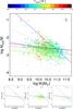 |
Fig. 13 Top panel: dust to stellar mass ratio ( |

The typical Mdust/M∗ ratios are 0.21% and 0.25% for our entire sample and for all star forming (non-passive) galaxies, respectively. These ratios are smaller than those obtained by Clemens et al. (2013; median Mdust/M∗ = 0.46% in a well defined sample of 234 nearby galaxies detected by Planck) and Clark et al. (2015; median Mdust/M∗ = 0.44% in the HAPLESS sample, a blind sample of 42 nearby galaxies detected by Herschel). Another three works, using the MAGPHYS code, show similar values for the dust to stellar mass ratio. da Cunha et al. (2010) shows a value between 0.23% and 0.14% depending on the stellar mass bin used in a sample of 1658 galaxies at z< 0.1; Smith et al. (2012) obtain a dust to stellar mass of 0.22% from a sample of 184 galaxies at z< 0.1; while Pappalardo et al. (2016) show a value of 0.18% in their main sample.
An anticorrelation between the Mdust /M∗ and M∗ has been shown by Cortese et al. (2012, in Virgo cluster galaxies), Clemens et al. (2013) and Clark et al. (2015).
We see the same anticorrelation in our sample (Fig. 13), with the points showing a large dispersion. The fits to our full sample (FS; purple line) and to all our star forming (SF) galaxies (non-passive galaxies; black line), are: ![Mathematical equation: \begin{eqnarray} \frac{M_{\rm dust}}{M_*}& =& 10^{-0.4\pm0.2} \left(\frac{M_*}{[\msun]}\right)^{-0.28\pm0.02}~~ \rm FS\\ \frac{M_{\rm dust}}{M_*} &=& 10^{-1.3\pm0.2} \left(\frac{M_*}{[\msun]}\right)^{-0.12\pm0.02}~~ \rm SF.\nonumber \end{eqnarray}](/articles/aa/full_html/2017/06/aa29009-16/aa29009-16-eq223.png) (16)When we separate the galaxies by star-forming mode (bottom panels of Fig. 13), we find two interesting results: (a) SB galaxies show a much steeper anticorrelation than the other sub-samples, and (b) the source of the scatter in the anticorrelation can be traced by the temperature of the cold dust component, Tcold (or the weighted dust temperature Tweight). The anticorrelations obtained individually for each subsample are:
(16)When we separate the galaxies by star-forming mode (bottom panels of Fig. 13), we find two interesting results: (a) SB galaxies show a much steeper anticorrelation than the other sub-samples, and (b) the source of the scatter in the anticorrelation can be traced by the temperature of the cold dust component, Tcold (or the weighted dust temperature Tweight). The anticorrelations obtained individually for each subsample are: ![Mathematical equation: \begin{eqnarray} \frac{M_{\rm dust}}{M_*}&=& 10^{7.4\pm0.8} \left(\frac{M_*}{[\msun]}\right)^{-0.92\pm0.08} ~~\rm SB\nonumber\\ \frac{M_{\rm dust}}{M_*}&= & 10^{-2.1\pm0.2}\left(\frac{M_*}{[\msun]}\right)^{-0.09\pm0.01} ~~\rm MS\\ \frac{M_{\rm dust}}{M_*}&=& 10^{-1.2\pm0.4}\left(\frac{M_*}{[\msun]}\right)^{-0.17\pm0.04} ~~\rm PAS.\nonumber \end{eqnarray}](/articles/aa/full_html/2017/06/aa29009-16/aa29009-16-eq224.png) (17)Essentially, the dust to stellar mass ratio in SB galaxies (typically 1.3%) is higher than that in MS galaxies (typically 0.24%), though the difference is smaller for galaxies at the highest stellar masses. Passive galaxies show a very low dust to stellar mass ratio, with a typical value of Mdust/M∗ = 0.1%. Additionally, for all sSFR groups, at a given stellar mass, the galaxies with the highest Tcold (Tweight) have the smaller dust to stellar mass ratios.
(17)Essentially, the dust to stellar mass ratio in SB galaxies (typically 1.3%) is higher than that in MS galaxies (typically 0.24%), though the difference is smaller for galaxies at the highest stellar masses. Passive galaxies show a very low dust to stellar mass ratio, with a typical value of Mdust/M∗ = 0.1%. Additionally, for all sSFR groups, at a given stellar mass, the galaxies with the highest Tcold (Tweight) have the smaller dust to stellar mass ratios.
4.7. Dust to gas mass ratio
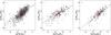 |
Fig. 14 Relationships between dust mass and atomic gas mass (left), molecular gas mass (middle) and total ISM mass (right). Black symbols are used for galaxies with HI and CO observations and dust mass from DL07 models; red symbols are used for galaxies with HI and CO observations, but with dust masses estimated from the luminosity at 350, 550 or 850 μm (see Eq. (16) and Appendix F); Gray symbols denote galaxies with either HI or CO observations and dust mass from DL07 models. The solid black lines in each panel show the best fit to all sources with measurements of both MHI and Mmol, and the gray dashed lines in the two left panels show the fit to all points in the respective panel. The typical error is shown by the black cross in each panel. |
To more easily study the relation between dust and gas masses, we separate the total gas mass (hereafter referred to as interstellar medium mass or MISM ) into two components: the molecular gas mass (Mmol), and the atomic (hydrogen) gas mass (MHI): MISM = Mmol + MHI. Figure 14 shows the relation between the dust mass and the atomic (left panel), molecular (middle panel) and total (right panel) gas masses.
The median gas fraction (MISM/ (M∗ + MISM)) for the full sample is 33 ± 11%. The medians for MS, PAS, and SB galaxies are 32 ± 8%, 5.0 ± 0.8% and 68 ± 25%, respectively. For all sources with HI and CO measurements, the molecular to atomic gas mass ratios (Mmol/MHI) show a median value of 0.8 ± 0.2. Even for MS and PAS galaxies, the same value is observed, however SB galaxies show a huge value (4 ± 1; see Table 3).
Sources with measurements in both MHI and Mmol.
Sources with measurements in MHI or Mmol.
The median values of Mdust/MHI are 1.6% and 1.3% for the galaxies with both MHI and Mmol and for those with only MHI measurements, respectively (see Tables 3 and 4). These values are smaller than those obtained by Clements et al. (2010,2.2%) and Clark et al. (2015,3.9%). PAS galaxies show the highest dust to atomic mass ratios, followed by SB and finally MS galaxies. The median dust to molecular gas mass ratio is 2.1% for all galaxies with both MHI and Mmol, and 2.0% for all galaxies with only Mmol. Passive galaxies show the largest dust to molecular gas mass ratios followed by MS galaxies, with SB galaxies showing the lowest values. The median dust to ISM mass ratios are similar for the full sample, MS, and SB galaxies (0.8%, 0.7%, and 0.6%, respectively), while PAS galaxies show larger values (1.4%).
Figure 14 shows a clear correlation between dust mass and molecular and atomic gas mass, individually. But the correlation between dust and MISM shows the smallest dispersion, with the best fit: ![Mathematical equation: \begin{equation} \frac{M_{\rm ISM}}{[ M_{\odot}]}=6.03 \left(\frac{M_{\rm dust}} {[ M_{\odot}]}\right)^{0.7} \label{eq:mdust-mism fit} \cdot \end{equation}](/articles/aa/full_html/2017/06/aa29009-16/aa29009-16-eq261.png) (18)This correlation between ISM and dust mass has been noted previously by Leroy et al. (2011, in five Local Group galaxies) and Corbelli et al. (2012, in 35 metal-rich Virgo spirals).
(18)This correlation between ISM and dust mass has been noted previously by Leroy et al. (2011, in five Local Group galaxies) and Corbelli et al. (2012, in 35 metal-rich Virgo spirals).
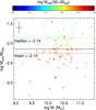 |
Fig. 15 Dust to ISM mass ratio as a function of stellar mass. Symbols are the same as in Fig. 10 and colors represent the gas fraction. The black solid and dashed lines show the median and mean dust to gas ratios, respectively, for the entire sample. Colored solid lines show median values for SB (blue), MS (red), and PAS (green) galaxies. The black cross shows the typical error. |
The dust to gas ratio (δDGR = Mdust/MISM) does not systematically vary with the stellar mass for our sample galaxies (Fig. 15), despite the expected metallicity range (between 8.4 and 9.1) for this stellar mass range (109 < M∗ [M⊙] < 1011) (Tremonti et al. 2004). Our full sample shows a large scatter in δDGR (±0.5 dex), but the scatter significantly decreases when considering SB, MS, and PAS galaxies separately. MS and PAS galaxies show a dispersion in δDGR of ±0.3 dex, and SBs show a dispersion of only ±0.2 dex. The median values of δDGR for MS and SB galaxies (red and blue lines in Fig. 15, respectively) are very similar to the median value of the full sample; however, PAS galaxies show a higher median δDGR (green line in Fig. 15). Additionally, the symbol colors show that the galaxies with higher gas fractions have lower values of δDGR, especially MS and PAS galaxies.
5. Discussion
We have modeled the dust emission using detailed DL07 dust models in an unprecedentedly large sample of 1630 nearby (z< 0.1, ⟨ z ⟩ = 0.015) galaxies with uniform photometric data from WISE (3.4 to 22 μm), IRAS (12 to 100 μm), Planck (350 to 850 μm) and/or SCUBA (850 μm). This sample covers a significant parameter space in stellar mass and SFR, and thus sSFR, going from starburst (SB; LIRGs; LIR> 1011L⊙) to passive (PAS; LIR ~ 108.3L⊙) galaxies.
In comparison, previous studies that present detailed dust models to galaxies with sub-mm data include the KINGFISH/SINGS sample (Dale et al. 2012) of 65 nearby, normal (LIR< 1011L⊙) spiral galaxies with photometry from IRAS, Spitzer, Herschel, and SCUBA, and the ERCSC sample Negrello et al. (2013), Clemens et al. (2013) of 234 local (z< 0.1) galaxies with photometry from IRAS, WISE, Spitzer, Herschel and Planck. The ERCSC sample was created by matching four Herschel samples, HRS, HeViCS, KINGFISH and H-ATLAS, to the Planck Early Release Compact Source Catalogue.
Note that the other large nearby sample of galaxies with dust modeling results, the sample of 1658 galaxies in da Cunha et al. (2010), used MAGPHYS modeling applied to UV, optical, and limited IR data (2MRS, IRAS); the lack of sub-mm data is expected to lead to less reliable dust mass estimates (e.g., Draine et al. 2007).
The advantages of our sample over the ERCSC sample include: a) a sample size approximately seven times larger with equivalent and consistent data observations; b) the use of the Second Planck catalog of Compact Sources, which contains only reliable detections (in this release the Planck collaboration separated the less reliable detections into a separate “excluded” catalog which we do not use); c) the fact that the catalogs of the Planck second release are deeper than those of the Early Release; d) the use of flux corrections to the Planck catalog fluxes (Nagar et al., in prep.) to ensure consistency with the SCUBA flux scale.
We remind the reader that all galaxies fitted with dust models had between four and seven photometric points distributed between 12 μm and 850 μm. In all cases these points populated both sides of the SED peak with ≥2 photometric points shortward of λ ≤ 100 μm and ≥ one photometric point at λ ≥ 350 μm. A further indication that the available number of photometric points sufficiently constrained the fitted SED is that all templates matched to the photometry with  have similar spectral shapes and parameters (such as Mdust or LIR ), despite the extremely large number of templates (24 200) in our work.
The differences in the dust masses obtained by us and those obtained by Draine et al. (2007, who used similar modeling but more extensive photometric data at λ ≤ 100 μm in 17 KINGFISH/SINGS galaxies, ranges between −0.3 dex and 0.4 dex, with a median of −0.07 dex. The equivalent differences in the IR luminosities obtained by us and those obtained by Draine et al. (2007) range between −0.017 dex and 0.5 dex with a median of 0.14 dex. The largest discrepancies are seen in galaxies (e.g., NGC 6946) for which Draine et al. (2007) did not use sub-mm data. Dale et al. (2012) explore the dust modeling in a larger KINGFISH/SINGS sample, which contains 64 galaxies with sub-mm fluxes. However, the dust masses and IR luminosities obtained from the model fits were not explicitly listed, thus we can not compare our results. Additionally, the values of LIR and LFIR calculated from the dust model fits are in overall agreement with those estimated from IRAS fluxes using the Sanders et al. (1991) equations. In fact, we use our SED-derived LIR and LFIR values to recalibrate the equations to estimate these values from only IRAS photometry (Appendix E).
The advantage of our sample compared to previous works listed in Table 1 is that, for the first time, we have a large amount of nearby galaxies (more than ten times larger than previous studies) with one or more sub-mm measurements. Additionally, as a consequence of the all-sky observation by Planck, our sample reduces its selection effects only to the cutoffs of Planck (its reliable zones), without selection effects for a specific type of galaxy (for example, the KINGFISH/SINGS sample, which contains only star forming galaxies).
5.1. Interpreting the dust temperature
We can interpret the dust temperature of the cold component (Tcold) as the equilibrium temperature of the diffuse ISM. This interpretation is supported by the strong correlation between Tcold and the starlight intensity parameter of the diffuse ISM (Umin) in DL07. This correlation has been demonstrated by Aniano et al. (2012, in a sample of two resolved galaxies) and used by Ciesla et al. (2014, in the HRS sample) to compare their SED fitting results with the results of other works. The problem with this interpretation is that the temperature of the diffuse ISM (thus Tcold ) is not expected to correlate with the SFR (produced in PDRs rather than the diffuse ISM). However, the dust plane shown here implies a close connection between LIR , Mdust , and Tcold (see Sect. 4.5). Furthermore, the SFR – M∗ relation also shows a dependence on Tcold ; Tcold increases as one moves from sources with higher M∗ and lower SFR to sources with lower M∗ and higher SFR. To solve this contradiction, Clemens et al. (2013) propose that the lower dust masses in star-forming regions allow the escape of UV photons thus increasing the starlight intensity impinging on the diffuse ISM, which in turn would increase its temperature.
In agreement with the Clemens et al. (2013) results, we find that LIR , Mdust , and other parameters do not correlate with the warm dust component temperature (Twarm). The parameters Umin and γ (the percentage of dust mass PDRs) show only a weak correlation with Twarm . Nevertheless, the importance of using a warm component is that when it is used, the cold component temperature (Tcold; rather than the temperature obtained from a single component fit) shows much cleaner correlations with LIR , Mdust , and the dust plane, and also better explains the systematics in, for example, the Mdust /M∗ versus M∗ anticorrelation. Further, Tcold , rather than, for example, Tweight, is more cleanly correlated with the IR to sub-mm colors.
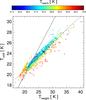 |
Fig. 16 A comparison of the temperature of the cold dust component (Tcold; from the two component fit) and the luminosity weighted temperature (Tweight) for our sample. The different symbols show SBs (diamonds), MS (squares), PAS (crosses), intermediate SB (upward triangles) and intermediate PAS (downward triangles) galaxies. Symbols are color-coded by the temperature of the warm dust component following the color bar. The dashed and solid lines show the best fit and the line of equality, respectively. |
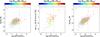 |
Fig. 17 Atomic hydrogen mass (left), |
It is useful to compare the luminosity weighted dust temperature (Tweight) with the temperatures obtained from the two component fits, since Tweight is independent of our assumptions made in the two-component fits. Figure 16 shows the relationship between Tweight and the Tcold ; the scatter in the data points is primarily correlated with Twarm . The tightest correlation is found for MS and PAS galaxies with Twarm≤ 58 K. SBs and Intermediate SB galaxies (typically at Twarm≥ 58 K) show a larger scatter. A cleaner correlation is observed if we compare Tweight with a temperature obtained from a weighted addition of Tcold and Twarm , where the weights are the respective flux fractions (e.g., Sc/ (Sw + Sc)). That is, the increase in the scatter seen in Fig. 16 for Twarm≥ 58 K is a consequence of the increment in the fractional flux of the warm component. The use of Tweight instead of Tcold in all the relevant relations presented in Sect. 4 produces similar results but with a larger scatter. Furthermore, IR and sub-mm colors (see Appendix D) can be used to estimate Tcold with a smaller scatter than Tweight.
We obtain a better estimation of the dust temperature of the cold component using a color. This color is based on a IR flux (λ< 100 μm) and a sub-mm (λ> 350 μm) flux. These estimates show a stronger relation than compared to using only two IR fluxes or only two sub-mm fluxes (e.g., the color 60 to 100 μm). The lowest end of our wavelength range (12 and 22 μm) shows the least reliable estimates of Tcold using an IR and sub-mm color. This is a consequence of the warm component influence within these fluxes. However, the Tweight shows a tight correlation with the color obtained using the flux at 22 μm and one sub-mm flux, but not with the color at 12 μm. This is a consequence of its proximity to the PAHs emission.
5.2. Dust mass as a tracer of total gas mass
Figure 17 shows the relationships between the atomic gas mass to stellar mass ratio, the to stellar mass ratio and the dust to stellar mass ratio, with the distance of the galaxy from the MS (log (sSFR/sSFRMS)). These plots reveal that log (sSFR/ sSFRMS) is weakly correlated with MHI and , but tightly correlated with the dust to stellar mass ratio.
The evolution of the dust to stellar mass ratio as tracer of star-formation mode (sSFR classification) was previously studied in galaxies within the redshift range 0 <z< 4 by Tan et al. (2014), who use different dust to stellar mass ratios for normal star forming galaxies and extreme SB galaxies (ULIRGs) over the redshift range 0 to 2. The largest difference was found at z ~ 0 where for normal galaxies they used the averaged value of the normal galaxies in the da Cunha et al. (2010) sample. In comparison, the normal galaxies in our sample show a large scatter (~1.3 dex) in their dust to stellar mass ratios (see right panel of Fig. 17), so that they overlap with the median dust to stellar mass ratio of extreme starbursts. This scatter is related to the gas fraction of these galaxies, where gas-rich galaxies show higher dust to stellar mass ratios. Our sample does show that SB and InSB galaxies have higher dust to stellar mass ratios than MS and PAS galaxies; in fact their dust to stellar mass ratios are higher than the data point of extreme SBs at z ~ 0 in Tan et al. (2014) even though our SBs and InSB samples are made up of LIRGs instead of ULIRGs. Thus overall, we observe median dust to stellar mass ratios higher than those used by Tan et al. (2014), and an overlap in the dust to stellar mass distributions of normal and SB galaxies.
Garn & Best (2010) have showed that galaxies with higher dust masses have higher stellar masses. However, in our work we reveal a more complex picture, in which the dust-to-stellar-mass ratio anticorrelates with the stellar mass, and the strength of the anticorrelation changes in sub-samples of galaxies separated by their star-forming mode (i.e., by sSFR; see Sect. 4.6). Thus, low-stellar-mass SB galaxies are dustier than massive PAS galaxies. This result is in agreement with the discussion in Clemens et al. (2013), where they conclude that despite (δDGR) and M∗ being directly proportional to metallicity (Z), galaxies with smaller M∗ show higher MISM/M∗ and this effect prevails over the tendency of galaxies with smaller M∗ to have smaller Z.
Passive galaxies of course show the lowest sSFR, dust to ISM mass ratios, and ISM to stellar mass ratios (Fig. 17). But Fig. 15 shows that even though PAS galaxies have smaller gas fractions, they have larger δDGR in comparison with MS and SB galaxies. That is, at low SFRs, decreasing SFR results in the ISM mass decreasing faster than the dust mass.
5.3. Estimating ISM mass from a single sub-mm measurement
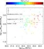 |
Fig. 18 Ratio of the monochromatic luminosity at 850 μm to the ISM mass as a function of monochromatic luminosity at 850 μm. Circles show galaxies of our sample and large triangles show galaxies from Scoville et al. (2014). Symbols are colored by the LIR following the color bar. The median value for our sample is shown by the dashed line, while dotted lines show the median values obtained by Scoville et al. (2014) and by Hughes et al. (2017). The black cross shows the typical error. |
The technique of using a single rest-frame monochromatic luminosity at 850 μm to obtain a reasonably accurate ISM mass, developed by Scoville (2013), Scoville et al. (2014, 2016), is based on two primary assumptions: (1) a constant δDGR for galaxies with M∗ between 109 and 1011M⊙, and (2) the assumption of a uniform dust temperature for all galaxies, justified because a change by factor ~ 2 in the dust temperature will introduce an error of only factor ~ 2 (0.3 dex) in the ISM mass. With these assumptions, α850 (=L850/MISM) can be used to convert a sub-mm luminosity to an ISM mass. In our sample, the median value of α850 is 12.56, with a rms of ~ 0.3 dex (Fig. 18). This value is 0.44 dex (factor 2.8) lower than that obtained by Scoville et al. (2014) and 0.15 dex (factor 1.4) lower than that obtained by Hughes et al. (2017) using the VALES sample that contains 67 MS galaxies at 0.02 <z< 0.35. The scatter, and its systematics, could be explained by the two steps required to calculate α850. First, the conversion of Lsubmm to Mdust (e.g., Figs. 12 and F.1) is relatively straightforward: the two quantities are highly proportional and almost all the scatter (factor 1.33 or 0.12 dex; take rms from the Fig. 12) seen in this relationship is a consequence of the variation of cold dust temperature. The conversion of dust mass to ISM mass, however, is subject to a larger (and dominant) scatter (rms = 0.25 dex; Fig. 14). We note that we found no dependence of α850 on either the IR luminosity or the galaxy stellar mass. The LIR values (colored bar in Fig. 18) reveal that the Scoville (2013), Scoville et al. (2014, 2016) sample (large triangles) contains LIRGs galaxies, ULIRGs and galaxies with log LIR< 11 and do not show any correlation with the constant α850 and the luminosity at 850 μm. However, our galaxies (circles) show weak correlation between the α850 and the LIR , where galaxies with smaller LIR show smaller values of α850. A brief analysis of the images and SEDs on the Scoville (2013), Scoville et al. (2014, 2016) sample, with data taken from NED, reveals that the SED in all the galaxies of that sample show prominent synchrotron emission and an infrared peak emission at wavelength smaller than 100 μm, which is consistent with a cold dust component with high temperature. Additionally, the images of the sample show that all the galaxies have irregular and/or disturbing morphologies consistent with ongoing galaxy interactions. This suggests that the Scoville (2013), Scoville et al. (2014, 2016) sample could have a possible bias caused by selection effects, which allows the tight and constant value for α850. On the other hand, the VALES sample excludes the interacting galaxies, and its median α850 is closer to our value.
6. Conclusions
Here we present reliable and accurate dust mass properties obtained by fitting DL07 dust models to a large (1630) sample of nearby galaxies. The principal results from our analysis are the following:
-
The dust temperature of the cold dust component (Tcold) and theweighted dust temperature of the fitted SED model are closelycorrelated to both LIR and Mdust , forming a plane which werefer to as the dust plane.
-
The dust mass (and infrared luminosity) can be estimated from a single monochromatic luminosity within the Rayleigh Jeans tail of the dust emission. The error in this estimation is 0.12 (0.20) dex. This error can be significantly reduced by using an estimate of the dust temperature of the cold component: errors in the estimation now reduce to 0.05 (0.10) dex.
-
The dust mass is better correlated with the total ISM mass (MISM∝Mdust0.7) than with the molecular or atomic gas mass separately.
-
The conversion factor between the single monochromatic luminosity at 850 μm and the total ISM mass (α850 μm) shows a large scatter (rms = 0.29 dex) for our sample galaxies and a weak correlation with the LIR .
-
The star-formation mode of a galaxy (based on its sSFR) is correlated with both the gas and dust masses: the dustiest (high Mdust /M∗) galaxies are gas rich and have high SFRs.
-
the detailed DL07 model fits, and their resulting parameters, have been used to determine accurate estimators of LIR , LFIR , Mdust , and dust temperature from limited photometric data, as detailed in the paper and the appendices.
-
The results of fitting a large number of passive, MS, and SB galaxies with DL07 templates have allowed us to determine typical ranges of value for the DL07 input parameters for galaxies with different star-forming modes, potentially easing model fitting (i.e., reducing the number of input templates) to galaxies with limited photometry.
The spectral index (commonly referred as α) of the dust emission in the Raleigh-Jeans (RJ) limit is thus 2+β.
The values showed in the x-axis are not ordered consecutively.
Acknowledgments
We would like to thank the referee all for his/her very useful comments and suggestions. This work was supported by the European Commission through the FP7 SPACE project ASTRODEEP (Ref. No: 312725) and Programa Financiamiento Basal PFB-06 ETAPA II. G.O. acknowledges the support provided by CONICYT(Chile) through Programa Nacional de Becas de Doctorado 2012 (21120496), and FONDECYT postdoctoral research grant No. 3170942. P.C.-C. acknowledges the support provided by CONICYT(Chile) through Programa Nacional de Becas de Doctorado 2014 (21140882) P.C. acknowledges the support provided by FONDECYT postdoctoral research grant No. 3160375. R.L. acknowledges support from Comité Mixto ESO-GOBIERNO DE CHILE, GEMINI-CONICYT FUND 32130024, and FONDECYT Grant 3130558. We acknowledge the usage of the following databases and codes: HyperLeda (http://leda.univ-lyon1.fr), NED (https://ned.ipac.caltech.edu), IRSA (http://irsa.ipac.caltech.edu), EDD (http://edd.ifa.hawaii.edu/), SDSS (www.sdss3.org), NASA-Sloan Atlas (http://www.nsatlas.org/) and MPFIT (http://www.physics.wisc.edu/~craigm/idl/idl.html).
References
- Aniano, G., Draine, B. T., Calzetti, D., et al. 2012, ApJ, 756, 138 [NASA ADS] [CrossRef] [Google Scholar]
- Bell, E. F., McIntosh, D. H., Katz, N., & Weinberg, M. D. 2003, ApJS, 149, 289 [NASA ADS] [CrossRef] [Google Scholar]
- Blanton, M. R., Kazin, E., Muna, D., Weaver, B. A., & Price-Whelan, A. 2011, AJ, 142, 31 [NASA ADS] [CrossRef] [Google Scholar]
- Bolatto, A. D., Wolfire, M., & Leroy, A. K. 2013, ARA&A, 51, 207 [Google Scholar]
- Boselli, A., Ciesla, L., Buat, V., et al. 2010, A&A, 518, L61 [NASA ADS] [CrossRef] [EDP Sciences] [Google Scholar]
- Cappellari, M., Emsellem, E., Krajnović, D., et al. 2011, MNRAS, 413, 813 [NASA ADS] [CrossRef] [Google Scholar]
- Carilli, C. L., & Walter, F. 2013, ARA&A, 51, 105 [NASA ADS] [CrossRef] [EDP Sciences] [Google Scholar]
- Chang, Y.-Y., van der Wel, A., da Cunha, E., & Rix, H.-W. 2015, ApJS, 219, 8 [NASA ADS] [CrossRef] [Google Scholar]
- Chanial, P., Flores, H., Guiderdoni, B., et al. 2007, A&A, 462, 81 [NASA ADS] [CrossRef] [EDP Sciences] [Google Scholar]
- Chung, E. J., Rhee, M.-H., Kim, H., et al. 2009, ApJS, 184, 199 [NASA ADS] [CrossRef] [Google Scholar]
- Ciesla, L., Boquien, M., Boselli, A., et al. 2014, A&A, 565, A128 [Google Scholar]
- Clark, C. J. R., Dunne, L., Gomez, H. L., et al. 2015, MNRAS, 452, 397 [NASA ADS] [CrossRef] [Google Scholar]
- Clements, D. L., Dunne, L., & Eales, S. 2010, MNRAS, 403, 274 [NASA ADS] [CrossRef] [Google Scholar]
- Clemens, M. S., Negrello, M., De Zotti, G., et al. 2013, MNRAS, 433, 695 [NASA ADS] [CrossRef] [Google Scholar]
- Cluver, M. E., Jarrett, T. H., Hopkins, A. M., et al. 2014, ApJ, 782, 90 [NASA ADS] [CrossRef] [Google Scholar]
- Corbelli, E., Bianchi, S., Cortese, L., et al. 2012, A&A, 542, A32 [NASA ADS] [CrossRef] [EDP Sciences] [Google Scholar]
- Cortese, L., Ciesla, L., Boselli, A., et al. 2012, A&A, 540, A52 [NASA ADS] [CrossRef] [EDP Sciences] [Google Scholar]
- da Cunha, E., Charlot, S., & Elbaz, D. 2008, MNRAS, 388, 1595 [NASA ADS] [CrossRef] [Google Scholar]
- da Cunha, E., Eminian, C., Charlot, S., & Blaizot, J. 2010, MNRAS, 403, 1894 [NASA ADS] [CrossRef] [Google Scholar]
- Dale, D. A., Bendo, G. J., Engelbracht, C. W., et al. 2005, ApJ, 633, 857 [NASA ADS] [CrossRef] [Google Scholar]
- Dale, D. A., Aniano, G., Engelbracht, C. W., et al. 2012, ApJ, 745, 95 [NASA ADS] [CrossRef] [Google Scholar]
- Doyle, M. T., Drinkwater, M. J., Rohde, D. J., et al. 2005, MNRAS, 361, 34 [NASA ADS] [CrossRef] [MathSciNet] [Google Scholar]
- Downes, D., & Solomon, P. M. 1998, ApJ, 507, 615 [NASA ADS] [CrossRef] [Google Scholar]
- Draine, B. T. 2003, ARA&A, 41, 24 [Google Scholar]
- Draine, B. T., & Li, A. 2007, ApJ, 657, 810 [NASA ADS] [CrossRef] [Google Scholar]
- Draine, B. T., Dale, D. A., Bendo, G., et al. 2007, ApJ, 663, 866 [NASA ADS] [CrossRef] [Google Scholar]
- Dunne, L., & Eales, S. A. 2001, MNRAS, 327, 697 [NASA ADS] [CrossRef] [Google Scholar]
- Dunne, L., Eales, S., Edmunds, M., et al. 2000, MNRAS, 315, 115 [NASA ADS] [CrossRef] [Google Scholar]
- Dunne, L., Gomez, H. L., da Cunha, E., et al. 2011, MNRAS, 417, 1510 [NASA ADS] [CrossRef] [Google Scholar]
- Eales, S., Dunne, L., Clements, D., et al. 2010, PASP, 122, 499 [NASA ADS] [CrossRef] [Google Scholar]
- Elbaz, D., Daddi, E., Le Borgne, D., et al. 2007, A&A, 468, 33 [NASA ADS] [CrossRef] [EDP Sciences] [Google Scholar]
- Elbaz, D., Hwang, H. S., Magnelli, B., et al. 2010, A&A, 518, L29 [NASA ADS] [CrossRef] [EDP Sciences] [Google Scholar]
- Elbaz, D., Dickinson, M., Hwang, H. S., et al. 2011, A&A, 533, A119 [NASA ADS] [CrossRef] [EDP Sciences] [Google Scholar]
- Elfhag, T., Booth, R. S., Hoeglund, B., Johansson, L. E. B., & Sandqvist, A. 1996, A&AS, 115, 439 [NASA ADS] [Google Scholar]
- Evans, I. N., & Dopita, M. A. 1985, ApJS, 58, 125 [NASA ADS] [CrossRef] [Google Scholar]
- Fullmer, L., & Lonsdale, C., 1989, Cataloged Galaxies and Quasars Observed in the IRAS Survey, Version 2, Jet Propulsion Laboratory (JPL D-1932) [Google Scholar]
- García-Burillo, S., Usero, A., Alonso-Herrero, A., et al. 2012, A&A, 539, A8 [NASA ADS] [CrossRef] [EDP Sciences] [Google Scholar]
- Garn, T., & Best, P. N. 2010, MNRAS, 409, 421 [NASA ADS] [CrossRef] [Google Scholar]
- Gehrz, R. 1989, in Interstellar Dust, eds. L. J. Allamandola, & A. G. G. M. Tielens (Dordrecht: Kluwer Academic Publishers), Proc. IAU Symp., 135, 445 [Google Scholar]
- Genzel, R., Tacconi, L. J., Lutz, D., et al. 2015, ApJ, 800, 20 [NASA ADS] [CrossRef] [Google Scholar]
- Giovanelli, R., Haynes, M. P., Kent, B. R., et al. 2005, AJ, 130, 2613 [NASA ADS] [CrossRef] [Google Scholar]
- Graciá-Carpio, J., García-Burillo, S., Planesas, P., Fuente, A., & Usero, A. 2008, A&A, 479, 703 [NASA ADS] [CrossRef] [EDP Sciences] [Google Scholar]
- Haynes, M. P., Giovanelli, R., Martin, A. M., et al. 2011, AJ, 142, 170 [NASA ADS] [CrossRef] [Google Scholar]
- Holland, W. S., Robson, E. I., Gear, W. K., et al. 1999, MNRAS, 303, 659 [NASA ADS] [CrossRef] [MathSciNet] [Google Scholar]
- Huchra, J. P., Macri, L. M., Masters, K. L., et al. 2012, ApJS, 199, 26 [NASA ADS] [CrossRef] [Google Scholar]
- Hughes, T. M., Ibar, E., Villanueva, V., et al. 2017, MNRAS, submitted [arXiv:1702.07350 ] [Google Scholar]
- Hwang, H. S., Elbaz, D., Magdis, G., et al. 2010, MNRAS, 409, 75 [NASA ADS] [CrossRef] [Google Scholar]
- Jarrett, T. H., Masci, F., Tsai, C. W., et al. 2013, AJ, 145, 6 [NASA ADS] [CrossRef] [EDP Sciences] [Google Scholar]
- Kauffmann, G., Heckman, T. M., White, S. D. M., et al. 2003, MNRAS, 341, 33 [NASA ADS] [CrossRef] [Google Scholar]
- Kennicutt, R. C., Jr. 1998, ARA&A, 36, 189 [Google Scholar]
- Kennicutt, R. C., & Evans, N. J. 2012, ARA&A, 50, 531 [NASA ADS] [CrossRef] [Google Scholar]
- Kennicutt, R. C., Jr., Armus, L., Bendo, G., et al. 2003, PASP, 115, 928 [NASA ADS] [CrossRef] [Google Scholar]
- Kent, B. R., Giovanelli, R., Haynes, M. P., et al. 2008, AJ, 136, 713 [Google Scholar]
- Kessler, M. F., Steinz, J. A., Anderegg, M. E., et al. 1996, A&A, 315, L27 [NASA ADS] [Google Scholar]
- Koribalski, B. S., Staveley-Smith, L., Kilborn, V. A., et al. 2004, AJ, 128, 16 [NASA ADS] [CrossRef] [Google Scholar]
- Lang, R. H., Boyce, P. J., Kilborn, V. A., et al. 2003, MNRAS, 342, 738 [NASA ADS] [CrossRef] [Google Scholar]
- Leroy, A. K., Bolatto, A., Gordon, K., et al. 2011, ApJ, 737, 12 [NASA ADS] [CrossRef] [Google Scholar]
- Lupton, R., Gunn, J. E., Ivezić, Z., Knapp, G. R., & Kent, S. 2001, Astronomical Data Analysis Software and Systems X, 238, 269 [Google Scholar]
- Lutz, D. 2014, ARA&A, 52, 373 [NASA ADS] [CrossRef] [Google Scholar]
- Magdis, G. E., Elbaz, D., Daddi, E., et al. 2010, ApJ, 714, 1740 [NASA ADS] [CrossRef] [Google Scholar]
- Magnelli, B., Lutz, D., Berta, S., et al. 2010, A&A, 518, L28 [NASA ADS] [CrossRef] [EDP Sciences] [Google Scholar]
- Mao, R.-Q., Schulz, A., Henkel, C., et al. 2010, ApJ, 724, 1336 [NASA ADS] [CrossRef] [Google Scholar]
- Martin, A. M., Giovanelli, R., Haynes, M. P., et al. 2009, ApJS, 183, 214 [NASA ADS] [CrossRef] [Google Scholar]
- Messias, H., Afonso, J., Salvato, M., Mobasher, B., & Hopkins, A. M. 2012, ApJ, 754, 120 [NASA ADS] [CrossRef] [Google Scholar]
- Meyer, M. J., Zwaan, M. A., Webster, R. L., et al. 2004, MNRAS, 350, 1195 [NASA ADS] [CrossRef] [Google Scholar]
- Moustakas, J., Kennicutt, R. C., Jr., Tremonti, C. A., et al. 2010, ApJS, 190, 233 [NASA ADS] [CrossRef] [Google Scholar]
- Murphy, E. J., Condon, J. J., Schinnerer, E., et al. 2011, ApJ, 737, 67 [NASA ADS] [CrossRef] [Google Scholar]
- Negrello, M., Clemens, M., Gonzalez-Nuevo, J., et al. 2013, MNRAS, 429, 1309 [NASA ADS] [CrossRef] [Google Scholar]
- Neugebauer, G., Habing, H. J., van Duinen, R., et al. 1984, ApJ, 278, L1 [Google Scholar]
- Noeske, K. G., Weiner, B. J., Faber, S. M., et al. 2007, ApJ, 660, L43 [Google Scholar]
- Pannella, M., Elbaz, D., Daddi, E., et al. 2015, ApJ, 807, 141 [NASA ADS] [CrossRef] [Google Scholar]
- Papadopoulos, P. P., van der Werf, P. P., Xilouris, E. M., et al. 2012, MNRAS, 426, 2601 [NASA ADS] [CrossRef] [Google Scholar]
- Pappalardo, C., Bizzocchi, L., Fritz, J., et al. 2016, A&A, 589, A11 [NASA ADS] [CrossRef] [EDP Sciences] [Google Scholar]
- Planck Collaboration XXVII. 2016, A&A, 594, A26 [NASA ADS] [CrossRef] [EDP Sciences] [Google Scholar]
- Polletta, M., Tajer, M., Maraschi, L., et al. 2007, ApJ, 663, 81 [NASA ADS] [CrossRef] [Google Scholar]
- Rieke, G. H., Alonso-Herrero, A., Weiner, B. J., et al. 2009, ApJ, 692, 556 [NASA ADS] [CrossRef] [Google Scholar]
- Rodighiero, G., Daddi, E., Baronchelli, I., et al. 2011, ApJ, 739, LL40 [Google Scholar]
- Sandstrom, K. M., Leroy, A. K., Walter, F., et al. 2013, ApJ, 777, 5 [NASA ADS] [CrossRef] [Google Scholar]
- Santini, P., Maiolino, R., Magnelli, B., et al. 2014, A&A, 562, A30 [NASA ADS] [CrossRef] [EDP Sciences] [Google Scholar]
- Saintonge, A. 2007, AJ, 133, 2087 [NASA ADS] [CrossRef] [Google Scholar]
- Saintonge, A., Giovanelli, R., Haynes, M. P., et al. 2008, AJ, 135, 588 [NASA ADS] [CrossRef] [Google Scholar]
- Sanders, D. B., & Mirabel, I. F. 1996, ARA&A, 34, 749 [NASA ADS] [CrossRef] [Google Scholar]
- Sanders, D. B., Scoville, N. Z., & Soifer, B. T. 1991, ApJ, 370, 158 [NASA ADS] [CrossRef] [Google Scholar]
- Schreiber, C., Pannella, M., Elbaz, D., et al. 2015, A&A, 575, A74 [NASA ADS] [CrossRef] [EDP Sciences] [Google Scholar]
- Scoville, N. Z. 2013, in Secular Evolution of Galaxies, eds. J. Falcón-Barroso, & J. H. Knapen (Cambridge, UK: Cambridge University Press), 491 [Google Scholar]
- Scoville, N. Z., Sargent, A. I., Sanders, D. B., & Soifer, B. T. 1991, ApJ, 366, L5 [NASA ADS] [CrossRef] [Google Scholar]
- Scoville, N., Aussel, H., Sheth, K., et al. 2014, ApJ, 783, 84 [NASA ADS] [CrossRef] [Google Scholar]
- Scoville, N., Sheth, K., Aussel, H., et al. 2016, ApJ, 820, 83 [NASA ADS] [CrossRef] [Google Scholar]
- Shectman, S. A., Landy, S. D., Oemler, A., et al. 1996, ApJ, 470, 172 [NASA ADS] [CrossRef] [Google Scholar]
- Silva, L., Granato, G. L., Bressan, A., & Danese, L. 1998, ApJ, 509, 103 [NASA ADS] [CrossRef] [Google Scholar]
- Smith, D. J. B., Dunne, L., da Cunha, E., et al. 2012, MNRAS, 427, 703 [NASA ADS] [CrossRef] [Google Scholar]
- Smith, D. J. B., Hardcastle, M. J., Jarvis, M. J., et al. 2013, MNRAS, 436, 2435 [NASA ADS] [CrossRef] [Google Scholar]
- Soifer, B. T., Sanders, D. B., Madore, B. F., et al. 1987, ApJ, 320, 238 [NASA ADS] [CrossRef] [Google Scholar]
- Solomon, P. M., & Vanden Bout, P. A. 2005, ARA&A, 43, 677 [NASA ADS] [CrossRef] [Google Scholar]
- Solomon, P. M., Downes, D., Radford, S. J. E., & Barrett, J. W. 1997, ApJ, 478, 144 [NASA ADS] [CrossRef] [Google Scholar]
- Springob, C. M., Haynes, M. P., Giovanelli, R., & Kent, B. R. 2005, ApJS, 160, 149 [Google Scholar]
- Tan, J. C. 2000, ApJ, 536, 173 [NASA ADS] [CrossRef] [Google Scholar]
- Tan, Q., Daddi, E., Magdis, G., et al. 2014, A&A, 569, A98 [NASA ADS] [CrossRef] [EDP Sciences] [Google Scholar]
- Tremonti, C. A., Heckman, T. M., Kauffmann, G., et al. 2004, ApJ, 613, 898 [NASA ADS] [CrossRef] [Google Scholar]
- Ueda, J., Iono, D., Yun, M. S., et al. 2014, ApJS, 214, 1 [NASA ADS] [CrossRef] [Google Scholar]
- Véron-Cetty, M.-P., & Véron, P. 2010, A&A, 518, A10 [NASA ADS] [CrossRef] [EDP Sciences] [Google Scholar]
- Wilson, C. D., Warren, B. E., Israel, F. P., et al. 2012, MNRAS, 424, 3050 [NASA ADS] [CrossRef] [Google Scholar]
- Wong, O. I., Ryan-Weber, E. V., Garcia-Appadoo, D. A., et al. 2006, MNRAS, 371, 1855 [NASA ADS] [CrossRef] [Google Scholar]
- Yao, L., Seaquist, E. R., Kuno, N., & Dunne, L. 2003, ApJ, 588, 771 [NASA ADS] [CrossRef] [Google Scholar]
- Young, J. S., Xie, S., Tacconi, L., et al. 1995, ApJS, 98, 219 [NASA ADS] [CrossRef] [Google Scholar]
- Young, L. M., Bureau, M., Davis, T. A., et al. 2011, MNRAS, 414, 940 [NASA ADS] [CrossRef] [Google Scholar]
Appendix A: Distribution of DL07 model parameters
 |
Fig. A.1 Normalized distributions of the dust-mass fraction heated by PDRs (γ; top panel), the constant intensity of the radiation field (Umin; middle) and the polycyclic aromatic hydrocarbon index (qPAH; bottom) of the DL07 templates used in our sample. Histograms show the distribution of the full sample (black), SB (blue), MS (red), and PAS (green) galaxies. In the bottom panel the qpah histogram is divided in three groups of values, shown by the purple solid and black dashed lines: Milky Way models (left side of the solid line), the Large Magellanic Cloud (between purple solid and black dashed lines), and the Small Magellanic Cloud (right side of the black dashed line). |
The Draine & Li models (DL07) need a large number of parameters (six parameters in total) to characterize the emission from the IR to the sub-mm wavelengths. Despite some restrictions in DL07 libraries and Draine et al. (2007), the amount of avoided SED templates is large (in our case 24 200 templates).
In this work, we summarize the use of three DL07 parameters (Umin, γ and qPAH). Additionally, the MS classification allows a reduction of the number of SED templates for samples with less available data.
Figure A.1 shows the distribution of the parameter γ (top panel), Umin (middle) and qpah (bottom panel), using the values restricted by the available libraries for our complete sample (black histogram). The range of values for γ is between 0.0 and 0.24. Moreover, 91% of the selected values are between 0.0 and 0.02, and just two sources show γ> 0.1. For Umin, the range expands between 0.2 and 15, but 75% of the subsample show values between 1.0 and 3.0. The qpah parameter shows a total range between 0.047 and 0.01, where values between 0.47 to 4.58 come from models based on the Milky Way (MW), between 0.75 to 2.37 are based on the Large Magellanic Cloud (LMC) and the value 0.01 is a model based on the Small Magellanic Cloud (SMC). Figure A.1 shows this groups of values separated by the purple solid and black dashed lines: values based on MW models are on the left side of the solid line, based on LMC are between purple solid and black dashed lines and based on SMC are on the right side of the black dashed line9. The qPAH parameter ranges between 1.77 and 3.90 including 74% of the sample, all of them belong to models based on the MW. The qPAHs based on MW model are the most relevant values since they cover 91% of the complete sample.
DL07 parameters for MS galaxies.
DL07 parameters for SB galaxies.
DL07 parameters for passive galaxies.
Following the sSFR classification, it is possible to select more specific values for these parameters. See Tables A.1–A.3 for more details.
Appendix B: Robustness test
Robustness test statistics.
As we mention in Sect. 4.2, we prepare a robustness test using 24 galaxies with 7 photometric observations and good SED fits. In this test, we explore the robustness of our SED fitting considering our SED fitting criteria: a) observations at 60 and 100 μm; b) observations at 12 and 22 μm or 22 μm; c) minimum of 4 points with two possible distributions, 3 at λ ≤ 100 μm and 1 at λ ≥ 350 μm or 2 at λ ≤ 100 μm and 2 at λ ≥ 350 μm. This criterion plus the technique of weighted geometric mean to obtain the final value of the parameters (described in Sect. 3), proves to be very robust. In our test, we systematically discard different amounts of points at different wavelength; this technique evaluates the reduction of the measurements and the influence of the position of this measurement in the SED fitting. Table B.1 shows the rejected points (e.g., f350 is the flux at 350 μm) and the number of points in each SED fitting test. To characterize the change of the parameter values for each restriction, we study the distribution of the value for the parameter normalized with the value of them, using the fitting with seven points. Columns 1 to 7 show the mean value of each normalized distribution; the quoted error is the standard deviation. The normalized number of templates (Col. 1) shows a great increment (~10 times) of accepted templates in the SED fitting, in absence of the wavelengths at 12 and 22 μm. However, in absence of the sub-mm data, the amount of accepted templates is only reduced by a factor of 0.1 to 0.3. The value of the χ2 and the reduced χ2 show a direct dependence on the amount of points used and a weak dependence on the wavelength of the rejected points. On the other hand, the dust mass, IR luminosity and the temperature of the cold and warm dust components show, in general, factors of difference smaller than 0.1 with a standard deviation smaller than 0.1 (the dust mass shows greater factors of difference and greater standard deviation when the sub-mm data are rejected, as is expected Draine & Li 2007).
Appendix C: Stellar mass comparison
 |
Fig. C.1 Comparison between stellar mass estimates and the ratio between the NASA Sloan Atlas estimation (top), the (Chang et al. 2015) estimation (middle) and the MPA-JHU estimation (bottom) with our stellar mass. The solid line shows the median value and dashed lines show the ± 1σ dispersion. Colors represent the apparent diameter of the galaxies in arcminutes. Crosses show sources classified as interacting galaxies and circles show non-interacting galaxies. |
A frequently used parameter to characterize galaxies and their evolution is the stellar mass (M∗). Different methods are used in order to obtain the M∗ from different data and models. For our study, we use the relations obtained by Cluver et al. (2014), who uses W1 and W2 (at 3.4 and 4.6 μm, respectively) from WISE observations. The advantage is that no correction by opacity is needed, in contrast to other methods using optical photometry. To compare our results, we use three other samples: (1) The Nasa Sloan Atlas (NSA)10 based on all sources from the Sloan Digital Sky Survey (SDSS) data release 8 (DR8) at redshifts z < 0.005 with observations from the Galaxy Evolution Explorer (GALEX). (2) the Chang catalog (Chang et al. 2015), which is a compilation of catalogs based on SDSS and WISE photometry for sources with z < 0.6. (3) the MPA-JHU database with redshift z < 0.1, which is based on the SDSS data release 8 (DR8).
The Nasa Sloan Atlas derives its M∗ from SDSS ugriz photometry, assigning a mass to light ratio according to the galaxy broad-band colors and a Salpeter IMF (Bell et al. 2003).
Chang et al. (2015) obtain its M∗ from SDSS ugriz photometry and WISE W1-W2 photometry using the MAGPHYS code (da Cunha et al. 2008), which contains a large library of SED templates covering the UV to IR range.
The MPA-JHU’s M∗ is estimated using a Bayesian methodology from SDSS spectroscopy and ugriz galaxy photometry with a correction for nebular emission (Kauffmann et al. 2003).
The stellar mass from NSA (Fig. C.1 top panel) shows a tight correlation with our stellar mass, the mass ratio ( ) shows at 1σ dispersion of 0.25 dex (factor 1.8) and a 3σ dispersion of 0.7 dex (factor 5.0). However, NSA stellar masses are systematically larger than our stellar masses for interacting galaxies (crosses), while some other non-interacting galaxies with apparent diameter > 1.2′ show smaller stellar masses than our estimations.
The stellar mass from the Chang et al. (2015) sample (Fig. C.1 middle panel) shows a good correlation with our stellar masses, where 1σ dispersion between the stellar masses is 0.5 dex (factor of 3.2). Interacting galaxies show greater stellar masses in the Chang et al. (2015) estimations, but many non-interacting galaxies with apparent diameter >1.0′ show greater values in our stellar mass estimation.
The stellar mass from the SDSS MPA-JHU sample (Fig. C.1 bottom panel) shows no consistency with our stellar masses, since the 1σ dispersion is 0.8 dex (factor 6.3). The MPA-JHU estimation seems to overestimate the stellar mass of the majority of our sources with M∗ < 109.5M⊙ and to underestimate the stellar mass of half of the sample by M∗> 1010M⊙.
Comparing the SDSS photometry, the NSA has the strongest data because its standard pipeline to calibrate SDSS images oversubtract the sky in large sources. To do this, the NSA SDSS photometry uses the technique developed by Blanton et al. (2011) and the pipeline developed by Lupton et al. (2001). Additionally, its flux measurements use the SDSS petrosian magnitude and azimuthally-averaged profiles optimizing extended sources. On the other hand, the SDSS MPA-JHU estimates stellar masses from SDSS spectroscopy measurements with a fiber aperture of 3′′. This technique is optimized for sources with sizes less than 0.5′.
Chang et al. (2015) sample uses WISE “pro” magnitude, which is optimized for point-sources and underestimates the magnitude from extended sources.
Appendix D: Estimating dust temperature from IR and sub-mm data
The dust temperature of the cold component is an important parameter as dust mass Mdust and the total IR luminosity LIR correlate with it (see Sect. 4.5).
 |
Fig. D.1 Relation between IR and sub-mm colors (with exception of the first panel, which is the color f60/f100) and the dust temperature of the cold component (fλ, λ in μm). This relation is shown only for galaxies with five or more photometric measurements and |

Figure D.1 shows the correlation between the dust temperature of the cold component with different colors at IR and sub-mm wavelengths. The best fit of each panel is given by the equation ![Mathematical equation: \appendix \setcounter{section}{4} \begin{equation} \frac{T_{\rm cold}}{\rm [K]}=10^{a\pm\Delta a}\left(\frac{f_{\lambda_1}}{f_{\lambda_2}}\right)^{b\pm\Delta b} \label{eq:tccolor} , \end{equation}](/articles/aa/full_html/2017/06/aa29009-16/aa29009-16-eq319.png) (D.1)where the values of the parameters (a, Δa,b,Δb) are shown in Table D.1.
(D.1)where the values of the parameters (a, Δa,b,Δb) are shown in Table D.1.
 |
Fig. D.2 As in Fig. D.1, but for the IR flux at 22 μm (top) and at 12 μm (bottom) and the light-weighted dust temperature. |
The dust temperature of the cold component shows greater point dispersions for colors based on fluxes at 22 and 12 μm. The light-weighted dust temperature shows tight correlations with the colors based on the flux at 22 μm and at 12 μm, due the relevance of the warm component at this wavelength. Figure D.2 shows a tight correlation between the color based at 22 μm (12 μm) and the light-weighted dust temperature, where the best fits are: ![Mathematical equation: \appendix \setcounter{section}{4} \begin{equation} \frac{T_{\rm weight}}{\rm [K]}=10^{c\pm\Delta c}\left(\frac{f_{\lambda_1}}{f_{\lambda_2}}\right)^{d\pm\Delta d} \label{eq:twhcolor} , \end{equation}](/articles/aa/full_html/2017/06/aa29009-16/aa29009-16-eq331.png) (D.2)where the factors (c, Δc,d, Δd) are shown in Table D.2. Other colors (based on 60 or 100 μm) correlate with the light-weighted dust temperature in a similar way to that in which they correlate with Tcold , although with larger point dispersions.
(D.2)where the factors (c, Δc,d, Δd) are shown in Table D.2. Other colors (based on 60 or 100 μm) correlate with the light-weighted dust temperature in a similar way to that in which they correlate with Tcold , although with larger point dispersions.
The large red crosses in Figs. D.1 and D.2 show the mean values of Tcold different bins, to obtain a cleaner correlation. The best fit coefficients of the crosses (red dashed line) have values that are consistent within the errors with the best fit coefficients for all points.
Appendix E: Estimating LIR and LFIR from IR and sub-mm data
To study the SFR of a galaxy, either the estimation of the total infrared luminosity (LIR) or the far infrared luminosity (LFIR) is fundamental. The absence of photometric measurements at IR and sub-mm wavelengths obstructs the use of good SED fittings to estimate any of these parameters. Thus it is crucial to establish a scaling relation between a few measurements and the IR luminosity.
The total LIR is defined between λ = 8 and 1000 μm, and the LFIR , between 40 and 500 μm. In our sample, the direct integration of the SED fitting shows a LIR ranging from 3.9 × 10⁶L⊙ to 7.0 × 10¹¹L⊙, with a typical error of 9%, and median value of 2.2 × 10¹⁰L⊙. LFIR ranges between 3.3 × 10⁶L⊙ and 5.1 × 10¹¹L⊙, with a typical error of 12%, and median value of 1.8 × 10¹⁰L⊙.
Galaxies show a linear relation between the SED integrated quantities LIR and LFIR (Fig. E.1), with a median value of 1.20 and rms of 0.08 for LIR /LFIR. These values can be contrasted to those obtained by Graciá-Carpio et al. (2008, median LIR /LFIR~ in a sample of 17 local (z ≤ 0.7) LIRGs and ULIRGs, and da Cunha et al. (2010, median LIR /LFIR in a sample of ~3000 nearby (z ≤ 0.1) SDSS galaxies.
 |
Fig. E.1 Ratio of LIR /LFIR as a function of LIR . Circles show non-interacting galaxies and crosses show interacting galaxies. The median ratio for the sample is 1.20 (solid black line). The dashed lines show the 1σ dispersion. |
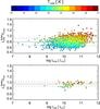 |
Fig. E.2 Top panel (bottom-panel): comparison between the ratio of LFIR ( LIR ) obtained by Sanders & Mirabel (1996) equations and with the direct integration of our final templates. The solid line shows the median value and colors represent the dust temperature (in K) of the cold component. Dashed lines represent the 1σ dispersion. |
Sanders & Mirabel (1996; hereafter SM96) show the most often used relation to obtain LFIR and LIR as a linear combination of fluxes at 12, 25, 60 and 100 μm (observed frame).
They have used the following equations: ![Mathematical equation: \appendix \setcounter{section}{5} \begin{eqnarray} \label{eq:sanders and Mirabel} && F_{\rm IR} = 1.8\times10^{-14}\left(13.48f_{12}+5.16f_{25}+2.58f_{60}+f_{100}\right)\left[{\rm W~m^{-2}}\right] \nonumber\\ && L_{\rm IR}(8{-}1000~\mu {\rm m})= 4\pi D_{\rm L}^2~F_{\rm IR}\left[\lsun\right] \nonumber \\ && F_{\rm FIR} = 1.26\times10^{-14}\left(2.58f_{60}+f_{100}\right)\left[{\rm W~m^{-2}}\right]\\ && L_{\rm FIR}(40{-}500~\mu {\rm m})= 4\pi D_{\rm L}^2CF_{\rm FIR}\left[\lsun\right],\nonumber \end{eqnarray}](/articles/aa/full_html/2017/06/aa29009-16/aa29009-16-eq345.png) (E.1)where fx is the respective IRAS flux expressed in Jy, DL is the source luminosity distance in Mpc, and C is the color correction constant normally related to the f100/f60 color, which is related to the IR peak emission.
(E.1)where fx is the respective IRAS flux expressed in Jy, DL is the source luminosity distance in Mpc, and C is the color correction constant normally related to the f100/f60 color, which is related to the IR peak emission.
Figure E.2 top panel shows the relation between the ratio of LFIR from SM96 ( ) and our LFIR values obtained from direct integration of the final SED fits. Considering a constant value of C = 1.4 (Sanders & Mirabel 1996) in SM96’s equation for LFIR , we observe an underestimation of the LFIR compared with our results. The median value of the
  /LFIR ratio is 0.8. Also, the luminosities ratio shows a dispersion strongly related to the dust temperature of the cold component. The /LFIR ratio is equal to 1 only for sources with Tcold between 24 and 26 K.
The bottom panel of Fig. E.2 shows the same comparison as the top panel but for LIR . The ratio between the result obtained from SM96 equation ( ) and our LIR has a median value of median
  with a small dispersion (σ = 0.005). However, since the SM96’s equation to obtain the total LIR needs four data points (fluxes at 12, 25, 60 and 100 μm), the number of sources is very limited (e.g., only 72 sources have LIR but 1599 have LFIR , as the SM96’s equations need only two fluxes in order to estimate LFIR .)
 |
Fig. E.3 Ratio between the LFIR (top) and LIR (bottom) from our calibration (O17) using the respective values obtained by the direct integration. The solid line is the median value and colors represent the dust temperature of the cold component. Dashed lines represent the 1σ dispersion. |
The SM96 calibration is based on the use of only IRAS fluxes (mainly at 60 and 100 μm), and a modified gray-body with β between 1 and 2. The problem is that this calibration uses the simplest dust emission model with no information at wavelengths greater than 100 μm. Thus this model has the problem that the peak emission near 100 μm is not well defined and, therefore, it is not possible to identify the position of the peak of the IR emission. Additionally, it is expected that the flux between 50 to 1000 μm contributes ~65% of LIR , implying that it is important to have information from the sub-mm. However, in general terms, the calibration showed by SM96 is an excellent first approximation of LIR (λ = 8–1000 μm) and for the far-infrared luminosity (λ = 40–500 μm). However, now we have access to a greater range of photometric measurements (with more points within this range) and the access to more detailed dust emission models, with deeper physical constrains (e.g., the DL07 models). With this idea in mind, we re-calibrate the SM96 equations and furthermore, we propose an easier and simpler linear combination of the IRAS filters in order to estimate the LIR and LFIR using only two filters (at 60 μm and 100 μm).
Our calibration is expressed by the following equations:
For FIR luminosity (40–500 μm) ![Mathematical equation: \appendix \setcounter{section}{5} \begin{eqnarray} \frac{F_{\rm FIR}}{\left[{\rm W~m^{-2}}\right]}& =& 1.26 \times 10^{-14} \left(0.752\frac{f_{60}}{\left[{\rm Jy}\right]}+3.236\frac{f_{100}}{\left[{\rm Jy}\right]}\right) \end{eqnarray}](/articles/aa/full_html/2017/06/aa29009-16/aa29009-16-eq357.png) (E.2)For total IR luminosity (8–1000 μm)
(E.2)For total IR luminosity (8–1000 μm) ![Mathematical equation: \appendix \setcounter{section}{5} \begin{eqnarray} \frac{F_{\rm IR}}{\left[{\rm W~m^{-2}}\right]} &=& 1.8\times10^{-14}\left(1.439\frac{f_{60}}{\left[{\rm Jy}\right]}+2.450\frac{f_{100}}{\left[{\rm Jy}\right]}\right) \end{eqnarray}](/articles/aa/full_html/2017/06/aa29009-16/aa29009-16-eq359.png) (E.3)where the luminosity is obtained from the conventional equation:
(E.3)where the luminosity is obtained from the conventional equation: ![Mathematical equation: \appendix \setcounter{section}{5} \begin{equation} \frac{L}{\left[\lsun\right]} = 3.13\times10^{19} \left(\frac{D_{\rm L}}{\left[{\rm Mpc}\right]}\right)^2 \frac{F}{\left[{\rm W~m^{-2}}\right]}\cdot \end{equation}](/articles/aa/full_html/2017/06/aa29009-16/aa29009-16-eq360.png) (E.4)Figure E.3 top (bottom) panel shows the ratio between the LFIR (LIR) obtained with our calibration using the values derived the direct integration of the SED templates, as a function of the LFIR (LIR) also obtained for the integration of the SED templates.
(E.4)Figure E.3 top (bottom) panel shows the ratio between the LFIR (LIR) obtained with our calibration using the values derived the direct integration of the SED templates, as a function of the LFIR (LIR) also obtained for the integration of the SED templates.
We use 1599 sources and find that the median value of the  and
and  ratios ~1.001 with standard deviation ~0.13.
One other advantage of our calibration is that these is no correlation between the dispersion and the Tcold . Furthermore, our equations do not need a temperature correction (as shown the SM96 with the C factor) to compensate for over- or underestimations.
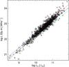 |
Fig. E.4 Correlation between the luminosity at 22 μm and the total IR luminosity. The red line shows the best fit, blue and green lines are the best-fit lines obtained by Rieke et al. (2009) and Jarrett et al. (2013), respectively, from the SFR, and the luminosity at 22 μm. Symbols represent the same sSFR as in Fig. 10 |
Another interesting way to obtain the total LIR from a single measurement comes from the use of the luminosity at 22 μm (WISE W4 filter). Using a sub-sample of 924 galaxies with at least five photometric points for a SED fitting with  , we obtain that the best fit equation is expressed by:
 ![Mathematical equation: \appendix \setcounter{section}{5} \begin{equation} \rm \frac{\lir}{[{\it L}_{\odot}]} =10^{-10.60\pm0.17} \left(\frac{{\it L}_{22~\mum}}{\rm [W~Hz^{-1}]}\right)^{0.926\pm0.008} , \end{equation}](/articles/aa/full_html/2017/06/aa29009-16/aa29009-16-eq364.png) (E.5)with rms = 0.096. The best-fit line for our data is plotted in Fig. E.4 as a red solid line. Similar relations are shown in different works, where the SFR of the galaxy is derived from the flux at 24 μm. In particular, Fig. E.4 reports two examples, one from Jarrett et al. (2013; green line) and the other from Rieke et al. (2009; blue line). The point dispersion in our calibration does not show correlations with Tcold , M∗ , or Mdust .
(E.5)with rms = 0.096. The best-fit line for our data is plotted in Fig. E.4 as a red solid line. Similar relations are shown in different works, where the SFR of the galaxy is derived from the flux at 24 μm. In particular, Fig. E.4 reports two examples, one from Jarrett et al. (2013; green line) and the other from Rieke et al. (2009; blue line). The point dispersion in our calibration does not show correlations with Tcold , M∗ , or Mdust .
 |
Fig. E.5 Correlation between total LIR and the luminosities at 550 μm (top panel) and 850 μm (bottom panel). The dust temperature (in K) of the cold component is shown by the color-scale. The blue line shows the best fit. Symbols are as shown in Fig. 10. The black cross shows the typical error. |
Finally, we find a correlation between the sub-mm fluxes (at 350 μm, 550 μm, 850 μm) and the total LIR . We present these correlations in Sect. 4.5 for the flux at 350 μm.
Figure E.5 shows the correlation between the LIR and the luminosity at 550 μm (top panel) and 850 μm (bottom panel), where the best fits (blue lines) are determined by the following equations, respectively: ![Mathematical equation: \appendix \setcounter{section}{5} \begin{eqnarray} \frac{L_{\rm IR}}{[L_{\odot}]} & = 10^{-14.588\pm0.002 }\left(\frac{L_{550}}{\rm [W~Hz^{-1}]}\right)^{1.074\pm0.005}\\ \frac{L_{\rm IR}}{[L_{\odot}]} & = 10^{-17.135\pm0.002}\left(\frac{L_{850}}{\rm [W~Hz^{-1}]}\right)^{1.221\pm0.0051}\cdot\nonumber \end{eqnarray}](/articles/aa/full_html/2017/06/aa29009-16/aa29009-16-eq366.png) (E.6)These relations show that the dispersion is related to the dust temperature of the cold component. Following the same idea of the dust plane shown in Sect. 4.5, we define a plane using the total IR luminosity, the luminosity at 550 μm (at 850 μm ), and the dust temperature of the cold component. The best fits are described as follow:
(E.6)These relations show that the dispersion is related to the dust temperature of the cold component. Following the same idea of the dust plane shown in Sect. 4.5, we define a plane using the total IR luminosity, the luminosity at 550 μm (at 850 μm ), and the dust temperature of the cold component. The best fits are described as follow: ![Mathematical equation: \appendix \setcounter{section}{5} \begin{eqnarray} \log \left(\frac{L_{\rm IR}}{ [L_{\odot}]}\right) & -& 1.00\times \log \left(\frac{L_{550}}{\rm [W~Hz^{-1}]}\right)\nonumber \\ &-&\rm 0.13\times \left(\frac{{ \it T}_{\rm cold}}{\rm [K]}\right) + 16.03 = 0 \\ \log \left(\frac{L_{\rm IR}}{[L_{\odot}]}\right) & -& 1.01\times \log \left(\frac{L_{850}}{\rm [W~Hz^{-1}]}\right)\nonumber \\ &-&\rm 0.15\times \left(\frac{{\it T}_{\rm cold}}{\rm [K]}\right) + 15.93 = 0. \nonumber \end{eqnarray}](/articles/aa/full_html/2017/06/aa29009-16/aa29009-16-eq367.png) (E.7)A similar dust plane is defined for the luminosity at 350 μm, see Sect. 4.5 for more details.
(E.7)A similar dust plane is defined for the luminosity at 350 μm, see Sect. 4.5 for more details.
Appendix F: Estimating dust masses from limited sub-mm data
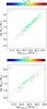 |
Fig. F.1 Relation between dust mass and the luminosities at 550 μm (top panel) and at 850 μm (bottom panel). The dust temperature (in K) of the cold component is shown by the color-scale. The blue line shows the best fit. Symbols are as shown in Fig. 14. The typical error is shown by the black cross. |
The most common approach to estimate the dust mass in a galaxy from a single measurement is using the flux at 850 μm (e.g., Dunne et al. 2000; Dunne & Eales 2001). This is because the most common approach would be to have a set of measurements, and then perform a fit according to a physical dust model. The aforementioned results were limited by the data, since at that time there were not deep measurements between 100–500 μm. In Sect. 4.5 we show a correlation between the dust mass and the luminosity at 350 μm. Now we extend this correlation to the luminosities at 550 μm and 850 μm.
Figure F.1 shows the correlations between the Mdust and the sub-mm luminosities at 550 μm (top panel) and 850 μm (bottom panel), where the color-scale shows the dust temperature of the cold component. The best fit (blue lines) equations are represented by: ![Mathematical equation: \appendix \setcounter{section}{6} \begin{eqnarray} \frac{M_{\rm dust}}{[M_{\odot}]} & =& 10^{-13.606\pm0.002}\left(\frac{L_{550}}{\rm [W~Hz^{-1}]}\right)^{0.927\pm0.05}\\ \frac{M_{\rm dust}}{[M_{\odot}]} & =& 10^{-12.84\pm0.002}\left(\frac{L_{850}}{\rm [W~Hz^{-1}]}\right)^{0.920\pm0.005}\cdot\nonumber \end{eqnarray}](/articles/aa/full_html/2017/06/aa29009-16/aa29009-16-eq368.png) (F.1)Analogously to the dust plane (Sect. 4.5), we define a plane among the luminosities in the sub-mm,the dust mass and the dust temperature of the cold component. The equations for the best fits are:
(F.1)Analogously to the dust plane (Sect. 4.5), we define a plane among the luminosities in the sub-mm,the dust mass and the dust temperature of the cold component. The equations for the best fits are: ![Mathematical equation: \appendix \setcounter{section}{6} \begin{eqnarray} \log \left(\frac{M_{\rm dust}}{[M_{\odot}]}\right) & - &0.961\times \log \left(\frac{L_{550}}{\rm [W~Hz^{-1}]}\right)\nonumber \\ &+& \rm 0.064\times \left(\frac{{\it T}_{\rm cold}}{\rm [K]}\right) + 12.933 = 0\\ \rm \log \left(\frac{{\it M}_{dust}}{[{\it M}_{\sun}]}\right) &-& \rm 0.993\times\log \left(\frac{L_{850}}{[W~Hz^{-1}]}\right) \nonumber\\ \rm &+& \rm 0.054\times \left(\frac{{\it T}_{cold}}{[K]}\right) + 13.310 = 0. \nonumber \end{eqnarray}](/articles/aa/full_html/2017/06/aa29009-16/aa29009-16-eq369.png) (F.2)These relations are independent to the sSFR classification.
(F.2)These relations are independent to the sSFR classification.
All Tables
All Figures
|
Fig. 1 An example dust-emission template from Draine & Li (2007), between 7 and 1100 μm. Overlaid are the transmission curves of all the filters used in this work: WISE W3 and W4 ; IRAS 12, 25, 60 and 100 μm; Planck 350, 550 and 850 μm and SCUBA 850 μm. |
| In the text | |
|
Fig. 2 Distribution of redshift (left) and number of photometric points per galaxy (right) for the 1630 objects in our final sample. The shaded histograms in both panels show the equivalent distributions for the subset of galaxies with CO detections. |
| In the text | |
|
Fig. 3 The histogram of the reduced χ2 |
| In the text | |
|
Fig. 4 Examples of DL07 spectral energy distribution (SED) fits to galaxies in our sample, as named in each panel. Photometric data points are shown with red circles and corresponding black error bars. Panels are organized (left to right) by the number of photometric data points (4 to 7 points). The top (bottom) row shows “normal” star forming (starburst; SB) galaxies; (see Sect. 4.3). The single best-fit DL07 template SED is shown in yellow. All SEDs which satisfy the reduced χ2 criterion (see Sect. 3) are shown in gray; the weighted geometric mean of these is used as our FTF (shown in black). The two temperature component model fits (Eq. (7)) are shown in red (cold dust component), blue (warm dust component), and green (sum of cold and warm dust components). |
| In the text | |
|
Fig. 5 Left panel: composite SEDs of galaxies with normal sSFR (875 normal star forming galaxies; red) and high sSFR (26 SB galaxies; blue), for wavelengths between 10 and 1000 μm. The orange spectrum is from a subsample (277 templates) of the normal galaxies closest to the MS (− 0.5 < sSFR [yr-1] < 0.5, see Sect. 4.3). Similarly, the purple spectrum is a subsample (11 templates) of the most extreme SB galaxies in our sample (sSFR [yr-1] > 0.8). Middle panel: comparison of composite SED of the subsample of galaxies closest to the MS (orange) with templates of Sa and Sc galaxies (black and green, respectively, obtained from the SWIRE template library, see text). Right panel: comparison of composite SED of the subsample of the most extreme SB galaxies (purple) with spectra of Arp 220 (a starburst-ULIRG; gray), IRAS 22491-1808 (a starburst-ULIRG; green), and IRAS 19254-7245 South (a Seyfert 2-starburst-ULIRG; black). In all panels, the composite spectra are plotted using solid lines, and their corresponding dispersions (± 0.7σ) are plotted using dotted lines of the same color. All SEDs are normalized to the 25 μm luminosity (νLν25 μm) in order to best contrast changes in the SED peak (~100 μm), sub-mm luminosities, and PAH emission at ~ 5 to 11 μm. Note that our fits use data between 12 μm and 850 μm. Further, our composite spectra do not include a stellar component, and thus do not match the comparison spectra below ~ 10 μm. |
| In the text | |
|
Fig. 6 Distribution of LIR (from the DL07-model-fits; top panels) and stellar mass (following Cluver et al. 2014; bottom panels) for our sample. Histograms for our full sample (black), all SBs (blue), all MS (red) and all passive galaxies (green) are shown. The bottom sub-panels show the equivalent normalized histograms. |
| In the text | |
|
Fig. 7 The star formation rate – stellar mass plane. Interacting galaxies are shown with Xs, and non-interacting galaxies (or those which we were unable to classify due to lack of deep imaging) with circles. Symbol colors indicate the CO J:1-0 luminosity, with gray denoting galaxies without global CO J:1-0 measurements. The red solid line shows the MS locus from Elbaz et al. (2011), and the red dotted line shows the MS locus from Elbaz et al. (2007). The other lines delineate the limits used to classify our sample in starburstiness: SB galaxies lie above the blue solid line; Intermediate-SB (InSB) galaxies lie between the blue solid and green dashed lines; normal star forming galaxies (MS) lie between the green dashed and the cyan dashed lines; and PAS galaxies lie below the black solid line. The typical error is shown in the bottom right corner. |
| In the text | |
|
Fig. 8 From left to right: distributions of the emissivity index (β), the temperatures of the cold (Tcold) and warm (Twarm) dust components, and the luminosity-weighted dust temperature (Tweight). In all panels, the distribution of the full sample is shown in black, SB galaxies in blue, MS galaxies in red, and PAS galaxies in green. The lower panels show the equivalent normalized histograms. |
| In the text | |
|
Fig. 9 Distribution of the DL07-model-derived dust mass. The full sample is shown in black, and the sub-samples of SB, MS, and PAS galaxies are shown with the same colors as in Fig. 8. The bottom panel shows the equivalent normalized histograms. |
| In the text | |
|
Fig. 10 Ratio of dust masses (two component fit to DL07 model fit) as a function of DL07 model fit dust masses. SBs, MS, and PAS galaxies are plotted as diamonds, squares, and crosses, respectively. Upward and downward triangles show intermediate SB and intermediate PAS sources. The line of equality (solid black line) and median ratio (dashed black line) are also shown. Symbols are colored by IR luminosity following the color-bar. |
| In the text | |
|
Fig. 11 Relationship between IR luminosity (thus SFR) and dust mass for our sample, with the symbols colored by the temperature of the cold dust component. The figure is a projection of the dust plane we find between LIR , Mdust , and Tcold . Symbols – which denote the sSFR classification of the galaxies – are the same as in Fig. 10. The black dashed lines are the fits to the LIR –Mdust plane for cold component dust temperature bins centered at (bottom to top) 20, 22, 24, 26 and 28 K. The purple line shows the relationship between LIR and Mdust obtained by da Cunha et al. (2010) where dust temperature is not taken into account. The typical error is shown in the top right of the plot. |
| In the text | |
|
Fig. 12 Left and middle panels: dependence of the dust mass and IR luminosity on the 350 μm monochromatic luminosity. Symbol colors show the temperature of the cold dust component, and the blue line shows the best fit. The typical error is shown by the black cross. Equivalent figures for monochromatic luminosities at 550 μm and 850 μm can be found in Appendices E and F. Right panel: correlation between the temperature of the cold dust component and the 100 μm to 350 μm flux ratio, with the best fit shown by the dashed blue line. Large, red crosses show the mean value of Tcold in 0.5 mag color bins, and the red dashed curve corresponds to the best fit line to the red crosses. The typical error in the x-axis is shown by the black horizontal line. Similar plots relating Tcold to IR and sub-mm colors can be found in Appendix D. In all panels the symbols are the same as in Fig. 10. |
| In the text | |
|
Fig. 13 Top panel: dust to stellar mass ratio ( |
| In the text | |
|
Fig. 14 Relationships between dust mass and atomic gas mass (left), molecular gas mass (middle) and total ISM mass (right). Black symbols are used for galaxies with HI and CO observations and dust mass from DL07 models; red symbols are used for galaxies with HI and CO observations, but with dust masses estimated from the luminosity at 350, 550 or 850 μm (see Eq. (16) and Appendix F); Gray symbols denote galaxies with either HI or CO observations and dust mass from DL07 models. The solid black lines in each panel show the best fit to all sources with measurements of both MHI and Mmol, and the gray dashed lines in the two left panels show the fit to all points in the respective panel. The typical error is shown by the black cross in each panel. |
| In the text | |
|
Fig. 15 Dust to ISM mass ratio as a function of stellar mass. Symbols are the same as in Fig. 10 and colors represent the gas fraction. The black solid and dashed lines show the median and mean dust to gas ratios, respectively, for the entire sample. Colored solid lines show median values for SB (blue), MS (red), and PAS (green) galaxies. The black cross shows the typical error. |
| In the text | |
|
Fig. 16 A comparison of the temperature of the cold dust component (Tcold; from the two component fit) and the luminosity weighted temperature (Tweight) for our sample. The different symbols show SBs (diamonds), MS (squares), PAS (crosses), intermediate SB (upward triangles) and intermediate PAS (downward triangles) galaxies. Symbols are color-coded by the temperature of the warm dust component following the color bar. The dashed and solid lines show the best fit and the line of equality, respectively. |
| In the text | |
|
Fig. 17 Atomic hydrogen mass (left), |
| In the text | |
|
Fig. 18 Ratio of the monochromatic luminosity at 850 μm to the ISM mass as a function of monochromatic luminosity at 850 μm. Circles show galaxies of our sample and large triangles show galaxies from Scoville et al. (2014). Symbols are colored by the LIR following the color bar. The median value for our sample is shown by the dashed line, while dotted lines show the median values obtained by Scoville et al. (2014) and by Hughes et al. (2017). The black cross shows the typical error. |
| In the text | |
|
Fig. A.1 Normalized distributions of the dust-mass fraction heated by PDRs (γ; top panel), the constant intensity of the radiation field (Umin; middle) and the polycyclic aromatic hydrocarbon index (qPAH; bottom) of the DL07 templates used in our sample. Histograms show the distribution of the full sample (black), SB (blue), MS (red), and PAS (green) galaxies. In the bottom panel the qpah histogram is divided in three groups of values, shown by the purple solid and black dashed lines: Milky Way models (left side of the solid line), the Large Magellanic Cloud (between purple solid and black dashed lines), and the Small Magellanic Cloud (right side of the black dashed line). |
| In the text | |
|
Fig. C.1 Comparison between stellar mass estimates and the ratio between the NASA Sloan Atlas estimation (top), the (Chang et al. 2015) estimation (middle) and the MPA-JHU estimation (bottom) with our stellar mass. The solid line shows the median value and dashed lines show the ± 1σ dispersion. Colors represent the apparent diameter of the galaxies in arcminutes. Crosses show sources classified as interacting galaxies and circles show non-interacting galaxies. |
| In the text | |
|
Fig. D.1 Relation between IR and sub-mm colors (with exception of the first panel, which is the color f60/f100) and the dust temperature of the cold component (fλ, λ in μm). This relation is shown only for galaxies with five or more photometric measurements and |
| In the text | |
|
Fig. D.2 As in Fig. D.1, but for the IR flux at 22 μm (top) and at 12 μm (bottom) and the light-weighted dust temperature. |
| In the text | |
|
Fig. E.1 Ratio of LIR /LFIR as a function of LIR . Circles show non-interacting galaxies and crosses show interacting galaxies. The median ratio for the sample is 1.20 (solid black line). The dashed lines show the 1σ dispersion. |
| In the text | |
|
Fig. E.2 Top panel (bottom-panel): comparison between the ratio of LFIR ( LIR ) obtained by Sanders & Mirabel (1996) equations and with the direct integration of our final templates. The solid line shows the median value and colors represent the dust temperature (in K) of the cold component. Dashed lines represent the 1σ dispersion. |
| In the text | |
|
Fig. E.3 Ratio between the LFIR (top) and LIR (bottom) from our calibration (O17) using the respective values obtained by the direct integration. The solid line is the median value and colors represent the dust temperature of the cold component. Dashed lines represent the 1σ dispersion. |
| In the text | |
|
Fig. E.4 Correlation between the luminosity at 22 μm and the total IR luminosity. The red line shows the best fit, blue and green lines are the best-fit lines obtained by Rieke et al. (2009) and Jarrett et al. (2013), respectively, from the SFR, and the luminosity at 22 μm. Symbols represent the same sSFR as in Fig. 10 |
| In the text | |
|
Fig. E.5 Correlation between total LIR and the luminosities at 550 μm (top panel) and 850 μm (bottom panel). The dust temperature (in K) of the cold component is shown by the color-scale. The blue line shows the best fit. Symbols are as shown in Fig. 10. The black cross shows the typical error. |
| In the text | |
|
Fig. F.1 Relation between dust mass and the luminosities at 550 μm (top panel) and at 850 μm (bottom panel). The dust temperature (in K) of the cold component is shown by the color-scale. The blue line shows the best fit. Symbols are as shown in Fig. 14. The typical error is shown by the black cross. |
| In the text | |
Current usage metrics show cumulative count of Article Views (full-text article views including HTML views, PDF and ePub downloads, according to the available data) and Abstracts Views on Vision4Press platform.
Data correspond to usage on the plateform after 2015. The current usage metrics is available 48-96 hours after online publication and is updated daily on week days.
Initial download of the metrics may take a while.