| Issue |
A&A
Volume 586, February 2016
|
|
|---|---|---|
| Article Number | A132 | |
| Number of page(s) | 26 | |
| Section | Interstellar and circumstellar matter | |
| DOI | https://doi.org/10.1051/0004-6361/201424945 | |
| Published online | 09 February 2016 | |
Planck intermediate results
XXIX. All-sky dust modelling with Planck, IRAS, and WISE observations
1
APC, AstroParticule et Cosmologie, Université Paris Diderot,
CNRS/IN2P3, CEA/lrfu, Observatoire de Paris, Sorbonne Paris Cité, 10 rue Alice Domon et Léonie
Duquet, 75205
Paris Cedex 13,
France
2
African Institute for Mathematical Sciences,
6-8 Melrose Road, Muizenberg,
7945
Cape Town, South
Africa
3
Agenzia Spaziale Italiana Science Data Center, via del Politecnico
snc, 00133
Roma,
Italy
4
Agenzia Spaziale Italiana, Viale Liegi 26,
00133
Roma,
Italy
5
Astrophysics Group, Cavendish Laboratory, University of
Cambridge, J J Thomson
Avenue, Cambridge
CB3 0HE,
UK
6
Astrophysics & Cosmology Research Unit, School of
Mathematics, Statistics & Computer Science, University of
KwaZulu-Natal, Westville Campus,
Private Bag X54001, 4000
Durban, South
Africa
7
Atacama Large Millimeter/submillimeter Array, ALMA Santiago
Central Offices, Alonso de Cordova 3107, Vitacura, Casilla 763 0355,
Santiago,
Chile
8
CITA, University of Toronto, 60 St. George St., Toronto, ON
M5S 3H8,
Canada
9
CNRS, IRAP, 9
Av. colonel Roche, BP
44346, 31028
Toulouse Cedex 4,
France
10
California Institute of Technology, Pasadena, California, USA
11
Centro de Estudios de Física del Cosmos de Aragón (CEFCA), Plaza
San Juan, 1, planta 2, 44001
Teruel,
Spain
12
Computational Cosmology Center, Lawrence Berkeley National
Laboratory, Berkeley,
California,
USA
13
Consejo Superior de Investigaciones Científicas
(CSIC), Madrid,
Spain
14
DSM/Irfu/SPP, CEA-Saclay, 91191
Gif-sur-Yvette Cedex,
France
15
DTUSpace, National Space Institute, Technical University of
Denmark, Elektrovej
327, 2800
Kgs. Lyngby,
Denmark
16
Département de Physique Théorique, Université de
Genève, 24 Quai E.
Ansermet, 1211
Genève 4,
Switzerland
17
Departamento de Física, Universidad de Oviedo,
Avda. Calvo Sotelo s/n,
Oviedo,
Spain
18
Department of Astrophysics/IMAPP, Radboud University
Nijmegen, PO Box
9010, 6500 GL
Nijmegen, The
Netherlands
19
Department of Physics & Astronomy, University of British
Columbia, 6224 Agricultural Road,
Vancouver, British
Columbia, Canada
20
Department of Physics and Astronomy, Dana and David Dornsife
College of Letter, Arts and Sciences, University of Southern California,
Los Angeles, CA
90089,
USA
21
Department of Physics and Astronomy, University College
London, London
WC1E 6BT,
UK
22
Department of Physics, Florida State University,
Keen Physics Building, 77 Chieftan
Way, Tallahassee,
Florida,
USA
23
Department of Physics, Gustaf Hällströmin katu 2a, University of
Helsinki, 00014
Helsinki,
Finland
24
Department of Physics, Princeton University,
Princeton, New Jersey, USA
25
Department of Physics, University of California,
Santa Barbara, California, USA
26
Department of Physics, University of Illinois at
Urbana-Champaign, 1110 West Green
Street, Urbana,
Illinois,
USA
27
Dipartimento di Fisica e Astronomia G. Galilei, Università degli
Studi di Padova, via Marzolo
8, 35131
Padova,
Italy
28
Dipartimento di Fisica e Scienze della Terra, Università di
Ferrara, via Saragat
1, 44122
Ferrara,
Italy
29
Dipartimento di Fisica, Università La Sapienza,
P.le A. Moro 2, 00133
Roma,
Italy
30
Dipartimento di Fisica, Università degli Studi di
Milano, via Celoria,
16, 20133
Milano,
Italy
31
Dipartimento di Fisica, Università degli Studi di
Trieste, via A. Valerio
2, 34127
Trieste,
Italy
32
Dipartimento di Fisica, Università di Roma Tor
Vergata, via della Ricerca
Scientifica, 1, 00185
Roma,
Italy
33
Discovery Center, Niels Bohr Institute,
Blegdamsvej 17, 1165
Copenhagen,
Denmark
34
Dpto. Astrofísica, Universidad de La Laguna (ULL),
38206 La Laguna, Tenerife, Spain
35
European Southern Observatory, ESO Vitacura, Alonso de Cordova 3107, Vitacura, Casilla
19001, Santiago,
Chile
36
European Space Agency, ESAC, Planck Science Office, Camino bajo
del Castillo, s/n, Urbanización Villafranca del Castillo, Villanueva de la
Cañada, Madrid,
Spain
37
European Space Agency, ESTEC, Keplerlaan 1,
2201 AZ
Noordwijk, The
Netherlands
38 Facoltà di Ingegneria, Università degli Studi e-Campus, via
Isimbardi 10, 22060 Novedrate ( CO), Italy
39
HGSFP and University of Heidelberg, Theoretical Physics
Department, Philosophenweg
16, 69120
Heidelberg,
Germany
40
Helsinki Institute of Physics, Gustaf Hällströmin katu 2,
University of Helsinki, Helsinki, Finland
41
INAF−Osservatorio
Astrofisico di Catania, via S. Sofia 78, Catania, Italy
42
INAF−Osservatorio
Astronomico di Padova, Vicolo dell’Osservatorio 5, 35131
Padova,
Italy
43
INAF−Osservatorio
Astronomico di Roma, via di Frascati 33, Monte Porzio Catone,
Italy
44
INAF−Osservatorio
Astronomico di Trieste, via G.B. Tiepolo 11, 34131
Trieste,
Italy
45
INAF/IASF Bologna, via Gobetti 101, 40127
Bologna,
Italy
46
INAF/IASF Milano, via E. Bassini 15, 20133
Milano,
Italy
47
INFN, Sezione di Bologna, via Irnerio 46,
40126
Bologna,
Italy
48
INFN, Sezione di Roma 1, Università di Roma
Sapienza, Piazzale Aldo Moro
2, 00185
Roma,
Italy
49
INFN/National Institute for Nuclear Physics,
via Valerio 2, 34127
Trieste,
Italy
50
IPAG: Institut de Planétologie et d’Astrophysique de Grenoble,
Université Grenoble Alpes, IPAG, CNRS, IPAG, 38000
Grenoble,
France
51
Imperial College London, Astrophysics group, Blackett
Laboratory, Prince Consort
Road, London,
SW7 2AZ,
UK
52
Infrared Processing and Analysis Center, California Institute of
Technology, Pasadena,
CA
91125,
USA
53
Institut Universitaire de France, 103, bd Saint-Michel, 75005
Paris,
France
54
Institut d’Astrophysique Spatiale, CNRS (UMR 8617) Université
Paris-Sud 11, Bâtiment
121, 91898
Orsay,
France
55
Institut d’Astrophysique de Paris, CNRS (UMR 7095),
98bis Boulevard Arago,
75014
Paris,
France
56
Institute for Space Sciences, Bucharest-Magurale,
Romania
57
Institute of Astronomy, University of Cambridge,
Madingley Road, Cambridge
CB3 0HA,
UK
58
Institute of Theoretical Astrophysics,University of
Oslo, Blindern,
0371
Oslo,
Norway
59
Instituto de Astrofísica de Canarias, C/Vía Láctea s/n, La Laguna, 38200
Tenerife,
Spain
60
Instituto de Física de Cantabria (CSIC-Universidad de
Cantabria), Avda. de los Castros
s/n, 39005
Santander,
Spain
61
Jet Propulsion Laboratory, California Institute of
Technology, 4800 Oak Grove
Drive, Pasadena,
California,
USA
62
Jodrell Bank Centre for Astrophysics, Alan Turing Building, School
of Physics and Astronomy, The University of Manchester, Oxford Road, Manchester, M13
9PL, UK
63
Kavli Institute for Cosmology Cambridge,
Madingley Road, Cambridge, CB3 0HA, UK
64
LAL, Université Paris-Sud, CNRS/IN2P3,
91898
Orsay,
France
65
LERMA, CNRS, Observatoire de Paris, 61 Avenue de
l’Observatoire, 75000
Paris,
France
66
Laboratoire AIM, IRFU/Service d’Astrophysique−CEA/DSM−CNRS −
Université Paris Diderot, Bât. 709, CEA-Saclay, 91191
Gif-sur-Yvette Cedex,
France
67
Laboratoire Traitement et Communication de l’Information, CNRS
(UMR 5141) and Télécom ParisTech, 46 rue Barrault, 75634
Paris Cedex 13,
France
68
Laboratoire de Physique Subatomique et de Cosmologie, Université
Joseph Fourier Grenoble I, CNRS/IN2P3, Institut National Polytechnique de
Grenoble, 53 rue des
Martyrs, 38026
Grenoble Cedex,
France
69
Laboratoire de Physique Théorique, Université Paris-Sud 11
& CNRS, Bâtiment
210, 91405
Orsay,
France
70
Lawrence Berkeley National Laboratory,
Berkeley, California, USA
71
Max-Planck-Institut für Astrophysik, Karl-Schwarzschild-Str. 1, 85741
Garching,
Germany
72
McGill Physics, Ernest Rutherford Physics Building, McGill
University, 3600 rue University, Montréal, QC,
H3A 2T8,
Canada
73
National University of Ireland, Department of Experimental
Physics, Maynooth,
Co. Kildare,
Ireland
74
Niels Bohr Institute, Blegdamsvej 17, Copenhagen, Denmark
75
Observational Cosmology, Mail Stop 367-17, California Institute of
Technology, Pasadena,
CA, 91125, USA
76
Princeton University Observatory, Peyton Hall, Princeton, NJ
08544-1001,
USA
77
SISSA, Astrophysics Sector, via Bonomea 265,
34136
Trieste,
Italy
78
School of Physics and Astronomy, Cardiff University,
Queens Buildings, The Parade,
Cardiff, CF24 3AA, UK
79
Space Research Institute (IKI), Russian Academy of
Sciences, Profsoyuznaya Str,
84/32, 117997
Moscow,
Russia
80
Space Sciences Laboratory, University of California,
Berkeley, California, USA
81
Special Astrophysical Observatory, Russian Academy of
Sciences, Nizhnij Arkhyz,
Zelenchukskiy region, 369167
Karachai-Cherkessian Republic,
Russia
82
Sub-Department of Astrophysics, University of
Oxford, Keble Road,
Oxford
OX1 3RH,
UK
83
UPMC Univ Paris 06, UMR7095, 98bis Boulevard Arago, 75014
Paris,
France
84
Université de Toulouse, UPS-OMP, IRAP, 31028
Toulouse Cedex 4,
France
85
Universities Space Research Association, Stratospheric Observatory
for Infrared Astronomy, MS
232-11, Moffett
Field, CA
94035,
USA
86
University of Granada, Departamento de Física Teórica y del
Cosmos, Facultad de Ciencias, 18071
Granada,
Spain
87
University of Granada, Instituto Carlos I de Física Teórica y
Computacional, 18071
Granada,
Spain
88
Warsaw University Observatory, Aleje Ujazdowskie 4, 00-478
Warszawa,
Poland
Received: 8 September 2014
Accepted: 14 December 2015
Abstract
We present all-sky modelling of the high resolution Planck, IRAS, and WISE infrared (IR) observations using the physical dust model presented by Draine & Li in 2007 (DL, ApJ, 657, 810). We study the performance and results of this model, and discuss implications for future dust modelling. The present work extends the DL dust modelling carried out on nearby galaxies using Herschel and Spitzer data to Galactic dust emission. We employ the DL dust model to generate maps of the dust mass surface density ΣMd, the dust optical extinction AV, and the starlight intensity heating the bulk of the dust, parametrized by Umin. The DL model reproduces the observed spectral energy distribution (SED) satisfactorily over most of the sky, with small deviations in the inner Galactic disk and in low ecliptic latitude areas, presumably due to zodiacal light contamination. In the Andromeda galaxy (M31), the present dust mass estimates agree remarkably well (within 10%) with DL estimates based on independent Spitzer and Herschel data. We compare the DL optical extinction AV for the diffuse interstellar medium (ISM) with optical estimates for approximately 2 × 10⁵ quasi-stellar objects (QSOs) observed inthe Sloan Digital Sky Survey (SDSS). The DL AV estimates are larger than those determined towards QSOs by a factor of about 2, which depends on Umin. The DL fitting parameter Umin, effectively determined by the wavelength where the SED peaks, appears to trace variations in the far-IR opacity of the dust grains per unit AV, and not only in the starlight intensity. These results show that some of the physical assumptions of the DL model will need to be revised. To circumvent the model deficiency, we propose an empirical renormalization of the DL AV estimate, dependent of Umin, which compensates for the systematic differences found with QSO observations. This renormalization, made to match the AV estimates towards QSOs, also brings into agreement the DL AV estimates with those derived for molecular clouds from the near-IR colours of stars in the 2 micron all sky survey (2MASS). The DL model and the QSOs data are also used to compress the spectral information in the Planck and IRAS observations for the diffuse ISM to a family of 20 SEDs normalized per AV, parameterized by Umin, which may be used to test and empirically calibrate dust models. The family of SEDs and the maps generated with the DL model are made public in the Planck Legacy Archive.
Key words: dust, extinction / ISM: general
Corresponding authors: e-mail: This email address is being protected from spambots. You need JavaScript enabled to view it. ; This email address is being protected from spambots. You need JavaScript enabled to view it.
© ESO, 2016
1. Introduction
Studying the interstellar medium (ISM) is important in a wide range of astronomical disciplines, from star and planet formation to galaxy evolution. Dust changes the appearance of galaxies by absorbing ultraviolet (UV), optical, and infrared (IR) starlight, and emitting mid-IR and far-IR (FIR) radiation. Dust is an important agent in the chemical and thermodynamical evolution of the ISM. Physical models of interstellar dust that have been developed are constrained by such observations. In the present work, we study the ability of a physical dust model to reproduce IR emission and optical extinction observations, using the newly available Planck1 data.
The Planck data provide a full-sky view of the Milky Way (MW) at submillimetre (submm) wavelengths, with much higher angular resolution than earlier maps made by the Diffuse Infrared Background Experiment (DIRBE; Silverberg et al. 1993) on the Cosmic background explorer (COBE) spacecraft (Boggess et al. 1992). These new constraints on the spectral energy distribution (SED) emission of large dust grains were modelled by Planck Collaboration XI (2014, hereafter Pl using a modified blackbody (MBB) spectral model, parameterized by optical depth and dust temperature. That study, along with previous Planck results, confirmed spatial changes in the dust submm opacity even in the high latitude sky (Planck Collaboration XXIV 2011; Planck Collaboration Int. XVII 2014). The dust temperature, which reflects the thermal equilibrium, is anti-correlated with the FIR opacity. The dust temperature is also affected by the strength of the interstellar radiation field (ISRF) heating the dust. The bolometric emission per H atom is almost constant at high latitude, consistent with a uniform ISRF, but over the full sky, covering lines of sight through the Galaxy, the ISRF certainly changes. The all-sky submm dust optical depth was also calibrated in terms of optical extinction. However, no attempt was made to connect these data with a self-consistent dust model, which is the goal of this complementary paper.
Several authors have modelled the dust absorption and emission in the diffuse ISM, e.g. Draine & Lee (1984), Desert et al. (1990), Dwek (1998), Zubko et al. (2004), Compiègne et al. (2011), Jones et al. (2013), Siebenmorgen et al. (2014). We focus on one of the most widely used dust models presented by Draine & Li (2007, hereafter DL). Earlier, Draine & Lee (1984) studied the optical properties of graphite and silicate dust grains, while Weingartner & Draine (2001) and Li & Draine (2001) developed a carbonaceous-silicate grain model that has been quite successful in reproducing observed interstellar extinction, scattering, and IR emission. DL presented an updated physical dust model, extensively used to model starlight absorption and IR emission. The DL dust model employs a mixture of amorphous silicate grains and carbonaceous grains. The grains are assumed to be heated by a distribution of starlight intensities. The model assumes optical properties of the dust grains and the model SEDs are computed from first principles.
The DL model has been successfully employed to study the ISM in a variety of galaxies. Draine et al. (2007) employed DL to estimate the dust masses, abundances of polycyclic aromatic hydrocarbon (PAH) molecules, and starlight intensities in the Spitzer Infrared Nearby Galaxies Survey – Physics of the Star-Forming ISM and Galaxy Evolution (SINGS, Kennicutt et al. 2003) galaxy sample. This survey observed a sample of 75 nearby (within 30 Mpc of the Galaxy) galaxies, covering the full range in a three-dimensional parameter space of physical properties, with the Spitzer Space Telescope (Werner et al. 2004). The Key Insights on Nearby Galaxies: a FIR Survey with Herschel (KINGFISH, Kennicutt et al. 2011) project, additionally observed a subsample of 61 of the SINGS galaxies with the Herschel Space Observatory (Pilbratt et al. 2010). Aniano et al. (2012) presented a detailed resolved study of two KINGFISH galaxies, NGC 628 and NGC 6946, using the DL model constrained by Spitzer and Herschel photometry. Aniano et al. (in prep.) extended the preceding study to the full KINGFISH sample of galaxies. Draine et al. (2014, hereafter DA14), presented a resolved study of the nearby Andromeda galaxy (M31), where high spatial resolution can be achieved. The DL model proved able to reproduce the observed emission from dust in the KINGFISH galaxies and M31. Ciesla et al. (2014) used the DL model to fit the volume limited, K-band selected sample of galaxies of the Herschel Reference Survey (Boselli et al. 2010), finding it systematically underestimated the 500 μm photometry.
The new Planck all-sky maps, combined with ancillary Infrared Astronomical Satellite (IRAS, Neugebauer et al. 1984) and Wide-field Infrared Survey Explorer (WISE, Wright et al. 2010) maps allow us to explore the dust thermal emission from the MW ISM with greater spatial resolution and frequency coverage than ever before. Here we test the compatibility of the DL dust model with these new observations.
We employ WISE 122 (12 μm), IRAS 60 (60 μm), IRAS 100 (100 μm), Planck 857 (350 μm), Planck 545 (550 μm), and Planck 353 (850 μm) maps to constrain the dust emission SED in the range 10 μm <λ< 970 μm. These data allow us to generate reliable maps of the dust emission using a Gaussian point spread function (PSF) with 5′ full width at half maximum (FWHM). Working at lower resolution (1° FWHM), we can add the DIRBE 140 and DIRBE 240 photometric constraints.
We employ the DL dust model to characterize:
-
the dust mass surface density ΣMd;
-
the dust optical extinction AV;
-
the dust mass fraction in small PAH grains qPAH;
-
the fraction of the total luminosity radiated by dust that arises from dust heated by intense radiation fields, fPDR;
-
the starlight intensity Umin heating the bulk of the dust.
The estimated dust parameters for M31 are compared with those derived using the independent maps in DA14.
We compare the DL optical extinction estimates with those of Pl-MBB. We further compare the DL model reddening estimates with near-IR reddening estimates from quasi-stellar objects (QSOs) from the Sloan Digital Sky Survey (SDSS, York et al. 2000), and from stellar reddening maps in dark clouds obtained from the Two Micron All Sky Survey (2MASS, Skrutskie et al. 2006). These reveal significant discrepancies that call for a revision of the DL model. We find an empirical parameterization that renormalizes the current DL model and provides insight into what is being compensated for through the renormalization.
We use the DL model parameter Umin to bin the Planck and IRAS data for the diffuse ISM and compress the spectral information to a family of 20 dust SEDs, normalized per AV, which may be used to test and empirically calibrate dust models. We also provide the Planck 217 (1.38 mm) and Planck 143 (2.10 mm) photometric constraints, which are not used in the current dust modelling.
This paper is organized as follows. We describe the data sets in Sect. 2. In Sect. 3, we present the DL dust model, the model parametrization and the method we use to fit the model to the data. The model results are described in Sect. 4. We present the maps of the model parameters (Sect. 4.1), analyse the model ability to fit the data (Sect. 4.2) and assess the robustness of our determination of the dust mass surface density (Sect. 4.3). We compare the dust AV estimates with the MBB all-sky modelling results from Pl-MBB in Sect. 5. In Sect. 6 we propose an empirical correction to the DL AV estimates based on the comparison with QSO SDSS data. The DL model is used to compress the Planck and IRAS data into a family of 20 dust SEDs that account for the main variations of the dust emission properties in the diffuse ISM (Sect. 7). In Sect. 8, we extend our assessment of the DL AV map to molecular clouds. The difference between AV derived from the DL model and optical observations is related to dust emission properties and their evolution within the ISM in Sect. 9. We conclude in Sect. 10. The paper has four appendices. In Appendix A, we compare our analysis of Planck and IRAS observations of M31 with earlier DL modelling of Herschel and Spitzer data. In Appendix B, we detail how we estimate AV towards QSOs observed with SDSS. In Appendix C, we analyse the impact of cosmic infrared background (CIB) anisotropies in our dust modelling. In Appendix D, we describe the data products made public in the Planck Legacy Archive.
2. Data sets
We use the full mission maps of the high frequency instrument of Planck that were made public in February 2015 (Planck Collaboration I 2015; Planck Collaboration VIII 2015). The zodiacal light has been estimated and removed from the maps (Planck Collaboration XIV 2014). We remove the cosmic microwave background, as estimated with the SMICA algorithm (Planck Collaboration IX 2015), from each Planck map. Following Pl-MBB we do not remove the CO(3-2) contribution to the Planck 353 GHz band3.
A constant offset (listed in the column marked removed CIB monopole of Table 1) was added to the maps by the Planck team to account for the CIB in extragalactic studies, and we proceed to subtract it. Since the Planck team calibrated the zero-level of the Galactic emission before the zodiacal light was removed, an additional offset correction is necessary. To determine this (small) offset, we proceed exactly as in Sect. 5 of Planck Collaboration VIII (2014) by correlating the Planck 857 GHz map to the Leiden/Argentine/Bonn Survey of Galactic H i, and then cross-correlating each of the lower frequency Planck maps to the 857 GHz map, over the most diffuse areas at high Galactic latitude. These offsets make the intercepts of the linear regressions between the Planck and H i emission equal to zero emission for a zero H i column density. We note that we did not attempt to correct the Planck maps for a potential residual of the CMB dipole as done by Pl-MBB. This is not crucial for our study because we do not use microwave frequencies for fitting the DL model.
We complement the Planck maps with IRAS 60 and IRAS 100 maps. We employ the IRAS 100 map presented in Pl-MBB. It combines the small scale (<30′) features of the map presented by the Improved reprocessing of the IRAS survey (IRIS, Miville-Deschênes & Lagache 2005), and the large scale (>30′) features of the map presented by Schlegel et al. (1998, hereafter SFD). The zodiacal light emission has been estimated and removed from the SFD map, and therefore it is removed from the map we are employing4. We employ the IRAS 60 map presented by the IRIS team, with a custom estimation and removal of the zodiacal light5. The zero level of the IRAS maps is adjusted so it is consistent with the Planck 857 GHz map.
In Sects. 5 and 9.1, we compare our work with the MBB all-sky modelling results from Pl-MBB. To perform a consistent comparison, in these sections we use the same Planck and IRAS data as in Pl-MBB, i.e. the nominal mission Planck maps corrected for zodiacal light (Planck Collaboration I 2014) with the monopole and dipole corrections estimated by Pl-MBB.
WISE mapped the sky at 3.4, 4.6, 12, and 22 μm. Meisner & Finkbeiner (2014) presented a reprocessing of the entire WISE 12 μm imaging data set, generating a high resolution, full-sky map that is free of compact sources and was cleaned from several contaminating artefacts. The zodiacal light contribution was subtracted from the WISE map assuming that on spatial scales larger than 2° the dust emission at 12 μm is proportional to that in the Planck 857 GHz band. This effectively removes the zodiacal emission but at the cost of losing information on the ratio between WISE and Planck maps on scales larger than 2°. About 18% of the WISE map is contaminated by the Moon or other solar system objects. Aniano (A15, priv. comm.) prepared a new WISE map, with an improved correction of the contaminated area, which we use in this paper.
For typical lines of sight in the diffuse ISM, the dust SED peaks in the λ = 100−160 μm range. DIRBE produced low resolution (FWHM = 42′) all-sky maps at 140 and 240 μm, which can be used to test the robustness of our modelling. Additionally, we perform a lower resolution (1° FWHM) modelling, including the DIRBE 140 and DIRBE 240 photometric constraints. We use the DIRBE zodiacal light-subtracted mission average (ZSMA) maps. This modelling allows us to evaluate the importance of adding photometric constraints near the dust SED peak, which are absent in the Planck and IRAS data.
The FIS instrument (Kawada et al. 2007) on board the AKARI spacecraft (Murakami et al. 2007) observed the sky at four FIR bands in the 50−180 μm range. Unfortunately, AKARI maps were made public (Doi et al. 2015) after this paper was submitted. Moreover, the way their mosaic tiles are chosen and significant mismatch of the zero level of the Galactic emission among the tiles prevent a straightforward integration of the AKARI data into the present modeling.
Description of the data used.
All maps were convolved to yield a Gaussian PSF, with  , slightly broader than all the native resolution of the Planck maps. We use the Hierarchical Equal Area isoLatitude Pixelization (HEALPix) of a sphere coordinates (Górski et al. 2005)6. We work at resolution Nside = 2 048, so the maps have a total of 12 × 2 048 × 2 048 = 50 331 648 pixels. Each pixel is a quadrilateral of area 2.94 arcmin2 (i.e. about 1.′7 on a side). All maps and results presented in the current paper are performed using this resolution, except those of Sects. 4.3.2 and 7. The most relevant information on the data sets that are used is presented in Table 1. The amplitudes of the CIB anisotropies (CIBA) depend on the angular scale; the values listed in Table 1 are for the 5′ resolution of our data modelling.
3. The DL model
The DL dust model is a physical approach to modelling dust. It assumes that the dust consists of a mixture of amorphous silicate grains and carbonaceous grains heated by a distribution of starlight intensities. We employ the Milky Way grain size distributions (Weingartner & Draine 2001), chosen to reproduce the wavelength dependence of the average interstellar extinction within the solar neighbourhood. The silicate and carbonaceous content of the dust grains has been constrained by observations of the gas phase depletions in the ISM. The carbonaceous grains are assumed to have the properties of PAH molecules or clusters when the number of carbon atoms per grain NC ≲ 105, but to have the properties of graphite when NC ≫ 105. DL describes the detailed computation of the model SED, and AD12 describes its use in modelling resolved dust emission.
3.1. Parameterization
The IR emission of the DL dust model is parametrized by six parameters, ΣMd,qPAH,Umin,Umax,α, and γ. The definition of these parameters is now reviewed. The model IR emission is proportional to the dust mass surface density ΣMd. The PAH abundance is measured by the parameter qPAH, defined to be the fraction of the total grain mass contributed by PAHs containing NC< 103 C atoms7. As a result of single-photon heating, the tiny PAHs contributing to qPAH radiate primarily at λ< 30 μm , and this fraction is constrained by the WISE 12 band. Weingartner & Draine (2001) computed different grain size distributions for dust grains in the diffuse ISM of the MW, which are used in DL. The models in this MW3.1 series are all consistent with the average interstellar extinction law8, but have different PAH abundances in the range 0.0047 ≤ qPAH ≤ 0.047. Draine et al. (2007) found that the SINGS galaxies span the full range of qPAH models computed, with a median value of qPAH = 0.034. Models are further extrapolated into a (uniformly sampled) qPAH grid, using δqPAH = 0.001 intervals in the range 0 ≤ qPAH ≤ 0.10, as described by AD12.
Each dust grain is assumed to be heated by radiation with an energy density per unit frequency 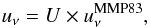 (1)where U is a dimensionless scaling factor and
  is the ISRF estimated by Mathis et al. (1983) for the solar neighbourhood. A fraction (1 − γ) of the dust mass is assumed to be heated by starlight with a single intensity U = Umin, and the remaining fraction γ of the dust mass is exposed to a power-law distribution of starlight intensities between Umin and Umax, with dM/ dU ∝ U− α. From now on, we call these the diffuse cloud and photodissociation regions (PDR) components respectively. AD12 found that the observed SEDs in the NGC 628 and NGC 6946 galaxies are consistent with DL models with Umax = 107. Given the limited number of photometric constraints, we fix the values of Umax = 107 and α = 2 to typical values found in AD12. The DL models presented in DL07 are further interpolated into a (finely sampled) Umin grid using δUmin = 0.01 intervals, as described by A15.
Therefore, in the present work the DL parameter grid has only four dimensions, ΣMd,qPAH,Umin, and γ. We explore the ranges 0.00 ≤ qPAH ≤ 0.10, 0.01 ≤ Umin ≤ 30, and 0 ≤ γ ≤ 1.0. For this range of parameters, we build a DL model library that contains the model SED in a finely-spaced wavelength grid for 1 μm <λ< 1cm.
As a derived parameter, we define the ratio 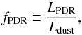 (2)where LPDR is the luminosity radiated by dust in regions where U> 102 and Ldust is the total power radiated by the dust. Clearly, fPDR depends on the fitting parameter γ in the numerator and, through the denominator, also depends on Umin. Dust heated with U> 102 emits predominantly in the λ< 100 μm range; therefore, the IRAS 60 to IRAS 100 intensity ratio can be increased to very high values by taking fPDR → 1. Conversely, for a given Umin, the minimum IRAS 60/IRAS 100 intensity ratio corresponds to models with fPDR = 0.
Another derived quantity, the mass-weighted mean starlight heating intensity ⟨ U ⟩, for α = 2, is given by 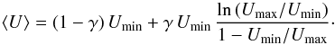 (3)Adopting the updated carbonaceous and astrosilicate densities recommended by DA14, the DL model used here is consistent with the MW ratio of visual extinction to H column density, AV/NH = 5.34 × 10⁻²² mag cm2 (i.e. NH/E(B − V) = 5.8 × 1021 cm-2 mag-1, Bohlin et al. 1978), for a dust to H mass ratio ΣMd/NHmH = 0.0091. From the dust surface density, we infer the model estimate of the visual extinction
 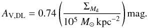 (4)
(4)
3.2. Fitting strategy and implementation
For each individual pixel, we find the DL parameters { ΣMd,qPAH,Umin,γ } that minimize ![Mathematical equation: \begin{equation} \label{eq:chi2} \chi^2 \equiv \sum_{k} \frac{[S_{{\rm obs}}(\lambda_k) -S_{{\rm DL}}(\lambda_k)]^2} {\sigma_{\lambda_k}^2} , \end{equation}](/articles/aa/full_html/2016/02/aa24945-14/aa24945-14-eq71.png) (5)where Sobs(λk) is the observed flux density per pixel, SDL(λk) is the DL emission SED convolved with the response function of the spectral band k, and σλk is the 1σ uncertainty in the measured intensity density at wavelength λk. We use a strategy similar to that of AD12 and define σλk as a sum in quadrature of five uncertainty sources:
(5)where Sobs(λk) is the observed flux density per pixel, SDL(λk) is the DL emission SED convolved with the response function of the spectral band k, and σλk is the 1σ uncertainty in the measured intensity density at wavelength λk. We use a strategy similar to that of AD12 and define σλk as a sum in quadrature of five uncertainty sources:
-
the calibration uncertainty (proportional to the observed intensity);
-
the zero-level (offset) uncertainty;
-
the residual dipole uncertainty;
-
CIB anisotropies;
-
the instrumental noise.
Values for these uncertainties (except the noise) are given in Table 1. To produce the best-fit parameter estimates, we fit the DL model to each pixel independently of the others.
We observe that for a given set of parameters { qPAH,Umin }, the model emission is bi-linear in { ΣMd,γ }. This allows us to easily calculate the best-fit values of { ΣMd,γ } for a given parameter set { qPAH,Umin }. Therefore, when looking for the best-fit model in the full four-dimensional model parameter space { ΣMd,qPAH,Umin,γ }, we only need to perform a search over the two-dimensional subspace spanned by { qPAH,Umin }. The DL model emission convolved with the instrumental bandpasses, SDL(λk), was pre-computed for a { qPAH,Umin } parameter grid, allowing the multi-dimensional search for optimal parameters to be performed quickly by brute force, without relying on non-linear minimization algorithms.
In order to determine the uncertainties on the estimated parameters in each pixel, we proceed as follows: we simulate 100 observations by adding noise to the observed data; we fit each simulated SED using the same fitting technique as for the observed SED; and we study the statistics of the fitted parameters for the various realizations. The noise added in each pixel is a sum of the five contributions listed in the previous paragraph, each one assumed to be Gaussian distributed. We follow a strategy similar to that of AD12, taking a pixel-to-pixel independent contribution for the data noise and correlated contributions across the different pixels for the other four sources of uncertainty. For simplicity, we assume that none of the uncertainties are correlated across the bands. The parameter error estimate at a given pixel is the standard deviation of the parameter values obtained for the simulated SEDs. For typical pixels, the uncertainty on the estimated parameters is a few percent of their values (e.g. Fig. 2 shows the signal-to-noise (S/N) ratio of ΣMd).
4. Dust modelling results and fitting robustness analysis
We present the results of the model fits (Sect. 4.1) and residual maps that quantify the model ability to fit the data (Sect. 4.2). In Sect. 4.1, we assess the robustness of the dust mass surface density with respect to the choice of frequency channels used in the fit.
4.1. Parameter maps
Figure 1 shows the all-sky maps of the fitted dust parameters. The left column corresponds to a Mollweide projection of the sky in Galactic coordinates, and the centre and right columns correspond to orthographic projections of the southern and northern hemispheres, centred on the corresponding Galactic poles. The top row corresponds to the dust mass surface density, ΣMd, the main output of the model on which we focus our analysis in the next sections of the paper. Away from the Galactic plane, this map displays the structure of molecular clouds and the diffuse ISM in the solar neighbourhood. The middle row shows the map of Umin computed at the 5′ resolution of the IRAS and Planck data. At high Galactic latitude, the CIB anisotropies induce a significant scatter in Umin. Extragalactic point sources also contribute to the scatter of Umin where the Galactic dust emission is low. At low Galactic latitudes, the Umin values tend to be high (Umin> 1) in the inner Galactic disk and low (Umin< 1) in the outer galactic disk. The Umin map present structures aligned with the ecliptic plane, especially at high Galactic and low ecliptic latitudes, which are likely to be artefacts reflecting uncertainties in the subtraction of the zodiacal emission.
The fPDR map shows artefact structures aligned with the ecliptic plane especially at high Galactic and low ecliptic latitudes. These artefacts are likely to be caused by residual zodiacal light in the IRAS 60 maps. As shown in Sect. 4.3.1, the dust mass estimates are not strongly biased in these regions. Figure 1 does not display the qPAH maps, which are presented by A15 together with the corrected WISE data. The mass fraction in the PAH grains is relatively small, and therefore, variations in qPAH do not have a major impact on the ΣMd. If instead of using the WISE data to constrain qPAH, we simply fix qPAH = 0.04, the ΣMd estimates will only change by a few percent.
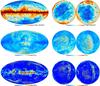 |
Fig. 1 DL fitted parameter maps. The top row corresponds to the dust mass surface density, ΣMd, the middle row to the starlight intensity heating the bulk of the dust, Umin, and the bottom row to the fraction of dust luminosity emitted by dust heated with high stellar intensities, fPDR. The left column corresponds to a Mollweide projection of the sky in Galactic coordinates, and the centre and right columns correspond to orthographic projections of the southern and northern hemispheres centred on the corresponding Galactic poles. A Galactic coordinate grid is plotted in the maps of the first row. Lines of ecliptic latitude at ± 10° are plotted in the maps of the bottom row. |
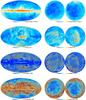 |
Fig. 2 DL derived parameters. The top row corresponds to the dust luminosity surface density, ΣLd, the second row shows the mean intensity heating the dust, ⟨ U ⟩, the third row shows the χ2 per degree of freedom of the fit, χ2/ N.d.o.f., and the bottom row the S/N map of the dust mass surface density ΣMd. |
Figure 2 shows a map of the dust emitted luminosity surface density, ΣLd, the mean intensity heating the dust, ⟨ U ⟩, the χ2 per degree of freedom (d.o.f.) of the fit, χ2/ N.d.o.f., and a map of the S/N ratio of the dust mass surface density ΣMd.
The χ2/ N.d.o.f. map scatter around unity in the high Galactic latitude areas, where the data uncertainties are noise-dominated. The χ2/ N.d.o.f. is slightly larger than 1 in the inner Galactic disk and several other localized areas. In the outer Galactic disk the χ2/ N.d.o.f. is smaller than 1, presumably due to overestimation of the uncertainties. Over much of the sky, the fit to the FIR SED is not as good as in Pl-MBB; the MBB fit has three fitting parameters in contrast with the DL model which has only two, ΣMd and Umin9.
4.2. Dust model photometric performance: residual maps
As shown in the χ2/ N.d.o.f. map in Fig. 2, the DL model fits the observed SED satisfactorily (within 1σ) over most of the sky areas. However, the model SEDs have systematic departures from the observed SED in the inner Galactic disk, at low ecliptic latitude, and in localized regions. We note that the spectral index of the dust FIR−submm opacity is fixed in the DL model; it cannot be adjusted to match the observed SED closely. This is why MBB spectra (with one extra effective degree of freedom) fits the observed SED better in some regions. The departures of the model in the low ecliptic latitude regions could be caused by defects in the zodiacal light estimation (and removal) from the photometric maps that the model cannot accommodate. In the Magellanic Clouds (MC) the DL model fails to fit the data10. The MC exhibit surprisingly strong emission at submm and millimetre wavelengths. Planck Collaboration XVII (2011) conclude that conventional dust models cannot account for the observed 600−3000 μm emission without invoking unphysically large amounts of very cold dust. Draine & Hensley (2012) suggest that magnetic dipole emission from magnetic grain materials could account for the unusually strong submm emission from the Small MC.
Figures 3 and 4 show the model departures from the photometric constraints used in the fits. Each panel shows the difference between the model predicted intensity and the observed intensity, divided by the observed uncertainty. The systematic departures show that the physical model being used does not have sufficient parameters or flexibility to fit the data perfectly.
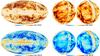 |
Fig. 3 Comparison between the model and the IRAS data used to constrain the fit. Each panel shows the model departure from the data defined as Dep. = (Model − Map)/Uncertainty. The top row corresponds to IRAS 60, and the bottom row to IRAS 100. The polar projection maps are smoothed to 1° resolution to highlight the systematic departures, and lines of Ecliptic latitude at ± 10° are added for reference. |
By increasing γ (i.e. the PDR component), the DL model can increase the IRAS 60 to IRAS 100 ratio to high values, without contributing much to the Planck intensities. Thus, in principle, the model should never underpredict the IRAS 60 emission. Figure 3 shows the model performance for fitting the IRAS bands; several high latitude areas (mostly with fPDR = 0) have IRAS 60 overpredicted and IRAS 100 underpredicted. Both model components (the diffuse cloud and PDR components) have an IRAS 60/IRAS 100 intensity ratio slightly larger than the ratio observed in these regions. There are several areas where the IRAS 60/IRAS 100 ratio is below the value for the best-fit Umin, hence in these areas the model (with fPDR = 0) overpredicts IRAS 60. This systematic effect is at the 1−2σ level (i.e. 10−20%).
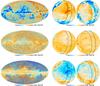 |
Fig. 4 Comparison between the model and the Planck data used to constrain the fit. Each panel shows the model departure from the data defined as Dep. = (Model−Map)/Uncertainty. The top row corresponds to Planck 857, the central row to Planck 545, and the bottom row to Planck 353. The polar projection maps are smoothed to 1° resolution to highlight the systematic departures, and lines of Ecliptic latitude at ± 10° are added for reference. |
In the inner Galactic disk the DL model tends to underpredict the 350 μm and overpredict the 850 μm emission (see Fig. 4). The observed SED is systematically steeper than the DL SED in the 350−850 μm range (i.e. between Planck 857 and Planck 353). Similar results were found in the central kiloparsec of M31 in the 250−500 μm range (DA14). The MBB fit of these regions, presented in Pl-MBB, finds larger values of the opacity spectral index β (β ≈ 2.2) than the typical value found in the low-and mid-range dust surface density areas (β ≈ 1.65). The DL SED peak can be broadened by increasing the PDR component (i.e. by raising γ or fPDR), but it cannot be made steeper than the γ = 0 (fPDR = 0) models, and the model therefore fails to fit the 350−850 μm SED in these regions.
Following DA14, we define  (6)as the effective power-law index of the DL dust opacity between 350 μm and 850 μm, where κDL ∗ F is the assumed absorption cross-section per unit dust mass convolved with the respective Planck filter. For the DL model11 this ratio is ΥDL ≈ 1.8.
If the dust temperatures in the fitted DL model were left unchanged, then the predicted Planck 857/Planck 353 intensity ratio could be brought into agreement with observations if ΥDL were changed by δΥ given by  (7)where we denote Iν(Planck...) the observed Planck intensity, and Iν(DL ...) the corresponding intensity for the DL model.
Figure 5 shows the δΥ map, i.e. the correction to the spectral index of the submm dust opacity that would bring the DL SED into agreement with the observed SED if the dust temperature distribution is left unchanged. The observed SED is steeper than the DL model in the inner Galactic disk (δΥDL ≈ 0.3) and shallower in the MC (δΥDL ≈ −0.3). The correction to the spectral index δΥ is positive on average. The average value of δΥ tends to increase with ΣMd, but the scatter of the individual pixels is always larger than the mean. The large dispersion in the low surface brightness areas is mainly due to CIB anisotropies. The dispersion in bright sky areas, e.g. along the Galactic plane and in molecular clouds off the plane, may be an indicator of dust evolution, i.e. variations in the FIR emission properties of the dust grains in the diffuse ISM.
Modifying the spectral index of the dust opacity in the model would change Umin and thereby the dust mass surface density. The δΥ map should be regarded as a guide on how to modify the dust opacity in future dust models, rather than as the exact correction to be applied to the opacity law per se.
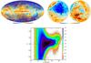 |
Fig. 5 Correction to the FIR opacity power law-index (δΥ) needed to bring the DL SED into agreement with the Planck observations. The polar projection maps are smoothed to 1° resolution to highlight the systematic departures. The bottom row shows the scatter of the δΥ map as a function of ΣMd. Colour corresponds to the logarithm of the density of points, i.e. the logarithm of number of sky pixels that have a given (ΣMd,δΥ) value in the plot. The curves correspond to the mean value and the ±1σ dispersion. |
4.3. Robustness of the mass estimate
4.3.1. Importance of IRAS 60
To study the potential bias introduced by IRAS 60, due to residuals of zodiacal light estimation (whose relative contribution is the largest in the IRAS 60 band) or the inability of the DL model to reproduce the correct SED in this range, one can perform modelling without the IRAS 60 constraint. In this case we set γ = 0, i.e. we allow only the diffuse cloud component (fPDR = 0), and so we have a two-parameter model.
Figure 6 shows the ratio of the dust mass estimated without using the IRAS 60 constraint and with γ = 0 to that estimated using IRAS 60 and allowing γ to be fitted (i.e. our original modelling). The left panel shows all the sky pixels and the right panel only the pixels with fPDR> 0. In the mid-and-high-range surface mass density areas (ΣMd> 105M⊙ kpc-2), where the photometry has good S/N, both models agree well, with a rms scatter below 5%. The inclusion or exclusion of the IRAS 60 constraint does not significantly affect our dust mass estimates in these regions. In the low surface density areas, inclusion of the IRAS 60 does not change the ΣMd estimate in the fPDR> 0 areas, but it leads to an increase of the ΣMd estimate in the fPDR = 0 pixels. In the fPDR = 0 areas, the model can overpredict IRAS 60 in some pixels, and therefore, when this constraint is removed, the dust can be fitted with a larger Umin value reducing the ΣMd needed to reproduce the remaining photometric constraints. In the fPDR> 0 areas, the PDR component has a small contribution to the longer wavelengths constraints, and therefore removing the IRAS 60 constraint and PDR component has little effect in the ΣMd estimates.
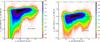 |
Fig. 6 Comparison between the dust mass estimates when the IRAS 60 constraint is excluded or included in the fit. The left panel shows all the sky pixels, and the right panel only the fPDR> 0 pixels. The vertical axis corresponds to the ratio of the inferred mass density of a fit without using the IRAS 60 constraint to that obtained when this constraint is present (see text). Colour corresponds to the logarithm of the density of points (see Fig. 5). The curve corresponds to the mean value. |
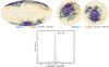 |
Fig. 7 Comparison between the dust mass estimates obtained with and without the DIRBE 140 and DIRBE 240 photometric constraints. The top row shows maps of the ratio between the two dust mass estimates, and the bottom row shows the corresponding histogram. Both model fits are performed using a 1° FWHM Gaussian PSF. The difference between the dust mass estimates is relatively small (within a few percent) and so it is safe to perform a modelling of the sky without the DIRBE constraints. In the bottom row, the points below 0.8 and over 1.2 were added to the 0.8 and 1.2 bars, respectively. |
4.3.2. Dependence of the mass estimate on the photometric constraints
The Planck and IRAS data do not provide photometric constraints in the 120 μm <λ< 300 μm range. This is a potentially problematic situation, since the dust SED typically peaks in this wavelength range. We can add the DIRBE 140 and DIRBE 240 constraints in a low resolution (FWHM> 42′) modelling to test this possibility.
We compare two analyses performed using a 1° FWHM Gaussian PSF. The first uses the same photometric constraints as the high resolution modelling (WISE, IRAS, and Planck), and the second additionally uses the DIRBE 140 and DIRBE 240 constraints. The results are shown in Fig. 7. Both model fits agree very well, with differences between the dust mass estimates of only a few percent. Therefore, our dust mass estimates are not substantially affected by the lack of photometric constraints near the SED peak. This is in agreement with similar tests carried out in Pl-MBB.
4.3.3. Validation on M31
In Appendix A we compare our dust mass estimates in the Andromeda galaxy (M31) with estimates based on an independent data set and processing pipelines. Both analyses use the DL model. This comparison allows us to analyse the impact of the photometric data used in the dust modelling. We conclude that the model results are not sensitive to the specific data sets used to constrain the FIR dust emission, validating the present modelling pipeline and methodology.
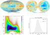 |
Fig. 8 Comparison between DL and MBB AV estimates, denotedAV,DL andAV,MBB respectively. The top row shows the ratio of theAV,MBB andAV,DL maps. The polar projection maps are smoothed to 1° resolution to highlight the systematic departures. The bottom row shows the ratio of theAV,MBB andAV,DL estimates as a function of theAV,DL estimate (left) and its histogram (right). In the bottom left panel the colour corresponds to the logarithm of the density of points (see Fig. 5). The curves correspond to the mean value and the ± 1σ dispersion. TheAV,DL andAV,MBB values used in this comparison are derived from a fit of the same data sets. |
5. Comparison between the DL and MBB optical exctinction estimates
We now compare the DL optical extinction estimates with those from the MBB dust modelling presented in Pl-MBB, denotedAV,DL andAV,MBB respectively. We perform a DL dust modeling of the same Planck data as in Pl-MBB (i.e. the nominal mission maps)12, the same IRAS 100 data, but our DL modelling also includes IRAS 60 and WISE 12 constraints. The DL model has two extra parameters (γ and qPAH) that can adjust the IRAS 60 and WISE 12 intensity fairly independently of the remaining bands. Therefore, the relevant data that both models are using in determining the FIR emission are essentially the same. The MBB extinction map has been calibrated with external (optical) observational data, and so this comparison allows us to test the DL modelling against those independent data.
Pl-MBB estimated the optical extinction13AV,QSO for a sample of QSOs from the SDSS survey. A single normalization factor Π was chosen to convert their optical depth τ353 map (the parameter of the MBB that scales linearly with the total dust emission, similar to the DL ΣMd) into an optical extinction map: AV,MBB ≡ Π τ353.
DL is a physical dust model and therefore fitting the observed FIR emission directly provides an optical extinction estimate, without the need for an extra calibration. However, if the DL dust model employs incorrect physical assumptions (e.g. the value of the FIR opacity), it may systematically over or under estimate the optical extinction corresponding to observed FIR emission.
Figure 8 shows the ratio of the DL and MBB AV estimates. The top row shows the ratio map. The bottom row shows its scatter and histogram. Over most of the sky (0.1 mag <AV,DL< 20 mag), the AV,DL values are larger than the AV,MBB by a factor of 2.40 ± 0.40. This discrepancy is roughly independent of AV,DL. The situation changes in the very dense areas (inner Galactic disk). In these areas (AV,DL ≈ 100 mag), the AV,DL are larger than the AV,MBB estimates by 1.95 ± 0.10.
In the diffuse areas (AV,DL ≲ 1), where the AV,MBB has been calibrated using the QSOs, AV,DL overestimates AV,MBB, and therefore AV,DL should overestimate AV,QSO by a similar factor. This mismatch arises from two factors. (1) The DL dust physical parameters were chosen so that the model reproduces the SED proposed by Finkbeiner et al. (1999), based on FIRAS observations. It was tailored to fit the high latitude Iν/N(H i) with Umin ≈ 1. The high latitude SED from Planck observations differs from that derived from FIRAS observations. The difference depends on the frequency and can be as high as 20% (Planck Collaboration VIII 2014). The best fit to the mean Planck + IRAS SED on the QSO lines of sight is obtained for Umin ≈ 0.66. The dust total emission (luminosity) computed for the Planck and for the Finkbeiner et al. (1999) SED are similar. The dust total emission per unit of optical reddening (or mass) scales linearly with Umin. Therefore, we need 1/0.66 ≈ 1.5 more dust mass to reproduce the observed luminosity. This is in agreement with the results of Planck Collaboration Int. XVII (2014) who have used the dust −H i correlation at high Galactic latitudes to measure the dust SED per unit of H i column density. They find that their SED is well fit by the DL model for Umin = 0.7 after scaling by a factor 1.45. (2) The optical extinction per gas column density used to construct the DL model is that of Bohlin et al. (1978). Recent observations show that this ratio needs to be decreased by a factor of approximately 1/1.4 (Liszt 2014a,b). Combining the two factors, we expect the AV,DL to overestimate the AV,QSO by about a factor of 2.
6. Renormalization of the model extinction map
We proceed in our analysis of the model results characterizing how the ratio between the optical extinction from the DL model and that measured from the optical photometry of QSOs depends on Umin. We introduce the sample of QSOs we use in Sect. 6.1, and compare the DL and QSO AV estimates in Sect. 6.2. Based on this analysis, we propose a renormalization of the optical extinction derived from the DL model (Sect. 6.3). The renormalized extinction map is compared to that derived by Schlafly et al. (2014, hereafterSGF) from stellar reddening using the Pan-STARRS1 (Kaiser et al. 2010) data.
6.1. The QSO sample
SDSS provides photometric observations for a sample of 272 366 QSOs, which allow us to measure the optical extinction for comparison with that from the DL model. A subsample of 105 783 (an earlier data release) was used in Pl-MBB to normalize the opacity maps derived from the MBB fits in order to produce an extinction map.
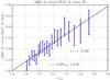 |
Fig. 9 Ratio between the QSO extinction estimates AV,QSO and the DL extinction estimates AV,DL, as a function of the fitted parameter Umin. The ratio is the slope ϵ obtained fitting AV,QSO versus AV,DL in each Umin bin (see text). It is approximated by a linear function of Umin. |
The use of QSOs as calibrators has several advantages over other cross-calibrations:
-
QSOs are extragalactic, and at high redshift, so all the detected dust in a given pixel is between the QSO and us, a major advantage with respect to maps generated from stellar reddening studies;
-
the QSO sample is large and well distributed across diffuse (AV ≲ 1) regions at high Galactic latitude, providing good statistics;
-
SDSS photometry is very accurate and well understood.
In Appendix B we describe the SDSS QSO catalogue in detail, and how for each QSO we measure the extinction AV,QSO from the optical SDSS observations.
6.2. AV,QSO – AV,DL comparison
In this section, we present a comparison of the DL and QSO extinction, as a function of the fitted parameter Umin. The DL and QSO estimates of AV are compared in the following way. We sort the QSO lines of sight with respect of the Umin value and divide them in 20 groups having (approximately) equal number of QSOs each. For each group of QSOs, we measure the slope ϵ(Umin) fitting the AV,QSO versus AV,DL data with a line going through the origin. In Fig. 9, ϵ(Umin) is plotted versus the mean value of Umin for each group. We observe that ϵ(Umin), a weighted mean of AV,QSO/AV,DL in each Umin bin, depends on Umin. The slope obtained fitting the AV,QSO versus AV,DL for the whole sample of QSOs is ⟨ ϵ ⟩ ≈ 0.495. Therefore, on average the DL model overpredicts the observed AV,QSO by a factor of 1/0.495 = 2.0, with the discrepancy being larger for sightlines with smaller Umin values. There is a 20% difference between the 2.4 factor that arises from the comparison between AV,DL and AV,QSO indirectly via the MBB AV fit, and the mean factor of 2.0 found here. This is due to the use of a different QSO sample (Pl-MBB used a smaller QSO sample), which accounts for 10% of the difference, and to differences in the way the QSO AV is computed from the SDSS photometry, responsible of the remaining 10%.
For a given FIR SED, the DL model predicts the optical reddening unambiguously, with no freedom for any extra calibration. However, if one had the option to adjust the DL extinction estimates by multiplying them by a single factor (i.e. ignoring the dependence of ϵ on Umin), one would reduce the optical extinction estimates by a factor of 2.0.
6.3. Renormalization of the AV,DL map in the diffuse ISM
We use the results of the AV,QSO –AV,DL comparison (Sect. 6.2 and Fig. 9) to renormalize the AV,DL map in the diffuse ISM. The ratio between the two extinction values is well approximated as a linear function of Umin:  (8)Thus, we define a renormalized DL optical reddening as14:
  (9)Empirically, AV,RQ is our best estimator of the QSO extinction AV,QSO. Pl-MBB proposed the dust radiance (the total luminosity emitted by the dust) as a tracer of dust column density in the diffuse ISM. This would be expected if the radiation field heating the dust were uniform, and the variations of the dust temperature were only driven by variation of the dust FIR-submm opacity in the diffuse ISM. The dust radiance is proportional to Umin × AV,DL. Our best fit of the renormalization factor as a function of Umin is an intermediate solution between the radiance and the model column density (AV,DL). The scaling factor in Eq. (8) increases with Umin but with a slope smaller than 1. Figure 9 shows that our renormalization is a better fit of the data than the radiance.
6.4. Validation of the renormalized extinction with stellar observations
We compare the renormalized extinction AV,RQ to the extinction estimated by SGF from optical stellar observations, denoted AV,Sch. SGF presented a map of the dust reddening to 4.5 kpc derived from Pan-STARRS1 stellar photometry. Their map covers almost the entire sky north of declination −30° at a resolution of 7″−14″. In the present analysis, we discard the sky areas with | b | < 5° to avoid the Galactic disk where a fraction of the dust is farther than 4.5 kpc, and therefore, traced by dust in emission, but not present in the SGF absorption map.
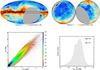 |
Fig. 10 Comparison between the renormalized DL AV estimates (AV,RQ), and those derived from optical stellar observations (AV,Sch). The top row shows the AV maps derived from optical stellar observations. The b = ± 5° lines have been added for reference. The bottom row left panel compares the renormalized AV,RQ estimates with those derived from optical stellar observations AV,Sch in the | b | > 5° sky. The agreement of these independent AV estimates is a successful test of our empirical renormalization. The bottom row right panel show the histogram of the difference of the two AV estimates, also in the | b | > 5° sky. |
Figure 10 shows the comparison between the renormalized DL AV estimates (AV,RQ) with the stellar observations based AV,Sch estimates in the | b | > 5° sky. The agreement between both AVestimates is remarkable. The difference between the estimates (AV,Sch−AV,RQ) has a mean of 0.02 mag and scatter (variance) of 0.12 mag. This comparison validates our renormalized DL AV estimates as a good tracer of the dust optical extinction in the | b | > 5° sky. Our optical extinction estimate (AV,RQ) was tailored to match the QSOs AV estimates. QSOs were observed in diffuse diffuse Galactic lines of sight (most of the QSOs have AV ≈ 0.1). The agreement of the AV,Sch and AV,RQ estimates extends the validity of the DL renormalized estimate (AV,RQ) to greater column densities. The scatter of AV,Sch–AV,RQ provides an estimate of the uncertainties in the different AV estimates.
7. FIR SEDs per unit of optical extinction
The DL model parameter Umin and the QSO data are used to compress the FIR IRAS and sub-mm Planck observations of the diffuse ISM to a set of 20 SEDs normalized per AV, which we present and discuss.
The parameter Umin is mainly determined by the wavelength where the SED peaks; as a corollary, SEDs for different values of Umin differ significantly. The AV values obtained from the QSO analysis,AV,QSO, allow us to normalize the observed SEDs (per unit of optical extinction) and generate a one-parameter family of Iν/AV. This family is indexed by the Umin parameter; the QSO lines of sight are grouped according to the fitted Galactic Umin value. We divide the sample of good QSOs in 20 bins, containing 11 212 QSOs each15.
To obtain the Iν/AV values we proceed as follows. For each band and Umin, we would like to perform a linear regression of the Iν values as a function ofAV,QSO. The large scatter and non-Gaussian distribution ofAV,QSO and the scatter on Iν make it challenging to determine such a slope robustly. Therefore, we smooth the maps to a Gaussian PSF with 30′ FWHM to reduce the scatter on Iν, redo the dust modelling (to obtain a coherent Umin estimate), and perform the regression on the smoothed (less noisy) maps. The non-Gaussian distribution ofAV,QSO do not introduce any bias in the slope found16.
Figure F11 presents the set of SEDs. The left panel shows the SEDs for the different Umin values. The right panel shows each SED divided by the mean to highlight the differences between the individual SEDs.
The complex statistics of theAV,QSO estimates, which depend on variations in QSO intrinsic spectra, makes it hard to obtain a reliable estimate of the uncertainties in the (normalizing) AV. However, the statistical uncertainties are not dominant because they average out thanks to the large size of the QSOs sample. The accuracy of our determination of the FIR intensities per unit of optical extinction is mainly limited by systematic uncertainties on the normalization by AV. Pl-MBB estimated the AV over a subsample of the QSOs, and their estimates differ from ours by ≈14%. When we compare ourAV,QSO estimates from those of SGF based on stellar photometry (Sect. 6.4), we find an agreement within 5−10% over the QSO lines of sight, Therefore, it is reasonable to assume ourAV,QSO estimates are uncertain at a 10% level. The instrumental calibration uncertainties (≲6% at Planck frequencies) translate directly to the FIR intensities per unit of optical extinction. Therefore, the normalization of each SED may be uncertain up to about ≈15%.
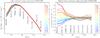 |
Fig. 11 FIR measured intensity per unit of optical extinction as a function of the fitted parameter Umin. In the right panel, the SEDs are divided by the mean SED, i.e. normalized with the SED per unit of optical extinction obtained without binning on Umin. |
In Fig. 12, the specific intensities per unit of optical extinction are compared with the DL model. The four panels correspond to the spectral bands: IRAS 100; Planck 857; Planck 545; and Planck 353. In each panel, the black curve corresponds to the DL intensity normalized by AV, and the red curves to the DL intensity normalized by AV,RQ, i.e. the model intensity scaled by the renormalization factor in Eq. (8). The DL model under-predicts the FIR intensities per unit of optical extinction AV by significant amounts, especially for sightlines with low fitted values of Umin, but the renormalization of the DL AV values brings into agreement the observed and model band intensities per unit of extinction. This result shows that the DL model has approximately the correct SED shape to fit the measured SEDs for the diffuse ISM, and that a Umin-dependent renormalization brings the DL model into agreement with the IRAS and Planck data. It is also a satisfactory check of the consistency of our data analysis and model fitting. Indeed, the SED values in Fig. 12 are derived from a linear fit between the data andAV,QSO, the renormalization factor from a linear fit betweenAV,QSO andAV,DL (see Fig. 9), andAV,DL from the DL model fit of the data (see Sect. 3.2).
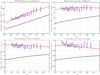 |
Fig. 12 Specific intensities per unit of optical extinction derived from a linear fit between the dust emission maps andAV,QSO are plotted with red crosses and error bars in blue versus the fitted parameter Umin. The top row corresponds to IRAS 100 (left) and Planck 857 (right) and the bottom row to Planck 545 (left) and Planck 353 (right). The DL model values are plotted in black and the renormalized model in red. This plot shows that a Umin-dependent renormalization brings the DL model into agreement with the IRAS and Planck data. |
8. Optical extinction and FIR emission in molecular clouds
We extend our assessment of the DL extinction maps to molecular clouds using extinction maps from 2MASS stellar colours that are presented in Sect. 8.1. In Sect. 8.2, we compare them with the original and renormalized estimates derived from the DL model. We discuss a model renormalization for molecular clouds in Sect. 8.3.
8.1. Extinction maps of molecular clouds
Schneider et al. (2011) presented optical extinction maps, denoted AV,2M, of several clouds computed using stellar observations from the 2MASS catalogue in the J, H, and K bands. We use the maps of the Cepheus, Chamaeleon, Ophiuchus, Orion, and Taurus cloud complexes. The Schneider et al. (2011) AV maps were computed using a 2′ Gaussian PSF, and we smooth them to a 5′ Gaussian PSF to perform our analysis. We corrected the 2MASS maps for a zero level offset that is fitted with an inclined plane with an algorithm similar to the one used to estimate the background in the analysis of the KINGFISH sample of galaxies in AD12. The algorithm iteratively and simultaneously matches the zero level across the AV,RQ and AV,2M maps and defines the areas that are considered background. The uncertainty on the zero level of the AV maps is smaller than 0.1 magnitude. It is significant only for the map areas with the lowest AV values.
Figure F13 shows the 2MASS AV,2M map, the DL Umin map, theAV,DL map (divided by 3.07, see Sect. 8.2 ) and the renormalized AV,RQ map for the Chamaeleon region. The inner (high AV) areas correspond to the lowest Umin values, as expected since the stellar radiation field heating dust grains is attenuated when penetrating into molecular clouds. The cloud complexes show a similar AV −Umin trend.
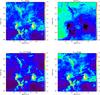 |
Fig. 13 2MASS and DL estimates in the Chamaeleon cloud region. The top row shows the (background corrected) 2MASS AV,2M map (left) and the DL Umin map (right). The bottom row shows the DLAV,DL estimate divided by 3.07 (left), and the renormalized model AV,RQ estimates (right). (See Sect. 8.2 for a derivation of the 3.07 factor) |
8.2. Comparison of 2MASS and DL extinction maps in molecular clouds
For each cloud, we find an approximate linear relation between the AV,2M and theAV,DL maps as illustrated for the Chamaeleon cloud in the left panel of Fig. 14. After multiplicative adjustment, theAV,DL and AV,2M estimates agree reasonably well. However, as in the diffuse ISM, the (FIR based)AV,DL estimates are significantly larger than the (optical) AV,2M estimates. For the selected clouds, the DL model overestimates the 2MASS stellar AV by factors of 2−3. Table 2 provides the multiplicative factors needed to make the 2MASS AV maps agree with the DL AV maps.
Mean ratio between the DL and 2MASS extinction estimates in molecular clouds.
We compare the renormalized AV,RQ versus AV,2M values in the right panel of Fig. 14 for the Chamaeleon cloud and in Fig. 15 for all of the clouds. We find that the model renormalization, computed to bring into agreement the DL and QSO AV estimates in the diffuse ISM, also accounts quite well (within 10%) for the discrepancies between 2MASS and DL AV estimates in molecular clouds in the 0 <AV< 3 range, and even does passably well (within 30%) up to AV ≈ 8.
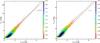 |
Fig. 14 2MASS and DL AV comparison in the Chamaeleon cloud. The left panel shows theAV,DL versus AV,2M values, and the right panel the renormalized AV,RQ versus AV,2M values. The diagonal lines correspond to y = 3.07x, and y = x respectively, and the curves correspond to the mean value. |
8.3. Renormalization ofAV,DL in molecular clouds.
In the diffuse ISM analysis, we concluded that Umin is tracing variations in the radiation field and the dust opacity. Both phenomena are also present in molecular clouds, but their relative contribution in determining the SED peak (and therefore Umin) need not be the same as in the diffuse ISM. Therefore, a renormalization of the DL AV based on 2MASS data may be different from that determined using the QSOs.
In Fig. 16 we compare the DL and 2MASS AV estimates for pixels from the five cloud complexes with 1 <AV,2M< 5. Similarly to Fig. 9, but using the 2MASS AV estimates instead of those from QSOs, we plot the ratioAV,DL/AV,2M as a function of the fitted Umin. For each Umin value, the solid curve corresponds to the best fit slope of theAV,DL versus AV,2M values (i.e. it is an estimate of a weighted mean of theAV,DL/AV,2Mratio). The straight solid line corresponds to a fit to the solid curve in the 0.2 <Umin< 1.0 range. In this fit, each Umin is given a weight proportional to the number of pixels that have this value in the clouds (i.e. most of the weight is for the pixels within the 0.2 <Umin< 0.8 range). The dashed line corresponds to the renormalization proposed in Sect. 6.3 (Eq. (9)) for the diffuse ISM.
The straight line in Fig. 16 corresponds to a renormalization tailored to bring into agreement theAV,DL and AV,2M estimates, i.e. a 2MASS renormalization for molecular clouds, denoted AV,RC. The 2MASS renormalization is given by  (10)Empirically, AV,RC is our best estimator of the 2MASS extinction AV,2M. It is satisfactory for the renormalization method to find that the 2MASS normalization factor for molecular clouds is quite close to the one for the diffuse ISM.
9. Discussion
In Sects. 9.1 and 9.2, we relate the difference between the DL model and AV estimates from QSO observations to dust emission properties and their evolution within the diffuse ISM. The renormalization method we propose to correct empirically for this discrepancy is discussed in Sect. 9.3.
9.1. DL FIR emission and optical extinction disagreement
In the diffuse ISM, the DL model provides good fits to the SED of Galactic dust from WISE, IRAS, and Planck data, as it has been the case in the past for external galaxies observed with Spitzer and Herschel. However, the fit is not fully satisfactory because the AV values from the model do not agree with those derived from optical colours of QSOs for the diffuse ISM and stars for molecular clouds. The optical extinction discrepancy can be decomposed in two levels: (1) the mean factor of 1.9 between the DL and QSOs AV values; and (2) the dependence of the ratio between the DL and QSO AV values on Umin.
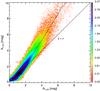 |
Fig. 15 Comparison of the renormalized AV,RQ and 2MASS AV,2M estimates. The individual pixels of the Cepheus, Chamaeleon, Ophiuchus, Orion, and Taurus clouds are combined. Colour corresponds to the logarithm of the density of points (see Fig. 5). The diagonal line corresponds to y = x, and the curve to the mean value. |
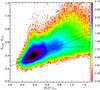 |
Fig. 16 Renormalization of the DL AV values in molecular clouds. Pixels from the five molecular complexes with 1 <AV,2M< 5 are included here. Colours encode the logarithm of the density of points (see Fig. 5). For each Umin value, the solid curve corresponds to the best fit slope of theAV,DL versus AV,2M values. The straight solid line corresponds to a fit to the solid curve in the 0.2 <Umin< 1.0 range, where each Umin is given a weight proportional to the number of pixels that have this value in the clouds. The straight solid line provides the AV,RC renormalization, and the dashed line that derived from the QSO analysis. |
The result of the SED fit depends on the spectral shape of the dust opacity. A spectral difference makes the DL model fit with a lower Umin value than the true radiation field intensity, which turns into an increase of the AV estimates17. The mean factor between the DL and QSOs AV values could also be indicating that the DL dust material has a FIR–submm opacity per unit of optical extinction that is too low.
The dependency of the ratio between the DL and QSO AV values on Umin shows that variations in the value of the FIR−submm dust opacity per unit of optical extinction, or its spectral shape, are needed across the sky; we take this to be evidence of dust evolution. This discrepancy will be present for all dust models based on fixed dust optical properties, possibly with a different magnitude depending of the details of the specific model.
Fanciullo et al. (2015) have used three dust models, the DL, Compiègne et al. (2011) and Jones et al. (2013) models, to fit the Planck SEDs in Table 3 and compare results. We note that the SEDs listed in the Table and used by Fanciullo et al. (2015) are the DL model results obtained fitting the same Planck and IRAS data as in Pl-MBB (see Sect. 2). This study, a follow-up of our data analysis, confirms our interpretation of our DL modelling in two ways. First, the mean ratio between the model and QSO AV values is different for each model. The best match between model and data is obtained for the model of Jones et al. (2013), which uses a FIR–submm opacity per unit of optical extinction18 larger than that of the DL model. Second, the three models fail in the same way to reproduce the variations in the emission per unit extinction with a variable ISRF intensity.
Fanciullo et al. (2015) also present fits of the Planck SEDs in Table 3 with a MBB spectrum (see their Appendix A). The dust FIR-submm opacity per unit extinction and the temperature obtained from these empirical fits display the same anti-correlation as that observed for the dust models between AV and the ISRF intensity. Thus, the dust models and MBB fits provide the same evidence for changes in the FIR-submm dust opacity in the diffuse ISM. Fanciullo et al. (2015) estimate that the amplitude of the variations must be ~20% to account for the typical (± 1σ around the mean) variations of the dust SEDs, and 40−50% for the full range.
FIR SEDs per unit of optical extinction.
9.2. Dust evolution in the diffuse ISM
We relate the Planck evidence for variations of the FIR–submm dust opacity to earlier studies of dust evolution in the ISM.
The extinction curve is known to vary through the ISM (Cardelli et al. 1989; Fitzpatrick & Massa 2007), especially in the UV but also in the near-IR (Fitzpatrick & Massa 2009). Similarly, the mid-IR dust emission presents variations of colour ratios between bands (Miville-Deschênes et al. 2002; Flagey et al. 2009). It is one of the successes of models like DL07 to be able accommodate this kind of evolution by adapting the size distribution of each component (Weingartner & Draine 2001), as well as the radiation field intensity for emission.
With the observations of FIR dust emission by the ISOPHOT camera onboard ISO and the PRONAOS balloon, it was however demonstrated that adapting the size distribution could not explain the low grain temperatures observed in dense filaments (Del Burgo et al. 2003; Stepnik et al. 2003). These papers argue that the intrinsic dust opacity in the FIR increases by a factor of a few, and that this can be achieved by modifying the grain structure and composition itself. Indeed, dust is known to be more emissive as composite aggregates than as compact grains (Stognienko et al. 1995; Köhler et al. 2011). The number of observations has since increased and confirmed this tendency (Del Burgo & Laureijs 2005; Ridderstad et al. 2006; Planck Collaboration XXV 2011), but primarily in the dense ISM (AV larger than a few magnitudes). More recently with Spitzer and Planck observations such variations in the dust FIR opacity have been identified in the diffuse ISM, with amplitudes comparable to those observed before in the dense medium (Bot et al. 2009; Martin et al. 2012; Planck Collaboration XI 2014; Planck Collaboration Int. XVII 2014).
It is reasonable to accommodate the increase of dust opacity in the dense ISM by invoking coagulation (Köhler et al. 2011; Ysard et al. 2012, 2013). However, dust models face now a new challenge. Since the timescale for dust coagulation increases for decreasing density, this solution does not hold in the diffuse, low-density, ISM. Variations in grain mantles composition and thickness through the accretion of carbon and cumulative irradiation have been proposed by Jones et al. (2013) and Ysard et al. (2015) as a main dust evolutionary process within the diffuse ISM. Differences in the past history of dust grains, i.e. in their evolutionary cycle between the diffuse ISM and molecular clouds, could also contribute to the observed scatter in the shape, size and composition of dust grains in the diffuse ISM (Martin et al. 2012). Modelling is needed to test whether these ideas can match the signature of dust evolution reported in this paper.
9.3. Optical exctinction AV estimates of dust models
To obtain an accurate AV map of the sky, we proposed two renormalizations of the AV estimates derived from the DL model (AV,RQ in Eq. (9) and AV,RC in Eq. (10)) that compensates for the discrepancy between the observed FIR emission and the optical extinction for the diffuse ISM and molecular clouds. Essentially, the renormalization rescales one of the model outputs (the dust optical extinction AV) by a function of Umin, to match data. Planck Collaboration Int. XXVIII (2015) presented an independent comparison of the renormalized AV,RQ estimates with γ-ray observations in the Chamaeleon cloud. They concluded that the renormalized AV,RQ estimates are in closer agreement with γ-ray AV estimates than the (non-renormalized)AV,DL estimates. We now discuss the model renormalization in a more general context.
The renormalized DL estimates (AV,RQ and AV,RC) provide a good AV determination in the areas where they were calibrated, but they do not provide any insight into the physical dust properties per se; the renormalized dust model becomes simply a family of SEDs used to fit the data, from which we construct and calibrate an observable quantity (AV,RQ and AV,RC). Unfortunately, the fitted parameters of the renormalized model (Umin) lack a physical interpretation: Umin is not solely tracing the heating intensity of the radiation field, as assumed in DL.
The AV estimate of the DL dust model is a function of its fitted parameters, i.e. AV = f(ΣMd,qPAH,γ,Umin). In general, if we fit a dust model with several parameters, AV will be a function of the most relevant parameters19. The DL model assumes AV = f(ΣMd) = k × ΣMd, with 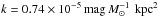 . Our proposed renormalizations are a first step towards a functional renormalization by extending AV = k × ΣMd into AV = g(Umin) × k × ΣMd, where we take g(Umin) to be a linear function of Umin. Due to the larger scatter in the QSO AV estimates, only a simple linear function g(Umin) can be robustly estimated in the diffuse ISM. In molecular clouds, where the data are less noisy, one could find a smooth function g′(Umin), which better matches theAV,DL/AV,2M fit for each Umin (i.e. in Fig. 16, the solid curve flattens for Umin> 0.8, departing from its linear fit).
Unfortunately any renormalization procedure, while leading to a more accurate AV estimate, does not provide any further insight into the dust physical properties. Real physical knowledge will arise from a new generation of dust models that should be able to predict the correct optical extinction AV from first principles. The next generation of dust models should be able to fit the empirical SEDs presented in Sect. 7 directly. While such a new generation of dust models is not yet available, we can for now correct for the systematic departures via Eqs. (9) and (10) for the diffuse ISM and molecular clouds, respectively.
10. Conclusions
We present a full-sky dust modelling of the new Planck data, combined with ancillary IRAS and WISE data, using the DL dust model. We test the model by comparing these maps with independent estimates of the dust optical extinction AV using SDSS QSO photometry and 2MASS stellar data. Our analysis provides new insight on interstellar dust and a new AV map over the full sky.
The DL model fits the observed Planck, IRAS, and WISE SEDs well over most of the sky. The modelling is robust against changes in the angular resolution, as well as adding DIRBE 140 and DIRBE 240 photometric constraints. The high resolution parameter maps that we generated trace the Galactic dusty structures well, using a state-of-the-art dust model.
In the diffuse ISM, the DL AV estimates are larger than estimates from QSO optical photometry by approximately a factor of 2, and this discrepancy depends systematically on Umin. In molecular clouds, the DL AV estimates are larger than estimates based on 2MASS stellar colours by a factor of about 3. Again, the discrepancy depends in a similar way on Umin.
We conclude that the current parameter Umin, associated with the peak wavelength of the SED, does not trace only variations in the intensity of the radiation field heating the dust; Umin also traces dust evolution: i.e. variations in the optical and FIR properties of the dust grains in the diffuse ISM. DL is a physical dust model. Physical dust models have the advantage that, if successful, they give some support to the physical assumptions made about the interstellar dust and ISM properties that they are based on. Unfortunately, the deficiency found in this study indicates that some of the physical assumptions of the model need to be revised.
We provide a one-parameter family of SEDs per unit of dust optical extinction in the diffuse ISM. These SEDs, which relate the dust emission and absorption properties, are independent of the dust/gas ratio or problems inferring total H column density from observations. The next generation of dust models will need to reproduce these new SED estimates.
We propose an empirical renormalization of the DL AV map as a function of the DL Umin parameter. The proposed renormalization (AV,RQ), derived to match the QSO AV estimates for the diffuse ISM, also brings into agreement the DL AV estimates with those derived from stellar colours for the | b | > 5 deg sky using the Pan-STARRS1 data (SGF), and towards nearby molecular clouds in the 0 <AV< 5 range using the 2MASS survey. We propose a second renormalized DL AV estimate (AV,RC) tailored to trace the AV estimates in molecular clouds more precisely.
The renormalized map AV,RQ based on our QSOs analysis is our most accurate estimate of the optical extinction in the diffuse ISM. Comparison of the AV,RQ map against other tracers of interstellar extinction that probe different environments, would further test its accuracy and check for any potential systematics. A comparison with Fermi data towards the Chamaeleon molecular cloud shows that the AV,RQ map more closely matches the γ-ray diffuse emission than the 353 GHz opacity and radiance maps from Pl-MBB, but not as well as the fit obtained combining H i, CO, and dark neutral medium maps, which indicates significant differences in the FIR-submm dust emission properties between these gas components, not taken into account in our renormalization (Planck Collaboration Int. XXVIII 2015).
Planck (http://www.esa.int/Planck) is a project of the European Space Agency (ESA) with instruments provided by two scientific consortia funded by ESA member states (in particular the lead countries France and Italy), with contributions from NASA (USA) and telescope reflectors provided by a collaboration between ESA and a scientific consortium led and funded by Denmark.
From now on we will refer to the WISE, IRAS, and DIRBE bands as WISE 12, IRAS 60, IRAS 100, DIRBE 100, DIRBE 140, and DIRBE 240, by attaching the band reference wavelength (in μm) to the spacecraft or instrument name, and to the Planck bands as Planck 857, Planck 545, Planck 353, Planck 217, Planck 143, and Planck 100, by attaching the band reference frequency (in GHz) to the spacecraft name.
The current CO maps are noisy in the low surface brightness areas, and therefore subtracting these small contributions increases the noise level significantly.
The zodiacal light emission contributes mainly at scales larger than 30′, therefore, its contribution is subtracted when we retain the large scales of the SDF map.
The new IRIS data reduction and a description are available at http://www.cita.utoronto.ca/~mamd/IRIS/IrisOverview.html
A full description of HEALPix and its software library can be found at http://healpix.jpl.nasa.gov
For the size distribution in the DL models, the mass fraction contributed by PAH particles containing NC< 106 C atoms is 1.478 qPAH.
In the details of their size distributions and dust composition (e.g. the lack of ices), these models will not be as appropriate for dust in dark molecular clouds.
The qPAH parameter does not affect significantly the FIR SED; it only affects significantly the WISE 12 photometry. The fPDR parameter affect mostly IRAC 60 photometry, without contributing significantly to the remaining FIR bands.
The MC appear as two red spots in the southern hemisphere in the top row of Fig. 4.
If the Planck filters were monochromatic at the nominal frequencies, then ΥDL = 1.82 (see Table 2 in DA14). For the real Planck filters the ΥDL value is a constant close to 1.8.
TheAV,DLestimates based on the full mission Planck maps (the maps used in the remaining sections of this paper), and the nominal mission Planck maps differ by only a few percent over most of the sky.
Pl-MBB actually determine optical reddening E(B − V) for the QSO sample. Since a fixed extinction curve with RV = 3.1 (see Appendix B.2) was used, this is equivalent to determining the optical extinction AV.
We add the letter Q to indicate the renormalization using theAV,QSO.
A few of the bins contain 11 213 QSOs.
See discussion in Appendix B.2, and Fig. B.2.
For example, if an MBB with T = 19 K, β = 1.9 is fitted with an MBB with β = 1.8, using the IRAS 100, Planck 857, Planck 545, and Planck 353 bands, then the fitted amplitude will be 30% larger than the original one. Therefore, a discrepancy of δΥ = 0.1 is likely to produce a bias in the AV estimates of the order of 30%.
The dust optical properties from this model are derived from recent laboratory data on silicates and amorphous carbons.
In the MBB approach, one should consider a function of the form AV = f(τ353,T,β).
Both dust mass surface density maps correspond to the line of sight projected densities, not corrected for the M31 inclination.
We will denote the QSO redshift as ζ, instead of the usual z to avoid confusion with the longest wavelength SDSS filter z.
See the discussion following Eq. (B.6).
Acknowledgments
The development of Planck has been supported by: ESA; CNES and CNRS/INSU-IN2P3-INP (France); ASI, CNR, and INAF (Italy); NASA and DoE (USA); STFC and UKSA (UK); CSIC, MICINN, JA, and RES (Spain); Tekes, AoF, and CSC (Finland); DLR and MPG (Germany); CSA (Canada); DTU Space (Denmark); SER/SSO (Switzerland); RCN (Norway); SFI (Ireland); FCT/MCTES (Portugal); and PRACE (EU). A description of the Planck Collaboration and a list of its members, including the technical or scientific activities in which they have been involved, can be found at http://www.sciops.esa.int/index.php?project=planck&page=Planck_Collaboration. The research leading to these results has received funding from the European Research Council under the European Union’s Seventh Framework Programme (FP7/2007−2013)/ERC grant agreement No. 267934.
References
- Abazajian, K. N., Adelman-McCarthy, J. K., Agüeros, M. A., et al. 2009, ApJS, 182, 543 [NASA ADS] [CrossRef] [Google Scholar]
- Aniano, G., Draine, B. T., Calzetti, D., et al. 2012, ApJ, 756, 46 [Google Scholar]
- Boggess, N. W., Mather, J. C., Weiss, R., et al. 1992, ApJ, 397, 420 [NASA ADS] [CrossRef] [Google Scholar]
- Bohlin, R. C., Savage, B. D., & Drake, J. F. 1978, ApJ, 224, 132 [NASA ADS] [CrossRef] [Google Scholar]
- Boselli, A., Eales, S., Cortese, L., et al. 2010, PASP, 122, 261 [NASA ADS] [CrossRef] [Google Scholar]
- Bot, C., Helou, G., Boulanger, F., et al. 2009, ApJ, 695, 469 [NASA ADS] [CrossRef] [Google Scholar]
- Cardelli, J. A., Clayton, G. C., & Mathis, J. S. 1989, ApJ, 345, 245 [NASA ADS] [CrossRef] [Google Scholar]
- Ciesla, L., Boquien, M., Boselli, A., et al. 2014, A&A, 565, A128 [Google Scholar]
- Compiègne, M., Verstraete, L., Jones, A., et al. 2011, A&A, 525, A103 [NASA ADS] [CrossRef] [EDP Sciences] [Google Scholar]
- de Vaucouleurs, G., de Vaucouleurs, A., Corwin, Jr., H. G., et al. 1991, Third Reference Catalogue of Bright Galaxies (New York: Springer) [Google Scholar]
- Del Burgo, C., & Laureijs, R. J. 2005, MNRAS, 360, 901 [NASA ADS] [CrossRef] [Google Scholar]
- Del Burgo, C., Laureijs, R. J., Ábrahám, P., & Kiss, C. 2003, MNRAS, 346, 403 [NASA ADS] [CrossRef] [Google Scholar]
- Desert, F.-X., Boulanger, F., & Puget, J. L. 1990, A&A, 237, 215 [NASA ADS] [Google Scholar]
- Doi, Y., Takita, S., Ootsubo, T., et al. 2015, PASJ, 67, 50 [NASA ADS] [Google Scholar]
- Draine, B. T., & Hensley, B. 2012, ApJ, 757, 103 [CrossRef] [Google Scholar]
- Draine, B. T., & Lee, H. M. 1984, ApJ, 285, 89 [Google Scholar]
- Draine, B. T., & Li, A. 2007, ApJ, 657, 810 [NASA ADS] [CrossRef] [Google Scholar]
- Draine, B. T., Dale, D. A., Bendo, G., et al. 2007, ApJ, 663, 866 [NASA ADS] [CrossRef] [Google Scholar]
- Draine, B. T., Aniano, G., Krause, O., et al. 2014, ApJ, 780, 172 [NASA ADS] [CrossRef] [Google Scholar]
- Dwek, E. 1998, ApJ, 501, 643 [NASA ADS] [CrossRef] [Google Scholar]
- Fanciullo, L., Guillet, V., Aniano, G., et al. 2015, A&A, 580, A136 [NASA ADS] [CrossRef] [EDP Sciences] [Google Scholar]
- Fazio, G. G., Hora, J. L., Allen, L. E., et al. 2004, ApJS, 154, 10 [NASA ADS] [CrossRef] [Google Scholar]
- Finkbeiner, D. P., Davis, M., & Schlegel, D. J. 1999, ApJ, 524, 867 [NASA ADS] [CrossRef] [Google Scholar]
- Fitzpatrick, E. L. 1999, PASP, 111, 63 [NASA ADS] [CrossRef] [Google Scholar]
- Fitzpatrick, E. L., & Massa, D. 2007, ApJ, 663, 320 [NASA ADS] [CrossRef] [EDP Sciences] [Google Scholar]
- Fitzpatrick, E. L., & Massa, D. 2009, ApJ, 699, 1209 [NASA ADS] [CrossRef] [Google Scholar]
- Flagey, N., Noriega-Crespo, A., Boulanger, F., et al. 2009, ApJ, 701, 1450 [NASA ADS] [CrossRef] [Google Scholar]
- Górski, K. M., Hivon, E., Banday, A. J., et al. 2005, ApJ, 622, 759 [NASA ADS] [CrossRef] [Google Scholar]
- Griffin, M. J., Abergel, A., Abreu, A., et al. 2010, A&A, 518, L3 [Google Scholar]
- Jones, A. P., Fanciullo, L., Köhler, M., et al. 2013, A&A, 558, A62 [NASA ADS] [CrossRef] [EDP Sciences] [Google Scholar]
- Kaiser, N., Burgett, W., Chambers, K., et al. 2010, in SPIE Conf. Ser., 7733 [Google Scholar]
- Kawada, M., Baba, H., Barthel, P. D., et al. 2007, PASJ, 59, 389 [Google Scholar]
- Kennicutt, R. C., Armus, L., Bendo, G., et al. 2003, PASP, 115, 928 [NASA ADS] [CrossRef] [Google Scholar]
- Kennicutt, R. C., Calzetti, D., Aniano, G., et al. 2011, PASP, 123, 1347 [NASA ADS] [CrossRef] [Google Scholar]
- Köhler, M., Guillet, V., & Jones, A. 2011, A&A, 528, A96 [NASA ADS] [CrossRef] [EDP Sciences] [Google Scholar]
- Li, A., & Draine, B. T. 2001, ApJ, 554, 778 [Google Scholar]
- Liszt, H. 2014a, ApJ, 783, 17 [NASA ADS] [CrossRef] [Google Scholar]
- Liszt, H. 2014b, ApJ, 780, 10 [NASA ADS] [CrossRef] [Google Scholar]
- Martin, P. G., Roy, A., Bontemps, S., et al. 2012, ApJ, 751, 28 [NASA ADS] [CrossRef] [Google Scholar]
- Mathis, J. S., Mezger, P. G., & Panagia, N. 1983, A&A, 128, 212 [NASA ADS] [Google Scholar]
- Meisner, A. M., & Finkbeiner, D. P. 2014, ApJ, 781, 5 [NASA ADS] [CrossRef] [Google Scholar]
- Miville-Deschênes, M.-A., & Lagache, G. 2005, ApJS, 157, 302 [NASA ADS] [CrossRef] [Google Scholar]
- Miville-Deschênes, M.-A., Boulanger, F., Joncas, G., & Falgarone, E. 2002, A&A, 381, 209 [NASA ADS] [CrossRef] [EDP Sciences] [Google Scholar]
- Murakami, H., Baba, H., Barthel, P., et al. 2007, PASJ, 59, 369 [Google Scholar]
- Neugebauer, G., Habing, H. J., van Duinen, R., et al. 1984, ApJ, 278, L1 [Google Scholar]
- Pâris, I., Petitjean, P., Aubourg, É., et al. 2014, A&A, 563, A54 [NASA ADS] [CrossRef] [EDP Sciences] [Google Scholar]
- Pilbratt, G. L., Riedinger, J. R., Passvogel, T., et al. 2010, A&A, 518, L1 [CrossRef] [EDP Sciences] [Google Scholar]
- Planck Collaboration XVII. 2011, A&A, 536, A17 [NASA ADS] [CrossRef] [EDP Sciences] [Google Scholar]
- Planck Collaboration XXIV. 2011, A&A, 536, A24 [Google Scholar]
- Planck Collaboration XXV. 2011, A&A, 536, A25 [NASA ADS] [CrossRef] [EDP Sciences] [Google Scholar]
- Planck Collaboration I. 2014, A&A, 571, A1 [NASA ADS] [CrossRef] [EDP Sciences] [Google Scholar]
- Planck Collaboration VIII. 2014, A&A, 571, A8 [NASA ADS] [CrossRef] [EDP Sciences] [Google Scholar]
- Planck Collaboration XI. 2014, A&A, 571, A11 [NASA ADS] [CrossRef] [EDP Sciences] [Google Scholar]
- Planck Collaboration XIV. 2014, A&A, 571, A14 [NASA ADS] [CrossRef] [EDP Sciences] [Google Scholar]
- Planck Collaboration Int. XVII. 2014, A&A, 566, A55 [NASA ADS] [CrossRef] [EDP Sciences] [Google Scholar]
- Planck Collaboration I. 2015, A&A, submitted [arXiv:1502.01582] [Google Scholar]
- Planck Collaboration VIII. 2015, A&A, submitted [arXiv:1502.01587] [Google Scholar]
- Planck Collaboration IX. 2015, A&A, submitted [arXiv:1502.05956] [Google Scholar]
- Planck Collaboration Int. XXV. 2015, A&A, 582, A28 [NASA ADS] [CrossRef] [EDP Sciences] [Google Scholar]
- Planck Collaboration Int. XXVIII. 2015, A&A, 582, A31 [NASA ADS] [CrossRef] [EDP Sciences] [Google Scholar]
- Poglitsch, A., Waelkens, C., Geis, N., et al. 2010, A&A, 518, L2 [NASA ADS] [CrossRef] [EDP Sciences] [Google Scholar]
- Ridderstad, M., Juvela, M., Lehtinen, K., Lemke, D., & Liljeström, T. 2006, A&A, 451, 961 [NASA ADS] [CrossRef] [EDP Sciences] [Google Scholar]
- Rieke, G. H., Young, E. T., Engelbracht, C. W., et al. 2004, ApJS, 154, 25 [NASA ADS] [CrossRef] [Google Scholar]
- Schlafly, E. F., Green, G., Finkbeiner, D. P., et al. 2014, ApJ, 789, 15 [NASA ADS] [CrossRef] [Google Scholar]
- Schlegel, D. J., Finkbeiner, D. P., & Davis, M. 1998, ApJ, 500, 525 [NASA ADS] [CrossRef] [Google Scholar]
- Schneider, N., Bontemps, S., Simon, R., et al. 2011, A&A, 529, A1 [NASA ADS] [CrossRef] [EDP Sciences] [Google Scholar]
- Siebenmorgen, R., Voshchinnikov, N. V., & Bagnulo, S. 2014, A&A, 561, A82 [NASA ADS] [CrossRef] [EDP Sciences] [Google Scholar]
- Silverberg, R. F., Hauser, M. G., Boggess, N. W., et al. 1993, SPIE, 2019, 180 [Google Scholar]
- Skrutskie, M. F., Cutri, R. M., Stiening, R., et al. 2006, AJ, 131, 1163 [NASA ADS] [CrossRef] [Google Scholar]
- Stepnik, B., Abergel, A., Bernard, J.-P., et al. 2003, A&A, 398, 551 [NASA ADS] [CrossRef] [EDP Sciences] [Google Scholar]
- Stognienko, R., Henning, T., & Ossenkopf, V. 1995, A&A, 296, 797 [NASA ADS] [Google Scholar]
- Van den Berk, D. E., Richards, G. T., Bauer, A., et al. 2001, AJ, 122, 549 [NASA ADS] [CrossRef] [Google Scholar]
- Vilardell, F., Ribas, I., Jordi, C., Fitzpatrick, E. L., & Guinan, E. F. 2010, A&A, 509, A70 [NASA ADS] [CrossRef] [EDP Sciences] [Google Scholar]
- Weingartner, J. C., & Draine, B. T. 2001, ApJ, 548, 296 [NASA ADS] [CrossRef] [Google Scholar]
- Werner, M. W., Roellig, T. L., Low, F. J., et al. 2004, ApJS, 154, 1 [Google Scholar]
- Wright, E. L., Eisenhardt, P. R. M., Mainzer, A. K., et al. 2010, AJ, 140, 1868 [NASA ADS] [CrossRef] [Google Scholar]
- York, D. G., Adelman, J., John, E., Anderson, J. E. Jr., et al. 2000, ApJ, 120, 1579 [Google Scholar]
- Ysard, N., Juvela, M., Demyk, K., et al. 2012, A&A, 542, A21 [NASA ADS] [CrossRef] [EDP Sciences] [Google Scholar]
- Ysard, N., Abergel, A., Ristorcelli, I., et al. 2013, A&A, 559, A133 [NASA ADS] [CrossRef] [EDP Sciences] [Google Scholar]
- Ysard, N., Köhler, M., Jones, A., et al. 2015, A&A, 577, A110 [NASA ADS] [CrossRef] [EDP Sciences] [Google Scholar]
- Zubko, V., Dwek, E., & Arendt, R. G. 2004, ApJS, 152, 211 [NASA ADS] [CrossRef] [Google Scholar]
Appendix A: Comparison with Spitzer + Herschel modelling of the Andromeda galaxy
The Andromeda galaxy is the nearest large spiral galaxy. It provides a useful benchmark to validate the current dust modelling. Its isophotal radius is R25 = 95′ (de Vaucouleurs et al. 1991), corresponding to R25 = 20.6 kpc at the assumed distance d = 744 kpc (Vilardell et al. 2010).
Several authors have modelled the dust properties of M31. Planck Collaboration Int. XXV (2015) presented an independent study to M31 using Planck maps and MBB dust model. In particular DA14 presented a DL based modelling of M31 using the IRAC (Fazio et al. 2004) and MIPS (Rieke et al. 2004) instruments on Spitzer, and the PACS (Poglitsch et al. 2010) and SPIRE (Griffin et al. 2010) instruments on Herschel. This data set has 13 photometric constraints (IRAC 3.6 μm, 4.5 μm, 5.8 μm, and 8.0 μm, MIPS 24 μm, 70 μm, and 160 μm, PACS 70 μm, 100 μm, and 160 μm, and SPIRE 250 μm, 350 μm, and 500 μm) from a different set of instruments than those used in our analysis. The high resolution modelling traces the structures of M31 in great detail, providing maps of Umin and dust surface density, and enables a comparison to be made with gas and metallicity observations. The modelling techniques are described and validated on NGC 628 and NGC 6946 in AD12, and later expanded to the full KINGFISH galaxy sample in AD15.
We compare the dust mass surface density maps20 of the modelling presented by DA14 (from now on called “Herschel”) degraded to a 5′ Gaussian PSF, with the current modelling, called “Planck”. In the Herschel modelling, a tilted plane is fitted to the background areas, and subtracted from the original images to remove the Milky Way cirrus emission. Therefore, we need to add the cirrus emission back to the Herschel mass estimates before comparing to the Planck modelling. The zero level of the Herschel modelling was restored with an algorithm similar to that used to estimate the background planes in the KINGFISH dust modelling (see AD12). This algorithm iteratively fits an inclined plane to the difference in mass surface densities over the background points.
M31 does not have considerable quantities of cold dust, which would be detected in the Planck modelling but not in the Herschel modelling. Therefore, we expect both modellings to agree well.
Figure A.1 presents the comparison of the two dust models. The Herschel and Planck approaches agree very well: the resolved mass differences between the two analyses is small, only 10 % across most of the galaxy. The remaining parameter estimates also agree well. In conclusion, the model results appear not to be sensitive to the specific data sets used to constrain the FIR dust emission. This comparison validates the present modelling pipeline and methodology.
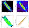 |
Fig. A.1 Comparison of M31 maps as seen by Herschel and Planck. The top row shows maps of the dust mass generated using Spitzer and Herschel data at high resolution (left) and the current estimates using IRAS and Planck data (right). The bottom row shows the ratio map of the two mass estimates (convolved to a common resolution and with the zero level matched) on the left, and their scatter on the right. The diagonal lines in the bottom right panel correspond to a one-to-one relationship and a ± 20% difference about that. The colour in the last panel corresponds to the density of points. Even though the two analyses are based on completely independent data, they agree remarkably well, differing by less than 10% across most of the galaxy. |
Appendix B: QSO Av estimation
The intrinsic colours of an unobscured QSO depend strongly on its redshift21 (ζ). We first estimate the (redshift dependent) unobscured QSO colour for each band pair. By comparing each QSO colours with the expected unobscured colours, we can estimate its reddening. Assuming a typical dust extinction curve, we can combine the reddening estimates of the band pairs into a single extinction estimate for each QSO. This analysis relies on the fact that the mean colour excess of a group of QSO scales linearly with the DL AV estimates (see Fig. B.2).
Appendix B.1: SDSS QSO catalogue
The SDSS is a photometric and spectroscopic survey, using a dedicated 2.5-m telescope at Apache Point Observatory in New Mexico. It has produced high quality observations of approximately 104 deg2 of the northern sky in five optical and near-IR bands: u, g, r, i, and z, centred at 354.3 nm, 477.0 nm, 623.1 nm, 762.5 nm, and 913.4 nm respectively (York et al. 2000). The SDSS seventh data release (DR7, Abazajian et al. 2009) contains a sample of 105 783 spectroscopically confirmed QSOs, and the SDSS tenth data release (DR10, Pâris et al. 2014) contains an additional sample of 166 583 QSOs.
In order to avoid absorption from the intergalactic medium, each SDSS band is only usable up to the redshift at which the Lyα line (121.57 nm vacuum wavelength) enters (from the blue side) into the filter. Therefore, we can use the u-band, for QSOs with ζ< 1.64, g-band for ζ< 2.31, r-band for ζ< 3.55, i-band for ζ< 4.62, and z-band for ζ< 5.69. We also limit the study to 0.35 <ζ< 3.35, to have enough QSOs per unit of redshift to estimate reliably the redshift-dependent unobscured QSO intrinsic colour (see Section B.2). We also remove the few QSOs that lie in a line of sight where the Galactic dust is very hot (Umin> 1.05), very cold (Umin< 0.4), very luminous (Ldust> 108L⊙ kpc-2), or where there is strong extinction (AV> 1). This leaves 261 841 useful QSOs.
Appendix B.2: Unobscured QSO intrinsic colours and extinction estimation
A typical QSO spectrum has several emission and absorption lines superimposed on a power-law-like continuum. Depending on the QSO redshift, the lines fall in different filters. Therefore, for each optical band pair (X,Y), the unobscured QSO intrinsic colour CX,Y(ζ) depends on the QSO redshift. Given two photometric bands X and Y, in order to estimate the unobscured QSO intrinsic colour CX,Y(ζ), we proceed as follows.
We will see that the intrinsic dust properties appear to depend on the parameter Umin. Therefore, to avoid introducing a potential bias when computing CX,Y(ζ), we group the lines of sight according to Umin, and analyse each group independently. The functions CX,Y(ζ) should, in principle, not depend on Umin, and therefore, all the estimates CX,Y(ζ,Umin) should be similar for the different Umin sets. Working independently on each Umin, for each redshift ζ we choose all the QSOs in the interval [ ζ − 0.05,ζ + 0.05 ], or the 2000 closest QSOs if there are more than 2000 QSOs in the interval, and fit the QSOs colour (X − Y) as a function of the dust column density:  (B.1)whereAV,DL is the DL estimated dust extinction in each QSO line of sight. The function CX,Y(ζ,Umin) is the best estimate of the colour difference (X − Y) of an unobscured QSO (AV,DL = 0) at redshift ζ, estimated from the lines of sight of dust fitted with Umin. The function ηX,Y(ζ,Umin) should be essentially independent of ζ22. Variations in the function ηX,Y(ζ,Umin) with respect to Umin give us information about the dust properties.
Once we compute CX,Y(ζ,Umin) for the different values of Umin, we average them for each redshift ζ to obtain CX,Y(ζ). For each Umin and ζ, the weight given to each CX,Y(ζ,Umin) value is proportional to the number of QSO in the [ ζ − 0.05,ζ + 0.05 ] interval. Figure B.1 shows the results of this unobscured QSO intrinsic colour estimation algorithm for the bands i and z. The functions Ci,z(ζ,Umin) are shown for the different values of Umin, using redder lines for larger Umin, and greener for smaller Umin. Their weighted mean Ci,z(ζ) is shown in black.
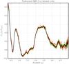 |
Fig. B.1 Unobscured QSO intrinsic colours, as a function of redshift (ζ), for the bands i and z. The functions Ci,z(ζ,Umin), are shown for the different values of Umin, using redder traces for larger Umin, and greener for smaller Umin. Their weighted mean Ci,z(ζ) is shown in black. The Lyα line affects the i band photometry for ζ> 4.62, but we restrict our analysis to ζ< 3.35 to have enough QSOs per redshift interval. For ζ> 3.35 the estimated Ci,z(ζ) becomes noisy. |
For each QSO, we define its reddening EX,Y as: 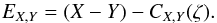 (B.2)The EX,Y values should not depend on the redshift, and therefore we can group all the QSOs of a given Umin into a sub sample with the same intrinsic colour. We note that no additional hypotheses on the QSO spectral shape or dust extinction curve need to be made to compute the QSO intrinsic colours. Working with all the QSOs with a given Umin, we fit
 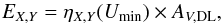 (B.3)and identify the outlier QSOs that depart by more than 3σ from the expected linear relationship. Figure B.2 shows the typical QSO Eg,r versusAV,DL fit for Umin = 0.6. In this case, ηg,r(Umin = 0.6) = 0.19. Although the QSO EX,Y versusAV,DL relationship has large scatter due to variations in the QSOs spectra (continuum and lines) and intrinsic obscuration in the QSOs, as long as there is no selection bias with respect toAV,DL our study should be robust. The fact that the mean QSO EX,Y for eachAV,DL (curve) and the best fit of the QSO EX,Y versusAV,DL (straight line) in Fig. B.2 agree remarkably well, supports the validity of the preceding analysis.
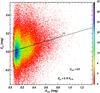 |
Fig. B.2 Colour excess Eg,r versusAV,DL for the QSOs with Umin = 0.6. Colour corresponds to the density of points (see Fig. 5). The straight line corresponds to the best fit for all the QSOs. For eachAV,DL, the black curve corresponds to the mean Eg,r for the QSOs in an interval with a half-width δAV,DL = 0.01. Even though the QSOs show significant scatter, the Eg,r versusAV,DL relationship is very linear; the mean Eg,r for eachAV,DL curve does not show significant departures from the straight line. |
Once we have computed EX,Y for all the band pairs and Umin, we remove the QSOs that are considered as outliers in any of the computations to obtain a cleaner sample of good QSOs. We reiterate the full procedure twice using the good QSO sample form the previous iteration, resulting in a final cleanest sample containing 224 245 QSOs with ζ< 3.35 (for which we have Lyα free photometry in the r-, i-, and z-bands), 135,953 with ζ< 2.31 (where we can use the r-band), and 77 633 QSO with ζ< 1.64, where we can use all the SDSS bands. We have an estimate of the intrinsic colours CX,Y, and an estimate of the reddening EX,Y for each QSO that is retained by the redshift constraints.
Even though the unobscured QSO intrinsic colours are computed independently for each band pair, we do obtain consistent results across the band pairs, i.e.  (B.4)holds for all the bands X, Y, and Z, over all the redshifts ζ considered. Working with the H i column density maps as an estimate of the extinction instead of theAV,DL gives very similar estimates of CX − Y(ζ), and is independent of any dust modelling, so this means we did not translate potential dust modelling systematics into our QSO estimates.
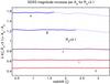 |
Fig. B.3 QSO magnitude increase per unit of dust extinction AV as a function of the QSO redshift. We use an extinction curve with RV = 3.1. The u and g band curves are shown in a thinner trace for ζ> 1.64 and ζ> 2.31, the redshifts at which the intergalactic Lyα line can affect the photometry in these bands. |
In order to compare theAV,DL estimate with a QSO estimate, we need to derive a QSO extinction AV from the different colour excess EX,Y. We proceed as follows.
For a given QSO spectrum and extinction curve shape, we can compute the SDSS magnitude increase per dust extinction AX/AV for X = u,g,r,i, and z. These ratios depend on the assumed extinction curve and QSO spectral shape, and therefore on the QSO redshift. Using the QSO composite spectrum of Vanden Berk et al. (2001) and the extinction curve presented by Fitzpatrick (1999) parametrized via RV, we compute the ratios AX/AV:  (B.5)Figure B.3 shows δX(ζ,RV = 3.1) as a function of the QSO redshift ζ, for the different bands X = u,g,r,i, and z. Even though the QSO intrinsic colours are strong functions of its redshift, the extinction curves are smooth enough that δX(ζ,RV = 3.1) is mostly redshift independent.
Using the extinction curves with RV = 3.1 (which was also used to constrain the optical properties of the grains used in the DL model), for each redshift ζ, we define: ![Mathematical equation: \appendix \setcounter{section}{2} \begin{equation} \delta_{[X,Y]} (\zeta)= {1 \over \delta\,X(\zeta,R_V=3.1) \,-\, \delta\,Y(\zeta,R_V=3.1)}, \label{eq_eta} \end{equation}](/articles/aa/full_html/2016/02/aa24945-14/aa24945-14-eq270.png) (B.6)and
(B.6)and ![Mathematical equation: \appendix \setcounter{section}{2} \begin{equation} A_{V,{\rm QSO},[X,Y]} = \delta_{[X,Y]} \times E_{X,Y}. \label{eq_del} \end{equation}](/articles/aa/full_html/2016/02/aa24945-14/aa24945-14-eq271.png) (B.7)Finally, for each QSO, we define itsAV,QSO as the average of the AV,QSO, [ X,Y ] values for all the band pairs that are allowed by its redshift ζ.
(B.7)Finally, for each QSO, we define itsAV,QSO as the average of the AV,QSO, [ X,Y ] values for all the band pairs that are allowed by its redshift ζ.
Appendix C: Impact of the CIB anisotropies and instrumental noise on the parameter estimation
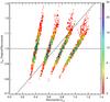 |
Fig. C.1 Comparison of the original and recovered dust mass under CIBA and instrumental noise simulation in the diffuse ISM for a 30′ resolution. Colour corresponds to the density of points (see Fig. 5). |
We study the impact of CIB anisotropies (CIBA) and instrumental (stochastic) noise in our mass estimates in the diffuse ISM (where their effect should be the largest). We simulate data by adding CIBA and instrumental noise to DL SEDs, and fit them with the same technique as we use to fit the observed data. The results quantify the deviations of the recovered parameters from the original ones.
We start by a family of four DL SEDs with Umin = 0.4, 0.6, 0.8, and 1.0, a typical fPDR = 0.05, and qPAH = 0.03. We normalize each SED to the mean AV found for the QSO lines of sight in each Umin. We replicate each SED 100 000 times, add CIB anisotropies and instrumental noise. The noise added has 2 components. We add (band-to-band) independent noise to simulate stochastic instrumental noise with amplitudes given by Pl-MBB, Table B.1, 30′ resolution. We further add a typical CIB SED (also from Pl-MBB, Table B.1, 30′ row), that is completely correlated across the Planck bands, and partially correlated with the IRAS bands, as recommended in Pl-MBB, Appendix B. We finally fit each simulated SED with DL model, as we did in the main data fit.
Figure C.1 shows the recovered ΣMd divided by the original ΣMd, and recovered Umin for the SEDs. Each set of points correspond to the different original Umin. The inclined solid line corresponds to the renormalization curve given by Eq. (9), (rescaled to match the mean AV of the simulated SEDs). There is not a global bias in the recovered ΣMd, nor Umin; the distribution of the recovered ΣMd and Umin are centered in the original values. Although CIBA and instrumental noise do generate a trend in the same direction as the renormalization, their impact is significantly smaller than the observed renormalization: they do not span the full range found over the QSOs lines of sight. Moreover, the renormalization found in Sect. 6.3 is independent of the modelling resolution; one obtain similar renormalization coefficients working at 5′, 30′, and 60′ FWHM. For those resolutions, the instrumental noise and CIBA have a very different magnitude, and therefore, their impact would be quite different. Therefore, CIBA and instrumental noise are not a significant source of the AV systematic departures with respect to Umin found in Sect. 6.3.
Appendix D: Maps in the Planck Legacy Archive
The maps of the dust model parameters, the dust extinction and the model predicted fluxes described in this paper can be obtained from the Planck Legacy Archive (PLA23). The maps are all at 5′(FWHM) angular resolution in the HEALPix representation with Nside = 2048.
For each quantity, but the χ2 of the fit per degree of freedom, there are 2 maps corresponding to the value presented and the corresponding uncertainty. Available maps include our best estimate of the dust extinction (the renormalized AV,RQ) expressed in magnitude units, and the best fit DL parameters: the dust mass surface density ΣMd expressed in M⊙ kpc-2 units, the starlight intensity heating the bulk of the dust, Umin in units of the ISRF estimated by Mathis et al. (1983) for the solar neighbourhood, the fraction of the dust luminosity from dust heated by intense radiation fields, fPDR in Eq. (2), which is a dimensionless number between 0 and 1, and the dust mass fraction in small PAH grains qPAH. We also provide the DL model predicted fluxes in the Planck, IRAS 60 and 100, and WISE 12 bands. Additional information about the file names and the data format is available in the Planck explanatory supplement24.
All Tables
All Figures
|
Fig. 1 DL fitted parameter maps. The top row corresponds to the dust mass surface density, ΣMd, the middle row to the starlight intensity heating the bulk of the dust, Umin, and the bottom row to the fraction of dust luminosity emitted by dust heated with high stellar intensities, fPDR. The left column corresponds to a Mollweide projection of the sky in Galactic coordinates, and the centre and right columns correspond to orthographic projections of the southern and northern hemispheres centred on the corresponding Galactic poles. A Galactic coordinate grid is plotted in the maps of the first row. Lines of ecliptic latitude at ± 10° are plotted in the maps of the bottom row. |
| In the text | |
|
Fig. 2 DL derived parameters. The top row corresponds to the dust luminosity surface density, ΣLd, the second row shows the mean intensity heating the dust, ⟨ U ⟩, the third row shows the χ2 per degree of freedom of the fit, χ2/ N.d.o.f., and the bottom row the S/N map of the dust mass surface density ΣMd. |
| In the text | |
|
Fig. 3 Comparison between the model and the IRAS data used to constrain the fit. Each panel shows the model departure from the data defined as Dep. = (Model − Map)/Uncertainty. The top row corresponds to IRAS 60, and the bottom row to IRAS 100. The polar projection maps are smoothed to 1° resolution to highlight the systematic departures, and lines of Ecliptic latitude at ± 10° are added for reference. |
| In the text | |
|
Fig. 4 Comparison between the model and the Planck data used to constrain the fit. Each panel shows the model departure from the data defined as Dep. = (Model−Map)/Uncertainty. The top row corresponds to Planck 857, the central row to Planck 545, and the bottom row to Planck 353. The polar projection maps are smoothed to 1° resolution to highlight the systematic departures, and lines of Ecliptic latitude at ± 10° are added for reference. |
| In the text | |
|
Fig. 5 Correction to the FIR opacity power law-index (δΥ) needed to bring the DL SED into agreement with the Planck observations. The polar projection maps are smoothed to 1° resolution to highlight the systematic departures. The bottom row shows the scatter of the δΥ map as a function of ΣMd. Colour corresponds to the logarithm of the density of points, i.e. the logarithm of number of sky pixels that have a given (ΣMd,δΥ) value in the plot. The curves correspond to the mean value and the ±1σ dispersion. |
| In the text | |
|
Fig. 6 Comparison between the dust mass estimates when the IRAS 60 constraint is excluded or included in the fit. The left panel shows all the sky pixels, and the right panel only the fPDR> 0 pixels. The vertical axis corresponds to the ratio of the inferred mass density of a fit without using the IRAS 60 constraint to that obtained when this constraint is present (see text). Colour corresponds to the logarithm of the density of points (see Fig. 5). The curve corresponds to the mean value. |
| In the text | |
|
Fig. 7 Comparison between the dust mass estimates obtained with and without the DIRBE 140 and DIRBE 240 photometric constraints. The top row shows maps of the ratio between the two dust mass estimates, and the bottom row shows the corresponding histogram. Both model fits are performed using a 1° FWHM Gaussian PSF. The difference between the dust mass estimates is relatively small (within a few percent) and so it is safe to perform a modelling of the sky without the DIRBE constraints. In the bottom row, the points below 0.8 and over 1.2 were added to the 0.8 and 1.2 bars, respectively. |
| In the text | |
|
Fig. 8 Comparison between DL and MBB AV estimates, denotedAV,DL andAV,MBB respectively. The top row shows the ratio of theAV,MBB andAV,DL maps. The polar projection maps are smoothed to 1° resolution to highlight the systematic departures. The bottom row shows the ratio of theAV,MBB andAV,DL estimates as a function of theAV,DL estimate (left) and its histogram (right). In the bottom left panel the colour corresponds to the logarithm of the density of points (see Fig. 5). The curves correspond to the mean value and the ± 1σ dispersion. TheAV,DL andAV,MBB values used in this comparison are derived from a fit of the same data sets. |
| In the text | |
|
Fig. 9 Ratio between the QSO extinction estimates AV,QSO and the DL extinction estimates AV,DL, as a function of the fitted parameter Umin. The ratio is the slope ϵ obtained fitting AV,QSO versus AV,DL in each Umin bin (see text). It is approximated by a linear function of Umin. |
| In the text | |
|
Fig. 10 Comparison between the renormalized DL AV estimates (AV,RQ), and those derived from optical stellar observations (AV,Sch). The top row shows the AV maps derived from optical stellar observations. The b = ± 5° lines have been added for reference. The bottom row left panel compares the renormalized AV,RQ estimates with those derived from optical stellar observations AV,Sch in the | b | > 5° sky. The agreement of these independent AV estimates is a successful test of our empirical renormalization. The bottom row right panel show the histogram of the difference of the two AV estimates, also in the | b | > 5° sky. |
| In the text | |
|
Fig. 11 FIR measured intensity per unit of optical extinction as a function of the fitted parameter Umin. In the right panel, the SEDs are divided by the mean SED, i.e. normalized with the SED per unit of optical extinction obtained without binning on Umin. |
| In the text | |
|
Fig. 12 Specific intensities per unit of optical extinction derived from a linear fit between the dust emission maps andAV,QSO are plotted with red crosses and error bars in blue versus the fitted parameter Umin. The top row corresponds to IRAS 100 (left) and Planck 857 (right) and the bottom row to Planck 545 (left) and Planck 353 (right). The DL model values are plotted in black and the renormalized model in red. This plot shows that a Umin-dependent renormalization brings the DL model into agreement with the IRAS and Planck data. |
| In the text | |
|
Fig. 13 2MASS and DL estimates in the Chamaeleon cloud region. The top row shows the (background corrected) 2MASS AV,2M map (left) and the DL Umin map (right). The bottom row shows the DLAV,DL estimate divided by 3.07 (left), and the renormalized model AV,RQ estimates (right). (See Sect. 8.2 for a derivation of the 3.07 factor) |
| In the text | |
|
Fig. 14 2MASS and DL AV comparison in the Chamaeleon cloud. The left panel shows theAV,DL versus AV,2M values, and the right panel the renormalized AV,RQ versus AV,2M values. The diagonal lines correspond to y = 3.07x, and y = x respectively, and the curves correspond to the mean value. |
| In the text | |
|
Fig. 15 Comparison of the renormalized AV,RQ and 2MASS AV,2M estimates. The individual pixels of the Cepheus, Chamaeleon, Ophiuchus, Orion, and Taurus clouds are combined. Colour corresponds to the logarithm of the density of points (see Fig. 5). The diagonal line corresponds to y = x, and the curve to the mean value. |
| In the text | |
|
Fig. 16 Renormalization of the DL AV values in molecular clouds. Pixels from the five molecular complexes with 1 <AV,2M< 5 are included here. Colours encode the logarithm of the density of points (see Fig. 5). For each Umin value, the solid curve corresponds to the best fit slope of theAV,DL versus AV,2M values. The straight solid line corresponds to a fit to the solid curve in the 0.2 <Umin< 1.0 range, where each Umin is given a weight proportional to the number of pixels that have this value in the clouds. The straight solid line provides the AV,RC renormalization, and the dashed line that derived from the QSO analysis. |
| In the text | |
|
Fig. A.1 Comparison of M31 maps as seen by Herschel and Planck. The top row shows maps of the dust mass generated using Spitzer and Herschel data at high resolution (left) and the current estimates using IRAS and Planck data (right). The bottom row shows the ratio map of the two mass estimates (convolved to a common resolution and with the zero level matched) on the left, and their scatter on the right. The diagonal lines in the bottom right panel correspond to a one-to-one relationship and a ± 20% difference about that. The colour in the last panel corresponds to the density of points. Even though the two analyses are based on completely independent data, they agree remarkably well, differing by less than 10% across most of the galaxy. |
| In the text | |
|
Fig. B.1 Unobscured QSO intrinsic colours, as a function of redshift (ζ), for the bands i and z. The functions Ci,z(ζ,Umin), are shown for the different values of Umin, using redder traces for larger Umin, and greener for smaller Umin. Their weighted mean Ci,z(ζ) is shown in black. The Lyα line affects the i band photometry for ζ> 4.62, but we restrict our analysis to ζ< 3.35 to have enough QSOs per redshift interval. For ζ> 3.35 the estimated Ci,z(ζ) becomes noisy. |
| In the text | |
|
Fig. B.2 Colour excess Eg,r versusAV,DL for the QSOs with Umin = 0.6. Colour corresponds to the density of points (see Fig. 5). The straight line corresponds to the best fit for all the QSOs. For eachAV,DL, the black curve corresponds to the mean Eg,r for the QSOs in an interval with a half-width δAV,DL = 0.01. Even though the QSOs show significant scatter, the Eg,r versusAV,DL relationship is very linear; the mean Eg,r for eachAV,DL curve does not show significant departures from the straight line. |
| In the text | |
|
Fig. B.3 QSO magnitude increase per unit of dust extinction AV as a function of the QSO redshift. We use an extinction curve with RV = 3.1. The u and g band curves are shown in a thinner trace for ζ> 1.64 and ζ> 2.31, the redshifts at which the intergalactic Lyα line can affect the photometry in these bands. |
| In the text | |
|
Fig. C.1 Comparison of the original and recovered dust mass under CIBA and instrumental noise simulation in the diffuse ISM for a 30′ resolution. Colour corresponds to the density of points (see Fig. 5). |
| In the text | |
Current usage metrics show cumulative count of Article Views (full-text article views including HTML views, PDF and ePub downloads, according to the available data) and Abstracts Views on Vision4Press platform.
Data correspond to usage on the plateform after 2015. The current usage metrics is available 48-96 hours after online publication and is updated daily on week days.
Initial download of the metrics may take a while.