| Issue |
A&A
Volume 536, December 2011
|
|
|---|---|---|
| Article Number | A88 | |
| Number of page(s) | 32 | |
| Section | Extragalactic astronomy | |
| DOI | https://doi.org/10.1051/0004-6361/201117952 | |
| Published online | 16 December 2011 | |
Non-standard grain properties, dark gas reservoir, and extended submillimeter excess, probed by Herschel in the Large Magellanic Cloud⋆
1
AIM, CEA/Saclay, L’Orme des Merisiers, 91191
Gif-sur-Yvette,
France
e-mail: This email address is being protected from spambots. You need JavaScript enabled to view it.
2
Centre d’Étude Spatiale des Rayonnements, CNRS,
9 Av. du Colonel
Roche, BP 4346,
31028
Toulouse,
France
3
Observatoire Astronomique de Strasbourg,
11 rue de
l’université, 67000
Strasbourg,
France
4
Space Telescope Science Institute, 3700 San Martin Drive, Baltimore, MD
21218,
USA
5
Institute of Astronomy, University of Cambridge,
Madingley Road,
Cambridge
CB3 0HA,
UK
6
314 Physics Building, Department of Physics and Astronomy,
University of Missouri, Columbia, MO
65211,
USA
7
Steward Observatory, University of Arizona,
933 North Cherry
Ave., Tucson,
AZ
85721,
USA
8
Spitzer Science
Center, California Institute of Technology, MS 220-6, Pasadena, CA
91125,
USA
Received:
25
August
2011
Accepted:
5
October
2011
Abstract
Context.Herschel provides crucial constraints on the IR SEDs of galaxies, allowing unprecedented accuracy on the dust mass estimates. However, these estimates rely on non-linear models and poorly-known optical properties.
Aims. In this paper, we perform detailed modelling of the Spitzer and Herschel observations of the LMC, in order to: (i) systematically study the uncertainties and biases affecting dust mass estimates; and to (ii) explore the peculiar ISM properties of the LMC.
Methods. To achieve these goals, we have modelled the spatially resolved SEDs with two alternate grain compositions, to study the impact of different submillimetre opacities on the dust mass. We have rigorously propagated the observational errors (noise and calibration) through the entire fitting process, in order to derive consistent parameter uncertainties.
Results. First, we show that using the integrated SED leads to underestimating the dust mass by ≃50% compared to the value obtained with sufficient spatial resolution, for the region we studied. This might be the case, in general, for unresolved galaxies. Second, we show that Milky Way type grains produce higher gas-to-dust mass ratios than what seems possible according to the element abundances in the LMC. A spatial analysis shows that this dilemma is the result of an exceptional property: the grains of the LMC have on average a larger intrinsic submm opacity (emissivity index β ≃ 1.7 and opacity κabs(160 μm) = 1.6 m2 kg-1) than those of the Galaxy. By studying the spatial distribution of the gas-to-dust mass ratio, we are able to constrain the fraction of unseen gas mass between ≃10, and ≃100% and show that it is not sufficient to explain the gas-to-dust mass ratio obtained with Milky Way type grains. Finally, we confirm the detection of a 500 μm extended emission excess with an average relative amplitude of ≃15%, varying up to 40%. This excess anticorrelates well with the dust mass surface density. Although we do not know the origin of this excess, we show that it is unlikely the result of very cold dust, or CMB fluctuations.
Key words: ISM: abundances / dust, extinction / galaxies: ISM / galaxies: dwarf / Magellanic Clouds / galaxies: starburst
Appendices are available in elctronic form at http://www.aanda.org
© ESO, 2011
1. Introduction
The infrared (IR) spectral energy distribution (SED) is widely used to derive the global properties of a system, such as its instantaneous star formation rate, its dust and eventually gas masses, and the compactness of the star forming region. The advent of the Herschel Space Observatory has opened the most important spectral window to perfect these diagnostics, by observing the far-IR to submillimeter (submm) wavelengths (60–600 μm). Indeed, this regime samples the peak and Rayleigh-Jeans wing of the dust emission. It consequently constrains the emission by grains in thermal equilibrium with the radiation field, present in the different phases of the interstellar medium (ISM), including the coldest, most massive components (down to dust temperatures of Tdust ≳ 12 K). This spectral domain is therefore crucial to derive accurate dust masses, and physical conditions, and can be used as a powerful, unprecedented tool to probe interstellar matter in regions where no other counterpart is accessible.
Unfortunately, there are several fundamental systematic unknowns inherent to dust modelling, which are questioning the reliability of these diagnostics. First, the microscopic properties of the grains are still poorly known. In the Milky Way, the most complete and accurate models are constrained by observations of high latitude cirrus clouds: their IR emission, ultraviolet (UV)-to-near-IR extinction, and elemental depletions (Zubko et al. 2004; Draine & Li 2007; Compiègne et al. 2011). The authors performing these models derive the size distribution and abundance of the different grain species – silicates, carbon grains (graphite or amorphous carbons) and polycyclic aromatic hydrocarbons (PAH). Zubko et al. (2004) demonstrated an important degeneracy by presenting complete fits of the same data set (Galactic emission, extinction and depletion), with five different dust compositions, alternating bare and coated grains, as well as crystalline and amorphous solids. Thus, the derived dust properties depend on the assumed chemical composition of each species. The UV to millimetre (mm) opacities are sensitive to the grain composition. They are derived from sparse constraints including astrophysical features, laboratory spectra of analogs of interstellar dust materials, and theoretical solid state physics (e.g. Weingartner & Draine 2001; Draine 2003b). Their universality is doubtful.
The second major source of uncertainties concerns the macroscopic variations of these microscopic grain properties, as a function of the environment. These variations are numerous; some are speculative:(i) PAHs are known to be destroyed in H ii regions (e.g. Madden et al. 2006); (ii) the variations in the RV parameter of the extinction curve is interpreted as variations of the grain size distribution (Draine 2003a; Fitzpatrick & Massa 2005); (iii) coagulation occurs in dense regions (e.g. Stepnik et al. 2003; Berné et al. 2007); (iv) blast waves are responsible for grain fragmentation and erosion in the low-velocity phase (Jones et al. 1996) and destruction close to the remnant (Reach et al. 2002); (v) the dust abundances and properties are thought to evolve with the metallicity of the ISM (Galliano et al. 2003, 2005, 2008a); (vi) a transition from amorphous to crystalline silicates is observed in protostellar objects (e.g. Hallenbeck et al. 2000; Poteet et al. 2011). This list is not exhaustive. Moreover, when considering the SED of a given region, it is possible to confuse variations of the physical properties of the grains (e.g. their optical properties) with variations of their physical conditions (e.g. the starlight intensity to which they are exposed). This problem becomes even more intricate, when considering the integrated SED of a galaxy.
The various processes controlling the lifecycle of dust throughout the ISM are not known with enough precision to break these kinds of degeneracies. Even the origin of interstellar dust is uncertain. The contribution of supernovae (SN) and asymptotic giant branch (AGB) stars to the observed content of ISM dust, and the dust growth in interstellar cloud is still debated (e.g. Galliano et al. 2008a; Draine 2009). Dust is believed to constantly evolve throughout the ISM, being photoprocessed, altered by cosmic rays, accreting atoms in dense regions, and being shattered in shocks (Jones 2004, for a review). We are compelled to find observational cases where there will be enough redundancy in the data to isolate one of these processes. This is the goal of this paper.
The present article scrutinizes the different methodological biases, as well as the fundamental physical processes affecting the dust mass estimate in galaxies. Our demonstration is performed on the Herschel and Spitzer observations of the Large Magellanic Cloud (LMC; d = 50 ± 2.5 kpc; Schaefer 2008). Due to its proximity, it is an ideal laboratory to study the variations of the far-IR properties, down to spatial scales of ≃10 pc (SPIRE500 μm angular resolution of 36′′). Moreover, it offers an environment containing massive star clusters, allowing us to study the impact of intense star formation on the surrounding ISM. Finally, its metallicity is moderately sub-solar, with (O/H)LMC ≃ 0.5 × (O/H)⊙ and (C/H)LMC ≃ 0.3 × (C/H)⊙ (Pagel 2003). The comparison of its dust properties with those of the Galaxy therefore provides insights on cosmic dust evolution.
In general, low-metallicity dwarf galaxies, a category to which the LMC belongs, have peculiar dust properties. They exhibit a deficit of PAH strength, that appears to be correlated with the metallicity of their ISM. The origin of this trend is still debated: (i) PAHs could be more massively destroyed by permeating hard radiation, in sub-solar ISM (e.g. Madden et al. 2006); (ii) the delayed injection of PAHs by AGB stars could explain their lower intrinsic abundance, in young systems (Galliano et al. 2008a); (iii) the PAHs could form in molecular clouds, which have a lower filling factor, in low-metallicity environments (e.g. Sandstrom et al. 2010).
The IR SED of dwarf galaxies usually peaks at shorter wavelengths, indicating hotter equilibrium grains, on average. In addition, the mid-IR continuum is steeply rising, similarly to what is observed in Galactic compact H ii regions (e.g. Peeters et al. 2002). This peculiar mid-IR continuum, was modelled by Galliano et al. (2003, 2005) with an increase of the very small grain abundances, which could be the consequence of the high number density of shock waves. It is consistent with the peculiar shape of the extinction curve, in the Magellanic clouds: their lower 2175 Å bump, and their steeper near-UV rise could be the result of an excess of small grains (Weingartner & Draine 2001; Galliano et al. 2003, 2005). This typical continumm shape was reported as a “mid-IR excess” compared to the Galactic SED by Bernard et al. (2008), in the LMC.
The dust-to-gas mass ratio increases with metallicity (Lisenfeld & Ferrara 1998; Draine et al. 2007; Galliano et al. 2008a; Engelbracht et al. 2008). At first order, it can be understood since dust is made out of the metals synthesized by the various stellar populations. However, the detailed dependency of the dust-to-gas mass ratio with the metallicity remains unknown. In addition, the gas mass, especially the molecular phase, is uncertain, because the CO-to-H2 conversion factor is a strong unknown function of the environment – in particular, it is a function of the metallicity. A given CO line intensity will translate in a larger molecular gas mass in a lower metallicity environments (e.g. Madden et al. 1997; Israel 1997; Leroy et al. 2007, 2009, 2011). Moreover, we can expect the presence of large quantities of H2 in regions where no CO at all is detected (Madden 2000). Bernard et al. (2008) unveiled a “far-IR excess”, compared to the gas column density, in the LMC, which is likely the evidence of such a gas reservoir.
Finally, at submm wavelengths, the SED of dwarf galaxies differs significantly from solar metallicity systems. Galliano et al. (2003, 2005) reported in four blue compact dwarf galaxies an excess emission at 850 μm (SCUBA) and 1.2 mm (MAMBO). Such an excess was then confirmed in other similar systems (Dumke et al. 2004; Galametz et al. 2009, 2010; Bot et al. 2010; Grossi et al. 2010). It extends up to centimetre (cm) wavelengths in the LMC and SMC (Israel et al. 2010; Planck Collaboration et al. 2011a). Although, the COBE data of our Galaxy presented a submm excess (Reach et al. 1995), the intensity of this excess is much more pronounced in low-metallicity systems. Several explanations are in competition, for the origin of this excess: (i) very cold dust, in dense clumps, accounting for a large fraction of the dust budget of the galaxy (Galliano et al. 2003, 2005; Galametz et al. 2009; O’Halloran et al. 2010); (ii) temperature dependent submm emissivity (Meny et al. 2007); (iii) rapidly spinning grains in addition to another component (Bot et al. 2010; Planck Collaboration et al. 2011a).
The first Herschel observations of the LMC showed that the slope of the submm SED was flatter than in the Galaxy (Gordon et al. 2010). Meixner et al. (2010) showed that modelling this SED with standard Galactic grain properties required too much mass, and therefore concluded that it required modified grain optical properties. Roman-Duval et al. (2010) confirmed the Bernard et al. (2008) “far-IR excess” toward several molecular clouds. Hony et al. (2010) demonstrated the complex structure of two massive starforming regions. Gordon et al. (2010) reported a SPIRE500 μm excess, which is likely the rise of the submm excess previously discussed.
The unprecedented sensitivity and wavelength coverage of Herschel, at far-IR/submm wavelengths, allow us, for the first time, to study in detail processes that were previously glimpsed at. With a rigorous method, accounting for the different sources of error, it is now possible to unveil the systematic effects inherent to SED modelling. The common assumptions, concerning the universality of dust properties, the accuracy of gas mass estimates, and the homogeneity of gas-to-dust mass ratios can be confronted by data. From a technical point of view, all the processes that have been previously described here define the required model parameters, as well as the unknowns when interpreting the IR/submm emission of the LMC.
For that purpose, the present paper is organized as follows. Section 2 presents the data set upon which we have based our analysis, and discusses the reference observational quantities we consider. In Sect. 3, we present our SED model, and the way we rigorously propagate the various sources of observational errors through the entire fitting procedure, in order to provide reliable errors on the derived physical parameters. Section 4 attempts to reconcile different interpretations of the peculiar far-IR properties of the LMC: modified grain composition and/or undetected gas reservoir. We end by a discussion on the origin of the SPIRE500 μm excess. Section 5 synthesizes the paper and emphasizes the consequences of our findings. The various appendices give details on technical points that would otherwise alter the flow of the discussion, if they were included in the main text.
2. The data set
The data set we are using are the science demonstration (SD) Herschel/SPIRE observations of the LMC (Meixner et al. 2010), together with its Spitzer/IRAC and Spitzer/MIPS data (Meixner et al. 2006), and some ancillary data. These SD Herschel data cover only one fourth of the LMC. Although the complete PACS and SPIRE maps have now been obtained, we have performed our analysis on the sole SD strip, since we want to demonstrate general effects on the dust estimate, that do not require the totality of the LMC.
2.1. Herschel observations and data reduction
We use the SPIRE maps presented by Meixner et al. (2010). We point the reader to this paper for the detailed description of the data reduction. The SD SPIRE data of the LMC cover a 2° × 8°, at 250, 350 and 500 μm. The extended source calibration was performed assuming SPIRE beam areas of 395, 740 and 1517″2, at 250, 350 and 500 μm, respectively.
A background was subtracted, taking as a reference the two outer edges of the strip. Those edges are supposed to be out of the LMC. The same regions are considered for the background subtraction at other wavelengths, and for the gas maps.
First, as discussed by Bernard et al. (2008), there are residual foreground Galactic filamentary structures. We used the H i map, whose velocity range corresponds to the Galaxy, in order to quantify the contribution of these fluctuations. Converting the Galactic H i column density into Galactic IR emission (using the Zubko et al. 2004, model), we find that the (non-subtracted) foreground accounts for ≃15% of the IR power of the strip. When this foreground is subtracted, the remaining fluctuations are on average ≃1% of the IR power. Therefore, this contamination is smaller than our uncertainties.
Second, we note that the larger scale Planck images (Planck Collaboration et al. 2011a) show that the edges of our maps are not completely beyond the LMC. The Planck images show that there is outer emission, which is colder than that of the rest of the LMC, in particular to the South of the strip. This oversubtraction may bias the dust temperatures, that we will derive in Sect. 4, toward hotter emission. However, as will be discussed in Sect. 4, our results are based on an excess of cold emission in the SPIRE bands. Therefore, this potential oversubtraction is conservative.
We have compared the data of the SD paper, which were a single scan, with the more recent, accurately calibrated data, which also include a cross scan. The relative difference between the integrated SPIRE fluxes of the two sets is less than 2%.
2.2. Spitzer data
The Spitzer data include the four IRAC bands (3.6, 4.5, 5.8, 8.0 μm) and the three MIPS bands (24, 70 and 160 μm). They have been presented by Meixner et al. (2006).
2.3. Gas tracers
To compare the gas and dust contents in the LMC, we have completed our data set with observations of the atomic and molecular gas phases. These maps were presented by Roman-Duval et al. (2010).
We use the [H i]21 cm map observed by Kim et al. (2003). Their original beam size is 1.0′. The total atomic gas mass
in the strip is  . The noise at
the original resolution is
σH i(1.0′) ≃ 1.07 M⊙ pc-2.
. The noise at
the original resolution is
σH i(1.0′) ≃ 1.07 M⊙ pc-2.
We use the 12CO(J = 1 → 0)2.6 mm map observed by
Fukui et al. (2008, with the NANTEN telescope).
The beam size is 2.6′. We assume a constant CO-to-H2 conversion factor of
XCO = 7 × 10²⁰H cm-2 (K km s-1)-1,
based on the virial estimate of Fukui et al.
(2008). It accounts for the variation of the XCO factor
with metallicity, due to less efficient shielding of CO by dust and to a lower intrinsic C
and O abundance We emphasize that this value of XCO is larger
than in the Milky Way. It accounts for discrepancies of the CO-to-H2 conversion
factor in regions where CO is detected. However, it does not take into account potential
regions where large envelopes of H2 could be present, but where the CO would be
massively photodissociated, and therefore not detected in emission by ground based radio
telescopes. With this conversion, the total molecular gas mass is
 . The noise at the
original resolution is 6.05 M⊙ pc-2. The total
uncertainty in
. The noise at the
original resolution is 6.05 M⊙ pc-2. The total
uncertainty in  is
dominated by the uncertainty in XCO itself. We will discuss
that point in Sect. 4.3.
is
dominated by the uncertainty in XCO itself. We will discuss
that point in Sect. 4.3.
The gas masses above include the mass of helium and heavier elements. The mean atomic
weight used is:  (1)where the mass fractions
of helium and heavy elements are Y⊙ = 0.248 and
ZLMC = 0.5 × Z⊙ = 8.5 × 10⁻³,
respectively (Grevesse & Sauval 1998; Pagel 2003). The fraction of molecular gas in the strip
is
(1)where the mass fractions
of helium and heavy elements are Y⊙ = 0.248 and
ZLMC = 0.5 × Z⊙ = 8.5 × 10⁻³,
respectively (Grevesse & Sauval 1998; Pagel 2003). The fraction of molecular gas in the strip
is  . It is
higher than integrated over the entire LMC (≃10%; Bernard
et al. 2008), since the strip includes a large number of molecular clouds.
. It is
higher than integrated over the entire LMC (≃10%; Bernard
et al. 2008), since the strip includes a large number of molecular clouds.
2.4. Exploring the effects of spatial resolution
Characteristics of the maps modelled in the present paper.
All our maps are regridded and reprojected on a common frame. They have been convolved with various kernels, in order to match the spatial resolution of MIPS160 μm (38″). The full process is described in Gordon et al. (2010).
We aim at studying the systematic effects that would bias the dust mass estimates. The
spatial resolution is one of these effects. Indeed, SED models are highly non-linear,
since the power emitted by a grain at thermal equilibrium with the radiation field
(temperature Tdust) is proportional to
 , where
β ≃ 2 is the standard “emissivity index” (Eq. (A.1)). Therefore, the sum of the modelled dust
masses of N regions is likely to be different than the modelled dust mass
of the sum of the emissions of these N regions. In order to study this
effect, we will model several maps of the same region, but with different pixel sizes.
, where
β ≃ 2 is the standard “emissivity index” (Eq. (A.1)). Therefore, the sum of the modelled dust
masses of N regions is likely to be different than the modelled dust mass
of the sum of the emissions of these N regions. In order to study this
effect, we will model several maps of the same region, but with different pixel sizes.
Table 1 lists the different resolutions. The highest spatial resolution (R1, 42″, 10 pc) is slightly larger than the largest beam size (MIPS160 μm). We then construct each set of maps (Spitzer, Herschel and gas) by summing the pixels in a 2 × 2 pixel window. We repeat this process until we reach the size of the full integrated strip (R10). The resolution of the combined gas maps is lower than the dust maps. We will therefore not study the spatial distribution of gas-to-dust mass ratios at resolutions higher than R4. From a technical point of view, the 12CO(J = 1 → 0)2.6 mm map does not cover the entire strip. Consequently, we define a subsample of pixels where both the gas and dust maps are defined.
3. A phenomenological dust SED model
3.1. Motivations
We have developed a model aimed at accurately fitting the observed mid-IR to mm SEDs of various regions of the ISM of the LMC. At the spatial resolutions we consider here (≳ 10 pc), the SEDs will likely be the combination of several regions with different physical conditions – photodissociation regions (PDR), diffuse ISM, etc. In principle, we should perform a radiative transfer model, in order to determine the irradiation of each mass element of the ISM, then compute its spectrum, and transfer the IR radiation to the observer. However, we do not have the necessary information on the detailed matter and stellar 3D distributions, at these spatial scales, to constrain this type of model. Moreover, such an analysis is unnecessary in our case. Indeed, we are interested in the dust mass estimate. The mass is dominated by large grains, at thermal equilibrium with the radiation field. The spectrum of these grains depends only on the stellar power they absorb (or on their equilibrium temperature), and not on the details of the stellar spectrum and spatial distribution.
This is not going to be true for grains which are out of thermal equilibrium with the radiation field (with typical radius a ≲ 10 nm), especially PAHs. The spectrum of these grains depends on the hardness of the radiation field which determines the maximum temperature up to which the grain is fluctuating. The fact is that most of the emission of these grains arises at short wavelengths (λ ≲ 50μm), and is not contaminating the far-IR-to-submm SED.
Finally, the regions we are considering here are optically thin in the IR. Some compact sources show signs of absorption in the mid-IR (9.8 and 18 μm silicate features, 15.2 μm CO2 ice feature, etc.; Kemper et al. 2010; Hony et al. 2011, in prep.), but the bulk of the grain emission, at longer wavelengths is unaffected.
Considering the previously exposed arguments, we could derive reliable dust masses by simply fitting the observed SEDs with a combination of several modified black bodies. Nonetheless, we still choose to fit a combination of realistic dust models, even if the very small grain (VSG) and PAH spectra will not be perfectly accurate, due to the lack of constraints on the radiation field hardness. This approach is not providing significantly better mass estimates, but is providing more reliable estimates of the physical conditions of the hottest equilibrium grains. This is crucial for the interpretation, as will be demonstrated in Sects. 4.3 and 4.4. In particular, our approach allows us to avoid unphysical fits where a hot equilibrium component will be fit in place of the PAH emission.
Our phenomenological dust SED model can be decomposed in two levels:
-
1.
the dust SED of a mass element of the ISM, which is controlledby the microscopic grain properties;
-
2.
the synthesis of several mass elements, to account for the macroscopic variations of the illumination conditions.
Sections 3.2 and 3.3 details these two levels. This model was previously used, in particular, by Galametz et al. (2009, 2010), O’Halloran et al. (2010), Cormier et al. (2010), Hony et al. (2010) and Meixner et al. (2010).
3.2. Dust SED of a mass element of the ISM
Grain composition of our dust model.
Let’s consider the SED emitted by an element of mass of the ISM, where we can assume that
the starlight intensity is uniform. For simplicity, we assume that the starlight intensity
heating the grains has the spectral shape of the interstellar radiation field (ISRF) of
the solar neighborhood (noted  ; Mathis et al. 1983). We parametrize its integrated intensity by:
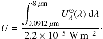 (2)The value
U = 1 corresponds to the intensity of the solar neighborhood. In these
conditions, large interstellar silicates have an equilibrium temperature of ≃17.5 K. It
is possible that the ISRF of the LMC differs from
(2)The value
U = 1 corresponds to the intensity of the solar neighborhood. In these
conditions, large interstellar silicates have an equilibrium temperature of ≃17.5 K. It
is possible that the ISRF of the LMC differs from  , since it has
younger stellar populations. This spectral shape is also likely to vary spatially within
the LMC, being harder in transparent regions, and redder in dense regions. However, as
explained previously, this will impact only the PAH and VSG spectra, which are not
determinant to estimate the total dust mass.
, since it has
younger stellar populations. This spectral shape is also likely to vary spatially within
the LMC, being harder in transparent regions, and redder in dense regions. However, as
explained previously, this will impact only the PAH and VSG spectra, which are not
determinant to estimate the total dust mass.
In the same way, we are adopting the Galactic framework, by using the grain properties of Zubko et al. (2004). We choose the bare grain model, with solar abundance constraints (BARE-GR-S). The abundance and size distribution of each grain species was constrained by fitting the IR emission, UV-visible extinction and elemental depletions of the Galactic diffuse ISM. We have updated this model with the new Draine & Li (2007) PAH optical properties, that includes more accurate band profiles, based on Spitzer spectra.
The optical properties and enthalpies considered here are summarized in Table 2. The grain cross-sections are computed using a Mie code, and following the method of Laor & Draine (1993, Sect. 2.2; Appendix A. The temperature fluctuations are computed for each grain size of each component, and for each starlight intensity, using the transition matrix method (Guhathakurta & Draine 1989).
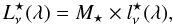
The specific monochromatic luminosity of a mass element of ISM exposed to the starlight
intensity U is:  (3)where
fPAH, fcarb and
fsil are the mass fractions of PAHs (charge fraction of
1/2), graphite and silicate
(fPAH + fcarb + fsil = 1),
and
(3)where
fPAH, fcarb and
fsil are the mass fractions of PAHs (charge fraction of
1/2), graphite and silicate
(fPAH + fcarb + fsil = 1),
and  ,
,
 ,
,
 are the corresponding size
distribution integrated specific monochromatic luminosities. In this paper, we keep the
mass fractions to the Galactic values (Zubko et al.
2004), except fPAH that we vary to fit the observed
IRAC8 μm band.
are the corresponding size
distribution integrated specific monochromatic luminosities. In this paper, we keep the
mass fractions to the Galactic values (Zubko et al.
2004), except fPAH that we vary to fit the observed
IRAC8 μm band.
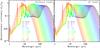 |
Fig. 1 Uniformly illuminated dust SEDs, exposed to various radiation field intensities U. Each curve represents the sum of the emission by PAH0, PAH+, carbon grains and silicates, exposed to U, in units of 2.2 × 10⁻⁵ W m-2. The monochromatic luminosity is normalised by its integrated luminosity LIR. |
Throughout this paper, we will systematically compare the two following dust compositions, in order to study a possible evolution of composition between the Milky Way and the LMC.
-
1.
“The standard model” (hereafter labeled Std) is the originalZubko et al. (2004) Galactic graincomposition, made of PAHs, graphite and silicates. The effectivesubmillimeter opacity of this dust corresponds to an emissivityindex β ≃ 2 (Appendix A).
-
2.
“The AC model” (hereafter labeled AC) is the “standard model”, but replacing graphite by amorphous carbons (ACAR; Zubko et al. 1996). This substitution is arbitrary. The purpose of this model is to test realistic compositions having a higher effective submillimeter opacity (β ≃ 1.7; Appendix A), without violating the elemental abundances.
We note that the heat capacities of amorphous carbons are unknown. We adopt those of graphite in replacement. It might be a crude approximation. However, this inconsistency will affect only the stochastically heated grains, which do not contribute significantly to the dust mass.
The individual SEDs are shown in Fig. 1. The two models show similar features.
-
1.
The far-IR peak is dominated by grains in thermal equilibriumwith the radiation field. Their spectrum is roughly a modifiedblack body. The peak wavelength of the emission shifts to shorterwavelengths when U rises, as the equilibrium temperature rises.
-
2.
The mid-IR continuum, for U ≲ 104, is dominated by small grains (radius a ≲ 0.01μm) and PAHs (prominent emission bands at 3.3, 6.2, 7.7, 8.6, 11.3 μm), both out of equilibrium with the radiation field. These grains are being heated by single photon events and the spectral shape of their emission is independent of U. Their spectrum normalized to LIR (or U) is constant. The change of shape of the mid-IR spectrum with U is only due to the contribution of equilibrium grains at these wavelengths, when their temperature reaches Teq ≳ 80 K (U ≳ 104). In particular, the prominent 9.7μm silicate feature in emission dominates the mid-IR wavelengths, in this temperature regime.
3.3. Synthetic multi-environment SED
Each SED we model in this paper is likely to be the combination of the emission from regions with different physical conditions. To account for this diversity of conditions, we make the following assumptions.
-
1.
We assume that the dust properties are uniform within themodelled region: the size distribution, and mass fractions areconstant. Only the starlight intensity varies. This is anapproximation. We will discuss in Sect. 4.3.6potential local variations of the grain properties.
-
2.
The distribution of starlight intensities per unit dust mass, throughout the region, can be approximated by a power-law (Dale et al. 2001):
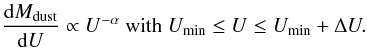 (4)This is an
empirical prescription. Dale et al. (2001,
Sect. 5.5) provide a physical justification of this formulation. However,
its main advantage is that it allows for flexible parametrizing of the physical
conditions. A more complex formulation is discussed in Appendix C.1.
(4)This is an
empirical prescription. Dale et al. (2001,
Sect. 5.5) provide a physical justification of this formulation. However,
its main advantage is that it allows for flexible parametrizing of the physical
conditions. A more complex formulation is discussed in Appendix C.1.
The total dust mass of each modelled region is therefore: 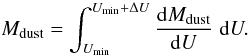 (5)In addition, to
subtract the stellar contribution from the mid-IR bands, we add a stellar continuum,
parametrized by the stellar mass in the region
M ⋆ :
(5)In addition, to
subtract the stellar contribution from the mid-IR bands, we add a stellar continuum,
parametrized by the stellar mass in the region
M ⋆ :
 (6)where
 is the specific monochromatic
luminosity of a 1 Gyr stellar population, synthesized with the model PEGASE (Fioc & Rocca-Volmerange 1997). Since, this
population is constrained mainly by the IRAC3.6 μm and
IRAC4.5 μm bands, the age of the populations do not have a
big effect. On the other hand, this stellar mass is poorly determined and should not be
trusted. The only purpose of this component is to give a better
χ2. To accurately determine the mass of the stellar
populations, we would need to take into account shorter wavelengths. This is not the
purpose of this paper.
is the specific monochromatic
luminosity of a 1 Gyr stellar population, synthesized with the model PEGASE (Fioc & Rocca-Volmerange 1997). Since, this
population is constrained mainly by the IRAC3.6 μm and
IRAC4.5 μm bands, the age of the populations do not have a
big effect. On the other hand, this stellar mass is poorly determined and should not be
trusted. The only purpose of this component is to give a better
χ2. To accurately determine the mass of the stellar
populations, we would need to take into account shorter wavelengths. This is not the
purpose of this paper.
In summary, the total monochromatic luminosity of the model is: 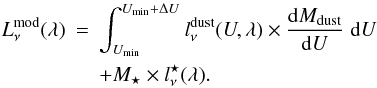 (7)For
each waveband λi, where the observed
monochromatic luminosity is
(7)For
each waveband λi, where the observed
monochromatic luminosity is  , we compute the synthetic
photometry,
, we compute the synthetic
photometry,  , by convolving the model
with the instrumental spectral response, using the appropriate conventions provided by the
user’s manuals of each instrument. We minimize the χ2, using a
Levenberg-Marquart algorithm (Press et al. 1992).
The χ2 is weighted as follows:
, by convolving the model
with the instrumental spectral response, using the appropriate conventions provided by the
user’s manuals of each instrument. We minimize the χ2, using a
Levenberg-Marquart algorithm (Press et al. 1992).
The χ2 is weighted as follows: 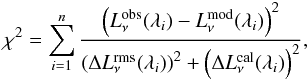 (8)where
 and
and
 are respectively the rms
and calibration errors of the waveband centered at wavelength
λi (see Sect. 3.4). We do not use the SPIRE500 μm flux as
a constraint, because of its excess relative to the model, as discussed by Gordon et al. (2010). Instead, we will study the
behaviour of this excess in Sect. 4.4, in order to
attempt to decipher its origin.
are respectively the rms
and calibration errors of the waveband centered at wavelength
λi (see Sect. 3.4). We do not use the SPIRE500 μm flux as
a constraint, because of its excess relative to the model, as discussed by Gordon et al. (2010). Instead, we will study the
behaviour of this excess in Sect. 4.4, in order to
attempt to decipher its origin.
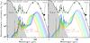 |
Fig. 2 Decomposition of the integrated strip SED into the individual uniformly illuminated
SEDs. The grey circles and error bars are the integrated observed fluxes of R10
(Table 1). The total model (black line;
Eq. (7)) is the sum of the
independent stellar component (grey filled area), and of the integral of uniformly
illuminated dust SEDs (in colors; Eq. (4)). There is linear gradation in U between colors for
the uniformly illuminated SEDs. The starlight intensity U is in
units of 2.2 × 10⁻⁵ W m-2. The sum of these components is the
black line. The green dots are the synthetic photometry (i.e. the model integrated
in each instrumental filter). The left panel shows the
“standard model”, while the right panel shows
the “AC model”. To quantify the quality of the fits, the reduced
chi square is |


Figure 2 demonstrates this model on the integrated strip SED (R10). The two panels highlight the degeneracy between the starlight intensity distribution and the submillimeter opacities, by comparing the fit of the two compositions to the same observations. Having a flatter submillimeter opacity gives a fit with less massive, hotter dust populations.
Parameters of the model.
rms values for each filter and each spatial resolution.
Table 3 summarizes the parameters of the model. In
particular, the last column of Table 3 describes
the behaviour of the free parameters. When an SED fit is performed, a slight variation of
one parameter value, due to observational errors, may systematically be compensated by the
variation of another parameter. Although the free parameters are rigorously independent,
this effect may induce a correlation between these parameters. The Monte-Carlo error
analysis that will be discussed in Sect. 3.4.2 is a
good way to quantify these correlations. The most striking example, in our case, is the
correlation between the three parameters controlling the starlight intensity distribution
(α, Umin and ΔU;
Eq. (4)). Moreover, these parameters do
not have a physical meaning. Rather than discussing their values, it is more convenient to
consider the first two moments of the starlight intensity distribution:
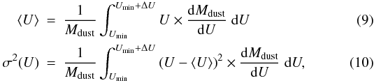 which
develop into:
which
develop into: 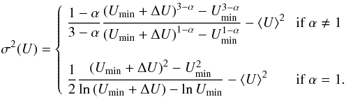 (11)and:
 (12)We
define the infrared luminosity as the power emitted by the dust:
(12)We
define the infrared luminosity as the power emitted by the dust:  (13)Finally, the
“gas-to-dust mass ratio” is the ratio of the total mass of gas
(H i and H2, with helium and heavy elements) to the total dust mass,
in the same region:
(13)Finally, the
“gas-to-dust mass ratio” is the ratio of the total mass of gas
(H i and H2, with helium and heavy elements) to the total dust mass,
in the same region:  (14)For comparison,
the Galactic value is (Zubko et al. 2004):
(14)For comparison,
the Galactic value is (Zubko et al. 2004):
 (15)It is important to
note that, for the discussion in Sect. 4, this value
is consistent with the dust properties we use. Moreover, this model is consistent with the
elemental depletion constraints.
(15)It is important to
note that, for the discussion in Sect. 4, this value
is consistent with the dust properties we use. Moreover, this model is consistent with the
elemental depletion constraints.
3.4. Rigorous error propagation
Since our dust model is highly non-linear, it is crucial to rigorously propagate the observational errors through the entire fitting procedure, taking into account the fact that some errors are independent and others are correlated. In this way, we will be able to quote consistent errors on the parameters. We first need to identify the various sources of error
3.4.1. Sources of observational error
For each wavelength, at each spatial resolution, we measure the noise of the map by taking the standard deviation of the pixel values in what is considered to be the background, i.e. the upper and lower ends of the strip. These values are given in Table 4. These errors are independent from one wavelength to the other, and from one pixel to the other. A simple check of the distribution of pixel values shows that the uncertainty is well described by a Gaussian.
The calibration error is the error on the flux conversion factor. This error is therefore correlated between each pixel. It can be synthesized as follows.
-
IRAC:
the 1σ calibration uncertainty is σcal(IRAC) = 2% (Reach et al. 2005). The different wavelengths are correlated.
-
MIPS24 μm:
Engelbracht et al. (2007) quote a 1σ calibration error of σcal(MIPS24 μm) = 4%. It is independent of the other wavebands.
-
MIPS70 μm:
Gordon et al. (2007) quote a 1σ calibration error of σcal(MIPS70 μm) = 5% for the coarse scale mapping used for the SAGE observations.
-
MIPS160 μm:
Stansberry et al. (2007) report a 1σ calibration error of σcal(MIPS160 μm) = 12%. This error is correlated with the MIPS70 μm error.
-
Although Swinyard et al. (2010) report a calibration error of σcal(SPIRE) = 15%, it is necessary to decompose this error into its components (SPIRE consortium 2010), as the SPIRE fluxes are the most crucial constraints on the dust mass and emissivity.
-
1.
The 3σ error on the calibration model is
 , each waveband being correlated.
 -
2.
The noise in the calibration observations (Ceres) are:
-
 (SPIRE250 μm) = 7%;
 -
(SPIRE350 μm)
= 12%;
-
(SPIRE500 μm)
= 6%.
-
-
3.
The error on the beam area are
 and
they are independent.
and
they are independent.
-
1.
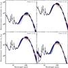 |
Fig. 3 Demonstration of the Monte-Carlo method on the 4 pixels of the R9 map. The grey ellipses represent the unperturbed observations and their uncertainties: the filter band widths on the x direction; the ± 1σ error bars on the y direction (dark grey); and the ± 3σ error on the y direction (concentric light grey ellipse). The color lines show the NMC = 300 model fits to the perturbed fluxes. We used the “standard model” for the demonstration. Some points (like MIPS70 μm) appears shifted from the models because of the color correction. The two shortest wavelengths of the [1,4] pixel are poorly fitted since the IRAC3.6 μm is only an upper limit. This might be the result of oversubtraction of point sources in this low surface brightness region. However, this discrepancy affects only the level of the independent stellar contribution. It does not affect the longer wavelength fit. |
3.4.2. Monte-Carlo iterations
We propagate the observational errors detailed in Sect. 3.4.1, by performing Monte-Carlo iterations of each fit. More precisely, for each observed SED, we perform a large number (NMC ≃ 300) of fits of the SED with additional random perturbations. Figure 3 demonstrates the fits of the perturbed SEDs of the 4 pixels of the R9 map. Each model corresponds to one particular set of random perturbations. These perturbations take into account the two main sources of errors, as follows.
-
1.
The pixel noise at each wavelength (Sect. 4) isassumed to be a normal random independent variable. The noiseis independent from one pixel to the other.
-
2.
The calibration error is assumed to be a normal random variable, with standard deviation and correlation between wavelengths as described in Sect. 3.4.1. The calibration error from one pixel to the other is correlated.
From a technical point of view, we generate the complete set of independent random variables necessary for the calibration errors, and keep them for our entire analysis. Indeed, one of the advantages of the Monte-Carlo technique is that it allows us to account for complex correlations between variables. As will be demonstrated in Sect. 4.2, the error on the ratio of two quantities depending on the calibration error is often lower than the errors on each individual quantity. It is due to the fact that the calibration error cancels when considering a relative quantity. It is even possible to take this effect into account when comparing the results of two different models, as will be shown in Sect. 4.1.
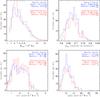 |
Fig. 4 Distribution of the main parameters of the perturbed SED fits of the four R9 pixels (Fig. 3). For each parameter, we show the number of Monte-Carlo fits to the perturbed SED per bin of parameter value. The value of each parameter, for a given iteration is the combination of the values of the parameter for each of the 4 pixels. We quote both the mean and the median. The blue distributions correspond to the rigorous Monte-Carlo statistics, while the red distributions are from our reconstruction method (Appendix B). |
Figure 4 shows the statistical distributions of the main model parameters, corresponding to the fits of Fig. 3. The parameter value of each Monte-Carlo iteration is the sum of the parameter value of each pixel. The first panel of this figure demonstrates, in particular, that the dust mass has a ≃50% uncertainty, even for very high signal-to-noise ratio SEDs. In addition it clearly shows the asymmetry of the distribution, which is a result of the non-linearity of the model. The upper end of the statistical distribution of dust masses is less constrained than the lower end, because of the non-linear dependence of the dust mass with the temperature.
Even with a fast running model, computing NMC ≃ 300 fits for each pixel is CPU intensive, and not necessary. Instead, we use an approximation to reconstruct the probability distributions of each parameter. This method is detailed in Appendix B. It consists of interpolating the pre-computed errors of 30 classes of SEDs, parametrized by their specific power (LIR/Mdust) and the rms level. Figure 4 compares this reconstruction method to the rigorous Monte-Carlo results. It succeeds in reproducing the correct central value and errors. In particular, it reproduces accurately the skewness of the probability distribution.
3.4.3. Error display
Throughout this paper, each time a numerical quantity is reported as
X ≃ a ± b, the two quantities
a and b will refer to the mean and standard
deviation, or in other words: 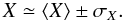 (16)On the other hand, for
numerical quantities having a strongly asymmetric distribution, we will quote the error
as
(16)On the other hand, for
numerical quantities having a strongly asymmetric distribution, we will quote the error
as  .
Only in this case will the quantities refer to the three quartiles,
Q1(X),
Q2(X),
Q3(X), corresponding to values of the
repartition function of 1/4, 1/2 and 3/4, respectively:
.
Only in this case will the quantities refer to the three quartiles,
Q1(X),
Q2(X),
Q3(X), corresponding to values of the
repartition function of 1/4, 1/2 and 3/4, respectively: ![Mathematical equation: \begin{equation} X\simeq Q_2(X)_{\displaystyle-[Q_2(X)-Q_1(X)]}^{\displaystyle+[Q_3(X)-Q_2(X)]}. \label{eq:median} \end{equation}](/articles/aa/full_html/2011/12/aa17952-11/aa17952-11-eq269.png) (17)The latter error
(Eq. (17)) corresponds to a confidence
level of 50%, by definition. It is also interesting to consider a higher confidence
interval. Most of our error estimates are based on NMC = 300
Monte-Carlo iterations. It would therefore be meaningless to go down to less than
1/
(17)The latter error
(Eq. (17)) corresponds to a confidence
level of 50%, by definition. It is also interesting to consider a higher confidence
interval. Most of our error estimates are based on NMC = 300
Monte-Carlo iterations. It would therefore be meaningless to go down to less than
1/ % error tolerance. We
therefore choose to quote the 90% confidence level, defined by the range of the
parameter values between 0.05 and 0.95 of the repartition function. From a technical
point of view, with NMC = 300, the limits of this interval
are simply the 15th and 286th ordered Monte-Carlo parameter values. We will note this
interval:
% error tolerance. We
therefore choose to quote the 90% confidence level, defined by the range of the
parameter values between 0.05 and 0.95 of the repartition function. From a technical
point of view, with NMC = 300, the limits of this interval
are simply the 15th and 286th ordered Monte-Carlo parameter values. We will note this
interval: ![Mathematical equation: \begin{equation} X \simeq [X_{\rm inf},X_{\rm sup}]_{90\%}. \label{eq:sup} \end{equation}](/articles/aa/full_html/2011/12/aa17952-11/aa17952-11-eq272.png) (18)On figures, the
50% error bars will be displayed with a solid line, and the 90% interval with a dashed
line.
(18)On figures, the
50% error bars will be displayed with a solid line, and the 90% interval with a dashed
line.
We note that taking the median (Eq. (17)) gives a central value very close to the best fit, while taking the mean (Eq. (16)) gives a central value systematically shifted from the best fit. Figure 4 demonstrates this effect: the best fit value of the dust mass is 8.62 × 10⁵ M⊙, very close to the median of the Monte-Carlo iterations (8.76 × 10⁵ M⊙). On the contrary, the mean, 1.03 × 10⁶ M⊙, is significantly higher. This is due to the skewness of the probability distribution of the parameter values.
4. The dust mass estimate and its uncertainties
4.1. Systematic discrepancies between the two models
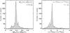 |
Fig. 5 Comparison between the parameters obtained with the two models. The left panel shows the statistical distribution of the pixel-to-pixel dust mass ratio between the “AC model” and the “standard model” at spatial resolution R4. The right panel shows a similar ratio for the mass averaged starlight intensity ⟨ U ⟩ . |
We have applied the model presented in Sect. 3, with
the two compositions (“standard” and “AC”), to the maps
listed in Table 1. The dust mass spatial
distribution obtained with the two models are very similar. Figure 5 shows the distribution of the pixel-to-pixel ratio of the dust masses
(“standard” over “AC” models), and starlight
intensities, at spatial resolution R4. These distributions are very tight. It shows, that
the dust masses obtained with the “AC model” are systematically lower by
a factor of  than dust masses obtained with the “standard model”, while the starlight
intensities are systematically higher by a factor of
than dust masses obtained with the “standard model”, while the starlight
intensities are systematically higher by a factor of
 .
These parameters are tied together. Grains with the “AC model” absorb
more light than grains of the “standard model” (Appendix A). They therefore require less mass to account for the
observed IR luminosity.
.
These parameters are tied together. Grains with the “AC model” absorb
more light than grains of the “standard model” (Appendix A). They therefore require less mass to account for the
observed IR luminosity.
Thus, the results derived with the two compositions give similar trends, but the absolute value of their parameters systematically differ.
4.2. Bias originating in the lack of spatial resolution
 |
Fig. 6 Trend of the total dust mass with spatial resolution. The left panels show the trends for the “standard model”, while the right panels show the trends for the “AC model”. For each panel, the x-axis is the spatial resolution of the maps used to derive the dust mass. Each point of the trends corresponds to one of the maps listed in Table 1. For the two top panels, the y-axis is the total dust mass. This mass is the sum of the dust mass of each pixel. For each resolution, there are as many SED fits as the number of pixels listed in Table 1. The two bottom panels show the relative dust mass variation. It is normalized by the integrated strip (R10). In that way, the calibration errors cancel, and the trend has smaller error bars. The dashed error bars display the 90% confidence interval. |
In order to quantify the effect of the non-linearity of our SED model, we compute the total dust mass for each map listed in Table 1, with our two grain compositions. Figure 6 shows the resulting trends of dust mass with spatial resolution. These trends are shown for both models. The mass at each resolution is the sum of the masses of all defined pixels. The top panels show the trend of the absolute value of the dust mass. The trends look similar for both models. They appear systematically shifted as discussed in Sect. 4.1. The error bar on each value is large and covers roughly the range of the trend. However, the relative variation of the dust mass (bottom panels of Fig. 6) has significantly smaller error bars. These trends are obtained by normalizing each one of the NMC Monte-Carlo results of a given spatial resolution, by the corresponding mass for the integrated strip (R10). In that way, most of the calibration error cancels. The only remaining source of uncertainty is the intercalibration error between the various instruments and the rms noise. The dynamics of the trend is unchanged.
The relative trends of Fig. 6 show that measuring the dust mass of an integrated galaxy can give significantly lower values than performing fits of its spatially resolved regions, providing that the spatial resolution is fine enough. For the LMC, the spatially resolved dust mass estimate is ≃50% higher than the integrated SED fit. This variation is not due to the noise, since the error bars are much smaller than the spread of the trend. Thus, the true mass is probably closer to the high spatial resolution value (R1) than to the integrated flux value (R10). It appears that there is a spatial scale where the trend stabilizes. This transition is an optimal resolution for our model, as it probably provides a correct dust mass, and the noise is lower than at R1. This optimal spatial scale corresponds to R3–R4 (≃27–54 pc; Table 1).
The origin of this trend likely lies in the morphology of the ISM. It could be the result of the dilution of cold massive regions in hotter regions. It is possible that there is a typical spatial scale below which most of the cold regions dominate the SED of the pixels where they lie. It may correspond to the typical scale of molecular complexes. With only a few far-IR/submm constraints, it is difficult to account for these regions when modelling the integrated SED.
To demonstrate the origin of this trend, Fig. 7
compares the pixel distribution of the dust mass surface density, at two spatial
resolutions. Taking into account the statistical fluctuations, due to the low pixel number
of R7, the two distributions (R1 and R7) agree at low dust mass surface densities
( ).
However, at high dust mass surface densities (
).
However, at high dust mass surface densities ( ),
there is a higher fraction of pixels for the high resolution map. This fraction is
compensated by an excess of intermediate surface density pixels at low spatial resolution
(
),
there is a higher fraction of pixels for the high resolution map. This fraction is
compensated by an excess of intermediate surface density pixels at low spatial resolution
( ).
Thus, the origin of the dust mass underestimation is due to the inability of our model to
probe dense regions, at low spatial resolutions. At these spatial resolutions, the mass
and average temperature of cold regions are biased by the contribution from hot regions
present in the same beam, as the latter are more emissive. On the other hand, at high
spatial resolution, cold regions tend to be better separated from hot regions and can
therefore be modelled more accurately.
).
Thus, the origin of the dust mass underestimation is due to the inability of our model to
probe dense regions, at low spatial resolutions. At these spatial resolutions, the mass
and average temperature of cold regions are biased by the contribution from hot regions
present in the same beam, as the latter are more emissive. On the other hand, at high
spatial resolution, cold regions tend to be better separated from hot regions and can
therefore be modelled more accurately.
4.3. The gas-to-dust mass ratio crisis: several competitive scenarios
4.3.1. Metal abundance constraints
To be rigorous, we first need to estimate the uncertainty on the metallicity of the LMC. Pagel (2003) compiles the literature for numerous elemental abundances in different regions of the LMC and of the Galaxy. We estimate the error on each element of Table 1 of Pagel (2003), by taking the dispersion of the different measures, excluding cepheids which are very dispersed and not available for all elements. These uncertainties are summarized in Table 5.
Literature compilation for the elemental abundances.
We assume that we can reliably derive the metallicity by scaling the mass of O, C and
N. In particular, this is supported by the fact that O and C are the major dust
constituents. The metallicity of the LMC we adopt is thus: 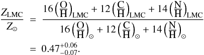 (19)This
estimate is more accurate than simply scaling the oxygen abundance, as it is usually
done.
(19)This
estimate is more accurate than simply scaling the oxygen abundance, as it is usually
done.
Let’s check the physical consistency of our dust masses. The Galactic gas-to-dust mass
ratio is  (Zubko et al. 2004). We emphasize that this
value is consistent with the elemental depletion patterns. Assuming that the dust-to-gas
mass ratio scales with metal abundance (i.e. the dust-to-metal mass ratio is constant),
the expected gas-to-dust mass ratio for the LMC is:
(Zubko et al. 2004). We emphasize that this
value is consistent with the elemental depletion patterns. Assuming that the dust-to-gas
mass ratio scales with metal abundance (i.e. the dust-to-metal mass ratio is constant),
the expected gas-to-dust mass ratio for the LMC is: 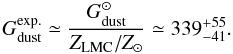 (20)Assuming that the
mass fraction of gaseous heavy elements in the Galaxy is
Z⊙ ≃ 0.017 (Grevesse
& Sauval 1998), the solar metallicity dust-to-metal mass ratio is:
(20)Assuming that the
mass fraction of gaseous heavy elements in the Galaxy is
Z⊙ ≃ 0.017 (Grevesse
& Sauval 1998), the solar metallicity dust-to-metal mass ratio is:
 (21)It is
therefore difficult to understand how the gas-to-dust mass ratio in the LMC could be
lower than:
(21)It is
therefore difficult to understand how the gas-to-dust mass ratio in the LMC could be
lower than:  (22)without requiring
a larger amount of metals locked-up in grains than what is available in the ISM. These
values are summarized in Table 6.
(22)without requiring
a larger amount of metals locked-up in grains than what is available in the ISM. These
values are summarized in Table 6.
Reference metallicity and gas-to-dust mass ratios.
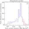 |
Fig. 7 Pixel distribution of the dust mass surface density for two spatial resolutions. We plot only the “standard model”. The figure is qualitatively similar for the “AC model”. The distributions are normalized. It shows that, at lower spatial resolution, the very high surface densities are missed (red filled area), and there is an excess of intermediate surface densities (blue filled area). |
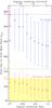 |
Fig. 8 Consistency of the gas-to-dust mass ratios. The two trends show the gas-to-dust
mass ratio as a function of the spatial resolution, for each model. We also
display the 90% confidence interval for the “standard model”,
with dashed lines. The yellow and purple error bars, with the star symbol,
represent the uncertainities on |

4.3.2. Preliminary: global analysis
Total gas-to-dust mass ratio, as a function of the spatial resolution, for the two models.
Table 7 shows the gas-to-dust mass ratio at each
spatial resolution for the two models. These ratios are displayed in Fig. 8. The total gas-to-dust mass ratios given by the
“standard model” are too low by a factor of
![Mathematical equation: \hbox{$G_{\rm dust}^{\rm exp.}/G_{\rm dust}^{\rm Std}({\rm R1})\simeq3.8_{-1.0}^{+1.7}\simeq[2.1,9.7]_{90\%}$}](/articles/aa/full_html/2011/12/aa17952-11/aa17952-11-eq352.png) .
They are even lower than the physical limit by a factor of
.
They are even lower than the physical limit by a factor of
![Mathematical equation: \hbox{$G_{\rm dust}^{\rm lim.}/G_{\rm dust}^{\rm Std}({\rm R1})\simeq1.4_{-0.4}^{+0.6}\simeq[0.8,3.6]_{90\%}$}](/articles/aa/full_html/2011/12/aa17952-11/aa17952-11-eq353.png) .
We emphasize here that there is no spatial correlation between the foreground Galactic
H i column density (Sect. 2.1) and the
gas-to-dust mass ratio deficit of the “standard model”. Therefore, the
residual cirrus emission is not responsible for this deficit. Statistically, the
“standard model” violates the elemental abundances with a probability
of 80%, while the “AC model” is consistent. Therefore, if we assume
that our gas mass is correct, then we can conclude that the properties of the
“standard model” do not apply to the LMC. This is one scenario.
.
We emphasize here that there is no spatial correlation between the foreground Galactic
H i column density (Sect. 2.1) and the
gas-to-dust mass ratio deficit of the “standard model”. Therefore, the
residual cirrus emission is not responsible for this deficit. Statistically, the
“standard model” violates the elemental abundances with a probability
of 80%, while the “AC model” is consistent. Therefore, if we assume
that our gas mass is correct, then we can conclude that the properties of the
“standard model” do not apply to the LMC. This is one scenario.
However, there is a second scenario: the discrepant gas-to-dust mass ratio obtained with the “standard model” could result from the underestimate of the total gas mass. In particular, the mass of molecular gas could have been underestimated. It is known that in low-metallicity environments, the H2 gas is not properly traced by 12CO(J = 1 → 0)2.6 mm. In these environments, the CO cores are thought to be much smaller relative to their H2 envelope (H2 being more efficiently self-shielded). This scenario is supported by the exceptionally high observed [C ii]158 μm/12CO(J = 1 → 0)2.6 mm luminosity ratio in dwarf galaxies (e.g. [C ii]158 μm/12CO(J = 1 → 0)2.6 mm ≃ 20 000 in the LMC, compared to [C ii]158 μm/12CO(J = 1 → 0)2.6 mm ≃ 4000 in normal metallicity galaxies; Poglitsch et al. 1995; Israel 1997; Madden et al. 1997; Madden 2000). In principle, the underestimation of the molecular gas mass, using the CO line, could be a factor of ≃10−100, in these environments (Madden et al. 2011).
Let’s assume that our dust properties are correct, and that
 is very
low due to having underestimated the molecular gas mass. Noting
is very
low due to having underestimated the molecular gas mass. Noting
 the correction factor accounting for the hypothetical molecular gas not traced by CO and
for the fact that our XCO conversion factor (Sect. 2.3) might be wrong, the total gas-to-dust mass ratio
would have to be:
the correction factor accounting for the hypothetical molecular gas not traced by CO and
for the fact that our XCO conversion factor (Sect. 2.3) might be wrong, the total gas-to-dust mass ratio
would have to be: ![Mathematical equation: \begin{eqnarray} \frac{M_{\rm gas}^{\rm \hi}+\mathcal{C}_{\rm H_2}M_{\rm gas}^{\rm H_2}}{M_{\rm dust}^{\rm Std}({\rm R1})} & = & G_{\rm dust}^{\rm exp.} \\ \Rightarrow \mathcal{C}_{\rm H_2} & \simeq & 10.1_{-3.6}^{+5.9} = [4.0,30.6]_{90\%}. \nonumber \end{eqnarray}](/articles/aa/full_html/2011/12/aa17952-11/aa17952-11-eq361.png) (23)In
other words, to explain the discrepant gas-to-dust mass ratio of the “standard
model”, we would have to conclude that the molecular gas mass would have been
globally underestimated by at least one order of magnitude.
(23)In
other words, to explain the discrepant gas-to-dust mass ratio of the “standard
model”, we would have to conclude that the molecular gas mass would have been
globally underestimated by at least one order of magnitude.
These two alternative scenarios are degenerate, when considering only global values. We therefore need to take into account the redundancy provided by the spatial distribution of the gas-to-dust mass ratio, in order to sort these scenarios out.
4.3.3. Spatial distribution of the gas-to-dust mass ratio
Figure 9 shows the map of IR luminosity for the “standard model”. Since this quantity is the integration of the interpolated observed SED, it depends very little on the model; LIR distribution of the “standard model” looks almost identical to the “AC model”. That is the reason why we displayed it only for the “standard model”. The upper panels of Fig. 10 show the spatial distribution of the gas-to-dust mass ratio with the two models. A few regions at the two ends of the strip exhibit noisy pixels. They correspond to very low surface densities. In general, there is no particular spatial correlation between the gas-to-dust mass ratio and the CO concentrations. The lower panels of Fig. 10 show the corresponding map of the mass averaged starlight intensity ⟨ U ⟩ , for both models.
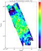 |
Fig. 9 Spatial distribution of the IR luminosity, for the “standard model”, at resolution R4 (54 pc). The color image represents the IR luminosity map. The color scale is logarithmic. The white contours show the main CO concentrations from the Nanten map (Fukui et al. 2008). This contour level is chosen so that 90% of the CO mass has a higher column density than this level. In other words, 90% of the CO mass is in these concentrations. The map is almost rigorously identical with the “AC model”. |
Figure 11 shows the pixel-to-pixel distribution
of Gdust for the highest spatial resolution where the gas
maps are defined (R4). It appears that the distribution for the “standard
model” is shifted to lower values, the pixels are systematically too low,
compared to the expected value. In addition, we have built a histogram of the pixels
below an arbitrary column density ( and
and 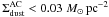 ),
in the two lower panels of Fig. 11. We have
defined the surface densities at a given spatial resolution by dividing the mass in the
pixel by the area of this pixel (Table 1):
),
in the two lower panels of Fig. 11. We have
defined the surface densities at a given spatial resolution by dividing the mass in the
pixel by the area of this pixel (Table 1):
 . The two
lower panels of Fig. 11 demonstrate that most of
the pixels exhibiting high gas-to-dust mass ratios are located in regions of low dust
column density, independently of the model used.
. The two
lower panels of Fig. 11 demonstrate that most of
the pixels exhibiting high gas-to-dust mass ratios are located in regions of low dust
column density, independently of the model used.
 |
Fig. 10 Spatial distribution of the main dust parameters, for the two models, at resolution R4 (54 pc). The color images of the two upper panels represent the gas-to-dust mass ratio map, for each model. The color images of the two lower panels represent the mass averaged starlight intensity map, for each model. The color scale is logarithmic. The white contours show the main CO concentrations from the Nanten map (Fukui et al. 2008). This contour level is chosen so that 90% of the CO mass has a higher column density than this level. In other words, 90% of the CO mass is in these concentrations. |
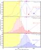 |
Fig. 11 Pixel-to-pixel distribution of the gas-to-dust mass ratio for R4 (54 pc). The two
histograms of the top panel are the pixel probability
distribution of the gas-to-dust mass ratio for the two models. The spread of the
distribution reflects the pixel to pixel spread fluctuations of the ratio. The
actual error on the total Gdust is smaller than this
spread (Table 7). For comparison, we show
the values of |
Regarding this property, we need to study the variations of the gas-to-dust mass ratio as a function of surface density.
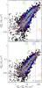 |
Fig. 12 Correlation between the gas and dust mass column densities. Each panel
corresponds to a model. The spatial resolution is R4 (54 pc). The colored area is
the pixel density. The number density of pixels for each
[Σgas,Σdust] values is coded with the
same color scale as in Fig. 13. The circles
with error bars show the binned trend. The horizontal error bar displays the
Σgas bin width. The vertical error bar displays the dispersion in
Σdust within each Σgas bin. The Σgas bin sizes
are chosen so that each bin contains the same number of pixels. The red line is
the best fit of Eq. (24) to the
binned trend. The vertical lines show the best fit values
|

4.3.4. The correlation between gas and dust column densities
In this section, we analyze the correlation between gas and dust using a method similar
to that of Planck Collaboration et al. (2011b).
It is aimed at identifying the presence of “dark gas” (hereafter
DG)1, as a departure from the linear correlation
between gas and dust. We have defined bins of gas mass surface density
( ),
so that the same number of pixels falls within each bin. We have then computed the
average value and the scatter of the dust mass of the pixels within each bin.
Figure 12 shows this binned trend on top of the
pixel density plot. The binned dust mass surface density is fit with the following
function:
),
so that the same number of pixels falls within each bin. We have then computed the
average value and the scatter of the dust mass of the pixels within each bin.
Figure 12 shows this binned trend on top of the
pixel density plot. The binned dust mass surface density is fit with the following
function:
 (24)where
the free parameters are the following.
(24)where
the free parameters are the following.
-
 is the
fit gas-to-dust mass ratio. It assumes that the actual gas-to-dust mass ratio is
the same everywhere in the LMC.
is the
fit gas-to-dust mass ratio. It assumes that the actual gas-to-dust mass ratio is
the same everywhere in the LMC. -
 is the
fit correction factor of the assumed XCO. Since we
have assumed
XCO = 7 × 10²⁰H cm-2 (K km s-1)-1
(Sect. 2.3), then the value of the fit
conversion factor is
is the
fit correction factor of the assumed XCO. Since we
have assumed
XCO = 7 × 10²⁰H cm-2 (K km s-1)-1
(Sect. 2.3), then the value of the fit
conversion factor is  .
.
-
 accounts for a possible offset in the gas mass surface density compared to the
dust mass surface density.
accounts for a possible offset in the gas mass surface density compared to the
dust mass surface density. -
 is the gas
mass surface density above which the dark gas contributes.
is the gas
mass surface density above which the dark gas contributes. -
 is the gas
mass surface density above which the molecular gas is reliably traced by
12CO(J = 1 → 0)2.6 mm, and the dark gas
therefore does not contribute anymore. Above this value, the molecular phase is
not “dark” anymore.
is the gas
mass surface density above which the molecular gas is reliably traced by
12CO(J = 1 → 0)2.6 mm, and the dark gas
therefore does not contribute anymore. Above this value, the molecular phase is
not “dark” anymore.
Equation (24) is not fit between
and
, where the
dark gas is assumed to contribute. The total dark gas mass is computed as the difference
between the binned trend and the fit of Eq. (24). It is noted  .
.
Figure 12 shows the trend and the best fit for
each model. Although the departure between the line fit and the binned trend, in the
![Mathematical equation: \hbox{$[\Sigma_{\rm gas}^{\rm DG},\Sigma_{\rm gas}^{\rm CO}]$}](/articles/aa/full_html/2011/12/aa17952-11/aa17952-11-eq378.png) is visible, its deviation is
lower than the typical dispersion of the correlation. However, the parameter values and
their uncertainties, given in Table 8, show this
departure is significant. It appears that the gas-to-dust mass ratios derived from these
simple fits are consistent with the pixel-to-pixel values (Table 7). Therefore, this analysis tends to confirm that the
“standard model” violates elemental abundances in the LMC, while the
“AC model” is physically valid. The fact that the parameter
is
consistent with unity indicates that our adopted XCO
conversion factor
(XCO = 7 × 10²⁰H cm-2 (K km s-1)-1;
Sect. 2.3) is probably not incorrect. Finally,
the dark gas mass fraction, around 10%, seems to be moderate.
is visible, its deviation is
lower than the typical dispersion of the correlation. However, the parameter values and
their uncertainties, given in Table 8, show this
departure is significant. It appears that the gas-to-dust mass ratios derived from these
simple fits are consistent with the pixel-to-pixel values (Table 7). Therefore, this analysis tends to confirm that the
“standard model” violates elemental abundances in the LMC, while the
“AC model” is physically valid. The fact that the parameter
is
consistent with unity indicates that our adopted XCO
conversion factor
(XCO = 7 × 10²⁰H cm-2 (K km s-1)-1;
Sect. 2.3) is probably not incorrect. Finally,
the dark gas mass fraction, around 10%, seems to be moderate.
There are several hypotheses entering into Eq. (24). First, its interpretation implicitly relies on the translation
between Σdust and AV, the
extinction magnitude in V band, because it defines the limits on the
dark gas regime ( and
;
Eq. (24)). However, at the spatial
scales considered here (54 pc), molecular clouds are not resolved, and several phases
are mixed within each pixel. Therefore, the dust mass surface density is in principle a
biased estimator of the AV. The value of
AV derived from the dust mass surface
density, assuming a uniform dust distribution, is actually always going to be lower than
the AV of a molecular cloud that would lie
in the pixel. Second, the approach of Eq. (24) is a perturbative method. It is correct only if the fraction of dark gas
is small. In particular, this method would fail if dark gas was present at low
Σgas. Finally, it relies on the assumption of a uniform gas-to-dust mass
ratio throughout the entire galaxy. In fact, our Gdust
spatial distributions (Fig. 10) are not noise
maps, they contain clear structures. Moreover, our error analysis demonstrates that the
amplitude of these structures is larger than the typical error bar on an individual
pixel value. And the possible offset in background subtraction between the gas and dust
maps (estimated in Table 8) is small enough to
affect only the low surface brightness pixels. Consequently, this prompts us to further
scrutinize the observed variations of Gdust as a function of
the physical conditions.
4.3.5. Variations of the gas-to-dust mass ratio with physical conditions
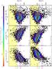 |
Fig. 13 Pixel-to-pixel correlations between various tracers of the physical conditions
and the gas-to-dust mass ratio. Results are shown for the two models, at spatial
resolution R4. The color scale represents the density of pixels in various bins of
the two parameters. The overplotted grey error bars are the trends binned over the
x-axis parameter. The bin size is defined so that the same
number of pixels falls within each bin. That is the reason why the bins are very
narrow in the center, and there are only a few points in the outer parts where the
pixel density is low. The central value is the median gas-to-dust mass ratio, and
the error bars account for the pixel-to-pixel scatter, which is similar to or
larger than the typical intrinsic error bar of a single pixel. The yellow and
purple dashed error bars, with the star symbol, represent the 90% confidence
uncertainities on |
In this section, we describe the observed trends of the gas-to-dust mass ratio as a function of several parameters. Figure 13 shows the pixel-to-pixel variations of the observed gas-to-dust mass ratio, as a function of several tracers of the physical conditions, for the two models. We note that the trends are similar with the two models, but the quantities proportional to the dust mass appear to be scaled down by a factor of ≃0.38 with the “AC model”. On the contrary, ⟨ U ⟩ appears to be scaled up by a factor of ≃2.1 (see also Fig. 5).
The two left panels of Fig. 13 show the variation of Gdust as a function of the gas mass surface density Σgas. There is a large scatter within each bin of Σgas, and the scatter is higher at low surface densities, since the signal-to-noise ratio is lower and offsets in the zero level of the gas and dust masses can impact the ratio. The gas-to-dust mass ratio at high gas mass column densities (Σgas ≳ 10 M⊙ pc-2) appears to deviate slighty from a constant value, as discussed in Sect. 4.3.4. However, this deviation is smaller than the dispersion. Overall, this trend does not show any general correlation between the gas-to-dust mass ratio and the gas mass surface density. The central values of Gdust are on average below the limit value with the “standard model”, but are found around the expected value with the “AC model”.
The two central panels of Fig. 13 show the
variation of Gdust with the dust mass surface density
Σdust. There is a clear anticorrelation between the two quantities.
Although, the trend at low surface densities
(Σdust ≲ 0.01 M⊙ pc-2) is very
scattered and sensitive to the offset (Table 8), the rest of the trend is clear. The fact that the
gas-to-dust mass ratio correlates better with the dust mass column density than with the
gas mass column density is the sign that the origin of the variations of
Gdust is not directly linked with the observed
gas content. Most of the trend is below the limit value, with the
“standard model”. On the contrary the values for the “AC
model” are all realistic.
Finally, the two right panels of Fig. 13 show the variation of Gdust with the mass averaged starlight intensity ⟨ U ⟩ . There is a clear relation between the two quantities. Contrary to the central panels (Gdust vs. Σdust), these two quantities are independent. Moreover, ⟨ U ⟩ is a specific quantity, while Σdust is integrated over the line of sight. It appears that ⟨ U ⟩ is the parameter giving the best trend with Gdust, exhibiting larger dynamics and smaller scatter than the trends with Σgas and Σdust. We note that, with both models, the slope of the correlation (in bi-logarithmic representation) is not constant. Schematically, for ⟨ U ⟩ Std ≲ 1 (or ⟨ U ⟩ AC ≲ 2), Gdust ∝ ⟨ U ⟩ . Then, for 1 ≲ ⟨ U ⟩ Std ≲ 4 (or 2 ≲ ⟨ U ⟩ AC ≲ 8), the trend flattens. There is no significant variation in this range. At larger values, Gdust ∝ ⟨ U ⟩ again, but the pixels are very dispersed in this range, and the statistics are limited.
In summary, the observed variations of Gdust do not appear to be significantly traced by the observed gas content. On the contrary, these variations are well correlated with tracers of the dust physical conditions, in particular their irradiation conditions. It suggests that the origin of these variations is linked in some way with the radiation energy density. We are now going to explore the possible interpretations of these variations.
4.3.6. Physical interpretation: dark gas, modified submm opacities or enhanced dust condensation?
To interpret the trends of Fig. 13, we need to list the possible physical processes responsible for variations of the observed gas-to-dust mass ratio, as well as the known biases affecting these trends. The known biases of our trends are the following.
-
Bias
1.
There is a potential offset between the gas and dust masszero level, due to differences in background subtractions. This offset has an impact on low surface density pixels (or high ⟨ U ⟩ ). It is quantified in Table 8.
-
Bias
2.
There is a known bias of our SED fitting. At high average starlight intensities ( ⟨ U ⟩ ≳ 10), our model tends to underestimate the dust mass. This effect is demonstrated in Fig. B.2 of Appendix B. An artificial correlation between ⟨ U ⟩ and Gdust is expected in this regime.
The possible causes of variations of the observed gas-to-dust mass ratio are the following.
-
Dark
gas.
As discussed in Sect. 4.3.2, lowGdust could be the sign of massive “dark gas” reservoir. As shown in Sect. 4.3.5, the fact that clear variations of Gdust are correlated with Σdust, but not with Σgas, suggests that the H i and CO traced gas is blind to actual variations of Gdust. Assuming that our XCO is correct, the decrease of Gdust with Σdust could be partly due to the presence of a dark gas component more massive than what was determined in Sect. 4.3.4. The latter could have been underestimated because it was lost in the scatter of the relation.
-
Dust-to-metal
ratio.
Variations of Gdust could be due to local variations of the dust-to-metal mass ratio (Eq. (21 )). In principle, the gas-to-dust mass ratio could go down to
 (Eq. (22))
and go up to infinity. Assuming an efficient mixing of freshly formed
dust grains throughout the ISM, an increase of Gdust
would
be the sign of an enhanced destruction, mainly by SN blastwaves. This is
probably the case at low surface density, although it is degenerate with biases
1 and 2. On the other hand, a decrease of
Gdust
would
then be the sign of an increase of the condensation efficiency of metals
onto dust. This effect is degenerate with the dark gas component. Assuming there
is no dark gas, for this scenario to be realistic, the metal condensation onto
dust is expected to be enhanced in regions where the gas density is higher.
However, the left panels of Fig.
13
show that there is no clear correlation between
G
dust
and
the gas mass surface denstity. This effect should therefore be minor.
Although the dust-to-metal mass ratio may vary in the LMC, our data indicate
that this potential variation is not at the origin of the trend, except maybe
for low surface density.
(Eq. (22))
and go up to infinity. Assuming an efficient mixing of freshly formed
dust grains throughout the ISM, an increase of Gdust
would
be the sign of an enhanced destruction, mainly by SN blastwaves. This is
probably the case at low surface density, although it is degenerate with biases
1 and 2. On the other hand, a decrease of
Gdust
would
then be the sign of an increase of the condensation efficiency of metals
onto dust. This effect is degenerate with the dark gas component. Assuming there
is no dark gas, for this scenario to be realistic, the metal condensation onto
dust is expected to be enhanced in regions where the gas density is higher.
However, the left panels of Fig.
13
show that there is no clear correlation between
G
dust
and
the gas mass surface denstity. This effect should therefore be minor.
Although the dust-to-metal mass ratio may vary in the LMC, our data indicate
that this potential variation is not at the origin of the trend, except maybe
for low surface density.
-
Emissivity.
The variations of Gdust could be due to variations of the emissivity of the grains in different regions. This emissivity variation would lead us to systematically misestimate the dust mass in regions where it would differ from the assumed opacity. These variations are poorly known and more difficult to constrain. The most well-known of these processes, grain-grain coagulation, leads to an increase of the far-IR opacity (e.g. Stepnik et al. 2003). It happens preferentially in dense clouds. However, the left panels of Fig. 13 do not show a clear correlation between Gdust and Σgas. Therefore, this effect does not seem to be at the origin of the overall variations of Gdust. Another effect is the increase of the emissivity with grain temperature (e.g. Meny et al. 2007). This effect would lead us to overestimate the dust mass in regions where the dust is hot. It would therefore lead to an anticorrelation between the observed Gdust and ⟨ U ⟩ . Therefore, this effect can not be at the origin of our trend. Although this review is not complete, we will assume that local variations of the grain emissivity are not responsible for the observed variations of Gdust.
Considering these previous effects, we now make several simple assumptions to interpret the trends of Gdust with ⟨ U ⟩ (right panels of Fig. 13). We assume that we can classify our pixels within the three following regimes, characterized by their average starlight intensity.
-
A.
We assume that there are embedded regions, characterized bylow starlight intensities(1 ≲ ⟨ U ⟩ ), where the observed gas-to-dust mass ratio is underestimated due to the presence of an undetected gas phase. The proportion of this overlooked gas rises, when ⟨ U ⟩ decreases.
-
B.
We assume that there are regions, characterized by moderate starlight intensities (1 ≲ ⟨ U ⟩ ≲ 10), corresponding to the H i dominated regime, where there is no dark gas. The observed gas-to-dust mass ratio is assumed to be correct in these regions, and can be used as a reference.
-
C.
We assume that the gas-to-dust mass ratio may be higher in very diffuse regions, where shocks might have recently destroyed the grains. In these regions (⟨ U ⟩ ≳ 10), the biases of the modelling can also be significant, as demonstrated in Appendix B and Fig. B.2. An artificial correlation between ⟨ U ⟩ and Gdust is expected.
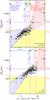 |
Fig. 14 Definition of the various zones for the two models, for R4 (54 pc). Each panel
shows the binned trends of the right panels of Fig. 13 (grey circles with error bars). The fitted trend (black symbols with
error bars) is the grey trend corrected for the offset
|
Figure 14 illustrates this scenario. The two
panels show the binned trends of Fig. 13 with the
starlight intensity, for the two models. The grey circles with error bars show the
original trend, while the black circles with error bars show the trend corrected for the
offset derived
in Table 8. We fit the latter. We decompose the
trends into the three zones described above, by fitting the following function:
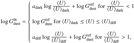 (25)where
adark, adiff,
(25)where
adark, adiff,
 ,
⟨ U ⟩ dark and ⟨ U ⟩ diff
are free parameters. is the
“reference” gas-to-dust mass ratio, i.e. the gas-to-dust mass ratio
in the diffuse ISM, and ⟨ U ⟩ dark and
⟨ U ⟩ diff are the starlight intensities defining these
zones (Fig. 14). Table 9 gives the main parameters of these fits for each model.
,
⟨ U ⟩ dark and ⟨ U ⟩ diff
are free parameters. is the
“reference” gas-to-dust mass ratio, i.e. the gas-to-dust mass ratio
in the diffuse ISM, and ⟨ U ⟩ dark and
⟨ U ⟩ diff are the starlight intensities defining these
zones (Fig. 14). Table 9 gives the main parameters of these fits for each model.
This point of view leads to the same conclusion than in Sect. 4.3.4, namely that the “standard model” is
unphysical. Indeed, the derived reference gas-to-dust mass ratio,
 (Table 9), in regions where dark gas is
unlikely, is on average below the hard limit,
(Table 9), in regions where dark gas is
unlikely, is on average below the hard limit,  . On the contrary, the
“AC model” gives a reference
. On the contrary, the
“AC model” gives a reference  close to the expected value, based on the metallicity of the LMC,
 . More importantly, this
reference ratio does not violate the elemental abundances, with the “AC
model”.
. More importantly, this
reference ratio does not violate the elemental abundances, with the “AC
model”.
In summary, now that we have taken into account the various competing processes, we can safely conclude that the “standard model”, which works for the Milky Way, does not apply to the LMC. It means that the chemical composition of the grains in the LMC is systematically different than that of the Galaxy. The LMC grains have on average a larger submm opacity. Although the possible compositions are numerous, this work gives a plausible one, respecting the elemental abundances, based on optical properties of grains that have been observed in the laboratory (ACAR amorphous carbons in lieu of graphite; Zubko et al. 1996).
4.3.7. Remarks on the submillimiter emissivity index
First, as detailed in Appendix A, our “AC model” has a lower far-IR emissivity index (β ≃ 1.7) than the “standard model” (β = 2). In our case, β does not vary much with wavelength in the Herschel range. However, in general, β is a function of the wavelength, and there are grain species showing strong variations in this range (e.g. Quinten et al. 2002).
Second, the emissivity of our grain model is what we call the intrinsic emissivity. On the other hand, the isothermal fit of an SED with free emissivity index provides the effective emissivity index (noted βeff. by us). The two are similar (β = βeff.) only if the isothermal approximation is valid. On the contrary, if the spatial resolution is such that there is likely a mix of temperatures within the beam, then the two values are going to differ. The SED will be broadened by the temperature distribution and βeff. will likely be lower than β. In the LMC, we are mostly in the second case. Due to this degeneracy, the shapes of the SED do not provide direct constraints on β. Other constraints have to be invoked. In our case, we used the constraints on the gas-to-dust mass ratio to discriminate between different β.
We note that Aguirre et al. (2003), using COBE observations of the LMC, reached the same qualitative conclusion as derived here. They concluded that the grain opacities were different in the LMC than in the Milky Way, although they adopted a different set of grain species. However, these authors based their analysis only on isothermal fits, and did not use the gas-to-dust mass ratio as a constraint. Therefore their demonstration was incomplete. Similarly, Gordon et al. (2010, using Herschel and Planck Collaboration et al. (2011a, using Planck showed that the effective β of the LMC was around 1.5. However, they did not constrain the intrinsic β.
Thus, in light of these precisions, we have shown, for the first time, that the intrinsic far-IR/submm emissivity index of the grains in the LMC is lower than in the Galaxy.
4.3.8. Constraints on the dark gas content
Using the point of view of Fig. 14, we can put an upper limit on the dark gas content. Since we have shown in Sect. 4.3.6 that most of the variation of the gas-to-dust mass ratio could originate in an overlooked gas component, we can estimate the mass of this component, from this point of view.
Properties of the overlooked gas component.
To provide an optimistic estimate, we define the mass of overlooked gas
 by the mass added to the observed gas mass
  ,
in order to match the expected gas-to-dust mass ratio
,
in order to match the expected gas-to-dust mass ratio
 in regions where the uncorrected Gdust is lower than
:
in regions where the uncorrected Gdust is lower than
:
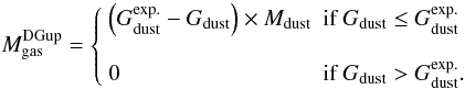 (26)Technically,
this dark gas includes the CO-free H2, as well as a fraction of the
CO-associated H2 where the XCO factor is higher
than our adopted value. This definition implies that this dark component covers most of
the strip with the “standard model”, while it is going to cover only a
fraction of it with the “AC model”. Table 10 gives the mass fraction of this component, for both models, at
each spatial resolution. The most reliable value is probably the value at R4 of the
“AC model”.
(26)Technically,
this dark gas includes the CO-free H2, as well as a fraction of the
CO-associated H2 where the XCO factor is higher
than our adopted value. This definition implies that this dark component covers most of
the strip with the “standard model”, while it is going to cover only a
fraction of it with the “AC model”. Table 10 gives the mass fraction of this component, for both models, at
each spatial resolution. The most reliable value is probably the value at R4 of the
“AC model”.
Therefore, comparing the conservative estimate of Table 8 and the optimistic estimate of Table 10, with their respective uncertainties, we can bracket the dark gas mass
fraction  in the strip, with the
“AC model”.
in the strip, with the
“AC model”.
For comparison, Bernard et al. (2008) found that this fraction was 182%. The reason for this discrepancy might be due to the fact that the region we have modelled here is relatively poor in dark gas, compared to the entire LMC.
4.4. What the SPIRE500 μm excess is not
As mentioned in Sect. 3.3, we have not fitted the SPIRE500 μm excess present in our data. We have excluded this waveband, in order to avoid being biased by this effect, since its origin is still unknown. This excess can, a priori, affect our previous result concerning the grain properties, for two different reasons. First, this excess could originate in colder dust that our model has not accounted for. Our dust mass would then have been biased. Second, if the origin of this excess is an unkown mechanism, not related to cold dust, it could also affect shorter wavelength bands, and bias our dust mass.
Although SPIRE500 μm was not used as a constraint, for our dust SED model, it is possible to study the behaviour of its excess with the physical conditions.
4.4.1. Systematic analysis of the excess
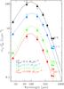 |
Fig. 15 Different SEDs spanning the SPIRE500 μm excess range. These SEDs correspond to four pixels (at resolution R4; 54 pc), arbitrarily chosen. For each pixel the observations (open circle and error bar), the model (AC; solid line), and the model integrated in the broadband filters (filled circle) are displayed. For each SED, the corresponding dust mass surface density and the value of r500 are given. |
Let’s define the absolute and relative excesses of the
SPIRE500 μm band, respectively by: 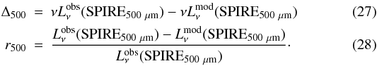 Figure 15 shows four SEDs with different values of the
excess.
Figure 15 shows four SEDs with different values of the
excess.
Absolute and relative SPIRE500 μm excesses as a function of spatial resolution.
Table 11 shows the value of the excesses, as a
function of the spatial resolution. In general, the excess tends to be slightly smaller
with the “AC model”, since it has a slightly flatter submm slope. The
relative excess tends to rise slightly when the spatial resolution decreases, but this
trend is not statistically significant. We emphasize that
r500 being a relative quantity, most of the calibration
error cancels, and the errors quoted in Table 11
are uncorrelated between different spatial resolution. Most of the error in this excess
comes from the noise in the diffuse emission. The most reliable estimates of the excess
are therefore those of R10 (integrated strip):  and
and
 . This excess is only
marginally detected in the global SED. Since, the excess is relatively similar for both
models, and that we have previously shown that the “AC model” is more
realistic, we will discuss the excess only for the “AC model”, in the
rest of this section.
. This excess is only
marginally detected in the global SED. Since, the excess is relatively similar for both
models, and that we have previously shown that the “AC model” is more
realistic, we will discuss the excess only for the “AC model”, in the
rest of this section.
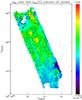 |
Fig. 16 Spatial distributions of the SPIRE500 μm excesses. The spatial resolution is R4 (54 pc). The color image is the absolute excess Δ500, and the contours are the relative excess r500 (the contours are labeled in percent). |
Figure 16 compares the spatial distribution of the absolute SPIRE500 μm excess (Eq. (27), in colors), with the relative excess (Eq. (28), with contours). We first note that the absolute excess is not homogeneous, and contains structures associated with the known features of the LMC, in particular N 44, and the north superbubble. We also note that the absolute value of the excess is much larger than the typical noise (Table 4). We emphasize that the map has been background subtracted in such a way that the fluxes on the north and south of the strip are zero. These arguments show that this excess can not be attributed to emission external to the LMC, like CMB fluctuations or cirrus foreground. The distribution of the relative excess r500 also shows structures, that appear to be roughly anticorrelated with the IR luminosity.
Let’s look in more details at the correlation of the excess with different quantities, in order to decipher its origin. Figure 17 shows the relation of the absolute excess to the gas phases. It shows that the absolute excess is not correlated with the molecular gas, but is correlated with the H i column density. It therefore suggests that the SPIRE500 μm excess is associated with the atomic medium but not with dense phases. To go further, we need to look into the various interpretations that have been proposed, for submm excesses in galaxies.
4.4.2. Consistency test of different interpretations
A submm emission excess has been reported in different systems. We warn the reader that this excess extends up to cm wavelengths. It is still uncertain if the same physical process is responsible for the entire wavelength range, or if it is the combination of several phenomena.
Reach et al. (1995) first reported a long wavelength excess in the COBE/FIRAS spectrum of the Galaxy. This excess could be fit with a very cold dust component (4–7 K). However, the authors rejected this solution, since it was located at high Galactic latitudes. This excess was fit by Li & Draine (2001) invoking a long wavelength enhancement of the opacity of their silicate grains (see also Appendix A). Galliano et al. (2003) discovered a submm excess in the SCUBA and MAMBO observations of the blue compact galaxy NGC1569. Then several studies reporting similar excesses in galaxies, mainly low-metallicity dwarf galaxies were published, e.g.: Dumke et al. (2004), Galliano et al. (2005), Bendo et al. (2006), Galametz et al. (2009, 2010), O’Halloran et al. (2010). The relative intensity of this excess appears to decrease with metallicity (e.g. the sequence SMC, LMC, MW). Planck Collaboration et al. (2011a) presented the global excess at long wavelength.
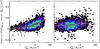 |
Fig. 17 Pixel-to-pixel SPIRE500 μm absolute excess as a function of the column density of the atomic, and detected molecular phase. The spatial resolution is R4, the dust model is “AC”. The color scale is identical to Fig. 13. The error bars correspond to the binned trends. ΣH2 is the column density of molecular gas derived from the CO line observations, but does not account for the dark component detected in Sect. 4.3. The yellow dashed line shows the zero value (no excess). |
The main interpretations of this excess, found in the literature, are the following.
-
1.
Gallianoet al. (2003, 2005)discussed the consequences of a very cold dust component,showing that it was not inconsistent if the emissivity index of thesegrains was β ≃ 1. This scenario would imply a small number (at most a few hundreds) of very dense, parsec-size clumps, containing a large fraction (40−80%) of the ISM mass.
-
2.
Meny et al. (2007) showed that the excess was successfully fit with a physical model of temperature dependent grain emissivity. Their model implies that the emissivity index decreases, when the temperature of the grain increases.
-
3.
Bot et al. (2010) have shown that the long wavelength spectrum of the excess renders the sole very cold hypothesis impossible. It has to be combined with another process to be realistic: e.g. very cold dust and spinning dust grains (Draine & Lazarian 1998). Alternatively, Planck Collaboration et al. (2011a) proposed that the excess in the SMC could be a combination of the Meny et al. (2007) grain model and of spinning grains. However, Planck Collaboration et al. (2011a) attributed the excess in the LMC to CMB fluctuations. Bot et al. (2010) explained the excess in the LMC and SMC with a combination of 12 K dust and spinning grains (Ysard & Verstraete 2010).
Here, we discuss r500 in light of these scenarios.
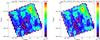 |
Fig. 18 Zoom on N 44 and its surroundings. The color image is
|


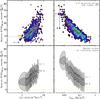 |
Fig. 19 Pixel-to-pixel variations of r500 around N 44, for the “AC model”. This relation includes only the pixels of the window centered around N 44 and displayed in Fig. 18. The spatial resolution is R4. The two top panels show the pixel density number correlations (colors; scale indentical to Fig. 13). The error bars represent the stacked trends in different bins. The central positions and the error bars are the median of the pixel distribution. They account for the scattering of the relation, but not for the error on individual pixels. On the contrary, the two bottom panels show the same trends, but the ellipses are the median error bars on individual pixels (dark: 50%; light: 90%). The excess is significant when looking at resolved scales. The yellow dashed line shows the zero value (no excess). |
Since the actual value of this excess is very sensitive to the noise, let’s zoom into the brightest star forming region of our observations: N 44 and its surroundings. Figure 18 shows the central distribution of the excess around N 44, compared to the starlight intensity and the dust mass column density. Figure 19 shows the corresponding pixel-to-pixel variations. It also demonstrates the typical error bars on individual pixels, showing that the excess is significant when looking at spatially resolved regions. Both ⟨ U ⟩ and Σdust are correlated with r500. However, the correlation is better with Σdust. This is confirmed by the spatial distribution: although, on average the excess corresponds to high starlight intensity regions, there is one spot north of N 44, with no excess and high starlight intensities. Therefore, our observations indicate that the excess is primarily associated with diffuse regions. As a consequence, this excess can not come from contamination by the 12CO(J = 5 → 4)520 μm line.
In regard to these trends, the very cold dust hypothesis is very unlikely. Indeed, we would expect very dense clumps to be associated with dense regions. On the contrary, the observations show that most of these clumps would be present in the diffuse ISM, and very few or none of them in dense regions. However, this is only a qualitative argument showing that very cold dust is unlikely. To rule out this component, we develop the following, more quantitative point of view. In order to reach temperatures below 10 K, very cold dust has to be efficiently shielded. And, the dust responsible for the shielding is going to absorb the ambient radiation and reach warm temperatures, emitting in the wavelength range that has been modelled in the previous sections. We can therefore estimate the mass of shielding dust necessary to allow the very cold dust to reach low temperatures. By comparing the order of magnitude of the minimum mass of shielding dust to the observed mass in each pixel, Appendix D shows that very cold dust can reasonably be ruled out.
Incidentally, by showing: (i) that very cold dust is unlikely to contribute significantly to SPIRE500 μm and (ii) that the SPIRE500 μm excess is found mainly in diffuse regions, we have demonstrated that this excess does not have any impact on our main discussion about dust mass (Sect. 4.3).
5. Summary and conclusion
In this paper, we have presented the modelling of the spatially resolved Spitzer/IRAC, Spitzer/MIPS and Herschel/SPIRE data of a strip covering one quarter of the LMC. The purposes of this work was to:(i) systematically study all the effects leading to inaccuracies or biases affecting the dust mass estimate of a galaxy, in the Herschel era; (ii) explore the peculiar ISM properties of the LMC. Our main results are the following.
-
1.
We have presented an empricial model to fit IR/submm SEDs.This model adopts realistic grain properties, and accounts for apossible distribution of starlight intensity in the region studied.We have described in detail the general propagation of theobservational errors (noise and calibration) through the SEDfitting process. We have shown that, even when thesignal-to-noise ratio is high, the errors on the dust mass areimportant and strongly asymmetric (typically
 ).
However, we have shown that relative quantities (ratio of two parameters) can
have small error bars (typically
).
However, we have shown that relative quantities (ratio of two parameters) can
have small error bars (typically  )
due to the partial cancelation of the correlated calibration errors.
)
due to the partial cancelation of the correlated calibration errors. -
2.
By modelling the same set of maps, but with different pixel sizes, we have shown that the lack of spatial resolution can lead to a systematic underestimate of the dust mass by ≃50%. This bias could be the result of the veiling of cold components by the emission from warmer regions. Although the amplitude of this bias is probably specific to the type of environment found in the LMC and to the wavelength coverage of our data set, we believe that this trend with spatial resolution is general. Modelling the integrated SED of a galaxy leads to underestimating the dust mass.
-
3.
We have performed our SED fitting with two sets of grain composition, in order to explore the sensitivity of the dust mass estimate to the submm emissivity of the grains. We have shown that both compositions give equally good fits, but that the “standard” grain composition (graphite & silicate), that works for the Milky Way, fails to give physically realistic results in the LMC. It violates the elemental abundances. We discuss the fact that this discrepancy could either be due to modified submillimeter grain opacities (our AC model: amorphous carbon & silicate), or to the presence of an unaccounted for gas reservoir. In particular, we have shown that there is a degeneracy between the intrinsic grain emissivity and their temperature distribution, and that considerations on the mass are a powerful way to remove some of this degeneracy.
-
4.
The detailed spatial analysis of the variations of the observed gas-to-dust mass ratio has proven the need for grain opacities different than those of the Galaxy. More precisely, our analysis has demonstrated that grains in the LMC have on average a larger far-IR/submm opacity. We propose a physical dust model that is consistent with these properties (emissivity index β ≃ 1.7, and κabs(160 μm) = 1.6 m2 kg-1), although we insist that this particular composition is not a unique solution.
-
5.
We have shown that the mass averaged starlight intensity is a better tracer of regions where the observed gas-to-dust mass ratio is depleted. Comparing different methods, we have constrained the amount of “dark gas” (i.e. unaccounted for by [H i]21 cm, and 12CO(J = 1 → 0)2.6 mm). This reservoir accounts for ≃ 10–100% of the gas mass of the strip. Simply correcting the standard CO-to-H2 conversion factor is not sufficient to account for this dark gas reservoir, since it is abundant in regions where no CO detection is reported.
-
6.
We have analyzed the excess emission in the SPIRE500 μm waveband, which has been reported before in the LMC and other low-metallicity galaxies. On average the amplitude of the relative excess is ≃15%, and it can vary spatially between 0 and ≃40%. By scrutinizing its behaviour, we show that this excess is mainly anticorrelated with the density of the ISM. We show that this excess can not be due to CMB fluctuations, nor to massive amounts of very cold dust. However, the nature of this excess remains unknown.
Considering the uncertainties in grain optical properties, our study demonstrates that, when modelling the IR/submm SED of a galaxy, the derived dust mass can be considered as a constraint rather than a result. Indeed, we have shown that standard Galactic grain properties were leading to unphysical masses. We therefore have selected another model which was giving reasonable results. However, going from this conclusion to providing the reader with an actual dust mass or gas-to-dust mass ratio for the LMC would be a circular process. It is now clear that grain properties can vary significantly from a galaxy to another. The range of gas-to-dust mass ratios that results from using different grain species makes the estimate of the absolute dust mass irrelevant, without independent constraints. Such independent constraints could be the elemental depletions, or spectroscopic information on the precise chemical composition of the grains, or simultaneous extinction measurements.
Appendix A: The grain properties of our models
A.1. The submillimetre opacities
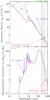 |
Fig. A.1 Comparison of the grain properties of our two models. The top panels show the opacity of the two mixtures. The grey dash lines show long wavelength fits of these opacities, with empirical laws ∝ νβ. The bottom panel compares the SEDs of the two grain mixtures illuminated by the ISRF of the diffuse Galactic ISM (U = 1). |
The top panel of Fig. A.1 compares the
absorption opacities of the grain mixtures of our two models. These opacities are the
sum of PAHs, carbon grains and silicates. The effective submillimeter emissivity index
β is defined by the logarithmic index of the opacity: 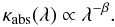 (A.1)It is
β ≃ 2 for the “standard model” and
β ≃ 1.7 for the “AC model”, although
β for amorphous carbons alone is even lower. Table A.1 gives the submilimeter properties of our two
models approximated by Eq. (A.1).
(A.1)It is
β ≃ 2 for the “standard model” and
β ≃ 1.7 for the “AC model”, although
β for amorphous carbons alone is even lower. Table A.1 gives the submilimeter properties of our two
models approximated by Eq. (A.1).
Submillimeter properties of our dust compositions.
The bottom panel compares the infrared emission of the compositions, for the same starlight intensity. It demonstrates that the “AC model” has more emissivity, especially in the submm. It therefore allows us to fit the same observed SED with less mass, and slightly hotter grains.
Fitting the COBE/FIRAS high latitude Galactic cirrus, Li & Draine (2001) had to modify the imaginary part of the dielectric function of their silicate grains, at wavelengths greater than 250 μm. This modification would have a very limited effect on our conclusion, since our constraints go up to 350 μm only, where this increase is very limited (it is ± 12% in the 250 μm ≤ λ ≤ 1000 μm range). This modification actually lowers the emissivity between 250 and 850 μm, and increases it, at λ > 850 μm. For our dust mixture, the amplitude of this modification is even lower, since the contribution of silicates to the far-IR is lower than for the Li & Draine (2001) model. The difference between the “standard model” and the one using the modified silicate of Li & Draine (2001) is invisible in Fig. A.1. The physical origin of this excess may be similar to the one we find here. However, its amplitude is much larger in the LMC, and manifests at shorter wavelengths (λ ≳ 100 μm).
A.2. Size distribution considerations
It is important to note that the size distribution used here does not include grains larger than 0.35 μm, and the contribution to the emission of grains larger than a ≳ 0.1 μm is negligible. Large grains tend to have a flat UV-visible opacity, and therefore, to have a lower equilibrium temperature than smaller equilibrum grains, exposed to the same ISRF. Therefore, adding larger grains would increase the submillimetre emissivity of the model, and allow us to fit the SPIRE fluxes, without having to go to low starlight intensities. However, having large grains or having colder dust would give the same discrepancies in terms of gas-to-dust mass ratios. Moreover, a significant excess of large grains would flatten the UV rise of the extinction curve, contradicting the observations of several lines of sight within the LMC (Gordon et al. 2003).
Another feature of our model is that we have been forced to lower the abundance of non-PAH small grains (a < 10 nm; both carbon and silicate grains) by a factor of 2. Without this modification, we were not able to get good fits of the MIPS24 μm of the diffuse regions. This modification has a very minor effect on the dust mass (≲ 10%), and it is systematic, thus it has no impact on our conclusions. However, this is puzzling since the fit of the extinction curves of the LMC indicates a larger fraction of small grains (e.g. Weingartner & Draine 2001). The fact is that the Zubko et al. (2004, BARE-GR-S) model has a higher small grain contribution in MIPS24 μm than the Draine & Li (2007). On the other hand, replacing graphite by amorphous carbon, as shown in this paper, allows us to get rid of the 30 μm graphite feature, and decrease the contribution of small grains in the MIPS24 μm band, making the 24 μm fit better without having to alter the size distribution. This is another indirect consistency check of the conclusion of this paper.
A.3. Overview of the derived PAH properties
Although the scope of our paper was not to discuss the PAH properties, their abundance is a natural output of our model. In this section, we summarize these results.
PAH mass fraction as a function of spatial resolution.
Table A.2 shows the PAH mass fractions for the two models. This parameter is relatively well constrained and does not vary significantly with spatial resolution. Indeed, it depends essentially on the IRAC8 μm-to-total-IR luminosity ratio. The mass fraction for the “AC model” is systematically higher, since the bulk of the dust is more emissive.
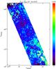 |
Fig. A.2 PAH mass fraction, fPAH. The map is shown for the “AC model”, at spatial resolution R1 (54 pc). |
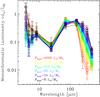 |
Fig. B.1 Classes of observed SEDs for the “standard model”. The SEDs
are normalised by their integrated IR luminosity,
LIR. The classes are ordered according to their
specific power |

Figure A.2 shows the spatial distribution of the mass fraction of PAHs, fPAH (Eq. (3)). We confirm the Paradis et al. (2009) results showing an excess of PAH emission toward the stellar bar. However, fPAH is biased by the fact that, in absence of detailed mid-IR spectrum, we have arbitrarily fixed the charge fraction to 1/2. The charge fraction controls the emissivity of the C-C modes (Galliano et al. 2008b). Therefore, it is difficult to uniquely interpret this excess emissivity by a local increase of the PAH abundance.
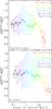 |
Fig. B.2 Bias in the dust mass estimate as a function of the starlight intensity, for
both models. In each panel, we plot the ratio of the median of the dust masses
measured by fitting the randomly perturbed SEDs of Fig. B.1 ( |
Appendix B: Details concerning the error analysis
B.1. Classes of observed SEDs
The error analysis presented in Sect. 3.4 would imply having to fit the 156 577 pixels (Table 1) 300 times with the two models, leading to a total of ≃108 fits. However, all these SEDs have a lot of similarities, and it is not necessary to perform the Monte Carlo iterations on each pixels. Here we describe the approximation method we demonstrated in Fig. 4.
We start from the actual fit of the unperturbed SED of each pixel of Table 1. We order these SEDs according to their specific
emitted power  ,
making 30 logarithmic bins. Figure B.1 shows the
classes of observed SEDs, for the “standard model”. At each waveband
λ0, the central value is the median of the normalized
monochromatic power
λ0Lλ0/LIR
of each pixel within the considered bin of specific power. The error shows the
dispersion of the pixels within the bin. On first approximation, the specific power is
proportional to the mass averaged starlight intensity ⟨ U ⟩ . That
is the reason why the SEDs of Fig. B.1 are
nicely ordered according to the wavelength peak of the dust emission. Notice that the
dispersion at most wavebands is small compared to the variation spread by the
different classes. The only wavelength range where it is not true is the near-IR
(λ ≲ 5 μm), where the stellar emission dominates.
,
making 30 logarithmic bins. Figure B.1 shows the
classes of observed SEDs, for the “standard model”. At each waveband
λ0, the central value is the median of the normalized
monochromatic power
λ0Lλ0/LIR
of each pixel within the considered bin of specific power. The error shows the
dispersion of the pixels within the bin. On first approximation, the specific power is
proportional to the mass averaged starlight intensity ⟨ U ⟩ . That
is the reason why the SEDs of Fig. B.1 are
nicely ordered according to the wavelength peak of the dust emission. Notice that the
dispersion at most wavebands is small compared to the variation spread by the
different classes. The only wavelength range where it is not true is the near-IR
(λ ≲ 5 μm), where the stellar emission dominates.
B.2. Class interpolation and error estimate
We perform the Monte Carlo error analysis of Sect. 3.4.2 on each SED class, for 6 different noise levels, spanning the whole
range of observed signal-to-noise ratios, S/N. We perform this study with the two
models. Then, for each pixel of Table 1, the
errors on the parameters are determined by logarithmically interpolating the
precomputed errors in  and S/N.
The validity of this interpolation method is demonstrated in Fig. 4. We show that this method reproduces well the central value and error bars of each parameter, since it reproduces well the skewness of the probability distribution.
B.3. Biases of the SED fits
The large database of Monte-Carlo fits of the SEDs of Fig. B.1 can be used to study the systematic effects of our method. Figure B.2 shows the bias on the dust mass, as a function of the mean equilibrium grain temperature.
The two panels of this figure correspond to the two models. The
x-axis is the “actual” ⟨ U ⟩ ,
i.e. the value of ⟨ U ⟩ derived from the unperturbed SEDs of
Fig. B.1. Each value of
⟨ U ⟩ defines one of the 30 classes, since
 .
The y-axes show the ratio between:
.
The y-axes show the ratio between:
 ,
which is the median of the mass estimates derived from the fitting of the 300
Monte-Carlo perturbed SEDs of each class; and
,
which is the median of the mass estimates derived from the fitting of the 300
Monte-Carlo perturbed SEDs of each class; and  which is
the dust mass corresponding to the unperturbed SED. In other words,
which is
the dust mass corresponding to the unperturbed SED. In other words,
 quantifies the deviation from the dust mass derived from an SED fit, to its actual
value, as a function of the starlight intensity.
quantifies the deviation from the dust mass derived from an SED fit, to its actual
value, as a function of the starlight intensity.
Figure B.2 shows that up to ⟨ U ⟩ Std ≲ 6 and ⟨ U ⟩ AC ≲ 9, the dust masses derived from SED fits are not significantly biased (i.e. the deviation is smaller than the error bars). However, for starlight intensities higher than these values, the SED fit tends to systematically underestimate the dust masses (i.e. overestimate the gas-to-dust mass ratio). The amplitude of this effect can go up to a factor of ≃2, for high ⟨ U ⟩ .
This is a demonstration of the effect invoked to explain the low gas-to-dust mass ratio, at high starlight intensities, in Fig. 14. Fortunately, this effect concerns only a regime containing a small fraction of the pixels. Moreover, these pixels are the less massive, since they correspond to hot and diffuse regions. Therefore, this bias does not have a significant impact on our global dust mass estimate.
Appendix C: Relevance of our starlight intensity distribution
C.1. The unnecessariness of adding a diffuse field component
We note that our approach of modelling IR SEDs with an empirical combination of
starlight intensities, is common in the literature. In particular, Draine et al. (2007) modelled the SEDs of the SINGS
galaxies with an extra, uniformly illuminated, component: 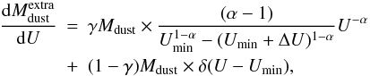 (C.1)where
γ is an extra parameter controlling the mass fraction of the
U−α component. This formulation
implicitly assumes that there are no massive quantities of dust colder than the
diffuse ISM. One of the advantages of this extra component is to avoid the dust mass
to diverge, in the absence of submm constraints. Indeed, as demonstrated by Galametz et al. (2011), modelling the SEDs of
galaxies without submm data, using Eq. (4), leads to gross errors on the dust mass. However, in our case, we have
the valuable submm constraints provided by Herschel. The relevance of
this extra component can be tested using the Monte-Carlo method, described in
Sect. 3.4.2.
(C.1)where
γ is an extra parameter controlling the mass fraction of the
U−α component. This formulation
implicitly assumes that there are no massive quantities of dust colder than the
diffuse ISM. One of the advantages of this extra component is to avoid the dust mass
to diverge, in the absence of submm constraints. Indeed, as demonstrated by Galametz et al. (2011), modelling the SEDs of
galaxies without submm data, using Eq. (4), leads to gross errors on the dust mass. However, in our case, we have
the valuable submm constraints provided by Herschel. The relevance of
this extra component can be tested using the Monte-Carlo method, described in
Sect. 3.4.2.
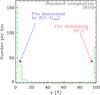 |
Fig. C.1 Test of the stability of the starlight intensity distribution of Eq. (C.1). The parameter γ is the mass fraction of the component in U−α. The histogram is the distribution of the Monte-Carlo iterations of the fit of Eq. (C.1) to the integrated strip (R10), with the grain composition of the “standard model”. The bimodality of the distribution is the sign of the instability of this formalism. |
First, we tested the stability of this extra component. Figure C.1 shows the distribution of the Monte-Carlo values of γ, when fitting the integrated SED strip (R10), with Eq. (C.1) and the “standard” grain composition. This distribution is drastically bimodal. Most of the perturbed SEDs are fit either without the extra δ(U − Umin) components (γ ≃ 1) – which is equivalent to our model – or with a sole uniformly illuminated SED (γ ≃ 0). In other words, the value of the parameter γ is totally uncertain.
Second, we tested the statistical relevance of adding this extra component. To
quantify this aspect, we performed a F-test. We computed the statistic
Fχ (Bevington & Robinson 2003):
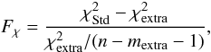 (C.2)where
 is the
χ2 (Eq. (8)) of the fit of a given perturbed SED of the integrated strip with the
“standard model”, and
is the
χ2 (Eq. (8)) of the fit of a given perturbed SED of the integrated strip with the
“standard model”, and  is the
corresponding value for Eq. (C.1);
n = 10 is the number of wavebands, and
mextra = 7 is the number of free parameters for the
model of Eq. (C.1) plus the stellar
component of Eq. (7).
Fχ can be seen as a measure of how much
the additional term has improved the value of the reduced
χ2. Statistically,
is the
corresponding value for Eq. (C.1);
n = 10 is the number of wavebands, and
mextra = 7 is the number of free parameters for the
model of Eq. (C.1) plus the stellar
component of Eq. (7).
Fχ can be seen as a measure of how much
the additional term has improved the value of the reduced
χ2. Statistically,
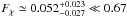 is lower than the value
of the F-distribution, with
n − mextra − 1 = 2 degrees of freedom,
with a probability of exceeding Fχ of 50%
(or
PF(0.67,1,n − mextra − 1) = 50%;
Bevington & Robinson 2003). In other
words, adding the extra component of Eq. (C.1) does not significantly improve the χ2. Our
starlight intensity distribution (Eq. (4)) is therefore statistically more significant.
is lower than the value
of the F-distribution, with
n − mextra − 1 = 2 degrees of freedom,
with a probability of exceeding Fχ of 50%
(or
PF(0.67,1,n − mextra − 1) = 50%;
Bevington & Robinson 2003). In other
words, adding the extra component of Eq. (C.1) does not significantly improve the χ2. Our
starlight intensity distribution (Eq. (4)) is therefore statistically more significant.
Finally, we tested the conservativeness of the dust mass estimate with Eq. (C.1). We have performed the fits of
exactly the same perturbed SEDs that were used in Fig. C.1, with our “standard model” (Eq. (4)). The ratio of the mass of our model to
the mass obtained with the extra component is 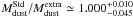 .
In other words, the two starlight intensity distributions of Eqs. (4) and (C.1) give statistically identical dust masses, within a few
percents.
.
In other words, the two starlight intensity distributions of Eqs. (4) and (C.1) give statistically identical dust masses, within a few
percents.
In summary, for the analysis performed in this paper, the starlight intensity distribution of Eq. (C.1) is not physically motivated, neither statistically stable nor relevant, and gives identical results to Eq. (4). Our model has an appropriate balance between free parameters and observational constraints. It is flexible enough, but it does not lead to overinterpreting the data.
C.2. Comparison of our model with the isothermal approximation
As justified in Sect. 3, our model accounts for a distribution of equilibrium dust temperatures within each pixel (Eq. (4)). This formalism allows us to fit the submm slope more accurately than with a single temperature. As a consequence, our model predicts more mass than a single black body fit having the same dust opacity. Since the single black body approach is still widely used, even in the Herschel era, we have performed a systematic comparison in order to quantify the biases of such an approach.
To perform our comparison, we have fitted the R4 (54 pc) map with a single modified
black body having the same grain opacity as our “standard model”:
κabs(160 μm) = 1.4m2 kg-1,
and β = 2 (Fig. A.1). For each
pixel, the mass and the temperature are free to vary, but β is kept
fixed. We constrain this model with the MIPS70 μm,
MIPS160 μm, SPIRE250 μm
and SPIRE500 μm fluxes, weighted the same way as our
complete model (Eq. (8)), except that
the weight of the MIPS70 μm flux is divided by 100. The
purpose of this trick is the following: (i) when the peak of the SED
is well constrained by MIPS160 μm,
SPIRE250 μm and
SPIRE350 μm (low temperatures), the
MIPS70 μm flux has almost no impact on the
χ2; (ii) when the peak is not well
constrained (high temperatures), the MIPS70 μm becomes
important and temperature divergence is avoided. The mass for each pixel is noted
 .
.
 |
Fig. C.2 Comparison between our standard model and a single black body
fit. The spatial resolution is R4 (54 pc). The x axis is the
mass starlight averaged intensity ⟨ U ⟩ of the
“standard model”. The y axis is the ratio
between the dust derived with a single black body fit
|


Figure C.2 shows the ratio between the dust masses obtained with this isothermal fit and with our “standard model”, as a function of the mass averaged starlight intensity ⟨ U ⟩ . It shows that for ⟨ U ⟩ ≳ 1, the mass ratio is roughly constant between 60 and 80%, but for ⟨ U ⟩ ≲ 1, the ratio drops down to less than 30%. This simulation demonstrates that an isothermal fit will induce a bias in dust masses with average temperature. The regions with high starlight intensities (⟨ U ⟩ ≳ 1) are generally diffuse regions and their SEDs are almost isothermal. This explains why the mass ratio does not vary much with starlight intensity in this range. The average value of the ratio is around 70% in these regions, which is reasonable considering the crudeness of the approximation. On the contrary, regions with low starlight intensities (⟨ U ⟩ ≲ 1) are generally dense regions. Since the mean free path of photons is much shorter in these regions, there is a significant mix of cold and hot components within each pixel. The isothermal approximation is not valid anymore in this range of ⟨ U ⟩ , and the mass obtained with a single black body fit is biased. Namely, it drops by a factor of ≃2 compared to its diffuse ISM value, down to ≃30% of the value of the “standard model”. We obtain a similar trend comparing the “AC model” with a single black body fit having κabs(160 μm) = 1.6m2 kg-1, and β = 1.7, except that the values of ⟨ U ⟩ are systematically shifted by a factor of ≃2 (as demonstrated in Fig. 5).
Finally, we note that the increase of dust mass at low starlight intensities compared to the isothermal approximation is unlikely a bias induced by the submm excess extending down to the SPIRE350 μm band. Indeed, this excess is negligible in regions with low ⟨ U ⟩ (Sect. 4.4). It is prominent only in regions with high ⟨ U ⟩ , where the trend of Fig. C.2 is not significant.
Appendix D: Inconsistency of the very cold dust hypothesis
As discussed by Galliano et al. (2003, 2005) and Galametz
et al. (2009, 2010), the
SPIRE500 μm excess could be attributed to very cold dust
(VCD;  ). Simply considering the shape
of the SED, this explanation is not unlikely. Such a component would produce a change in
the submm slope of the SED. Indeed, warm and cold dust are heated by the transmitted
stellar light, in different environments, at different optical depths. Their temperature
distribution is therefore continuous. On the other hand, in order to reach very
cold temperatures (Tdust ≲ 10K), the dust has to be
fully shielded from stellar radiation. In these conditions, the dominant heating sources
are the collisions and the IR radiation (galaxy and CMB) which do not depend on the
optical depth. It could reach temperatures lower than
Tdust ≃ 5K (Galliano et al.
2003) only with difficulty. Very cold dust therefore corresponds to a change of
regime in the dust heating. If it exists, its temperature should not significantly vary
with the optical depth in the cloud. Consequently its emission would be seen as a
roughly isothermal component at 5K ≲ Tdust ≲ 10K. With
sufficient mass, it would produce an excess emission, with a change of slope, at
wavelengths 300 μm ≲ λ ≲ 1mm.
). Simply considering the shape
of the SED, this explanation is not unlikely. Such a component would produce a change in
the submm slope of the SED. Indeed, warm and cold dust are heated by the transmitted
stellar light, in different environments, at different optical depths. Their temperature
distribution is therefore continuous. On the other hand, in order to reach very
cold temperatures (Tdust ≲ 10K), the dust has to be
fully shielded from stellar radiation. In these conditions, the dominant heating sources
are the collisions and the IR radiation (galaxy and CMB) which do not depend on the
optical depth. It could reach temperatures lower than
Tdust ≃ 5K (Galliano et al.
2003) only with difficulty. Very cold dust therefore corresponds to a change of
regime in the dust heating. If it exists, its temperature should not significantly vary
with the optical depth in the cloud. Consequently its emission would be seen as a
roughly isothermal component at 5K ≲ Tdust ≲ 10K. With
sufficient mass, it would produce an excess emission, with a change of slope, at
wavelengths 300 μm ≲ λ ≲ 1mm.
Until now, we did not have the spatial resolution to explore this hypothesis. In this section, we do an order of magnitude estimate to test the likeliness of the VCD model. What follows is an update of the discussion at the end of Galliano et al. (2003). This is a complement to Sect. 4.4.2.
Let’s first assume that the excess originates in equilibrium grains having the UV-to-IR
cross-section of silicates: 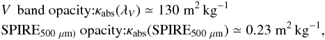 (D.1)and
a submillimeter opacity index βVCD = 1, and an equilibrium
temperature of
(D.1)and
a submillimeter opacity index βVCD = 1, and an equilibrium
temperature of  K.
Those are the most optimistic values. If we can invalidate them, then the VCD hypothesis
will be unrealistic for lower temperatures, steeper submm opacities, and larger UV
cross-sections.
K.
Those are the most optimistic values. If we can invalidate them, then the VCD hypothesis
will be unrealistic for lower temperatures, steeper submm opacities, and larger UV
cross-sections.
Although the relative excess is stronger in diffuse regions, we find an excess in
almost every pixel of the strip (Fig. 16). Let’s
assume that VCD lies in the core of very dense spherical clumps in the diffuse ISM.
Then, the ISRF they have to be shielded from is the typical ISRF of the diffuse ISM. For
the more realistic model (“AC”), this is basically
⟨ U ⟩ ≳ 3. The optical depth, assuming a slab extinction, to shield
this dust, and to allow it to reach  is
is
 .
Since these clumps have to be small, and that we see the excess everywhere, it means
that each clump is unresolved, even at R1. Therefore, the diameter of these clumps has
to be lower than the pixel size of R1, which is
lpix(R1) ≃ 10 pc.
.
Since these clumps have to be small, and that we see the excess everywhere, it means
that each clump is unresolved, even at R1. Therefore, the diameter of these clumps has
to be lower than the pixel size of R1, which is
lpix(R1) ≃ 10 pc.
This maximum size translates into a minimum density of
 , in order
to reach the required optical depth of :
, in order
to reach the required optical depth of :
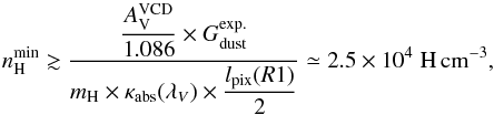 (D.2)mHbeing
the mass of an H atom. Notice that, since we are performing only an order of magnitude
estimate, we use the slab extinction for a sphere.
(D.2)mHbeing
the mass of an H atom. Notice that, since we are performing only an order of magnitude
estimate, we use the slab extinction for a sphere.
With ⟨ U ⟩ ≃ 3, the temperature of the shielding dust, around the
core, is  . Thus, a typical excess of
r500 ≃ 15% corresponds to a mass ratio, between the VCD
core and the shielding ISM dust around, of:
. Thus, a typical excess of
r500 ≃ 15% corresponds to a mass ratio, between the VCD
core and the shielding ISM dust around, of:
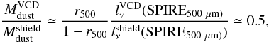 (D.3)lνbeing
the specific monochromatic power of the components. Therefore, for this picture to be
correct, there should be at least
(D.3)lνbeing
the specific monochromatic power of the components. Therefore, for this picture to be
correct, there should be at least  of shielding
ISM dust surface density, such that:
of shielding
ISM dust surface density, such that:
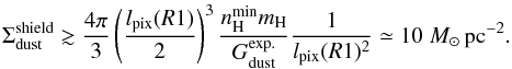 (D.4)This value is 2
orders of magnitude higher than the typical dust mass surface density, and one order of
magnitude higher than the highest values (Fig. 13). Moreover, this argument is conservative, since the highest excesses are
found in lowest surface density regions (Sect. 4.4).
(D.4)This value is 2
orders of magnitude higher than the typical dust mass surface density, and one order of
magnitude higher than the highest values (Fig. 13). Moreover, this argument is conservative, since the highest excesses are
found in lowest surface density regions (Sect. 4.4).
In summary, we have shown that the SPIRE500 μm excess could not be accounted for by very cold dust, since it would require a minimum mass of shielding dust, within each pixel, too large compared to the observed surface density. It is equivalent to note that, the excess being present in most pixels of R1, we would need at least 105 clumps of cold dust. It is more efficient to hide very cold dust in a small number of clumps. For example, Galliano et al. (2003) estimated that this number could be less than a few hundreds in the Magellanic dwarf galaxy NGC1569.
In this paper, we choose the “dark gas” terminology, to remain more general. However, we acknowledge that CO-free molecular gas is not dark, since its dust grains are radiating and it likely emits copious amounts of [Cii].
Acknowledgments
We would like to thank Anthony Jones, Vincent Guillet, Laurent Verstraete, Bruce Draine and Karl Gordon for stimulating discussions on the matter of this paper. We thank the anonymous referee, for his report, and the editor, Malcolm Walmsley, for his careful reading of the paper. We acknowledge extensive use of the Levenberg-Marquardt χ2 minimization routine written by Craig Markwardt. SPIRE has been developed by a consortium of institutes led by Cardiff Univ. (UK) and including Univ. Lethbridge (Canada); NAOC (China); CEA, LAM (France); IFSI, Univ. Padua (Italy); IAC (Spain); Stockholm Observatory (Sweden); Imperial College London, RAL, UCL-MSSL, UKATC, Univ. Sussex (UK); Caltech, JPL, NHSC, Univ. Colorado (USA). This development has been supported by national funding agencies: CSA (Canada); NAOC (China); CEA, CNES, CNRS (France); ASI (Italy); MCINN (Spain); SNSB (Sweden); STFC, UKSA (UK); and NASA (USA).
References
- Aguirre, J. E., Bezaire, J. J., Cheng, E. S., et al. 2003, ApJ, 596, 273 [NASA ADS] [CrossRef] [Google Scholar]
- Bendo, G. J., Buckalew, B. A., Dale, D. A., et al. 2006, ApJ, 645, 134 [NASA ADS] [CrossRef] [Google Scholar]
- Bernard, J.-P., Reach, W. T., Paradis, D., et al. 2008, AJ, 136, 919 [NASA ADS] [CrossRef] [Google Scholar]
- Berné, O., Joblin, C., Deville, Y., et al. 2007, A&A, 469, 575 [NASA ADS] [CrossRef] [EDP Sciences] [Google Scholar]
- Bevington, P. R., & Robinson, D. K. 2003, Data reduction and error analysis for the physical sciences, 3rd ed. (Boston, MA: McGraw-Hill) [Google Scholar]
- Bot, C., Ysard, N., Paradis, D., et al. 2010, A&A, 523, A20 [NASA ADS] [CrossRef] [EDP Sciences] [Google Scholar]
- Compiègne, M., Verstraete, L., Jones, A., et al. 2011, A&A, 525, A103 [NASA ADS] [CrossRef] [EDP Sciences] [Google Scholar]
- Cormier, D., Madden, S. C., Hony, S., et al. 2010, A&A, 518, L57 [NASA ADS] [CrossRef] [EDP Sciences] [Google Scholar]
- Dale, D. A., Helou, G., Contursi, A., Silbermann, N. A., & Kolhatkar, S. 2001, ApJ, 549, 215 [NASA ADS] [CrossRef] [Google Scholar]
- Draine, B. T. 2003a, ARA&A, 41, 241 [NASA ADS] [CrossRef] [Google Scholar]
- Draine, B. T. 2003b, ApJ, 598, 1017 [NASA ADS] [CrossRef] [Google Scholar]
- Draine, B. T. 2009, in ASP Conf. Ser. 414, ed. T. Henning, E. Grün, & J. Steinacker, 453 [Google Scholar]
- Draine, B. T., & Anderson, N. 1985, ApJ, 292, 494 [NASA ADS] [CrossRef] [Google Scholar]
- Draine, B. T., & Lazarian, A. 1998, ApJ, 508, 157 [NASA ADS] [CrossRef] [Google Scholar]
- Draine, B. T., & Li, A. 2007, ApJ, 657, 810 [NASA ADS] [CrossRef] [Google Scholar]
- Draine, B. T., Dale, D. A., Bendo, G., et al. 2007, ApJ, 663, 866 [NASA ADS] [CrossRef] [Google Scholar]
- Dumke, M., Krause, M., & Wielebinski, R. 2004, A&A, 414, 475 [NASA ADS] [CrossRef] [EDP Sciences] [Google Scholar]
- Dwek, E., Arendt, R. G., Fixsen, D. J., et al. 1997, ApJ, 475, 565 [NASA ADS] [CrossRef] [Google Scholar]
- Engelbracht, C. W., Blaylock, M., Su, K. Y. L., et al. 2007, PASP, 119, 994 [NASA ADS] [CrossRef] [Google Scholar]
- Engelbracht, C. W., Rieke, G. H., Gordon, K. D., et al. 2008, ApJ, 678, 804 [NASA ADS] [CrossRef] [Google Scholar]
- Fioc, M., & Rocca-Volmerange, B. 1997, A&A, 326, 950 [NASA ADS] [Google Scholar]
- Fitzpatrick, E. L., & Massa, D. 2005, AJ, 130, 1127 [NASA ADS] [CrossRef] [Google Scholar]
- Fukui, Y., Kawamura, A., Minamidani, T., et al. 2008, ApJS, 178, 56 [NASA ADS] [CrossRef] [Google Scholar]
- Galametz, M., Madden, S., Galliano, F., et al. 2009, A&A, 508, 645 [NASA ADS] [CrossRef] [EDP Sciences] [Google Scholar]
- Galametz, M., Madden, S. C., Galliano, F., et al. 2010, A&A, 518, L55 [NASA ADS] [CrossRef] [EDP Sciences] [Google Scholar]
- Galametz, M., Madden, S. C., Galliano, F., et al. 2011, A&A, 532, A56 [NASA ADS] [CrossRef] [EDP Sciences] [Google Scholar]
- Galliano, F., Madden, S. C., Jones, A. P., et al. 2003, A&A, 407, 159 [NASA ADS] [CrossRef] [EDP Sciences] [Google Scholar]
- Galliano, F., Madden, S. C., Jones, A. P., Wilson, C. D., & Bernard, J.-P. 2005, A&A, 434, 867 [NASA ADS] [CrossRef] [EDP Sciences] [Google Scholar]
- Galliano, F., Dwek, E., & Chanial, P. 2008a, ApJ, 672, 214 [NASA ADS] [CrossRef] [Google Scholar]
- Galliano, F., Madden, S. C., Tielens, A. G. G. M., Peeters, E., & Jones, A. P. 2008b, ApJ, 679, 310 [NASA ADS] [CrossRef] [Google Scholar]
- Gordon, K. D., Clayton, G. C., Misselt, K. A., Landolt, A. U., & Wolff, M. J. 2003, ApJ, 594, 279 [NASA ADS] [CrossRef] [EDP Sciences] [Google Scholar]
- Gordon, K. D., Engelbracht, C. W., Fadda, D., et al. 2007, PASP, 119, 1019 [NASA ADS] [CrossRef] [Google Scholar]
- Gordon, K. D., Galliano, F., Hony, S., et al. 2010, A&A, 518, L89 [NASA ADS] [CrossRef] [EDP Sciences] [Google Scholar]
- Grevesse, N., & Sauval, A. J. 1998, Space Sci. Rev., 85, 161 [NASA ADS] [CrossRef] [Google Scholar]
- Grossi, M., Hunt, L. K., Madden, S., et al. 2010, A&A, 518, L52 [NASA ADS] [CrossRef] [EDP Sciences] [Google Scholar]
- Guhathakurta, P., & Draine, B. T. 1989, ApJ, 345, 230 [NASA ADS] [CrossRef] [Google Scholar]
- Hallenbeck, S. L., Nuth, III, J. A., & Nelson, R. N. 2000, ApJ, 535, 247 [NASA ADS] [CrossRef] [Google Scholar]
- Hony, S., Galliano, F., Madden, S. C., et al. 2010, A&A, 518, L76 [NASA ADS] [CrossRef] [EDP Sciences] [Google Scholar]
- Israel, F. P. 1997, A&A, 328, 471 [NASA ADS] [Google Scholar]
- Israel, F. P., Wall, W. F., Raban, D., et al. 2010, A&A, 519, A67 [NASA ADS] [CrossRef] [EDP Sciences] [Google Scholar]
- Jones, A. P. 2004, in Astrophysics of Dust, ed. A. N. Witt, G. C. Clayton, & B. T. Draine, ASP Conf. Ser., 309, 347 [Google Scholar]
- Jones, A. P., Tielens, A. G. G. M., & Hollenbach, D. J. 1996, ApJ, 469, 740 [NASA ADS] [CrossRef] [Google Scholar]
- Kemper, F., Woods, P. M., Antoniou, V., et al. 2010, PASP, 122, 683 [NASA ADS] [CrossRef] [Google Scholar]
- Kim, S., Staveley-Smith, L., Dopita, M. A., et al. 2003, ApJS, 148, 473 [NASA ADS] [CrossRef] [Google Scholar]
- Laor, A., & Draine, B. T. 1993, ApJ, 402, 441 [NASA ADS] [CrossRef] [Google Scholar]
- Leroy, A., Bolatto, A., Stanimirovic, S., et al. 2007, ApJ, 658, 1027 [NASA ADS] [CrossRef] [Google Scholar]
- Leroy, A. K., Bolatto, A., Bot, C., et al. 2009, ApJ, 702, 352 [NASA ADS] [CrossRef] [Google Scholar]
- Leroy, A. K., Bolatto, A., Gordon, K., et al. 2011, ArXiv e-prints [Google Scholar]
- Li, A., & Draine, B. T. 2001, ApJ, 554, 778 [Google Scholar]
- Lisenfeld, U., & Ferrara, A. 1998, ApJ, 496, 145 [NASA ADS] [CrossRef] [Google Scholar]
- Madden, S. C. 2000, New Astron. Rev., 44, 249 [NASA ADS] [CrossRef] [Google Scholar]
- Madden, S. C., Poglitsch, A., Geis, N., Stacey, G. J., & Townes, C. H. 1997, ApJ, 483, 200 [NASA ADS] [CrossRef] [MathSciNet] [Google Scholar]
- Madden, S. C., Galliano, F., Jones, A. P., & Sauvage, M. 2006, A&A, 446, 877 [NASA ADS] [CrossRef] [EDP Sciences] [Google Scholar]
- Madden, S. C., Galametz, M., Cormier, D., et al. 2011 [arXiv:1105.1006] [Google Scholar]
- Mathis, J. S., Mezger, P. G., & Panagia, N. 1983, A&A, 128, 212 [NASA ADS] [Google Scholar]
- Meixner, M., Gordon, K. D., Indebetouw, R., et al. 2006, AJ, 132, 2268 [NASA ADS] [CrossRef] [Google Scholar]
- Meixner, M., Galliano, F., Hony, S., et al. 2010, A&A, 518, L71 [NASA ADS] [CrossRef] [EDP Sciences] [Google Scholar]
- Meny, C., Gromov, V., Boudet, N., et al. 2007, A&A, 468, 171 [Google Scholar]
- O’Halloran, B., Galametz, M., Madden, S. C., et al. 2010, A&A, 518, L58 [NASA ADS] [CrossRef] [EDP Sciences] [Google Scholar]
- Pagel, B. E. J. 2003, in ASP Conf. Ser. 304, ed. C. Charbonnel, D. Schaerer, & G. Meynet, 187 [Google Scholar]
- Paradis, D., Reach, W. T., Bernard, J., et al. 2009, AJ, 138, 196 [NASA ADS] [CrossRef] [Google Scholar]
- Peeters, E., Martín-Hernández, N. L., Damour, F., et al. 2002, A&A, 381, 571 [NASA ADS] [CrossRef] [EDP Sciences] [Google Scholar]
- Planck Collaboration, Ade, P. A. R., Aghanim, N., et al. 2011a, A&A, 536, A17 [NASA ADS] [CrossRef] [EDP Sciences] [Google Scholar]
- Planck Collaboration, Ade, P. A. R., Aghanim, N., et al. 2011b, A&A, 536, A19 [NASA ADS] [CrossRef] [EDP Sciences] [Google Scholar]
- Poglitsch, A., Krabbe, A., Madden, S. C., et al. 1995, ApJ, 454, 293 [NASA ADS] [CrossRef] [Google Scholar]
- Poteet, C. A., Megeath, S. T., Watson, D. M., et al. 2011, ApJ, 733, L32 [NASA ADS] [CrossRef] [Google Scholar]
- Press, W. H., Teukolsky, S. A., Vetterling, W. T., & Flannery, B. P. 1992, Numerical recipes in FORTRAN, The art of scientific computing, ed. W. H. Press, S. A. Teukolsky, W. T. Vetterling, & B. P. Flannery [Google Scholar]
- Quinten, M., Kreibig, U., Henning, T., & Mutschke, H. 2002, Appl. Opt., 41, 7102 [NASA ADS] [CrossRef] [Google Scholar]
- Reach, W. T., Dwek, E., Fixsen, D. J., et al. 1995, ApJ, 451, 188 [NASA ADS] [CrossRef] [Google Scholar]
- Reach, W. T., Rho, J., Jarrett, T. H., & Lagage, P.-O. 2002, ApJ, 564, 302 [NASA ADS] [CrossRef] [Google Scholar]
- Reach, W. T., Megeath, S. T., Cohen, M., et al. 2005, PASP, 117, 978 [NASA ADS] [CrossRef] [Google Scholar]
- Roman-Duval, J., Israel, F. P., Bolatto, A., et al. 2010, A&A, 518, L74 [NASA ADS] [CrossRef] [EDP Sciences] [Google Scholar]
- Sandstrom, K. M., Bolatto, A. D., Draine, B. T., Bot, C., & Stanimirović, S. 2010, ApJ, 715, 701 [NASA ADS] [CrossRef] [MathSciNet] [Google Scholar]
- Schaefer, B. E. 2008, AJ, 135, 112 [NASA ADS] [CrossRef] [Google Scholar]
- SPIRE consortium 2010, SPIRE Observer’s Manual [Google Scholar]
- Stansberry, J. A., Gordon, K. D., Bhattacharya, B., et al. 2007, PASP, 119, 1038 [NASA ADS] [CrossRef] [Google Scholar]
- Stepnik, B., Abergel, A., Bernard, J., et al. 2003, A&A, 398, 551 [NASA ADS] [CrossRef] [EDP Sciences] [Google Scholar]
- Swinyard, B. M., Ade, P., Baluteau, J., et al. 2010, A&A, 518, L4 [Google Scholar]
- Weingartner, J. C., & Draine, B. T. 2001, ApJ, 548, 296 [NASA ADS] [CrossRef] [Google Scholar]
- Ysard, N., & Verstraete, L. 2010, A&A, 509, A12 [NASA ADS] [CrossRef] [EDP Sciences] [Google Scholar]
- Zubko, V. G., Mennella, V., Colangeli, L., & Bussoletti, E. 1996, MNRAS, 282, 1321 [NASA ADS] [CrossRef] [Google Scholar]
- Zubko, V., Dwek, E., & Arendt, R. G. 2004, ApJS, 152, 211 [NASA ADS] [CrossRef] [Google Scholar]
All Tables
Total gas-to-dust mass ratio, as a function of the spatial resolution, for the two models.
Absolute and relative SPIRE500 μm excesses as a function of spatial resolution.
All Figures
|
Fig. 1 Uniformly illuminated dust SEDs, exposed to various radiation field intensities U. Each curve represents the sum of the emission by PAH0, PAH+, carbon grains and silicates, exposed to U, in units of 2.2 × 10⁻⁵ W m-2. The monochromatic luminosity is normalised by its integrated luminosity LIR. |
| In the text | |
|
Fig. 2 Decomposition of the integrated strip SED into the individual uniformly illuminated
SEDs. The grey circles and error bars are the integrated observed fluxes of R10
(Table 1). The total model (black line;
Eq. (7)) is the sum of the
independent stellar component (grey filled area), and of the integral of uniformly
illuminated dust SEDs (in colors; Eq. (4)). There is linear gradation in U between colors for
the uniformly illuminated SEDs. The starlight intensity U is in
units of 2.2 × 10⁻⁵ W m-2. The sum of these components is the
black line. The green dots are the synthetic photometry (i.e. the model integrated
in each instrumental filter). The left panel shows the
“standard model”, while the right panel shows
the “AC model”. To quantify the quality of the fits, the reduced
chi square is |
| In the text | |
|
Fig. 3 Demonstration of the Monte-Carlo method on the 4 pixels of the R9 map. The grey ellipses represent the unperturbed observations and their uncertainties: the filter band widths on the x direction; the ± 1σ error bars on the y direction (dark grey); and the ± 3σ error on the y direction (concentric light grey ellipse). The color lines show the NMC = 300 model fits to the perturbed fluxes. We used the “standard model” for the demonstration. Some points (like MIPS70 μm) appears shifted from the models because of the color correction. The two shortest wavelengths of the [1,4] pixel are poorly fitted since the IRAC3.6 μm is only an upper limit. This might be the result of oversubtraction of point sources in this low surface brightness region. However, this discrepancy affects only the level of the independent stellar contribution. It does not affect the longer wavelength fit. |
| In the text | |
|
Fig. 4 Distribution of the main parameters of the perturbed SED fits of the four R9 pixels (Fig. 3). For each parameter, we show the number of Monte-Carlo fits to the perturbed SED per bin of parameter value. The value of each parameter, for a given iteration is the combination of the values of the parameter for each of the 4 pixels. We quote both the mean and the median. The blue distributions correspond to the rigorous Monte-Carlo statistics, while the red distributions are from our reconstruction method (Appendix B). |
| In the text | |
|
Fig. 5 Comparison between the parameters obtained with the two models. The left panel shows the statistical distribution of the pixel-to-pixel dust mass ratio between the “AC model” and the “standard model” at spatial resolution R4. The right panel shows a similar ratio for the mass averaged starlight intensity ⟨ U ⟩ . |
| In the text | |
|
Fig. 6 Trend of the total dust mass with spatial resolution. The left panels show the trends for the “standard model”, while the right panels show the trends for the “AC model”. For each panel, the x-axis is the spatial resolution of the maps used to derive the dust mass. Each point of the trends corresponds to one of the maps listed in Table 1. For the two top panels, the y-axis is the total dust mass. This mass is the sum of the dust mass of each pixel. For each resolution, there are as many SED fits as the number of pixels listed in Table 1. The two bottom panels show the relative dust mass variation. It is normalized by the integrated strip (R10). In that way, the calibration errors cancel, and the trend has smaller error bars. The dashed error bars display the 90% confidence interval. |
| In the text | |
|
Fig. 7 Pixel distribution of the dust mass surface density for two spatial resolutions. We plot only the “standard model”. The figure is qualitatively similar for the “AC model”. The distributions are normalized. It shows that, at lower spatial resolution, the very high surface densities are missed (red filled area), and there is an excess of intermediate surface densities (blue filled area). |
| In the text | |
|
Fig. 8 Consistency of the gas-to-dust mass ratios. The two trends show the gas-to-dust
mass ratio as a function of the spatial resolution, for each model. We also
display the 90% confidence interval for the “standard model”,
with dashed lines. The yellow and purple error bars, with the star symbol,
represent the uncertainities on |
| In the text | |
|
Fig. 9 Spatial distribution of the IR luminosity, for the “standard model”, at resolution R4 (54 pc). The color image represents the IR luminosity map. The color scale is logarithmic. The white contours show the main CO concentrations from the Nanten map (Fukui et al. 2008). This contour level is chosen so that 90% of the CO mass has a higher column density than this level. In other words, 90% of the CO mass is in these concentrations. The map is almost rigorously identical with the “AC model”. |
| In the text | |
|
Fig. 10 Spatial distribution of the main dust parameters, for the two models, at resolution R4 (54 pc). The color images of the two upper panels represent the gas-to-dust mass ratio map, for each model. The color images of the two lower panels represent the mass averaged starlight intensity map, for each model. The color scale is logarithmic. The white contours show the main CO concentrations from the Nanten map (Fukui et al. 2008). This contour level is chosen so that 90% of the CO mass has a higher column density than this level. In other words, 90% of the CO mass is in these concentrations. |
| In the text | |
|
Fig. 11 Pixel-to-pixel distribution of the gas-to-dust mass ratio for R4 (54 pc). The two
histograms of the top panel are the pixel probability
distribution of the gas-to-dust mass ratio for the two models. The spread of the
distribution reflects the pixel to pixel spread fluctuations of the ratio. The
actual error on the total Gdust is smaller than this
spread (Table 7). For comparison, we show
the values of |
| In the text | |
|
Fig. 12 Correlation between the gas and dust mass column densities. Each panel
corresponds to a model. The spatial resolution is R4 (54 pc). The colored area is
the pixel density. The number density of pixels for each
[Σgas,Σdust] values is coded with the
same color scale as in Fig. 13. The circles
with error bars show the binned trend. The horizontal error bar displays the
Σgas bin width. The vertical error bar displays the dispersion in
Σdust within each Σgas bin. The Σgas bin sizes
are chosen so that each bin contains the same number of pixels. The red line is
the best fit of Eq. (24) to the
binned trend. The vertical lines show the best fit values
|
| In the text | |
|
Fig. 13 Pixel-to-pixel correlations between various tracers of the physical conditions
and the gas-to-dust mass ratio. Results are shown for the two models, at spatial
resolution R4. The color scale represents the density of pixels in various bins of
the two parameters. The overplotted grey error bars are the trends binned over the
x-axis parameter. The bin size is defined so that the same
number of pixels falls within each bin. That is the reason why the bins are very
narrow in the center, and there are only a few points in the outer parts where the
pixel density is low. The central value is the median gas-to-dust mass ratio, and
the error bars account for the pixel-to-pixel scatter, which is similar to or
larger than the typical intrinsic error bar of a single pixel. The yellow and
purple dashed error bars, with the star symbol, represent the 90% confidence
uncertainities on |
| In the text | |
|
Fig. 14 Definition of the various zones for the two models, for R4 (54 pc). Each panel
shows the binned trends of the right panels of Fig. 13 (grey circles with error bars). The fitted trend (black symbols with
error bars) is the grey trend corrected for the offset
|
| In the text | |
|
Fig. 15 Different SEDs spanning the SPIRE500 μm excess range. These SEDs correspond to four pixels (at resolution R4; 54 pc), arbitrarily chosen. For each pixel the observations (open circle and error bar), the model (AC; solid line), and the model integrated in the broadband filters (filled circle) are displayed. For each SED, the corresponding dust mass surface density and the value of r500 are given. |
| In the text | |
|
Fig. 16 Spatial distributions of the SPIRE500 μm excesses. The spatial resolution is R4 (54 pc). The color image is the absolute excess Δ500, and the contours are the relative excess r500 (the contours are labeled in percent). |
| In the text | |
|
Fig. 17 Pixel-to-pixel SPIRE500 μm absolute excess as a function of the column density of the atomic, and detected molecular phase. The spatial resolution is R4, the dust model is “AC”. The color scale is identical to Fig. 13. The error bars correspond to the binned trends. ΣH2 is the column density of molecular gas derived from the CO line observations, but does not account for the dark component detected in Sect. 4.3. The yellow dashed line shows the zero value (no excess). |
| In the text | |
|
Fig. 18 Zoom on N 44 and its surroundings. The color image is
|
| In the text | |
|
Fig. 19 Pixel-to-pixel variations of r500 around N 44, for the “AC model”. This relation includes only the pixels of the window centered around N 44 and displayed in Fig. 18. The spatial resolution is R4. The two top panels show the pixel density number correlations (colors; scale indentical to Fig. 13). The error bars represent the stacked trends in different bins. The central positions and the error bars are the median of the pixel distribution. They account for the scattering of the relation, but not for the error on individual pixels. On the contrary, the two bottom panels show the same trends, but the ellipses are the median error bars on individual pixels (dark: 50%; light: 90%). The excess is significant when looking at resolved scales. The yellow dashed line shows the zero value (no excess). |
| In the text | |
|
Fig. A.1 Comparison of the grain properties of our two models. The top panels show the opacity of the two mixtures. The grey dash lines show long wavelength fits of these opacities, with empirical laws ∝ νβ. The bottom panel compares the SEDs of the two grain mixtures illuminated by the ISRF of the diffuse Galactic ISM (U = 1). |
| In the text | |
|
Fig. A.2 PAH mass fraction, fPAH. The map is shown for the “AC model”, at spatial resolution R1 (54 pc). |
| In the text | |
|
Fig. B.1 Classes of observed SEDs for the “standard model”. The SEDs
are normalised by their integrated IR luminosity,
LIR. The classes are ordered according to their
specific power |
| In the text | |
|
Fig. B.2 Bias in the dust mass estimate as a function of the starlight intensity, for
both models. In each panel, we plot the ratio of the median of the dust masses
measured by fitting the randomly perturbed SEDs of Fig. B.1 ( |
| In the text | |
|
Fig. C.1 Test of the stability of the starlight intensity distribution of Eq. (C.1). The parameter γ is the mass fraction of the component in U−α. The histogram is the distribution of the Monte-Carlo iterations of the fit of Eq. (C.1) to the integrated strip (R10), with the grain composition of the “standard model”. The bimodality of the distribution is the sign of the instability of this formalism. |
| In the text | |
|
Fig. C.2 Comparison between our standard model and a single black body
fit. The spatial resolution is R4 (54 pc). The x axis is the
mass starlight averaged intensity ⟨ U ⟩ of the
“standard model”. The y axis is the ratio
between the dust derived with a single black body fit
|
| In the text | |
Current usage metrics show cumulative count of Article Views (full-text article views including HTML views, PDF and ePub downloads, according to the available data) and Abstracts Views on Vision4Press platform.
Data correspond to usage on the plateform after 2015. The current usage metrics is available 48-96 hours after online publication and is updated daily on week days.
Initial download of the metrics may take a while.