| Issue |
A&A
Volume 692, December 2024
|
|
|---|---|---|
| Article Number | R1 | |
| Number of page(s) | 38 | |
| Section | Stellar structure and evolution | |
| DOI | https://doi.org/10.1051/0004-6361/202348575 | |
| Published online | 20 December 2024 | |
Review article
Asteroseismic modelling of fast rotators and its opportunities for astrophysics
1
Institute of Astronomy, KU Leuven, Celestijnenlaan 200D, B-3001 Leuven, Belgium
2
Department of Astrophysics, IMAPP, Radboud University Nijmegen, PO Box 9010 6500 GL Nijmegen, The Netherlands
3
Max Planck Institute for Astronomy, Koenigstuhl 17, 69117 Heidelberg, Germany
⋆ Corresponding authors; This email address is being protected from spambots. You need JavaScript enabled to view it.
, This email address is being protected from spambots. You need JavaScript enabled to view it.
Received:
12
November
2023
Accepted:
30
July
2024
Abstract
Rotation matters for the life of a star. It causes a multitude of dynamical phenomena in the stellar interior during a star’s evolution, and its effects accumulate until the star dies. All stars rotate at some level, but most of those born with a mass higher than 1.3 times the mass of the Sun rotate rapidly during more than 90% of their nuclear lifetime. Internal rotation guides the angular momentum and chemical element transport throughout the stellar interior. These transport processes change over time as the star evolves. The cumulative effects of stellar rotation and its induced transport processes determine the helium content of the core by the time it exhausts its hydrogen isotopes. The amount of helium at that stage also guides the heavy element yields by the end of the star’s life. A proper theory of stellar evolution and any realistic models for the chemical enrichment of galaxies must be based on observational calibrations of stellar rotation and of the induced transport processes. In the last few years, asteroseismology offers such calibrations for single and binary stars. We review the current status of asteroseismic modelling of rotating stars for different stellar mass regimes in an accessible way for the non-expert. While doing so, we describe exciting opportunities sparked by asteroseismology for various domains in astrophysics, touching upon topics such as exoplanetary science, galactic structure and evolution, and gravitational wave physics to mention just a few. Along the way we provide ample sneak-previews for future ‘industrialised’ applications of asteroseismology to slow and rapid rotators from the exploitation of combined Kepler, Transiting Exoplanet Survey Satellite (TESS), PLAnetary Transits and Oscillations of stars (PLATO), Gaia, and ground-based spectroscopic and multi-colour photometric surveys. We end the review with a list of takeaway messages and achievements of asteroseismology that are of relevance for many fields of astrophysics.
Key words: asteroseismology / waves / binaries: general / stars: rotation / stars: interiors / stars: evolution / stars: oscillations (including pulsations) / stars: magnetic field / gravitational waves / convection / hydrodynamics / methods: data analysis / methods: statistical / surveys / Sun: interior / Sun: helioseismology / binaries: eclipsing / subdwarfs / supergiants / open clusters and associations: general / stars: black holes / stars: neutron / binaries (including / blue stragglers / stars: emission-line, Be
© The Authors 2024
 Open Access article, published by EDP Sciences, under the terms of the Creative Commons Attribution License (https://creativecommons.org/licenses/by/4.0), which permits unrestricted use, distribution, and reproduction in any medium, provided the original work is properly cited.
This article is published in open access under the Subscribe to Open model. This email address is being protected from spambots. You need JavaScript enabled to view it. to support open access publication.
Contents
- 1Asteroseismology: A fountain of opportunities for astrophysics
- 2Existing asteroseismology reviews and the aspect of binarity
- 3Asteroseismology’s unique probing power
-
4Applications of asteroseismic modelling to single stars
- 4.1Principles of asteroseismic modelling of slow rotators
- 4.2Asteroseismology of supernova progenitors: Low-order p and g modes in β Cep stars
- 4.3Asteroseismic inferences on transport processes from modes of rotating δ Sct stars
- 4.4Gravito-inertial asteroseismology: High-order g modes in moderate rotators of intermediate mass
- 5Adding accurate dynamical masses and radii to increase asteroseismic precision
- 6Tidal asteroseismology: Interplay between rotation, tides, and oscillations in binaries
- 7The special cases of sub-dwarf and merger seismology
- 8Onward to a bright future for asteroseismology, for slow and fast rotators
- Key points of the review
- Acknowledgements
- References
1. Asteroseismology: A fountain of opportunities for astrophysics
Asteroseismology is the science of probing stellar interiors by modelling detected oscillation modes of stars (see Aerts et al. 2010, for a comprehensive monograph). It has been an established research field within stellar astrophysics for more than a decade. Rapid progress in numerous successful applications of this technique has occurred due to major advances in the observational aspects brought by space telescopes. This is mainly thanks to space missions dedicated to the collection of uninterrupted high-cadence high-precision photometric light curves, such as the past satellites Microvariability and Oscillations of STars (MOST, Walker et al. 2003), Convection, Rotation, and planetary Transits (CoRoT, Auvergne et al. 2009), and Kepler (Koch et al. 2010), and the currently operational Transiting Exoplanet Survey Satellite telescope (TESS, Ricker et al. 2015). The oscillation frequencies deduced from such time series data are independent of stellar models as they are derived directly from the Fourier transforms of the light curves. The mode frequencies are typically one to several orders of magnitude more precise than the classical observables used to evaluate stellar structure and evolution models in Hertzsprung-Russell diagram (HRD) or colour-magnitude diagram (CMD) (see Table 1 in Aerts et al. 2019). Moreover, oscillation mode frequencies are influenced by the physical and chemical conditions of the matter in the part of the stellar interior where the modes have their dominant probing power. It is then no surprise that the exploitation of seismic observables determined directly by the deep interior of stars brings a revolution for astrophysics (Aerts 2021). Now that the field of asteroseismology is mature and well established, we enter its ‘industrial revolution’ thanks to the large surveys brought by TESS and the PLAnetary Transits and Oscillations of stars mission currently under construction (PLATO, Rauer et al. 2024).
Figure 1 represents a fountain of opportunities fed by asteroseismology. It provides a non-exhaustive preview of the themes touched upon in this review. Asteroseismology currently plays an important role in the progress of each of these topics of modern astrophysics. This fountain highlights the major capabilities of asteroseismology by uncovering the detailed properties of stars, all the way from their central core to their surface. Thanks to this unique capability, asteroseismology brings novel and crucial ways to improve stellar structure and evolution theory, impacting all research in astrophysics that relies on stellar models. For each of the topics shown in Fig. 1, we highlight the role of asteroseismic input, with emphasis on the improvements achieved or to be expected in the not-too-distant future.
 |
Fig. 1. Asteroseismology provides a fountain of opportunities for astrophysics. Some research areas benefitting from it are indicated, notably exoplanetary science, archaeological studies of the Milky Way and Magellanic Clouds, stellar evolution theory of single and binary stars, stellar populations and clusters, technology development and instrument calibration, and gravitational wave and theoretical physics, among others. Each of these topics is discussed in this review, highlighting the breadth and impact of asteroseismology. The figure was designed by Conny Aerts and implemented by Clio Gielen. Credit of the thumbnail images, from bottom left to bottom right: 1. NASA/JPL-Caltech – 2. ESA/ATG medialab-ESA/Gaia/DPAC;-A. Moitinho – 3. NASA, ESA, CSA, Joseph Olmsted (STScI) – 4. R. Hurt/Caltech-JPL – 5. ESO/L. Calçada – 6. Pieter Degroote (priv. comm.) – 7. ESO – 8. ESA – 9. Davide De Martin & the ESA/ESO/NASA Photoshop FITS Liberator. |
The extensive general and observational papers by Aerts (2021) and Kurtz (2022), respectively, already offer comprehensive reviews on the history, beginnings, methodology, and numerous applications of asteroseismology in the current space era, written for a broad readership. Here we offer new insights and more recent applications for the general A&A reader that have not yet been covered or are too recent to have been included in these two comprehensive reviews. In particular, we focus this review on applications of asteroseismology to rapidly rotating stars, and discuss why and how they differ from the asteroseismology of the Sun-like stars. Such stars are slow rotators during most of their life because they are subject to magnetic braking during their initial life phases.
The character of an oscillation mode is mainly determined by its dominant restoring force(s). Examples are the pressure gradient for pressure (p) modes, also known as acoustic modes; the buoyancy force of Archimedes for gravity (g) modes; and the Coriolis force for inertial modes. In the absence of rotation, the family of spheroidal modes is categorised into three branches: the high-frequency p modes and the low-frequency g modes are separated by the fundamental (f) mode, which corresponds to surface gravity waves. This simple picture becomes more complex in the presence of rotation. We come back to the different types of modes, which probe different layers of the star, in Sect. 3. In this review we highlight the modelling results based on identified oscillation modes probing the deep internal physics of observed rotating stars. A key motivation for this emphasis is the major impact offered by the interpretation of gravito-inertial oscillation modes. These modes allow us to improve the theory of stellar evolution in the presence of rapid rotation. Gravito-inertial asteroseismology only came into being a few years ago, and has not been covered extensively in previous review papers, while it is of major importance for calibrating stellar evolution and chemical yield computations (e.g. Hirschi et al. 2004, 2005; Kaiser et al. 2020; Brinkman et al. 2024).
Rotation has a major impact during the longest nuclear life phase of all the single and binary stars of intermediate and high mass (Maeder 2009). In that sense, the internal rotation during that phase is an important driver for the chemical evolution of galaxies (Karakas & Lattanzio 2014; Kobayashi et al. 2020). It should be kept in mind that the effects of rotation, notably the transport and mixing phenomena it induces, are cumulative throughout the evolution of the star. Rotationally induced internal mixing and angular momentum transport in stars born with a convective core and a radiative envelope leave strong fingerprints during the initial ∼90% of their life, that is, while they are burning hydrogen into helium in their rotating core.
Throughout this main-sequence phase, the cumulative effect of rotationally induced or affected transport processes may lead to the production of far more helium compared to the case where rotation is not active or only mildly so. The efficiency of the heavy element production beyond the main sequence is largely determined by the amount of helium available as fuel in the final ∼10% of stellar life (Kippenhahn et al. 2013; Salaris & Cassisi 2017). During that short and complicated end phase of stellar evolution, stars are slowed down tremendously as they expand and lose angular momentum due to winds, outflows, and explosions (for those born with a mass above about eight solar masses). In this way, stars enrich their surrounding interstellar medium near the end of their life. To assess the amount and kind of processed nuclear material expelled by dying stars, it is essential to measure the internal rotation, mixing, and the masses of the growing helium and carbon-oxygen cores during the stages of central hydrogen and helium burning. Asteroseismology is able to measure these helium and carbon-oxygen cores as relics of the accumulated effect of the internal rotation and mixing throughout the two longest nuclear life phases of stars.
Non-radial oscillations in fast rotators provide critical and new calibrations of the internal rotation and magnetic fields to stellar evolution theory. Aside from this basic role of asteroseismology, it also offers guides to improve three-dimensional (3D) magnetohydrodynamical (MHD) simulations of core-collapse supernovae (e.g. Hammer et al. 2010; Wongwathanarat et al. 2015; Lentz et al. 2015; Summa et al. 2016; Müller et al. 2017; Ott et al. 2018; O’Connor & Couch 2018; Andresen et al. 2019; Burrows et al. 2019; Varma et al. 2023) and to calibrate binary population synthesis studies. These two topics, among others, guide predictions for gravitational wave emission from merging neutron star and black hole binaries (e.g. de Mink & Belczynski 2015; de Mink & Mandel 2016; Marchant et al. 2016, 2020, 2021; Belczynski et al. 2016, 2020; Farr et al. 2017; Laplace et al. 2020; Landry & Read 2021; Schneider et al. 2021, 2023; Mezzacappa et al. 2023; Wong et al. 2023; Agrawal et al. 2023; Jiang et al. 2023; Cheng et al. 2023). No such studies available today have been done with asteroseismically calibrated internal rotation and magnetic field profiles of massive stars. Major future endeavours are therefore to be anticipated to study the bridge between asteroseismology of massive close binaries and multi-messenger astronomy. Asteroseismology is an essential approach to bring a solid observational foundation to the interpretation of gravitational wave detections in terms of the progenitors of their merging compact binaries (see Fig. 1).
2. Existing asteroseismology reviews and the aspect of binarity
Aside from the recent reviews by Aerts (2021) and Kurtz (2022) mentioned already, several earlier asteroseismology review papers exist. These works were published during the past decade and are dedicated to particular types of pulsators, following the tremendous and rapid progress delivered by the 4 yr light curves assembled by the nominal NASA Kepler space mission (Koch et al. 2010) and its refurbished version K2 (Howell et al. 2014). These previous manuscripts offer comprehensive overviews of the impact of asteroseismology on astrophysics for specific types of stars, notably slow rotators. We do not repeat their content here, but do take the opportunity to present some of the latest asteroseismology results for slow rotators not yet covered in the available reviews. In doing so we touch upon a few topics that stand out because of their unique potential for impact in future astrophysics research, notably the internal magnetism of stars.
To date, the playground of asteroseismology (i.e. the range in birth masses of stars with identified non-radial oscillation modes) is from about 0.75 M⊙ for the K5V star ε Indi A (Lundkvist et al. 2024) to as high as about 25 M⊙ for the O9V β Cep star HD 46202 (Briquet et al. 2011). However, by far the most efforts in asteroseismic modelling have been concentrated on low-mass stars, from their birth as dwarfs through their evolved stages as sub-giants and red giants, or as sub-dwarfs due to loss of their hydrogen envelope, and all the way to their end-of-life as cooling compact remnant white dwarfs (see the reviews by Chaplin & Miglio 2013; Hekker & Christensen-Dalsgaard 2017; Córsico et al. 2019; García & Ballot 2019; Giammichele et al. 2022). Multiple reasons for this focus on stars born with a low mass (defined here as stars with a mass in the range 0.7 M⊙ ≤ M ≤ 1.2 M⊙) are relevant. Low-mass stars have the following characteristics:
-
They constitute the dominant population in our Milky Way galaxy, allowing the study of its history, archaeology, and current structure. This is currently being done from the multitude of Gaia data (Gaia Collaboration 2016, 2023a) and ongoing or near-future dedicated all-sky survey high-resolution spectroscopy (Kollmeier et al. 2017; Pinsonneault et al. 2018; Bensby et al. 2019; Jin et al. 2024);
-
They reveal high-frequency solar-like oscillations excited stochastically by the turbulent convection in their envelopes throughout almost their entire nuclear burning life. Such oscillations obey scaling relations, which were already summarised by Kjeldsen & Bedding (1995) long before the era of space asteroseismology. These scaling relations make it easy to deduce the mass, radius, and age from radial, dipole, and quadrupole modes, with high precisions of a few percent. This is achieved by comparing the observed properties of detected low-degree global oscillation modes with those of the Sun (see e.g. García & Ballot 2019, for an extensive review). It has the major advantage that one can use the heritage from helioseismology (Christensen-Dalsgaard 2002, 2021) and transfer it to asteroseismic applications to solar-like oscillations;
-
They cover the most important parameter space of exoplanet host stars, including those with multiple Earth-like rocky planets in the habitable zone;
-
They have a relatively modest binary and multiplicity fraction compared to stars of higher mass (see Fig. 2);
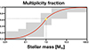
Fig. 2. Sketch representing the multiplicity fraction for stars and brown dwarfs (red line), with the uncertainties summarising numerous observational studies in the literature (grey boxes). More than half of the solar-like stars situated near the yellow star symbol are expected to have a companion. The figure was inspired by Moe & Di Stefano (2017).
-
They are all slow rotators from early in their life as they are subject to efficient magnetic braking during their core hydrogen burning phase. As we detail in the next sections, this implies that the impact of rotation on the modelling of their oscillations is in the easiest regime of the frequency domain. We come back to this important aspect throughout this review.
None of these five aspects is valid for moderate to fast rotators of intermediate to high mass. We define stars born with 1.3 M⊙ ≤ M ≤ 8 M⊙ as intermediate-mass stars and those with M > 8 M⊙ as high-mass stars. For the pulsators in these two mass regimes we do not have a main-sequence calibrator like the Sun, whose helioseismology (Christensen-Dalsgaard 2002) has been essential to guide similar applications to low-mass stars.
Though a minority compared to their low-mass colleagues, stars born with M ≥ 1.3 M⊙ deliver a major fraction of the energy and heavy elements to galaxies and to the Universe as a whole. For this reason, and given the fast progress of asteroseismology for this under-represented category of fast rotators, we dedicate most of this review to asteroseismic applications of stars born with intermediate or high mass. In the next section we clarify what we mean by moderate and fast rotation.
Figure 2 shows the binary fraction for stars and brown dwarfs. This figure makes it clear that we cannot ignore stellar multiplicity in a review focusing on the asteroseismology of intermediate-and high-mass stars. In particular, close binarity dominates the evolution of the most massive stars (Sana et al. 2012, 2013, 2014). While this was firmly established observationally a decade ago, it is recognised that binary evolution theory is still affected significantly by the major uncertainties occurring in the theory of single-star evolution (Marchant & Bodensteiner 2024). Hence, this must be given the highest priority, and asteroseismology is the optimal way to do so (Aerts 2021). We touch upon various aspects of binarity and multiplicity for asteroseismic studies in Sects. 5 and 6. The class of sub-dwarfs is discussed briefly in Sect. 7. It deserves special attention in this respect as the binary fraction is high (Han et al. 2003; Hu et al. 2008; Vos et al. 2017, 2019). In fact, all sub-dwarfs originate from binary interactions because the seemingly single class members can only be understood in terms of a common envelope phase resulting in a merger (Heber 2009). Due to the efficient loss of their envelope, the core-helium burning sub-dwarfs are of low mass in their current phase of evolution (about 0.5 M⊙). Those with oscillations reveal high-frequency modes with periods much shorter than their rotation and/or orbital period (see Lynas-Gray 2021, for a review). We also briefly touch upon merger seismology for higher mass objects, offering a way to hunt for such stars asteroseismically. Section 8 is dedicated to future outlooks, putting emphasis on Gaia’s role in asteroseismology.
Rather than trying to be exhaustive in reviewing the progress of asteroseismology, this paper takes the approach of offering the non-expert reader highlights from the recent literature based on prominent case studies. This way, we illustrate what can be achieved with current and future data and theoretical developments. The plan of the paper is as follows. We provide an accessible introduction to asteroseismology in Sect. 3, touching upon the wave equations representing stellar oscillations and the accompanying frequency regimes. Section 4 covers recent applications of asteroseismology of single stars, starting with the Sun and gradually increasing the level of complexity in the mode computations as the ratio of the oscillation mode periods to the rotation period increases. In Sect. 5 we highlight how model-independent dynamical masses and radii help asteroseismology, before moving on to tidal asteroseismology in Sect. 6 and sub-dwarf and merger seismology in Sect. 7. We end the paper with an extensive outlook for the bright future of asteroseismic applications to stars of intermediate and high mass from combined Gaia data, survey spectroscopy, and ongoing TESS or future PLATO space photometry. There is a pertinent need for new theory and better modelling tools in order to interpret the oscillations of fast rotators and close binaries up to current measurement precisions.
3. Asteroseismology’s unique probing power
This review is focused on applications of asteroseismology to rotating stars, while omitting jargon so as to make it easily accessible. A major focus is put on future prospects and opportunities (see Fig. 1). Hence, we only introduce concepts and equations that are absolutely necessary to keep the text self-contained. We refer to the monographs by Unno et al. (1989) and Smeyers & Van Hoolst (2010) for full derivations of the oscillation equations. Further, we point to Aerts et al. (2010) and Basu & Chaplin (2017) for extensive descriptions of the analysis tools and the principles of stellar modelling in the modern era of space asteroseismology.
Here it is enough to know that non-radial oscillations lead to periodic deviations from the equilibrium structure of the star. Each mode moves the fluid elements away from the position they would have without any seismic activity. Each mode displaces the fluid elements with a periodicity corresponding to the mode’s frequency and its nodes. Since this perturbs a three-dimensional (3D) body, three numbers are required to describe the geometry of each mode. Two of these are called ‘wavenumbers’ and stand for the number and position of nodal lines at the stellar surface with respect to the symmetry axis of the oscillations. In the case of a spherical star in equilibrium that gets perturbed by the modes, these wavenumbers are usually denoted as (l, m), which characterise the nodal lines of a spherical harmonic function Ylm(θ, ϕ) used to describe the angular part of the displacement vector due to the mode. Assignment of the third number, n, is connected with the number of nodes in the radial component of the eigenfunction. It is more involved than the cases of l and m because it depends on the dominant restoring force of the oscillations (Aerts et al. 2010). For the simplest case of radial (l = 0) oscillations, the pressure gradient is the restoring force, and hence these are acoustic eigenmodes (or p modes) of the star. The radial mode with the n-th lowest eigenfrequency has n nodes in its displacement vector. Since the centre of the star is a node, n − 1 nodes occur between the centre and the surface of the star and one speaks of the (n − 1)-th overtone, while the radial mode having only a node in the star’s centre is called the fundamental mode. The classifcation of non-radial modes (l ≠ 0) in terms of their overtone is considerably more complex because additional restoring forces, such as buoyancy, come into play. We refer to Takata (2012) for a detailed mathematical description of mode classification in terms of the overtone n, denoted here as pn and gn for p and g modes of radial order n, respectively. We end this part on the mode numbers by pointing out that the white dwarf community has historically denoted the radial order as k instead of n.
3.1. Stellar evolution models in equilibrium
Modern asteroseismic modelling applications require numerical solutions of the relevant oscillation equations described in the next sub-section. The modelling hence relies on realistic unperturbed background stellar models. Any fluid element inside a rigidly rotating star is characterised by its position vector r with respect to the star’s centre and the time coordinate t measured since the birth of the star (called the zero age main sequence or ZAMS defining time zero). The fluid elements have to fulfil the equations of stellar structure at any time during the star’s evolution (see the monograph on models of rotating stars by Maeder 2009, for the derivations and solutions of these equations).
Since we wish to introduce and discuss the dynamical properties of stellar oscillations, we limit ourselves to a description of the equation of motion, and we focus on a rigidly rotating star for now. Expressed in a frame of reference co-rotating with the star’s rotation vector Ω = Ω ez, where ez is the unit vector along the rotation axis, the equation of motion reads
 (1)
(1)
In this equation, ρ is the density, p is the pressure, v is the velocity vector, and Φ is the gravitational potential fulfilling the equation ∇2Φ = 4πGρ with G the gravitational constant. Aside from the two accelerations due to the pressure and gravitational forces, the two terms aextra represent extra accelerations due to the joint effect of any active forces not spelled out explicitly, one term for forces active inside the star and the other one for forces imposed by external sources. An example of  is the Lorentz force caused by an internal magnetic field or accelerations due to radiative forces resulting in a dust-driven or line-driven stellar wind. Additionally, extra accelerations
  may be caused by external forces such as magnetic fields and/or tides due to one or more companions.
For an unperturbed background model of a single star not subject to any extra forces aside from those due to pressure gradients, gravity, and rotation, the equilibrium state at time t is described by v = 0. In that case, it follows from Eq. (1) that the star is an oblate spheroid flattened due to its centrifugal force (see Espinosa Lara & Rieutord 2013, for an extensive discussion). Most of the current stellar evolution codes simplify the oblateness of stars caused by rotation and describe the gaseous spheroids by using only one spatial coordinate, for instance the distance r from a fluid element to the centre of the star. Thus, any fluid element is characterised by two coordinates, denoted here as (r, t) with t the star’s age.
Almost all the asteroseismic applications discussed in this review are based on such one-dimensional (1D) background models evolving with time, assuming either rigid rotation with constant frequency Ω or shellular rotation (Zahn 1992) for which the rotation frequency only depends on r and not on latitude θ or longitude ϕ. Shellular rotation is denoted here as Ω(r) and results from the assumption of strong horizontal turbulence, forcing a constant rotation rate along isobars. We discuss prospects for asteroseismic applications relying on more realistic yet more complex 2D or 3D background models in the last section.
3.2. The wave equations describing the dynamics of stellar oscillations in a rotating star
Each oscillation mode causes the fluid elements in the star to become displaced from their equilibrium position according to the Lagrangian vector ξ(r, t). In general, the oscillation equations for a rotating star are of the form
 (2)
(2)
where a superscript dot stands for a time derivative and the operators O(i) group all acting forces such that their application represents a collection of terms of i-th order in ξ for i = 1, 2, 3, …. In order to solve Eq. (2), one can take various approximations and approaches, depending on the importance of the Coriolis, centrifugal, magnetic, and tidal forces. The validity of approximations depends strongly on the mode frequency regimes with respect to the rotation frequency, whether or not we have to take into account deformation due to the centrifugal force, and whether we are dealing with rigid or non-rigid rotation. We briefly discuss some of the options, but refer to the references for details.
Asteroseismology is most often applied in a linear framework, where it is assumed that any perturbation of the background equilibrium model stemming from an oscillation mode is sufficiently small to ignore the effects of order higher than one in the displacement ξ in Eq. (2). This means that we can ignore all terms on the right-hand side in Eq. (2). In this case, the equation of motion in Eq. (1) due to the mode ξ is the much simpler version of Eq. (2), namely
 (3)
(3)
where the operator O(1) contains all acting internal forces. If we further write the Lagrangian displacement experienced by a fluid element inside a non-rotating non-magnetic single spherical star at position r and time t due to a periodic linear eigenmode with frequency ω as
 (4)
(4)
the wave equation simplifies to
 (5)
(5)
with O(1) a linear function determined by the equilibrium values and first-order perturbations of the density, pressure, and gravitational potential (e.g. Aerts et al. 2010, Chapter 3). This is the simplest version of the wave equation to solve for a family of linear spheroidal non-radial oscillation modes. We highlight some of the latest findings of helio- and asteroseismology in this simplest approximation in Sect. 4.1.
Versions of non-linear theory of non-radial oscillations based on Eq. (2) have also been developed, up to second (Dziembowski 1982; Buchler & Goupil 1984), third (Van Hoolst & Smeyers 1993; Buchler et al. 1995; Mourabit & Weinberg 2023), or fourth (Van Hoolst 1994) order in ξ, while ignoring the rotation of the star or by considering it to cause only a small perturbation. However, applications of asteroseismic modelling based on higher-order (in ξ) theory are scarce. They occur for oscillation modes in white dwarfs (Zong et al. 2016a), sub-dwarfs (Zong et al. 2016b), red giants (Weinberg & Arras 2019; Weinberg et al. 2021), and a δ Sct star (Mourabit & Weinberg 2023), all of which treat rotation as a small perturbation for the computation of the displacement vectors. Modelling of tides in close binaries may also require non-linear non-radial oscillation theory to solve Eq. (2) when linear tides do not provide a sufficiently accurate description, as theorised by Weinberg et al. (2012), Ogilvie (2014).
A different aspect of simplifying Eqs. (1) and (2) deals with the treatment of rotation, notably the importance of the Coriolis and centrifugal forces and how they compare to the Lorentz force. The rotational effect in the equation of motion leads to terms up to Ω2. The Coriolis force creates vorticity. It may become the dominant restoring force instead of the pressure force or gravity. Hence, one encounters additional families of modes, which do not exist in non-rotating stars. A well-known example from both geophysics and astrophysics involves the family of toroidal modes. For a pedagogical derivation and discussion of the various types of mode families in rotating stars, we refer to Townsend (2003a).
The strategy used to compute oscillation modes in a rotating star depends entirely on how the mode periods compare to the rotation period. If these two are of comparable order, the rotation cannot be treated as a small effect to compute ξ (see also the next section). If the rotation happens on a much longer timescale than that of the oscillations, the rotational effects can be treated in a perturbative approach. This is typically a good strategy when the rotation period is at least ten times longer than the mode periods. In such a case, perturbation theory for proper computation of ξ can be developed up to any order in ε ≡ Ω/ω, where ε is a small expansion parameter for computing the displacement in the form ξ = ξ0 + ε ξ1 + ε2 ξ2 + … . We note that this methodology only makes sense if ε is sufficiently small as an expansion parameter, and hence the modes should have far shorter periods in the frame of reference co-rotating with the star compared to the rotation period. Within such an approach, one must then also decide whether the deformation of the star, which is ∝Ω2, can be ignored or not. If it must be taken into account, the seismic modelling requires a way to incorporate the deformation, either at the level of the equilibrium structure or at the level of the expression for ξ, or both. Often one considers the simplest deformation only at the level of the equilibrium structure, where the contribution to the potential is approximated by its spherically symmetric component (see Eq. (30) in Aerts 2021). Whatever the choice of how to deal with the deformation, one also needs to specify whether and up to what order the terms due to the Coriolis and centrifugal forces couple to each other when computing ξ.
A variety of first-, second-, and third-order perturbative non-radial pulsation theories for the computation of spheroidal and toroidal families of mode solutions is available in the literature, relying on the assumption that all the terms within the operator O(1) as well as the term  in Eq. (2) cause only small deviations from the solutions to Eq. (5) represented by ξ0. We note that the computation of ξ = ξ0 + ε ξ1 + ε2 ξ2 + … from perturbation theory to treat the rotation may involve mode coupling, particularly among spheroidal and toroidal modes, but this is a different matter than adopting non-linear oscillation theory by relying on the right-hand side of Eq. (2). The series ξ = ξ0 + ε ξ1 + ε2 ξ2 + … in perturbation theory used to compute linear modes of rotating stars can be truncated after taking sufficient terms in numerical computations, depending on the envisioned precision required for the modelling application. Perturbative approaches for asteroseismic modelling adhering to the requirement Ω < < ω were developed theoretically long before the modern era of space asteroseismology (e.g. Ledoux 1951; Saio 1981; Gough & Thompson 1990; Dziembowski & Goode 1992, 1996; Soufi et al. 1998; Daszyńska-Daszkiewicz et al. 2002; Karami 2008, each of which containing a lot of technical details).
In summary, for each particular asteroseismic modelling application, proper balancing between the acting forces in Eqs. (1) and (2) is necessary in order to decide upon the best theoretical formalism and the most suitable numerical approach to calculate the oscillation modes. The choice between a perturbative or non-perturbative approach to calculate the modes of equilibrium models depends entirely on the frequency regime of the detected modes under investigation, notably the value of ε (see e.g. Ballot et al. 2010, 2013). This is the major reason why we organise the applications discussed in the following sections according to the regimes of the frequencies of the detected oscillations.
3.3. Oscillation mode frequency regimes
All stars rotate, even if many do so slowly, by which we mean that their rotation velocity is only a small fraction (up to 10%) of their critical break-up velocity. The seemingly simple concept of break-up velocity, defined as the velocity of fluid elements at the stellar equator high enough to overcome the gravitational attraction, is non-trivial. The centrifugal acceleration due to fast rotation can be accompanied by extra outward forces, making it easier to overcome the inward force of gravity. An example is the case of a radiation-driven wind (Kudritzki & Puls 2000) or the tidal pull by a companion (Fuller et al. 2019), helping matter to escape more easily from the star compared to the case without such helpful forces.
In this review we focus on intermediate- and high-mass stars with sufficient detected and identified non-radial oscillation modes in terms of their angular mode dependence to scrutinise stellar equilibrium models. This means that the identified modes allow quantitative measurements of the internal rotation profile and possibly the internal magnetic field. With a few exceptions, asteroseismic modelling based on sufficient modes to achieve this in such types of stars has only begun in the space asteroseismology era. At the time of writing, stars fulfilling these requirements have a mass typically below 25 M⊙ for the core-hydrogen burning phase, and lower for the hydrogen-shell or core-helium burning phases. We therefore ignore the effect of a dynamical wind and rely on a static outer boundary condition to compute the oscillation modes via Eq. (2). We treat the case of tidal forces due to a close companion in Sect. 6.
We use the definition of the Keplerian angular critical frequency given by
 (6)
(6)
where M is the mass and Req the equatorial radius of the star, in comparison with the star’s oscillation frequencies in a co-rotating frame. The equatorial radius of a star is most often unknown, unless the star has a well-resolved interferometric image such as the fast-rotating stars Altair (Domiciano de Souza et al. 2005; Monnier et al. 2007; Bouchaud et al. 2020), Rasalhague (Monnier et al. 2010), Vega (Monnier et al. 2012), or Archenar (Domiciano de Souza et al. 2014). Lack of knowledge of Req is one of the reasons why the critical rotation rate adopted in calculations often corresponds to the Roche critical frequency, defined as
 (7)
(7)
with Rpole the star’s polar radius. These two expressions are not the same because the polar radius only equals 2Req/3 when the actual critical rotation velocity of the star is reached (which is never the case as the star would no longer exist). For a more elaborate discussion on the relationship between  and
and  , we refer to Rieutord et al. (2016). In citing the results below, we explicitly mention the definition adopted by the authors for the critical rotation frequency whenever available.
Here we define a star as a slow rotator if its rotation frequency is less than 10% of its Keplerian critical frequency, a moderate rotator if it has a rotation frequency between 10% and 70% of its Keplerian critical frequency, and a fast rotator if its rotation frequency is above 70% of the Keplerian critical frequency. This may differ substantially from the definitions adopted by spectroscopists, who usually only consider vsin i to decide whether a star is a fast or a slow rotator. As an illustration of this, we computed  and
and  for the 12 M⊙β Cep star HD 192575, which has a measured vsin i ≃ 27 km s−1 and whose oscillation spectrum is shown in Fig. 6 (discussed further in the text). Based on the high-resolution spectroscopic estimate of vsin i, one would be tempted to classify this star as a slow rotator because most B-type stars have 5 to 15 times higher vsin i. However, asteroseismologists are not hampered by the unknown sin i factor as they measure Ω directly from the oscillation frequencies (see Pedersen 2022a, for a sample of B stars). For HD 192575 this leads to an equatorial rotation velocity between 75 and 100 km s−1 and an inclination angle between 10° and 30° (Burssens et al. 2023). Moreover, what matters for asteroseismic modelling is the ratio of twice the rotation frequency and the oscillation mode frequency in a frame of reference co-rotating with the star, called the mode spin parameter and defined as s ≡ 2Ω/ω. From the asteroseismic modelling of this star by Burssens et al. (2023), we find that the star’s rotation frequency at the position of the μ-gradient zone adjacent to the receding convective core has
  and
and  , while its radiative envelope near the surface rotates at
  and
and  . The spin parameters of the dipole and quadrupole modes range from about 5% to 20%. Hence, we classify this star as a moderate rotator because second-order rotational effects should not be neglected to achieve an optimal interpretation of its observed rotationally split mode frequencies shown in Fig. 6. We come back to the unique asteroseismic study of this star as a key example of low-order p- and g-mode asteroseismology of a supernova progenitor in Sect. 4.2.
Aside from the mode frequency ω and the star’s rotation frequency Ω (assuming rigid rotation for now), several more frequencies connected with the internal dynamical properties of a star are of importance. The cavity of the p modes has a characteristic acoustic frequency for each of the modes, known as the Lamb frequency Sl and defined as
 (8)
(8)
with c(r) the local sound speed. Pressure modes of degree l are only propagative in the region where ω > Sl. Gravity modes, on the other hand, are only propagative if their frequency is below the Brunt-Väisälä frequency N, defined as
 (9)
(9)
with Γ1 the first adiabatic exponent:
 (10)
(10)
Finally, some layers in stars may be subject to a magnetic field, whose origin, evolution, and properties vary from star to star. Such layers experience plasma waves restored by the Lorentz force. These waves are characterised by their Alfvén frequency, ωA, corresponding to a wave speed
 (11)
(11)
with B the magnetic field, k the wave vector, and μ0 the permeability.
Figure 3 assembles all the introduced frequencies into a single axis representing a classification of the types of waves corresponding to their dominant restoring force. The dynamical properties of the resonant eigenmodes depend on the relationship between their frequencies ω and the Lamb, Brunt-Väisälä, rotation, and Alfvén frequencies. The types of approximations that can be made to compute the eigenmode frequencies ω via Eq. (3) for  are also indicated in the figure. In particular, given that almost all stars rotate with periods shorter than a decade, we make a distinction of their waves in the sub-inertial and super-inertial regimes, defined as those having spin parameter s ≡ 2Ω/ω above or below 1. Throughout the life of a star, the frequencies indicated in Fig. 3 change appreciably. We refer to the extensive Table A.1 in Aerts et al. (2010) for typical values of mode periods for all the different types of pulsators, along with typical ranges of the dominant mode amplitudes, luminosities, and effective temperatures corresponding to their excitation mechanism and evolutionary stage as indicated by their position in the HRD discussed in Fig. 1 of Aerts (2021).
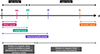 |
Fig. 3. Axis showing various frequencies of relevance inside a rotating star, notably the Lamb frequency for a wave of degree l denoted as Sl, the Brunt-Väisälä frequency N, the rotation frequency Ω, and the frequency due to Alfvén waves ωA. The relevant frequency regimes for different types of waves are indicated, as well as the regimes where particular forces can (or cannot) be treated perturbatively in the computation of oscillation modes. Waves in the sub-inertial regime have spin parameter s ≡ 2Ω/ω > 1, while waves in the super-inertial regime are characterised by s < 1. The indicated frequencies change throughout the evolution of the star. The figure was inspired by the scheme in Mathis & de Brye (2011) and is adapted from the version in Aerts et al. (2019), by Clio Gielen. |
We emphasise here that the frequencies of gravity modes or internal gravity waves of a moderate or fast rotator detected by an observer in the inertial frame of reference characterised by (r, θ, ϕ, t) are appreciably different from the frequencies computed for a reference frame co-rotating at frequency Ω with the star characterised by (r′,θ′,ϕ′). This is due to purely geometrical reasons, even without taking into account the Coriolis or centrifugal forces. We can easily understand this based on the simplest case of a slow rotator, for which the geometry of an eigenmode can be approximated by a spherical harmonic, Ylm(θ′,ϕ′). In terms of time dependence, the transformation from the co-rotating to an inertial reference frame follows from
 (12)
(12)
such that a frequency in the co-rotating frame, ωcorot will be detected as ωinertial = ωcorot + m Ω by an observer. While this geometrical shift with m Ω may be relatively small for high-frequency modes of a slow rotator, the effect is large for low-frequency modes of a fast rotator. As an example, let us consider typical low-degree prograde (m > 0) or retrograde (m < 0) modes of slowly pulsating B (SPB) or γ Doradus (γ Dor) stars. These modes typically have frequencies of about 5 to 20 μHz in a co-rotating frame of reference. These mode frequencies get shifted by m Ω in an observer’s inertial frame, as illustrated in Fig. 4. Following the measured rotation frequencies Ω for these two classes of pulsators (cf. Fig. 6 in Aerts 2021), this geometrically based shift can reach values up to 30 μHz and −30 μHz for prograde and retrograde dipole (l = 1) modes, respectively. Moreover, the frequency shifts increase dramatically as the mode degree increases, given that m ∈ [ − l, l]. In addition, the Coriolis force induces extra frequency shifts, lifting the degeneracy with respect to zonal (m = 0) mode frequencies in the co-rotating frame. These shifts must also be taken into account, in addition to the geometrical shifts. It is then clear that one cannot make meaningful comparisons between observed frequencies as in Fig. 4 and their theoretical predictions in a co-rotating frame without applying the proper frequency shifts between the reference frames. This is an essential point of attention for asteroseismic modelling of moderate and fast rotators. Such modelling requires the identification of the azimuthal orders m in order to interpret the collective effect of all the numerous detected oscillations in observations of rotating stars whose modes and waves cannot be treated perturbatively with respect to the Coriolis force (see Fig. 3).
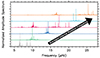 |
Fig. 4. Gallery of amplitude spectra deduced from 4 yr Kepler light curves for six dipole prograde g-mode pulsators of intermediate mass. The graph illustrates typical frequency shifts in an inertial frame of reference connected with (l, m)=(1, +1) modes in such stars. The lower curve is for the only slow-rotating SPB star with detected rotationally split triplets, KIC 10526294. This star’s 19 dipole mode triplets were discovered by Pápics et al. (2014) and subjected to rotation inversion, following the forward asteroseismic modelling of its zonal dipole modes by Moravveji et al. (2015). Its internal rotation profile deduced from mode inversions led to a rotation frequency of 0.16 μHz (Triana et al. 2015). The upper curve represents the data for the γ Dor star KIC 9210943, rotating essentially rigidly, with frequency 19.73 μHz near its convective core and 19.70 μHz at its surface (Van Reeth et al. 2018). |
In the following sections we discuss some applications of asteroseismology, with an emphasis on moderate to fast rotators. However, we begin with slow rotators for ease of understanding and to focus on some recent highlights for such stars. We discuss applications for various types of stars, giving descriptions of case studies with the aim to encourage future applications.
4. Applications of asteroseismic modelling to single stars
In order to understand the asteroseismology of fast rotators, it is convenient to first recall how it works for slow rotators. After a brief description of the basic principles of asteroseismic modelling, we recall some of the challenges involved in the probing of the Sun’s internal sound speed from its acoustic modes. Subsequently, we provide some recent topical updates of asteroseismology applied to slowly rotating low-mass stars before moving on to faster rotators. Throughout this section, Fig. 3 will be our guide for the applications. We start on the right with high-frequency acoustic oscillations and will gradually shift to the left along the frequency axis.
4.1. Principles of asteroseismic modelling of slow rotators
The linear free oscillation modes of a non-magnetic single star whose oblateness caused by the centrifugal force can be ignored are obtained by solving the simplified version of Eq. (3), that is, by setting  and ignoring all forces aside from gravity and the pressure and Coriolis forces. The wave equation then becomes
 (13)
(13)
where ω is the frequency in the co-rotating frame for simplicity of notation. The full expression of the linear operator O(1) is omitted here for brevity, as we do for all theoretical expressions for the eigenmodes in the rest of this review. It can be found in Eq. (3.340) of Aerts et al. (2010). For modes in the super-inertial frequency regime, one can treat the Coriolis force in Eq. (13) perturbatively, while it has to be taken into account in full for moderate and fast rotators (see Fig. 3). In the applications spelled out below, we gradually upgrade towards higher complexity caused by rotation, focusing on pedagogy rather than completeness in quoting the literature.
Simplifying maximally to zeroth order in Ω (i.e. no rotation) implies the full separability of Eq. (13) in terms of spherical coordinates and time as it reduces to Eq. (5). We thus find a family of spheroidal oscillation modes with frequencies ωnl. A degeneracy with respect to the azimuthal order m occurs, and the time-independent part for the Lagrangian displacement, ξ(r), can be written in terms of spherical harmonics, Ylm. The expression for ξ(r, θ, ϕ, t) is derived in full detail and spelled out explicitly in standard books treating non-radial oscillations of stars (see Unno et al. 1989 and Aerts et al. 2010, Chapter 3, Eq. (3.132)).
Forward asteroseismic modelling of slow rotators to estimate their basic stellar parameters such as mass, radius, core mass or envelope mass, and age is usually done by matching the observed frequencies, ωnl, of identified zonal (m = 0) modes of degree l and radial order n, with those predicted from grids of 1D stellar evolution models. Such grid modelling is minimally a 4D optimisation problem as any stellar evolution code requires the mass, initial chemical composition (any combination of the mass fractions of hydrogen X, helium Y, or the metals Z), and age as input in order to compute the stellar structure for that moment in the star’s evolution. However, the problem to solve is in practice of much higher dimension, as numerous free parameters occur in the codes due to limitations in our knowledge of the input physics and/or simplifications of inherently 3D physical macroscopic processes into 1D prescriptions. While this 3D-to-1D simplification is fine for gravity, thermodynamics, and the microphysics (e.g. nuclear reactions, equation-of-state, atomic diffusion), it gives bad approximations for macroscopic transport processes due to rotation, magnetism, and tides. Hence, for computations with codes assuming the stellar structure models to be described in 1D, one is forced to introduce free parameters summarising the effects of these 3D macroscopic phenomena. One thus rapidly ends up in a high-dimensional parameter space for the fitting of the oscillation frequencies; there are currently ample opportunities to attack the regression problem with machine-learning tools (cf. Bellinger et al. 2016; Hendriks & Aerts 2019; Bellinger 2019, 2020; Angelou et al. 2020; Hon et al. 2020).
4.1.1. A few updates on solar modelling
The dimensionality of the regression problem involved in stellar modelling can be reduced appreciably if proper calibrations for the input physics or model-independent ranges for the parameters are available. We discuss this latter aspect for intermediate- and high-mass stars in Sect. 5. For slow-rotating low-mass stars, one often freezes the input physics, notably the mixing length parameter used in time-independent convection theory, to parameter values calibrated from helioseismology. While doing so, it must be kept in mind that the models may include extra forces in the term  in Eq. (1) that may be operational in the stars of the application, while being absent or less important for the Sun. We illustrate here that, even for the star we know best, helioseismology is still an active yet specialised sub-field of asteroseismology, for which the slow solar rotation matters in improving the dynamics in the Sun.
In terms of physical ingredients, the progress in solar models compared to the famous Model S (see Christensen-Dalsgaard et al. 1996, for details) has been great (Christensen-Dalsgaard 2021). However, the physical description for two regions inside the Sun, notably the base of the convective envelope and the surface layers, require improvements. The properties of the internal rotation of the Sun as summarised by Thompson et al. (2003, Fig. 7) and updated by Christensen-Dalsgaard & Thompson (2007) reveal a decrease in the surface rotation frequency from about 450 nHz at the solar pole (zero latitude) to about 330 nHz at latitude 75°. The level of latitudinal differentiality decreases from the solar surface to the base of the convection zone situated at a fractional radius of r/R⊙ = 0.713. The transition region between the differentially rotating convective envelope and the quasi-rigidly rotating (at about 440 nHz) radiative interior is called the tachocline.
Figure 5 illustrates the deviations between the squared sound speed profile of the true Sun delivered by its thousands of identified acoustic modes and those based on some of the best models. The agreement between the 1D solar models and helioseismic data is better than 1.5%. However, the remaining discrepancies between theory and observations are highly significant due to the extreme precision of the observations. Aside from the ongoing controversy between the ‘old’ and ‘new’ Sun in terms of its surface abundance determinations (Buldgen et al. 2023, 2024), the deviations between the Sun and the current solar models in the tachocline are likely linked to the interplay of processes on microscopic and macroscopic scales. This is a question of limited knowledge of opacities (Bailey et al. 2015), of mixing processes at the base of the convection zone (Baraffe et al. 2022), and of angular momentum transport (Eggenberger et al. 2022a), among other aspects.
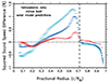 |
Fig. 5. Squared sound speed differences between helioseismic observations and predictions based on three models of the Sun from oscillation mode structure inversions. The errors along the y-axis are often smaller than the symbol size. The numerous small regions indicated by the horizontal bars along the x-axis represent the intervals in fractional radius over which the localised mode kernel averaging was done for the inversions. Models delivering perfect agreement with the solar oscillations would coincide with the dotted horizontal line. The vertical dashed line indicates the helioseismic derivation of the base of the solar convection zone. The agreement between the observations and the best model predictions has degraded since the era of Model S (Christensen-Dalsgaard et al. 1996), despite immense improvements in the description of the physics in terms of the equation of state, opacities, and transport of chemical elements in the solar interior, as explained in Christensen-Dalsgaard (2021). This downgrade is due to the adopted solar surface abundances measured by Asplund et al. (2021), who relied on 3D non-local thermodynamic equilibrium (NLTE) atmosphere models and their line predictions leading to a ratio of metals to hydrogen of Z/X = 0.0187 based on the solar calibration carried out in Buldgen et al. (2024), while LTE abundances from 1D atmosphere models from Grevesse & Noels (1993) were used for the older red curve from Model S. The blue curve results from averaged 3D NLTE-based abundances by Magg et al. (2022) leading to Z/X = 0.0225, and was computed by Dr. Gaël Buldgen relying on the physical descriptions adopted in Buldgen et al. (2023) and Buldgen et al. (2024). The figure was produced from data kindly made available by J. Christensen-Dalsgaard (red curve) and G. Buldgen (cyan and blue curves). |
All 1D models of the Sun and of low-mass stars also suffer from the what is known as the ‘surface effect’ (see the lack of points between r/R⊙ = 0.97 and 1 in Fig. 5). This represents an offset between measured frequencies of identified modes and those predicted by the best 1D solar models of the order of a few μHz, which is much larger than observational uncertainties. The offsets are mode dependent and increase for increasing radial order of the acoustic modes (higher mode frequencies). Improving envelope models of the Sun and of low-mass stars requires a full 3D description incorporating the interplay between acoustic oscillations and 3D time-dependent convection (Mosumgaard et al. 2020), keeping in mind the non-adiabaticity of the gas (Houdek et al. 2019).
Novel 3D simulations of the whole convective solar envelope, including shear-driven magnetic buoyancy due to rotation in the tachocline, provide new insights into the local mixing it induces (Matilsky et al. 2022; Duguid et al. 2023). This illustrates that rotation matters, even for slow rotators such as the Sun. In addition, thanks to long-term monitoring from space by the Heliospheric and Magnetic Imager on board NASA’s Solar Dynamics Observatory (SDO, Pesnell et al. 2012), a novelty was introduced into helioseismology in 2018. Aside from the well-known spheroidal high-frequency acoustic modes occurring in the high-frequency regime to the right in Fig. 3 and used in Fig. 5, toroidal inertial modes restored by the Coriolis force with frequencies below twice the solar rotational frequency were discovered in the SDO data by Löptien et al. (2018). They are related to equatorial Rossby modes as well as high-latitude inertial modes (Gizon et al. 2021). These recently discovered retrograde modes open up inertial-mode helioseismology, an exciting new way to probe the dynamics of the rotating tachocline and solar envelope (Bekki et al. 2022). We come back to Rossby modes in Sect. 4.4, where we point out that such modes were already discovered in numerous rapidly rotating stars of intermediate mass years prior to those found in the Sun.
To conclude, despite the challenges shown in Fig. 5 the precision of the solar models at the level of 1.5% or better is a remarkable achievement of helioseismology. Additional limitations for models of fast rotators will be discussed as of Sect. 4.3.
4.1.2. Updates on forward modelling of slow rotators
For the distant stars, we cannot rely on high-degree (e.g. l > 4) modes from space photometry, as their effects cancel out when integrating the variability across the visible hemisphere in the line of sight. Forward modelling in such cases relies on observables in addition to the mode signals (Gent et al. 2022), notably spectroscopic and astrometric input to delineate the grids of 1D equilibrium models used for the regression in the modelling of the stellar interior. Spectroscopic effective temperatures and gravities, as well as luminosities from Gaia parallaxes (Gaia Collaboration 2016) have become available for large ensembles of low-mass dwarfs and red giants in the Milky Way. These inferred stellar properties are used in tandem with their seismic observables from CoRoT, Kepler and TESS for galactic studies (see Fig. 1; Anders et al. 2014; Chiappini et al. 2015; Pinsonneault et al. 2018; Zinn et al. 2019, 2020; Claytor et al. 2020; Mackereth et al. 2021; Grunblatt et al. 2021; Zinn et al. 2022). We note the large difference in relative precision between such classical quantities and the seismic observables connected with identified modes (factors 10 to 1000, see Table 1 in Aerts et al. 2019).
The matching between observed and theoretically predicted frequencies of identified modes is mostly done in a Bayesian framework, where the error estimation is often tackled numerically from a Markov chain Monte Carlo approach (Appourchaux et al. 2009; Gruberbauer et al. 2012, 2013; Chaplin et al. 2014; Silva Aguirre et al. 2017). Deducing stellar parameters with high precision for large ensembles is one major asset of asteroseismology (e.g. Stello et al. 2011; Hekker et al. 2011, 2013; Huber et al. 2011, 2012; Davies et al. 2016; Brogaard et al. 2018, 2022; Farnir et al. 2021; Li et al. 2022a, 2023a) as input for other studies in astrophysics (see Fig. 1), notably galactic archaeology (Miglio et al. 2009, 2013, 2021; Stello et al. 2013; Ness et al. 2016, 2019, 2022; Stello et al. 2017; Anders et al. 2017a,b, 2023; Silva Aguirre et al. 2018; Hekker & Johnson 2019; Li et al. 2022a; Hon et al. 2022, etc.), old open clusters (Brogaard et al. 2012; Miglio et al. 2012, 2016; Brogaard et al. 2021), and exoplanetary research where age-dating and star–planet interactions are crucial aspects (Huber et al. 2013; Lebreton & Goupil 2014; Silva Aguirre et al. 2015; Huber et al. 2019; Chontos et al. 2021; Huber et al. 2022). However, the ages of the stars deduced from any method, including asteroseismology, remain dependent on the input physics used to compute the stellar evolution models and their isochrones, no matter how precisely the mass and initial chemical composition of the stars have been derived. For this reason, stellar ages are at best precise, but not necessarily accurate.
The unknown level of internal mixing due to element transport causes a major systematic uncertainty for the age-dating of stars (Salaris & Cassisi 2017), notably for those of intermediate or high mass born with a convective core. As an example, the age-dating of red giants from non-rotating isochrones while ignoring the fast rotation of their progenitors on the main sequence may lead to systematic age uncertainties in the red giant phases of up to 20% (Fritzewski et al. 2024a). However, this effect is often ignored when providing age estimates and their uncertainties for red giants. More generally, the cumulative effect of convective core overshooting during the main-sequence phase, which may partially be caused by rotational mixing and possibly be inhibited somewhat by a magnetic field, is among the most important unknown factors in age-dating, for all levels of internal rotation rates and masses (e.g. Deheuvels et al. 2015; Bellinger 2019; Mombarg et al. 2019; Pedersen et al. 2021; Johnston 2021; Noll et al. 2021; Noll & Deheuvels 2023).
Developing a calibrated theory of transport processes (Mathis et al. 2013) for all stellar masses and across all evolutionary phases is thus a major aim of asteroseismology. This is currently the only feasible method to offer a proper value for the numerous free parameters occurring in 1D implementations of these processes because their parameters change on an evolutionary timescale. Major progress has been achieved to improve internal angular momentum transport, guided by the overarching measured properties of internal rotation across stellar evolution (Aerts et al. 2019). Simulations based on new theoretical ingredients, involving magnetic fields and/or internal gravity waves are successful in explaining the internal rotation rates deduced from high-precision space asteroseismology (Rogers et al. 2013; Rogers 2015; Fuller et al. 2014, 2019; Eggenberger et al. 2017, 2019; Ratnasingam et al. 2020; Takahashi & Langer 2021; Eggenberger et al. 2022b; Moyano et al. 2023). Nevertheless, more work is needed when it comes to the understanding of asteroseismically determined levels of internal mixing for various ensembles of pulsators (Rogers & McElwaine 2017; Deal et al. 2018, 2020; Mombarg et al. 2020, 2022; Pedersen et al. 2021; Varghese et al. 2023). Asteroseismically measured values of envelope mixing assuming a diffusive coefficient for the element transport in the stellar envelope range from 1 cm2 s−1 to 106 cm s−1 (Aerts 2021, Table 1). Both the level and functional form of internal shear mixing is the dominant unknown ingredient affecting the ages and convective core masses of stars across stellar evolution (Van Grootel et al. 2010a, 2010b; Giammichele et al. 2018; Charpinet et al. 2019a; Tkachenko et al. 2020; Johnston 2021; Pedersen et al. 2021; Pedersen 2022b).
Future age-dating of stars with 10% accuracy instead of precision from asteroseismically calibrated transport processes for exoplanet host stars is a challenging aim in the core science programme of the ESA PLATO space mission (Rauer et al. 2024). PLATO also offers an extensive Complementary Science programme open to the worldwide community offering the study of internal rotation, magnetism, and mixing across the entire HRD (see Fig. 1).
Making progress in our understanding of internal mixing due to element transport requires a good knowledge of dΩ(r)/dr. This brings us back to the quest to deduce the internal rotation profile of stars for different phases of their evolution. Taking the Coriolis force in Eq. (13) into account lifts the degeneracy of the mode frequencies with respect to m and gives rise to resolved rotationally split multiplets if the duration of the time series data is sufficiently long compared to the average rotation period of the star. Ignoring terms in Ω2 in the equation of motion and adopting a perturbative first-order approach in Ω for shellular rotation leads to observed frequencies in an intertial frame of reference according to Ledoux splitting (Ledoux 1951) given by
 (14)
(14)
where Knl(r) are the rotational kernels, which can be computed from the identified modes and the equilibrium structure of a 1D stellar model (Aerts 2021, Eq. (45)). This expression includes the geometrical shift introduced in Eq. (12), as well as the Ledoux constant Cnl caused by the Coriolis force (Ledoux 1951). Hence, following Eq. (14), the rotation frequency Ω(r) throughout the stellar interior gives rise to frequency multiplets ωnlm with 2l + 1 components in the line of sight, provided that all the modes in the multiplet are excited to observable amplitude. We note that the latter circumstance is a good assumption for solar-like oscillation modes excited stochastically by envelope convection, but that this is not necessarily the case for heat-driven oscillations, as shown in this era of high-precision space asteroseismology (Aerts 2021). Modes of particular m may not be excited intrinsically by the heat mechanism, but may be pumped up in mode energy from non-linear mode interactions involving the rotation frequency. We give some examples of this below, as measured in fast rotators.
Equation (14) reveals that treating the Coriolis force perturbatively up to first-order creates symmetrical Ledoux splittings for fixed n and l, given that m ranges from m = −l, …, 0, …, +l. Moreover, in the limit of high-order p and g modes, one can show that Cnl ≃ 0 and Cnl ≃ 1/[l(l + 1)], respectively (see Aerts et al. 2010, for a summary of derivations of these approximations). Hence, for such modes, the measured rotational splittings provide a direct estimate of the local rotational profile Ω(r) averaged by the mode energy, since Knl(r) is determined by the square of the mode displacement ξ (see Eq. (45) in Aerts 2021).
The Ledoux rotational splitting in Eq. (14) is a good approximation for the p modes of low-mass dwarfs, for the p modes of sub-giants and red giants, for the p and g modes of sub-dwarfs, and for the g modes of white dwarfs. For most of these pulsators, the oscillation periods range from several minutes to a few hours and are small fractions of the rotation periods ranging from about a day for white dwarfs (Hermes et al. 2017) to several months for red giants (Mosser et al. 2012; Gehan et al. 2018). Aside from a few exceptions, the spin parameters of the modes of all these types of pulsators in the co-rotating frame, 2Ω/ωnlm, put them far into the super-inertial regime (completely to the right in Fig. 3). Almost all of these pulsators are hence slow rotators in our definition, with their forward modelling being done from their m = 0 mode frequencies and the subsequent derivation of Ω(r) from Eq. (14) relying on the best forward seismic model. With the notable exception of the high-order p modes in the Sun-like star η Bootis modelled with inclusion of the centrifugal deformation by Suárez et al. (2010), summaries of asteroseismic modelling results for the slow rotators can be found in García & Ballot (2019), Hekker & Christensen-Dalsgaard (2017), Lynas-Gray (2021), and Giammichele et al. (2022) for low-mass dwarfs, red giants, sub-dwarfs, and white dwarfs, respectively. Homogeneous analyses for the sub-giant phase were somewhat lacking after the Kepler mission finished, but are now also well underway (Ong et al. 2021; Noll et al. 2021), in anticipation of TESS light curves for this evolutionary phase.
4.1.3. Detection of internal rotation and core magnetism in red giants
The CoRoT space mission revealed that red giants are non-radial pulsators (De Ridder et al. 2009). It was a lucky circumstance that the mission programme could not avoid red giants in the observing fields dedicated to exoplanet research. The mode periods roughly range from half an hour to half a day, while the rotation periods of red giants typically range from ten days to hundreds of days. As discussed in the previous section, this implies that rotation can be treated perturbatively following the Ledoux approximation and that modelling can be done from the zonal modes. The CoRoT discovery of non-radial oscillations in red giants allowed the application of age-dating for various areas of the Milky Way (Hekker et al. 2009; Miglio et al. 2009); major advances in galactic archaeology (e.g. Miglio et al. 2013; Chiappini et al. 2015; Montalbán et al. 2021) is one of the important spin-offs of asteroseismology, as indicated in Fig. 1.
Following the theoretical predictions from Dupret et al. (2009) triggered by CoRoT, dipole mixed modes were discovered in CoRoT data of a sub-giant (Deheuvels et al. 2010) and in Kepler data of a red giant (Beck et al. 2011). Subsequently, such modes were found in a whole sample of red giants by Bedding et al. (2011). The latter breakthrough study led to the important capacity to discriminate between stars on the red giant branch (RGB) and in the first or secondary red clump, even though such stars share the same surface properties. This discriminating capacity was also nicely illustrated for red giants in open clusters (Stello et al. 2011) and relies on the fact that the mixed modes have g-mode character in the deep interior of the star, yet are of acoustic nature in the envelope. Figure 3, helps us understand the nature of these modes: the p- and g-mode cavities delineated by the Sl and N symbols come closer to each other as a star evolves from being a dwarf to a red giant. As shown by Dupret et al. (2009), this narrows the zone between N(r) and S1(r) in such a way that the waves can tunnel through both cavities without becoming fully evanescent in the transition zone, thus creating dipole mixed modes that probe the entire star.
Core rotation frequencies were detected from the splitting of mixed dipole modes in a few Kepler red giants after two years of uninterrupted photometric monitoring (Beck et al. 2012). The positive effect of the longer duration of the Kepler light curves beyond two years implied major progress in seismic precision (Hekker et al. 2012). It led to a revolution in the understanding of angular momentum transport from large samples of evolved stars initiated by Mosser et al. (2012), with refined analyses from rotation inversions for a few RGB pulsators by Deheuvels et al. (2012) and red clump giants by Deheuvels et al. (2015). Following the initial breakthroughs, the internal rotation of evolved stars became an industrialised observational science of major importance (e.g. Gehan et al. 2018; Li et al. 2024a).
Meanwhile, space asteroseismology delivered the internal rotation for several thousands of evolved low- or intermediate-mass stars, notably sub-giants and their successors climbing up the red giant branch, as well as giants in the first and secondary red clumps, sub-dwarfs, and white dwarfs. A summary of the rotational properties of about 1200 slow-rotating field stars is available in the review paper by Aerts et al. (2019) and is not repeated here. Figure 4 in that paper, along with the updated figures with measured internal rotation rates until the end of 2019 in Aerts (2021), place the internal rotational properties of low- and intermediate-mass stars in a global evolutionary picture. This revealed that the angular momentum of the core of helium burning red giants is in agreement with the angular momentum of white dwarfs.
The major new insight from asteroseismology regarding internal rotation across stellar evolution is that the level of radial-differential rotation of single dwarfs of low and intermediate mass is low during their longest phases of evolution, when they fuse hydrogen into helium and helium into carbon and oxygen. As discussed in Aerts et al. (2019), who summarised all results obtained until mid-2018, any explanation of this asteroseismic picture of stellar evolution requires more efficient transport of angular momentum during these phases than anticipated prior to Kepler space asteroseismology. Said differently, much stronger coupling between the convective core and envelope occurs during the two central burning stages of intermediate-mass stars, while strong radial-differential rotation with a factor up to 20 for the core-to-envelope rotation rates occurs during the RGB (Li et al. 2024a). New theories to address this too low angular momentum transport in models of stars with a convective core have been developed. One way to increase the angular momentum transport while such stars evolve is to include internal gravity waves in the models. The occurrence of such waves was already proposed as an efficient way to transport angular momentum in low-mass stars like the Sun by Charbonnel & Talon (2005), Rogers & Glatzmaier (2006) and in high-mass stars by Rogers et al. (2013).
Another way to achieve higher angular momentum transport in models is by including magnetic effects. The existence of internal magnetic fields in red giants was already inferred by Fuller et al. (2015) as an interpretation for depressed dipole mixed modes found in Kepler data for a small fraction of red giants. The accompanying study by Cantiello et al. (2016) showed that a magnetic greenhouse effect may be operational in red giants, turning g modes trapped in the core into Alfvén waves. The mode damping requires internal magnetic field strengths above about 105 G, as confirmed by the theoretical predictions in Loi & Papaloizou (2017). A test of this greenhouse scenario for earlier phases of stellar evolution was developed by Stello et al. (2016), namely about half of the F dwarfs should have a strong internal magnetic field during their main-sequence phase. So far, it has not been possible to test this hypothesis from a representative asteroseismic population of F dwarfs, but internal magnetic field strengths of the 37 best modelled Keplerγ Dor pulsators inferred by Aerts et al. (2021) are in agreement with the scenario by Fuller et al. (2015) keeping in mind the minimal field strengths deduced by Cantiello et al. (2016).
Although the interpretation by Fuller et al. (2015) was contested by Mosser et al. (2017), the presence of internal magnetic fields in a fraction of red giants is no longer a hypothesis. An observational breakthrough was achieved by Li et al. (2022b) and by Deheuvels et al. (2023), who found evidence of the presence of such fields inside the cores of respectively 3 and 11 red giants from 4 yr Kepler light curves. Li et al. (2022b) detected the core magnetism from the occurrence of asymmetrical rotational splittings in the triplets of mixed dipole modes. They interpreted this asymmetry as being due to the small effects induced by the Lorentz and Coriolis forces on the modes. In their approximation, the terms caused by 2 Ω × v and the magnetic force in  are considered small compared to those due to the gas pressure gradient and gravity in Eq. (1), as confirmed by their numerical computations. Elegant analytical and numerical work to interpret the observational findings in the adopted approximation was offered by Li et al. (2022b, see the Supplementary Material) and by Mathis & Bugnet (2023) for various magnetic field topologies, following earlier theoretical studies on the effect of magnetism on modes of red giants by Loi & Papaloizou (2018), Gomes & Lopes (2020), Loi & Papaloizou (2020), Loi (2020a,b,2021), Bugnet et al. (2021), Bugnet (2022). Deheuvels et al. (2023), on the other hand, inferred the presence of a core magnetic field in 11 RGB stars from the effect of the Lorentz force on the frequencies of zonal dipole modes. These 11 red giants do not reveal asymmetries in their dipole mode splittings. Rather, the Lorentz force affects the dipole zonal mode frequencies of consecutive radial order. The effect depends on the strength of the magnetic field and allows us to deduce lower limits on the core field strengths. As such, Deheuvels et al. (2023) found fields of 40 kG to 610 kG for these 11 stars. One of them, KIC 6975038, has depressed dipole modes, lending further support to the original interpretation of a magnetic greenhouse effect by Fuller et al. (2015).
Meanwhile, Li et al. (2023b) detected a core magnetic field from asymmetrical splittings in 13 of the ∼1200 red giants with detected dipole mixed mode triplets found in the sample of 8000 compiled by Yu et al. (2018) and Gehan et al. (2018). The way the authors selected these 1200 RGB stars disfavours such stars with depressed dipole modes, as well as stars in an advanced stage of evolution along the RGB. The average core magnetic field strengths of these 13 stars range from 20 to 150 kG, representing a range from 5% to 30% of the critical field strength above which magneto-gravity waves are dissipated in the core rather than being propagative (Fuller et al. 2015; Rui & Fuller 2023). The detected fields were found to have a variety of horizontal field geometries. The core magnetic fields detected in less than 2% of the Kepler red giants with dipole mixed modes by Li et al. (2023b) and Deheuvels et al. (2023) are important to improve stellar evolution models. The low fraction found in the large homogeneous database of the Kepler 4 yr light curves does not necessarily imply the absence of a field for the majority of stars as the fields may remain undetected for large parts of the evolution. The field strengths were found to decrease as the cores of the stars shrink along their evolutionary path. The magnetic red giants have core rotation properties fully in line with those of the thousands of red giants without detected magnetic signatures. Both findings suggest that the magnetic fields do not cause much extra transport of angular momentum compared to the case of a non-detectable magnetic field. The sample of red giants with detected core fields is currently too small to make strong general conclusions. The effects of the core fields on internal mixing, if any, remain to be studied given the recent character of these discoveries. This may help to assess whether the magnetic field has any effect on element transport as the red giants evolve.
4.2. Asteroseismology of supernova progenitors: Low-order p and g modes in β Cep stars
Moving somewhat to the left on the frequency axis in Fig. 3, we find moderate rotators among the β Cep stars, such as HD 192575 already discussed above. The β Cep stars are dwarfs or (super)giants of spectral type O or early B with masses roughly in the range 8 to 25 M⊙. They are hence precursors of supernovae. This class of pulsators has always played a special role in asteroseismology, and this is no different in this review. As early as 1902, Frost (1902) discovered radial-velocity variations for the prototype of the class, the star β Cephei. At that time, the only explanation was that the star is a spectroscopic binary. Although the variability of tens of similar stars was misinterpreted in terms of orbital motion for about half a century, a breakthrough was achieved thanks to the three periodicities found in the radial-velocity time series for the class member β CMa (Struve 1950; Van Hoof & Struve 1953). These properties in fact led Ledoux (1951) to write his breakthrough paper on non-radial oscillation modes in a rotating star, introducing the concept of rotationally split multiplets due to the joint effect of the Coriolis force and the projection in the line of sight for an observer, as discussed in Sect. 3.3. Even though we know today that Ledoux’s interpretation of the variability of β CMa was wrong (e.g. Mazumdar et al. 2006, for a modern asteroseismic interpretation), it led him to derive a general description of the observed characteristics of non-radial oscillations in a rotating star, which is the one still in use today for slow rotators with modes in the super-inertial regime.
Rotational splitting following Eq. (14) applied to 21 years of multi-colour photometric monitoring led to the first asteroseismic detection of non-rigid rotation in a star other than the Sun (the β Cep star HD 129929, Aerts & De Cat 2003; Dupret et al. 2004). In terms of modes, the β Cep stars reveal low-order p and g modes with periodicities of several hours, while their rotation periods cover the range from more than 100 d down to a considerable fraction of their critical rotation period. None rotate close to critical (Stankov & Handler 2005), however, so following our definition they are slow to moderate rotators.
Following Goupil et al. (2000), we assess the relative importance of second-order effects due to the Coriolis force, which scales as (Ω/ω)2, and the effects due to the centrifugal force, which is proportional to (Ω2R3)/GM. Thus, the relative role of the centrifugal versus Coriolis forces in any second-order theory in Ω behaves as
 (15)
(15)
This ratio shows that the Coriolis force dominates over the centrifugal force for high-order g modes in many of the brightest SPB pulsators for which this ratio has been measured, and is typically between 0.01 and 0.1 (see Fig. 17 in De Cat & Aerts 2002). One can therefore ignore the oblateness caused by the centrifugal force for such moderately rotating pulsators, but cannot ignore the Coriolis force in their asteroseismic modelling (Aerts et al. 2021). Ballot et al. (2010) unravelled the domains of validity of a perturbative approach for the rotation to compute modes in the super-inertial regime and concluded that the second-order approach still gives satisfactory results for equatorial velocities up to ∼100 km s−1 for γ Dor stars and up to ∼150 km s−1 for SPB stars. A third-order perturbative approach increases the domains of validity by a few tens of km s−1. However, we have known since the era of space asteroseismology that most of these pulsators have their modes in the sub-inertial regime (see Fig. 3 and Aerts et al. 2021) where perturbative approaches for the rotation are not valid. We treat such high-order g-mode pulsators by adopting the traditional approximation of rotation (TAR) in Sect. 4.4, where we explain that the TAR is a mathematically elegant approximation that ignores the horizontal component of the rotation vector.
The ratios from Eq. (15) for typical p modes in β Cep or δ Sct stars are roughly between 1 and 10 (Goupil et al. 2000). This explains why the super-inertial modes in slowly to moderately rotating β Cep and δ Sct stars can be described by a second-order perturbative theory. Ballot et al. (2010) evaluated the validity domain for these p-mode pulsators and concluded that this approximation is fine for equatorial rotation velocities up to about 70 km s−1. They noted that adding third-order terms hardly improves this because p modes are only weakly sensitive to the Coriolis force. For the cases where low-order linear oscillation modes in moderately rotating δ Sct or β Cep stars can still be described perturbatively, we refer to Soufi et al. (1998), Karami (2008), and Guo et al. (2024) for appropriate mode expressions.
Rotationally split p and g modes should in principle be easy to recognise for the slower rotators in the class and help identify the modes. However, despite the hundreds of OB pulsators found in space photometry (Aerts et al. 2006a; Balona et al. 2011; Balona 2016; Balona et al. 2019; Pedersen et al. 2019; Burssens et al. 2019, 2020; Balona 2022), the frequency spectra turn out to contain so many frequencies that the modes are hard to identify from the single-passband photometric variations. In particular, zonal modes are hard to find. As a result, forward modelling based on the fitting of individual identified modes has been done for only a few of these supernova progenitors from space photometry (Aerts et al. 2006b; Handler et al. 2009; Briquet et al. 2011; Aerts et al. 2011; Daszyńska-Daszkiewicz et al. 2017; Handler et al. 2019). Given their mass range and extensive convective cores, the forward modelling problem to fit the zonal modes is at least five-dimensional because convective core overshooting cannot be ignored and is an uncalibrated mixing phenomenon requiring at least one fit parameter.
Some of the most detailed forward models for this class result from earlier months-long ground-based multi-site campaigns for several bright class members (Pamyatnykh et al. 2004; Briquet et al. 2007; Dziembowski & Pamyatnykh 2008; Briquet et al. 2012). A detailed comparison among the forward models resulting for the three pulsators HD 129929, θ Oph, and V2052 Oph, which have very similar dominant modes including an l = 2, g1 quintuplet, a radial mode, and an l = 1, p1 triplet, revealed that the magnetic star V2052 Oph has lower core overshooting than the two non-magnetic pulsators. This hinted at inhibition of mixing by a magnetic field.
To date, internal rotation profiles assuming shellular rotation have been determined for five β Cep stars. This had led to ratios of the near-core and envelope rotation rates between 1 and 5 (see Table 1 and Fig. 5 in Burssens et al. 2023, for a summary), where the rigid rotation case occurs in the only close binary pulsator among this small sample. However, the methods adopted to derive the internal rotation are diverse. For the extensively studied star ν Eri, Dziembowski & Pamyatnykh (2008) adopted the first-order Ledoux approximation according to Eq. (14) and used the fundamental radial mode and the two l = 1 triplets g1 and p1 to obtain a core-to-envelop rotation ratio of about 5. Suárez et al. (2009), however, performed a more detailed analysis based on a second-order perturbative approach, including the l = 1, p2 triplet. They found a factor ∼2.6 lower envelope than near-core rotation from the three observed triplets, while also being able to explain most (but not all) of the measured triplet asymmetries. The approach by Suárez et al. (2009) is a promising route to understand angular momentum redistribution and chemical mixing due to radial-differential rotation and its induced turbulence in moderately rotating β Cep stars.
The β Cep class member with the richest set of multiplets so far is the ∼12 M⊙ star HD 192575. This pulsator was discovered from TESS data covering the northern continuous viewing zone (N-CVZ) of the satellite. Its oscillation spectrum based on available TESS data covering about three years (with a one-year gap in the middle) is shown in Fig. 6. This is an updated oscillation spectrum compared to the one in the discovery paper by Burssens et al. (2023), who used only the first 352 d of TESS data. Figure 6 reveals a complete identification for the l = 2 quintuplet (in blue), rather than an incomplete one in Burssens et al. (2023). This changes the avoided crossing with the other quintuplet indicated in Fig. 6 (in orange) and leads to a somewhat more evolved star (without affecting the other parameters from the forward modelling). Moreover, the left component of the quintuplet in panel b (labelled ‘-2?’) is now significant and may point to an asymmetry in that l = 2 multiplet or to a frequency unrelated to the quintuplet. Rotation inversion of the securely identified multiplets of this star leads to a level of radial-differential rotation of about 1.5 between the core and envelope (Vanlaer et al. 2024), in line with the μ-gradient shear layer solution found by Burssens et al. (2023) and the result from 2D stellar evolution modelling by Mombarg et al. (2023). The asymmetries in the splittings of the quintuplets of this star stand in sharp contrast to the symmetrical triplets. The detected asymmetries point to the presence of a core magnetic field in this supernova progenitor (Vanlaer et al. in prep.). This is of vast interest because it would deliver an asteroseismic calibration to 3D simulations of core-collapse supernova explosions as an important spin-off from the asteroseismology of massive stars, in line with Fig. 1 already discussed in Sect. 1.
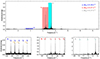 |
Fig. 6. The Fourier transform of the TESS merged Cycle 2 and 4 light curve of the β Cep star HD 192575 (top). The three lower panels are zoomed-in versions of the coloured and labelled frequency ranges, whose averaged splittings are indicated in the upper panel. They consist of a merged quintuplet and quadruplet undergoing an avoided crossing (left), an isolated (possibly incomplete) quintuplet (middle), and a triplet whose prograde mode has the highest amplitude in the entire oscillation spectrum (right). The identifications for the azimuthal order m of these multiplet components are indicated above each peak. The figure was made by Siemen Burssens. |
Fritzewski et al. (2024b) brought the first ensemble asteroseismology for a population of 164 β Cep stars discovered from Gaia DR3 by Gaia Collaboration (2023b). The nature of these pulsators was confirmed from their light curves extracted from the TESS full frame images (FFIs) by Hey & Aerts (2024). We come back to their mode identification in Sect. 8.1, but point out here that this study increased the sample of β Cep stars with a measurement of internal core-to-surface rotation substantially. The level of radial-differential rotation for 48 of these newly discovered pulsators ranges from 1 to 2, except for a few stars that have a value up to 4.
Only a few of the numerous modes active in the fastest rotators among the β Cep stars have been unambiguously identified so far. Much remains to be done on that front, as is the case for the p modes in early-type Be pulsators (such as the CoRoT target HD 49330, Huat et al. 2009). This is not surprising, given the findings of Daszyńska-Daszkiewicz et al. (2002) who studied mode coupling among linear p modes in models of rapidly rotating β Cep stars up to second order in Ω. Their conclusion is essentially that mode identification is only possible if the inclination angle of the rotation axis is well measured, a situation hardly encountered in practice, although modern interferometry gives a promising perspective (Domiciano de Souza et al. 2014; Bouchaud et al. 2020). Lack of mode identification is currently the major challenge to advance asteroseismology of fast-rotating p-mode pulsators of spectral types O to B3, including the pulsating early-type OBe stars whose mode frequencies occur in a similar regime as to those of the β Cep stars (Neiner et al. 2009). We anticipate major progress from asteroseismology of β Cep stars and p-mode Be stars from applying second- or third-order perturbative methods in Ω as in Suárez et al. (2009). Updated modelling from such an approach to all the stars with already identified modes, and even more so from future 2D or 3D stellar evolution models, is an opportunity we come back to at the end of this review.
4.3. Asteroseismic inferences on transport processes from modes of rotating δ Sct stars
We now move on to the case of slowly, moderately, and rapidly rotating δ Sct stars. An extensive catalogue of these pulsators was already available prior to the space era (Rodríguez & Breger 2001). With their masses between roughly 1.5 and 2.5 M⊙, the majority of stars in this class have the most complex internal structures among dwarfs, with a fast-rotating convective core and thin convective outer envelope requiring time-dependent convection theory in a non-adiabatic environment for a proper mode description (Dupret et al. 2005a, 2005b; Antoci et al. 2014).
Bowman (2016) gave an extensive summary of the observational properties of δ Sct stars as evaluated by the end of the nominal Kepler mission, highlighting that their oscillation spectra are characterised by strong amplitude modulation and moderate to fast rotation. This observational behaviour is readily understood in terms of the theory of non-linear mode coupling by Buchler et al. (1997) and Goupil et al. (1998). With the TESS mission ongoing, the class of δ Sct stars keeps increasing with thousands of members (Antoci et al. 2019) with well characterised global properties deduced from the Gaia space data (Murphy et al. 2019). Many of the Keplerδ Sct stars actually turned out to be hybrid γ Dor–δ Sct pulsators experiencing both high-order g modes and low-order p modes (Grigahcène et al. 2010; Uytterhoeven et al. 2011; Bowman et al. 2016; Li et al. 2020b). These are extremely interesting asteroseismic targets as the combination of high-order g modes and low-order p modes offers probing power throughout the entire stellar interior, notably the rotational properties (Audenaert & Tkachenko 2022).
The Ledoux approximation in Eq. (14) is still valid for a small fraction of the δ Sct pulsators. Slow rotation notably occurs among several of the γ Dor–δ Sct hybrid pulsators. The first-order Ledoux approximation was readily applied to the amplitude spectrum of the slow-rotating hybrid pulsator KIC 11145123 by Kurtz et al. (2014). This delivered the first γ Dor–δ Sct star with a determination of internal rotation. This star reveals nearly uniform rotation with a period of about 100 d and a slightly faster surface rotation compared to core rotation. Models with atomic diffusion, including radiative levitation, offer an excellent explanation of the g modes and surface abundances for this hybrid pulsator (Mombarg et al. 2020). Nevertheless, it has been suggested that the star’s ‘weird’ and slow rotation, along with its surface abundances deviating from solar values, may be due to a merger event (Takada-Hidai et al. 2017). While such a scenario should be no surprise (given Fig. 2), another such slowly rotating hybrid γ Dor–δ Sct star, KIC 9244992, has solar-like surface abundances and very similar seismic properties. Its rotation near the surface deduced from p-mode splittings amounts to 66 d, which is slightly slower than the rotation period of 64 d in the near-core region measured from its g-mode splittings (Saio et al. 2015). Both pulsators have a mass of about 1.5 M⊙ and are at an advanced stage of main-sequence evolution, with a central hydrogen mass fraction Xc of about 10%.
Two additional similar cases of slow-rotating hybrid γ Dor–δ Sct pulsators were discovered in the 15.3 d eccentric orbit (e = 0.45) binary KIC 10080943 by Keen et al. (2015), Schmid et al. (2015). Their orbital separation is wide enough to perform asteroseismic modelling assuming the stars to be single yet coeval, as done by Schmid & Aerts (2016). This delivered an age of 1.08 Gyr with a 1.67 M⊙ primary and a 1.60 M⊙ secondary having Xc = 22% and 29%, respectively. The two stars have similar small convective core overshooting and envelope mixing. The primary’s and secondary’s near-core rotation periods are 7.16 d and 11.05 d, respectively. This delivers spin parameters for the detected and identified dipole g modes between 0.20 and 0.26 for the primary, and between 0.14 and 0.24 for the secondary. These values place them well into the super-inertial regime (see Fig. 3). For both stars, the Coriolis force can still be treated perturbatively and the linear modes can be modelled from first-order Ledoux splitting (Schmid & Aerts 2016). The envelope rotation deduced from rotational splitting of p modes resulted in about 7.46 d and 8.20 d for the primary and secondary, respectively. This gives core-to-envelope levels of 0.96 and 1.35, respectively. Thus, the radial-differential rotation of the secondary again reveals a slower core than envelope, just as for KIC 11145123. The centrifugal and tidal forces active in this binary result in only small perturbations, up to 1.7% for the former and below 0.04% for the latter. Thus, the centrifugal force has a stronger influence on the oscillation modes than the tides.
The core-to-envelope rotation rates of these four γ Dor–δ Sct stars were found to be fully in line with angular momentum transport due to internal gravity waves, an interpretation reached from hydrodynamical simulations with appropriate levels of core-to-envelope rotation by Rogers (2015). However, these stars are not representative of the δ Sct class as a whole. The large majority of these pulsators rotate so fast that even second-order perturbation theories in Ω/ω are too limited according to evaluations of Eq. (15) for typical class members. For this reason, a more elaborate third-order perturbation formalism taking into account the Coriolis force and the centrifugal flattening with its coupling with the Coriolis force, was developed by Soufi et al. (1998). For the full expressions of the operators for this third-order perturbative theory in Ω we refer to that paper and the corrections proposed by Karami (2008). To date, this third-order theory has hardly been applied to unravel the internal physics of fast-rotating δ Sct stars. This is due to lack of proper mode identification for a sufficient number of modes, just as for the fast-rotating β Cep and early-type Be pulsators. While Bedding et al. (2020) managed to overcome the hurdle of mode identification for a sample of 60 very young δ Sct stars from regular patterns delivering global parameters of these stars from their large frequency spacing, no rotational splitting was found for this sample. Pressure-mode frequency spacings alone cannot give tight constraints on transport processes to improve the input physics of the models.
Most δ Sct stars do offer the potential to calibrate transport processes. However, this requires more theoretical work on non-linear mode coupling in order to interpret their complex frequency spectra, which include numerous combination frequencies in addition to a variety of frequency structures (Bowman et al. 2016). So far this complexity in the observations has prevented unambiguous mode identifications except partially for a few slow rotators (Zima et al. 2006; Lenz et al. 2008; Chen et al. 2017; Chen & Li 2017; Sun et al. 2023a) or overtone radial pulsators (Murphy et al. 2020; Daszyńska-Daszkiewicz et al. 2023). More than a decade ago, Breger et al. (2012) nicely illustrated that the low-frequency g modes and rotational signals are physically connected to the high-frequency p modes in the fast-rotating hybrid δ Sct–γ Dor pulsator KIC 8054146. This Kepler target is a prototypical case of a non-linearly coupled mode pulsator according to Eq. (2) in the presence of fast rotation (vsini = 300 ± 20 km s−1). Predictions for linear oscillation modes applied to non-rotating evolutionary models following the simplified Eq. (3) as computed by Murphy et al. (2023) are likely insufficient to identify the modes correctly. For hybrid δ Sct–γ Dor stars, non-linear asteroseismology by means of coupled mode equations following Eq. (2), as originally developed by Buchler et al. (1997) and Goupil et al. (1998), offers a way forward, provided that the theoretical formalisms used are generalised to include the Coriolis force to fit the low-frequency g modes as for SPB pulsators (discussed in the next section; Lee 2012, 2022; Van Beeck et al. 2024).
For the fast-rotating pure p-mode pulsators among the δ Sct stars (e.g. Altair; Bouchaud et al. 2020), the challenge is even greater because the mode identification cannot rely on period spacing patterns as for the hybrid pulsators. High-degree p modes also occur among the high-amplitude modes, as Le Dizès et al. (2021) and Rieutord et al. (2023, 2024) have shown from combined MOST and TESS space photometry and high-resolution spectroscopy. High-degree mode asteroseismology at the level of fitting the frequencies of individually identified modes to calibrate transport processes has yet to be developed. For stars such as Altair, this must be done by using future 2D or 3D stellar evolution models, for example those delivered by the ESTER code for stars of higher mass (Rieutord et al. 2016; Mombarg et al. 2023) coupled to 2D or 3D pulsation codes such as TOP (Reese et al. 2006, 2021) or ACOR (Ouazzani et al. 2012, 2015).
Reese et al. (2009a) have shown that the acoustic p modes occurring in spherical stars are turned into island modes for rotationally deformed stars in 2D pulsation computations. As shown by Reese et al. (2009b), these island modes can potentially still be identified in observations, provided that another family of modes, namely chaotic modes, are absent in the frequency spectra. Moreover, Reese et al. (2021) have further shown from 2D adiabatic pulsation computations in the asymptotic regime of high radial order that island modes still show a pseudo large frequency separation. The typical differences between actual numerically computed frequencies and those deduced from asymptotic approximations range from 5% to 12%. This relatively modest frequency difference should in principle safeguard the opportunity to identify island modes from pseudo large frequency separations predicted to occur in deformed p-mode pulsators. This is definitely a promising way forward to advance p-mode asteroseismology of rapidly rotating δ Sct, β Cep, and some of the Be pulsators. Currently these theoretical 2D pulsation predictions for p modes in deformed fast rotators have hardly been turned into practical applications, with the notable exception of Altair in Rieutord et al. (2024).
4.4. Gravito-inertial asteroseismology: High-order g modes in moderate rotators of intermediate mass
Moving to the left in Fig. 3 we end up with dwarfs undergoing slow resonant internal gravity waves with periodicities on the order of days. Gravity-mode asteroseismology was kick-started from data assembled by the CoRoT space telescope (Auvergne et al. 2009), with the discovery of periodic deviations from a constant g-mode period spacing in the B3V star HD 50230 (Degroote et al. 2010). This pulsator’s g modes behave according to the theoretical predictions for non-rotating pulsators made before its discovery in the pedagogical paper by Miglio et al. (2008). Bringing this theory and the CoRoT data together allowed an estimation of the mixing near its convective core. This SPB star is a prototype of the sub-class of slow rotators among g-mode pulsators of intermediate mass, including the SPB star KIC 10526294 whose amplitude spectrum is shown in the bottom part of Fig. 4 and the δ Sct–γ Dor hybrids KIC 11145123 and KIC 9244992 discussed above. The core boundary mixing of such slow-rotating g-mode pulsators have since been deduced in several studies (Wu et al. 2018; Wu & Li 2019; Wu et al. 2020; Mombarg et al. 2020; Pedersen et al. 2021).
However, the majority of B and F g-mode pulsators are moderate to fast rotators whose high-order g-mode periods are of similar order to their rotation period (cf. blue to orange stars indicated in Fig. 4). Most of the identified modes in the 63 well-studied prototypical samples of γ Dor and SPB stars assembled by Aerts et al. (2021) indeed have frequencies in the co-rotating reference frame well below 2Ω. Thus, these modes are in the sub-inertial regime. In this case it is no longer appropriate to treat the Coriolis force perturbatively in Eq. (2), not even for moderate rotators (see Fig. 3). On the other hand, the centrifugal force is less important than the Coriolis force to describe such waves (see Eq. (15)). When the perturbation to the gravitational potential can be ignored (the Cowling approximation), one can make the oscillation equations separable in (r, θ, ϕ) by adopting the TAR for a uniformly rotating star (Lee & Saio 1987; Bildsten et al. 1996; Lee & Saio 1997; Townsend 2003a; Savonije 2005; Mathis 2009). In that case the radial and azimuthal dependencies are the same as for the non-rotating case, while the latitudinal (θ) dependence is governed by Laplace’s tidal equations, whose solutions are written in terms of the Hough functions (Hough 1898) depending only on the spin parameter s = 2Ω/ω. Each eigensolution of the oscillation equations in the TAR is connected to the eigenvalue λl, m, s of the latitudinal equation, instead of l(l + 1) as would occur in the θ-component of the oscillation equations for the non-rotating case. The TAR is valid for modes with frequencies fulfilling ω ≪ Sl, ω ≪ N and ω < 2Ω, and whose ξ(r) is dominantly horizontal at such a level that one can ignore the horizontal component of the rotation vector and assume Ω ≃ (Ωcosθ, 0, 0). This is an excellent approximation for the majority of modes in the γ Dor and SPB stars. A modern public tool to compute oscillation modes of rotating spherical stars in the TAR is available in Townsend et al. (2018). Lee & Baraffe (1995), on the other hand, describe a method for mode calculations in the sub-inertial regime taking the full rotation vector Ω into account, as well as the deformation of the star up to second order in Ω.
The period spacing in the co-rotating frame among low-frequency g modes of the same low degree l and azimuthal order m, while being of consecutive radial order n is denoted as (ΔP)co. It can be approximated by
 (16)
(16)
where r1 and r2 denote the inner and outer position of the mode propagation cavity (Ballot et al. 2012; Bouabid et al. 2013). In the limit of zero rotation, the spin parameter is zero and Eq. (16) reduces to  , where the quantity
 (17)
(17)
has been termed the buoyancy radius of the star (Miglio et al. 2008; Ouazzani et al. 2017). It characterises the size and other properties of the g-mode cavity. For dwarfs the g modes have their dominant probing power just outside the convective core at the deep bottom of the radiative envelope (see Aerts et al. 2021, for illustrations). Since Π0 has the dimension of a time and represents the characteristic period for the g modes of the star, it has also been termed the buoyancy travel time (Aerts 2021).
The mode period spacings observed in an inertial frame (ΔP) can be computed from the mode periods expressed in an inertial frame (Pin) and in the corotating frame (Pco) following the transformation formula
 (18)
(18)
with Prot the rotation period of the star. Equations (16) and (18) offer a powerful observable diagnostic tool to achieve the identification of detected modes from patterns occurring in the amplitude spectra. Such patterns allow us to estimate Ω and Π0 via the involvement of the spin parameter in Eq. (16). This type of asteroseismic inference involving moderate or fast rotation requires long and uninterrupted data strings in order to reach proper precision for the mode periods.
Major efforts to assemble and interpret period spacing patterns for ensembles of gravito-inertial pulsators were undertaken from 4 yr Kepler light curves by Pápics et al. (2014), Pápics et al. (2015), Van Reeth et al. (2015b), Pápics et al. (2017), Szewczuk & Daszyńska-Daszkiewicz (2018), Li et al. (2019), Li et al. (2020b), Szewczuk et al. (2021), and Pedersen et al. (2021). Being more than twice as long as the CoRoT data strings, the TESS light curves for stars in the CVZs also turn out to be suitable to hunt for such patterns (Garcia et al. 2022a, 2022b). We anticipate the discovery of thousands more stars with such oscillation patterns in the future as the TESS light curves become longer. Overall, the observed diagrams of Δ P versus mode periods in the inertial frame of an observer are already available for more than 700 g-mode pulsators, covering stars with masses in the range [1.3, 9.0] M⊙ and all rotation rates from almost zero to critical rotation.
Analysis methods based on the TAR with the aim of deducing the rotation frequency of γ Dor and SPB stars were developed by Van Reeth et al. (2015a) and Ouazzani et al. (2017). The latter authors compared predictions for ΔP from the asymptotic expression in Eq. (16), from numerical computations adopting the TAR, and from full 2D computations with the ACOR code. This led to the important conclusions that ΔP values computed from the TAR for zonal and prograde modes differ only by a few percent from those obtained with ACOR, while retrograde modes may led to differences up to about 10%. The method used to derive Π0 and Ω based on the TAR was applied to a sample of 37 γ Dor stars by Van Reeth et al. (2016), with independent validation of the results by Christophe et al. (2018). A slightly different analysis procedure to obtain Ω was developed by Takata et al. (2020), with overall consistent outcomes for Ω (Ouazzani et al. 2019), but larger diversity (although still consistent) for the somewhat less precise Π0 estimation. Pedersen et al. (2021) tackled the challenging modelling for a sample of 26 SPB stars, where mixing in the core boundary layer and in the envelope is of major importance.
The asteroseismic procedure used to deduce the internal rotation frequency of γ Dor and SPB stars as commonly applied now is illustrated for prograde dipole modes in Fig. 7. The higher the rotation, the steeper the slope in the Δ P versus Pin diagrams for prograde modes. Such modes represent waves travelling along the rotation of the star, and thus their periodic variation re-occurs faster in the line of sight for faster rotation. Hence, the mode periods, and by implication the difference of mode periods for consecutive overtones, decrease. This creates the characteristic downward tilt in the bottom panels of Fig. 7, as predicted theoretically by Bouabid et al. (2013) and put into practice by Van Reeth et al. (2015a, 2016), Ouazzani et al. (2017). Retrograde gravito-inertial modes have the opposite effect and lead to an upward trend characterised by a positive slope (see Van Reeth et al. 2015b, for numerous examples).
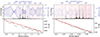 |
Fig. 7. Illustration of the method used to deduce the near-core rotation frequency of a gravito-inertial mode pulsator. The upper panels show a section of the Kepler light curve of the γ Dor star KIC 8375138 (left) and the SPB star KIC 7760680 (right) as derived respectively by Pápics et al. (2015) and Van Reeth et al. (2015b) (blue dots). The amplitude spectra of the 4 yr light curve of these pulsators is overplotted (in black) and reveals a regular pattern of high-order dipole g modes of consecutive radial order (red dashed vertical lines). The lower panels show the measured period spacings of these modes as a function of the mode period (black dots connected by dashed black lines to guide the eye). The red solid line is a linear fit avoiding the trapped modes causing dips in the pattern. The slope of the linear fit is dictated by the internal rotation frequency, Ωrot, in the transition zone between the convective core and the radiative envelope, as deduced by Van Reeth et al. (2015a). The figure was reproduced from Chapter 1 in Van Beeck (2023) by Jordan Van Beeck. |
The detected upward slopes of period spacing patterns in fast rotators laid the foundation for the discovery of toroidal Rossby modes in γ Dor stars by Van Reeth et al. (2016), in additon to the detection of retrograde gravito-inertial modes. It is remarkable that Rossby modes were discovered in many γ Dor stars from Kepler data already in 2016, while they were only detected two years later in the Sun (Löptien et al. 2018), as discussed in Sect. 4.1.1. From their dedicated description of and search for Rossby modes, Saio et al. (2018) found them to occur in the fastest rotators among the γ Dor stars, and in pulsating Be stars with outburst phenomena (Huat et al. 2009; Neiner et al. 2012a; Balona et al. 2015; Rivinius et al. 2016). Although several of the Kepler SPB stars also reveal photometric outbursts, as found by Van Beeck et al. (2021), they have smaller amplitudes than those of the pulsating Be stars and do not necessarily lead to Hα emission in their spectra as is the case for the Be stars. Rossby modes have not yet been found in SPB stars, but the outbursting SPB and pulsating Be stars do share the common property of non-linear mode couplings (Baade et al. 2016; Van Beeck et al. 2021). This detected behaviour and theoretical developments of non-linear asteroseismology (e.g. Lee 2012, 2022; Van Beeck et al. 2024) offer the great future potential to also include mode amplitudes in forward seismic modelling, aside from the frequencies.
A summary of the findings based on 4 yr Kepler light curves of 611 γ Dor stars in terms of stellar properties is available in Li et al. (2020b) and for the internal rotation properties in Fig. 6 of Aerts (2021, not repeated here). The evolutionary context of the g-mode pulsators summarised in that review paper reveal overwhelmingly that dwarfs of intermediate mass have nearly uniform rotation throughout their entire main-sequence phase (see also Van Reeth et al. 2018), irrespective of their mass and current rotation rate. Levels of core-to-surface rotation ratios of γ Dor stars remain below about 10% (Li et al. 2020b), irrespective of the value of the rotation rate itself. The summary of the internal rotation frequencies provided in Aerts (2021) also coupled the angular momentum of intermediate-mass dwarfs to that of evolved low- and intermediate-mass (sub-)giants. This revealed that all these stars transport and lose their angular momentum in such a way that the angular momentum of their helium-burning cores, by the time they are red giants, is in agreement with those of sub-dwarfs and white dwarfs (Aerts et al. 2019).
The ability to estimate Ω(r) and Π0 from (Δ P)in versus Pin diagrams, as illustrated in Fig. 7, along with the envelope rotation from p modes and/or surface rotation from rotational modulation (Van Reeth et al. 2018) laid the foundation for the new sub-field of gravito-inertial asteroseismology for moderate and fast rotators (Aerts et al. 2018). This was applied to samples of F and B pulsators as a way to estimate the level and type of core boundary and the envelope mixing. Calibrating the internal mixing is necessary to properly age-date such stars and to deduce the mass of the helium core they will produce by the time of their core hydrogen exhaustion. Gravito-inertial asteroseismology currently delivers a typical precision of between 5% and 20% for the age and helium core mass at the TAMS (Mombarg et al. 2019, 2021; Pedersen et al. 2021; Pedersen 2022b, 2022a; Fritzewski et al. 2024c). It also provides overwhelming evidence of extra mixing in the near-core region of rotating stars, fully in line with the conclusion drawn from eclipsing binaries (Tkachenko et al. 2020; Johnston 2021). It also shows that the envelope mixing is connected to the internal rotation, but that rotation is not the only physical cause of the element transport (Pedersen et al. 2021; Pedersen 2022b; Mombarg et al. 2023).
Numerically stable tools to compute the eigenvalues of Laplace’s tidal equations are available in Townsend (2020) and make the estimation of the near-core rotation frequency of γ Dor and SPB stars a high-precision observational science. Given that the internal rotation frequency is also accessible from TESS CVZ data, period spacing patterns due to low-degree gravito-inertial modes are within reach for many more pulsators (Garcia et al. 2022a,b), including stars in young open clusters (Fritzewski et al. 2024c; Li et al. 2024b). This opens up the territory of applying gravito-inertial asteroseismology to samples of open clusters with a variety of ages, rotation rates, metallicities, single and binary populations, and merger products with the near-future potential to calibrate the internal structure and angular momentum of young clusters at their birth (see Fig. 1).
Aside from the near-core rotation frequency deduced from gravito-inertial modes in the radiative envelope of intermediate-mass stars, a small fraction of γ Dor stars also offer a powerful observational signal that can be used to derive the rotation rate of the convective core itself. This was first achieved by Ouazzani et al. (2020) from a pertinent characteristic dip in the period spacing pattern of the rapidly rotating γ Dor pulsator KIC 5608334, pointing to mode coupling between a core inertial mode and an envelope gravito-inertial mode in the presence of fast rotation. Saio et al. (2021) subsequently hunted for these inertial core modes, and found the signal in the period spacing diagram for 16 of the 611 γ Dor stars in Li et al. (2020b). These observational findings are readily understood in terms of theoretical expressions for a mode coupling coefficient between inertial core modes and gravito-inertial envelope modes for γ Dor stars derived by Tokuno & Takata (2022). Numerical computations of these coupling coefficients by Aerts & Mathis (2023) from the best characterised γ Dor stars are in agreement with the theory. Although it is pertinent to only a small fraction of γ Dor stars, notably the most rapid rotators, the detection of this mode coupling is of major importance. It opens up the fast-rotating convective cores of F dwarfs for observational scrutiny and confirms that their rotation is almost the same everywhere in their interior, from the core across the entire radiative envelope. Aerts & Mathis (2023) showed that the coupling coefficients for SPB stars are smaller, explaining why such mode coupling is absent for these hotter pulsators.
Another way to probe the rotating convective core was established for a few pulsating late-type Be stars whose modelling is based on their fast rotation and on the observed properties of their stochastically excited low-frequency gravito-inertial modes, without having identifications for the individual modes (Neiner et al. 2012b,a, 2020). These cases are for stars that rotate so rapidly that the Coriolis force cannot be treated either perturbatively or in the TAR. Full pulsation computations in 1D, treating the rotational deformation up to second order in Ω, were done for the Be pulsator HD 49330 by Neiner et al. (2020). The predictions of the oscillation modes were based on the formalism by Lee & Baraffe (1995), with the aim of explaining the observed variability spectrum qualitatively, without fitting individual mode frequencies.
All the observational findings on the internal rotation of gravito-inertial mode pulsators give rise to asteroseismic and evolutionary calibrations of angular momentum from the stellar birth to the evolved phases. Such studies are ongoing for single field stars, and involve the global effect of various rotationally induced processes (Pedersen 2022a; Mombarg et al. 2023) and/or core magnetic dynamo fields (Moyano et al. 2023). The latter are based on the magnetic Tayler instability developed by Fuller et al. (2019) as an improvement on the classical Tayler-Spruit dynamo (see also Takahashi & Langer 2021). Aerts et al. (2021, their Fig. 8) estimated convective and wave Rossby numbers, core boundary stiffness values, and internal magnetic field strengths for a sample of 63 well-characterised gravito-inertial mode pulsators. Assuming a stable dipole field, they predict field strengths in the ranges [104.5, 105.5] G and [105, 106.5] G for SPB and γ Dor stars, respectively. For the γ Dor stars, this is fully in line with the predictions by Cantiello et al. (2016) and Stello et al. (2016) based on dipole mixed mode suppression in about 20% of the Kepler red giants. Direct detections of core magnetic fields from mode splittings or magnetic characteristics in dipole mode period spacing patterns, as recently found in a small fraction of red giants (see Sect. 4.1.3), have not yet been established for gravito-inertial mode pulsators. However, given the numerous recent theoretical formalisms developed to hunt for specific signatures (Prat et al. 2019, 2020; Van Beeck et al. 2020; Dhouib et al. 2022; Rui et al. 2024), it should only be a matter of time for true direct detections to be achieved. For now, an upper limit of the order of 5 ⋅ 105 G was found for the rapidly rotating CoRoT SPB star HD 43317 from asteroseismic modelling by Buysschaert et al. (2018). Lecoanet et al. (2022) confirmed this result by confronting the mode suppression observed in the star with predictions from 3D MHD simulations.
Aside from probing the internal magnetism in or near the core of intermediate-mass pulsators via their gravito-inertial modes, Rossby modes and rotational modulation detected in 162 stars known as ‘hump and spike’ stars gives indirect evidence of magnetic fields in the envelopes of these stars (Henriksen et al. 2023a, 2023b). However, it is still unclear whether the observed variability is due to magnetic spots on the stellar surface triggered by a dynamo field generated in sub-surface layers or is rather caused by overstable convective modes that excite resonant g modes with frequencies equal to the rotation frequency of the convective core (Lee & Saio 2020; Lee 2021, 2022). Further research on the interaction between time-dependent convection, rotation, and magnetism in the nonadiabatic outer envelope is required to fully exploit the detected variability of these fastest rotators.
In conclusion, gravito-inertial asteroseismology of intermediate-mass stars already made internal rotation and will soon make the internal magnetism of moderate and fast rotators an observational science. Exploitation of the detected and identified gravito-inertial modes is applied to hundreds of dwarfs of intermediate mass in the galaxy, with a large potential for asteroseismology of young open clusters of less than a few billion years in age (Fritzewski et al. 2024c; Li et al. 2024b). Such applications of asteroseismology to clusters observed by TESS and PLATO will deliver tight constraints on the angular momentum at stellar birth for various birth masses and metallicity regimes in the not too distant future (see Fig. 1).
5. Adding accurate dynamical masses and radii to increase asteroseismic precision
Asteroseismic modelling of rotating pulsators is a high-dimensional regression problem to solve (Aerts et al. 2018); the aim is to obtain high-precision estimates of the free parameters occurring in the stellar models. Aside from the measured effective temperature and gravity from high-resolution spectroscopy, and the star’s luminosity from Gaia astrometry, it is beneficial to limit the parameter space from additional and preferably model-independent input parameters.
Major advances on this aspect may come from (future) interferometric radii, but this is limited to relatively bright stars. To date, combined interferometry and asteroseismology has mainly been applied to bright slow-rotating low-mass Sun-like pulsators (Cunha et al. 2007; Huber et al. 2012). Applications to fast rotators are scarce and so far can only rely on uninterrupted space photometric light curves of short duration, limiting the identification of sufficient modes (see Rasalhague and Altair analysed by Monnier et al. 2010; Le Dizès et al. 2021; Rieutord et al. 2024, respectively). It is noteworthy that the g modes of the bright hybrid δ Sct–γ Dor pulsator Rasalhague discovered in its MOST data were already correctly interpreted as gravito-inertial modes by Monnier et al. (2010). In our definition, this pulsator is a moderate rotator with a value of  (or
(or  ) for Ω ≃ 1.65 d−1. However, the low frequency resolution of the light curve prevented the detection of clear period spacing patterns and the derivation of ΔP. Moreover, the methodology described in Sect. 4.4 based on the observable diagnostic in Fig. 7 did not yet exist in 2010. It is definitely worthwhile to revisit the few bright fast-rotating pulsators with a good interferometric radius and to hunt for g modes in their space photometry. Moreover, the new SPICA instrument in development at the CHARA array (Mourard et al. 2022) holds great promise to intertwine interferometry and asteroseismology for a large sample of pulsators in the not-too-distant future.
A highly successful and already applied extra constraint on asteroseimic modelling comes from the dynamical masses of detached eclipsing binaries. Binary stars are found in diverse configurations in terms of orbital characteristics and physical properties of their individual components. In this section we focus on the classes of astrometric and eclipsing binaries as ideal test beds to help asteroseismic modelling. The key point is that such objects allow us to infer the masses and radii of the individual components by only relying on the basic laws of binary dynamics. Hence, the masses and radii are model-independent and their precision, and more importantly accuracy, is limited solely by the quality of the observations.
Torres et al. (2010) presented a sample of 95 binary systems (190 stars in total) in a detached configuration, that is, systems where both components are well within their respective Roche equipotential surfaces and do not interact with each other. Their masses and radii are measured to better than 3% accuracy. This sample covers M ∈ [0.2, 27] M⊙ and R ∈ [0.2, 25] R⊙. Serenelli et al. (2021) discussed state-of-the-art methods for the accurate determination of stellar masses and presented a list of 200 benchmark stars, among which binary systems, with relative mass accuracy between [0.3,2]% for the mass range M ∈ [0.1, 16] M⊙. For the sake of brevity, we do not consider every type of binary system in this review, but restrict our analysis to cases with the most precise and accurate determinations of stellar masses and radii. A recent review of eclipsing binaries with pulsating components in the era of space-based mission is provided in Lampens (2021).
Having an accurate mass measurement alone does not enable stellar modelling at high precision due to the multitude of free parameters and the complex correlation patterns involved in the process. However, when combined with asteroseismic modelling, binary observables can break some of the parameter degeneracies. Both components of the binary are coeval and were born with the same initial chemical composition. Moreover, high-precision inferences of the effective temperatures of the stars from spectroscopic methods are possible, thanks to the fact that the components’ surface gravities are known to high accuracy from the dynamical measurements of the stellar masses and radii.
By positioning the binary components in the HRD or Kiel diagram and demanding that the two stars were born together from the same molecular cloud, one can assess whether and how well stellar models are able to predict the dynamical masses and evolutionary paths of both stars. This way, binarity has been exploited in numerous studies in the literature; the studies demonstrate that current stellar models can rarely reproduce the accurately measured properties of individual binary components and that extra physical ingredients are needed to reconcile models and observables. This has led to the need for extra mixing, from relatively small-scale near-core mixing (often simply referred to as convective core overshooting, Schroder et al. 1997; Guinan et al. 2000; Lacy et al. 2008; Torres et al. 2014b; Tkachenko et al. 2014; Meng & Zhang 2014; Claret & Torres 2016, 2017, 2018; Claret & Torres 2019; Higl & Weiss 2017; Pavlovski et al. 2022; Rosu et al. 2020, 2022) to large-scale mixing caused by rotation and/or internal gravity waves (e.g. Ryan & Deliyannis 1995; de Mink et al. 2009; Garland et al. 2017; Pavlovski et al. 2009; Pavlovski & Southworth 2009; Pavlovski et al. 2018, 2023). The need for extra near-core and/or envelope mixing comes from the need of more massive convective cores of the binary components (e.g. Tkachenko et al. 2020; Johnston 2021; Martinet et al. 2021; Rosu et al. 2022). Interactions between magnetic fields, convection, atomic diffusion, and stellar spots have also been invoked to bring the radii of the stars into agreement with model predictions (e.g. Birkby et al. 2012; Torres et al. 2014a; Higl & Weiss 2017; Cruz et al. 2018; Garrido et al. 2019; Morales et al. 2022).
Figure 8 depicts the complementarity among the methods of spectroscopy, asteroseismology, and binarity for stellar modelling. The top row illustrates the type of observations for each method: stellar spectra for atmospheric analysis, periodic brightness variations caused by stellar oscillations for asteroseismic analysis, and periodic dimming of the stellar light and radial velocity variations for binary analysis. The bottom row highlights the gain in precision and accuracy in the modelling as the spectroscopic and asteroseismic methods are combined, at the same time benefiting from the accurate masses of the star from the binary dynamics. If the position of the star in the Teff–log g Kiel diagram is only constrained by its atmospheric parameters inferred from spectroscopy, the typical error box (blue error box in the bottom left panel) is too large to conclude whether the star will follow an evolutionary track of a 7 M⊙ intermediate-mass star with a white dwarf as the end-of-life product, or the one of an 8 M⊙ star that ends its life as a neutron star. The effects of the initial metallicity (red versus black line) and of core boundary mixing (solid versus dashed line) on the evolutionary path of the star are too small to be distinguished with spectroscopic methods alone.
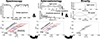 |
Fig. 8. Schematic representation of the complementarity among atmospheric, binary, and asteroseismic analyses. The top row shows observables for each method, while the bottom row highlights the gain in precision and accuracy as the probing power of the different methods is combined. The red curves in the lower left panel represent models for two masses with Z = 0.014, while the black curves have Z = 0.006. The solid lines have no core boundary mixing, while the dotted lines do, increasing the mass of the convective core along the evolutionary path. In the middle lower panel, spectroscopy has allowed us to fix the metallicity, and the red and black curves now differ only in mass, representing evolutionary paths with (dotted lines) or without (solid lines) core boundary mixing. The lower right panel illustrates that asteroseismology further allows us to pinpoint the mass and limit the amount of core boundary mixing. |
Asteroseismology offers unique sensitivity to the physics in the deep stellar interior and is largely complementary to binary and atmospheric analyses in terms of the physical mechanisms these methods probe. Adding asteroseismic constraints delivers the smaller blue box instead of the grey one for a pure spectroscopic solution in the bottom middle panel. This asteroseismic addition improves the modelling substantially as it allows us to eliminate some of the highly improbably solutions, such as those based on the higher- and lower metal content for the 7 M⊙ and 8 M⊙ models, respectively. Moreover, asteroseismic constraints on the amount and functional form of the near-core mixing is often tighter than suggested by the blue error box in the bottom middle panel in Fig. 8, such that the figure represents a pessimistic scenario. Ultimately, the additional model-independent constraint from binary dynamics decreases the error box to a fraction of the pure spectroscopic error box or the combined spectroscopic and asteroseismic error box (blue versus grey boxes in the bottom right panel). This way, one can characterise the physics of the binary pulsator with high accuracy.
Finding binaries for which all three analysis methods depicted in Fig. 8 can be combined is a difficult task, and such studies are therefore still scarce in the literature. The following criteria need to be met simultaneously to do the above-described analysis: (i) the object is an eclipsing or astrometric binary with high-quality photometric or astrometric data; (ii) the object is a spectroscopic double-lined binary such that the radial velocities of both binary components can be measured and their masses can be inferred; (iii) at least one of the components is a pulsator with time series photometry of its brightness variations sufficiently long to achieve high-precision frequencies for sufficient modes; and (iv) at least some of the detected modes can be identified in terms of their (l, m, n). Even if these four conditions are met, it may still be impossible to determine which of the detected oscillation frequencies originates in which star, notably in binaries with components of almost equal mass.
Various slow-rotating low-mass solar-like pulsators in eclipsing or astrometric binaries satisfy all four criteria. Moreover, because the mass and radius of a solar-like pulsator can be inferred directly from its oscillations through scaling relations when the effective temperature of the star is known (Kjeldsen & Bedding 1995), these asteroseismically inferred quantities can be confronted with the model-independent counterparts inferred from binary dynamics (e.g. Gaulme et al. 2013; Appourchaux et al. 2015). While asteroseismic measurements of mass and radius are in a good agreement with the dynamical values for unevolved solar-like pulsators (e.g. White et al. 2017), the asteroseismic masses and radii of red giants are systematically overestimated (e.g. Brogaard et al. 2016; Gaulme et al. 2016; Themeßl et al. 2018; Kallinger et al. 2018; Benbakoura et al. 2021).
Intermediate-mass p-mode δ Sct pulsators in eclipsing binaries constitute another category of objects for applications, although mode identification remains a challenge for such moderate to fast rotators (see Sect. 4.3). For this reason, validation of stellar models with δ Sct pulsators in eclipsing binaries is currently primarily limited to the use of empirical relations between their oscillation properties and mean densities obtained from binary dynamics (e.g. García Hernández et al. 2015, 2017). Because many δ Sct pulsators are found in close Algol-type binary systems (also known as oEA stars; Mkrtichian et al. 2004, 2022) and p-mode oscillations reach their highest amplitudes in the outer layers of stars, oEA stars are often exploited to study binary interactions (see Sect. 6). As for high-mass p-mode pulsators, the discovery of 78 β Cep pulsators in eclipsing binaries by Eze & Handler (2024) in the TESS data is extremely promising to calibrate binary supernova progenitors, of which some may be on their way to becoming gravitational wave emitters.
The group of g-mode pulsators in eclipsing binaries is among the most promising in the context of validation and calibration of stellar models. The main reason lies in the effective probing power of the deep stellar interior facilitated by g modes, in particular the near-core regions (see Sect. 4.4). Binary and asteroseismic analyses become truly complementary in this particular regime and make strategies shown in Fig. 8 optimally suitable. Currently, only a limited number of γ Dor, SPB stars, or white dwarf g-mode pulsators in eclipsing binaries with mode identification are known. Gaulme & Guzik (2019) presented a compilation of 300 pulsating stars in eclipsing binaries observed with Kepler of which about one-third have γ Dor pulsators. Among such pulsators found by Li et al. (2020a) is the remarkable quadruply eclipsing heptuple system KIC 4150611 (Kemp et al. 2024b), whose primary exhibits a long series of prograde dipole gravito-inertial modelled asteroseismically by Kemp et al. (2024a). Further, Southworth & Bowman (2022) and Southworth & Van Reeth (2022) reported the detection of 22 γ Dor, SPB, and β Cep pulsators in eclipsing binaries observed with TESS. For now, however, none of these systems have identified modes.
Sekaran et al. (2020) undertook a systematic search for unevolved g-mode pulsators in eclipsing binaries with period spacing patterns. Among the 93 detected eclipsing systems with a g-mode pulsating component, seven were found to exhibit period spacing patterns. In a follow-up study, Sekaran et al. (2021) investigated one of the detected systems in great detail. This deals with the slow rotator KIC 9850387, whose dynamical parameters are found to be in agreement with the parameters extracted from asteroseismic modelling provided that a high level of internal mixing for the pulsating component is used for its internal structure. The authors proposed that this is a result of intrinsic non-tidal mixing mechanisms. The findings in Sekaran et al. (2021) reinforce the common conclusion in the literature from large samples of single-star pulsators and non-pulsating eclipsing binaries: stellar models require extra internal mixing compared to standard models to achieve a meaninful calibration. Similar studies of moderate to fast rotators with g modes in detached eclipsing binaries are not yet available, given that almost all such objects reveal tidal interactions, as discussed in the next section.
6. Tidal asteroseismology: Interplay between rotation, tides, and oscillations in binaries
The space photometry revolution gave rise to a ‘zoo’ of observed phenomena in Kepler and TESS data caused by tidal interactions in close binaries. Systems with free oscillation modes perturbed by tides, with tidally excited modes, with tidally tilted pulsation axes, with tidal deformation of the mode cavities, and with non-linear mode excitation due to tides have all been found (Guo 2021, for a review). In order to study the effect of linear tides in binaries with rotating components we need to solve Eq. (3), while additional terms (as in Eq. (2)) have to be included for non-linear tides.
Tidally excited oscillations occur at exact multiples of the orbital frequency. They come in various flavours and may be caused by an equilibrium tide in case of a circular orbit and/or dynamical tides in eccentric orbits. An equilibrium tide is a static phenomenon occurring due to the balance between the pressure force and gravity and manifests itself as a geometrical deformation of one star due to the force exerted by the companion. Dynamical tides, on the other hand, cause a periodic acceleration due to  in Eq. (3) as the components revolve around each other in their orbit (see the pedagogical paper by Fuller 2017). Tidal oscillations give rise to slow waves at low frequencies, which naturally occur in close binaries because the orbital, rotation, and g-mode periods are all of similar order and reside in the left part of Fig. 3. On the other hand, self-excited oscillations may get perturbed due to both the equilibrium and dynamical tides, and such deformed oscillations are referred to as tidally perturbed oscillations. They may occur across the whole frequency axis in Fig. 3, including short-period p modes, when tidal forces are significant compared to the other forces at play in the system.
Tidally excited oscillations represent the main mechanism of tidal dissipation in binaries composed of intermediate- or high-mass stars with a convective core and a radiative envelope (Zahn 2013; Alvan et al. 2013; Ogilvie 2014). In a nutshell, the mechanism acts as follows: (i) the tidal potential excites internal gravity waves in the deep stellar interior at the interface of the convective core and the radiative envelope of the star; (ii) these low-frequency travelling waves experience strong damping due to radiative diffusion (Zahn et al. 1997); and (iii) the waves break in the low-density near-surface layers of the star, depositing their energy and angular momentum (Rogers et al. 2013), causing tidal heating and (pseudo-)synchronisation. Such tidal synchronisation is first initiated in the outer layers of the star and gradually proceeds inwards as more waves are being generated through tidal forcing and continue to dissipate. The dissipation is particularly efficient at the critical layers deep inside the star characterised by resonant waves having frequencies equal to the local co-rotation rate (Alvan et al. 2013).
Tidally excited oscillations corresponding to standing waves occur at exact multiples of the orbital frequency. They do not suffer from strong damping, and can therefore be observed in stars. Because the dominant component of the tide-generating potential is a spherical harmonic of l = 2, linear dynamical tides are expected to give rise to quadrupole modes. Some tidally excited oscillations can reach amplitudes exceeding a parametric instability threshold, in which case their mode energy will be transferred to daughter modes through non-linear mode coupling. The observational manifestation of such non-linear mode coupling is the occurrence of pairs or multiplets of daughter modes whose linear combination(s) satisfy resonance conditions (e.g. O’Leary & Burkart 2014; Manzoori 2020; Guo 2020, 2021; Guo et al. 2022). Moreover, some of the tidally excited oscillations can enter into resonance, locking with the orbital frequency of the binary. This happens when the two frequencies evolve in concert. Such orbital resonant mode locking substantially increases the efficiency of tidal dissipation and orbital circularisation (e.g. Witte & Savonije 1999, 2001; Willems et al. 2003; Willems 2003; Burkart et al. 2012; Fuller & Lai 2012; Fuller et al. 2017; Fuller 2017; Zanazzi & Wu 2021; Kołaczek-Szymański & Różański 2023).
It was recently also shown by Li et al. (2020a) and Fuller (2021) that ‘inverse tides’ may occur in close binary systems hosting a g-mode pulsator. In this process, which occurs when the tidally forced mode amplitude approaches the mode’s saturation amplitude, a self-excited oscillation mode transfers (some of) its energy to the binary orbit. This may pump up the orbital eccentricity, create spin-orbit misalignment, and cause asynchronous rotation. This action of tidal dissipation is thus opposite to the standard view and rather pushes the state of the binary away from synchronised circular orbits. Another non-standard effect with respect to tidal theory in a two-body system was presented by Felce & Fuller (2023). They describe how the presence of a tertiary component may trap close binaries into a spin-orbit equilibrium known as a Cassini state. In this case, orbital precession due to the tertiary lies at the origin of the stable spin-orbit configuration. This mechanism has been invoked as an explanation for a minority of close binaries with stars of intermediate mass having extremely slow sub-synchronous rotation. Such a state can be understood by alterations of the spin-orbit misalignment angle and of the internal rotation rate caused by tidal dissipation due to inertial waves (Fuller 2021).
Although the first (ground-based) observations of tidally excited oscillations in close binaries date from two decades ago (Willems & Aerts 2002; Handler et al. 2002; Quaintrell et al. 2003), numerous detections had to await uninterrupted space-based photometric observations and gave rise to the great variety of observed behaviour we know today. Maceroni et al. (2009) reported the detection of tidally excited oscillations in the eccentric binary HD 174884 from CoRoT data. A few years later, Welsh et al. (2011) presented spectacular tidally excited oscillations at the 90th and 91st harmonic of the orbital frequency in HD 187091, also known as KOI-54. The light curve of KOI-54 is characterised by periodic brightness variations near periastron passage caused by geometrical deformation of the star as a response to the instantaneous tidal force. KOI-54 became the prototype of the class of eccentric binaries exhibiting periodic variability in its light curve similar to cardiograms of human heartbeats. These eccentric binaries are therefore also dubbed ‘heartbeat stars’ (Thompson et al. 2012). Just like KOI-54 itself, the majority of heartbeat stars exhibit tidally excited oscillations (e.g. Hambleton et al. 2013, 2016; Kjurkchieva et al. 2016; Pablo et al. 2017; Hambleton et al. 2018; Guo et al. 2017, 2019; Cheng et al. 2020; Kołaczek-Szymański et al. 2021; Jayasinghe et al. 2021; Ou et al. 2021b, 2021a; Wrona et al. 2022; Sharma et al. 2022; Wang et al. 2023). This makes them unique astrophysical laboratories to validate and improve tidal excitation theory (e.g. Burkart et al. 2012; Fuller & Lai 2012; Fuller 2017; O’Leary & Burkart 2014; Guo et al. 2022; Sun et al. 2023b). We refer to Ogilvie (2014) and Guo (2021, and references therein) for comprehensive discussions on the theoretical and observational aspects of tidally excited oscillations in close binaries.
Another distinct group of pulsators in close binary stars is the class of stars with tidally perturbed oscillations, which means that the star’s free oscillations are affected by the presence of a companion. Tidal deformation in a close binary system affects the mode propagation cavities inside the components, as well as the alignment of the pulsation axes. While the effect of the tidal force on the eigenfrequencies of the star has been investigated to a reasonable level of detail with polytropic models (e.g. Saio 1981; Smeyers & Martens 1983; Martens & Smeyers 1986; Reyniers & Smeyers 2003b,a; Smeyers 2005), the consequences of the equilibrium tide on the mode eigenfunctions has been studied only recently (Fuller et al. 2020). While the former effect results in tidal splitting of a self-excited oscillation mode of a given spherical degree l, the Fuller et al. (2020) formalism allows tidal coupling between tidally split multiplets with different angular degree l. The effect of such tidal mode coupling can be three-fold: (i) tidal alignment, where the axis of the oscillations gets aligned with the tidal axis rather than with the rotation axis of the star; (ii) tidal trapping, such that oscillation modes are confined to regions corresponding to the tidal pole or equator; and (iii) tidal amplification, increasing flux perturbations in the tidal polar regions due to the propagation of acoustic waves close to the stellar surface.
Observationally, tidally perturbed oscillations (which include both tidally split and trapped oscillations) manifest themselves as (a series of) modes that are offset from their adjacent orbital harmonics and are (quasi-)equidistantly spaced with the orbital frequency of the star (e.g. Balona 2018; Lee 2021; Steindl et al. 2021; Van Reeth et al. 2022; Jennings et al. 2024). Some of the class members exhibit readily interpretable observed frequency patterns due to one of the above theoretical scenarios (e.g. some of the tidally tilted pulsators; Handler et al. 2020; Kurtz et al. 2020; Rappaport et al. 2021; Jayaraman et al. 2022; Kahraman Aliçavuş et al. 2022; Aliçavuş et al. 2023). However, others show patterns that are either very complex or too sparse to interpret (e.g. Bowman et al. 2019; Southworth et al. 2020; Jerzykiewicz et al. 2020; Southworth 2021; Southworth et al. 2021; Kálmán et al. 2022; Van Reeth et al. 2023; Johnston et al. 2023; Kálmán et al. 2023). Furthermore, in the specific case of eclipsing binaries, the geometrical effect of eclipse mapping due to particular obscuration of the visible disk of the pulsator by its companion (Reed et al. 2001, 2005) causes extra orbital phase-dependent variability of the mode amplitudes. Depending on the mode geometry, on the misalignment of the axis with respect to the rotation axis of the star, and on the geometry of the eclipse, the amplitude modulation can manifest itself as a complex frequency pattern in the Fourier transform of the light curve, as in the case of U Gru (Johnston et al. 2023).
Recent advances in asteroseismology of (close) binary stars can hardly be overestimated, both from the theoretical and observational point of view. Major efforts are undertaken to develop a general enough tidal oscillation theory as a pertinent need to explain the zoo of observed phenomena resulting from the interplay between tides and oscillations brought by the high-precision space photometry. The novel theories mentioned above are powerful in terms of the effects due to the tidal, Lorentz, Coriolis, and centrifugal forces acting on a rotating pulsating star in a close binary or triple system, taking into account misalignments between the axes of apsides and rotation (Fuller et al. 2020; Fuller 2021; Sun et al. 2023b).
The classes of observed stars exhibiting tidally excited and tidally perturbed oscillations open up the new window of tidal asteroseismology, irrespective of the rotation rate, from ultra-slow to very fast. Progress in the forward modelling of the internal physical properties from carefully identified modes is the next extremely challenging step, given the numerous orbital parameters involved, as well as the numerical aspects involved in modal decompositions and the computation of damping coefficients, and the complex physical phenomenon of pseudo-synchronisation (Townsend & Sun 2023). While we are still waiting for a concerted plan of attack for tidal asteroseismic modelling, applications to large samples of close binaries are the best way to understand and calibrate tidal dissipation and close binary evolution. Achieving this would be a major step ahead as input for proper binary population synthesis and gravitational-wave progenitor modelling (see Fig. 1). The modern public tool to model stellar tides developed by Sun et al. (2023b) is highly relevant in this context.
7. The special cases of sub-dwarf and merger seismology
Sub-dwarfs play a special role in terms of close binarity as their bare existence demands binary interaction at evolved stages of stellar evolution, including mergers (Han et al. 2003). Either they occur in a binary or they are single sub-dwarfs as the result of a merger (Heber 2009). Just as is the case for white dwarfs, the asteroseismology of sub-dwarfs has advanced appreciably thanks to short-cadence (1 min, 2 min, or 20 sec) light curves assembled with Kepler, K2, and TESS (Hermes et al. 2017; Bell et al. 2019; Reed et al. 2021; Uzundag et al. 2021; Córsico et al. 2022; Uzundag et al. 2022; Romero et al. 2022), including post-merger sub-dwarfs (Vos et al. 2021). Asteroseismic probing of almost all sub-dwarfs and all white dwarfs is done from the modelling of their identified g modes via period spacing patterns and/or rotationally split triplets and quintuplets, where the Coriolis and tidal forces can be treated as a small perturbation for the computation of the modes because the periods of all detected modes (minutes to hours) are much shorter than the rotation or orbital periods (days).
A review of white dwarf asteroseismology was presented by Córsico et al. (2019), but no such comprehensive summary is available for sub-dwarfs. This is far beyond the scope of this paper, and hence we just highlight some recent findings for sub-dwarf binaries. Two major conclusions connected with transport processes can be drawn from published sub-dwarf asteroseismology:
-
The angular momentum of the convective core of red giants and of sub-dwarfs is in agreement with the angular momentum of white dwarfs (Aerts et al. 2019);
-
Sub-dwarfs and white dwarfs have respectively more massive helium and carbon–oxygen cores compared to those predicted by standard stellar evolution models without extra mixing beyond the Schwarzschild boundary. Hence, core boundary mixing is prominent throughout the evolution of low- and intermediate-mass stars (Van Grootel et al. 2010a,b; Charpinet et al. 2011; Hermes et al. 2017; Charpinet et al. 2019a,b; Giammichele et al. 2018; Uzundag et al. 2021; Giammichele et al. 2022, where the latter review paper places both types of compact pulsators and the properties of their carbon-oxygen cores into an evolutionary context).
Future progress in the calibration of close binary evolution at evolved phases can come from several aspects. Importantly, many of the modes of sub-dwarfs and white dwarfs exhibit amplitude and frequency modulations on timescales of weeks to months, pointing to non-linear resonant mode interactions. The exploitation of such interactions is easier than for the rapidly rotating SPB and γ Dor stars discussed in Sect. 4.4, and is therefore somewhat more advanced (Zong et al. 2016a,b). However, much remains to be done in the development and application of non-linear asteroseismology, also for the compact pulsators. The recent finding of radial-differential rotation between the core and surface at the level of about 1.2 in the sub-dwarf EPIC 220422705 by Ma et al. (2022) is an important step towards the future modelling of its non-linear modes.
As for the calibration of binary evolution theory, several recent key findings were delivered by asteroseismology. Importantly, short-period sub-dwarf–M dwarf binaries are not necessarily synchronised. A key laboratory for further study is TIC 137608661, whose core rotates slower than its surface, with a period of 4.6 d deduced from g-mode asteroseismology. This core rotation period is much longer than the short orbital period of only about 0.3 d. The asteroseismic study of this sub-dwarf binary was placed into the context of sub-dwarf rotation and binary properties by Silvotti et al. (2022). Their Table 4 and Fig. 16 suggests close to rigid rotation for most of the other sub-dwarfs in short-period binaries with either an M-dwarf or a white dwarf companion. Another striking result comes from the tidally tilted oscillations (see Fuller et al. 2020, as discussed in the previous section) of the binary sub-dwarf HD 265435 discovered and analysed by Jayaraman et al. (2022). Its white dwarf companion revolves around it in only 1.65 h. The sub-dwarf was found to be near or just beyond the end of its central helium burning, and hence this object is a Type Ia supernova progenitor. Most, but not all, of the sub-dwarf’s oscillations have frequencies that are exact multiples of the orbital frequency. This star was diagnosed with acoustic modes having periods of around 250 s. To date, these tidally tilted oscillations have been modelled, while the Coriolis and centrifugal forces have been ignored. However, the tidal distortion for a binary with such a tight orbit shifts the mode frequencies appreciably compared to the case of a spherical star as the authors have assumed. Future measurements of the internal and surface rotation for more short-period binaries are key to guide theories of tidal synchronisation.
Backtracking to earlier phases, Deheuvels et al. (2022), Li et al. (2022c), and Rui & Fuller (2024) used asteroseismology of red clump red giants to identify groups of stripped stars due to binary interactions. One group comprises several underluminous red giants with smaller than usual helium burning cores, which are interpreted as resulting from heavy mass loss due to envelope stripping by a companion while they ascended the red giant branch. Another group consists of tens of red giants whose ages would exceed the age of the Universe if interpreted from single-star evolution with no or nominal mass loss on the red giant branch. However, another mechanism leads to core-helium burning red giants with higher than usual luminosity as a result of the consumption of a white dwarf during the earlier main-sequence phase. The small sample sizes of these observed anomalous groups are consistent with binary fractions as in Fig. 2. Coupling the properties of these red giants to models of post-mass-transfer binary systems will be invaluable to calibrate binary evolution theories of low- to intermediate-mass stars.
Moving on to the even earlier phases and to more massive stars, Fig. 2 and binary evolution calculations by Schneider et al. (2020) tell us that 20% of OB stars come into contact with their companion. Hence, a large population of binary mergers must exist, either formed from collision or from more gentle coalescence (Schneider et al. 2019). The properties of such mergers are highly uncertain and searching for such products is difficult. Asteroseismology could play a major role here, both in terms of establishing a proper calibration for the statistics of the sample of high-mass mergers and of probing their internal structure. This would allow us to check whether mergers indeed have a strong large-scale magnetic field, as the MHD simulations by Schneider et al. (2019) predict. The first calculations of seismic diagnostics for stellar mergers were compared with those of single blue supergiants in the hydrogen shell burning phase (called the Hertzsprung gap (HG) in the HRD), of main-sequence stars with an exceptionally high level of core overshooting, and of evolved single blue giants undergoing a blue loop during their core-helium burning by Bellinger et al. (2024). These authors computed grids of non-rotating equilibrium models and their oscillation frequencies for these four different populations, considering the mass range [10, 20] M⊙. This theoretical study shows that asteroseismology in principle offers the potential to distinguish among these four cases from the large frequency separation of identified p modes and the average period spacing of identified g modes. A major point to be improved is to include internal rotation in such models.
To illustrate the potential of ‘merger seismology’ (a term suggested by Dr. Fabian Schneider from the Heidelberg Institute for Theoretical Studies) from a practical point of view, we show in Fig. 9 the predicted seismic g-mode period spacings of a merger product in the HG and compare them to those of a single blue giant residing in the same part of the HRD, following the study by Henneco et al. (2024). It can be seen that the period spacing values of these two models are clearly different in the sense that the average period spacing of the merger product is lower than that of a model resulting from nominal single-star evolution. This is in agreement with the results found by Bellinger et al. (2024). Moreover, the oscillations of the merger shown in Fig. 9 lead to different mode periodicities and dip structures in the period spacing patterns compared with those of the single HG star. The shorter mode periods and the sharper dips at high radial order for the merger are due to particular structures in its Brunt-Väisälä frequency, originating from the chemical properties near its core reflected in its μ-gradient. The occurrence or absence of intermediate convection zones, often caused by semi-convection, also plays a role. The profile of N(r) for the two models with similar positions in the HRD are markedly different, resulting in different mode trapping and mode coupling according to the occurrence of various mode cavities. Signatures such as those in Fig. 9, when computed for a representative population of mergers with proper inclusion of internal rotation, will provide a powerful tool to search for merger products in a machine-learning context when applied to Kepler and TESS light curves. Once found, modelling the morphology of the period spacing pattern(s) would allow us to assess the profiles of the internal chemical composition, rotation, and magnetic field of mergers.
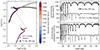 |
Fig. 9. Illustration of the potential of merger seismology. The left panel shows two evolutionary tracks for non-rotating stellar models, colour-coded by the value of the buoyancy travel time Π0 defined in Eq. (17). The black dot indicates the position of a single star born with 9.2 M⊙ at the ZAMS. The grey square is the position of a 6.0 M⊙ primary at the ZAMS, accompanied by a 4.5 M⊙ close companion. The binary components merge via a Case B mass transfer following the description by Schneider et al. (2021). This happens when the primary evolves beyond the TAMS, as indicated by the dotted line. The single star and merger product reside in a similar position while crossing the Hertzsprung gap (HG). The right panels show the predicted period spacing patterns for dipole (upper panel) and quadrupole (lower panel) high-order g modes of the single star undergoing hydrogen shell burning (black circles) and of the merger product (grey squares), at the evolutionary stage indicated by the green cross in the left panel. At this time the merger burns helium in its convective core and has a convective region due to hydrogen shell burning, while the inner structure of the single star is fully radiative, including its shell burning region. The figure was produced by Jan Henneco, from models in Henneco et al. (2024). |
TESS is currently monitoring about 1500 massive OB dwarfs, giants, and supergiants across the sky at a cadence of 2 min. Figure 2 makes it clear that dedicated searches for signals of merger products among these stars based on the predictions in Fig. 9 offer an interesting route for massive star asteroseismology. Future searches in the TESS data are highly relevant to calibrate populations of gravitational wave progenitors seismically because mergers should also occur in what were originally double, triple, or multiple systems in general. The discovery of 78 β Cep stars in eclipsing binaries, including 59 new pulsators, by Eze & Handler (2024) offers a fantastic new data set to apply the principles in Fig. 8 and to predict how many of these targets will evolve into a merger before or after the supernova explosion(s) that will be happening during their future evolution. Discovering mergers from seismology, unravelling their internal structure, and comparing it to the structure of massive SPB or β Cep detached or semi-detached binaries offers a great way to calibrate tidal dissipation and close binary evolution. It would also provide an elegant and independent way to evaluate the measured mass distribution of the black hole and neutron star mergers that lead to gravitational wave signals (see Fig. 1).
8. Onward to a bright future for asteroseismology, for slow and fast rotators
The TESS mission keeps on going, and currently provides ever longer time series photometry covering many years (albeit with interruptions of a year for each of its covered sectors). Moreover, the launch of the PLATO mission is on the horizon (late 2026, at the time of writing). With its core programme focused on exoplanet host candidates and its open Guest Observer programme, it will cover slow to fast rotators in all evolutionary phases, from single stars through binaries and multiples to clusters of various ages and metallicities (Rauer et al. 2024). Even without the additional candidate space missions based on a similar principle of high-cadence high-precision uninterrupted space photometry, such as the High-precision AsteroseismologY of DeNse stellar fields mission (HAYDN, Miglio et al. 2021) and the mission ExtraTerrestrial: To Find the First Earth 2.0 (ET, Ge et al. 2022), TESS and PLATO guarantee a bright future for asteroseismology for many years to come. A wealth of suitable light curves covering many years with high duty cycle will become available for millions of stars. These data feed the fountain of opportunities shown in Fig. 1 and will allow us to push asteroseismology to high-mass stars (unavoidably in close binary systems; see Fig. 2), covering from early to evolved evolutionary phases, with some on their way to becoming gravitational wave sources.
As we have tried to emphasise in this review, asteroseismology based on numerous low-frequency modes in moderate to fast rotators requires long and uninterrupted data strings to reach sufficient frequency precision and to unravel long and complex beating patterns (see Fig. 7). Even the 4 yr uninterrupted Kepler light curves are insufficient to resolve some of the individual modes of γ Dor, SPB, and Be pulsators. Years-long time strings are also necessary to detect and model the internal rotation and magnetic field profiles inside stars.
8.1. Pushing Gaia beyond its limits to assist in the asteroseismology of intermediate- and high-mass stars
The Gaia space mission of the European Space Agency (Gaia Collaboration 2016) was not designed to do asteroseismology. High sampling rates and continuous monitoring with duty cycles above 90% are required to perform asteroseismology. This is needed to push the Nyquist frequency of the light curves to high enough values, and to detect and identify a sufficient number of oscillation modes. Gaia cannot deliver that. In particular it cannot offer mode detections for amplitudes below the millimagnitude range as required to detect solar-like oscillations. Nevertheless, Gaia has a significant role to play, particularly for the asteroseismology of moderate and fast rotators.
All asteroseismic modelling efforts currently benefit from Gaia’s data, notably the high-precision parallaxes (Gaia Collaboration 2018), leading to luminosities that guide the computation of grids of equilibrium models required for the modelling. For slow-rotating low-mass stars, the Gaia effective temperatures additionally lead to fairly precise radius estimates, which can be confronted with the asteroseismic values. Conversely, combined asteroseismic radii and Gaia effective temperatures lead to asteroseismic distance estimates of remarkable precision, up to distances of kiloparsecs (Huber et al. 2017; Davies et al. 2017).
The continued improvement of the Gaia, Kepler and TESS data reductions provide excellent means for more accurate instrument calibrations, with ever better future capacity for large and homogeneous population studies. Along with the Gaia distances and proper motions, precise asteroseismic ages are particularly valuable for galactic archaeology studies (see Fig. 1).
We also point to additional roles that Gaia can play by pushing beyond the nominal use of its data. The three light curves made available in Gaia’s Data Release 3 (DR3) in the G, RP, and BP photometric bands delivered millions of new variable stars (Eyer et al. 2023), among which thousands of candidates with non-radial oscillations having amplitudes above a few mmag (Gaia Collaboration 2023b). Figure 10 shows the position of more than 100 000 new (non-)radial pulsators in the upper HRD discovered from Gaia DR3. This figure includes a comparison with the positions of four instability strips where non-radial modes are expected to be excited based on one particular choice of input physics for each of the β Cep, SPB, δ Sct, and γ Dor pulsator classes. We know from asteroseismology that such comparisons with one strip per class based on only one choice of input physics is too limited, in view of the large variety of internal rotation rates and mixing levels in the interior of single and binary stars in that part of the HRD (e.g. Moravveji et al. 2015, 2016; Szewczuk & Daszyńska-Daszkiewicz 2018; Wu & Li 2019; Wu et al. 2020; Mombarg et al. 2020; Pedersen et al. 2021; Pedersen 2022b; Szewczuk et al. 2022). This can explain why many stars occur outside of the particular strips chosen to illustrate the comparison in Fig. 10. A similar conclusion was reached from the summary by Balona (2023) based on assembled space photometry over the past decade. Proper comparisons between the observed and theoretically predicted position in the HRD can help to improve the input physics and delineate free parameters used in stellar models. This is a question of various choices for opacity tables and chemical mixtures, for the mixing length parameter of (time-dependent) convection calculations, and for parameters used to describe transport processes caused by rotation, magnetic fields, and atomic diffusion, including radiative levitation (Townsend 2005; Dupret et al. 2005a,b,c; Moravveji 2016; Szewczuk & Daszyńska-Daszkiewicz 2017; Rehm et al. 2024, to list just a few papers treating some of these phenomena).
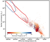 |
Fig. 10. HRD showing the position of more than 100 000 candidate (non-)radial oscillators discovered from the Gaia DR3 G-band light curves, colour-coded according to their dominant frequency. The thick lines indicate the borders of four instability strips for solar metallicity computed by Burssens et al. (2020) and Dupret et al. (2005a), enclosing areas where theoretically predicted g modes (solid red lines) and p modes (dashed blue lines) are expected for the chosen input physics of the models. The figure was produced by Dr. Joris De Ridder from data in Gaia Collaboration (2023b). |
The more than 15 000 new candidate g-mode pulsators discovered from Gaia DR3 shown in Fig. 10 have global properties fully in line with the Kepler pulsators in these classes (Aerts et al. 2023), including their chemical composition (Gebruers et al. 2021; de Laverny et al. 2024). This offers great potential for ‘industrialised’ ensemble asteroseismology of thousands of intermediate- and high-mass stars. The requirement to embark upon this is that sufficient non-radial modes can be identified per star, for example from dedicated space photometry by Kepler, TESS, or PLATO, in addition to the identification of their dominant mode(s) discovered in the Gaia photometry. For now, identifications of a sufficient number of modes are only available for about 700 moderate and fast rotators observed by Kepler (Pedersen et al. 2019; Antoci et al. 2019; Cunha et al. 2019; Burssens et al. 2020; Skarka et al. 2022; Garcia et al. 2022a).
Hey & Aerts (2024) provided a path forward to extend this Kepler sample by scrutinising the light curves extracted from TESS FFIs for the 60 000 candidate pulsators in Fig. 10 with such data available. They confirmed the large majority of these 60 000 stars to be multi-periodic non-radial pulsators, and found the same dominant frequency in the TESS FFI light curves as found in the sparse Gaia DR3 light curves, highlighting Gaia’s capabilities to detect good asteroseismology targets.
Mombarg et al. (2024a) followed up on Hey & Aerts (2024) and determined the (convective core) masses, radii, and evolutionary stages for more than 14 000 g-mode pulsators from their Gaia DR3 data, after having confirmed their dominant oscillation mode from TESS FFI data. To achieve this they relied on grids of models calibrated by Kepler asteroseismology in terms of element and angular momentum transport computed by Mombarg et al. (2024b). These Gaia-based results deliver many non-radial pulsators with a mass between 2 and 3 M⊙, while none are expected from current excitation theory. This discrepancy between theory and observations will trigger further research, given the poorly known uncertainties of the Gaia DR3 observables of hot stars. Moreover, following Fig. 2, a large fraction of the stars inside and between the instability strips shown in Fig. 10 could be as-yet-unknown binaries or mergers. Their deduced luminosity and effective temperature may thus be particularly prone to systematic uncertainty as the Gaia processing ignored their potential (former) multiplicity.
Pushing even more beyond the limits, we can now fully integrate the knowledge from Gaia’s three-band and Kepler’s and/or TESS’s (or in the future PLATO’s) single-band light curves to improve asteroseismic modelling. Such a synergistic integration of data is illustrated in Fig. 11, which compares the amplitudes of the dominant dipole prograde mode in the Gaia BP and KeplerKp bands for 309 γ Dor stars. Theory predicts the amplitudes of dipole modes in γ Dor pulsators to be higher at the BP than at the Kp wavelengths (Aerts et al. 2004). This is in agreement with the results for g-mode pulsators shown in the right panel in Fig. 11. This panel shows the amplitude ratios of the 23 γ Dor stars among the sample of 309, for which a harmonic fit with the dominant Kepler frequency explains at least 50% of the overall variance in the Gaia BP and RP time series. Measured amplitudes depend on the inclination angle of the star’s symmetry axis of the oscillations with respect to the line of sight and on the position of the surface nodal lines. However, for slow rotators, both dependencies drop out of the theoretical expression of amplitude ratios with respect to a reference wavelength (see Chapter 6, Aerts et al. 2010, for details). Theoretical expressions for the ratios in the approximation of the TAR are also available (Townsend 2003b). This implies that measured amplitude ratios contain integrated astrophysical information about the properties of the stellar atmosphere, notably its aspect-angle dependent effective temperature, gravity, and limb darkening, all of which occur in the theoretical expressions of the ratios. While this was used as an attempt to identify mode degrees from models with fixed input physics prior to space asteroseismology, Gaia now also offers the reverse for stars whose frequencies and amplitudes of already identified modes are detected in the Gaia BP and RP photometry.
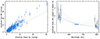 |
Fig. 11. Comparison between the amplitudes of the dominant g-mode frequency in the Gaia BP and KeplerKp bands, whose maxima in the response functions occur at 517 nm and 640 nm, respectively. The left panel shows the results for the 309 γ Dor stars from Li et al. (2020b) with time series photometry available in the public domain of both surveys. The frequency deduced from the Kepler data was imposed on the Gaia DR3 data to produce this plot. The right panel shows the Gaia BP and RP (response curve peaking at 783 nm) amplitude ratios with respect to the one in Kp, plotted as a function of wavelength for the 23 γ Dor stars in the sample with an identified dominant prograde dipole mode explaining more than 50% of the total variance in the Gaia BP and RP light curves. The three values for each star are connected by a dotted line to guide the eye. The results for each star have been shifted slightly in wavelength for visibility reasons. The errors for Kp are smaller than the symbol size. |
In addition, Fritzewski et al. (2024b) showed that the Gaia BP and RP photometry may lead to the identification of the degree of low-order modes in β Cep stars. They designed a novel probabilistic identification method and applied it to the dominant mode detected consistently in the Gaia BP, RP, and TESS data of 164 β Cep stars included in Fig. 10, among which 121 new pulsators discovered from Gaia. This mode identification and the detection of rotationally split modes in the TESS FFI data led to the first forward modelling of a population of high-mass pulsators, resulting in masses between 9 M⊙ and about 20 M⊙ for these 164 stars. For 48 of them, limits on the core-to-surface rotation ratios were derived from the combined Gaia and TESS data; most of these stars have values below 2, but a few objects reveal a ratio up to ∼4. Such internal rotation estimates were only available for five class members before Gaia DR3.
These examples illustrate that Gaia already has an important role to play in asteroseismic modelling of intermediate- and high-mass pulsators. Much more is to come in the near future. Since the 23 γ Dor stars in Fig. 11 have similar metallicity and the same mode identification in terms of (l, m), future exploitation of their amplitude ratios may reveal their atmospheric properties, which are currently unknown. This may even help us to find optimal stars with a variety of surface phenomena, such as spots and lattitudinal-differential rotation, for calibration purposes of new high-resolution spectrographs to study exoplanet hosts (see Fig. 1). Figure 11 shows that the uncertainties in the Gaia BP and RP amplitude ratios are currently still too large to exploit this potential, but they should decrease appreciably for the longer light curves to be expected from Gaia Data Releases 4 (2026) and 5. These will occur at the time when the PLATO mission should be operational. PLATO itself offers two-colour photometry from its two fast cameras, and is even more suited to push this research beyond current instrument barriers than Kepler or TESS combined with Gaia. In addition, ground-based survey facilities with the capacity to deliver multi-colour photometry at the millimagnitude level are operational or will become operational soon, such as BlackGEM (Groot et al. 2024) and the Vera Rubin Observatory (formerly known as the Large Synoptic Survey Telescope (LSST), Di Criscienzo et al. 2023). The basics of modelling tools used to interpret the amplitude ratios in moderate and fast rotators had already been developed long before the era of space asteroseismology (e.g. Daszyńska-Daszkiewicz et al. 2002; Townsend 2003b). Now, about two decades later, modern tools such as those designed by Fritzewski et al. (2024b) can be applied massively from combined Gaia, Kepler, TESS, PLATO, BlackGEM, and Rubin multi-colour survey photometry for all the pulsators with proper identification of their mode(s). Exploitation of the amplitude ratios in terms of internal and atmosphere physics from modern multi-colour photometry should be within reach for modes with amplitudes of several mmag.
8.2. The need for better theory and modelling tools
Optimal exploitation of the wealth of available and future observations of stellar oscillations requires concerted efforts to develop better theory. This need is particularly prominent for the theory and modelling of non-radial oscillations in fast-rotating single stars and close binaries. In order to treat moderate and fast rotators up to the level of the precision of modern data, we must go beyond the current modelling tools and develop non-linear pulsation theory involving mode coupling and non-linear inversion tools (Vanlaer et al. 2023; Farrell et al. 2024). Ample detections of amplitude modulation (e.g. Bowman 2016) and non-linear mode coupling (e.g. Huat et al. 2009; Breger et al. 2012; Kurtz et al. 2015; Baade et al. 2016; Van Beeck et al. 2021) in fast rotators are available, while most asteroseismic modelling currently only relies on measured frequencies assuming linear and uncoupled modes. Non-linear asteroseismology would allow us to exploit mode amplitudes from coupled mode equations. Following the initial pioneering steps in non-linear space asteroseismology for slow-rotating evolved sub-dwarfs and white dwarfs by Zong et al. (2016a,b), similar applications to moderate and fast rotators along the main sequence have yet to be tried out. This can be done by extending the principles laid out by Buchler et al. (1997), Goupil et al. (1998), Mourabit & Weinberg (2023), among others, by means of a proper treatment of the rotation. Lee (2012, 2022) and Van Beeck et al. (2024) include the Coriolis force for modes in the sub-inertial (see Fig. 3), providing enhanced theory to model the numerous gravito-inertial non-linear pulsators with identified multi-mode couplings. Asteroseismic modelling based on these non-linear formalisms would allow us to scrutinise transport processes from early phases of evolution onwards. This would constitute a critical step ahead because the effects of angular momentum transport and chemical mixing are cumulative, and hence have major implications for the entire life of the star, from birth to death.
Finally, moderate and fast rotators require attention at an even more fundamental level than developing and applying non-linear asteroseismology. If we truly want to maximise the exploitation of the asteroseismic data of such pulsators, we must abandon the premise that stars can be approximated as spheres, both at the level of the stellar structure equations and in solving the oscillation equations to compute the modes. Rotating stars are oblate spheroids, requiring at least 2D (for rotating single stars) and optimally 3D (for magnetic spheroids and/or binary systems) treatments. Realistic evolution models including the chemical evolution of stars are being constructed (Deupree 1990, 1995; Rieutord et al. 2016; Mombarg et al. 2023) and so are numerical computations of their oscillation modes (Ouazzani et al. 2015; Reese et al. 2021). Major long-term mathematical and computational efforts to achieve this in a systematic approach are on the horizon1 and offer a fantastic opportunity to bridge the fields of asteroseismology, close binary evolution, binary population synthesis, and gravitational wave astrophysics, as highlighted in the fountain in Fig. 1.
Key points of the review
Takeaway messages from the asteroseismology of fast rotators in the literature include:
-
Asteroseismology of stars rotating up to 70% of their critical Keplerian rotation rate is a mature field of research, delivering their mass, radius, core mass, and core radius with a precision of a few percent for the best cases.
-
About 80% of the detected g-mode oscillations in intermediate-mass dwarfs are prograde dipole gravito-inertial modes. These modes deliver the near-core rotation frequency to better than 5% accuracy. Values range from zero to 30 μHz.
-
For a small fraction of the fastest rotators in the mass range [1.3, 1.9] M⊙, inertial modes in the convective core couple to gravito-inertial modes in the envelope, offering a direct measurement of the rotating core properties.
-
Single intermediate-mass dwarfs have modest radial-differential rotation, with their core and surface rotation frequencies differing by less than 10%. The asteroseismic results imply rapid transport of angular momentum from the core to the surface during the main sequence.
-
About 15% of the fast-rotating dwarfs in the mass range [1.3, 1.9] M⊙, as well as some of the outbursting Be pulsators, reveal global Rossby modes.
-
Non-linear resonant mode coupling is omnipresent in rotating intermediate-mass pulsators and in their sub-dwarf and white dwarf successors. This offers a golden opportunity to exploit mode amplitudes in addition to frequencies.
-
The fastest rotating B and Be pulsators in the mass range [3, 9] M⊙ show outbursts in their photometric light curves, often accompanied by non-linear mode coupling.
-
Asteroseismic core-to-surface rotation ratios have been determined for about 50 high-mass dwarfs in the mass range [8, 20] M⊙, revealing values below 2 for most of them, but a value up to 5 for a few stars.
-
The cumulative effect of the measured near-core mixing in dwarfs with a convective core extends the duration of their main sequence and induces large spreads at the turnoff. This mixing impacts all phases of evolution, notably age-dating and chemical yield production. Up to twice as much helium can be produced by the time of the turnoff compared to the case without any near-core mixing.
-
Evidence of enhanced internal mixing during the core-helium burning phase is uncovered from asteroseismology of white dwarfs and sub-dwarfs, but has yet to be calibrated with high precision for large samples.
-
Measured vertical diffusive envelope mixing levels in single intermediate- and high-mass dwarfs range from 10 cm2 s−1 to 107 cm2 s−1. The near-core and envelope mixing profiles are diverse and change over time.
-
Internal magnetic fields are detected in a fraction of pulsators across the entire evolution and mass ranges accessible by asteroseismology, revealing field strengths between 104 G and about 106 G.
-
Model-independent dynamical masses of detached eclipsing binaries offer tight constraints on asteroseismic modelling, confirming that stellar models require near-core boundary mixing to bring (core) masses from theory and observations into agreement.
-
Tidally excited, tidally perturbed, and tidally tilted oscillations occur across a wide range of binaries, including supernova progenitors and members of young open clusters. This makes asteroseismic calibration of tidal dissipation processes and of close binary evolution models possible, including binaries en route to gravitational wave emission.
Acknowledgments
The authors thank Gaël Buldgen and Jan Henneco for sharing their work that led to Figures 5 and 9; they are also grateful to Clio Gielen, Siemen Burssens, Jordan Van Beeck, Jan Henneco, and Joris De Ridder for providing Figures 1 and 3, 6, 7, 9, and 10, respectively. Jordan Van Beeck and Vincent Vanlaer are acknowledged for their comments on a draft version of the text prior to submission. We gratefully acknowledge the positive feedback and detailed comments received from two anonymous referees. We also express our appreciation to those colleagues from the community having done the effort to answer our call for comments by offering feedback and suggestions, which helped us to improve the text. The authors acknowledge funding from the KU Leuven Research Council (grant C16/18/005: PARADISE) and from the BELgian federal Science Policy Office (BELSPO) through PRODEX grant PLATO. CA additionally received financial support from the Research Foundation Flanders (FWO) under grant K802922N (Sabbatical leave) and from the European Research Council (ERC) under the Horizon Europe programme (Synergy Grant agreement N°101071505: 4D-STAR). Work for this review was partially funded by the European Union. Views and opinions expressed are however those of the author(s) only and do not necessarily reflect those of the European Union or the European Research Council. Neither the European Union nor the granting authority can be held responsible for them. The content of this review was fed by inspiring discussions held at the Munich Institute for Astro-,Particle and BioPhysics (MIAPbP), which is funded by the Deutsche Forschungsgemeinschaft (DFG, German Research Foundation) under Germany’s Excellence Strategy – EXC-2094 – 390783311. CA thanks the organisers and local staff for the invitation and for the good organisation. She is also grateful for the kind hospitality offered by the Center for Computational Astrophysics of the Flatiron Institute of the Simons Foundation in New York, by the Max Planck Institute of Astronomy in Heidelberg, and by the Commissariat à l’Énergie Atomique in Saclay during her sabbatical work visits in academic year 2022 – 2023.
https://4d-star.org/
References
- Aerts, C. 2021, Rev. Mod. Phys., 93, 015001 [Google Scholar]
- Aerts, C., & De Cat, P. 2003, Space Sci. Rev., 105, 453 [CrossRef] [Google Scholar]
- Aerts, C., & Mathis, S. 2023, A&A, 677, A68 [NASA ADS] [CrossRef] [EDP Sciences] [Google Scholar]
- Aerts, C., Cuypers, J., De Cat, P., et al. 2004, A&A, 415, 1079 [NASA ADS] [CrossRef] [EDP Sciences] [Google Scholar]
- Aerts, C., De Cat, P., Kuschnig, R., et al. 2006a, ApJ, 642, L165 [NASA ADS] [CrossRef] [Google Scholar]
- Aerts, C., Marchenko, S. V., Matthews, J. M., et al. 2006b, ApJ, 642, 470 [NASA ADS] [CrossRef] [Google Scholar]
- Aerts, C., Christensen-Dalsgaard, J., & Kurtz, D. W. 2010, Asteroseismology (Heidelberg: Springer-Verlag) [Google Scholar]
- Aerts, C., Briquet, M., Degroote, P., Thoul, A., & Van Hoolst, T. 2011, A&A, 534, A98 [NASA ADS] [CrossRef] [EDP Sciences] [Google Scholar]
- Aerts, C., Molenberghs, G., Michielsen, M., et al. 2018, ApJS, 237, 15 [Google Scholar]
- Aerts, C., Mathis, S., & Rogers, T. M. 2019, ARA&A, 57, 35 [Google Scholar]
- Aerts, C., Augustson, K., Mathis, S., et al. 2021, A&A, 656, A121 [NASA ADS] [CrossRef] [EDP Sciences] [Google Scholar]
- Aerts, C., Molenberghs, G., & De Ridder, J. 2023, A&A, 672, A183 [NASA ADS] [CrossRef] [EDP Sciences] [Google Scholar]
- Agrawal, P., Hurley, J., Stevenson, S., et al. 2023, MNRAS, 525, 933 [NASA ADS] [CrossRef] [Google Scholar]
- Aliçavuş, F. K., Çoban, G., Çelik, E., et al. 2023, MNRAS, 524, 619 [CrossRef] [Google Scholar]
- Alvan, L., Mathis, S., & Decressin, T. 2013, A&A, 553, A86 [CrossRef] [EDP Sciences] [Google Scholar]
- Anders, F., Chiappini, C., Santiago, B. X., et al. 2014, A&A, 564, A115 [NASA ADS] [CrossRef] [EDP Sciences] [Google Scholar]
- Anders, F., Chiappini, C., Rodrigues, T. S., et al. 2017a, A&A, 597, A30 [NASA ADS] [CrossRef] [EDP Sciences] [Google Scholar]
- Anders, F., Chiappini, C., Minchev, I., et al. 2017b, A&A, 600, A70 [NASA ADS] [CrossRef] [EDP Sciences] [Google Scholar]
- Anders, F., Gispert, P., Ratcliffe, B., et al. 2023, A&A, 678, A158 [NASA ADS] [CrossRef] [EDP Sciences] [Google Scholar]
- Andresen, H., Müller, E., Janka, H. T., et al. 2019, MNRAS, 486, 2238 [NASA ADS] [CrossRef] [Google Scholar]
- Angelou, G. C., Bellinger, E. P., Hekker, S., et al. 2020, MNRAS, 493, 4987 [NASA ADS] [CrossRef] [Google Scholar]
- Antoci, V., Cunha, M., Houdek, G., et al. 2014, ApJ, 796, 118 [Google Scholar]
- Antoci, V., Cunha, M. S., Bowman, D. M., et al. 2019, MNRAS, 490, 4040 [Google Scholar]
- Appourchaux, T., Samadi, R., & Dupret, M. A. 2009, A&A, 506, 1 [NASA ADS] [CrossRef] [EDP Sciences] [Google Scholar]
- Appourchaux, T., Antia, H. M., Ball, W., et al. 2015, A&A, 582, A25 [NASA ADS] [CrossRef] [EDP Sciences] [Google Scholar]
- Asplund, M., Amarsi, A. M., & Grevesse, N. 2021, A&A, 653, A141 [NASA ADS] [CrossRef] [EDP Sciences] [Google Scholar]
- Audenaert, J., & Tkachenko, A. 2022, A&A, 666, A76 [NASA ADS] [CrossRef] [EDP Sciences] [Google Scholar]
- Auvergne, M., Bodin, P., Boisnard, L., et al. 2009, A&A, 506, 411 [NASA ADS] [CrossRef] [EDP Sciences] [Google Scholar]
- Baade, D., Rivinius, T., Pigulski, A., et al. 2016, A&A, 588, A56 [NASA ADS] [CrossRef] [EDP Sciences] [Google Scholar]
- Bailey, J. E., Nagayama, T., Loisel, G. P., et al. 2015, Nature, 517, 56 [NASA ADS] [CrossRef] [Google Scholar]
- Ballot, J., Lignières, F., Reese, D. R., & Rieutord, M. 2010, A&A, 518, A30 [NASA ADS] [CrossRef] [EDP Sciences] [Google Scholar]
- Ballot, J., Lignières, F., Prat, V., Reese, D. R., & Rieutord, M. 2012, ASP Conf. Ser., 462, 389 [Google Scholar]
- Ballot, J., Lignières, F., & Reese, D. R. 2013, Lecture Notes Phys., 865, 91 [NASA ADS] [CrossRef] [Google Scholar]
- Balona, L. A. 2016, MNRAS, 457, 3724 [NASA ADS] [CrossRef] [Google Scholar]
- Balona, L. A. 2018, MNRAS, 476, 4840 [NASA ADS] [CrossRef] [Google Scholar]
- Balona, L. A. 2022, MNRAS, 516, 3641 [Google Scholar]
- Balona, L. A. 2023, ApJ, submitted [arXiv:2310.09805] [Google Scholar]
- Balona, L. A., Pigulski, A., De Cat, P., et al. 2011, MNRAS, 413, 2403 [Google Scholar]
- Balona, L. A., Baran, A. S., Daszyńska-Daszkiewicz, J., & De Cat, P. 2015, MNRAS, 451, 1445 [Google Scholar]
- Balona, L. A., Handler, G., Chowdhury, S., et al. 2019, MNRAS, 485, 3457 [Google Scholar]
- Baraffe, I., Constantino, T., Clarke, J., et al. 2022, A&A, 659, A53 [NASA ADS] [CrossRef] [EDP Sciences] [Google Scholar]
- Basu, S., & Chaplin, W. J. 2017, Asteroseismic Data Analysis: Foundations and Techniques (Princeton University Press) [Google Scholar]
- Beck, P. G., Bedding, T. R., Mosser, B., et al. 2011, Science, 332, 205 [Google Scholar]
- Beck, P. G., Montalban, J., Kallinger, T., et al. 2012, Nature, 481, 55 [Google Scholar]
- Bedding, T. R., Mosser, B., Huber, D., et al. 2011, Nature, 471, 608 [Google Scholar]
- Bedding, T. R., Murphy, S. J., Hey, D. R., et al. 2020, Nature, 581, 147 [NASA ADS] [CrossRef] [Google Scholar]
- Bekki, Y., Cameron, R. H., & Gizon, L. 2022, A&A, 666, A135 [NASA ADS] [CrossRef] [EDP Sciences] [Google Scholar]
- Belczynski, K., Holz, D. E., Bulik, T., & O’Shaughnessy, R. 2016, Nature, 534, 512 [NASA ADS] [CrossRef] [Google Scholar]
- Belczynski, K., Klencki, J., Fields, C. E., et al. 2020, A&A, 636, A104 [NASA ADS] [CrossRef] [EDP Sciences] [Google Scholar]
- Bell, K. J., Córsico, A. H., Bischoff-Kim, A., et al. 2019, A&A, 632, A42 [NASA ADS] [CrossRef] [EDP Sciences] [Google Scholar]
- Bellinger, E. P. 2019, MNRAS, 486, 4612 [Google Scholar]
- Bellinger, E. P. 2020, MNRAS, 492, L50 [Google Scholar]
- Bellinger, E. P., Angelou, G. C., Hekker, S., et al. 2016, ApJ, 830, 31 [Google Scholar]
- Bellinger, E. P., de Mink, S. E., van Rossem, W. E., & Justham, S. 2024, ApJ, 967, L39 [NASA ADS] [CrossRef] [Google Scholar]
- Benbakoura, M., Gaulme, P., McKeever, J., et al. 2021, A&A, 648, A113 [NASA ADS] [CrossRef] [EDP Sciences] [Google Scholar]
- Bensby, T., Bergemann, M., Rybizki, J., et al. 2019, The Messenger, 175, 35 [NASA ADS] [Google Scholar]
- Bildsten, L., Ushomirsky, G., & Cutler, C. 1996, ApJ, 460, 827 [NASA ADS] [CrossRef] [Google Scholar]
- Birkby, J., Nefs, B., Hodgkin, S., et al. 2012, MNRAS, 426, 1507 [Google Scholar]
- Bouabid, M. P., Dupret, M. A., Salmon, S., et al. 2013, MNRAS, 429, 2500 [Google Scholar]
- Bouchaud, K., Domiciano de Souza, A., Rieutord, M., Reese, D. R., & Kervella, P. 2020, A&A, 633, A78 [NASA ADS] [CrossRef] [EDP Sciences] [Google Scholar]
- Bowman, D. M. 2016, Ph.D. Thesis, University of Central Lancashire, Centre for Astrophysics, UK [Google Scholar]
- Bowman, D. M., Kurtz, D. W., Breger, M., Murphy, S. J., & Holdsworth, D. L. 2016, MNRAS, 460, 1970 [NASA ADS] [CrossRef] [Google Scholar]
- Bowman, D. M., Johnston, C., Tkachenko, A., et al. 2019, ApJ, 883, L26 [Google Scholar]
- Breger, M., Fossati, L., Balona, L., et al. 2012, ApJ, 759, 62 [NASA ADS] [CrossRef] [Google Scholar]
- Brinkman, H. E., Roberti, L., Kemp, A., et al. 2024, A&A, 689, A149 [NASA ADS] [CrossRef] [EDP Sciences] [Google Scholar]
- Briquet, M., Morel, T., Thoul, A., et al. 2007, MNRAS, 381, 1482 [Google Scholar]
- Briquet, M., Aerts, C., Baglin, A., et al. 2011, A&A, 527, A112 [CrossRef] [EDP Sciences] [Google Scholar]
- Briquet, M., Neiner, C., Aerts, C., et al. 2012, MNRAS, 427, 483 [NASA ADS] [CrossRef] [Google Scholar]
- Brogaard, K., VandenBerg, D. A., Bruntt, H., et al. 2012, A&A, 543, A106 [NASA ADS] [CrossRef] [EDP Sciences] [Google Scholar]
- Brogaard, K., Jessen-Hansen, J., Handberg, R., et al. 2016, Astron. Nachr., 337, 793 [NASA ADS] [CrossRef] [Google Scholar]
- Brogaard, K., Hansen, C. J., Miglio, A., et al. 2018, MNRAS, 476, 3729 [Google Scholar]
- Brogaard, K., Grundahl, F., Sandquist, E. L., et al. 2021, A&A, 649, A178 [NASA ADS] [CrossRef] [EDP Sciences] [Google Scholar]
- Brogaard, K., Arentoft, T., Slumstrup, D., et al. 2022, A&A, 668, A82 [NASA ADS] [CrossRef] [EDP Sciences] [Google Scholar]
- Buchler, J. R., & Goupil, M. J. 1984, ApJ, 279, 394 [CrossRef] [Google Scholar]
- Buchler, J. R., Serre, T., & Kollath, Z. 1995, Phys. Rev. Lett., 73 [Google Scholar]
- Buchler, J. R., Goupil, M. J., & Hansen, C. J. 1997, A&A, 321, 159 [NASA ADS] [Google Scholar]
- Bugnet, L. 2022, A&A, 667, A68 [NASA ADS] [CrossRef] [EDP Sciences] [Google Scholar]
- Bugnet, L., Prat, V., Mathis, S., et al. 2021, A&A, 650, A53 [NASA ADS] [CrossRef] [EDP Sciences] [Google Scholar]
- Buldgen, G., Eggenberger, P., Noels, A., et al. 2023, A&A, 669, L9 [NASA ADS] [CrossRef] [EDP Sciences] [Google Scholar]
- Buldgen, G., Noels, A., Baturin, V. A., et al. 2024, A&A, 681, A57 [NASA ADS] [CrossRef] [EDP Sciences] [Google Scholar]
- Burkart, J., Quataert, E., Arras, P., & Weinberg, N. N. 2012, MNRAS, 421, 983 [NASA ADS] [CrossRef] [Google Scholar]
- Burrows, A., Radice, D., & Vartanyan, D. 2019, MNRAS, 485, 3153 [NASA ADS] [CrossRef] [Google Scholar]
- Burssens, S., Bowman, D. M., Aerts, C., et al. 2019, MNRAS, 489, 1304 [NASA ADS] [CrossRef] [Google Scholar]
- Burssens, S., Simón-Díaz, S., Bowman, D. M., et al. 2020, A&A, 639, A81 [NASA ADS] [CrossRef] [EDP Sciences] [Google Scholar]
- Burssens, S., Bowman, D. M., Michielsen, M., et al. 2023, Nat. Astron., 7, 913 [NASA ADS] [CrossRef] [Google Scholar]
- Buysschaert, B., Aerts, C., Bowman, D. M., et al. 2018, A&A, 616, A148 [NASA ADS] [CrossRef] [EDP Sciences] [Google Scholar]
- Cantiello, M., Fuller, J., & Bildsten, L. 2016, ApJ, 824, 14 [NASA ADS] [CrossRef] [Google Scholar]
- Chaplin, W. J., & Miglio, A. 2013, ARA&A, 51, 353 [Google Scholar]
- Chaplin, W. J., Basu, S., Huber, D., et al. 2014, ApJS, 210, 1 [Google Scholar]
- Charbonnel, C., & Talon, S. 2005, Science, 309, 2189 [Google Scholar]
- Charpinet, S., Van Grootel, V., Fontaine, G., et al. 2011, A&A, 530, A3 [NASA ADS] [CrossRef] [EDP Sciences] [Google Scholar]
- Charpinet, S., Brassard, P., Giammichele, N., & Fontaine, G. 2019a, A&A, 628, L2 [NASA ADS] [CrossRef] [EDP Sciences] [Google Scholar]
- Charpinet, S., Brassard, P., Fontaine, G., et al. 2019b, A&A, 632, A90 [NASA ADS] [CrossRef] [EDP Sciences] [Google Scholar]
- Chen, X., & Li, Y. 2017, ApJ, 838, 31 [NASA ADS] [CrossRef] [Google Scholar]
- Chen, X., Li, Y., Lin, G., Chen, Y., & Guo, J. 2017, ApJ, 834, 146 [NASA ADS] [CrossRef] [Google Scholar]
- Cheng, S. J., Fuller, J., Guo, Z., Lehman, H., & Hambleton, K. 2020, ApJ, 903, 122 [NASA ADS] [CrossRef] [Google Scholar]
- Cheng, A. Q., Zevin, M., & Vitale, S. 2023, ApJ, 955, 127 [NASA ADS] [CrossRef] [Google Scholar]
- Chiappini, C., Anders, F., Rodrigues, T. S., et al. 2015, A&A, 576, L12 [NASA ADS] [CrossRef] [EDP Sciences] [Google Scholar]
- Chontos, A., Huber, D., Berger, T. A., et al. 2021, ApJ, 922, 229 [NASA ADS] [CrossRef] [Google Scholar]
- Christensen-Dalsgaard, J. 2002, Rev. Mod. Phys., 74, 1073 [Google Scholar]
- Christensen-Dalsgaard, J. 2021, Liv. Rev. Sol. Phys., 18, 2 [NASA ADS] [CrossRef] [Google Scholar]
- Christensen-Dalsgaard, J., & Thompson, M. J. 2007, in The Solar Tachocline, eds. D. W. Hughes, R. Rosner, & N. O. Weiss, 53 [CrossRef] [Google Scholar]
- Christensen-Dalsgaard, J., Dappen, W., Ajukov, S. V., et al. 1996, Science, 272, 1286 [Google Scholar]
- Christophe, S., Ballot, J., Ouazzani, R. M., Antoci, V., & Salmon, S. J. A. J. 2018, A&A, 618, A47 [NASA ADS] [CrossRef] [EDP Sciences] [Google Scholar]
- Claret, A., & Torres, G. 2016, A&A, 592, A15 [NASA ADS] [CrossRef] [EDP Sciences] [Google Scholar]
- Claret, A., & Torres, G. 2017, ApJ, 849, 18 [Google Scholar]
- Claret, A., & Torres, G. 2018, ApJ, 859, 100 [Google Scholar]
- Claret, A., & Torres, G. 2019, ApJ, 876, 134 [Google Scholar]
- Claytor, Z. R., van Saders, J. L., Santos, Â. R. G., et al. 2020, ApJ, 888, 43 [CrossRef] [Google Scholar]
- Córsico, A. H., Althaus, L. G., Miller Bertolami, M. M., & Kepler, S. O. 2019, A&ARv, 27, 7 [Google Scholar]
- Córsico, A. H., Uzundag, M., Kepler, S. O., et al. 2022, A&A, 668, A161 [NASA ADS] [CrossRef] [EDP Sciences] [Google Scholar]
- Cruz, P., Diaz, M., Birkby, J., et al. 2018, MNRAS, 476, 5253 [Google Scholar]
- Cunha, M. S., Aerts, C., Christensen-Dalsgaard, J., et al. 2007, A&ARv, 14, 217 [NASA ADS] [CrossRef] [Google Scholar]
- Cunha, M. S., Antoci, V., Holdsworth, D. L., et al. 2019, MNRAS, 487, 3523 [NASA ADS] [CrossRef] [Google Scholar]
- Daszyńska-Daszkiewicz, J., Dziembowski, W. A., Pamyatnykh, A. A., & Goupil, M. J. 2002, A&A, 392, 151 [NASA ADS] [CrossRef] [EDP Sciences] [Google Scholar]
- Daszyńska-Daszkiewicz, J., Pamyatnykh, A. A., Walczak, P., et al. 2017, MNRAS, 466, 2284 [CrossRef] [Google Scholar]
- Daszyńska-Daszkiewicz, J., Walczak, P., Szewczuk, W., & Niewiadomski, W. 2023, MNRAS, 526, 1951 [Google Scholar]
- Davies, G. R., Silva Aguirre, V., Bedding, T. R., et al. 2016, MNRAS, 456, 2183 [Google Scholar]
- Davies, G. R., Lund, M. N., Miglio, A., et al. 2017, A&A, 598, L4 [NASA ADS] [CrossRef] [EDP Sciences] [Google Scholar]
- De Cat, P., & Aerts, C. 2002, A&A, 393, 965 [NASA ADS] [CrossRef] [EDP Sciences] [Google Scholar]
- Deal, M., Alecian, G., Lebreton, Y., et al. 2018, A&A, 618, A10 [NASA ADS] [CrossRef] [EDP Sciences] [Google Scholar]
- Deal, M., Goupil, M. J., Marques, J. P., Reese, D. R., & Lebreton, Y. 2020, A&A, 633, A23 [NASA ADS] [CrossRef] [EDP Sciences] [Google Scholar]
- Degroote, P., Aerts, C., Baglin, A., et al. 2010, Nature, 464, 259 [Google Scholar]
- Deheuvels, S., Bruntt, H., Michel, E., et al. 2010, A&A, 515, A87 [NASA ADS] [CrossRef] [EDP Sciences] [Google Scholar]
- Deheuvels, S., García, R. A., Chaplin, W. J., et al. 2012, ApJ, 756, 19 [Google Scholar]
- Deheuvels, S., Ballot, J., Beck, P. G., et al. 2015, A&A, 580, A96 [NASA ADS] [CrossRef] [EDP Sciences] [Google Scholar]
- Deheuvels, S., Ballot, J., Gehan, C., & Mosser, B. 2022, A&A, 659, A106 [NASA ADS] [CrossRef] [EDP Sciences] [Google Scholar]
- Deheuvels, S., Li, G., Ballot, J., & Lignières, F. 2023, A&A, 670, L16 [NASA ADS] [CrossRef] [EDP Sciences] [Google Scholar]
- de Laverny, P., Recio-Blanco, A., Aerts, C., & Palicio, P. A. 2024, A&A, 691, A182 [NASA ADS] [CrossRef] [EDP Sciences] [Google Scholar]
- de Mink, S. E., & Belczynski, K. 2015, ApJ, 814, 58 [Google Scholar]
- de Mink, S. E., & Mandel, I. 2016, MNRAS, 460, 3545 [NASA ADS] [CrossRef] [Google Scholar]
- de Mink, S. E., Cantiello, M., Langer, N., et al. 2009, A&A, 497, 243 [NASA ADS] [CrossRef] [EDP Sciences] [Google Scholar]
- De Ridder, J., Barban, C., Baudin, F., et al. 2009, Nature, 459, 398 [Google Scholar]
- Deupree, R. G. 1990, ApJ, 357, 175 [NASA ADS] [CrossRef] [Google Scholar]
- Deupree, R. G. 1995, ApJ, 439, 357 [NASA ADS] [CrossRef] [Google Scholar]
- Dhouib, H., Mathis, S., Bugnet, L., Van Reeth, T., & Aerts, C. 2022, A&A, 661, A133 [NASA ADS] [CrossRef] [EDP Sciences] [Google Scholar]
- Di Criscienzo, M., Leccia, S., Braga, V., et al. 2023, ApJS, 265, 41 [NASA ADS] [CrossRef] [Google Scholar]
- Domiciano de Souza, A., Kervella, P., Jankov, S., et al. 2005, A&A, 442, 567 [NASA ADS] [CrossRef] [EDP Sciences] [Google Scholar]
- Domiciano de Souza, A., Kervella, P., Moser Faes, D., et al. 2014, A&A, 569, A10 [NASA ADS] [CrossRef] [EDP Sciences] [Google Scholar]
- Duguid, C. D., Bushby, P. J., & Wood, T. S. 2023, MNRAS, 520, 527 [Google Scholar]
- Dupret, M. A., Thoul, A., Scuflaire, R., et al. 2004, A&A, 415, 251 [NASA ADS] [CrossRef] [EDP Sciences] [Google Scholar]
- Dupret, M. A., Grigahcène, A., Garrido, R., Gabriel, M., & Scuflaire, R. 2005a, A&A, 435, 927 [NASA ADS] [CrossRef] [EDP Sciences] [Google Scholar]
- Dupret, M. A., Grigahcène, A., Garrido, R., et al. 2005b, MNRAS, 361, 476 [Google Scholar]
- Dupret, M. A., Grigahcène, A., Garrido, R., et al. 2005c, MNRAS, 360, 1143 [NASA ADS] [CrossRef] [Google Scholar]
- Dupret, M. A., Belkacem, K., Samadi, R., et al. 2009, A&A, 506, 57 [NASA ADS] [CrossRef] [EDP Sciences] [Google Scholar]
- Dziembowski, W. 1982, Acta Astron., 32, 147 [NASA ADS] [Google Scholar]
- Dziembowski, W. A., & Goode, P. R. 1992, ApJ, 394, 670 [Google Scholar]
- Dziembowski, W. A., & Goode, P. R. 1996, ApJ, 458, 338 [Google Scholar]
- Dziembowski, W. A., & Pamyatnykh, A. A. 2008, MNRAS, 385, 2061 [NASA ADS] [CrossRef] [Google Scholar]
- Eggenberger, P., Lagarde, N., Miglio, A., et al. 2017, A&A, 599, A18 [CrossRef] [EDP Sciences] [Google Scholar]
- Eggenberger, P., den Hartogh, J. W., Buldgen, G., et al. 2019, A&A, 631, L6 [NASA ADS] [CrossRef] [EDP Sciences] [Google Scholar]
- Eggenberger, P., Buldgen, G., Salmon, S. J. A. J., et al. 2022a, Nat. Astron., 6, 788 [NASA ADS] [CrossRef] [Google Scholar]
- Eggenberger, P., Moyano, F. D., & den Hartogh, J. W. 2022b, A&A, 664, L16 [NASA ADS] [CrossRef] [EDP Sciences] [Google Scholar]
- Espinosa Lara, F., & Rieutord, M. 2013, A&A, 552, A35 [NASA ADS] [CrossRef] [EDP Sciences] [Google Scholar]
- Eyer, L., Audard, M., Holl, B., et al. 2023, A&A, 674, A13 [NASA ADS] [CrossRef] [EDP Sciences] [Google Scholar]
- Eze, C. I., & Handler, G. 2024, ApJS, 272, 25 [NASA ADS] [CrossRef] [Google Scholar]
- Farnir, M., Pinçon, C., Dupret, M. A., Noels, A., & Scuflaire, R. 2021, A&A, 653, A126 [NASA ADS] [CrossRef] [EDP Sciences] [Google Scholar]
- Farr, W. M., Stevenson, S., Miller, M. C., et al. 2017, Nature, 548, 426 [NASA ADS] [CrossRef] [Google Scholar]
- Farrell, E., Buldgen, G., Meynet, G., et al. 2024, A&A, 686, A267 [NASA ADS] [CrossRef] [EDP Sciences] [Google Scholar]
- Felce, C., & Fuller, J. 2023, MNRAS, 526, 6168 [Google Scholar]
- Fritzewski, D. J., Aerts, C., Mombarg, J. S. G., Gossage, S., & Van Reeth, T. 2024a, A&A, 684, A112 [NASA ADS] [CrossRef] [EDP Sciences] [Google Scholar]
- Fritzewski, D. J., Vanrespaille, M., Aerts, C., Hey, D., & De Ridder, J. 2024b, A&A, submitted [arXiv:2408.06097] [Google Scholar]
- Fritzewski, D. J., Van Reeth, T., Aerts, C., et al. 2024c, A&A, 681, A13 [NASA ADS] [CrossRef] [EDP Sciences] [Google Scholar]
- Frost, E. B. 1902, ApJ, 15, 340 [NASA ADS] [CrossRef] [Google Scholar]
- Fuller, J. 2017, MNRAS, 472, 1538 [Google Scholar]
- Fuller, J. 2021, MNRAS, 501, 483 [Google Scholar]
- Fuller, J., & Lai, D. 2012, MNRAS, 420, 3126 [NASA ADS] [CrossRef] [Google Scholar]
- Fuller, J., Lecoanet, D., Cantiello, M., & Brown, B. 2014, ApJ, 796, 17 [Google Scholar]
- Fuller, J., Cantiello, M., Stello, D., Garcia, R. A., & Bildsten, L. 2015, Science, 350, 423 [Google Scholar]
- Fuller, J., Hambleton, K., Shporer, A., Isaacson, H., & Thompson, S. 2017, MNRAS, 472, L25 [Google Scholar]
- Fuller, J., Piro, A. L., & Jermyn, A. S. 2019, MNRAS, 485, 3661 [NASA ADS] [Google Scholar]
- Fuller, J., Kurtz, D. W., Handler, G., & Rappaport, S. 2020, MNRAS, 498, 5730 [NASA ADS] [CrossRef] [Google Scholar]
- Gaia Collaboration (Prusti, T., et al.) 2016, A&A, 595, A1 [NASA ADS] [CrossRef] [EDP Sciences] [Google Scholar]
- Gaia Collaboration (Brown, A. G. A., et al.) 2018, A&A, 616, A1 [NASA ADS] [CrossRef] [EDP Sciences] [Google Scholar]
- Gaia Collaboration (Vallenari, A., et al.) 2023a, A&A, 674, A1 [NASA ADS] [CrossRef] [EDP Sciences] [Google Scholar]
- Gaia Collaboration (De Ridder, J., et al.) 2023b, A&A, 674, A36 [CrossRef] [EDP Sciences] [Google Scholar]
- García Hernández, A., Martín-Ruiz, S., Monteiro, M. J. P. F. G., et al. 2015, ApJ, 811, L29 [Google Scholar]
- García Hernández, A., Suárez, J. C., Moya, A., et al. 2017, MNRAS, 471, L140 [CrossRef] [Google Scholar]
- García, R. A., & Ballot, J. 2019, Liv. Rev. Sol. Phys., 16, 4 [Google Scholar]
- Garcia, S., Van Reeth, T., De Ridder, J., et al. 2022a, A&A, 662, A82 [NASA ADS] [CrossRef] [EDP Sciences] [Google Scholar]
- Garcia, S., Van Reeth, T., De Ridder, J., & Aerts, C. 2022b, A&A, 668, A137 [NASA ADS] [CrossRef] [EDP Sciences] [Google Scholar]
- Garland, R., Dufton, P. L., Evans, C. J., et al. 2017, A&A, 603, A91 [NASA ADS] [CrossRef] [EDP Sciences] [Google Scholar]
- Garrido, H. E., Cruz, P., Diaz, M. P., & Aguilar, J. F. 2019, MNRAS, 482, 5379 [Google Scholar]
- Gaulme, P., & Guzik, J. A. 2019, A&A, 630, A106 [NASA ADS] [CrossRef] [EDP Sciences] [Google Scholar]
- Gaulme, P., McKeever, J., Rawls, M. L., et al. 2013, ApJ, 767, 82 [Google Scholar]
- Gaulme, P., McKeever, J., Jackiewicz, J., et al. 2016, ApJ, 832, 121 [NASA ADS] [CrossRef] [Google Scholar]
- Ge, J., Zhang, H., Zang, W., et al. 2022, ArXiv e-prints [arXiv:2206.06693] [Google Scholar]
- Gebruers, S., Straumit, I., Tkachenko, A., et al. 2021, A&A, 650, A151 [NASA ADS] [CrossRef] [EDP Sciences] [Google Scholar]
- Gehan, C., Mosser, B., Michel, E., Samadi, R., & Kallinger, T. 2018, A&A, 616, A24 [NASA ADS] [CrossRef] [EDP Sciences] [Google Scholar]
- Gent, M. R., Bergemann, M., Serenelli, A., et al. 2022, A&A, 658, A147 [NASA ADS] [CrossRef] [EDP Sciences] [Google Scholar]
- Giammichele, N., Charpinet, S., Fontaine, G., et al. 2018, Nature, 554, 73 [NASA ADS] [CrossRef] [Google Scholar]
- Giammichele, N., Charpinet, S., & Brassard, P. 2022, Front. Astron. Space Sci., 9, 879045 [NASA ADS] [CrossRef] [Google Scholar]
- Gizon, L., Cameron, R. H., Bekki, Y., et al. 2021, A&A, 652, L6 [NASA ADS] [CrossRef] [EDP Sciences] [Google Scholar]
- Gomes, P., & Lopes, I. 2020, MNRAS, 496, 620 [NASA ADS] [CrossRef] [Google Scholar]
- Gough, D. O., & Thompson, M. J. 1990, MNRAS, 242, 25 [Google Scholar]
- Goupil, M. J., Dziembowski, W. A., & Fontaine, G. 1998, Baltic Astron., 7, 21 [NASA ADS] [Google Scholar]
- Goupil, M. J., Dziembowski, W. A., Pamyatnykh, A. A., & Talon, S. 2000, ASP Conf. Ser., 210, 267 [NASA ADS] [Google Scholar]
- Grevesse, N., & Noels, A. 1993, in Origin and Evolution of the Elements, eds. N. Prantzos, E. Vangioni-Flam, & M. Casse, 15 [Google Scholar]
- Grigahcène, A., Antoci, V., Balona, L., et al. 2010, ApJ, 713, L192 [Google Scholar]
- Groot, P. J., Bloemen, S., Vreeswijk, P., et al. 2024, PASP, 136, 115003 [NASA ADS] [CrossRef] [Google Scholar]
- Gruberbauer, M., Guenther, D. B., & Kallinger, T. 2012, ApJ, 749, 109 [CrossRef] [Google Scholar]
- Gruberbauer, M., Guenther, D. B., MacLeod, K., & Kallinger, T. 2013, MNRAS, 435, 242 [CrossRef] [Google Scholar]
- Grunblatt, S. K., Zinn, J. C., Price-Whelan, A. M., et al. 2021, ApJ, 916, 88 [NASA ADS] [CrossRef] [Google Scholar]
- Guinan, E. F., Ribas, I., Fitzpatrick, E. L., et al. 2000, ApJ, 544, 409 [NASA ADS] [CrossRef] [Google Scholar]
- Guo, Z. 2020, ApJ, 896, 161 [NASA ADS] [CrossRef] [Google Scholar]
- Guo, Z. 2021, Front. Astron. Space Sci., 8, 67 [NASA ADS] [Google Scholar]
- Guo, Z., Gies, D. R., & Fuller, J. 2017, ApJ, 834, 59 [Google Scholar]
- Guo, Z., Fuller, J., Shporer, A., et al. 2019, ApJ, 885, 46 [Google Scholar]
- Guo, Z., Ogilvie, G. I., Li, G., Townsend, R. H. D., & Sun, M. 2022, MNRAS, 517, 437 [NASA ADS] [CrossRef] [Google Scholar]
- Guo, Z., Bedding, T. R., Pamyatnykh, A. A., et al. 2024, MNRAS, 535, 2927 [Google Scholar]
- Hambleton, K. M., Kurtz, D. W., Prša, A., et al. 2013, MNRAS, 434, 925 [Google Scholar]
- Hambleton, K., Kurtz, D. W., Prša, A., et al. 2016, MNRAS, 463, 1199 [Google Scholar]
- Hambleton, K., Fuller, J., Thompson, S., et al. 2018, MNRAS, 473, 5165 [Google Scholar]
- Hammer, N. J., Janka, H. T., & Müller, E. 2010, ApJ, 714, 1371 [NASA ADS] [CrossRef] [Google Scholar]
- Han, Z., Podsiadlowski, P., Maxted, P. F. L., & Marsh, T. R. 2003, MNRAS, 341, 669 [NASA ADS] [CrossRef] [Google Scholar]
- Handler, G., Balona, L. A., Shobbrook, R. R., et al. 2002, MNRAS, 333, 262 [Google Scholar]
- Handler, G., Matthews, J. M., Eaton, J. A., et al. 2009, ApJ, 698, L56 [NASA ADS] [CrossRef] [Google Scholar]
- Handler, G., Pigulski, A., Daszyńska-Daszkiewicz, J., et al. 2019, ApJ, 873, L4 [NASA ADS] [CrossRef] [Google Scholar]
- Handler, G., Kurtz, D. W., Rappaport, S. A., et al. 2020, Nat. Astron., 4, 684 [Google Scholar]
- Heber, U. 2009, ARA&A, 47, 211 [Google Scholar]
- Hekker, S., & Christensen-Dalsgaard, J. 2017, A&ARv, 25, 1 [Google Scholar]
- Hekker, S., & Johnson, J. A. 2019, MNRAS, 487, 4343 [NASA ADS] [CrossRef] [Google Scholar]
- Hekker, S., Kallinger, T., Baudin, F., et al. 2009, A&A, 506, 465 [NASA ADS] [CrossRef] [EDP Sciences] [Google Scholar]
- Hekker, S., Elsworth, Y., De Ridder, J., et al. 2011, A&A, 525, A131 [NASA ADS] [CrossRef] [EDP Sciences] [Google Scholar]
- Hekker, S., Elsworth, Y., Mosser, B., et al. 2012, A&A, 544, A90 [NASA ADS] [CrossRef] [EDP Sciences] [Google Scholar]
- Hekker, S., Elsworth, Y., Basu, S., et al. 2013, MNRAS, 434, 1668 [Google Scholar]
- Hendriks, L., & Aerts, C. 2019, PASP, 131, 108001 [Google Scholar]
- Henneco, J., Schneider, F. R. N., Hekker, S., & Aerts, C. 2024, A&A, 690, A65 [NASA ADS] [CrossRef] [EDP Sciences] [Google Scholar]
- Henriksen, A. I., Antoci, V., Saio, H., et al. 2023a, MNRAS, 520, 216 [NASA ADS] [CrossRef] [Google Scholar]
- Henriksen, A. I., Antoci, V., Saio, H., et al. 2023b, MNRAS, 524, 4196 [NASA ADS] [CrossRef] [Google Scholar]
- Hermes, J. J., Gänsicke, B. T., Kawaler, S. D., et al. 2017, ApJS, 232, 23 [Google Scholar]
- Hey, D., & Aerts, C. 2024, A&A, 688, A93 [NASA ADS] [CrossRef] [EDP Sciences] [Google Scholar]
- Higl, J., & Weiss, A. 2017, A&A, 608, A62 [NASA ADS] [CrossRef] [EDP Sciences] [Google Scholar]
- Hirschi, R., Meynet, G., & Maeder, A. 2004, A&A, 425, 649 [NASA ADS] [CrossRef] [EDP Sciences] [Google Scholar]
- Hirschi, R., Meynet, G., & Maeder, A. 2005, A&A, 433, 1013 [NASA ADS] [CrossRef] [EDP Sciences] [Google Scholar]
- Hon, M., Bellinger, E. P., Hekker, S., Stello, D., & Kuszlewicz, J. S. 2020, MNRAS, 499, 2445 [Google Scholar]
- Hon, M., Kuszlewicz, J. S., Huber, D., Stello, D., & Reyes, C. 2022, AJ, 164, 135 [CrossRef] [Google Scholar]
- Houdek, G., Lund, M. N., Trampedach, R., et al. 2019, MNRAS, 487, 595 [Google Scholar]
- Hough, S. S. 1898, Philos. Trans. Roy. Soc. Lond. Ser. A, 191, 139 [Google Scholar]
- Howell, S. B., Sobeck, C., Haas, M., et al. 2014, PASP, 126, 398 [Google Scholar]
- Hu, H., Dupret, M. A., Aerts, C., et al. 2008, A&A, 490, 243 [NASA ADS] [CrossRef] [EDP Sciences] [Google Scholar]
- Huat, A. L., Hubert, A. M., Baudin, F., et al. 2009, A&A, 506, 95 [NASA ADS] [CrossRef] [EDP Sciences] [Google Scholar]
- Huber, D., Bedding, T. R., Stello, D., et al. 2011, ApJ, 743, 143 [Google Scholar]
- Huber, D., Ireland, M. J., Bedding, T. R., et al. 2012, ApJ, 760, 32 [Google Scholar]
- Huber, D., Chaplin, W. J., Christensen-Dalsgaard, J., et al. 2013, ApJ, 767, 127 [Google Scholar]
- Huber, D., Zinn, J., Bojsen-Hansen, M., et al. 2017, ApJ, 844, 102 [Google Scholar]
- Huber, D., Chaplin, W. J., Chontos, A., et al. 2019, AJ, 157, 245 [Google Scholar]
- Huber, D., White, T. R., Metcalfe, T. S., et al. 2022, AJ, 163, 79 [NASA ADS] [CrossRef] [Google Scholar]
- Jayaraman, R., Handler, G., Rappaport, S. A., et al. 2022, ApJ, 928, L14 [NASA ADS] [CrossRef] [Google Scholar]
- Jayasinghe, T., Kochanek, C. S., Strader, J., et al. 2021, MNRAS, 506, 4083 [NASA ADS] [CrossRef] [Google Scholar]
- Jennings, Z., Southworth, J., Pavlovski, K., & Van Reeth, T. 2024, MNRAS, 527, 4052 [Google Scholar]
- Jerzykiewicz, M., Pigulski, A., Handler, G., et al. 2020, MNRAS, 496, 2391 [NASA ADS] [CrossRef] [Google Scholar]
- Jiang, L., Chen, W.-C., Tauris, T. M., Müller, B., & Li, X.-D. 2023, ApJ, 945, 90 [NASA ADS] [CrossRef] [Google Scholar]
- Jin, S., Trager, S. C., Dalton, G. B., et al. 2024, MNRAS, 530, 2688 [NASA ADS] [CrossRef] [Google Scholar]
- Johnston, C. 2021, A&A, 655, A29 [NASA ADS] [CrossRef] [EDP Sciences] [Google Scholar]
- Johnston, C., Tkachenko, A., Van Reeth, T., et al. 2023, A&A, 670, A167 [NASA ADS] [CrossRef] [EDP Sciences] [Google Scholar]
- Kahraman Aliçavuş, F., Handler, G., Aliçavuş, F., et al. 2022, MNRAS, 510, 1413 [Google Scholar]
- Kaiser, E. A., Hirschi, R., Arnett, W. D., et al. 2020, MNRAS, 496, 1967 [Google Scholar]
- Kallinger, T., Beck, P. G., Stello, D., & Garcia, R. A. 2018, A&A, 616, A104 [NASA ADS] [CrossRef] [EDP Sciences] [Google Scholar]
- Kálmán, S., Bókon, A., Derekas, A., et al. 2022, A&A, 660, L2 [NASA ADS] [CrossRef] [EDP Sciences] [Google Scholar]
- Kálmán, S., Derekas, A., Csizmadia, S., et al. 2023, A&A, 673, L14 [NASA ADS] [CrossRef] [EDP Sciences] [Google Scholar]
- Karakas, A. I., & Lattanzio, J. C. 2014, PASA, 31, e030 [NASA ADS] [CrossRef] [Google Scholar]
- Karami, K. 2008, Chin. J. Astron. Astrophys., 8, 285 [NASA ADS] [CrossRef] [Google Scholar]
- Keen, M. A., Bedding, T. R., Murphy, S. J., et al. 2015, MNRAS, 454, 1792 [Google Scholar]
- Kemp, A., Fritzewski, D. J., Van Reeth, T., et al. 2024a, A&A, accepted [arXiv:2411.18777] [Google Scholar]
- Kemp, A., Tkachenko, A., Torres, G., et al. 2024b, A&A, 689, A164 [NASA ADS] [CrossRef] [EDP Sciences] [Google Scholar]
- Kippenhahn, R., Weigert, A., & Weiss, A. 2013, Stellar Structure and Evolution (Heidelberg: Springer-Verlag) [Google Scholar]
- Kjeldsen, H., & Bedding, T. R. 1995, A&A, 293, 87 [NASA ADS] [Google Scholar]
- Kjurkchieva, D., Vasileva, D., & Dimitrov, D. 2016, AJ, 152, 189 [NASA ADS] [CrossRef] [Google Scholar]
- Kobayashi, C., Karakas, A. I., & Lugaro, M. 2020, ApJ, 900, 179 [Google Scholar]
- Koch, D. G., Borucki, W. J., Basri, G., et al. 2010, ApJ, 713, L79 [Google Scholar]
- Kołaczek-Szymański, P. A., & Różański, T. 2023, A&A, 671, A22 [NASA ADS] [CrossRef] [EDP Sciences] [Google Scholar]
- Kołaczek-Szymański, P. A., Pigulski, A., Michalska, G., Moździerski, D., & Różański, T. 2021, A&A, 647, A12 [NASA ADS] [CrossRef] [EDP Sciences] [Google Scholar]
- Kollmeier, J. A., Zasowski, G., Rix, H. W., et al. 2017, ArXiv e-prints [arXiv:1711.03234] [Google Scholar]
- Kudritzki, R.-P., & Puls, J. 2000, ARA&A, 38, 613 [Google Scholar]
- Kurtz, D. W. 2022, ARA&A, 60, 31 [NASA ADS] [CrossRef] [Google Scholar]
- Kurtz, D. W., Saio, H., Takata, M., et al. 2014, MNRAS, 444, 102 [Google Scholar]
- Kurtz, D. W., Shibahashi, H., Murphy, S. J., Bedding, T. R., & Bowman, D. M. 2015, MNRAS, 450, 3015 [NASA ADS] [CrossRef] [Google Scholar]
- Kurtz, D. W., Handler, G., Rappaport, S. A., et al. 2020, MNRAS, 494, 5118 [Google Scholar]
- Lacy, C. H. S., Torres, G., & Claret, A. 2008, AJ, 135, 1757 [Google Scholar]
- Lampens, P. 2021, Galaxies, 9, 28 [NASA ADS] [CrossRef] [Google Scholar]
- Landry, P., & Read, J. S. 2021, ApJ, 921, L25 [NASA ADS] [CrossRef] [Google Scholar]
- Laplace, E., Götberg, Y., de Mink, S. E., Justham, S., & Farmer, R. 2020, A&A, 637, A6 [NASA ADS] [CrossRef] [EDP Sciences] [Google Scholar]
- Lebreton, Y., & Goupil, M. J. 2014, A&A, 569, A21 [NASA ADS] [CrossRef] [EDP Sciences] [Google Scholar]
- Lecoanet, D., Bowman, D. M., & Van Reeth, T. 2022, MNRAS, 512, L16 [NASA ADS] [CrossRef] [Google Scholar]
- Le Dizès, C., Rieutord, M., & Charpinet, S. 2021, A&A, 653, A26 [NASA ADS] [CrossRef] [EDP Sciences] [Google Scholar]
- Ledoux, P. 1951, ApJ, 114, 373 [Google Scholar]
- Lee, U. 2012, MNRAS, 420, 2387 [NASA ADS] [CrossRef] [Google Scholar]
- Lee, J. W. 2021, PASJ, 73, 809 [NASA ADS] [CrossRef] [Google Scholar]
- Lee, U. 2021, MNRAS, 505, 1495 [NASA ADS] [CrossRef] [Google Scholar]
- Lee, U. 2022, MNRAS, 513, 2522 [NASA ADS] [CrossRef] [Google Scholar]
- Lee, U., & Baraffe, I. 1995, A&A, 301, 419 [NASA ADS] [Google Scholar]
- Lee, U., & Saio, H. 1987, MNRAS, 224, 513 [Google Scholar]
- Lee, U., & Saio, H. 1997, ApJ, 491, 839 [Google Scholar]
- Lee, U., & Saio, H. 2020, MNRAS, 497, 4117 [CrossRef] [Google Scholar]
- Lentz, E. J., Bruenn, S. W., Hix, W. R., et al. 2015, ApJ, 807, L31 [NASA ADS] [CrossRef] [Google Scholar]
- Lenz, P., Pamyatnykh, A. A., Breger, M., & Antoci, V. 2008, A&A, 478, 855 [NASA ADS] [CrossRef] [EDP Sciences] [Google Scholar]
- Li, G., Bedding, T. R., Murphy, S. J., et al. 2019, MNRAS, 482, 1757 [Google Scholar]
- Li, G., Guo, Z., Fuller, J., et al. 2020a, MNRAS, 497, 4363 [Google Scholar]
- Li, G., Van Reeth, T., Bedding, T. R., et al. 2020b, MNRAS, 491, 3586 [Google Scholar]
- Li, T., Davies, G. R., Lyttle, A. J., et al. 2022a, MNRAS, 511, 5597 [CrossRef] [Google Scholar]
- Li, G., Deheuvels, S., Ballot, J., & Lignières, F. 2022b, Nature, 610, 43 [NASA ADS] [CrossRef] [Google Scholar]
- Li, Y., Bedding, T. R., Murphy, S. J., et al. 2022c, Nat. Astron., 6, 673 [NASA ADS] [CrossRef] [Google Scholar]
- Li, T., Davies, G. R., Nielsen, M., Cunha, M. S., & Lyttle, A. J. 2023a, MNRAS, 523, 80 [Google Scholar]
- Li, G., Deheuvels, S., Li, T., Ballot, J., & Lignières, F. 2023b, A&A, 680, A26 [NASA ADS] [CrossRef] [EDP Sciences] [Google Scholar]
- Li, G., Deheuvels, S., & Ballot, J. 2024a, A&A, 688, A184 [NASA ADS] [CrossRef] [EDP Sciences] [Google Scholar]
- Li, G., Aerts, C., Bedding, T. R., et al. 2024b, A&A, 686, A142 [NASA ADS] [CrossRef] [EDP Sciences] [Google Scholar]
- Loi, S. T. 2020a, MNRAS, 493, 5726 [CrossRef] [Google Scholar]
- Loi, S. T. 2020b, MNRAS, 496, 3829 [Google Scholar]
- Loi, S. T. 2021, MNRAS, 504, 3711 [NASA ADS] [CrossRef] [Google Scholar]
- Loi, S. T., & Papaloizou, J. C. B. 2017, MNRAS, 467, 3212 [NASA ADS] [Google Scholar]
- Loi, S. T., & Papaloizou, J. C. B. 2018, MNRAS, 477, 5338 [Google Scholar]
- Loi, S. T., & Papaloizou, J. C. B. 2020, MNRAS, 491, 708 [Google Scholar]
- Löptien, B., Gizon, L., Birch, A. C., et al. 2018, Nat. Astron., 2, 568 [Google Scholar]
- Lundkvist, M. S., Kjeldsen, H., Bedding, T. R., et al. 2024, ApJ, 964, 110 [NASA ADS] [CrossRef] [Google Scholar]
- Lynas-Gray, A. E. 2021, Front. Astron. Space Sci., 8, 19 [NASA ADS] [Google Scholar]
- Ma, X.-Y., Zong, W., Fu, J.-N., et al. 2022, ApJ, 933, 211 [CrossRef] [Google Scholar]
- Maceroni, C., Montalbán, J., Michel, E., et al. 2009, A&A, 508, 1375 [NASA ADS] [CrossRef] [EDP Sciences] [Google Scholar]
- Mackereth, J. T., Miglio, A., Elsworth, Y., et al. 2021, MNRAS, 502, 1947 [NASA ADS] [CrossRef] [Google Scholar]
- Maeder, A. 2009, Physics, Formation and Evolution of Rotating Stars (Heidelberg: Springer Verlag) [Google Scholar]
- Magg, E., Bergemann, M., Serenelli, A., et al. 2022, A&A, 661, A140 [NASA ADS] [CrossRef] [EDP Sciences] [Google Scholar]
- Manzoori, D. 2020, MNRAS, 498, 1871 [Google Scholar]
- Marchant, P., & Bodensteiner, J. 2024, ARA&A, 62, 21 [NASA ADS] [CrossRef] [Google Scholar]
- Marchant, P., Langer, N., Podsiadlowski, P., Tauris, T. M., & Moriya, T. J. 2016, A&A, 588, A50 [NASA ADS] [CrossRef] [EDP Sciences] [Google Scholar]
- Marchant, P., Breivik, K., Berry, C. P. L., Mandel, I., & Larson, S. L. 2020, Phys. Rev. D, 101, 024039 [Google Scholar]
- Marchant, P., Pappas, K. M. W., Gallegos-Garcia, M., et al. 2021, A&A, 650, A107 [NASA ADS] [CrossRef] [EDP Sciences] [Google Scholar]
- Martens, L., & Smeyers, P. 1986, A&A, 155, 211 [NASA ADS] [Google Scholar]
- Martinet, S., Meynet, G., Ekström, S., et al. 2021, A&A, 648, A126 [NASA ADS] [CrossRef] [EDP Sciences] [Google Scholar]
- Mathis, S. 2009, A&A, 506, 811 [CrossRef] [EDP Sciences] [Google Scholar]
- Mathis, S., & Bugnet, L. 2023, A&A, 676, L9 [NASA ADS] [CrossRef] [EDP Sciences] [Google Scholar]
- Mathis, S., & de Brye, N. 2011, A&A, 526, A65 [CrossRef] [EDP Sciences] [Google Scholar]
- Mathis, S., Decressin, T., Eggenberger, P., & Charbonnel, C. 2013, A&A, 558, A11 [NASA ADS] [CrossRef] [EDP Sciences] [Google Scholar]
- Matilsky, L. I., Hindman, B. W., Featherstone, N. A., Blume, C. C., & Toomre, J. 2022, ApJ, 940, L50 [NASA ADS] [CrossRef] [Google Scholar]
- Mazumdar, A., Briquet, M., Desmet, M., & Aerts, C. 2006, A&A, 459, 589 [NASA ADS] [CrossRef] [EDP Sciences] [Google Scholar]
- Meng, Y., & Zhang, Q. S. 2014, ApJ, 787, 127 [NASA ADS] [CrossRef] [Google Scholar]
- Mezzacappa, A., Marronetti, P., Landfield, R. E., et al. 2023, Phys. Rev. D, 107, 043008 [NASA ADS] [CrossRef] [Google Scholar]
- Miglio, A., Montalbán, J., Noels, A., & Eggenberger, P. 2008, MNRAS, 386, 1487 [Google Scholar]
- Miglio, A., Montalbán, J., Baudin, F., et al. 2009, A&A, 503, L21 [CrossRef] [EDP Sciences] [Google Scholar]
- Miglio, A., Brogaard, K., Stello, D., et al. 2012, MNRAS, 419, 2077 [Google Scholar]
- Miglio, A., Chiappini, C., Morel, T., et al. 2013, MNRAS, 429, 423 [Google Scholar]
- Miglio, A., Chaplin, W. J., Brogaard, K., et al. 2016, MNRAS, 461, 760 [NASA ADS] [CrossRef] [Google Scholar]
- Miglio, A., Girardi, L., Grundahl, F., et al. 2021, Exp. Astron., 51, 963 [NASA ADS] [CrossRef] [Google Scholar]
- Mkrtichian, D. E., Kusakin, A. V., Rodriguez, E., et al. 2004, A&A, 419, 1015 [NASA ADS] [CrossRef] [EDP Sciences] [Google Scholar]
- Mkrtichian, D., Gunsriviwat, K., Lehmann, H., et al. 2022, Galaxies, 10, 97 [NASA ADS] [CrossRef] [Google Scholar]
- Moe, M., & Di Stefano, R. 2017, ApJS, 230, 15 [Google Scholar]
- Mombarg, J. S. G., Van Reeth, T., Pedersen, M. G., et al. 2019, MNRAS, 485, 3248 [NASA ADS] [CrossRef] [Google Scholar]
- Mombarg, J. S. G., Dotter, A., Van Reeth, T., et al. 2020, ApJ, 895, 51 [Google Scholar]
- Mombarg, J. S. G., Van Reeth, T., & Aerts, C. 2021, A&A, 650, A58 [NASA ADS] [CrossRef] [EDP Sciences] [Google Scholar]
- Mombarg, J. S. G., Dotter, A., Rieutord, M., et al. 2022, ApJ, 925, 154 [NASA ADS] [CrossRef] [Google Scholar]
- Mombarg, J. S. G., Rieutord, M., & Espinosa Lara, F. 2023, A&A, 677, L5 [NASA ADS] [CrossRef] [EDP Sciences] [Google Scholar]
- Mombarg, J. S. G., Aerts, C., Van Reeth, T., & Hey, D. 2024a, A&A, 691, A131 [NASA ADS] [CrossRef] [EDP Sciences] [Google Scholar]
- Mombarg, J. S. G., Aerts, C., & Molenberghs, G. 2024b, A&A, 685, A21 [NASA ADS] [CrossRef] [EDP Sciences] [Google Scholar]
- Monnier, J. D., Zhao, M., Pedretti, E., et al. 2007, Science, 317, 342 [NASA ADS] [CrossRef] [Google Scholar]
- Monnier, J. D., Townsend, R. H. D., Che, X., et al. 2010, ApJ, 725, 1192 [NASA ADS] [CrossRef] [Google Scholar]
- Monnier, J. D., Che, X., Zhao, M., et al. 2012, ApJ, 761, L3 [NASA ADS] [CrossRef] [Google Scholar]
- Montalbán, J., Mackereth, J. T., Miglio, A., et al. 2021, Nat. Astron., 5, 640 [Google Scholar]
- Morales, J. C., Ribas, I., Giménez, Á., & Baroch, D. 2022, Galaxies, 10, 98 [NASA ADS] [CrossRef] [Google Scholar]
- Moravveji, E. 2016, MNRAS, 455, L67 [NASA ADS] [Google Scholar]
- Moravveji, E., Aerts, C., Pápics, P. I., Triana, S. A., & Vandoren, B. 2015, A&A, 580, A27 [NASA ADS] [CrossRef] [EDP Sciences] [Google Scholar]
- Moravveji, E., Townsend, R. H. D., Aerts, C., & Mathis, S. 2016, ApJ, 823, 130 [NASA ADS] [CrossRef] [Google Scholar]
- Mosser, B., Goupil, M. J., Belkacem, K., et al. 2012, A&A, 548, A10 [NASA ADS] [CrossRef] [EDP Sciences] [Google Scholar]
- Mosser, B., Belkacem, K., Pinçon, C., et al. 2017, A&A, 598, A62 [NASA ADS] [CrossRef] [EDP Sciences] [Google Scholar]
- Mosumgaard, J. R., Jørgensen, A. C. S., Weiss, A., Silva Aguirre, V., & Christensen-Dalsgaard, J. 2020, MNRAS, 491, 1160 [Google Scholar]
- Mourabit, M., & Weinberg, N. N. 2023, ApJ, 950, 6 [NASA ADS] [CrossRef] [Google Scholar]
- Mourard, D., Berio, P., Pannetier, C., et al. 2022, SPIE Conf. Ser., 12183, 1218308 [NASA ADS] [Google Scholar]
- Moyano, F. D., Eggenberger, P., Salmon, S. J. A. J., Mombarg, J. S. G., & Ekström, S. 2023, A&A, 677, A6 [NASA ADS] [CrossRef] [EDP Sciences] [Google Scholar]
- Müller, B., Melson, T., Heger, A., & Janka, H.-T. 2017, MNRAS, 472, 491 [Google Scholar]
- Murphy, S. J., Hey, D., Van Reeth, T., & Bedding, T. R. 2019, MNRAS, 485, 2380 [NASA ADS] [CrossRef] [Google Scholar]
- Murphy, S. J., Paunzen, E., Bedding, T. R., Walczak, P., & Huber, D. 2020, MNRAS, 495, 1888 [NASA ADS] [CrossRef] [Google Scholar]
- Murphy, S. J., Bedding, T. R., Gautam, A., & Joyce, M. 2023, MNRAS, 526, 3779 [NASA ADS] [CrossRef] [Google Scholar]
- Neiner, C., Gutiérrez-Soto, J., Floquet, M., et al. 2009, Commun. Asteroseismol., 158, 319 [NASA ADS] [Google Scholar]
- Neiner, C., Floquet, M., Samadi, R., et al. 2012a, A&A, 546, A47 [CrossRef] [EDP Sciences] [Google Scholar]
- Neiner, C., Mathis, S., Saio, H., et al. 2012b, A&A, 539, A90 [NASA ADS] [CrossRef] [EDP Sciences] [Google Scholar]
- Neiner, C., Lee, U., Mathis, S., et al. 2020, A&A, 644, A9 [EDP Sciences] [Google Scholar]
- Ness, M., Hogg, D. W., Rix, H. W., et al. 2016, ApJ, 823, 114 [NASA ADS] [CrossRef] [Google Scholar]
- Ness, M. K., Johnston, K. V., Blancato, K., et al. 2019, ApJ, 883, 177 [CrossRef] [Google Scholar]
- Ness, M. K., Wheeler, A. J., McKinnon, K., et al. 2022, ApJ, 926, 144 [NASA ADS] [CrossRef] [Google Scholar]
- Noll, A., & Deheuvels, S. 2023, A&A, 676, A70 [NASA ADS] [CrossRef] [EDP Sciences] [Google Scholar]
- Noll, A., Deheuvels, S., & Ballot, J. 2021, A&A, 647, A187 [EDP Sciences] [Google Scholar]
- O’Connor, E. P., & Couch, S. M. 2018, ApJ, 865, 81 [CrossRef] [Google Scholar]
- Ogilvie, G. I. 2014, ARA&A, 52, 171 [Google Scholar]
- O’Leary, R. M., & Burkart, J. 2014, MNRAS, 440, 3036 [CrossRef] [Google Scholar]
- Ong, J. M. J., Basu, S., Lund, M. N., et al. 2021, ApJ, 922, 18 [NASA ADS] [CrossRef] [Google Scholar]
- Ott, C. D., Roberts, L. F., da Silva Schneider, A., et al. 2018, ApJ, 855, L3 [NASA ADS] [CrossRef] [Google Scholar]
- Ou, J.-W., Yu, C., Jiang, C., Yang, M., & Niu, H. 2021a, MNRAS, 508, 3967 [Google Scholar]
- Ou, J.-W., Yu, C., Yang, M., et al. 2021b, ApJ, 922, 37 [NASA ADS] [CrossRef] [Google Scholar]
- Ouazzani, R. M., Dupret, M. A., & Reese, D. R. 2012, A&A, 547, A75 [NASA ADS] [CrossRef] [EDP Sciences] [Google Scholar]
- Ouazzani, R. M., Roxburgh, I. W., & Dupret, M. A. 2015, A&A, 579, A116 [NASA ADS] [CrossRef] [EDP Sciences] [Google Scholar]
- Ouazzani, R.-M., Salmon, S. J. A. J., Antoci, V., et al. 2017, MNRAS, 465, 2294 [Google Scholar]
- Ouazzani, R. M., Marques, J. P., Goupil, M. J., et al. 2019, A&A, 626, A121 [NASA ADS] [CrossRef] [EDP Sciences] [Google Scholar]
- Ouazzani, R. M., Lignières, F., Dupret, M. A., et al. 2020, A&A, 640, A49 [NASA ADS] [CrossRef] [EDP Sciences] [Google Scholar]
- Pablo, H., Richardson, N. D., Fuller, J., et al. 2017, MNRAS, 467, 2494 [Google Scholar]
- Pamyatnykh, A. A., Handler, G., & Dziembowski, W. A. 2004, MNRAS, 350, 1022 [NASA ADS] [CrossRef] [Google Scholar]
- Pápics, P. I., Moravveji, E., Aerts, C., et al. 2014, A&A, 570, A8 [NASA ADS] [CrossRef] [EDP Sciences] [Google Scholar]
- Pápics, P. I., Tkachenko, A., Aerts, C., et al. 2015, ApJ, 803, L25 [Google Scholar]
- Pápics, P. I., Tkachenko, A., Van Reeth, T., et al. 2017, A&A, 598, A74 [Google Scholar]
- Pavlovski, K., & Southworth, J. 2009, MNRAS, 394, 1519 [NASA ADS] [CrossRef] [Google Scholar]
- Pavlovski, K., Tamajo, E., Koubský, P., et al. 2009, MNRAS, 400, 791 [NASA ADS] [CrossRef] [Google Scholar]
- Pavlovski, K., Southworth, J., & Tamajo, E. 2018, MNRAS, 481, 3129 [NASA ADS] [Google Scholar]
- Pavlovski, K., Hummel, C. A., Tkachenko, A., et al. 2022, A&A, 658, A92 [NASA ADS] [CrossRef] [EDP Sciences] [Google Scholar]
- Pavlovski, K., Southworth, J., Tkachenko, A., Van Reeth, T., & Tamajo, E. 2023, A&A, 671, A139 [NASA ADS] [CrossRef] [EDP Sciences] [Google Scholar]
- Pedersen, M. G. 2022a, ApJ, 940, 49 [NASA ADS] [CrossRef] [Google Scholar]
- Pedersen, M. G. 2022b, ApJ, 930, 94 [NASA ADS] [CrossRef] [Google Scholar]
- Pedersen, M. G., Chowdhury, S., Johnston, C., et al. 2019, ApJ, 872, L9 [Google Scholar]
- Pedersen, M. G., Aerts, C., Pápics, P. I., et al. 2021, Nat. Astron., 5, 715 [NASA ADS] [CrossRef] [Google Scholar]
- Pesnell, W. D., Thompson, B. J., & Chamberlin, P. C. 2012, Sol. Phys., 275, 3 [Google Scholar]
- Pinsonneault, M. H., Elsworth, Y. P., Tayar, J., et al. 2018, ApJS, 239, 32 [Google Scholar]
- Prat, V., Mathis, S., Buysschaert, B., et al. 2019, A&A, 627, A64 [NASA ADS] [CrossRef] [EDP Sciences] [Google Scholar]
- Prat, V., Mathis, S., Neiner, C., et al. 2020, A&A, 636, A100 [NASA ADS] [CrossRef] [EDP Sciences] [Google Scholar]
- Quaintrell, H., Norton, A. J., Ash, T. D. C., et al. 2003, A&A, 401, 313 [NASA ADS] [CrossRef] [EDP Sciences] [Google Scholar]
- Rappaport, S. A., Kurtz, D. W., Handler, G., et al. 2021, MNRAS, 503, 254 [NASA ADS] [Google Scholar]
- Ratnasingam, R. P., Edelmann, P. V. F., & Rogers, T. M. 2020, MNRAS, 497, 4231 [NASA ADS] [CrossRef] [Google Scholar]
- Rauer, H., Aerts, C., Cabrera, J., et al. 2024, Exp. Astron., submitted [arXiv:2406.05447] [Google Scholar]
- Reed, M., Kawaler, S. D., & Kleinman, S. J. 2001, ASP Conf. Ser., 226, 181 [NASA ADS] [Google Scholar]
- Reed, M. D., Brondel, B. J., & Kawaler, S. D. 2005, ApJ, 634, 602 [NASA ADS] [CrossRef] [Google Scholar]
- Reed, M. D., Slayton, A., Baran, A. S., et al. 2021, MNRAS, 507, 4178 [NASA ADS] [CrossRef] [Google Scholar]
- Reese, D., Lignières, F., & Rieutord, M. 2006, A&A, 455, 621 [NASA ADS] [CrossRef] [EDP Sciences] [Google Scholar]
- Reese, D. R., MacGregor, K. B., Jackson, S., Skumanich, A., & Metcalfe, T. S. 2009a, A&A, 506, 189 [NASA ADS] [CrossRef] [EDP Sciences] [Google Scholar]
- Reese, D. R., Thompson, M. J., MacGregor, K. B., et al. 2009b, A&A, 506, 183 [NASA ADS] [CrossRef] [EDP Sciences] [Google Scholar]
- Reese, D. R., Mirouh, G. M., Espinosa Lara, F., Rieutord, M., & Putigny, B. 2021, A&A, 645, A46 [NASA ADS] [CrossRef] [EDP Sciences] [Google Scholar]
- Rehm, R., Mombarg, J. S. G., Aerts, C., et al. 2024, A&A, 687, A175 [NASA ADS] [CrossRef] [EDP Sciences] [Google Scholar]
- Reyniers, K., & Smeyers, P. 2003a, A&A, 409, 677 [NASA ADS] [CrossRef] [EDP Sciences] [Google Scholar]
- Reyniers, K., & Smeyers, P. 2003b, A&A, 404, 1051 [NASA ADS] [CrossRef] [EDP Sciences] [Google Scholar]
- Ricker, G. R., Winn, J. N., Vanderspek, R., et al. 2015, J. Astron. Telescopes Instrum. Syst., 1, 014003 [Google Scholar]
- Rieutord, M., Espinosa Lara, F., & Putigny, B. 2016, J. Comput. Phys., 318, 277 [NASA ADS] [CrossRef] [Google Scholar]
- Rieutord, M., Petit, P., Reese, D., et al. 2023, A&A, 669, A99 [NASA ADS] [CrossRef] [EDP Sciences] [Google Scholar]
- Rieutord, M., Reese, D. R., Mombarg, J. S. G., & Charpinet, S. 2024, A&A, 687, A259 [NASA ADS] [CrossRef] [EDP Sciences] [Google Scholar]
- Rivinius, T., Baade, D., & Carciofi, A. C. 2016, A&A, 593, A106 [NASA ADS] [CrossRef] [EDP Sciences] [Google Scholar]
- Rodríguez, E., & Breger, M. 2001, A&A, 366, 178 [NASA ADS] [CrossRef] [EDP Sciences] [Google Scholar]
- Rogers, T. M. 2015, ApJ, 815, L30 [Google Scholar]
- Rogers, T. M., & Glatzmaier, G. A. 2006, ApJ, 653, 756 [NASA ADS] [CrossRef] [Google Scholar]
- Rogers, T. M., & McElwaine, J. N. 2017, ApJ, 848, L1 [CrossRef] [Google Scholar]
- Rogers, T. M., Lin, D. N. C., McElwaine, J. N., & Lau, H. H. B. 2013, ApJ, 772, 21 [NASA ADS] [CrossRef] [Google Scholar]
- Romero, A. D., Kepler, S. O., Hermes, J. J., et al. 2022, MNRAS, 511, 1574 [NASA ADS] [CrossRef] [Google Scholar]
- Rosu, S., Noels, A., Dupret, M. A., et al. 2020, A&A, 642, A221 [EDP Sciences] [Google Scholar]
- Rosu, S., Rauw, G., Nazé, Y., Gosset, E., & Sterken, C. 2022, A&A, 664, A98 [NASA ADS] [CrossRef] [EDP Sciences] [Google Scholar]
- Rui, N. Z., & Fuller, J. 2023, MNRAS, 523, 582 [NASA ADS] [CrossRef] [Google Scholar]
- Rui, N. Z., & Fuller, J. 2024, Open J. Astrophys., 7, 81 [NASA ADS] [CrossRef] [Google Scholar]
- Rui, N. Z., Ong, J. M. J., & Mathis, S. 2024, MNRAS, 527, 6346 [Google Scholar]
- Ryan, S. G., & Deliyannis, C. P. 1995, ApJ, 453, 819 [NASA ADS] [CrossRef] [Google Scholar]
- Saio, H. 1981, ApJ, 244, 299 [NASA ADS] [CrossRef] [Google Scholar]
- Saio, H., Kurtz, D. W., Takata, M., et al. 2015, MNRAS, 447, 3264 [Google Scholar]
- Saio, H., Kurtz, D. W., Murphy, S. J., Antoci, V. L., & Lee, U. 2018, MNRAS, 474, 2774 [Google Scholar]
- Saio, H., Takata, M., Lee, U., Li, G., & Van Reeth, T. 2021, MNRAS, 502, 5856 [Google Scholar]
- Salaris, M., & Cassisi, S. 2017, Royal Soc. Open Sci., 4, 170192 [Google Scholar]
- Sana, H., de Mink, S. E., de Koter, A., et al. 2012, Science, 337, 444 [Google Scholar]
- Sana, H., de Koter, A., de Mink, S. E., et al. 2013, A&A, 550, A107 [NASA ADS] [CrossRef] [EDP Sciences] [Google Scholar]
- Sana, H., Le Bouquin, J. B., Lacour, S., et al. 2014, ApJS, 215, 15 [Google Scholar]
- Savonije, G. J. 2005, A&A, 443, 557 [NASA ADS] [CrossRef] [EDP Sciences] [Google Scholar]
- Schmid, V. S., & Aerts, C. 2016, A&A, 592, A116 [NASA ADS] [CrossRef] [EDP Sciences] [Google Scholar]
- Schmid, V. S., Tkachenko, A., Aerts, C., et al. 2015, A&A, 584, A35 [NASA ADS] [CrossRef] [EDP Sciences] [Google Scholar]
- Schneider, F. R. N., Ohlmann, S. T., Podsiadlowski, P., et al. 2019, Nature, 574, 211 [Google Scholar]
- Schneider, F. R. N., Ohlmann, S. T., Podsiadlowski, P., et al. 2020, MNRAS, 495, 2796 [NASA ADS] [CrossRef] [Google Scholar]
- Schneider, F. R. N., Podsiadlowski, P., & Müller, B. 2021, A&A, 645, A5 [NASA ADS] [CrossRef] [EDP Sciences] [Google Scholar]
- Schneider, F. R. N., Podsiadlowski, P., & Laplace, E. 2023, ApJ, 950, L9 [NASA ADS] [CrossRef] [Google Scholar]
- Schroder, K.-P., Pols, O. R., & Eggleton, P. P. 1997, MNRAS, 285, 696 [NASA ADS] [CrossRef] [Google Scholar]
- Sekaran, S., Tkachenko, A., Abdul-Masih, M., et al. 2020, A&A, 643, A162 [EDP Sciences] [Google Scholar]
- Sekaran, S., Tkachenko, A., Johnston, C., & Aerts, C. 2021, A&A, 648, A91 [NASA ADS] [CrossRef] [EDP Sciences] [Google Scholar]
- Serenelli, A., Weiss, A., Aerts, C., et al. 2021, A&ARv, 29, 4 [Google Scholar]
- Sharma, A. N., Bedding, T. R., Saio, H., & White, T. R. 2022, MNRAS, 515, 828 [NASA ADS] [CrossRef] [Google Scholar]
- Silva Aguirre, V., Davies, G. R., Basu, S., et al. 2015, MNRAS, 452, 2127 [Google Scholar]
- Silva Aguirre, V., Lund, M. N., Antia, H. M., et al. 2017, ApJ, 835, 173 [Google Scholar]
- Silva Aguirre, V., Bojsen-Hansen, M., Slumstrup, D., et al. 2018, MNRAS, 475, 5487 [NASA ADS] [Google Scholar]
- Silvotti, R., Németh, P., Telting, J. H., et al. 2022, MNRAS, 511, 2201 [NASA ADS] [CrossRef] [Google Scholar]
- Skarka, M., Žák, J., Fedurco, M., et al. 2022, A&A, 666, A142 [NASA ADS] [CrossRef] [EDP Sciences] [Google Scholar]
- Smeyers, P. 2005, ASP Conf. Ser., 333, 39 [NASA ADS] [Google Scholar]
- Smeyers, P., & Martens, L. 1983, A&A, 125, 193 [NASA ADS] [Google Scholar]
- Smeyers, P., & Van Hoolst, T. 2010, Linear Isentropic Oscillations of Stars: Theoretical Foundations, 371 (Heidelberg: Springer-Verlag) [CrossRef] [Google Scholar]
- Soufi, F., Goupil, M. J., & Dziembowski, W. A. 1998, A&A, 334, 911 [NASA ADS] [Google Scholar]
- Southworth, J. 2021, Observatory, 141, 282 [Google Scholar]
- Southworth, J., & Bowman, D. M. 2022, MNRAS, 513, 3191 [Google Scholar]
- Southworth, J., & Van Reeth, T. 2022, MNRAS, 515, 2755 [NASA ADS] [CrossRef] [Google Scholar]
- Southworth, J., Bowman, D. M., Tkachenko, A., & Pavlovski, K. 2020, MNRAS, 497, L19 [Google Scholar]
- Southworth, J., Bowman, D. M., & Pavlovski, K. 2021, MNRAS, 501, L65 [NASA ADS] [CrossRef] [Google Scholar]
- Stankov, A., & Handler, G. 2005, ApJS, 158, 193 [NASA ADS] [CrossRef] [Google Scholar]
- Steindl, T., Zwintz, K., & Bowman, D. M. 2021, A&A, 645, A119 [NASA ADS] [CrossRef] [EDP Sciences] [Google Scholar]
- Stello, D., Meibom, S., Gilliland, R. L., et al. 2011, ApJ, 739, 13 [NASA ADS] [CrossRef] [Google Scholar]
- Stello, D., Huber, D., Bedding, T. R., et al. 2013, ApJ, 765, L41 [CrossRef] [Google Scholar]
- Stello, D., Cantiello, M., Fuller, J., et al. 2016, Nature, 529, 364 [Google Scholar]
- Stello, D., Zinn, J., Elsworth, Y., et al. 2017, ApJ, 835, 83 [NASA ADS] [CrossRef] [Google Scholar]
- Struve, O. 1950, ApJ, 112, 520 [NASA ADS] [CrossRef] [Google Scholar]
- Suárez, J. C., Moya, A., Amado, P. J., et al. 2009, ApJ, 690, 1401 [CrossRef] [Google Scholar]
- Suárez, J. C., Goupil, M. J., Reese, D. R., et al. 2010, ApJ, 721, 537 [CrossRef] [Google Scholar]
- Summa, A., Hanke, F., Janka, H.-T., et al. 2016, ApJ, 825, 6 [NASA ADS] [CrossRef] [Google Scholar]
- Sun, X.-Y., Zuo, Z.-Y., Yang, T.-Z., & García Hernández, A. 2023a, ApJ, 955, 80 [NASA ADS] [CrossRef] [Google Scholar]
- Sun, M., Townsend, R. H. D., & Guo, Z. 2023b, ApJ, 945, 43 [NASA ADS] [CrossRef] [Google Scholar]
- Szewczuk, W., & Daszyńska-Daszkiewicz, J. 2017, MNRAS, 469, 13 [NASA ADS] [CrossRef] [Google Scholar]
- Szewczuk, W., & Daszyńska-Daszkiewicz, J. 2018, MNRAS, 478, 2243 [Google Scholar]
- Szewczuk, W., Walczak, P., & Daszyńska-Daszkiewicz, J. 2021, MNRAS, 503, 5894 [NASA ADS] [CrossRef] [Google Scholar]
- Szewczuk, W., Walczak, P., Daszyńska-Daszkiewicz, J., & Moździerski, D. 2022, MNRAS, 511, 1529 [NASA ADS] [CrossRef] [Google Scholar]
- Takada-Hidai, M., Kurtz, D. W., Shibahashi, H., et al. 2017, MNRAS, 470, 4908 [NASA ADS] [CrossRef] [Google Scholar]
- Takahashi, K., & Langer, N. 2021, A&A, 646, A19 [NASA ADS] [CrossRef] [EDP Sciences] [Google Scholar]
- Takata, M. 2012, PASJ, 64, 66 [NASA ADS] [CrossRef] [Google Scholar]
- Takata, M., Ouazzani, R. M., Saio, H., et al. 2020, A&A, 635, A106 [NASA ADS] [CrossRef] [EDP Sciences] [Google Scholar]
- Themeßl, N., Hekker, S., Southworth, J., et al. 2018, MNRAS, 478, 4669 [Google Scholar]
- Thompson, M. J., Christensen-Dalsgaard, J., Miesch, M. S., & Toomre, J. 2003, ARA&A, 41, 599 [Google Scholar]
- Thompson, S. E., Everett, M., Mullally, F., et al. 2012, ApJ, 753, 86 [Google Scholar]
- Tkachenko, A., Degroote, P., Aerts, C., et al. 2014, MNRAS, 438, 3093 [Google Scholar]
- Tkachenko, A., Pavlovski, K., Johnston, C., et al. 2020, A&A, 637, A60 [NASA ADS] [CrossRef] [EDP Sciences] [Google Scholar]
- Tokuno, T., & Takata, M. 2022, MNRAS, 514, 4140 [NASA ADS] [CrossRef] [Google Scholar]
- Torres, G., Andersen, J., & Giménez, A. 2010, A&ARv, 18, 67 [Google Scholar]
- Torres, G., Sandberg Lacy, C. H., Pavlovski, K., et al. 2014a, ApJ, 797, 31 [Google Scholar]
- Torres, G., Vaz, L. P. R., Sandberg Lacy, C. H., & Claret, A. 2014b, AJ, 147, 36 [Google Scholar]
- Townsend, R. H. D. 2003a, MNRAS, 340, 1020 [Google Scholar]
- Townsend, R. H. D. 2003b, MNRAS, 343, 125 [Google Scholar]
- Townsend, R. H. D. 2005, MNRAS, 360, 465 [NASA ADS] [CrossRef] [Google Scholar]
- Townsend, R. H. D. 2020, MNRAS, 497, 2670 [NASA ADS] [CrossRef] [Google Scholar]
- Townsend, R. H. D., & Sun, M. 2023, ApJ, 953, 48 [CrossRef] [Google Scholar]
- Townsend, R. H. D., Goldstein, J., & Zweibel, E. G. 2018, MNRAS, 475, 879 [Google Scholar]
- Triana, S. A., Moravveji, E., Pápics, P. I., et al. 2015, ApJ, 810, 16 [Google Scholar]
- Unno, W., Osaki, Y., Ando, H., Saio, H., & Shibahashi, H. 1989, Nonradial oscillations of stars (University of Tokyo Press) [Google Scholar]
- Uytterhoeven, K., Moya, A., Grigahcène, A., et al. 2011, A&A, 534, A125 [CrossRef] [EDP Sciences] [Google Scholar]
- Uzundag, M., Vučković, M., Németh, P., et al. 2021, A&A, 651, A121 [NASA ADS] [CrossRef] [EDP Sciences] [Google Scholar]
- Uzundag, M., Córsico, A. H., Kepler, S. O., et al. 2022, MNRAS, 513, 2285 [NASA ADS] [CrossRef] [Google Scholar]
- Van Beeck, J. 2023, Ph.D. Thesis, KU Leuven, Belgium https://fys.kuleuven.be/ster/pub/phd-thesis-jordan-van-beeck/ [Google Scholar]
- Van Beeck, J., Prat, V., Van Reeth, T., et al. 2020, A&A, 638, A149 [NASA ADS] [CrossRef] [EDP Sciences] [Google Scholar]
- Van Beeck, J., Bowman, D. M., Pedersen, M. G., et al. 2021, A&A, 655, A59 [NASA ADS] [CrossRef] [EDP Sciences] [Google Scholar]
- Van Beeck, J., Van Hoolst, T., Aerts, C., & Fuller, J. 2024, A&A, 687, A265 [NASA ADS] [CrossRef] [EDP Sciences] [Google Scholar]
- Van Grootel, V., Charpinet, S., Fontaine, G., et al. 2010a, ApJ, 718, L97 [NASA ADS] [CrossRef] [Google Scholar]
- Van Grootel, V., Charpinet, S., Fontaine, G., Green, E. M., & Brassard, P. 2010b, A&A, 524, A63 [NASA ADS] [CrossRef] [EDP Sciences] [Google Scholar]
- Van Hoof, A., & Struve, O. 1953, PASP, 65, 158 [NASA ADS] [CrossRef] [Google Scholar]
- Van Hoolst, T. 1994, A&A, 292, 471 [NASA ADS] [Google Scholar]
- Van Hoolst, T., & Smeyers, P. 1993, A&A, 279, 417 [NASA ADS] [Google Scholar]
- Van Reeth, T., Tkachenko, A., Aerts, C., et al. 2015a, A&A, 574, A17 [NASA ADS] [CrossRef] [EDP Sciences] [Google Scholar]
- Van Reeth, T., Tkachenko, A., Aerts, C., et al. 2015b, ApJS, 218, 27 [Google Scholar]
- Van Reeth, T., Tkachenko, A., & Aerts, C. 2016, A&A, 593, A120 [NASA ADS] [CrossRef] [EDP Sciences] [Google Scholar]
- Van Reeth, T., Mombarg, J. S. G., Mathis, S., et al. 2018, A&A, 618, A24 [NASA ADS] [EDP Sciences] [Google Scholar]
- Van Reeth, T., Southworth, J., Van Beeck, J., & Bowman, D. M. 2022, A&A, 659, A177 [NASA ADS] [CrossRef] [EDP Sciences] [Google Scholar]
- Van Reeth, T., Johnston, C., Southworth, J., et al. 2023, A&A, 671, A121 [NASA ADS] [CrossRef] [EDP Sciences] [Google Scholar]
- Vanlaer, V., Aerts, C., Bellinger, E. P., & Christensen-Dalsgaard, J. 2023, A&A, 675, A17 [NASA ADS] [CrossRef] [EDP Sciences] [Google Scholar]
- Vanlaer, V., Bharati Das, S., Bugnet, L., et~al. 2024, A&A, submitted [Google Scholar]
- Varghese, A., Ratnasingam, R. P., Vanon, R., Edelmann, P. V. F., & Rogers, T. M. 2023, ApJ, 942, 53 [NASA ADS] [CrossRef] [Google Scholar]
- Varma, V., Müller, B., & Schneider, F. R. N. 2023, MNRAS, 518, 3622 [Google Scholar]
- Vos, J., Østensen, R. H., Vučković, M., & Van Winckel, H. 2017, A&A, 605, A109 [NASA ADS] [CrossRef] [EDP Sciences] [Google Scholar]
- Vos, J., Vučković, M., Chen, X., et al. 2019, MNRAS, 482, 4592 [NASA ADS] [CrossRef] [Google Scholar]
- Vos, J., Pelisoli, I., Budaj, J., et al. 2021, A&A, 655, A43 [NASA ADS] [CrossRef] [EDP Sciences] [Google Scholar]
- Walker, G., Matthews, J., Kuschnig, R., et al. 2003, PASP, 115, 1023 [Google Scholar]
- Wang, K., Ren, A., Andersen, M. F., et al. 2023, AJ, 166, 42 [NASA ADS] [CrossRef] [Google Scholar]
- Weinberg, N. N., & Arras, P. 2019, ApJ, 873, 67 [NASA ADS] [CrossRef] [Google Scholar]
- Weinberg, N. N., Arras, P., Quataert, E., & Burkart, J. 2012, ApJ, 751, 136 [NASA ADS] [CrossRef] [Google Scholar]
- Weinberg, N. N., Arras, P., & Pramanik, D. 2021, ApJ, 918, 70 [NASA ADS] [CrossRef] [Google Scholar]
- Welsh, W. F., Orosz, J. A., Aerts, C., et al. 2011, ApJS, 197, 4 [Google Scholar]
- White, T. R., Benomar, O., Silva Aguirre, V., et al. 2017, A&A, 601, A82 [NASA ADS] [CrossRef] [EDP Sciences] [Google Scholar]
- Willems, B. 2003, MNRAS, 346, 968 [CrossRef] [Google Scholar]
- Willems, B., & Aerts, C. 2002, A&A, 384, 441 [NASA ADS] [CrossRef] [EDP Sciences] [Google Scholar]
- Willems, B., van Hoolst, T., & Smeyers, P. 2003, A&A, 397, 973 [NASA ADS] [CrossRef] [EDP Sciences] [Google Scholar]
- Witte, M. G., & Savonije, G. J. 1999, A&A, 350, 129 [NASA ADS] [Google Scholar]
- Witte, M. G., & Savonije, G. J. 2001, A&A, 366, 840 [NASA ADS] [CrossRef] [EDP Sciences] [Google Scholar]
- Wong, K. W. K., Breivik, K., Farr, W. M., & Luger, R. 2023, ApJ, 950, 181 [NASA ADS] [CrossRef] [Google Scholar]
- Wongwathanarat, A., Müller, E., & Janka, H. T. 2015, A&A, 577, A48 [NASA ADS] [CrossRef] [EDP Sciences] [Google Scholar]
- Wrona, M., Kołaczek-Szymański, P. A., Ratajczak, M., & Kozłowski, S. 2022, ApJ, 928, 135 [NASA ADS] [CrossRef] [Google Scholar]
- Wu, T., & Li, Y. 2019, ApJ, 881, 86 [Google Scholar]
- Wu, T., Li, Y., & Deng, Z.-M. 2018, ApJ, 867, 47 [NASA ADS] [CrossRef] [Google Scholar]
- Wu, T., Li, Y., Deng, Z.-M., et al. 2020, ApJ, 899, 38 [NASA ADS] [CrossRef] [Google Scholar]
- Yu, J., Huber, D., Bedding, T. R., et al. 2018, ApJS, 236, 42 [NASA ADS] [CrossRef] [Google Scholar]
- Zahn, J. P. 1992, A&A, 265, 115 [NASA ADS] [Google Scholar]
- Zahn, J.-P. 2013, Lecture Notes Phys., 861, 301 [NASA ADS] [CrossRef] [Google Scholar]
- Zahn, J. P., Talon, S., & Matias, J. 1997, A&A, 322, 320 [NASA ADS] [Google Scholar]
- Zanazzi, J. J., & Wu, Y. 2021, AJ, 161, 263 [NASA ADS] [CrossRef] [Google Scholar]
- Zima, W., Wright, D., Bentley, J., et al. 2006, A&A, 455, 235 [NASA ADS] [CrossRef] [EDP Sciences] [Google Scholar]
- Zinn, J. C., Pinsonneault, M. H., Huber, D., & Stello, D. 2019, ApJ, 878, 136 [Google Scholar]
- Zinn, J. C., Stello, D., Elsworth, Y., et al. 2020, ApJS, 251, 23 [NASA ADS] [CrossRef] [Google Scholar]
- Zinn, J. C., Stello, D., Elsworth, Y., et al. 2022, ApJ, 926, 191 [NASA ADS] [CrossRef] [Google Scholar]
- Zong, W., Charpinet, S., Vauclair, G., Giammichele, N., & Van Grootel, V. 2016a, A&A, 585, A22 [NASA ADS] [CrossRef] [EDP Sciences] [Google Scholar]
- Zong, W., Charpinet, S., & Vauclair, G. 2016b, A&A, 594, A46 [NASA ADS] [CrossRef] [EDP Sciences] [Google Scholar]
All Figures
|
Fig. 1. Asteroseismology provides a fountain of opportunities for astrophysics. Some research areas benefitting from it are indicated, notably exoplanetary science, archaeological studies of the Milky Way and Magellanic Clouds, stellar evolution theory of single and binary stars, stellar populations and clusters, technology development and instrument calibration, and gravitational wave and theoretical physics, among others. Each of these topics is discussed in this review, highlighting the breadth and impact of asteroseismology. The figure was designed by Conny Aerts and implemented by Clio Gielen. Credit of the thumbnail images, from bottom left to bottom right: 1. NASA/JPL-Caltech – 2. ESA/ATG medialab-ESA/Gaia/DPAC;-A. Moitinho – 3. NASA, ESA, CSA, Joseph Olmsted (STScI) – 4. R. Hurt/Caltech-JPL – 5. ESO/L. Calçada – 6. Pieter Degroote (priv. comm.) – 7. ESO – 8. ESA – 9. Davide De Martin & the ESA/ESO/NASA Photoshop FITS Liberator. |
| In the text | |
|
Fig. 2. Sketch representing the multiplicity fraction for stars and brown dwarfs (red line), with the uncertainties summarising numerous observational studies in the literature (grey boxes). More than half of the solar-like stars situated near the yellow star symbol are expected to have a companion. The figure was inspired by Moe & Di Stefano (2017). |
| In the text | |
|
Fig. 3. Axis showing various frequencies of relevance inside a rotating star, notably the Lamb frequency for a wave of degree l denoted as Sl, the Brunt-Väisälä frequency N, the rotation frequency Ω, and the frequency due to Alfvén waves ωA. The relevant frequency regimes for different types of waves are indicated, as well as the regimes where particular forces can (or cannot) be treated perturbatively in the computation of oscillation modes. Waves in the sub-inertial regime have spin parameter s ≡ 2Ω/ω > 1, while waves in the super-inertial regime are characterised by s < 1. The indicated frequencies change throughout the evolution of the star. The figure was inspired by the scheme in Mathis & de Brye (2011) and is adapted from the version in Aerts et al. (2019), by Clio Gielen. |
| In the text | |
|
Fig. 4. Gallery of amplitude spectra deduced from 4 yr Kepler light curves for six dipole prograde g-mode pulsators of intermediate mass. The graph illustrates typical frequency shifts in an inertial frame of reference connected with (l, m)=(1, +1) modes in such stars. The lower curve is for the only slow-rotating SPB star with detected rotationally split triplets, KIC 10526294. This star’s 19 dipole mode triplets were discovered by Pápics et al. (2014) and subjected to rotation inversion, following the forward asteroseismic modelling of its zonal dipole modes by Moravveji et al. (2015). Its internal rotation profile deduced from mode inversions led to a rotation frequency of 0.16 μHz (Triana et al. 2015). The upper curve represents the data for the γ Dor star KIC 9210943, rotating essentially rigidly, with frequency 19.73 μHz near its convective core and 19.70 μHz at its surface (Van Reeth et al. 2018). |
| In the text | |
|
Fig. 5. Squared sound speed differences between helioseismic observations and predictions based on three models of the Sun from oscillation mode structure inversions. The errors along the y-axis are often smaller than the symbol size. The numerous small regions indicated by the horizontal bars along the x-axis represent the intervals in fractional radius over which the localised mode kernel averaging was done for the inversions. Models delivering perfect agreement with the solar oscillations would coincide with the dotted horizontal line. The vertical dashed line indicates the helioseismic derivation of the base of the solar convection zone. The agreement between the observations and the best model predictions has degraded since the era of Model S (Christensen-Dalsgaard et al. 1996), despite immense improvements in the description of the physics in terms of the equation of state, opacities, and transport of chemical elements in the solar interior, as explained in Christensen-Dalsgaard (2021). This downgrade is due to the adopted solar surface abundances measured by Asplund et al. (2021), who relied on 3D non-local thermodynamic equilibrium (NLTE) atmosphere models and their line predictions leading to a ratio of metals to hydrogen of Z/X = 0.0187 based on the solar calibration carried out in Buldgen et al. (2024), while LTE abundances from 1D atmosphere models from Grevesse & Noels (1993) were used for the older red curve from Model S. The blue curve results from averaged 3D NLTE-based abundances by Magg et al. (2022) leading to Z/X = 0.0225, and was computed by Dr. Gaël Buldgen relying on the physical descriptions adopted in Buldgen et al. (2023) and Buldgen et al. (2024). The figure was produced from data kindly made available by J. Christensen-Dalsgaard (red curve) and G. Buldgen (cyan and blue curves). |
| In the text | |
|
Fig. 6. The Fourier transform of the TESS merged Cycle 2 and 4 light curve of the β Cep star HD 192575 (top). The three lower panels are zoomed-in versions of the coloured and labelled frequency ranges, whose averaged splittings are indicated in the upper panel. They consist of a merged quintuplet and quadruplet undergoing an avoided crossing (left), an isolated (possibly incomplete) quintuplet (middle), and a triplet whose prograde mode has the highest amplitude in the entire oscillation spectrum (right). The identifications for the azimuthal order m of these multiplet components are indicated above each peak. The figure was made by Siemen Burssens. |
| In the text | |
|
Fig. 7. Illustration of the method used to deduce the near-core rotation frequency of a gravito-inertial mode pulsator. The upper panels show a section of the Kepler light curve of the γ Dor star KIC 8375138 (left) and the SPB star KIC 7760680 (right) as derived respectively by Pápics et al. (2015) and Van Reeth et al. (2015b) (blue dots). The amplitude spectra of the 4 yr light curve of these pulsators is overplotted (in black) and reveals a regular pattern of high-order dipole g modes of consecutive radial order (red dashed vertical lines). The lower panels show the measured period spacings of these modes as a function of the mode period (black dots connected by dashed black lines to guide the eye). The red solid line is a linear fit avoiding the trapped modes causing dips in the pattern. The slope of the linear fit is dictated by the internal rotation frequency, Ωrot, in the transition zone between the convective core and the radiative envelope, as deduced by Van Reeth et al. (2015a). The figure was reproduced from Chapter 1 in Van Beeck (2023) by Jordan Van Beeck. |
| In the text | |
|
Fig. 8. Schematic representation of the complementarity among atmospheric, binary, and asteroseismic analyses. The top row shows observables for each method, while the bottom row highlights the gain in precision and accuracy as the probing power of the different methods is combined. The red curves in the lower left panel represent models for two masses with Z = 0.014, while the black curves have Z = 0.006. The solid lines have no core boundary mixing, while the dotted lines do, increasing the mass of the convective core along the evolutionary path. In the middle lower panel, spectroscopy has allowed us to fix the metallicity, and the red and black curves now differ only in mass, representing evolutionary paths with (dotted lines) or without (solid lines) core boundary mixing. The lower right panel illustrates that asteroseismology further allows us to pinpoint the mass and limit the amount of core boundary mixing. |
| In the text | |
|
Fig. 9. Illustration of the potential of merger seismology. The left panel shows two evolutionary tracks for non-rotating stellar models, colour-coded by the value of the buoyancy travel time Π0 defined in Eq. (17). The black dot indicates the position of a single star born with 9.2 M⊙ at the ZAMS. The grey square is the position of a 6.0 M⊙ primary at the ZAMS, accompanied by a 4.5 M⊙ close companion. The binary components merge via a Case B mass transfer following the description by Schneider et al. (2021). This happens when the primary evolves beyond the TAMS, as indicated by the dotted line. The single star and merger product reside in a similar position while crossing the Hertzsprung gap (HG). The right panels show the predicted period spacing patterns for dipole (upper panel) and quadrupole (lower panel) high-order g modes of the single star undergoing hydrogen shell burning (black circles) and of the merger product (grey squares), at the evolutionary stage indicated by the green cross in the left panel. At this time the merger burns helium in its convective core and has a convective region due to hydrogen shell burning, while the inner structure of the single star is fully radiative, including its shell burning region. The figure was produced by Jan Henneco, from models in Henneco et al. (2024). |
| In the text | |
|
Fig. 10. HRD showing the position of more than 100 000 candidate (non-)radial oscillators discovered from the Gaia DR3 G-band light curves, colour-coded according to their dominant frequency. The thick lines indicate the borders of four instability strips for solar metallicity computed by Burssens et al. (2020) and Dupret et al. (2005a), enclosing areas where theoretically predicted g modes (solid red lines) and p modes (dashed blue lines) are expected for the chosen input physics of the models. The figure was produced by Dr. Joris De Ridder from data in Gaia Collaboration (2023b). |
| In the text | |
|
Fig. 11. Comparison between the amplitudes of the dominant g-mode frequency in the Gaia BP and KeplerKp bands, whose maxima in the response functions occur at 517 nm and 640 nm, respectively. The left panel shows the results for the 309 γ Dor stars from Li et al. (2020b) with time series photometry available in the public domain of both surveys. The frequency deduced from the Kepler data was imposed on the Gaia DR3 data to produce this plot. The right panel shows the Gaia BP and RP (response curve peaking at 783 nm) amplitude ratios with respect to the one in Kp, plotted as a function of wavelength for the 23 γ Dor stars in the sample with an identified dominant prograde dipole mode explaining more than 50% of the total variance in the Gaia BP and RP light curves. The three values for each star are connected by a dotted line to guide the eye. The results for each star have been shifted slightly in wavelength for visibility reasons. The errors for Kp are smaller than the symbol size. |
| In the text | |
Current usage metrics show cumulative count of Article Views (full-text article views including HTML views, PDF and ePub downloads, according to the available data) and Abstracts Views on Vision4Press platform.
Data correspond to usage on the plateform after 2015. The current usage metrics is available 48-96 hours after online publication and is updated daily on week days.
Initial download of the metrics may take a while.