| Issue |
A&A
Volume 699, July 2025
|
|
|---|---|---|
| Article Number | A349 | |
| Number of page(s) | 30 | |
| Section | Galactic structure, stellar clusters and populations | |
| DOI | https://doi.org/10.1051/0004-6361/202554819 | |
| Published online | 22 July 2025 | |
The Galactic bulge exploration
V. The secular spherical and X-shaped Milky Way bulge★
1
European Southern Observatory,
Karl-Schwarzschild-Strasse 2,
85748
Garching bei München,
Germany
2
Jeremiah Horrocks Institute, University of Central Lancashire,
Preston
PR1 2HE,
UK
3
Department of Astronomy & Steward Observatory, University of Arizona,
Tucson,
AZ
85721,
USA
4
Observatório Nacional,
Rio de Janeiro,
RJ
20921-400,
Brazil
5
Saint Martin’s University,
5000 Abbey Way SE,
Lacey,
WA
98503,
USA
6
Max-Planck Institut für extraterrestrische Physik,
Giessenbachstraße,
85748
Garching,
Germany
7
Department of Physics and Astronomy, The Johns Hopkins University,
Baltimore,
MD
21218,
USA
8
Astronomisches Rechen-Institut, Zentrum für Astronomie der Universität Heidelberg,
Mönchhofstr. 12–14,
9120
Heidelberg,
Germany
9
Department of Physics and Astronomy, UCLA,
430 Portola Plaza, Box 951547,
Los Angeles,
CA
90095-1547,
USA
10
Department of Astronomy, University of California, Berkeley,
Berkeley,
CA
94720,
USA
★★ Corresponding author: This email address is being protected from spambots. You need JavaScript enabled to view it.
Received:
28
March
2025
Accepted:
23
June
2025
Abstract
In this work, we derive systemic velocities for 8456 RR Lyrae stars. This is the largest dataset of these variables in the Galactic bulge to date. In combination with Gaia proper motions, we computed their orbits using an analytical gravitational potential similar to that of the Milky Way (MW) and identified interlopers from other MW structures, which amount to 22% of the total sample. Our analysis revealed that most interlopers are associated with the halo, and the remainder are linked to the Galactic disk. We confirm the previously reported lag in the rotation curve of bulge RR Lyrae stars, regardless of the removal of interlopers. The rotation patterns of metal-rich RR Lyrae stars are consistent with the pattern of nonvariable metal-rich giants, following the MW bar, while metal-poor stars rotate more slowly. The analysis of the orbital parameter space was used to distinguish bulge stars that in the bar reference frame have prograde orbits from those on retrograde orbits. We classified the prograde stars into orbital families and estimated the chaoticity (in the form of the frequency drift, log ΔΩ) of their orbits. RR Lyrae stars with banana-like orbits have a bimodal distance distribution, similar to the distance distribution seen in metal-rich red clump stars. The fraction of stars with banana-like orbits decreases linearly with metallicity, as does the fraction of stars on prograde orbits (in the bar reference frame). The retrograde-moving stars (in the bar reference frame) form a centrally concentrated nearly spherical distribution. From analyzing an N-body+SPH simulation, we found that some stellar particles in the central parts oscillate between retrograde and prograde orbits and that only a minority stays prograde over a long period of time. Based on the simulation, the ratio of prograde and retrograde stellar particles seems to stabilize within some gigayears after the bar formation. The nonchaoticity of retrograde orbits and their high numbers can explain some of the spatial and kinematical features of the MW bulge that have been often associated with a classical bulge.
Key words: stars: variables: RR Lyrae / Galaxy: bulge / Galaxy: kinematics and dynamics / Galaxy: structure
Based on observations collected at the European Southern Observatory under ESO programme 093.B-0473.
© The Authors 2025
 Open Access article, published by EDP Sciences, under the terms of the Creative Commons Attribution License (https://creativecommons.org/licenses/by/4.0), which permits unrestricted use, distribution, and reproduction in any medium, provided the original work is properly cited.
This article is published in open access under the Subscribe to Open model. This email address is being protected from spambots. You need JavaScript enabled to view it. to support open access publication.
1 Introduction
The Galactic bulge is a key component of the Milky Way (MW). It represents a dense collection of stars in the inner Galaxy. Understanding its formation and evolution provides critical insights into the history of our Galaxy. The central regions of galaxies alongside the associated bars were extensively studied through theoretical models, including cosmological and N-body simulations, which have significantly advanced our understanding of these structures (e.g, Athanassoula 2003; Debattista et al. 2004; Athanassoula 2005; Debattista et al. 2017; Fragkoudi et al. 2018, 2020; Tahmasebzadeh et al. 2022).
Photometrically, the Galactic center shows an inclined, elongated, barred shape (Weiland et al. 1994; Dwek et al. 1995; Stanek et al. 1997) that we refer today as a boxy- or peanut-shape (B/P-shape; e.g., McWilliam & Zoccali 2010; Nataf et al. 2010; Wegg & Gerhard 2013). These bulges are mainly produced by either resonance trapping/crossing (e.g., Combes & Sanders 1981; Combes et al. 1990; Quillen 2002; Quillen et al. 2014; Sellwood & Gerhard 2020; Anderson et al. 2024) or by the buckling instability (e.g., Raha et al. 1991; Merritt & Sellwood 1994; Debattista et al. 2006; Xiang et al. 2021). Bars drive the redistribution of angular momentum within galaxies in general, from the central regions (e.g., the bulge) to the outer parts (the disk and halo). The exchange of angular momentum mainly occurs near resonances, in particular, near the inner Lindblad resonance (ILR; e.g., Lynden-Bell & Kalnajs 1972; Tremaine & Weinberg 1984; Athanassoula 2003) and the outer Lindblad resonance (OLR). As a bar loses angular momentum, it slows down (its pattern speed decreases; e.g., Chiba et al. 2021; Chiba & Schönrich 2022) and grows stronger (Debattista & Sellwood 1998). Another evolutionary path leading to the formation of bulges is through the hierarchical galaxy formation via the accretion of satellites, which leads to so-called classical bulges (e.g., the reviews of Wyse et al. 1997; Kormendy & Kennicutt 2004). These bulges exhibit a spheroidal spatial distribution and random motion, which contrasts starkly with the cylindrical rotation of B/P-shaped bulges.
The stellar content of the Galactic bulge has been extensively studied through spatial, chemical, and kinematical probes. For nearly three decades, we have known that the Galactic bulge has an elongated, barred shape (Stanek et al. 1994, 1997). The Galactic bar is typically traced by red clump stars with ages ranging from 1–10 Gyr (Ortolani et al. 1995; Salaris & Girardi 2002; Clarkson et al. 2008; Bensby et al. 2013; Renzini et al. 2018; Joyce et al. 2023). It forms an angle of approximately 25 degrees with our line of sight toward the Galactic center (see, e.g., Babusiaux & Gilmore 2005; Wegg & Gerhard 2013; Simion et al. 2017; Leung et al. 2023; Vislosky et al. 2024). The chemistry of bulge giants shows a broad metallicity distribution that varies across the Galactic longitude and latitude (Rich 1988; McWilliam & Rich 1994; Gonzalez et al. 2011; Ness et al. 2013a; Rojas-Arriagada et al. 2014; Zoccali et al. 2017; Rojas-Arriagada et al. 2020).
The early studies of bulge kinematics focused on measuring the dispersion and rotation curve of nonvariable giants (mainly red clump stars and M giants) and found them to be consistent with cylindrical rotation (e.g., Minniti et al. 1992; Beaulieu et al. 2000). Large-scale spectroscopic studies targeting thousands of giants at different Galactic longitudes and latitudes showed that the Galactic bulge exhibits cylindrical rotation across a variety of Galactic latitudes (up to |b| < 10 deg, Rich et al. 2007; Howard et al. 2008, 2009; Kunder et al. 2012; Ness et al. 2013b; Zoccali et al. 2017; Rojas-Arriagada et al. 2020; Lucey et al. 2021; Wylie et al. 2021). The rotation curve of the Galactic bulge is observed to differ for metal-rich and metal-poor giants. Metal-poor stars ([Fe/H] < −0.5 dex) in the Galactic bulge were reported to rotate more slowly than their metal-rich counterparts (Zoccali et al. 2008; Ness et al. 2012, 2016; Arentsen et al. 2020).
RR Lyrae stars are an important complementary tracer of the stellar distribution of the Galactic bulge with respect to red clump stars as tracers. They were first discovered in the central regions of the MW almost a century ago (van Gent 1932, 1933; Baade 1946). RR Lyrae stars represent the old population of classical pulsators with ages that are generally assumed to be older than 10 Gyr (Catelan 2009; Savino et al. 2020), and they are located on the horizontal giant branch. They are often used as standard candles (due to the link between pulsation periods and luminosity) to study the MW structure and dynamics and to help distinguish the MW formation history, mainly in the halo (e.g., Erkal et al. 2019; Wegg et al. 2019; Fabrizio et al. 2021; Prudil et al. 2021, 2022) and in the Galactic bulge and disk (e.g., Layden et al. 1996; Dékány et al. 2013; Pietrukowicz et al. 2015; D’Orazi et al. 2024).
RR Lyrae variables are divided into three categories based on their pulsation mode: RRab (fundamental), RRc (first overtone), and RRd (double mode), from the most to least numerous, respectively. They were employed to study the Galactic bulge in numerous studies focusing on their photometry and spatial distribution (e.g., Minniti et al. 1998; Alcock et al. 1998; Pietrukowicz et al. 2012; Dékány et al. 2013; Pietrukowicz et al. 2015; Semczuk et al. 2022). There are significantly fewer spectroscopic kinematic studies of bulge RR Lyrae stars. They are mostly confined to only a handful of variables in Baade’s Window (e.g., Butler et al. 1976; Gratton et al. 1986; Walker & Terndrup 1991). Only recently, based on the development of multi-object spectrographs, have larger surveys of bulge RR Lyrae pulsators become possible, such as the Bulge Radial Velocity Assay for RR Lyrae stars survey (henceforth referred to as BRAVA-RR, Kunder et al. 2016, 2020). Additionally, astrometric surveys such as Gaia (Gaia Collaboration 2016, 2023) provide precise proper motions that allow us to measure transverse velocities for many RR Lyrae stars. This facilitates kinematic analyses (Du et al. 2020).
A comparison is often made between RR Lyrae stars and nonvariable giants (both metal rich and metal poor). The kinematical distribution of RR Lyrae variables is similar to that of metal-poor giants (e.g., Ness et al. 2013a; Arentsen et al. 2020; Kunder et al. 2020; Olivares Carvajal et al. 2024), but they rotate more slowly than metal-rich giants. The contrast between metal-poor and metal-rich giants is further magnified in their spatial distributions (e.g., Zoccali et al. 2017; Lim et al. 2021; Johnson et al. 2022), where metal-poor giants exhibit more strongly spherical (nonbarred) spatial properties, whereas metal-rich giants trace an elongated (barred) spatial distribution1. A similar distribution to metal-poor giants is also observed for RR Lyrae stars, for which we have more precise distance estimates than for nonvariable giants. This led to a debate about whether the MW bulge is a composite bulge containing the B/P-shaped bulge as well as a classical bulge component. The recent conundrum (highlighted by works of Dékány et al. 2013; Pietrukowicz et al. 2015) regarding whether RR Lyrae stars follow the Galactic bar and extinction variation has been addressed in our previous work (Prudil et al. 2025). In that study, we showed that metal-rich ([Fe/H]phot > −1.0 dex) RR Lyrae pulsators display an elongated spatial distribution (ι = 18 ± 5 deg) that traces the bar and nearly matches its angle (as traced by, e.g., Wegg & Gerhard 2013), while metal-poor RR Lyrae stars do not follow the bar (they show little to no tilt to the Galactic bar). The complexity is further enhanced by interlopers from other MW structures. Thus, any analysis of the Galactic bulge requires a careful assessment of the impact of interloping stars from the Galactic disk and halo.
The structure and dynamics of the Galactic bulge from the viewpoint of RR Lyrae variables are the aim of this series of papers (Prudil et al. 2024a,b; Kunder et al. 2024; Prudil et al. 2025). This study focuses on RR Lyrae stars with full 6D information in phase space. We use this dataset to obtain orbital properties and compare our results with nonvariable giants and a high-resolution N-body+smooth particle hydrodynamics (SPH) simulation. Our manuscript is structured as follows. Section 2 describes the spectroscopic dataset we combined with our photometric and astrometric sample. Section 3 outlines our procedure for estimating orbits, obtaining a rotation curve, and removing interlopers. Section 4 discusses the orbital parameters of RR Lyrae and nonvariable giant datasets. Section 5 examines the orbital frequencies and parameters of our dataset. Section 6 assesses the periodicity of orbits and orbital families. Section 7 compares our data with N-body+SPH simulations. In Section 8 we discuss the implication of our results. The last section, Section 9, summarizes our conclusions.
2 Spectroscopic data available for the Galactic bulge RR Lyrae stars
In this section, we describe the data we used and sources of spectroscopic information for our dataset. In the initial steps, we used photometric metallicities and distances of RR Lyrae stars toward the Galactic bulge based on large-scale photometric studies from our previous work (Prudil et al. 2025). For the vast majority (96%) of our final dynamical dataset, the distances were obtained using the combination of J and Ks passbands from the Vista Variables in the Vía Láctea survey (VVV, Minniti et al. 2010), meaning their distances have relative uncertainties around 6% of the distance (Prudil et al. 2025), and importantly, the dependence of the RR Lyrae’s absolute magnitude on metallicity is not significant. Proper motions were obtained from the third data release of the Gaia catalog (DR3, Gaia Collaboration 2016, 2023). Similar to our previous study, we employ some of Gaia’s quality flags and use them as criteria for the quality of proper motions and distances (to omit possible blended objects), specifically:
![Mathematical equation: $\[\text { ipd_frac_multi_peak}<5, \quad \text { and } \quad \text { RUWE}<1.4 \text {,}\]$](/articles/aa/full_html/2025/07/aa54819-25/aa54819-25-eq1.png) (1)
(1)
where the ipd_frac_multi_peak represents the percentage of detection of a double peak in the PSF during Gaia image processing, and RUWE is the re-normalized unit weight error. For further details see Section 2 in Prudil et al. (2025).
In this work, we include an additional dimension in the form of systemic velocities2 for a subset of RR Lyrae stars from our previous study. The determination of line-of-sight velocities and the estimation of systemic velocities for individual RR Lyrae stars used in this study can be found in Appendix A. Below, we describe individual sources of spectra used in this study.
First, we utilize the data observed by the BRAVA-RR survey (Kunder et al. 2016, 2020). The observations for the BRAVA-RR survey were conducted at the Anglo-Australian Telescope (AAT) using the AAOmega multifiber spectrograph. The BRAVA-RR survey provides spectra for ≈3100 RRab RR Lyrae stars (almost 12 000 co-added spectra in total) toward the Galactic bulge with a wavelength range centered around the Calcium Triplet (8300–8800 Å) with a resolution of approximately 10 000. The number of exposures for each RR Lyrae star observed by BRAVA-RR ranges from 1 to 17, and the average signal-to-noise (S/N) is 18.
Our second source provides spectra collected by the Apache Point Observatory Galactic Evolution Experiment (APOGEE survey, Majewski et al. 2017; Blanton et al. 2017; Wilson et al. 2019) for RR Lyrae stars in the direction of the Galactic bulge. APOGEE is an all-sky infrared spectroscopic survey of our Galaxy with observations conducted at the Las Campanas Observatory (LCO) and the Apache Point Observatory (APO). The APOGEE survey is established on two fiber-fed (300 fibers) multi-object spectrographs covering the photometric H-band (1.51–1.70 μm) with spectral resolution above 20 000. For RR Lyrae stars toward the Galactic bulge, APOGEE provides more than 10 000 spectra for over 6000 RRab+RRc RR Lyrae stars (using the 0.5 arcsec crossmatch with the OGLE survey) with an average signal-to-noise ratio equal to 9, and each variable has between 1–12 exposures.
The third source is the ESO archive for program ID 093.B-0473. This program targeted RRc and RRab-type variables toward the Galactic bulge using the FLAMES with GIRAFFE spectrograph on the VLT (HR10 setup, with resolution R ~ 21 500). We used reduced data from the ESO data archive. In total, this program collected 434 spectra for 87 RR Lyrae stars (65 RRab and 22 RRc, using 1.0 arcsec crossmatch), where each variable has between 4–5 exposures. The signal-to-noise ratio of individual spectra varies between 10–40 with a center at ~20. The spectral range covers a region mostly populated by iron (Fe I and Fe II) and calcium lines (from 5300–5600 Å).
In total, we obtained spectra for nearly 9000 RR Lyrae stars toward the Galactic bulge. Unfortunately, not all stars had suitable spectra for systemic velocity determination. Also, proper motions were not available for the entire spectroscopic dataset. In the end, a sample of 8456 RR Lyrae stars could be used for dynamical analysis, which constitutes the largest sample of Galactic bulge RR Lyrae stars with full 6D parameters assembled so far. In addition, we provide systemic velocities for the RRc pulsators in the Galactic bulge for the first time. Previous studies using APOGEE data, such as Olivares Carvajal et al. (2024) and Han et al. (2025), excluded first-overtone pulsators from their analyses, as they could not reliably determine their systemic velocities. In our case, we developed tools to estimate systemic velocities for RRc stars in the APOGEE survey (see Prudil et al. 2024b), allowing us to enhance our dataset by including them. We do not expect any significant differences in the kinematical distribution between RRc and RRab stars.
The obtained systemic velocities for RRab and RRc variables are included in Table 1. We will refer to this sample as our final dynamical dataset. In Figure 1, we present the period-amplitude diagram for our final dynamical dataset.
Calculated systemic velocities of our RR Lyrae dataset.
3 RR Lyrae stars toward the Galactic bulge
The combination of positions (coordinates and distances) and motion (proper motions and systemic velocities) permits calculating and examining the orbits of stars in our final dynamical dataset. Similar analyses have been done in the past for the Galactic bulge’s metal-poor population to search for signs of rotation and a bar-like velocity dispersion (e.g., Prudil et al. 2019a; Kunder et al. 2020; Arentsen et al. 2020; Lucey et al. 2021, 2022; Ardern-Arentsen et al. 2024; Olivares Carvajal et al. 2024). A common trait among these studies is the use of an analytical MW potential within which the dynamical dataset gets evolved, and properties of individual objects assessed. To this end, we use publicly available code for Galactic dynamics, AGAMA3 (Vasiliev 2019). From AGAMA, we use an analytical nonaxisymmetric approximation of the MW and Galactic bulge model from Portail et al. (2017) provided by Sormani et al. (2022) and Hunter et al. (2024). The potential is composed of the Plummer potential for the supermassive black hole, for the nuclear star cluster a flattened axisymmetric spheroidal potential (Chatzopoulos et al. 2015), and two-component flattened spheroidal potential for the nuclear stellar disk (Sormani et al. 2020). In addition, it contains an analytic bar density (model based on data, Portail et al. 2017; Sormani et al. 2022), two stellar disks (thin and thick), and last, an Einasto dark matter potential (Einasto 1965). For each star, we integrate its orbit for 5 Gyr with 100 000 time steps, and record eccentricities (e), maximum excursions from the Galactic plane (zmax), and apocentric and pericentric distances (rapo and rper). The integration time was selected based on the study of Beraldo e Silva et al. (2023), to capture precisely the orbital frequencies and chaotic orbits. We also calculated the angular momentum in the z-direction, Lz, and Jacobi integral, EJ. Last, we rotated the analytical potential with the pattern speed equal to ΩP = 37.5 km s−1 kpc−1 (e.g., Sormani et al. 2015; Sanders et al. 2019; Clarke & Gerhard 2022).
To further analyze the orbits, we also estimated fundamental frequencies using the naif4 module (Beraldo e Silva et al. 2023). We used complex time series as input for the frequencies in both inertial (![Mathematical equation: $\[\Omega_{x}^{\text {ine}}, \Omega_{y}^{\text {ine}}, \Omega_{z}^{\text {ine}}, \Omega_{R}^{\text {ine}}, \Omega_{\phi}^{\text {ine}}\]$](/articles/aa/full_html/2025/07/aa54819-25/aa54819-25-eq2.png) ) and bar reference frames (
) and bar reference frames (![Mathematical equation: $\[\Omega_{x}^{\text {bar}}, \Omega_{y}^{\text {bar}}, \Omega_{z}^{\text {bar}}, \Omega_{R}^{\text {bar}}, \Omega_{\phi}^{\text {bar}}\]$](/articles/aa/full_html/2025/07/aa54819-25/aa54819-25-eq3.png) ). We estimated frequencies in Cartesian and cylindrical coordinates for both reference frames to identify resonances and assess bar-supporting orbits. The fundamental frequencies are identified in naif as the leading frequencies in the spectra for each coordinate. We selected the complex time series to ensure the correct determination of the sign of Ωϕ. Following Papaphilippou & Laskar (1996, 1998) and Beraldo e Silva et al. (2023) we define complex time series as:
). We estimated frequencies in Cartesian and cylindrical coordinates for both reference frames to identify resonances and assess bar-supporting orbits. The fundamental frequencies are identified in naif as the leading frequencies in the spectra for each coordinate. We selected the complex time series to ensure the correct determination of the sign of Ωϕ. Following Papaphilippou & Laskar (1996, 1998) and Beraldo e Silva et al. (2023) we define complex time series as:
![Mathematical equation: $\[f_R=R+i v_R\]$](/articles/aa/full_html/2025/07/aa54819-25/aa54819-25-eq4.png) (2)
(2)
![Mathematical equation: $\[f_{\varphi}=\sqrt{2\left|L_z\right|}(\cos \varphi+i \sin \varphi)\]$](/articles/aa/full_html/2025/07/aa54819-25/aa54819-25-eq5.png) (3)
(3)
![Mathematical equation: $\[f_z=z+i v_z,\]$](/articles/aa/full_html/2025/07/aa54819-25/aa54819-25-eq6.png) (4)
(4)
where R, ϕ and z cylindrical coordinates, Lz is the angular mometum, and vz with vR are the vertical and radial velocities.
In contrast, using a real time series would result in a symmetric power spectrum around zero frequency, and we would need to use the Lz to identify the correct sign of Ωϕ. The complex combination overcomes this limitation by breaking the symmetry and enabling the correct identification of the sign.
Last, using the systemic velocity (vsys) we estimated the velocity in the Galactic Standard of Rest (vGSR), sometimes called galactocentric radial velocity (vGV), for each RR Lyrae star, using the following expression:
![Mathematical equation: $\[\begin{aligned}v_{\mathrm{GV}}= & v_{\text {sys }}+220 \cdot(\sin (\ell) \cos (b))+17.1 \cdot(\sin (b) \sin (22) \\& +\cos (b) \cos (22) \cos (\ell-58)).\end{aligned}\]$](/articles/aa/full_html/2025/07/aa54819-25/aa54819-25-eq7.png) (5)
(5)
To encompass the uncertainty distribution of its dynamical properties, we varied each star’s spatial and kinematical properties within its errors. We assumed that errors followed Gaussian distributions, integrated the orbit for each realization (100 in total), and recorded the center (assuming median) and percentiles (15.9 and 84.1th) of the resulting distribution for each orbital parameter listed above.
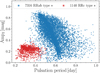 |
Fig. 1 Period-amplitude diagram for RRab and RRc RR Lyrae stars (RRab are shown as blue points, and RRc are shown as red squares) in our final dynamical dataset based on the pulsation properties from the OGLE survey. |
3.1 Interlopers and bulge stars
Interloper stars, which pass through the Galactic bulge, make a substantial contribution to the observed stellar population in this region (25 to 50% Kunder et al. 2020; Lucey et al. 2021, 2022). These stars complicate our understanding of the rotational dynamics of the inner MW. Earlier studies used various methods to reduce the impact of stars from other MW structures, primarily focusing on separation in the apocentric distance and the extent of deviation from the Galactic plane to filter out halo and disk interlopers (see, e.g., Kunder et al. 2020; Lucey et al. 2021, 2022). The distinction between bulge stars and interlopers is typically based on apocentric distance: stars on orbits that are confined within a galactocentric distance of 3.5 kpc are labeled as bulge stars, while those beyond are labeled as interlopers. We note that our definition for bulge and interloper stars connects to their spatial distribution and not to a formation scenario. In our study, we applied the same criteria for apocentric distance to distinguish bulge RR Lyrae stars from other RR Lyrae stars that are not part of the bulge. This decision was partially motivated by Lucey et al. (2023) who found orbits that support the MW’s bar extend vertically up to 3.5 kpc and by the extent of the structure of prograde (in the bar frame) RR Lyrae stars, depicted in Figure 5. We note that some other studies used stars with apocenter distances greater than 3.5 kpc, (e.g., Olivares Carvajal et al. 2024); while here we are interested more in the purity of our bulge sample, and such a cut encompasses the majority of the bulge while limiting contamination from halo and disk stars. Approximately 22% of RR Lyrae in our final kinematical data have rapo > 3.5 kpc, and we refer to these variables as interlopers.
We examine the physical and spatial characteristics of our final dynamical dataset, focusing on how these characteristics correlate with whether a star is more likely part of the bulge or an interloper. Figure 2 illustrates the relationship between the galactocentric spherical radius (rGC) and metallicity with the proportion of interlopers. As expected, the number of interlopers is highest at larger radii compared to the bulge RR Lyrae population. Moreover, the number of RR Lyrae stars not associated with the bulge increases with the distance from the Galactic center, surpassing the number of bulge RR Lyrae stars beyond a radius of 2.5 kpc. A similar conclusion was found in the study of Ardern-Arentsen et al. (2024), where, despite their somewhat different spatial properties (in comparison with our dataset), they noticed a dependence of interloper fraction on the rGC with the number of interloping stars increasing with increasing rGC.
In the metallicity analysis of interloper stars in the Galactic bulge, we observe three key contributors: stars from the Galactic disk, the outer bulge, and the halo. The disk’s RR Lyrae stars are known for their high metallicity (e.g., Layden et al. 1996; Zinn et al. 2020; Prudil et al. 2020; Iorio & Belokurov 2021), whereas the halo’s RR Lyrae stars predominantly occupy the lower metallicity range (Fabrizio et al. 2019, 2021). The variables related to the outer bulge overlap both disk and halo interlopers in metallicity space, which makes distraction and clear separation difficult. This distinction is critical in understanding how each of these MW structures influences the bulge’s interloper population. Based on the metallicity (using photometric metallicities estimated in Prudil et al. 2025) boundaries shown in the right panel of Figure 2 right panel (marked by the shaded gray regions), we find that approximately 25% of the interlopers are likely disk RR Lyrae stars, with the remaining exhibiting halolike (remaining 75% of interlopers) characteristics in their orbits and metallicity. We note that from the identified 25% of the disk interlopers, the majority of stars lie close to the Galactic plane, and only two percent have zmax > 3 kpc. These disk RR Lyrae stars, mostly have rapo between 3.5 kpc and 6 kpc (over 70%) and come from the outer bar region.
In the Appendix, we include Figure D.1, which shows the distribution of orbital frequencies (![Mathematical equation: $\[\Omega_{\phi}^{\text {ine}}\]$](/articles/aa/full_html/2025/07/aa54819-25/aa54819-25-eq8.png) and
and ![Mathematical equation: $\[\Omega_{\phi}^{\text {bar}}\]$](/articles/aa/full_html/2025/07/aa54819-25/aa54819-25-eq9.png) ) in the inertial and bar reference frames for our RR Lyrae dataset. In this figure, we divide the sample into bulge, interlopers, and likely halo RR Lyrae variables (identified by zmax > 5 kpc). In the inertial frame, we do not observe a clear preference for prograde or retrograde rotation among the halo RR Lyrae stars. In the bar frame, however, these pulsators lag behind the rotation of the bar and therefore appear retrograde with respect to the Galactic bar.
) in the inertial and bar reference frames for our RR Lyrae dataset. In this figure, we divide the sample into bulge, interlopers, and likely halo RR Lyrae variables (identified by zmax > 5 kpc). In the inertial frame, we do not observe a clear preference for prograde or retrograde rotation among the halo RR Lyrae stars. In the bar frame, however, these pulsators lag behind the rotation of the bar and therefore appear retrograde with respect to the Galactic bar.
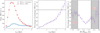 |
Fig. 2 Left: distribution of Galactic bulge (red squares, rapo < 3.5 kpc) and interloping (blue circles, rapo > 3.5 kpc) RR Lyrae as a function of galactocentric radius. Middle: fraction of interloping RR Lyrae as a function of galactocentric radius. Right: fraction of interloping RR Lyrae in bins of photometric metallicity. The highlighted regions mark the boundaries in metallicity for the Galactic halo and disk. |
3.2 Rotation pattern of RR Lyrae variables at different metallicities
Here we explore the dynamical parameter space by looking at the distribution of average vGV and its dispersion across the Galactic longitude bins and for different metallicities. We compare our observational dataset with the bulge model by Shen et al. (2010) which is based on the results from the BRAVA spectroscopic survey (Rich et al. 2007; Howard et al. 2008, 2009). In Figure 3, we display the orbital properties for our entire dataset (blue points) and for bulge RR Lyrae stars with rapo < 3.5 kpc (red squares). The selection based on the apocentric distance to remove interlopers by construction decreases the dispersion in vGV. In the most metal-rich bin of our final dynamical dataset (top left corner of Figure 3), we see clear signs of rotation that follow the bar model of Shen et al. (2010). The dispersion σvGV shows nearly a flat distribution after removing interlopers. This is in agreement with our previous work (Prudil et al. 2025) in which we showed that spatial and transverse properties of metal-rich RR Lyrae ([Fe/H]phot > −1.0 dex) follow the patterns characteristic of the Galactic bar. This is also in agreement with previous studies focused on metal-rich nonvariable giants (e.g., Kunder et al. 2012; Ness et al. 2013b). Here it is important to emphasize that the [Fe/H]phot for the metal-rich bin ([Fe/H]phot > −1.0 dex) is heavely skewed toward [Fe/H]phot ≈ −1.0 dex, with median metallicity (and 15.9 and 84.1 percentiles) of this bin equal to [Fe/H]phot = ![Mathematical equation: $\[-0.75_{-0.18}^{+0.32}\]$](/articles/aa/full_html/2025/07/aa54819-25/aa54819-25-eq10.png) dex. In addition, removing the interlopers (both halo and disk in this case) partially enhances the rotation pattern in the ℓ vs. vGV slightly more pronounced.
dex. In addition, removing the interlopers (both halo and disk in this case) partially enhances the rotation pattern in the ℓ vs. vGV slightly more pronounced.
Considering the metal-poor ([Fe/H]phot = (−1.5; −1.0) dex) population, we find a lag in the average vGV behind the rotation regardless of whether the halo interlopers are removed or not. The dispersion in vGV, as in the metal-rich case, has only a mild difference at ℓ = 0 deg between the full and bulge (no interlopers) RR Lyrae dataset. In this metallicity bin, the halo interlopers do not seem to affect the rotation pattern (their percentage is low, ~14 to 20%). Bins with metallicities below [Fe/H]phot < −1.5 dex start showing a significant contribution from halo interlopers, particularly in the σvGV space where the total sample exhibits higher values for velocity dispersion. We again see a weak rotation that slowly decreases as we move toward lower metallicities. The rotation curve flattens at the metal-poor end of our distribution (RR Lyrae variables with [Fe/H]phot < −2.0 dex).
Here, it is important to stress that the fraction of interlopers differs in each metallicity bin (as seen in Figure 2). We have mostly disk interlopers on the metal-rich side. As we move toward the metal-poor stars, the contribution decreases until we reach [Fe/H]phot = −1.5 dex. Then, the number of stars with apocentric distance above 3.5 kpc (mainly halo RR Lyrae variables) increases again and reaches 40% at the lowest metallicity bin in our sample. Therefore, for RR Lyrae stars, the interlopers affect the rotation pattern only slightly, and their influence is more prominent in the velocity dispersion (particularly the removal of halo interlopers leads to its decrease), especially at the metal-poor end. The presence of interlopers in some cases leads to an increase in the velocity for the rotation curve, which was previously reported by Kunder et al. (2020); Lucey et al. (2021); Ardern-Arentsen et al. (2024). The interlopers are not responsible for the disappearance or lag in rotation. Given that the metal-rich RR Lyrae follow the Galactic bar, both spatially and kinematically (Prudil et al. 2025, and Figure 3 here), other factors must explain the variation in the dynamics of RR Lyrae and other metal-poor populations in the bulge, which we attempt to uncover next.
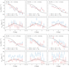 |
Fig. 3 Distribution of the average vGV and its dispersion σvGV in the Galactic longitude bins and for different photometric metallicity cuts. The blue points represent the final dynamical dataset, and the red squares stand for RR Lyrae variables with rapo < 3.5 kpc (labeled BLG in the legend). The dashed lines trace the vGV and σvGV from the bar model of Shen et al. (2010) for b = 4 deg. For this figure, we use equally spaced bins between ℓ = (−8.0; 8.25) deg with a step of 1.25 deg. The asymetric distribution in ℓ was driven by our RR Lyrae dataset. |
4 Orbital properties of the bulge stars
In what follows, we aim to resolve the reason for the differences in the bar-supporting kinematics between the relatively old (≈12 Gyr) RR Lyrae population5 and the relatively young (<10 Gyr) nonvariable giants population. To achieve our goals, we use available kinematical data for nonvariable giants as well as an N-body+SPH simulation together with our RR Lyrae sample.
4.1 Simulation
In this study, we use a high-resolution star-forming N-body+SPH simulation of a galaxy that evolves in isolation. It has been thoroughly described in Cole et al. (2014); Gardner et al. (2014); Debattista et al. (2017); Gough-Kelly et al. (2022); San Martin Fernandez et al. (2025, where it is referred to as HG1) where the simulation was extensively used as a comparison with the MW. The initial setup of this simulation starts with a hot gas corona inside a dark matter halo without any stars. The continued star formation is triggered as the gas corona cools down and settles into a disk, forming a disk galaxy. The model is evolved using the GASOLINE (Wadsley et al. 2004) code for 10 Gyr. At the end of the evolution, it consists of 5 × 10⁶ dark matter particles, and approximately 2.6 × 10⁶ gas and 1.1 × 10⁷ stellar particles. The model forms a bar around 3 Gyr that at 10 Gyr has a length of 3 kpc. In this work, we use snapshots at 1, 2, 4, 5, 6, 7, 8, 9 and 10 Gyr of this simulation.
We explore the orbital parameters and frequencies of the stellar particles located in the central regions. In particular, we adopt the approach of Beraldo e Silva et al. (2023), and use PYNBODY6 (Pontzen et al. 2013) to center and align the simulation snapshots. For each snapshot, we measure the pattern speed, ΩP, using the module7 provided by Dehnen et al. (2023) that estimates pattern speed from individual snapshots. We measure the bar angle (using the inertia tensor approach) in the simulation and align the bar with the x-axis. Using the AGAMA software, we also create a composite potential for each snapshot by describing stellar and gas particles using a triaxial cylspline potential and dark matter halo using an axisymmetric multipole potential. In these potentials, we integrate orbits of randomly selected stellar particles (of all ages) that are located within rGC = 2 kpc. The boundary on spherical radius was motivated by the spatial scaling factor of 1.7 (e.g., Gough-Kelly et al. 2022) often used to match this simulation with the MW’s spatial properties. We emphasize that at this step we did not scale the simulation to match the MW observed properties when computing the orbits (as done in, e.g., Gough-Kelly et al. 2022).
4.2 Data for nonvariable giants
To compare and further explore our results for RR Lyrae stars, we use a dataset with a younger (on average) population provided by the APOGEE DR17 StarHorse value-added catalog (Santiago et al. 2016; Queiroz et al. 2018, 2020). To ensure StarHorse catalog compatibility with our RR Lyrae sample, we mirror their spatial distribution (in Galactic coordinates and distances) with our RR Lyrae dataset and enforce the following set of conditions on the APOGEE DR17 StarHorse catalog:
![Mathematical equation: $\[1.0<\text { Heliocentric distance < } 20 ~\mathrm{kpc}\]$](/articles/aa/full_html/2025/07/aa54819-25/aa54819-25-eq11.png) (6)
(6)
![Mathematical equation: $\[0.0<\log g<3.0 \text { dex. }\]$](/articles/aa/full_html/2025/07/aa54819-25/aa54819-25-eq12.png) (7)
(7)
These conditions ensure that we select preferentially giants (mostly red giants) with distances centered approximately at the Galactic bulge and spatially matching our RR Lyrae dataset. In addition, we remove stars with the following flags in the APOGEE data: PERSIST_HIGH and LOW_SNR. Since we aim to obtain orbital properties for stars in the StarHorse catalog, we selected only objects with Gaia proper motions and APOGEE line-of-sight velocities. Last, similar to our RR Lyrae sample, we applied the criterion from Eq. (1). This yielded a total of 9736 red giants with spatial, kinematic, and chemical information.
As an additional and mostly independent source of nonvariable stars, we used red clump stars identified in the Blanco DECam Bulge Survey (BDBS, Rich et al. 2020; Johnson et al. 2022). This dataset contains photometric metallicities and distances estimated based on the ugrizY passbands. Similar to the pure APOGEE red giant dataset described above, we used the same footprint (in Galactic coordinates and distances) on the red clump. We then crossmatched BDBS red clump stars with the Gaia catalog to obtain proper motions. To derive line-of-sight velocities for BDBS giants, we combined several publicly available surveys, including Gaia (Katz et al. 2023), GALactic Archaeology with HERMES (GALAH, Buder et al. 2021), APOGEE, and GIRAFFE Inner Bulge Survey (Zoccali et al. 2014; Gonzalez et al. 2015). This resulted in 1751 red clump stars with full spatial and kinematic information. Despite our best efforts to identify sources of line-of-sight velocity for the red clump dataset, their spatial distribution does not perfectly match the footprint of RR Lyrae and red giant stars. However, we chose to keep them in our analysis as they represent an additional stellar evolutionary stage.
From here on, we will call the combination of the two samples the nonvariable giant dataset (11 487 objects in total). Its metallicity and spatial distribution in Galactic and Cartesian coordinates are depicted in Figure 4. This Figure shows that our RR Lyrae and nonvariable giants datasets match reasonably well. We note that the nonvariable data do not cover the full extent of our RR Lyrae sample in the region below the Galactic plane, where some of the BRAVA-RR fields reach broader Galactic longitudes.
Similar to our RR Lyrae dataset, we used the analytical model of Portail et al. (2017); Sormani et al. (2022) and Hunter et al. (2024) for the MW implemented in AGAMA (see description in Section 3) to obtain the orbital properties and frequencies (using the naif software of Beraldo e Silva et al. 2023) of our nonvariable giant sample. We used the same integration time of 5 Gyr, as in the case of RR Lyrae stars.
4.3 Bifurcation in orbital parameters, and recovering the rotation pattern for RR Lyrae stars
Here, we combine and examine the data from the simulation (see Section 4.1) with the RR Lyrae and nonvariable giants datasets. In Figure 5 we show the orbital properties for RR Lyrae stars, nonvariable giants, and the simulation. We chose the angular frequency in the bar’s rest frame as an indicator for prograde (positive sign in bar reference frame) and retrograde (negative sign in bar reference frame) stellar motion with respect to the bar. We tested this approach using the parameter, λ, estimated for each time step of the orbit, defined as:
![Mathematical equation: $\[\lambda=L_z-\Omega_{\mathrm{P}} R_{\mathrm{cyl}}^2,\]$](/articles/aa/full_html/2025/07/aa54819-25/aa54819-25-eq13.png) (8)
(8)
where ![Mathematical equation: $\[L_{z}^{\text {ine}}\]$](/articles/aa/full_html/2025/07/aa54819-25/aa54819-25-eq14.png) and Rcyl are the angular momentum and cylindrical radius in the inertial frame. For each star we estimate the median value of λ and compare its sign with the sign of
and Rcyl are the angular momentum and cylindrical radius in the inertial frame. For each star we estimate the median value of λ and compare its sign with the sign of ![Mathematical equation: $\[\Omega_{\varphi}^{\text {rot}}\]$](/articles/aa/full_html/2025/07/aa54819-25/aa54819-25-eq15.png) which we define as:
which we define as:
![Mathematical equation: $\[\Omega_{\varphi}^{\mathrm{rot}}=\Omega_{\varphi}^{\mathrm{ine}}-\Omega_{\mathrm{p}}.\]$](/articles/aa/full_html/2025/07/aa54819-25/aa54819-25-eq16.png) (9)
(9)
We find, in 91% of the cases matching signs, while in the remaining cases, λ oscillates around zero. We note that, by definition, ![Mathematical equation: $\[\Omega_{\varphi}^{\mathrm{rot}}\]$](/articles/aa/full_html/2025/07/aa54819-25/aa54819-25-eq17.png) is the same as
is the same as ![Mathematical equation: $\[\Omega_{\varphi}^{\mathrm{bar}}\]$](/articles/aa/full_html/2025/07/aa54819-25/aa54819-25-eq18.png) . However, in this work, we consider these two quantities to be different. Due to the presence of stars with chaotic orbits (see Section 6 for details), some stars exhibit different signs for
. However, in this work, we consider these two quantities to be different. Due to the presence of stars with chaotic orbits (see Section 6 for details), some stars exhibit different signs for ![Mathematical equation: $\[\Omega_{\varphi}^{\text {rot}}\]$](/articles/aa/full_html/2025/07/aa54819-25/aa54819-25-eq19.png) and
and ![Mathematical equation: $\[\Omega_{\varphi}^{\text {bar}}\]$](/articles/aa/full_html/2025/07/aa54819-25/aa54819-25-eq20.png) . Subsequently, the fraction of stars with matching signs relative to λ (as defined in Eq. (8)) differs for these two quantities, with
. Subsequently, the fraction of stars with matching signs relative to λ (as defined in Eq. (8)) differs for these two quantities, with ![Mathematical equation: $\[\Omega_{\varphi}^{\text {rot}}\]$](/articles/aa/full_html/2025/07/aa54819-25/aa54819-25-eq21.png) showing better agreement with λ than
showing better agreement with λ than ![Mathematical equation: $\[\Omega_{\varphi}^{\mathrm{bar}}\]$](/articles/aa/full_html/2025/07/aa54819-25/aa54819-25-eq22.png) .
.
In Figure 5, we see that stars that fall on the identity line (forming one of the two substructures) between zmax and rapo show almost exclusively negative ![Mathematical equation: $\[\Omega_{\varphi}^{\text {rot}}\]$](/articles/aa/full_html/2025/07/aa54819-25/aa54819-25-eq23.png) and thus retrograde motion with respect to the Galactic bar. These stars, as expected (based on their negative
and thus retrograde motion with respect to the Galactic bar. These stars, as expected (based on their negative ![Mathematical equation: $\[\Omega_{\varphi}^{\text {rot}}\]$](/articles/aa/full_html/2025/07/aa54819-25/aa54819-25-eq24.png) ), to not contribute to the rotation and dispersion trends depicted in the upper panels but rather exhibit counter rotation and a flat dispersion profile. The second substructure, which we will refer to as bulk has positive
), to not contribute to the rotation and dispersion trends depicted in the upper panels but rather exhibit counter rotation and a flat dispersion profile. The second substructure, which we will refer to as bulk has positive ![Mathematical equation: $\[\Omega_{\varphi}^{\text {rot}}\]$](/articles/aa/full_html/2025/07/aa54819-25/aa54819-25-eq25.png) values and clearly follows the rotation and dispersion patterns. From this figure we see that the retrograde orbits are significantly more vertically extended than the prograde orbits. Here and in what follows we use
values and clearly follows the rotation and dispersion patterns. From this figure we see that the retrograde orbits are significantly more vertically extended than the prograde orbits. Here and in what follows we use ![Mathematical equation: $\[\Omega_{\varphi}^{\text {rot}}\]$](/articles/aa/full_html/2025/07/aa54819-25/aa54819-25-eq26.png) as a means to identify and separate prograde and retrograde stars in the Galactic bulge. We opted to use
as a means to identify and separate prograde and retrograde stars in the Galactic bulge. We opted to use ![Mathematical equation: $\[\Omega_{\varphi}^{\text {rot}}\]$](/articles/aa/full_html/2025/07/aa54819-25/aa54819-25-eq27.png) since regular (see Section 6 on regularity) orbits conserve frequencies in barred potentials unlike Lz which is not conserved in nonaxisymmetric potentials.
since regular (see Section 6 on regularity) orbits conserve frequencies in barred potentials unlike Lz which is not conserved in nonaxisymmetric potentials.
The top panels in Figure 5 shows how the positive and negative ![Mathematical equation: $\[\Omega_{\varphi}^{\text {rot}}\]$](/articles/aa/full_html/2025/07/aa54819-25/aa54819-25-eq28.png) manifests in a rotation curve. The nonvariable giants’ sample shows a negligible difference in the rotation pattern between the entire sample (small black dots) and only those with positive
manifests in a rotation curve. The nonvariable giants’ sample shows a negligible difference in the rotation pattern between the entire sample (small black dots) and only those with positive ![Mathematical equation: $\[\Omega_{\varphi}^{\text {rot}}\]$](/articles/aa/full_html/2025/07/aa54819-25/aa54819-25-eq29.png) (pink circles). On the other hand, for RR Lyrae stars, the difference is quite significant. RR Lyrae variables with positive
(pink circles). On the other hand, for RR Lyrae stars, the difference is quite significant. RR Lyrae variables with positive ![Mathematical equation: $\[\Omega_{\varphi}^{\text {rot}}\]$](/articles/aa/full_html/2025/07/aa54819-25/aa54819-25-eq30.png) (yellow squares) expectedly follow a bar rotation pattern while the bulge RR Lyrae dataset is lagging (green points). The reason behind the significant (for RR Lyrae pulsators) and negligible (for nonvariable giants) difference is in the ratio of number of stars with positive versus negative
(yellow squares) expectedly follow a bar rotation pattern while the bulge RR Lyrae dataset is lagging (green points). The reason behind the significant (for RR Lyrae pulsators) and negligible (for nonvariable giants) difference is in the ratio of number of stars with positive versus negative ![Mathematical equation: $\[\Omega_{\varphi}^{\text {rot}}\]$](/articles/aa/full_html/2025/07/aa54819-25/aa54819-25-eq31.png) . Another way of looking at results presented in Figure 5 is that the angular momentum distribution of the RR Lyrae stars is much less tilted towards the prograde Lz.
. Another way of looking at results presented in Figure 5 is that the angular momentum distribution of the RR Lyrae stars is much less tilted towards the prograde Lz.
In the selected bulge fields, for the nonvariable giants populations, we have a fraction of 83% stars with prograde kinematics (see the middle right panel of Figure 5), while for RR Lyrae stars, this probability is ≈72%. If we randomly draw stars from our RR Lyrae dataset with the simple condition that at least 83% of them should have positive ![Mathematical equation: $\[\Omega_{\varphi}^{\text {rot}}\]$](/articles/aa/full_html/2025/07/aa54819-25/aa54819-25-eq32.png) we nearly recover the same rotation pattern as for nonvariable giants. In the bottom panel of Figure 5, we present orbital properties colored by
we nearly recover the same rotation pattern as for nonvariable giants. In the bottom panel of Figure 5, we present orbital properties colored by ![Mathematical equation: $\[\Omega_{\varphi}^{\text {rot}}\]$](/articles/aa/full_html/2025/07/aa54819-25/aa54819-25-eq33.png) for our simulation (snapshot at 10 Gyr). We see that we partially recover the substructures found in the observational data. We notice that the stellar particles with negative
for our simulation (snapshot at 10 Gyr). We see that we partially recover the substructures found in the observational data. We notice that the stellar particles with negative ![Mathematical equation: $\[\Omega_{\varphi}^{\text {rot}}\]$](/articles/aa/full_html/2025/07/aa54819-25/aa54819-25-eq34.png) clump on the identity line, and stellar particles with positive
clump on the identity line, and stellar particles with positive ![Mathematical equation: $\[\Omega_{\varphi}^{\text {rot}}\]$](/articles/aa/full_html/2025/07/aa54819-25/aa54819-25-eq35.png) fall below it. The fraction of particles with negative
fall below it. The fraction of particles with negative ![Mathematical equation: $\[\Omega_{\varphi}^{\text {rot}}\]$](/articles/aa/full_html/2025/07/aa54819-25/aa54819-25-eq36.png) is 14%. We note that in this case, we did not impose any selection criteria on the positions and orbital parameters of the stellar particles.
is 14%. We note that in this case, we did not impose any selection criteria on the positions and orbital parameters of the stellar particles.
Last, in addition to analyzing the stars confined to the Galactic bulge, we also looked at the foreground and background areas of the Galactic bulge. The discussion of objects that fall in these regions is included in Appendix B.
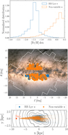 |
Fig. 4 Metallicity (top panel) and spatial distribution in Galactic coordinates (middle panel) and Cartesian coordinates (bottom panel) for datasets of RR Lyrae (blue squares) and nonvariable giants (orange points). The solid white lines in the top panel depict the approximate footprint of the OGLE survey. In the bottom panel, the black lines indicate the surface density contours (of the analytical potential) for a stellar component rotated by the bar angle (25 degrees). The underlying image in the top panel is the Gaiaall-sky star density map. Image credit: ESA/Gaia/DPAC. Images released under CC BY-SA 3.0 IGO. |
5 Implications for the RR Lyrae distribution from orbital frequencies
In this section, we examine in depth the orbital frequencies. We use them to distinguish between different spatial and kinematic populations of RR Lyrae stars within the MW barred potential.
5.1 Metal-poor RR Lyrae stars
Metal-poor giant stars ([Fe/H] < −2.0 dex) are found within the Galactic bulge (e.g., Koch et al. 2016; Arentsen et al. 2020; Rix et al. 2022; Ardern-Arentsen et al. 2024) and a significant fraction (in general over 50%) remains confined to the Galactic bulge. These objects exhibit a slight rotation in vϕ (see Figure 10 in Ardern-Arentsen et al. 2024). However, neither the metal-poor variable nor nonvariable giants seem to follow the Galactic bar spatially and exhibit much slower rotation (if any) compared to the metal-rich population. This can be explained by the high fraction of interlopers (40% of the total sample) and retrograde stars (19% of the total sample) on the metal-poor end of the RR Lyrae metallicity distribution ([Fe/H]phot < −2.0 dex), resulting in only 41% of total metal-poor RR Lyrae stars being associated with the Galactic bar.
We demonstrated previously (see the bottom right panels of Figure 3) that our dataset of RR Lyrae stars shows little to no sign of rotation for metal-poor variables (−2.0 > [Fe/H]phot > −2.6 dex). In Figure 6 we focus on RR Lyrae pulsators with [Fe/H]phot < −2.0 dex that remain on their orbits within the Galactic bulge (defined as rapo < 3.5 kpc). In the metal-poor subset discussed here, retrograde RR Lyrae stars represent approximately 30% of the bulge metal-poor population. The prograde metal-poor RR Lyrae variables in our dataset do not exhibit any preferred location within Galactic coordinates; they are evenly distributed across the analyzed footprint, and presumably well mixed with the dataset presented here.
We note that the observed inconsistency in photometric metallicities for long-period RRab RR Lyrae stars (as described in Hajdu et al. 2018; Jurcsik et al. 2021; Jurcsik & Hajdu 2023) is likely present in our dataset. However, for the following reasons, it does not significantly affect the results outlined above. First, as mentioned in Section 2, the vast majority of our RR Lyrae dataset have distances determined using near-infrared passbands; therefore, the effect on distance is minimal (see Appendix B in Prudil et al. 2025). Second, the ratio of the number of prograde and retrograde RR Lyrae stars remains the same even if we shift our condition on metallicity towards more metal-poor stars8. Thus the rotation and spatial distribution are not affected by the choice of metallicity limit when selecting the two populations.
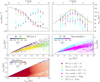 |
Fig. 5 Kinematic and orbital properties for RR Lyrae variables, nonvariable giants, and stellar particles from the simulation. The top panels show the distribution of average vGV and its dispersion σvGV across the Galactic longitude bins. The middle and bottom panels display the distribution of orbital properties zmax vs. rapo for RR Lyrae (middle left panel), nonvariable giants (middle right panel), and model HG1 (bottom left panel, at 10 Gyr). The color-coding in all panels is based on |
![Mathematical equation: $\[\Omega_{\varphi}^{\text {rot}}\]$](/articles/aa/full_html/2025/07/aa54819-25/aa54819-25-eq37.png)
5.2 RR Lyrae stars and B/P bulge
The bimodality in the distance distribution of the bulge red clump stars is well-known (McWilliam & Zoccali 2010; Nataf et al. 2010; Wegg & Gerhard 2013; Lim et al. 2021) and is associated with the X-shape bulge. It is also understood that metal-poor ([Fe/H] < −0.5 dex) red clump stars do not follow a bimodal distance distribution (e.g., Ness et al. 2012; Rojas-Arriagada et al. 2014). In simulations, the presence of a B/P-shaped bulge is often associated with banana-like orbits (Pfenniger & Friedli 1991; Patsis et al. 2002; Martinez-Valpuesta et al. 2006), together with other orbital families (e.g., Portail et al. 2015; Abbott et al. 2017).
In this subsection, we use the calculated orbital and spatial properties to identify RR Lyrae stars that support the B/P-shaped bulge. To identify stars on banana-orbits we used the following condition (similar to the condition in Portail et al. 2015):
![Mathematical equation: $\[1.95<\Omega_{\mathrm{z}}^{\mathrm{bar}} / \Omega_{\mathrm{x}}^{\mathrm{bar}}<2.05\]$](/articles/aa/full_html/2025/07/aa54819-25/aa54819-25-eq38.png) (10)
(10)
where ![Mathematical equation: $\[\Omega_{\mathrm{z}}^{\text {bar}}\]$](/articles/aa/full_html/2025/07/aa54819-25/aa54819-25-eq39.png) and
and ![Mathematical equation: $\[\Omega_{\mathrm{x}}^{\text {bar}}\]$](/articles/aa/full_html/2025/07/aa54819-25/aa54819-25-eq40.png) are orbital frequencies in the bar reference frame. We also follow Portail et al. (2015) in identifying brezel-orbits as
are orbital frequencies in the bar reference frame. We also follow Portail et al. (2015) in identifying brezel-orbits as
![Mathematical equation: $\[1.6<\Omega_{\mathrm{z}}^{\text {bar }} / \Omega_{\mathrm{x}}^{\text {bar }}<1.70.\]$](/articles/aa/full_html/2025/07/aa54819-25/aa54819-25-eq41.png) (11)
(11)
In Figure 7 we show the results of our analysis. The top panel shows how the fraction of stars on banana-orbits changes with metallicity. We see a monotonic increase in the occurrence of banana orbits with metallicity with a plateau at the metal-rich tail. For the metal-rich red clump ([Fe/H] > −0.5 dex) stars in banana orbits represent around 16 to 20% of the total number of orbits, while for metal-poor RR Lyrae stars ([Fe/H]phot < −1.0 dex) they constitute only ≈12% of orbits. A likely explanation of this linear trend is kinematic fractionation (Debattista et al. 2017; Fragkoudi et al. 2018).
The bottom panel of Figure 7 shows the heliocentric distance distribution of our RR Lyrae bulge kinematical dataset. As expected, from previous studies, RR Lyrae stars confined to the Galactic bulge (black histogram) do not exhibit a double-peaked distance distribution. The same can be said when we look at the brezel orbits, which display similar single peak distance distributions. When we consider the RR Lyrae stars on banana orbits however we recover a double-peaked distribution similar to the one seen for metal-rich red clump stars. One of the reasons why we generally do not see a double-peaked RR Lyrae distribution (whole dataset) is the lower fraction of variables on banana orbits compared to the metal-rich nonvariables. As shown in Section 5.3 the number of retrograde orbits increases with decreasing metallicity and such orbits can dilute the potential B/P-shape of the Galactic bulge when traced with RR Lyrae stars.
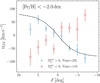 |
Fig. 6 Distribution average vGV across Galactic longitude for metal-poor ([Fe/H] < −2.0 dex) RR Lyrae variables. The blue circles and red squares represent prograde and retrograde RR Lyrae stars, respectively. Here we take bins in Galactic longitude between between −8.0 to 8.0 deg in steps of 2 deg. The dashed line represents the rotation curve for the bar model from Shen et al. (2010) at b = 4 deg. |
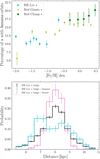 |
Fig. 7 Fraction of banana-orbits on metallicity for the APOGEE red giant (top, yellow circles), BDBS red clump (green pentagons), and RR Lyrae (blue squares) datasets. The bottom panel shows the distance distribution of the RR Lyrae dataset. The black histogram denotes the distances of the bulge RR Lyrae while the blue histogram shows the double-peaked distribution for RR Lyrae stars with banana orbits. The pink histogram shows the RR Lyrae with brezel-orbits which also has a single peak distribution. The uncertainties on individual bins (top panel) were estimated by varying the [Fe/H] by its errors and estimating the fraction of banana orbits in each iteration. For the bottom panel, the uncertainties on each bin represent the Poisson noise. |
5.3 Metallicity, age, and rGC dependence on ![Mathematical equation: $\[\Omega_{\varphi}^{\text {rot}}\]$](/articles/aa/full_html/2025/07/aa54819-25/aa54819-25-eq42.png)
This subsection examines the chemical, age, and spatial properties of the retrograde stars and stellar particles used in this work. As seen in Figure 5, the nonvariable giants and RR Lyrae datasets exhibit different fractions of stars with prograde and retrograde motion with respect to the MW bar. Here, we further explore this difference; in particular, we focus on the difference in ratios of stars with positive and negative ![Mathematical equation: $\[\Omega_{\varphi}^{\text {rot}}\]$](/articles/aa/full_html/2025/07/aa54819-25/aa54819-25-eq43.png) . It is important to emphasize here we use only stars (from the observed data) and stellar particles (rom the simulation) that stay confined within the Galactic bulge, that is, with rapo < 3.5 kpc, as in Sections 3.1 and 4.1. This means that for the simulation we first selected stars within rGC = 2 kpc, then obtained their orbits, and finally applied the condition on apocentric distance. The simulation, after forming the bar (≈3 Gyr), forms an extended nuclear stellar disk that complicates our analysis due to its kinematic properties. Thus, in addition to the criterion on rapo, we decided to also remove stellar particles with zmax < 0.3 kpc to avoid including stellar particles associated with this structure. Likewise, our observational dataset does not cover the MW nuclear stellar disc. The minimum in Galactic latitude for our dataset |b| = 2.0 deg, and the cut for simulation in zmax < 0.3 kpc translates to a similar restriction in Galactic latitude.
. It is important to emphasize here we use only stars (from the observed data) and stellar particles (rom the simulation) that stay confined within the Galactic bulge, that is, with rapo < 3.5 kpc, as in Sections 3.1 and 4.1. This means that for the simulation we first selected stars within rGC = 2 kpc, then obtained their orbits, and finally applied the condition on apocentric distance. The simulation, after forming the bar (≈3 Gyr), forms an extended nuclear stellar disk that complicates our analysis due to its kinematic properties. Thus, in addition to the criterion on rapo, we decided to also remove stellar particles with zmax < 0.3 kpc to avoid including stellar particles associated with this structure. Likewise, our observational dataset does not cover the MW nuclear stellar disc. The minimum in Galactic latitude for our dataset |b| = 2.0 deg, and the cut for simulation in zmax < 0.3 kpc translates to a similar restriction in Galactic latitude.
Figure 8 shows a gradual increase in the number of retrograde stars with respect to the bar as the metallicity of a star decreases. Examining the metal-poor end ([Fe/H] < −1.0 dex) of our observational sample we notice a weak hint of a plateau around [Fe/H] ≈ −1.5 dex. The increase in stars with prograde orbits with metallicity agrees well with previous results on giants toward the Galactic bulge (see, e.g., Arentsen et al. 2020; Lucey et al. 2021) and RR Lyrae stars (Kunder et al. 2020). We recover a similar trend (see the gray line) by performing the binning process for our simulation but in age. There is an increase in bar counter-rotating particles (in the bar’s reference frame) in the older stellar particles as compared to the younger particles (upper axis).
The gradual transition in the fraction of prograde stars with metallicity shown in Figure 8 contrasts with the sharper transition seen in Figure 11 of Marchetti et al. (2024), where a distinct change in kinematic alignment with the bar is observed across metallicity. Their analysis shows a somewhat sharper transition in metallicity space between a clear and diminished dipole pattern, using the correlation between Galactic proper motions as a proxy for rotation. Several factors could explain this discrepancy, including interlopers from other MW substructures, the broad selection function in our sample, or differences in how bar-supporting orbits are defined. Additionally, while the number of red clump stars does decrease significantly below [Fe/H] −0.5 dex, the dominance of metal-rich stars in bar-like orbits, evident in the presence of a double red clump and strong dipole signature, suggests we might expect a sharper kinematic break. The smoother trend in our data could be due to the inclusion of overlapping bulge, bar, and inner disk populations that are not cleanly separated in our orbit-based selection. Notably, in our Figure 8, the most metal-poor bin (≈ −0.35 dex) for red clump stars (that come from BDBS, just like data from Marchetti et al. 2024, study) is significantly higher than the rest of the RR Lyrae and red giant dataset at similar metallicity.
In Figure 9, we show the dependence of ![Mathematical equation: $\[\Omega_{\varphi}^{\text {rot}}\]$](/articles/aa/full_html/2025/07/aa54819-25/aa54819-25-eq46.png) on stellar age and rGC. The stellar ages were taken for our APOGEE Red Giant dataset, from the astroNN value-added catalog (Mackereth et al. 2019). We again consider only stars on orbits that are confined to the Galactic bulge. As expected, based on results depicted in Figure 8, we see an increase of retrograde stars as a function of age (from ages 6 to 10 Gyr). The simulation reproduces the increase as a function of time, but not the fraction of retrograde stars. In the bottom panel of Figure 9 we observe that the fraction of stars on retrograde orbits increases as we move closer to the Galactic center. At radii rGC ≈ 0.5 kpc, the fraction reaches almost 40% for RR Lyrae variables and 35% for APOGEE red giants. The observed increase at smaller rGC likely explains the findings in Kunder et al. (2020) and Olivares Carvajal et al. (2024), where the more centrally concentrated population of RR Lyrae stars does not trace the Galactic bar. Our results indicate that the number of stars with prograde bar-supporting orbits decreases as we move toward the Galactic center. The same trend is also obtained from the simulation, where we observe an increase in retrograde stars for smaller rGC. We note that for our observational dataset, we used a running boxcar with size 100 and step 30 to create Figure 9. In the case of the simulation, we used a box with a size of 1000 and a step equal to 350. We also scaled the spatial coordinates for each stellar particle by a factor of 1.7 (Gough-Kelly et al. 2022) to calculate rGC. This scaling was done to facilitate comparison between the simulation and the observational data since the bar of the model is smaller than that in the MW. The percent of
on stellar age and rGC. The stellar ages were taken for our APOGEE Red Giant dataset, from the astroNN value-added catalog (Mackereth et al. 2019). We again consider only stars on orbits that are confined to the Galactic bulge. As expected, based on results depicted in Figure 8, we see an increase of retrograde stars as a function of age (from ages 6 to 10 Gyr). The simulation reproduces the increase as a function of time, but not the fraction of retrograde stars. In the bottom panel of Figure 9 we observe that the fraction of stars on retrograde orbits increases as we move closer to the Galactic center. At radii rGC ≈ 0.5 kpc, the fraction reaches almost 40% for RR Lyrae variables and 35% for APOGEE red giants. The observed increase at smaller rGC likely explains the findings in Kunder et al. (2020) and Olivares Carvajal et al. (2024), where the more centrally concentrated population of RR Lyrae stars does not trace the Galactic bar. Our results indicate that the number of stars with prograde bar-supporting orbits decreases as we move toward the Galactic center. The same trend is also obtained from the simulation, where we observe an increase in retrograde stars for smaller rGC. We note that for our observational dataset, we used a running boxcar with size 100 and step 30 to create Figure 9. In the case of the simulation, we used a box with a size of 1000 and a step equal to 350. We also scaled the spatial coordinates for each stellar particle by a factor of 1.7 (Gough-Kelly et al. 2022) to calculate rGC. This scaling was done to facilitate comparison between the simulation and the observational data since the bar of the model is smaller than that in the MW. The percent of ![Mathematical equation: $\[\Omega_{\varphi}^{\text {rot}}\]$](/articles/aa/full_html/2025/07/aa54819-25/aa54819-25-eq47.png) is considerably higher at rGC < 0.5 in the observations than in the simulation. This could potentially indicate that the simulation is not exactly the MW (e.g., the difference in age of the bar in the simulation and in the MW) and may also point toward an additional old, spheroidal classical bulge population at small galactocentric radii (as reported in some of the previous studies, see Rix et al. 2022; Belokurov & Kravtsov 2022).
is considerably higher at rGC < 0.5 in the observations than in the simulation. This could potentially indicate that the simulation is not exactly the MW (e.g., the difference in age of the bar in the simulation and in the MW) and may also point toward an additional old, spheroidal classical bulge population at small galactocentric radii (as reported in some of the previous studies, see Rix et al. 2022; Belokurov & Kravtsov 2022).
As shown in Figures 5, 6, 7, and 8 orbital frequencies can separate stars supporting the bar from those that do not support the bar. They can also reveal some previously hidden features in the spatial properties which we explore further in Figure 10 where we depict the spatial distribution in the Cartesian coordinates using kernel density estimates for our RR Lyrae bulge dataset. We split our variable sample into prograde and retrograde based on the sign of the (![Mathematical equation: $\[\Omega_{\varphi}^{\text {rot}}\]$](/articles/aa/full_html/2025/07/aa54819-25/aa54819-25-eq48.png) ). We see that the retrograde RR Lyrae population is more centrally concentrated with a somewhat more circular distribution while prograde RR Lyrae stars have a more elongated shape. To quantify this difference, we measured the bar angle for both the prograde and retrograde RR Lyrae groups. We applied the inertia tensor method, following our previous work (see Section 6 in Prudil et al. 2025), and selected only stars located within 0.2 < |Z| < 0.5 kpc. For the prograde and retrograde populations, we obtained bar angles of ι = 16 ± 3 deg and ι = −5 ± 5 deg, respectively. We note that a smaller value of
). We see that the retrograde RR Lyrae population is more centrally concentrated with a somewhat more circular distribution while prograde RR Lyrae stars have a more elongated shape. To quantify this difference, we measured the bar angle for both the prograde and retrograde RR Lyrae groups. We applied the inertia tensor method, following our previous work (see Section 6 in Prudil et al. 2025), and selected only stars located within 0.2 < |Z| < 0.5 kpc. For the prograde and retrograde populations, we obtained bar angles of ι = 16 ± 3 deg and ι = −5 ± 5 deg, respectively. We note that a smaller value of ![Mathematical equation: $\[R_{\mathrm{cyl}}^{\text {lim }}=1.2\]$](/articles/aa/full_html/2025/07/aa54819-25/aa54819-25-eq49.png) kpc was used to reduce potential selection effects since our kinematic dataset is more spatially constrained and less numerous. As expected, based on orbital frequencies we can detect stars that have bar-supporting orbits, and their selection results in a bar-like feature in their spatial properties.
kpc was used to reduce potential selection effects since our kinematic dataset is more spatially constrained and less numerous. As expected, based on orbital frequencies we can detect stars that have bar-supporting orbits, and their selection results in a bar-like feature in their spatial properties.
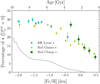 |
Fig. 8 Chemical and orbital properties for the RR Lyrae variable, BDBS red clump star, and APOGEE red giant datasets together with the results from the simulation. The figure shows the dependence of the percentage of retrograde stars as a function of their [Fe/H]. The light blue squares represent metallicity bins for the RR Lyrae sample. The green pentagons and yellow circles represent BDBS stars and APOGEE red giants, respectively. The gray line denotes a fraction of retrograde (negative |
![Mathematical equation: $\[\Omega_{\varphi}^{\text {rot}}\]$](/articles/aa/full_html/2025/07/aa54819-25/aa54819-25-eq44.png)
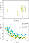 |
Fig. 9 Percentage of stars with negative |
![Mathematical equation: $\[\Omega_{\varphi}^{\text {rot}}\]$](/articles/aa/full_html/2025/07/aa54819-25/aa54819-25-eq45.png)
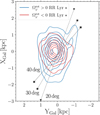 |
Fig. 10 Spatial distribution depicted using the kernel density estimates of the Cartesian coordinates for our RR Lyrae bulge dataset. Blue and red contours show the distributions of prograde and retrograde RR Lyrae stars. The black solid, dashed and dotted lines represent bar angles of 40, 30, and 20 degrees, respectively. The Sun in this perspective would be at YGal = 0 kpc and XGal = −8.2 kpc. |
6 Chaoticity and orbital families of RR Lyrae stars
In this section, we examine the orbital frequencies of our dataset, evaluate their chaoticity (using a parameter describing how much the orbital frequencies are conserved), and identify associated orbital families. Orbital frequencies often serve to identify resonances, distinguish chaotic and regular orbits, and classify orbits into orbital families. We focus only on RR Lyrae variables that satisfy the condition in Eq. (1) and those which stay on their orbit within 3.5 kpc (4877 single-mode RR Lyrae stars). This dataset covers Jacobi integrals, EJ, in the interval EJ = (−2.6, −1.6)/105 [km2 s−2].
To determine whether an orbit is chaotic or regular, we employ two approaches. The first one is based on frequency drift (log10 ΔΩ, also known as frequency diffusion rate, Laskar 1993; Valluri et al. 2010). The frequency drift is defined as the maximum difference in frequencies:
![Mathematical equation: $\[\log _{10} \Delta \Omega=\log _{10}\left(\max \left|\frac{\Omega_i\left(t_2\right)-\Omega_i\left(t_1\right)}{\Omega_i\left(t_1\right)}\right|_{i=1,2,3}\right),\]$](/articles/aa/full_html/2025/07/aa54819-25/aa54819-25-eq50.png) (12)
(12)
where t1 and t2 represent two equal segments of the orbit time interval, and Ωi represents the three frequencies in cylindrical coordinates. For regular orbits, ΔΩ is nearly zero, as regular orbits conserve frequencies, while chaotic orbits exhibit larger ΔΩ values (0.1 and higher). Our second metric of orbit chaoticity is the Lyapunov exponent (Λ, Lyapunov 1992). The Lyapunov exponent measures the sensitivity of orbits to initial conditions by quantifying the rate of exponential separation of initially close trajectories. A higher Lyapunov exponent indicates chaotic behavior of orbits, while lower values suggest more regular behavior. We estimated the Lyapunov exponent using the implementation in AGAMA (Vasiliev 2013).
In Figure 11, we display the estimated chaoticity and regularity properties of the RR Lyrae stars. We particularly investigate the differences in periodicity between prograde and retrograde orbits. Using both metrics—frequency drift and the Lyapunov exponent—we find that the distributions of both orbital groups overlap reasonably well. This indicates that orbits in both groups appear to be similarly chaotic or regular and that retrograde orbits seem to form a somewhat stable structure in the central part of the Galactic bulge.
6.1 Orbital families. The Cartesian coordinate system
Initially, we utilized the combination of fundamental frequencies (time derivatives of the angle variables) in the Cartesian coordinate system (in a bar-rotating frame) to generate frequency maps and automatically identify resonant orbits within our dataset. In frequency maps, resonant orbits are not distributed randomly in the plane, but group together along resonance lines that satisfy the resonant condition k1Ω1 + k2Ω2 + k3Ω3 = 0 (applicable to both Cartesian and cylindrical coordinates), where the vector k = (k1, k2, k3) consists of integers. By examining frequency maps (or frequency ratios), we can discern the majority of orbital families (e.g., Portail et al. 2015; Valluri et al. 2016) associated with various resonances. For simplicity, we classify them into two main groups: tube and box orbits. Tube orbits rotate around the long (x, bar is oriented along the x-axis), intermediate (y)9, or short (z) axes. Conversely, box orbits are mostly nonresonant, and do not have a definite sense of rotation.
In Figure 12, we present a frequency map for our RR Lyrae bulge dataset. A notable observation is the clustering along the short axis z-tubes (diagonal line) and a significant concentration above the z-tube resonance. Furthermore, we observe a high density of stars with negative azimuthal frequency, ![Mathematical equation: $\[\Omega_{\varphi}^{\text {rot}}\]$](/articles/aa/full_html/2025/07/aa54819-25/aa54819-25-eq53.png) , near frequency ratios close to one (
, near frequency ratios close to one (![Mathematical equation: $\[\Omega_{x}^{\text {bar}} / \Omega_{z}^{\text {bar}} \approx 1.0\]$](/articles/aa/full_html/2025/07/aa54819-25/aa54819-25-eq54.png) and
and ![Mathematical equation: $\[\Omega_{y}^{\text {bar}} / \Omega_{z}^{\text {bar}} \approx 1.0\]$](/articles/aa/full_html/2025/07/aa54819-25/aa54819-25-eq55.png) ). The green area marked in Fig. 12 contains orbits exhibiting mainly chaotic behavior.
). The green area marked in Fig. 12 contains orbits exhibiting mainly chaotic behavior.
Among the most populated groups exhibiting prograde motion in the bar frame are the so-called banana orbits, situated at ![Mathematical equation: $\[\Omega_{x}^{\text {bar}} / \Omega_{z}^{\text {bar}}=0.5\]$](/articles/aa/full_html/2025/07/aa54819-25/aa54819-25-eq56.png) . Additionally, the fish-orbits at
. Additionally, the fish-orbits at ![Mathematical equation: $\[\Omega_{x}^{\text {bar}} / \Omega_{z}^{\text {bar}}= 2 / 3\]$](/articles/aa/full_html/2025/07/aa54819-25/aa54819-25-eq57.png) , and the brezel-orbits (
, and the brezel-orbits (![Mathematical equation: $\[\Omega_{x}^{\mathrm{bar}} / \Omega_{z}^{\mathrm{bar}}=3 / 5\]$](/articles/aa/full_html/2025/07/aa54819-25/aa54819-25-eq58.png) , see Portail et al. 2015, and condition in Eq. (11)) are also present (although in low numbers), exhibiting characteristics of both box and tube (z-tube) orbits.
, see Portail et al. 2015, and condition in Eq. (11)) are also present (although in low numbers), exhibiting characteristics of both box and tube (z-tube) orbits.
Conversely, there are few to no orbits at ![Mathematical equation: $\[\Omega_{x}^{\text {bar}} / \Omega_{z}^{\text {bar}}=3 / 4\]$](/articles/aa/full_html/2025/07/aa54819-25/aa54819-25-eq59.png) , as well as other orbits such as
, as well as other orbits such as ![Mathematical equation: $\[\Omega_{x}^{\text {bar}} / \Omega_{z}^{\text {bar}}=4 / 5\]$](/articles/aa/full_html/2025/07/aa54819-25/aa54819-25-eq60.png) and
and ![Mathematical equation: $\[\Omega_{x}^{\text {bar}} / \Omega_{z}^{\text {bar}}= 5 / 6\]$](/articles/aa/full_html/2025/07/aa54819-25/aa54819-25-eq61.png) . A small proportion of the remaining prograde variables fall within the region
. A small proportion of the remaining prograde variables fall within the region ![Mathematical equation: $\[\Omega_{x}^{\mathrm{bar}} / \Omega_{z}^{\mathrm{bar}} \simeq 1.0\]$](/articles/aa/full_html/2025/07/aa54819-25/aa54819-25-eq62.png) and
and ![Mathematical equation: $\[\Omega_{y}^{\mathrm{bar}} / \Omega_{z}^{\mathrm{bar}} \simeq 1.0\]$](/articles/aa/full_html/2025/07/aa54819-25/aa54819-25-eq63.png) , where they can be classified as z-tubes of the x2 orbital family (e.g., Contopoulos & Papayannopoulos 1980). This region also hosts the majority of retrograde RR Lyrae stars, which are centered around
, where they can be classified as z-tubes of the x2 orbital family (e.g., Contopoulos & Papayannopoulos 1980). This region also hosts the majority of retrograde RR Lyrae stars, which are centered around ![Mathematical equation: $\[\Omega_{x}^{\mathrm{bar}} / \Omega_{z}^{\mathrm{bar}}=1.0\]$](/articles/aa/full_html/2025/07/aa54819-25/aa54819-25-eq64.png) and
and ![Mathematical equation: $\[\Omega_{y}^{\mathrm{bar}} / \Omega_{z}^{\mathrm{bar}}=1.0\]$](/articles/aa/full_html/2025/07/aa54819-25/aa54819-25-eq65.png) , at the intersection of z-tube and x-tube resonances.
, at the intersection of z-tube and x-tube resonances.
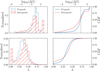 |
Fig. 11 Distribution (left panels) and cumulative distribution functions (right panels) of the frequency drift (top panels) and Lyapunov exponent (bottom panels) for retrograde (red lines) and prograde (blue lines) RR Lyrae stars. The vertical black lines in the upper panels denote our separation between chaotic and regular orbits (see Eq. (13)). |
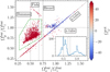 |
Fig. 12 Frequency map illustrating fundamental frequencies in the Cartesian coordinate system and bar-rotating reference frame for our RR Lyrae dataset. The color-coding is used to represent positive and negative values of |
![Mathematical equation: $\[\Omega_{\varphi}^{\text {rot}}\]$](/articles/aa/full_html/2025/07/aa54819-25/aa54819-25-eq51.png)
![Mathematical equation: $\[\Omega_{x}^{\text {bar}}/\Omega_{z}^{\text {bar}}\]$](/articles/aa/full_html/2025/07/aa54819-25/aa54819-25-eq52.png)
6.2 Orbital families. The cylindrical coordinate system
In this subsection, we further explore the association with orbital families based on the frequency maps. We adopt a framework similar to that of Beraldo e Silva et al. (2023) and concentrate on the cylindrical coordinate system in the inertial reference frame. Additionally, we closely examine the orbital shapes associated with various regions of the frequency map, primarily displaying those orbits that exhibit regular behavior (nonchaotic; see the condition in Eq. (13)).
6.2.1 Prograde stars
In Figure 13, we show a frequency map for prograde (in the bar reference frame) RR Lyrae confined to the Galactic bulge in the cylindrical coordinate system and insets depicting orbits, fulfilling the following condition (Valluri et al. 2016):
![Mathematical equation: $\[\log \Delta \Omega<-1.0.\]$](/articles/aa/full_html/2025/07/aa54819-25/aa54819-25-eq66.png) (13)
(13)
Orbits that fulfill this condition are considered regular. For interested readers, we include two additional Figures (Figures D.3 and D.4) with insets depicting different orbital planes in the Appendix D. We divided the frequency map into eight regions and examined the orbits in each selected sector. The level of chaoticity in individual sectors is listed in Table 2. For orbits in each sector, we also estimated the flattening of nonchaotic orbits, which we refer to as circularity in this study. The circularity was estimated as a ratio of the minimum and maximum eigenvalue calculated from each region’s covariance matrix of the ensemble of orbits coordinates (e.g., in Figure 13 for coordinates X and Y). From the circularity we see that orbits in nearly all eight sectors have mostly elongated shapes supporting the bar-like morphology.
In Figure 13, regions 2, 3, and 4 correspond to the inner Lindblad resonance (ILR), the vertical inner Lindblad resonance cloud (vILR cloud, Beraldo e Silva et al. 2023) and the vILR. These regions are densely populated by RR Lyrae variables and overlap with the green area indicated in Figure 12. Sectors 3 and 5, along with regions 2 and 4, have the highest star counts among all regions and contribute to the boxy-peanut shape of the RR Lyrae variables (see Figure D.3). In addition, regions 2 and 3 are occupied by stars with the lowest EJ (confined to the central regions) and Lz among the prograde stars.
From the insets we notice that regions 4, 5, 6, 7, and 8 do not contribute significantly to the Galaxy’s central region, suggesting their association with z-tube orbits, which are located in the x–y plane and revolve around the z-axis. This classification is further confirmed when examining the net angular momentum in the z direction (Lz), which z-tube orbits have (see Figure D.2 in the Appendix). In contrast, variables in regions 1 and 2 display lower chaoticity; interestingly region 2 exhibits a bar-like shape in its face-on projection, while a box-like shape is evident in its side-on projection (see Figure D.3).
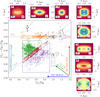 |
Fig. 13 Frequency map showing fundamental frequencies in cylindrical coordinates for prograde RR Lyrae stars in the Galactic bulge dataset. The insets present 2D density maps of the face-on projection (with power-law normalization) of nonchaotic (log ΔΩ < −1.0) orbits in a rotating reference frame for eight selected regions, with high density depicted in blue and low density in red. The insets for each region (marked in the right bottom corner) also contain an estimate of circularity for nonchaotic orbits (bottom left corner) of a given region and the percentage of stars (both with chaotic and periodic orbits) in a given region to the total prograde sample (top left corner). Two significant resonances are identified: the inner Lindblad resonance and the vertical inner Lindblad resonance. |
6.2.2 Retrograde stars
Figure 14 presents the same frequency map as depicted in Figure 13, but for retrograde RR Lyrae stars. We have partitioned the frequency space into six regions and displayed regular orbits (based on condition in Eq. (13)) of each sector in the accompanying insets (in a face-on projection). For side-on and end-on projections of these retrograde RR Lyrae orbits, see Figures D.5 and D.6. In general, stars (both variable and nonvariable) with retrograde orbits have on average lower EJ and |Lz| than their prograde counterparts, meaning that they are more tightly bound to the innermost regions of the Galactic bulge.
A significant difference in the shape of the retrograde orbits compared to the prograde ones is immediately evident. Retrograde RR Lyrae orbits exhibit a rounder shape, whereas their prograde counterparts predominantly display x-axis elongated orbits (looking at the circularity in subplots of Figures 14 and 13). The same applies if we look at the other orbital projections (side-on and end-on) depicted in the Appendix (see Figures D.3, D.4, D.5, and D.6). The spatial distribution of retrograde orbits is more spheroidal while prograde orbits show more ellipsoidal shapes.
We again use the angular momenta (see Figure D.7 in the Appendix) of regular orbits to classify individual sectors into some of the orbital families. Stars in regions 1,5, and 6 exhibit a median nonzero angular momentum in the z direction, indicating that they predominantly follow z-tube orbits. The orbits in the two most numerous and chaotic sectors (3 and 4) are challenging to classify; however, we note that sector 3 shows some net angular momenta in the z direction. Conversely, sectors 1 and 2 display median net angular momenta in the x direction, and coupled with the shape of their orbits, we suggest their classification as x-tube orbits (see insets in Figure D.6).
Expanding on the discussion of chaoticity among retrograde and prograde stars (displayed in Figure 11), the degree of regularity among retrograde RR Lyrae stars appears to be comparable (in median) to that of the prograde moving bulge RR Lyrae variables. For instance, out of the 3429 RR Lyrae stars depicted in the main panel of Figure 13, 52% have log ΔΩ < −1.0. Conversely, in the frequency map of retrograde RR Lyrae variables (Figure 14), we observed 61% of objects fulfilling the aforementioned condition (out of 1374 stars).
As a summary Table 2 lists the median chaoticity values for each region for RR Lyrae and nonvariable datasets. We note the similar frequency of regular orbits for the prograde red giants as for the prograde RR Lyrae variables. The same can also be said about median values of frequency drift and Lyapunov exponent. The only exception seems to be region 8 where RR Lyrae stars appear more chaotic than red giants, but for still the majority of variables in this area show regular orbits.
Figures 13 and 14 show that RR Lyrae stars on retrograde orbits are more abundant in the innermost regions of the Galactic bulge and although metal-poor RR Lyrae stars have a higher tendency to be retrograde, metal-rich stars on retrograde orbits are also present. A population of retrograde stars with high eccentricities can give rise to different features that have been observed previously and attributed to a classical bulge, as discussed more in Section 8.
7 Temporal evolution of the orbits in the simulation
In the previous sections, we confirmed that the older, metal-poor population lags in rotation compared to the younger, metal-rich counterpart (both for variable and nonvariable stars). We also showed that the rotation curve of metal-poor stars can be recovered using orbital frequencies (see Section 5.1). There seems to be a nearly monotonic progression where, as we move from metal-rich to metal-poor stars, the fraction of stars on retrograde orbits (in the bar reference frame) increases. This trend is also recovered when we use stellar ages for our Red Giant dataset. The fraction of retrograde stars increases as we move toward the Galactic center. Similar trends are also observed in the simulation, particularly for the spatial distribution, where we find a good match between RR Lyrae stars and stellar particles of all ages. In the case of RR Lyrae stars, the retrograde orbits seem to be as regular (nonchaotic) as the prograde orbits. Therefore, they can be considered as a spheroidal structure within the Galactic bulge. Since this structure with similar trends in spatial properties and metallicity is also observed in the simulation, we believe it has a secular origin. A secular origin in this context means an internal formation since our simulated galaxy evolved without any accretion event.
The emergence of the retrograde population (in the inertial frame) in this simulation has been previously explored by Fiteni et al. (2021, their model M3_nc_b). They found that approximately 15% of stellar particles within the inner 4 kpc of the simulation have retrograde orbits (based on angular momenta, Lz), and they associate their origin with the bar. All of the retrograde stellar particles in their study for this simulation are found within 4 kpc, and their number increases with time as the bar grows.
In the following, we study the evolution of orbital frequencies as a function of stellar ages (as a proxy for metallicity) by looking at the individual snapshots of the simulation. We use different strategies to analyze the simulation, going beyond that in Sections 4.1 and 5.3. We start by using all stellar particles from a snapshot at 10 Gyr and follow the approach described in Gough-Kelly et al. (2022) to align the simulation with the MW. We adjust its spatial properties by a factor of 1.7 and velocities by a factor of 0.48 to match the bar and bulge characteristics. Additionally, we rotate the stellar particles by 27 degrees around the z-axis to replicate the tilt of the MW bar as estimated by Wegg & Gerhard (2013). Employing coordinate transformation routines implemented in galpy (Bovy 2015), we position the observer at XGC = −8.2 kpc and transform the coordinates and velocities of the stellar particles to Galactic coordinates, distances, and galactocentric velocity vGV. This scaled simulation enables us to select stellar particles with orbital information that approximately matches the footprint of our observational dataset.
We proceed as in Section 4.1 to obtain orbital properties and frequencies of randomly selected stellar particles located within galactocentric radius of 2 kpc. The 2 kpc is the prescaled value equivalent to 3.5 kpc in the MW. The key difference is that now we divide the stellar particles based on their ages into two groups. The first group includes the oldest particles in the simulation born within the first Gyr, while the second group has the younger component born between 4–5 Gyr later. Each group has 100k stellar particles and they map distinct stages in the formation history of the simulated galaxy. The first group forms before the formation of a bar (the bar forms between 2–4 Gyr), and the second group after the bar has formed. For the simulation snapshots at 10, 9, 8, 7, 6, and 5 Gyr we repeated the approach outlined in Section 4.1: we center our simulation using PYNBODY, calculated the pattern speed using the method of Dehnen et al. (2023). We align the bar in our snapshots with the x-axis. We created an analytic potential from each snapshot using AGAMA and integrated orbits for the same stellar particles in each group across snapshots. Here it is important to emphasize that we used the unrescaled model for creating the analytical potential and for the orbit integration. Using this approach, we obtained kinematic properties for the selected stellar particles across multiple snapshots to examine where particles change from prograde to retrograde motion.
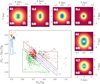 |
Fig. 14 Same as Figure 13, but for retrograde RR Lyrae stars with insets (face-on projection) showing 2D density maps of mostly stable orbits (with log (ΔΩ) < −1). |
7.1 Evolution of bulge stellar particles in frequency maps
To better understand how stellar particles turn from prograde to retrograde motion in the bar reference frame, we must first examine how they evolve in frequency space. In principle stellar particles can turn retrograde, for example, due to a change in pattern speed (as the bar slows down) or due to chaoticity of their orbit. Groundwork on this front has been done by Beraldo e Silva et al. (2023) and is depicted with colored arrows in Figure 13. While Beraldo e Silva et al. (2023) investigated the orbital evolution of particles selected in the shoulder region, that is at the ends of the bar, here we focus on the central parts of the simulation. We use the first group of stellar particles that were born in the first Gyr of the simulation, before the bar’s formation and do not impose any cut or selection on their distribution.
Figure 15 shows the evolution of orbital frequencies for stellar particles from 5 to 10 Gyr, for the prograde stellar particles ((Ωϕ − ΩP)/ΩR > 0). We selected a group of prograde stellar particles around the Ωz/ΩR ≈ 1.0 resonance at 5 Gyr, and traced them throughout the remaining snapshots. This group was selected due to their clear separation from the rest. From this Figure, we see that as the potential evolves, stellar particles move mainly through the vILR to the vILR cloud, and from there, they progress mainly in two directions. A small portion of stellar particles end up in the resonance at Ωz/ΩR = 0.5, while the majority clumps at the ILR. The number of stellar particles at the aforementioned resonances doubles between snapshots at 5 and 10 Gyr, going from 1.5 to 2.9% at Ωz/ΩR = 0.5, and from 19.7 to 43.0% at the ILR (using the same boundaries as in Figure 13). In the last snapshot, the vILR cloud is depopulated and the vast majority of stellar particles are at the ILR or above it. Looking at the evolution for stellar particles that remain prograde throughout the six snapshots the evolution in the frequency map is mainly driven by the decrease of ΩR (preferentially) and Ωϕ although we note that (Ωϕ − ΩP) together with Ωz remain nearly constant.
The frequency map for the retrograde stellar particles can be seen in Figure 16. Looking at the stellar particles that remain retrograde between 5 and 10 Gyr, we see an increase in Ωϕ and Ωz (preferentially). This increase shifts the distribution slightly upwards and toward the right (higher (Ωϕ − ΩP)/ΩR and Ωz/ΩR) as the potential evolves. On the other hand ΩR does not change significantly over the six snapshots. Unlike in the prograde case, (Ωϕ − ΩP) still increases between consecutive snapshots. We note that the particles that remain retrograde throughout the six snapshots are a minority among the total sample (around one percent), and retrograde dataset (seven percent).
To better compare simulation frequency space with our observational dataset we tested how the frequency maps change if we impose the following criteria on orbital properties and Galactic coordinates (to mimic the spatial properties of our observational datasets). We perform the following set of cuts at the 10 Gyr timestep of the simulation:
![Mathematical equation: $\[|\ell|<9^{\circ} ~~\cap~~ r_{\text {apo }}<2 ~\mathrm{kpc} ~~\cap~~ 2^{\circ}<|b|<6^{\circ} ~~\cap~~\left|z_{\max }\right|>0.3 ~\mathrm{kpc}.\]$](/articles/aa/full_html/2025/07/aa54819-25/aa54819-25-eq87.png) (14)
(14)
These cuts reduced our dataset from 100 000 to 34 682 stellar particles. The condition on the maximum value of rapo was used to select only those stars that stay within the bulge (similar to our condition on the observational dataset). In addition, the simulation has a massive nuclear stellar disk, and by applying the cut on zmax we remove all stellar particles associated with this structure. The two remaining criteria on the Galactic coordinates matched stellar particles to our observational footprint. These cuts on the stellar particle distribution do not change our conclusions from the entire dataset.
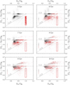 |
Fig. 15 Frequency maps for the same prograde stellar particles in six simulation snapshots. As in Figure 13, we depict two main resonances with dashed lines. The red dots represent stellar particles at resonance around Ωz/ΩR ≈ 1.0 (at 5 Gyr), that we trace to 10 Gyr. |
7.2 Stellar particles before they become retrograde
Using the above-mentioned approach we study the kinematic properties of stellar particles before and after they become retrograde. We focus again on the oldest stellar particles10 in our simulation that were formed before the bar. We look at the percentage of retrograde stellar particles across snapshots from 5 to 10 Gyr, and find a fairly stable value of 20 ± 1% across six snapshots. If we apply the condition in Eq. (14) to this dataset we get 18 ± 1% of particles. Only one percent of the total dataset (seven percent of the retrograde particles) remains retrograde throughout six snapshots, while more than 44 remains prograde. Thus, the remaining 55% of stellar particles during the six snapshots are retrograde at least once. To be specific, in the six analyzed snapshots, 26% of stellar particles turn retrograde once, 13% are retrograde twice, seven percent thrice, six percent four times, and three percent five times. Therefore, we see that the retrograde motion of stellar particles in our six snapshots is mainly temporary, and only a negligible subset remains retrograde long-term. This is expected since Lz is not conserved, resulting in particles (and stars) oscillating between retrograde and prograde motion (in bar reference frame).
We examine the stellar particles in the frequency maps, and by looking at how their angular momentum and Jacobi energy change throughout the analyzed snapshots. We focus on how these two parameters varied during the prograde and retrograde parts of their orbits. To discern between individual stellar particles we decided to group them based on their prograde/retrograde preference. We used the following nomenclature to classify prograde/retrograde changes into sets; if a stellar particle was prograde in three consecutive snapshots we marked it as PPP (three positive ![Mathematical equation: $\[\Omega_{\varphi}^{\text {rot}}\]$](/articles/aa/full_html/2025/07/aa54819-25/aa54819-25-eq88.png) values). If during the second snapshot, stellar particles became retrograde and in the third it became prograde again we denoted them as PRP. Correspondingly stellar particles that were retrograde in three successive snapshots were marked as RRR. To expand on this, if a stellar particle oscillated between being prograde and retrograde we used marks PRPRPR and RPRPRP where the particles in odd and even snapshots switched between prograde and retrograde orbits.
values). If during the second snapshot, stellar particles became retrograde and in the third it became prograde again we denoted them as PRP. Correspondingly stellar particles that were retrograde in three successive snapshots were marked as RRR. To expand on this, if a stellar particle oscillated between being prograde and retrograde we used marks PRPRPR and RPRPRP where the particles in odd and even snapshots switched between prograde and retrograde orbits.
Using the frequency maps and locations of important resonances, particularly the ILR (see Figure 13 for region 2), we looked at the positions of stellar particles right before they became retrograde. These particles, just like the entire population, follow the progression outlined in the previous subsection (see Section 7.1). As the simulation evolves they move from the vILR cloud upward toward the ILR. In Figure 17, we show the evolution in frequency maps for stellar particles that oscillate between prograde and retrograde orbits during six simulation snapshots (marked as PRPRPR). This subgroup represents only a small fraction (below one percent of the total sample) of the total sample but can serve as a good example of the evolution during prograde/retrograde evolution of the same particles. Its evolution in the frequency maps matches well the entire dataset. In Figure 17, we see that the stellar particles do not return to the same frequencies after being prograde/retrograde but they evolve with the rest of the potential toward the ILR.
As the stellar particles oscillate between prograde and retrograde, their Lz and Jacobi energy change. This is depicted in Figure 18 using median values of both quantities for various particle sets (e.g., PPP, PRP, etc.). As the potential evolves the Jacobi energy of stellar particles predictably decreases as particles sink deeper in the potential. This applies across all particle sets, regardless of their prograde/retrograde preference. Regarding the angular momentum, the situation is quite different. In the case of stellar particles that remain prograde in at least three snapshots (PPP), we detect in the first three snapshots a small decrease in angular momentum, that subsequently starts to increase as stellar particles pass through the ILR (their ![Mathematical equation: $\[(\Omega_{\varphi}^{\text {ini}}-\Omega_{\mathrm{P}}) / \Omega_{\mathrm{R}}\]$](/articles/aa/full_html/2025/07/aa54819-25/aa54819-25-eq89.png) increases). Stellar particles that oscillate between prograde and retrograde orbits during three snapshots (PRP) experience first the loss (turning from prograde to retrograde) and then an increase (turning from retrograde to prograde) of angular momentum. The same can be said about stellar particles that during the analyzed snapshots constantly oscillate between prograde and retrograde orbits (PRPRPR) as they repeatedly lose and gain angular momentum. The RRR stellar particles that remain retrograde throughout three consecutive snapshots continue losing angular momentum.
increases). Stellar particles that oscillate between prograde and retrograde orbits during three snapshots (PRP) experience first the loss (turning from prograde to retrograde) and then an increase (turning from retrograde to prograde) of angular momentum. The same can be said about stellar particles that during the analyzed snapshots constantly oscillate between prograde and retrograde orbits (PRPRPR) as they repeatedly lose and gain angular momentum. The RRR stellar particles that remain retrograde throughout three consecutive snapshots continue losing angular momentum.
Furthermore, stellar particles that remained on retrograde orbits (RRRRRR) in all analyzed snapshots are by definition preferentially located at the negative end of the angular momentum distribution and with nearly the lowest Jacobi energies. The same applies also for snapshots before bar formation, where the RRRRRR set had one of the lowest values for angular momentum and Jacobi energy. We note that the RRRRRR set is only a minority (around one percent of the total sample, and seven percent of the retrograde dataset) among the analyzed stellar particles.
Based on Figures 15 and 17 stellar particles evolve toward the ILR. Thus, stellar particles start losing angular momentum (in the z-direction). As the bar loses angular momentum (to the dark matter halo, e.g., Debattista & Sellwood 1998; Athanassoula 2003) it will grow stronger and slow down (its pattern speed will decrease). We see that when a particle turns from prograde to retrograde between two consecutive snapshots, its angular momentum decreases. Inversely, stellar particles that turn from retrograde to prograde orbits gain angular momentum.
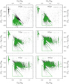 |
Fig. 16 Same as Figure 15, but for retrograde stellar particles (black dots). The green region points to the initial space of the traced particles (green points). |
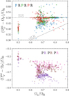 |
Fig. 17 Frequency maps for stellar particles that oscillate between prograde and retrograde orbits with respect to the bar during six analyzed snapshots. In the top panel, we see a frequency map similar to the one in Figure 13 with blue circles (snapshot at 5 Gyr), green squares (snapshot at 7 Gyr) and red triangles (snapshot at 9 Gyr). The bottom panel depicts frequency maps like the one in Figure 14, with purple circles (snapshot at 6 Gyr), brown squares (snapshot at 8 Gyr), and pink triangles (snapshots at 10 Gyr). |
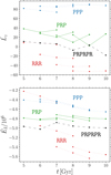 |
Fig. 18 Variation in angular momentum (in the inertial frame, top panel) and Jacobi integral (bottom panel) for various sets of prograde/retrograde stellar particles. The individual lines represent variations of median values of quantities as mentioned across six simulation snapshots. Four different sets of stellar particles are depicted here. Particles that keep their prograde or retrograde orbit (marked as PPP and RRR with dotted lines), and those that oscillate between prograde and retrograde direction (denoted as PRP and PRPRPR with solid and dashed lines). |
7.3 Younger trapped population
Here, we examine the evolution of stellar particles born between 4 and 5 Gyr. These particles were formed after the bar formed in the simulation. To accurately examine this younger dataset, we impose the conditions in Eq. (14) on all the analyses listed in this subsection, to exclude the nuclear stellar disk.
In Section 7.1, we examined how the oldest stellar particles evolved in frequency space. We found that they move mainly through the vILR to the vILR cloud and from there upward to the ILR. Stellar particles born after the formation of the bar move slightly differently. Unlike the oldest stellar particles, the younger objects populate the warm ILR (1.0 < Ωz/ΩR < 1.5, Beraldo e Silva et al. 2023), and from there they move leftward with decreasing Ωz/ΩR (see top panels of Figure 19).
The bottom panels of Figure 19 illustrate the evolution of retrograde stellar particles across six snapshots. In these panels, we present the entire datasets with dotted lines (without applying the condition in Eq. (14)) and a subsample resembling our observational dataset with solid lines (applying the spatial condition in Eq. (14)). Initially, the younger population (green color) exhibits a significant retrograde fraction (![Mathematical equation: $\[\Omega_{\varphi}^{\text {ini}}<\Omega_{\mathrm{P}}\]$](/articles/aa/full_html/2025/07/aa54819-25/aa54819-25-eq90.png) ) and then gets trapped (with
) and then gets trapped (with ![Mathematical equation: $\[\Omega_{\varphi}^{\text {ini}}>\Omega_{\mathrm{P}}\]$](/articles/aa/full_html/2025/07/aa54819-25/aa54819-25-eq91.png) ) and aligns with the bar. Comparing the solid and dotted lines highlights the substantial impact of applying the condition from Eq. (14). Conversely, the overall trend remains consistent: after a few gigayears, the ratio of retrograde younger stellar particles stabilizes with the average percentage of retrograde stellar particles across snapshots from 7 to 10 gigayears equal to 6 ± 1%. We note that this number is related to the sample where the condition of Eq. (14) was applied. The older population (blue color) maintains a relatively constant number of retrograde stars, unaffected by whether conditions replicating our observational footprint are applied or not. Considering both age groups collectively, the ratio of retrograde stars stabilizes around 7 Gyr (approximately 3 Gyr after the bar formed) and remains nearly constant throughout the remainder of the simulation.
) and aligns with the bar. Comparing the solid and dotted lines highlights the substantial impact of applying the condition from Eq. (14). Conversely, the overall trend remains consistent: after a few gigayears, the ratio of retrograde younger stellar particles stabilizes with the average percentage of retrograde stellar particles across snapshots from 7 to 10 gigayears equal to 6 ± 1%. We note that this number is related to the sample where the condition of Eq. (14) was applied. The older population (blue color) maintains a relatively constant number of retrograde stars, unaffected by whether conditions replicating our observational footprint are applied or not. Considering both age groups collectively, the ratio of retrograde stars stabilizes around 7 Gyr (approximately 3 Gyr after the bar formed) and remains nearly constant throughout the remainder of the simulation.
In addition to the previously mentioned two populations we also included stellar particles that formed between 1 and 2 Gyr, that is, before the bar but after the oldest population formed a disk. This intermediate-age population shows a similar trend to the oldest stellar particles with a rather stable retrograde fraction in the bulge. On the other hand, the ratio of retrograde vs. prograde stellar particles is lower than for the oldest population, and percentage-wise, the oldest stellar population still dominates the retrograde distribution.
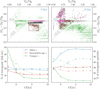 |
Fig. 19 Frequency maps (top panels) and the fraction of retrograde stellar particles (bottom panels) of different ages in several snapshots. The top panels display the distribution of younger stellar particles in frequency maps for two different snapshots. Three groups of stellar particles are selected colored brown, pink and black and brown, in the initial snapshot (left panel, at 5 Gyr) and traced in the following snapshot (right panel at 6 Gyr). Similar to Figure 15, the two main resonances are marked with dashed lines. The bottom panels show the fraction of retrograde stars within the total sample (left bottom panel) and the fraction split by formation age within the retrograde category (for a given snapshot) alone (right bottom panel). The solid lines represent analyses conducted on the dataset where the condition in Eq. (14) was applied, while the dotted lines represent the entire dataset. The blue, red, and green lines represent the oldest (age 9–10 Gyr), intermediate (age 8–9 Gyr), and youngest (age 5–6 Gyr) stellar particles, respectively. |
8 Discussion
The analysis of the N-body+SPH simulation suggests that the origin of retrograde stars in our observational dataset could be a natural progression of the MW bar evolution, particularly the bar’s slow-down and growth. A fraction of retrograde stars in our dataset likely had retrograde orbits (in the inertial frame) even before the bar formed (similar to the finding by Fiteni et al. 2021). Based on their energies and angular momentum, these stars have been part of the central regions (or the bulge) from the very beginning. This may reflect the fact that more centrally concentrated stars, formed from lower angular momentum material, require smaller torques to reverse the direction of their angular momentum vector. After the bar forms, the majority of retrograde stars oscillate between prograde and retrograde orbits.
In the simulation, the percentage of retrograde stars of a given age varies strongly only after the bar forms for the initial 3 Gyr, and then stabilizes. Assuming that the MW bar is at least 6 Gyr old (e.g., Sanders et al. 2024) then Figure 8 reflects a trend over the past few gigayears. The metal-rich RR Lyrae variables ([Fe/H]phot > −1.0 dex) are probably slightly younger (by 1–2 Gyr) and likely initially had more angular momentum compared to the metal-poor RR Lyrae stars (commonly assumed age ≈12 Gyr). This is in contrast with Savino et al. (2020) and highlights the need for a full understanding of the RR Lyrae formation channels. To further strengthen our assumption we need spectroscopically measured [α/Fe] abundances. In the case, where the metal-rich RR Lyrae stars are α-poor, they are likely slightly younger than their metal-poor counterparts. If they turn out to be α-rich, then they would be likely very old (low-mass) RR Lyrae stars.
The results presented here, particularly those in Sections 4, 5, and 6, depend on the selected analytical potential for the MW and its properties. The chosen MW potential affects the number of identified interlopers (e.g., depending on selection criteria and total mass of the potential), but we would not expect this to change our results significantly. However, a significant impact on the results would be selecting an unbarred potential for the MW (e.g., MWPotential2014 or McMillan potentials Bovy 2015; McMillan 2017, as used in some previous studies). By using an axisymmetric analytical potential, we would not observe the bulk structure in zmax vs. rapo plane (see Figure 5). In our case, with a rotating barred potential, the bar properties significantly affect the orbits and estimated frequencies. In Appendix C, we address the dependence of the results presented here on the different values of the bar’s pattern speed.
The effect of uncertainties in the orbital parameters and frequencies examined here has a negligible impact on the presented results. The orbital frequencies are generally significant, and since we focus exclusively on bulge stars, our condition on the apocentric distance (rapo < 3.5 kpc) primarily excludes stars with small ![Mathematical equation: $\[\Omega_{\varphi}^{\text {rot }} \approx 0\]$](/articles/aa/full_html/2025/07/aa54819-25/aa54819-25-eq92.png) . This results in only a minimal chance of misclassifying a star as prograde or retrograde (in the bar reference frame). The bulk structure in the zmax vs. rapo plane remains clearly visible even when we select only stars with high significance in the aforementioned orbital parameters.
. This results in only a minimal chance of misclassifying a star as prograde or retrograde (in the bar reference frame). The bulk structure in the zmax vs. rapo plane remains clearly visible even when we select only stars with high significance in the aforementioned orbital parameters.
We note that, in the following discussion, we do not address recent studies of the central Milky Way and some of its spheroidal features, as discussed in Rix et al. (2022, 2024); Belokurov & Kravtsov (2022). The connection between our dataset and the findings of these studies will be explored in a forthcoming paper.
8.1 Secular spherical bulge
Recent spatial and kinematical studies focusing on the Galactic bulge’s stellar content reveal a prevailing dichotomy between the metal-poor ([Fe/H] ≲ −0.5 dex in metallicity) and metal-rich (approximately > −0.5 dex in metallicity) populations. Metal-poor bulge stars exhibit a more spheroidal spatial distribution with slower rotation, while metal-rich stars predominantly support a barred boxy-peanut bulge spatial distribution and rotation curve (e.g., Zoccali et al. 2017; Rojas-Arriagada et al. 2020; Kunder et al. 2020; Arentsen et al. 2020; Queiroz et al. 2021; Lim et al. 2021; Ardern-Arentsen et al. 2024). The aforementtioned studies sometimes invoked the composite morphology of the MW bulge with both boxy-peanut and classical (product of mergers) components.
Starting from the metal-poor end, Figure 8 shows that the most metal-poor ([Fe/H] < −1.0 dex) stars residing in the Galactic bulge have a high percentage of counter-rotating orbits (≈30%). These objects mostly have boxy orbits (see, e.g., Figure 14) and neither spatially nor kinematically follow the bar as traced from metal-rich red clump stars. The large number of these stars leads to our view of the bulge as more spherical with lagging rotation. If we remove the counter-rotating metal-poor stars, we obtain bulge properties characteristic of their metal-rich counterparts, such as the rotation curve and double-peaked distance distribution (considering only banana-orbits) and a barred spatial distribution (see Figures 6 and 10).
The stars with intermediate metallicities (−1.0 < [Fe/H] < 0.0 dex) have a lower fraction of retrograde stars (between 15 to 25%). Kinematically, they exhibit a rotation curve similar to that of metal-rich stars, and spatially, they show a nearly barred distribution (see, e.g., Lim et al. 2021; Johnson et al. 2022). This intermediate metallicity region is likely sensitive to how close the analyzed dataset is to the Galactic center11, and the metalicity distribution function (MDF) is skewed toward the metal-rich or metal-poor end.
The super metal-rich bulge stars ([Fe/H] > 0.0 dex) are notable for tracing the boxy/peanut shape both spatially and kinematically (e.g., Zoccali et al. 2017). The percentage of counter-rotating stars in this group is low, around 10–15% in our dataset. Despite being the smallest group in terms of percentage, they constitute nearly 40% of retrograde nonvariable giants in absolute numbers for our dataset.
A significant portion of retrograde (in the bar reference frame) stars in the Galactic bulge likely oscillates between prograde and retrograde orbits. According to our simulation analysis, their density compared to generally prograde stars does not change significantly over several gigayears. The orbits of retrograde stars exhibit similar regularity as prograde orbits. Almost all retrograde orbits form a nearly axisymmetric distribution (in the aggregate), contributing to an overall spheroidal distribution in the central parts of the bulge.
There are several reasons why we do not necessarily need to invoke a significant classical bulge in the MW. The currently observed features of the MW bulge can be explained using an N-body+SPH simulation without external influences (e.g., merger events). The difference in the rotation curve between metal-rich and metal-poor stars can be explained, in addition to kinematic fractionation (Debattista et al. 2017; Fragkoudi et al. 2018; Gough-Kelly et al. 2022), by the varying numbers of retrograde stars, which appear to increase linearly with metallicity (see Figure 8). A similar trend can be observed in the increase of retrograde stars towards the central parts of the MW (shown in Figure 9). Last, chemical abundances of bulge nonvariable giants (with metallicities > −1.0 dex), particularly in the [Mg/Mn] vs. [Al/Fe] plane, do not exhibit an over-enhancement of accreted stars (i.e., [Al/Fe]-poor and [Mg/Mn]-rich abundances). Although we note that on the metal-poor side of the metallicity distribution, accreted stars identified using aforementioned abundances could become relevant as discussed in Horta et al. (2021).
Therefore, the observed transition from a metal-rich, barred, cylindrically rotating Galactic bulge to a less barred, slowly rotating bulge can be largely explained by the secular evolution of the MW’s central regions. While we do not completely exclude the contribution of mergers to the Galactic bulge, our analysis points to their potential minimal relevance to the current morphology of the Galactic bulge. Furthermore, the higher fraction of retrograde orbits among metal-poor giants (e.g., RR Lyrae stars) may be a consequence of angular momentum exchange, potentially facilitated by the Galactic bar. Nonetheless, it is also possible that these stars had intrinsically lower angular momentum before the bar was formed.
It is important to emphasize that our results, along with comparisons to N-body+SPH simulations, provide a specific perspective on the formation history of the MW bulge. Further investigation using additional N-body (+SPH) and cosmological simulations would be useful to fully understand the evolution and origin of the retrograde stellar population in the Galactic bulge. On the other hand, we show that a secularly evolved galaxy can form a substructure that, in some of its properties, resembles a classical bulge. The spatial and kinematical characteristics of this substructure can be reasonably well matched with a similar component in the Milky Way bulge.
8.2 Metal-rich RR Lyrae stars
Metal-rich RR Lyrae stars ([Fe/H] > −1.0 dex), as shown in Figures 3, 7, and 8, present a different perspective on the Galactic bulge compared to their metal-poor counterparts. This observation aligns with our previous findings (Prudil et al. 2025) and corroborates the results of other studies (e.g., Kunder et al. 2016; Du et al. 2020). The spatial and kinematic properties of metal-rich RR Lyrae stars closely resemble those of red giants and red clump stars of the same metallicity. Potentially a key to understanding the differences between metal-rich and metal-poor RR Lyrae stars likely lies in their distinct evolutionary pathways, as proposed by Iorio & Belokurov (2021), Bobrick et al. (2024), and Zhang et al. (2025). These studies suggest that metal-rich RR Lyrae stars arise from binary evolution, in contrast to their single-star metal-poor counterparts. Binary interactions may allow these stars to pass through the instability strip at a significantly younger age (compared to single-star evolution), which could explain their bar-like kinematics and spatial distributions.
We examine the red giants in Figure 8 and focus on those corresponding to the most metal-rich bin for RR Lyrae stars. The age distribution of red giants within these metallicity bins, based on the APOGEE value-added catalog (Mackereth et al. 2019), is centered around 8.5 Gyr12, with a significant spread and a non-Gaussian distribution. Notably, approximately 10% of stars in this metallicity bin are younger than 5 Gyr. This finding contrasts with the presumed age distribution of the Galactic bulge, which is predominantly composed of intermediate-age and old stars, with most ages exceeding 5 Gyr (Ortolani et al. 1995; Clarkson et al. 2008; Bensby et al. 2013; Renzini et al. 2018; Joyce et al. 2023). The kinematics of metal-rich RR Lyrae variables suggest they are slightly younger than their metal-poor counterparts, although ages below 8 Gyr appear, in light of our analysis, unlikely.
Last, it is important to note the Galactic bulge does contain old (12–13 Gyr, see Massari et al. 2023), metal-rich RR Lyrae stars within globular clusters NGC 6441 and NGC 6388 (Clementini et al. 2005). These cluster metal-rich RR Lyrae stars have long pulsation periods (≈0.7 day for RRab variables) unlike their thin-disk associated metal-rich counterparts (0.43 day for RRab variables, e.g., Prudil et al. 2020). Then perhaps there must be a formation channel for metal-rich RR Lyrae that does not require binary evolution, for example, helium enrichment as suggested in Savino et al. (2020).
9 Summary
We derived systemic velocities for 8456 RR Lyrae stars. This represents the largest dataset of these variables toward the Galactic bulge assembled to date. We obtained their orbits by integrating their spatial and kinematic properties in an analytical gravitational potential analogous to that of the MW. We separated the RR Lyrae interlopers (22% of our RR Lyrae dataset) that belonged to other MW substructures such as the disk and halo by imposing a condition on the apocentric distance (rapo < 3.5 kpc). We thus removed the variables that are merely passing through the bulge. We note that the population of interlopers within the Galactic bulge significantly depends on the selected analytical potential and their location in the MW. The fraction of interlopers increases steeply with increasing galactocentric radius and Galactic latitude. Approximately 75% of RR Lyrae interlopers can be associated with the Galactic halo, and the remaining 25% spend most of their orbit close to the Galactic plane (zmax < 1 kpc).
The identified interlopers cannot explain the lag that is observed in the bulge rotation curve (as observed in nonvariable giants) in the entire RR Lyrae dataset. A removal of interlopers from our dataset primarily affected the velocity dispersion. A division of our RR Lyrae sample based on their photometric metallicities revealed a variation in the rotation pattern. The rotation patterns of metal-rich RR Lyrae stars ([Fe/H]phot = (0, −1) dex) are those expected from nonvariable giants and confirmed the results from our spatial and transverse velocity analysis (Prudil et al. 2025): This subgroup of RR Lyrae pulsators follows the MW bar. At metal-poor RR Lyrae (−2.0 ≤ [Fe/H]phot ≤ −1.0 dex), the rotation trend slows down and almost entirely disappears for very metal-poor RR Lyrae variables (−2.6 ≤ [Fe/H]phot ≤ −2.0 dex).
Examining the distribution of RR Lyrae pulsators in orbital parameter space (zmax vs. rapo), we observed a bifurcation for variables associated with the Galactic bulge (difference in vertical extent). This bifurcation arises from the inclusion of the Galactic bar in the analytical potential that segregates stars that rotate prograde with the bar (located in the bulk) from those on retrograde orbits (found along the identity line in the zmax vs. rapo plane). A similar structure was also noted for the nonvariable giants. The stars are likely boosted to these orbits when they hit a vertical resonance, probably the vertical inner Lindblad resonance.
To distinguish stars in the two structures, we employed the angular frequency in the bar frame, where negative values align with the identity line, and positive values fall within the observed bulk (see Figure 5). The rotation and dispersion patterns of RR Lyrae stars in orbits that are prograde in the bar frame are clearly consistent with the predictions from simulations and observations of nonvariable giants. Conversely, stars with retrograde orbits in the bar reference frame show counter-rotation and a flat velocity dispersion. Using this criterion on positive and negative ![Mathematical equation: $\[\Omega_{\varphi}^{\text {rot}}\]$](/articles/aa/full_html/2025/07/aa54819-25/aa54819-25-eq93.png) , we also discerned a rotation trend for metal-poor RR Lyrae stars ([Fe/H] < −2.0 dex): 38% are interlopers, 19% exhibit retrograde motion, and only 43% are prograde RR Lyrae stars.
, we also discerned a rotation trend for metal-poor RR Lyrae stars ([Fe/H] < −2.0 dex): 38% are interlopers, 19% exhibit retrograde motion, and only 43% are prograde RR Lyrae stars.
Analyzing the binned metallicity distribution for RR Lyrae and nonvariable giant stars as a function of the percentage of negative ![Mathematical equation: $\[\Omega_{\varphi}^{\text {rot}}\]$](/articles/aa/full_html/2025/07/aa54819-25/aa54819-25-eq94.png) objects, we found a linearly increasing trend in the retrograde fraction from metal-rich to metal-poor stars. This linear increase in the fraction of stars with negative
objects, we found a linearly increasing trend in the retrograde fraction from metal-rich to metal-poor stars. This linear increase in the fraction of stars with negative ![Mathematical equation: $\[\Omega_{\varphi}^{\text {rot}}\]$](/articles/aa/full_html/2025/07/aa54819-25/aa54819-25-eq95.png) is linked to the lag that is observed in the rotation curve for RR Lyrae stars and for metal-poor nonvariable giants. Here, the younger (metal-rich) giant population is less affected by objects on retrograde orbits than the older (metal-poor) population, and it exhibits a clear rotation trend. The analysis of prograde and retrograde orbits showed as expected that stars on prograde orbits have more elongated paths than those on retrograde orbits. In the frequency analysis described in Section 6, we identified several orbital families, and we showed that retrograde stars form a nearly spherical shape in the central parts of the MW (mostly within 2.0 kpc). To further support our conclusions, previous studies using RRab variables demonstrated that the central regions of the Galactic bulge exhibit slower rotation than the outer bulge regions. The latter appears to be more kinematically aligned with the Galactic bar (Kunder et al. 2020; Han et al. 2025). Last, the level of orbit regularity is almost the same for retrograde and prograde orbits. We therefore conclude that the spherical structure supported by the retrograde orbits is a stable substructure within the Galactic bulge.
is linked to the lag that is observed in the rotation curve for RR Lyrae stars and for metal-poor nonvariable giants. Here, the younger (metal-rich) giant population is less affected by objects on retrograde orbits than the older (metal-poor) population, and it exhibits a clear rotation trend. The analysis of prograde and retrograde orbits showed as expected that stars on prograde orbits have more elongated paths than those on retrograde orbits. In the frequency analysis described in Section 6, we identified several orbital families, and we showed that retrograde stars form a nearly spherical shape in the central parts of the MW (mostly within 2.0 kpc). To further support our conclusions, previous studies using RRab variables demonstrated that the central regions of the Galactic bulge exhibit slower rotation than the outer bulge regions. The latter appears to be more kinematically aligned with the Galactic bar (Kunder et al. 2020; Han et al. 2025). Last, the level of orbit regularity is almost the same for retrograde and prograde orbits. We therefore conclude that the spherical structure supported by the retrograde orbits is a stable substructure within the Galactic bulge.
Further analysis using the N-body+SPH simulation showed that the retrograde motion is a long-term motion only for a small subset of stellar particles. The majority of retrograde stellar particles oscillates between prograde and retrograde motion. In the frequency maps, these variations in the orbits occur close to the ILR. Examining stellar particles that were born before or after the formation of the bar, we found that the percentage of retrograde stars does not change significantly for a given age group after the bar forms. This suggests that the trend observed in Figure 8 has likely remained the same for the past few gigayears (assuming the Galactic bar is older than 6 Gyr, Sanders et al. 2024).
We conclude based on our analysis that the previously reported spheroidal feature in the Galactic bulge is a real secondary component. Based on the examined simulation, the spheroidal element can be related to the secular evolution of the Galactic bulge. The evolution is mainly driven by angular momentum exchange and is likely facilitated by the Galactic bar. The flow of angular momentum induces the oscillation between retrograde and prograde orbits. The RR Lyrae stars and some of the nonvariable giants in our study have been part of the inner MW even before the bar was formed. As a result of their low angular momentum, a large fraction of them now oscillate between prograde and retrograde configurations. The stability (i.e., nonchaotic nature) of retrograde orbits, along with their high prevalence, particularly at the metal-poor end of the bulge metallicity distribution function (MDF), can explain certain spatial and kinematic features of the MW bulge that are often attributed to a classical bulge morphology.
We recall that the conclusions we listed above are partially based on secularly evolved simulation; additional investigations with a diverse set of N-body and cosmological simulations would be useful. We showed, however, that a secular evolution can produce a substructure resembling a classical bulge, with spatial and kinematic properties that match those observed in the Milky Way.
Data availability
Full Table 1 is available at the CDS via anonymous ftp to cdsarc.cds.unistra.fr (130.79.128.5) or via https://cdsarc.cds.unistra.fr/viz-bin/cat/J/A+A/699/A349 https://zenodo.org/records/15724090.
Acknowledgements
Z.P. thanks Christian Johnson for providing the BDBS catalog. A.M.K. acknowledges support from grant AST-2009836 from the National Science Foundation. This work has made use of data from the European Space Agency (ESA) mission Gaia (https://www.cosmos.esa.int/gaia), processed by the Gaia Data Processing and Analysis Consortium (DPAC, https://www.cosmos.esa.int/web/gaia/dpac/consortium). Funding for the DPAC has been provided by national institutions, in particular the institutions participating in the Gaia Multilateral Agreement. Funding for the Sloan Digital Sky Survey IV has been provided by the Alfred P. Sloan Foundation, the U.S. Department of Energy Office of Science, and the Participating Institutions. SDSS acknowledges support and resources from the Center for High-Performance Computing at the University of Utah. The SDSS web site is www.sdss4.org. SDSS is managed by the Astrophysical Research Consortium for the Participating Institutions of the SDSS Collaboration including the Brazilian Participation Group, the Carnegie Institution for Science, Carnegie Mellon University, Center for Astrophysics I Harvard & Smithsonian (CfA), the Chilean Participation Group, the French Participation Group, Instituto de Astrofísica de Canarias, The Johns Hopkins University, Kavli Institute for the Physics and Mathematics of the Universe (IPMU)/University of Tokyo, the Korean Participation Group, Lawrence Berkeley National Laboratory, Leibniz Institut für Astrophysik Potsdam (AIP), Max-Planck-Institut für Astronomie (MPIA Heidelberg), Max-Planck-Institut für Astrophysik (MPA Garching), Max-Planck-Institut für Extraterrestrische Physik (MPE), National Astronomical Observatories of China, New Mexico State University, New York University, University of Notre Dame, Observatório Nacional/MCTI, The Ohio State University, Pennsylvania State University, Shanghai Astronomical Observatory, United Kingdom Participation Group, Universidad Nacional Autónoma de México, University of Arizona, University of Colorado Boulder, University of Oxford, University of Portsmouth, University of Utah, University of Virginia, University of Washington, University of Wisconsin, Vanderbilt University, and Yale University. This research made use of the following Python packages: Astropy (Astropy Collaboration 2013, 2018), PYNBODY (Pontzen et al. 2013), emcee (Foreman-Mackey et al. 2013), AGAMA (Vasiliev 2019), IPython (Pérez & Granger 2007), Matplotlib (Hunter 2007), NumPy (Harris et al. 2020), and SciPy (Virtanen et al. 2020).
Appendix A Estimation of line-of-sight and systemic velocities from available spectra
To estimate systemic velocities, vsys, from available spectra, we proceeded in the same way for all three spectral sources (BRAVA-RR, APOGEE, and program ID 093.B-0473) with only minor adjustments due to different spectral ranges. We used photometric information in the OGLE and Gaia survey for all targeted RR Lyrae stars (pulsation periods, time of brightness maxima, and peak-to-peak amplitudes in I and G-band).
To derive vsys we first measure the line-of-sight velocities, vlos, for available spectra. We use the iSpec package Blanco-Cuaresma et al. (2014); Blanco-Cuaresma (2019) for this procedure (spectral synthesis and line-of-sight velocity determination). We proceed in a similar way as in Prudil et al. (2024b); we first synthesize a grid of spectra with physical parameters covering the typical ranges for RR Lyrae stars (based on stellar parameters found in the literature; e.g., Sneden et al. 2017; Crestani et al. 2021a,b), with the following stellar parameters:
Teff = (6000, 6500, 7000, 7500) K
log g = (2.0, 2.5, 3.0) dex
[Fe/H] = (−2.5, −2.0, −1.5, −1.0, −0.5, 0.0) dex
Microturbulence velocity ξturb = 3.5 km s−1
We also needed to synthesize different spectral ranges based on three spectral sources used in our study. We used 8450–8720 Å for BRAVA-RR to mimic spectral ranges from Gaia (Katz et al. 2023) that were used for creating line-of-sight velocity templates and scaling relations. For the APOGEE survey, we used the 15 000–17 000 Å range, and for data from the FLAMES GIRAFFE spectrograph, we used the 5200–5700 Å range. All of the aforementioned synthetic spectra were created using iSpec, and its wrapper for radiative transfer code, MOOG (February 2017 version, Sneden 1973), in combination with the ATLAS9 model atmosphere (Castelli & Kurucz 2003), lines from the VALD database13, and solar scale (Asplund et al. 2009).
In estimating vlos, we proceeded in the following way. In the first step, we estimated vlos using all synthesized spectra for a given observed spectrum. The synthesized spectrum that resulted in the lowest scatter in the vlos was selected for the final vlos calculation, where we varied the fluxes of observed spectra within their uncertainties (assuming they follow a Gaussian distribution) and in each iteration recorded the vlos (200 interactions in total). Similar to Prudil et al. (2024b), we used the bootstrap method to estimate the average and standard deviation of vlos and its variation, σvlos. In Figure A.1, we show the distribution of uncertainties on estimated line-of-sight velocities for fundamental and first overtone RR Lyrae stars. Using the observation time and coordinates on the sky, we performed Heliocentric correction for each measured vlos and estimated the Heliocentric Julian date of the observation, THJD.
A.1 Systemic velocities
We divided our procedure based on the spectra source to determine vsys of individual stars. In the case of BRAVA-RR and APOGEE data, we used our newly derived line-of-sight velocity templates and scaling relations for RRab and RRc variables (Prudil et al. 2024b). For spectra from the VLT/FLAMES program 093.B-0473 we used templates and scaling relations from Braga et al. (2021). Their templates for Fe lines include the majority of features present in these spectra. We note that there is a partial overlap in RR Lyrae variables between the three spectral sources (four objects in common). We did not combine vlos to estimate vsys since our dataset covers different spectral ranges that require different treatments to estimate vsys. Variables that have data from more than one source were used to verify derived systemic velocities and their uncertainties. The estimated line-of-sight velocities for some of the analyzed spectra exhibited unreliable measurements. Thus, we decided to employ the following conditions on the significance of vlos:
![Mathematical equation: $\[\left|v_{\text {los }} / \sigma_{v_{\text {los }}}\right|>10 \qquad \text { OR } \qquad \sigma_{v_{\text {los }}}<20 \mathrm{~km} \mathrm{~s}^{-1}\]$](/articles/aa/full_html/2025/07/aa54819-25/aa54819-25-eq96.png) (A.1)
(A.1)
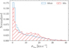 |
Fig. A.1 The distribution of σvlos for our sample of RR Lyrae stars, the blue and red histograms represent uncertainties for RRab and RRc variables. |
These two conditions preserved stars with vlos around zero that still have low σvlos. If a given vlos and σvlos did not fulfill one of the conditions above, it was not used in subsequent systemic velocity determination.
For the determination of vsys of individual RR Lyrae stars, we draw inspiration from our previous work (Prudil et al. 2024b). The calculation of vsys is an optimization problem with a set of data and model parameters. Therefore, we used the Bayesian approach (Bayes & Price 1763) that the following equation can summarize:
![Mathematical equation: $\[p(\boldsymbol{\theta} \mid \mathbf{D}) \propto p(\mathbf{D} \mid \boldsymbol{\theta}) p(\boldsymbol{\theta})\qquad,\]$](/articles/aa/full_html/2025/07/aa54819-25/aa54819-25-eq97.png) (A.2)
(A.2)
where p(θ|D) represents a posterior probability for a model θ given data D, variable p(D|θ) is the likelihood function and p(θ) is the prior on model parameters. Data for a given star in our spectroscopic sample can be described as:
![Mathematical equation: $\[\mathbf{D}=\left\{P, M_0, \mathrm{Amp}_{\text {los }}, \sigma_{\mathrm{Amp}_{\text {los }}}, v_{\text {los }}, \sigma_{v_{\text {los }}}, T_{\mathrm{HJD}}\right\}\qquad.\]$](/articles/aa/full_html/2025/07/aa54819-25/aa54819-25-eq98.png) (A.3)
(A.3)
The amplitudes for line-of-sight velocity curves and their associated errors (Amplos and σAmplos) were determined in the following way. For stars in the Gaia RR Lyrae catalogue (Clementini et al. 2023) we used their AmpG, while for variables that did not have AmpG, we used OGLE peak-to-peak amplitudes (AmpI), and converted to AmpG using relations from Prudil et al. (2024b, see Eqs. 10 and 12).
To convert the amplitudes from G-passband to Amplos for BRAVA-RR and APOGEE spectra, we also used equations from Prudil et al. (2024b). In the case of spectra from the 093.B-0473 program, we used relations from Prudil et al. (2024b, see Eqs. 11 and 13) to convert our G-band magnitudes to AmpV and subsequently to Amplos through relations from Braga et al. (2021) for Fe lines. We propagated uncertainties, using covariance matrices from Prudil et al. (2024b), in case of relations from Braga et al. (2021), we refitted the relations to estimate the correlation (ρRRab = 0.99 and ρRRc = 0.97) between parameters to construct the covariance matrix. Here, it is important to emphasize that Braga et al. (2021) uses as a time reference, M0, the time of the mean magnitude along the rising branch for 093.B-0473 spectra. We used the same reference point instead of the M0 determined by the OGLE team.
θ for a given pulsator is represented by the vsys and a phase shift Δphase. The phase shift parameter was implemented to mitigate the possible effects of imprecision in M0. These can be caused by the data analysis (in case of a low number of observations) or related to a given RR Lyrae star, for instance, modulations of light curves (Netzel et al. 2018; Prudil et al. 2017; Prudil & Skarka 2017; Skarka et al. 2020) or binarity (Hajdu et al. 2015; Prudil et al. 2019b; Hajdu et al. 2021). For the phase shift, we selected the following prior:
![Mathematical equation: $\[p(\boldsymbol{\theta})=n\left(\Delta_{\text {phase}} \mid 0.0,0.1\right) ~\cap~\left|\Delta_{\text {phase}}\right|<0.3\qquad.\]$](/articles/aa/full_html/2025/07/aa54819-25/aa54819-25-eq99.png) (A.4)
(A.4)
Here 𝑛 represents the normal distribution. The central value at 0.0 and a small spread equal to 0.1 were motivated by our initial expectation that our calculated phases would not shift significantly due to the above-mentioned effects. Last, the likelihood p(Dk | θk) for given k-star we defined as:
![Mathematical equation: $\[p\left(\mathbf{D} \mid v_{\mathrm{sys}}\right)=n\left(v_{\mathrm{los}}^{\mathrm{model}} \mid v_{\mathrm{los}}, \sigma_{\mathrm{data}}^{\mathrm{model}}\right)\qquad,\]$](/articles/aa/full_html/2025/07/aa54819-25/aa54819-25-eq100.png) (A.5)
(A.5)
where ![Mathematical equation: $\[v_{\text {los}}^{\text {model}}\]$](/articles/aa/full_html/2025/07/aa54819-25/aa54819-25-eq101.png) represents predicted line-of-sight velocities estimated based on the line-of-sight velocity templates and spectrophotometric data. We defined the
represents predicted line-of-sight velocities estimated based on the line-of-sight velocity templates and spectrophotometric data. We defined the ![Mathematical equation: $\[v_{\text {los}}^{\text {model}}\]$](/articles/aa/full_html/2025/07/aa54819-25/aa54819-25-eq102.png) in the same way as in Prudil et al. (2024b) for BRAVA-RR and APOGEE data, therefore using both the template TempRR and the scatter along the template Temp
in the same way as in Prudil et al. (2024b) for BRAVA-RR and APOGEE data, therefore using both the template TempRR and the scatter along the template Temp![Mathematical equation: $\[_{\text {err}}^{\mathrm{RR}}\]$](/articles/aa/full_html/2025/07/aa54819-25/aa54819-25-eq103.png) . For the 093.B-0473 program spectra, we used only the template from Braga et al. (2021).
. For the 093.B-0473 program spectra, we used only the template from Braga et al. (2021).
For each star, we maximalized the posterior log-probability defined in the Eq. A.2 with priors and likelihood described in Equations A.4 and A.5 using the EMCEE package (Foreman-Mackey et al. 2013). For each star, we used 50 walkers for 4000 steps. Subsequently, we thinned the samples by τ = 10 and discarded the initial 3900 samples. The resulting posterior distribution of parameters θk was then used to estimate the vsys its uncertainty, σvsys, and shift in phase, Δphase.
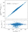 |
Fig. A.2 The comparison of determined systemic velocities with literature values (BRAVA-RR systemic velocities, Kunder et al. 2020) and using our approach for BRAVA-RR spectra. |
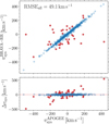 |
Fig. A.3 The same as Figure A.2 but comparing with APOGEE spectra and values determined by BRAVA-RR (Kunder et al. 2020). The red points mark stars with extremely different systemic velocities estimated based on APOGEE and BRAVA-RR spectra and do not pass the condition in Equation 1. |
A.2 Comparison of systemic velocities
Here, we compare our determine systemic velocities for BRAVA-RR and APOGEE spectra with the systemic velocities estimated by Kunder et al. (2020) in the original BRAVA-RR Data Release 2. We note that Butler et al. (2024) conducted a similar comparison between BRAVA-RR and APOGEE velocities, finding good agreement between APOGEE line-of-sight velocities and individual line-of-sight measurements from the Ca Triplet.
In Figure A.2, we measured our determined systemic velocities and the systemic velocities estimated by BRAVA-RR (![Mathematical equation: $\[v_{\text {sys}}^{\text {BRAVA}-\text {RR}}\]$](/articles/aa/full_html/2025/07/aa54819-25/aa54819-25-eq104.png) ). For the comparison, we used only variables marked with Flag = 0 from Kunder et al. (2020). In total, 2213 systemic velocities for single-mode RR Lyrae stars were compared. We found a mild scatter (assessed based on the root-mean-square error, RMSE) between our values and values determined in Kunder et al. (2020) that was most likely a result of an updated approach in the vsys determination.
). For the comparison, we used only variables marked with Flag = 0 from Kunder et al. (2020). In total, 2213 systemic velocities for single-mode RR Lyrae stars were compared. We found a mild scatter (assessed based on the root-mean-square error, RMSE) between our values and values determined in Kunder et al. (2020) that was most likely a result of an updated approach in the vsys determination.
Figure A.3 shows a comparison of systemic velocities determined here based on BRAVA-RR data Kunder et al. (2020, again, using only those with Flag = 0) and vsys estimated from the APOGEE spectra. We see a larger scatter than in the previous comparison (BRAVA-RR velocities only), most likely caused by several different sources. First, APOGEE spectra have, in general, lower S/Ns than BRAVA-RR spectra, resulting in increased uncertainties of individual vlos. Second, APOGEE in most cases provides only a single epoch measurement, which in the case of low-S/N spectra can lead to inaccurate vsys determination. Third, the line-of-sight velocity templates and amplitude scaling relations for estimating vsys from APOGEE spectra are based only on a few RR Lyrae variables, thus contributing to the large scatter in the comparison.
In this Figure, we also see that some of the analyzed RR Lyrae stars have extremely different estimated systemic velocities between APOGEE and BRAVA-RR datasets (marked with red points). Particularly, we noticed that 34 RR Lyrae stars in the comparison (seven percent of the dataset for comparison) exhibit more than 50 km s−1 difference in the determined systemic velocities. From these 34 RR Lyrae stars, nine do not pass the criteria in Eq. 1 and their discrepant systemic velocity can be explained by a blended signal with a nearby star. Two stars from the remaining 25 objects have different Gaia source_id’s in our dataset and the APOGEE catalog. We note that the detected outliers do not show significantly lower S/N than other APOGEE RR Lyrae stars and the APOGEE flags also do not provide additional information that would shed light on the clear reason behind their discrepacy. We note that we prioritized BRAVA-RR RR Lyrae systemic velocities over those derived based on APOGEE data. Last, the average difference between both estimated systemic velocity datasets equals 0.8 km s−1. Thus, we do not detect any significant offset between both surveys.
In conclusion, our derived systemic velocities match reasonably well with the literature values. The discrepancies in the individual vsys are partially covered by the uncertainties that are on average 4 km s−1 and 8 km s−1 for BRAVA-RR and APOGEE vsys, respectively.
Appendix B Foreground and background of the Galactic bulge
Here, we focus on the population in the foreground and background (based on their orbital properties) of the Galactic bulge. The orbital properties of nonvariable giants are compared with our RR Lyrae kinematical dataset in Figure B.1. This image focuses on the orbital properties in zmax and rapo space for both datasets. In particular, we explore their approximate orbital association with the MW’s substructures, disk, and halo (roughly separated by a boundary using zmax values). We noticed that most bulge RR Lyrae interlopers come from the Galactic halo, while for nonvariable giants, most of the interlopers come from the Galactic disk or the outer bulge. We see that many interloper stars still have mostly positive ![Mathematical equation: $\[\Omega_{\varphi}^{\text {rot}}\]$](/articles/aa/full_html/2025/07/aa54819-25/aa54819-25-eq105.png) , for example prograde motion with respect to the Galactic bar, for 83% of RR Lyrae stars and 96% of nonvariable giants (with the apocentric distances between 3.5 kpc and 7.0 kpc).
, for example prograde motion with respect to the Galactic bar, for 83% of RR Lyrae stars and 96% of nonvariable giants (with the apocentric distances between 3.5 kpc and 7.0 kpc).
This suggests that when examining the distribution of line-of-sight velocities for stars toward the Galactic bulge, we will see more younger stars on prograde orbits (disk and outer bulge origin) with respect to the bar than older ones. Thus, this will affect spectroscopic surveys and studies predominantly targeting younger/metal-rich populations toward the Galactic bulge. Without taking into account whether these objects are actually located in the Galactic bulge, they will find a preferential rotation trend with the Galactic bar. This is different for the metal-poor population, which is mostly associated with the Galactic halo and contributes less to the rotation pattern of stars located toward the Galactic bulge. We note that this effect contributes only marginally and cannot explain the lag in the rotation for the older metal-poor population.
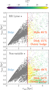 |
Fig. B.1 The distribution of orbital properties zmax vs. rapo for RR Lyrae (top panel) and nonvariable giants stars (bottom panel). The color-coding is based on values of |
![Mathematical equation: $\[\Omega_{\varphi}^{\text {ine}}-\Omega_{\mathrm{P}}\]$](/articles/aa/full_html/2025/07/aa54819-25/aa54819-25-eq106.png)
Appendix C Dependence of orbital properties on pattern speed
Here we explore if and how our results change if we apply a different value for the ΩP. We focus on the change in the pattern speed since we expect it to correlate with the bar length. The value for the pattern speed used in this study and for the applied model in AGAMA was ΩP = 37.5 km s−1 kpc−1. We note that other values for the ΩP appear in the literature, ranging between 30–60 km s−1 kpc−1, meaning that the MW either has a long-slow or a fast-short bar (see, e.g., Debattista et al. 2002; Antoja et al. 2014; Sormani et al. 2015; Portail et al. 2017; Clarke & Gerhard 2022). In addition, an even smaller estimate for the bar pattern speed was recently presented by Horta et al. (2025, ΩP = 24 km s−1 kpc−1) using the APOGEE survey data.
We explore the effect of different pattern speeds on the results presented here by recalculating the orbital properties and frequencies using a set of values for ΩP = 24, 30, 37.5, 40, 50 km s−1 kpc−1. We only tested these values for our RR Lyrae kinematical dataset, but we do not expect any significant differences for red giants and red clump stars analyzed here. For all five values of ΩP we looked at zmax vs. rapo space and found a similar bulk structure (similar to the one found in the middle panels of Figure 5) and nearly the same rotation pattern (using angular frequency in the bar frame, top panels of Figure 5). The percentage of halo and disk interlopers remains the same (within one to two percent) across all values of ΩP as for our fiducial value. The same can be said about the fraction of retrograde and prograde RR Lyrae stars, which does not change, more than one to two percent, from values reported in Section 4. The trend in circularity for nonchaotic orbits also matches our results in Section 6, the prograde moving RR Lyrae stars exhibit a more bar-like shape while retrograde variables show more circular orbits.
In Figure C.1 we observe differences in the overall distribution of stars in the frequency maps (both for prograde and retrograde). The prograde frequency maps constructed using lower values for ΩP appear more evolved, in the sense that regions 5, 7, and 8 are more depopulated, and significantly more stars are located in regions 2 and 3 (ILR and vILR cloud). This results in a higher number of prograde stars with chaotic orbits (log ΔΩ < −1.0) for lower values of ΩP. The retrograde side of the frequency map also shows differences between lower and higher values of ΩP. Regions 2 and 6 (depicted, e.g., in Figure 14) are more populated for lower ΩP than for higher values of the pattern speed, while other regions exhibit the opposite trend. The exception here is region 4 which shows a similar fraction or number of stars throughout the various values for pattern speed.
Since for lower ΩP we see an increased number of stars in the regions of the ILR and the vILR cloud and for regions 2 and 6 on the retrograde side, this results in a larger difference in overall regularity of orbits between the prograde and retrograde part of our dataset. For lower values of the pattern speed, the retrograde stars have on average more regular orbits (in both frequency drift and the Lyapunov coefficient), while for larger values of ΩP the difference in chaoticity between prograde and retrograde orbits decreases. Our test showed that values in Table 2 strongly depend on the selected pattern speed, particularly the number of stars in each region. The overall trend however remains the same, orbits of prograde moving RR Lyrae stars exhibit ellipsoidal distribution while retrograde orbits have spherical shapes.
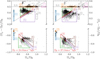 |
Fig. C.1 Two frequency maps showing fundamental frequencies in cylindrical coordinates for two pattern speeds, ΩP = 24 km s−1 kpc−1 (left panels) and ΩP = 37.5 km s−1 kpc−1 (right panels). Only bulge RR Lyrae variables fulfilling conditions in Eq. 1 are depicted. Similar to Figures 13 and 14 we depict analyzed regions. |
Appendix D Additional images
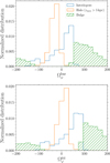 |
Fig. D.1 The distribution of interloping (blue histogram) and bulge (green histogram) RR Lyrae stars. In addition, we include likely halo RR Lyrae stars selected based on their zmax. |
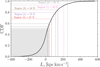 |
Fig. D.2 Cumulative distribution of Lz for bulge RR Lyrae stars (black solid line). The dotted color lines (same as depicted in Figure 13) represent median angular momentum values for the regular orbits in five regions (4, 5, 6, 7, and 8). The dashed lines and gray lines depict median Lz for regions 1, 2, and 3. The filled gray rectangle outlines percentile 50 and lower for Lz. |
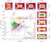 |
Fig. D.3 Same as Figure 13 for prograde RR Lyrae stars but in the insets we display orbits in the x vs. z plane (side on projection). |
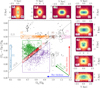 |
Fig. D.4 Same as Figure 13 for prograde RR Lyrae stars but in the insets we display orbits in the y vs. z plane (end on projection). |
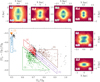 |
Fig. D.5 Same as Figure 14 for retrograde RR Lyrae stars but in the insets we display orbits in the x vs. z plane (side on projection). |
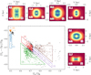 |
Fig. D.6 Same as Figure 14 for retrograde RR Lyrae stars but in the insets we display orbits in the y vs. z plane (end on projection). |
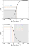 |
Fig. D.7 Similar to Figure D.2 we display cumulative distribution for Lx (top panel) and Lz (bottom panel) of our retrograde RR Lyrae dataset. With color-coded dotted lines, we highlighted the median angular momenta values for selected regions from the retrograde frequency map (Figure 14). The filled gray rectangles outline percentile 50 and lower for Lx and 50 and higher for Lz. |
References
- Abbott, C. G., Valluri, M., Shen, J., & Debattista, V. P. 2017, MNRAS, 470, 1526 [NASA ADS] [CrossRef] [Google Scholar]
- Adams, F. C., Bloch, A. M., Butler, S. C., Druce, J. M., & Ketchum, J. A. 2007, ApJ, 670, 1027 [Google Scholar]
- Alcock, C., Allsman, R. A., Alves, D. R., et al. 1998, ApJ, 492, 190 [NASA ADS] [CrossRef] [Google Scholar]
- Anderson, S. R., Gough-Kelly, S., Debattista, V. P., et al. 2024, MNRAS, 527, 2919 [Google Scholar]
- Antoja, T., Helmi, A., Dehnen, W., et al. 2014, A&A, 563, A60 [NASA ADS] [CrossRef] [EDP Sciences] [Google Scholar]
- Ardern-Arentsen, A., Monari, G., Queiroz, A. B. A., et al. 2024, MNRAS, 530, 3391 [NASA ADS] [CrossRef] [Google Scholar]
- Arentsen, A., Starkenburg, E., Martin, N. F., et al. 2020, MNRAS, 491, L11 [Google Scholar]
- Asplund, M., Grevesse, N., Sauval, A. J., & Scott, P. 2009, ARA&A, 47, 481 [NASA ADS] [CrossRef] [Google Scholar]
- Astropy Collaboration (Robitaille, T. P., et al.) 2013, A&A, 558, A33 [NASA ADS] [CrossRef] [EDP Sciences] [Google Scholar]
- Astropy Collaboration (Price-Whelan, A. M., et al.) 2018, AJ, 156, 123 [Google Scholar]
- Athanassoula, E. 2003, MNRAS, 341, 1179 [Google Scholar]
- Athanassoula, E. 2005, MNRAS, 358, 1477 [NASA ADS] [CrossRef] [Google Scholar]
- Baade, W. 1946, PASP, 58, 249 [NASA ADS] [CrossRef] [Google Scholar]
- Babusiaux, C., & Gilmore, G. 2005, MNRAS, 358, 1309 [NASA ADS] [CrossRef] [Google Scholar]
- Bayes, M., & Price, M. 1763, Philos. Trans. Roy. Soc. Lond. Ser. I, 53, 370 [Google Scholar]
- Beaulieu, S. F., Freeman, K. C., Kalnajs, A. J., Saha, P., & Zhao, H. 2000, AJ, 120, 855 [Google Scholar]
- Belokurov, V., & Kravtsov, A. 2022, MNRAS, 514, 689 [NASA ADS] [CrossRef] [Google Scholar]
- Bensby, T., Yee, J. C., Feltzing, S., et al. 2013, A&A, 549, A147 [NASA ADS] [CrossRef] [EDP Sciences] [Google Scholar]
- Beraldo e Silva, L., Debattista, V. P., Anderson, S. R., et al. 2023, ApJ, 955, 38 [NASA ADS] [CrossRef] [Google Scholar]
- Blanco-Cuaresma, S. 2019, MNRAS, 486, 2075 [Google Scholar]
- Blanco-Cuaresma, S., Soubiran, C., Heiter, U., & Jofré, P. 2014, A&A, 569, A111 [CrossRef] [EDP Sciences] [Google Scholar]
- Blanton, M. R., Bershady, M. A., Abolfathi, B., et al. 2017, AJ, 154, 28 [Google Scholar]
- Bobrick, A., Iorio, G., Belokurov, V., et al. 2024, MNRAS, 527, 12196 [Google Scholar]
- Bovy, J. 2015, ApJS, 216, 29 [NASA ADS] [CrossRef] [Google Scholar]
- Braga, V. F., Crestani, J., Fabrizio, M., et al. 2021, ApJ, 919, 85 [NASA ADS] [CrossRef] [Google Scholar]
- Buder, S., Sharma, S., Kos, J., et al. 2021, MNRAS, 506, 150 [NASA ADS] [CrossRef] [Google Scholar]
- Butler, D., Carbon, D., & Kraft, R. P. 1976, ApJ, 210, 120 [Google Scholar]
- Butler, E., Kunder, A., Prudil, Z., et al. 2024, ApJ, 963, L33 [NASA ADS] [CrossRef] [Google Scholar]
- Castelli, F., & Kurucz, R. L. 2003, in Modelling of Stellar Atmospheres, 210, eds. N. Piskunov, W. W. Weiss, & D. F. Gray, A20 [Google Scholar]
- Catelan, M. 2009, Ap&SS, 320, 261 [Google Scholar]
- Chatzopoulos, S., Fritz, T. K., Gerhard, O., et al. 2015, MNRAS, 447, 948 [Google Scholar]
- Chiba, R., & Schönrich, R. 2022, MNRAS, 513, 768 [NASA ADS] [CrossRef] [Google Scholar]
- Chiba, R., Friske, J. K. S., & Schönrich, R. 2021, MNRAS, 500, 4710 [Google Scholar]
- Clarke, J. P., & Gerhard, O. 2022, MNRAS, 512, 2171 [NASA ADS] [CrossRef] [Google Scholar]
- Clarkson, W., Sahu, K., Anderson, J., et al. 2008, ApJ, 684, 1110 [NASA ADS] [CrossRef] [Google Scholar]
- Clementini, G., Gratton, R. G., Bragaglia, A., et al. 2005, ApJ, 630, L145 [Google Scholar]
- Clementini, G., Ripepi, V., Garofalo, A., et al. 2023, A&A, 674, A18 [NASA ADS] [CrossRef] [EDP Sciences] [Google Scholar]
- Cole, D. R., Debattista, V. P., Erwin, P., Earp, S. W. F., & Roškar, R. 2014, MNRAS, 445, 3352 [NASA ADS] [CrossRef] [Google Scholar]
- Combes, F., & Sanders, R. H. 1981, A&A, 96, 164 [NASA ADS] [Google Scholar]
- Combes, F., Debbasch, F., Friedli, D., & Pfenniger, D. 1990, A&A, 233, 82 [NASA ADS] [Google Scholar]
- Contopoulos, G., & Papayannopoulos, T. 1980, A&A, 92, 33 [NASA ADS] [Google Scholar]
- Crestani, J., Braga, V. F., Fabrizio, M., et al. 2021a, ApJ, 914, 10 [Google Scholar]
- Crestani, J., Fabrizio, M., Braga, V. F., et al. 2021b, ApJ, 908, 20 [Google Scholar]
- Debattista, V. P., & Sellwood, J. A. 1998, ApJ, 493, L5 [Google Scholar]
- Debattista, V. P., Gerhard, O., & Sevenster, M. N. 2002, MNRAS, 334, 355 [Google Scholar]
- Debattista, V. P., Carollo, C. M., Mayer, L., & Moore, B. 2004, ApJ, 604, L93 [NASA ADS] [CrossRef] [Google Scholar]
- Debattista, V. P., Mayer, L., Carollo, C. M., et al. 2006, ApJ, 645, 209 [Google Scholar]
- Debattista, V. P., Ness, M., Gonzalez, O. A., et al. 2017, MNRAS, 469, 1587 [Google Scholar]
- Dehnen, W., Semczuk, M., & Schönrich, R. 2023, MNRAS, 518, 2712 [Google Scholar]
- Dékány, I., Minniti, D., Catelan, M., et al. 2013, ApJ, 776, L19 [Google Scholar]
- D’Orazi, V., Storm, N., Casey, A. R., et al. 2024, MNRAS, 531, 137 [CrossRef] [Google Scholar]
- Du, H., Mao, S., Athanassoula, E., Shen, J., & Pietrukowicz, P. 2020, MNRAS, 498, 5629 [CrossRef] [Google Scholar]
- Dwek, E., Arendt, R. G., Hauser, M. G., et al. 1995, ApJ, 445, 716 [CrossRef] [Google Scholar]
- Einasto, J. 1965, Trudy Astrofiz. Inst. Alma-Ata, 5, 87 [NASA ADS] [Google Scholar]
- Erkal, D., Belokurov, V., Laporte, C. F. P., et al. 2019, MNRAS, 487, 2685 [Google Scholar]
- Fabrizio, M., Bono, G., Braga, V. F., et al. 2019, ApJ, 882, 169 [Google Scholar]
- Fabrizio, M., Braga, V. F., Crestani, J., et al. 2021, ApJ, 919, 118 [NASA ADS] [CrossRef] [Google Scholar]
- Fiteni, K., Caruana, J., Amarante, J. A. S., Debattista, V. P., & Beraldo e Silva, L. 2021, MNRAS, 503, 1418 [NASA ADS] [CrossRef] [Google Scholar]
- Foreman-Mackey, D., Hogg, D. W., Lang, D., & Goodman, J. 2013, PASP, 125, 306 [Google Scholar]
- Fragkoudi, F., Di Matteo, P., Haywood, M., et al. 2018, A&A, 616, A180 [NASA ADS] [CrossRef] [EDP Sciences] [Google Scholar]
- Fragkoudi, F., Grand, R. J. J., Pakmor, R., et al. 2020, MNRAS, 494, 5936 [Google Scholar]
- Gaia Collaboration (Prusti, T., et al.) 2016, A&A, 595, A1 [NASA ADS] [CrossRef] [EDP Sciences] [Google Scholar]
- Gaia Collaboration (Vallenari, A., et al.) 2023, A&A, 674, A1 [NASA ADS] [CrossRef] [EDP Sciences] [Google Scholar]
- Gardner, E., Debattista, V. P., Robin, A. C., Vásquez, S., & Zoccali, M. 2014, MNRAS, 438, 3275 [Google Scholar]
- Gonzalez, O. A., Rejkuba, M., Zoccali, M., et al. 2011, A&A, 530, A54 [NASA ADS] [CrossRef] [EDP Sciences] [Google Scholar]
- Gonzalez, O. A., Zoccali, M., Vasquez, S., et al. 2015, A&A, 584, A46 [NASA ADS] [CrossRef] [EDP Sciences] [Google Scholar]
- Gough-Kelly, S., Debattista, V. P., Clarkson, W. I., et al. 2022, MNRAS, 509, 4829 [Google Scholar]
- Gratton, R. G., Tornambe, A., & Ortolani, S. 1986, A&A, 169, 111 [Google Scholar]
- Hajdu, G., Catelan, M., Jurcsik, J., et al. 2015, MNRAS, 449, L113 [NASA ADS] [CrossRef] [Google Scholar]
- Hajdu, G., Dékány, I., Catelan, M., Grebel, E. K., & Jurcsik, J. 2018, ApJ, 857, 55 [Google Scholar]
- Hajdu, G., Pietrzyński, G., Jurcsik, J., et al. 2021, ApJ, 915, 50 [NASA ADS] [CrossRef] [Google Scholar]
- Han, X., Wang, H.-F., Carraro, G., et al. 2025, ApJ, 985, 32 [Google Scholar]
- Harris, C. R., Millman, K. J., van der Walt, S. J., et al. 2020, Nature, 585, 357 [NASA ADS] [CrossRef] [Google Scholar]
- Horta, D., Schiavon, R. P., Mackereth, J. T., et al. 2021, MNRAS, 500, 1385 [Google Scholar]
- Horta, D., Petersen, M. S., & Peñarrubia, J. 2025, MNRAS, 538, 998 [Google Scholar]
- Howard, C. D., Rich, R. M., Reitzel, D. B., et al. 2008, ApJ, 688, 1060 [NASA ADS] [CrossRef] [Google Scholar]
- Howard, C. D., Rich, R. M., Clarkson, W., et al. 2009, ApJ, 702, L153 [NASA ADS] [CrossRef] [Google Scholar]
- Hunter, J. D. 2007, Comput. Sci. Eng., 9, 90 [NASA ADS] [CrossRef] [Google Scholar]
- Hunter, G. H., Sormani, M. C., Beckmann, J. P., et al. 2024, A&A, 692, A216 [NASA ADS] [CrossRef] [EDP Sciences] [Google Scholar]
- Iorio, G., & Belokurov, V. 2021, MNRAS, 502, 5686 [Google Scholar]
- Johnson, C. I., Rich, R. M., Simion, I. T., et al. 2022, MNRAS, 515, 1469 [NASA ADS] [CrossRef] [Google Scholar]
- Joyce, M., Johnson, C. I., Marchetti, T., et al. 2023, ApJ, 946, 28 [NASA ADS] [CrossRef] [Google Scholar]
- Jurcsik, J., & Hajdu, G. 2023, MNRAS, 525, 3486 [NASA ADS] [CrossRef] [Google Scholar]
- Jurcsik, J., Hajdu, G., & Juhász, Á. 2021, MNRAS, 505, 2468 [NASA ADS] [CrossRef] [Google Scholar]
- Katz, D., Sartoretti, P., Guerrier, A., et al. 2023, A&A, 674, A5 [NASA ADS] [CrossRef] [EDP Sciences] [Google Scholar]
- Koch, A., McWilliam, A., Preston, G. W., & Thompson, I. B. 2016, A&A, 587, A124 [NASA ADS] [CrossRef] [EDP Sciences] [Google Scholar]
- Kormendy, J., & Kennicutt, Robert C., J. 2004, ARA&A, 42, 603 [NASA ADS] [CrossRef] [Google Scholar]
- Kunder, A., Koch, A., Rich, R. M., et al. 2012, AJ, 143, 57 [NASA ADS] [CrossRef] [Google Scholar]
- Kunder, A., Rich, R. M., Koch, A., et al. 2016, ApJ, 821, L25 [CrossRef] [Google Scholar]
- Kunder, A., Pérez-Villegas, A., Rich, R. M., et al. 2020, AJ, 159, 270 [NASA ADS] [CrossRef] [Google Scholar]
- Kunder, A., Prudil, Z., Skaggs, C., et al. 2024, AJ, 168, 139 [NASA ADS] [Google Scholar]
- Laskar, J. 1993, Physica D: Nonlinear Phenomena, 67, 257 [NASA ADS] [CrossRef] [Google Scholar]
- Layden, A. C., Hanson, R. B., Hawley, S. L., Klemola, A. R., & Hanley, C. J. 1996, AJ, 112, 2110 [NASA ADS] [CrossRef] [Google Scholar]
- Leung, H. W., Bovy, J., Mackereth, J. T., et al. 2023, MNRAS, 519, 948 [Google Scholar]
- Lim, D., Lee, Y.-W., Koch, A., et al. 2021, ApJ, 907, 47 [NASA ADS] [CrossRef] [Google Scholar]
- Lucey, M., Hawkins, K., Ness, M., et al. 2021, MNRAS, 501, 5981 [NASA ADS] [CrossRef] [Google Scholar]
- Lucey, M., Hawkins, K., Ness, M., et al. 2022, MNRAS, 509, 122 [Google Scholar]
- Lucey, M., Pearson, S., Hunt, J. A. S., et al. 2023, MNRAS, 520, 4779 [NASA ADS] [CrossRef] [Google Scholar]
- Lyapunov, A. M. 1992, Int. J. Control, 55, 531 [CrossRef] [Google Scholar]
- Lynden-Bell, D., & Kalnajs, A. J. 1972, MNRAS, 157, 1 [Google Scholar]
- Mackereth, J. T., Bovy, J., Leung, H. W., et al. 2019, MNRAS, 489, 176 [Google Scholar]
- Majewski, S. R., Schiavon, R. P., Frinchaboy, P. M., et al. 2017, AJ, 154, 94 [NASA ADS] [CrossRef] [Google Scholar]
- Marchetti, T., Joyce, M., Johnson, C. I., et al. 2024, A&A, 682, A96 [NASA ADS] [CrossRef] [EDP Sciences] [Google Scholar]
- Martinez-Valpuesta, I., Shlosman, I., & Heller, C. 2006, ApJ, 637, 214 [NASA ADS] [CrossRef] [Google Scholar]
- Massari, D., Aguado-Agelet, F., Monelli, M., et al. 2023, A&A, 680, A20 [NASA ADS] [CrossRef] [EDP Sciences] [Google Scholar]
- McMillan, P. J. 2017, MNRAS, 465, 76 [NASA ADS] [CrossRef] [Google Scholar]
- McWilliam, A., & Rich, R. M. 1994, ApJS, 91, 749 [NASA ADS] [CrossRef] [Google Scholar]
- McWilliam, A., & Zoccali, M. 2010, ApJ, 724, 1491 [NASA ADS] [CrossRef] [Google Scholar]
- Merritt, D., & Sellwood, J. A. 1994, ApJ, 425, 551 [NASA ADS] [CrossRef] [Google Scholar]
- Minniti, D., White, S. D. M., Olszewski, E. W., & Hill, J. M. 1992, ApJ, 393, L47 [NASA ADS] [CrossRef] [Google Scholar]
- Minniti, D., Alcock, C., Alves, D., et al. 1998, in The Central Regions of the Galaxy and Galaxies, 184, ed. Y. Sofue, 123 [Google Scholar]
- Minniti, D., Lucas, P. W., Emerson, J. P., et al. 2010, New A, 15, 433 [Google Scholar]
- Nataf, D. M., Udalski, A., Gould, A., Fouqué, P., & Stanek, K. Z. 2010, ApJ, 721, L28 [NASA ADS] [CrossRef] [Google Scholar]
- Ness, M., Freeman, K., Athanassoula, E., et al. 2012, ApJ, 756, 22 [NASA ADS] [CrossRef] [Google Scholar]
- Ness, M., Freeman, K., Athanassoula, E., et al. 2013a, MNRAS, 430, 836 [CrossRef] [Google Scholar]
- Ness, M., Freeman, K., Athanassoula, E., et al. 2013b, MNRAS, 432, 2092 [CrossRef] [Google Scholar]
- Ness, M., Zasowski, G., Johnson, J. A., et al. 2016, ApJ, 819, 2 [NASA ADS] [CrossRef] [Google Scholar]
- Netzel, H., Smolec, R., Soszyński, I., & Udalski, A. 2018, MNRAS, 480, 1229 [NASA ADS] [Google Scholar]
- Olivares Carvajal, J., Zoccali, M., De Leo, M., et al. 2024, A&A, 687, A312 [NASA ADS] [CrossRef] [EDP Sciences] [Google Scholar]
- Ortolani, S., Renzini, A., Gilmozzi, R., et al. 1995, Nature, 377, 701 [CrossRef] [Google Scholar]
- Papaphilippou, Y., & Laskar, J. 1996, A&A, 307, 427 [NASA ADS] [Google Scholar]
- Papaphilippou, Y., & Laskar, J. 1998, A&A, 329, 451 [NASA ADS] [Google Scholar]
- Patsis, P. A., Skokos, C., & Athanassoula, E. 2002, MNRAS, 337, 578 [NASA ADS] [CrossRef] [Google Scholar]
- Pérez, F., & Granger, B. E. 2007, Comput. Sci. Eng., 9, 21 [Google Scholar]
- Pfenniger, D., & Friedli, D. 1991, A&A, 252, 75 [NASA ADS] [Google Scholar]
- Pietrukowicz, P., Udalski, A., Soszyński, I., et al. 2012, ApJ, 750, 169 [NASA ADS] [CrossRef] [Google Scholar]
- Pietrukowicz, P., Kozłowski, S., Skowron, J., et al. 2015, ApJ, 811, 113 [Google Scholar]
- Pontzen, A., Roškar, R., Stinson, G. S., et al. 2013, Astrophysics Source Code Library [record ascl:1305.002] [Google Scholar]
- Portail, M., Wegg, C., & Gerhard, O. 2015, MNRAS, 450, L66 [NASA ADS] [CrossRef] [Google Scholar]
- Portail, M., Gerhard, O., Wegg, C., & Ness, M. 2017, MNRAS, 465, 1621 [NASA ADS] [CrossRef] [Google Scholar]
- Prudil, Z., & Skarka, M. 2017, MNRAS, 466, 2602 [NASA ADS] [CrossRef] [Google Scholar]
- Prudil, Z., Smolec, R., Skarka, M., & Netzel, H. 2017, MNRAS, 465, 4074 [Google Scholar]
- Prudil, Z., Dékány, I., Grebel, E. K., et al. 2019a, MNRAS, 487, 3270 [Google Scholar]
- Prudil, Z., Skarka, M., Liška, J., Grebel, E. K., & Lee, C. U. 2019b, MNRAS, 487, L1 [Google Scholar]
- Prudil, Z., Dékány, I., Grebel, E. K., & Kunder, A. 2020, MNRAS, 492, 3408 [Google Scholar]
- Prudil, Z., Hanke, M., Lemasle, B., et al. 2021, A&A, 648, A78 [NASA ADS] [CrossRef] [EDP Sciences] [Google Scholar]
- Prudil, Z., Koch-Hansen, A. J., Lemasle, B., et al. 2022, A&A, 664, A148 [NASA ADS] [CrossRef] [EDP Sciences] [Google Scholar]
- Prudil, Z., Kunder, A., Dékány, I., & Koch-Hansen, A. J. 2024a, A&A, 684, A176 [NASA ADS] [CrossRef] [EDP Sciences] [Google Scholar]
- Prudil, Z., Smolec, R., Kunder, A., Koch-Hansen, A. J., & Dékány, I. 2024b, A&A, 685, A153 [NASA ADS] [CrossRef] [EDP Sciences] [Google Scholar]
- Prudil, Z., Kunder, A., Beraldo e Silva, L., et al. 2025, A&A, 695, A211 [NASA ADS] [CrossRef] [EDP Sciences] [Google Scholar]
- Queiroz, A. B. A., Anders, F., Santiago, B. X., et al. 2018, MNRAS, 476, 2556 [Google Scholar]
- Queiroz, A. B. A., Anders, F., Chiappini, C., et al. 2020, A&A, 638, A76 [NASA ADS] [CrossRef] [EDP Sciences] [Google Scholar]
- Queiroz, A. B. A., Chiappini, C., Perez-Villegas, A., et al. 2021, A&A, 656, A156 [NASA ADS] [CrossRef] [EDP Sciences] [Google Scholar]
- Quillen, A. C. 2002, AJ, 124, 722 [NASA ADS] [CrossRef] [Google Scholar]
- Quillen, A. C., Minchev, I., Sharma, S., Qin, Y.-J., & Di Matteo, P. 2014, MNRAS, 437, 1284 [Google Scholar]
- Raha, N., Sellwood, J. A., James, R. A., & Kahn, F. D. 1991, Nature, 352, 411 [Google Scholar]
- Renzini, A., Gennaro, M., Zoccali, M., et al. 2018, ApJ, 863, 16 [NASA ADS] [CrossRef] [Google Scholar]
- Rich, R. M. 1988, AJ, 95, 828 [NASA ADS] [CrossRef] [Google Scholar]
- Rich, R. M., Reitzel, D. B., Howard, C. D., & Zhao, H. 2007, ApJ, 658, L29 [NASA ADS] [CrossRef] [Google Scholar]
- Rich, R. M., Johnson, C. I., Young, M., et al. 2020, MNRAS, 499, 2340 [NASA ADS] [CrossRef] [Google Scholar]
- Rix, H.-W., Chandra, V., Andrae, R., et al. 2022, ApJ, 941, 45 [NASA ADS] [CrossRef] [Google Scholar]
- Rix, H.-W., Chandra, V., Zasowski, G., et al. 2024, ApJ, 975, 293 [NASA ADS] [CrossRef] [Google Scholar]
- Rojas-Arriagada, A., Recio-Blanco, A., Hill, V., et al. 2014, A&A, 569, A103 [NASA ADS] [CrossRef] [EDP Sciences] [Google Scholar]
- Rojas-Arriagada, A., Zasowski, G., Schultheis, M., et al. 2020, MNRAS, 499, 1037 [Google Scholar]
- Salaris, M., & Girardi, L. 2002, MNRAS, 337, 332 [NASA ADS] [CrossRef] [Google Scholar]
- San Martin Fernandez, L. M., Gough-Kelly, S., Debattista, V. P., et al. 2025, MNRAS, 540, 2506 [Google Scholar]
- Sanders, J. L., Smith, L., & Evans, N. W. 2019, MNRAS, 488, 4552 [NASA ADS] [CrossRef] [Google Scholar]
- Sanders, J. L., Kawata, D., Matsunaga, N., et al. 2024, MNRAS, 530, 2972 [NASA ADS] [CrossRef] [Google Scholar]
- Santiago, B. X., Brauer, D. E., Anders, F., et al. 2016, A&A, 585, A42 [NASA ADS] [CrossRef] [EDP Sciences] [Google Scholar]
- Savino, A., Koch, A., Prudil, Z., Kunder, A., & Smolec, R. 2020, A&A, 641, A96 [NASA ADS] [CrossRef] [EDP Sciences] [Google Scholar]
- Sellwood, J. A., & Gerhard, O. 2020, MNRAS, 495, 3175 [Google Scholar]
- Semczuk, M., Dehnen, W., Schönrich, R., et al. 2022, MNRAS, 509, 4532 [Google Scholar]
- Shen, J., Rich, R. M., Kormendy, J., et al. 2010, ApJ, 720, L72 [NASA ADS] [CrossRef] [Google Scholar]
- Simion, I. T., Belokurov, V., Irwin, M., et al. 2017, MNRAS, 471, 4323 [NASA ADS] [CrossRef] [Google Scholar]
- Skarka, M., Prudil, Z., & Jurcsik, J. 2020, MNRAS, 494, 1237 [NASA ADS] [CrossRef] [Google Scholar]
- Sneden, C., Preston, G. W., Chadid, M., & Adamów, M. 2017, ApJ, 848, 68 [Google Scholar]
- Sneden, C. A. 1973, PhD thesis, The university of Texas at, Austin, USA [Google Scholar]
- Sormani, M. C., Binney, J., & Magorrian, J. 2015, MNRAS, 454, 1818 [NASA ADS] [CrossRef] [Google Scholar]
- Sormani, M. C., Magorrian, J., Nogueras-Lara, F., et al. 2020, MNRAS, 499, 7 [Google Scholar]
- Sormani, M. C., Gerhard, O., Portail, M., Vasiliev, E., & Clarke, J. 2022, MNRAS, 514, L1 [NASA ADS] [CrossRef] [Google Scholar]
- Stanek, K. Z., Mateo, M., Udalski, A., et al. 1994, ApJ, 429, L73 [NASA ADS] [CrossRef] [Google Scholar]
- Stanek, K. Z., Udalski, A., SzymaŃski, M., et al. 1997, ApJ, 477, 163 [NASA ADS] [CrossRef] [Google Scholar]
- Tahmasebzadeh, B., Zhu, L., Shen, J., Gerhard, O., & van de Ven, G. 2022, ApJ, 941, 109 [NASA ADS] [CrossRef] [Google Scholar]
- Tremaine, S., & Weinberg, M. D. 1984, ApJ, 282, L5 [Google Scholar]
- Valluri, M., Debattista, V. P., Quinn, T., & Moore, B. 2010, MNRAS, 403, 525 [CrossRef] [Google Scholar]
- Valluri, M., Shen, J., Abbott, C., & Debattista, V. P. 2016, ApJ, 818, 141 [Google Scholar]
- van Gent, H. 1932, Bull. Astron. Inst. Netherlands, 6, 163 [Google Scholar]
- van Gent, H. 1933, Bull. Astron. Inst. Netherlands, 7, 21 [Google Scholar]
- Vasiliev, E. 2013, MNRAS, 434, 3174 [Google Scholar]
- Vasiliev, E. 2019, MNRAS, 482, 1525 [Google Scholar]
- Virtanen, P., Gommers, R., Oliphant, T. E., et al. 2020, Nat. Methods, 17, 261 [Google Scholar]
- Vislosky, E., Minchev, I., Khoperskov, S., et al. 2024, MNRAS, 528, 3576 [NASA ADS] [CrossRef] [Google Scholar]
- Wadsley, J. W., Stadel, J., & Quinn, T. 2004, New A, 9, 137 [NASA ADS] [CrossRef] [Google Scholar]
- Walker, A. R., & Terndrup, D. M. 1991, ApJ, 378, 119 [NASA ADS] [CrossRef] [Google Scholar]
- Wegg, C., & Gerhard, O. 2013, MNRAS, 435, 1874 [Google Scholar]
- Wegg, C., Gerhard, O., & Bieth, M. 2019, MNRAS, 485, 3296 [NASA ADS] [CrossRef] [Google Scholar]
- Weiland, J. L., Arendt, R. G., Berriman, G. B., et al. 1994, ApJ, 425, L81 [NASA ADS] [CrossRef] [Google Scholar]
- Wilson, J. C., Hearty, F. R., Skrutskie, M. F., et al. 2019, PASP, 131, 055001 [NASA ADS] [CrossRef] [Google Scholar]
- Wylie, S. M., Gerhard, O. E., Ness, M. K., et al. 2021, A&A, 653, A143 [NASA ADS] [CrossRef] [EDP Sciences] [Google Scholar]
- Wyse, R. F. G., Gilmore, G., & Franx, M. 1997, ARA&A, 35, 637 [NASA ADS] [CrossRef] [Google Scholar]
- Xiang, K. M., Nataf, D. M., Athanassoula, E., et al. 2021, ApJ, 909, 125 [Google Scholar]
- Zhang, H., Iorio, G., Belokurov, V., et al. 2025, arXiv e-prints [arXiv:2504.06720] [Google Scholar]
- Zinn, R., Chen, X., Layden, A. C., & Casetti-Dinescu, D. I. 2020, MNRAS, 492, 2161 [NASA ADS] [CrossRef] [Google Scholar]
- Zoccali, M., Hill, V., Lecureur, A., et al. 2008, A&A, 486, 177 [NASA ADS] [CrossRef] [EDP Sciences] [Google Scholar]
- Zoccali, M., Gonzalez, O. A., Vasquez, S., et al. 2014, A&A, 562, A66 [NASA ADS] [CrossRef] [EDP Sciences] [Google Scholar]
- Zoccali, M., Vasquez, S., Gonzalez, O. A., et al. 2017, A&A, 599, A12 [NASA ADS] [CrossRef] [EDP Sciences] [Google Scholar]
We note that this depends on the definition of the metal-poor population, which differs in the aforementioned studies. The split is likely between −1.0 to −0.5 dex in metallicity.
The systemic velocity of an RR Lyrae star is a component of the line-of-sight velocity. It refers to the velocity of the star’s center of mass along the line-of-sight, as it moves through space. This velocity is corrected for the pulsation motion of the stellar atmosphere during the pulsation cycle.
Available at https://naif.readthedocs.io/en/latest/index.html
We note that recent studies, particularly by Iorio & Belokurov (2021) and Bobrick et al. (2024) suggested that metal-rich RR Lyrae stars are the result of binary interactions and are thus younger objects (1–9 Gyr). We address the potential age of metal-rich RR Lyrae stars from the kinematical point of view in Section 8.2.
This is due to the reported offset of approximately 0.1 dex (Jurcsik et al. 2021).
Note that the intermediate, y-axis, tubes are unstable and may not exist (Adams et al. 2007).
Since the fraction of the retrograde stellar particles is the highest among this age group.
As shown in Figure 9, where counter-rotating stars are more often found closer to the center than on the outskirts of the bulge.
It is important to note that the median error on age in our APOGEE dataset is ~3 Gyr.
All Tables
All Figures
|
Fig. 1 Period-amplitude diagram for RRab and RRc RR Lyrae stars (RRab are shown as blue points, and RRc are shown as red squares) in our final dynamical dataset based on the pulsation properties from the OGLE survey. |
| In the text | |
|
Fig. 2 Left: distribution of Galactic bulge (red squares, rapo < 3.5 kpc) and interloping (blue circles, rapo > 3.5 kpc) RR Lyrae as a function of galactocentric radius. Middle: fraction of interloping RR Lyrae as a function of galactocentric radius. Right: fraction of interloping RR Lyrae in bins of photometric metallicity. The highlighted regions mark the boundaries in metallicity for the Galactic halo and disk. |
| In the text | |
|
Fig. 3 Distribution of the average vGV and its dispersion σvGV in the Galactic longitude bins and for different photometric metallicity cuts. The blue points represent the final dynamical dataset, and the red squares stand for RR Lyrae variables with rapo < 3.5 kpc (labeled BLG in the legend). The dashed lines trace the vGV and σvGV from the bar model of Shen et al. (2010) for b = 4 deg. For this figure, we use equally spaced bins between ℓ = (−8.0; 8.25) deg with a step of 1.25 deg. The asymetric distribution in ℓ was driven by our RR Lyrae dataset. |
| In the text | |
|
Fig. 4 Metallicity (top panel) and spatial distribution in Galactic coordinates (middle panel) and Cartesian coordinates (bottom panel) for datasets of RR Lyrae (blue squares) and nonvariable giants (orange points). The solid white lines in the top panel depict the approximate footprint of the OGLE survey. In the bottom panel, the black lines indicate the surface density contours (of the analytical potential) for a stellar component rotated by the bar angle (25 degrees). The underlying image in the top panel is the Gaiaall-sky star density map. Image credit: ESA/Gaia/DPAC. Images released under CC BY-SA 3.0 IGO. |
| In the text | |
|
Fig. 5 Kinematic and orbital properties for RR Lyrae variables, nonvariable giants, and stellar particles from the simulation. The top panels show the distribution of average vGV and its dispersion σvGV across the Galactic longitude bins. The middle and bottom panels display the distribution of orbital properties zmax vs. rapo for RR Lyrae (middle left panel), nonvariable giants (middle right panel), and model HG1 (bottom left panel, at 10 Gyr). The color-coding in all panels is based on |
| In the text | |
|
Fig. 6 Distribution average vGV across Galactic longitude for metal-poor ([Fe/H] < −2.0 dex) RR Lyrae variables. The blue circles and red squares represent prograde and retrograde RR Lyrae stars, respectively. Here we take bins in Galactic longitude between between −8.0 to 8.0 deg in steps of 2 deg. The dashed line represents the rotation curve for the bar model from Shen et al. (2010) at b = 4 deg. |
| In the text | |
|
Fig. 7 Fraction of banana-orbits on metallicity for the APOGEE red giant (top, yellow circles), BDBS red clump (green pentagons), and RR Lyrae (blue squares) datasets. The bottom panel shows the distance distribution of the RR Lyrae dataset. The black histogram denotes the distances of the bulge RR Lyrae while the blue histogram shows the double-peaked distribution for RR Lyrae stars with banana orbits. The pink histogram shows the RR Lyrae with brezel-orbits which also has a single peak distribution. The uncertainties on individual bins (top panel) were estimated by varying the [Fe/H] by its errors and estimating the fraction of banana orbits in each iteration. For the bottom panel, the uncertainties on each bin represent the Poisson noise. |
| In the text | |
|
Fig. 8 Chemical and orbital properties for the RR Lyrae variable, BDBS red clump star, and APOGEE red giant datasets together with the results from the simulation. The figure shows the dependence of the percentage of retrograde stars as a function of their [Fe/H]. The light blue squares represent metallicity bins for the RR Lyrae sample. The green pentagons and yellow circles represent BDBS stars and APOGEE red giants, respectively. The gray line denotes a fraction of retrograde (negative |
| In the text | |
|
Fig. 9 Percentage of stars with negative |
| In the text | |
|
Fig. 10 Spatial distribution depicted using the kernel density estimates of the Cartesian coordinates for our RR Lyrae bulge dataset. Blue and red contours show the distributions of prograde and retrograde RR Lyrae stars. The black solid, dashed and dotted lines represent bar angles of 40, 30, and 20 degrees, respectively. The Sun in this perspective would be at YGal = 0 kpc and XGal = −8.2 kpc. |
| In the text | |
|
Fig. 11 Distribution (left panels) and cumulative distribution functions (right panels) of the frequency drift (top panels) and Lyapunov exponent (bottom panels) for retrograde (red lines) and prograde (blue lines) RR Lyrae stars. The vertical black lines in the upper panels denote our separation between chaotic and regular orbits (see Eq. (13)). |
| In the text | |
|
Fig. 12 Frequency map illustrating fundamental frequencies in the Cartesian coordinate system and bar-rotating reference frame for our RR Lyrae dataset. The color-coding is used to represent positive and negative values of |
| In the text | |
|
Fig. 13 Frequency map showing fundamental frequencies in cylindrical coordinates for prograde RR Lyrae stars in the Galactic bulge dataset. The insets present 2D density maps of the face-on projection (with power-law normalization) of nonchaotic (log ΔΩ < −1.0) orbits in a rotating reference frame for eight selected regions, with high density depicted in blue and low density in red. The insets for each region (marked in the right bottom corner) also contain an estimate of circularity for nonchaotic orbits (bottom left corner) of a given region and the percentage of stars (both with chaotic and periodic orbits) in a given region to the total prograde sample (top left corner). Two significant resonances are identified: the inner Lindblad resonance and the vertical inner Lindblad resonance. |
| In the text | |
|
Fig. 14 Same as Figure 13, but for retrograde RR Lyrae stars with insets (face-on projection) showing 2D density maps of mostly stable orbits (with log (ΔΩ) < −1). |
| In the text | |
|
Fig. 15 Frequency maps for the same prograde stellar particles in six simulation snapshots. As in Figure 13, we depict two main resonances with dashed lines. The red dots represent stellar particles at resonance around Ωz/ΩR ≈ 1.0 (at 5 Gyr), that we trace to 10 Gyr. |
| In the text | |
|
Fig. 16 Same as Figure 15, but for retrograde stellar particles (black dots). The green region points to the initial space of the traced particles (green points). |
| In the text | |
|
Fig. 17 Frequency maps for stellar particles that oscillate between prograde and retrograde orbits with respect to the bar during six analyzed snapshots. In the top panel, we see a frequency map similar to the one in Figure 13 with blue circles (snapshot at 5 Gyr), green squares (snapshot at 7 Gyr) and red triangles (snapshot at 9 Gyr). The bottom panel depicts frequency maps like the one in Figure 14, with purple circles (snapshot at 6 Gyr), brown squares (snapshot at 8 Gyr), and pink triangles (snapshots at 10 Gyr). |
| In the text | |
|
Fig. 18 Variation in angular momentum (in the inertial frame, top panel) and Jacobi integral (bottom panel) for various sets of prograde/retrograde stellar particles. The individual lines represent variations of median values of quantities as mentioned across six simulation snapshots. Four different sets of stellar particles are depicted here. Particles that keep their prograde or retrograde orbit (marked as PPP and RRR with dotted lines), and those that oscillate between prograde and retrograde direction (denoted as PRP and PRPRPR with solid and dashed lines). |
| In the text | |
|
Fig. 19 Frequency maps (top panels) and the fraction of retrograde stellar particles (bottom panels) of different ages in several snapshots. The top panels display the distribution of younger stellar particles in frequency maps for two different snapshots. Three groups of stellar particles are selected colored brown, pink and black and brown, in the initial snapshot (left panel, at 5 Gyr) and traced in the following snapshot (right panel at 6 Gyr). Similar to Figure 15, the two main resonances are marked with dashed lines. The bottom panels show the fraction of retrograde stars within the total sample (left bottom panel) and the fraction split by formation age within the retrograde category (for a given snapshot) alone (right bottom panel). The solid lines represent analyses conducted on the dataset where the condition in Eq. (14) was applied, while the dotted lines represent the entire dataset. The blue, red, and green lines represent the oldest (age 9–10 Gyr), intermediate (age 8–9 Gyr), and youngest (age 5–6 Gyr) stellar particles, respectively. |
| In the text | |
|
Fig. A.1 The distribution of σvlos for our sample of RR Lyrae stars, the blue and red histograms represent uncertainties for RRab and RRc variables. |
| In the text | |
|
Fig. A.2 The comparison of determined systemic velocities with literature values (BRAVA-RR systemic velocities, Kunder et al. 2020) and using our approach for BRAVA-RR spectra. |
| In the text | |
|
Fig. A.3 The same as Figure A.2 but comparing with APOGEE spectra and values determined by BRAVA-RR (Kunder et al. 2020). The red points mark stars with extremely different systemic velocities estimated based on APOGEE and BRAVA-RR spectra and do not pass the condition in Equation 1. |
| In the text | |
|
Fig. B.1 The distribution of orbital properties zmax vs. rapo for RR Lyrae (top panel) and nonvariable giants stars (bottom panel). The color-coding is based on values of |
| In the text | |
|
Fig. C.1 Two frequency maps showing fundamental frequencies in cylindrical coordinates for two pattern speeds, ΩP = 24 km s−1 kpc−1 (left panels) and ΩP = 37.5 km s−1 kpc−1 (right panels). Only bulge RR Lyrae variables fulfilling conditions in Eq. 1 are depicted. Similar to Figures 13 and 14 we depict analyzed regions. |
| In the text | |
|
Fig. D.1 The distribution of interloping (blue histogram) and bulge (green histogram) RR Lyrae stars. In addition, we include likely halo RR Lyrae stars selected based on their zmax. |
| In the text | |
|
Fig. D.2 Cumulative distribution of Lz for bulge RR Lyrae stars (black solid line). The dotted color lines (same as depicted in Figure 13) represent median angular momentum values for the regular orbits in five regions (4, 5, 6, 7, and 8). The dashed lines and gray lines depict median Lz for regions 1, 2, and 3. The filled gray rectangle outlines percentile 50 and lower for Lz. |
| In the text | |
|
Fig. D.3 Same as Figure 13 for prograde RR Lyrae stars but in the insets we display orbits in the x vs. z plane (side on projection). |
| In the text | |
|
Fig. D.4 Same as Figure 13 for prograde RR Lyrae stars but in the insets we display orbits in the y vs. z plane (end on projection). |
| In the text | |
|
Fig. D.5 Same as Figure 14 for retrograde RR Lyrae stars but in the insets we display orbits in the x vs. z plane (side on projection). |
| In the text | |
|
Fig. D.6 Same as Figure 14 for retrograde RR Lyrae stars but in the insets we display orbits in the y vs. z plane (end on projection). |
| In the text | |
|
Fig. D.7 Similar to Figure D.2 we display cumulative distribution for Lx (top panel) and Lz (bottom panel) of our retrograde RR Lyrae dataset. With color-coded dotted lines, we highlighted the median angular momenta values for selected regions from the retrograde frequency map (Figure 14). The filled gray rectangles outline percentile 50 and lower for Lx and 50 and higher for Lz. |
| In the text | |
Current usage metrics show cumulative count of Article Views (full-text article views including HTML views, PDF and ePub downloads, according to the available data) and Abstracts Views on Vision4Press platform.
Data correspond to usage on the plateform after 2015. The current usage metrics is available 48-96 hours after online publication and is updated daily on week days.
Initial download of the metrics may take a while.