| Issue |
A&A
Volume 690, October 2024
|
|
|---|---|---|
| Article Number | A37 | |
| Number of page(s) | 14 | |
| Section | Galactic structure, stellar clusters and populations | |
| DOI | https://doi.org/10.1051/0004-6361/202450795 | |
| Published online | 25 September 2024 | |
Combined Gemini-South and HST photometric analysis of the globular cluster NGC 6558
The age of the metal-poor population of the Galactic bulge★
1
Universidade de São Paulo, IAG,
Rua o Matão 1226, Cidade Universitária,
São Paulo
05508-900,
Brazil
2
Max Planck Institute for Astronomy,
Königstuhl 17,
69117
Heidelberg,
Germany
3
INAF-Osservatorio di Padova,
Vicolo dell’Osservatorio 5,
35122
Padova,
Italy
4
AURA for the European Space Agency (ESA), Space Telescope Science Institute,
3700 San Martin Drive,
Baltimore,
MD
21218,
USA
5
Università di Padova, Dipartimento di Astronomia,
Vicolo dell’Osservatorio 2,
35122
Padova,
Italy
6
Centro di Ateneo di Studi e Attività Spaziali “Giuseppe Colombo” – CISAS,
Via Venezia 15,
35131
Padova,
Italy
7
Universidade Estadual de Santa Cruz, Departamento de Ciências Exatas,
Rod. Jorge Amado km 16, Ilhéus
45662-900,
Bahia,
Brazil
8
Instituto de Astronomía, Universidad Nacional Autónoma de México,
A. P. 106,
CP 22800,
Ensenada,
B. C.,
Mexico
9
Astronomical Observatory, University of Warsaw,
Al. Ujazdowskie 4,
00-478
Warszawa,
Poland
10
Universidade Federal do Rio Grande do Sul, Departamento de Astronomia,
CP 15051,
Porto Alegre
91501-970,
Brazil
11
Dipartimento di Fisica, Università di Ferrara,
Via Giuseppe Saragat 1,
Ferrara
44122,
Italy
12
Universidad Andres Bello, Facultad de Ciencias Exactas, Departamento de Ciencias Físicas, Instituto de Astrofísica,
Av. Fernández Concha 700,
Santiago,
Chile
Received:
20
May
2024
Accepted:
19
July
2024
Context. NGC 6558 is a low-galactic-latitude globular cluster projected in the direction of the Galactic bulge. Due to high reddening, this region presents challenges in deriving accurate parameters, which require meticulous photometric analysis. We present a combined analysis of near-infrared and optical photometry from multi-epoch high-resolution images collected with Gemini-South/GSAOI+GeMS (in the J and KS filters) and HST/ACS (in the F606W and F814W filters).
Aims. We aim to refine the fundamental parameters of NGC 6558, utilising high-quality Gemini-South/GSAOI and HST/ACS photometries. Additionally, we intend to investigate its role in the formation of the Galactic bulge.
Methods. We performed a meticulous differential reddening correction to investigate the effect of contamination from Galactic bulge field stars. To derive the fundamental parameters – age, distance, reddening, and the total-to-selective coefficient – we employed a Bayesian isochrone fitting. The results from high-resolution spectroscopy and RR Lyrae stars were implemented as priors. For the orbital parameters, we employed a barred Galactic mass model. Furthermore, we analysed the age-metallicity relation to contextualise NGC 6558 within the Galactic bulge’s history.
Results. We studied the impact of two differential reddening corrections on the age derivation. When removing as much as possible of the Galactic bulge field star contamination, the isochrone fitting combined with synthetic colour-magnitude diagrams gives a distance of 8.41−0.10+0.11 kpc, an age of 13.0 ± 0.9 Gyr, and a reddening of E(B − V) = 0.34 ± 0.02. We derived a total-to-selective coefficient of RV = 3.2 ± 0.2 thanks to the simultaneous near-infrared–optical synthetic colour-magnitude diagram fitting, which, aside from errors, agrees with the commonly used value. The orbital parameters showed that NGC 6558 is confined within the inner Galaxy and it is not compatible with a bar-shape orbit, indicating that it is a bulge member. Assembling the old and moderately metal-poor ([Fe/H] ∼ −1.1) clusters in the Galactic bulge, we derived their age-metallicity relation with star formation starting at 13.6 ± 0.2 Gyr and effective yields of ρ = 0.05 ± 0.01 Z⊙.
Conclusions. The old age derived for NGC 6558 is compatible with other clusters with similar metallicity and a blue horizontal branch in the Galactic bulge, which constitute the moderately metal-poor globular clusters. The age-metallicity relation shows that the starting age of star formation is compatible with the age of NGC 6558, and the chemical enrichment is ten times faster than the ex situ globular cluster branch.
Key words: stars: fundamental parameters / Hertzsprung-Russell and C-M diagrams / Galaxy: bulge / Galaxy: formation / globular clusters: general / globular clusters: individual: NGC 6558
© The Authors 2024
 Open Access article, published by EDP Sciences, under the terms of the Creative Commons Attribution License (https://creativecommons.org/licenses/by/4.0), which permits unrestricted use, distribution, and reproduction in any medium, provided the original work is properly cited.
This article is published in open access under the Subscribe to Open model.
Open Access funding provided by Max Planck Society.
1 Introduction
The in situ Galactic bulge globular clusters (GCs) are very likely the first objects that were formed in the early Galaxy. They should have formed in the early building blocks that merged into a proto-Milky Way (MW) within the ΛCDM scenario (White & Rees 1978; White & Frenk 1991). The important discriminator of the phase in which they formed is their very old age of >10 Gyr (Kruijssen et al. 2019; Kerber et al. 2019; Ortolani et al. 2019; Forbes 2020; Souza et al. 2021, 2023), which makes them older than the thick disc (~6–9 Gyr; Pinna et al. 2024) and bar formation (Barbuy et al. 2018a). The Galactic bar is supposed to have been formed 8 Gyr ago (Bovy et al. 2019; Wylie et al. 2022), and there is evidence of a recent burst of star formation 3 Gyr ago (Nepal et al. 2024).
The present composition of the Galactic bulge is far more complex than previously thought, with a mix of stellar populations (e.g. Barbuy et al. 2018a; Queiroz et al. 2020, 2021). The present Galactic bulge includes the presence of a bar and a modified bulge or pseudo-bulge, an inner thin and thick disc (Nogueras-Lara et al. 2023b), an inner halo (Pérez-Villegas et al. 2017), a nuclear star cluster (Nogueras-Lara et al. 2023a), and accreted structures such as Heracles (Horta et al. 2021), Kraken (Kruijssen et al. 2020), and a smaller contribution from Gaia–Enceladus–Sausage (Belokurov et al. 2018; Helmi et al. 2018).
The GCs located in the inner Galaxy, listed by (Bica et al. 2016, 2024, their Table 3) and classified as Galactic bulge clusters based on orbital analysis (Pérez-Villegas et al. 2020), are also identified by Belokurov & Kravtsov (2024) as having formed in situ. In particular, it is not possible to define the most recently detected clusters (Bica et al. 2024; Garro et al. 2024) as in situ or ex situ because there is not enough information to classify them (e.g. chemical abundances, ages, or orbital properties). Regarding their orbit shapes, they would be modified by the gravitational force induced by the bar formation, with some of them trapped in one resonance of the bar. Simulations of the bar effects on the kinematics and structure of the Galactic box-peanut bulge can be found in Debattista et al. (2017), Fragkoudi et al. (2020), and Moreno et al. (2022), among others.
In the present work, we carry out a colour-magnitude diagram (CMD) study of the GC NGC 6558. The cluster is projected on the Galactic bulge, with equatorial co-ordinates (J2000) α = 18h10m18.4s, δ = −31°45′49″, and Galactic coordinates l = 0.201°, b = +6.025O (Harris 1996, 2010 edition). In Rich et al. (1998), NGC 6558 was analysed and suggested to belong to a new (at that moment) class of clusters in the Galactic bulge characterised by having a clear blue extended horizontal branch and a poorly populated giant branch. The cluster metallicity of −1.17 ± 0.10 was recently derived from high-resolution spectroscopy (Barbuy et al. 2018a; González-Díaz et al. 2023). Photometric and spectroscopic analyses have shown that the Galactic bulge GCs have a peak in metallicity around [Fe/H]= −1.1 (Bica et al. 2016, 2024), completing the characterisation of this class of clusters. So far, a dozen clusters have been identified with a metallicity of [Fe/H]~ −1.1 together with a very old age and a location in the Galactic bulge (e.g. Garro et al. 2023; Bica et al. 2024).
Pérez-Villegas et al. (2018) integrated the NGC 6558 orbit, based on the Rossi et al. (2015) proper motions, combined with the radial velocity of −194.45 km s−1 from Barbuy et al. (2018b), indicating that it shows a prograde orbit. The orbit also seems to follow the bar shape in the x−y projection and have a boxy shape in the x−z projection (in a bar co-rotating frame), indicating that NGC 6558 is trapped by the Galactic bar. Afterwards, Pérez-Villegas et al. (2020, hereafter PV20), using Gaia DR2 proper motions (Gaia Collaboration 2018a), computed the orbits of 78 MW GCs listed in Bica et al. (2016, their Tables 1 and 2), including NGC 6558. Using a heliocentric distance of 8.26 ± 0.53 kpc (Barbuy et al. 2018b) for NGC 6558, the cluster was identified as a current bulge/bar member with a ~99% probability.
Massari et al. (2019), using the McMillan (2017) Galactic model, associated NGC 6558 with the main-bulge progenitor (in situ) by means of the age-metallicity relation (AMR) and the total orbital energy and angular momentum in the z direction. Callingham et al. (2022) have reached the same result through a robust statistical analysis of the AMR. More recently, Belokurov & Kravtsov (2024) classified NGC 6558 as an in situ cluster following a classification method using the AMR and also detailed chemistry and dynamical properties.
It is important to stress the crucial role of distance in the orbital integration, and therefore in the classification of NGC 6558 as a Galactic bulge member and in situ cluster. In the literature, the heliocentric distance of NGC 6558 ranges from ~6.3 kpc (Rich et al. 1998) to ~8.3 kpc (Barbuy et al. 2018b). Therefore, a comprehensive study of NGC 6558 supported by high-quality data is needed to consolidate the recent findings concerning its nature.
In the present work, we analyse NGC 6558 with deep images in the near-infrared (NIR) obtained with Gemini-South/GSAOI and in the optical with ACS/HST. The simultaneous isochrone fitting in the two wavelength ranges allows better fixing of the total-to-selective extinction ratio, RV. In Section 2, the observations and data reduction are described. In Section 3, the RR Lyrae are identified and used to derive the magnitude level used as a prior to the distance. In Section 4, the isochrone fitting is applied and described. In Section 5, the orbital analysis is presented. In Section 6, the results are discussed, and in Section 7, conclusions are drawn.
2 Observations
The adopted HST data consists of two epochs of observations collected with the ACS/WFC imager: (i) the GO-9799 dataset (PI: Rich) containing 1×340 s F606W, 2×10 s + 1×340 s F814W images; and (ii) the GO-15065 dataset (PI: Cohen) containing 1×10 s + 4×498 s F606W, 1×10 s + 4×498 s F814W images. The difference between the first and the second epoch is Δt ≃ 15.9 yr. The HST image of the cluster combining the ACS/WFC filters used in this work is shown in the left panel of Figure 1.
The GSAOI images of NGC 6558 were collected on March 3, 2020 as part of the programme GS-2020A-Q-121 (PI: L. Kerber). They covered a field of view (FoV) of about 85 × 85 arcsec2, with a pixel scale of 20 mas pixel−1. The field centered on NGC 6558 was observed in J and KS filters with a dithering pattern of five images with four co-adds of 50 s, totalling 1000 s of exposure time in each filter. Additional J and KS images with an exposure time of 10 s were obtained to extend the analysis to bright stars otherwise saturated in longer exposures. The median FWHM value of the J and KS images is about 0.10 arcsec. The Gemini image of the cluster combining the GSAOI J and KS filters used in this work is shown in the right panel of Figure 1.
2.1 Data reduction and proper-motion computation
The GSAOI data reduction was performed following the procedure described in Kerber et al. (2019), consisting of empirical-point-spread-function (ePSF) fitting to obtain positions and magnitudes. The main differences with respect to Kerber et al. are: (i) we implemented a second-step photometry stage adapting for the GSAOI data the FORTRAN software KS2 (Nardiello et al. 2018; Libralato et al. 2022, and Anderson et al., in prep.). KS2 is specifically designed to improve the finding of faint sources (by using all images at once) and the photometry in crowded environments (by ePSF subtracting all neighbours to each source prior to measure its position and flux); (ii) we used the Gaia DR2 catalog (Gaia Collaboration 2018b) to set the reference frame system with x and y axes pointing towards the north and west, respectively, and an arbitrary pixel scale of 40 mas pixel−1. The photometry was calibrated on the Two Micron All Sky Survey (2MASS; Skrutskie et al. 2006) photometric system with a simple zero-point, and corrected for the effects of differential reddening as in Milone et al. (2012) and Bellini et al. (2017). The HST data reduction was performed following Nardiello et al. (2018) and Libralato et al. (2022), again by means of first- and second-step photometric methods.
Proper motions were obtained following the method in Libralato et al. (2021), which is summarised as follows. KS2 also delivers single-exposure catalogs, one for each image, containing the raw de-blended position and flux of each detected source. For each star in each HST and GSAOI KS2-based raw catalog, we used six-parameter local linear transformations to obtain its position in the reference frame system of the KS2-based HST master catalog. We used only cluster stars to compute the coefficients of these transformations, meaning that our proper motions were measured relative to the bulk motion of the cluster. Also, the positions were corrected by applying local adjustments in order to mitigate the possible presence of small, uncorrected systematic residuals (the so-called boresight correction; Anderson & van der Marel 2010). The final position of a star in each epoch was estimated as the robust average of the transformed positions in all images of that epoch. At odds with Libralato et al. (2021), we used the HST catalog and not the Gaia one as a reference because of the few sources in common between the latter and the GSAOI catalogs, which would have prevented us from using a local-transformation approach. This process might seem redundant for the HST data, since the KS2-based positions are computed by averaging the KS2 single-exposure raw catalogs once on to the same reference system. However, this is needed because KS2 does not give output positional uncertainties, which are needed to estimate the proper-motion errors and discern between well- and poorly measured objects. Finally, proper motions were then defined as the displacements multiplied by the pixel scale (40 mas pixel−1) and divided by the temporal baseline (~16.5 yr). Proper-motion errors were computed as the sum in quadrature of the positional errors of the two epochs, again multiplied by the pixel scale and divided by the temporal baseline.
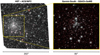 |
Fig. 1 Images of NGC 6558. Left: F606W/F814W combined colour image from the HST ACS/WFC camera for NGC 6558 (202 × 202 arcsec2). The green square represents the FoV of GSAOI (85 × 85 arcsec2). Right: J/KS combined colour image from the Gemini GSAOI camera. North is at the top and east is to the left for both images. |
2.2 Membership probability
The membership probability for each star was derived using the HST proper motions, right ascension (RA) and declination (Dec) values. We fitted a double Gaussian in each dimension of the vector-point diagram (VPD) to find the peak of the cluster distribution and the contribution of the high-spread background. Each star was assigned a Gaussian probability using the cluster mean and standard deviation in the proper motion distribution (top left panel of Figure 2). Since some background and foreground stars can have similar proper motions to the cluster and be wrongly assigned as members, we also combined the proper motion membership with a membership probability concerning the distance from the cluster centre (bottom left panel of Figure 2). The top middle panel shows the membership probability for the HST catalog. We assume that all stars with probabilities above 80% are cluster members. To remove the outlier stars that survived the membership selection, we performed some steps of the method applied by Maia et al. (2010) and briefly described as follows (bottom middle panel of Figure 2). In the same sky region, a sample of field and cluster stars were selected; here, we adopted stars with probabilities between 10% and 20% as the field reference, and probabilities above 80% as cluster members. The CMD was divided into a grid with Δ = 0.08 and Δ = 0.25 mag in colour and magnitude, respectively, which are equivalent to three times the standard deviation in colour and six times the standard deviation in magnitude. The density of field and cluster points in each cell were then compared. A probability was assigned for each cell as P = (Ncluster − Nfield)/Ncluster (equal to 0 when the numbr of field stars is larger than the cluster stars and removing cells with only one cluster star). In our case, this method was applied to remove as many outlier stars as possible. Therefore, the reference field must not be highly populated. The final CMD in the right panel of Figure 2 appears less contaminated after the cleaning method. The combined GSAOI+HST catalog was then obtained by cross-matching both catalogs.
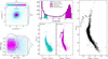 |
Fig. 2 Membership probability derivation. The top left and bottom left panels show the VPD and spatial position from the cluster centre coloured by the membership probability value. The upper corner and right panels show the double Gaussian fitting to the distributions. The top middle panel shows the membership distribution before (red) and after (blue) the cleaning method. The cyan region shows the membership range of reference field stars, while the magenta one is the cluster member probability region. The bottom middle panels show the reference field and cluster stars on the left and right, respectively. The cleaned CMD is shown in the right panel. The red star symbols show the OGLE RR Lyrae classified as members following the membership method. |
2.3 Differential reddening correction
We corrected the data from differential reddening using the method commonly applied in the literature (Piotto et al. 1999; Alonso-García et al. 2012; Milone et al. 2012; Hendricks et al. 2012; Bellini et al. 2017) and briefly described as follows. A sample of reference stars was selected, sometimes between the magnitudes where the angle between the reddening vector and the CMD is higher. A fiducial line was derived from this selection of stars. The distance of each reference star and the fiducial line was measured along the reddening vector. This distance was translated into the reddening of each reference star. In the final step, for each star in the catalogue, a number of neighbouring stars in the reference sample were selected; the final reddening of the specific star is the median of the reddening distribution of the neighbours. Some authors perform the method several times until the variation in the fiducial line becomes negligible. The differential reddening correction aims to reduce the spread along the CMD, bringing the stars as close as possible to the fiducial line. Therefore, creating the fiducial line is a crucial step for the differential reddening correction.
We derived the fiducial line in two different situations to show its influence on the final result of the differential reddening correction (Figure 3). First, we selected reference stars in the final combined GSAOI+ACS catalog, which is limited to the GSAOI FoV of 85 × 85 arcsec2 (left panels of Figure 3). In this representation, cyan dots denote field stars, while magenta dots represent cluster stars, consistent with Figure 2. Since the half-light radius of the cluster is ~45.1 arcsec (Baumgardt et al. 2020), the GSAOI FoV has more cluster members as field stars, which is reflected in our selection of reference stars, in which we have 7% of field stars (left panels of Figure 3). The differential reddening map obtained from this less contaminated selection is shown in the bottom left panel of Figure 3. In this work, we call this differential reddening correction from fiducial line 1 ‘DRCFL1’.
In another test, we selected the reference stars in the entire ACS/WFC FoV (middle panels of Figure 3). Since the centre of the cluster is imaged in one of the two ACS/WFC chips (see Figure 1), the ACS/WFC images cover a large portion of the field outside the half-light radius of the cluster, and thus more field stars are present in our catalog. Indeed, for this reference sample, we have 43% of field stars. We corrected for the effects of the differential reddening as before and obtained the map shown in the bottom middle panel of Figure 3. For a direct comparison with the previous test, DRCFL1, the panel only shows the same region covered by the GSAOI observations. We refer to this differential reddening correction from fiducial line 2 as ‘DRCFL2’.
A similar approach to DRCFL2 was used by Alonso-García et al. (2012) for NGC 6558, from observations in the B, V, and I bands obtained with the Magellan 6.5 m Telescope and the HST. They covered a circular area with a radius of approximately 217 arcsecs from the centre of the cluster, covering almost the same area as ACS/WFC FoV. Their resulting differential reddening map is shown in Figure 4. For a direct comparison, the three differential reddening maps cover the same area (GSAOI FoV) and have the same colour scale.
Both DRCFL1 and DRCFL2 maps show a consistent general behaviour, as was observed in Alonso-García et al. (2012): the southern region of the cluster exhibits positive differential reddening, whereas the northern one experiences negative differential reddening. Nevertheless, a systematic variation of approximately +0.05 mag is observed in the differential reddening when utilising GSAOI FoV stars (DRCFL1). This discrepancy arises from a 0.05 mag difference in the turn-off (TO) colour between the two fiducial lines, where the TO of fiducial line 2 is 0.05 magnitudes redder than the TO of fiducial line 2. The direct comparison of the resulting CMD using DRCFL1 (blue) and DRCFL2 (red) is shown in the right panel of Figure 3. This visualisation underscores the pivotal role of the fiducial line, particularly for clusters located within the galactic disc or projected towards the Galactic bulge, where the density of background stars is significantly higher, making the fiducial line redder.
For the subsequent analysis, we adopt the NGC 6558 results obtained by employing the DRCFL1, which takes into account less field star contamination in the differential reddening correction procedure. Nevertheless, we compare them with the results using the DRCFL2 to emphasise the possible biases resulting from the contamination by background field stars on the fiducial line creation. Figure 5 shows the three CMDs that are employed in this work: GSAOI [J, J −KS] (left panel), and HST/ACS [mF606W, mF606W − mF814W] using DRCFL1 (middle panel) and using DRCFL2 (right panel).
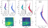 |
Fig. 3 Differential reddening correction procedure. The top left panels show the CMDs with the selected reference stars (the field as cyan dots and cluster as magenta dots, the same as in Figure 2) to generate the fiducial line (black line, left) and the corrected CMD (right). The differential reddening maps are at the bottom with respect to the cluster centre. Both density maps have the same colour code and scale and are limited to the GSAOI FoV. In the left panel is shown the differential reddening correction using the fiducial line constructed from the sample within the GSAOI FoV (DRCFL1), and in the middle panel the differential reddening correction using the fiducial line constructed from stars within the HST/ACS FoV. The right panel directly compares the cluster member stars using DRCFL1 (blue) and DRCFL2 (red). |
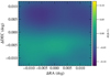 |
Fig. 4 Differential reddening map for NGC 6558 by Alonso-García et al. (2012). The density map has the same colour code, colour scale, and region as Figure 3. |
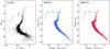 |
Fig. 5 Final CMDs with selected cluster members. The left panel is the GSAOI [KS, J − KS] CMD. The middle and right panels show the HST/ACS [mF606W, mF606W − mF814W] employing DRCFL1 and DRCFL2, respectively. The green star symbols are the RR Lyrae members of the cluster within the GSAOI FoV. |
3 RR Lyrae magnitude level
RR Lyrae stars from Clement et al. (2001) and OGLE-IV (Soszyński et al. 2014) databases were used, as in Oliveira et al. (2022), in order to provide a prior distribution to the cluster distance. Clement et al. (2001, updated in Apr 2016) contains 11 RR Lyrae with periods, amplitudes, and mean magnitudes in the I band, with a note that all the data comes from OGLE-IV in this case. Soszyński et al. (2014) lists seven RR Lyrae within a radius of 2.1′, but a wider search of 10′ in the OGLE Collection of Variable Stars1 returns 22 RR Lyrae, with the 11 more central ones in common with Clement et al. (2001). The latter provided timeseries photometry and mean I magnitudes from ∼660 epochs, and additional mean V magnitudes from 42 epochs.
A cross-match with our HST/ACS catalog retrieved five of the 22 RR Lyrae with a membership probability (derived in Section 2.2) higher than 80%, of which three are within the GSAOI FoV. A weighted average of the mean RR Lyrae magnitudes was obtained with membership values as weights, as is presented in Table 1 for the different filters. Figure 6 presents the mean V and I magnitudes as a function of the period.
The derived magnitudes were converted to the distance modulus in each iteration of the isochrone fitting using the MI - and MV − [Fe/H] relations from Oliveira et al. (2022) obtained with BaSTI α-enhanced models (Pietrinferni et al. 2021) for the zero-age horizontal branch, providing a variable prior in distance that varies with the reddening and metallicity of each Markov chain Monte Carlo (McMC) iteration. The use of the magnitude level appears to be a better constraint on the distance because the assumed metallicity, reddening, and RV play a key role in the final distance. For example, assuming a metallicity of [Fe/H] = −1.17 ± 0.10 (Barbuy et al. 2018b), the calibrations provide apparent distance moduli of (m − M)I = 15.30 ± 0.10 and (m − M)V = 15.86 ± 0.11. Converting them to absolute distance moduli using E(B − V) = 0.38 ± 0.05 mag from Barbuy et al. (2018b), the distances of 8.47 ± 0.52 and 8.63 ± 0.73 kpc were obtained, respectively, from I and V, whereas distances 0.4– 0.7 kpc smaller were derived with E(B − V) = 0.44 mag from Harris (1996, 2010 edition). All values were obtained assuming RV = 3.1. Therefore, by keeping the prior on the magnitude value of the RR Lyrae, we have avoided an erroneous distance determination to the detriment of some specific set of metallicity, reddening, and RV.
Oosterhoff (1939, 1944) classified the MW GCs into two classes based on the mean of the pulsation periods of their RR Lyrae stars: Oosterhoff type I (OoI) and Oosterhoff type II (OoII). In a nutshell (see also Prudil et al. 2019a,b; Martínez-Vázquez et al. 2021), OoI GCs have metallicity values above −1.7 and contain mainly RRab stars with a short average pulsation period of around 0.55 day. The OoI GCs also present a low fraction (∼20%) of RRc type RR Lyrae. In turn, OoII GCs contain a significant number of RRc stars (∼40%) and are more metal-poor than −1.7, and their RRab RR Lyrae sample shows an average pulsation period of ∼0.65 day. The mean period of RRab stars of NGC 6558 is 0.61 ± 0.04 days (Table 1). Even though the number of RR Lyrae stars selected as members of the cluster is low, we can estimate that the sample has 20% of first-overtone pulsators (RRc). The average period of RRab and number of RRc in our sample, together with the cluster metallicity of −1.18, could indicate that NGC 6558 is a OoI GC. Nevertheless, taking into account the low statistics, the average period of RRab stars could also point to the OoII type if the number of RRc stars were to increase with more observations.
Parameters of five RR Lyrae classified as members of NGC 6558 from their membership probabilities.
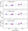 |
Fig. 6 Mean I, V, and G magnitudes versus the period of the RR Lyrae sample. The dashed lines mark the weighted average given in Table 1 and the dotted lines show the standard error. |
4 Isochrone fitting
The fundamental parameters – age, metallicity, distance, reddening, the total-to-selective extinction ratio, RV, and the binary fraction – were derived using the SIRIUS code (Souza et al. 2020). The code employs the Bayesian method of McMC to obtain probability distributions for each parameter. The code compares the observed CMD with synthetic CMDs constructed from each set of parameters randomly drawn during the fitting process.
To construct the synthetic diagrams, SIRIUS utilises isochrones from the Dartmouth Stellar Evolution Database (DSED; Dotter et al. 2008), which initially spans ages between 10 Gyr and 15 Gyr with intervals of 0.1 Gyr and metallicities between −2.30 and 0.0 with intervals of 0.01 dex. However, the code interpolates different isochrones during the fitting process to obtain the model with exact values. With the model constructed, the code adopts the initial mass function of Chabrier (2003) to draw N mass values. These values are then interpolated to obtain the corresponding magnitude values.
A fraction of these N mass values are associated with spatially unresolved photometric binary stars (stars close enough to have their flux overestimated). While the first star has mass mA, the hypothetical secondary star will have mass mB calculated as mB = q⋅mA, where q is the mass ratio randomly selected between 0 and 1. The calculation of the final magnitude of binary stars is computed from the sum of the flux of each star:
 (1)
(1)
With the magnitudes of each star calculated, an error function is applied to spread the points in the CMD. The error function is derived from the observed data by calculating the median error in magnitude bins. The error function is shifted to the position of the theoretical isochrone from the TO point to ensure no bias in the position of the synthetic diagram relative to the observed one. Thus, whatever set of parameters is drawn, the error function will generate a synthetic CMD.
After spreading the stars according to the error function, the code calculates the extinction coefficients following the extinction law (RV) of each iteration. The extinction law is interpolated from the curves of Cardelli et al. (1989), and the extinction coefficients for the J, KS, F606W, and F814W bands are obtained from this. Then, each absolute magnitude is converted to the apparent magnitude as follows:
 (2)
(2)
where (m − M)0 is the intrinsic distance modulus, and Aλ is the extinction coefficient in band λ.
With the synthetic diagram already containing the apparent magnitudes, a luminosity function is applied to reproduce the observation conditions to which the data were subjected. The luminosity function is calculated as the number of stars in each magnitude bin. When applied to the synthetic diagram, some stars will be excluded to make the synthetic diagram more similar to the observed one in terms of the number of stars at each magnitude.
When the RV is a free parameter, the isochrone fitting is performed simultaneously for the [J, J−KS] and [mF606W, mF606W − mF814W] diagrams. Simultaneous fitting allows the determination of the extinction law, since it will force the adjustment of a single set of distance and reddening for the two diagrams. Another advantage of this approach is that the age determination is not biased by the choice of photometric system.
As a proxy for distance, we employed a prior to the distance according to the magnitude level of RR Lyrae stars. For each McMC interaction, the values of metallicity and reddening were used for the MI − [Fe/H] calibration by Oliveira et al. (2022),
![${M_I} = A + B \cdot [{\rm{Fe}}/{\rm{H}}] + C \cdot {[{\rm{Fe}}/{\rm{H}}]^2},$](/articles/aa/full_html/2024/10/aa50795-24/aa50795-24-eq5.png) (3)
(3)
where A = (0.619 ± 0.028), B = (0.455 ± 0.063), and C = (0.075 ± 0.030). Then, the expected distance for the previously RR Lyrae magnitude level, reddening, and metallicity was calculated for each interaction. This calculated distance was then compared with the distance value for the specific McMC interaction.
The McMC was applied using the Python library, emcee (Foreman-Mackey et al. 2013), and PyDE2, a global optimisation that uses differential evolution. The likelihood function is an adaptation of Tremmel et al. (2013), which is basically a Poisson distribution comparing the number of observed and synthetic stars in a colour and magnitude bin. The adaptation includes a simple isochrone fitting component comparing the isochrone to the two-dimensional distribution of observed points. This change allows the code to reach the stability of the distance and reddening values more quickly. Meanwhile, the likelihood component that compares the synthetic diagram with the observed one allows for a better age and binary fraction calculation.
In the isochrone fitting procedure below, we applied the metallicity from Barbuy et al. (2018a) and the RR Lyrae magnitude level from Section 3 as priors. Figures 7 and 8 show the simultaneous isochrone fitting on the [J, J − KS] and the [mF606W, mF606W − mF814W] CMDs (the corner plots are shown in Figure A.1). Figure 7 shows the HST CMD with the DRCFL1 and Figure 8 adopting DRCFL2. The distance values, d⊙ = 8.41 ± 0.10 and 8.44 ± 0.10 kpc, respectively, are in excellent agreement between each other. This agreement is, however, due to compensation in the reddening value, E(B − V), and the extinction law, RV, parameter. The E(B − V) values are 0.34 ± 0.02 and 0.42 ± 0.02 for DRCFL1 and DRCFL2, respectively. More important is the difference in the RV values of 3.2 and 2.9. The low RV was expected because the data of DRCFL2 include background Galactic bulge field stars that are affected by dust (Minniti et al. 2014; Nataf 2016). Removing the Galactic bulge field stars, as in the case of DRCFL1, the relatively high RV = 3.2 is compatible with the Galactic latitude of NGC 6558 (l = −6.02°), which is outside the dark lane region (Minniti et al. 2014; Nataf 2016). Finally, the difference in the derived ages, 13.0 ± 0.9 and 13.4 ± 0.8 Gyr, reflects the different morphology of the respective fiducial line and the difference in the MSTO colour (~0.05 mag).
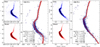 |
Fig. 7 Simultaneous isochrone fitting using the differential reddening correction from fiducial line 1 (DRCFL1). The left panels show the NIR GSAOI CMD and the right panels show the optical F606W/F814W HST CMD. The small panels show the Hess diagram of the data (upper) and model (best-fit synthetic CMD, lower). In the bigger panel, the blue dots are the cluster member stars, the red line represents the isochrone of the best synthetic CMD fit, and the thin lines are solutions within the errors. The values obtained from the simultaneous fitting are shown in the bottom left corner of the bigger panels, with the respective binary fraction value highlighted. |
5 Orbital parameters
We performed the orbital integration of NGC 6558 in order to derive the orbital parameters: the apogalactic distance (< rapo >) and perigalactic distance (< rperi >), eccentricity (ecc = (< rapo > − < rperi >)/(< rapo > + < rperi >)), and the maximum absolute height relative to the disc (< |Z|max >). For the orbital integration, we adopted the MW model from Portail et al. (2017) by using the analytical approximation given by Sormani et al. (2022) with the Action-based GAlaxy Modelling Architecture (AGAMA; Vasiliev 2019), a Python package for orbital integration3. The Galactic model of Portail et al. (2017) is composed of the x-shape peanut or bulge bar, a long bar, a central concentration mass, a disc, and a dark-matter halo. This Galactic model describes the complexity of the inner Galactic region (within ~5 kpc) well, although further out it is not very realistic. In the case of NGC 6558, this potential is the most suitable, since this cluster is supposed to belong to the Galactic bulge (Bica et al. 2016; Pérez-Villegas et al. 2018, 2020).
In this model, the position of the Sun is at a distance of R0 = 8.2 kpc (Bland-Hawthorn & Gerhard 2016) from the Galactic centre. The bar rotates with a pattern speed of 39 km s−1 kpc−1 and is oriented at an angle of 28° with the Sun–Galactic centre line of sight. The mass distribution of the model has a local circular velocity of V(R0) = 239.2 km s−1. The peculiar motion of the Sun with respect to the local circular orbit is (U0, V0, W0)=(11.1, 12.24, 7.25) km s−1 (Schönrich et al. 2010).
The observational parameters RA, Dec, radial velocity, distance from the Sun, and proper motions in the sky of the cluster, presented in the upper part of Table 2, were converted to Cartesian Galactic phase-space positions and velocities using the Astropy Python package (Astropy Collaboration 2022). To take into account the uncertainties of the observational parameters, we constructed 1000 initial conditions using the Monte Carlo approach, and integrated the orbits backwards in time for 13 Gyr. The median orbital parameters and the probabilities of belonging to the Galactic bulge and following the bar orbit are shown in the bottom part of Table 2. From the values of the apocentric distance, < rapo >, and maximum height, < |Z|max >, together with the classification criteria of Pérez-Villegas et al. (2020), NGC 6558 currently has a 99% probability of belonging to the early Galactic bulge. Our results are in good agreement with the calculations given in Pérez-Villegas et al. (2020). Figure 9 shows the density probability map of the orbits of NGC 6558 in the x−y (upper left), R−y (upper right), x−z (bottom left), and R−z (bottom right) projections. The space region in which the orbits of NGC 6558 cross more frequently is shown in orange. The black curves are the orbits considering the central values of the observational parameters. Regarding the sense of the orbital motion, we found that for NGC 6558 it is prograde and retrograde at the same time. The prograde–retrograde orbits, which have been observed in other MW GCs too, are produced by the presence of the Galactic bar; this behaviour could be connected with chaos, but is still not yet well understood (Pichardo et al. 2004; Allen et al. 2006; Pérez-Villegas et al. 2018).
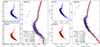 |
Fig. 8 Same as in Figure 7 but using the differential reddening correction from fiducial line 2 (DRCFL2). |
Observational parameters used as input to the orbital integration.
6 Discussion
For the following discussion, we adopted the isochrone fitting results of DRCFL1 as the final parameters for NGC 6558. In Table 3, we tentatively identify a list of Galactic bulge clusters with characteristics similar to NGC 6558, which are probably the oldest objects in the Galaxy. A list of possible members is also given for clusters that still do not have precise age derivation and/or were classified as thick disc members by PV20. It is important to point out that the classification as a bulge or thick disc member depends crucially on the distance adopted, which may be uncertain with the available data. A summary of the literature data for NGC 6558, including reddening values, age, distance, the corresponding method employed, and metallicity, is given in Table 4.
The metallicities derived from the isochrone fitting are in good agreement with the value from Barbuy et al. (2018a); González-Díaz et al. (2023), since it was adopted as a prior. The metallicity of NGC 6558 was therefore consolidated from literature studies, as follows. Barbuy et al. (2007) carried out a detailed abundance analysis of five stars with spectra obtained with the GIRAFFE spectrograph at the Very Large Telescope (VLT) (see also Zoccali et al. 2008). They obtained a mean metallicity of [Fe/H]= −0.97 ± 0.15 for NGC 6558. From CaT triplet lines based on FORS2/VLT spectra, Saviane et al. (2012) derived [Fe/H]= −1.03 ± 0.14. Also based on FORS2/VLT spectra, Dias et al. (2015, 2016) compared the observed spectra to grids of observed and synthetic spectra and obtained [Fe/H]= −1.012 ± 0.013. Barbuy et al. (2018b) analysed four stars of NGC 6558 observed with the UVES spectrograph at the VLT. A radial velocity of 194.45 km s−1 and metallicity of [Fe/H]= −1.17 ± 0.10 were obtained. González-Díaz et al. (2023) analysed four stars within the APOGEE-2S CNTAC 2 CN2019B programme (P.I: Doug Geisler) as part of the CAPOS survey (Geisler et al. 2021). They obtained a radial velocity of 192.63 km s−1 and a metallicity of [Fe/H]= −1.15 ± 0.10.
Therefore, the Gaussian metallicity prior with a mean of -1.17 and standard deviation of 0.10 is reasonable to encompass the literature metallicity derivations.
The derived heliocentric distance of the cluster, d⊙ =  kpc, is larger than other data given in the literature. Rich et al. (1998) observed NGC 6558 with the New Technology Telescope (NTT) at the European Southern Observatory using the ESO Multi-Mode Instrument (EMMI) in the imaging/focal reducer mode, reaching a magnitude of V∼20.5 in the CMD. They derived a lower distance of 6.3 kpc and metallicity between [Fe/H]= −1.2 to −1.6. Baumgardt & Vasiliev (2021) also found a lower distance of d⊙ = 7.47 kpc, taking the average distance determinations in the literature, which is in agreement with d⊙ = 7.4 ± 0.7 kpc from Rossi et al. (2015) who used two-epoch NTT data. A larger distance of d⊙ = 8.26 kpc close to our determination was given in Barbuy et al. (2018b), derived from proper-motion-cleaned NTT photometry, in [V, V − I].
An important contribution of this work is the simultaneous isochrone fitting using both the NIR and optical photometries. This approach enables the total-to-selective coefficient, RV (e.g. Pallanca et al. 2021), to be determined by imposing one set of fundamental parameters to fit both CMDs. With DRCFL1, we derived RV = 3.2 ± 0.2, and using DRCFL2, we derived RV = 2.8 ± 0.1. The lower value obtained with DRCFL2 reflects the presence of stars in the dust dark lane (Minniti et al. 2014) given that there is a larger contribution from field stars in the HST FoV (Figure 1). The variation in the RV value also implies a reddening E(B − V) value variation. In Table 4, the reddening E(B − V) literature values range from 0.38 to 0.50. Interestingly, the isochrone fitting gives the values E(B − V)= 0.34 ± 0.02 and 0.42 ± 0.02 for DRCFL1 and DRCFL2, respectively. This variation again shows that the reddening tends to decrease to the value of E(B − V)= 0.35 when removing the background Galactic bulge field stars behind the dust lane. The reddening in infrared bands E(J − KS) can be obtained from the E(B − V) and RV provided by our results using the following equation: E(J − KS) = E(B − V) ⋅ RV ⋅  . For RV = 3.24 (our result), RJ = 0.29186045 and
  . Therefore, E(J − KS) = 0.34 ⋅ 3.24 ⋅ (0.29186045 − 0.11886802) = 0.19. The extinction in each band is obtained from AJ = RJ ⋅ E(B − V)·RV = 0.29186045 ⋅ 0.34 ⋅ 3.24 = 0.32.
The age determination also differs according to the adopted DRCFL1 or DRCFL2, with values of 13.0 ± 0.9 and 13.4 ± 0.9 Gyr, respectively. There is a trend towards older ages with DRCFL2 because of the higher contamination of Galactic bulge field stars. This interesting trend indicates that the Galactic bulge is even older than NGC 6558. Cohen et al. (2021), using the method of relative age, derived an age of 12.3 ± 1.1 Gyr for NGC 6558. They used the same observations as those used in this work, which were reduced with a different pipeline. The values derived in this work and by Cohen et al. (2021) agree within the errors, even though the median values differ by 0.7 Gyr.
To insert the results of this work in the context of the Galactic bulge formation, we analysed the sample of moderately metal-poor (MMP, [Fe/H] ∼ −1.10) GCs of the Galactic bulge, which have available age determination in the literature (Table 3). We selected the orbital parameters of the clusters from Pérez-Villegas et al. (2020), while for NGC 6558 we considered only the results from the present DRCFL1 (Table 2).
In the left panel of Figure 10 is the ecc versus |Z|max plane divided into nine cells named from A to I. This plane is a very good way to split as much as possible the different populations of the inner Galaxy (Queiroz et al. 2021). The important cells for this work are those with high eccentricity because their shapes are supported by pressure, indicating a spheroidal structure. Razera et al. (2022) analysed a sample of 58 stars from the reduced-proper-motion (RPM) sample of the inner Galaxy (Queiroz et al. 2021) with metallicity values around the peak of the Galactic bulge metallicity distribution function (∼ −1.1; Bica et al. 2016). These stars are shown in the left panel of Figure 10 as cyan squares. After a meticulous chemical analysis, the authors concluded that this star sample is a genuine member of a spheroidal structure in the inner Galaxy. The MMP GCs are all located in cells C and F, indicating that they are also possible members of the spheroidal Galactic bulge. Moreover, since all MMP GCs are located in cell F, this cell probably represents the oldest population of the inner Galaxy.
In principle, the AMR of the Galactic bulge MMP GCs shows they are almost coeval among them (right panel of Figure 10). The grey dots in the right panel of Figure 10 represent the sample of 96 Galactic GCs collected by Kruijssen et al. (2019). The authors provide an average age for all GCs using the three by Forbes & Bridges (2010), Dotter et al. (2010, 2011), and VandenBerg et al. (2013). In order to investigate the old and spheroidal structure of the inner Galaxy (cell F), we fitted the AMR for the MMP GCs using the leaky-box formalism often used in the literature (e.g. Massari et al. 2019; Forbes 2020; Limberg et al. 2022; Callingham et al. 2022), with some modifications:
![$Z = - \rho \cdot \ln \left( {{t \over {{t_f}}}} \right) = {Z_ \odot } \cdot {10^{[{\rm{M}}/{\rm{H}}]}},$](/articles/aa/full_html/2024/10/aa50795-24/aa50795-24-eq11.png) (4)
(4)
where tf is the look-back time at which the stellar population starts to form stars, Z⊙ = 0.019 for the solar total metallicity, and ρ is the effective yield of the stellar population. ρ represents the mass ratio of the new stars formed from the enriched gas expelled from supernovae, and is therefore a measure of the chemical enrichment efficiency of the stellar population and is in units of solar total metallicity (Z⊙). We considered the relation [M/H] = [Fe/H] + log10 (0.694 ⋅ 10[α/Fe] + 0.306). For the MMP GCs of the Galactic bulge, we assumed [α/Fe] = +0.4 (Barbuy et al. 2018a) and [α/Fe] = +0.0 for the ex situ GCs (Helmi et al. 2018) Therefore:
![$t = {t_f} \cdot \exp \left( { - {{{Z_ \odot }} \over \rho } \cdot {{10}^{[{\rm{Fe}}/{\rm{H}}] + \Delta }}} \right)\left\{ {\matrix{ {\Delta = 0.312} \hfill & {{\rm{ for MMPGCs }}} \hfill \cr {\Delta = 0.0} \hfill & {{\rm{ for ex situ GCs }}} \hfill \cr } } \right.{\rm{. }}$](/articles/aa/full_html/2024/10/aa50795-24/aa50795-24-eq12.png) (5)
(5)
For the MMP GC Galactic bulge population (Table 3), we obtained a yield of ρ = 0.051 ± 0.014 Z⊙ and tf = 13.623 ± 0.196 Gyr. The derived tf value indicates that this population is among the oldest in the Galaxy, since its formation time is close to the age of the Universe of 13.799 ± 0.021 Gyr (Planck Collaboration XIII 2016). To investigate the derived effective yield, we also fitted the ex situ branch of the AMR. The result is the solid cyan line in the right panel of Figure 10 with ρ = 0.007 ± 0.009 Z⊙ and tf = 13.083 ± 0.124 Gyr. The effective yield is approximately eight times smaller than the value derived for the MMP GCs. In the right panel of Figure 10, we also present as a dashed red line the AMR with an effective yield ten times smaller than the MMP GCs and with the same tf. It indicates that the spheroidal structure of the inner Galaxy represented by cell F was formed at the beginning of the Galaxy 13.623 ± 0.196 Gyr ago and has been chemically enriched approximately ten times faster than the rest of the Galaxy (Barbuy et al. 2018a).
Family of Galactic bulge GCs with a metallicity of [Fe/H]∼−1.1, and very old age.
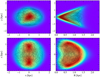 |
Fig. 9 Density probability map for the x–y (upper left), R−y (upper right), x−z (bottom left), and R−z (bottom right) projections of the set of orbits for NGC 6558. Orange corresponds to higher probabilities. The black lines show the orbits using the main observational parameters. |
Literature ages and metallicities for NGC 6558.
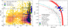 |
Fig. 10 Analysis of the moderately metal-poor side of the Galactic bulge GCs. Left panel: ecc vs. |Z|max plane divided into nine regions named from A to I. The background density map shows the RPM sample (Queiroz et al. 2021): the blue dots are the MMP GCs, and the cyan squares are the 58 Galactic bulge spheroid stars from Razera et al. (2022). NGC 6558 is the green star symbo (see Pérez-Villegas et al. 2020; Queiroz et al. 2021; Razera et al. 2022 for the orbital parameter calculations). Right panel: Derivation of the AMR (red line) for the sample of GCs in Table 3 (blue dots). The thin red lines correspond to the AMR varying the mean parameters within errors. The dashed red line shows the AMR assuming a chemical enhancement ten times slower than the one derived for the MMPGCs, while the cyan line is the AMR fitted to the ex situ GCs. |
7 Conclusions
We have used high-quality photometric data from Gemini-South/GSAOI and HST/ACS to derive the parameters of distance, reddening, the total-to-selective coefficient, and age for the Galactic bulge GC NGC 6558. For the isochrone fitting, the metallicity from high-resolution spectroscopy and the apparent magnitude level of RR Lyrae were adopted as priors.
We demonstrated the importance of the adopted sample of stars in determining the fiducial line for the differential reddening correction. In the NGC 6558 case, in which background Galactic bulge field stars contaminate the sample, the isochrone fitting results in a lower RV and higher extinction, compatible with including Galactic bulge field stars behind a dust lane. Contrarily, removing the Galactic bulge field stars, the results are more compatible with the Galactic latitude of the cluster. The combination of NIR and optical data allowed the total-to-selective coefficient to be estimated as RV = 3.2 ± 0.2 once a fiducial line based on cluster stars with a smaller contribution of field stars was adopted.
The distance of  kpc obtained is farther than any other such distance in the literature, exemplifying the difficulties of deriving distance values, even in the Gaia era, due to the high reddening in the Galactic bulge (see also Vasiliev & Baumgardt 2021). The reddening of E(B − V)= 0.34 ± 0.02 is the lowest value relative to the literature, obtained with the differential reddening correction based on reference stars that are less contaminated by field stars. The age of 13.0±0.9 Gyr obtained is compatible with the similarly MMP Galactic bulge clusters listed in Table 3.
Finally, combining NGC 6558 with the other MMP GCs of the Galactic bulge located within the spheroidal inner structure (cell F in ecc vs. |Z|max plane), we obtained a steep asymptotic trend, indicating that the formation time of this population is as late as 13.62 Gyr and that it has a chemical enrichment ten times faster than the rest of the MW, making clear that this family of clusters includes the oldest objects in the Galaxy.
Acknowledgements
The authors are grateful to the anonymous referee for his/her suggestions and remarks, which greatly improved the paper. SOS acknowledges a FAPESP PhD fellowship no. 2018/22044-3. A.P.V. and S.O.S acknowledge the DGAPA–PAPIIT grant IA103224. SO acknowledges the support of the University of Padova, DOR Ortolani 2020, Piotto 2021 and Piotto 2022, Italy and funded by the European Union – NextGenerationEU" RRF M4C2 1.1 no.: 2022HY2NSX. “CHRONOS: adjusting the clock(s) to unveil the CHRONOchemo-dynamical Structure of the Galaxy” (PI: S. Cassisi). BB and EB acknowledge partial financial support from FAPESP, CNPq and CAPES – Financial code 001. B.D. acknowledges support by ANID-FONDECYT iniciación grant No. 11221366 and from the ANID Basal project FB210003. L.O.K. acknowledges partial financial support by CNPq (proc. 313843/2021-0) and UESC (proc. 073.6766.2019.0013905-48). This research is based on observations made with the NASA/ESA Hubble Space Telescope obtained from the Space Telescope Science Institute, which is operated by the Association of Universities for Research in Astronomy, Inc., under NASA contract NAS 5–26555. The HST observations are associated with programmes GO-9799 (PI: Rich) and GO-15065 (PI: Cohen). Based on observations obtained at the international Gemini Observatory, a programme of NSF NOIRLab, which is managed by the Association of Universities for Research in Astronomy (AURA) under a cooperative agreement with the U.S. National Science Foundation on behalf of the Gemini Observatory partnership: the U.S. National Science Foundation (United States), National Research Council (Canada), Agencia Nacional de Investigación y Desarrollo (Chile), Ministerio de Ciencia, Tecnología e Innovación (Argentina), Ministério da Ciência, Tecnologia, Inovações e Comunicações (Brazil), and Korea Astronomy and Space Science Institute (Republic of Korea). The Gemini observations are associated with the programme GS-2020A-Q-121 (PI: L. Kerber).
Appendix A Corner-plots
In this section we show the corner-plots for the simultaneous isochrone fitting. The binary fractions are different for each CMD: na for the NIR and nb for the HST CMDs. In Figure A.1, the upper panel shows the results for DRCFL1 and bottom panel for DRCFL2. The corner-plots are an important diagnostical too to visualise the behaviour of the McMC and the correlations among the parameter as well.
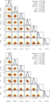 |
Fig. A.1 Corner-plots with the results for the isochrone fitting using DRCFL1 (upper panel) and DRCFL2 (bottom panel). The characteristic values are composed of the median and the 16 and 84 percentiles of the distributions. |
References
- Allen, C., Moreno, E., & Pichardo, B. 2006, ApJ, 652, 1150 [NASA ADS] [CrossRef] [Google Scholar]
- Alonso-García, J., Mateo, M., Sen, B., et al. 2012, AJ, 143, 70 [Google Scholar]
- Anderson, J., & van der Marel, R. P. 2010, ApJ, 710, 1032 [NASA ADS] [CrossRef] [Google Scholar]
- Astropy Collaboration (Price-Whelan, A. M., et al.) 2022, ApJ, 935, 167 [NASA ADS] [CrossRef] [Google Scholar]
- Barbuy, B., Zoccali, M., Ortolani, S., et al. 2007, AJ, 134, 1613 [Google Scholar]
- Barbuy, B., Cantelli, E., Vemado, A., et al. 2016, A&A, 591, A53 [NASA ADS] [CrossRef] [EDP Sciences] [Google Scholar]
- Barbuy, B., Chiappini, C., & Gerhard, O. 2018a, ARA&A, 56, 223 [NASA ADS] [CrossRef] [Google Scholar]
- Barbuy, B., Muniz, L., Ortolani, S., et al. 2018b, A&A, 619, A178 [NASA ADS] [CrossRef] [EDP Sciences] [Google Scholar]
- Barbuy, B., Cantelli, E., Muniz, L., et al. 2021a, A&A, 654, A29 [NASA ADS] [CrossRef] [EDP Sciences] [Google Scholar]
- Barbuy, B., Ernandes, H., Souza, S. O., et al. 2021b, A&A, 648, A16 [NASA ADS] [CrossRef] [EDP Sciences] [Google Scholar]
- Baumgardt, H., & Hilker, M. 2018, MNRAS, 478, 1520 [Google Scholar]
- Baumgardt, H., & Vasiliev, E. 2021, MNRAS, 505, 5957 [NASA ADS] [CrossRef] [Google Scholar]
- Baumgardt, H., Sollima, A., & Hilker, M. 2020, PASA, 37, e046 [Google Scholar]
- Bellini, A., Anderson, J., Bedin, L. R., et al. 2017, ApJ, 842, 6 [NASA ADS] [CrossRef] [Google Scholar]
- Belokurov, V., & Kravtsov, A. 2024, MNRAS, 528, 3198 [CrossRef] [Google Scholar]
- Belokurov, V., Erkal, D., Evans, N. W., Koposov, S. E., & Deason, A. J. 2018, MNRAS, 478, 611 [Google Scholar]
- Bica, E., Ortolani, S., & Barbuy, B. 2016, PASA, 33, e028 [Google Scholar]
- Bica, E., Ortolani, S., Barbuy, B., & Oliveira, R. A. P. 2024, A&A, 687, A201 [NASA ADS] [CrossRef] [EDP Sciences] [Google Scholar]
- Bland-Hawthorn, J., & Gerhard, O. 2016, ARA&A, 54, 529 [Google Scholar]
- Bovy, J., Leung, H. W., Hunt, J. A. S., et al. 2019, MNRAS, 490, 4740 [Google Scholar]
- Callingham, T. M., Cautun, M., Deason, A. J., et al. 2022, MNRAS, 513, 4107 [NASA ADS] [CrossRef] [Google Scholar]
- Cardelli, J. A., Clayton, G. C., & Mathis, J. S. 1989, ApJ, 345, 245 [Google Scholar]
- Carretta, E., Bragaglia, A., Gratton, R., D’Orazi, V., & Lucatello, S. 2009, A&A, 508, 695 [NASA ADS] [CrossRef] [EDP Sciences] [Google Scholar]
- Chabrier, G. 2003, PASP, 115, 763 [Google Scholar]
- Chun, S. H., Kim, J. W., Shin, I. G., et al. 2010, A&A, 518, A15 [NASA ADS] [CrossRef] [EDP Sciences] [Google Scholar]
- Clement, C. M., Muzzin, A., Dufton, Q., et al. 2001, AJ, 122, 2587 [NASA ADS] [CrossRef] [Google Scholar]
- Cohen, R. E., Bellini, A., Casagrande, L., et al. 2021, AJ, 162, 228 [NASA ADS] [CrossRef] [Google Scholar]
- Davidge, T. J., Ledlow, M., & Puxley, P. 2004, AJ, 128, 300 [NASA ADS] [CrossRef] [Google Scholar]
- Debattista, V. P., Ness, M., Gonzalez, O. A., et al. 2017, MNRAS, 469, 1587 [Google Scholar]
- Dias, B., Barbuy, B., Saviane, I., et al. 2015, A&A, 573, A13 [NASA ADS] [CrossRef] [EDP Sciences] [Google Scholar]
- Dias, B., Barbuy, B., Saviane, I., et al. 2016, A&A, 590, A9 [NASA ADS] [CrossRef] [EDP Sciences] [Google Scholar]
- Dotter, A., Chaboyer, B., Jevremovic´, D., et al. 2008, ApJS, 178, 89 [NASA ADS] [CrossRef] [Google Scholar]
- Dotter, A., Sarajedini, A., Anderson, J., et al. 2010, ApJ, 708, 698 [Google Scholar]
- Dotter, A., Sarajedini, A., & Anderson, J. 2011, ApJ, 738, 74 [NASA ADS] [CrossRef] [Google Scholar]
- Ernandes, H., Dias, B., Barbuy, B., et al. 2019, A&A, 632, A103 [EDP Sciences] [Google Scholar]
- Fernández-Trincado, J. G., Zamora, O., Souto, D., et al. 2019, A&A, 627, A178 [Google Scholar]
- Fernández-Trincado, J. G., Minniti, D., Beers, T. C., et al. 2020, A&A, 643, A145 [Google Scholar]
- Fernández-Trincado, J. G., Beers, T. C., Minniti, D., et al. 2021, A&A, 647, A64 [EDP Sciences] [Google Scholar]
- Forbes, D. A. 2020, MNRAS, 493, 847 [Google Scholar]
- Forbes, D. A., & Bridges, T. 2010, MNRAS, 404, 1203 [NASA ADS] [Google Scholar]
- Foreman-Mackey, D., Hogg, D. W., Lang, D., & Goodman, J. 2013, PASP, 125, 306 [Google Scholar]
- Fragkoudi, F., Grand, R. J. J., Pakmor, R., et al. 2020, MNRAS, 494, 5936 [Google Scholar]
- Gaia Collaboration (Brown, A. G. A., et al.) 2018a, A&A, 616, A1 [NASA ADS] [CrossRef] [EDP Sciences] [Google Scholar]
- Gaia Collaboration (Helmi, A., et al.) 2018b, A&A, 616, A12 [NASA ADS] [CrossRef] [EDP Sciences] [Google Scholar]
- Garro, E. R., Fernández-Trincado, J. G., Minniti, D., et al. 2023, A&A, 669, A136 [NASA ADS] [CrossRef] [EDP Sciences] [Google Scholar]
- Garro, E. R., Minniti, D., & Fernández-Trincado, J. G. 2024, A&A, 687, A214 [NASA ADS] [CrossRef] [EDP Sciences] [Google Scholar]
- Geisler, D., Villanova, S., O’Connell, J. E., et al. 2021, A&A, 652, A157 [NASA ADS] [CrossRef] [EDP Sciences] [Google Scholar]
- Geisler, D., Parisi, M. C., Dias, B., et al. 2023, A&A, 669, A115 [NASA ADS] [CrossRef] [EDP Sciences] [Google Scholar]
- González-Díaz, D., Fernández-Trincado, J. G., Villanova, S., et al. 2023, MNRAS, 526, 6274 [CrossRef] [Google Scholar]
- Harris, W. E. 1996, AJ, 112, 1487 [Google Scholar]
- Hazen, M. L. 1996, AJ, 111, 1184 [NASA ADS] [CrossRef] [Google Scholar]
- Helmi, A., Babusiaux, C., Koppelman, H. H., et al. 2018, Nature, 563, 85 [Google Scholar]
- Hendricks, B., Stetson, P. B., VandenBerg, D. A., & Dall’Ora, M. 2012, AJ, 144, 25 [NASA ADS] [CrossRef] [Google Scholar]
- Horta, D., Schiavon, R. P., Mackereth, J. T., et al. 2021, MNRAS, 500, 1385 [Google Scholar]
- Kerber, L. O., Nardiello, D., Ortolani, S., et al. 2018, ApJ, 853, 15 [Google Scholar]
- Kerber, L. O., Libralato, M., Souza, S. O., et al. 2019, MNRAS, 484, 5530 [Google Scholar]
- Kharchenko, N. V., Piskunov, A. E., Schilbach, E., Röser, S., & Scholz, R. D. 2016, A&A, 585, A101 [NASA ADS] [CrossRef] [EDP Sciences] [Google Scholar]
- Kruijssen, J. M. D., Pfeffer, J. L., Reina-Campos, M., Crain, R. A., & Bastian, N. 2019, MNRAS, 486, 3180 [Google Scholar]
- Kruijssen, J. M. D., Pfeffer, J. L., Chevance, M., et al. 2020, MNRAS, 498, 2472 [NASA ADS] [CrossRef] [Google Scholar]
- Libralato, M., Lennon, D. J., Bellini, A., et al. 2021, MNRAS, 500, 3213 [Google Scholar]
- Libralato, M., Bellini, A., Vesperini, E., et al. 2022, ApJ, 934, 150 [NASA ADS] [CrossRef] [Google Scholar]
- Limberg, G., Souza, S. O., Pérez-Villegas, A., et al. 2022, ApJ, 935, 109 [NASA ADS] [CrossRef] [Google Scholar]
- Maia, F. F. S., Corradi, W. J. B., & Santos, J. F. C., J. 2010, MNRAS, 407, 1875 [NASA ADS] [CrossRef] [Google Scholar]
- Martínez-Vázquez, C. E., Cerny, W., Vivas, A. K., et al. 2021, AJ, 162, 253 [CrossRef] [Google Scholar]
- Massari, D., Koppelman, H. H., & Helmi, A. 2019, A&A, 630, A4 [NASA ADS] [CrossRef] [EDP Sciences] [Google Scholar]
- McMillan, P. J. 2017, MNRAS, 465, 76 [NASA ADS] [CrossRef] [Google Scholar]
- Meissner, F., & Weiss, A. 2006, A&A, 456, 1085 [CrossRef] [EDP Sciences] [Google Scholar]
- Milone, A. P., Marino, A. F., Cassisi, S., et al. 2012, ApJ, 754, L34 [NASA ADS] [CrossRef] [Google Scholar]
- Minniti, D., Saito, R. K., Gonzalez, O. A., et al. 2014, A&A, 571, A91 [NASA ADS] [CrossRef] [EDP Sciences] [Google Scholar]
- Moreno, E., Fernández-Trincado, J. G., Pérez-Villegas, A., Chaves-Velasquez, L., & Schuster, W. J. 2022, MNRAS, 510, 5945 [NASA ADS] [CrossRef] [Google Scholar]
- Nardiello, D., Libralato, M., Piotto, G., et al. 2018, MNRAS, 481, 3382 [NASA ADS] [CrossRef] [Google Scholar]
- Nataf, D. M. 2016, PASA, 33, e024 [CrossRef] [Google Scholar]
- Nepal, S., Chiappini, C., Guiglion, G., et al. 2024, A&A, 681, A8 [Google Scholar]
- Nogueras-Lara, F., Feldmeier-Krause, A., Schödel, R., et al. 2023a, A&A, 680, A75 [NASA ADS] [CrossRef] [EDP Sciences] [Google Scholar]
- Nogueras-Lara, F., Schultheis, M., Najarro, F., et al. 2023b, A&A, 671, A10 [NASA ADS] [CrossRef] [EDP Sciences] [Google Scholar]
- Oliveira, R. A. P., Souza, S. O., Kerber, L. O., et al. 2020, ApJ, 891, 37 [Google Scholar]
- Oliveira, R. A. P., Ortolani, S., Barbuy, B., et al. 2022, A&A, 657, A123 [NASA ADS] [CrossRef] [EDP Sciences] [Google Scholar]
- Oosterhoff, P. T. 1939, The Observatory, 62, 104 [NASA ADS] [Google Scholar]
- Oosterhoff, P. T. 1944, Bull. Astron. Inst. Netherlands, 10, 55 [NASA ADS] [Google Scholar]
- Ortolani, S., Held, E. V., Nardiello, D., et al. 2019, A&A, 627, A145 [NASA ADS] [CrossRef] [EDP Sciences] [Google Scholar]
- Pallanca, C., Lanzoni, B., Ferraro, F. R., et al. 2021, ApJ, 913, 137 [NASA ADS] [CrossRef] [Google Scholar]
- Pérez-Villegas, A., Portail, M., & Gerhard, O. 2017, MNRAS, 464, L80 [CrossRef] [Google Scholar]
- Pérez-Villegas, A., Rossi, L., Ortolani, S., et al. 2018, PASA, 35, e021 [CrossRef] [Google Scholar]
- Pérez-Villegas, A., Barbuy, B., Kerber, L. O., et al. 2020, MNRAS, 491, 3251 [Google Scholar]
- Pichardo, B., Martos, M., & Moreno, E. 2004, ApJ, 609, 144 [NASA ADS] [CrossRef] [Google Scholar]
- Pietrinferni, A., Hidalgo, S., Cassisi, S., et al. 2021, ApJ, 908, 102 [NASA ADS] [CrossRef] [Google Scholar]
- Pinna, F., Walo-Martín, D., Grand, R. J. J., et al. 2024, A&A, 683, A236 [NASA ADS] [CrossRef] [EDP Sciences] [Google Scholar]
- Piotto, G., Zoccali, M., King, I. R., et al. 1999, AJ, 117, 264 [NASA ADS] [CrossRef] [Google Scholar]
- Planck Collaboration XIII. (Ade, P. A. R., et al.) 2016, A&A, 594, A13 [NASA ADS] [CrossRef] [EDP Sciences] [Google Scholar]
- Portail, M., Gerhard, O., Wegg, C., & Ness, M. 2017, MNRAS, 465, 1621 [NASA ADS] [CrossRef] [Google Scholar]
- Prudil, Z., Dékány, I., Catelan, M., et al. 2019a, MNRAS, 484, 4833 [NASA ADS] [Google Scholar]
- Prudil, Z., Dékány, I., Grebel, E. K., et al. 2019b, MNRAS, 487, 3270 [NASA ADS] [CrossRef] [Google Scholar]
- Queiroz, A. B. A., Anders, F., Chiappini, C., et al. 2020, A&A, 638, A76 [NASA ADS] [CrossRef] [EDP Sciences] [Google Scholar]
- Queiroz, A. B. A., Chiappini, C., Perez-Villegas, A., et al. 2021, A&A, 656, A156 [NASA ADS] [CrossRef] [EDP Sciences] [Google Scholar]
- Razera, R., Barbuy, B., Moura, T. C., et al. 2022, MNRAS, 517, 4590 [CrossRef] [Google Scholar]
- Rich, R. M., Ortolani, S., Bica, E., & Barbuy, B. 1998, AJ, 116, 1295 [Google Scholar]
- Rossi, L. J., Ortolani, S., Barbuy, B., Bica, E., & Bonfanti, A. 2015, MNRAS, 450, 3270 [NASA ADS] [CrossRef] [Google Scholar]
- Saviane, I., Da Costa, G. S., Held, E. V., et al. 2012, A&A, 540, A27 [NASA ADS] [CrossRef] [EDP Sciences] [Google Scholar]
- Schönrich, R., Binney, J., & Dehnen, W. 2010, MNRAS, 403, 1829 [NASA ADS] [CrossRef] [Google Scholar]
- Skrutskie, M. F., Cutri, R. M., Stiening, R., et al. 2006, AJ, 131, 1163 [NASA ADS] [CrossRef] [Google Scholar]
- Sormani, M. C., Sanders, J. L., Fritz, T. K., et al. 2022, MNRAS, 512, 1857 [CrossRef] [Google Scholar]
- Soszyński, I., Udalski, A., Szymanski, M. K., et al. 2014, Acta Astron., 64, 177 [Google Scholar]
- Souza, S. O., Kerber, L. O., Barbuy, B., et al. 2020, ApJ, 890, 38 [Google Scholar]
- Souza, S. O., Valentini, M., Barbuy, B., et al. 2021, A&A, 656, A78 [NASA ADS] [CrossRef] [EDP Sciences] [Google Scholar]
- Souza, S. O., Ernandes, H., Valentini, M., et al. 2023, A&A, 671, A45 [NASA ADS] [CrossRef] [EDP Sciences] [Google Scholar]
- Tremmel, M., Fragos, T., Lehmer, B. D., et al. 2013, ApJ, 766, 19 [Google Scholar]
- VandenBerg, D. A., Brogaard, K., Leaman, R., & Casagrande, L. 2013, ApJ, 775, 134 [Google Scholar]
- Vasiliev, E. 2019, MNRAS, 482, 1525 [Google Scholar]
- Vasiliev, E., & Baumgardt, H. 2021, MNRAS, 505, 5978 [NASA ADS] [CrossRef] [Google Scholar]
- Vásquez, S., Saviane, I., Held, E. V., et al. 2018, A&A, 619, A13 [Google Scholar]
- Villanova, S., Moni Bidin, C., Mauro, F., Munoz, C., & Monaco, L. 2017, MNRAS, 464, 2730 [Google Scholar]
- White, S. D. M., & Rees, M. J. 1978, MNRAS, 183, 341 [Google Scholar]
- White, S. D. M., & Frenk, C. S. 1991, ApJ, 379, 52 [Google Scholar]
- Wylie, S. M., Clarke, J. P., & Gerhard, O. E. 2022, A&A, 659, A80 [NASA ADS] [CrossRef] [EDP Sciences] [Google Scholar]
- Zoccali, M., Hill, V., Lecureur, A., et al. 2008, A&A, 486, 177 [NASA ADS] [CrossRef] [EDP Sciences] [Google Scholar]
All Tables
Parameters of five RR Lyrae classified as members of NGC 6558 from their membership probabilities.
Family of Galactic bulge GCs with a metallicity of [Fe/H]∼−1.1, and very old age.
All Figures
|
Fig. 1 Images of NGC 6558. Left: F606W/F814W combined colour image from the HST ACS/WFC camera for NGC 6558 (202 × 202 arcsec2). The green square represents the FoV of GSAOI (85 × 85 arcsec2). Right: J/KS combined colour image from the Gemini GSAOI camera. North is at the top and east is to the left for both images. |
| In the text | |
|
Fig. 2 Membership probability derivation. The top left and bottom left panels show the VPD and spatial position from the cluster centre coloured by the membership probability value. The upper corner and right panels show the double Gaussian fitting to the distributions. The top middle panel shows the membership distribution before (red) and after (blue) the cleaning method. The cyan region shows the membership range of reference field stars, while the magenta one is the cluster member probability region. The bottom middle panels show the reference field and cluster stars on the left and right, respectively. The cleaned CMD is shown in the right panel. The red star symbols show the OGLE RR Lyrae classified as members following the membership method. |
| In the text | |
|
Fig. 3 Differential reddening correction procedure. The top left panels show the CMDs with the selected reference stars (the field as cyan dots and cluster as magenta dots, the same as in Figure 2) to generate the fiducial line (black line, left) and the corrected CMD (right). The differential reddening maps are at the bottom with respect to the cluster centre. Both density maps have the same colour code and scale and are limited to the GSAOI FoV. In the left panel is shown the differential reddening correction using the fiducial line constructed from the sample within the GSAOI FoV (DRCFL1), and in the middle panel the differential reddening correction using the fiducial line constructed from stars within the HST/ACS FoV. The right panel directly compares the cluster member stars using DRCFL1 (blue) and DRCFL2 (red). |
| In the text | |
|
Fig. 4 Differential reddening map for NGC 6558 by Alonso-García et al. (2012). The density map has the same colour code, colour scale, and region as Figure 3. |
| In the text | |
|
Fig. 5 Final CMDs with selected cluster members. The left panel is the GSAOI [KS, J − KS] CMD. The middle and right panels show the HST/ACS [mF606W, mF606W − mF814W] employing DRCFL1 and DRCFL2, respectively. The green star symbols are the RR Lyrae members of the cluster within the GSAOI FoV. |
| In the text | |
|
Fig. 6 Mean I, V, and G magnitudes versus the period of the RR Lyrae sample. The dashed lines mark the weighted average given in Table 1 and the dotted lines show the standard error. |
| In the text | |
|
Fig. 7 Simultaneous isochrone fitting using the differential reddening correction from fiducial line 1 (DRCFL1). The left panels show the NIR GSAOI CMD and the right panels show the optical F606W/F814W HST CMD. The small panels show the Hess diagram of the data (upper) and model (best-fit synthetic CMD, lower). In the bigger panel, the blue dots are the cluster member stars, the red line represents the isochrone of the best synthetic CMD fit, and the thin lines are solutions within the errors. The values obtained from the simultaneous fitting are shown in the bottom left corner of the bigger panels, with the respective binary fraction value highlighted. |
| In the text | |
|
Fig. 8 Same as in Figure 7 but using the differential reddening correction from fiducial line 2 (DRCFL2). |
| In the text | |
|
Fig. 9 Density probability map for the x–y (upper left), R−y (upper right), x−z (bottom left), and R−z (bottom right) projections of the set of orbits for NGC 6558. Orange corresponds to higher probabilities. The black lines show the orbits using the main observational parameters. |
| In the text | |
|
Fig. 10 Analysis of the moderately metal-poor side of the Galactic bulge GCs. Left panel: ecc vs. |Z|max plane divided into nine regions named from A to I. The background density map shows the RPM sample (Queiroz et al. 2021): the blue dots are the MMP GCs, and the cyan squares are the 58 Galactic bulge spheroid stars from Razera et al. (2022). NGC 6558 is the green star symbo (see Pérez-Villegas et al. 2020; Queiroz et al. 2021; Razera et al. 2022 for the orbital parameter calculations). Right panel: Derivation of the AMR (red line) for the sample of GCs in Table 3 (blue dots). The thin red lines correspond to the AMR varying the mean parameters within errors. The dashed red line shows the AMR assuming a chemical enhancement ten times slower than the one derived for the MMPGCs, while the cyan line is the AMR fitted to the ex situ GCs. |
| In the text | |
|
Fig. A.1 Corner-plots with the results for the isochrone fitting using DRCFL1 (upper panel) and DRCFL2 (bottom panel). The characteristic values are composed of the median and the 16 and 84 percentiles of the distributions. |
| In the text | |
Current usage metrics show cumulative count of Article Views (full-text article views including HTML views, PDF and ePub downloads, according to the available data) and Abstracts Views on Vision4Press platform.
Data correspond to usage on the plateform after 2015. The current usage metrics is available 48-96 hours after online publication and is updated daily on week days.
Initial download of the metrics may take a while.