| Issue |
A&A
Volume 695, March 2025
|
|
|---|---|---|
| Article Number | A211 | |
| Number of page(s) | 31 | |
| Section | Galactic structure, stellar clusters and populations | |
| DOI | https://doi.org/10.1051/0004-6361/202450620 | |
| Published online | 21 March 2025 | |
The Galactic bulge exploration
IV. RR Lyrae stars as tracers of the Galactic bar: 3D and 5D analysis and extinction variation
1
European Southern Observatory,
Karl-Schwarzschild-Strasse 2,
85748
Garching bei München,
Germany
2
Saint Martin’s University,
5000 Abbey Way SE,
Lacey,
WA
98503,
USA
3
Department of Astronomy & Steward Observatory, University of Arizona,
Tucson,
AZ
85721,
USA
4
Jeremiah Horrocks Institute, University of Central Lancashire,
Preston
PR1 2HE,
UK
5
Max-Planck Institut für extraterrestrische Physik, Giessenbachstraße,
85748
Garching,
Germany
6
Department of Physics and Astronomy, UCLA,
430 Portola Plaza,
Box 951547,
Los Angeles,
CA
90095-1547,
USA
7
Department of Physics and Astronomy, The Johns Hopkins University,
Baltimore,
MD
21218,
USA
8
Astronomisches Rechen-Institut, Zentrum für Astronomie der Universität Heidelberg,
Mönchhofstr. 12–14,
69120
Heidelberg,
Germany
9
Department of Astronomy, University of California, Berkeley,
Berkeley,
CA
94720,
USA
★ Corresponding author; This email address is being protected from spambots. You need JavaScript enabled to view it.
Received:
6
May
2024
Accepted:
25
December
2024
Abstract
RR Lyrae stars toward the Galactic bulge are used to investigate whether this old stellar population traces the Galactic bar. Although the bar is known to dominate the mass in the inner Galaxy, there is no consensus on whether the RR Lyrae star population, which constitutes some of the most ancient stars in the bulge and thus traces the earliest epochs of star formation, contributes to the barred bulge. We create new reddening maps and derive new extinction laws from visual to near-infrared passbands using improved RR Lyrae period-absolute magnitude-metallicity relations, enabling distance estimates for individual bulge RR Lyrae variables. The extinction law is most uniform in RIKs and RJKs and the distances to individual RR Lyrae based on these colors are determined with an accuracy of 6 and 4%, respectively. Using only the near-infrared passbands for distance estimation, we infer the distance to the Galactic center equal to dcenJKs = 8217 ± 1(stat) ± 528(sys) pc after geometrical correction. We show that variations in the extinction law toward the Galactic bulge can mimic a barred spatial distribution in the bulge RR Lyrae star population in visual passbands. This arises from a gradient in extinction differences along Galactic longitudes and latitudes, which can create the perception of the Galactic bar, particularly when using visual passband-based distances. A barred angle in the RR Lyrae spatial distribution disappears when near-infrared passband-based distances are used, as well as when reddening law variations are incorporated in visual passband-based distances. The prominence of the bar, traced by RR Lyrae stars, depends on their metallicity, with metal-poor RR Lyrae stars ([Fe/H] < −1.0 dex) showing little to no tilt with respect to the bar. Metal-rich ([Fe/H] > −1.0 dex) RR Lyrae stars do show a barred bulge signature in spatial properties derived using near-infrared distances, with an angle of ι = 18 ± 5 deg, consistent with previous bar measurements from the literature. This also hints at a younger age for this RR Lyrae subgroup. The 5D kinematic analysis, primarily based on transverse velocities, indicates a rotational lag in RR Lyrae stars compared to red clump giants. Despite variations in the extinction law, our kinematic conclusions are robust across different distance estimation methods.
Key words: stars: variables: RR Lyrae / Galaxy: bulge / Galaxy: kinematics and dynamics / Galaxy: structure
© The Authors 2025
 Open Access article, published by EDP Sciences, under the terms of the Creative Commons Attribution License (https://creativecommons.org/licenses/by/4.0), which permits unrestricted use, distribution, and reproduction in any medium, provided the original work is properly cited.
This article is published in open access under the Subscribe to Open model. This email address is being protected from spambots. You need JavaScript enabled to view it. to support open access publication.
1 Introduction
The three-dimensional (3D) structure of the Galactic bulge is important for our understanding of the formation and evolution of the Milky Way (e.g., Blitz & Spergel 1991; Zoccali & Valenti 2016; Barbuy et al. 2018). The structure(s) residing in the inner parts of the Galaxy motivates models that explain these observed features and reproduce them by following the evolution of the Galaxy over time (e.g., Weiland et al. 1994; Cao et al. 2013; Lim et al. 2021; Wylie et al. 2022; Khoperskov et al. 2023). By far the most prominent structure in the inner Galaxy is the bar, which is most easily seen and mapped by using red clump (RC) stars as standard candles (e.g., Stanek et al. 1997; Nishiyama et al. 2005; Wegg & Gerhard 2013; Simion et al. 2017; Johnson et al. 2022), but also seen in a number of other studies, such as contour surface brightness maps (Blitz & Spergel 1991; Dwek et al. 1995) and from the distribution of the gas at the Galactic center (e.g., Binney et al. 1991; Fux 1999; Rodriguez-Fernandez & Combes 2008; Li et al. 2022).
Numerical simulations of disk galaxies have shown that bars and their vertical extensions (bulges) are formed via orbital resonance and instabilities in massive early disks (Combes & Sanders 1981; Combes et al. 1990; Raha et al. 1991; Merritt & Sellwood 1994; Quillen 2002; Martinez-Valpuesta & Shlosman 2004; Debattista et al. 2004, 2006; Smirnov & Sotnikova 2019; Sellwood & Gerhard 2020). The vertical metallicity gradient observed in the MW’s bulge have also been reproduced in these models (Martinez-Valpuesta & Gerhard 2013; Athanassoula et al. 2017; Debattista et al. 2017; Fragkoudi et al. 2018, 2020; Buck et al. 2019). Galaxies with barred bulges are typically formed secularly out of the disk.
Red clump stars map the distribution of the variety of stellar ages of the inner Galaxy stars, and so probe a mix of stellar populations, which may originate from different initial environments (e.g., Wegg et al. 2015; Gonzalez et al. 2015; Rojas-Arriagada et al. 2020). Therefore, RR Lyrae stars are commonly used to focus on the bulge’s oldest populations. These are high-amplitude, classical pulsators situated on the horizontal branch and are considered to belong to exclusively old populations (ages above 10 Gyr, Walker & Terndrup 1991; Catelan & Smith 2015; Savino et al. 2020)1. Their pulsation characteristics and the shapes of their light curves are used to estimate their luminosities (using period-metallicity-luminosity relations; see Bono et al. 2003; Catelan et al. 2004; Marconi et al. 2015) and photometric metallicities (refer to Jurcsik & Kovacs 1996; Sandage 2004; Smolec 2005). These features render them crucial for research focusing on the spatial and kinematic properties of the Milky Way (MW, refer to Fiorentino et al. 2015; Medina et al. 2018; Wegg et al. 2019; Prudil et al. 2021, 2022; Ablimit et al. 2022) and its neighborhood (see Sarajedini et al. 2009; Fiorentino et al. 2012; Martínez-Vázquez et al. 2015).
RR Lyrae stars are classified into subgroups based on their pulsation modes. The predominant group, the RRab subclass, consists of stars pulsating in the fundamental mode. These stars generally exhibit high amplitude variability and asymmetric light curves. The second most populous subclass, encompassing the first-overtone pulsators known as RRc-type stars, is characterized by more symmetric light curves and shorter pulsation periods. The third and rarest subclass includes the double-mode pulsators, RRd stars, which simultaneously pulsate in both the fundamental and first-overtone modes. In the Milky Way, these three subclasses account for approximately 66, 33, and 1% of all RR Lyrae, respectively (Clementini et al. 2023).
Thanks to extensive, long-term photometric surveys targeting the Galactic bulge region, such as the Massive Compact Halo Objects Survey (MACHO, Alcock et al. 1998), the Optical Gravitational Lensing Experiment (OGLE, Udalski et al. 2015), and the Vista Variables in the Vía Láctea survey (VVV, Minniti et al. 2010), a highly comprehensive dataset of RR Lyrae stars in the direction of the Galactic bulge has been assembled (with completeness above 90%, Soszyński et al. 2014, 2023). This wealth of data has enabled extensive studies on the spatial distribution and reddening of the Galactic bulge using RR Lyrae variables (see Kunder et al. 2008; Dékány et al. 2013; Pietrukowicz et al. 2015).
Surprisingly, it is not clear to what extent the RR Lyrae stars trace the bar, which is in stark contrast to the many other tracers that have confirmed a dominant barred structure. Instead, there is a prevailing discrepancy in the interpretation of distances: distances derived primarily from visual bands suggest that bulge RR Lyrae stars trace the Milky Way’s bar (and therefore are part of the barred bulge morphology, Pietrukowicz et al. 2015; Du et al. 2020), while estimates predominantly from infrared (IR) passbands imply an unbarred RR Lyrae population in the Galactic bulge (therefore suggesting a classical bulge morphology, Dékány et al. 2013; Prudil et al. 2019a,b).
Besides the RR Lyrae stars, there is also debate on whether the Mira population is also not a clear tracer of the barred bulge. Some studies show Miras tracing a bar (Matsunaga et al. 2005), while others see a bar only in young metal-rich (long-period) Miras, but not in the eldest (short-period) ones that are comparable in age to the RR Lyraes (Catchpole et al. 2016; Qin et al. 2018; Grady et al. 2019, 2020).
The relationship between RR Lyrae variables and the bar has also been extensively investigated through kinematic studies. For instance, radial velocities have been examined in the Bulge Radial Velocity Assay for RR Lyrae stars (BRAVA-RR, Kunder et al. 2016, 2020), and transverse velocities have been assessed by Du et al. (2020) using proper motions provided by the Gaia space mission (Gaia Collaboration 2016b; Lindegren et al. 2018). These kinematic approaches have demonstrated that the RR Lyrae population in the bulge rotates more slowly compared to the majority of bulge giants (refer to Kunder et al. 2012; Ness et al. 2013; Zoccali et al. 2017; Sanders et al. 2019).
One aspect, however, seems clear: a portion of the RR Lyrae stars in the direction of the Galactic bulge are likely interlopers from other regions of the Milky Way. These stars contribute to, and likely increase, the observed RR Lyrae velocity dispersion.
There have been several recent improvements in using inner Galaxy RR Lyrae stars to trace the bulge’s structure. First, a common metallicity RR Lyrae scale defined by For et al. (2011), Chadid et al. (2017), Sneden et al. (2017), and Crestani et al. (2021b) allows both local and bulge RR Lyrae stars to be placed on a common [Fe/H] scale (Crestani et al. 2021a; Dékány et al. 2021). This is important, since [Fe/H] does affect the absolute magnitudes of RR Lyrae stars, especially at optical wavelengths. Second, the Gaia astrometric mission provides parallaxes of 915 DR3 RRab stars with parallax uncertainties of less than 10% (Gaia Collaboration 2016a; Clementini et al. 2023). This has led to improved RR Lyrae absolute magnitude calibrations, which can also be used for bulge RR Lyrae stars (e.g., Bhardwaj et al. 2023; Prudil et al. 2024a). Lastly, the VVV survey has begun releasing photometry that can be used to also study the bulge RR Lyrae stars (e.g., Dékány & Grebel 2020; Molnar et al. 2022). The IR passbands of VVV are less sensitive to the reddening and extinction in the bulge, and therefore can be used to compare extinctions based on optical photometry alone to those seen from the longer IR passbands. We capitalized on these improvements to carry out both a 3D distance analysis as well as a 5D distance and proper motion analysis on the inner Galaxy RR Lyrae star population.
We present the fourth paper of our series focused on RR Lyrae stars and the Galactic bulge (Prudil et al. 2024a,b; Kunder et al. 2024). Our study is structured as follows. In Sect. 2, we present the compiled photometric and astrometric datasets. Section 3 details our methodology for estimating the reddening, determining the reddening law, and subsequently calculating distances to individual RR Lyrae stars. The following section, Sect. 4, compares the reddening maps obtained in our study with the ones already in the literature. Section 5 examines the spatial distribution of single-mode RR Lyrae stars in the direction of the Galactic bulge and their spatial association with the bar. In Sect. 7, we analyze the rotation of RR Lyrae stars in the Galactic bulge using transverse velocities. In Section 8, we discuss our results. Finally, Sect. 9 summarizes our findings.
2 Astro-photometric dataset
Our study’s dataset is derived from four key photometric surveys encompassing the Galactic bulge: Optical Gravitational Lensing Experiment (Udalski et al. 2015), the Vista Variables in the Vía Láctea survey (Minniti et al. 2010), the Vista Hemisphere Survey (VHS, McMahon et al. 2013), and the latest Gaia data release (DR3, Gaia Collaboration 2016b, 2023). These surveys provide both visual (OGLE and Gaia) and near-IR (VVV and VHS) photometry for a substantial number of RR Lyrae stars toward the Galactic bulge. We emphasize that each of the above-mentioned surveys contributed mainly by the mean intensity magnitudes. The classification of RR Lyrae variables was primarily based on the OGLE survey. The other RR Lyrae catalogs were added as an intersection (X-match) with OGLE data. The wide range in wavelength of the selected surveys and improved procedures to estimate absolute magnitudes of individual RR Lyrae stars open the possibility of countering the severe reddening toward the Galactic bulge and accurately estimating distances of individual variables in our dataset. The summary of used data products from individual surveys is listed in Table 1, our entire dataset is displayed in Fig. 1, and in total consists of 72 165 single mode (RRab and RRc) RR Lyrae variables.
Overview of the surveys used here.
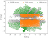 |
Fig. 1 Spatial distribution of our entire dataset. The gray points represent RR Lyrae stars identified by the OGLE survey and in a study by Dékány & Grebel (2020). Green points represent OGLE-identified RR Lyrae stars with VHS photometry. The orange points mark RR Lyrae stars classified by OGLE with the VVV mean intensity magnitudes from Molnar et al. (2022). |
2.1 OGLE-IV photometry
The fourth data release of OGLE (Soszyński et al. 2014, 2019) presents abundant photometry (with some stars having more than 15 000 observations) in V and I-passbands for more than 60 000 reliably classified RR Lyrae stars (68 127, in total used in this study). They provide the basic information on the variability, including mean apparent magnitudes in the I band, ephemerides (pulsation period P, time of maximum brightness M0), the amplitude of light changes (AmpI ) and some of the Fourier coefficients derived from the photometric light curves (R21, R31, φ21, φ31)2. The Fourier coefficients and pulsation periods can be used to estimate the photometric metallicities of individual RR Lyrae stars (e.g., Jurcsik & Kovacs 1996; Smolec 2005; Dékány et al. 2021; Mullen et al. 2022) and consequently absolute magnitudes.
While the OGLE survey provides extensive data, it does not include uncertainties for these values, except for pulsation periods. Consequently, to accurately estimate photometric metal- licities (using relations from Dékány et al. 2021) and absolute magnitudes, we recalculated the Fourier coefficients to obtain amplitudes A1 and A2 and phase differences φ31 and their uncertainties.
We decided to derive the mean intensity I-band magnitudes and Fourier coefficients based on an approach described in Petersen (1986). We optimized the following Fourier light curve decomposition:
 (1)
(1)
In Eq. (1), mI represents the mean intensity magnitudes, Ak and φk stand for amplitudes and phases. The n denotes the degree of the fit which we adapted for each light curve. We use the same approach as in Prudil et al. (2019a), with the minor modification that we enforced the fourth degree (n = 4) as a minimum (to obtain Fourier coefficients and their covariances for φ31 ). Due to the sparsity of the data, this condition was not applied to the V band. The ϑ represents the phase function defined as:
 (2)
(2)
where HJD is the heliocentric Julian date of the observation and M0 stands for the time of brightness maximum. The calculated Fourier coefficients and their uncertainties subsequently were used in the estimate of the photometric metallicities ([Fe/H]phot) using procedures described in Dékány et al. (2021)3. Based on the Fourier decomposition, we also obtained uncertainties on the mean intensity magnitudes,  , which we subsequently used in distance determination.
Furthermore, we also performed Fourier light curve decomposition on the less abundant data for the V band and obtained mean intensity magnitudes, mV with their associated uncertainties. The newly derived mV and mI and their associated uncertainties do not significantly differ from those provided by OGLE. Mean intensity magnitudes from multiple passbands for RR Lyrae stars can serve as a reddening indicator and thus improve distance estimations (e.g., Kunder et al. 2010; Haschke et al. 2011). Finally, we emphasize that OGLE-IV served as the main source of RR Lyrae identification in this work.
2.2 Gaia photometry
To obtain additional colors for distance estimation, we crossmatched our OGLE-identified single mode RR Lyrae stars (RRab and RRc) with the RR Lyrae variables identified in the third data release of the Gaia catalog (Gaia DR3, Clementini et al. 2023). Thus, we obtained source_id’s together with photometric (mostly between 25 to 45 observations in G band) and astrometric data for most of our RR Lyrae dataset (approximately 80%). This catalog also contains information on pulsation properties of identified RR Lyrae pulsators, but only the peak-to-peak magnitude in the G band is used in our analysis (see Table 1). We decided to keep OGLE pulsation properties as they are derived from a larger number of observations compared to Gaia.
For the remaining RR Lyrae variables identified by OGLE without a Gaia RR Lyrae counterpart (≈20%), we cross-matched the gaia_source dataset (Gaia Collaboration 2023) to obtain their associated mean flux magnitudes  , proper motions
  , and their associated uncertainties and correlations (in case of proper motions). We note that the gaia_source catalog does not provide an error on the mean magnitudes due to asymmetric error distribution in magnitude space, and only uncertainties on flux are provided. We converted their fluxes to magnitude space since we do not use the unidentified RR Lyrae stars in the Gaia catalog in the reddening estimation. We assigned them an uncertainty based on an error on the flux and variation in the zero-point4. In addition to photometric and astrometric properties, we also obtained some of the Gaia flags on the quality of photometry and astrometry, namely re-normalized unit weight error (RUWE5) and ipd_frac_multi_peak that refers to the detection of a double peak in image processing of a given object, possibly identifying sources of binarity or blending (Gaia Collaboration 2016b, 2023).
2.3 VVV photometry
We also collected IR photometry for bulge RR Lyrae stars from the VVV survey. VVV provides observations in the near-IR passbands (Z, Y, J, H, and Ks), where the most numerous are observations in the Ks band. VVV provides aperture photometry with five different apertures for each object (with, on average, 172 observations in Ks band). Therefore, it is up to the user to select an appropriate aperture. We collected individual observations provided in the photometric catalogs by the Cambridge Astronomy Survey Unit (CASU). As is shown by Hajdu et al. (2020), the VVV survey exhibits some issues with photometric zero-point calibration. Thus, before we proceeded with our analysis, we recalibrated the obtained Ks and J-band photometry using a procedure described in Hajdu et al. (2020) and implemented in the correct_vvv_zp code6.
To select the appropriate aperture, we proceeded as follows: we performed Fourier decomposition of the Ks -band observations using ephemerides and variability identification from the OGLE survey and measured the signal-to-noise ratio (SNR) as a cost function and estimated mean intensity magnitudes for individual apertures (see Dékány et al. 2021, for details). We defined the SNR using the following equation:
 (3)
(3)
where  represents total amplitude (peak-to-peak, between 0.1 to 0.5 mag) of the light curve, N_data is the number of observations, and RMSE represents the root-mean-square error. The appropriate aperture and subsequent mean intensity magnitudes were selected based on the maximum SNR value for a given RR Lyrae light curve. Using this approach, we obtained mean intensity magnitudes and their uncertainties
  for individual RR Lyrae variables observed by the VVV survey.
In addition to VVV Ks , we also obtained VVV mean intensity magnitudes for the J band. For individual RR Lyrae pul- sators, we used the same apertures as for the Ks-passband. We utilized the pyfiner7 (Hajdu et al. 2018) routine to estimate the corrected weighted mean J-band magnitudes.
To increase the number of RR Lyrae stars toward the Galactic bulge and to cover lower Galactic latitudes, we included in our catalog RR Lyrae stars identified by Dékány & Grebel (2020), in addition to the OGLE RR Lyrae dataset. The Dékány & Grebel (2020) dataset provides photometry in J, H, and Ks-passbands, and to estimate intensity mean magnitudes, we proceeded in the same way as in the case of the VVV photometry. Therefore, we obtained an additional ∼4000 fundamental-mode RR Lyrae stars with mean intensity magnitudes in J, H, and Ks -passbands, and pulsation properties (pulsation period and amplitude in Ks band). The newly acquired dataset was cross-matched with the Gaia catalog in the same way as is described in Sect. 2.2. Lastly, using the rrl_feh_nn8 (Dékány & Grebel 2022) module, we obtained photometric metallicities that were subsequently used for estimating the absolute magnitudes of individual RR Lyrae stars. Here we note that rrl_feh_nn is calibrated using essentially the same dataset as for relations used for I -band data from OGLE (Dékány et al. 2021).
Despite our best efforts to minimize possible blends by selecting a suitable aperture for a given RR Lyrae star in the VVV footprint, there was still a possibility of contamination by a nearby star. We compared our mean intensity magnitudes with a recent study by Molnar et al. (2022), which utilized VVV point spread function (PSF) photometry to search for variable stars toward the Galactic bulge. PSF photometry reaches a deeper limiting magnitude as well as improves the number of sources detected, which is helpful in crowded regions like the bulge (Surot et al. 2019). The bulge RR Lyrae stars have K ∼ 15 mag at the highly reddened low-latitude regions, which is still ∼3 magnitudes brighter compared to where PSF photometry has the most effect and where differences between PSF and aperture photometry are seen (e.g., Zhang & Kainulainen 2019). We matched our VVV dataset together with Molnar et al. (2022, comparison of ∼32 000 RR Lyrae single-mode pulsators) using Gaia source_id, and looked for differences between our mean intensity magnitudes and those determined in Molnar et al. (2022).
The comparison is depicted in Fig. 2, in which approximately 4% of matched pulsators exhibit systematically brighter apparent mean intensity magnitudes in our analysis. We separated this discrepant sub-population by using the absolute difference between both mean intensity magnitudes, where stars with values above 0.3 were marked with red points in Fig. 2. Selected variables based on the absolute difference also exhibit very low amplitudes, hinting toward blending with a nearby star that contributes its light to the selected aperture. We tried to mitigate the discrepancy by using a smaller aperture, but that only solved the problem in approximately one-third of the discrepant cases.
We noticed that the number of discrepant cases could be reduced by more than half if we remove stars with RUWE > 1.4 or with ipd_frac_multi_peak > 4. Therefore, we implemented both aforementioned criteria (see Eq. (4)) to clean our dataset of these problematic cases. In addition, the remaining stars that pass the two conditions but still deviate from Molnar et al. (2022, 41 310 and 39 517 stars with Ks and J band data, respectively) photometry have, on average, uncertainties on mean intensity magnitudes six times higher than are average uncertainties for a sample of RR Lyrae variable with difference below 0.3 mag. Despite that, we decided to use mean intensity magnitudes for J, Ks from Molnar et al. (2022) for stars matched with our dataset. We used only stars where pulsation periods matched those in our sample (∆P < 0.0001 day). We used the VVV aperture photometry described in the previous subsection (data from Dékány & Grebel 2020) for the remaining variables. Lastly, for stars from the Molnar et al. (2022) catalog, we used estimated photometric [Fe/H]phot from OGLE and VVV photometry described in Sects. 2.1 and 2.3.
Considering the significance and impact of blending in the direction of the Galactic bulge, we chose to apply the following criteria to our dataset for all subsequent analyses in this paper (unless otherwise specified):
 (4)
(4)
RR Lyrae variables that did not meet these conditions or that lacked the specified Gaia flags have been excluded from any analysis presented henceforth.
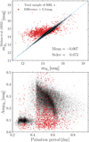 |
Fig. 2 Comparison of matched RR Lyrae stars in mean intensity magnitude space (top panel) and period-amplitude plane (bottom panel). The gray dots in both panels represent the total cross-matched sample (between our aperture VVV data and sample provided in Molnar et al. 2022), and red points stand for stars where the absolute difference between both mean intensity magnitudes exceeded 0.3 mag. To assess both photometric sources, we listed the mean and standard deviation between both samples (with discrepant RR Lyrae stars removed). The blue line in the top panel represents the identity line. |
2.4 The VISTA Hemisphere Survey
Lastly, to utilize the available data completely in order to counter the severe reddening, we explored matches (based on equatorial coordinates) between our RR Lyrae dataset and the VHS survey. The aim of the VHS is to map out the whole southern celestial hemisphere (excluding areas covered by other VISTA surveys) using the near-IR passbands (approximately 20 000 deg2). Contrary to the VVV survey, the VHS survey contributes single-exposure photometry in J, H, and Ks , complete with the corresponding modified Julian dates (subsequently converted to the HJD). Due to the longer exposure in Ks band, the VHS survey is approximately two magnitudes deeper (5σ at ≈20 mag) than the VVV survey (5σ at ≈ 18 mag). The difference in coverage between VVV and VHS surveys is displayed in Fig. 1.
We utilized publicly available data from the fifth data release of the VHS survey9. The DR5 contains only aperture photometry, which, as was shown in the previous Sect. 2.3, possesses a potential for blending of sources toward the Galactic bulge. To minimize this problem, we vetted our data in the following way. We required that none of our matched sources had a companion within 2 arcsec (due to the selected aperture) and that they fulfilled the criteria in Eq. (4).
These conditions reduced our matched catalog (over 25 000 objects) to approximately 11 000 stars with single epoch J, H, and Ks photometry. Due to the pulsation nature of our objects, to determine precise distances, we needed to estimate mean intensity magnitudes for our VHS dataset that sample our targets at random phases with a single exposure. We used the procedure described in Braga et al. (2018, 2019), which utilizes photometric templates and amplitude scaling relations to estimate mean intensity magnitudes for matched stars. The ephemerides necessary for this calculation were taken from data provided by the OGLE survey. Since only single exposures were provided for matched RR Lyrae stars, the uncertainties on mean intensity magnitudes were approximately a factor of ten larger in comparison with VVV mean intensity magnitudes. This translated into an increased average error in the distance by approximately 200 pc than for stars with VVV data.
3 Distances to individual RR Lyrae stars
In the following section, we estimate distances to individual RR Lyrae pulsators toward the Galactic bulge in our dataset. The severe reddening hampers the effort to calculate distances at the RR Lyrae population in the Galactic bulge. Fortunately, the near-IR photometry of our dataset and intrinsic properties of RR Lyrae variables (such as the period-absolute magnitude- metallicity relation, PMZ) can help counter the extinction. RR Lyrae stars are efficient for tracing reddening, enabling the creation of detailed extinction maps, provided there is adequate quantity and spatial distribution of these stars (see, e.g., Kunder et al. 2010; Haschke et al. 2011; Prudil et al. 2019a).
Previous studies of the RR Lyrae population toward the Galactic bulge used mainly PMZ relations from V and I- passbands (Pietrukowicz et al. 2015; Kunder et al. 2016, 2020; Du et al. 2020) combined with reddening laws and maps based on VVV photometry (Gonzalez et al. 2012; Nataf et al. 2013) to estimate distances. In this study, we followed an approach used in one of our previous works in which we used RR Lyrae stars themselves to trace extinction (Prudil et al. 2019a), particularly the reddening vector. The baseline for estimating reddening toward the Galactic bulge using RR Lyrae stars are reliable PMZ relations for available photometry (GBP, V, I, J, and Ks-passbands in our case). Therefore, we utilized recalibrated PMZ relations for our passbands from our previous work (Prudil et al. 2024a) and estimated absolute magnitudes and their uncertainties for all RR Lyrae stars in our sample.
To estimate the reddening vector, we used all single-mode RR Lyrae stars that have GBP, V, I, J, and Ks mean intensity magnitudes (at least two out of five) together with determined [Fe/H]phot based on their I and Ks -band photometric properties. We note that stars with VHS J and Ks magnitudes did not enter into the reddening law estimation for J – Ks and I – Ks colors. This was done due to the possibility of blending, which would severely affect available aperture photometry. It is important to emphasize that values for [Fe/H] used in the calibration of PMZ relations (Prudil et al. 2024a) were on the same metallicity scale as the [Fe/H]phot derived for our bulge sample. Therefore, no further conversion was necessary, and we could use metallicities directly estimated from photometry.
Unfortunately, not all RR Lyrae stars in our dataset have Ks mean intensity magnitudes. Thus, we also created reddening maps using GBP, V, and I passbands to fully utilize the available data, and provide up to four estimates of the color excess E (J − Ks), E (I − Ks), E (V − I), and E (GBP − I). Further, we note that for estimating the reddening vector for the color excess E (GBP − I), we used only RR Lyrae stars identified as variables by Gaia (Clementini et al. 2023).
Pulsation periods, together with [Fe/H]phot, allowed us to estimate absolute magnitudes  (using relations from Prudil et al. 2024a, see their Eqs. (16), (18), (19), (22), and (23)), which in turn we used to estimate the color excesses E (J − Ks), E (I − Ks), E (V − I), and E (GBP − I) described by the following equations:
 (5)
(5)
 (6)
(6)
 (7)
(7)
 (8)
(8)
To determine the distances to individual RR Lyrae stars, we assumed that reddening is uncorrelated with the distance modulus; for example,  . E (J − Ks), where the index 0 denotes dereddened quantities and
  represents the slopes of the reddening law. In Fig. 3, we present the spatial distribution of four derived color excess maps. These maps focus solely on the central parts of our dataset, closely aligning with the VVV footprint. This approach was specifically chosen to emphasize the central regions, where we have estimated the reddening laws and conducted the majority of our spatial and kinematic analyses.
The color excess and distance modulus (e.g.,  and mI − MI) then follow a nearly linear dependence, where the
  , and
, and  are the slopes of the reddening laws:
 (9)
(9)
 (10)
(10)
 (11)
(11)
 (12)
(12)
where  and AI are extinction values in respective bands toward a given RR Lyrae star. This assumption is discussed further below and consistently used in Figs. D.1, D.2, D.3, and D.4. The
  were then estimated through a linear fit between the color excess and distance modulus. In the first step, we needed to define bulge RR Lyrae stars because our RR Lyrae dataset covers the Sagittarius dwarf galaxy (Ibata et al. 1994), and the Sagittarius stream behind the Galactic bulge (see, e.g., Hamanowicz et al. 2016). RR Lyrae variables in the Sagittarius dwarf galaxy are further away and will be more reddened than stars in the bulge (see, e.g., Kunder & Chaboyer 2009). We used two linear relations to separate the Galactic bulge RR Lyrae stars from the foreground and background RR Lyrae population (similar to the selection in Pietrukowicz et al. 2015). The linear relations (in mean intensity magnitude and color space, see Table 2) had the following form:
 (13)
(13)
 (14)
(14)
We also included a cap for maximum mean intensity magnitude for individual reddening vector estimation to ensure the high completeness of our analyzed sample (marked with the horizontal red line in Figs. D.1, D.2, D.3, and D.4). In addition, to emphasize the point on blending (see Sect. 2.3), we again used criteria in Eq. (4). The values for alow , aupp , blow , and bupp are listed for individual color-magnitude combinations in Table 2. In the second step, we binned the color excesses over which we wanted to estimate reddening laws. We used a moving weighted average with a window size equal to 750 and a step size equal to 500 (stars) for all four passband combinations. We estimated the weighted average and the error on the mean of the respective distance modulus for each binned color excess region.
The results of linear fits, including their uncertainties and correlations between slope and intercept, and selection criteria are depicted in Appendix D (see Figs. D.1, D.2, D.3, and D.4). From the intercepts of our linear fits, we can approximately estimate the distance to the Galactic center. We note that in our method, we assume no physical correlation between distance and reddening (similarly to the approach by Alonso-García et al. 2017, using the RCs). This condition is not strictly met here, but since the majority of our targets are located away from the Galactic plane, where most of the dust resides, we consider a typical Bulge RR Lyrae to be behind the vast majority of the dust.
To estimate the distance to the Galactic center using our derived distances, we need to apply two geometrical corrections: (i) projecting onto the Galactic plane via cos b and (ii) correcting for the cone effect by scaling the distance distribution by a d−2 factor. Once we applied these geometric corrections, we focused on the region where our dataset has the highest completeness (within b = (−2, −6) deg and |ℓ| < 5 deg). We then estimated the distance to the Galactic center by fitting the cone-effect corrected kernel density estimate (KDE) with a Gaussian function:  = 8217 ± 1(stat) ± 528(sys) pc,
  = 8230 ± 1(stat) ± 379(sys)pc,
  = 8058 ± 1(stat) ± 974(sys) pc,
  = 7759 ± 4(stat) ± 861(sys) pc. The statistical and systematic uncertainties of individual distances to the Galactic center were estimated based on the uncertainties calculated for each distance in this section. The overall statistical and systematic uncertainties are the average values of these individual uncertainties. The statistical uncertainty is additionally scaled by the square root of the number of RR Lyrae stars used in the distance estimation. The estimated values are well within the accepted distance measurements for the Galactic center (GRAVITY Collaboration 2021; Leung et al. 2023). The coneeffect correction is depicted in Fig. 4 for
  .
.
Derived mean reddening laws based on single-mode RR Lyrae stars toward the Galactic bulge are listed in Table 3. The reddening law derived for  is a bit higher but still consistent within 1.5σ with those estimated in previous studies, such as
  = 0.428 ± 0.04 and
  = 0.443 ± 0.036 for Alonso-García et al. (2017) and Wang & Chen (2019), respectively. On the other hand,
  agrees well with the reddening law estimated by Nishiyama et al. (2006) equal to
  = 0.494 ± 0.006. Our estimate for
  is slightly smaller than the estimates of Dékány et al. (2013,
  = 0.164) and Nataf et al. (2013,
  = 0.160) and to a degree higher than the estimate from Prudil et al. (2019a,
  = 0.140). In addition, our RVI value matches with the estimate by Nataf et al. (2013, RVI = 1.215). Newly defined reddening laws subsequently served in estimating distances toward bulge RR Lyrae stars through the distance modulus:
 (15)
(15)
 (16)
(16)
 (17)
(17)
 (18)
(18)
The uncertainties on individual distances were calculated by including all sources of errors (from the mean intensity and absolute magnitudes, reddening law, and color excess). We also divided our sources of uncertainty into statistical10 and systematical categories11 where systematic uncertainties dominate the error budget (≈95 of the total uncertainty on distance).
In our approach, uncertainties on distances purely from VVV photometry uncertainties constitute approximately 6% of the total distance. When we combine VVV Ks band and OGLE I band, we reach an uncertainty on the distance as low as 4%. The increase in precision is due to removing the need to use the J band, which has a larger scatter in the PMZ relation, and due to fewer photometric epochs in VVV. Distance uncertainties using purely visual passbands contribute to an uncertainty of around 10–11%. The derived uncertainties on distances are slightly higher when compared with previous studies (particularly with the precision of ten and 3% for optical and IR data, respectively, Neeley et al. 2017). The full table with derived photometric metallicities, absolute magnitudes, color excesses, and distances for all sample RR Lyrae stars is included in Appendix C.1 and as a supplementary material for this paper. The verification of our distances is included in Appendix A.
Lastly, we emphasize that using a single reddening law for the entire Galactic bulge region is a suboptimal solution. Variations from the commonly assumed Cardelli et al. (1989) extinction law have been reported at low Galactic latitudes (Nishiyama et al. 2005, 2006, 2009). The decision to use a single reddening law was imposed by the low stellar density of RR Lyrae variables in this region, which prohibits the estimation of the reddening law in binned coordinate space.
Linear relations and conditions used to remove foreground and background RR Lyrae stars from our dataset for reddening vector estimation.
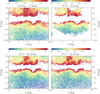 |
Fig. 3 Spatial distribution of color excesses estimated in this study, E (GBP − I), E (V − I), E (I − Ks), and E (J − Ks). Each point represents a given single-mode RR Lyrae star color-coded based on its associated reddening. Note the different color scales in each panel. |
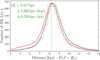 |
Fig. 4 Distance distribution of |

Estimated reddening laws in this study and the number of RR Lyrae stars (N✶) used for each reddening law.
4 Comparison of reddening maps
4.1 Comparison of derived reddening maps in this study
In the following analysis, we compare the estimated extinction toward RR Lyrae stars derived from our reddening maps. Our focus is on comparing the predicted AI values, which are based on different color excesses derived using both visual and IR passbands. This approach is motivated by the studies of Dékány et al. (2013) and Pietrukowicz et al. (2015), which employed different passbands for distance estimation and reported somewhat contradictory results.
To achieve this, we need to transform reddening laws for E (J − Ks) and E (I − Ks) to obtain AI. For these transformations, we utilized the results for  from Sect. 3. For E (I − Ks), we calculated the extinction in the I band as follows:
 (19)
(19)
 (20)
(20)
 (21)
(21)
 (22)
(22)
 (23)
(23)
For E (J − Ks), we used the following approach:
 (24)
(24)
 (25)
(25)
 (26)
(26)
 (27)
(27)
Using the derived Eqs. (23) and (27), we calculated the extinction through E (I − Ks) and E (J − Ks) for the I band.
In Fig. 5, we present the binned spatial maps (with a bin step equal to 0.5 deg in both directions) showing the difference in AI (denoted as ∆AI) and its variation with respect to Galactic longitude. Significant variation in AI as a function of both Galactic longitude and latitude is evident. Focusing initially on the Galactic latitude variation, the middle and right panels indicate that closer to the Galactic plane, E ( J – Ks) predicts smaller AI values than E (V – I) and E (I – Ks). In contrast, for AI based on E (GBP – I), the trend reverses near the Galactic plane, with E ( J – Ks) predicting higher AI values. These fluctuations underscore the challenges in estimating reddening near the Galactic plane, especially with broad visual passbands.
To investigate the Galactic longitude variation, we examined the region b = (−6, −2) degrees, previously studied for indications of the bar traced by RR Lyrae stars (Pietrukowicz et al. 2015). We observe a notable divergence in AI in Galactic longitude, which is especially evident in the insets of Fig. 5. A distinct gradient is observed, particularly in the visual passbands (left and middle panels). Notably, at positive l, there is a bump in ∆AI with an amplitude of approximately 0.25 mag for both visual reddenings. For E (V – I), a decrease in ∆AI at negative ℓ is also noticeable. Assuming the AI based on E ( J – Ks) is accurate, these discrepancies could lead to distance underestimation at positive ℓ and overestimation at negative ℓ. Such AI variations could result in a distance difference of about 1 kpc for Galactic bulge stars. Referring to Fig. 3 in Gonzalez et al. (2011), the distance difference between ℓ = (−5, 5) degrees is around 1 kpc. Therefore, it is crucial to acknowledge that a shift of several hundred parsecs, observed in visual passbands, could mimic the appearance of the bar. In the right panel, the bump is less pronounced, with an amplitude less than half that for visual passbands. The ∆AI variation is not as significant as in the visual passbands, highlighting the importance of using IR passbands for estimating extinction and distances toward the Galactic bulge.
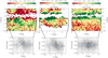 |
Fig. 5 Binned spatial distribution (step equal to 0.5 deg) of differences in estimated extinction ∆AI. Each panel depicts the differences between the extinction (AI) estimated from purely optical or near IR-optical color excesses (E (GBP – I), E (V – I) and E (I – Ks)), and the extinction estimated from the E (J – Ks) color excess. The insets focus on an area below the Galactic plane where we binned (blue circles, seventeen steps between −9.5 to 9.5 deg) the ∆AI as a function of ℓ with gray dots representing individual RR Lyrae stars. |
4.2 Comparison of derived reddening maps with literature
Following up on the previous subsection, we replaced the E ( J – Ks) values derived in this study with data from the literature, specifically the reddening map from Surot et al. (2020)12 and the Gonzalez et al. (2012, using the Bulge Extinction and Metallicity Calculator, BEAM213) studies. We matched our dataset with the reddening maps using equatorial and Galactic coordinates. Both cited studies utilized RC stars identified in the VVV survey to assess reddening toward the Galactic bulge. We performed the same comparison as in Fig. 5, employing Eq. (27). We selected these two studies specifically because they provide direct E ( J – Ks) measurements. Both studies are based on VVV data, the main difference is in the use of aperture photometry (Gonzalez et al. 2012) vs PSF photometry for the more recent study by (Surot et al. 2020) and the bin sizes of provided maps.
The comparison based on the Surot et al. (2020) reddening map is depicted in Fig. D.5, while the comparison based on the Gonzalez et al. (2012) reddening map is shown in Fig. D.6 and included in the appendix. Both reddening maps present a picture similar to the analysis in Fig. 5. For both visual-based color excesses, we observe mostly larger ∆AI at positive l and lower ∆AI at negative ℓ . The AI gradient in these reddening maps is shallower than ours but still shows a total amplitude of about 0.15 mag, equivalent to approximately 600 pc at the distance to the Galactic bulge. Assuming the extinction in the I band estimated using E ( J – Ks) is correct, this could result in a bar-like tilt (of a smaller angle than found using RC stars by Wegg & Gerhard 2013) in the visual distances for RR Lyrae stars.
In the right panel of Figs. D.5 and D.6, we note that the extinction AI estimated using E (I – Ks) is underestimated by approximately 0.05 mag and 0.08 mag, based on the reddening maps from Surot et al. (2020) and Gonzalez et al. (2012), respectively. This results in a shift in distances of about 200 pc and 300 pc at the distance of the Galactic bulge, respectively, and remains more or less consistent across the majority of Galactic longitudes. The reason for this shift for both references is probably the absolute magnitude calibration of the photometric VVV system. This calibration is based on the catalog that is a result of crosscorrelation between the Two-Micron Sky Survey (2MASS, Cutri et al. 2003; Skrutskie et al. 2006) and VVV survey performed by the Cambridge AstronomySurvey Unit (CASU14).
4.3 Using reddening E(V – I) from the literature
The previous two subsections explored the variation between reddening maps derived in this study and those available in the literature for the Galactic bulge. We used E (J – Ks) as a reference for our comparisons. In the following analysis, we use the E (V – I) value from Nataf et al. (2013)15 to estimate AI and compare the obtained values with those calculated from our E (J – Ks), as well as E (J – Ks) values from Gonzalez et al. (2012) and Surot et al. (2020). We again utilize Eq. (27) to derive AI.
Figure D.7 presents the comparison. Observing the AI variation with respect to Galactic longitude, we note a consistent gradient along ℓ, as was seen in the previous two comparisons. There is an overestimation of AI from visual color excess at positive Galactic longitudes and a decrease in AI toward negative Galactic longitudes. For literature-based reddening maps, we obtained amplitude variations around 0.13 mag (0.5 kpc at the distance to the Galactic bulge), while for AI estimates based on our E ( J – Ks), we found an amplitude of 0.28 mag (approximately 1.1 kpc difference in distance).
The consistently observed gradient for 5 > ℓ > −5 further supports the conclusions from this section. Assuming the obtained color excess E (J – Ks) in this study and in studies focused on the Galactic bulge is correct, we conclude that the usage of visual passbands for RR Lyrae stars toward the Galactic bulge, as a means to obtain reddening, leads to potential spurious distance gradients along Galactic longitude. These gradients, despite uncertain total amplitude, result in a shift in distance ranging from 0.5 to 1.0 kpc between positive and negative longitudes. Depending on the amplitude, such a shift in distance can mimic the tilt of the bar as observed in RC stars (assuming a 1 kpc difference between the RCs at ℓ = −5 and ℓ = 5 deg, Gonzalez et al. 2012; Wegg & Gerhard 2013). We observe a shift between extinction estimated in this study compared to literature values; this shift appears systematic and does not exceed 300 pc (see the previous Sect. 4.2 on the probable cause of this shift). Therefore, it is fully covered by the error budget, contributing only to the average distance shift to the Galactic bulge.
5 Galactic bulge in 3D
The following section is inspired by and provides a comparison with earlier studies that focused on the spatial characteristics of the bulge RR Lyrae population, primarily those by Dékány et al. (2013) and Pietrukowicz et al. (2015). In what follows, we examine the spatial distribution of RR Lyrae variables toward the Galactic bulge, represented in heliocentric Cartesian coordinates (X, Y, and Z). To assess the spatial properties of the Galactic bulge, we aim to test the presence and orientation of the bar. Our methodology for estimating the angle of the bar was inspired by the approach outlined in Pietrukowicz et al. (2015). In our approach, the distance distribution is described by a Gaussian mixture model (GMM, from scikit-learn Python library Pedregosa et al. 2011). Based on testing the GMM using the Bayesian information criterion (BIC) and the Akaike information criterion (AIC), we utilized three GMM components in all cases. The AIC and BIC did not show significant changes with an increased number of GMM components. Using the GMM, we estimated density levels, specifically using the half-maximum of the distribution as a reference. Similar to Pietrukowicz et al. (2015), we projected our distances onto the Galactic plane using cos b. We divided our data into eleven bins based on Galactic longitude, ranging from −5 to 5 degrees. For each bin, comprising measured distances and their uncertainties, we estimated the half maxima of the distribution using the GMM. To account for uncertainties in distance, we employed a Monte Carlo simulation (with 1000 iterations) to vary distances within their error margins (assuming a normal distribution). The individual halfmaxima bins and their uncertainties were determined using the median and absolute median deviation.
The obtained half-maxima distances (and their uncertainties), along with median Galactic longitudes and latitudes, were used to estimate X and Y coordinates. Errors on X and Y were derived from the uncertainties in the distances. For distances obtained using methods and reddening maps from the literature, we used a single value for distance uncertainty, σd, set at 600 pc. To determine the inclination angle of the bar, ι, we fitted the binned Cartesian coordinates to an ellipse (as per the approach used by Pietrukowicz et al. 2015).
An ellipse is a particular form of conic section that can be defined by a quadratic polynomial equation:
 (28)
(28)
where a, b, c, d, e, and f are the Cartesian conic coefficients of the fit. This definition has a specific constraint on parameters a, b, and c; where b2 – 4ac < 0. Our method is somewhat similar to the fitting method described in Halir & Flusser (1998), which involves fitting an ellipse to given data points by minimizing the algebraic distance using a least squares approach (for Eq. (28)). It forms a model matrix from the data points, solves a generalized eigenvalue problem to enforce the ellipsespecific constraint, and extracts the ellipse parameters from the eigenvector corresponding to the smallest positive eigenvalue16. To incorporate uncertainties in the individual X bins, we conducted a Monte Carlo error analysis, varying X values within their uncertainties and recalculated ellipse parameters for each iteration. The inclination angle of the bar was then obtained using the following relation:
 (29)
(29)
Besides the ι between the semimajor axis and the x-axis, we also obtained values for the semimajor (a) and semiminor (b) axes17, which we used to estimate the b/a ratio. We report both the angle and axis ratio as the average and standard deviation of the resulting parameter distribution. Figure 6 illustrates an example of our analysis, showcasing the measurement of the bar inclination angle (for conditions on distance, please refer to Sect. 5.2 and conditions in Eqs. (30), (31), and (32)). In the following sections, we present the optimal values of ι and σι as measurements of the bar angle relative to the line of sight for our dataset. Lastly, we report the quality of the ellipse fit for each angle measurement. Although the ellipse may not always be the optimal model for the underlying distance distribution, we have used it here to facilitate a comparison with the work of Pietrukowicz et al. (2015) and to obtain an approximate estimate of the bar parameters. Each following spatial plot for which we measured the bar angle is also accompanied by contours (marked with green lines) based on the KDE. The contour levels were selected to avoid our spatial distribution’s center and edges to evade distortion.
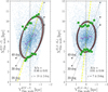 |
Fig. 6 Example of ellipse fitting (red line) to the spatial distribution of RR Lyrae stars (blue points). We used distances from this study estimated based on E (V – I) (left panel) and E (J – Ks) (right panel) color excesses. The green squares (used to derive ellipse parameters) and purple triangles represent the half-maximum and maximum of the GMM in a given bin (eleven bins between ℓ ≥ −5 and ℓ ≤ 5 deg). The different bar angles are outlined with dashed and dotted solid black lines. The dashed yellow and dotted black lines mark the measured and zero angles, respectively. The fit quality expressed using χ2 are 0.36, and 0.40 for left and right panels, respectively. |
5.1 3D spatial distribution
To analyze the spatial distribution, we used different approaches to estimate the distance (combination of visual and near-IR passbands), particularly the distances estimated in the previous section, Sect. 3. Moreover, we looked at the distance distributions derived in previous studies, particularly the seminal work of Pietrukowicz et al. (2015) and Molnar et al. (2022). The former work utilizes PMZ relations from Catelan et al. (2004) together with reddening maps by Gonzalez et al. (2012) and reddening law from Nataf et al. (2013). The latter study used IR passbands in combination with Wesenheit magnitudes (Madore 1982), period-metallicity-Wesenheit magnitude relations from Cusano et al. (2021), and  from Alonso-García et al. (2017). We also applied the same criteria as in Pietrukowicz et al. (2015) to create a dataset with identical stars that differ in distance estimation method. Lastly, we calculated Cartesian coordinates for each set of distance estimates (X, Y, and Z centered on the Sun). Therefore, we compared the same stars with different distance estimates (in total, more than 16 000 RR Lyrae variables). To compare their distribution with the position of the bar, we used data provided by Gonzalez et al. (2011). We note that we shifted the bar distance to match our Pietrukowicz et al. (2015) and Molnar et al. (2022) distances. Lastly, in this case, we did not use Gaia flags to remove possible blended objects (conditions in Eq. (4)), since the aforementioned studies did not use these criteria either. On the other hand, when estimating the tilt of the bar, we focused on the area below the Galactic plane (−6 ≤ b ≤ −2), similar to the study by Pietrukowicz et al. (2015).
In Fig. 7, we present our spatial comparison. In the top three panels, we show the distance distribution in Cartesian coordinates derived in this study. For the distances derived based on E (J – Ks) and E (I – Ks), we see much smaller values for the bar angle. There is no significant tilt in the direction of the bar as observed by Gonzalez et al. (2011). Using the method described at the beginning of this section, we found the bar angle for distances estimated using E (J – Ks) and E (I – Ks); ι = 6 ± 2deg and ι = 6 ± 2 deg, respectively. For the distances estimated purely from visual passbands (E (V – I), top right plot), we see a tilt with the bar (ι = 17 ± 2 deg), and additional substructure, “spikes,” in the bulge spatial distribution. A similar structure is also visible in the bottom right panel, where we show the Cartesian spatial distribution based on distances derived in Pietrukowicz et al. (2015). This panel shows the tilt (ι = 16 ± 2 deg) that suggests the bar’s position. We also see a similar substructure variation as for the distances derived using E (V – I). The aforementioned spikes are also visible in the top panel of Fig. 1 in Du et al. (2020, see their Y vs. X plane). The origin of these spikes does not appear to be physical but perhaps associated with the reddening and reddening law itself. These spikes are most prominent in regions above the Galactic plane (b > 0 deg where the reddening is higher than below the plane).
The lower middle and bottom left panels of Fig. 7 show Cartesian coordinates for RR Lyrae variables with distances derived through the procedure described in Molnar et al. (2022). The lower middle panel shows the entire Molnar et al. dataset, and the bottom left plot shows only stars in common between Molnar et al. (2022) and Pietrukowicz et al. (2015). We do not find a strongly tilted bar in either of the two panels (lower middle and bottom left). The angles found are ι = −0.9 ± 0.3 deg and ι = 10 ± 3 deg, for the lower middle and bottom left panels, respectively. We see a rather smooth distribution, similar to our distances estimated based on E (J – Ks) andE (I – Ks), without any substructure seen in the distances derived through visual passbands.
To summarize, we spatially recovered the bar-like feature and its angle from the use of distances based on visual passbands. The measured angle agrees reasonably well with previous bar angle measurements using RC giants, ι = 20–30 degrees (see, e.g., Wegg & Gerhard 2013; Simion et al. 2017; Leung et al. 2023; Vislosky et al. 2024). When using distances obtained from near-IR data, we detect only a negligible tilt for a bar-like structure. The appearance of the bar in visual passbands is likely connected to the gradient in ∆AI observed for visual passbands in Sect. 4. In previous studies using optical photometry only, this gradient in AI is not correctly accounted for in distance determinations to RR Lyrae stars.
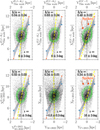 |
Fig. 7 Spatial distribution of RR Lyrae pulsators used for comparison in the Cartesian space. Individual subplots display different distance estimates based on near-IR (left column), a combination of near-IR and visual, and only visual reddening. The top panels show Cartesian coordinates derived based on distances estimated in this study. The bottom panels display the distances derived based on procedures from Pietrukowicz et al. (2015) (P+2015, bottom right panel) and Molnar et al. (2022) (M+2022, middle and bottom left panel). We also show two tentative bar angles with red triangles (20 degrees) and blue circles (30 degrees) and a shaded region marks the angles in between. Note that the Sun is at X = 0 and Y = 0 kpc. As is depicted in Fig. 6, the measured and zero angles are marked with dashed yellow and dotted black lines. Lastly, the χ2 of each fit from top left to bottom right are: 0.56, 0.57, 0.35, 0.51, 15, and 0.39. |
5.2 Visual versus infrared investigation of the discrepancy
In the previous subsection, we conducted a comparative analysis between the distance estimates for RR Lyrae stars toward the Galactic bulge found in the existing literature and our own estimates. We observed a notable discrepancy: distances derived primarily from IR passbands present a different perspective on the substructure of the bulge compared to those based on visual passbands (mirroring the divergence found in Dékány et al. 2013; Pietrukowicz et al. 2015). Our distance estimates using the E (V – I) color-excess reproduce very well the substructure traced by Pietrukowicz et al. (2015) even though Pietrukowicz et al. (2015) used different period-luminosity relations and their approach in the treatment of extinction also differed from ours. In this subsection we attempt to rectify this discrepancy by using alternative sources of reddening for visual passbands and examining the resulting spatial distribution.
We first used E (J – Ks) andE (I – Ks) to estimate the extinction in I band. Using the derived Eqs. (23) and (27), we can calculate the extinction through E (I – Ks) and E (J – Ks) for I band. In this comparison, we also used bulge extinction maps from Gonzalez et al. (2012) and Surot et al. (2020), which provide E (J – Ks) independent of our measurements, and through Eq. (27), we can transform them into AI . We also utilized RVI from a study by Nataf et al. (2013), which is based on OGLE passbands and RC stars. In the following comparison, we used Eq. (4), and we also imposed the following conditions on the dataset to focus on the Galactic center region with the highest completeness and purity of the OGLE RR Lyrae sample:
![Mathematical equation: $- 10 < \ell [{\rm{deg}}] < 10,$](/articles/aa/full_html/2025/03/aa50620-24/aa50620-24-eq78.png) (30)
(30)
 (31)
(31)
![Mathematical equation: ${\rm{and }}1.0 < d[{\rm{kpc}}] < 20.0.$](/articles/aa/full_html/2025/03/aa50620-24/aa50620-24-eq80.png) (32)
(32)
The newly calculated spatial distributions using various sources for reddening for estimation AI are depicted in Fig. 8. In this figure, we see a clear distinction between the spatial distribution estimated using our E (V – I) color-excess, and the ones with reddening estimated through near-IR passbands (E (I – Ks) and E (J – Ks)). The disparity is also quantified in the measured bar angle, where our distances based on visual passbands yield an apparent tilt angle of the bar around 18 ± 2 deg, while all other near-IR reddening estimates provide shallower and sometimes insignificant angles. In addition, using the varying reddening law from Nataf et al. (2013, RVI), we also observe a shallower angle for the bar. Based on this comparison, it appears that the reason behind the discrepancy in studies like Dékány et al. (2013) and Pietrukowicz et al. (2015) is the use of E (V – I) reddening and a single reddening law. Therefore, the observed gradient along the Galactic longitude in extinction difference, ∆AI, found in Sect. 4 for visual passbands appears to mimic the tilt of the bar but is an artifact of the dust properties.
To further explore the discrepancy between visual and near- IR sources of extinction, we compared two Galactic longitude bins where the difference between the bar inclination is the most significant among visual and near-IR-based color-excesses. In this comparison (depicted in Fig. 9), we did not use any reddening source from the literature and instead used only color-excess and reddening laws estimated in this work. We focused on the following two bins:
 (33)
(33)
 (34)
(34)
We compared the estimated AI based on E (V – I) and E (I – Ks) (solid blue and red lines in the bottom left histogram). We also included a comparison for AI estimated using E (I – Ks) and E (J – Ks) (dashed blue and red lines in the bottom left histogram) which served as a baseline for the comparison.
The assessment showed that the average difference between AI calculated using E (I – Ks) and E (J – Ks) in both bins is negligible (accounts to 0.02 mag which translates to approximately 80 pc at a distance to the Galactic bulge). On the other hand, the average difference in AI estimated from E (V – I) and E (I – Ks) is almost a factor of six larger (0.12 mag in ∆AI, in distance approximately 470 pc). This disparity only grows larger for more reddened stars and reaches above 1 kpc. This analysis is in agreement with the results presented in Sect. 4.1.
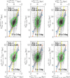 |
Fig. 8 Similar to Fig. 7, we depict spatial distribution bulge RR Lyrae variables using absolute and mean intensity magnitudes (in I band) together with different methods to account for extinction toward the Galactic bulge. The top three panels show spatial distributions derived using color excesses calculated in this work. The bottom two panels show the same spatial distributions but for distances estimated using literature reddening maps toward the Galactic bulge (from left to right, Nataf et al. 2013; Surot et al. 2020; Gonzalez et al. 2012). To measure individual bar angles we binned spatial dataset into eleven bins between ℓ ≥ −5 and ℓ ≤ 5 deg). As in Fig. 6 we depict measured and zero angles with dashed yellow and dotted black lines, respectively. The χ2 for each fit from top left to bottom right are 0.39, 3.4, 0.37, 1.6, 1.4, and 0.43. |
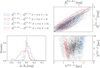 |
Fig. 9 Comparison of AI extinction estimates in two Galactic longitude bins. The red lines and points represent the bin at positive Galactic longitudes, while the blue points and lines represent stars at negative Galactic longitudes. The dashed lines in the histogram represent the difference in AI for near-IR-based color-excesses, while solid lines show the difference for mainly visual passband-based color-excesses. |
5.3 Spikes
To investigate the nature of the spikes and substructure variation, we explored the possibility of variation in the reddening law by selecting three regions in the Galactic bulge based on the Galactic longitude. There, we independently determined reddening laws for E (V – I) and for comparison also for E (J – Ks) in the same way as in Sect. 3 but with smaller bins (50) and step size (20). We note that we did not restrict our dataset in the Galactic latitude. The results of this analysis are listed in Table 4 and displayed in Fig. D.8. We found a significant variation in RVI based on Galactic longitude and also small changes in  . When we apply the modified RVI based on the star’s Galactic longitude, it leads to a small decrease in the substructure visible in Fig. 7 (see panel with modified distances in Appendix D.8). The spikes do not fully disappear since the variation in the reddening law is most likely on sub-degree levels, and we did not consider changes in reddening law in the Galactic latitude direction (Nataf et al. 2013; Schlafly et al. 2016). We also report a change in reddening law for
  albeit smaller than for RVI . Quantitatively speaking, the variation in RVI results in changes in distances on average of 0.6 kpc while for
  the changes are on average below 0.2 kpc.
To further explore the origin of these spikes, we compared for this dataset our reddening values for E(J – Ks) and E(V – I) with values estimated based on work by Pietrukowicz et al. (2015). In Fig. D.9, we displayed our comparison and noticed a clear linear trend with a minimum offset and scatter lower than our average uncertainty on E(J – Ks). We also displayed stars approximately associated with the two spikes shown in Fig. 7 (selected based on their X and Y coordinates, particularly in regions with X > 8.5 kpc). Variables in these spikes do not deviate from the overall trend in E(J – Ks) and E(V – I) reddening comparisons. Their reddening does not appear to be over or under-estimated. We emphasize that we are comparing E(J – Ks) derived here with E(J – Ks) from Gonzalez et al. (2012), and E(V – I) estimated in this work with E(V – I) calculated using the method outlined in Pietrukowicz et al. (2015). We do not compare the extinction derived from E(J – Ks) from E(V – I) as we did in Sect. 4.
Thus, the probable reason behind the spikes lies more on the visual side of the reddening and reddening law itself. This is supported by the spikes being more prominent in the spatial map derived using our estimated E(V – I) but not the spatial map derived by E(J – Ks). The visual passbands are more affected by extinction, and varying the reddening law in the Galactic latitude and longitude (as is seen, e.g., in Nishiyama et al. 2006; Nataf et al. 2013; Schlafly et al. 2016) could result in a suitable mix for artificial structures to appear in the spatial distribution. For example, in our work, we use a single universal reddening law for all variables in our dataset. This might work well for the near-IR data (smooth distribution in spatial properties, see top panels of Fig. 7), where the reddening variations are subtler, thus leading to a much lower impact on the results. On the other hand, such a universal “single reddening law” approach probably fails in the visual, where even if the reddening values agree with those determined by different methods (see Fig. D.9), the likely variation in the reddening law in the Galactic longitude and latitude in a reddening sensitive part of the spectrum creates artificial substructures. Lastly, the severity of the difference between reddening treatment for distances from purely J and Ks, and those derived only from V and I is that reddening is, on average, three times higher for the latter. This emphasizes the importance of proper extinction treatment toward the Galactic bulge, especially when using visual passbands where the variation in reddening law should be included. Lastly, the known issue of the VVV photometric calibration (see Hajdu et al. 2020) is most likely not responsible for these spikes since we also see them in our distance calibration for E (V − I) where we did not use VVV photometry.
Variation in the reddening law.
6 Metallicity and spatial distribution
We explored the differences in spatial properties of our RR Lyrae dataset by dividing it into two groups based on estimated photometric metallicity. We categorized the dataset into metal-poor ([Fe/H]phot < −1.0 dex) and metal-rich ([Fe/H]phot > −1.0 dex) RR Lyrae stars with distances estimated using near-IR (E(J − Ks)) passbands. The boundary between the metallicity bins was selected based on Fig. 12 and by the work of Crestani et al. (2021a) and Prudil et al. (2020), where we see that metalrich RR Lyrae stars with spectroscopic [Fe/H] > −1.0 dex have, in general, a very low [α/Fe] abundance, and thus the halo contamination in the metal-rich bin should be minimal.
6.1 Different approach in estimating bar angle
In this section, we implement a different approach to estimate the bar angle of the metal-rich RR Lyrae population due to their scarcity, and to trace the bar angle across different metallicity bins. Specifically, we used the inertia tensor (assuming all masses are equal to one) and its eigenvalues to estimate the bar angle and the axis b/a ratio. In this method, we calculated the cylindrical radius (Rcy1) using the Cartesian coordinates X and Y, and used only stars within a given limit,  .
.
To test this method, we first conducted a simple simulation in which we generated two sets of spatial (X, Y, and Z) distributions. The first set consisted of a uniform (unbarred) distribution across all three Cartesian coordinates:
 (35)
(35)
 (36)
(36)
 (37)
(37)
The second set followed an ellipsoidal distribution with the spatial properties of the Galactic bar (ι = 27 deg, b/a = 1.0/2.1, and c/a = 0.82/2.1, based on Wegg & Gerhard 2013). Both distributions were convolved with our estimated distance uncertainties (6% for E(J − Ks) distances) and restricted based on our “cone view” of the Galactic bulge (Fig. 6) to better simulate our observational dataset. The two distributions were then combined, keeping the size of the ellipsoidal population fixed while increasing the size of the axisymmetric population. We also varied the limiting  and examined how these changes affected the recovered bar angle and b/a axis ratio. For comparison, in addition to the cone view, we included the full simulated dataset, unconstrained by the cone.
In Fig. 10, we present our test results. From the unconstrained view, we observe that the true bar angle is never accurately estimated. Despite variations in the limiting  and the size of the axisymmetric population, the bar angle consistently fluctuates around 19 deg in nearly all cases. This effect is due to the convolution of the simulated distributions with our distance uncertainties, which cause the bar angle to appear smaller (Hey et al. 2023; Vislosky et al. 2024; Zoccali et al. 2024). The situation is similar for the cone view; the true bar angle is never fully recovered. Only for the smallest values of
  , and with minimal contamination from the axisymmetric population, does the measured bar angle reach 18–19 deg, constrained by the distance uncertainties. On the other hand, for the axis ratio, higher values of
  better capture the overall axis ratio, despite the presence of distance errors.
In the end, we decided to use  kpc for our observational dataset. This decision was driven by the test above and by the narrowness of our dataset in Y coordinate (Fig. 6). By including stars from larger cylindrical radii we would preferentially select variables in the foreground and background of the Galactic bulge while not increasing the amount of stars in the bar region.
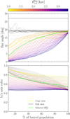 |
Fig. 10 Test of the inertia tensor method for estimating the bar angle (top panel) and the b/a axis ratio (bottom panel) for our simulated dataset. The solid black lines represent the simulated, unrestricted view of the Galactic bar for different values of |


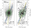 |
Fig. 11 Spatial distribution analysis for near-IR distances derived using E(J − Ks). The right and left panels show metal-poor ([Fe/H]phot < −1.0 dex) and metal-rich ([Fe/H]phot > −1.0 dex) RR Lyrae variables in our dataset (black dots). Two approximate bar angles (20 and 30 degrees) are shown with red triangles and blue circles, respectively with shading marking the angles in between. Similar to Fig. 6, we show measured and zero angles with dashed yellow and dotted black lines. Lastly, the quality of the ellipse fit for the left panel is χ2 = 0.45. |
6.2 Bar angle as a function of metallicity
We again applied conditions in Eq. (4) and selected stars within b = (−2, −6) and |ℓ| < 10 degrees. In Fig. 11 we display comparisons for both metal-rich and metal-poor samples. We see that the prominence of the bar angle changes differs for both metallicity groups. Specifically, the metal-poor population shows little to no indication of the bar, as is evidenced by the low bar angle (ι = 6 ± 2 deg). We note that the value of the bar angle in this case was derived using the ellipse fitting method (described in Sect. 5). We also used the inertia tensor approach to verify this value, obtaining ι = 9 ± 1 deg and b/a = 0.82 ± 0.01. Furthermore, we implemented a modified 2D version of the inertia tensor method described in Zemp et al. (2011); Pulsoni et al. (2020, see Sect. 4 of the latter). This method iteratively determines the bar angle and axis ratio. The initial selection of stars is adjusted iteratively to better match the ellipsoidal shape of the bar. After each iteration, the axis ratios and bar angle are updated based on the newly selected set of stars, according to the current estimate of the bar’s orientation and ellipticity. This process is repeated until a specified convergence criterion is met (in our case, when the change in the axis ratio between iterations is smaller than 1%). Using this approach, we obtained ι = 5 ± 1 deg and b/a = 0.58 ± 0.01, once again confirming the low bar angle for the metal-poor RR Lyrae population.
Conversely, the bar signature is clear in the metal-rich population, with a tilt of ι = 18 ± 5 deg18. We note that the derived bar angle is lower but within the errors in agreement with what is typically assumed for the Milky Way bar based on RC stars. This discrepancy may be attributed to the low number of RR Lyrae stars in our metal-rich bin (suggesting that the Galactic bulge does not contain many metal-rich RR Lyrae pulsators) or to kinematic fractionation. According to Debattista et al. (2017), kinematic fractionation occurs when initially co-spatial stellar populations with different in-plane random motions (radial velocity dispersions) separate during bar formation and evolution. Metal-poor populations, which are generally older and have higher radial velocity dispersions, tend to form a weaker bar and become vertically thicker, leading to a boxy bulge structure. On the other hand, metal-rich populations, with lower initial radial velocity dispersions, form a stronger bar and a more pronounced peanut-shaped bulge. This difference in bar strength and shape could potentially lead to a tilt between the metal-poor and metalrich populations. However, as is indicated by the simulations, this effect may not be universally applicable and could depend on specific initial conditions of the bulge and the evolutionary history of the bar (Debattista et al. 2017; Fragkoudi et al. 2017). Lastly, we note that the difference between the bar angles derived from metal-poor and metal-rich populations is on the margins of being statistically significant (pvalue = 0.03).
Furthermore, we explored the bar angle’s and axis ratio’s dependence on the metallicity of RR Lyrae stars. In this examination, we used solely the angle and axis ratio derived from the inertia tensor and its eigenvalues. We used a moving boxcar method to split our metallicity distribution into bins of equal size (800 variables each) and step size equal to 300. For each metallicity bin, we estimated the bar angle and axis ratio and their uncertainties; the dependence found is shown in Fig. 12.
As we move from the metal-rich to the metal-poor end of our metallicity distribution, we see that the bar prominence decreases. We see that at the most metal-rich bin, we find the bar angle equal to ι = 23 ± 7 degrees. Looking at the metal-poor RR Lyrae stars ([Fe/H]phot < −1.0 dex) the bar angle varied by around 10 degrees. To verify that our criteria on b did not bias our angle estimates, we modified our criteria by replacing the condition on Galactic latitude with a condition on the Cartesian Z coordinate (Z = (−0.5, −1.0) kpc, red points in Fig. 12). We observe that both conditions on the vertical extent of our dataset yield consistent results, with the prominence of the bar angle increasing when [Fe/H]phot > −1.0 dex.
On the other hand, for the axis ratio, we observe a different trend. The ratio remains fairly constant around b/a ≈ 0.82, but at the peak of the metallicity distribution function for bulge RR Lyrae stars (photometric metallicity, [Fe/H]phot = −1.4 dex), the axis ratio drops to 0.78. As is discussed in Sect. 6.1 and shown in Fig. 10, this may be partially influenced by the “nonbarred” population (e.g., potential halo interlopers). If we follow the results from the bottom panel of Fig. 10 and select  , we would obtain b/a values between 0.52 and 0.6 and thus much closer to the values obtained using RC stars. We also tested how the dependence of the bar angle on metallicity would appear if we used
  kpc (based on our test, this radius recovers the true angle in most cases). Using this limiting radius, we obtain, on average, higher values for the bar angle (approximately five degrees higher), but the individual uncertainties on the measured angle also increase to nine degrees on average.
7 Galactic bulge in 5D
This section delves into the transverse velocities of RR Lyrae stars and examines how these velocities align with those of the more metal-rich population of RC stars analyzed by Sanders et al. (2019) toward the Galactic bulge (see also Clarke et al. 2019). The metal-rich red-clump population seems to follow a more barred spatial distribution than here analyzed RR Lyrae stars (e.g., Zoccali et al. 2017; Lim et al. 2021). Our findings are also compared to Du et al. (2020)’s study, which investigates RR Lyrae stars using a different distance estimation method and preceding Gaia data release (Gaia DR2).
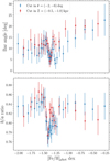 |
Fig. 12 Dependence of the estimated bar angle (top panel) and axis ratio b/a (bottom panel) as a function of metallicity for RR Lyrae stars. We included both the angle and b/a measurements for two sets of conditions including cuts in Galactic latitude (blue circles) or Z coordinate (red squares). The values for individual bins are listed in the appendix (see Tables C.1 and C.2). |
7.1 Galactic bulge in 5D: Transverse velocities
In this subsection, we follow the innovative analysis by Du et al. (2020) and examine the rotation of RR Lyrae stars using the transverse velocities calculated with our distances and updated and improved proper motions from the Gaia DR3. As is noted in Sect. 2.2, all of the proper motions for our RR Lyrae sample come from the Gaia astrometric catalog. To assess the reliability of these proper motions, we employed the following three cuts
 (38)
(38)
 (39)
(39)
 (40):
(40):
where the first condition is composed of the vector, V, containing proper motions in right ascension and declination  and their covariance matrix, Σ (with uncertanities
  , and correlation
  ). The covariance matrix was scaled by the RUWE coefficient and diagonalized, yielding a transformed covariance matrix, Σ*, to remove the correlation between proper motions that would otherwise affect the cut in the first condition in Eq. (38). For the ratio between the transformed vector, V* , and covariance matrix, Σ*, we required at least a five σ confidence in the transformed proper motions. The second and third conditions match those in Eq. (4).
To compute transverse velocities, we used the definition for vℓ and vb from Koppelman & Helmi (2021):
 (41)
(41)
 (42)
(42)
 (43)
(43)
where U⊙, V⊙, W⊙ = (11.1, 12.24, 7.25) km s−1 represent the Solar motion (Schönrich et al. 2010) and vLSR = 230 km s−1 is the velocity of the local standard of rest (Eilers et al. 2019). To estimate the transverse velocities and preserve the correlation in conversion from proper motion vectors in equatorial  to Galactic coordinates (µℓ, µb), we constructed for each RR Lyrae star a multivariate normal distribution where the random values were drawn from the covariance matrix that contained products obtained from Gaia. Since we derived distances independently, we chose to assume negligible correlations between astrometric products and our distances. Using the multivariate distribution, we also estimated Cartesian coordinates (with the Sun at (X, Y, Z) = (0,0,0) kpc).
Figures 13 and D.10 show the results for vℓ with respect to the X coordinate below the Galactic plane with individual points representing a different slice in the Galactic latitude. We binned the data in X (seven bins between 5 and 13 kpc, all within |ℓ| < 2 deg) and Galactic latitude (bins from −1 to −10 deg with 1 deg step size) in the top left panels. We see clear signs that the vℓ varies with the Galactic latitude (at the further side of the bulge), yet still lags behind the rotation of the more metalrich population measured by Sanders et al. (2019). A similar effect was also observed using N-body+smooth particle hydrodynamics simulation (Gough-Kelly et al. 2022) where the older population (tracing a weaker bar) was rotating slower than the younger (as expected from kinematic fractionation Debattista et al. 2017). The dispersion of average vl is expected to be high on the foreground and background periphery of the Galactic bulge (the most distant and closest bins), where the signs of rotation would be the strongest. As we move toward the Galactic center (here set at d = 8.2 kpc), any sign of rotation gets weaker and merges with the interloper contamination (halo and disk stars, assuming it is isotropic and thus centered at vℓ = 0 km s−1).
The insets of both aforementioned figures highlight the variation in the Galactic latitude in the foreground and background edges of the Galactic bulge. The distribution of points across different Galactic latitudes could be interpreted as a sign of differential rotation. Here, we want to emphasize that the prominence of this effect strongly depends on the selected bins, particularly the foreground bin at X = 5.67 kpc where the size of this bin changes the trend in Galactic latitude. If we choose a different set of bins, this sign of rotation decreases, but the point closest to the Galactic plane, b = (−2; −1) deg, nearly always remains with the highest vℓ, and the lag behind the vℓ rotation measured with RC stars (Sanders et al. 2019) is always prevalent.
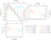 |
Fig. 13 Distribution of vℓ at different distances and Galactic latitudes below the Galactic plane. The top left panel shows the dependence of vℓ on the distance toward the Galactic bulge color-coded according to on different Galactic latitudes. The dashed black line represents the approximate distribution of vℓ from Sanders et al. (2019), and the dotted light blue line represents the distance to the Galactic center. The top right and bottom left panels show insets for two bins from the top left plot, particularly for X bins at 5.67 kpc and 12.33 kpc, respectively, with the same color-coding as in the top left panel. All stars were selected within |ℓ| < 2 deg. For the same figure but for stars above the Galactic plane see Fig. D.10. |
7.2 Metallicity effect
In the following, we examine the transverse velocities as a function of metallicity, similar to the 3D analysis performed in Sect. 6. Figure 14 provides the same RR Lyrae properties (and the same binning in X coordinate) as in the previous figure, Fig. 13, but divided based on photometric metallicities. In this case, we did not bin our data based on Galactic latitude but used all RR Lyrae stars in this analysis. We divided our dataset into two metallicity bins in the same way as in Sect. 6, with [Fe/H] > −1.0 dex, and [Fe/H] < −1.0 dex. We see that the metalrich part of our dataset almost precisely follows the rotation pattern from Sanders et al. (2019) also seen in Du et al. (2020, see their Fig. 7). Particularly on the far side of the Galactic bulge, we see a drastic difference between the rotation of the metalrich and metal-poor RR Lyrae population. On the other hand, the metal-poor part follows the general RR Lyrae trend seen in Fig. 13. In the bottom panel of Fig 14, we see that the dispersion in  decreases for the metal-rich bin but does not reach the values expected from the younger, rotating population. This is probably due to contamination from RR Lyrae stars that are associated with the Galactic disk (see, e.g., Layden et al. 1996; Zinn et al. 2020; Prudil et al. 2020; Iorio & Belokurov 2021). It is important to note that the increase in
  on the far side of the bulge is likely unphysical, as we would expect symmetry with respect to the Galactic center. This increase is probably due to greater uncertainties in distance measurements and significant errors in proper motions. Additionally, the cone-shaped view of our dataset includes more stars at higher Z on the far side of the bulge, which may lead to a higher inclusion of halo stars.
Similar to Sect. 6, Fig. 14 presents a comparison of results and distances based on visual passbands (E(V − I), and mI mean intensity magnitudes). We utilized the same metallicity bins as before and examined vℓ and  . As in the previous case, metalrich RR Lyrae stars more closely mimic RC stars’ rotation and dispersion patterns than metal-poor ones. From Fig. 14, it is evident that trends in vℓ and
  remain consistent across different distance estimation methods. Thus, the variance between visual and near-IR distance assessments, discussed in Sect. 5, has a negligible impact on the analysis of transverse velocities and rotation trends of RR Lyrae stars toward the Galactic bulge.
In Fig. 15, we present the spatial properties of our RR Lyrae dataset, using color coding to represent the values of vℓ across four metallicity bins. This approach allows us to investigate further how vℓ varies with metallicity. Our observations indicate a clear trend: for metal-poor RR Lyrae stars, there is a discernible decrease in the absolute value of vℓ. This effect is at least partly due to halo interlopers, which can slightly influence the observed rotation signal, as is demonstrated by RR Lyrae kinematics (e.g., Kunder et al. 2020; Olivares Carvajal et al. 2024). In contrast, metal-rich RR Lyrae stars exhibit higher absolute values of vℓ , especially in the expected regions, in the foreground and background to the Galactic bulge.
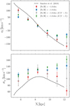 |
Fig. 14 Distribution of vℓ and |

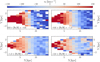 |
Fig. 15 Four panels, divided based on photometric metallicity going from metal-rich to metal-poor RR Lyrae variables, showing the binned spatial distribution in Y vs. X. The color-coding is based on the median value of vℓ in a given bin. The Sun is located at X = 0 and Y = 0 kpc. |
8 Discussion
Since the discovery of a large numbers of RR Lyrae stars toward the Galactic bulge, there has been an ongoing debate over whether these old stars trace the barred bulge or whether they instead belong to a spheroidal inner halo or bulge. The first MACHO survey results showed that the bulge RR Lyrae stars do not follow the barred distribution that the MACHO RC stars show (Minniti et al. 1998). Subsequent MACHO RR Lyrae papers all agreed with this analysis (e.g., Alcock et al. 1998; Kunder & Chaboyer 2008), suggesting the older inner Galaxy RR Lyrae population may have a different origin than the younger bulge. In contrast, the first OGLE survey results showed the bulge RR Lyrae stars do trace a barred distribution (Collinge et al. 2006), and subsequent OGLE RR Lyrae papers continue to find a barred signature in their bulge RR Lyrae samples (e.g., Pietrukowicz et al. 2015). The advent of IR surveys targeting the bulge, particularly the VVV survey, may be able to help resolve this discrepancy. Some IR photometry agrees with the absence of the barred nature of the bulge RR Lyrae stars (Dékány et al. 2013), while other studies argue that the bulge RR Lyrae trace the bar (e.g., Molnar et al. 2022).
The tens of thousands of bulge RR Lyrae stars with precisely measured pulsation properties from OGLE combined with the bulge RR Lyrae stars with near-IR photometry open the possibility of taking a closer look at the effects of the extinction toward the line of sight of the RR Lyrae star. We also can now use new, more precise calibrations of RR Lyrae star PMZ relations that are made possible thanks to Gaia parallaxes as well as improved and homogeneous RR Lyrae metallicities (Bhardwaj et al. 2023; Prudil et al. 2024a) to probe the 3D and 5D spatial distribution of the bulge RR Lyrae stars.
We find that the major cause for the debate surrounding the spatial distribution of the bulge RR Lyrae stars arises from variations in dust properties. A barred RR Lyrae signature naturally arises due to an extinction gradient (mainly in visual passbands) between positive and negative Galactic longitudes, as is shown in Sect. 4. In particular, Figs. 5, D.5, and D.6 illustrate that whereas the specific amplitude of the reddening gradient varies depending on the reddening map used, the overall trend remains consistent. In regions of positive ℓ , extinction calculated from E (V − I) is larger and thus overestimated compared to negative ℓ. This contributes up to a 1 kpc difference in distance estimates based on visual and near-IR passbands, when compared to distances inferred from E (J – Ks) values derived here and in the literature. The reddening gradient seen in E (V – I) disappears when using redder passbands (see the right panels of these figures).
Therefore, in Sect. 5, we show that it is straightforward to recover the bar and its angle from RR Lyrae distances based on visual passbands, but when using distances based on near- IR distances, the bar and its associated tilt are almost negligible (Fig. 7). We quantify the RVI and RJKs deviations in the extinction law across the three different lines of sight. As was expected, the visual spectrum is significantly more impacted (by more than a factor of three) than the IR spectrum. That reddening law variations exist across the bulge is not new (e.g., Nataf et al. 2016, show variations in extinction ratios toward the bulge can exceed 20%), but we show how this directly affects the appearance of the spatial distribution of the inner Galaxy RR Lyrae. Figure 8 demonstrates that the severe variation in the extinction law toward the bulge can be mitigated by employing the reddening law appropriate for the sight-line toward an RR Lyrae star (for example, Table 3 in Nataf et al. 2013). Applying the variations in the interstellar extinction curve reduces the prominence of the bar, but it does not completely remove it for E (V – I).
Attempting to remove the effects of the reddening gradient using corrections based on the reddening maps derived here (E (J – Ks)), we estimate the bar angle ι = 5 ± 2 deg (for our estimates of E (V – I)), resulting in a non-barred spatial distribution of RR Lyrae stars (Fig. 16). However, we do detect the signature of the barred bulge in the more metal-rich RR Lyrae stars ([Fe/H]phot > −1.0 dex) with ι = 18 ± 5 deg, suggesting that not all inner Galaxy RR Lyrae stars belong to the same substructures and therefore suggesting the different epoch of formation of the Milky Way’s bulge. In Fig. 17 we illustrate the extinction variation as a function of Galactic longitude derived from visual and near-IR passbands. Significant fluctuations in both Galactic longitude and latitude are apparent. Specifically, in Galactic longitude, the average change in extinction across the selected regions is about 13%. However, there is a noticeable disparity between positive and negative longitude in the median values. For positive Galactic longitudes, the median variation is smaller, around 9%, while for negative Galactic longitudes, it increases to approximately 16%. Above the Galactic plane, the variation in derived extinction is markedly higher, with median values reaching nearly 50%. This variation is particularly pronounced in the top panel of Fig. 17, where we observe a distinct difference in extinction variation above the Galactic plane between negative and positive ℓ, with the negative values being more significantly affected. Thus, we report a larger extinction variation than the one noted by Sanders et al. (2022). However, in our case, we cover a larger area, both in Galactic longitude and latitude, than in the aforementioned study.
The variations in the extinction law along Galactic longitude and latitude directly contribute to the inconsistent findings regarding the prominence of the bar observed using RR Lyrae variables. Relying on color excess values derived from visual passbands will lead to discrepancies in distance estimates if variations in the reddening law are not taken into account. Although near-IR colors also exhibit variations, these have a smaller impact and are therefore more accommodating to the systematic uncertainties than when using visual passbands.
When examining the transverse kinematics of RR Lyrae variables toward the Galactic bulge, the choice between E (V – I) or E (J – Ks) for distance estimation does not significantly alter the outcomes. Utilizing both approaches, we reach a consistent conclusion: metal-rich RR Lyrae stars demonstrate transverse velocities similar to those estimated using RC stars, as is reported in Sanders et al. (2019), while metal-poor RR Lyrae stars rotate more slowly than RC giants. We shall examine in a future work whether the same holds true for kinematics based on line-of-sight velocities.
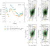 |
Fig. 16 Comparison of spatial distribution estimated through visual passbands in this work (top middle and right panels) and using the method described in Pietrukowicz et al. (2015, marked as P+2015) (bottom middle and right panels) also based partially on visual bands. The top right panel shows a variation in A¡ extinction as a function of the Galactic longitude, estimated using three sources for E (J – Ks) from this work (blue points), form Gonzalez et al. (2012, orange squares), and from Surot et al. (2020, green triangles). The red triangles and blue circles represent two bar angles 20 and 30 degrees, respectively, with shading representing the angles in between. Same as in Fig. 6, the dashed yellow and dotted black lines represent the measured and zero angles, respectively. Lastly, the χ2 of ellipse fits from the top middle panel to the bottom-right hand plot are 0.38, 0.31, 0.25, and 0.18. |
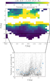 |
Fig. 17 Similar to Fig. 5 but for the ratio between extinction in AI estimated from E (V – I) and E (J – Ks), respectively. |
9 Conclusions
In this study, we have analyzed the spatial and transverse velocity distribution of RR Lyrae stars toward the Galactic bulge. We utilized data from OGLE-IV, Gaia, VVV, and VHS surveys to create reddening maps, derive reddening laws, and estimate distances tailored to each given RR Lyrae variable identified in the Galactic bulge (covering approximately 20 < ℓ < −15 deg and −15 < b < 15 deg area). Our reddening and distances range from visual to near-IR passbands. Using the near-IR passbands, we estimated the distance to the Galactic center as  (stat) ± 528 (sys) pc, after applying a correction for the cone effect. This value is in excellent agreement with measurements from GRAVITY (GRAVITY Collaboration 2019, 2021).
We have examined and confirmed the discrepancy in the spatial distribution observed in inner Galaxy RR Lyrae star studies (e.g., Minniti et al. 1998; Collinge et al. 2006; Kunder & Chaboyer 2008; Dékány et al. 2013; Pietrukowicz et al. 2015). These studies come to different conclusions on whether or not RR Lyrae pulsators trace the bar. After careful examination of the reddening maps and their variation, we believe the main driver behind this inconsistency lies in the variation in the extinction law toward Galactic bulge sight lines. The bar signature in the spatial distribution of RR Lyrae stars disappears in the following cases:
Using a single reddening law for near-IR passbands, E (I – Ks) and E (J – Ks), derived in this study.
By utilizing E (J – Ks) from reddening maps by Gonzalez et al. (2012) and Surot et al. (2020) together with a single reddening law.
For E (V – I) when we apply variations in the reddening law, RVI, for example, measured by Nataf et al. (2013).
We also observe a gradient in extinction differences estimated using visual and near-IR passbands along the Galactic longitudes and latitudes, whereby the former is most likely responsible for the appearance of the bar in spatial properties in visualpassband-based distances.
The purpose of this study is not to measure the extent and angle of the bar, since the density of RR Lyrae stars is lower than that of RC giants. Despite that, we have provided a first-order estimate of the bar angle using distance estimates based on E (J – Ks) for metal-rich RR Lyrae stars ([Fe/H]phot > –1.0 dex), ι = 18 ± 5 deg. This is well within the values estimated in the literature (Bland-Hawthorn & Gerhard 2016, and references therein). The bar’s recovered prominence and angle in the metal-rich RR Lyrae population point tentatively toward it being younger in age (≈10 Gyr) than the bulk of the RR Lyrae bulge population. We also estimated the bar angle as a function of metallicity for our RR Lyrae data using their near-IR distances. We found a clear dependence of the bar angle on metallicity, such that as we move toward the metalrich end of our metallicity distribution, the bar tilt becomes more prominent. A similar trend was observed using Mira variables (e.g., Catchpole et al. 2016; Grady et al. 2020), whereby young Miras exhibit a triaxial distribution, while older Miras show a more spheroidal spatial distribution. Finally, metal-poor RR Lyrae stars ([Fe/H]phot ≤ −1.0 dex) exhibit a smaller bar angle than their metal-rich counterparts. There are two possible explanations for the smaller bar angle observed on the metalpoor side of the RRLyrae metallicity distribution function. First, a high number of interlopers and RRLyrae variables not on barlike orbits could result in a lower estimated bar angle. Second, it might indicate that RR Lyrae stars follow a nearly end-on barred distribution in the Galactic bulge. Resolving these two possibilities will require sufficient systemic velocity measurements for the bulge RRLyrae population, which will be the focus of our next study.
The 5D kinematical analysis relies mainly on the transverse velocities for Galactic longitude. We report that the average velocities derived for RR Lyrae stars lag in rotation compared to average velocities estimated for RC giants (Sanders et al. 2019). Analogously to the 3D analysis, we recover a clear rotation pattern similar to the RC stars for metal-rich RR Lyrae stars ([Fe/H]phot > −1.0 dex). Irrespective of the method used to estimate the distances to the RR Lyrae population in the Galactic bulge, our 5D kinematical results remain the same. This means that despite the variation in extinction law, the conclusions in transverse velocities remain the same both for visual and near-IR-based distance estimates.
For a more conclusive answer to the cause of the lag observed in 5D, we would need to include additional dimensions from the line-of-sight velocities. Moreover, the additional dimension will allow for an analysis of whether metal-poor RR Lyrae variables ([Fe/H]phot < −1.0 dex) exhibit a bar-like tilt and rotation. The full 6D analysis will be the aim of a subsequent study.
Data availability
The full Table C.1 is available at the CDS via anonymous ftp to cdsarc.cds.unistra.fr (130.79.128.5) or via https://cdsarc.cds.unistra.fr/viz-bin/cat/J/A+A/695/A211.
Acknowledgements
Z.P. is grateful to Francesca Fragkoudi, for valuable discussions. LBeS acknowledges the support provided by the Heising Simons Foundation through the Barbara Pichardo Future Faculty Fellowship from grant # 2022-3927. This research made use of the following Python packages: Astropy (Astropy Collaboration 2013, 2018), emcee (Foreman-Mackey et al. 2013), IPython (Pérez & Granger 2007), Matplotlib (Hunter 2007), NumPy (Harris et al. 2020) and SciPy (Virtanen et al. 2020). Z.P. would like to dedicate this work to his daughter, Sofie P.
Appendix A Verification of our distances using Galactic bulge globular clusters
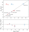 |
Fig. A.1 Comparison of distances derived in this work (based on two reddening laws RVI and |

A comparison of the calculated RR Lyrae distances with globular cluster distances toward the Galactic bulge is depicted in Fig. A.1. We used approximate associations of RR Lyrae stars to globular clusters done by the OGLE team (Soszyński et al. 2014, 2019), their proper motions (using data from the Gaia space telescope Gaia Collaboration 2023, see Sect. 2.2 for more details) together with distances and proper motions from Vasiliev & Baumgardt (2021). We selected those RR Lyrae stars whose proper motions matched the proper motions of globular clusters. We included only those clusters where we could associate at least seven RR Lyrae pulsators (except NGC6453 for passband combination I, GBP −I), and as a distance of a cluster, we selected the weighted average of linked RR Lyrae variables. The listed uncertainties in Table A.1 and displayed in Fig. A.1 represent weighted standard deviations of the given distance distribution.
As a final value for distance to an individual RR Lyrae variable, we preferentially selected measurements derived based on the near-IR passbands Ks band (with E (J − Ks) reddening), or if the J band was not available we used E (I − Ks) reddening. In all other cases, we resort to distances based on I band and E (V − I) or E (GBP − I) reddening, respectively.
Globular clusters toward the Galactic bulge containing a sufficient number of RR Lyrae stars. The first column represents filters used for mean intensity magnitudes and reddening. The second lists globular cluster identifiers. The following two columns contain our derived distance and literature distances and their listed uncertainties. The last column contains the number of RR Lyrae pulsators used in the distance estimate.
Appendix B Oosterhoff dichotomy and the MW bar
The MW globular clusters containing RR Lyrae stars exhibit a bifurcation in periods and metallicities known as the Oosterhoff dichotomy (Oosterhoff 1939, 1944). The RR Lyrae population in the Galactic bulge has been observed to host at least two Oosterhoff groups (see, e.g., Prudil et al. 2019a), which were previously identified and studied among MW globular clusters (see Catelan 2009, for references) and the MW halo (Fabrizio et al. 2019, 2021; Luongo et al. 2024). Recently, it has been shown that estimates of photometric metallicities for RR Lyrae variables associated with the Oosterhoff type II (Oo II) group are less reliable than for those of Oosterhoff type I (Oo I) (see Hajdu et al. 2018; Jurcsik et al. 2021; Jurcsik & Hajdu 2023).
To verify our analysis of the MW bar, we examined the spatial distribution in the X and Y planes for both Oosterhoff types to ensure that our conclusions (e.g., in Sect. 5) regarding the bar prominence remain consistent for both groups. We utilize the technique outlined in (Prudil et al. 2019a) to differentiate between Oosterhoff types for fundamental RR Lyrae pulsators and illustrated their spatial distribution in Fig. B.1 (similar to Figs. 7, 8, and 11), where we presented spatial distributions for Oo I and Oo II groups. We observe that both Oosterhoff groups yielded the same result regarding the bar prominence in RR Lyrae stars. Neither Oo I nor Oo II exhibit an expected tilt with the bar. Therefore, we conclude that RR Lyrae variables associated with the Oo II group offer the same insights despite their less precise photometric metallicities.
We note that the Oo II type RRab stars represent a minority (approximately 17 percent) in our dataset. The reported offset in photometric metallicities (≈0.1 dex Jurcsik et al. 2021) affects the derived distances for the majority of our sample only negligibly due to the use of near-IR passbands (resulting in approximately a 50 pc difference at the distance of the Galactic bulge). This same insignificant impact also applies to the estimates of reddening and extinction for the near-IR photometry. Therefore, the results presented in this work appear to be robust despite the caveats in photometric metallicities for both Oosterhoff groups.
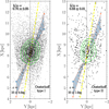 |
Fig. B.1 Spatial distribution of RR Lyrae stars toward the Galactic bulge for Oo I (left panel) and Oo II (right panel) groups, respectively. As in Fig. 6, the measured and zero angles are marked with dashed yellow and dotted black lines, respectively. The quality of the ellipse fit for the left panel is χ2 = 0.25. |
Appendix C Additional tables
Estimated photometric properties in our study. The entire table is provided in the supplementary material for this paper.
| ID | ra | dec | source_id | [Fe/H]phot | ![Mathematical equation: $\sigma _{[{\rm{Fe/H}}]_{{\rm{phot}}} }$](/articles/aa/full_html/2025/03/aa50620-24/aa50620-24-eq128.png) |
 |
 |
ΜJ |  |
ΜI |  |
MV |  |
 |
 |
E (J − Ks) |  |
E (I − Ks) |  |
E (V − I) | σE(V−I) | E (GBP − I) |  |
d | σd |
|---|---|---|---|---|---|---|---|---|---|---|---|---|---|---|---|---|---|---|---|---|---|---|---|---|---|
| – | [deg] | [deg] | – | [dex] | [dex] | [mag] | [mag] | [mag] | [mag] | [mag] | [mag] | [mag] | [mag] | [mag] | [mag] | [mag] | [mag] | [mag] | [mag] | [mag] | [mag] | [mag] | [mag] | [kpc] | [kpc] |
| 00002 | 256.283708 | −32.943917 | 5980012953523019648 | −1.31 | 0.18 | −0.06 | 0.10 | 0.12 | 0.17 | 0.45 | 0.12 | 0.83 | 0.15 | 0.85 | 0.13 | 0.20 | 0.20 | 0.53 | 0.15 | – | – | 0.68 | 0.18 | 8.97 | 0.56 |
| 00003 | 256.291167 | −32.664667 | 5980034497087159424 | −1.34 | 0.07 | −0.31 | 0.09 | −0.07 | 0.17 | 0.31 | 0.11 | 0.76 | 0.14 | 0.78 | 0.13 | 0.28 | 0.19 | 0.66 | 0.15 | – | – | 0.77 | 0.17 | 11.68 | 0.71 |
| 00004 | 256.313417 | −32.837000 | 5980014735918979840 | −1.90 | 0.19 | −0.63 | 0.10 | −0.35 | 0.17 | 0.06 | 0.12 | 0.57 | 0.15 | 0.59 | 0.13 | 0.35 | 0.20 | 0.64 | 0.15 | – | – | 0.79 | 0.18 | 10.42 | 0.66 |
| 00005 | 256.341583 | −32.661806 | 5980035184282597120 | −2.46 | 0.59 | −0.56 | 0.12 | −0.33 | 0.20 | 0.03 | 0.16 | 0.48 | 0.19 | 0.50 | 0.18 | 0.39 | 0.23 | 0.72 | 0.20 | – | – | 0.82 | 0.25 | 7.50 | 0.58 |
| … | … | … | … | … | … | … | … | … | … | … | … | … | … | … | … | … | … | … | … | … | … | … | … | … | … |
Metallicity bins and measured bar angle and axis ratio for RR Lyrae spatial distribution estimated using near-IR passbands (using a condition on b).
Appendix D Additional figures
The additional displayed figures provide the necessary context for estimation of the reddening law (Figs. D.1, D.2, D.3, and D.4), particularly to selected regions in magnitude space for RR Lyrae sample. We also include further analysis of the variation in the reddening law and test of the estimated color-excesses (Figs. D.6, D.8, and D.9). Lastly, we include an analysis of transverse velocities for RR Lyrae variables above the Galactic plane.
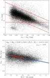 |
Fig. D.1 Color-magnitude diagram (top panel) and linear dependence between color excess E (J − Ks) (lower panel) versus the difference of mean intensity and absolute magnitudes. In the top panel, we plot all sample stars. The red lines denote conditions listed in Table 2 for the selection of bulge RR Lyrae sub-sample. In the bottom panel, the black dots represent selected stars from our sample, blue lines represent the reddening vector, and red circles depict individual bins. |
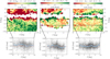 |
Fig. D.5 Same as Fig. 5 but for E (J − Ks) from Surot et al. (2020). |
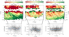 |
Fig. D.6 Same as Fig. 5 but for E (J – Ks) from Gonzalez et al. (2012). |
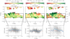 |
Fig. D.7 Same as Fig. 5 but for E (V − I) from Nataf et al. (2013), and E (J − Ks) estimated in this work, and from reddening maps from Surot et al. (2020) and Gonzalez et al. (2012). |
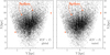 |
Fig. D.8 Spatial distribution of RR Lyrae pulsators in the Cartesian space for two versions of reddening law. The left and right panels show spatial distribution with reddening determined through a single and varied (see Table 4) reddening law, respectively. We note that we used the same dataset as for Fig. 7. The two red dots represent the first and last position of the bar (Gonzalez et al. 2011). |
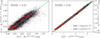 |
Fig. D.9 Comparison of reddening E(J − Ks) (left panel) and E(V − I) (right panel) determined in this study and E(J − Ks) vs E(V − I) obtained based on procedure from Pietrukowicz et al. (2015). The merged dataset used in this section is displayed with black dots. RR Lyrae variables approximately located in the X and Y plane at the position of spikes (see bottom panels of Fig. 7) are marked with red and blue markers. The green line represents the identity line. |
References
- Ablimit, I., Zhao, G., Teklimakan, U., Shi, J.-R., & Abdusalam, K. 2022, ApJS, 258, 20 [NASA ADS] [Google Scholar]
- Alcock, C., Allsman, R. A., Alves, D. R., et al. 1998, ApJ, 492, 190 [NASA ADS] [CrossRef] [Google Scholar]
- Alonso-García, J., Minniti, D., Catelan, M., et al. 2017, ApJ, 849, L13 [Google Scholar]
- Astropy Collaboration (Robitaille, T. P., et al.) 2013, A&A, 558, A33 [NASA ADS] [CrossRef] [EDP Sciences] [Google Scholar]
- Astropy Collaboration (Price-Whelan, A. M., et al.) 2018, AJ, 156, 123 [Google Scholar]
- Athanassoula, E., Rodionov, S. A., & Prantzos, N. 2017, MNRAS, 467, L46 [Google Scholar]
- Barbuy, B., Chiappini, C., & Gerhard, O. 2018, ARA&A, 56, 223 [Google Scholar]
- Bhardwaj, A., Marconi, M., Rejkuba, M., et al. 2023, ApJ, 944, L51 [NASA ADS] [CrossRef] [Google Scholar]
- Binney, J., Gerhard, O. E., Stark, A. A., Bally, J., & Uchida, K. I. 1991, MNRAS, 252, 210 [Google Scholar]
- Bland-Hawthorn, J., & Gerhard, O. 2016, ARA&A, 54, 529 [Google Scholar]
- Blitz, L., & Spergel, D. N. 1991, ApJ, 379, 631 [Google Scholar]
- Bobrick, A., Iorio, G., Belokurov, V., et al. 2024, MNRAS, 527, 12196 [Google Scholar]
- Bono, G., Caputo, F., Castellani, V., et al. 2003, MNRAS, 344, 1097 [Google Scholar]
- Braga, V. F., Stetson, P. B., Bono, G., et al. 2018, AJ, 155, 137 [NASA ADS] [CrossRef] [Google Scholar]
- Braga, V. F., Stetson, P. B., Bono, G., et al. 2019, A&A, 625, A1 [NASA ADS] [CrossRef] [EDP Sciences] [Google Scholar]
- Buck, T., Ness, M., Obreja, A., Macciò, A. V., & Dutton, A. A. 2019, ApJ, 874, 67 [NASA ADS] [CrossRef] [Google Scholar]
- Cao, L., Mao, S., Nataf, D., Rattenbury, N. J., & Gould, A. 2013, MNRAS, 434, 595 [NASA ADS] [CrossRef] [Google Scholar]
- Cardelli, J. A., Clayton, G. C., & Mathis, J. S. 1989, ApJ, 345, 245 [Google Scholar]
- Catchpole, R. M., Whitelock, P. A., Feast, M. W., et al. 2016, MNRAS, 455, 2216 [NASA ADS] [CrossRef] [Google Scholar]
- Catelan, M. 2009, Ap&SS, 320, 261 [Google Scholar]
- Catelan, M., & Smith, H. A. 2015, Pulsating Stars (New York: Wiley) [Google Scholar]
- Catelan, M., Pritzl, B. J., & Smith, H. A. 2004, ApJS, 154, 633 [Google Scholar]
- Chadid, M., Sneden, C., & Preston, G. W. 2017, ApJ, 835, 187 [Google Scholar]
- Clarke, J. P., Wegg, C., Gerhard, O., et al. 2019, MNRAS, 489, 3519 [Google Scholar]
- Clementini, G., Ripepi, V., Garofalo, A., et al. 2023, A&A, 674, A18 [NASA ADS] [CrossRef] [EDP Sciences] [Google Scholar]
- Collinge, M. J., Sumi, T., & Fabrycky, D. 2006, ApJ, 651, 197 [NASA ADS] [CrossRef] [Google Scholar]
- Combes, F., & Sanders, R. H. 1981, A&A, 96, 164 [NASA ADS] [Google Scholar]
- Combes, F., Debbasch, F., Friedli, D., & Pfenniger, D. 1990, A&A, 233, 82 [NASA ADS] [Google Scholar]
- Crestani, J., Braga, V. F., Fabrizio, M., et al. 2021a, ApJ, 914, 10 [NASA ADS] [CrossRef] [Google Scholar]
- Crestani, J., Fabrizio, M., Braga, V. F., et al. 2021b, ApJ, 908, 20 [Google Scholar]
- Cusano, F., Moretti, M. I., Clementini, G., et al. 2021, MNRAS, 504, 1 [NASA ADS] [CrossRef] [Google Scholar]
- Cutri, R. M., Skrutskie, M. F., van Dyk, S., et al. 2003, VizieR Online Data Catalog: II/246 [Google Scholar]
- Debattista, V. P., Carollo, C. M., Mayer, L., & Moore, B. 2004, ApJ, 604, L93 [NASA ADS] [CrossRef] [Google Scholar]
- Debattista, V. P., Mayer, L., Carollo, C. M., et al. 2006, ApJ, 645, 209 [Google Scholar]
- Debattista, V. P., Ness, M., Gonzalez, O. A., et al. 2017, MNRAS, 469, 1587 [Google Scholar]
- Dékány, I., & Grebel, E. K. 2020, ApJ, 898, 46 [CrossRef] [Google Scholar]
- Dékány, I., & Grebel, E. K. 2022, ApJS, 261, 33 [CrossRef] [Google Scholar]
- Dékány, I., Minniti, D., Catelan, M., et al. 2013, ApJ, 776, L19 [Google Scholar]
- Dékány, I., Grebel, E. K., & Pojmański, G. 2021, ApJ, 920, 33 [CrossRef] [Google Scholar]
- Du, H., Mao, S., Athanassoula, E., Shen, J., & Pietrukowicz, P. 2020, MNRAS, 498, 5629 [CrossRef] [Google Scholar]
- Dwek, E., Arendt, R. G., Hauser, M. G., et al. 1995, ApJ, 445, 716 [CrossRef] [Google Scholar]
- Eilers, A.-C., Hogg, D. W., Rix, H.-W., & Ness, M. K. 2019, ApJ, 871, 120 [Google Scholar]
- Fabrizio, M., Bono, G., Braga, V. F., et al. 2019, ApJ, 882, 169 [Google Scholar]
- Fabrizio, M., Braga, V. F., Crestani, J., et al. 2021, ApJ, 919, 118 [NASA ADS] [CrossRef] [Google Scholar]
- Fiorentino, G., Contreras Ramos, R., Tolstoy, E., Clementini, G., & Saha, A. 2012, A&A, 539, A138 [NASA ADS] [CrossRef] [EDP Sciences] [Google Scholar]
- Fiorentino, G., Bono, G., Monelli, M., et al. 2015, ApJ, 798, L12 [Google Scholar]
- For, B.-Q., Sneden, C., & Preston, G. W. 2011, ApJS, 197, 29 [Google Scholar]
- Foreman-Mackey, D., Hogg, D. W., Lang, D., & Goodman, J. 2013, PASP, 125, 306 [Google Scholar]
- Fragkoudi, F., Di Matteo, P., Haywood, M., et al. 2017, A&A, 606, A47 [NASA ADS] [CrossRef] [EDP Sciences] [Google Scholar]
- Fragkoudi, F., Di Matteo, P., Haywood, M., et al. 2018, A&A, 616, A180 [NASA ADS] [CrossRef] [EDP Sciences] [Google Scholar]
- Fragkoudi, F., Grand, R. J. J., Pakmor, R., et al. 2020, MNRAS, 494, 5936 [Google Scholar]
- Fux, R. 1999, A&A, 345, 787 [NASA ADS] [Google Scholar]
- Gaia Collaboration (Brown, A. G. A., et al.) 2016a, A&A, 595, A2 [NASA ADS] [CrossRef] [EDP Sciences] [Google Scholar]
- Gaia Collaboration (Prusti, T., et al.) 2016b, A&A, 595, A1 [NASA ADS] [CrossRef] [EDP Sciences] [Google Scholar]
- Gaia Collaboration (Vallenari, A., et al.) 2023, A&A, 674, A1 [NASA ADS] [CrossRef] [EDP Sciences] [Google Scholar]
- Gonzalez, O. A., Rejkuba, M., Minniti, D., et al. 2011, A&A, 534, L14 [NASA ADS] [CrossRef] [EDP Sciences] [Google Scholar]
- Gonzalez, O. A., Rejkuba, M., Zoccali, M., et al. 2012, A&A, 543, A13 [NASA ADS] [CrossRef] [EDP Sciences] [Google Scholar]
- Gonzalez, O. A., Zoccali, M., Vasquez, S., et al. 2015, A&A, 584, A46 [NASA ADS] [CrossRef] [EDP Sciences] [Google Scholar]
- Gough-Kelly, S., Debattista, V. P., Clarkson, W. I., et al. 2022, MNRAS, 509, 4829 [Google Scholar]
- Grady, J., Belokurov, V., & Evans, N. W. 2019, MNRAS, 483, 3022 [NASA ADS] [CrossRef] [Google Scholar]
- Grady, J., Belokurov, V., & Evans, N. W. 2020, MNRAS, 492, 3128 [NASA ADS] [CrossRef] [Google Scholar]
- GRAVITY Collaboration (Abuter, R., et al.) 2019, A&A, 625, L10 [NASA ADS] [CrossRef] [EDP Sciences] [Google Scholar]
- GRAVITY Collaboration (Abuter, R., et al.) 2021, A&A, 647, A59 [NASA ADS] [CrossRef] [EDP Sciences] [Google Scholar]
- Hajdu, G., Dékány, I., Catelan, M., Grebel, E. K., & Jurcsik, J. 2018, ApJ, 857, 55 [Google Scholar]
- Hajdu, G., Dékány, I., Catelan, M., & Grebel, E. K. 2020, Exp. Astron., 49, 217 [Google Scholar]
- Halir, R., & Flusser, J. 1998, in Numerically stable Direct Least Squares Fitting of Ellipses, eds. Visualization, & I. D. M., Proc. Int. Conf. in Central Europe on Computer Graphics, 125 [Google Scholar]
- Hamanowicz, A., Pietrukowicz, P., Udalski, A., et al. 2016, Acta Astron., 66, 197 [NASA ADS] [Google Scholar]
- Harris, C. R., Millman, K. J., van der Walt, S. J., et al. 2020, Nature, 585, 357–362 [NASA ADS] [CrossRef] [Google Scholar]
- Haschke, R., Grebel, E. K., & Duffau, S. 2011, AJ, 141, 158 [NASA ADS] [Google Scholar]
- Hey, D. R., Huber, D., Shappee, B. J., et al. 2023, AJ, 166, 249 [NASA ADS] [CrossRef] [Google Scholar]
- Hunter, J. D. 2007, Comput. Sci. Eng., 9, 90 [NASA ADS] [CrossRef] [Google Scholar]
- Ibata, R. A., Gilmore, G., & Irwin, M. J. 1994, Nature, 370, 194 [Google Scholar]
- Iorio, G., & Belokurov, V. 2021, MNRAS, 502, 5686 [Google Scholar]
- Johnson, C. I., Rich, R. M., Simion, I. T., et al. 2022, MNRAS, 515, 1469 [NASA ADS] [CrossRef] [Google Scholar]
- Jurcsik, J., & Hajdu, G. 2023, MNRAS, 525, 3486 [NASA ADS] [CrossRef] [Google Scholar]
- Jurcsik, J., & Kovacs, G. 1996, A&A, 312, 111 [Google Scholar]
- Jurcsik, J., Hajdu, G., & Juhász, Á. 2021, MNRAS, 505, 2468 [NASA ADS] [CrossRef] [Google Scholar]
- Khoperskov, S., Minchev, I., Steinmetz, M., et al. 2023, arXiv e-prints [arXiv: 2309.07321] [Google Scholar]
- Koppelman, H. H., & Helmi, A. 2021, A&A, 649, A136 [NASA ADS] [CrossRef] [EDP Sciences] [Google Scholar]
- Kunder, A., & Chaboyer, B. 2008, AJ, 136, 2441 [NASA ADS] [CrossRef] [Google Scholar]
- Kunder, A., & Chaboyer, B. 2009, AJ, 137, 4478 [NASA ADS] [Google Scholar]
- Kunder, A., Popowski, P., Cook, K. H., & Chaboyer, B. 2008, AJ, 135, 631 [NASA ADS] [CrossRef] [Google Scholar]
- Kunder, A., Chaboyer, B., & Layden, A. 2010, AJ, 139, 415 [NASA ADS] [Google Scholar]
- Kunder, A., Koch, A., Rich, R. M., et al. 2012, AJ, 143, 57 [NASA ADS] [CrossRef] [Google Scholar]
- Kunder, A., Rich, R. M., Koch, A., et al. 2016, ApJ, 821, L25 [CrossRef] [Google Scholar]
- Kunder, A., Pérez-Villegas, A., Rich, R. M., et al. 2020, AJ, 159, 270 [NASA ADS] [CrossRef] [Google Scholar]
- Kunder, A., Prudil, Z., Skaggs, C., et al. 2024, AJ, 168, 139 [NASA ADS] [Google Scholar]
- Layden, A. C., Hanson, R. B., Hawley, S. L., Klemola, A. R., & Hanley, C. J. 1996, AJ, 112, 2110 [NASA ADS] [CrossRef] [Google Scholar]
- Leung, H. W., Bovy, J., Mackereth, J. T., et al. 2023, MNRAS, 519, 948 [Google Scholar]
- Li, Z., Shen, J., Gerhard, O., & Clarke, J. P. 2022, ApJ, 925, 71 [CrossRef] [Google Scholar]
- Lim, D., Koch-Hansen, A. J., Chung, C., et al. 2021, A&A, 647, A34 [NASA ADS] [CrossRef] [EDP Sciences] [Google Scholar]
- Lindegren, L., Hernández, J., Bombrun, A., et al. 2018, A&A, 616, A2 [NASA ADS] [CrossRef] [EDP Sciences] [Google Scholar]
- Luongo, E., Ripepi, V., Marconi, M., et al. 2024, A&A, 690, L17 [NASA ADS] [CrossRef] [EDP Sciences] [Google Scholar]
- Madore, B. F. 1982, ApJ, 253, 575 [NASA ADS] [CrossRef] [Google Scholar]
- Marconi, M., Coppola, G., Bono, G., et al. 2015, ApJ, 808, 50 [Google Scholar]
- Martinez-Valpuesta, I., & Gerhard, O. 2013, ApJ, 766, L3 [NASA ADS] [CrossRef] [Google Scholar]
- Martinez-Valpuesta, I., & Shlosman, I. 2004, ApJ, 613, L29 [NASA ADS] [Google Scholar]
- Martínez-Vázquez, C. E., Monelli, M., Bono, G., et al. 2015, MNRAS, 454, 1509 [Google Scholar]
- Matsunaga, N., Fukushi, H., & Nakada, Y. 2005, MNRAS, 364, 117 [NASA ADS] [CrossRef] [Google Scholar]
- McMahon, R. G., Banerji, M., Gonzalez, E., et al. 2013, The Messenger, 154, 35 [NASA ADS] [Google Scholar]
- Medina, G. E., Muñoz, R. R., Vivas, A. K., et al. 2018, ApJ, 855, 43 [NASA ADS] [CrossRef] [Google Scholar]
- Merritt, D., & Sellwood, J. A. 1994, ApJ, 425, 551 [NASA ADS] [CrossRef] [Google Scholar]
- Minniti, D., Alcock, C., Alves, D., et al. 1998, in The Central Regions of the Galaxy and Galaxies, 184, ed. Y. Sofue, 123 [NASA ADS] [Google Scholar]
- Minniti, D., Lucas, P. W., Emerson, J. P., et al. 2010, New A, 15, 433 [Google Scholar]
- Molnar, T. A., Sanders, J. L., Smith, L. C., et al. 2022, MNRAS, 509, 2566 [NASA ADS] [Google Scholar]
- Mullen, J. P., Marengo, M., Martínez-Vázquez, C. E., et al. 2022, ApJ, 931, 131 [NASA ADS] [CrossRef] [Google Scholar]
- Nataf, D. M., Gould, A., Fouqué, P., et al. 2013, ApJ, 769, 88 [Google Scholar]
- Nataf, D. M., Gonzalez, O. A., Casagrande, L., et al. 2016, MNRAS, 456, 2692 [Google Scholar]
- Neeley, J. R., Marengo, M., Bono, G., et al. 2017, ApJ, 841, 84 [Google Scholar]
- Ness, M., Freeman, K., Athanassoula, E., et al. 2013, MNRAS, 432, 2092 [NASA ADS] [CrossRef] [Google Scholar]
- Nishiyama, S., Nagata, T., Baba, D., et al. 2005, ApJ, 621, L105 [NASA ADS] [Google Scholar]
- Nishiyama, S., Nagata, T., Kusakabe, N., et al. 2006, ApJ, 638, 839 [Google Scholar]
- Nishiyama, S., Tamura, M., Hatano, H., et al. 2009, ApJ, 696, 1407 [NASA ADS] [CrossRef] [Google Scholar]
- Olivares Carvajal, J., Zoccali, M., De Leo, M., et al. 2024, A&A, 687, A312 [NASA ADS] [CrossRef] [EDP Sciences] [Google Scholar]
- Oosterhoff, P. T. 1939, The Observatory, 62, 104 [NASA ADS] [Google Scholar]
- Oosterhoff, P. T. 1944, Bull. Astron. Inst. Netherlands, 10, 55 [NASA ADS] [Google Scholar]
- Pedregosa, F., Varoquaux, G., Gramfort, A., et al. 2011, J. Mach. Learn. Res., 12, 2825 [Google Scholar]
- Pérez, F., & Granger, B. E. 2007, Comput. Sci. Eng., 9, 21 [Google Scholar]
- Petersen, J. O. 1986, A&A, 170, 59 [NASA ADS] [Google Scholar]
- Pietrukowicz, P., Kozłowski, S., Skowron, J., et al. 2015, ApJ, 811, 113 [Google Scholar]
- Prudil, Z., Dékány, I., Catelan, M., et al. 2019a, MNRAS, 484, 4833 [NASA ADS] [Google Scholar]
- Prudil, Z., Dékány, I., Grebel, E. K., et al. 2019b, MNRAS, 487, 3270 [NASA ADS] [CrossRef] [Google Scholar]
- Prudil, Z., Dékány, I., Grebel, E. K., & Kunder, A. 2020, MNRAS, 492, 3408 [Google Scholar]
- Prudil, Z., Hanke, M., Lemasle, B., et al. 2021, A&A, 648, A78 [NASA ADS] [CrossRef] [EDP Sciences] [Google Scholar]
- Prudil, Z., Koch-Hansen, A. J., Lemasle, B., et al. 2022, A&A, 664, A148 [NASA ADS] [CrossRef] [EDP Sciences] [Google Scholar]
- Prudil, Z., Kunder, A., Dékány, I., & Koch-Hansen, A. J. 2024a, A&A, 684, A176 [NASA ADS] [CrossRef] [EDP Sciences] [Google Scholar]
- Prudil, Z., Smolec, R., Kunder, A., Koch-Hansen, A. J., & Dékány, I. 2024b, A&A, 685, A153 [NASA ADS] [CrossRef] [EDP Sciences] [Google Scholar]
- Pulsoni, C., Gerhard, O., Arnaboldi, M., et al. 2020, A&A, 641, A60 [EDP Sciences] [Google Scholar]
- Qin, W., Nataf, D. M., Zakamska, N., Wood, P. R., & Casagrande, L. 2018, ApJ, 865, 47 [NASA ADS] [CrossRef] [Google Scholar]
- Quillen, A. C. 2002, AJ, 124, 722 [NASA ADS] [CrossRef] [Google Scholar]
- Raha, N., Sellwood, J. A., James, R. A., & Kahn, F. D. 1991, Nature, 352, 411 [Google Scholar]
- Rodriguez-Fernandez, N. J., & Combes, F. 2008, A&A, 489, 115 [CrossRef] [EDP Sciences] [Google Scholar]
- Rojas-Arriagada, A., Zasowski, G., Schultheis, M., et al. 2020, MNRAS, 499, 1037 [Google Scholar]
- Sandage, A. 2004, AJ, 128, 858 [NASA ADS] [CrossRef] [Google Scholar]
- Sanders, J. L., Smith, L., Evans, N. W., & Lucas, P. 2019, MNRAS, 487, 5188 [CrossRef] [Google Scholar]
- Sanders, J. L., Smith, L., González-Fernández, C., Lucas, P., & Minniti, D. 2022, MNRAS, 514, 2407 [CrossRef] [Google Scholar]
- Sarajedini, A., Mancone, C. L., Lauer, T. R., et al. 2009, AJ, 138, 184 [CrossRef] [Google Scholar]
- Savino, A., Koch, A., Prudil, Z., Kunder, A., & Smolec, R. 2020, A&A, 641, A96 [NASA ADS] [CrossRef] [EDP Sciences] [Google Scholar]
- Schlafly, E. F., Meisner, A. M., Stutz, A. M., et al. 2016, ApJ, 821, 78 [NASA ADS] [CrossRef] [Google Scholar]
- Schönrich, R., Binney, J., & Dehnen, W. 2010, MNRAS, 403, 1829 [NASA ADS] [CrossRef] [Google Scholar]
- Sellwood, J. A., & Gerhard, O. 2020, MNRAS, 495, 3175 [Google Scholar]
- Simion, I. T., Belokurov, V., Irwin, M., et al. 2017, MNRAS, 471, 4323 [NASA ADS] [CrossRef] [Google Scholar]
- Skrutskie, M. F., Cutri, R. M., Stiening, R., et al. 2006, AJ, 131, 1163 [NASA ADS] [CrossRef] [Google Scholar]
- Smirnov, A. A., & Sotnikova, N. Y. 2019, MNRAS, 485, 1900 [NASA ADS] [CrossRef] [Google Scholar]
- Smolec, R. 2005, Acta Astron., 55, 59 [NASA ADS] [Google Scholar]
- Sneden, C., Preston, G. W., Chadid, M., & Adamów, M. 2017, ApJ, 848, 68 [Google Scholar]
- Soszyński, I., Udalski, A., Szymański, M. K., et al. 2014, Acta Astron., 64, 177 [NASA ADS] [Google Scholar]
- Soszyński, I., Udalski, A., Wrona, M., et al. 2019, Acta Astron., 69, 321 [Google Scholar]
- Soszyński, I., Pietrukowicz, P., Udalski, A., et al. 2023, Acta Astron., 73, 105 [Google Scholar]
- Stanek, K. Z., Udalski, A., SzymaŃski, M., et al. 1997, ApJ, 477, 163 [NASA ADS] [CrossRef] [Google Scholar]
- Surot, F., Valenti, E., Hidalgo, S. L., et al. 2019, A&A, 629, A1 [NASA ADS] [CrossRef] [EDP Sciences] [Google Scholar]
- Surot, F., Valenti, E., Gonzalez, O. A., et al. 2020, A&A, 644, A140 [NASA ADS] [CrossRef] [EDP Sciences] [Google Scholar]
- Udalski, A., Szymański, M. K., & Szymański, G. 2015, Acta Astron., 65, 1 [NASA ADS] [Google Scholar]
- Vasiliev, E., & Baumgardt, H. 2021, MNRAS, 505, 5978 [NASA ADS] [CrossRef] [Google Scholar]
- Virtanen, P., Gommers, R., Oliphant, T. E., et al. 2020, Nat. Methods, 17, 261 [Google Scholar]
- Vislosky, E., Minchev, I., Khoperskov, S., et al. 2024, MNRAS, 528, 3576 [NASA ADS] [CrossRef] [Google Scholar]
- Walker, A. R., & Terndrup, D. M. 1991, ApJ, 378, 119 [NASA ADS] [CrossRef] [Google Scholar]
- Wang, S., & Chen, X. 2019, ApJ, 877, 116 [Google Scholar]
- Wegg, C., & Gerhard, O. 2013, MNRAS, 435, 1874 [Google Scholar]
- Wegg, C., Gerhard, O., & Portail, M. 2015, MNRAS, 450, 4050 [NASA ADS] [CrossRef] [Google Scholar]
- Wegg, C., Gerhard, O., & Bieth, M. 2019, MNRAS, 485, 3296 [NASA ADS] [CrossRef] [Google Scholar]
- Weiland, J. L., Arendt, R. G., Berriman, G. B., et al. 1994, ApJ, 425, L81 [NASA ADS] [CrossRef] [Google Scholar]
- Wylie, S. M., Clarke, J. P., & Gerhard, O. E. 2022, A&A, 659, A80 [NASA ADS] [CrossRef] [EDP Sciences] [Google Scholar]
- Zemp, M., Gnedin, O. Y., Gnedin, N. Y., & Kravtsov, A. V. 2011, ApJS, 197, 30 [Google Scholar]
- Zhang, M., & Kainulainen, J. 2019, A&A, 632, A85 [NASA ADS] [CrossRef] [EDP Sciences] [Google Scholar]
- Zinn, R., Chen, X., Layden, A. C., & Casetti-Dinescu, D. I. 2020, MNRAS, 492, 2161 [NASA ADS] [CrossRef] [Google Scholar]
- Zoccali, M., & Valenti, E. 2016, PASA, 33, e025 [NASA ADS] [CrossRef] [Google Scholar]
- Zoccali, M., Vasquez, S., Gonzalez, O. A., et al. 2017, A&A, 599, A12 [NASA ADS] [CrossRef] [EDP Sciences] [Google Scholar]
- Zoccali, M., Quezada, C., Contreras Ramos, R., et al. 2024, A&A, 689, A240 [NASA ADS] [CrossRef] [EDP Sciences] [Google Scholar]
Although alternative channels of RR Lyrae formation have been proposed (see Bobrick et al. 2024).
The aforementioned coefficients can be described by the following equations Ri1 = Ai /A1 and φi1 = φi − iφ1, where the Ri1 represent the amplitude ratio, and the φi1 represent differences in phase.
The photometric metallicities are aligned with the metallicity scale introduced by Crestani et al. (2021b). This scale is based on the studies used in its development, including For et al. (2011), Chadid et al. (2017), Sneden et al. (2017), and Crestani et al. (2021b).
The RUWE parameter estimates the quality of the Gaia astrometric solution.
The module can be found here: https://github.com/idekany/correct_vvv_zp
Available at the VISTA Science Archive http://vsa.roe.ac.uk/
Individual uncertainties in the mean intensity magnitudes, pulsation periods, and photometric metallicities.
Uncertanities in the period-absolute magnitude-metallicity relation, relation for the photometric metallicities.
Available at http://basti-iac.oa-teramo.inaf.it/vvvexmap/
The data are available at https://ogle.astrouw.edu.pl/cgi-ogle/getext.py
For interested readers, we provide our fitting code https://github.com/ZdenekPrudil/Ellipse-fitting
Using the formulas from https://mathworld.wolfram.com/Ellipse.html
The uncertainty on the angle was derived by the variation in the X and Y coordinates within their errors.
All Tables
Linear relations and conditions used to remove foreground and background RR Lyrae stars from our dataset for reddening vector estimation.
Estimated reddening laws in this study and the number of RR Lyrae stars (N✶) used for each reddening law.
Globular clusters toward the Galactic bulge containing a sufficient number of RR Lyrae stars. The first column represents filters used for mean intensity magnitudes and reddening. The second lists globular cluster identifiers. The following two columns contain our derived distance and literature distances and their listed uncertainties. The last column contains the number of RR Lyrae pulsators used in the distance estimate.
Metallicity bins and measured bar angle and axis ratio for RR Lyrae spatial distribution estimated using near-IR passbands (using a condition on b).
All Figures
|
Fig. 1 Spatial distribution of our entire dataset. The gray points represent RR Lyrae stars identified by the OGLE survey and in a study by Dékány & Grebel (2020). Green points represent OGLE-identified RR Lyrae stars with VHS photometry. The orange points mark RR Lyrae stars classified by OGLE with the VVV mean intensity magnitudes from Molnar et al. (2022). |
| In the text | |
|
Fig. 2 Comparison of matched RR Lyrae stars in mean intensity magnitude space (top panel) and period-amplitude plane (bottom panel). The gray dots in both panels represent the total cross-matched sample (between our aperture VVV data and sample provided in Molnar et al. 2022), and red points stand for stars where the absolute difference between both mean intensity magnitudes exceeded 0.3 mag. To assess both photometric sources, we listed the mean and standard deviation between both samples (with discrepant RR Lyrae stars removed). The blue line in the top panel represents the identity line. |
| In the text | |
|
Fig. 3 Spatial distribution of color excesses estimated in this study, E (GBP − I), E (V − I), E (I − Ks), and E (J − Ks). Each point represents a given single-mode RR Lyrae star color-coded based on its associated reddening. Note the different color scales in each panel. |
| In the text | |
|
Fig. 4 Distance distribution of |
| In the text | |
|
Fig. 5 Binned spatial distribution (step equal to 0.5 deg) of differences in estimated extinction ∆AI. Each panel depicts the differences between the extinction (AI) estimated from purely optical or near IR-optical color excesses (E (GBP – I), E (V – I) and E (I – Ks)), and the extinction estimated from the E (J – Ks) color excess. The insets focus on an area below the Galactic plane where we binned (blue circles, seventeen steps between −9.5 to 9.5 deg) the ∆AI as a function of ℓ with gray dots representing individual RR Lyrae stars. |
| In the text | |
|
Fig. 6 Example of ellipse fitting (red line) to the spatial distribution of RR Lyrae stars (blue points). We used distances from this study estimated based on E (V – I) (left panel) and E (J – Ks) (right panel) color excesses. The green squares (used to derive ellipse parameters) and purple triangles represent the half-maximum and maximum of the GMM in a given bin (eleven bins between ℓ ≥ −5 and ℓ ≤ 5 deg). The different bar angles are outlined with dashed and dotted solid black lines. The dashed yellow and dotted black lines mark the measured and zero angles, respectively. The fit quality expressed using χ2 are 0.36, and 0.40 for left and right panels, respectively. |
| In the text | |
|
Fig. 7 Spatial distribution of RR Lyrae pulsators used for comparison in the Cartesian space. Individual subplots display different distance estimates based on near-IR (left column), a combination of near-IR and visual, and only visual reddening. The top panels show Cartesian coordinates derived based on distances estimated in this study. The bottom panels display the distances derived based on procedures from Pietrukowicz et al. (2015) (P+2015, bottom right panel) and Molnar et al. (2022) (M+2022, middle and bottom left panel). We also show two tentative bar angles with red triangles (20 degrees) and blue circles (30 degrees) and a shaded region marks the angles in between. Note that the Sun is at X = 0 and Y = 0 kpc. As is depicted in Fig. 6, the measured and zero angles are marked with dashed yellow and dotted black lines. Lastly, the χ2 of each fit from top left to bottom right are: 0.56, 0.57, 0.35, 0.51, 15, and 0.39. |
| In the text | |
|
Fig. 8 Similar to Fig. 7, we depict spatial distribution bulge RR Lyrae variables using absolute and mean intensity magnitudes (in I band) together with different methods to account for extinction toward the Galactic bulge. The top three panels show spatial distributions derived using color excesses calculated in this work. The bottom two panels show the same spatial distributions but for distances estimated using literature reddening maps toward the Galactic bulge (from left to right, Nataf et al. 2013; Surot et al. 2020; Gonzalez et al. 2012). To measure individual bar angles we binned spatial dataset into eleven bins between ℓ ≥ −5 and ℓ ≤ 5 deg). As in Fig. 6 we depict measured and zero angles with dashed yellow and dotted black lines, respectively. The χ2 for each fit from top left to bottom right are 0.39, 3.4, 0.37, 1.6, 1.4, and 0.43. |
| In the text | |
|
Fig. 9 Comparison of AI extinction estimates in two Galactic longitude bins. The red lines and points represent the bin at positive Galactic longitudes, while the blue points and lines represent stars at negative Galactic longitudes. The dashed lines in the histogram represent the difference in AI for near-IR-based color-excesses, while solid lines show the difference for mainly visual passband-based color-excesses. |
| In the text | |
|
Fig. 10 Test of the inertia tensor method for estimating the bar angle (top panel) and the b/a axis ratio (bottom panel) for our simulated dataset. The solid black lines represent the simulated, unrestricted view of the Galactic bar for different values of |
| In the text | |
|
Fig. 11 Spatial distribution analysis for near-IR distances derived using E(J − Ks). The right and left panels show metal-poor ([Fe/H]phot < −1.0 dex) and metal-rich ([Fe/H]phot > −1.0 dex) RR Lyrae variables in our dataset (black dots). Two approximate bar angles (20 and 30 degrees) are shown with red triangles and blue circles, respectively with shading marking the angles in between. Similar to Fig. 6, we show measured and zero angles with dashed yellow and dotted black lines. Lastly, the quality of the ellipse fit for the left panel is χ2 = 0.45. |
| In the text | |
|
Fig. 12 Dependence of the estimated bar angle (top panel) and axis ratio b/a (bottom panel) as a function of metallicity for RR Lyrae stars. We included both the angle and b/a measurements for two sets of conditions including cuts in Galactic latitude (blue circles) or Z coordinate (red squares). The values for individual bins are listed in the appendix (see Tables C.1 and C.2). |
| In the text | |
|
Fig. 13 Distribution of vℓ at different distances and Galactic latitudes below the Galactic plane. The top left panel shows the dependence of vℓ on the distance toward the Galactic bulge color-coded according to on different Galactic latitudes. The dashed black line represents the approximate distribution of vℓ from Sanders et al. (2019), and the dotted light blue line represents the distance to the Galactic center. The top right and bottom left panels show insets for two bins from the top left plot, particularly for X bins at 5.67 kpc and 12.33 kpc, respectively, with the same color-coding as in the top left panel. All stars were selected within |ℓ| < 2 deg. For the same figure but for stars above the Galactic plane see Fig. D.10. |
| In the text | |
|
Fig. 14 Distribution of vℓ and |
| In the text | |
|
Fig. 15 Four panels, divided based on photometric metallicity going from metal-rich to metal-poor RR Lyrae variables, showing the binned spatial distribution in Y vs. X. The color-coding is based on the median value of vℓ in a given bin. The Sun is located at X = 0 and Y = 0 kpc. |
| In the text | |
|
Fig. 16 Comparison of spatial distribution estimated through visual passbands in this work (top middle and right panels) and using the method described in Pietrukowicz et al. (2015, marked as P+2015) (bottom middle and right panels) also based partially on visual bands. The top right panel shows a variation in A¡ extinction as a function of the Galactic longitude, estimated using three sources for E (J – Ks) from this work (blue points), form Gonzalez et al. (2012, orange squares), and from Surot et al. (2020, green triangles). The red triangles and blue circles represent two bar angles 20 and 30 degrees, respectively, with shading representing the angles in between. Same as in Fig. 6, the dashed yellow and dotted black lines represent the measured and zero angles, respectively. Lastly, the χ2 of ellipse fits from the top middle panel to the bottom-right hand plot are 0.38, 0.31, 0.25, and 0.18. |
| In the text | |
|
Fig. 17 Similar to Fig. 5 but for the ratio between extinction in AI estimated from E (V – I) and E (J – Ks), respectively. |
| In the text | |
|
Fig. A.1 Comparison of distances derived in this work (based on two reddening laws RVI and |
| In the text | |
|
Fig. B.1 Spatial distribution of RR Lyrae stars toward the Galactic bulge for Oo I (left panel) and Oo II (right panel) groups, respectively. As in Fig. 6, the measured and zero angles are marked with dashed yellow and dotted black lines, respectively. The quality of the ellipse fit for the left panel is χ2 = 0.25. |
| In the text | |
|
Fig. D.1 Color-magnitude diagram (top panel) and linear dependence between color excess E (J − Ks) (lower panel) versus the difference of mean intensity and absolute magnitudes. In the top panel, we plot all sample stars. The red lines denote conditions listed in Table 2 for the selection of bulge RR Lyrae sub-sample. In the bottom panel, the black dots represent selected stars from our sample, blue lines represent the reddening vector, and red circles depict individual bins. |
| In the text | |
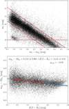 |
Fig. D.2 Same as Fig. D.1 but for I and Ks passbands. |
| In the text | |
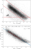 |
Fig. D.3 Same as Fig. D.2 but for V and I passbands. |
| In the text | |
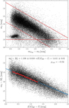 |
Fig. D.4 Same as Fig. D.2 but for GBP and I passbands. |
| In the text | |
|
Fig. D.5 Same as Fig. 5 but for E (J − Ks) from Surot et al. (2020). |
| In the text | |
|
Fig. D.6 Same as Fig. 5 but for E (J – Ks) from Gonzalez et al. (2012). |
| In the text | |
|
Fig. D.7 Same as Fig. 5 but for E (V − I) from Nataf et al. (2013), and E (J − Ks) estimated in this work, and from reddening maps from Surot et al. (2020) and Gonzalez et al. (2012). |
| In the text | |
|
Fig. D.8 Spatial distribution of RR Lyrae pulsators in the Cartesian space for two versions of reddening law. The left and right panels show spatial distribution with reddening determined through a single and varied (see Table 4) reddening law, respectively. We note that we used the same dataset as for Fig. 7. The two red dots represent the first and last position of the bar (Gonzalez et al. 2011). |
| In the text | |
|
Fig. D.9 Comparison of reddening E(J − Ks) (left panel) and E(V − I) (right panel) determined in this study and E(J − Ks) vs E(V − I) obtained based on procedure from Pietrukowicz et al. (2015). The merged dataset used in this section is displayed with black dots. RR Lyrae variables approximately located in the X and Y plane at the position of spikes (see bottom panels of Fig. 7) are marked with red and blue markers. The green line represents the identity line. |
| In the text | |
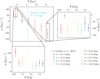 |
Fig. D.10 Same as Fig. 13 but for region above the Galactic plane (b > 0 deg). |
| In the text | |
Current usage metrics show cumulative count of Article Views (full-text article views including HTML views, PDF and ePub downloads, according to the available data) and Abstracts Views on Vision4Press platform.
Data correspond to usage on the plateform after 2015. The current usage metrics is available 48-96 hours after online publication and is updated daily on week days.
Initial download of the metrics may take a while.