| Issue |
A&A
Volume 684, April 2024
|
|
|---|---|---|
| Article Number | A176 | |
| Number of page(s) | 13 | |
| Section | Stellar structure and evolution | |
| DOI | https://doi.org/10.1051/0004-6361/202347338 | |
| Published online | 19 April 2024 | |
The Galactic bulge exploration
I. The period–absolute magnitude–metallicity relations for RR Lyrae stars for GBP, V, G, GRP, I, J, H, and Ks passbands using Gaia DR3 parallaxes
1
Astronomisches Rechen-Institut, Zentrum für Astronomie der Universität Heidelberg, Mönchhofstr. 12-14, 69120 Heidelberg, Germany
2
European Southern Observatory, Karl-Schwarzschild-Strasse 2, 85748 Garching bei München, Germany
e-mail: This email address is being protected from spambots. You need JavaScript enabled to view it.
3
Saint Martin’s University, 5000 Abbey Way SE, Lacey, WA 98503, USA
Received:
3
July
2023
Accepted:
27
October
2023
Abstract
We present a new set of period–absolute magnitude–metallicity (PMZ) relations for single-mode RR Lyrae stars calibrated for the optical GBP, V, G, GRP, near-infrared I, J, H, and Ks passbands. We compiled a large dataset (over 100 objects) of fundamental and first-overtone RR Lyrae pulsators consisting of mean intensity magnitudes, reddenings, pulsation properties, iron abundances, and parallaxes measured by the Gaia astrometric satellite in its third data release. Our newly calibrated PMZ relations encapsulate the most up-to-date ingredients in terms of both data and methodology. They are intended to be used in conjunction with large photometric surveys targeting the Galactic bulge, including the Optical Gravitational Lensing Experiment (OGLE), the Vista Variables in the Vía Láctea Survey (VVV), and the Gaia catalog. In addition, our Bayesian probabilistic approach provides accurate uncertainty estimates of the predicted absolute magnitudes of individual RR Lyrae stars. Our derived PMZ relations provide consistent results when compared to benchmark distances to globular clusters NGC 6121 (also known as M 4), NGC 5139 (also known as omega Cen), and Large and Small Magellanic Clouds, which are stellar systems rich in RR Lyrae stars. Lastly, our Ks-band PMZ relations match well with the previously published PMZ relations based on Gaia data and accurately predict the distance toward the prototype of this class of variables, the eponymic RR Lyr itself.
Key words: methods: data analysis / methods: statistical / parallaxes / stars: variables: RR Lyrae
© The Authors 2024
 Open Access article, published by EDP Sciences, under the terms of the Creative Commons Attribution License (https://creativecommons.org/licenses/by/4.0), which permits unrestricted use, distribution, and reproduction in any medium, provided the original work is properly cited.
This article is published in open access under the Subscribe to Open model. This email address is being protected from spambots. You need JavaScript enabled to view it. to support open access publication.
1. Introduction
RR Lyrae stars are old, helium-burning, mostly radially pulsating horizontal branch giants. They are divided into three main groups based on their pulsation mode: fundamental mode (RRab), first-overtone (RRc), and double-mode pulsators (RRd) pulsating both in fundamental and first-overtone mode. The pulsation properties of all three subclasses have been studied extensively (e.g., Bono et al. 1996; Szabó et al. 2010; Netzel et al. 2015; Smolec et al. 2015; Skarka et al. 2020; Molnár et al. 2022; Netzel & Smolec 2022). The fundamental mode RR Lyrae pulsators often serve as distance and metallicity indicators toward old stellar systems within our Galaxy (e.g., Braga et al. 2015; Skowron et al. 2016; Dékány et al. 2021) and beyond (e.g., Sarajedini et al. 2006, 2009; Fiorentino et al. 2012; Savino et al. 2022).
In particular, the connection between pulsation periods, absolute magnitudes, and metallicities (PMZ relations) of RR Lyrae stars allows us to infer their distances from photometric time series, and it has been one of their most practical features. RR Lyrae PMZ relations have granted opportunities to study structures of old stellar systems (e.g., Dékány et al. 2013; Martínez-Vázquez et al. 2016; Jacyszyn-Dobrzeniecka et al. 2017, 2020) and their distances (e.g., Braga et al. 2015; Martínez-Vázquez et al. 2019; Bhardwaj et al. 2020, 2021; Fabrizio et al. 2021). There are both theoretical and empirical approaches to calibrating the PMZ relations in the literature for various passbands ranging from optical to far-infrared ones (e.g., Bono et al. 2003; Catelan 2004; Neeley et al. 2015, 2017, 2019; Marconi et al. 2015, 2018; Muraveva et al. 2018a; Garofalo et al. 2022).
Empirical studies in the past relied on large samples of RR Lyrae stars (≈400) with metallicities on the Zinn & West (1984) metallicity scale (combining both spectroscopically and photometrically estimated metallicities; e.g., Dambis et al. 2013; Muraveva et al. 2018a; Muhie et al. 2021). The distances in the aforementioned studies were either based on statistical parallax analysis (e.g., Dambis 2009; Dambis et al. 2013) or on trigonometric parallaxes measured by the Gaia space mission (e.g., Muraveva et al. 2018a; Neeley et al. 2019; Layden et al. 2019; Muhie et al. 2021; Garofalo et al. 2022), or, lastly, using distances to RR Lyrae rich globular clusters (e.g., Neeley et al. 2015; Bhardwaj et al. 2021). The photometric information often came from various sources, mainly large photometric surveys covering a broad range of passbands.
In this work, we aim to empirically calibrate the PMZ relations for three major photometric surveys targeting (among others) dense stellar regions in the Milky Way; the Optical Gravitational Lensing Experiment (OGLE, Udalski et al. 2015), the Vista Variables in the Vía Láctea survey (VVV, Minniti et al. 2010), and Gaia astrometric mission (Gaia Collaboration 2016). The combination of these surveys provides optical (OGLE, Gaia) and near-infrared (VVV) photometry for tens of thousands of RR Lyrae stars in crowded stellar regions in the Milky Way. The precise calibration of PMZ relations will allow for accurate distance determination and possible avenues to treat extinction directly based on the color excess of RR Lyrae pulsators. This will enable us to probe the structure of the Galactic bulge from the point of view of old population pulsators (similarly to studies including Dékány et al. 2013; Pietrukowicz et al. 2015; Prudil et al. 2019a; Du et al. 2020), and Molnar et al. (2022) and its kinematical properties (Kunder et al. 2016, 2020; Prudil et al. 2019b; Du et al. 2020).
Previous studies have used both theoretical and empirical PMZ relations to determine distances toward the RR Lyrae population in the Galactic bulge. These relations were not directly calibrated to the photometric systems of OGLE and VVV. They required re-calibration mainly since the OGLE V band is partially different from the standard Johnson V passband (see Udalski et al. 2015) and the VVV JHKs passbands differ from those in the Two-Micron Sky Survey (2MASS, Cutri et al. 2003; Skrutskie et al. 2006). In addition, the metallicity term in the aforementioned PMZ relations was usually calibrated to a different metallicity scale than the estimated metallicities for the bulge RR Lyrae population, thus requiring further conversion (e.g., for Gaia photometry in a study by Muraveva et al. 2018a). Furthermore, previous studies of the Galactic bulge relied mostly on external extinction maps and did not use RR Lyrae stars themselves as tracers of extinction. This motivated the decision to provide PMZ relations that are more appropriate for RR Lyrae stars toward the Galactic bulge. Our subsequent papers will use this calibration to investigate the structure and kinematics of the bulge RR Lyrae population. For the newly derived PMZ relations, we used purely geometrically determined distances by the Gaia astrometric mission (Lindegren et al. 2021; Gaia Collaboration 2023), combined with publicly available data on RR Lyrae stars in the solar neighborhood. In particular, we aimed to use a homogenous metallicity scale among calibrating stars that allows the direct use of photometric metallicities derived from OGLE I-band photometry for RR Lyrae variables toward the Galactic bulge.
This paper is structured as follows. In Sect. 2, we describe our assembled dataset and analysis of the data. The subsequent Sect. 3 outlines our statistical approach to the PMZ calibration and derived equations together with their covariance matrices. In Sect. 4, we test our newly derived relation with the literature values for some of the RR Lyrae-rich stellar systems. Finally, Sect. 5 contains a summary of our results.
2. Dataset for calibration of the PMZ relations
We based our calibration sample on stars with iron abundances presented in Crestani et al. (2021a) and Dékány et al. (2021). Similarly to the calibration by Dékány et al. (2021), individual spectroscopic measurements of [Fe I/H] and [Fe II/H] were collected from the literature and shifted to the common metallicity scale defined by For et al. (2011), Chadid et al. (2017), Sneden et al. (2017), and Crestani et al. (2021b), abbreviated as CFCS, using offsets from Dékány et al. (2021). Each star in our calibration sample had multiple published iron abundance measurements and an associated uncertainty. We obtained the pulsation properties (pulsation period, P) for individual variables in the spectroscopic dataset from various sources, mainly from the International Variable Star Index (VSX, Watson et al. 2006).
Often, pulsation periods are quoted without their appropriate errors; thus, to account for possible minor uncertainties in P, we used the following equation to approximate the uncertainties of pulsation periods σP:
 (1)
(1)
This approach fits σP over an approximate baseline of 1000 days. For a general RRab variable with a pulsation period equal to 0.5 days, Eq. (1) yields σP = 0.001 days. In addition, we converted pulsation periods of the first-overtone (FO) pulsators into fundamental mode using the following equation from Iben (1971) and Braga et al. (2016):
 (2)
(2)
For the entire spectroscopic dataset, values for parallaxes, ϖ, and their uncertainties, σϖ, were obtained from the third data release (DR3) of the Gaia mission (and subsequently corrected for the zero point offset1 by Lindegren et al. 2021). To account for interstellar reddening and to ensure its homogenous treatment, we used 2D extinction maps from Schlegel et al. (1998) to obtain E(B − V) color excesses and its uncertainties toward individual stars and re-calibrated reddening laws from Schlafly & Finkbeiner (2011). The spatial distribution of our spectroscopic dataset in the Galactic coordinates is depicted in Fig. 1.
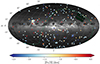 |
Fig. 1. Spatial distribution in Galactic coordinates of our RR Lyrae calibration dataset with color-coding representing an object’s metallicity. Gaia’s all-sky star density map is underpinned in the background (Image credit: Gaia Data Processing and Analysis Consortium (DPAC); A. Moitinho/A. F. Silva/M. Barros/C. Barata, University of Lisbon, Portugal; H. Savietto, Fork Research, Portugal). The overdensity at l ≈ 80 deg and b ≈ 10 deg is due to RR Lyrae stars observed by the Kepler space telescope and followed up spectroscopically by Nemec et al. (2013). |
The intensity magnitudes were obtained from various sources and subsequently transformed into the OGLE and VVV passbands. We emphasize that our RR Lyrae sample sizes vary between the different passbands, and we list the final number of RR Lyrae stars for each calibration after applying quality cuts (see Sect. 3 and Eq. (15)).
In the case of the GBP-, G-, and GRP-band photometry, we utilized the Gaia RR Lyrae catalog with their associated photometric and pulsation properties (Clementini et al. 2023). As the mean intensity magnitudes, mGBP, mG, and mGRP, we used intensity-averaged magnitudes in the aforementioned bands together with their RR Lyrae subclassification, pulsation periods, and uncertainties on pulsation periods. In total, we used 240 (201 RRab and 39 RRc stars) RR Lyrae variables for the GBP, G, and GRP bands, respectively.
For the V passband, we obtained photometry for RR Lyrae stars and subsequently their mean intensity magnitudes, mV, from the All-Sky Automated Survey for Supernovae (ASAS-SN, Shappee et al. 2014; Jayasinghe et al. 2018). This sample contained 166 RR Lyrae stars (136 RRab and 30 RRc pulsators). The same match was conducted for the I-band photometry from Dékány et al. (2021), which yielded 128 RR Lyrae stars in total (104 RRab and 24 RRc pulsators) with mean intensity magnitudes mI. We note that I-band photometry for the calibration RR Lyrae stars came from the predecessor of ASAS-SN, the All Sky Automated Survey (ASAS, Pojmanski 1997; Szczygieł et al. 2009) and was collected from work by Dékány et al. (2021).
The mean intensity magnitudes for V and I-passbands were obtained through Fourier decomposition of photometric light curves using an approach described in Petersen (1986). We optimized the following Fourier light curve decomposition:
 (3)
(3)
In Eq. (3), m represents the mean intensity magnitude and Ak and φk stand for amplitudes and phases. The n denotes the degree of the fit that we adapted for each light curve using the same approach as in Prudil et al. (2019a). The ϑ represents the phase function defined as
 (4)
(4)
where HJD is a heliocentric Julian date representing the time of the observation, and M0 stands for the time of brightness maximum2.
The V and I passbands from the ASAS-SN and ASAS surveys were directly transformed into the OGLE photometric system (Udalski et al. 2015) using common stars between surveys. We used the following linear relations to transform intensity magnitudes:
 (5)
(5)
 (6)
(6)
In the case of the J and H bands, we used the photometry provided by the 2MASS and estimated mean intensity magnitudes, mJ and mH, from Braga et al. (2019). Since 2MASS provides, in most cases, single epoch observations at different pulsation phases, we needed to correct for the luminosity variation during the pulsation cycle to obtain mean intensity magnitudes. For this purpose, we utilized near-infrared photometric templates derived by Braga et al. (2019) in combination with optical, V-band, photometric data from ASAS (to accurately estimate M0 Pojmanski 1997). The choice to use the ASAS data stemmed from the similar time baseline between ASAS and 2MASS, which allowed better constraints on the 2MASS single-epoch observations (pulsation period, time of brightness maxima, amplitude) necessary for template fitting and obtaining the mJ and mH. In the end, we had 115 RR Lyrae stars (97 RRab and 18 RRc variables) with mean intensity magnitudes mJ and 111 RR Lyrae stars (94 RRab and 17 RRc variables) with mean intensity magnitudes mH.
The mean intensity magnitudes in the Ks band were acquired from several sources, particularly from studies by Layden et al. (2019) and Braga et al. (2019). We also used the 2MASS survey, where the same approach as that used for the J and H passbands was used to correct for the luminosity variations as a function of the pulsation cycle. A combination of the studies and surveys mentioned earlier resulted in 155 RR Lyrae stars (129 RRab and 26 RRc variables) with mean intensity magnitudes mKs. The dataset provided by Layden et al. (2019) offered the mean Ks-band magnitudes transformed into the 2MASS photometric system, while photometry from Braga et al. (2019) was also calibrated to the 2MASS photometric system. Therefore, acquired J, H, and Ks mean intensity magnitudes needed to be transformed into the VVV photometric system. We used the equations from the CASU website3 and color terms J − Ks for individual stars to convert our mJ, mH, and mKs magnitudes into the VVV photometric system.
3. Calibration of the PMZ
In this work, we aim to improve the following relation:
![Mathematical equation: $$ \begin{aligned} M = \alpha \,\text{ log}_{10}(P) + \beta \,\text{[Fe/H]} + \gamma , \end{aligned} $$](/articles/aa/full_html/2024/04/aa47338-23/aa47338-23-eq7.gif) (7)
(7)
where M is the absolute magnitude in the given passband (in our study GBP, V, G, GRP, I, J, H, and Ks). The pulsation periods and metallicities are denoted as P and [Fe/H], together with parameters of the PMZ marked as α, β, and γ. Although our dataset is smaller in comparison to previous studies (e.g., Dambis et al. 2013; Muraveva et al. 2018a; Muhie et al. 2021), our calibration is based on a homogeneous metallicity scale that is the same as what is used for the Galactic bulge RR Lyrae stars. This allows for more accurate reddening and distance to be derived, especially in the GBP, V, G, GRP, and I passbands, which are more affected by both reddening and the effect of [Fe/H] metallicity on absolute magnitude. It is important to emphasize that we used both pulsation periods and metallicities to estimate absolute magnitudes for optical (GBP and V) passbands instead of only metallicities as was done in previous studies (e.g., Catelan et al. 2004; Muraveva et al. 2018a). We used both based on a mild anticorrelation (Pearson correlation coefficient equal to −0.47) between pulsation periods and absolute magnitudes (calculated using parallaxes) for both passbands. In addition, the combination of both parameters will decrease uncertainty in the distance, particularly in cases where the metallicity of a given RR Lyrae variable is unknown or highly uncertain.
Our dataset for each passband D consists of vectors dk that contain the following information for individual stars k:
![Mathematical equation: $$ \begin{aligned} \boldsymbol{d}^{k} = \left\{ \text{ log}_{\rm 10}(P), \text{[Fe/H]}, \varpi , m, E(B-V) \right\} ^{k} . \end{aligned} $$](/articles/aa/full_html/2024/04/aa47338-23/aa47338-23-eq8.gif) (8)
(8)
To properly account for errors in our catalog and accurately estimate the PMZ parameters, we employed the following approach utilizing the Bayesian framework where the posterior probability p(θ|D) is equal to:
 (9)
(9)
The θ represents the model parameters θi = {αi,βi,γi,εMi} of the PMZ relation (see Eq. (7)), εMi represents the intrinsic scatter in the PMZ relation, and the p(θ) is the prior probability of the parameter set θ. In our approach, we assumed the prior probability for the intrinsic scatter in the PMZ, εM, that was in the form of a Jeffreys log-uniform prior (Jaynes 1968):
 (10)
(10)
For the α, β, and γ parameters we selected mildly informative uniform priors, 𝒰, based on values from Marconi et al. (2015, see their Table 6 for I, J, H, and Ks). We used the following priors for both the optical GBP, V, G, and GRP bands:
 (11)
(11)
 (12)
(12)
 (13)
(13)
The marginalized likelihood p(D | θ) for k number of stars can be written as such:
 (14)
(14)
The Mdata represents absolute magnitudes estimated using collected photometric and astrometric data. The Mmodel stands for absolute magnitudes estimated through Eq. (7). The 𝒩 represents the normal distribution with a mean μ and standard deviation σ for a variable x, N(x | μ, σ2). In the equations above, Ri denotes the extinction coefficient in a given passband, where we selected a baseline from Cardelli et al. (1989) with RV = 3.1, for individually calibrated passband, we used extinction coefficients from Schlafly & Finkbeiner (2011, for V, I, and Ks), and for the Gaia GBP, G, and GRP-passbands we used the color-dependent extinction coefficients from Gaia Collaboration (2018, see their Eq. (1) and Table 1 for details). The total uncertainty, σMtot, encompassed the individual uncertainties for Mdata, Mmodel, and εMi added in quadrature.
We implemented a set of selection criteria for all involved passbands to ensure we used high-quality data. The general requirements on RR Lyrae stars used for PMZ calibration were that the re-normalized unit weight error (RUWE4) was lower than 1.4, the uncertainty on mean intensity magnitude was σmi < 0.1 mag, and we only used stars outside the highly reddened regions of the MW using the condition |b|> 15 deg. The first and third general conditions prevented the possible problems with astrometric and photometric solutions (e.g., blending). The second condition was primarily applied to remove uncertain mean intensity magnitudes in J. In addition, we implemented two conditions on parallax significance and reddening:
 (15)
(15)
These conditions ensured that we used highly precise parallaxes with stars only weakly affected by reddening. The latter was particularly important for optical passbands where reddening and selecting a reddening law could play a significant role in PMZ calibration.
Using the aforementioned approach and selection criteria, we proceeded to estimate the parameters of the individual PMZ relations. To explore the parameter space, θ, we employed the Markov chain Monte Carlo ensemble sampler implemented in the emcee package by Foreman-Mackey et al. (2013) to maximize the posterior probability defined in the Eq. (9). We ran emcee with 100 walkers for 5000 steps. Using emcee, we thinned the chains by τ = 10 and selected the first 4000 steps as a burn-in, which resulted in 10 000 samples for the posterior distributions. The distribution of θ parameters for the Ks, H, J, I, GRP, G, GBP, and V bands is shown in Figs. 2, A.1–A.7, respectively. The parameters of PMZ relations for eight passbands, together with the total number of variables, N, used in calibration, can be found in the following equations:
![Mathematical equation: $$ \begin{aligned}&M_{K_{s}} = -2.342\,\text{ log}_{10}(P) + 0.138\,\text{[Fe/H]} - 0.801 , N = 97, \end{aligned} $$](/articles/aa/full_html/2024/04/aa47338-23/aa47338-23-eq16.gif) (16)
(16)
![Mathematical equation: $$ \begin{aligned}&M_{H} = -2.250\,\text{ log}_{10}(P) + 0.157\,\text{[Fe/H]} - 0.665 , N = 72,\end{aligned} $$](/articles/aa/full_html/2024/04/aa47338-23/aa47338-23-eq17.gif) (17)
(17)
![Mathematical equation: $$ \begin{aligned}&M_{J} = -1.799\,\text{ log}_{10}(P) + 0.160\,\text{[Fe/H]} - 0.378 , N = 64,\end{aligned} $$](/articles/aa/full_html/2024/04/aa47338-23/aa47338-23-eq18.gif) (18)
(18)
![Mathematical equation: $$ \begin{aligned}&M_{I} = -1.292\,\text{ log}_{10}(P) + 0.196\,\text{[Fe/H]} + 0.197 , N = 79,\end{aligned} $$](/articles/aa/full_html/2024/04/aa47338-23/aa47338-23-eq19.gif) (19)
(19)
![Mathematical equation: $$ \begin{aligned}&M_{G_{\rm RP}} = -1.464\,\text{ log}_{10}(P) + 0.167\,\text{[Fe/H]} + 0.113 , N = 110,\end{aligned} $$](/articles/aa/full_html/2024/04/aa47338-23/aa47338-23-eq20.gif) (20)
(20)
![Mathematical equation: $$ \begin{aligned}&M_{G} = -0.950\,\text{ log}_{10}(P) + 0.202\,\text{[Fe/H]} + 0.614 , N = 110,\end{aligned} $$](/articles/aa/full_html/2024/04/aa47338-23/aa47338-23-eq21.gif) (21)
(21)
![Mathematical equation: $$ \begin{aligned}&M_{V} = -0.582\,\text{ log}_{10}(P) + 0.224\,\text{[Fe/H]} + 0.890 , N = 112,\end{aligned} $$](/articles/aa/full_html/2024/04/aa47338-23/aa47338-23-eq22.gif) (22)
(22)
![Mathematical equation: $$ \begin{aligned}&M_{G_{\rm BP}} = -0.593\,\text{ log}_{10}(P) + 0.228\,\text{[Fe/H]} + 0.913 , N = 107. \end{aligned} $$](/articles/aa/full_html/2024/04/aa47338-23/aa47338-23-eq23.gif) (23)
(23)
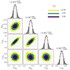 |
Fig. 2. Posterior probability distributions of parameters of PMZ relation for Ks passband. |
Their covariance matrices with associated intrinsic scatter are the following:
 (24)
(24)
 (25)
(25)
 (26)
(26)
 (27)
(27)
 (28)
(28)
 (29)
(29)
 (30)
(30)
 (31)
(31)
In the derived PMZ relations, we see a linear dependence of individual coefficients and passbands. As we move from the near-infrared toward the optical passband, the value of the α coefficient decreases (consequently the importance of pulsation period; Longmore et al. 1986; Dall’Ora et al. 2004) and the value of β increases (the relevance of metallicity). These effects are well known, particularly on the theoretical side, where the near-infrared Ks is shown to have less dependence on metallicity and also less dependence on evolutionary effects (see, e.g., Bono et al. 2003; Catelan et al. 2004; Marconi et al. 2015, 2018). Observations also indicate that there is a decrease in intrinsic scatter when finding MKs (e.g., Neeley et al. 2019; Layden et al. 2019; Cusano et al. 2021).
Together with the assumed intrinsic scatter in the PMZ, εM the absolute magnitude uncertainty calculation for a given RR Lyrae with a parameter vector v = {log10(P),[Fe/H],1.0} is in the following form:
![Mathematical equation: $$ \begin{aligned} \sigma _{M}^{2}&= \mathbf v \times \text{ Cov} \times \boldsymbol{v}^\mathrm{T} + \left[\sigma _{P} \cdot \alpha / \left(P\,\text{ log}\left(10\right)\right) \right]^{2} \nonumber \\&\quad + \left( \beta \cdot \sigma _{\text{[Fe/H]}} \right)^{2} + \varepsilon _{M}^{2}. \end{aligned} $$](/articles/aa/full_html/2024/04/aa47338-23/aa47338-23-eq32.gif) (32)
(32)
Comparisons between absolute magnitude predictions based on our new PMZ relations and estimated absolute magnitudes calculated using Gaia parallaxes and dereddened intensity mean magnitudes are shown in Figs. 3, A.9, A.10, A.12, and A.13.
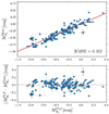 |
Fig. 3. Comparison of absolute magnitudes predicted by our Ks-band PMZ relation with absolute magnitudes calculated based on Gaia data. |
4. Testing predicted absolute magnitudes and comparing PMZ relations
In the following section, we describe how we examined the derived PMZ relations using the publicly available data on stellar systems with precisely derived distances using methods other than RR Lyrae PMZ relations. Also, we compare the derived relation for PMZ in the Ks band with those derived in the literature.
4.1. Predicted absolute magnitudes
We only selected systems with a significant number of RR Lyrae stars and metallicities to test predicted absolute magnitudes on the same metallicity scale as in our PMZ calibration. We picked globular clusters NGC 6121 and NGC 5139 (≡M 4 and ω Centauri, respectively), which have distances and their uncertainties derived using the Gaia parallaxes (Vasiliev & Baumgardt 2021, ϖNGC 6121 = 0.556 ± 0.010 mas and ϖNGC 5139 = 0.193 ± 0.009 mas, respectively). These distances are in agreement within two sigmas with the estimates based on RR Lyrae pulsators (Neeley et al. 2015; Braga et al. 2018). We used available mean intensity magnitudes in optical- and near-infrared passbands from Stetson et al. (2014), Braga et al. (2016), and Braga et al. (2018) and their listed spectroscopic metallicities and pulsation periods when available. In the case of NGC 6121, we used a value for metallicity from the catalog of Carretta et al. (2009) since it is very close to the CFCS scale (difference below −0.1 dex, Crestani et al. 2021b). To account for extinction, we used reddening maps and reddening laws from Schlegel et al. (1998) and Schlafly & Finkbeiner (2011), respectively.
In the case of the Large and Small Magellanic Clouds (from hereon LMC and SMC), we used Gaia and OGLE-IV photometry (GBP, V and I-bands) and stellar classifications from OGLE-IV (Soszyński et al. 2016). We re-analyzed the OGLE photometry using Eq. (3) and estimated photometric metallicities using relations from Dékány et al. (2021), which are on the same scale as our PMZ calibration. For the near-infrared data, we obtained Ks mean intensity magnitudes for 8599 LMC RR Lyrae stars (Cusano et al. 2021) and 473 SMC RR Lyrae pulsators from Muraveva et al. (2018b). For the LMC and SMC distances, we used estimates from Pietrzyński et al. (2019) and Graczyk et al. (2020) based on late-type eclipsing binary stars. For de-reddening the obtained mean intensity magnitudes, we used reddening maps from Schlegel et al. (1998) and reddening laws from Schlafly & Finkbeiner (2011).
We calculated the distance moduli of individual stars and estimated the peak of the distance modulus distribution for each system and passband using the Kernel density estimate routine (KDE; implemented in the Scipy library; Virtanen et al. 2020). The error is estimated as the dispersion of the distance modulus distribution. It is worth noting that this method may not be ideal for the SMC and LMC, as they possess a significant depth extent that can lead to an increased level of measured distance dispersion (e.g., Jacyszyn-Dobrzeniecka et al. 2017; Tatton et al. 2021). In Fig. 4, we compare our PMZ relations with distances to known stellar systems rich in RR Lyrae with sufficient data coverage. In general, the calculated distances using the absolute magnitude relations presented here mostly agree within one σ of the literature distance when using the optical GBP, V, G, GRP, I, and near-infrared J, H, and Ks passbands. The determined distance moduli are listed in Table 1 together with their literature values. In the case of the optical GBP and G bands, we see a significant offset (around 0.2 − 0.25 mag) in distance modulus from the literature value for NGC 6121. This discrepancy is most likely caused by a significant differential reddening toward NGC 6121 (on average E(B − V) = 0.5 mag), the actual proximity of NGC 6121 (2D reddening maps provide only projected reddening), and, in part, color-dependent extinction coefficients for the GBP and G bands. The offset mostly disappears when we use 3D extinction maps (Green 2018; Green et al. 2019). In addition, the offset in the aforementioned optical bands is only observed for NGC 6121. In the other three comparisons, we see a good agreement with the literature distance moduli.
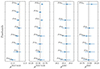 |
Fig. 4. Comparison of distance moduli for four systems (NGC 6121, NGC 5139, LMC, and SMC) with precise distances and uncertainties derived using different methods (other than RR Lyrae PMZ relations; Pietrzyński et al. 2019; Graczyk et al. 2020; Vasiliev & Baumgardt 2021). From the left, the plots show a comparison for globular clusters NGC 6121, NGC 5139, LMC, and SMC using distances and their uncertainties depicted with solid and dotted black lines in all three plots. |
Distance moduli for tested stellar systems using derived PMZ relations.
In conclusion, our optical and near-infrared PMZ relations agree with literature values for NGC 6121, NGC 5139, LMC, and SMC distances. We detected an offset from the canonical values that various effects, for example, reddening, can cause for the GBP and G passbands.
4.2. Comparison with earlier studies
We compare our derived PMZ relation in the Ks band with relations derived in different studies (e.g., Bono et al. 2003; Sollima et al. 2006, 2008; Borissova et al. 2009; Dambis et al. 2013; Muraveva et al. 2015; Bhardwaj et al. 2021, 2023; Muhie et al. 2021). We focused only on the PMZ in the Ks band due to the plethora of derived relations in the literature. We selected relations that combined pulsation periods and metallicities to obtain absolute magnitude in the Ks band.
In the end, we collected 15 relations from the literature for the determination of MKs, derived from both empirical and theoretical approaches. Figure 5 shows a comparison of the literature with the values presented here. Our derived coefficient for the pulsation period, αKs, matches quite well with the overall distribution of literature values. A similar conclusion can be made for the metallicity term, βKs, where despite different metallicity scales used in different studies (e.g., Zinn & West 1984; Carretta et al. 2009) we see a good agreement with the recent studies. Lastly, for the zero point of the PMZ relations, γKs, we see that our derived value agrees exceptionally well with the most recent studies based on Gaia parallaxes despite various sources and scales of metallicity for these studies.
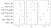 |
Fig. 5. Comparison of coefficients for Ks-passband PMZ relation across different studies (marked with blue crosses, e.g., Bono et al. 2003; Sollima et al. 2006, 2008; Borissova et al. 2009; Dambis et al. 2013; Muraveva et al. 2015; Bhardwaj et al. 2021, 2023; Muhie et al. 2021). Coefficients derived in this work are marked with red points. The green dashed line represents the average of coefficients from previous studies. |
4.3. Comparison with the RR Lyr star
We can compare the results presented here with the prototype of the RR Lyrae class, the RR Lyr itself, since it did not enter our calibration dataset due to its location at low Galactic latitude (b = +12.304 deg, see criteria in Sect. 3). Using the Gaia DR3 zero-point corrected parallax, we derived a geometrical distance d = 249.9 ± 1.9 pc (which is in agreement with distances derived by Bailer-Jones et al. 2021, with d = 249.5 ± 1.5 pc). For comparison, the parallax measured by HIPPARCOS (van Leeuwen 2007) yielded a distance of d = 300 ± 63 pc, and the distance obtained from the parallax measurement by the Hubble Space Telescope was d = 266 ± 9 pc (Benedict et al. 2011). We used 3D extinction map (Green et al. 2019) to obtain a color excess E(B − V) = 0.01 mag5 toward the RR Lyr variable. We decided to compare the PMZ predicted distance to the RR Lyr star only for the Ks-band PMZ relations since it will mitigate the effects of reddening and Ks-band PMZ relations are numerous in the literature. Therefore, we used the 2MASS mean intensity magnitude, mKs, for the RR Lyr variable and corrected it for pulsation motion using photometric templates from Braga et al. (2019). As ephemerides for the RR Lyr, we used data from the GEOS database (Le Borgne et al. 2007), with M0 = 2414921.7746 days and P = 0.566835616 days (Szabó et al. 2014). We took into account that different PMZ relations considered different metallicity scales. Thus, for those that used the Zinn & West (1984) metallicity scale, we used [Fe/H] = −1.37 dex, while for other relations we used [Fe/H] = −1.56 dex.
In Table 2, we list a comparison of the distances for the RR Lyr between different PMZ relations (same as those used in Sect. 4.2). Over half of the PMZ relations overestimate the distance toward the RR Lyr. The scale of overestimation varies from 4 pc up to 26 pc among the different PMZ laws used. Distance differences under 5 pc can be explained by reddening corrections, metallicity variation, and partially by the Gaia parallax offset. The difference between the distance from our derived relation and Gaia is well within one sigma uncertainty of our distance even if we consider only errors on the observed properties (reddening, metallicity, mean intensity magnitude). Here, is important to emphasize the correction of 2MASS mean magnitude for pulsation motion. If we had used the single-epoch 2MASS Ks-band magnitude provided in the 2MASS catalog, we would overestimate the distance toward RR Lyr in nearly all compared PMZ relations. The distance from the PMZ relation would be shifted by approximately 7 pc instead.
Distances for the RR Lyrae star derived using various PMZ relations from the literature.
5. Conclusions
In this work, we calibrated empirical relations that describe the dependence of pulsation periods and metallicities on absolute magnitudes for both fundamental and first-overtone RR Lyrae variables. Our calibration sample was designed to accurately derive PMZ relations for surveys targeting dense stellar structures within the Galaxy. Our study focused on the OGLE, Gaia, and VVV surveys that provide optical and near-infrared photometric observations for many thousands of RR Lyrae stars in the Galactic disk, the Galactic bulge, and in the Magellanic Clouds. Despite our calibration sample being smaller than the ones used in the past, we used a homogeneous metallicity scale that can be easily adapted for RR Lyrae stars in the aforementioned stellar systems.
Our calibration heavily relies on trigonometric parallaxes measured by the Gaia space telescope and the high-resolution metallicities on the CFCS metallicity scale introduced by Crestani et al. (2021b). We considered uncertainties for all involved parameters in our Bayesian approach, including reddening, mean intensity magnitudes, pulsation periods, metallicities, and parallaxes. We also included a parameter for intrinsic scatter in the PMZ in all calibrated passbands to accurately estimate uncertainties in derived absolute magnitudes.
We tested our derived PMZ relations using systems with precise distances and with RR Lyrae stars with publicly available photometry. For optical GBP, near-infrared I, J, and Ks passbands, our relations accurately estimate distance moduli to NGC 6121, NGC 5139, LMC, and SMC. In the case of the optical GBP and G bands for the globular cluster NGC 6121, we detect a significant offset in the derived distance modulus. The offset is mainly caused by the projected reddening and mostly disappears when we use 3D extinction maps toward NGC 6121.
In addition, we compared our predicted Ks-band PMZ relation with previously published relations. Our period and metallicity parameters match well with the overall distribution of literature values (even with relations using a different metalicity scale). The zero-point parameter, on the other hand, matches with PMZ relations based on the Gaia parallaxes. Moreover, we tested the assembled PMZ relation and our derived Ks-band PMZ to estimate the distance toward the prototype of RR Lyrae class, the RR Lyr. We found a good agreement between our derived distance value and distance from Gaia. Our derived PMZ relations will be used in the forthcoming papers to examine the structure and kinematics of the Galactic bulge.
Using a code https://gitlab.com/icc-ub/public/gaiadr3_zeropoint
It is important to note, that the M0 was estimated for each survey separately.
http://casu.ast.cam.ac.uk/surveys-projects/vista/technical/photometric-properties/sky-brightness-variation/view
The RUWE parameter estimates the quality of the Gaia astrometric solution.
Using Schlegel et al. (1998) 2D extinction map, we would obtain E(B − V) = 0.1 mag.
Acknowledgments
Z.P. and A.J.K.H. acknowledge support by the Deutsche Forschungsgemeinschaft (DFG, German Research Foundation) – Project-ID 138713538 – SFB 881 (“The Milky Way System”, subprojects A03, A05, A11). AMK acknowledges support from grant AST-2009836 from the National Science Foundation. This work has made use of data from the European Space Agency (ESA) mission Gaia (https://www.cosmos.esa.int/gaia), processed by the Gaia Data Processing and Analysis Consortium (DPAC, https://www.cosmos.esa.int/web/gaia/dpac/consortium). Funding for the DPAC has been provided by national institutions, in particular the institutions participating in the Gaia Multilateral Agreement. This research made use of the following Python packages: Astropy (Astropy Collaboration 2013, 2018), dustmaps (Green 2018), emcee (Foreman-Mackey et al. 2013), IPython (Pérez & Granger 2007), Matplotlib (Hunter 2007), NumPy (Harris et al. 2020), and SciPy (Virtanen et al. 2020).
References
- Astropy Collaboration (Robitaille, T. P., et al.) 2013, A&A, 558, A33 [NASA ADS] [CrossRef] [EDP Sciences] [Google Scholar]
- Astropy Collaboration (Price-Whelan, A. M., et al.) 2018, AJ, 156, 123 [Google Scholar]
- Bailer-Jones, C. A. L., Rybizki, J., Fouesneau, M., Demleitner, M., & Andrae, R. 2021, AJ, 161, 147 [Google Scholar]
- Benedict, G. F., McArthur, B. E., Feast, M. W., et al. 2011, AJ, 142, 187 [Google Scholar]
- Bhardwaj, A., Rejkuba, M., de Grijs, R., et al. 2020, AJ, 160, 220 [NASA ADS] [CrossRef] [Google Scholar]
- Bhardwaj, A., Rejkuba, M., de Grijs, R., et al. 2021, ApJ, 909, 200 [NASA ADS] [CrossRef] [Google Scholar]
- Bhardwaj, A., Marconi, M., Rejkuba, M., et al. 2023, ApJ, 944, L51 [NASA ADS] [CrossRef] [Google Scholar]
- Bono, G., Caputo, F., Castellani, V., & Marconi, M. 1996, ApJ, 471, L33 [NASA ADS] [CrossRef] [Google Scholar]
- Bono, G., Caputo, F., Castellani, V., et al. 2003, MNRAS, 344, 1097 [Google Scholar]
- Borissova, J., Rejkuba, M., Minniti, D., Catelan, M., & Ivanov, V. D. 2009, A&A, 502, 505 [EDP Sciences] [Google Scholar]
- Braga, V. F., Dall’Ora, M., Bono, G., et al. 2015, ApJ, 799, 165 [NASA ADS] [CrossRef] [Google Scholar]
- Braga, V. F., Stetson, P. B., Bono, G., et al. 2016, AJ, 152, 170 [Google Scholar]
- Braga, V. F., Stetson, P. B., Bono, G., et al. 2018, AJ, 155, 137 [NASA ADS] [CrossRef] [Google Scholar]
- Braga, V. F., Stetson, P. B., Bono, G., et al. 2019, A&A, 625, A1 [NASA ADS] [CrossRef] [EDP Sciences] [Google Scholar]
- Cardelli, J. A., Clayton, G. C., & Mathis, J. S. 1989, ApJ, 345, 245 [Google Scholar]
- Carretta, E., Bragaglia, A., Gratton, R., D’Orazi, V., & Lucatello, S. 2009, A&A, 508, 695 [NASA ADS] [CrossRef] [EDP Sciences] [Google Scholar]
- Catelan, M. 2004, ApJ, 600, 409 [NASA ADS] [CrossRef] [Google Scholar]
- Catelan, M., Pritzl, B. J., & Smith, H. A. 2004, ApJS, 154, 633 [Google Scholar]
- Chadid, M., Sneden, C., & Preston, G. W. 2017, ApJ, 835, 187 [Google Scholar]
- Clementini, G., Ripepi, V., Garofalo, A., et al. 2023, A&A, 674, A18 [NASA ADS] [CrossRef] [EDP Sciences] [Google Scholar]
- Crestani, J., Braga, V. F., Fabrizio, M., et al. 2021a, ApJ, 914, 10 [NASA ADS] [CrossRef] [Google Scholar]
- Crestani, J., Fabrizio, M., Braga, V. F., et al. 2021b, ApJ, 908, 20 [Google Scholar]
- Cusano, F., Moretti, M. I., Clementini, G., et al. 2021, MNRAS, 504, 1 [NASA ADS] [CrossRef] [Google Scholar]
- Cutri, R. M., Skrutskie, M. F., van Dyk, S., et al. 2003, VizieR Online Data Catalog: II/246 [Google Scholar]
- Dall’Ora, M., Storm, J., Bono, G., et al. 2004, ApJ, 610, 269 [Google Scholar]
- Dambis, A. K. 2009, MNRAS, 396, 553 [NASA ADS] [CrossRef] [Google Scholar]
- Dambis, A. K., Berdnikov, L. N., Kniazev, A. Y., et al. 2013, MNRAS, 435, 3206 [Google Scholar]
- Dékány, I., Minniti, D., Catelan, M., et al. 2013, ApJ, 776, L19 [Google Scholar]
- Dékány, I., Grebel, E. K., & Pojmański, G. 2021, ApJ, 920, 33 [CrossRef] [Google Scholar]
- Du, H., Mao, S., Athanassoula, E., Shen, J., & Pietrukowicz, P. 2020, MNRAS, 498, 5629 [CrossRef] [Google Scholar]
- Fabrizio, M., Braga, V. F., Crestani, J., et al. 2021, ApJ, 919, 118 [NASA ADS] [CrossRef] [Google Scholar]
- Fiorentino, G., Contreras Ramos, R., Tolstoy, E., Clementini, G., & Saha, A. 2012, A&A, 539, A138 [NASA ADS] [CrossRef] [EDP Sciences] [Google Scholar]
- For, B.-Q., Sneden, C., & Preston, G. W. 2011, ApJS, 197, 29 [Google Scholar]
- Foreman-Mackey, D., Hogg, D. W., Lang, D., & Goodman, J. 2013, PASP, 125, 306 [Google Scholar]
- Gaia Collaboration (Prusti, T., et al.) 2016, A&A, 595, A1 [NASA ADS] [CrossRef] [EDP Sciences] [Google Scholar]
- Gaia Collaboration (Babusiaux, C., et al.) 2018, A&A, 616, A10 [NASA ADS] [CrossRef] [EDP Sciences] [Google Scholar]
- Gaia Collaboration (Vallenari, A., et al.) 2023, A&A, 674, A1 [NASA ADS] [CrossRef] [EDP Sciences] [Google Scholar]
- Garofalo, A., Delgado, H. E., Sarro, L. M., et al. 2022, MNRAS, 513, 788 [NASA ADS] [CrossRef] [Google Scholar]
- Graczyk, D., Pietrzyński, G., Thompson, I. B., et al. 2020, ApJ, 904, 13 [Google Scholar]
- Green, G. 2018, J. Open Source Softw., 3, 695 [NASA ADS] [CrossRef] [Google Scholar]
- Green, G. M., Schlafly, E., Zucker, C., Speagle, J. S., & Finkbeiner, D. 2019, ApJ, 887, 93 [NASA ADS] [CrossRef] [Google Scholar]
- Harris, C. R., Millman, K. J., van der Walt, S. J., et al. 2020, Nature, 585, 357 [NASA ADS] [CrossRef] [Google Scholar]
- Hunter, J. D. 2007, Comput. Sci. Eng., 9, 90 [NASA ADS] [CrossRef] [Google Scholar]
- Iben, I., Jr., & Huchra, J. 1971, A&A, 14, 293 [NASA ADS] [Google Scholar]
- Jacyszyn-Dobrzeniecka, A. M., Skowron, D. M., Mróz, P., et al. 2017, Acta Astron., 67, 1 [NASA ADS] [Google Scholar]
- Jacyszyn-Dobrzeniecka, A. M., Mróz, P., Kruszyńska, K., et al. 2020, ApJ, 889, 26 [Google Scholar]
- Jayasinghe, T., Kochanek, C. S., Stanek, K. Z., et al. 2018, MNRAS, 477, 3145 [Google Scholar]
- Jaynes, E. T. 1968, IEEE Trans. Syst. Sci. Cybernet., 4, 227 [CrossRef] [Google Scholar]
- Kunder, A., Rich, R. M., Koch, A., et al. 2016, ApJ, 821, L25 [CrossRef] [Google Scholar]
- Kunder, A., Pérez-Villegas, A., Rich, R. M., et al. 2020, AJ, 159, 270 [NASA ADS] [CrossRef] [Google Scholar]
- Layden, A. C., Tiede, G. P., Chaboyer, B., Bunner, C., & Smitka, M. T. 2019, AJ, 158, 105 [NASA ADS] [CrossRef] [Google Scholar]
- Le Borgne, J. F., Paschke, A., Vandenbroere, J., et al. 2007, A&A, 476, 307 [EDP Sciences] [Google Scholar]
- Lindegren, L., Bastian, U., Biermann, M., et al. 2021, A&A, 649, A4 [EDP Sciences] [Google Scholar]
- Longmore, A. J., Fernley, J. A., & Jameson, R. F. 1986, MNRAS, 220, 279 [NASA ADS] [Google Scholar]
- Marconi, M., Coppola, G., Bono, G., et al. 2015, ApJ, 808, 50 [Google Scholar]
- Marconi, M., Bono, G., Pietrinferni, A., et al. 2018, ApJ, 864, L13 [Google Scholar]
- Martínez-Vázquez, C. E., Stetson, P. B., Monelli, M., et al. 2016, MNRAS, 462, 4349 [CrossRef] [Google Scholar]
- Martínez-Vázquez, C. E., Vivas, A. K., Gurevich, M., et al. 2019, MNRAS, 490, 2183 [Google Scholar]
- Minniti, D., Lucas, P. W., Emerson, J. P., et al. 2010, New Astron., 15, 433 [Google Scholar]
- Molnár, L., Bódi, A., Pál, A., et al. 2022, ApJS, 258, 8 [CrossRef] [Google Scholar]
- Molnar, T. A., Sanders, J. L., Smith, L. C., et al. 2022, MNRAS, 509, 2566 [NASA ADS] [Google Scholar]
- Muhie, T. D., Dambis, A. K., Berdnikov, L. N., Kniazev, A. Y., & Grebel, E. K. 2021, MNRAS, 502, 4074 [NASA ADS] [CrossRef] [Google Scholar]
- Muraveva, T., Palmer, M., Clementini, G., et al. 2015, ApJ, 807, 127 [Google Scholar]
- Muraveva, T., Delgado, H. E., Clementini, G., Sarro, L. M., & Garofalo, A. 2018a, MNRAS, 481, 1195 [Google Scholar]
- Muraveva, T., Subramanian, S., Clementini, G., et al. 2018b, MNRAS, 473, 3131 [Google Scholar]
- Neeley, J. R., Marengo, M., Bono, G., et al. 2015, ApJ, 808, 11 [Google Scholar]
- Neeley, J. R., Marengo, M., Bono, G., et al. 2017, ApJ, 841, 84 [Google Scholar]
- Neeley, J. R., Marengo, M., Freedman, W. L., et al. 2019, MNRAS, 490, 4254 [Google Scholar]
- Nemec, J. M., Cohen, J. G., Ripepi, V., et al. 2013, ApJ, 773, 181 [CrossRef] [Google Scholar]
- Netzel, H., & Smolec, R. 2022, MNRAS, 515, 3439 [NASA ADS] [CrossRef] [Google Scholar]
- Netzel, H., Smolec, R., & Moskalik, P. 2015, MNRAS, 447, 1173 [NASA ADS] [CrossRef] [Google Scholar]
- Pérez, F., & Granger, B. E. 2007, Comput. Sci. Eng., 9, 21 [Google Scholar]
- Petersen, J. O. 1986, A&A, 170, 59 [NASA ADS] [Google Scholar]
- Pietrukowicz, P., Kozłowski, S., Skowron, J., et al. 2015, ApJ, 811, 113 [Google Scholar]
- Pietrzyński, G., Graczyk, D., Gallenne, A., et al. 2019, Nature, 567, 200 [Google Scholar]
- Pojmanski, G. 1997, Acta Astron., 47, 467 [Google Scholar]
- Prudil, Z., Dékány, I., Catelan, M., et al. 2019a, MNRAS, 484, 4833 [NASA ADS] [Google Scholar]
- Prudil, Z., Dékány, I., Grebel, E. K., et al. 2019b, MNRAS, 487, 3270 [NASA ADS] [CrossRef] [Google Scholar]
- Sarajedini, A., Barker, M. K., Geisler, D., Harding, P., & Schommer, R. 2006, AJ, 132, 1361 [NASA ADS] [CrossRef] [Google Scholar]
- Sarajedini, A., Mancone, C. L., Lauer, T. R., et al. 2009, AJ, 138, 184 [CrossRef] [Google Scholar]
- Savino, A., Weisz, D. R., Skillman, E. D., et al. 2022, ApJ, 938, 101 [NASA ADS] [CrossRef] [Google Scholar]
- Schlafly, E. F., & Finkbeiner, D. P. 2011, ApJ, 737, 103 [Google Scholar]
- Schlegel, D. J., Finkbeiner, D. P., & Davis, M. 1998, ApJ, 500, 525 [Google Scholar]
- Shappee, B. J., Prieto, J. L., Grupe, D., et al. 2014, ApJ, 788, 48 [Google Scholar]
- Skarka, M., Prudil, Z., & Jurcsik, J. 2020, MNRAS, 494, 1237 [NASA ADS] [CrossRef] [Google Scholar]
- Skowron, D. M., Soszyński, I., Udalski, A., et al. 2016, Acta Astron., 66, 269 [NASA ADS] [Google Scholar]
- Skrutskie, M. F., Cutri, R. M., Stiening, R., et al. 2006, AJ, 131, 1163 [NASA ADS] [CrossRef] [Google Scholar]
- Smolec, R., Soszyński, I., Udalski, A., et al. 2015, MNRAS, 447, 3756 [Google Scholar]
- Sneden, C., Preston, G. W., Chadid, M., & Adamów, M. 2017, ApJ, 848, 68 [Google Scholar]
- Sollima, A., Cacciari, C., & Valenti, E. 2006, MNRAS, 372, 1675 [Google Scholar]
- Sollima, A., Cacciari, C., Arkharov, A. A. H., et al. 2008, MNRAS, 384, 1583 [Google Scholar]
- Soszyński, I., Udalski, A., Szymański, M. K., et al. 2016, Acta Astron., 66, 131 [NASA ADS] [Google Scholar]
- Stetson, P. B., Braga, V. F., Dall’Ora, M., et al. 2014, PASP, 126, 521 [NASA ADS] [CrossRef] [Google Scholar]
- Szabó, R., Kolláth, Z., Molnár, L., et al. 2010, MNRAS, 409, 1244 [CrossRef] [Google Scholar]
- Szabó, R., Benkő, J. M., Paparó, M., et al. 2014, A&A, 570, A100 [NASA ADS] [CrossRef] [EDP Sciences] [Google Scholar]
- Szczygieł, D. M., Pojmański, G., & Pilecki, B. 2009, Acta Astron., 59, 137 [NASA ADS] [Google Scholar]
- Tatton, B. L., van Loon, J. T., Cioni, M. R. L., et al. 2021, MNRAS, 504, 2983 [NASA ADS] [CrossRef] [Google Scholar]
- Udalski, A., Szymański, M. K., & Szymański, G. 2015, Acta Astron., 65, 1 [NASA ADS] [Google Scholar]
- van Leeuwen, F. 2007, A&A, 474, 653 [CrossRef] [EDP Sciences] [Google Scholar]
- Vasiliev, E., & Baumgardt, H. 2021, MNRAS, 505, 5978 [NASA ADS] [CrossRef] [Google Scholar]
- Virtanen, P., Gommers, R., Oliphant, T. E., et al. 2020, Nat. Methods, 17, 261 [Google Scholar]
- Watson, C. L., Henden, A. A., & Price, A. 2006, Soc. Astron. Sci. Ann. Symp., 25, 47 [NASA ADS] [Google Scholar]
- Zinn, R., & West, M. J. 1984, ApJS, 55, 45 [Google Scholar]
Appendix A: Additional figures
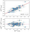 |
Fig. A.10. Same as Fig. 3, but for the I band. |
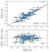 |
Fig. A.11. Same as Fig. 3, but for the GRP band. |
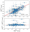 |
Fig. A.12. Same as Fig. 3, but for the G band. |
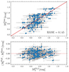 |
Fig. A.13. Same as Fig. 3, but for the V band. |
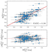 |
Fig. A.14. Same as Fig. 3, but for the GBP band. |
All Tables
Distances for the RR Lyrae star derived using various PMZ relations from the literature.
All Figures
|
Fig. 1. Spatial distribution in Galactic coordinates of our RR Lyrae calibration dataset with color-coding representing an object’s metallicity. Gaia’s all-sky star density map is underpinned in the background (Image credit: Gaia Data Processing and Analysis Consortium (DPAC); A. Moitinho/A. F. Silva/M. Barros/C. Barata, University of Lisbon, Portugal; H. Savietto, Fork Research, Portugal). The overdensity at l ≈ 80 deg and b ≈ 10 deg is due to RR Lyrae stars observed by the Kepler space telescope and followed up spectroscopically by Nemec et al. (2013). |
| In the text | |
|
Fig. 2. Posterior probability distributions of parameters of PMZ relation for Ks passband. |
| In the text | |
|
Fig. 3. Comparison of absolute magnitudes predicted by our Ks-band PMZ relation with absolute magnitudes calculated based on Gaia data. |
| In the text | |
|
Fig. 4. Comparison of distance moduli for four systems (NGC 6121, NGC 5139, LMC, and SMC) with precise distances and uncertainties derived using different methods (other than RR Lyrae PMZ relations; Pietrzyński et al. 2019; Graczyk et al. 2020; Vasiliev & Baumgardt 2021). From the left, the plots show a comparison for globular clusters NGC 6121, NGC 5139, LMC, and SMC using distances and their uncertainties depicted with solid and dotted black lines in all three plots. |
| In the text | |
|
Fig. 5. Comparison of coefficients for Ks-passband PMZ relation across different studies (marked with blue crosses, e.g., Bono et al. 2003; Sollima et al. 2006, 2008; Borissova et al. 2009; Dambis et al. 2013; Muraveva et al. 2015; Bhardwaj et al. 2021, 2023; Muhie et al. 2021). Coefficients derived in this work are marked with red points. The green dashed line represents the average of coefficients from previous studies. |
| In the text | |
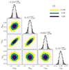 |
Fig. A.1. Same as Fig. 2, but for the H band. |
| In the text | |
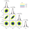 |
Fig. A.2. Same as Fig. 2, but for the J band. |
| In the text | |
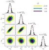 |
Fig. A.3. Same as Fig. 2, but for the I band. |
| In the text | |
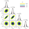 |
Fig. A.4. Same as Fig. 2, but for the GRP band. |
| In the text | |
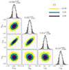 |
Fig. A.5. Same as Fig. 2, but for the G band. |
| In the text | |
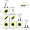 |
Fig. A.6. Same as Fig. 2, but for the V band. |
| In the text | |
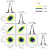 |
Fig. A.7. Same as Fig. 2, but for the GBP band. |
| In the text | |
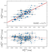 |
Fig. A.8. Same as Fig. 3, but for the J band. |
| In the text | |
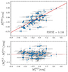 |
Fig. A.9. Same as Fig. 3, but for the J band. |
| In the text | |
|
Fig. A.10. Same as Fig. 3, but for the I band. |
| In the text | |
|
Fig. A.11. Same as Fig. 3, but for the GRP band. |
| In the text | |
|
Fig. A.12. Same as Fig. 3, but for the G band. |
| In the text | |
|
Fig. A.13. Same as Fig. 3, but for the V band. |
| In the text | |
|
Fig. A.14. Same as Fig. 3, but for the GBP band. |
| In the text | |
Current usage metrics show cumulative count of Article Views (full-text article views including HTML views, PDF and ePub downloads, according to the available data) and Abstracts Views on Vision4Press platform.
Data correspond to usage on the plateform after 2015. The current usage metrics is available 48-96 hours after online publication and is updated daily on week days.
Initial download of the metrics may take a while.