| Issue |
A&A
Volume 697, May 2025
Euclid on Sky
|
|
|---|---|---|
| Article Number | A5 | |
| Number of page(s) | 47 | |
| Section | Cosmology (including clusters of galaxies) | |
| DOI | https://doi.org/10.1051/0004-6361/202450853 | |
| Published online | 30 April 2025 | |
Euclid
V. The Flagship galaxy mock catalogue: A comprehensive simulation for the Euclid mission
1
Institute of Space Sciences (ICE, CSIC), Campus UAB, Carrer de Can Magrans, s/n,
08193
Barcelona,
Spain
2
Institut d’Estudis Espacials de Catalunya (IEEC), Edifici RDIT, Campus UPC,
08860
Castelldefels, Barcelona,
Spain
3
Department of Astrophysics, University of Zurich,
Winterthurerstrasse 190,
8057
Zurich, Switzerland
4
Centro de Investigaciones Energéticas, Medioambientales y Tecnológicas (CIEMAT),
Avenida Complutense 40,
28040
Madrid, Spain
5
Port d’Informació Científica, Campus UAB,
C. Albareda s/n,
08193
Bellaterra (Barcelona), Spain
6
INAF-Osservatorio di Astrofisica e Scienza dello Spazio di Bologna,
Via Piero Gobetti 93/3,
40129
Bologna, Italy
7
Institut d’Astrophysique de Paris, UMR 7095, CNRS, and Sorbonne Université,
98 bis boulevard Arago,
75014
Paris,
France
8
Institut d’Astrophysique de Paris,
98bis Boulevard Arago,
75014,
Paris,
France
9
Kavli Institute for the Physics and Mathematics of the Universe (WPI), University of Tokyo,
Kashiwa, Chiba
277-8583, Japan
10
Laboratoire Univers et Théorie, Observatoire de Paris, Université PSL, Université Paris Cité, CNRS,
92190
Meudon,
France
11
Instituto de Astrofísica de Canarias,
Calle Vía Láctea s/n,
38204,
San Cristóbal de La Laguna, Tenerife,
Spain
12
Instituto de Astrofísica de Canarias (IAC); Departamento de Astrofísica, Universidad de La Laguna (ULL),
38200,
La Laguna,
Tenerife, Spain
13
Université PSL, Observatoire de Paris, Sorbonne Université, CNRS, LERMA,
75014,
Paris, France
14
Université Paris-Cité,
5 Rue Thomas Mann,
75013,
Paris, France
15
Dipartimento di Fisica - Sezione di Astronomia, Università di Trieste,
Via Tiepolo 11,
34131
Trieste, Italy
16
INAF-Osservatorio Astronomico di Trieste,
Via G. B. Tiepolo 11,
34143
Trieste, Italy
17
INFN, Sezione di Trieste,
Via Valerio 2,
34127
Trieste TS, Italy
18
IFPU, Institute for Fundamental Physics of the Universe,
via Beirut 2,
34151
Trieste, Italy
19
Institut de Física d’Altes Energies (IFAE), The Barcelona Institute of Science and Technology, Campus UAB,
08193
Bellaterra (Barcelona), Spain
20
Instituto de Astronomia Teorica y Experimental (IATE-CONICET),
Laprida 854,
X5000BGR,
Córdoba,
Argentina
21
Minnesota Institute for Astrophysics, University of Minnesota,
116 Church St SE,
Minneapolis,
MN
55455, USA
22
Institut de Ciencies de l’Espai (IEEC-CSIC), Campus UAB, Carrer de Can Magrans,
s/n Cerdanyola del Vallés,
08193
Barcelona,
Spain
23
Universität Innsbruck, Institut für Astro- und Teilchenphysik,
Technikerstr. 25/8,
6020
Innsbruck, Austria
24
Leiden Observatory, Leiden University,
Einsteinweg 55,
2333
CC Leiden, The Netherlands
25
Department of Astronomy, School of Physics and Astronomy, Shanghai Jiao Tong University,
Shanghai
200240, China
26
Shanghai Key Laboratory for Particle Physics and Cosmology,
Shanghai
200240, China
27
Waterloo Centre for Astrophysics, University of Waterloo,
Waterloo,
Ontario
N2L 3G1, Canada
28
Department of Physics and Astronomy, University of Waterloo,
Waterloo,
Ontario
N2L 3G1, Canada
29
INFN Gruppo Collegato di Parma,
Viale delle Scienze 7/A
43124
Parma, Italy
30
SISSA, International School for Advanced Studies,
Via Bonomea 265,
34136
Trieste TS, Italy
31
International Centre for Theoretical Physics (ICTP),
Strada Costiera 11,
34151
Trieste, Italy
32
Department of Astrophysical Sciences, Peyton Hall, Princeton University,
Princeton,
NJ
08544, USA
33
Institut de Recherche en Astrophysique et Planétologie (IRAP), Université de Toulouse, CNRS, UPS, CNES,
14 Av. Edouard Belin,
31400
Toulouse,
France
34
Department of Physics, Oxford University,
Keble Road,
Oxford
OX1 3RH, UK
35
Institute for Astronomy, University of Edinburgh, Royal Observatory,
Blackford Hill,
Edinburgh
EH9 3HJ, UK
36
Institute of Physics, Laboratory for Galaxy Evolution, Ecole Polytechnique Fédérale de Lausanne, Observatoire de Sauverny,
1290
Versoix,
Switzerland
37
Max Planck Institute for Extraterrestrial Physics,
Giessenbachstr. 1,
85748
Garching, Germany
38
Université Paris-Saclay, Université Paris Cité, CEA, CNRS, AIM,
91191,
Gif-sur-Yvette, France
39
Mullard Space Science Laboratory, University College London, Holmbury St Mary,
Dorking, Surrey
RH5 6NT, UK
40
Perimeter Institute for Theoretical Physics,
Waterloo,
Ontario
N2L 2Y5, Canada
41
Dipartimento di Fisica “Aldo Pontremoli”, Università degli Studi di Milano,
Via Celoria 16,
20133
Milano, Italy
42
INAF-Osservatorio Astronomico di Brera,
Via Brera 28,
20122
Milano, Italy
43
Department of Astronomy, University of Geneva,
ch. d’Ecogia 16,
1290
Versoix, Switzerland
44
Niels Bohr Institute, University of Copenhagen,
Jagtvej 128,
2200
Copenhagen, Denmark
45
Cosmic Dawn Center (DAWN),
Denmark
46
Jodrell Bank Centre for Astrophysics, Department of Physics and Astronomy, University of Manchester,
Oxford Road,
Manchester
M13 9PL, UK
47
INAF-Osservatorio Astronomico di Capodimonte,
Via Moiariello 16,
80131
Napoli, Italy
48
Departamento de Física Teórica, Facultad de Ciencias, Universidad Autónoma de Madrid,
28049
Cantoblanco, Madrid,
Spain
49
Serra Húnter Fellow, Departament de Física, Universitat Autònoma de Barcelona,
E-08193
Bellaterra, Spain
50
Konkoly Observatory, HUN-REN CSFK, MTA Centre of Excellence,
Budapest,
Konkoly Thege Miklós út 15-17.
1121,
Hungary
51
MTA-CSFK Lendület Large-Scale Structure Research Group,
Konkoly-Thege Miklós út 15-17,
1121
Budapest, Hungary
52
Université Paris-Saclay, CNRS, Institut d’astrophysique spatiale,
91405,
Orsay,
France
53
ESAC/ESA, Camino Bajo del Castillo,
s/n., Urb. Villafranca del Castillo,
28692
Villanueva de la Cañada, Madrid,
Spain
54
School of Mathematics and Physics, University of Surrey,
Guildford, Surrey,
GU2 7XH,
UK
55
Institut für Theoretische Physik, University of Heidelberg,
Philosophenweg 16,
69120
Heidelberg, Germany
56
Dipartimento di Fisica e Astronomia, Università di Bologna,
Via Gobetti 93/2,
40129
Bologna, Italy
57
INFN-Sezione di Bologna,
Viale Berti Pichat 6/2,
40127
Bologna, Italy
58
INAF-Osservatorio Astronomico di Padova,
Via dell’Osservatorio 5,
35122
Padova, Italy
59
Universitäts-Sternwarte München, Fakultät für Physik, Ludwig-Maximilians-Universität München,
Scheinerstrasse 1,
81679
München, Germany
60
Institut de Physique Théorique, CEA, CNRS, Université Paris-Saclay
91191
Gif-sur-Yvette Cedex, France
61
INAF-Osservatorio Astrofisico di Torino,
Via Osservatorio 20,
10025
Pino Torinese (TO), Italy
62
Dipartimento di Fisica, Università di Genova,
Via Dodecaneso 33,
16146,
Genova,
Italy
63
INFN-Sezione di Genova,
Via Dodecaneso 33,
16146,
Genova,
Italy
64
Department of Physics “E. Pancini”, University Federico II,
Via Cinthia 6,
80126,
Napoli,
Italy
65
INFN section of Naples,
Via Cinthia 6,
80126,
Napoli,
Italy
66
Instituto de Astrofísica e Ciências do Espaço, Universidade do Porto, CAUP,
Rua das Estrelas,
PT4150-762
Porto, Portugal
67
Faculdade de Ciências da Universidade do Porto,
Rua do Campo de Alegre,
4150-007
Porto, Portugal
68
Dipartimento di Fisica, Università degli Studi di Torino,
Via P. Giuria 1,
10125
Torino, Italy
69
INFN-Sezione di Torino,
Via P. Giuria 1,
10125
Torino, Italy
70
INAF-IASF Milano,
Via Alfonso Corti 12,
20133
Milano, Italy
71
Institute for Theoretical Particle Physics and Cosmology (TTK), RWTH Aachen University,
52056
Aachen,
Germany
72
INAF-Osservatorio Astronomico di Roma,
Via Frascati 33,
00078
Monteporzio Catone, Italy
73
Dipartimento di Fisica e Astronomia “Augusto Righi” – Alma Mater Studiorum Università di Bologna,
Viale Berti Pichat 6/2,
40127
Bologna, Italy
74
European Space Agency/ESRIN,
Largo Galileo Galilei 1,
00044 Frascati, Roma,
Italy
75
Université Claude Bernard Lyon 1, CNRS/IN2P3, IP2I Lyon, UMR 5822,
Villeurbanne,
F-69100, France
76
Institute of Physics, Laboratory of Astrophysics, Ecole Polytechnique Fédérale de Lausanne (EPFL), Observatoire de Sauverny,
1290
Versoix,
Switzerland
77
UCB Lyon 1, CNRS/IN2P3, IUF, IP2I Lyon,
4 rue Enrico Fermi,
69622
Villeurbanne,
France
78
Departamento de Física, Faculdade de Ciências, Universidade de Lisboa, Edifício C8, Campo Grande,
PT1749-016
Lisboa, Portugal
79
Instituto de Astrofísica e Ciências do Espaço, Faculdade de Ciências, Universidade de Lisboa, Campo Grande,
1749-016
Lisboa, Portugal
80
INAF-Istituto di Astrofisica e Planetologia Spaziali,
via del Fosso del Cavaliere, 100,
00100
Roma, Italy
81
INFN-Padova,
Via Marzolo 8,
35131
Padova, Italy
82
School of Physics, HH Wills Physics Laboratory, University of Bristol,
Tyndall Avenue,
Bristol,
BS8 1TL,
UK
83
Aix-Marseille Université, CNRS/IN2P3, CPPM,
Marseille,
France
84
Istituto Nazionale di Fisica Nucleare, Sezione di Bologna,
Via Irnerio 46,
40126
Bologna, Italy
85
FRACTAL S.L.N.E.,
calle Tulipán 2, Portal 13 1A,
28231,
Las Rozas de Madrid, Spain
86
Institute of Theoretical Astrophysics, University of Oslo,
PO Box 1029
Blindern, 0315
Oslo,
Norway
87
Jet Propulsion Laboratory, California Institute of Technology,
4800 Oak Grove Drive,
Pasadena,
CA,
91109,
USA
88
Department of Physics, Lancaster University,
Lancaster,
LA1 4YB,
UK
89
Felix Hormuth Engineering,
Goethestr. 17,
69181
Leimen, Germany
90
Technical University of Denmark,
Elektrovej 327,
2800 Kgs.
Lyngby, Denmark
91
Université Paris-Saclay, CNRS/IN2P3, IJCLab,
91405
Orsay,
France
92
Max-Planck-Institut für Astronomie,
Königstuhl 17,
69117
Heidelberg, Germany
93
NASA Goddard Space Flight Center,
Greenbelt,
MD
20771, USA
94
Department of Physics and Astronomy, University College London,
Gower Street,
London
WC1E 6BT, UK
95
Department of Physics and Helsinki Institute of Physics,
Gustaf Hällströmin katu 2,
00014 University of Helsinki,
Finland
96
Université de Genève, Département de Physique Théorique and Centre for Astroparticle Physics,
24 quai Ernest-Ansermet,
1211
Genève 4, Switzerland
97
Department of Physics,
P.O. Box 64,
00014 University of Helsinki,
Finland
98
Helsinki Institute of Physics,
Gustaf Hällströmin katu 2,
University of Helsinki, Helsinki,
Finland
99
European Space Agency/ESTEC,
Keplerlaan 1,
2201 AZ
Noordwijk, The Netherlands
100
Aix-Marseille Université, CNRS, CNES, LAM,
Marseille,
France
101
NOVA optical infrared instrumentation group at ASTRON,
Oude Hoogeveensedijk 4,
7991PD,
Dwingeloo,
The Netherlands
102
INFN-Sezione di Milano,
Via Celoria 16,
20133
Milano, Italy
103
University of Applied Sciences and Arts of Northwestern Switzerland, School of Engineering,
5210
Windisch,
Switzerland
104
Universität Bonn, Argelander-Institut für Astronomie,
Auf dem Hügel 71,
53121
Bonn, Germany
105
INFN-Sezione di Roma,
Piazzale Aldo Moro 2, c/o Dipartimento di Fisica, Edificio G. Marconi,
00185
Roma,
Italy
106
Dipartimento di Fisica e Astronomia “Augusto Righi” – Alma Mater Studiorum Università di Bologna,
via Piero Gobetti 93/2,
40129
Bologna, Italy
107
Department of Physics, Institute for Computational Cosmology, Durham University,
South Road,
Durham,
DH1 3LE,
UK
108
Infrared Processing and Analysis Center, California Institute of Technology,
Pasadena,
CA
91125, USA
109
Université Côte d’Azur, Observatoire de la Côte d’Azur, CNRS, Laboratoire Lagrange,
Bd de l’Observatoire, CS 34229,
06304
Nice cedex 4, France
110
Université Paris Cité, CNRS, Astroparticule et Cosmologie,
75013
Paris,
France
111
Department of Physics and Astronomy, University of Aarhus,
Ny Munkegade 120,
DK-8000
Aarhus C, Denmark
112
Space Science Data Center, Italian Space Agency,
via del Politecnico snc,
00133
Roma,
Italy
113
Centre National d’Etudes Spatiales – Centre spatial de Toulouse,
18 avenue Edouard Belin,
31401
Toulouse Cedex 9, France
114
Institute of Space Science,
Str. Atomistilor, nr. 409 Măgurele,
Ilfov,
077125,
Romania
115
Departamento de Astrofísica, Universidad de La Laguna,
38206,
La Laguna,
Tenerife, Spain
116
Dipartimento di Fisica e Astronomia “G. Galilei”, Università di Padova,
Via Marzolo 8,
35131
Padova, Italy
117
Caltech/IPAC,
1200 E. California Blvd.,
Pasadena,
CA
91125, USA
118
Université St Joseph; Faculty of Sciences,
Beirut,
Lebanon
119
Departamento de Física, FCFM, Universidad de Chile, Blanco Encalada 2008,
Santiago,
Chile
120
Satlantis, University Science Park,
Sede Bld
48940,
Leioa-Bilbao, Spain
121
Instituto de Astrofísica e Ciências do Espaço, Faculdade de Ciências, Universidade de Lisboa,
Tapada da Ajuda,
1349-018
Lisboa, Portugal
122
Universidad Politécnica de Cartagena, Departamento de Electrónica y Tecnología de Computadoras,
Plaza del Hospital 1,
30202
Cartagena, Spain
123
Centre for Information Technology, University of Groningen,
PO Box 11044,
9700 CA
Groningen, The Netherlands
124
INFN-Bologna,
Via Irnerio 46,
40126
Bologna, Italy
125
Dipartimento di Fisica, Università degli studi di Genova, and INFN-Sezione di Genova,
via Dodecaneso 33,
16146,
Genova,
Italy
126
INAF, Istituto di Radioastronomia,
Via Piero Gobetti 101,
40129
Bologna, Italy
127
Astronomical Observatory of the Autonomous Region of the Aosta Valley (OAVdA),
Loc. Lignan 39,
11020,
Nus (Aosta Valley), Italy
128
Institute of Astronomy, University of Cambridge,
Madingley Road,
Cambridge
CB3 0HA, UK
129
School of Physics and Astronomy, Cardiff University, The Parade,
Cardiff,
CF24 3AA,
UK
130
Center for Computational Astrophysics, Flatiron Institute,
162 5th Avenue,
10010,
New York,
NY, USA
131
ICL, Junia, Université Catholique de Lille, LITL,
59000
Lille,
France
132
ICSC – Centro Nazionale di Ricerca in High Performance Computing, Big Data e Quantum Computing,
Via Magnanelli 2,
Bologna,
Italy
133
Instituto de Física Teórica UAM-CSIC, Campus de Cantoblanco,
28049
Madrid,
Spain
134
CERCA/ISO, Department of Physics, Case Western Reserve University,
10900 Euclid Avenue,
Cleveland,
OH
44106, USA
135
Departamento de Física Fundamental. Universidad de Salamanca.
Plaza de la Merced s/n.
37008
Salamanca, Spain
136
IRFU, CEA, Université Paris-Saclay
91191
Gif-sur-Yvette Cedex, France
137
Dipartimento di Fisica e Scienze della Terra, Università degli Studi di Ferrara,
Via Giuseppe Saragat 1,
44122
Ferrara, Italy
138
Istituto Nazionale di Fisica Nucleare, Sezione di Ferrara,
Via Giuseppe Saragat 1,
44122
Ferrara, Italy
139
Université de Strasbourg, CNRS, Observatoire astronomique de Strasbourg, UMR 7550,
67000
Strasbourg, France
140
Ludwig-Maximilians-University,
Schellingstrasse 4,
80799
Munich, Germany
141
Max-Planck-Institut für Physik,
Boltzmannstr. 8,
85748
Garching, Germany
142
Thales Services S.A.S.,
290 Allée du Lac,
31670
Labège,
France
143
Institute Lorentz, Leiden University,
Niels Bohrweg 2,
2333 CA
Leiden, The Netherlands
144
Institute for Astronomy, University of Hawaii,
2680 Woodlawn Drive,
Honolulu,
HI
96822, USA
145
Department of Physics & Astronomy, University of California Irvine,
Irvine
CA
92697, USA
146
Department of Astronomy & Physics and Institute for Computational Astrophysics, Saint Mary’s University,
923 Robie Street,
Halifax,
Nova Scotia,
B3H 3C3,
Canada
147
Departamento Física Aplicada, Universidad Politécnica de Cartagena, Campus Muralla del Mar,
30202
Cartagena, Murcia,
Spain
148
Institute of Cosmology and Gravitation, University of Portsmouth,
Portsmouth
PO1 3FX, UK
149
Department of Astronomy, University of Florida, Bryant Space Science Center,
Gainesville,
FL
32611, USA
150
Department of Computer Science, Aalto University,
PO Box 15400,
Espoo,
00 076, Finland
151
Ruhr University Bochum, Faculty of Physics and Astronomy, Astronomical Institute (AIRUB), German Centre for Cosmological Lensing (GCCL),
44780
Bochum,
Germany
152
DARK, Niels Bohr Institute, University of Copenhagen,
Jagtvej 155,
2200
Copenhagen, Denmark
153
Centre for Electronic Imaging, Open University, Walton Hall,
Milton Keynes
MK7 6AA, UK
154
XCAM Limited,
2 Stone Circle Road,
Northampton
NN3 8RF, UK
155
Department of Physics and Astronomy,
Vesilinnantie 5,
20014 University of Turku,
Finland
156
Serco for European Space Agency (ESA), Camino bajo del Castillo,
s/n, Urbanizacion Villafranca del Castillo, Villanueva de la Cañada,
28692
Madrid,
Spain
157
ARC Centre of Excellence for Dark Matter Particle Physics,
Melbourne,
Australia
158
Centre for Astrophysics & Supercomputing, Swinburne University of Technology,
Hawthorn,
Victoria
3122, Australia
159
School of Physics and Astronomy, Queen Mary University of London,
Mile End Road,
London
E1 4NS, UK
160
Department of Physics and Astronomy, University of the Western Cape,
Bellville, Cape Town,
7535, South Africa
161
ICTP South American Institute for Fundamental Research, Instituto de Física Teórica, Universidade Estadual Paulista,
São Paulo,
Brazil
162
Oskar Klein Centre for Cosmoparticle Physics, Department of Physics, Stockholm University,
Stockholm,
106 91, Sweden
163
Astrophysics Group, Blackett Laboratory, Imperial College London,
London
SW7 2AZ, UK
164
Univ. Grenoble Alpes, CNRS, Grenoble INP, LPSC-IN2P3,
53, Avenue des Martyrs,
38000,
Grenoble,
France
165
INAF-Osservatorio Astrofisico di Arcetri,
Largo E. Fermi 5,
50125,
Firenze,
Italy
166
Dipartimento di Fisica, Sapienza Università di Roma,
Piazzale Aldo Moro 2,
00185
Roma, Italy
167
Centro de Astrofísica da Universidade do Porto,
Rua das Estrelas,
4150-762
Porto, Portugal
168
Dipartimento di Fisica, Università di Roma Tor Vergata,
Via della Ricerca Scientifica 1,
Roma,
Italy
169
INFN,
Sezione di Roma 2, Via della Ricerca Scientifica 1,
Roma,
Italy
170
Aurora Technology for European Space Agency (ESA), Camino bajo del Castillo,
s/n, Urbanizacion Villafranca del Castillo, Villanueva de la Cañada,
28692
Madrid,
Spain
171
Center for Frontier Science, Chiba University,
1-33 Yayoi-cho,
Inage-ku, Chiba
263-8522, Japan
172
Department of Physics, Graduate School of Science, Chiba University,
1-33 Yayoi-Cho,
Inage-Ku, Chiba
263-8522, Japan
173
Higgs Centre for Theoretical Physics, School of Physics and Astronomy, The University of Edinburgh,
Edinburgh
EH9 3FD, UK
174
Theoretical astrophysics, Department of Physics and Astronomy, Uppsala University,
Box 515,
751 20
Uppsala, Sweden
175
School of Physics & Astronomy, University of Southampton, Highfield Campus,
Southampton
SO17 1BJ, UK
176
ASTRON, the Netherlands Institute for Radio Astronomy,
Postbus 2,
7990 AA,
Dwingeloo,
The Netherlands
177
Kapteyn Astronomical Institute, University of Groningen,
PO Box 800,
9700 AV
Groningen, The Netherlands
178
Anton Pannekoek Institute for Astronomy, University of Amsterdam,
Postbus 94249,
1090
GE Amsterdam, The Netherlands
179
Department of Physics, Royal Holloway, University of London,
TW20 0EX,
UK
180
Department of Physics and Astronomy, University of California,
Davis,
CA
95616, USA
181
Center for Cosmology and Particle Physics, Department of Physics, New York University,
New York,
NY
10003, USA
182
Department of Astronomy, University of Massachusetts,
Amherst,
MA
01003, USA
183
Observatorio Nacional, Rua General Jose Cristino,
77-Bairro Imperial de Sao Cristovao,
Rio de Janeiro,
20921-400, Brazil
184
Instituto de Astrofísica de Canarias, c/ Via Lactea s/n, La Laguna E-38200, Spain. Departamento de Astrofísica de la Universidad de La Laguna,
Avda. Francisco Sanchez,
La Laguna,
38200,
Spain
185
Sterrenkundig Observatorium, Universiteit Gent,
Krijgslaan 281 S9,
9000
Gent, Belgium
186
Department of Physics and Astronomy, University of British Columbia,
Vancouver,
BC
V6T 1Z1, Canada
187
Space Telescope Science Institute,
3700 San Martin Dr,
Baltimore,
MD
21218, USA
★ Corresponding author; This email address is being protected from spambots. You need JavaScript enabled to view it.
Received:
23
May
2024
Accepted:
19
December
2024
Abstract
We present the Flagship galaxy mock, a simulated catalogue of billions of galaxies designed to support the scientific exploitation of the Euclid mission. Euclid is a medium-class mission of the European Space Agency optimised to determine the properties of dark matter and dark energy on the largest scales of the Universe. It probes structure formation over more than 10 billion years primarily from the combination of weak gravitational lensing and galaxy clustering data. The breadth of Euclid’s data will also foster a wide variety of scientific analyses. The Flagship simulation was developed to provide a realistic approximation to the galaxies that will be observed by Euclid and used in its scientific exploitation. We ran a state-of-the-art N-body simulation with four trillion particles, producing a lightcone on the fly. From the dark matter particles, we produced a catalogue of 16 billion haloes in one octant of the sky in the lightcone up to redshift z = 3. We then populated these haloes with mock galaxies using a halo occupation distribution and abundance-matching approach, calibrating the free parameters of the galaxy mock against observed correlations and other basic galaxy properties. Modelled galaxy properties include luminosity and flux in several bands, redshifts, positions and velocities, spectral energy distributions, shapes and sizes, stellar masses, star formation rates, metallicities, emission line fluxes, and lensing properties. We selected a final sample of 3.4 billion galaxies with a magnitude cut of HE < 26, where we are complete. We have performed a comprehensive set of validation tests to check the similarity to observational data and theoretical models. In particular, our catalogue is able to closely reproduce the main characteristics of the weak lensing and galaxy clustering samples to be used in the mission main cosmological analysis. Moreover, given its depth and completeness, this new galaxy mock also provides the community with a powerful tool for developing a wide range of scientific analyses beyond the Euclid mission.
Key words: gravitational lensing: weak / catalogs / galaxies: evolution / cosmology: observations / large-scale structure of Universe
© The Authors 2025
 Open Access article, published by EDP Sciences, under the terms of the Creative Commons Attribution License (https://creativecommons.org/licenses/by/4.0), which permits unrestricted use, distribution, and reproduction in any medium, provided the original work is properly cited.
This article is published in open access under the Subscribe to Open model. This email address is being protected from spambots. You need JavaScript enabled to view it. to support open access publication.
1 Introduction
The discovery of the accelerated expansion of the Universe has driven a large observational effort to study its cause and nature (Albrecht et al. 2006; Amendola et al. 2018). This phenomenon, usually referred to as dark energy, can be the result of a hypothesised fluid with negative pressure or the inadequacy of our current understanding of gravitation. Large observational surveys are needed to sample enough volume and a high number density of sources to properly characterize the Universe’s evolution from its expansion rate and the growth rate of its structures. Current large surveys such as the Dark Energy Survey (DES; Abbott et al. 2023), the Hyper Suprime Cam Subaru Strategic Program (HSC-SSP; Aihara et al. 2018), the Kilo-Degree Survey (KiDS; Heymans et al. 2021), and the Dark Energy Spectroscopic Instrument (DESI; Dey et al. 2019) are providing data that in combination with cosmic microwave background (CMB) data place strong constraints on cosmological parameters (e.g., Planck Collaboration VI 2020). Forthcoming surveys from the ground, such as the Vera C. Rubin Observatory (LSST; Ivezić et al. 2019), or from space, such as Euclid (Laureijs et al. 2011; Euclid Collaboration: Mellier et al. 2025) and the Nancy Grace Roman Space Telescope (Akeson et al. 2019), will collect more and higher-quality data that will allow us to determine the cosmological parameters, and in particular the equation of state parameter of dark energy, to unprecedented precision. With the gain in statistical precision in the measurements from these surveys, the control of systematic errors from the combination of different cosmological probes has become key to achieving the expected accuracy.
Within this framework, the European Space Agency approved the Euclid mission to carry out a comprehensive survey of most of the extragalactic sky from space. The Euclid mission is thoroughly described in Euclid Collaboration: Mellier et al. (2025). Euclid uses gravitational lensing and galaxy clustering as the main probes to study cosmology. It is carrying out a wide and a deep survey of approximately 14 000 and 50 deg2, respectively. The wide survey (EWS) will reach a magnitude limit of IE ~ 24.5, and the deep survey (EDS) will push approximately two magnitudes fainter (Euclid Collaboration: Scaramella et al. 2022). In its wide survey, Euclid is taking images of billions of galaxies to determine their shapes and is also obtaining slitless spectra of tens of millions of galaxies to determine their redshifts, using its two main science instruments: the visible imaging instrument (VIS, Euclid Collaboration: Cropper et al. 2025) and the Near Infrared Spectrometer and Photometer (NISP, Euclid Collaboration: Jahnke et al. 2025). The combination of weak gravitational lensing and galaxy clustering will provide stringent cosmological constraints (Euclid Collaboration: Blanchard et al. 2020).
Current and future cosmological surveys need simulations. In their definition stages, simulations are needed to define the survey requirements, to optimize their design and to plan the surveys. Once a survey is running, simulations are needed to analyse the data and interpret the results. In the case of Euclid, there is a strong simulation effort to prepare the science exploitation of the data. From a programmatic point of view, the effort has focused on the simulations needed to support the mission reviews and explore the optimisation of the mission scientific reach. For that purpose, Euclid has undertaken science performance verification exercises in which comprehensive analyses of the mission are performed to check the compliance with the scientific requirements. With the Euclid launch on 1 July 2023, the simulation focus has now turned to enabling the science exploitation of the first data releases.
The optimal science exploitation of the new generation of galaxy surveys, such as Euclid, demands the development of large-volume and high-mass resolution numerical simulations that reproduce the large-scale galaxy distribution that these new surveys will observe with high fidelity. Not only do these help to assess the performance with a realism that cannot be achieved otherwise, but such simulations are also an essential tool for the development of the data processing and science analysis pipelines. Given the computational cost, so far, most synthetic galaxy catalogues have been developed out of N-body simulations where only gravity is used to follow the evolution of structure (e.g., Bertschinger & Gelb 1991; Couchman et al. 1995; Stadel 2001; Harnois-Déraps et al. 2013; Menon et al. 2015; Habib et al. 2016; Potter et al. 2017; Ishiyama et al. 2021; Garrison et al. 2021; Springel et al. 2021). For a recent review on cosmological N-body simulations, see Angulo & Hahn (2022). Galaxies are introduced in these simulations populating the dark matter haloes using different methods including semi-analytical models (SAM; e.g., White & Rees 1978; White & Frenk 1991; Kauffmann et al. 1993, 1999; Somerville & Primack 1999; Benson et al. 2000; Cole et al. 2000; Hatton et al. 2003; Springel 2005; Hirschmann et al. 2016; Lagos et al. 2018; De Lucia et al. 2024), other empirical and phenomenological models such as halo occupation distribution models (HOD; e.g., Cooray & Sheth 2002; Jing et al. 1998; Benson et al. 2000; Seljak 2000; Peacock & Smith 2000; Scoccimarro et al. 2001; Berlind & Weinberg 2002; Bullock et al. 2002), abundance matching (AM; e.g., Klypin et al. 1999; Kravtsov et al. 2004; Tasitsiomi et al. 2004), and sub-halo abundance matching (SHAM; e.g., Gu et al. 2024). With the improvement of computing capabilities, hydrodynamical simulations (for a recent review, see Vogelsberger et al. 2020) are now starting to be feasible for simulating cosmologically relevant volumes (Dolag et al. 2016; Pillepich et al. 2018; Schaye et al. 2023; see also the CAMELS project, the largest compilation of hydrodynamic simulations to date: Villaescusa-Navarro et al. 2023), and are sometimes used to train and inform phenomenological methods to populate N -body simulations.
The production of simulated galaxy catalogues is a prolific line of development. Several cosmological surveys have produced simulations tailored to their observed samples but there are also more general-purpose simulated mocks. These galaxy catalogues include those based on the Uchuu simulation (e.g., Ereza et al. 2024; Dong-Páez et al. 2024) used for the SDSS data analysis, catalogues produced for the DESI survey (e.g., Smith et al. 2022; Balaguera-Antolínez et al. 2023; Smith et al. 2024), catalogues developed within the Rubin-LSST DESC collaboration (e.g., LSST Dark Energy Science Collaboration (LSST DESC) 2021; Kovacs et al. 2022), catalogues produced for the Chinese Space-station Survey Telescope (CSST, Gu et al. 2024), and general purpose galaxy catalogues (e.g., Moster et al. 2018; Behroozi et al. 2019; To et al. 2024).
Within Euclid, we have developed the Flagship simulation, a comprehensive simulation, in terms of including a vast number of consistent galaxy properties, to help optimise the mission and prepare its scientific analysis and exploitation. The scientific goals of the mission from the main cosmological probes, weak gravitational lensing and galaxy clustering, set the requirements of the simulation in term of mass resolution, volume, and redshift coverage. Euclid aims to achieve a Figure of Merit of the equation of state parameter of dark energy (Albrecht et al. 2006) of FoM > 400. This top level requirement flows down to the sample definition for the cosmological probes in the Euclid Wide Survey. The weak lensing probe uses a sample where the shapes and sizes of the galaxies can be reliably measured, which approximately corresponds to an IE < 24.5 magnitudelimited sample. The galaxy clustering probe uses a sample where the galaxy redshifts can be determined with the Hα emission line, which approximately corresponds to a flux limit of fHα < 2 × 10⁻¹⁶ erg s−1 cm−2. Most of these emission-line galaxies have a magnitude HE < 24 (for details see Euclid Collaboration: Mellier et al. 2025). If we want to understand the sample selection with the effects of background and noise fluctuations in our measurements, we need to push the magnitude limits down to an approximate AB magnitude of 26. As an example, a galaxy with a magnitude IE ~ 26 at z ~ 0.3 is at a luminosity distance of dL ~ 1 h−1 Gpc and has an absolute magnitude of  log10 h ~ −14, which at this redshift corresponds to a halo mass M ~ 2 × 10¹⁰ h−1 M⊙. A meaningful simulation for Euclid needs to encompass a volume of tens of cubic comoving Gigaparsecs at this mass resolution. Since full hydrodynamic simulations covering this dynamical range are very challenging at the moment1, the approach we followed to create mock surveys was to develop a state-of-the-art N -body simulation and populate the gravitationally bound dark matter structures (haloes) with galaxies in a way that best matches observational data, placing special care into simulating consistently the weak lensing and clustering properties to enable combined probes analyses.
The first production was the Euclid Flagship 1 simulation (FS1 hereafter, Potter et al. 2017). The N -body simulation was run on the Piz Daint supercomputer at the Swiss National Supercomputing Centre in 2016. A lightcone of dark matter (DM) particles was generated on the fly, replicating the simulated box (with periodic boundary conditions) as a way to fill the full lightcone volume of the Euclid survey. In this scheme, we place the observer in one corner of the central box within the lightcone volume. The ROCKSTAR halo finder (Behroozi et al. 2013) was run on the DM particle distribution to generate a halo catalogue, which is now publicly available at the CosmoHub data distribution platform2 (Carretero et al. 2017; Tallada et al. 2020). From the halo catalogue, we produced a galaxy catalogue that was used by the Euclid Collaboration to perform some early science analyses and performance assessments of the mission as a whole. To improve the scope of the Flagship simulation, a second version, called Flagship 2 (Flagship or abbreviated as FS2 hereafter) was run in 2020. There were several improvements with respect to the first version. The mass resolution and the maximum redshift covered by the lightcone output were increased in order to improve the completeness of the resulting catalogue to encompass all the galaxies expected to be detected by Euclid. In particular, the mass resolution increased by a factor of 2 in FS2, to reach a particle mass mp = 109 h−1 M⊙, which in turn allows for modelling galaxies about one magnitude fainter than with FS1 at all redshifts (see Sect. 5), and the lightcone was extended from z = 2.3 in FS1 to z = 3 in FS2. We also changed the way in which the spectral energy distributions were assigned in FS2 to make the resulting photometric properties closer to those observed. Similarly to the first version, a lightcone was produced on the fly (i.e., as the simulation run) and a halo catalogue was generated in post-processing with ROCKSTAR. Using HOD and AM techniques combined with relations between observational properties, we generated a galaxy catalogue containing around five billion objects covering one octant of the sky (see Sect. 5 for further details). Positions, velocities, physical properties, lensing quantities, and photometry in multiple bands were computed for all galaxies, totalling 399 parameters per galaxy generating a catalogue of 5.9 terabytes that can be accessed through the Cos- moHub platform3, which is hosted by the Euclid mission Spanish Science Data Center. This catalogue has been the baseline input simulation for the Euclid mission pipelines and a key ingredient for its scientific preparation before the satellite launch. In this regard, additional galaxy mocks, which are not discussed in this paper, have been constructed within the Euclid Consortium, to address more probe-specific scientific questions and account for the variance due to modelling uncertainties.
This paper describes in detail the production of the second version of the Euclid Flagship galaxy catalogue (FS2). Upon publication of this paper, we expect to make a public release of the latest version of the catalogue (version 2.1.10), which will be available at the CosmoHub web portal. This publication serves as a reference for its usage. Although designed for the Euclid mission, the catalogue can be very useful for many other studies and future galaxy surveys given its breadth in terms of number of galaxies simulated (e.g., 3.4 billion galaxies for a magnitude limited sample with HE < 26), volume covered (one octant of the sky up to z = 3), and the wide range of galaxy properties computed that, in particular, allow us to model the galaxy clustering of both photometric and spectroscopic galaxy samples along with their weak lensing observables consistently down to subarcminute scales. The paper is structured as follows. In Sect. 2, we describe the production and main characteristics of the N- body FS2 dark matter simulation. In Sect. 3, we present the computation of the lensing properties. In Sect. 4, we explain the production of the halo catalogue. In Sect. 5, we describe in detail the computation of the galaxy properties. The validation of the properties of the galaxy catalogue against observational constraints and theoretical models is presented in Sect. 6. Finally, we summarise our findings and present our conclusions in Sect. 7. Unless otherwise stated, all magnitudes reported in this paper are in the AB system.
2 Dark matter simulation
2.1 The Flagship run
The Euclid Flagship N-body dark matter simulation features a simulation box of 3600 h−1 Mpc on a side with 16 0003 particles, leading to a particle mass of mp = 109 h−1 M⊙. This four trillion particle simulation is the largest N-body simulation performed to date and matches the basic science requirements of the mission as it allows us to accurately resolve 1011 h−1 M⊙ haloes which host the faintest galaxies Euclid observes (i.e., model a complete sample down to the Euclid flux limit) and samples a cosmological volume comparable to the one that the satellite will survey. The simulation was performed using the PKDGRAV3 code (Potter & Stadel 2016) on the Piz Daint supercomputer at the Swiss National Supercomputing Centre (CSCS). The simulation was run with a softening length of 4.5 h−1 kpc. It uses the Euclid reference cosmology, with the following values for the matter density Ωm = 0.319, baryon density Ωb = 0.049, dark energy density (in the form of a cosmological constant) Ωλ = 0.681 − Ωr − Ωv, with a radiation density Ωr = 0.00005509, and a contribution from massive neutrinos Ωv = 0.00140343 which is derived from the minimum neutrino mass possible (0.0587 eV) given the measured mixing angles and assuming a normal hierarchy (de Salas et al. 2018). Besides, the values of the other cosmological parameters are: the equation of state parameter of dark energy wde = −1.0, the reduced Hubble parameter at redshift z = 0 (i.e., Hubble constant), h = 0.67, the scalar spectral index of the initial fluctuations ns = 0.96, and the primordial power spectrum amplitude As = 2.1 × 10⁻⁹ (i.e., σ8 ≃ 0.813 derived) at kpivot = 0.05 Mpc−1.
Using the Euclid reference cosmology allows comparison to many other smaller simulations from N -body codes as well from approximate techniques that also use these reference values within the collaboration. The initial conditions were realised at z = 99 with first-order Lagrangian perturbation theory (1LPT) displacements from a uniform particle grid. The transfer functions for the density field and the velocity field were generated at this initial redshift by CLASS (Lesgourgues 2011) and CONCEPT (Dakin et al. 2022). As back-scaling was not used, all linear contributions from radiation, massive neutrinos, and metric perturbations (in the N-body gauge) were included via a lookup table and applied as a small corrective particle-mesh (PM) force at each time step (Fidler et al. 2019). This ensures a match to the linear evolution of the matter density field at all redshifts when including these additional linear terms (see Fig. 1).
The main N -body data product was produced on-the-fly during the simulation and is a continuous full-sky particle lightcone (to z = 3), where each particle was output exactly when the shrinking light surface sweeps by it. The full-sky coverage was achieved by replicating the simulation box. The resulting catalogue contains 31 trillion particle positions and peculiar velocities (700 TB of data), and it was used to compute the roughly 125 billion ROCKSTAR main haloes and full-sky lensing maps with a HEALPix tessellation resolution Nside = 8192 (Górski et al. 2005), corresponding to 0.′43 per pixel. We note that the mock galaxy catalogue described below was computed only in one octant of the sky. The chosen mock area was primarily based on computational efficiency, and it was deemed adequate to model the FS2 WIDE survey footprint for the first year data release (DR1), that will cover about 2500 deg2 , for which the mock was mainly designed.
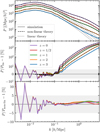 |
Fig. 1 Nonlinear power spectrum at various redshifts compared to linear theory from CLASS (Lesgourgues 2011). The use of the forwardscaling method in the N-body gauge (Fidler et al. 2019) allows the N-body simulation to agree with linear theory at all redshifts including the effects from weak field general relativity, radiation, and massive neutrinos. The narrow ±5% band is plotted using a linear scale, making those fluctuations more visible and allowing also for negative values. Fluctuations at low k are statistical and reflect the sample variance of the particular realisation. At high k the enhanced power is due to nonlinear growth of structure not captured by the linear theory. This nonlinear contribution also includes the slight −2% dip at k ≈ 10−1 h Mpc−1, corresponding precisely to the first BAO peak in the power spectrum. The forward-scaling method used for the Flagship simulation guarantees a match to the linear theory of CLASS at all redshifts, which was not possible to achieve with the traditional back-scaling technique (which only guarantees this at z = 0 in the presence of massive neutrinos and radiation). The bottom panel compares the power spectra to the Euclid Emulator nonlinear power spectrum (Euclid Collaboration: Knabenhans et al. 2021). |
2.2 PKDGRAV3 power spectrum validation
Prior to performing the Flagship simulation, the PKDGRAV3 N -body code was validated against the well-established GADGET3 (Springel et al. 2008), GADGET4 (Springel et al. 2021), ABACUS (Garrison et al. 2021), and RAMSES (Teyssier 2002) codes, which each use very different methods to solve the Poisson equation as well as different methods to integrate the equations of motion. The results of these comparisons are given in Schneider et al. (2016) and more recently in Springel et al. (2021, Fig. 50) and Garrison et al. (2019, Fig. 5). All codes agree at the 1% level up to k = 10 h Mpc−1. Convergence of the power spectrum as a function of the particle mass and simulation box size was also investigated. Conservatively, a particle mass of mp = 109h−1M⊙ is required to ensure 1% convergence of the power spectrum up to k = 10 h Mpc−1 . Simulation boxes larger than 1 h−1 Gpc are sufficient to ensure convergence in the power spectrum (e.g., Klypin & Prada 2018). However, the requirements of a light cone to z = 3, with as little replication of the volume as possible, lead to a box of 3600 h−1Mpc on a side. This simulated box contained 4 trillion dark-matter particles, which yields the mass resolution desired and also corresponds to the limiting number allowed by the Piz Daint supercomputer given PKDGRAV3’s memory requirements (which are about 64 bytes/particle, including the tree structure and all buffers for analysis and management of the Input/Output).
In Fig. 1, we compare the power spectrum measured from the Euclid Flagship N-body dark matter simulation to linear theory computed by CLASS (Lesgourgues 2011) and to the Euclid Emulator nonlinear power spectrum (Euclid Collaboration: Knabenhans et al. 2021). Comparison to the BACCO emulator (Angulo et al. 2021) shows a very similar level of agreement. The ‘spikes’ at lower k are due to the cosmic variance present in the realisation of the Euclid Flagship N-body simulation. When comparing to other models of the nonlinear power spectrum, such as Halofit (Takahashi et al. 2012) and HMCode2020 (Mead et al. 2021), the comparison is not quite as good, with deviations over redshift at k > 0.1 h Mpc−1 extending to ±5%, and notably, these models do not accurately capture the nonlinear form of the baryonic wiggles at k approximately 0.1–0.4 h Mpc−1.
2.3 Dark matter clustering
Galaxy clustering is one of the main probes of the Euclid mission. In order to validate this probe in the galaxy mock, we first study whether the clustering of the dark matter distribution in the lightcone behaves according to theoretical expectations. Figure 2 shows the angular power spectrum of dark matter in thin redshift shells (in the HEALPix tessellation, see Sect. 3 for details), across the full depth of the Flagship N-body lightcone, i.e., 0.5 < z < 3. Measurements in the simulation make use of the PolSpice code (see Szapudi et al. 2001; Chon et al. 2004; Fosalba & Szapudi 2004)4 which corrects for the effect of angular masks in our finite-sky analysis.
Results show that measurements in the simulation agree with linear theory expectations on large scales (low multipoles) and nonlinear theory (Takahashi et al. 2012) down to very small scales (high multipoles, ℓ ~ 104), within sample variance errors (see dotted envelopes in lower panels for each redshift bin). We note that particle shot-noise is negligible (<1% for all multipoles) given the high particle density, around 90 particles/(h−1Mpc)3, in the lightcone. The agreement between Flagship measurements and the Euclid Emulator2 (EE2) predictions is expected to be at a very similar level of agreement, as discussed in Euclid Collaboration: Knabenhans et al. (2021, see in particular their Figure 13) where they show that the EE2 and halofit agree within 3% up to very small (nonlinear) scales, k < 4 h Mpc−1 , for z < 2.
3 HEALPix lensing mass maps
Following the approach presented in Fosalba et al. (2008) and Fosalba et al. (2015), we construct a lightcone simulation by replicating the simulation box (and translating it) around the observer. Given the large box-size used for the Flagship simulation, Lbox = 3600 h−1Mpc, this approach allows us to build all-sky lensing outputs without repetition up to z ~ 2.0 and with one replication up to our maximum redshift, zmax = 3. Then, we decompose the dark matter lightcone into a set of all-sky concentric spherical shells of given width, ∆r, around the observer, what we call the ‘onion universe’. Each dark matter ‘onion shell’ is then projected onto a 2D pixelised map using the HEALPix tessellation (Górski et al. 2005). For the lensing maps presented in this paper we have chosen a shell width of ∆r ≈ 95.22 megayears in lookback time, up to z = 10 (and finer at higher redshifts), and an angular resolution of  , for the HEALPix map resolution Nside = 8192 that we use.
By combining the dark matter ‘onion shells’ that make up the lightcone, we can easily derive lensing observables, as explained in Fosalba et al. (2008). This approach, based on approximating the observables by a discrete sum of 2D dark-matter density maps multiplied by the appropriate lensing weights, agrees with the much more complex and CPU time consuming ray-tracing technique in the Born approximation limit, i.e., in the limit where lensing deflections are calculated using unperturbed light paths (see e.g, Hilbert et al. 2020).
Following this technique we are able to produce all-sky maps of the convergence field (which is simply related to the lensing potential in harmonic space), as well as maps for other lensing fields obtained from covariant derivatives of the lensing potential, such as the deflection angle, shear, flexion, etc. Figure 3 shows the all-sky map of the convergence field, κ, for the Flagship simulation, for sources at zs = 1, with a pixel resolution of 0.′43. The colour scale shown spans over the range −σ < κ < 3σ, where σ is the root mean square (rms) fluctuation of the full-sky convergence map.
The angular power spectrum of the convergence field in the Born approximation reads (for a flat LCDM cosmology),
 (1)
(1)
where ℓ is the multipole order, H0 = 100 h km s−1 Mpc−1 is the Hubble constant, c is the speed of light, and rs is the comoving distance to the lensing sources (we assume all sources are located at the same redshift in this approximation) where P(ℓ/r, r) is the 3D density power spectrum in the simulation at a given comoving distance r from the observer.
In this approach, we can take the spherical transform of the lensing potential all-sky map to obtain the corresponding maps for the other weak-lensing observables through simple relations in harmonic space (see Hu 2000). In particular, the convergence field, κ, is related to the lensing potential, ф, through the 2D equivalent to the usual (3D) Poisson equation, which in spherical harmonic decomposition reads
 (2)
(2)
One can thus use this expression to derive the lensing potential at each source plane (or 2D lightcone map), and obtain other lensing observables, such as deflection and shear, through their relation to the lensing potential in harmonic space (see Fosalba et al. 2015, for details). As a basic validation of the mass maps, Fig. 4 shows the measurement of the convergence angular power spectrum in the simulation compared with theory predictions, for two different source redshifts across the lightcone. Overall there is good agreement between the mass map clustering compared to theory in the full range of scales (multipoles) shown, given the sample variance errors (see figure caption for details).
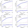 |
Fig. 2 Angular power spectrum of the dark matter field in the lightcone across different redshifts. Plots show the clustering in the following z-bins: 0.49 < z < 0.51 (top left), 0.99 < z < 1.00 (top right), 2.02 < z < 2.08 (bottom left) and 2.94 < z < 3.06 (bottom right). The clustering in the simulation (symbols) is compared against linear (dashed) and nonlinear (solid) theoretical predictions (Takahashi et al. 2012). Particle shot-noise is also shown for reference (dot-dashed line). Residuals with respect to nonlinear theory are displayed in the lower panels, along with sample variance error envelopes (dotted). |
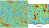 |
Fig. 3 Lensing convergence (colour coded) and shear field (sticks) for sources at zs = 1 over a patch of 50 deg2 (left) and in a zoom-in of the central 1 deg2 area (right). The convergence field colour bar displays values within the range ±3σ, where σ is the rms value of the full-sky map. The stick at the bottom of the zoom-in image shows a reference amplitude for the shear sticks overlaid on that area of the mass map. |
4 Halo catalogue
The dark matter haloes were identified directly on the lightcone particle data using the ROCKSTAR halo finder (Behroozi et al. 2013). ROCKSTAR is a phase space-linking friends-of-friends method that is able to find the hierarchy of substructure from parent dark matter haloes to the smallest subhaloes. ROCKSTAR is also a high-performance parallel halo finder; however, it is not capable of handling such a massive (10 trillion particle) simulation in its standard (public) version. In order to use it for finding haloes in the FS2 particle lightcone data, we had to split the data into computational ‘bricks’ of 375 h−1 Mpc × 375 h−1 Mpc × 625 h−1 Mpc, each with an extended ‘ghost’ region of 5 h−1 Mpc on each side to avoid discontinuities. The full particle lightcone comprises 3448 such computational bricks, each of which could be computed independently on a cloud of (56 core) servers at the University of Zurich. One complication in the processing is that the data in the lightcone is over a variable expansion factor, a, as a function of depth in the lightcone, changing from 1.0 at the centre to 0.25 (z = 3.0) at the edge. This fact must be accounted for when converting the particle momenta to physical peculiar velocities5. ROCKSTAR was written to compute halo catalogues from a set of simulation snapshots, each at a fixed expansion factor, and not from a lightcone and, therefore, needed to be modified to handle particles with radially dependent expansion factor. ROCKSTAR uses these peculiar velocities for both linking (where the linking length in velocity space is adapted from halo to halo) as well as for ‘unbinding’, the process of removing particles from a halo that are deemed not to be gravitationally bound to it (in isolation). Once all haloes within a brick have been found, the parent haloes with centres in the ghost region and subhaloes of such parent haloes are removed from the catalogue so that the individual bricks fit seamlessly together.
The science reach of Euclid depends on how much volume it can sample and how many tracers it can use for cosmological analysis. Its design was optimised to obtain the most stringent constraints on cosmological parameters. For its weak lensing analysis, it reaches magnitude limits of IE ≃ 24.5. The default minimum number of particles for ROCKSTAR to define a halo is set to 20. However, we set the minimum number of particles to define a halo to 10 to be complete at the Euclid weak lensing magnitude limit (see Sect. 4.2.1). As we use such small and poorly resolved haloes, we correct the halo masses of haloes with few particles to avoid incompleteness and discreteness effects in the halo mass function (Sect. 4.2). The final all-sky halo catalogue contains 126 billion main haloes. The galaxy catalogue is generated from the halo catalogue in just one octant of the lightcone that contains 15.8 billion main haloes.
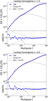 |
Fig. 4 Angular power spectrum of the convergence field at zs = 1 (top) and zs = 3 (bottom). Plots show measurements in the simulation (symbols) compared against linear theory (dashed line) and nonlinear (solid line) fits to simulations (Takahashi et al. 2012). The lower panels show the ratio between the simulation and nonlinear theory. Sample variance error envelopes are displayed as dotted lines. |
4.1 Halo mass function
The ROCKSTAR halo finder produces different estimates of the halo mass. These estimates include: the mass, Mfof, of the particles linked together with a friends-of-friends algorithm of linking length b = 0.2; the mass, Mvir, contained within the virial radius; the sum of the mass, Mbound, of the bound particles within the virial radius; the mass, M200b, of the particles within an overdensity of 200 relative to the background density; and the mass, M200c, of the particles within an overdensity of 200 relative to the critical density. Appendix A provides a comparison of the halo mass function (HMF) for the different halo mass definitions.
Based on the similar behaviour of the HMF with the different mass estimates (except for the friends-of-friends mass definition), we decided to choose the Mbound definition as a default choice to build the galaxy catalogue. As our method of assigning galaxy luminosities is based on AM, the particular choice of mass estimate is not important.
We compare the Flagship Mbound HMF to other HMFs in the literature. As indicative of the behaviour, we present a comparison at low redshift and also as a function of redshift. We use as main reference the Tinker et al. (2008) HMF, hereafter T08, as it has been widely used in the literature for HMF comparison. We also compare it to the HMFs of Despali et al. (2016), D16, and of Comparat et al. (2017), C17. We use the hmf6 (Murray et al. 2013) and COLOSSUS7 (Diemer 2018) packages to compute the HMFs using the reference Flagship cosmological parameters. Figure 5 shows the cumulative HMFs at low redshift, z = 0.1 in the top panel, and the ratio of the Mbound HMF to the other HMFs in the lower panel. We compute the T08, D16 and C17 HMFs for the Mvir mass definition. Our Mbound is almost the same as Mvir for the most massive haloes but differs for the lowest mass haloes due to the unbinding of particles. There is an overall offset of around 3–7% lower abundance in the Flagship Mbound HMF compared to the other predictions for the same cosmology. For halo masses below Mbound = 1011.5 h−1 M⊙, equivalent to ~300 particles, the Mbound HMF starts to be incomplete. The differential HMF shows the same trends as the cumulative HMF. The lightcone has little volume at z = 0.1 and therefore the HMF is very noisy above Mbound = 1013.5 h−1 M⊙.
Figure 6 shows the ratio of the cumulative Mbound HMF to the T08 Mvir HMF at several redshifts spanning the redshift range of the simulation lightcone. While the slopes of the HMFs in the mass range 1011.5 h−1 M⊙ ≲ Mbound ≲ 1013.5 h−1 M⊙ are similar at low redshift, z ≲ 1, at higher redshift, the slope of the Mbound HMF progressively gets shallower than the T08 Mvir HMF. The ratio of the abundance at a given Mbound halo mass compared to T08 abundance at the same halo mass also increases with redshift. Part of the difference may be due to the different power spectrum transfer function used in the Flagship run compared to the input we have given to the hmf code to compute the T08 HMF, generated with CAMB (Lewis et al. 2000) for the same cosmology8. We have performed the same comparison to the D16 and C17 HMFs (not shown in the figure) finding qualitatively the same result. A detailed investigation of the Flagship HMF is beyond the scope of this paper. Our tests suggests that the main cause for the difference is the way haloes are defined and how their masses are computed. In any case, the photometric quantities we compute for the mock galaxies depend on an abundance-matching technique and therefore are not affected by small changes in the HMF. The observed luminosity function is recovered for the galaxies by construction in the AM technique despite any mismatch or incompleteness observed in the mass function of the dark matter haloes.
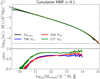 |
Fig. 5 Cumulative Mbound HMF of the Flagship haloes compared to the T08, D16 and C17 halo mass functions at redshift z = 0.1. In the top panel we show the cumulative HMFs (colours indicated in the legend). The lower panel shows the ratio of the cumulative Mbound HMF to the other cumulative HMFs. The dotted line serves as a reference point where the cumulative HMFs are the same. Values of Mbound > 1014 h−1 M⊙ are omitted, since shot noise is dominant due to the small volume available at z = 0.1 in the lightcone. |
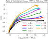 |
Fig. 6 Ratio of the cumulative Mbound HMF to the T08 Mvir HMF at several redshifts indicated in the figure legend. The ratio between the two varies from 7% at low redshift up to 25% at high redshift. The slope of the Flagship cumulative Mbound HMF is shallower than the one of the T08 Mvir HMF at high redshift. The HMFs are shown up to the mass values where they approximately start to be shot-noise dominated. |
4.2 Mass corrections
As we will see later, we assign galaxy luminosities to central galaxies using a halo mass-luminosity relation derived from abundance matching between the cumulative HMF and the cumulative galaxy luminosity function. We push the detection of dark matter haloes to the very low limit of ten particles, making the effects of discreteness very noticeable at the low-mass end of the HMF. Furthermore, as mentioned above, below halo masses of log10[M/(h−1 M⊙)] ≲ 11.5 our HMF starts to be incomplete. In order to produce galaxy luminosities that are not discrete and incomplete, we need to correct the HMF for these two effects.
4.2.1 Incompleteness correction
In order to reach the faint absolute magnitudes that Euclid observes, we need to detect haloes down to the corresponding low masses. For a Euclid magnitude limit of IE = 24.5, we need to reach absolute magnitudes around  log10 h ≃ −13.0 to be complete at redshifts z ≳ 0.1. To reach this absolute magnitude limit, we need to reach a mass limit of M ≃ 2 × 10¹⁰h−1M⊙. Given the resolution of the simulation, this mass corresponds to 20 particles. As we rescale the halo masses to account for the HMF incompleteness, we need to push down to haloes identified with at least 10 particles. With the rejection of unbound particles, the Mbound halo definition can have even fewer particles contributing to the halo mass. At this particle mass threshold, the halo catalogue is not complete. Nevertheless, as the two- point correlation of haloes is approximately independent of mass at low masses, the two-point correlation properties of all haloes detected will not differ from the one it would have had if the catalogue had been complete. That way, we can reassign the halo masses with abundance matching and assume that we are complete to the halo abundance given by the lowest number of particles and that the two-point clustering, which we use to calibrate the galaxy mock, will not change.
We correct for incompleteness by reassigning the halo masses in the following way. We assume that the slope of the cumulative HMF at low masses is the same as the T08 cumulative HMF. Given that the Flagship halo abundance for the Mbound definition is somewhat lower than the T08, we adjust the abundance at a mass log10[M/(h−1 M⊙)] = 11.5, which corresponds to approximately 300 particles per halo. Above this mass threshold, there seems to be no incompleteness due to the low number of particles (see Fig. 5). We reassign the halo masses below this threshold to have the same abundance that a fiducial HMF constructed with the same faint-end slope of the T08 cumulative HMF and normalised to the Flagship cumulative HMF at log10[M/(h−1 M⊙)] = 11.5. The process is captured in Fig. 7 where the original cumulative HMF at redshift z ~ 0.1 is shown in blue, the T08 HMF is shown in black, and the resulting cumulative halo mass after the abundance-matching procedure is shown in red. The new cumulative HMF has the same faint-end slope as the T08 HMF and the normalisation of the original HMF by construction. In fact, there is a slight mismatch at the low- mass end in the corrected cumulative HMF (red line) compared to the rescaled T08 HMF (black line) due to an error in our fitting procedure. This mismatch does not have any significant influence in our resulting catalogue because our abundance-matching procedure absorbs this mismatch.
While this procedure is conceptually simple, implementing it directly into the mock generation is too slow, as one needs to compute the observed cumulative HMF and to invert the T08 cumulative HMF for each galaxy. We therefore developed a faster way of implementing this correction. First, we compute the relation between the original Mbound halo mass and the abundance-matched halo mass. In order to be able to compute this correction efficiently, we fit this relation with five parameters at all redshifts in intervals of 0.1 in redshift. We then fit each parameter as a function of redshift. We also fit the offsets of the cumulative HMF to the T08 values at log10 [M/(h−1 M⊙)] = 11.5.
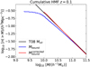 |
Fig. 7 Cumulative HMF at redshift z ~ 0.1 for the Mbound definition (blue), the T08 Mvir HMF (black), and the one resulting from the mass reassignment procedure (red) that corrects for incompleteness and discreteness effects. |
4.2.2 Discreteness correction
We correct for discreteness by assuming that the cumulative HMF is well defined at the mass values corresponding to a given integer number of particles. We proceed as follows. In a given volume V for each number of particles pi, we have Ni haloes with those pi particles corresponding to a halo mass Mi = pi mp. The cumulative abundance for this halo mass is  , that is, the number of haloes with mass larger or equal than Mi divided by the volume. For all haloes with pi particles, we want to reassign their masses to distribute them according to a power-law distribution in abundance between masses Mi and Mi +1. For low masses, it is a good approximation to assume that the cumulative HMF behaves as a power law,
 (3)
(3)
in a small range of masses. For each halo with pi particles and mass Mi, we draw a random number u uniformly distributed in the range [0,1] and use this number to obtain a halo mass M from the normalised cumulative halo mass distribution between Mi and Mi+1,
 (4)
(4)
assigning a halo mass
![Mathematical equation: $M = {\left[ {u\left( {M_i^\beta - M_{i + 1}^\beta } \right) + M_{i + 1}^\beta } \right]^{{1 \over \beta }}}.$](/articles/aa/full_html/2025/05/aa50853-24/aa50853-24-eq9.png) (5)
(5)
So, in order to make the halo mass distribution continuous, we only need to know the slope β of the cumulative HMF as a function of mass and also as a function of redshift (as it evolves). We produce functional fits to the value of the slope to be able to have the slope at any value of the mass and redshift faster than by computing the cumulative HMF in every step.
4.3 Halo clustering
Figure 8 shows the angular clustering of haloes in harmonic space in the lightcone, for the redshift range z = 0.5–1.5, and for two mass bins (1013h−1M⊙ > Mh > 1012h−1M⊙, and 1012h−1M⊙ > Mh > 1011 h−1M⊙, top and bottom rows, respectively). The theory predictions correspond to the dark matter clustering globally rescaled with an estimate of the linear halo bias, fitted to match the measured clustering on the lowest multipoles. We also show the clustering corrected with a simple model for the shot-noise. The resulting (corrected) clustering is in good agreement with linear theory expectations at low multipoles, i.e, ℓ < 200 at z = 0.5, and ℓ < 500 at z = 1.5, within sample variance errors (see lower panels). These limiting multipoles are only approximate given that the scales beyond which linear matter growth and the linear halo bias model break down depend both on redshift and halo mass. We also note we have assumed that haloes are Poisson distributed which is not strictly the case (Ginzburg et al. 2017). However a proper correction of the shot-noise for halo clustering is beyond the scope of this paper.
5 From haloes to galaxies
Galaxies were generated in the Flagship simulation using a prescription that includes HOD and AM techniques and observed relations between galaxy properties. The prescription follows the methodology used in populating the MICE Grand Challenge simulation with galaxies (Carretero et al. 2015, C15 hereafter). The starting point is the Flagship halo catalogue described above. We use the SciPIC algorithm, described in Appendix B, to compute the galaxy properties. We run the pipeline at the Spanish Euclid Science Data Center. In the following subsections, we describe the different steps of the galaxy catalogue production.
5.1 Galaxy luminosities
Following the HOD philosophy, haloes are populated with central and satellite galaxies. Our prescription starts with a hybrid HOD and AM method, that computes the number of satellites in each halo and assigns the galaxy luminosities. Galaxy clustering measurements are used to determine the parameters and the relations implemented.
The method has the following steps. First, it assumes that each halo is composed of one central galaxy and some satellites. We use a simple HOD in which the mean number of satellites (the satellite occupation) depends only on the halo mass as a power law. For all haloes with masses larger than the minimum halo mass (Mh ≥ Mmin), the number of central galaxies and the mean number of satellite galaxies are given by
 (6)
(6)
We assign the number of satellite galaxies in each halo drawing a realisation of a Poisson distribution with mean 〈Nsat〉. We parameterise M1 as a multiplicative factor, f times Mmin:
 (7)
(7)
In MICE, we calibrated the factor f as a function of halo mass to match the SDSS two-dimensional projected clustering constraints of Zehavi et al. (2011) at low redshift. In the Flagship simulation, we adopt a constant value for the multiplicative factor in (7) and fix it to f = 15, which is approximately the mean value we used in MICE (Carretero et al. 2015). We further choose the multiplicative factor not to depend on redshift given the weak constraints on galaxy clustering at high redshift. We also set the exponent in Eq. (6) to a fixed value, α = 1, with no redshift dependence either. We will show in Sect. 6 that our galaxy mock gives results that are in good agreement with a large set of observational data.
We then use AM to assign the galaxy luminosities. In order to obtain a relation between the halo mass and the central galaxy luminosity, we first calculate the cumulative number density of galaxies (central and satellites), ngal , as a function of the halo mass9. We compute this function by integrating the CHMF, taking into account the HOD assignment,
![Mathematical equation: ${n_{{\rm{gal}}}}\left( { > {M_{\min }}} \right) = \int_{{M_{\min }}}^\infty n \left( {{M^\prime }} \right)\left[ {1 + {{\left( {{{{M^\prime }} \over {f\,{M_{\min }}}}} \right)}^\alpha }} \right]{\rm{d}}{M^\prime },$](/articles/aa/full_html/2025/05/aa50853-24/aa50853-24-eq12.png) (8)
(8)
where we have used Eqs. (6) and (7) to compute the number of galaxies per halo at the mass threshold, Mmin. Both ngal and n are densities, that is, number of galaxies per unit volume. We refer to this function defined in Eq. (8) as the cumulative galaxy number density function (CGNDF).
The adopted galaxy luminosity function (LF) for the AM is a variation of the function given by Dahlen et al. (2005), which is based on multi-band data taken in the Great Observatories Origins Deep Survey (GOODS; Giavalisco et al. 2004). The GOODS LF is parameterised in several optical and near-infrared bands up to redshift z = 2. We extrapolate it to higher redshifts, z = 3, and fainter luminosities, and transform it to our reference band. The total luminosity function is the sum of the LFs of three populations, each with its own evolution. As most of our calibration is inherited from the MICE catalogue which was performed at low redshift using SDSS data, and in particular the New York University Value Added Galaxy Catalogue (NYU-VAGC; Blanton et al. 2005b), we choose as our reference filter the SDSS r01 band10, which is the SDSS r filter redshifted to z = 0.1 (Blanton et al. 2003). Figure 9 shows the cumulative LF function in the r01 band for several redshifts.
Several studies have shown that when generating a galaxy mock catalogue with AM using the observed cumulative LF, the resulting galaxy clustering amplitude for the most luminous galaxies is higher than observed. The clustering amplitude for these luminous galaxies can be lowered if scatter is applied in the luminosity assignment (e.g., Tasitsiomi et al. 2004; More et al. 2009; Behroozi et al. 2010; Reddick et al. 2013; Carretero et al. 2015). Given that the highest luminosity range is dominated by an exponential decay, the introduced scatter results in assigning higher central galaxy luminosities to haloes of lower masses, thus reducing the amplitude of the clustering at the high luminosity range. Nevertheless, at lower luminosities where the LF is mainly dominated by a power law, the inclusion of this scatter has no effect in the overall shape of this function. Besides obtaining a more realistic clustering for the most luminous galaxies, introducing this scatter also reflects the fact that galaxy formation is a stochastic process. Taking this into account, we apply a scatter to the galaxy luminosities resulting from the AM step. We define an unscattered LF, Φunscat(L), that when convolved with a Gaussian scatter in the logarithm of the luminosity (function G in Eq. (9)) gives the observed LF, Φobs(L),
 (9)
(9)
where the Gaussian function G has a mean of zero and a standard deviation of ∆ log10[L/(h−2L⊙)]. To obtain the unscattered LF, we need to solve for Φunscat(L) in the convolution equation (9). Instead, to gain computing efficiency, we approximate the effect of the convolution with an exponential decay factor:
![Mathematical equation: $\eqalign{ & {\Phi _{{\rm{unscat }}}}\left( {L,z,\Delta {{\log }_{10}}L} \right) \cr & \quad = {\Phi _{{\rm{obs }}}}(L,z)\exp \left[ { - {{\left( {{L \over {{L_{{\rm{sct}}}}\left( {z,\Delta {{\log }_{10}}L} \right)}}} \right)}^{{\beta _{{\rm{sct}}}}\left( {z,\Delta {{\log }_{10}}L} \right)}}} \right], \cr}$](/articles/aa/full_html/2025/05/aa50853-24/aa50853-24-eq14.png) (10)
(10)
where we fit the parameters Lsct, and βsct as a function of redshift, z, and the value of the scatter, ∆ log10[L/(h−2L⊙)]. We compute the cumulative unscattered LF as
 (11)
(11)
where we have omitted the dependence on redshift and the luminosity scatter. We can establish a relation between halo mass and luminosity by applying AM between the cumulative number density of galaxies function (Eq. (8)) and the cumulative unscattered LF (Eq. (11)):
![Mathematical equation: ${n_{{\rm{gal }}}}\left( { > {M_{{\rm{halo }}}},z} \right) = {n_{{\rm{gal }}}}\left( { > L,z,\Delta {{\log }_{10}}\left[ {L/\left( {{h^{ - 2}}{L_ \odot }} \right)} \right]} \right).$](/articles/aa/full_html/2025/05/aa50853-24/aa50853-24-eq16.png) (12)
(12)
Equation (12) establishes the relation between halo mass and galaxy luminosity, which is commonly referred to as the galaxy-halo connection. Although, normally this connection is expressed in term of the galaxy stellar mass instead of galaxy luminosity in the stellar–halo mass relation (SHMR). There have been many studies in recent years trying to understand how galaxies form in dark matter haloes and how this relation is established. Its exact form depends on the processes of star formation and feedback. Wechsler & Tinker (2018) provides a review of the galaxy-halo connection including many references to previous work.
Figure 10 shows the resulting AM relations for a few redshift values from Eq. (12) for our assumed value of ∆ log10[L/(h−2 L⊙)] = 0.12. The relation is fitted as a double power law (e.g., Yang et al. 2003; Moster et al. 2010) with parameters fitted as a function of halo mass and redshift. The luminosities of the central galaxies are assigned from their halo mass and their redshift using the relation coming from Eq. (12) and shown in Fig. 10 for a few redshift values. We then add a random realisation of the scatter in the logarithm of the luminosity to its value assuming a Gaussian distribution. We take the standard deviation of this distribution to be ∆ log10[L/(h−2 L⊙)] = 0.12, which is similar to the value applied in other studies (e.g., Reddick et al. 2013) and produces a consistent clustering signal in our catalogue at high luminosities and at low redshift.
In order to assign luminosities to the satellites, we first compute the global LF for these galaxies by subtracting the LF for the centrals from the total LF used to compute the AM. Figure 11 provides a visual representation of this step. It shows the model LF used to compute the AM relation between mass and luminosity and the measured LF in the Flagship catalogue in a thin redshift slice centred at z = 0.5 for all the galaxies and for centrals and satellites only. Once we have the global LF for the satellites (blue line in Fig. 11), we assume that it is the result of the sum of the individual LFs of satellites within each halo for all haloes. We model the cumulative LF of the satellites within each halo using a modified four-parameter Schechter function of the form
![Mathematical equation: $N_{{\rm{sat}}}^{{\rm{halo}}}( > L) = A{\left( {{L \over {{L_*}\left( {{L_{{\rm{cen}}}}} \right)}}} \right)^\alpha }\exp \left[ { - {{\left( {{L \over {{L_*}\left( {{L_{{\rm{cen}}}}} \right)}}} \right)}^\beta }} \right],$](/articles/aa/full_html/2025/05/aa50853-24/aa50853-24-eq17.png) (13)
(13)
where A is the normalisation factor that ensures that the halo contains the number of satellites predicted by the realisation of the HOD with luminosities higher than the minimum luminosity assigned for that halo, Lmin, α is the faint slope that we fix to α = −0.5, and β is a parameter that controls the steepness of the bright-end exponential cut-off. Furthermore, L* is the characteristic luminosity that depends linearly on the luminosity of the central galaxy, L* = a Lcen + b. Taking into account this model for each halo, we fit the three parameters, a, b, and β, to make the sum of the satellite LF of all the haloes match the global LF. We obtain the values a = 10−0.5, b = 0 and β = 1.5 from this process. Finally, we assign the luminosities for the satellites in each halo by randomly drawing the luminosities following Eq. (13). Since we generate luminosities drawing realisations from functional forms that are fitted to all the redshift and luminosity ranges of the simulation, there are slight mismatches between the LF at particular redshifts for the generated and model LFs, as can be seen in the green (all generated galaxies) and black (model) curves of Fig. 11.
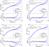 |
Fig. 8 Angular power spectra of the dark matter haloes in the lightcone at redshifts z = 0.5 and 1.5. The top panels show the clustering for haloes of mass 1013h−1M⊙ > Mh > 1012h−1M⊙, whereas the bottom panels display the corresponding results for 1012h−1M⊙ > Mh > 1011 h−1M⊙. The lower panels show the ratios with respect to nonlinear theory, with dotted lines displaying the envelope for sample variance errors. |
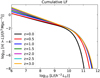 |
Fig. 9 Cumulative luminosity function of the galaxy population in the r01 band at different redshifts used in our abundance-matching procedure. This LF is an adaptation and extrapolation to higher redshifts and fainter luminosities of the GOODS LF given by Dahlen et al. (2005). The LFs at the high luminosity end are hardly distinguishable at z > 1. |
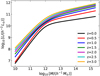 |
Fig. 10 Relation between halo mass and luminosity at various redshifts resulting from abundance matching the cumulative galaxy function and the cumulative unscattered luminosity function following Eq. (12). |
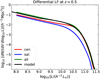 |
Fig. 11 Differential luminosity function for central and satellite galaxies, and all galaxies at redshift z = 0.5 in the Flagship catalogue. We also show the model LF as in Fig. 9 but in its differential form. |
5.2 Galaxy colours and positions
Before allocating positions and velocities to the galaxies, we assign them a (g01 − r01)HOD11 colour, defined as the colour computed using the g and r SDSS filters redshifted to z = 0.1 (Blanton et al. 2003). This colour is used together with the luminosity and redshift to assign the spectral energy distribution to the galaxies (see Sect. 5.4). We define three colour populations and assign individual colours to galaxies depending on which population they belong to. The abundance of these colour populations in each halo is defined by the HOD prescription. We follow the same procedure as C15 to assign the (g01 − r01)HOD colour that depends on the galaxy type. We have extended the C15 fits to fainter luminosities as the Flagship catalogue contains haloes of lower mass and thus reaches fainter luminosities. A full description of the method is given in C15. We summarise it here, noting the extensions and improvements made.
We start from the colour-magnitude diagram (CMD) using the low-redshift NYU-VAGC SDSS galaxy catalogue (Blanton et al. 2005a), which we show in Fig. 12. We fit the g01 − r01 colour distribution as a function of luminosity in this colourmagnitude diagram to three galaxy populations: blue, green, and red. Similarly to what was done in Baldry et al. (2004), Skibba & Sheth (2009), and Carretero et al. (2015), we assume that the three populations are characterised by Gaussian distributions. In fact, we detect another population at bright absolute magnitudes, Mr01 − 5 log10 h ≲ −22), which is redder than the main Gaussian-distributed red population. Since the green population has no galaxies brighter than Mr01 − 5 log10 h ~ −22, the extra red and green populations do not overlap in the CMD. Therefore, for computational convenience, we absorb this extra red population within the green population. We fit the means and standard deviations of the Gaussian distributions of each population as a function of luminosity. Figure 12 includes these fits to the means and standard deviations as solid and dotted lines, respectively, in the colour-magnitude diagram. The red, green, and blue lines correspond to the red, green, and blue populations, respectively. As an example of these fits, Fig. 13 presents these three colour distributions at the absolute magnitude Mr01 − 5 log10 h ≲ −22.0. The mean and standard deviations of the three populations are fit by global functions that depend on the absolute magnitude. These are the functions shown in Fig. 12 and not the individual values at the absolute magnitude bins used to define the functions.
We adopt the procedure of Skibba & Sheth (2009) and followed in C15 to compute the (g01 − r01)HOD colour based on the galaxy type (central or satellite). We also differentiate the galaxies into three colour types defined by the Gaussian fits of the CMD. We assign the parameter color_kind to each galaxy in the catalogue to indicate to which colour population it belongs to: red, green, or blue. We define a function to determine the fraction of satellites that belong to the red population as a function of luminosity and another one for the green population. The HOD and the colour-magnitude diagram then determine the fraction of satellites that belong to the blue population and the fraction of centrals that belong to the three populations (see Eqs. (37)–(43) in C15). These functions were optimised in MICE to reproduce the clustering as a function of colour and luminosity of the SDSS sample (Zehavi et al. 2011). For Flagship we modified these functions slightly and extended them to lower luminosities. However, we did not run a proper minimisation exercise, in part due to the flexibility in the functional form that we have allowed. Figure 14 shows these functions as implemented in the Flagship catalogue. All the brightest galaxies are centrals. Then, there is a transition around the LF characteristic luminosity, L⋆, where the fraction diminishes to become approximately constant around 50% for lower luminosities. The overall fraction of red, green, and blue galaxies is constrained by the CMD, with many more red galaxies at bright luminosities and blue galaxies dominating the population at faint luminosities. At all luminosities, there is a higher fraction of red galaxies that are satellites than centrals, and the other way around for blue galaxies. The fraction of green galaxies is always low compared to the red and blue ones. As mentioned before, galaxies brighter than absolute magnitudes Mr01 − 5 log10 h ≃ −21.5, which are tagged as green are indeed redder than the main red population. The fraction of green satellites is larger than that of green centrals for the true green population at low luminosities, but the trend is reversed at bright luminosities, where all this extra population of the reddest galaxies (tagged as green) are centrals.
Figure 15 displays the fraction of color_kind values as a function of luminosity at four redshifts, splitting between centrals and satellites. There are no more local minima or maxima in the fractions vs. luminosity as were seen in Fig. 14, because of the split in redshift bins. The Flagship galaxies show the following trends: 1) luminous galaxies are redder, consistent with what is observed at low redshifts (Sandage & Visvanathan 1978); 2) satellites are more likely to be red than centrals of the same luminosity, as observed at low redshifts (van den Bosch et al. 2008); 3) centrals and satellites (in particular low-luminosity ones) are more likely to be blue at higher redshifts, in conformity with the Butcher–Oemler effect (Butcher & Oemler 1978) that galaxies in higher-redshift clusters contain a higher fraction of spiral morphologies (hence bluer colours).
We place the central galaxies at the centre of their haloes. Satellite galaxies are located following a triaxial Navarro, Frenk, and White (NFW; Navarro et al. 1997) profile. We use the virial radius, the concentration parameter, and the vectors of the ellipsoid semi-axes to compute the satellite positions. We obtain the concentration parameter of the haloes using the virial radius and the scale radius from the ROCKSTAR catalogue12 for haloes with masses log10[Mhalo/(h−1 M⊙)] > 11.0, where there are enough particles per halo as to reliably determine the concentration. For this mass range, the concentration parameter agrees with a mass dependence that matches that given by Diemer & Joyce (2019) as computed with the COLOSSUS code. Below this mass threshold, we use the relation from Diemer & Joyce (2019) to obtain the mean concentration for a given halo mass and redshift. We have computed the ratio of the standard deviation to the mean of the distribution of concentration parameters as a function of halo mass and redshift. This ratio is approximately constant with a value of 1/3. We therefore assign the concentration parameter for the haloes below the mass threshold Mhalo = 1011 h−1 M⊙, drawing a realisation of a Gaussian distribution with the mean coming from the relation of Diemer & Joyce (2019) and a standard deviation that is one-third of the value of the concentration mean. Figure 16 shows with red dots the mean of the concentration parameter as a function of halo mass at three different redshifts before correcting the values at low halo mass. The red lines indicate the standard deviation of the concentration parameters. The black line shows the Diemer & Joyce (2019) relation. The recomputed mean concentration values at low halo mass coincide with the black line.
The fraction of satellite galaxies that belong to poor-resolved haloes (e.g., Mhalo < 1011 h−1 M⊙) is very small in the final catalogue and, thus, not very important. For an HE < 26 selected sample that fraction is around 1%. For weak lensing and galaxy clustering Euclid-like samples, it is below 0.1%.
The other ingredient for assigning positions to the satellites within their haloes is the triaxial shape of the haloes. ROCKSTAR outputs the position vectors of two of the ellipsoid semi-axes and the axis ratios. We compute the third position vector as the cross product of the other two. We take the virial radius in the semi-major axis direction as the virial radius provided by the catalogue and in the other directions we multiply the virial radius by the corresponding axis ratios. We assign the position of satellite galaxies within haloes following the procedure of Robotham & Howlett (2018)13, which we modify to compute random positions in a triaxial NFW keeping the appropriate density profile, axis ratio values, and ellipsoid orientation. We compute the positions in each halo coordinate system given by the position vectors of their semi-axes and then transform them to comoving coordinates taking into account the orientation of the ellipsoid with respect to the observer’s lightcone.
We implement colour segregation in the satellite galaxy distribution assuming a different concentration parameter for each of the color_kind samples (e.g., McDonough & Brainerd 2022). Red galaxies have the same concentrations of the dark matter in the haloes. Blue galaxies have a concentration one fourth of the concentration of the red galaxies (following Collister & Lahav 2005), while green galaxies have a concentration half of that of the red galaxies. Following C15 who placed galaxies beyond the virial radius to adjust the galaxy clustering in the MICE catalogue, we also place satellites beyond the halo virial radius up to three times its value, resulting in approximately 15% of the satellite galaxies being outside the virial radius of their haloes. As discussed in Sect. 6.4, this is an oversight, given the different ways that haloes and their boundaries are defined in the Flagship simulation in comparison to MICE, resulting in overpopulating with galaxies the regions outside the virial radius.
Figure 17 shows the 3D number density profile of halo galaxies in a slice of redshift and halo mass. We restrict the plot to 188 haloes in the redshift range, 0.6 < z < 1.0, and in the halo mass range, 14.0 < log10[M/(h−1 M⊙)] < 14.4, containing a total of over 104 member galaxies (with IE < 24.5 and HE < 24) within the virial radius: 6423, 1308, and 2877, Red Sequence, Green Valley, and Blue Cloud galaxies, respectively. One clearly sees the different radial distributions for the Red-Sequence, Green-Valley, and Blue-Cloud galaxies, with the latter having a concentration four times lower than for the Red-Sequence galaxies, as designed and shown in Table 1. The stacked radial distribution for all galaxies (black in Fig. 17) is also well fit by an NFW model, even if it is the composite of three NFW models with very different scale radii. The best-fit concentration for all galaxies is intermediate between the extreme red and blue colour classes. One also sees that the profile follows the NFW model very well out to ≃1.8 rvir, beyond which only a fraction of galaxies are halo members because of the triaxiality of the haloes (Sect. 5.2).
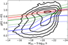 |
Fig. 12 Colour-magnitude diagram of the SDSS NYU-VAGC (Blanton et al. 2005a). The black lines show contours of the same density of galaxies in this space. The red, green, and blue solid lines show the mean of the distributions of the three Gaussian fits to the (g01 − r01) colour distributions as a function of absolute magnitude. The dotted lines show the position of the mean ± the standard deviation of the Gaussian distributions. |
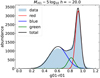 |
Fig. 13 Colour distribution of galaxies in the SDSS NYU-VAGC at absolute magnitude Mr01 − 5 log10 h = −20.0. The light blue histogram represents the data in the catalogue. The red, green, and blue lines are the fits to the three Gaussian populations and the black line the sum of the three. |
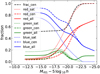 |
Fig. 14 Galaxy fractions as a function of absolute magnitude. The black dashed line represents the fraction of centrals, while the rest of the lines present combinations of galaxy type and galaxy colour type. The line style distinguishes centrals (dashed lines) from satellites (dotted lines) and all galaxies (solid lines). The galaxy colour types are presented with different colours: red, green, and blue. |
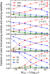 |
Fig. 15 Fraction of galaxies of different types as a function of absolute magnitude for different redshift slices (∆z = ±0.1), split between Red Sequence (‘RS’), Green Valley (‘GV’), and Blue Cloud (‘BC’), and between centrals (‘cens’) and satellites (‘sats’). The abscissae have been slightly shifted for clarity. |
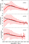 |
Fig. 16 Concentration index as a function of halo mass at the redshifts marked in each panel. The red dots correspond to the means of the distributions at each halo mass bin and are linked with a red line. The vertical red lines show the standard deviations of the distributions. The black line shows the Diemer & Joyce (2019) functional form values. |
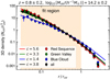 |
Fig. 17 3D galaxy number density profiles of stacks of Flagship haloes, after removing all haloes lying closer than 3 rvir from the edges of the region. The maximum likelihood concentration parameters (virial radius over NFW scale radius), obtained by fitting an NFW model to the distribution of radial distances r (restricted to the shaded region), are shown in the legend. |
Assumptions for deriving velocity dispersions.
5.3 Galaxy velocities
Once the galaxy positions are determined, we compute their velocities within the halo. We also use the parameter color_kind to produce line-of-sight velocity dispersion profiles modulated by the type of galaxy.
Central galaxies are assumed to be at rest at the centre of the halo, so their velocity is the same as the centre of mass of the halo. The satellite galaxy velocities are built by solving the spherical, stationary, Jeans equation of local dynamical equilibrium,
 (14)
(14)
for given radial profiles of mass M(r), number density ρ(r), and velocity anisotropy  , with σθ and σr being the velocity dispersion in the tangential and radial directions, respectively. The velocity anisotropy is assumed to follow the Tiret et al. (2007) model:
 (15)
(15)
which is a reasonably good approximation to what is seen in ΛCDM haloes. Using the parameters found for massive clusters at z = 0.05 by Mamon et al. (2019), assuming that ellipticals, S0s and spirals respectively trace red sequence, green valley, and blue cloud galaxies as defined by the color_kind parameter, leads to the parameters given in Table 1.
We proceed as follows:
Pre-compute the radial velocity dispersions in virial units, σr (r)/υvir on a two-dimensional grid of geometrically spaced r/rvir and concentrations, where the σr are obtained by solving (following Eq. (C.1)) the Jeans equation in Eq. (14) using the assumptions of Table 1;
pre-fit three two-dimensional 5th-order polynomial approximations (one per color_kind) for log10 (σr /υvir) in terms of log10(r/rvir) and log10 cdark;
determine the full set of radial velocity dispersions using these polynomial approximations (extrapolating beyond the fit limits with the constant value at each limit);
determine the tangential components of the velocity dispersions, using
 , where the first equality comes from the assumption of spherical symmetry (σθ and σϕ are the azimuthal and latitudinal components respectively of the tangential velocity component);
derive the three velocity components in spherical coordinates, assuming locally Gaussian velocity distribution functions;
convert these physical velocities in the halo frame to peculiar velocities, by subtracting the Hubble flow, H(z) r, from the radial velocity component;
convert these peculiar halo-frame velocities in spherical coordinates to Cartesian coordinates;
convert these peculiar halo-frame Cartesian coordinates into the box frame;
derive the line-of-sight velocities VLOS = (R · V)/R (where R and V are the position and velocity vectors measured relative to the observer and R the modulus of the R vector) in the box frame, assuming that the observer is at rest in the box;
-
derive the redshift from the line-of-sight velocities using the relation
 (16)
(16)where zcos is the cosmological (true) redshift, VLOS is the line-of-sight velocity component, and neglecting the peculiar motion of the observer as well as the 2nd-order transverse Doppler term which incorporates the multiplicative Lorentz factor (1 − V−2 /c2)−1/2 (e.g., Tatum 1985).
The details of steps Nos. 1 and 2 are provided in Appendix C. In a forthcoming (already coded) version of Flagship, we inserted after item No. 6 the addition of a radial infall pattern, obtained by fitting a nonlinear function of redshift and log halo mass to the radial motions inside haloes of dissipationless cosmological simulations.
5.4 Spectral energy distributions
As described in Sect. 5.1, we assign a (g01 − r01)HOD colour to each galaxy randomly sampling the colour distributions derived from the CMD for our three color_kind populations. This colour corresponds to the rest-frame colour of a galaxy in the g01 and r01 filters (see Sect. 5.2) or equivalently the g − r colour at redshift z = 0.1.
Next, we want to assign a spectral energy distribution (SED) to each galaxy. We take as a template basis the COSMOS SED library used in Ilbert et al. (2009) that originally comes from the SEDs of Polletta et al. (2007), complemented with templates from Bruzual & Charlot (2003) to expand the range of star-formation histories included. In order to increase the SED coverage, each galaxy SED is computed as a linear combination of two of the templates in the SED basis.
Following Ilbert et al. (2009), our chosen SED library is composed of 31 templates. We add extinction to some of the templates to expand the colour space coverage and better represent observations. We do not apply any extinction to the first ten reddest templates. The next thirteen templates represent spectral distributions of spiral galaxies and are assumed to have the Prévot Small Magellanic Cloud extinction law (Prévot et al. 1984). The last eight bluest templates represent starburst galaxies and have the Calzetti extinction law (Calzetti et al. 2000). We build a sample of 136 templates using the 31 SEDs and the two extinction laws that we sample at six values of the E(B − V) colour excess (or reddening) from 0 to 0.5 in steps of 0.1. Table 2 summarises the original templates used with their order number, the extinction law applied for those templates, the reddening values sampled for each of those templates, and the total number of resulting SEDs that constitute our SED template basis.
For these 136 templates, we compute the g01 − r01 and the COSMOS g − r colours at seven discrete redshift values covering the redshift range of the lightcone simulation, 0 < z < 3, in intervals of ∆ z = 0.5. Figure 18 shows a subset of six of these 136 templates at redshift z = 0.0.
We rank order the templates according to their colour at these redshift values14. We use the g01 − r01 colour at z = 0 and the COSMOS g − r at the rest of the redshift values for the ordering. We compute a relation between the template order number, treated as a real number but sampled at integer values, and the values of the colour at each redshift value. This relation serves to assign an ordered template number for a given colour value. We smooth this relation to make the function monotonic and avoid degenerate values in the relation that would give the same template order number for different values of the colour. We also establish relations between the g01 − r01 and g − r colours at all non-zero redshift steps. To obtain these relations we abundance match the (g01 − r01)HOD colour distribution in the Flagship catalogue to the g − r colour distribution of the COSMOS2020 catalogue (Weaver et al. 2022) at each redshift value considered (see footnote 14). We take all galaxies in a range of ∆z = 0.2 centred at the mean redshift value to build the samples for the abundance matching. The only exception is for the last redshift value, z = 3.0, where we take galaxies in the range 2.8 < z < 3.0 as there are no Flagship galaxies beyond that redshift. We also compute the E(B − V) distributions from the COSMOS2020 catalogue at the same redshift values, in this case in a redshift range of width ∆z = 0.1. Figure 19 shows the normalised distribution of E(B − V) values in the COSMOS2020 catalogue for a sample with a magnitude limit in this catalogue of i < 24.5, equivalent to the 10 σ magnitude limit of the Euclid Wide Survey in the IE filter. The distribution transitions from being dominated by galaxies with no internal extinction at z = 0.1 to peaking at values of E(B − V) ~ 0.2 at redshifts z ≳ 1.
Our procedure to assign an SED to a galaxy consists of the following steps. First, we determine the two redshift values immediately lower, z1 , and larger, z2 , than the redshift of the galaxy from the list in footnote 14, so that z1 < z < z2. We determine two SEDs from our 136 template basis, one at each of these two redshifts, SED (z1) and SED (z2), and compute the final SED of the galaxy as a linear combination of the two templates (Eq. (17)) with weights, w1 and w2 proportional to their redshift difference to the reference redshift as in Eq. (18),
 (17)
(17)
 (18)
(18)
We derive the SED at each of these two redshifts from the (g01 − r01)HOD colour of the galaxy. We obtain the ordered template number from the colour using the relations found previously. At z = 0.1, we use the relation with the (g01 − r01)HOD colour. At higher redshift we first obtain the COSMOS g − r colour from the (g01 − r01)HOD colour using the abundance-matched relations described before and then use this g − r colour to obtain the ordered template number. We take the six closest ordered templates to this ordered template number from our 136 SED template basis and compute the colour difference from the original colour, either (g01 − r01)HOD or g − r, depending on the redshift, and the colour of these six ordered templates. We compute a probability based on this colour difference for each of these six ordered templates, Pcolour . This probability is assumed to be a Gaussian distribution with mean the original colour and standard deviation half the mean value of the colour differences for the six ordered templates. If the standard deviation is lower than 0.015, we set it to this minimum value. We then compute the probability of the template given its E(B − V) value, PE(B−V), using the distributions of E(B − V) values from the COSMOS2020 catalogue obtained before (Fig. 19). We compute the final probability of each ordered template as the product of these two probabilities in colour and colour excess, Pot = Pcolour PE(B−V) . We generate the cumulative distribution of this probability and draw a random number from which we obtain the ordered SED template using the inverse of the cumulative probability distribution. We perform this procedure at the redshifts z1 and z2, and obtain the final SED following Eqs. (17) and (18). In order to clarify the procedure, we provide an example of an SED assignment in Appendix D.
SED template basis.
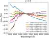 |
Fig. 18 Subset of six SED templates out of the 136 described in the text at redshift z = 0.0. The templates are normalised to have the same flux at a wavelength of 6000 Å. The figure inset indicates the colour-ordered template number (o), the original template number in Ilbert et al. (2009) (t), the E(B − V) reddening value applied to the template (ebv), and the value of the g01 − r01 colour (c). |
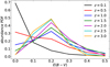 |
Fig. 19 Distribution of E(B − V) values in the COSMOS2020 catalogue for a magnitude range i < 24.5. The distributions are normalised so that the total abundance for all E(B − V) values at each redshift adds up to 1. |
5.5 Galaxy shapes and sizes
Galaxy shapes and sizes are assigned using phenomenological prescriptions similar to those of Miller et al. (2013) with calibration data coming from Hubble Space Telescope (HST) observations. We use two main data sets as calibrators: the Cosmic Assembly Near-Infrared Deep Extragalactic Legacy Survey (CANDELS; Grogin et al. 2011; Koekemoer et al. 2011) reductions of Dimauro et al. (2018) and the Advanced Camera for Surveys15 (ACS) reductions of the GOODS-South field of Niraj Welikala (hereafter referred to as HST_GS, private communication). Our approach is simplistic, since we do not attempt to fit all the galaxy morphological properties while simultaneously keeping the correlations between parameters. Nevertheless, our catalogue is designed to reproduce the one-parameter distributions that we calibrate our data with.
Most galaxies are assumed to have two components: a Sérsic profile (Sérsic 1963) component, which we refer to as bulge, and an exponential disk component. The exception are galaxies fulfilling the following relation:
![Mathematical equation: $\eqalign{ & {(g01 - r01)_{{\rm{HOD }}}} > (0.96 + 0.04z) \cr & \,\,\,\,\,\,\,\,\,\,\,\,\,\,\,\,\,\,\,\,\,\,\,\,\,\,\,\,\,\,\,\,\,\,\,\,\,\,\, - 0.015\left[ {\left( {{M_{r01}} - 5\,\,{{\log }_{10}}h} \right) + 24.0} \right], \cr}$](/articles/aa/full_html/2025/05/aa50853-24/aa50853-24-eq25.png) (19)
(19)
where z is the galaxy redshift and Mr01 − 5 log10 h is the absolute magnitude in the r01 filter. These galaxies are described by a single Sérsic profile component, which we also call bulge. We identify this modelling difference with the parameter dominant_shape in the catalogue which is set to 0 for the one-component (bulge only) profile galaxies and to 1 for the two- component (bulge and disk) galaxies. The selection in Eq. (19) implies that the reddest galaxies at each magnitude are the ones modelled with a one-component (bulge only) profile. The fraction of these galaxies to the total number of galaxies varies as a function of magnitude as shown in Fig. 20, with the fraction getting smaller as magnitudes get fainter. We chose to use a simple magnitude-dependent colour cut to separate the way to model the galaxies. This cut reproduces well the fraction in the CANDELS catalogue of Dimauro et al. (2018) at magnitudes brighter than i < 22, but it is lower at fainter magnitudes. For these fainter galaxies, their smaller sizes and lower signal-to-noise detections make the distinction of two profile components harder. The upward trend seen in CANDELS at i > 23 can probably be attributed to this effect. Taking this into account and as the one- and two-component models are not very different for these small sizes for the Euclid pixel size, we decided not to change this simple selection cut for faint magnitudes. As the catalogue is dominated by faint galaxies, the overall fraction of bulge-only galaxies is approximately 10% of the total galaxy population in the catalogue.
We start by assigning a scalelength, Rh, to the galaxies based on their i-band magnitude16. We compute the median scalelength  in arcsec in bins of i-band magnitude in the HST_GS catalogue. This relation is similar to one obtained in Miller et al. (2013),
![Mathematical equation: ${{R_{\rm{h}}^{{\rm{median }}}} \over {{1^{\prime \prime }}}} = \exp [ - 1.675 - 0.215(i - 25.0)].$](/articles/aa/full_html/2025/05/aa50853-24/aa50853-24-eq27.png) (20)
(20)
Figure 21 shows the measured scalelength values in the HST_GS sample (blue dots) and the relation fitting the median of the distribution as a function of i-band magnitude (Eq. (20)). The observed distribution of scalelength values in magnitude bins can be described by a power law and an exponential decay with parameters depending on magnitude. The cumulative function of such a functional form is an incomplete gamma function. Therefore, we assign the value of the scalelength as
![Mathematical equation: ${R_{\rm{h}}} = {{R_{\rm{h}}^{{\rm{median }}}} \over {1.13}}{\left[ {{\Gamma ^{ - 1}}\left( {{{1 + \beta } \over \alpha },\mu } \right)} \right]^{{1 \over \alpha }}},$](/articles/aa/full_html/2025/05/aa50853-24/aa50853-24-eq28.png) (21)
(21)
where Γ−1 is the inverse of the incomplete gamma function17, α is the exponent of the exponential decay argument, which depends on magnitude as α = 2.0 − 0.08 (i − 18) with i being the i-band magnitude, β is the exponent of the power-law, which we fix at β = 1.5, and µ is a uniformly distributed random number18 in the range [0,1].
We then set the luminosity fraction in the Sérsic profile, FSérsic , which we refer to as bulge in the catalogue, using the following relation:
![Mathematical equation: ${F^{{\rm{S\'e rsic }}}} = a\left[ {{{\left( {1 + {1 \over a}} \right)}^\mu } - 1} \right],$](/articles/aa/full_html/2025/05/aa50853-24/aa50853-24-eq29.png) (22)
(22)
where a = 0.01 + 0.0015 (25 − i) and µ is a uniformly distributed random number in the range [0,1]. We set a floor of 0.007 to the minimum value of a. Figure 22 shows the resulting fraction of the galaxy luminosity that is in the bulge component for galaxies brighter than IE < 24.5 in the Flagship catalogue compared to the CANDELS catalogue of Dimauro et al. (2018) for the same magnitude range. This bulge component can either be the one-component profile for galaxies with bulցe_fraction = 1 and dominant_shape = 0 or the Sérsic profile bulge component for the two-component galaxies (bulge_fraction < 1 and dominant_shape = 1).
We set the disk profile as a Sérsic profile with index nSérsic = 1. We set the half-light radius of the disk as  . An exponential profile contains ∼26% of the light within the scalelength radius. The factor 1.678 comes from the ratio of radii containing 50% and 26% of the light in a Sérsic nSérsic = 1 profile.
We set the Sérsic half-light radius,  , of the Sérsic profile from the disk half-light radius,
  , with
![Mathematical equation: $\eqalign{ & {\log _{10}}\left( {{{R_{50}^{{\rm{S\'e rsic }}}} \over {{1^{\prime \prime }}}}} \right) = - 1.81 + {{2.6} \over {1 + \exp \left\{ { - 2.15\left[ {{{\log }_{10}}\left( {{{R_{500}^{{\rm{did }}}} \over {{1^{\prime \prime }}}}} \right)} \right] + 0.3} \right\}}} \cr & \,\,\,\,\,\,\,\,\,\,\,\,\,\,\,\,\,\,\,\,\,\,\,\,\,\,\,\,\,\,\,\,\,\, + {{0.7} \over {1 + \exp \left\{ { - 15.0\left[ {{{\log }_{10}}\left( {{{R_{50}^{{\rm{dide }}}} \over {{1^{\prime \prime }}}}} \right)} \right] - 0.1} \right\}}}. \cr}$](/articles/aa/full_html/2025/05/aa50853-24/aa50853-24-eq33.png) (23)
(23)
This equation tries to fit the relation between these radii in the CANDELS calibration catalogue. In Fig. 23, we show the Sérsic half-light radius,  , distribution for composite profiles and compare it to CANDELS. The Flagship distribution of
  values is similar to the CANDELS distribution, although somewhat narrower. The HST_GS sample has also measured values of the bulge component half-light radius in composite profiles. However, those values are approximately a factor of five smaller than the ones in CANDELS. The measuring methods were different in both samples. The galaxies in CANDELS were fit individually to two components, while in HST_GS galaxies were combined and then the bulge half-light radius of the combined galaxy was fit as a multiplicative factor of the scale length, Rh . Given the individual measurement employed, we deem the CANDELS values more reliable and decided to fit to their distribution. But, one should keep in mind the systematic uncertainty in these measurements depending on the methodology employed when using these values.
For one-component profiles, we assume the half-light radius of the bulge to be the same as the scalelength radius. Fig. 24 shows the distribution of these  values for galaxies with i < 24.5 in the catalogue compared to the CANDELS sample.
We obtain the Sérsic index for the Sérsic profile components with functions that try to reproduce the distribution of Sérsic indices in the CANDELS calibrating sample. For the composite profile, we draw Sérsic indices with
![Mathematical equation: ${n^{{\rm{S\'e rsic}}}} = \left[ {\left( {a + {n_{{{\min }^{{\rm{S\'e rsic}}}}}}} \right){v_{\max }}} \right] - a,$](/articles/aa/full_html/2025/05/aa50853-24/aa50853-24-eq37.png) (24)
(24)
where
 (25)
(25)
a = 0.2, the minimum and maximum Sérsic indices,  and
and  , and µ is a uniformly distributed random number in the range [0,1].
For the single component, we draw the Sérsic index from
![Mathematical equation: ${n^{{\rm{S\'e rsic }}}} = n_{{\rm{off}}}^{{\rm{S\'e rsic }}} + a{\left[ {{\Gamma ^{ - 1}}\left( {{{1 + \beta } \over \alpha },v} \right)} \right]^{{1 \over \alpha }}},$](/articles/aa/full_html/2025/05/aa50853-24/aa50853-24-eq43.png) (26)
(26)
with  , a = 2.75, α = 1.9, β = 1.0, and Γ−1 the inverse of the incomplete gamma function as in Eq. (21). The parameter ν is given by
 (27)
(27)
with
![Mathematical equation: ${\Gamma _{n_{{\rm{min }}}^{{\rm{S\'e rsic }}}}} = \Gamma \left[ {{{1 + \beta } \over \alpha },{{\left( {{{n_{{\rm{min }}}^{{\rm{S\'e rsic }}} - n_{{\rm{off}}}^{{\rm{S\'e rsic }}}} \over a}} \right)}^\alpha }} \right],$](/articles/aa/full_html/2025/05/aa50853-24/aa50853-24-eq46.png) (28a)
(28a)
![Mathematical equation: ${\Gamma _{n_{{\rm{max }}}^{{\rm{S\'e rsic }}}}} = \Gamma \left[ {{{1 + \beta } \over \alpha },{{\left( {{{n_{{\rm{max }}}^{{\rm{S\'e rsic }}} - n_{{\rm{off}}}^{{\rm{S\'e rsic }}}} \over a}} \right)}^\alpha }} \right],$](/articles/aa/full_html/2025/05/aa50853-24/aa50853-24-eq47.png) (28b)
(28b)
where Γ is the incomplete gamma function19;  and
and  , as before, and µ is a uniformly distributed random number in the range [0,1]. Figure 25 shows the distribution of Sérsic indices for the bulges of the two-component (top) and the one-component (bottom) galaxies compared to the CAN-DELS sample. We have restricted the comparison to a magnitude limit of i < 24.5. We have imposed a minimum and a maximum value to the Sérsic indices as indicated above because the Euclid pixel simulation pipeline (OU-SIM, Euclid Collaboration: Serrano et al. 2024) and subsequent Science Ground Segment pipelines were very inefficient in dealing with very extended profiles. The maximum value is smaller than the maximum value allowed in the CANDELS measurements. As the distributions shown in Fig. 25 are normalised to have an integral equal to 1, the Flagship curves have larger abundances compared to CANDELS as they sample a smaller range.
In the Euclid pixel simulation pipeline, we render the disk component of the two-component galaxies with the inclined disk model of Galsim20 (Rowe et al. 2015). We compute this inclination angle, θincl , with
![Mathematical equation: ${\theta _{{\rm{incl}}}} = 90 - a{\left[ {{\Gamma ^{ - 1}}\left( {{{1 + \beta } \over \alpha },v} \right)} \right]^{{1 \over \alpha }}},$](/articles/aa/full_html/2025/05/aa50853-24/aa50853-24-eq50.png) (29)
(29)
where θincl is in degrees and with
 (30)
(30)
and
![Mathematical equation: ${\Gamma _{\theta _{{\rm{incl}}}^{\max }}} = \Gamma \left[ {{{1 + \beta } \over \alpha },{{\left( {{{\theta _{{\rm{incl}}}^{\max }} \over a}} \right)}^\alpha }} \right],$](/articles/aa/full_html/2025/05/aa50853-24/aa50853-24-eq52.png) (31)
(31)
with a = 22°, α = 1.39, β = 1.65,  , and µ a random number uniformly distributed in the range [0,1]. Figure 26 shows the distribution of inclination angles for the disk component of the galaxies simulated with two components. The distribution of inclination angles in the HST_GS sample is shown for comparison.
For the disk component, we calculate an axis ratio, q = b/a, where b and a are the semi-minor and semi-major axis respectively, from the inclination angle with
 (32)
(32)
with parameters a = 2.0153, b = 4.3161, and c = 0.35696 for the disk component of the two component galaxies.
We compute the ellipticity from the axis ratio as
 (33)
(33)
We compute the axis ratio of the bulge of the two components profiles with the same Eq. (32), but with parameter values that depend on the Sérsic index as
![Mathematical equation: $a = 1.905 + {{0.25} \over {1 + \exp \left[ {0.95\left( {{n^{{\rm{S\'e rsic}}}} - 0.80} \right)} \right]}},$](/articles/aa/full_html/2025/05/aa50853-24/aa50853-24-eq56.png) (34a)
(34a)
![Mathematical equation: $\matrix{ {b = 1.18 + {{0.50} \over {1 + \exp \left[ { - 2.0\left( {{n^{{\rm{S\'e rsic}}}} - 0.80} \right)} \right]}}} \hfill \cr {\,\,\,\,\,\,\,\, + {{0.95} \over {1 + \exp \left[ {3.8\left( {{n^{{\rm{S\'e rsic}}}} - 2.45} \right)} \right]}},} \hfill \cr }$](/articles/aa/full_html/2025/05/aa50853-24/aa50853-24-eq57.png) (34b)
(34b)
![Mathematical equation: $\matrix{ {c = 0.465 + {{0.12} \over {1 + \exp \left[ { - 1.0\left( {{n^{{\rm{S\'e rsic}}}} - 1.80} \right)} \right]}}} \cr { + {{0.155} \over {1 + \exp \left[ {2.0\left( {{n^{{\rm{S\'e rsic}}}} - 2.66} \right)} \right]}}} \cr { + {{0.06} \over {1 + \exp \left[ { - 4.5\left( {{n^{{\rm{S\'e rsic}}}} - 3.6} \right)} \right]}}.} \cr }$](/articles/aa/full_html/2025/05/aa50853-24/aa50853-24-eq58.png) (34c)
(34c)
We compute the ellipticity of the bulge one-component profiles with relations similar to those of Eqs. (29), (30), and (31),
![Mathematical equation: $= a{\left[ {{{\rm{\Gamma }}^{ - 1}}\left( {{{1 + \beta } \over \alpha },v} \right)} \right]^{1/\alpha }}$](/articles/aa/full_html/2025/05/aa50853-24/aa50853-24-eq59.png) (35)
(35)
where
 (36)
(36)
![Mathematical equation: ${{\rm{\Gamma }}_{{_{\max }}}} = {\rm{\Gamma }}\left[ {{{1 + \beta } \over \alpha },{{\left( {{{{_{\max }}} \over a}} \right)}^\alpha }} \right],$](/articles/aa/full_html/2025/05/aa50853-24/aa50853-24-eq61.png) (37)
(37)
with a = 0.26, α = 1.5, β = 0.6, єmax = 0.8, and µ a random number uniformly distributed in the range [0,1]. Figure 27 shows the resulting ellipticity distributions for the disk and bulge components of the galaxies simulated as two-components and one-component. Finally, we set the orientation angle of the galaxy randomly.
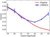 |
Fig. 20 Fraction of galaxies modelled with one component model with respect to the total as a function of i-band magnitude. The red line is the resulting fraction in the Flagship catalogue when the relation in Eq. (19) is used. The blue points with error bars represent the fraction of galaxies modelled with a one-component model in the CANDELS catalogue of Dimauro et al. (2018). |
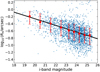 |
Fig. 21 Scalelength values in the HST_GS sample (small blue dots). The red dots indicate the median of the scalelength values in bins of i-band magnitude and the red error bars show the 16 and 84 percentiles of the distributions of scalelengths in each bin. The black line is the fit to the median values of the distribution as a function of the i-band magnitude as given in Eq. (20). |
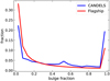 |
Fig. 22 Bulge fraction distribution for galaxies brighter than IE < 24.5 in the Flagship catalogue compared to the CANDELS catalogue of Dimauro et al. (2018) for the same magnitude range. |
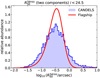 |
Fig. 23 Distribution of half-light radius, |

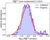 |
Fig. 24 Distribution of half-light radius, |

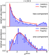 |
Fig. 25 Distribution of Sérsic indices, nSérsic, in the Flagship catalogue for the two-component galaxies (top) and the one-component galaxies (bottom) compared to the CANDELS sample for galaxies with a magnitude limit of i < 24.5. |
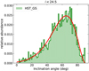 |
Fig. 26 Distribution of inclination angles, θincl , in the Flagship catalogue for the disk component of the two-component galaxies compared to the HST_GS sample for galaxies with a magnitude limit of i < 24.5. |
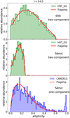 |
Fig. 27 Distribution of ellipticity values, ϵ, in the Flagship catalogue for the disk component (top) and Sérsic component (middle) of the two- component galaxies compared to the HST_GS sample; and the Sérsic component of the one-component galaxies (bottom) compared to the CANDELS sample for galaxies with a magnitude limit of i < 24.5. |
5.6 Galaxy intrinsic alignment
In addition to the shape modelling described in the previous subsection, we model shapes and orientations in a separate process in order to simulate the intrinsic alignment (IA) signal, as detailed in Hoffmann et al. (in prep.).
Our IA model consists of two steps. Approximating each galaxy as a 3D ellipsoid, we assign in the first step two 3D axis ratios to each object, taking into account its redshift, absolute magnitude, and rest-frame colour. The parameters of the shape model component have been calibrated such that the distribution of projected 2D axis ratios matches the observed distribution from the COSMOS survey. The 3D orientations of the galaxies’ principal axes are modelled in a second step, using two different methods for central and satellite galaxies. Centrals are aligned with the principal axes of their host halo, while satellites are pointed towards their host halo centre. These initial orientations are then randomised depending on each galaxy’s redshift, magnitude, and colour, which allows for calibrating the dependence of the resulting IA signal on galaxy properties. Once the 3D axis ratios and orientation have been assigned, the 2D intrinsic shear components are obtained via projection along the observer’s line-of-sight.
A novel feature of the IA model, in comparison to its predecessors, is its calibration against alignment signals derived from multiple constraining datasets through a thorough exploration of the simulation parameter space. At redshifts below z = 0.36 we calibrate against the IA signal measured from luminous red galaxies in the LOWZ sample of the Baryon Oscillation Spectroscopic Survey (Singh & Mandelbaum 2016) as well as samples of red and blue galaxies from the Sloan Digital Sky Survey (Johnston et al. 2019). These low-redshift constraints are complemented by alignment measurements in three magnitude-limited samples at z = 1.0 from the Horizon AGN simulation (Dubois et al. 2014).
Validations of the alignment model are presented in Hoffmann et al. (in prep.). A comparison of the resulting signal against theory predictions are studied in Paviot et al. (in prep.), whereas predictions on the IA parameters for Euclid-like samples are investigated in Tutusaus et al. (in prep.).
5.7 Physical parameters
The Euclid galaxy clustering main probe selects emission line galaxies as the tracers to sample the large-scale structure of the Universe and conduct cosmological inference. In order to compute the emission line fluxes, we first need to estimate other physical properties of the galaxies that the emission lines depend on.
We start by computing the galaxy ultraviolet (UV) photon flux density from the galaxy SED. We integrate the galaxy SED, without the extinction component, derived in Sect. 5.4:
 (38)
(38)
where  is the SED flux density, c is the speed of light, and RUV is a top-hat filter response in the UV with full transmission in the wavelength range from 1500 to 2300 Å and zero transmission otherwise.
The star-formation rate (SFR) is computed from the UV flux,  in Eq. (38) following the relation of Kennicutt (1998) for a Chabrier initial mass function (IMF, Chabrier 2003),
 (39)
(39)
where the constants are for LUV given in erg s−1 Hz−1 units;  , in erg cm−2 s−1 Hz−1; and the luminosity distance, dL, in h−1 Mpc. Equivalently,
 (40)
(40)
We derive the galaxy stellar mass, ℳ, from the galaxy SED and its luminosity. First, we estimate the stellar mass-to-light ratio from the galaxy colours and SED. As our reference band to compute luminosities is the r01 filter (see Sect. 5.1), we estimate the stellar mass-to-light ratio in this band. The stellar mass is then obtained simply by multiplying its r01-band luminosity by the stellar mass-to-light ratio. The galaxy metallicity is computed from the galaxy stellar mass following the relation of Curti et al. (2020), which we slightly modify and extrapolate to cover the whole stellar mass range covered by our sample. We assume a relation for the mean value of the stellar mass-metallicity given by
![Mathematical equation: $12 + {\log _{10}}\left( {{{\rm{O}} \over {\rm{H}}}} \right)({\cal M},{\rm{SFR}},) = 6.7 + {{2.22} \over {1 + \exp \left[ { - 0.85\left( {{\cal M} - {{\cal M}_{{\rm{ref}}}}} \right)} \right]}},$](/articles/aa/full_html/2025/05/aa50853-24/aa50853-24-eq68.png) (41)
(41)
where ℳ is the stellar mass and ℳref is a reference value given by
 (42)
(42)
where SFR is the star formation rate and z, the galaxy redshift. With these relations (Eqs. (41) and (42)), the metallicity depends on the stellar mass, the SFR, and the redshift of the galaxy.
For each galaxy, we draw a realisation assuming a Gaussian distribution of the metallicity values around its mean, with a standard deviation (e.g., Tremonti et al. 2004; Curti et al. 2020)
![Mathematical equation: $\sigma = 0.01 + 0.03\left\{ {8.92 - {{\left[ {12 + {{\log }_{10}}({\rm{O}}/{\rm{H}})} \right]}_{{\rm{mean}}}}} \right\},$](/articles/aa/full_html/2025/05/aa50853-24/aa50853-24-eq70.png) (43)
(43)
where [12 + log10(O/H)]mean is the mean value of the metallicity given by Eqs. (41) and (42).
Figure 28 shows the stellar mass-metallicity relation (MZR) as a function of redshift and SFR in the top panel. The dependence of the relation is stronger on SFR (different colours in Fig. 28) than on redshift (different line styles). In the bottom panel, we show the distribution of a galaxy sample selected at IE < 24.5 and redshift z = 1 in the stellar mass-metallicity space. The red dots show the median of the distribution of metallicities in stellar mass bins, and the error bars the 16 and 84 percentiles of the distribution. Three curves of the MZR for three different values of the SFR at z = 1.0 are also shown. The median values of the metallicities correspond to galaxies with SFR ~ 1 M⊙ yr−1. The dispersion in the distribution, shown by the error bars, takes into account the variations in SFR of the sample and the intrinsic scatter given by Eq. (43). The combination of both gives a standard deviation of the values of the metallicity of ∆ log10 [O/H] ~ 0.07, similar to those found in Curti et al. (2020).
5.8 Galaxy emission lines
The determination of the galaxy redshift with the Euclid NISP instrument (Euclid Collaboration: Jahnke et al. 2025) in slitless mode rely mostly on the identification of emission lines. Therefore, the computation of emission line fluxes is important to understand the completeness and purity of the emission line- selected galaxies that are used for the clustering cosmological probe.
First, we compute the Hα line flux, fHα, from the starformation rate using the Kennicutt (1998) relation adapted to the Chabrier IMF, using the un-extincted UV absolute AB magnitude
 (44)
(44)
where fHα is the flux in the Hα line,  is the unextinguished UV absolute AB magnitude, and dL, the luminosity distance. We add a random scatter following a Gaussian distribution of standard deviation of 0.05 in the logarithm of the flux to the computed logarithmic value of the flux.
Our Hα fluxes are estimated from the UV fluxes that rely on the SED assignment procedure, which is based on observed optical colours (see Sect. 5.4). We then compute the dust- extinguished Hα flux. We get the stellar continuum extinction at the Hα wavelength using the extinction law and colour excess value E(B – V) of the galaxy SED (Sect. 5.4). We then convert the stellar continuum extinction to a nebular emission line extinction using the redshift-dependent factor 0.44 + 0.2 z (Calzetti et al. 2000; Saito et al. 2020), which we clip at 0.44 and 1.0 as minimum and maximum values, respectively, and apply this extinction factor to the Hα flux. We provide both the extinguished and un-extinguished fluxes in our catalogue. Finally, we calibrate the resulting fHα distribution to the Pozzetti et al. (2016) models applying a correction to the computed Hα fluxes with abundance matching to the models. Figure 29 shows the redshift distributions for the simulated samples assuming a flux cut of fHα > 2 × 10⁻¹⁶ erg s−1 cm−2 in the model 1 and model 3 Hα fluxes.
In the SED assignment procedure, we compute each SED as a linear combination of SEDs at fixed redshift values. In particular, we assign the extinction with distributions computed at particular redshifts given in footnote 14. The Hα flux is computed from the unextinguished UV flux. In the process of subtracting the extinction from the SEDs, we introduce discontinuities in the Hα flux-redshift distribution at those particular redshifts. As a temporary fix, we compute a correction of the Hα fluxes to smooth the distributions at those redshifts. In Fig. 29, we can see the performance of this smoothing procedure that was applied at redshifts z > 0.5, but not at z = 0.5 as there is not enough volume in the simulation lightcone to do it properly.
The other hydrogen lines of the Balmer and Paschen series are computed from the Hα flux assuming case B recombination from Osterbrock & Ferland (2006). The [O II] and [O III] fluxes are computed from the Hβ fluxes and the metallicity of the galaxy taking into account the relations of the [O II]/Hβ and [O III]/Hβ flux ratios as a function of metallicity of Curti et al. (2020). The [N II] fluxes are calculated from the [O III]/Hβ flux ratio and the Hα flux following the Baldwin-Phillips-Terlevich (BPT) diagram (Baldwin et al. 1981) using the relations of Kewley et al. (2013a) that include redshift evolution21. The [S II] flux is computed from the Hα flux and the metallicity following the relation of Curti et al. (2020). We obtain the [S III] flux from the [S II] flux and a fit to the relation between the [S III]/[S II] and [O III]/Hβ flux ratios shown by Mannucci et al. (2021) in their Fig. 2. We generate a realisation of all fluxes adding scatter to the value obtained with the relations used. As an example, Fig. 30 shows the position of the Flagship galaxies at z = 1.2 and with Hα flux fHα > 2 × 10⁻¹⁶ erg s−1 cm−2 in this diagram, together with the Kewley et al. (2013a) relation at this redshift.
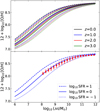 |
Fig. 28 Metallicity as a function od stellar mass, star formation rate, and redshift. Top: Mean values of the metallicity as a function of the stellar mass for different values of redshift (colour code in the figure legend) and SFR (dashed, solid, and dotted lines correspond to log10[SFR/(M⊙ yr−1)] = 1,0, −1, respectively) from Eqs. (41) and (42). Bottom: The red dots show the distribution of median values of the metallicity as a function of stellar mass for a sample at redshift z = 1.0 with magnitude limit IE < 24.5. The red error bars show the 16 and 84 percentiles of the metallicity distributions in each stellar mass bin. The blue lines indicate the mean value of the metallicity-stellar mass relation, Eq. (41), at three specific values of the SFR, as indicated in the legend (that are the same as those in the top panel). |
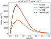 |
Fig. 29 Redshift distribution (galaxies per deg2 per unit redshift) of samples selected with a flux limit cut of fHα = 2 × 10⁻¹⁶ erg s−1 cm−2. The sold lines show the redshift distributions from models 1 (light blue) and 3 (light green) of Pozzetti et al. (2016). The dashed lines are the distributions in the Flagship catalogue for the same flux cut for the model 1 (orange) and 3 (red) simulated fluxes. |
5.9 Galaxy lensing
The implementation of lensing properties on mock galaxies uses the all-sky dark matter lensing maps discussed in Sect. 3. Given this set of 2D maps covering the entire redshift range of the lightcone output of the simulation, our procedure is the same as the one originally implemented in the MICE simulations (Fosalba et al. 2015). This is a simple 3-step algorithm that we describe below.
for a given galaxy at the 3D position in the lightcone
 , where
  gives its angular position in the sky and z its redshift, find the corresponding 3D pixel in the discretised lightcone, with pixel center coordinates,
  , where the galaxy sits in (i.e., the 3D pixel in the suite of ‘onion slices’ or all-sky lensing maps in HEALPix tessellation described in Sect. 3),
get the lensing values for this 3D pixel using the dark matter all-sky lensing maps,
 , where the components of the lensing vector are L = (ĸ,γ1, γ2), which is convergence and shear, and
assign these pixelised dark matter lensing values, Li,j, to the mock galaxy.
The resulting implementation of galaxy lensing using the above method is thus limited by the pixel resolution used, HEALPix Nside = 8192, which corresponds to a pixel scale of 0′.43. Therefore, we only expect to accurately model lensing observables down to ~0′.5 scales, as we will discuss in detail when we validate the mock properties below (see Sect. 6.3). A further limitation intrinsic to this method is that different galaxies falling within a given 3D pixel in the ‘onion universe’ grid pattern of the lightcone have identical lensing properties. These two limitations can be overcome using the same approach but using a finer pixel scale (i.e., higher Nside) and/or using interpolation schemes.
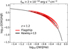 |
Fig. 30 BPT diagram at z = 1.20. The red contours show the density of Flagship galaxies selected with the standard Euclid galaxy clustering sample Hα flux limit of fHα = 2 × 10⁻¹⁶ erg s−1 cm−2 in this diagram. The black solid line is the relation of Kewley et al. (2013a) for this redshift. |
6 Mock validation
Figure 31 shows a small rectangular portion of the Flagship catalogue in the lightcone22. The figure illustrates the breadth of the simulation. It covers a region of 4368 h−1 Mpc (horizontal direction) × 300 h−1 Mpc (vertical direction) with a depth of 80, 160, and 200 h−1 Mpc for the top, middle, and bottom panels respectively, with the observer located in the left-bottom corner. In the top panel we show the dark matter haloes where one can see the growth of structure progressing from right, z = 3, to left, z = 0. The middle and lower panels present likely galaxy samples to be used in the Euclid cosmological analysis. The middle panel shows the galaxies selected with an IE < 24.5 magnitude cut, which we expect to be representative of the weak lensing sample. In the lower panel, we show a sample selected with an Hα flux cut fHα > 10−16 erg cm−2 s−1, trying to mimic the galaxy clustering sample. In the majority of our validation discussion, we refer to samples selected with these observational cuts, since they are the more relevant for the Euclid mission.
6.1 General galaxy properties
In order to assess the performance and possible limitations of the Flagship galaxy catalogue, we compare the galaxy properties, distributions, and relations to observations. In particular, we compare the mock galaxies to observed quantities relevant for the Euclid cosmological probes, including observed galaxy number densities, colours, emission lines fluxes and ratios, as well as sizes at different redshifts.
In Fig. 32, we compare the number counts of the Flagship simulation to literature data and COSMOS2020 (Weaver et al. 2022) counts of magnitudes corrected for Galactic extinction. We show the number density per unit area and magnitude in the IE and HE bands, as well as in similar filters observed in COSMOS, without applying further corrections to account for the differences in the filter transmissions. Also, fluxes and magnitudes from Flagship are intrinsic, while the observed ones are affected by the photometric noise, and their distribution could, therefore, be broader.
In general, we find excellent agreement with observations in the optical band from the brightest to the faintest objects in the mock. We find, however, some differences in the HE band, where the galaxy number density in the mock is about 40% higher than in the literature. At the EWS limit of HE < 24.0 (detection limit at 5 σ for point sources) the integrated number density in the mock is about 188 000 deg−2 compared to ~131 000 deg−2 in the COSMOS field.
In Fig. 33, we also explore how galaxy colours compare with the COSMOS2020 catalogue: the optical (r − i) vs. (u − r) diagram is quite well reproduced at the EWS magnitude limit, with a small offset. The evolution with redshift of the iHSC − HVISTA galaxy colour (a proxy for IE − HE), not used in the input calibration, reproduces the trend observed in COSMOS2020 (for which we are using the photometric redshift obtained with LePhare; Ilbert et al. 2006). However, the Flagship colour distribution presents redder colours than the COSMOS2020 distribution, especially at high redshift. This is an indication, together with the overestimation of the H-band number counts and the good optical number counts and colours, that our near-infrared fluxes are overestimated. Our SED assignment is likely to be the underlying cause for having brighter galaxies in the near-infrared. We assign SEDs based on the g − r optical colour. There is a degeneracy in the optical-to-near-infrared colours (e.g., i − H) that have the same g − r optical colour. We seem to be assigning redder overall SED templates when there is such a degeneracy, causing an overestimation of the near-infrared fluxes. We are exploring new procedures to assign the SEDs to produce colour distributions closer to the ones observed, which we plan to implement in future versions of the catalogue.
In Fig. 34, we show the galaxy stellar mass function (GSMF) derived for the full octant of our Flagship lightcone in various redshift bins. The high resolution of the simulation allows us to derive the GSMF down to very low-mass limits (~108 M⊙) up to z = 3. Comparison to observations in the COSMOS field (Ilbert et al. 2013) shows a good consistency at low redshift z ≲ 2. At higher redshifts, the Flagship GSMF overestimates the abundance for stellar mass galaxies of  . This overestimation at low stellar masses is more evident when comparing to the COSMOS2020 GSMF of Weaver et al. (2023), which extends the Ilbert et al. (2013) GSMF to lower stellar masses. In general, FS2 is fairly consistent with the COSMOS data at the high-mass end, while it shows an excess below the characteristic galaxy mass of
  , especially at redshifts z ≳ 1.5. As mentioned in Sect. 5.7, we compute the galaxy stellar mass from the galaxy luminosity and the stellar mass-to-light ratio. The overestimation of the stellar mass at the low-mass end could either be due to an overestimation of our galaxy luminosity function or to an incorrect assignment of the stellar mass-to-light ratio. The luminosity function that we use is based on the GOODS LF of Dahlen et al. (2005), which we extrapolate to higher redshifts and to lower luminosities (see Sect. 5.1 and Fig. 9). Our extrapolation to the low luminosity range follows the upturn of the faint end of the LF at low redshift (Blanton et al. 2005a), which we extrapolate to higher redshifts. This extrapolation may cause an overestimation of the stellar mass. We also extrapolate the GOODS LF to higher redshifts, z > 2. The high-mass end of the stellar mass function coincides with the observational data at this redshift range, indicating that the extrapolation is apparently adequate at the bright end. The galaxy number cunts (Fig. 32) are consistent with the observational data in the optical, suggesting that our extrapolation of the LF generate galaxies that are consistent with the optical number counts. Our assignment of the stellar mass-to-light ratio may also be overestimated, but this seems more unlikely. Our SEDs seem to be too red in the near-infrared, as suggested by the nearinfrared number counts, which may overestimate the ℳ/L ratio. But since we are using the optical data for estimating the stellar mass-to-light ratio, we think it does not have a significant impact in the GSMF overestimation at the low stellar mass end.
In Fig. 35, we show the SFR mass relation at different redshifts from the simulation computed from the galaxies in an area of about 25 deg2 . The comparison to observational data in the COSMOS field is fairly satisfactory, with a small remaining offset and broader relation in COSMOS, due to the effect of observational uncertainties in recovering properties from the data. We further note that in the Flagship simulation the presence of a quenching population with specific SFR lower than 10−11yr−1 is less evident. We stress, instead, that the Euclid Wide Survey area will allow us to map this relation up to very high stellar masses where previous observations are limited by area and statistics. Future work will provide a detailed comparison with data considering all the instrumental and survey-selection effects, forecasting Euclid performance in recovering different galaxy properties and populations (Euclid Collaboration: Enia et al. 2024).
Besides photometric properties, the most important quantities to validate for the galaxy clustering Euclid cosmological probe are the emission line fluxes and number densities. Figure 36 shows the emission line galaxy densities for a flux limit of fHα + [N II] > 2 × 10⁻¹⁶ erg s−1 cm−2, together with the global EWS limit of IE < 24.5 (10 σ) and HE < 24 (5 σ). We note that in Fig. 36 we have chosen the flux limit in the combination of the Hα and [N II] lines, since these lines are blended with the Euclid NISP grism resolution (Euclid Collaboration: Jahnke et al. 2025). As expected, the Hα emitters spectroscopically observed by Euclid will be only a few percent of the total EWS photometric sample. Finally, as described in Sect. 5.8, we verify that the Flagship mock has been calibrated to the empirical models of Pozzetti et al. (2016). Some differences are still present, when we consider the combination of Hα+[N II], mainly due to [N II] contribution to the total flux, which is assumed constant in the models and not in the Flagship catalogue. In particular, the redshift distribution of fluxes calibrated on model 3 is fairly consistent with the one from Bagley et al. (2020) when we consider a sample limited in Hα+[N II] fluxes to 2 × 10⁻¹⁶ erg s−1 cm−2. From the Flagship catalogue, calibrated on the models 3 and 1 of Pozzetti et al. (2016), we expect that the EWS will map a density of about 3500–6300 deg−2 Hα +[N II] emitters with fluxes above 2 × 10⁻¹⁶ erg s−1 cm−2 in the redshift range 0.9 < z < 1.8, among which about 2000–3800 deg−2 have Hα flux brighter than that same flux limit. In the Euclid Deep Survey (EDS), these numbers increase to about 38 000-55 000 deg−2 in the redshift range 0.4 < z < 1.8 with Hα+[N II] fluxes above 5 × 10⁻¹⁷ erg s−1 cm−2.
We underline, however, that the measurements of galaxy redshift rely mainly on the identification of emission lines and on their ratios. We show in Fig. 37 how our mock catalogue populates the BPT emission line ratio diagram (Baldwin et al. 1981) and how it compares with observations. In particular, we show that we recover quite well the main locus of the BPT diagram from the SDSS galaxy main sample at low redshift (z < 0.3) and also the trend to higher values shown by high-redshift observation in the Fiber Multi-Object Spectrograph (FMOS)-COSMOS survey (Kashino et al. 2019) and by the MOSFIRE Deep Evolution Field (MOSDEF) survey with Keck by Kriek et al. (2015) and Reddy et al. (2015) in the redshift range 1.4 < z < 1.7. Our low-redshift diagram is narrower than the SDSS due to the fact that we do not include observational errors in the line fluxes. We also show other diagrams with various emission line ratios in Fig. 38. In the top panel we present the BPT diagram at 0.9 < z < 1.8, with the [S II] line instead of [N II] line. Our values seem consistent with the FMOS data and have an overall shape similar to the SDSS low-redshift data. In the lower panel we show the [O III]/Hβ ratio as a function of stellar mass. The flagship ratio seems broadly consistent with the FMOS stacked data at similar redshift. The SDSS low-redshift data show low values of the ratio for low stellar mass systems that are not typically found in higher redshift galaxies, which appear to have either high ionisation radiation or lower metal- licity or a combination of both. Overall, these diagnostic plots indicate that the assignment of emission line fluxes is broadly consistent with those observed in SDSS galaxies at low redshift and the FMOS-COSMOS and MOSDEF surveys at higher redshifts. This behaviour is expected, since we are calibrating our line ratios to agree with the BPT relation of Kewley et al. (2013a).
Finally, the weak lensing cosmological probe relies on the measurement of galaxy shapes and sizes. Furthermore, the spectroscopic signal-to-noise ratio of the Euclid slitless spectra depends on galaxy size and, with it, the probability of detecting and measuring emission lines and galaxy redshifts for the clustering cosmological probe. The procedure to assign galaxy sizes distribution was already described in Sect. 5.5 and its comparison to the calibration data shown in Figs. 23 and 24. Additionally, in Figs. 39 we show the distribution of disk sizes of Hα emitters in the redshift range 0.9 < z < 1.6 of a sample limited in flux to fHα+[N II] > 2 × 10⁻¹⁶ erg s−1 cm−2 and compare it to the observed distributions of the slitless spectroscopic HST Wide Field Camera 3 (WFC3) data sets of Bagley et al. (2020). Figure 39 presents the overall histogram distribution of half-light radii of the Flagship galaxies which is consistent with the one observed by Bagley et al. (2020), once observational effects are taken into account. The overall dispersion is similar, even though the predicted median disk size in the FS2 is around 0″.48, compared to 0″.35 in Bagley et al. (2020). Although not shown, the dependence of half-light radius on Hα+[N II] flux is similar in both samples. The overall half-light radius distribution difference can be explained by a selection effect, as the detection probability is dependent on galaxy size, with more compact galaxies having a higher probability of being detected. We performed a preliminary comparison of the predicted size distribution under this selection effect, obtaining a consistent shift in the size distribution. The description of the techniques needed to perform this test is beyond the scope of this paper. The details of the selection procedure and its dependence on galaxy properties will be presented in Euclid Collaboration: Monaco et al. (in prep.).
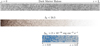 |
Fig. 31 Flagship galaxy catalogue: stripes show sections of the lightcone for z < 3 for dark matter haloes (top panel), the photometric sample for IE < 24.5 (middle), and an Hα spectroscopic galaxy sample for a flux cut fHα > 2 × 10⁻¹⁶ erg cm−2 s−1 (bottom), which selects galaxies only within the range 0.9 < z < 1.8 given the NISP red grism wavelength coverage. The stripe abscissae share the same scaling in comoving distance. The colour scaling in each panel depends on the density of the sample. |
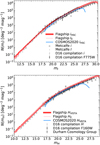 |
Fig. 32 Galaxy number densities in the IE and HE bands compared to literature data: COSMOS2020 (Weaver et al. 2022) counts in HVISTA and iHSC are derived from the ‘farmer’ version of the photometric catalogue, after removing masked regions and objects classified as stars; Driver et al. (2016); Durham Cosmology Group’s counts are from the compilation available at the dedicated web page (http://star-www. dur.ac.uk/~nm/pubhtml/counts/counts.html). |
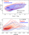 |
Fig. 33 Galaxy colour-colour and colour-redshift diagrams compared to COSMOS2020 data. In the optical wavelength range, our colour-colour diagram seems consistent with the COSMOS2020 data, while our i – H colours indicate that our galaxies are redder than what is observed in this colour combination, especially at z > 0.5. |
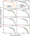 |
Fig. 34 Galaxy stellar mass function at different redshifts. In red the GSMF derived from the Flagship lightcone compared to GSMF derived at z < 0.1 in GAMA (Driver et al. 2022, yellow line) and at higher redshifts in COSMOS from the ULTRAVISTA sample (Ilbert et al. 2013, green squares), and the COSMOS2020 release (Weaver et al. 2023, blue lines). We have transformed the Flagship stellar masses to units of the Hubble constant of H = 70 h70 km s−1 Mpc−1 to bring the units of the Flagship catalogue to the ones used by the other surveys. |
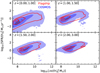 |
Fig. 35 Galaxy star-formation rate – stellar mass relation at different redshifts. The Flagship lightcone catalogue (red empty contours corresponding to the 5, 50, and 90 percentiles of the distribution) is compared to COSMOS2020 (Weaver et al. 2023, blue levels at the same percentiles). |
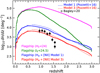 |
Fig. 36 Expected number densities for photometric and spectroscopic emission line flux selected samples as a function of redshift in the Euclid Wide Survey. Different colours show various selection cuts for the EWS (in IE , HE , and in the 2 model calibrations for the line fluxes of fHα+[N II] > 2 × 10⁻¹⁶ erg s−1 cm−2). The empirical model of Pozzetti et al. (2016) and the data based on slitless HST spectroscopy (Bagley et al. 2020) are also shown. |
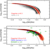 |
Fig. 37 BPT diagram. Top panel: emission line ratios in the redshift range z < 0.5 for Flagship (red colour map) compared to SDSS (in grey) main target sample for objects classified as galaxies. Bottom panel: emission line ratio in the redshift range 0.9 < z < 1.8 compared to FMOS stacked data in COSMOS at z ~ 1.5 from Kashino et al. (2019) and MOSFDEF data from Kriek et al. (2015) and Reddy et al. (2015). The black lines are the relations by Kewley et al. (2013a) at z ~ 0 (dotted lines) and z ~ 1.5 (solid lines). |
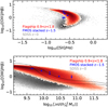 |
Fig. 38 Emission lines ratios in the Flagship simulation. Flagship galaxy fluxes (red colour map) compared to SDSS fluxes (grey map) from the main target sample for objects classified as galaxies in the local Universe. In blue, we also show FMOS stacked data in COSMOS from Kashino et al. (2019). Top panel: [O III]/Hβ versus [S II]/Hα. Bottom panel: [O III]/Hβ versus stellar mass; the thin dotted curves indicate the divisions between star-forming/composite galaxies and AGN at z ≃ 0 (Juneau et al. 2014), with AGN populating the region of larger [O III]/Hβ above the dotted lines. |
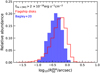 |
Fig. 39 Size distribution. Disk half-light radius distribution of an Hα selected sample, at the limit of the EWS in the redshift range 0.9 < z < 1.6, compared to data from Bagley et al. (2020). |
6.2 Galaxy clustering
The clustering properties of the FS2 galaxies were tested at various levels, to check the stability of clustering for objects produced in various steps along the pipeline. To this aim we selected four classes of objects, identified so as to follow the main step of the catalogue construction (the thresholds are chosen to have a similar level of clustering in the first of the redshift bins defined below): (i) dark matter haloes on the lightcone more massive than Mh = 1012 h−1 M⊙ (the starting point), (ii) galaxies with absolute r-band magnitude brighter than Mr − 5 log10 h = −20 (after application of HOD+AM, Sect. 5.1), (iii) galaxies with apparent magnitude HE < 22 (after SED assignment, Sect. 5.4)23, (iv) emission line galaxies (ELGs) with Hα line flux greater than fHα = 2 × 10⁻¹⁶ erg s−1 cm−2 (after emission lines assignment, Sect. 5.8). For each selected catalogue we consider the four redshift bins expected to be used for the analysis of the spectroscopic sample, namely [0.9,1.1), [1.1,1.3), [1.3,1.5), and [1.5,1.8). To isolate the effect of peculiar velocities in redshift-space distortions, we select comoving angles (instead of magnified angles, which are shifted according to the gravitational lensing displacement field), observed redshift containing the contribution from background expansion and first-order peculiar velocities, and an unmagnified flux cut. This ensures that our measurements are not affected by lensing effects, which have been shown to be non-negligible for high-redshift 3D galaxy clustering (Jelic-Cizmek et al. 2021; Breton et al. 2022; Euclid Collaboration: Jelic-Cizmek et al. 2024) and whose effect is outside the scope of this paper. For each catalogue, we generate an associated random catalogue constructed by replicating the galaxy catalogue 50 times, keeping the redshift while assigning random sky positions within the angular footprint of the mock survey (an octant of the sky). This way, the average number density of the random reproduces exactly 50 times that of the galaxy catalogue.
First, we report our validation of the galaxy clustering probe in Fourier space using the official code developed to compute the power spectrum (PK) in Euclid (Euclid Collaboration: Sefusatti et al., in prep.), based on the Yamamoto-Bianchi estimator (Bianchi et al. 2015). The code accepts a catalogue with (cosmology-independent) angular coordinates and redshift; we computed the monopole of the real-space PK, obtained by providing the true redshift of the galaxy, and the first three odd multipoles of the redshift-space PK, obtained by providing the ‘observed’ redshift that includes peculiar velocities. The same PK code performs a measurement of the power spectrum of the randoms, which is used to create a model of the window function.
The measured power spectra were fitted with a model based on a standard perturbation theory (SPT) at 1-loop with effective field theory (EFT) counter-terms using the PBJ code presented by Moretti et al. (2023). Cosmological parameters were fixed to those used in the simulation. This model contains the following parameters for galaxy bias, shot noise, and EFT that were used as nuisance parameters: b1 (linear bias), b2 (quadratic bias),  (second order Galileon bias), c0 and c2 (the EFT counterterms), αP (deviation from the Poisson shot-noise),
  dependent shot-noise), and
  (Finger-of-God counter-term). In redshift space we left the growth rate f free and added Alcock– Paczynski (AP) free parameters α|| and α⊥ to the fiducial power spectrum. Indeed, the aim here is not to perform accurate cosmological inference from the spectroscopic catalogue but to check that we can infer the input cosmological parameters consistently when using the different catalogues along the mock production pipeline. The model was convolved with the window function following the matrix multiplication method of d’Amico et al. (2020). For the covariance matrix we used a simple analytic Gaussian, leading-order covariance; to minimise the impact of this naive choice and the lack of a proper convolution with the window function, we binned the power spectrum in bins of 8 times the fundamental frequency (kf) of the box used for the measurement (Lbox = 10 h−1 Gpc), so that
  , where Veff is the effective survey volume. The model range of validity is thus from kmin = 8 kf = 0.005 h Mpc−1 to kmax = 0.2 h Mpc−1. For the likelihood, we neglected the hexadecapole, which had a negligible effect on the posteriors.
First, the real-space PK was fitted by the model with fixed cosmological parameters, with the aim of obtaining the b1 linear bias parameter of the four classes of objects. In the second stage, we fitted the redshift-space PK of the four catalogues, leaving f, α|| and α⊥ free. Figure 40 shows the PK measurement of the monopole, quadrupole, and hexadecapole of the four samples in the first redshift bin, [0.9,1.1]; we also report the best-fit model PK of the Hα ELGs. Figure 41 shows the resulting cosmological parameters obtained from the four samples, together with linear bias b1 ; posteriors are marginalised over the other nuisance parameters. The cosmological posteriors are very stable when varying the sample and are compatible to within 1 σ with the true values, amounting to 1 for the AP parameters and to f = 0.9 for the growth rate (computed for the median redshift z = 1); the small bias obtained for some of the parameters raises no concern as we are using a single realisation and a simplified treatment of the covariance. The variation of parameter error bars for the four catalogues is very limited, and this is due to the fact that at k = 0.2 h Mpc−1 the power spectrum is still well above the shot noise level in all cases, so the different number densities of the samples do not influence much the parameter error bars in this regime. Linear bias, b1 , values are compared with those obtained from real space (dashed lines). In this case, we also obtain a very moderate bias in this measurement, which is very consistent for all the samples. In conclusion, the various steps in the definition of the galaxy sample do not bias the inferred cosmological parameters.
We now focus on the multipoles of the two-point correlation function for Hα galaxies in redshift space. To estimate the correlation function we use the LS estimator (Landy & Szalay 1993)
 (45)
(45)
where NDD , NDR, and NRR respectively stand for data-data, data-random, and random-random pair counts that we estimate with Corrfunc24 (Sinha & Garrison 2020), in bins of s the comoving pair separation (between 25 and 150 h−1 Mpc) and µ the cosine of its angle (using the mid-point definition) with respect to the line of sight. To estimate the multipoles of the correlation function we integrate the 2D correlation function as
 (46)
(46)
where ℓ is the multipole and ℒℓ the ℓ-th order Legendre polynomial. We integrate µ from 0 to 1 due to symmetry along the line of sight when using auto-correlations and the mid-point definition, which is µ = r ⋅ s/ (rs), where r = (r1 + r2)/2 and s = r2 − r1, with r1 and r2 the vectors of the galaxy positions.
We compare our measurements to a theoretical prediction based on EFTofLSS (Ivanov et al. 2020; d’Amico et al. 2020) as implemented in COMET (Eggemeier et al. 2023). To obtain the prediction, we first produced Gaussian covariance matrices for each redshift bin following the recipe from Grieb et al. (2016). Once we compute a covariance with a model which fits the data, we run Monte Carlo Markov chains (MCMCs) using PyMultinest (Buchner et al. 2014). Consistent with the power spectrum analysis presented above, we performed a fixed- template fit assuming the fiducial cosmology of the simulation and varying f the growth rate, α|| and α⊥ the dilation parameters, the linear and quadratic biases (higher-order biases are fixed assuming the local-lagrangian approximation), and EFT counterterms. In principle, it is possible to vary σ12 (the variance of density fluctuations in spheres of 12 Mpc, see Sánchez 2020), but we instead fix it to its fiducial value so as to avoid large degeneracies in the estimation of the linear bias.
The simulation measurements and best-fit model shown in Fig. 42 display a very good agreement, especially for the highest- redshift bins (with mean redshift z = 1.4 and z = 1.65). For the low-redshift bins, it seems that the quadrupole is underestimated by the model at scales above 90 h−1 Mpc. This does not look particularly worrying given that these scales are not independent and that the discrepancy stays between 1 and 2 σ. We also note that for z = 1, the monopole is close to zero at 80 h−1 Mpc, which could be attributed to sample fluctuations in the redshift bin for our simulation realisation.
Finally, we show a simulation-based estimation of the linear bias as a function of redshift in Fig. 43. Different models (linear theory or EFT) in different configurations (real or redshift space, Fourier or configuration space) give very similar results. Because the measurement of b1 from a galaxy sample is not a trivial task, this result can be considered as a validation not only of the simulation itself but also of our analysis pipeline. Nevertheless, our estimate of the bias in either real or redshift space appears to be higher than others reported in the literature, such as the simulation-based forecasts for future missions in Merson et al. (2019) and Zhai et al. (2021a,b). Those results are derived from semi-analytic models of galaxy formation and evolution, which have been calibrated to match the number density of Hα emitters. The methodology employed in these studies differs significantly from the approach used in constructing the Flagship simulation in this work. The extrapolation to clustering measurements may introduce additional uncertainty into the estimated bias, and thus we do not expect great consistency between the analyses. However, the collection of ELG data by Euclid is expected to provide tight constraints on these parameters in the near future.
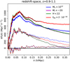 |
Fig. 40 Monopoles (thick continuous lines), quadrupoles (thin continuous lines), and hexadecapoles (dotted lines) of the measured redshiftspace PK for the four samples reported in the legend. The monopole includes shot noise. Thin black lines give the best-fit model (convolved with the window function) for the monopole and quadrupole of the Hα ELG sample. The absolute magnitude-limited sample, Mr − 5 log10 h < −20, in magenta is hardly seen as it has very similar clustering amplitude and is below the magnitude-limited sample, HE < 22, in green. |
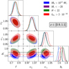 |
Fig. 41 Inferred cosmological parameters (redshift-space f and AP parameters) for the four samples, together with linear bias b1, in the redshift bin [0.9,1.1]. As in Fig. 40, the absolute magnitude-limited sample, Mr − 5 log10 h < −20, contours in magenta are hardly seen as they are very similar and are below the magnitude-limited sample, HE < 22, contours in green. |
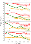 |
Fig. 42 Redshift-space two-point correlation function multipoles of Hα galaxies (points and error bars), and best-fitting prediction using the EFT model (solid lines). Green, red, and orange points refer to monopole, quadrupole and hexadecapole respectively. Different panels show the results for different redshifts as labelled. |
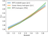 |
Fig. 43 Linear galaxy bias, b1, as a function of redshift for Hα emitters in the Flagship simulation. In blue we show the estimation from the fit to the two-point correlation function multipoles in redshift space using the EFT model. In orange, we use linear theory in real space to fit the correlation function monopole. Finally, in green we fit the real- space monopole of the power spectrum using EFT at one-loop order. The colour bands show the 1 σ confidence regions of the linear bias. |
6.3 Galaxy weak lensing
6.3.1 Main observables: shear 2-point statistics and galaxy-galaxy lensing
Galaxy weak lensing is one of the two main cosmological probes of Euclid. The standard summary statistics used for weak lensing include the shear 2-point correlation functions, ξ±, which in turn are related to the tangential and cross-component of the shear,
 (47)
(47)
where θ is the separation between ϑ and ϑ′, and γt and γ× are the tangential and cross-component of the shear, defined by γt(ϑ) = −ℜ[γ(ϑ)e−2iϕ] and γ×(ϑ) = −J[γ(ϑ)e−2iϕ], where ϕ is the polar angle of ϑ − ϑ′.
In the weak lensing limit these shear correlations are related to the gradient or E-mode component of the shear angular power spectrum (i.e, the B-mode component is typically negligible: see Bartelmann & Schneider 2001; Hilbert et al. 2009),
 (48)
(48)
being  , J0/4 are the Bessel functions of the first kind of order 0 and 4 respectively. where we have assumed no B-modes, and the validity of the Limber approximation (e.g., LoVerde & Afshordi 2008). Another basic observable is given by the galaxygalaxy lensing, or the average tangential shear of a background galaxy sample produced by the foreground matter distribution, 〈γt〉, which is directly related to the cross power spectrum of the convergence field of the background galaxies and the foreground galaxy number counts,
  (see Jeong et al. 2009),
 (49)
(49)
where we have taken the flat-sky limit, which is very accurate for practically all angular scales (e.g., θ < few degrees). The exact expression can be obtained by replacing the integral over ℓ by a sum over discrete ℓ modes, and features Wigner d matrix elements (Chon et al. 2004; de Putter & Takada 2010).
In this section we provide a validation of these basic weak-lensing statistics which are, along with galaxy clustering correlations, the two main cosmology probes of Euclid. Figure 44 shows the simulation measurements of the shear correlation functions at source redshifts ɀ = 1,2, using the athena code25 (Kilbinger et al. 2014) compared to theory predictions from Halofit (Takahashi et al. 2020). The mock galaxy sample has been cut at the nominal magnitude limit of the photometric galaxy sample, IE < 24.5. The measured correlations are in agreement with theory predictions to within 10% down to highly nonlinear scales, i.e, 1‘ for ξ+ (5′ for ξ−). A similar level of agreement between measurements and theory is found for other redshift slices 0.95 < ɀ < 1.05, 1.95 < ɀ < 2.05, and 2.9 < ɀ < 3, as displayed in Fig. 45. We have also compared mock measurements of the galaxy-galaxy lensing, obtained with athena, with theory predictions that use Halofit for the nonlinear matter power spectrum rescaled with a simple linear galaxy bias model. As shown in Fig. 46 we get good agreement within 10–15% for this simple model even on small (nonlinear) scales. Figure 47 shows a comparison of the galaxy-galaxy lensing estimator for different lens-source ɀ-bin pairs across the simulation redshift range. It shows that overall there is good agreement between the simulation and nonlinear theory predictions, except for the smallest angular scales, where the linear galaxy bias model is expected to break down.
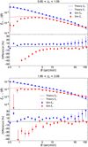 |
Fig. 44 Shear correlation functions for source samples at ɀ = 1 (top), ɀ = 2 (bottom). Simulation measurements (symbols) are compared to linear and nonlinear (Halofit) theory predictions (lines). Errors are obtained from jackknife resampling. The bottom sub-panels show fractional differences between simulations and nonlinear theory. |
6.3.2 Magnification bias
Gravitational lensing by large-scale structures in the Universe changes the number density of background sources and thus it induces a cross-correlation signal between background and foreground galaxy populations (Moessner & Jain 1998; Bartelmann & Schneider 2001). For a magnitude limited survey, the cumulative number of galaxies above a flux limit f scales as N0(> f) ∼ Afα, where A is the area of the survey, and α is the power-law slope of the background number counts. Lensing preserves the surface brightness of galaxies by increasing the observed survey depth (i.e, decreasing the effective flux limit) and the effective survey area by the same amount: f → f /µ, A → A/µ, where µ is the magnification. These two competing effects induce the so-called magnification bias in the cumulative number of background sources,
 (50)
(50)
We define the logarithmic slope of the background number counts at redshift ɀ, for a magnitude limit m, as
 (51)
(51)
In the weak-lensing limit, µ = 1 + δµ where |δµ| ⪡ 1, and we can Taylor expand, µα−1 ≈ 1 + (α − 1)δµ, and therefore the magnified overdensity of background sources is given by,
 (52)
(52)
 (53)
(53)
where in the last equality, we have identified δµ = 2 δκ, which is valid in the weak-lensing limit. We note that in δall we have defined the two qualitatively different contributions:
magnified magnitudes, δm = αδµ,
magnified or lensed positions, δp = −δµ.
These two contributions cannot be separated observationally, but we define two different galaxy samples accordingly in our simulation in order to validate the two magnification contributions separately.
The net magnification from these two competing effects depends on how the loss of sources due to the area dilution, δp, is compensated by the gain of sources from the flux magnification, δm . Number counts for source populations with flat luminosity functions, such as faint galaxies, decrease due to magnification, whereas sources with steep luminosity functions, such as quasars, increase. In the particular case when s = 0.4, then α = 1, and there is no net magnification effect.
For the implementation of the magnification in the flux (or magnitudes) and the galaxy positions, we follow Fosalba et al. (2015) and we refer to that paper for further details. Below we just provide the main definitions.
-
Magnified magnitudes: flux magnification makes the mock galaxy magnitudes, m, brighter by an amount
 (54)
(54)where in the last equality we have Taylor expanded log10(1 − δµ) and used the fact that δµ ≃ 2 κ in the weak-lensing limit. Therefore, knowing the value of the convergence, κ, at a given point in the source plane, it is straightforward to compute the flux magnification induced, which in turn produces the change in the background number counts, δm.
-
Magnified or lensed positions: the ‘observed’ or lensed position, β, of a light ray is shifted from the ‘true’ or unlensed position, θ, by an angle given by the scaled deflection vector, α, according to the lens equation on the source plane (see e.g., Bartelmann & Schneider 2001). In the single-plane (or Born) approximation, the lens equation reads
 (55)
(55)where the deflection vector, α is a tangent vector at the unlensed position of the light ray, and the lensed position is found by moving along a geodesic on the sphere in the direction of this tangent vector and for an arc length given by the scaled deflection angle, α. If we denote the unlensed position on the sphere by (θ, ϕ), then the lensed position, (θ′,φ + Δφ), can be simply derived by using identities of spherical triangles (Lewis 2005).
Figure 48 shows the measured magnification bias b = 5 * s − 2, Eq. (53), where s is the slope of the background galaxy number counts, see Eq. (51), as a function of magnitude limit in the visible (IE) and of redshift. We find that the smooth evolution of s with the magnitude limit applied can be well fitted with a third-order polynomial,  for a given source redshift bin. Table 3 gives the coefficients of the polynomial fit for a set of source redshift bins with width Δɀ = 0.1 up to ɀ = 1.8.
In order to validate the magnified or deflected positions of mock galaxies, we use the estimator for ‘sample variance free’ cross-correlations between background and foreground mock galaxy samples (see Section 5.2 of Fosalba et al. 2015). As shown in Fig. 49, the measured cross-correlations are in good agreement with theory expectations and above the estimated noise level for most of the angular scales probed.
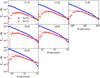 |
Fig. 45 Shear cross-correlation functions for samples at three different source bins 0.95 < ɀ < 1.05, 1.95 < ɀ < 2.05, and 2.9 < ɀ < 3. Panels show all possible cross-correlation ɀ-bin pairs. We denote a ɀ-bin pair with e.g., (1, 2) when correlating shear amplitudes from the ɀ ≃ 1 and ɀ ≃ 2 source bins. The blue points and lines correspond to the ξ+ measurements and theoretical expectations, respectively, and the ones in red to ξ−. |
6.3.3 Higher-order lensing statistics
We also validate the agreement of the third-order aperture statistics  in the Flagship simulation with theoretical predictions. The
  values are the third moments of the aperture mass and therefore depend on the matter bispectrum. They can be inferred in two ways (Schneider et al. 2005): either from maps of the lensing convergence or by first measuring the third-order shear correlation functions and then convolving them with a suitable kernel function. By comparing the results of these two approaches with theory, we can simultaneously test the skewness of the convergence maps and the third-order statistics of the shear catalogues.
For our model, we use the approach in Heydenreich et al. (2023), based on the bihalofit bispectrum (Takahashi et al. 2020) and the aperture filter function by Crittenden et al. (2002). This model has an expected accuracy of 10% for the aperture radii we consider here (Heydenreich et al. 2023).
We measure  on the convergence map at source redshift ɀs = 0.996. For this, the convergence is convolved with the aperture filter for (4′, 8′, 16′, 32′) using Fast Fourier Transforms to obtain aperture mass maps. Then, a border of width 4 × 32′ = 128′ is cut from each aperture mass map to avoid border effects. Finally, the mean of the product of three maps gives
  (θ1,θ2,θ3).
We also measure  from the shear of galaxies at redshifts between 0.984 and 1.01 with a Euclid-like magnitude cut of IE ≤ 24.5. For this we measure the shear three-point correlation function with TreeCorr (Jarvis et al. 2004) for galaxy separations between 0′.1 and 400′, and convert to
  according to Schneider et al. (2005). The correlation function is measured individually for 40 patches, allowing for a jackknife estimate of the variance.
Figure 50 shows the measurement results and the model. The measurements for both methods agree with the model within the 10% model accuracy. They also agree with each other within the jackknife uncertainty. This confirms that the third moment of the matter distribution corresponds to theoretical expectations and that the galaxy shear catalogues retain the correct third-order moment.
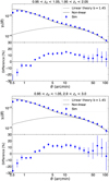 |
Fig. 46 Galaxy-galaxy lensing: cross-correlations between lens positions and source shear for different source redshift planes (ɀs ≃ 2 in the top panel, and ɀs ≃ 3 in the bottom panel, respectively) at fixed lens (deflector) redshift, ɀd ≃ 1. Simulation measurements (filled blue circles) are compared to linear and nonlinear theory predictions (lines). Lower panels show fractional differences between simulation and nonlinear theory. |
6.4 Galaxy clusters
In this subsection, we concentrate on the properties of galaxies in clusters. For this purpose, we consider as ‘clusters’ all haloes more massive than 1014 h−1 M⊙. For computational ease, we concentrate on statistics extracted from a 49 deg2 square region of the Flagship catalogue, which is statistically representative of the whole population for the comparisons we present below.
Figure 51 displays the number of galaxies as a function of cluster halo mass, computed in three ways: for the EWS limits of IE < 24.5 (diamonds) and HE < 24 (circles), and for the Hα flux limit of f (Hα) > 2 × 10⁻¹⁶erg s−1 cm−2 (triangles). At a given redshift, the number of galaxies per halo increases with halo mass, as expected from the HOD approach implemented in the mock. Also, at given halo mass, the number of galaxies per halo decreases with increasing redshift because of the broadband or emission line flux limits. Also, the number of galaxies with potentially detectable Hα emission lines, in the red grism redshift range 0.9 < ɀ < 1.8 is of the order of 5 to 20 per halo, amounting to roughly 6% (0.9 < ɀ < 1.3) and 12% (1.3 < ɀ < 1.8) of the number of galaxies with HE < 24 at those redshifts. Finally, there are no Hα flux-limited selected galaxies in haloes of mass log10[Mh/(h−1 M⊙)] > 14.5, as there are no star-forming blue galaxies in those massive clusters (see Sect. 5.2).
Figure 52 shows the three-dimensional galaxy density profile (top panel) and its slope (bottom panel) for an ensemble sample of 420 haloes selected with the same criteria as in Fig. 17 (0.6 < ɀ < 1.0, 14.0 < log10[M/(h−1 M⊙)] < 14.4, Ie < 24.5, and HE < 24). In the top panel we show the density profile for all galaxies in the catalogue as red points joined by a red line. We also show the density profile for the satellite galaxies belonging to the haloes (located out to 3 virial radii) as a blue line and the field galaxies outside the selected high-mass haloes as a green line. The profile for all galaxies shows a jump at r = rvir due to the fact that we have populated with galaxies the haloes beyond their virial radius and at those radii there are already galaxies from haloes surrounding the high-mass selected haloes that correspond to what we might call the field population. This is also seen in the bottom panel, where we show the slope of the density profile together with the slope of the best-fit NFW profile. At r = rvir there is a clear jump in the density profile slope due to the mixing of the satellite and field galaxy populations. There is a hint of the splashback radius (e.g., Adhikari et al. 2014; Diemer & Kravtsov 2014; O’Neil et al. 2021) at around 2 virial radii, where the slope drops. We also plot how the slope would change if we exclude the satellite galaxies beyond the virial radius when we compute the slope. This exercise of not counting the satellites is only approximate, since we have not properly taken into account the triaxiality of the haloes. Nevertheless, it shows that when we remove the halo satellite galaxies, the splashback radius is more prominent and is located at a lower value of the scaled radius. From the previous analysis, it is clear that we are overpopulating the outskirts of our haloes. We will correct this in future versions of our catalogue. Fortunately, this overpopulation does not significantly affect the clustering statistics of the samples to be selected for the main Euclid cosmological analysis as we have shown in our previous clustering validation analysis. Most of the galaxies used for cosmological analysis belong to lower mass haloes where, given the low number of satellites, there are practically no satellites placed beyond the virial radius.
Figure 53 compares the Flagship line-of-sight velocity dispersion as a function of halo mass with that measured in a 7 deg2 lightcone extracted from the GAEA semi-analytical model (Hirschmann et al. 2016). The agreement between the Flagship and the semi-analytical model is excellent. This indicates that the velocities of Flagship, which follow analytical prescriptions (Sect. 5.3) are fairly realistic, because the galaxy velocities in GAEA are those of the subhaloes as extracted from the dark matter-only simulation on which the GAEA semi-analytical model was extracted. This agreement is robust to the different virial definitions (the ROCKSTAR bound halo virial mass following the Bryan & Norman 1998 definition for Flagship vs. M200c for GAEA). The  and
and  lines (which by definition both have slopes of 2/3) only serve as a reference and are not theoretical expectations.
Figure 54 compares the IE-band cluster luminosity functions (LFs) of Flagship in three redshift bins with the Schechter (1976) function fits performed by Sarron et al. (2018) on clusters using i-band galaxy luminosities from the Canada France Hawaii Legacy Survey (CFHTLS). Both analyses are done for I- band magnitudes brighter than 23. The Flagship LF reproduces reasonably well the observed one, given the intrinsic differences in the LF modelling technique, as well as the different split: by colours in the Flagship catalogue, versus by morphologies in CFHTLS. The numbers of faint galaxies (absolute magnitude between –19 and –21) in Flagship are similar to those predicted by the LF fits to the CFHTLS data. In particular, faint galaxies tend to be blue in both CFHTLS and Flagship, while the red galaxy LF peaks in both, indicating a faint-end slope shallower than -1. However, one sees several differences. The blue Flagship galaxies are less frequent than are the late-type galaxies (LTGs) in CFHTLS at intermediate luminosities at all redshifts. In contrast, the red Flagship galaxies are more frequent than early-type galaxies (ETGs) in CFHTLS at intermediate luminosities at all redshifts and at low luminosities for low redshifts. One expects that the normalisation of the LF will be lower in the Flagship catalogue compared to CFHTLS, since the cylinders used for the galaxy counts are much longer in the Sarron et al. (2018) analysis of CFHTLS, which relied on photometric redshifts. Most outliers are in the field and are more likely to be blue, giving indeed a higher LF in CFHTLS for blue galaxies. Since nearly half of the blue galaxies within the virial cylinder are outside the virial sphere (Mahajan et al. 2011), one expects a little less than a factor of 2 enhancement of the number of blue galaxies in CFHTLS relative to the simulation, which is consistent with Fig. 54. On the other hand, red interlopers should be rarer than blue ones, but should still lead to a somewhat higher LF for CFHTLS compared to Flagship, especially since the Green Valley galaxies in Flagship are not considered here. This is not what is seen in Fig. 54. This excess of red galaxies in the Flagship catalogue may simply mean that red galaxies are more frequent than ETGs, because dust reddening causes edge-on spirals to appear red. Thus, Fig. 54 is consistent with our expectations.
Figure 55 shows the Flagship colour-magnitude relations for field and cluster galaxies, using proxies for rest-frame U − B colours and rest-frame B magnitudes at selected redshifts where the 4000 Å break lies in between the two considered wavebands for the colour, so as to emphasize the separation between Red-Sequence and Blue-Cloud galaxies. One sees that Flagship nicely reproduces the bimodality of colours at ɀ = 0.1, although the Red Sequence is barely visible for the field galaxies, because the Blue-Cloud galaxies are so dominant. This trend is also visible at higher redshifts, showing that cluster galaxies in the Flagship catalogue are more likely to be luminous and red at all redshifts. Again, the Red Sequence is present by construction in all galaxies (blue contours), but is overshadowed by the dominant Blue Cloud.
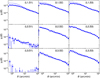 |
Fig. 47 Average tangential shear for source samples in redshift bins (S1, S2, S3) = (0.95 < ɀ < 1.05,1.95 < ɀ < 2.05,2.9 < ɀ < 3), around the lens redshift slices (L1, L2, L3) = (0.45 < ɀ < 0.55,0.95 < ɀ < 1.05,1.45 < ɀ < 1.55. Panels show all possible combinations of cross-correlations between lens sample positions and source galaxy shear. Lens sample redshifts increase from top to bottom panels, whereas source redshift increases from left to right. Solid lines show a fiducial theory prediction for the nonlinear dark-matter power spectrum rescaled with a best-fit linear galaxy bias for the lens samples, b(L1) = 1.2, b(L2) = 1.45, b(L3) = 2.0. |
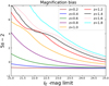 |
Fig. 48 Magnification bias for magnitude-limited source galaxy samples with redshift bin-width Δɀ = 0.1. |
Fitting functions for the slope of the galaxy number counts vs. magnitude cut,  , for different source redshift bins, zs .
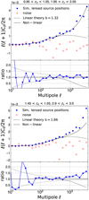 |
Fig. 49 Lens-source cross-correlations as a test of source galaxy position deflections. We show two different lens-source ɀ-bin pairs for galaxy samples cut at IE < 26: a case with ɀd ≃ 1 and ɀs ≃ 2 in the top panel, ɀd ≃ 1.5 and ɀs ≃ 3 in the bottom panel, respectively. Flagship measurements (filled blue circles) are compared to linear and nonlinear theory predictions (lines). Lower panels show the ratio of FS2 measurements over nonlinear theory prediction. Sample variance errors around nonlinear theory are displayed as dotted lines. Cross-correlation in absence of magnification (i.e, noise estimate) is shown as open red circles. The FS2 measurements use an estimator that roughly cancels sample-variance (see text for details). |
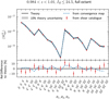 |
Fig. 50 Third-order aperture mass statistic. Top: measured from the convergence map at ɀs = 0.996 (blue, dashed), measured from the shear of galaxies at 0.984 < ɀs < 1.01 (orange points), and modelled (black, solid). Bottom: relative difference of measurements to theory. |
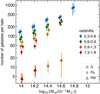 |
Fig. 51 Arithmetic means of the number of galaxies per halo as a function of halo mass. The colours indicate the redshifts, while the symbols indicate the selection: IE < 24.5 (diamonds), HE < 24 (circles), and Hα flux > 2 × 10⁻¹⁶erg s−1 cm−2 (triangles, limited to the redshift range, 0.9 < ɀ < 1.8, where the red grism can see the Hα line). We requested at least 2 clusters per cell of redshift and log halo mass. The error bars show the standard deviations of the numbers of galaxies per halo. The abscissae are slightly offset for clarity. |
7 Summary and conclusions
We have presented the Flagship galaxy mock, a large simulated catalogue especially designed for the Euclid mission. Euclid uses weak lensing and galaxy clustering as its main observables to infer cosmological parameters. The Flagship catalogue simulates these observables in a self-consistent manner and covers the volume and depth required for Euclid. We also compute many other properties for each galaxy to increase the science cases that can be addressed with the catalogue.
We ran a 4 trillion particle dark matter N-body simulations in a box of 3600 h−1 Mpc length side at the Swiss National Supercomputing Centre. We generated a lightcone on the fly out to redshift ɀ = 3 in one octant of the sky containing 31 trillion particle positions and velocities. We have checked that the dark matter clustering properties behave as expected from theoretical predictions.
We also produce an all-sky lensing map in HEALPix format with Nside = 8192 resolution, corresponding to 0′.43 per pixel. From these maps, we can compute the convergence, shear and displacement at any position in the simulation lightcone. The lensing statistics are in general agreement with expectations from theoretical predictions.
We produce a halo catalogue with the ROCKSTAR halo finder of 15.8 billion main haloes in one octant of the lightcone. In order to push the completeness of the catalogue to faint magnitudes as to be complete for the Euclid magnitude selection limit at low redshift, we select haloes down to a threshold of 10 particles, before discarding unbound particles. After the unbinding process, some of our haloes end up with fewer than 10 particles for the Mbound mass definition that we use. While many of these few-particle structures may not be individual virialised haloes, their statistical clustering strength is still as expected, owing to the uniform clustering strength as a function of mass at this low halo mass range. We compute the halo mass function for the different mass estimates computed with ROCKSTAR. At low redshift, the HMF roughly agrees with the T08, D16, and C17 HMFs for the same halo mass definition. However, there is a small difference in the HMF slope at higher redshift ɀ ≃ 1.5. We adopt the virial bound mass definition as our fiducial mass for the catalogue. We nevertheless reassign the halo mass values to correct for completeness and discreteness at low halo masses. We compute the clustering of the haloes in the lightcone and compare them to theoretical expectations, finding reasonable agreement.
The next step in our mock production pipeline is to generate a galaxy mock catalogue from the halo catalogue using a combination of halo occupation distribution and abundance-matching techniques. We complement these with observed correlations to generate recipes to assign other properties to each galaxy.
We start by generating the galaxy luminosities. First, we compute how many galaxies there are as a function of halo mass threshold. We use the halo mass function and the halo occupation distribution for the calculation of what we call the cumulative galaxy number density function (Eq. (8)). For the HOD, we assume a simple parameterisation given in Eqs. (6) and (7). We compare the CGNDF to the cumulative luminosity function to establish the relation between halo mass and luminosity. In our luminosity assignment procedure, we apply scatter to the luminosities resulting from the AM relation. Therefore, we compute the unscattered luminosity function, which is the one representing the luminosities that, after being scattered, produce the observed luminosity function (Eqs. (9) and (10)). We generate the relation between halo mass and luminosity for values of these quantities that have the same abundance (Eq. ((12))). We assume that this redshift-dependent relation (Fig. 10) is applicable to central galaxies and generate their luminosities with it. To assign the satellite galaxies’ luminosities, we compute the global satellite luminosity function by subtracting the central LF from the LF for all galaxies (Fig. 11). We assume that all haloes share the same functional form of the satellite LF within each halo. We fit the parameters of this universal LF relation to make the sum of the individual LF of all haloes coincide with the global satellite LF. We randomly draw the satellite luminosities from these individual halo LFs that depend on the luminosity of the central galaxy.
We next assign a galaxy colour. We divide the galaxy population into three colour types: red, green, and blue. We fit the local SDSS colour-magnitude diagram with three Gaussian distributions, one for each colour type. We define functions determining the fraction of red and green satellites as a function of luminosity. The fraction of blue satellites and red, green, and blue centrals is then determined by the CMD and the HOD. We assign a (g0l - r0l)HOD colour by randomly sampling these distributions.
We place central galaxies at the central position of each halo. Satellites are distributed with the same triaxial NFW profile as the dark matter. We implement colour segregation, changing the concentration index of each population colour type. Red galaxies are assigned NFW profiles with the same concentration index as the DM. Green and blue galaxies are distributed using concentration indices that are 1/2 and 1/4 of the concentration of the DM.
Central galaxies are assumed to be at rest at the centre of the halo. The velocities of the satellite galaxies are assigned by solving the Jeans equation of local dynamical equilibrium with anisotropy parameters coming from observations of local clusters and differentiated according to the colour type.
We choose the spectral library used by Ilbert et al. (2009) as our basis for spectral energy distribution assignment. We construct a sample of 136 templates using different extinction laws and values for the internal extinction from the original 31 templates in the library. We rank-order them according to their (g0l − r0l)HOD colour. We compute the g − r colour distributions of the SDSS at low redshift and of the COSMOS catalogue at ɀ > 0.5. For each galaxy, we choose the template that has the same percentile in the colour distribution in SDSS or COSMOS catalogues as the (g01 − r01)HOD colour already assigned. We assign a probability to the six closest templates in the rank- ordered list to this one based on their colour difference. We also assign a probability depending on the extinction value of these six templates compared to the distribution of extinction values in the COSMOS galaxies. We finally choose a template randomly sampling from the probability resulting from the product of these two colour and extinction probabilities. We do this template assignment at two redshifts close to the galaxy redshift. The final SED is an interpolation between these two templates with weights based on their redshift distance.
We assign the values of the convergence and shear at the galaxy positions from the values of the HEALPix maps of these quantities. We also compute a displaced position of the galaxy based on the lensing displacement field.
We assign the shapes and sizes of the galaxies using measured distributions in observed HST fields. We use the GOODS South field and the CANDELS observations as calibrators. We model galaxies either as one component (bulge) or two components (bulge and disk). The bulge component is simulated as a Sérsic profile. We use a simple cut in the CMD to divide these two options. For all the galaxies, we compute the scale height and the fraction of light coming from the bulge component. For each of the two galaxy components (or just for the bulge), we compute the half-light radius, the Sérsic index, the inclination angle, the ellipticity, and the axis ratio, mimicking the distributions of our calibration samples.
We compute the SFR of the galaxies from the rest-frame UV luminosity of the SEDs. We compute the stellar mass from the galaxy luminosity and the stellar mass-to-luminosity ratio. We assign a metallicity from the stellar mass, the SFR, and the redshift of the galaxy.
We assign the flux of the Hα line based on the value of the SFR. We recalibrate the fluxes of the Hα as to agree with the Pozzetti et al. (2016) models. The other Balmer lines are computed assuming the hydrogen lines case B recombination ratios. The other usually most prominent lines are assigned based on observed correlations.
Overall, we compute 399 quantities for each galaxy. These properties include the galaxy positions and velocities, the galaxy fluxes in several bands with and without extinction, the lensing properties at the galaxy positions, the galaxy shapes and sizes, the SED, the SFR, the stellar mass and the metallicity, the emission lines fluxes calibrated to both model 1 and model 3 of Pozzetti et al. (2016) with and without extinction, a photometric redshift estimate, the intrinsic alignment properties, and some of the halo properties they belong to.
We validate the catalogue by comparing it to observations. We compute the catalogue number counts. In the optical bands, the Flagship number counts coincide within the envelope spanned by observations. In the near-infrared, however, our number counts are slightly larger than observations. We check the colour-colour and colour redshift distributions against the COSMOS2020 catalogue. Overall, there is good agreement between the two, with the exception of a small deficit of blue galaxies in colours including a near-infrared band. We also compute the stellar mass function as a function of redshift. We find relatively good agreement with the determination from the GAMA survey and the COSMOS field. We compare the emission line fluxes in various diagnostic plots and find them to be consistent with observational data.
We also validate the two main Euclid cosmology observational probes. We perform a basic validation of the clustering properties of a few samples using common selection criteria, cutting our sample in halo mass, absolute and apparent magnitude, and emission line flux. We compare our results to theoretical expectations, considering both the power spectrum and multipoles of the two-point correlation function in configuration space. We compute the expected linear bias for an emission line flux-selected sample similar to the one expected in Euclid. We also check that we can recover the input cosmological parameter from this clustering analysis. Overall, all the computed clustering statistics behave as we would expect from theoretical expectations, validating the use of the catalogue for Euclid analysis.
We also validate the lensing properties of the catalogue. We compute the two-point shear correlation function and the average tangential shear and compare them to theoretical predictions. Both show good agreement. We also check the lensing magnification properties of the sample against models and found a good agreement. Finally, we also compare the higher-order lensing statistics to models corroborating that the catalogue shows the correct higher-order behaviour.
We check how some galaxy cluster properties are reproduced in the Flagship galaxy catalogue. We show the number of galaxies in clusters as a function of halo mass and redshift for magnitude and emission line flux-limited samples. We check the radial profile of galaxies within clusters as a function of their colour type, showing an NFW distribution for a stack of clusters. We present the relation between halo mass and the line of sight velocity dispersion at different redshifts and compare them to the GAEA semi-analytical model, finding good agreement. We show the LF of galaxies inside clusters for red and blue galaxies at different redshifts and compare them to data from the CFHTLS. We also show the colour-magnitude diagram for cluster galaxies and compare it to that of the overall population at several redshifts. The cluster red sequence is apparent with respect to the rest of the galaxy population.
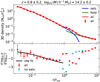 |
Fig. 52 Galaxy distribution as a function of halo radius. Top: galaxy density profile as a function of halo-centric distance, showing the combined halo galaxy density profile and its transition into the field. We select 420 haloes with the same criteria as in Fig. 17 (0.6 < ɀ < 1.0 and 14.0 < log10[M/(h−1 M⊙)] < 14.4). The density for all galaxies is marked with red dots, whose error bars are small and hard to distinguish, and joined with a solid red line. The density for the satellites belonging to the halo (which are placed out to 3 rvir) are in blue and in green is the density of galaxies in the field (outside the halo). Bottom: slope of the galaxy density profile for all galaxies (red points with error bars) and the value of the slope of the NFW profile that best fits the density profile of all galaxies out to the virial radius. The cyan dots show the slope that we would get if we did not take into account the satellites of the haloes beyond the virial radius. In this case the splashback radius is clearly visible slightly beyond the virial radius. Both panels show that in the region between 1 and 3 virial radii we are overpopulating with galaxies. |
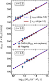 |
Fig. 53 Halo line-of-sight velocity dispersion vs. halo mass, for lightcones from the GAEA semi-analytical model (without orphan galaxies, blue circles, 7 deg2) and for Flagship (red stars, here for the 49 deg2 region), at three representative redshifts. The lines are simple non-theoretical representations. While Flagship uses virial quantities, GAEA uses R200c for the virial radius and therefore the x axis is log10[M200c/(h−1 M⊙)] for GAEA. Only haloes with at least 10 member galaxies with IE < 24.5 and HE < 24 within the virial cylinder are considered, with at least 10 such haloes per mass bin. The velocity dispersions are measured with the gapper method (Wainer & Thissen 1976), and the error bars assume Gaussian velocity distributions, i.e., |

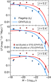 |
Fig. 54 Cluster luminosity functions of red and blue color_kind galaxies for Flagship (points) together with Schechter (1976) functions fit to early-type (ETG) and late-type (LTG) galaxies by Sarron et al. (2018) as a function of the CFHTLS absolute magnitudes (lines). The samples were selected to have IE < 23 (Flagship) and i < 23 (CFHTLS). The normalisation for both CFHTLS and Flagship is per cylinder of 1 h−1 Mpc radius, where the cylinder is very long for CFHTLS, given the uncertainties in the photometric redshifts, while it is limited to 1.5 rvir for Flagship. The abscissae of the points are slightly offset for clarity. The discrepancies between the CFHTLS analysis and Flagship are discussed in the text. |
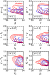 |
Fig. 55 Contours of the colour-magnitude diagrams of Flagship field galaxies (blue) and cluster (Mvir > 1014 h−1 M⊙) galaxies (red), at selected redshifts. The figure uses proxies for the rest-frame U − B and rest-frame B magnitude. The galaxies are limited to IE < 24.5 and HE < 24. The redshift bins have widths of ±0.05,0.06,0.07,0.1,0.2, and 0.2. The contours are spaced by 0.2 dex and are KDE-smoothed. The figure highlights how the Red Sequence is more prominent in clusters. |
8 Future developments
Modelling the properties of a massive and complex galaxy survey such as Euclid necessarily entails making certain assumptions and approximations with respect to the true galaxy samples. Below we discuss some of the possible shortcomings in the approach we have taken in the modelling, how they can impact the different observables and, in some cases, how these could be improved in future releases of the Flagship galaxy mock.
In this paper we have implemented a simple HOD approach to assign galaxies to dark-matter haloes, in which the number of satellite galaxies in each halo depend only on the halo mass. Several studies have shown that other halo properties are needed to accurately simulate the galaxy population within this type of framework. This is commonly referred to as halo assembly bias (e.g., Contreras et al. 2023). While our HOD prescription is simple, the way we assign galaxy properties is more complex than the approach of typical HOD and AM models, and in a certain sense our method resembles models that introduce assembly bias as our galaxy properties assignment depends on other parameters. For example, the way we distribute galaxies within haloes depends on galaxy colour which can be related to the assembly history (e.g., Hearin & Watson 2013). Moreover, normally observations of a particular galaxy sample, selected with a flux limit or colour criteria as for example luminous red galaxies, are interpreted in the HOD framework fitting parameters of the occupancy distribution. In the Flagship catalogue, the HOD is assigned up front and corresponds to the whole population. Any galaxy subsample selected with colour and/or flux cuts will have a different HOD than the original assignment. Similarly, we have not included the effects of gas physics, which are expected to significantly alter the distribution of dark matter and thus of galaxies within galaxy cluster scales (e.g., Schneider & Teyssier 2015; Gebhardt et al. 2024). Again, our galaxy properties assignment depends on luminosity and colour in order to fit observations, and therefore it must incorporate the effect that baryons have on the galaxy distributions when compared to dark-matter only simulations. Nevertheless, we are exploring HOD prescriptions that depend on other parameters for implementation in future versions of the catalogue.
Another improvement in the catalogue that we are considering is to increase the resolution of the HEALPix lensing maps. Currently, we use a pixel scale of 0’43, i.e., HEALPix Nside = 8192, without interpolation between pixels. This resolution is enough to measure adequately the lensing correlation functions down to 1 arcmin (e.g., for ξ+ and the tangential shear), which coincide with the smallest scales probed by Euclid. Therefore, the resolution of the lensing properties is good enough for the main purpose of the simulation. Moreover, in the MICE-Grand Challenge simulation (Fosalba et al. 2015), which used the same assignment scheme, we tested that interpolating linearly between the HEALPix pixels only improved marginally the effective resolution on sub-arcmin scales, and at a high computational cost.
We are also exploring how to improve our SED assignment. Currently, we use linear interpolation between SEDs selected from the COSMOS SED template set (see Sect. 5.4). We would like to use a wider set of templates that can cover better the range of observed SEDs as a function of redshift. We are also investigating using a wider wavelength range to assign SEDs instead of using a single colour, which has led to selecting templates that are too bright in the near-infrared. Another shortcoming of our simulation is the lack of AGN. We are working on methods to include them in future versions (e.g., Allevato et al. 2021).
The calibration of our recipes to assign galaxy properties are normally restricted to low-redshift observed samples, ɀ ≲ 1, which we extrapolate to higher redshifts. We are working on extending the calibration to higher redshifts using more observational data.
The assignment of galaxy positions and velocities is simplistic, relying on analytic profiles without substructure. This is mainly driven by our push to simulate faint galaxies while covering a large volume. While for the relevant scales to be explored with the Euclid main cosmological probes this level of detail is enough, we are exploring keeping more information from the original N -body simulation to be able to produce more realistic galaxy profiles within haloes and therefore support more extensive cluster science analyses. In particular, the approach used to extend satellite galaxies beyond the virial radius is producing spurious density profile features in the outskirts of haloes. We will correct this procedure in future versions of the catalogue.
We have assigned shapes and sizes to galaxies based on distributions measured with HST. The distributions of each parameter are well reproduced by our catalogue. However, we have not enforced the correlations between different morphological parameters in part due to the usage of two different samples for our calibration. We are working on a multi-parameter calibration for future implementations, that will be based on the Euclid data themselves which are going to provide a large and homogeneously measured morphological sample.
Data availability
Given the comprehensive set of validation tests that we have performed on the Flagship galaxy mock catalogue, we believe it is a valuable resource to perform a wide suite of astrophysical analyses beyond its original design goals of supporting the Euclid weak lensing and galaxy clustering analyses. We make the catalogue publicly available so that everybody can potentially benefit from its usage. We distribute this catalogue from the CosmoHub platform.
Acknowledgements
FJC and PF acknowledge support form the Spanish Min- isterio de Ciencia, Innovación y Universidades, projects PID2019-11317GB, PID2022-141079NB, PID2022-138896NB; the European Research Executive Agency HORIZON-MSCA-2021-SE-01 Research and Innovation programme under the Marie Skłodowska-Curie grant agreement number 101086388 (LACE- GAL) and the programme Unidad de Excelencia María de Maeztu, project CEX2020-001058-M. We acknowledge the support of the PRACE project (Call 17) “Simulating the Euclid Universe” for the computer time on the Piz Daint supercomputer at CSCS, Lugano, Switzerland, which made possible the worldleading Flagship 2 N-body simulation. The Port d’Informació Científica (PIC) is maintained through a collaboration between CIEMAT and IFAE. This work has been supported by MCIN/AEI grant EQC2021-007479-P and European Union NextGenerationEU grant PRTR-C17.I1 and by Generalitat de Catalunya. This work has been partially funded by Premiale MITIC 2015. The Euclid Consortium acknowledges the European Space Agency and a number of agencies and institutes that have supported the development of Euclid, in particular the Agenzia Spaziale Italiana, the Austrian Forschungsförderungsgesellschaft funded through BMK, the Belgian Science Policy, the Canadian Euclid Consortium, the Deutsches Zentrum für Luft- und Raumfahrt, the DTU Space and the Niels Bohr Institute in Denmark, the French Centre National d’Etudes Spatiales, the Fundação para a Ciência e a Tecnologia, the Hungarian Academy of Sciences, the Ministerio de Ciencia, Innovación y Universidades, the National Aeronautics and Space Administration, the National Astronomical Observatory of Japan, the Netherlandse Onderzoekschool Voor Astronomie, the Norwegian Space Agency, the Research Council of Finland, the Romanian Space Agency, the State Secretariat for Education, Research, and Innovation (SERI) at the Swiss Space Office (SSO), and the United Kingdom Space Agency. A complete and detailed list is available on the Euclid web site (https://www.euclid-ec.org).
Appendix A Halo mass function with different mass estimates
The Flagship halo catalogue was produced with the ROCKSTAR code adapted to the lightcone (see Sect. 4). ROCKSTAR computes different estimates of the halo mass. The mass values that we calculated are the mass of the particles linked together with a friends-of-friends algorithm of linking length b = 0.2, Mfof; the mass contained within the virial radius, Mvir; the sum of the mass of the bound particles within the virial radius, Mbound; the mass of the particles within an overdensity of 200 relative to the background density, M200b; and the mass of the particles within an overdensity of 200 relative to the critical density, M200c.
In this Appendix, we provide a comparison of the cumulative halo mass function resulting from the different mass estimates and also to the T08 Mvir halo mass function as a function of redshift.
Figure A.1 shows the ratio of the cumulative halo mass function for all the mass estimates to the cumulative Mbound HMF. It also contains the ratio of the T08 Mbound HMF to the Mbound HMF for comparison. The Mvir and Mbound HMFs coincide except for small differences at the low and high-mass end due to the unbound particle rejection process. The M200b HMF is higher than the Mbound HMF at low redshift ɀ < 1, similar at 1.0 < ɀ < 1.5, and lower at ɀ > 1.5. The M200c HMF is always lower than the Mbound HMF. The M200b and M200c HMFs vary as expected due to the different redshift dependence of the density threshold used to define the mass. The ratio of the background density to the critical density gets lower at low redshift when the effect of ΩΛ starts to be important, therefore increasing the ratio of M200b to the M200c values. The Mfof HMF is quite different from the Mbound HMF. This is expected as the friends-of-friends halo-finding technique and its mass definition is different from the rest. The T08 Mvir HMF shows the same trends as described in Sect. 4.1.
Appendix B The SciPic algorithm
SciPIC, first described in Carretero et al. (2017) and named after Scientific Pipeline at PIC, is a suite of algorithms integrated into a powerful pipeline dedicated to the generation of massive synthetic galaxy catalogues based on halo catalogues coming from N-body dark matter cosmological simulations. SciPIC is the algorithm used to generate the Euclid Flagship galaxies. Originally, most of the algorithms were developed to the production of the MICE galaxy catalogues. In the case of MICE, the code was written in C and executed on different desktops. In particular, a significant amount of time was dedicated to input-output tasks, given that several steps were executed sequentially. However, with the Flagship parent halo catalogue containing a much larger volume of data, the methodology employed for running the MICE catalogue is unfeasible. The code has been refactored, optimised, and ported to Python. Additionally, it runs on top of Apache Spark, an engine for scaleable computing. SciPIC is executed in the PIC Big Data platform, based on Hadoop, which comprises 20 nodes for a total processing power of 960 CPUs. The code runs efficiently with a fast interface with the Cosmo-Hub portal (Tallada et al. 2020), where the input halo catalogue is ingested, and the output galaxy catalogues are stored and distributed. The current implementation is able to generate a 15TB catalogue of 5B galaxies in 3 hours. The fact that it takes so little time to generate a mock allows for multiple iterations of progressive refinement.
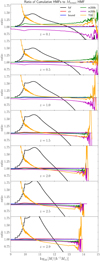 |
Fig. A.1 Ratio of the cumulative halo mass function for all mass estimates computed with ROCKSTAR and also the T08 Mvir HMF to the Mbound cumulative HMF as a function of redshift. |
Appendix C Details of the measurement of radial velocity dispersions of galaxies in their haloes
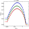 |
Fig. C.1 Adopted model for the radial velocity dispersion profiles in virial units, for the case of dark matter concentration of 4, for the three galaxy classes. The symbols indicate the exact values, while the curves indicate the 2D-fifth-order polynomial approximations used in the Flagship. One clearly sees the adopted constant values beyond the fit limits of r/rvir. |
We provide here details on the mock velocities. The Jeans equation (14) is solved for the dynamical pressure,  , which for the Tiret et al. (2007) velocity anisotropy profile of Eq. (15) is (Mamon et al. 2013)
 (C.1)
(C.1)
trivially yielding the radial velocity dispersion σr for our chosen NFW model for ρ(r). For each of the three galaxy colour classes, we pre-computed σr using Eq. (C.1) on a 25x16 grid of [log10(r/rvir),log10(cdark)], with −2 ≤ log10(r/rvir) ≤ 0.4 and −1 ≤ log10(cdark) ≤ 1.5, in steps of 0.1 dex. We then fit a two-dimensional 5th-order polynomial to allow Flagship to rapidly determine the radial velocity dispersion at given radial distances. The rms errors on log10 σr are 0.0019, 0.0022, and 0.0026 respectively for red, green, and blue galaxies, i.e., better than 0.6% rms precision on σr for all colour classes.
Appendix D SED assignment example
In order to clarify the procedure followed to assign SEDs to galaxies described in Sect. 5.4, we present here a step-by-step walk-through example. Let us start with a galaxy with a colour of (ɡ01 − r01)HOD = 0.35, located at redshift ɀ = 1.45. We are going to find two templates, SED(ɀ1) and SED(ɀ2), from the COSMOS set at redshifts ɀ1 = 1.0 and ɀ2 = 1.5, which we are going to combine linearly as in Eq. (17), with weights w1 =0.1 and w2 = 0.9 (Eq. (18)).
In Table D.l we provide the values obtained for the quantities computed in this process, which we are going to describe below. We find the COSMOS ɡ − r colour that corresponds to (ɡ01 − r01)HOD = 0.35 at redshifts ɀ1 and ɀ2. These are ɡ − r = 0.084 and ɡ − r = −0.008, respectively (4th column in Table D.1). These colours correspond to the ordered template indexes  and
and  at their redshifts, respectively. We choose the six ordered templates that have ɡ − r colours closer to the ones computed before (5th column of the table). These ordered templates are defined as a tuple of three numbers: the SED index of our COSMOS template library (Ilbert et al. 2009, see Sect. 5.4); the extinction law (0 = None, 1=Prévot, 2 = Calzetti); and the E(B − V) value (6th column of the table). We compute the ɡ − r colour difference between these ordered templates and the reference colour (7th column), and assign a probability to that colour difference (PCol, 8th column), taking into account the six ordered templates (see Sect. 5.4 for details). We normalise these colour probabilities so that the sum of the probabilities of the six ordered templates is one, i.e.,
  , where the index i runs through the six ordered templates. We multiply the colour probabilities by the E(B − V) probabilities (PE(b−v), 9th column), shown in Fig. 19 to obtain the total probability (Ptot, 10th column). The normalisation of the E(B − V) probabilities is such that the sum of the probabilities for all the values of E(B − V) at a given reference redshift is one, i.e.,
  , where the index j runs through all the E(B − V) values. The total probability, Ptot, is normalised such that the sum of the probabilities of the six ordered templates is one, i.e.,
  where the index i runs through the six ordered templates.
Finally we draw a random number from a uniform distribution in the range [0,1] and assign the ordered template (11th column of Table D.l) based on this random number and the total probability of each ordered template, which corresponds to the final SED given in the 12th column of the table. We note that the ordered template with the highest Ptot is not necessarily the one chosen, as is the case for the first one in this example. The final SED for this galaxy is the linear combination of these two templates, applying Eqs. (17) and (18), with the weights, w1 =0.1 and w2 = 0.9, mentioned before.
SED assignment step values for a galaxy at z = 1.45 and colour (ɡ01 − r01)HOD = 0.35.
References
- Abbott, T. M. C., Aguena, M., Alarcon, A., et al. 2023, Phys. Rev. D, 107, 083504 [NASA ADS] [CrossRef] [Google Scholar]
- Adhikari, S., Dalal, N., & Chamberlain, R. T. 2014, J. Cosmology Astropart. Phys., 2014, 019 [CrossRef] [Google Scholar]
- Aihara, H., Armstrong, R., Bickerton, S., et al. 2018, PASJ, 70, S8 [NASA ADS] [Google Scholar]
- Akeson, R., Armus, L., Bachelet, E., et al. 2019, arXiv e-prints [arXiv:1902.05569] [Google Scholar]
- Albrecht, A., Bernstein, G., Cahn, R., et al. 2006, arXiv e-prints [arXiv:astro-ph/0609591] [Google Scholar]
- Allevato, V., Shankar, F., Marsden, C., et al. 2021, ApJ, 916, 34 [NASA ADS] [CrossRef] [Google Scholar]
- Amendola, L., Appleby, S., Avgoustidis, A., et al. 2018, Liv. Rev. Relativ., 21, 2 [NASA ADS] [CrossRef] [Google Scholar]
- Angulo, R. E., & Hahn, O. 2022, Liv. Rev. Computat. Astrophys., 8, 1 [CrossRef] [Google Scholar]
- Angulo, R. E., Zennaro, M., Contreras, S., et al. 2021, MNRAS, 507, 5869 [NASA ADS] [CrossRef] [Google Scholar]
- Bagley, M. B., Scarlata, C., Mehta, V., et al. 2020, ApJ, 897, 98 [NASA ADS] [CrossRef] [Google Scholar]
- Balaguera-Antolínez, A., Kitaura, F.-S., Alam, S., et al. 2023, A&A, 673, A130 [NASA ADS] [CrossRef] [EDP Sciences] [Google Scholar]
- Baldry, I. K., Balogh, M. L., Bower, R., Glazebrook, K., & Nichol, R. C. 2004, in American Institute of Physics Conference Series, 743, The New Cosmology: Conference on Strings and Cosmology, eds. R. E. Allen, D. V. Nanopoulos, & C. N. Pope, 106 [Google Scholar]
- Baldwin, J. A., Phillips, M. M., & Terlevich, R. 1981, PASP, 93, 5 [Google Scholar]
- Bartelmann, M., & Schneider, P. 2001, Phys. Rep., 340, 291 [Google Scholar]
- Behroozi, P. S., Conroy, C., & Wechsler, R. H. 2010, ApJ, 717, 379 [Google Scholar]
- Behroozi, P. S., Wechsler, R. H., & Wu, H.-Y. 2013, ApJ, 762, 109 [NASA ADS] [CrossRef] [Google Scholar]
- Behroozi, P., Wechsler, R. H., Hearin, A. P., & Conroy, C. 2019, MNRAS, 488, 3143 [NASA ADS] [CrossRef] [Google Scholar]
- Benson, A. J., Cole, S., Frenk, C. S., Baugh, C. M., & Lacey, C. G. 2000, MNRAS, 311, 793 [NASA ADS] [CrossRef] [Google Scholar]
- Berlind, A. A., & Weinberg, D. H. 2002, ApJ, 575, 587 [Google Scholar]
- Bertschinger, E., & Gelb, J. M. 1991, Comput. Phys., 5, 164 [NASA ADS] [CrossRef] [Google Scholar]
- Bianchi, D., Gil-Marín, H., Ruggeri, R., & Percival, W. J. 2015, MNRAS, 453, L11 [NASA ADS] [CrossRef] [Google Scholar]
- Blanton, M. R., Hogg, D. W., Bahcall, N. A., et al. 2003, ApJ, 592, 819 [Google Scholar]
- Blanton, M. R., Lupton, R. H., Schlegel, D. J., et al. 2005a, ApJ, 631, 208 [Google Scholar]
- Blanton, M. R., Schlegel, D. J., Strauss, M. A., et al. 2005b, AJ, 129, 2562 [NASA ADS] [CrossRef] [Google Scholar]
- Breton, M.-A., de la Torre, S., & Piat, J. 2022, A&A, 661, A154 [NASA ADS] [CrossRef] [EDP Sciences] [Google Scholar]
- Bruzual, G., & Charlot, S. 2003, MNRAS, 344, 1000 [NASA ADS] [CrossRef] [Google Scholar]
- Bryan, G. L., & Norman, M. L. 1998, ApJ, 495, 80 [NASA ADS] [CrossRef] [Google Scholar]
- Buchner, J., Georgakakis, A., Nandra, K., et al. 2014, A&A, 564, A125 [NASA ADS] [CrossRef] [EDP Sciences] [Google Scholar]
- Bullock, J. S., Wechsler, R. H., & Somerville, R. S. 2002, MNRAS, 329, 246 [Google Scholar]
- Butcher, H., & Oemler, A., J. 1978, ApJ, 219, 18 [NASA ADS] [CrossRef] [Google Scholar]
- Calzetti, D., Armus, L., Bohlin, R. C., et al. 2000, ApJ, 533, 682 [NASA ADS] [CrossRef] [Google Scholar]
- Carretero, J., Castander, F. J., Gaztañaga, E., Crocce, M., & Fosalba, P. 2015, MNRAS, 447, 646 [NASA ADS] [CrossRef] [Google Scholar]
- Carretero, J., Tallada, P., Casals, J., et al. 2017, in Proceedings of the European Physical Society Conference on High Energy Physics, 5-12 July, 488 [Google Scholar]
- Chabrier, G. 2003, PASP, 115, 763 [Google Scholar]
- Chon, G., Challinor, A., Prunet, S., Hivon, E., & Szapudi, I. 2004, MNRAS, 350, 914 [Google Scholar]
- Cole, S., Lacey, C. G., Baugh, C. M., & Frenk, C. S. 2000, MNRAS, 319, 168 [Google Scholar]
- Collister, A. A., & Lahav, O. 2005, MNRAS, 361, 415 [Google Scholar]
- Comparat, J., Prada, F., Yepes, G., & Klypin, A. 2017, MNRAS, 469, 4157 [NASA ADS] [CrossRef] [Google Scholar]
- Contreras, S., Angulo, R. E., Chaves-Montero, J., White, S. D. M., & Aricò, G. 2023, MNRAS, 520, 489 [Google Scholar]
- Cooray, A., & Sheth, R. 2002, Phys. Rep., 372, 1 [Google Scholar]
- Couchman, H. M. P., Thomas, P. A., & Pearce, F. R. 1995, ApJ, 452, 797 [NASA ADS] [CrossRef] [Google Scholar]
- Crittenden, R. G., Natarajan, P., Pen, U.-L., & Theuns, T. 2002, ApJ, 568, 20 [NASA ADS] [CrossRef] [Google Scholar]
- Curti, M., Mannucci, F., Cresci, G., & Maiolino, R. 2020, MNRAS, 491, 944 [Google Scholar]
- Dahlen, T., Mobasher, B., Somerville, R. S., et al. 2005, ApJ, 631, 126 [Google Scholar]
- Dakin, J., Hannestad, S., & Tram, T. 2022, MNRAS, 513, 991 [CrossRef] [Google Scholar]
- d’Amico, G., Gleyzes, J., Kokron, N., et al. 2020, J. Cosmology Astropart. Phys., 5, 005 [Google Scholar]
- De Lucia, G., Fontanot, F., Xie, L., & Hirschmann, M. 2024, A&A, 687, A68 [NASA ADS] [CrossRef] [EDP Sciences] [Google Scholar]
- de Putter, R., & Takada, M. 2010, Phys. Rev. D, 82, 103522 [Google Scholar]
- de Salas, P. F., Forero, D. V., Ternes, C. A., Tórtola, M., & Valle, J. W. F. 2018, Phys. Lett. B, 782, 633 [Google Scholar]
- Despali, G., Giocoli, C., Angulo, R. E., et al. 2016, MNRAS, 456, 2486 [NASA ADS] [CrossRef] [Google Scholar]
- Dey, A., Schlegel, D. J., Lang, D., et al. 2019, AJ, 157, 168 [Google Scholar]
- Diemer, B. 2018, ApJS, 239, 35 [NASA ADS] [CrossRef] [Google Scholar]
- Diemer, B., & Kravtsov, A. V. 2014, ApJ, 789, 1 [NASA ADS] [CrossRef] [Google Scholar]
- Diemer, B., & Joyce, M. 2019, ApJ, 871, 168 [NASA ADS] [CrossRef] [Google Scholar]
- Dimauro, P., Huertas-Company, M., Daddi, E., et al. 2018, MNRAS, 478, 5410 [Google Scholar]
- Dolag, K., Komatsu, E., & Sunyaev, R. 2016, MNRAS, 463, 1797 [Google Scholar]
- Dong-Páez, C. A., Smith, A., Szewciw, A. O., et al. 2024, MNRAS, 528, 7236 [CrossRef] [Google Scholar]
- Driver, S. P., Andrews, S. K., Davies, L. J., et al. 2016, ApJ, 827, 108 [CrossRef] [Google Scholar]
- Driver, S. P., Bellstedt, S., Robotham, A. S. G., et al. 2022, MNRAS, 513, 439 [NASA ADS] [CrossRef] [Google Scholar]
- Dubois, Y., Pichon, C., Welker, C., et al. 2014, MNRAS, 444, 1453 [Google Scholar]
- Eggemeier, A., Camacho-Quevedo, B., Pezzotta, A., et al. 2023, MNRAS, 519, 2962 [Google Scholar]
- Ereza, J., Prada, F., Klypin, A., et al. 2024, MNRAS, 532, 1659 [NASA ADS] [CrossRef] [Google Scholar]
- Euclid Collaboration (Blanchard, A., et al.) 2020, A&A, 642, A191 [NASA ADS] [CrossRef] [EDP Sciences] [Google Scholar]
- Euclid Collaboration (Knabenhans, M., et al.) 2021, MNRAS, 505, 2840 [NASA ADS] [CrossRef] [Google Scholar]
- Euclid Collaboration (Scaramella, R., et al.) 2022, A&A, 662, A112 [NASA ADS] [CrossRef] [EDP Sciences] [Google Scholar]
- Euclid Collaboration (Jelic-Cizmek, G., et al.) 2024, A&A, 685, A167 [NASA ADS] [CrossRef] [EDP Sciences] [Google Scholar]
- Euclid Collaboration (Serrano, S., et al.) 2024, A&A, 690, A103 [NASA ADS] [CrossRef] [EDP Sciences] [Google Scholar]
- Euclid Collaboration (Enia, A., et al.) 2024, A&A, 691, A175 [NASA ADS] [Google Scholar]
- Euclid Collaboration (Cropper, M. S., et al.) 2025, A&A, 697, A2 (Euclid on Sky SI) [Google Scholar]
- Euclid Collaboration (Jahnke, K., et al.) 2025, A&A, 697, A3 (Euclid on Sky SI) [Google Scholar]
- Euclid Collaboration (Mellier, Y., et al.) 2025, A&A, 697, A1 (Euclid on Sky SI) [Google Scholar]
- Fidler, C., Kleinjohann, A., Tram, T., Rampf, C., & Koyama, K. 2019, J. Cosmology Astropart. Phys., 01, 025 [Google Scholar]
- Fosalba, P., & Szapudi, I. 2004, ApJ, 617, L95 [Google Scholar]
- Fosalba, P., Gaztañaga, E., Castander, F. J., & Manera, M. 2008, MNRAS, 391, 435 [NASA ADS] [CrossRef] [Google Scholar]
- Fosalba, P., Gaztañaga, E., Castander, F. J., & Crocce, M. 2015, MNRAS, 447, 1319 [NASA ADS] [CrossRef] [Google Scholar]
- Garrison, L. H., Eisenstein, D. J., & Pinto, P. A. 2019, MNRAS, 485, 3370 [CrossRef] [Google Scholar]
- Garrison, L. H., Eisenstein, D. J., Ferrer, D., Maksimova, N. A., & Pinto, P. A. 2021, MNRAS, 508, 575 [NASA ADS] [CrossRef] [Google Scholar]
- Gebhardt, M., Anglés-Alcázar, D., Borrow, J., et al. 2024, MNRAS, 529, 4896 [NASA ADS] [CrossRef] [Google Scholar]
- Giavalisco, M., Ferguson, H. C., Koekemoer, A. M., et al. 2004, ApJ, 600, L93 [NASA ADS] [CrossRef] [Google Scholar]
- Ginzburg, D., Desjacques, V., & Chan, K. C. 2017, Phys. Rev. D, 96, 083528 [NASA ADS] [CrossRef] [Google Scholar]
- Górski, K. M., Hivon, E., Banday, A. J., et al. 2005, ApJ, 622, 759 [Google Scholar]
- Grieb, J. N., Sánchez, A. G., Salazar-Albornoz, S., & Dalla Vecchia, C. 2016, MNRAS, 457, 1577 [NASA ADS] [CrossRef] [Google Scholar]
- Grogin, N. A., Kocevski, D. D., Faber, S. M., et al. 2011, ApJS, 197, 35 [NASA ADS] [CrossRef] [Google Scholar]
- Gu, Y., Yang, X., Han, J., et al. 2024, MNRAS, 529, 4015 [NASA ADS] [CrossRef] [Google Scholar]
- Habib, S., Pope, A., Finkel, H., et al. 2016, New A, 42, 49 [Google Scholar]
- Harnois-Déraps, J., Pen, U.-L., Iliev, I. T., et al. 2013, MNRAS, 436, 540 [Google Scholar]
- Hatton, S., Devriendt, J. E. G., Ninin, S., et al. 2003, MNRAS, 343, 75 [Google Scholar]
- Hearin, A. P., & Watson, D. F. 2013, MNRAS, 435, 1313 [Google Scholar]
- Heydenreich, S., Linke, L., Burger, P., & Schneider, P. 2023, A&A, 672, A44 [NASA ADS] [CrossRef] [EDP Sciences] [Google Scholar]
- Heymans, C., Tröster, T., Asgari, M., et al. 2021, A&A, 646, A140 [NASA ADS] [CrossRef] [EDP Sciences] [Google Scholar]
- Hilbert, S., Hartlap, J., White, S. D. M., & Schneider, P. 2009, A&A, 499, 31 [NASA ADS] [CrossRef] [EDP Sciences] [Google Scholar]
- Hilbert, S., Barreira, A., Fabbian, G., et al. 2020, MNRAS, 493, 305 [Google Scholar]
- Hirschmann, M., De Lucia, G., & Fontanot, F. 2016, MNRAS, 461, 1760 [Google Scholar]
- Hu, W. 2000, Phys. Rev. D, 62, 043007 [NASA ADS] [CrossRef] [Google Scholar]
- Ilbert, O., Arnouts, S., McCracken, H. J., et al. 2006, A&A, 457, 841 [NASA ADS] [CrossRef] [EDP Sciences] [Google Scholar]
- Ilbert, O., Capak, P., Salvato, M., et al. 2009, ApJ, 690, 1236 [NASA ADS] [CrossRef] [Google Scholar]
- Ilbert, O., McCracken, H. J., Le Fèvre, O., et al. 2013, A&A, 556, A55 [NASA ADS] [CrossRef] [EDP Sciences] [Google Scholar]
- Ishiyama, T., Prada, F., Klypin, A. A., et al. 2021, MNRAS, 506, 4210 [NASA ADS] [CrossRef] [Google Scholar]
- Ivanov, M. M., Simonović, M., & Zaldarriaga, M. 2020, J. Cosmology Astropart. Phys., 05, 042 [Google Scholar]
- Ivezić, Ž., Kahn, S. M., Tyson, J. A., et al. 2019, ApJ, 873, 111 [Google Scholar]
- Jarvis, M., Bernstein, G., & Jain, B. 2004, MNRAS, 352, 338 [Google Scholar]
- Jelic-Cizmek, G., Lepori, F., Bonvin, C., & Durrer, R. 2021, J. Cosmology Astropart. Phys., 4, 055 [Google Scholar]
- Jeong, D., Komatsu, E., & Jain, B. 2009, Phys. Rev. D, 80, 123527 [Google Scholar]
- Jing, Y. P., Mo, H. J., & Boerner, G. 1998, ApJ, 494, 1 [NASA ADS] [CrossRef] [Google Scholar]
- Johnston, H., Georgiou, C., Joachimi, B., et al. 2019, A&A, 624, A30 [NASA ADS] [CrossRef] [EDP Sciences] [Google Scholar]
- Juneau, S., Bournaud, F., Charlot, S., et al. 2014, ApJ, 788, 88 [NASA ADS] [CrossRef] [Google Scholar]
- Kashino, D., Silverman, J. D., Sanders, D., et al. 2019, ApJS, 241, 10 [Google Scholar]
- Kauffmann, G., White, S. D. M., & Guiderdoni, B. 1993, MNRAS, 264, 201 [Google Scholar]
- Kauffmann, G., Colberg, J. M., Diaferio, A., & White, S. D. M. 1999, MNRAS, 303, 188 [NASA ADS] [CrossRef] [Google Scholar]
- Kennicutt, R. C. Jr., 1998, ARA&A, 36, 189 [NASA ADS] [CrossRef] [Google Scholar]
- Kewley, L. J., Dopita, M. A., Leitherer, C., et al. 2013a, ApJ, 774, 100 [NASA ADS] [CrossRef] [Google Scholar]
- Kewley, L. J., Maier, C., Yabe, K., et al. 2013b, ApJ, 774, L10 [Google Scholar]
- Kilbinger, M., Bonnett, C., & Coupon, J. 2014, athena: Tree code for second- order correlation functions, Astrophysics Source Code Library [record ascl:1402.026] [Google Scholar]
- Klypin, A., & Prada, F. 2018, MNRAS, 478, 4602 [NASA ADS] [CrossRef] [Google Scholar]
- Klypin, A., Gottlöber, S., Kravtsov, A. V., & Khokhlov, A. M. 1999, ApJ, 516, 530 [NASA ADS] [CrossRef] [Google Scholar]
- Koekemoer, A. M., Faber, S. M., Ferguson, H. C., et al. 2011, ApJS, 197, 36 [NASA ADS] [CrossRef] [Google Scholar]
- Kovacs, E., Mao, Y.-Y., Aguena, M., et al. 2022, Open J. Astrophys., 5, 1 [NASA ADS] [CrossRef] [Google Scholar]
- Kravtsov, A. V., Berlind, A. A., Wechsler, R. H., et al. 2004, ApJ, 609, 35 [Google Scholar]
- Kriek, M., Shapley, A. E., Reddy, N. A., et al. 2015, ApJS, 218, 15 [NASA ADS] [CrossRef] [Google Scholar]
- Lagos, C. D. P., Tobar, R. J., Robotham, A. S. G., et al. 2018, MNRAS, 481, 3573 [CrossRef] [Google Scholar]
- Landy, S. D., & Szalay, A. S. 1993, ApJ, 412, 64 [Google Scholar]
- Laureijs, R., Amiaux, J., Arduini, S., et al. 2011, arXiv e-prints [arXiv:1110.3193] [Google Scholar]
- Lesgourgues, J. 2011, arXiv e-prints [arXiv:1104.2932] [Google Scholar]
- Lewis, A. 2005, Phys. Rev. D, 71, 083008 [Google Scholar]
- Lewis, A., Challinor, A., & Lasenby, A. 2000, ApJ, 538, 473 [Google Scholar]
- LoVerde, M., & Afshordi, N. 2008, Phys. Rev. D, 78, 123506 [NASA ADS] [CrossRef] [Google Scholar]
- LSST Dark Energy Science Collaboration (LSST DESC) (Abolfathi, B., et al.) 2021, ApJS, 253, 31 [CrossRef] [Google Scholar]
- Mahajan, S., Mamon, G. A., & Raychaudhury, S. 2011, MNRAS, 416, 2882 [NASA ADS] [CrossRef] [Google Scholar]
- Mamon, G. A., Biviano, A., & Boué, G. 2013, MNRAS, 429, 3079 [Google Scholar]
- Mamon, G. A., Cava, A., Biviano, A., et al. 2019, A&A, 631, A131 [NASA ADS] [CrossRef] [EDP Sciences] [Google Scholar]
- Mannucci, F., Belfiore, F., Curti, M., et al. 2021, MNRAS, 508, 1582 [NASA ADS] [CrossRef] [Google Scholar]
- McDonough, B., & Brainerd, T. G. 2022, ApJ, 933, 161 [Google Scholar]
- Mead, A. J., Brieden, S., Tröster, T., & Heymans, C. 2021, MNRAS, 502, 1401 [Google Scholar]
- Menon, H., Wesolowski, L., Zheng, G., et al. 2015, Computat. Astrophys. Cosmol., 2, 1 [Google Scholar]
- Merson, A., Smith, A., Benson, A., Wang, Y., & Baugh, C. 2019, MNRAS, 486, 5737 [Google Scholar]
- Miller, L., Heymans, C., Kitching, T. D., et al. 2013, MNRAS, 429, 2858 [Google Scholar]
- Moessner, R., & Jain, B. 1998, MNRAS, 294, L18 [Google Scholar]
- More, S., van den Bosch, F. C., & Cacciato, M. 2009, MNRAS, 392, 917 [Google Scholar]
- Moretti, C., Tsedrik, M., Carrilho, P., & Pourtsidou, A. 2023, J. Cosmology Astropart. Phys., 12, 025 [Google Scholar]
- Moster, B. P., Somerville, R. S., Maulbetsch, C., et al. 2010, ApJ, 710, 903 [Google Scholar]
- Moster, B. P., Naab, T., & White, S. D. M. 2018, MNRAS, 477, 1822 [Google Scholar]
- Murray, S. G., Power, C., & Robotham, A. S. G. 2013, Astron. Comput., 3, 23 [CrossRef] [Google Scholar]
- Navarro, J. F., Frenk, C. S., & White, S. D. M. 1997, ApJ, 490, 493 [Google Scholar]
- O’Neil, S., Barnes, D. J., Vogelsberger, M., & Diemer, B. 2021, MNRAS, 504, 4649 [CrossRef] [Google Scholar]
- Osterbrock, D., & Ferland, G. 2006, Astrophysics Of Gas Nebulae and Active Galactic Nuclei (University Science Books) [Google Scholar]
- Peacock, J. A., & Smith, R. E. 2000, MNRAS, 318, 1144 [Google Scholar]
- Pillepich, A., Springel, V., Nelson, D., et al. 2018, MNRAS, 473, 4077 [Google Scholar]
- Planck Collaboration VI. 2020, A&A, 641, A6 [NASA ADS] [CrossRef] [EDP Sciences] [Google Scholar]
- Polletta, M., Tajer, M., Maraschi, L., et al. 2007, ApJ, 663, 81 [NASA ADS] [CrossRef] [Google Scholar]
- Potter, D., & Stadel, J. 2016, PKDGRAV3: Parallel gravity code, Astrophysics Source Code Library [record ascl:1609.016] [Google Scholar]
- Potter, D., Stadel, J., & Teyssier, R. 2017, Computat. Astrophys. Cosmol., 4, 2 [NASA ADS] [CrossRef] [Google Scholar]
- Pozzetti, L., Hirata, C. M., Geach, J. E., et al. 2016, A&A, 590, A3 [NASA ADS] [CrossRef] [EDP Sciences] [Google Scholar]
- Prévot, M. L., Lequeux, J., Maurice, E., Prévot, L., & Rocca-Volmerange, B. 1984, A&A, 132, 389 [Google Scholar]
- Reddick, R. M., Wechsler, R. H., Tinker, J. L., & Behroozi, P. S. 2013, ApJ, 771, 30 [Google Scholar]
- Reddy, N. A., Kriek, M., Shapley, A. E., et al. 2015, ApJ, 806, 259 [NASA ADS] [CrossRef] [Google Scholar]
- Robotham, A. S. G., & Howlett, C. 2018, RNAAS, 2, 55 [Google Scholar]
- Rowe, B. T. P., Jarvis, M., Mandelbaum, R., et al. 2015, Astron. Comput., 10, 121 [Google Scholar]
- Saito, S., de la Torre, S., Ilbert, O., et al. 2020, MNRAS, 494, 199 [NASA ADS] [CrossRef] [Google Scholar]
- Sánchez, A. G. 2020, Phys. Rev. D, 102, 123511 [CrossRef] [Google Scholar]
- Sandage, A., & Visvanathan, N. 1978, ApJ, 223, 707 [NASA ADS] [CrossRef] [Google Scholar]
- Sarron, F., Martinet, N., Durret, F., & Adami, C. 2018, A&A, 613, A67 [NASA ADS] [CrossRef] [EDP Sciences] [Google Scholar]
- Schaye, J., Kugel, R., Schaller, M., et al. 2023, MNRAS, 526, 4978 [NASA ADS] [CrossRef] [Google Scholar]
- Schechter, P. 1976, ApJ, 203, 297 [Google Scholar]
- Schneider, A., & Teyssier, R. 2015, J. Cosmology Astropart. Phys., 12, 049 [CrossRef] [Google Scholar]
- Schneider, P., Kilbinger, M., & Lombardi, M. 2005, A&A, 431, 9 [NASA ADS] [CrossRef] [EDP Sciences] [Google Scholar]
- Schneider, A., Teyssier, R., Potter, D., et al. 2016, J. Cosmology Astropart. Phys., 4, 047 [Google Scholar]
- Scoccimarro, R., Sheth, R. K., Hui, L., & Jain, B. 2001, ApJ, 546, 20 [NASA ADS] [CrossRef] [Google Scholar]
- Seljak, U. 2000, MNRAS, 318, 203 [Google Scholar]
- Sérsic, J. L. 1963, Bol. Asoc. Argentina Astron. La Plata Argentina, 6, 41 [Google Scholar]
- Singh, S., & Mandelbaum, R. 2016, MNRAS, 457, 2301 [NASA ADS] [CrossRef] [Google Scholar]
- Sinha, M., & Garrison, L. H. 2020, MNRAS, 491, 3022 [Google Scholar]
- Skibba, R. A., & Sheth, R. K. 2009, MNRAS, 392, 1080 [NASA ADS] [CrossRef] [Google Scholar]
- Smith, A., Cole, S., Grove, C., Norberg, P., & Zarrouk, P. 2022, MNRAS, 516, 4529 [Google Scholar]
- Smith, A., Grove, C., Cole, S., et al. 2024, MNRAS, 532, 903 [Google Scholar]
- Somerville, R. S., & Primack, J. R. 1999, MNRAS, 310, 1087 [CrossRef] [Google Scholar]
- Springel, V. 2005, MNRAS, 364, 1105 [Google Scholar]
- Springel, V., Wang, J., Vogelsberger, M., et al. 2008, MNRAS, 391, 1685 [Google Scholar]
- Springel, V., Pakmor, R., Zier, O., & Reinecke, M. 2021, MNRAS, 506, 2871 [NASA ADS] [CrossRef] [Google Scholar]
- Stadel, J. G. 2001, PhD thesis, University of Washington, Seattle, USA [Google Scholar]
- Szapudi, I., Prunet, S., Pogosyan, D., Szalay, A. S., & Bond, J. R. 2001, ApJ, 548, L115 [Google Scholar]
- Takahashi, R., Sato, M., Nishimichi, T., Taruya, A., & Oguri, M. 2012, ApJ, 761, 152 [Google Scholar]
- Takahashi, R., Nishimichi, T., Namikawa, T., et al. 2020, ApJ, 895, 113 [NASA ADS] [CrossRef] [Google Scholar]
- Tallada, P., Carretero, J., Casals, J., et al. 2020, Astron. Comput., 32, 100391 [Google Scholar]
- Tasitsiomi, A., Kravtsov, A. V., Wechsler, R. H., & Primack, J. R. 2004, ApJ, 614, 533 [NASA ADS] [CrossRef] [Google Scholar]
- Tatum, J. B. 1985, JRASC, 79, 302 [Google Scholar]
- Teyssier, R. 2002, A&A, 385, 337 [CrossRef] [EDP Sciences] [Google Scholar]
- Tinker, J., Kravtsov, A. V., Klypin, A., et al. 2008, ApJ, 688, 709 [Google Scholar]
- Tiret, O., Combes, F., Angus, G. W., Famaey, B., & Zhao, H. S. 2007, A&A, 476, L1 [NASA ADS] [CrossRef] [EDP Sciences] [Google Scholar]
- To, C.-H., DeRose, J., Wechsler, R. H., et al. 2024, ApJ, 961, 59 [NASA ADS] [CrossRef] [Google Scholar]
- Tremonti, C. A., Heckman, T. M., Kauffmann, G., et al. 2004, ApJ, 613, 898 [Google Scholar]
- van den Bosch, F. C., Aquino, D., Yang, X., et al. 2008, MNRAS, 387, 79 [Google Scholar]
- Villaescusa-Navarro, F., Genel, S., Anglés-Alcázar, D., et al. 2023, ApJS, 265, 54 [NASA ADS] [CrossRef] [Google Scholar]
- Vogelsberger, M., Marinacci, F., Torrey, P., & Puchwein, E. 2020, Nat. Rev. Phys., 2, 42 [Google Scholar]
- Wainer, H., & Thissen, D. 1976, Psychometrica, 41, 9 [CrossRef] [Google Scholar]
- Weaver, J. R., Kauffmann, O. B., Ilbert, O., et al. 2022, ApJS, 258, 11 [NASA ADS] [CrossRef] [Google Scholar]
- Weaver, J. R., Davidzon, I., Toft, S., et al. 2023, A&A, 677, A184 [NASA ADS] [CrossRef] [EDP Sciences] [Google Scholar]
- Wechsler, R. H., & Tinker, J. L. 2018, ARA&A, 56, 435 [NASA ADS] [CrossRef] [Google Scholar]
- White, S. D. M., & Frenk, C. S. 1991, ApJ, 379, 52 [Google Scholar]
- White, S. D. M., & Rees, M. J. 1978, MNRAS, 183, 341 [Google Scholar]
- Yang, X., Mo, H. J., & van den Bosch, F. C. 2003, MNRAS, 339, 1057 [Google Scholar]
- Zehavi, I., Zheng, Z., Weinberg, D. H., et al. 2011, ApJ, 736, 59 [NASA ADS] [CrossRef] [Google Scholar]
- Zhai, Z., Chuang, C.-H., Wang, Y., Benson, A., & Yepes, G. 2021a, MNRAS, 501, 3490 [Google Scholar]
- Zhai, Z., Wang, Y., Benson, A., Chuang, C.-H., & Yepes, G. 2021b, MNRAS, 505, 2784 [Google Scholar]
The largest hydrodynamic simulation covering a cosmological relevant volume is the FLAMINGO simulation (Schaye et al. 2023). Their largest run covers 1.9 (h−1 Gpc)3 with 2 × 50403 + 28003 particles, a volume ~6.75 smaller than that of FS2 with approximately 15 times fewer particles. Fig. 2 of Schaye et al. (2023) presents a comparison of current large volume hydrodynamic simulations.
In PKDGRAV3’s internal units, particle momenta are computed as p = a2 ẋ and physical peculiar velocities as v = aẋ.
We note that COLOSSUS does not compute the Mvir HMF estimation at redshifts z ≳ 1 because it does not support computing halo masses for background overdensities lower than 200.
This function gives, at a given halo mass, the number (per unit volume) of centrals and satellites that can be found at that mass threshold. For example, for our values of the f = 15 and α = 1 HOD parameters, haloes of M = 1014h−1 M⊙ have a mean of 1.67 galaxies (1 central + 0.67 satellites) for a mass threshold Mmin = 1013h−1 M⊙. These same haloes have a mean of 7.67 galaxies (1 central + 6.67 satellites) for a mass threshold Mmin = 1012h−1 M⊙ and a mean of 67.67 galaxies (1 central + 66.67 satellites) for a mass threshold Mmin = 1011 h−1 M⊙. That is, the same halo has a different number of satellites depending on which mass threshold is considered.
0.1r in the notation of Blanton et al. (2003).
This (g01 − r01)HOD colour is named g01r01_hod in the Flagship catalogue available in CosmoHub: https://cosmohub.pic.es
ROCKSTAR computes the scale radius fitting the radial mass profile to a NFW functional form (for details see Behroozi et al. 2013).
z ∊ {0.0,0.5,1.0,1.5,2.0,2.5,3.0}.
This scalelength, Rh , is defined as the radius at which a galaxy defined by an exponential light profile I(R) = Io exp(−R/Rh) is a factor e fainter than at its centre.
Implemented with the python scipy function scipy.special.gammaincinv
Implemented with the python scipy function scipy.special.gammainc
We use the relation of the star formation sequence given in Kewley et al. (2013a). This relation is not to be confused with the relation of the classification line that separates the star forming sequence and the active galactic nuclei (AGN) region given in Kewley et al. (2013b).
This figure has used the Splotch package: http://www.mpa-garching.mpg.de/~kdolag/Splotch
We select galaxies with HE < 22 here to sample the main photometric population that is expected to host Hα ELGs; the photometric galaxy sample corresponds to HE < 24 galaxies, but few galaxies with HE between 22 and 24 are expected to be in the spectroscopic sample.
All Tables
Fitting functions for the slope of the galaxy number counts vs. magnitude cut, , for different source redshift bins, zs .
SED assignment step values for a galaxy at z = 1.45 and colour (ɡ01 − r01)HOD = 0.35.
All Figures
|
Fig. 1 Nonlinear power spectrum at various redshifts compared to linear theory from CLASS (Lesgourgues 2011). The use of the forwardscaling method in the N-body gauge (Fidler et al. 2019) allows the N-body simulation to agree with linear theory at all redshifts including the effects from weak field general relativity, radiation, and massive neutrinos. The narrow ±5% band is plotted using a linear scale, making those fluctuations more visible and allowing also for negative values. Fluctuations at low k are statistical and reflect the sample variance of the particular realisation. At high k the enhanced power is due to nonlinear growth of structure not captured by the linear theory. This nonlinear contribution also includes the slight −2% dip at k ≈ 10−1 h Mpc−1, corresponding precisely to the first BAO peak in the power spectrum. The forward-scaling method used for the Flagship simulation guarantees a match to the linear theory of CLASS at all redshifts, which was not possible to achieve with the traditional back-scaling technique (which only guarantees this at z = 0 in the presence of massive neutrinos and radiation). The bottom panel compares the power spectra to the Euclid Emulator nonlinear power spectrum (Euclid Collaboration: Knabenhans et al. 2021). |
| In the text | |
|
Fig. 2 Angular power spectrum of the dark matter field in the lightcone across different redshifts. Plots show the clustering in the following z-bins: 0.49 < z < 0.51 (top left), 0.99 < z < 1.00 (top right), 2.02 < z < 2.08 (bottom left) and 2.94 < z < 3.06 (bottom right). The clustering in the simulation (symbols) is compared against linear (dashed) and nonlinear (solid) theoretical predictions (Takahashi et al. 2012). Particle shot-noise is also shown for reference (dot-dashed line). Residuals with respect to nonlinear theory are displayed in the lower panels, along with sample variance error envelopes (dotted). |
| In the text | |
|
Fig. 3 Lensing convergence (colour coded) and shear field (sticks) for sources at zs = 1 over a patch of 50 deg2 (left) and in a zoom-in of the central 1 deg2 area (right). The convergence field colour bar displays values within the range ±3σ, where σ is the rms value of the full-sky map. The stick at the bottom of the zoom-in image shows a reference amplitude for the shear sticks overlaid on that area of the mass map. |
| In the text | |
|
Fig. 4 Angular power spectrum of the convergence field at zs = 1 (top) and zs = 3 (bottom). Plots show measurements in the simulation (symbols) compared against linear theory (dashed line) and nonlinear (solid line) fits to simulations (Takahashi et al. 2012). The lower panels show the ratio between the simulation and nonlinear theory. Sample variance error envelopes are displayed as dotted lines. |
| In the text | |
|
Fig. 5 Cumulative Mbound HMF of the Flagship haloes compared to the T08, D16 and C17 halo mass functions at redshift z = 0.1. In the top panel we show the cumulative HMFs (colours indicated in the legend). The lower panel shows the ratio of the cumulative Mbound HMF to the other cumulative HMFs. The dotted line serves as a reference point where the cumulative HMFs are the same. Values of Mbound > 1014 h−1 M⊙ are omitted, since shot noise is dominant due to the small volume available at z = 0.1 in the lightcone. |
| In the text | |
|
Fig. 6 Ratio of the cumulative Mbound HMF to the T08 Mvir HMF at several redshifts indicated in the figure legend. The ratio between the two varies from 7% at low redshift up to 25% at high redshift. The slope of the Flagship cumulative Mbound HMF is shallower than the one of the T08 Mvir HMF at high redshift. The HMFs are shown up to the mass values where they approximately start to be shot-noise dominated. |
| In the text | |
|
Fig. 7 Cumulative HMF at redshift z ~ 0.1 for the Mbound definition (blue), the T08 Mvir HMF (black), and the one resulting from the mass reassignment procedure (red) that corrects for incompleteness and discreteness effects. |
| In the text | |
|
Fig. 8 Angular power spectra of the dark matter haloes in the lightcone at redshifts z = 0.5 and 1.5. The top panels show the clustering for haloes of mass 1013h−1M⊙ > Mh > 1012h−1M⊙, whereas the bottom panels display the corresponding results for 1012h−1M⊙ > Mh > 1011 h−1M⊙. The lower panels show the ratios with respect to nonlinear theory, with dotted lines displaying the envelope for sample variance errors. |
| In the text | |
|
Fig. 9 Cumulative luminosity function of the galaxy population in the r01 band at different redshifts used in our abundance-matching procedure. This LF is an adaptation and extrapolation to higher redshifts and fainter luminosities of the GOODS LF given by Dahlen et al. (2005). The LFs at the high luminosity end are hardly distinguishable at z > 1. |
| In the text | |
|
Fig. 10 Relation between halo mass and luminosity at various redshifts resulting from abundance matching the cumulative galaxy function and the cumulative unscattered luminosity function following Eq. (12). |
| In the text | |
|
Fig. 11 Differential luminosity function for central and satellite galaxies, and all galaxies at redshift z = 0.5 in the Flagship catalogue. We also show the model LF as in Fig. 9 but in its differential form. |
| In the text | |
|
Fig. 12 Colour-magnitude diagram of the SDSS NYU-VAGC (Blanton et al. 2005a). The black lines show contours of the same density of galaxies in this space. The red, green, and blue solid lines show the mean of the distributions of the three Gaussian fits to the (g01 − r01) colour distributions as a function of absolute magnitude. The dotted lines show the position of the mean ± the standard deviation of the Gaussian distributions. |
| In the text | |
|
Fig. 13 Colour distribution of galaxies in the SDSS NYU-VAGC at absolute magnitude Mr01 − 5 log10 h = −20.0. The light blue histogram represents the data in the catalogue. The red, green, and blue lines are the fits to the three Gaussian populations and the black line the sum of the three. |
| In the text | |
|
Fig. 14 Galaxy fractions as a function of absolute magnitude. The black dashed line represents the fraction of centrals, while the rest of the lines present combinations of galaxy type and galaxy colour type. The line style distinguishes centrals (dashed lines) from satellites (dotted lines) and all galaxies (solid lines). The galaxy colour types are presented with different colours: red, green, and blue. |
| In the text | |
|
Fig. 15 Fraction of galaxies of different types as a function of absolute magnitude for different redshift slices (∆z = ±0.1), split between Red Sequence (‘RS’), Green Valley (‘GV’), and Blue Cloud (‘BC’), and between centrals (‘cens’) and satellites (‘sats’). The abscissae have been slightly shifted for clarity. |
| In the text | |
|
Fig. 16 Concentration index as a function of halo mass at the redshifts marked in each panel. The red dots correspond to the means of the distributions at each halo mass bin and are linked with a red line. The vertical red lines show the standard deviations of the distributions. The black line shows the Diemer & Joyce (2019) functional form values. |
| In the text | |
|
Fig. 17 3D galaxy number density profiles of stacks of Flagship haloes, after removing all haloes lying closer than 3 rvir from the edges of the region. The maximum likelihood concentration parameters (virial radius over NFW scale radius), obtained by fitting an NFW model to the distribution of radial distances r (restricted to the shaded region), are shown in the legend. |
| In the text | |
|
Fig. 18 Subset of six SED templates out of the 136 described in the text at redshift z = 0.0. The templates are normalised to have the same flux at a wavelength of 6000 Å. The figure inset indicates the colour-ordered template number (o), the original template number in Ilbert et al. (2009) (t), the E(B − V) reddening value applied to the template (ebv), and the value of the g01 − r01 colour (c). |
| In the text | |
|
Fig. 19 Distribution of E(B − V) values in the COSMOS2020 catalogue for a magnitude range i < 24.5. The distributions are normalised so that the total abundance for all E(B − V) values at each redshift adds up to 1. |
| In the text | |
|
Fig. 20 Fraction of galaxies modelled with one component model with respect to the total as a function of i-band magnitude. The red line is the resulting fraction in the Flagship catalogue when the relation in Eq. (19) is used. The blue points with error bars represent the fraction of galaxies modelled with a one-component model in the CANDELS catalogue of Dimauro et al. (2018). |
| In the text | |
|
Fig. 21 Scalelength values in the HST_GS sample (small blue dots). The red dots indicate the median of the scalelength values in bins of i-band magnitude and the red error bars show the 16 and 84 percentiles of the distributions of scalelengths in each bin. The black line is the fit to the median values of the distribution as a function of the i-band magnitude as given in Eq. (20). |
| In the text | |
|
Fig. 22 Bulge fraction distribution for galaxies brighter than IE < 24.5 in the Flagship catalogue compared to the CANDELS catalogue of Dimauro et al. (2018) for the same magnitude range. |
| In the text | |
|
Fig. 23 Distribution of half-light radius, |
| In the text | |
|
Fig. 24 Distribution of half-light radius, |
| In the text | |
|
Fig. 25 Distribution of Sérsic indices, nSérsic, in the Flagship catalogue for the two-component galaxies (top) and the one-component galaxies (bottom) compared to the CANDELS sample for galaxies with a magnitude limit of i < 24.5. |
| In the text | |
|
Fig. 26 Distribution of inclination angles, θincl , in the Flagship catalogue for the disk component of the two-component galaxies compared to the HST_GS sample for galaxies with a magnitude limit of i < 24.5. |
| In the text | |
|
Fig. 27 Distribution of ellipticity values, ϵ, in the Flagship catalogue for the disk component (top) and Sérsic component (middle) of the two- component galaxies compared to the HST_GS sample; and the Sérsic component of the one-component galaxies (bottom) compared to the CANDELS sample for galaxies with a magnitude limit of i < 24.5. |
| In the text | |
|
Fig. 28 Metallicity as a function od stellar mass, star formation rate, and redshift. Top: Mean values of the metallicity as a function of the stellar mass for different values of redshift (colour code in the figure legend) and SFR (dashed, solid, and dotted lines correspond to log10[SFR/(M⊙ yr−1)] = 1,0, −1, respectively) from Eqs. (41) and (42). Bottom: The red dots show the distribution of median values of the metallicity as a function of stellar mass for a sample at redshift z = 1.0 with magnitude limit IE < 24.5. The red error bars show the 16 and 84 percentiles of the metallicity distributions in each stellar mass bin. The blue lines indicate the mean value of the metallicity-stellar mass relation, Eq. (41), at three specific values of the SFR, as indicated in the legend (that are the same as those in the top panel). |
| In the text | |
|
Fig. 29 Redshift distribution (galaxies per deg2 per unit redshift) of samples selected with a flux limit cut of fHα = 2 × 10⁻¹⁶ erg s−1 cm−2. The sold lines show the redshift distributions from models 1 (light blue) and 3 (light green) of Pozzetti et al. (2016). The dashed lines are the distributions in the Flagship catalogue for the same flux cut for the model 1 (orange) and 3 (red) simulated fluxes. |
| In the text | |
|
Fig. 30 BPT diagram at z = 1.20. The red contours show the density of Flagship galaxies selected with the standard Euclid galaxy clustering sample Hα flux limit of fHα = 2 × 10⁻¹⁶ erg s−1 cm−2 in this diagram. The black solid line is the relation of Kewley et al. (2013a) for this redshift. |
| In the text | |
|
Fig. 31 Flagship galaxy catalogue: stripes show sections of the lightcone for z < 3 for dark matter haloes (top panel), the photometric sample for IE < 24.5 (middle), and an Hα spectroscopic galaxy sample for a flux cut fHα > 2 × 10⁻¹⁶ erg cm−2 s−1 (bottom), which selects galaxies only within the range 0.9 < z < 1.8 given the NISP red grism wavelength coverage. The stripe abscissae share the same scaling in comoving distance. The colour scaling in each panel depends on the density of the sample. |
| In the text | |
|
Fig. 32 Galaxy number densities in the IE and HE bands compared to literature data: COSMOS2020 (Weaver et al. 2022) counts in HVISTA and iHSC are derived from the ‘farmer’ version of the photometric catalogue, after removing masked regions and objects classified as stars; Driver et al. (2016); Durham Cosmology Group’s counts are from the compilation available at the dedicated web page (http://star-www. dur.ac.uk/~nm/pubhtml/counts/counts.html). |
| In the text | |
|
Fig. 33 Galaxy colour-colour and colour-redshift diagrams compared to COSMOS2020 data. In the optical wavelength range, our colour-colour diagram seems consistent with the COSMOS2020 data, while our i – H colours indicate that our galaxies are redder than what is observed in this colour combination, especially at z > 0.5. |
| In the text | |
|
Fig. 34 Galaxy stellar mass function at different redshifts. In red the GSMF derived from the Flagship lightcone compared to GSMF derived at z < 0.1 in GAMA (Driver et al. 2022, yellow line) and at higher redshifts in COSMOS from the ULTRAVISTA sample (Ilbert et al. 2013, green squares), and the COSMOS2020 release (Weaver et al. 2023, blue lines). We have transformed the Flagship stellar masses to units of the Hubble constant of H = 70 h70 km s−1 Mpc−1 to bring the units of the Flagship catalogue to the ones used by the other surveys. |
| In the text | |
|
Fig. 35 Galaxy star-formation rate – stellar mass relation at different redshifts. The Flagship lightcone catalogue (red empty contours corresponding to the 5, 50, and 90 percentiles of the distribution) is compared to COSMOS2020 (Weaver et al. 2023, blue levels at the same percentiles). |
| In the text | |
|
Fig. 36 Expected number densities for photometric and spectroscopic emission line flux selected samples as a function of redshift in the Euclid Wide Survey. Different colours show various selection cuts for the EWS (in IE , HE , and in the 2 model calibrations for the line fluxes of fHα+[N II] > 2 × 10⁻¹⁶ erg s−1 cm−2). The empirical model of Pozzetti et al. (2016) and the data based on slitless HST spectroscopy (Bagley et al. 2020) are also shown. |
| In the text | |
|
Fig. 37 BPT diagram. Top panel: emission line ratios in the redshift range z < 0.5 for Flagship (red colour map) compared to SDSS (in grey) main target sample for objects classified as galaxies. Bottom panel: emission line ratio in the redshift range 0.9 < z < 1.8 compared to FMOS stacked data in COSMOS at z ~ 1.5 from Kashino et al. (2019) and MOSFDEF data from Kriek et al. (2015) and Reddy et al. (2015). The black lines are the relations by Kewley et al. (2013a) at z ~ 0 (dotted lines) and z ~ 1.5 (solid lines). |
| In the text | |
|
Fig. 38 Emission lines ratios in the Flagship simulation. Flagship galaxy fluxes (red colour map) compared to SDSS fluxes (grey map) from the main target sample for objects classified as galaxies in the local Universe. In blue, we also show FMOS stacked data in COSMOS from Kashino et al. (2019). Top panel: [O III]/Hβ versus [S II]/Hα. Bottom panel: [O III]/Hβ versus stellar mass; the thin dotted curves indicate the divisions between star-forming/composite galaxies and AGN at z ≃ 0 (Juneau et al. 2014), with AGN populating the region of larger [O III]/Hβ above the dotted lines. |
| In the text | |
|
Fig. 39 Size distribution. Disk half-light radius distribution of an Hα selected sample, at the limit of the EWS in the redshift range 0.9 < z < 1.6, compared to data from Bagley et al. (2020). |
| In the text | |
|
Fig. 40 Monopoles (thick continuous lines), quadrupoles (thin continuous lines), and hexadecapoles (dotted lines) of the measured redshiftspace PK for the four samples reported in the legend. The monopole includes shot noise. Thin black lines give the best-fit model (convolved with the window function) for the monopole and quadrupole of the Hα ELG sample. The absolute magnitude-limited sample, Mr − 5 log10 h < −20, in magenta is hardly seen as it has very similar clustering amplitude and is below the magnitude-limited sample, HE < 22, in green. |
| In the text | |
|
Fig. 41 Inferred cosmological parameters (redshift-space f and AP parameters) for the four samples, together with linear bias b1, in the redshift bin [0.9,1.1]. As in Fig. 40, the absolute magnitude-limited sample, Mr − 5 log10 h < −20, contours in magenta are hardly seen as they are very similar and are below the magnitude-limited sample, HE < 22, contours in green. |
| In the text | |
|
Fig. 42 Redshift-space two-point correlation function multipoles of Hα galaxies (points and error bars), and best-fitting prediction using the EFT model (solid lines). Green, red, and orange points refer to monopole, quadrupole and hexadecapole respectively. Different panels show the results for different redshifts as labelled. |
| In the text | |
|
Fig. 43 Linear galaxy bias, b1, as a function of redshift for Hα emitters in the Flagship simulation. In blue we show the estimation from the fit to the two-point correlation function multipoles in redshift space using the EFT model. In orange, we use linear theory in real space to fit the correlation function monopole. Finally, in green we fit the real- space monopole of the power spectrum using EFT at one-loop order. The colour bands show the 1 σ confidence regions of the linear bias. |
| In the text | |
|
Fig. 44 Shear correlation functions for source samples at ɀ = 1 (top), ɀ = 2 (bottom). Simulation measurements (symbols) are compared to linear and nonlinear (Halofit) theory predictions (lines). Errors are obtained from jackknife resampling. The bottom sub-panels show fractional differences between simulations and nonlinear theory. |
| In the text | |
|
Fig. 45 Shear cross-correlation functions for samples at three different source bins 0.95 < ɀ < 1.05, 1.95 < ɀ < 2.05, and 2.9 < ɀ < 3. Panels show all possible cross-correlation ɀ-bin pairs. We denote a ɀ-bin pair with e.g., (1, 2) when correlating shear amplitudes from the ɀ ≃ 1 and ɀ ≃ 2 source bins. The blue points and lines correspond to the ξ+ measurements and theoretical expectations, respectively, and the ones in red to ξ−. |
| In the text | |
|
Fig. 46 Galaxy-galaxy lensing: cross-correlations between lens positions and source shear for different source redshift planes (ɀs ≃ 2 in the top panel, and ɀs ≃ 3 in the bottom panel, respectively) at fixed lens (deflector) redshift, ɀd ≃ 1. Simulation measurements (filled blue circles) are compared to linear and nonlinear theory predictions (lines). Lower panels show fractional differences between simulation and nonlinear theory. |
| In the text | |
|
Fig. 47 Average tangential shear for source samples in redshift bins (S1, S2, S3) = (0.95 < ɀ < 1.05,1.95 < ɀ < 2.05,2.9 < ɀ < 3), around the lens redshift slices (L1, L2, L3) = (0.45 < ɀ < 0.55,0.95 < ɀ < 1.05,1.45 < ɀ < 1.55. Panels show all possible combinations of cross-correlations between lens sample positions and source galaxy shear. Lens sample redshifts increase from top to bottom panels, whereas source redshift increases from left to right. Solid lines show a fiducial theory prediction for the nonlinear dark-matter power spectrum rescaled with a best-fit linear galaxy bias for the lens samples, b(L1) = 1.2, b(L2) = 1.45, b(L3) = 2.0. |
| In the text | |
|
Fig. 48 Magnification bias for magnitude-limited source galaxy samples with redshift bin-width Δɀ = 0.1. |
| In the text | |
|
Fig. 49 Lens-source cross-correlations as a test of source galaxy position deflections. We show two different lens-source ɀ-bin pairs for galaxy samples cut at IE < 26: a case with ɀd ≃ 1 and ɀs ≃ 2 in the top panel, ɀd ≃ 1.5 and ɀs ≃ 3 in the bottom panel, respectively. Flagship measurements (filled blue circles) are compared to linear and nonlinear theory predictions (lines). Lower panels show the ratio of FS2 measurements over nonlinear theory prediction. Sample variance errors around nonlinear theory are displayed as dotted lines. Cross-correlation in absence of magnification (i.e, noise estimate) is shown as open red circles. The FS2 measurements use an estimator that roughly cancels sample-variance (see text for details). |
| In the text | |
|
Fig. 50 Third-order aperture mass statistic. Top: measured from the convergence map at ɀs = 0.996 (blue, dashed), measured from the shear of galaxies at 0.984 < ɀs < 1.01 (orange points), and modelled (black, solid). Bottom: relative difference of measurements to theory. |
| In the text | |
|
Fig. 51 Arithmetic means of the number of galaxies per halo as a function of halo mass. The colours indicate the redshifts, while the symbols indicate the selection: IE < 24.5 (diamonds), HE < 24 (circles), and Hα flux > 2 × 10⁻¹⁶erg s−1 cm−2 (triangles, limited to the redshift range, 0.9 < ɀ < 1.8, where the red grism can see the Hα line). We requested at least 2 clusters per cell of redshift and log halo mass. The error bars show the standard deviations of the numbers of galaxies per halo. The abscissae are slightly offset for clarity. |
| In the text | |
|
Fig. 52 Galaxy distribution as a function of halo radius. Top: galaxy density profile as a function of halo-centric distance, showing the combined halo galaxy density profile and its transition into the field. We select 420 haloes with the same criteria as in Fig. 17 (0.6 < ɀ < 1.0 and 14.0 < log10[M/(h−1 M⊙)] < 14.4). The density for all galaxies is marked with red dots, whose error bars are small and hard to distinguish, and joined with a solid red line. The density for the satellites belonging to the halo (which are placed out to 3 rvir) are in blue and in green is the density of galaxies in the field (outside the halo). Bottom: slope of the galaxy density profile for all galaxies (red points with error bars) and the value of the slope of the NFW profile that best fits the density profile of all galaxies out to the virial radius. The cyan dots show the slope that we would get if we did not take into account the satellites of the haloes beyond the virial radius. In this case the splashback radius is clearly visible slightly beyond the virial radius. Both panels show that in the region between 1 and 3 virial radii we are overpopulating with galaxies. |
| In the text | |
|
Fig. 53 Halo line-of-sight velocity dispersion vs. halo mass, for lightcones from the GAEA semi-analytical model (without orphan galaxies, blue circles, 7 deg2) and for Flagship (red stars, here for the 49 deg2 region), at three representative redshifts. The lines are simple non-theoretical representations. While Flagship uses virial quantities, GAEA uses R200c for the virial radius and therefore the x axis is log10[M200c/(h−1 M⊙)] for GAEA. Only haloes with at least 10 member galaxies with IE < 24.5 and HE < 24 within the virial cylinder are considered, with at least 10 such haloes per mass bin. The velocity dispersions are measured with the gapper method (Wainer & Thissen 1976), and the error bars assume Gaussian velocity distributions, i.e., |
| In the text | |
|
Fig. 54 Cluster luminosity functions of red and blue color_kind galaxies for Flagship (points) together with Schechter (1976) functions fit to early-type (ETG) and late-type (LTG) galaxies by Sarron et al. (2018) as a function of the CFHTLS absolute magnitudes (lines). The samples were selected to have IE < 23 (Flagship) and i < 23 (CFHTLS). The normalisation for both CFHTLS and Flagship is per cylinder of 1 h−1 Mpc radius, where the cylinder is very long for CFHTLS, given the uncertainties in the photometric redshifts, while it is limited to 1.5 rvir for Flagship. The abscissae of the points are slightly offset for clarity. The discrepancies between the CFHTLS analysis and Flagship are discussed in the text. |
| In the text | |
|
Fig. 55 Contours of the colour-magnitude diagrams of Flagship field galaxies (blue) and cluster (Mvir > 1014 h−1 M⊙) galaxies (red), at selected redshifts. The figure uses proxies for the rest-frame U − B and rest-frame B magnitude. The galaxies are limited to IE < 24.5 and HE < 24. The redshift bins have widths of ±0.05,0.06,0.07,0.1,0.2, and 0.2. The contours are spaced by 0.2 dex and are KDE-smoothed. The figure highlights how the Red Sequence is more prominent in clusters. |
| In the text | |
|
Fig. A.1 Ratio of the cumulative halo mass function for all mass estimates computed with ROCKSTAR and also the T08 Mvir HMF to the Mbound cumulative HMF as a function of redshift. |
| In the text | |
|
Fig. C.1 Adopted model for the radial velocity dispersion profiles in virial units, for the case of dark matter concentration of 4, for the three galaxy classes. The symbols indicate the exact values, while the curves indicate the 2D-fifth-order polynomial approximations used in the Flagship. One clearly sees the adopted constant values beyond the fit limits of r/rvir. |
| In the text | |
Current usage metrics show cumulative count of Article Views (full-text article views including HTML views, PDF and ePub downloads, according to the available data) and Abstracts Views on Vision4Press platform.
Data correspond to usage on the plateform after 2015. The current usage metrics is available 48-96 hours after online publication and is updated daily on week days.
Initial download of the metrics may take a while.