| Issue |
A&A
Volume 691, November 2024
|
|
|---|---|---|
| Article Number | A318 | |
| Number of page(s) | 24 | |
| Section | Cosmology (including clusters of galaxies) | |
| DOI | https://doi.org/10.1051/0004-6361/202348389 | |
| Published online | 25 November 2024 | |
Euclid preparation
LII. Forecast impact of super-sample covariance on 3×2pt analysis with Euclid
1
Dipartimento di Fisica, Sapienza Università di Roma,
Piazzale Aldo Moro 2,
00185
Roma,
Italy
2
INAF – Osservatorio Astronomico di Roma,
Via Frascati 33,
00078
Monteporzio Catone,
Italy
3
INFN – Sezione di Roma,
Piazzale Aldo Moro 2, c/o Dipartimento di Fisica, Edificio G. Marconi,
00185
Roma,
Italy
4
Aix-Marseille Université, CNRS/IN2P3, CPPM,
Marseille,
France
5
Institut d’Estudis Espacials de Catalunya (IEEC),
Edifici RDIT, Campus UPC,
08860
Castelldefels, Barcelona,
Spain
6
Institut de Ciencies de l’Espai (IEEC-CSIC),
Campus UAB, Carrer de Can Magrans, s/n Cerdanyola del Vallés,
08193
Barcelona,
Spain
7
Dipartimento di Fisica, Università degli Studi di Torino,
Via P. Giuria 1,
10125
Torino,
Italy
8
INFN – Sezione di Torino,
Via P. Giuria 1,
10125
Torino,
Italy
9
INAF – Osservatorio Astrofisico di Torino,
Via Osservatorio 20,
10025
Pino Torinese (TO),
Italy
10
Institut de Recherche en Astrophysique et Planétologie (IRAP), Université de Toulouse, CNRS, UPS, CNES,
14 Av. Edouard Belin,
31400
Toulouse,
France
11
Université de Genève, Département de Physique Théorique and Centre for Astroparticle Physics,
24 quai Ernest-Ansermet,
1211
Genève 4,
Switzerland
12
Institute of Space Sciences (ICE, CSIC),
Campus UAB, Carrer de Can Magrans s/n,
08193
Barcelona,
Spain
13
Université Paris-Saclay, CNRS, Institut d’astrophysique spatiale,
91405
Orsay,
France
14
Excellence Cluster ORIGINS,
Boltzmannstrasse 2,
85748
Garching,
Germany
15
Ludwig-Maximilians-University,
Schellingstrasse 4,
80799
Munich,
Germany
16
Department of Physics and Trottier Space Institute, McGill University,
3600 University Street,
Montreal,
QC
H3A 2T8,
Canada
17
Université Claude Bernard Lyon 1, CNRS/IN2P3, IP2I Lyon, UMR 5822,
Villeurbanne
69100,
France
18
Université Clermont Auvergne, CNRS/IN2P3, LPC,
63000
Clermont-Ferrand,
France
19
Jodrell Bank Centre for Astrophysics, Department of Physics and Astronomy, University of Manchester,
Oxford Road,
Manchester
M13 9PL,
UK
20
INAF – IASF Milano,
Via Alfonso Corti 12,
20133
Milano,
Italy
21
Institute for Theoretical Particle Physics and Cosmology (TTK), RWTH Aachen University,
52056
Aachen,
Germany
22
Université Paris-Saclay, CNRS/IN2P3, IJCLab,
91405
Orsay,
France
23
Centre National d’Etudes Spatiales – Centre spatial de Toulouse,
18 avenue Edouard Belin,
31401
Toulouse Cedex 9,
France
24
Institut für Theoretische Physik, University of Heidelberg,
Philosophenweg 16,
69120
Heidelberg,
Germany
25
Université St Joseph; Faculty of Sciences,
Beirut,
Lebanon
26
Department of Astrophysics, University of Zurich,
Winterthurerstrasse 190,
8057
Zurich,
Switzerland
27
Institute of Cosmology and Gravitation, University of Portsmouth,
Portsmouth
PO1 3FX,
UK
28
INAF – Osservatorio Astronomico di Brera,
Via Brera 28,
20122
Milano,
Italy
29
INAF – Osservatorio di Astrofisica e Scienza dello Spazio di Bologna,
Via Piero Gobetti 93/3,
40129
Bologna,
Italy
30
SISSA, International School for Advanced Studies,
Via Bonomea 265,
34136
Trieste,
TS,
Italy
31
IFPU, Institute for Fundamental Physics of the Universe,
via Beirut 2,
34151
Trieste,
Italy
32
INAF – Osservatorio Astronomico di Trieste,
Via G. B. Tiepolo 11,
34143
Trieste,
Italy
33
INFN, Sezione di Trieste,
Via Valerio 2,
34127
Trieste,
TS,
Italy
34
Dipartimento di Fisica e Astronomia, Università di Bologna,
Via Gobetti 93/2,
40129
Bologna,
Italy
35
INFN – Sezione di Bologna,
Viale Berti Pichat 6/2,
40127
Bologna,
Italy
36
Institut de Physique Théorique, CEA, CNRS, Université Paris-Saclay
91191
Gif-sur-Yvette Cedex,
France
37
Institut d’Astrophysique de Paris, UMR 7095, CNRS, and Sorbonne Université,
98 bis boulevard Arago,
75014
Paris,
France
38
Dipartimento di Fisica, Università di Genova,
Via Dodecaneso 33,
16146
Genova,
Italy
39
INFN – Sezione di Genova,
Via Dodecaneso 33,
16146
Genova,
Italy
40
Department of Physics “E. Pancini”, University Federico II,
Via Cinthia 6,
80126
Napoli,
Italy
41
INAF – Osservatorio Astronomico di Capodimonte,
Via Moiariello 16,
80131
Napoli,
Italy
42
Instituto de Astrofísica e Ciências do Espaço, Universidade do Porto, CAUP,
Rua das Estrelas,
4150-762
Porto,
Portugal
43
Institut de Física d’Altes Energies (IFAE), The Barcelona Institute of Science and Technology,
Campus UAB,
08193
Bellaterra (Barcelona),
Spain
44
Port d’Informació Científica,
Campus UAB, C. Albareda s/n,
08193
Bellaterra (Barcelona),
Spain
45
Dipartimento di Fisica e Astronomia “Augusto Righi” – Alma Mater Studiorum Università di Bologna,
via Piero Gobetti 93/2,
40129
Bologna,
Italy
46
INFN section of Naples,
Via Cinthia 6,
80126
Napoli,
Italy
47
Dipartimento di Fisica e Astronomia “Augusto Righi” – Alma Mater Studiorum Università di Bologna,
Viale Berti Pichat 6/2,
40127
Bologna,
Italy
48
Institut national de physique nucléaire et de physique des particules,
3 rue Michel-Ange,
75794
Paris Cédex 16,
France
49
Instituto de Astrofísica de Canarias,
Calle Vía Láctea s/n,
38204
San Cristóbal de La Laguna,
Tenerife,
Spain
50
Institute for Astronomy, University of Edinburgh,
Royal Observatory, Blackford Hill,
Edinburgh
EH9 3HJ,
UK
51
European Space Agency/ESRIN,
Largo Galileo Galilei 1,
00044
Frascati, Roma,
Italy
52
ESAC/ESA,
Camino Bajo del Castillo s/n, Urb. Villafranca del Castillo,
28692
Villanueva de la Cañada,
Madrid,
Spain
53
Institute of Physics, Laboratory of Astrophysics, Ecole Polytechnique Fédérale de Lausanne (EPFL),
Observatoire de Sauverny,
1290
Versoix,
Switzerland
54
UCB Lyon 1, CNRS/IN2P3, IUF, IP2I Lyon,
4 rue Enrico Fermi,
69622
Villeurbanne,
France
55
Mullard Space Science Laboratory, University College London,
Holmbury St Mary, Dorking,
Surrey
RH5 6NT,
UK
56
Departamento de Física, Faculdade de Ciências, Universidade de Lisboa,
Edifício C8, Campo Grande,
1749-016
Lisboa,
Portugal
57
Instituto de Astrofísica e Ciências do Espaço, Faculdade de Ciências, Universidade de Lisboa,
Campo Grande,
1749-016
Lisboa,
Portugal
58
Department of Astronomy, University of Geneva,
ch. d’Ecogia 16,
1290
Versoix,
Switzerland
59
INFN – Padova,
Via Marzolo 8,
35131
Padova,
Italy
60
INAF – Istituto di Astrofisica e Planetologia Spaziali,
via del Fosso del Cavaliere, 100,
00100
Roma,
Italy
61
Université Paris-Saclay, Université Paris Cité, CEA, CNRS, AIM,
91191
Gif-sur-Yvette,
France
62
INAF – Osservatorio Astronomico di Padova,
Via dell’Osservatorio 5,
35122
Padova,
Italy
63
Max Planck Institute for Extraterrestrial Physics,
Giessenbachstr. 1,
85748
Garching,
Germany
64
Universitäts-Sternwarte München, Fakultät für Physik, Ludwig-Maximilians-Universität München,
Scheinerstrasse 1,
81679
München,
Germany
65
Dipartimento di Fisica “Aldo Pontremoli”, Università degli Studi di Milano,
Via Celoria 16,
20133
Milano,
Italy
66
INFN-Sezione di Milano,
Via Celoria 16,
20133
Milano,
Italy
67
Institute of Theoretical Astrophysics, University of Oslo,
PO Box 1029
Blindern,
0315
Oslo,
Norway
68
Jet Propulsion Laboratory, California Institute of Technology,
4800 Oak Grove Drive,
Pasadena,
CA
91109,
USA
69
Department of Physics, Lancaster University,
Lancaster
LA1 4YB,
UK
70
von Hoerner & Sulger GmbH,
Schlossplatz 8,
68723
Schwetzingen,
Germany
71
Technical University of Denmark,
Elektrovej 327,
2800 Kgs.
Lyngby,
Denmark
72
Cosmic Dawn Center (DAWN),
Denmark
73
Max-Planck-Institut für Astronomie,
Königstuhl 17,
69117
Heidelberg,
Germany
74
Department of Physics and Astronomy, University College London,
Gower Street,
London
WC1E 6BT,
UK
75
Department of Physics and Helsinki Institute of Physics,
Gustaf Hällströmin katu 2,
00014 University of Helsinki,
Finland
76
Department of Physics,
PO Box 64,
00014 University of Helsinki,
Finland
77
Helsinki Institute of Physics,
Gustaf Hällströmin katu 2, University of Helsinki,
Helsinki,
Finland
78
NOVA optical infrared instrumentation group at ASTRON,
Oude Hoogeveensedijk 4,
7991PD,
Dwingeloo,
The Netherlands
79
Centre de Calcul de l’IN2P3/CNRS,
21 avenue Pierre de Coubertin,
69627
Villeurbanne Cedex,
France
80
Universität Bonn, Argelander-Institut für Astronomie,
Auf dem Hügel 71,
53121
Bonn,
Germany
81
Aix-Marseille Université, CNRS, CNES, LAM,
Marseille,
France
82
Department of Physics, Institute for Computational Cosmology, Durham University,
South Road
DH1 3LE,
UK
83
Université Côte d’Azur, Observatoire de la Côte d’Azur, CNRS, Laboratoire Lagrange,
Bd de l’Observatoire, CS 34229,
06304
Nice cedex 4,
France
84
Université Paris Cité, CNRS,
Astroparticule et Cosmologie,
75013
Paris,
France
85
Institut d’Astrophysique de Paris,
98bis Boulevard Arago,
75014
Paris,
France
86
CEA Saclay, DFR/IRFU, Service d’Astrophysique, Bat. 709,
91191
Gif-sur-Yvette,
France
87
European Space Agency/ESTEC,
Keplerlaan 1,
2201 AZ
Noordwijk,
The Netherlands
88
Department of Physics and Astronomy, University of Aarhus,
Ny Munkegade 120,
8000
Aarhus C,
Denmark
89
Space Science Data Center, Italian Space Agency,
via del Politecnico snc,
00133
Roma,
Italy
90
Institute of Space Science,
Str. Atomistilor, nr. 409 Măgurele,
Ilfov
077125,
Romania
91
Departamento de Astrofísica, Universidad de La Laguna,
38206
La Laguna,
Tenerife,
Spain
92
Dipartimento di Fisica e Astronomia “G. Galilei”, Università di Padova,
Via Marzolo 8,
35131
Padova,
Italy
93
Departamento de Física, FCFM, Universidad de Chile,
Blanco Encalada 2008,
Santiago,
Chile
94
Centro de Investigaciones Energéticas, Medioambientales y Tecnológicas (CIEMAT),
Avenida Complutense 40,
28040
Madrid,
Spain
95
Instituto de Astrofísica e Ciências do Espaço, Faculdade de Ciências, Universidade de Lisboa,
Tapada da Ajuda,
1349-018
Lisboa,
Portugal
96
Universidad Politécnica de Cartagena, Departamento de Electrónica y Tecnología de Computadoras,
Plaza del Hospital 1,
30202
Cartagena,
Spain
97
Kapteyn Astronomical Institute, University of Groningen,
PO Box 800,
9700 AV
Groningen,
The Netherlands
98
INFN – Bologna,
Via Irnerio 46,
40126
Bologna,
Italy
99
Infrared Processing and Analysis Center, California Institute of Technology,
Pasadena,
CA
91125,
USA
100
Junia, EPA department,
41 Bd Vauban,
59800
Lille,
France
101
Instituto de Física Teórica UAM-CSIC,
Campus de Cantoblanco,
28049
Madrid,
Spain
102
CERCA/ISO, Department of Physics, Case Western Reserve University,
10900 Euclid Avenue,
Cleveland,
OH
44106,
USA
103
Laboratoire de Physique de l’École Normale Supérieure, ENS, Université PSL, CNRS, Sorbonne Université,
75005
Paris,
France
104
Observatoire de Paris, Université PSL, Sorbonne Université, LERMA,
750
Paris,
France
105
Astrophysics Group, Blackett Laboratory, Imperial College London,
London
SW7 2AZ,
UK
106
Scuola Normale Superiore,
Piazza dei Cavalieri 7,
56126
Pisa,
Italy
107
Dipartimento di Fisica e Scienze della Terra, Università degli Studi di Ferrara,
Via Giuseppe Saragat 1,
44122
Ferrara,
Italy
108
Istituto Nazionale di Fisica Nucleare, Sezione di Ferrara,
Via Giuseppe Saragat 1,
44122
Ferrara,
Italy
109
Dipartimento di Fisica – Sezione di Astronomia, Università di Trieste,
Via Tiepolo 11,
34131
Trieste,
Italy
110
NASA Ames Research Center,
Moffett Field,
CA
94035,
USA
111
Kavli Institute for Particle Astrophysics & Cosmology (KIPAC), Stanford University,
Stanford,
CA
94305,
USA
112
INAF, Istituto di Radioastronomia,
Via Piero Gobetti 101,
40129
Bologna,
Italy
113
Institute Lorentz, Leiden University,
Niels Bohrweg 2,
2333 CA
Leiden,
The Netherlands
114
Institute for Astronomy, University of Hawaii,
2680 Woodlawn Drive,
Honolulu,
HI
96822,
USA
115
Department of Physics & Astronomy, University of California Irvine,
Irvine,
CA
92697,
USA
116
Department of Astronomy & Physics and Institute for Computational Astrophysics, Saint Mary’s University,
923 Robie Street, Halifax,
Nova Scotia
B3H 3C3,
Canada
117
Departamento Física Aplicada, Universidad Politécnica de Cartagena,
Campus Muralla del Mar,
30202
Cartagena, Murcia,
Spain
118
Dipartimento di Fisica, Università degli studi di Genova, and INFN-Sezione di Genova,
via Dodecaneso 33,
16146
Genova,
Italy
119
Department of Computer Science, Aalto University,
PO Box 15400,
Espoo
00 076,
Finland
120
Ruhr University Bochum, Faculty of Physics and Astronomy, Astronomical Institute (AIRUB), German Centre for Cosmological Lensing (GCCL),
44780
Bochum,
Germany
121
Caltech/IPAC,
1200 E. California Blvd.,
Pasadena,
CA
91125,
USA
122
Department of Physics and Astronomy,
Vesilinnantie 5,
20014 University of Turku,
Finland
123
Serco for European Space Agency (ESA),
Camino bajo del Castillo, s/n, Urbanizacion Villafranca del Castillo,
Villanueva de la Cañada,
28692
Madrid,
Spain
124
Oskar Klein Centre for Cosmoparticle Physics, Department of Physics, Stockholm University,
Stockholm
106 91,
Sweden
125
Univ. Grenoble Alpes, CNRS, Grenoble INP, LPSC-IN2P3,
53, Avenue des Martyrs,
38000
Grenoble,
France
126
Centro de Astrofísica da Universidade do Porto,
Rua das Estrelas,
4150-762
Porto,
Portugal
127
Dipartimento di Fisica, Università di Roma Tor Vergata,
Via della Ricerca Scientifica 1,
Roma,
Italy
128
INFN, Sezione di Roma 2,
Via della Ricerca Scientifica 1,
Roma,
Italy
129
Department of Mathematics and Physics E. De Giorgi, University of Salento,
Via per Arnesano, CP-I93,
73100
Lecce,
Italy
130
INAF – Sezione di Lecce, c/o Dipartimento Matematica e Fisica,
Via per Arnesano,
73100
Lecce,
Italy
131
INFN, Sezione di Lecce,
Via per Arnesano, CP-193,
73100
Lecce,
Italy
132
Higgs Centre for Theoretical Physics, School of Physics and Astronomy, The University of Edinburgh,
Edinburgh
EH9 3FD,
UK
133
Department of Astrophysical Sciences, Peyton Hall, Princeton University,
Princeton,
NJ
08544,
USA
134
Niels Bohr Institute, University of Copenhagen,
Jagtvej 128,
2200
Copenhagen,
Denmark
★ Corresponding author; This email address is being protected from spambots. You need JavaScript enabled to view it.
Received:
25
October
2023
Accepted:
8
September
2024
Abstract
Context. Deviations from Gaussianity in the distribution of the fields probed by large-scale structure surveys generate additional terms in the data covariance matrix, increasing the uncertainties in the measurement of the cosmological parameters. Super-sample covariance (SSC) is among the largest of these non-Gaussian contributions, with the potential to significantly degrade constraints on some of the parameters of the cosmological model under study – especially for weak-lensing cosmic shear.
Aims. We compute and validate the impact of SSC on the forecast uncertainties on the cosmological parameters for the Euclid photo-metric survey, and investigate how its impact depends on the specific details of the forecast.
Methods. We followed the recipes outlined by the Euclid Collaboration (EC) to produce 1σ constraints through a Fisher matrix analysis, considering the Gaussian covariance alone and adding the SSC term, which is computed through the public code PySSC. The constraints are produced both by using Euclid’s photometric probes in isolation and by combining them in the ‘3×2pt’ analysis.
Results. We meet EC requirements on the forecasts validation, with an agreement at the 10% level between the mean results of the two pipelines considered, and find the SSC impact to be non-negligible - halving the figure of merit (FoM) of the dark energy parameters (w0, wa) in the 3×2pt case and substantially increasing the uncertainties on Ωm,0,w0, w0, and σ8 for the weak-lensing probe. We find photometric galaxy clustering to be less affected as a consequence of the lower probe response. The relative impact of SSC, while highly dependent on the number and type of nuisance parameters varied in the analysis, does not show significant changes under variations of the redshift binning scheme. Finally, we explore how the use of prior information on the shear and galaxy bias changes the impact of SSC. We find that improving shear bias priors has no significant influence, while galaxy bias must be calibrated to a subpercent level in order to increase the FoM by the large amount needed to achieve the value when SSC is not included.
Key words: asteroseismology / cosmological parameters / cosmology: observations / cosmology: theory / dark energy / large-scale structure of Universe
Deceased.
© The Authors 2024
 Open Access article, published by EDP Sciences, under the terms of the Creative Commons Attribution License (https://creativecommons.org/licenses/by/4.0), which permits unrestricted use, distribution, and reproduction in any medium, provided the original work is properly cited.
This article is published in open access under the Subscribe to Open model. This email address is being protected from spambots. You need JavaScript enabled to view it. to support open access publication.
1 Introduction
Over recent decades, we have witnessed a remarkable improvement in the precision of cosmological experiments, and consequently in our grasp of the general properties of the Universe. The Λ cold dark matter (CDM) concordance cosmological model provides an exquisite fit to observational data from both the very early and the very late Universe, but despite its success, the basic components it postulates are poorly understood. Moreover, the nature of the mechanism responsible for the observed accelerated cosmic expansion (Riess et al. 1998; Perlmutter et al. 1999) and that of the component accounting for the vast majority of the matter content, dark matter, are still unknown. Upcoming Stage IV surveys like the Vera C. Rubin Observatory Legacy Survey of Space and Time (LSST, Ivezić et al. 2019), the Nancy Grace Roman Space Telescope (Spergel et al. 2015), and the Euclid mission (Laureijs et al. 2011; Euclid Collaboration 2024) promise to help deepen our understanding of these dark components and the nature of gravity on cosmo-logical scales by providing unprecedented observations of the large-scale structures (LSS) of the Universe.
Because of their high accuracy and precision, these next-generation experiments will require accurate modelling of both the theory and the covariance of the observables under study in order to produce precise and unbiased estimates of the cosmo-logical parameters. Amongst the different theoretical issues to deal with is super-sample covariance (SSC), a form of sample variance arising from the finiteness of the survey area. SSC was first introduced for cluster counts by Hu & Kravtsov (2003), and is sometimes referred to as ‘beat coupling’ (Rimes & Hamilton 2006; Hamilton et al. 2006). In recent years, SSC has received a lot of attention (Takada & Hu 2013; Li et al. 2014; Barreira et al. 2018b; Digman et al. 2019; Bayer et al. 2023; Yao et al. 2024); see also Linke et al. (2024) for an insightful discussion on SSC in real space. Hereafter, Barreira et al. (2018b) is cited as B18.
The effect arises from the coupling between ‘supersurvey’ modes - with wavelength λ larger than the survey typical size  (where Vs is the volume of the survey) – and short-wavelength (λ < L) modes. This coupling is in turn due to the significant non-linear evolution undergone by low-redshift cosmological probes (contrary to, for example, the cosmic microwave background), which breaks the initial homogeneity of the density field, making its growth position dependent. In Fourier space, this means that modes with different wavenum-ber k = 2π/λ become coupled. The modulation induced by the supersurvey modes is equivalent to a change in the background density of the observed region, which affects and correlates all LSS probes. It is accounted for as an additional, non-diagonal term in the data covariance matrix beyond the Gaussian covari-ance, which is the only term that would exist if the random field under study were Gaussian. Being the most affected by nonlinear dynamics, the smaller scales are heavily impacted by SSC, where the effect is expected to be the dominant source of statistical uncertainty for the two-point statistics of weak-lensing cosmic shear (WL): it has in fact been found to increase conditional uncertainties by up to a factor of about 2 (for a Euclid-like survey, see Barreira et al. 2018a; Gouyou Beauchamps et al. 2022). In the case of photometric galaxy clustering (GCph; again, for a Euclid-like survey), Lacasa & Grain (2019) – hereafter LG19 – found the cumulative signal-to-noise ratio to be decreased by a factor of around 6 at ℓmax = 2000. These works, however, either do not take into account marginalised uncertainties or the variability of the probe responses, do not include cross-correlations between probes, or do not follow the full specifics (such as modelling of the observables, types of sys-tematics included, binning schemes, sky coverage and so forth) of the Euclid survey detailed below.
There are two aims to the present study. First, we intend to validate the forecast constraints on the cosmological parameters, both including and neglecting the SSC term; these are produced using two independent codes, whose only shared feature is their use of the public Python module PySSC1,2 (LG19) to compute the fundamental elements needed to build the SSC matrix. Second, we investigate the impact of SSC on the marginalised uncertainties and the dark energy figure of merit (FoM), both of which are obtained through a Fisher forecast of the constraining power of Euclid’s photometric observables.
The article is organised as follows: Sect. 2 presents an overview of the SSC and the approximations used to compute it. In Sect. 3 we outline the theoretical model and specifics used to produce the forecasts, while Sect. 4 provides technical details regarding the implementation and validation of the code. In Sect. 5, we then present a study of the impact of SSC on Euclid constraints for different binning schemes and choices of systematic errors and priors. Finally, we present our conclusions in Sect. 6.
2 SSC theory and approximations
2.1 General formalism
Throughout the article, we work with 2D-projected observables, namely the angular Power Spectrum (PS), which in the Limber approximation (Limber 1953; Kaiser 1998) can be expressed as
 (1)
(1)
giving the correlation between probes A and B in the redshift bins i and j, as a function of the multipole ℓ; kℓ = (ℓ + 1/2)/r(z) is the Limber wavenumber and  are the survey weight functions (WFs), or “kernels”. Here we consider as the element of integration
  which is the comoving volume element per steradian, with r(z) being the comoving distance.
The SSC between two projected observables arises because real observations of the Universe are always limited by a survey window function ℳ(x). Taking ℳ(x) at a given redshift, thus considering only its angular dependence  3, with
  the unit vector on a sphere, we can define the background density contrast as (Lacasa et al. 2018)
![Mathematical equation: ${\delta _{\rm{b}}}() = {1 \over {{\Omega _{\rm{S}}}}}{\mathop \smallint \nolimits^ ^}{{\rm{d}}^2}\hat n{\cal M}(\hat n){\delta _{\rm{m}}}[r()\hat n,],$](/articles/aa/full_html/2024/11/aa48389-23/aa48389-23-eq7.png) (2)
(2)
with  . In this equation,
 ![Mathematical equation: ${\delta _{\rm{m}}}(x,z) = \left[ {{\rho _{\rm{m}}}(x,z)/{{\bar \rho }_{\rm{m}}}(z) - 1} \right]$](/articles/aa/full_html/2024/11/aa48389-23/aa48389-23-eq9.png) is the matter density contrast, with ρm(x, z) the matter density and
is the matter density contrast, with ρm(x, z) the matter density and  its spatial average over the whole Universe at redshift z and ΩS the solid angle observed by the survey.
In other words, δb is the spatial average of the density contrast δm(x, z) over the survey area:
 (3)
(3)
 (4)
(4)
The covariance of this background density contrast is defined as σ2(z1, z2) ≡ 〈δb(z1) δb(z2)〉 and in the full-sky approximation is given by (Lacasa & Rosenfeld 2016)
 (5)
(5)
with  the linear matter cross-spectrum between z1 and z2, D(z) the linear growth factor and j0(kri) the first-order spherical Bessel function, and ri = r(zi). The use of the linear PS reflects the fact that the SSC is caused by long-wavelength perturbations, which are well described by linear theory. We note that we have absorbed the
  prefactor of Eq. (2), equal to 4π in full sky, in the dVi terms, being them the comoving volume element per steradian.
Depending on the portion of the Universe observed, δb will be different, and in turn the PS of the considered observables PAB(kℓ, z) (appearing in Eq. (1)) will react to this change in the background density through the probe response ∂PAB(kℓ, z)/∂δb.
SSC is then the combination of these two elements, encapsulating the covariance of δb and the response of the observables to a change in δb; the general expression of the SSC between two projected observables is (Lacasa & Rosenfeld 2016; Schaan et al. 2014; Takada & Hu 2013):
![Mathematical equation: $\matrix{ {{\rm{C}}o{v_{{\rm{SSC}}}}\left[ {C_{ij}^{AB}(\ell ),C_{kl}^{CD}\left( {\ell '} \right)} \right] = \mathop \smallint \nolimits^ {\rm{d}}{V_1}{\rm{d}}{V_2}W_i^A\left( {{_1}} \right)W_j^B\left( {{_1}} \right)} \hfill \cr {\,\,\,\,\,\,\, \times W_k^C\left( {{_2}} \right)W_l^D\left( {{_2}} \right){{\partial {P_{AB}}\left( {{k_\ell },{_1}} \right)} \over {\partial {\delta _{\rm{b}}}}}{{\partial {P_{CD}}\left( {{k_{\ell '}},{_2}} \right)} \over {\partial {\delta _{\rm{b}}}}}{\sigma ^2}\left( {{_1},{_2}} \right).} \hfill \cr } $](/articles/aa/full_html/2024/11/aa48389-23/aa48389-23-eq16.png) (6)
(6)
We adopt the approximation presented in Lacasa & Grain (2019), which assumes the responses to vary slowly in redshift with respect to σ2(z1, z2). We can then approximate the responses with their weighted average over the  kernels (Gouyou Beauchamps et al. 2022):
 (7)
(7)
and pull them out of the integral. The denominator on the right-hand side (r.h.s.) acts as a normalisation term, which we call  . We can further manipulate the above expression by factorising the probe response as
 (8)
(8)
where RAB(kℓ, z), the “response coefficient”, can be obtained from simulations, as in Wagner et al. (2015a,b); Li et al. (2016); Barreira et al. (2019), or from theory (e.g. via the halo model) as in Takada & Hu (2013); Krause & Eifler (2017); Rizzato et al. (2019). Following LG19, we can introduce the probe response of the angular power spectrum  in a similar way, using Eq. (1)
 (9)
(9)
Substituting Eq. (8) into the r.h.s. of Eq. (7), using Eq. (9) and dividing by the sky fraction observed by the telescope fsky = ΩS/4π, we get the expression of the SSC which will be used throughout this work:
![Mathematical equation: $\matrix{ {{\rm{C}}o{v_{{\rm{SSC}}}}\left[ {C_{ij}^{AB}(\ell )C_{kl}^{CD}\left( {\ell '} \right)} \right] \simeq f_{{\rm{sky}}}^{ - 1}\left[ {R_{ij}^{AB}(\ell )C_{ij}^{AB}(\ell )} \right.} \hfill \cr {\left. {\,\,\,\,\,\,\,\,\,\,\,\,\,\,\,\,\,\,\,\,\,\,\,\,\,\,\,\,\,\,\,\,\,\,\,\,\,\,\,\,\,\,\,\,\,\,\,\,\,\,\,\,\, \times R_{kl}^{CD}\left( {\ell '} \right)C_{kl}^{CD}\left( {\ell '} \right)S_{i,j;k,l}^{A,B;C,D}} \right].} \hfill \cr } $](/articles/aa/full_html/2024/11/aa48389-23/aa48389-23-eq23.png) (10)
(10)
In the above equation, we define
 (11)
(11)
The  matrix (referred to as Sijkl from here on) is the volume average of σ2(z1, z2), and is a dimensionless quantity. It is computed through the public Python module PySSC, released alongside the above-mentioned LG19. A description of the way this code has been used, and some comments on the inputs to provide and the outputs it produces, can be found in Sect. 4.
The validity of Eq. (10) has been tested in LG19 in the case of GCph and found to reproduce the Fisher matrix (FM, Tegmark et al. 1997) elements and signal-to-noise ratio from the original expression (Eq. 6):
within 10% discrepancy up to ℓ ≃ 1000 for
 const;
within 5% discrepancy up to ℓ ≃ 2000 when using the linear approximation in scale for RAB(kℓ, z) provided in Appendix C of the same work.
The necessity to push the analysis to smaller scales, as well as to investigate the SSC impact not only for GCph but also for WL and their cross-correlation, has motivated a more exhaustive characterisation of the probe response functions, which will be detailed in the next section.
Another approximation used in the literature has been presented in Krause & Eifler (2017): the σ2(z1, z2) term is considered as a Dirac delta in z1 = z2. This greatly simplifies the computation, because the double redshift integral dV1dV2 collapses to a single one. This approximation is used by the other two available public codes which can compute the SSC: PyCCL (Chisari et al. 2019) and CosmoLike (Krause & Eifler 2017). Lacasa et al. (2018) compared this approximation against the one used in this work, finding the former to fare better for wide red-shift bins (as in the case of WL), and the latter for narrow bins (as in the case of GCph).
Lastly, we note that in Eq. (10) we account for the sky coverage of the survey through the full-sky approximation by simply dividing by ƒsky; in the case of Euclid we have ΩS = 14 700 deg2 ≃ 4.4776 sr, which corresponds to ƒsky ≃ 0.356. The validity of this approximation has been discussed in Gouyou Beauchamps et al. (2022), and found to agree at the percent level on the marginalised parameter constraints with the more rigorous treatment accounting for the exact survey geometry when considering large survey areas. For this test, they considered an area of 15 000 deg2 and a survey geometry very close to what Euclid will have, i.e. the full sky with the ecliptic and galactic plane removed. Intuitively, the severity of the SSC decays as  because larger survey volumes can accommodate more Fourier modes.
We note that we are considering here the maximum sky coverage that Euclid will reach, i.e. the final data release (DR3). For the first data release (DR1), the sky coverage will be significantly lower and the full-sky approximation will not hold. In that case, the partial-sky recipe proposed in Gouyou Beauchamps et al. (2022) should be considered instead.
2.2 Probe response
As mentioned in the previous section, one of the key ingredients of the SSC is the probe response. To compute this term for the probes of interest, we build upon previous works (Wagner et al. 2015a,b; Li et al. 2016; Barreira & Schmidt 2017, B18), and compute the response coefficient of the matter PS as
 (12)
(12)
where  is called the growth-only response, and is constant and equal to 26/21 in the linear regime and can be computed in the non-linear regime using separate universe simulations, as done in Wagner et al. (2015b), whose results were used in B18 (and in the present work). The latter uses a power law to extrapolate the values of the response for k > kmax, with kmax being the maximum wavenumber at which the power spectrum is reliably measured from the simulations. Further details on this extrapolation, as well as on the redshift and scale dependence of Rmm, can be found respectively in Sect. 2 and the left panel of Fig. 1 of B18. We note that Rmm is the response coefficient of isotropic large-scale density perturbations; we neglect the contribution from the anisotropic tidal-field perturbations to the total response of the power spectrum (and consequently to the SSC), which has been shown in B18 to be subdominant for WL with respect to the first contribution (about 5% of the total covariance matrix at ℓ ≳ 300). While we do not expect this conclusion to change substantially for GCph, we leave an accurate assessment for future work.
The probes considered in the present study are WL, GCph and their cross-correlation (XC); assuming general relativity, the corresponding power spectra are given by the following expressions
 (13)
(13)
with (L, G) for (shear, position), Pmm(k, z) the non-linear matter PS and b(1)(z) the linear, scale-independent and deterministic galaxy bias. A comment is in order about the way we model the galaxy-matter and galaxy-galaxy power spectra. We are indeed using a linear bias, but the non-linear recipe for the matter power spectrum Pmm(k, z). This is reminiscent of the hybrid 1-loop perturbation theory (PT) model adopted by, for example, the DES Collaboration in the analysis of the latest data release (Krause et al. 2021; Pandey et al. 2022), but we drop the higher-order bias terms. This simplified model has been chosen in order to be consistent with the IST:F (Euclid Collaboration 2020, from hereon EC20) forecasts, against which we compare our results (in the Gaussian case) to validate them. We are well aware that scale cuts should be performed to avoid biasing the constraints, but we are here more interested in the relative impact of SSC on the constraints than the constraints themselves. Any systematic error due to the approximate modelling should roughly cancel out in the ratio we compute later on. We note also that we choose to include a perfectly Poissonian shot noise term in the covariance matrix, rather than in the signal, as can be seen in Eq. (25). The responses for the different probes can be obtained in terms4 of Rmm(k, z) by using the relations between matter and galaxy PS given above
![Mathematical equation: ${R^{{\rm{gg}}}}(k,) = {{\partial \ln {P_{{\rm{gg}}}}(k,)} \over {\partial {\delta _{\rm{b}}}}} = {R^{{\rm{mm}}}}(k,) + 2b_{(1)}^{ - 1}()\left[ {{b_{(2)}}() - b_{(1)}^2()} \right],$](/articles/aa/full_html/2024/11/aa48389-23/aa48389-23-eq31.png) (14)
(14)
and similarly for Rgm:
![Mathematical equation: ${R^{{\rm{gm}}}}(k,) = {{\partial \ln {P_{{\rm{gm}}}}(k,)} \over {\partial {\delta _{\rm{b}}}}} = {R^{{\rm{mm}}}}(k,) + b_{(1)}^{ - 1}()\left[ {{b_{(2)}}() - b_{(1)}^2()} \right].$](/articles/aa/full_html/2024/11/aa48389-23/aa48389-23-eq32.png) (15)
(15)
Having used the definitions of the first- and second-order galaxy bias, that is, b(1)(z) = (∂ng/∂δb)/ng and  , with ng the total angular galaxy number density, in arcmin−2. In the following, where there is no risk of ambiguity, we drop the subscript in parenthesis when referring to the first-order galaxy bias – that is, b(z) = b(1)(z) – to shorten the notation, and we indicate the value of the first-order galaxy bias in the i-th red-shift bin with bi(z). More details on the computation of these terms can be found in Sect. 3.6. We note that Eqs. (14)–(15) are obtained by differentiating a PS model for a galaxy density contrast defined with respect to (w.r.t.) the observed galaxy number density, and so they already account for the fact that the latter also “responds” to the large-scale perturbation δb. This is also the reason why
  can have negative values: for galaxy clus-tering, the (number) density contrast δgal is measured w.r.t. the observed, local number density
  . The latter also responds to a background density perturbation δb, and it can indeed happen that
  grows with δb faster than ngal, which leads to δgal decreasing with increasing δb (which also implies
  . We also stress the fact that the second-order galaxy bias appearing in the galaxy-galaxy and galaxy-lensing response coefficients is not included in the signal, following EC20. Once computed in this way, the response coefficient can be projected in harmonic space using Eq. (9), and inserted in Eq. (10) to compute the SSC in the LG19 approximation. The projected
  functions are shown in Fig. 1.
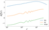 |
Fig. 1 Projected response coefficients for the WL and GCph probes and their cross-correlation for the central redshift bin (0.8 ≲ z ≲ 0.9). The shape and amplitude of the functions for different redshift pairs are analogous. For WL, the baryon acoustic oscillation wiggles are smoothed out by the projection, because the kernels are larger than the GCph ones. The different amplitude of the response is one of the main factors governing the severity of SSC. |
3 Forecasts specifics
In order to forecast the uncertainties in the measurement of the cosmological parameters, we follow the prescriptions of the Euclid forecast validation study (EC20), with some updates to the most recent results from the EC, which are used for the third Science Performance Verification (SPV) of Euclid before launch. In particular, the update concerns the fiducial value of the linear bias, the redshift distribution n(z) and the multipole binning.
Once again, the observable under study is the angular PS of probe A in redshift bin i and probe B in redshift bin j, given in the Limber approximation by Eq. (1). The PAB(kℓ, z) multi-probe power spectra are given in Eq. (13); in the following, we refer interchangeably to the probes (WL, XC, GCph) and their auto-and cross-spectra (respectively, LL, GL, GG).
3.1 Redshift distribution
First, we assume that the same galaxy population is used to probe both the WE and the GCph PS. We therefore set
 (16)
(16)
where  are respectively the distribution of sources and lenses in the i-th redshift bin. Then, the same equality applies for the total source and lens number density,
  .
.
A more realistic galaxy redshift distribution than the analytical one presented in EC20 can be obtained from simulations. We use the results from Euclid Collaboration (2021), in which the n(z) is constructed from photometric redshift estimates in a 400 deg2 patch of the Flagship 1 simulation (Potter et al. 2017), using the training-based directional neighbourhood fitting (DNF) algorithm (De Vicente et al. 2016).
The training set is a random subsample of objects with true (spectroscopic) redshifts known from the Flagship simulation. We choose the fiducial case presented in Euclid Collaboration (2021), which takes into account a drop in completeness of the spectroscopic training sample with increasing magnitude. A cut in magnitude IE < 24.5, isotropic and equal for all photometric bands, is applied, corresponding to the optimistic Euclid setting. The DNF algorithm then produces a first estimate of the photo-z, zmean, using as a metric the objects’ closeness in colour and magnitude space to the training samples. A second estimate of the redshift, zmc, is computed from a Monte Carlo draw from the nearest neighbour in the DNF metric. The final distributions for the different redshift bins, ni(z), are obtained by assigning the sources to the respective bins using their Zmean, and then taking the histogram of the zmc values in each of the bins – following what has been done in real surveys such as the Dark Energy Survey (Crocce et al. 2019; Hoyle et al. 2018).
As a reference setting, we choose to bin the galaxy distribution into 𝒩b = 10 equipopulated redshift bins, with edges
 (17)
(17)
The total galaxy number density is  . As a comparison, this was set to 30 arcmin−2 in EC20. We note that this choice of redshift binning will be discussed and varied in Sect. 5.3.
3.2 Weight functions
We model the radial kernels, or weight functions, for WL and GCph following once again EC20. Adopting the eNLA (extended non-linear alignment) prescription for modelling the intrinsic alignment (IA) contribution, the weight function  for the lensing part is given by (see e.g. Kitching et al. 2017; Kilbinger et al. 2017; Taylor et al. 2018b)
 (18)
(18)
where we define5
![Mathematical equation: ${\cal W}_i^\gamma () = {3 \over 2}{\left( {{{{H_0}} \over c}} \right)^2}{\Omega _{{\rm{m}},0}}(1 + )r()\mathop \smallint \limits_^{{_{\max }}} {{{n_i}\left( {'} \right)} \over {\bar n}}\left[ {1 - {{r()} \over {r\left( {'} \right)}}} \right]{\rm{d}}',$](/articles/aa/full_html/2024/11/aa48389-23/aa48389-23-eq46.png) (19)
(19)
and
 (20)
(20)
Finally, in Eq. (18), 𝒜IA is the overall IA amplitude, CIA a constant, ℱIA(z) a function modulating the dependence on redshift, and D(z) is the linear growth factor. More details on the IA modelling are given in Sect. 3.5.
The GCph weight function is equal to the IA one, as long as Eq. (16) holds:
 (21)
(21)
Figure 2 shows the redshift dependence of Eqs. (18) and (21), for all redshift bins. We note that we choose to include the galaxy bias term bi(z) in the PS (see Eq. (13)) rather than in the galaxy kernel, as opposed to what has been done in EC20. This is done to compute the galaxy response as described in Sect. 2.2. However, as the galaxy bias is assumed constant in each bin, the question is of no practical relevance when computing the Sijkl matrix, since the constant bias cancels out.
We note that the above definitions of the lensing and galaxy kernels  differ from the ones used in LG19. This is simply because of a different definition of the
  Limber integral, which is performed in dV in LG19 and in dz in EC20. The mapping between the two conventions is simply given by the expression for the volume element:
 (22)
(22)
and
 (23)
(23)
with A = L, G. In Fig. 2 we plot the values of  to facilitate the comparison with EC20. As outlined in Appendix A, when computing the Sijkl matrix through PySSC, the user can either pass the kernels in the form used in LG19 or the one used in EC20 – specifying a non-default convention parameter.
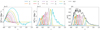 |
Fig. 2 Kernels and galaxy distribution considered in this work. The first two plots show the kernels, or weight for the two photometric probes. The analytic expressions for these are, respectively, Eqs. (18) (left, WL) and (21) (right, GCph). At high redshifts, the IA term dominates over the shear term in the lensing kernels, making them negative. The rightmost plot shows the redshift distribution per redshift bin for the sources (and lenses), as well as their sum, obtained from the Flagship 1 simulation as described in Sect. 3.1. |
3.3 Gaussian covariance
The Gaussian part of the covariance is given by the following expression:
![Mathematical equation: $Co{v_{\rm{G}}}\left[ {\hat C_{ij}^{AB}(\ell ),\hat C_{kl}^{CD}\left( {\ell '} \right)} \right] = {\left[ {(2\ell + 1){f_{{\rm{sky}}}}\Delta \ell } \right]^{ - 1}}\delta _{\ell \ell '}^{\rm{K}}$](/articles/aa/full_html/2024/11/aa48389-23/aa48389-23-eq54.png)
![Mathematical equation: $\matrix{ { \times \{ \left[ {C_{ik}^{AC}(\ell ) + N_{ik}^{AC}(\ell )} \right]\left[ {C_{jl}^{BD}\left( {\ell '} \right) + N_{jl}^{BD}\left( {\ell '} \right)} \right]} \cr { + \left[ {C_{il}^{AD}(\ell ) + N_{il}^{AD}(\ell )} \right]\left[ {C_{jk}^{BC}\left( {\ell '} \right) + N_{jk}^{BC}\left( {\ell '} \right)} \right]\} ,} \cr } $](/articles/aa/full_html/2024/11/aa48389-23/aa48389-23-eq55.png) (24)
(24)
where we use a hat to distinguish the estimators from the true spectra. The noise PS  are, for the different probe combinations,
 (25)
(25)
In the above equations,  is the Kronecker delta and
  the variance of the total intrinsic ellipticity dispersion of WL sources, where
  , with
  being the ellipticity dispersion per component of the galaxy ellipse. Some care is needed when defining the shear noise spectrum: the above equation can then also be written as
 ![Mathematical equation: $N_{ij}^{{\rm{LL}}}(\ell ) = \left[ {{{\left( {\sigma _^{(i)}} \right)}^2}/\bar n_i^{\rm{L}}} \right]\delta _{ij}^{\rm{K}}$](/articles/aa/full_html/2024/11/aa48389-23/aa48389-23-eq62.png) , that is, using the ellipticity dispersion per component instead of the total one, which is the appropriate choice for harmonic-space analyses (Hu & Jain 2004; Joachimi & Bridle 2010). We note that the average densities used in Eq. (25) are not the total number densities, but rather those in the ¿-th redshift bin. In the case of 𝒩b, equipop-ulated redshift bins, they can be simply written as
, that is, using the ellipticity dispersion per component instead of the total one, which is the appropriate choice for harmonic-space analyses (Hu & Jain 2004; Joachimi & Bridle 2010). We note that the average densities used in Eq. (25) are not the total number densities, but rather those in the ¿-th redshift bin. In the case of 𝒩b, equipop-ulated redshift bins, they can be simply written as  for both A = (L, G). Finally, we recall that ƒsky is the fraction of the total sky area covered by the survey, while ∆ℓ is the width of the multipole bin centred on a given ℓ. From Sect. 3.1 we have that
  , while we set σє = 0.37 (from the value
  reported in Euclid Collaboration 2019) and ƒsky = 0.356 (corresponding to ΩS = 14 700 deg2). We have now all the relevant formulae for the estimate of the Gaussian and the SSC terms of the covariance matrix. To ease the computation of Eq. (24) we have prepared an optimised Python module, Spaceborne_covg6, available as a public repository.
In the context of the present work, we do not consider the other non-Gaussian contribution to the total covariance matrix, the so-called connected non-Gaussian (cNG) term. This additional non-Gaussian term has been shown to be subdominant with respect to the Gaussian and SSC terms for WL both in Barreira et al. (2018a) and in Upham et al. (2022). For what concerns galaxy clustering, Wadekar et al. (2020) showed that the cNG term was subdominant, but this was for a spectroscopic sample so (i) they had a much larger contribution from shot-noise-related terms compared to what is considered here for the Euclid photometric sample, and (ii) they considered larger and more linear scales than in the present study. Lacasa (2020) showed that the cNG term in the covariance matrix of GCph only impacts the spectral index ns and HOD parameters, but there are a few differences between that analysis and the present work, such as the modelling of galaxy bias. Thus it is still unclear whether the cNG term has a strong impact on cosmological constraints obtained with GCph. Quantifying the impact of this term for the 3×2pt analysis with Euclid settings is left for future work.
3.4 Cosmological model and matter power spectrum
We adopt a flat w0waCDM model, that is, we model the dark energy equation of state with a Chevallier-Polarski-Linder (CPL) parametrisation (Chevallier & Polarski 2001; Linder 2005):
 (26)
(26)
We also include a contribution from massive neutrinos with total mass equal to the minimum allowed by oscillation experiments (Esteban et al. 2020) ∑mv = 0.06 eV, which we do not vary in the FM analysis. The vector of cosmological parameters is then
 (27)
(27)
with Ωm,0 and Ωb,0 being respectively the reduced density of total and baryonic matter today, h is the dimensionless Hubble parameter defined as H0 = 100 h km s−1 Mpc−1 where H0 is the value of the Hubble parameter today, ns the spectral index of the primordial power spectrum and σ8 the root mean square of the linear matter density field smoothed with a sphere of radius 8 h−1 Mpc. We follow EC20 for their fiducial values that are
 (28)
(28)
This parameter vector then is used as input for the evaluation of the fiducial linear and non-linear matter PS; for the purpose of validating our forecasts against the EC20 results, we use the TakaBird recipe, that is, the HaloFit version updated in Takahashi et al. (2012) with the Bird et al. (2012) correction for massive neutrinos. For the results shown in this paper, however, we update the non-linear model to the more recent HMCode2020 recipe, (Mead et al. 2021), which includes a baryonic correction parameterised by the log10(TAGN/K) parameter, characterising the feedback from active galactic nuclei (AGN). This is implemented in CAMB7 (Lewis et al. 2000) and, at the time of writing, is planned to be included in CLASS8 (Blas et al. 2011) as well. Because of this, we add a further free parameter in the analysis, log10(TAGN/K), with a fiducial value of 7.75.
3.5 Intrinsic alignment model
We use the eNLA model as in EC20, setting 𝒞IA = 0.0134 and
![Mathematical equation: ${{\cal F}_{{\rm{IA}}}}() = {(1 + )^{{\eta _{{\rm{IA}}}}}}{\left[ {\langle L\rangle ()/{L_ \star }()} \right]^{{\beta _{{\rm{IA}}}}}},$](/articles/aa/full_html/2024/11/aa48389-23/aa48389-23-eq69.png) (29)
(29)
where 〈L〉(z)/L⋆(z) is the redshift-dependent ratio of the mean luminosity over the characteristic luminosity of WL sources as estimated from an average luminosity function (see e.g. Joachimi et al. 2015, and references therein). The IA nuisance parameters vector is
 (30)
(30)
with fiducial values – following EC20
 (31)
(31)
All of the IA parameters except for 𝒞IA are varied in the analysis.
3.6 Linear galaxy bias and multiplicative shear bias
Following EC20 we model the galaxy bias as scale-independent. As for the redshift dependence, we move beyond the simple analytical prescription of EC20 and use the fitting function presented in Euclid Collaboration (2021), obtained from direct measurements from the Euclid Flagship galaxy catalogue, based in turn on the Flagship 1 simulation:
 (32)
(32)
setting (A, B, C) = (0.81,2.80,1.02).
The galaxy bias is modelled to be constant in each bin with the fiducial value obtained by evaluating Eq. (32) at effective values  computed as the median of the redshift distribution considering only the part of the distribution at least larger than 10% of its maximum. We choose to use the median instead of the mean since, for equipopulated bins – as can be seen from the rightmost panel of Fig. 2 – the galaxy distribution of the last bins is highly skewed, and the value of the bias computed at the mean is potentially less accurate; this choice does not, on the other hand, affect the galaxy bias values in the first bins sensibly.
The  values obtained in this way are
 (33)
(33)
We therefore have 𝒩b additional nuisance parameters:
 (34)
(34)
with fiducial values
 (35)
(35)
The modelling of galaxy bias just described is the same used in EC20, with different fiducial values.
We can take a further step forward towards the real data analysis by including the multiplicative shear bias parameters, m, defined as the multiplicative coefficient of the linear bias expansion of the shear field γ (see e.g. Cragg et al. 2023):
 (36)
(36)
with  the measured shear field, γ the true one, m the multiplicative and c the additive shear bias parameters (we do not consider the latter in the present analysis, as we assume it will be corrected in the shear data processing pipeline). The multiplicative shear bias can come from astrophysical or instrumental systemat-ics (such as the effect of the point spread function – PSF), which affect the measurement of galaxy shapes. We take the mi parameters (one for each redshift bin) as constant and with a fiducial value of 0 in all bins. To include this further nuisance parameter, one just has to update the different angular PS as
 (37)
(37)
where mi is the i-th bin multiplicative bias, and the GCph spectrum is unchanged since it does not include any shear term. We then have
 (38)
(38)
with fiducial values
 (39)
(39)
Finally, we introduce the ∆zi parameters to allow for uncertainties over the first moments of the photometric redshift distribution (argued to have the largest impact on the final constraints in Reischke 2024). We then have (Troxel et al. 2018; Abbott et al. 2018; Tutusaus et al. 2020):
 (40)
(40)
which adds new entries to our nuisance parameter vector:
 (41)
(41)
with fiducial values:
 (42)
(42)
These nuisance parameters – unless specified otherwise – are varied in the Fisher analysis so that the final parameters vector is

and

both composed of 𝒩p = 7 + 3 + 3𝒩b = 3𝒩b + 10 elements.
3.6.1 Higher-order bias
To compute the galaxy–galaxy and galaxy–galaxy lensing probe response terms (Eqs. (14) and (15)) we need the second-order galaxy bias b(2)(z). To do this, we follow Appendix C of LG19, in which this is estimated following the halo model9 as (Voivodic & Barreira 2021; Barreira et al. 2021)
 (43)
(43)
with
 (44)
(44)
the galaxy number density, ΦMF(M, z) the halo mass function (HMF),  (M, z) the i-th order halo bias, and 〈N|M〉 the average number of galaxies hosted by a halo of mass M at redshift z (given by the halo occupation distribution, HOD). These are integrated over the mass range log M ∈ [9,16], with the mass expressed in units of solar masses (we don't include h in our units). The expression for the i-th order galaxy bias (Eq. (43)) is the same as Eq. (C.2) of LG19, but here we are neglecting the scale dependence of the bias evaluating it at k = 0 so that u(k | M = 0, z) = 1, u(k | M, z) being the Fourier Transform of the halo profile. Strictly speaking, this gives us the large-scale bias, but it is easy to check that the dependence on k is negligible over the range of interest.
Although Eq. (43) allows the computation of both the first and second-order galaxy bias, we prefer to use the values of b(1)(z) measured from the Flagship simulation for the selected galaxy sample; this is to maintain consistency with the choices presented at the beginning Sect. 3.6. For each redshift bin, we vary (some of) the HOD parameters to fit the measured b(1)(z), thus getting a model for  . We then compute
  using as an additional ingredient the following relation between the first and second-order halo bias, which approximates the results from separate universe simulations (Lazeyras et al. 2016) within the fitting range
  :
:
![Mathematical equation: $\matrix{ {b_{(2)}^{\rm{h}}(M,) = 0.412 - 2.143b_{(1)}^{\rm{h}}(M,)} \hfill \cr {\,\,\,\,\,\, + 0.929{{\left[ {b_{(1)}^{\rm{h}}(M,)} \right]}^2} + 0.008{{\left[ {b_{(1)}^{\rm{h}}(M,)} \right]}^3}.} \hfill \cr } $](/articles/aa/full_html/2024/11/aa48389-23/aa48389-23-eq94.png) (45)
(45)
Finally, we plug the  values obtained in this way back into Eq. (43) to get the second-order galaxy bias. The details of the HMF and HOD used and of the fitting procedure are given in Appendix B.
3.7 Data vectors and Fisher matrix
Up to now, we have outlined a fully general approach, without making any assumptions about the data. We now need to set data-related quantities.
First, we assume that we will measure  in ten equally populated redshift bins over the redshift range (0.001,2.5). When integrating Eq. (1) in dz, zmax must be larger than the upper limit of the last redshift bin to account for the broadening of the bin redshift distribution due to photo-z uncertainties. We have found that the
  stop varying for zmax ≥ 4, which is what we take as the upper limit in the integrals over z. This also means that we need to extrapolate the bias beyond the upper limit of the last redshift bin; we then take its value as constant and equal to the one in the last redshift bin, that is, b(z > 2.501) = b10.
Second, we assume the same multipole limits as in EC20, and therefore examine two scenarios, as follows:
pessimistic:

optimistic:

Then, for the multipole binning, instead of dividing these ranges into Nℓ (logarithmically equispaced) bins in all cases as is done in EC20, we follow the most recent prescriptions of the EC and proceed as follows:
we fix the centres and edges of 32 bins (as opposed to 30) in the ℓ range [10,5000] following the procedure described in Appendix C. This will be the ℓ configuration of the optimistic WL case.
The bins for the cases with ℓmax < 5000, such as WL pessimistic, GCph, or XC, are obtained by cutting the bins of the optimistic WL case with ℓcentre > ℓmax. This means that instead of fixing the number of bins and having different bin centres and edges as done in EC20, we fix the bins’ centres and edges and use a different number of bins, resulting in, for example,
 .
.
The number of multipole bins is then  and
and  in the pessimistic case and
  and
and  in the optimistic case. In all these cases, the angular PS are computed at the centre of the ℓ bin, as done in EC20.
We note that, because of the width of the galaxy – and, more importantly, lensing – kernels, a given fixed ℓmax will not correspond to a unique kmax value. A more accurate approach could be, for example, to use the k-cut method presented in Taylor et al. (2018a), which leverages the BNT (Bernardeau-Nishimichi-Taruya) transform (Bernardeau et al. 2014) to make the lensing kernels separable in z, hence allowing for a cleaner separation of scales. We leave the investigation of this important open issue to dedicated work.
As mentioned, we consider the different probes in isolation, as well as combine them in the '3×2pt' analysis, which includes three 2-point angular correlation functions (in harmonic space):  and
and  . The ℓ binning for the 3×2pt case is the same as for the GCph one.
The covariance matrix and the derivatives of the data vector w.r.t. the model parameters are the only elements needed to compute the FM elements. The one-dimensional data vector C is constructed by simply compressing the redshift and multipole indices (and, in the 3×2pt case, the probe indices) into a single one, which we call p (or q). For Gaussian-distributed data with a parameter-independent covariance, the FM is given by:
 (46)
(46)
We refer the reader to EC20 for details on the convergence and stability of the Fisher matrix and derivatives computations.
We note that the size of the 3×2pt covariance matrix quickly becomes large. For a standard setting with 𝒩b = 10 redshift bins, there are respectively (55,100, 55) independent redshift bin pairs for (WL, XC, GCph), to be multiplied by the different 𝒩ℓ. In general, Cov will be a 𝒩C × 𝒩C matrix with
![Mathematical equation: $\eqalign{ & {{\cal N}_C} = \left[ {{{\cal N}_{\rm{b}}}\left( {{{\cal N}_{\rm{b}}} + 1} \right)/2} \right]\left[ {{\cal N}_\ell ^{{\rm{WL}}} + {\cal N}_\ell ^{{\rm{GCph}}}} \right] + {\cal N}_{\rm{b}}^2{\cal N}_\ell ^{{\rm{XC}}} \cr & \,\,\,\,\,\,\,\,\, = \left[ {{{\cal N}_{\rm{b}}}\left( {{{\cal N}_{\rm{b}}} + 1} \right) + {\cal N}_{\rm{b}}^2} \right]{\cal N}_\ell ^{3 \times 2{\rm{pt}}}, \cr} $](/articles/aa/full_html/2024/11/aa48389-23/aa48389-23-eq108.png) (47)
(47)
where the second line is for the 3×2pt case, which has the same number of ℓ bins for all probes, and
![Mathematical equation: ${{\cal N}_C} = \left[ {{{\cal N}_{\rm{b}}}\left( {{{\cal N}_{\rm{b}}} + 1} \right)/2} \right]{\cal N}_\ell ^{{\rm{WL}}/{\rm{GCph}}},$](/articles/aa/full_html/2024/11/aa48389-23/aa48389-23-eq109.png) (48)
(48)
for the WL and GCph cases. As an example, we have  .
.
Being diagonal in ℓ, most elements of this matrix will be null in the Gaussian case. As shown in Fig. 3, this is no longer true with the inclusion of the SSC contribution, which makes the matrix computation much more resource-intensive. The use of the Numba JIT compiler10 can dramatically reduce the CPU (for Central Processing Unit) time from about 260 s to about 2.5 s for the Gaussian + SSC 3×2pt covariance matrix (the largest under study) on a normal laptop working in single-core mode.
Given the highly non-diagonal nature of the Gaussian + SSC covariance, we might wonder whether the inversion of this matrix (which is needed to obtain the FM, see Eq. (46)) is stable. To investigate this, we compute the condition number of the covariance, which is defined as the ratio between its largest and smallest eigenvalues and in this case of order 1013. This condition number, multiplied by the standard numpy float64 resolution (2.22 × 10⁻¹⁶), gives us the minimum precision that we have on the inversion of the matrix, of about 10−3. This means that numerical noise in the matrix inversion can cause, at most, errors of order 10−3 on the inverse matrix. Hence, we consider the inversion to be stable for the purpose of this work.
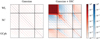 |
Fig. 3 Correlation matrix in log scale for all the statistics of the 3×2pt data-vector in the G and GS cases. The positive and negative elements are shown in red and blue, respectively. The Gaussian covariance is block diagonal (i.e. it is diagonal in the multipole indices, but not in the redshift ones; the different diagonals appearing in the plot correspond to the different redshift pair indices, for ℓ1 = ℓ2). The overlap in the WL kernels makes the WL block in the Gaussian + SSC covariance matrix much more dense than the GCph one. |
4 Forecast code validation
In order to validate the SSC computation with PySSC, we compare the 1σ forecast uncertainties (which correspond to a 68.3% probability, due to the assumptions of the FM analysis) obtained using two different codes independently developed by two groups, which we call A and B. To produce the FM and the elements needed for its computation (the observables, their derivatives and the covariance matrix), group A uses a private11 code fully written in Python and group B uses CosmoSIS12 (Jennings et al. 2016). As stated in the introduction, the only shared feature of the two pipelines is the use of PySSC (to compute the Sijkl matrix). For this reason, and because the SSC is not considered in isolation but added to the Gaussian covariance, we compare the forecast results of the two groups both for the Gaussian and Gaussian + SSC cases.
Following EC20, we consider the results to be in agreement if the discrepancy of each group’s results with respect to the median – which in our case equals the mean – is smaller than 10%. This simply means that the A and B pipelines’ outputs are considered validated against each other if
 (49)
(49)
with  the 1σ uncertainty on the parameter α for group A. The above discrepancies are equal and opposite in sign for A and B.
The marginalised uncertainties are extracted from the FM Fαβ, which is the inverse of the covariance matrix Cαβ of the parameters: (F−1)αβ = Cαβ. The unmarginalised, or conditional, uncertainties are instead given by  . We then have
 (50)
(50)
The uncertainties found in the FM formalism constitute lower bounds, or optimistic estimates, on the actual parameters’ uncertainties, as stated by the Cramér-Rao inequality.
In the following, we normalise σα by the fiducial value of the parameter θα, in order to work with relative uncertainties:  , again with i = A,B. If a given parameter has a fiducial value of 0, such as wa, we simply take the absolute uncertainty. The different cases under examination are dubbed 'G', or 'Gaussian', and 'GS', or 'Gaussian + SSC’. The computation of the parameters constraints differs between these two cases only by the covariance matrix used in Eq. (46) to compute the FM:
 (51)
(51)
As mentioned above, we repeat the analysis for both Euclid’s photometric probes taken individually, WL and GCph, as well as for the combination of WL, GCph, and their cross-correlation XC, the 3×2pt.
For the reader wanting to validate their own code, we describe the validation process in Appendix A. Here we sketch the results of the code validation: in Fig. 4, we show the percent discrepancy as defined in Eq. (49) for the 3×2pt case. Similar results have been obtained for the GCph and WL cases, both for the optimistic and pessimistic settings specified in Sect. 3.7. The constraints are all found to satisfy the required agreement level (less than 10% discrepancy with respect to the mean). In light of these results, we consider the two forecasting pipelines validated against each other. All the results presented in this paper are the ones produced by group A.
 |
Fig. 4 Percentage discrepancy of the normalised 1σ uncertainties with respect to the mean for the WL probe, both in the G and GS cases (optimistic settings). The index i = A, B indicates the two pipelines, whilst α indexes the cosmological parameter. The desired agreement level is reached in all cases (WL, GCph probes and pessimistic case not shown). |
5 SSC impact on forecasts
We investigate here how the inclusion of SSC degrades the constraints with respect to the Gaussian case. To this end, we look in the following at the quantity
 (52)
(52)
where σG(θ) and σGS(θ) are the usual marginalised uncertainties on the parameter θ computed, as detailed above, with Gaussian or Gaussian + SSC covariance matrix. We run θ over the set of cosmological parameters listed in Eq. (27), that is, θ ∈ {Ωm,0, Ωb,0, w0, wa, h, ns, σ8}.
In addition, we examine the FoM as defined in Albrecht et al. (2006), a useful way to quantify the joint uncertainty on several parameters. In this work, we parameterise the FoM following EC2O: for two given parameters θ1 and θ2, we have
 (53)
(53)
This quantity is inversely proportional to the area of the 2σ confidence ellipse in the plane spanned by the parameters (θ1, θ2).  is the Fisher submatrix obtained by marginalising over all the parameters but θ1 and θ2, and is computed by inverting Fαβ (that is, taking the parameters’ covariance matrix), removing all the rows and columns but the ones corresponding to θ1 and θ2 and reinverting the resulting 2 × 2 matrix. In the following, we mainly focus on the joint uncertainty on the dark energy equation of state parameters w0 and wa, and unless specified otherwise we use the notation FoM = FoMw0wa. However, the FoM can help quantify the joint uncertainty on different sets of parameters, such as (Ωm,0 − S8), with S8 = σ8(Ωm,0/0.3)0. 5 (see e.g. Abbott et al. 2022).
We also use the notation ℛ(FoM) as a shorthand for FoMGS/FoMG. We note that, since we expect the uncertainties to be larger for the GS case, we have ℛ(θ) > 1, and the FoM being inversely proportional to the area of the uncertainty ellipse, ℛ(FoM) < 1.
Ratio between the GS and G conditional uncertainties for all cosmological parameters and probes in the reference case, for the optimistic settings.
5.1 Reference scenario
Let us start by considering the case with 𝒩b = 10 equipopulated redshift bins. To isolate the impact of SSC and gain better physical insight, we begin by computing the conditional uncertainties as described in the last section.
Table 1 gives the values of the ℛ ratios for the different parameters in the optimistic scenarios, for the single probes and their combination.
In accordance with previous results in the literature, we find that the WL constraints are dramatically impacted by the inclusion of SSC: as found in Barreira et al. (2018a) (cf. their Fig. 2), all cosmological parameters are affected, with wa and h being impacted the least and (Ωm,0, σ8, log10(TAGN/K)) the most. This is because the SSC effect is essentially an unknown shift, or perturbation, in the background density within the survey volume, and is hence degenerate with the parameters which more closely relate to the amplitude of the signal. Being this a nonlinear effect, its impact is also tied to the amount of power on small scales, which in turn is influenced by the baryonic boost, parameterised by log10(TAGN/K) in our model.
The results in Table 1 also show that GCph is not as strongly affected by SSC – with the exception of the log10(TAGN/K) constraint. This is an expected result (see e.g. Bayer et al. 2023), mainly driven by the fact that the GCph probe response coefficients are lower (in absolute value) than the WL ones, as can be seen in Fig. 1. This is due to the additional terms that account for the response of the galaxy number density ng (see Eq. (14)), which is itself affected by the super-survey modes. Additionally, as can be seen from Fig. 2, all WL kernels have non-zero values for z → 0, contrary to the GCph ones. In this limit, the effective volume probed by the survey tends to 0, hence making the variance of the background modes σ2 tend to infinity. We thus have a larger Sijkl matrix, which is one of the main factors driving the amplitude of the SSC. We also note that the importance of bary-onic feedback for GCph depends on the galaxy bias model used; it will likely be reduced when using a non-linear bias expansion, needed for an accurate analysis on small scales (Desjacques et al. 2018). Both topics are still active areas of research, and we leave the characterisation of the SSC impact with the inclusion of higher-order bias terms for future work.
The impact for the full 3×2pt case sits in principle in between the two extremes as a consequence of the data vector containing the strongly affected WL probe, and the less affected GCph one. However, this is clearly apparent only in the case of Ωm,0, since it is the only cosmological parameter for which the WL constraining power is higher than the GCph one; for the other parameters, the trend resembles very closely the one found for GCph, because of its dominant contribution to the 3×2pt precision.
Lastly, the contribution from the XC probe is again an intermediate case, as can be anticipated by looking at its response coefficient in Fig. 1, so the final impact on the FM elements will be intermediate between the WL and GCph cases, as the ℛ(θ) values in Table 1 indeed show.
Having explored the impact of SSC on the conditional uncertainties, we move on to analyse a more realistic scenario, namely letting the parameters in the analysis free to vary, as opposed to fixing them to their fiducial values.
To compute the 1σ uncertainties in this case, we marginalise over all cosmological and nuisance parameters. We add Gaussian priors of standard deviation σp = 5 × 10⁻⁴ on the multiplicative shear bias parameters, and of σp = σz(1 + z) with σz = 0.002 (see Euclid Collaboration 2024 and references therein) on the dzi parameters. We also include a Gaussian prior of σp = 0.06 on log10(TAGN/K), which roughly matches the prior range recommended in Mead et al. (2021). To add these priors in the FM analysis, it is sufficient to add  to the appropriate diagonal elements of the G and GS FMs (
 being the value of the prior on parameter α).
The results of this analysis, which we take as our reference scenario, are shown in Table 2 and in Figs. 5–8. For the WL case, marginalisation over all cosmological and nuisance parameters leads to the result that the SSC has now a very minor impact – of a maximum of about 13% in the optimistic case -on the constraints and the FoM: again, this is in line with what found in Barreira et al. (2018a). We also compute the Ωm,0 − S8 FoM, after projecting the FM to the new parameter space with S8 replacing σ8 (see e.g. Coe 2009). This drops from 336 to 292 in the optimistic case, corresponding to a ratio of 0.87 (0.92 in the pessimistic case), closely mirroring the results found for FoMw0wa.
These values are actually easily explained: marginalising over cosmological and nuisance parameters, particularly if these are degenerate with the amplitude of the signal, dilutes the SSC effect in a larger error budget; because of this, it is the relative rather than the absolute impact of SSC that decreases. Indeed, marginalising over additional parameters is formally equivalent to having additional covariance. The parameters that mostly change the SSC impact when marginalised over are the cosmo-logical ones, but the multiplicative nuisance parameters mi and bi also play a role: adding these to the set of free parameters introduces a degeneracy between these and the overall amplitude of  . Such a degeneracy is a mathematical one present on the whole ℓ range. As a consequence, the constraints on all the parameters and the FoM are degraded in a way that is independent of the presence of SSC. This is shown in Figs. 5 and 6, which respectively exhibit the relative uncertainty
  and the FoMs in the G and GS cases for each parameter, if we marginalise or not over nuisance parameters. Letting these free to vary, i.e. marginalising over them, tends to increase the uncertainty on cosmological parameters way more than including SSC, and this is even more true when these nuisance parameters are simply multiplicative such as bi and mi.
This of course does not mean that varying more parameters improves the constraints. Indeed, the uncertainties on all parameters increase (hence the FoM decreases) with respect to the case of conditional uncertainties introduced above.
The same reasoning applies to the GCph probe, for which the SSC impact drops now to a subpercent level in the pessimistic case and to about 10% at most in the optimistic case (on w0 and the two FoMs). As mentioned above, for GCph, one of the reasons behind the observed decrease in the (already low) SSC relative impact is the marginalisation over the galaxy bias parameters, which are perfectly degenerate with the amplitude of the signal and over which we impose no prior.
On the other hand, the results for the 3×2pt case show that the SSC still matters. The additional information carried by the GCph and XC data allows the partial breaking of parameter degeneracies, including those with probe-specific systematics such as mi and bi, hence making the scale-dependent increase of the uncertainties due to the inclusion of SSC important again. For this reason, in this case, the 3×2pt does not follow the behaviour of the single probes as seen earlier. In particular, the dark energy FoM, whose increase with respect to present surveys is one of the main objectives of the Euclid mission, is highly degraded – by a factor of about 2 in the optimistic case. This is mainly due to the large impact on the dark energy equation of state parameters, showing the importance of accounting for SSC in upcoming LSS analyses. The same conclusion holds for  , with a slightly larger ℛ value driven by the lower impact on σ8 w.r.t. w0 and wa. In Fig. 7 we show the comparison of the 2D contours for all cosmological parameters between G and GS in the case of the 3×2pt analysis, in the optimistic case; the most impacted parameters in this case are Ωm,0, w0 and wa. In addition, this shows that SSC does not seem to strongly affect the correlations between cosmological parameters.
Table 2 also shows the ratios in the 'GCph diag.' case, in which we neglect the GCph cross-reshift elements (i.e. we take the diagonal of the  matrix for each ℓ value). This choice is sometimes made because of the large sensitivity of such measurements on the photometric redshift calibration, which is less of an issue for WL due to its broad kernel. The values show the robustness of our conclusions even in this case, with the ℛ values being very close to the standard case both for GCph and for the 3×2pt.
We note that these conclusions depend on the scale cuts imposed in the data vector, as can be seen from the lower FoM decrease (and of the SSC impact as a whole, with some exceptions) in the pessimistic case, in line with what found in Lacasa (2020) for GCph. This is a direct consequence of the larger amount of non-linear modes included in the data vectors, which as mentioned previously are more subject to mode coupling and hence contribute more to SSC. For WL, it should be noted that the diagonal elements of the total covariance matrix are always dominated by the Gaussian contribution, because of the presence of the scale-independent shape noise (see Eq. (24) for A = B = L), which largely dominates over the SSC on small scales. This is consistent with the results of Upham et al. (2022) showing that the diagonal elements of the WL total covariance matrix are more and more dominated by the Gaussian term as we move to higher ℓ. This is also the case for GCph, although the predominance of the Gaussian term along the diagonal is less pronounced because of the smaller contribution of shot noise.
As mentioned above, more sophisticated choices of scale cuts, e.g. through the use of the BNT transform, will allow decreasing the high-k contribution to a given ℓ mode, hence mitigating the SSC impact more than the "hard" angular scale cut considered here (and in EC20). We leave the investigation of this point to a forthcoming publication.
To conclude this section, it is also worth looking at the impact of SSC on the astrophysical nuisance parameters. Indeed, although an issue to be marginalised over when looking at cos-mological ones, the IA and the galaxy bias parameters are of astrophysical interest. We show the impact of SSC on the constraints on these quantities in Fig. 8, as well as on the galaxy bias and the multiplicative shear bias parameters.
For IA-related nuisance parameters, the uncertainty increase due to SSC is lower than 5% when considering WL-only, and below 1% for the full case. The multiplicative shear bias parameters are affected by a similar amount (up to around 10% for the last bin) and in a similar way for WL and the 3×2pt. As for the galaxy bias parameters, the impact is modest for GCph but quite significant (between 30 and 40%) for the 3×2pt. These results are analogous to what was found before for the cosmological parameters: in the marginalised 3×2pt case the impact of SSC is more apparent, since many degeneracies are broken thanks to the probes combination and cross-correlation.
In this case, contrary to the IA parameters, the uncertainty on bi and mi in each of the ten redshift bins is significantly affected by SSC. This is because both of these nuisance parameters simply act as a multiplicative factor on the power spectrum and are thus highly degenerated with the effect of SSC. Again, this is related to the fact that the first-order effect of SSC is to modulate the overall clustering amplitude because of a shift in the background density δb. For the mi parameters, we remind that a tight (while realistic) prior is imposed, keeping the SSC uncertainty increase, and hence the ℛ ratio, quite low even for the full 3 × 2pt. We note that going beyond the linear approximation for the modelling of the galaxy bias will add more nuisance parameters, thus degrading the overall constraints on cosmological parameters and further reducing the relative impact of SSC.
Ratio between the GS and G marginalised uncertainties for all cosmological parameters and the FoM in the reference scenario, for the optimistic and pessimistic settings.
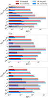 |
Fig. 5 Marginalised and conditional optimistic 1σ uncertainties on the cosmological parameters, relative to their corresponding fiducial values (in percent units), in both the G and GS cases for WL, GCph, and the 3×2pt. We highlight the logarithmic scale on the x-axis, made necessary by the large range of values. The values in these plots have been used to compute the ratios in Tables 1 and 2. |
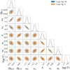 |
Fig. 7 Contour plot for the G and GS constraints, considering the full 3×2pt analysis in the optimistic case, in the reference scenario. The two shaded regions of the ellipses represent the 1 and 2σ contours. For clarity, the nuisance parameters are shown separately in Fig. 8 and the log10(TAGN/K) parameter name has been shortened to log(T). |
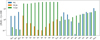 |
Fig. 8 Percent increase of the marginalised 1σ uncertainty of the nuisance parameters, for all probe choices, in the optimistic case and for the reference scenario. |
5.2 Non-flat cosmologies
In the previous section, we investigate the SSC on the cosmological parameters under the assumption of a flat model. Actually, the requirement on the FoM assessed in the Euclid Red Book (Laureijs et al. 2011) refers to the case with the curvature as an additional free parameter to be constrained, that is, the non-flat w0waCDM model. This is why in EC20 are also reported the marginalised uncertainties for the parameter ΩDE,0, with a fiducial value  to be consistent with a flat universe. It is then worth wondering what the impact of SSC is in this case too. This is summarised in Table 3, where we now also include the impact on ΩDE,0.
A comparison with the results in Table 2 is quite hard if we look at the single parameters. Indeed, opening up the parameter space by removing the flatness assumption introduces additional degeneracy among the parameters controlling the background expansion, which are thus less constrained whether SSC is included or not. We can nevertheless note again that, for the marginalised uncertainties, 3×2pt is still the most impacted probe; the difference between pessimistic and optimistic scenarios is now less evident with ℛ(θ) increasing or decreasing depending on the parameter and probe considered.
Once more, the most affected parameters for WL are (Ωm,0, σ8), the uncertainties on which are now further degraded by the fact that they correlate with the parameter ΩDE,0 which is also affected. Although (w0, wa) are also degraded by the SSC, a sort of compensation is at work, so that the overall decrease in the FoM is similar to the case with the flatness prior. The motivations that make GCph much less affected still hold when dropping the flatness prior, explaining the corresponding ℛ(θ) values.
We also note a slight increase of ℛ(FoM) in the 3×2pt optimistic case, meaning a smaller degradation of the FoM due to SSC. The dark energy FoM indeed degrades by 52% (45%) in the non-flat case vs. 50% (58%) for the flat case in the pessimistic (optimistic) scenario, while  degrades by 47% (35%) in the non-flat case vs. 43% (41%) for the flat case in the pessimistic (optimistic) scenario. This can be qualitatively explained by noting that the decrease of both FoM(G) and FoM(GS) is related to a geometrical degeneracy which is the same on all scales, whether or not they are affected by the increase in uncertainty due to the SSC inclusion.
Overall, these results suggest a dependence of the SSC significance on both the number and type of parameters to be constrained. Qualitatively, we can argue that SSC is more or less important depending on whether the additional parameters (with respect to the reference case of a flat model) introduce degeneracies which are or not scale-dependent and how strong is the degeneracy between these parameters and the amplitude of the power spectrum. To give an example, in future works lens magnification effects should be included in the analysis as these were shown to have a significant impact on cosmological constraints (Unruh et al. 2020). From our results, we can anticipate that the inclusion of magnification-related nuisance parameters will further dilute the impact of SSC.
 |
Fig. 9 Ratio between WL and 3×2pt marginalised uncertainties computed by including or neglecting the SSC contribution, as a function of the number of (equally populated) redshift bins, for the pessimistic and optimistic cases. |
5.3 Dependence on redshift binning
The results summarised in Tables 1–3 were obtained for a fixed choice of number and type of redshift bins. We investigate here how the results depend on these settings given that we expect both the G and GS constraints to change as we vary the number and type of bins. We consider again the reference scenario introduced in Sect. 5.1, that is, the case of flat models, marginalising over the full set of nuisance parameters while imposing Gaussian priors over some of them. In this section we only consider the WL and 3×2pt cases, since as we have seen SSC has a modest impact on GCph.
Let us first consider changing the number of redshift bins 𝒩b. We show the scaling of ℛ(θ) as a function of 𝒩b for the WL and 3×2pt probes, respectively, in Fig. 9 – for both the pessimistic and optimistic assumptions. The most remarkable result is the weak dependence of ℛ(x) w.r.t. 𝒩b, as can be inferred from the small y range spanned by the curves – see e.g. the bottom right panel, for the FoM. More specifically, the scaling of ℛ(θ) with 𝒩b depends on the parameter and the probe one is looking at. It is quite hard to explain the observed trends because of the interplay of different contrasting effects. For instance, a larger number of bins implies a smaller number density in each bin, and hence a larger shot noise. As a consequence, the SSC contribution to the total covariance for the diagonal elements will likely be more and more dominated by the Gaussian component because of the larger shot and shape noise terms. However, this effect also depends on the scale so that, should the SSC be the dominant component on the scales to which a parameter is most sensitive, the impact should still be important. On the other hand, a larger number of bins also comes with a larger number of nuisance parameters which, as shown above, leads to a reduction of the SSC impact. Quantifying which actor plays the major role is hard which explains the variety of trends in the different panels.
As a further modification to the reference settings, we can change how the redshift bins are defined. We have up to now considered equipopulated (EP) bins so that the central bins cover a smaller range in z, because of the larger source number density. As an alternative, we divide the full redshift range into 𝒩b bins with equal redshift support (‘equidistant’, ED), and recompute the FM forecasts with and without SSC. We show the FoM ratio as a function of the number of bins for EP and ED bins considering WL (left) and 3×2pt (right) probes in the optimistic scenario in Fig. 10. We note that finding the exact number and type of redshift bins used to maximise the constraining power of Euclid is outside the scope of this paper; this effort is indeed brought forward in the context of the SPV exercise.
In order to qualitatively explain these results, let us first consider the WL case. Given that the bins are no longer equipopulated, the number density of galaxies will typically be larger in the lower redshift bins than in the higher ones. As a consequence, the larger the number of bins, the higher the shape noise in the higher redshift bins so that the SSC will be subdominant in a larger number of bins, which explains why its impact decreases (i.e. ℛ(FoM) increases) with 𝒩b. Nevertheless, the impact of SSC will be larger than in the EP case since SSC will dominate in the low redshift bins which are the ones with the largest signal-to-noise ratio. This effect is small, and the difference in ℛ(FoM) between ED and EP is no larger than 3–5%.
When adding GCph and XC into the game, the impact of SSC is determined by a combination of contrasting effects. On the one hand, we can repeat the same qualitative argument made for WL also for GCph and XC13 thus pointing at ℛ(FoM) increasing with 𝒩b. The larger the number of bins, the narrower they are, and the smaller the cross-correlation between them hence the smaller the Gaussian covariance. This in turn increases the number of elements in the data vector whose uncertainty is dominated by the SSC. Should this effect dominate, we would observe a decrease of ℛ(FoM) with 𝒩b with the opposite trend if it is the variation of the shape and shot noise to matter the most. This qualitative argument allows us then to roughly explain the non-monotonic behaviour of ℛ(FoM) we see in the right panel of Fig. 10.
It is worth remarking, however, that the overall change of ℛ(FoM) for subsequent ED (or EP) bins over the range in 𝒩b is smaller than ~5% which is also the maximum value of the difference between ℛ(FoM) values for EP and ED bins once 𝒩b is fixed.
The analysis in this section motivates us to argue that the constraints and FoM degradation due to SSC have a weak dependence on the redshift binning scheme.
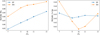 |
Fig. 10 FoM ratio vs the number of EP and ED гedshift bins for WL (left) and 3×2pt (right) in the optimistic scenario. The blue curves in this plot match the ones in the bottom right panel of Fig 9 in the optimistic case, for the corresponding probes. |
5.4 Requirements on prior information
The results in the previous paragraph show that the SSC may dramatically impact the constraints on the cosmological parameters. As a consequence, the 3×2pt FoM is reduced by up to ~ 50% with respect to the case when only the Gaussian term is included in the total covariance. This decrease in the FoM should actually not be interpreted as a loss of information due to the addition of the SSC. On the contrary, one can qualitatively say that removing SSC from the error budget is the same as adding information that is not actually there. It is nevertheless interesting to ask which additional information must be added to recover the Gaussian FoM, which is usually taken as a reference for gauging the potential of a survey. This information can come from priors on the nuisance (or cosmological) parameters. In the following section, we investigate the former option by adding Gaussian priors on the galaxy and multiplicative shear bias parameters.
To this end, we consider the realistic case of a flat model plus the galaxy bias and multiplicative shear bias as nuisance parameters. As a simplifying assumption, we assume that all the 𝒩b bias values bi are known with the same percentage uncertainty εb = σb,i/bfid, i, while we put the same prior σm on all the mi parameters (having set the fiducial value mfid to 0). We then compute the FoM with and without SSC for the 3×2pt probe in the optimistic scenario and investigate how the ratio ℛ(FoM) scales with (εb, σm) obtaining the results shown in Fig. 11.
Both in the G and GS cases, the FoM shows little to no sensitivity to priors above ~1% and no sign of saturation even for extremely narrow priors (as little as 0.01%) because of the presence of such a large number of nuisance parameters. For σm we observe a similar behaviour, with the difference between the curves corresponding to the two larger priors values being visibly smaller than the difference between the curves corresponding to the smaller ones. This is less true for the GS FoM (orange curves), as the presence of SSC in the error budget decreases the relative overall improvement coming from a smaller uncertainty over the mi parameters.
A prior on the nuisance parameters increases both the Gaussian and Gaussian + SSC FoM so that one could expect their ratio to be independent of the prior itself. This is not exactly the case since the correlation between different multipoles introduced by SSC alters the way the prior changes the FM elements. As a result, we find a non-flat scaling of ℛ(FoM) as can be seen from the right panel of Fig. 11. The behaviour of ℛ(FoM) with εb tells us that FoMGS increases with decreasing εb slower than FoMG when the galaxy bias is known with an uncertainty smaller than the percent level. Another way to interpret it is that the information gained in the FoM saturates faster when SSC is included: better constraints on εb do not bring more information as the SSC now dominates the error budget. However, it is worth stressing that, even for a strong prior on the multiplicative shear bias, the FoM ratio can actually be improved significantly only under the (likely unrealistic) assumption of a subpercent prior on the galaxy bias.
The need for such strong priors comes from the attempt to retrieve the same FoM as a Gaussian case. Alternatively, one can also wonder which additional information must be added through priors to retrieve the idealised FoM value obtained in forecasts that neglect the SSC. In other words, we look for the requirements that must be put on the priors (εb, σm) in order to make FoMGS/FoMref = 1, where FoMref = 617 is the FoM computed for a flat reference case without SSC and with no priors on galaxy bias, but a fiducial prior σm = 5 × 10⁻⁴ on the shear bias. The answer to this question is shown in Fig. 12 for the optimistic scenario and 10 equipopulated redshift bins. Some numbers help to better understand how priors can indeed supply the additional information to retrieve the FoM one would obtain in an ideal case where SSC is absent. Solving

with respect to εb, we get

where the three values refer to f = (0.8,0.9,1.0). These numbers (and the contours in Fig. 12) show that it is possible to compensate for the degradation due to SSC only by adding strong priors on the galaxy bias, which have a much larger impact on the (G and GS) FoM than strong priors on the multiplicative shear bias. However, it is worth noticing that it is actually easier to obtain priors on the multiplicative shear bias provided a sufficient number of realistic image simulations are produced and fed to the shear measurement code to test its performance. It is therefore worth wondering how much the FoM is restored by improving the prior on m for a fixed one on the bias. We find

with the three values referring to σm = (0.5,5.0,10) × 10−4. As expected, improving the prior on the multiplicative bias with respect to the fiducial one (which, we remind, is included in FoMref) does not help a lot in recovering the constraining power. A very tight prior of around 0.1% prior on the galaxy bias can recover a significant amount of the reference FoM (almost 70%) thanks to the additional information compensating for the presence of SSC.
Investigating whether the priors proposed here can be achieved in practice (e.g. through theoretical bias models tailored to galaxy clustering data or N-body hydrodynamic simulations) is outside the aim of this work. We refer the interested reader to for example Barreira et al. (2021), Zennaro et al. (2022), and Ivanov et al. (2024) for some preliminary results.
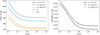 |
Fig. 11 3×2pt FoM in the optimistic scenario with and without SSC as a function of the percentage prior εb on the galaxy bias parameters for σm = (5, 50, 500) × 10−4 (solid, dashed, dotted lines). Left: FoM values. Right. ℛ(FoM), defined as the ratio between the blue and red curves. |
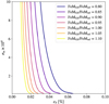 |
Fig. 12 FoMGS contours in the (εb, σm) plane for FoMGS/FoMref going from 0.8 to 1.1 in steps of 0.05 (from right to left). |
6 Conclusions
Precision cosmology requires precision computation: previously neglected theoretical contributions must therefore now be taken into account. Motivated by this consideration, we computed and studied the impact of SSC on the Euclid photometric survey, exploring how the different probes and their combination are affected by this additional, non-Gaussian term in the covariance matrix. The analysis of the impact of SSC on the spectroscopic survey, which has been shown to be small in Wadekar et al. (2020) for the Baryon Oscillation Spectroscopic Survey (BOSS) data, is left for future work. We employed a FM analysis, producing forecasts of the 1σ marginalised uncertainties on the measurement of the cosmological parameters of the flat and non-flat w0waCDM cosmological models. We validated two different forecast pipelines against the results of EC20, taking as reference survey the one specified therein, and then updated the galaxy bias and the source redshift distributions according to the most recent versions presented in Euclid Collaboration (2021). The SSC was computed relying on the analytical approximations and numerical routines presented in LG19, interfacing the public code PySSC with two distinct forecast pipelines to validate the constraints. As a further step forward, we build upon the work of LG19 by computing the scale and redshift dependence of the response functions of the different probes, starting from the results of Wagner et al. (2015b) and Barreira et al. (2018b).
We quantify the severity of the impact with the ratio σGS/σG between the marginalised or conditional uncertainties with and without SSC; this is found to vary significantly between different parameters and probes, and between the number and type of free nuisance parameters, in agreement with recent results (Upham et al. 2022; Barreira et al. 2018a; Lacasa 2020).
The conditional uncertainties show WL to be dramatically impacted by SSC, with all cosmological parameter uncertainties increasing by up to 210% (for Ωm,0) in the optimistic case. The GCph constraints are less sensitive to the addition of SSC, showing a smaller broadening of the uncertainties for all parameters, namely by up to one order of magnitude with respect to WL. The 3×2pt case sits in between these two, while being in general closer to the GCph results because of its larger constraining power.
When considering marginalised constraints, the relative impact of SSC decreases significantly. In this case, the most impacted parameters for the single probes are mainly Ωm,0, w0, wa, and σ8. Furthermore, the 3×2pt becomes by far the most impacted probe, precisely because of its power in breaking parameter degeneracies. Indeed, in the reference case and the optimistic scenario, (FoMw0wa,  ) decrease by (58%, 41%), hinting at the necessity to include SSC in the upcoming Euclid analysis.
These results are the consequence of a complicated interplay between three factors. First, SSC originates from the uncertainty in the determination of the background mean density when measuring it over a finite region. This prevents determination of the overall amplitude of the matter power spectrum, which increases the uncertainty on those parameters that concur in setting its amplitude, mainly Ωm,0 and σ8. Second, the elements of the SSC matrix depend on the amplitude of the response functions. Third, the impact depends on how large a contribution the signal receives from the low-z region, where the effective volume probed is smaller, making the variance of the background modes larger. The last two factors are both more severe for WL than for GCph, causing the former probe to be more affected than the latter.
Finally, the deviation of a given element of the GS FM from the Gaussian one also depends on its correlations: in other words, the degradation of the constraints on a given parameter can be large if this is strongly correlated with a parameter severely degraded by SSC. Quantifying the impact of SSC on a single parameter is therefore quite hard in general, and must be investigated on a case-by-case basis taking care of the details of the probe and the way it depends on the parameter of interest.
Nuisance parameters to be marginalised over act as a sort of additional contribution to the covariance. As such, the importance of both the Gaussian and SSC contribution to the overall effective covariance becomes less important when the number of nuisance parameters increases. In order to consider cases that most closely mimic future Euclid data, we opened up the parameter space by adding ΩDE,0 (i.e. removing the flatness prior). We find that, as long as the additional parameters have a scale-independent degeneracy with the most impacted ones, the relative impact of SSC decreases. We stress, however, that this reduction in the SSC impact has undesired consequences; the marginalised uncertainties on the parameters are definitely worsened, but the degradation is roughly the same whether the SSC is included or not, hence making the ratio σGS/σG closer to unity for all parameters and probes. This result can be taken as a warning against investing too much effort in refining the estimate of the computationally expensive SSC when no approximations are made. For a Euclid-like survey, the main concern would indeed be the number of nuisance parameters, which makes the impact of the SSC itself less relevant.
We furthermore note that, in light of the recent theoretical developments presented in Lacasa et al. (2023), it appears feasible to include the effect of SSC in the form of nuisance parameters, which would be the value of the density background δb in each redshift bin. This approach is interesting as it would reduce the complexity of the data covariance matrix and would allow a simpler interpretation of the effect of SSC and how it is correlated to the other cosmological and nuisance parameters.
Variations in the z binning strategy have contrasting effects: a larger number of bins means a larger number of nuisance parameters (either galaxy bias or multiplicative shear bias for each bin), which leads to a loss of constraining power. Moreover, the larger the number of bins, the larger the Gaussian contribution to the covariance, making the shot and shape noise dominate over SSC for diagonal elements. On the downside, a larger number of bins leads to larger data vectors, thus adding information that can partially compensate for the increase in the covariance. The contrasting effects at play conspire in such a way that the degradation of the FoM due to SSC is found to be approximately independent of the number of redshift bins (cfr. Fig. 10).
An interesting development in this sense is to leverage the SSC dependence on the low-z contribution to investigate whether or not its impact could be mitigated by the use of the BNT transform, which transforms redshift bins in such a way as to increase the separation between the WL kernels. This will be investigated in a forthcoming work.
An alternative strategy is to increase the constraining power by adding information through informative priors, hence recovering the FoM when SSC is incorrectly neglected. We investigate this possibility by quantifying the requirements on the prior information needed to recover the Gaussian FoM. Our results show that the main role is played here by the priors on galaxy bias parameters, while the FoM recovery is less sensitive to the prior on the multiplicative shear bias. However, the galaxy bias must be known to subpercent level in order to recover ~70% of the Gaussian FoM. Investigating whether or not this is possible is outside the scope of this paper. We nevertheless note that such remarkable prior information is the same as stating we are able to model the evolution of the bias with redshift. This is actually quite difficult based on the current knowledge of galaxy formation processes. Alternatively, one could look for an empirical fitting formula as a compromise between the need for strong priors on bias and the number of nuisance parameters.
One part of the covariance modelling not investigated in this work is the geometry of the survey footprint. While it is true that, for the large sky coverage considered, the full-sky approximation for SSC has been shown to suffice (Gouyou Beauchamps et al. 2022), a more realistic treatment accounting for the survey geometry should be considered for the Gaussian term. Still, we expect the main conclusions of this study to hold, as the mode coupling caused by the convolution with the survey mask, generating off-diagonal elements also in the Gaussian covariance, will mainly affect large scales where SSC is subdominant. It is however important to note that small holes in the survey mask (e.g. due to the presence of bright stars) generate mode coupling also on small scales, where we have seen the SSC impact to be most prominent. This will be investigated in future works.
Although some more work is needed to improve the robustness of our results, for example by comparing the different approximations presented in the literature, we can conclude that the effect of including the SSC term in the total covariance matrix of Euclid photometric observables is definitely nonnegligible, especially for WL and 3×2pt. However, the degradation of the constraints on cosmological parameters depends on the particular probe and the number and kind of parameters to constrain. The FoM is nevertheless reduced by 52% (45%) for the 3×2pt probe in the pessimistic (optimistic) scenario where all cosmological (including ΩDE,0) and nuisance (multiplicative shear bias) parameters are left free to vary. Maximising the power of the actual Euclid photometric data by taking into account the presence of SSC is a daunting task, which we will report on in a forthcoming publication.
Acknowledgements
The computational part of the work has been performed using the Python programming language, interfaced with scientific packages like astropy (Astropy Collaboration 2013, 2018) for cosmological calculations, Numba (Lam et al. 2015) for code speedup, NumPy (Harris et al. 2020) for matrix manipulation, SciPy (Virtanen et al. 2020) for numerical integration and Matplotlib (Hunter 2007) for data visualisation. The authors thank the anonymous referees for their helpful comments that improved the quality of the manuscript. DS would like to thank Raphael Kou for the fruitful discussion on the SSC impact on GCph. SGB was supported by CNES, focused on Euclid mission. The project leading to this publication has received funding from Excellence Initiative of Aix-Marseille University -A*MIDEX, a French “Investissements d’Avenir” programme (AMX-19-IET-008-IPhU). SC acknowledges support from the ‘Departments of Excellence 2018-2022’ Grant (L. 232/2016) awarded by the Italian Ministry of University and Research (MUR). IT acknowledges funding from the European Research Council (ERC) under the European Union’s Horizon 2020 research and innovation programme (Grant agreement No. 863929; project title “Testing the law of gravity with novel large-scale structure observables” and acknowledges support from the Spanish Ministry of Science, Innovation and Universities through grant ESP2017-89838, and the H2020 programme of the European Commission through grant 776247. The Euclid Consortium acknowledges the European Space Agency and a number of agencies and institutes that have supported the development of Euclid, in particular the Agenzia Spaziale Italiana, the Austrian Forschungsförderungsgesellschaft funded through BMK, the Belgian Science Policy, the Canadian Euclid Consortium, the Deutsches Zentrum für Luft- und Raumfahrt, the DTU Space and the Niels Bohr Institute in Denmark, the French Centre National d’Etudes Spatiales, the Fundação para a Ciência e a Tecnologia, the Hungarian Academy of Sciences, the Ministerio de Ciencia, Innovación y Universidades, the National Aeronautics and Space Administration, the National Astronomical Observatory of Japan, the Netherlandse Onderzoekschool Voor Astronomie, the Norwegian Space Agency, the Research Council of Finland, the Romanian Space Agency, the State Secretariat for Education, Research, and Innovation (SERI) at the Swiss Space Office (SSO), and the United Kingdom Space Agency. A complete and detailed list is available on the Euclid web site (www.euclid-ec.org).
Appendix A Details of the code validation
In the following, we provide an overview of the steps undertaken to compare and validate the codes used in this work, and some of the lessons learnt in the process.
In order to compute and validate the results we adopt the scheme sketched in Fig. A.1, which highlights the dependency of each main element of the forecast computation on the others. In particular, we have that:
The lσ constraints are obtained from the FM through Eq. (50), and the FM is built in turn from the (inverse) covariance matrix and the derivatives of the angular PS
 as indicated in Eq. (46).
The Gaussian covariance depends on the
 through Eq. (24) (and the noise PS, Eq. (25)). The SSC also depends on the
  , with the added contribution of the
  terms and the output of the PySSC module, the S ijkl matrix – following Eq. (10).
The
 are constructed by convolving the (non-linear) matter PS with the lensing and galaxy weight functions, as in Eq. (1). The Sijkl matrix also depends on the weight functions (see Eq. (11)), which are in fact the main external input needed by PySSC, and on the linear matter PS through the σ2(z1,z2) term (Eq. (5)). It is to be noted, however, that PySSC computes this PS internally, needing only the specification of a dictionary of cosmological parameters with which to call the Boltzmann solver CLASS through the Python wrapper classy. This means that we also have to make sure that the fiducial value of the parameters used to compute the PS of Eq. (1) are the same ones passed to PySSC (this time to compute the linear PS), in order to work with the same cosmology.
While to compute the constraints we follow the scheme from right to left, starting from the basic ingredients to arrive at the final result, the general trend of the validation is the opposite: we begin by comparing the final results, then work our way back whenever we find disagreement.
We then start the comparison from the σα. If a discrepancy larger than 10% is found, we check the quantities they depend on, which in this case are the covariance matrices (see Eq. (46)). If these agree, we check the codes directly. If these disagree, we iterate the process by checking the subsequent element in the scheme (in this case the Sijkl matrix and the  , until agreement is found. Essentially, this means that the disagreement in the outputs of the codes at each step can either come from the inputs, or from the codes themselves. Once the cause of the discrepancy is found and fixed, the computation is repeated and the process can start again.
The pipelines under comparison are both written in the Python language. One of them requires as external inputs the weight functions, the angular  and their derivatives with respect to the cosmological parameters; whilst the other produces these through the use of CosmoSIS14 (Jennings et al. 2016), and hence needs no external inputs but the vectors of fiducial cosmological and nuisance parameters. For the reader wishing to repeat the validation, we list below some of the lessons learnt in the code comparison process.
PySSC needs as input the WL and GCph kernels of Eqs. (18) and (21), as well as their argument, the redshift values. The code then uses this redshift array to perform the necessary integrals in dV through Simpson’s rule. The user is responsible for sampling the kernels on a sufficiently fine z grid [O(104) values have been found to be sufficient in the present case] to make sure these integrals are performed accurately.
The latest version of PySSC accepts a convention parameter. This specifies whether the kernels are in the form used in LG19 (convention = 0) or the one prescribed in EC20 (convention = 1). The two differ by a l/r2(z) factor, as shown in Eq. (23). Passing the kernels in the EC20 form without changing the parameter’s value from 0 – the default – to 1 will obviously yield incorrect results.
The ordering of the Sijkl matrix’s elements depends on the ordering chosen when passing the input kernels to PySSC – whether
 first and
  second or vice versa. This must be kept in mind when implementing Eq. (10).
The GCph constraints can show a discrepancy greater the 10% for the dark energy equation of state parameters w0 and wa even when the corresponding covariance is found to be in good agreement. This discrepancy is due to GCph being less numerically stable because of the lower constraining power compared to the other probes, and because the bias model considered has a strong degeneracy with σ8, making the numerical derivatives unstable (see e.g. Casas et al. 2023). Since this is a known issue, not coming from the SSC computation, and the covariance matrices and angular PS show good agreement, we choose to overcome the problem by using, for GCph, one code to compute both sets of parameter constraints (that is, we run one FM evaluation code with as input the covariance matrices from both groups).
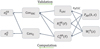 |
Fig. A.1 Some of the most important elements examined in the comparison. The arrows show the ordering followed to produce the parameters constraints, which is opposite to the one followed to validate the code. The derivatives of the PS with respect to the cosmological parameters, entering the final step of the computation, are not shown. |
Appendix B High order bias from halo model
As described in Sect. 3.6.1, the higher-order bias b(2)(z) has been estimated using the halo model. In the following, we provide further details on the input quantities, and how we set the relevant parameters.
A key role is played by the halo mass function ΦMF(M, z), which we model as
 (B.1)
(B.1)
with M the halo mass,  the mean matter density, v = δc/σ(M,z), δc = 1.686 the critical overdensity for collapse, and σ(M, z) the variance of linear perturbation smoothed with a top-hat filter of radius
 ![Mathematical equation: $R = {\left[ {3M/\left( {4\pi {{\bar \rho }_{\rm{m}}}} \right)} \right]^{1/3}}$](/articles/aa/full_html/2024/11/aa48389-23/aa48389-23-eq145.png) . We follow Tinker et al. (2010), setting
. We follow Tinker et al. (2010), setting
![Mathematical equation: $f(v) = {{\cal N}_{{\rm{MF}}}}\left[ {1 + {{\left( {{\beta _{{\rm{MF}}}}v} \right)}^{ - 2{\phi _{{\rm{MF}}}}}}} \right]{v^{2{{\rm{M}}_{{\rm{MF}}}}}}\exp \left( { - {\gamma _{{\rm{MF}}}}{v^2}/2} \right),$](/articles/aa/full_html/2024/11/aa48389-23/aa48389-23-eq146.png) (B.2)
(B.2)
where NMF is a normalisation constant, and the halo mass function fitting parameters βMF, ηMF,γMF and ϕMF – not to be confused with ΦMF(M, z) – scale with redshift as illustrated in Eqs. (9–13) of the above-mentioned paper.
The other quantity needed is the average number of galaxies hosted by a halo of mass M at redshift z. This is given by
![Mathematical equation: $\langle N\mid M\rangle (M) = {N_{{\rm{cen}}}}(M)\left[ {1 + {N_{{\rm{sat}}}}(M)} \right],$](/articles/aa/full_html/2024/11/aa48389-23/aa48389-23-eq147.png) (B.3)
(B.3)
where Nceπ(M, z) and Nsat(M, z) account for the contributions of central and satellite galaxies, respectively. We model these terms as in White et al. (2011)
![Mathematical equation: ${N_{{\rm{cen}}}}(M) = {1 \over 2}\left\{ {1 + {\mathop{\rm erfc}\nolimits} \left[ {{{\ln \left( {M/{M_{{\rm{cut}}}}} \right)} \over {\sqrt 2 {\sigma _c}}}} \right]} \right\},$](/articles/aa/full_html/2024/11/aa48389-23/aa48389-23-eq148.png) (B.4)
(B.4)
 (B.5)
(B.5)
with fiducial parameter values
 (B.6)
(B.6)
M⊙ being the mass of the Sun. These values give the best fit to the clustering of massive galaxies at z ~ 0.5 as measured from the first semester of BOSS data. It is, however, expected that they are redshift-dependent although the precise scaling with z also depends on the galaxy population used as a tracer. We therefore adjust them so that the predicted galaxy bias matches, at each given redshift, our measured values from the Flagship simulation. Since, for each z, we have a single observable quantity, we cannot fit all parameters. On the contrary, we fix all of them but Mcut to their fiducial values and use Eq. (43) to compute the bias as a function of Mcut. We then solve with respect to Mcut repeating this procedure for each redshift bin. We then linearly interpolate these values to get Mcut as a function of z, and use it to compute b(2)(z). Although quite crude, we have verified that changing the HOD parameter to be adjusted (e.g. using σc or M1) has a negligible impact on the predicted Rgm(ℓ) and Rgg(ℓ).
Appendix C Multipole binning
We bin the ℓ space according to the following procedure: the ℓk values, where k = 1,…,𝒩ℓ, are the centres of 𝒩ℓ + 1 logarithmically equispaced values, λk, which act as the edges of the 𝒩ℓ bins:
![Mathematical equation: ${\ell _k} = {\mathop{\rm dex}\nolimits} \left[ {\left( {\lambda _k^ - + \lambda _k^ + } \right)/2} \right],$](/articles/aa/full_html/2024/11/aa48389-23/aa48389-23-eq151.png) (C.1)
(C.1)
with dex(x) = 10x, = (λk,λk+1), and
 (C.2)
(C.2)
being
 (C.3)
(C.3)
In order to compute the Gaussian covariance, we also need the width of the bin, which will simply be
 (C.4)
(C.4)
so that ∆ℓk is not the same for all bins, since the bins are logarithmically – and not linearly – equispaced.
References
- Abbott, T. M. C., Abdalla, F. B., Alarcon, A., et al. 2018, Phys. Rev. D, 98, 043526 [NASA ADS] [CrossRef] [Google Scholar]
- Abbott, T. M. C., Aguena, M., Alarcon, A., et al. 2022, Phys. Rev. D, 105, 023520 [CrossRef] [Google Scholar]
- Albrecht, A., Bernstein, G., Cahn, R., et al. 2006, arXiv e-prints [arXiv:astro-ph/0609591] [Google Scholar]
- Astropy Collaboration (Robitaille, T. P., et al.) 2013, A&A, 558, A33 [NASA ADS] [CrossRef] [EDP Sciences] [Google Scholar]
- Astropy Collaboration (Price-Whelan, A. M., et al.) 2018, AJ, 156, 123 [Google Scholar]
- Barreira, A., & Schmidt, F. 2017, J. Cosmology Astropart. Phys., 06, 053 [CrossRef] [Google Scholar]
- Barreira, A., Krause, E., & Schmidt, F. 2018a, J. Cosmology Astropart. Phys., 10, 053 [CrossRef] [Google Scholar]
- Barreira, A., Krause, E., & Schmidt, F. 2018b, J. Cosmology Astropart. Phys., 06, 015 [CrossRef] [Google Scholar]
- Barreira, A., Nelson, D., Pillepich, A., et al. 2019, MNRAS, 488, 2079 [NASA ADS] [CrossRef] [Google Scholar]
- Barreira, A., Lazeyras, T., & Schmidt, F. 2021, J. Cosmology Astropart. Phys., 08, 029 [CrossRef] [Google Scholar]
- Bayer, A. E., Liu, J., Terasawa, R., et al. 2023, Phys. Rev. D, 108, 043521 [NASA ADS] [CrossRef] [Google Scholar]
- Bernardeau, F., Nishimichi, T., & Taruya, A. 2014, MNRAS, 445, 1526 [Google Scholar]
- Bird, S., Viel, M., & Haehnelt, M. G. 2012, MNRAS, 420, 2551 [Google Scholar]
- Blas, D., Lesgourgues, J., & Tram, T. 2011, J. Cosmology Astropart. Phys., 07, 034 [CrossRef] [Google Scholar]
- Casas, S., Cardone, V. F., Sapone, D., et al. 2023, A&A, submitted [arXiv:2306.1103] [Google Scholar]
- Chevallier, M., & Polarski, D. 2001, Int. J. Mod. Phys. D, 10, 213 [Google Scholar]
- Chisari, N. E., Alonso, D., Krause, E., et al. 2019, ApJS, 242, 2 [Google Scholar]
- Coe, D. 2009, arXiv e-prints [arXiv:0906.4123] [Google Scholar]
- Cragg, C., Duncan, C. A. J., Miller, L., & Alonso, D. 2023, MNRAS, 518, 4909 [Google Scholar]
- Crocce, M., Ross, A. J., Sevilla-Noarbe, I., et al. 2019, MNRAS, 482, 2807 [NASA ADS] [CrossRef] [Google Scholar]
- Desjacques, V., Jeong, D., & Schmidt, F. 2018, Phys. Rep., 733, 1 [Google Scholar]
- De Vicente, J., Sánchez, E., & Sevilla-Noarbe, I. 2016, MNRAS, 459, 3078 [NASA ADS] [CrossRef] [Google Scholar]
- Digman, M. C., McEwen, J. E., & Hirata, C. M. 2019, J. Cosmology Astropart. Phys., 10, 004 [CrossRef] [Google Scholar]
- Esteban, I., Gonzalez-Garcia, M. C., Maltoni, M., Schwetz, T., & Zhou, A. 2020, JHEP, 09, 178 [CrossRef] [Google Scholar]
- Euclid Collaboration (Martinet, N., et al.) 2019, A&A, 627, A59 [NASA ADS] [CrossRef] [EDP Sciences] [Google Scholar]
- Euclid Collaboration (Blanchard, A., et al.) 2020, A&A, 642, A191 [NASA ADS] [CrossRef] [EDP Sciences] [Google Scholar]
- Euclid Collaboration (Pocino, A., et al.) 2021, A&A, 655, A44 [NASA ADS] [CrossRef] [EDP Sciences] [Google Scholar]
- Euclid Collaboration (Mellier, Y., et al.) 2024, A&A, in press, https://doi.org/18.1851/8884-6361/282458818 [Google Scholar]
- Gouyou Beauchamps, S., Lacasa, F., Tutusaus, I., et al. 2022, A&A, 659, A128 [NASA ADS] [CrossRef] [EDP Sciences] [Google Scholar]
- Hamilton, A. J. S., Rimes, C. D., & Scoccimarro, R. 2006, MNRAS, 371, 1188 [Google Scholar]
- Harris, C. R., Millman, K. J., van der Walt, S. J., et al. 2020, Nature, 585, 357 [NASA ADS] [CrossRef] [Google Scholar]
- Hoyle, B., Gruen, D., Bernstein, G. M., et al. 2018, MNRAS, 478, 592 [Google Scholar]
- Hu, W., & Kravtsov, A. V. 2003, ApJ, 584, 702 [Google Scholar]
- Hu, W., & Jain, B. 2004, Phys. Rev. D, 70, 043009 [Google Scholar]
- Hunter, J. D. 2007, Comput. Sci. Eng., 9, 90 [NASA ADS] [CrossRef] [Google Scholar]
- Ivanov, M. M., Cuesta-Lazaro, C., Mishra-Sharma, S., Obuljen, A., & Toomey, M. W. 2024, arXiv e-prints [arXiv:2402.13310] [Google Scholar]
- Ivezić, Ž., Kahn, S. M., Tyson, J. A., et al. 2019, ApJ, 873, 111 [Google Scholar]
- Jennings, E., Zuntz, J., Paterno, M., et al. 2016, in Python in Astronomy 2016, eds. T. Jenness, T. Robitaille, E. Tollerud, S. Mumford, & K. Cruz, 14 [Google Scholar]
- Joachimi, B., & Bridle, S. L. 2010, A&A, 523, A1 [NASA ADS] [CrossRef] [EDP Sciences] [Google Scholar]
- Joachimi, B., Cacciato, M., Kitching, T. D., et al. 2015, Space Sci. Rev., 193, 1 [Google Scholar]
- Kaiser, N. 1998, ApJ, 498, 26 [NASA ADS] [CrossRef] [Google Scholar]
- Kilbinger, M., Heymans, C., Asgari, M., et al. 2017, MNRAS, 472, 2126 [Google Scholar]
- Kitching, T. D., Alsing, J., Heavens, A. F., et al. 2017, MNRAS, 469, 2737 [Google Scholar]
- Krause, E., & Eifler, T. 2017, MNRAS, 470, 2100 [NASA ADS] [CrossRef] [Google Scholar]
- Krause, E., Fang, X., Pandey, S., et al. 2021, arXiv e-prints [arXiv:2105.13548] [Google Scholar]
- Lacasa, F. 2020, A&A, 634, A74 [NASA ADS] [CrossRef] [EDP Sciences] [Google Scholar]
- Lacasa, F., & Grain, J. 2019, A&A, 624, A61 [NASA ADS] [CrossRef] [EDP Sciences] [Google Scholar]
- Lacasa, F., & Rosenfeld, R. 2016, J. Cosmology Astropart. Phys., 08 (2016), 005 [CrossRef] [Google Scholar]
- Lacasa, F., Lima, M., & Aguena, M. 2018, A&A, 611, A83 [NASA ADS] [CrossRef] [EDP Sciences] [Google Scholar]
- Lacasa, F., Aubert, M., Baratta, P., et al. 2023, A&A, 671, A115 [NASA ADS] [CrossRef] [EDP Sciences] [Google Scholar]
- Lam, S. K., Pitrou, A., & Seibert, S. 2015, in Proc. Second Workshop on the LLVM Compiler Infrastructure in HPC, 1 [Google Scholar]
- Laureijs, R., Amiaux, J., Arduini, S., et al. 2011, arXiv e-prints [arXiv:1110.3193] [Google Scholar]
- Lazeyras, T., Wagner, C., Baldauf, T., & Schmidt, F. 2016, J. Cosmology Astropart. Phys., 02, 018 [CrossRef] [Google Scholar]
- Lewis, A., Challinor, A., & Lasenby, A. 2000, ApJ, 538, 473 [Google Scholar]
- Li, Y., Hu, W., & Takada, M. 2014, Phys. Rev. D, 89, 083519 [NASA ADS] [CrossRef] [Google Scholar]
- Li, Y., Hu, W., & Takada, M. 2016, Phys. Rev. D, 93, 063507 [NASA ADS] [CrossRef] [Google Scholar]
- Limber, D. N. 1953, ApJ, 117, 134 [NASA ADS] [CrossRef] [Google Scholar]
- Linder, E. V. 2005, Phys. Rev. D, 72, 043529 [Google Scholar]
- Linke, L., Burger, P. A., Heydenreich, S., Porth, L., & Schneider, P. 2024, A&A, 681, A33 [NASA ADS] [CrossRef] [EDP Sciences] [Google Scholar]
- Mead, A. J., Brieden, S., Tröster, T., & Heymans, C. 2021, MNRAS, 502, 1401 [Google Scholar]
- Pandey, S., Krause, E., DeRose, J., et al. 2022, Phys. Rev. D, 106, 043520 [NASA ADS] [CrossRef] [Google Scholar]
- Perlmutter, S., Aldering, G., Goldhaber, G., et al. 1999, ApJ, 517, 565 [Google Scholar]
- Potter, D., Stadel, J., & Teyssier, R. 2017, Computat. Astrophys. Cosmol., 4, 2 [NASA ADS] [CrossRef] [Google Scholar]
- Reischke, R. 2024, MNRAS, 530, 4412 [NASA ADS] [CrossRef] [Google Scholar]
- Riess, A. G., Filippenko, A. V., Challis, P., et al. 1998, AJ, 116, 1009 [Google Scholar]
- Rimes, C. D., & Hamilton, A. J. S. 2006, MNRAS, 371, 1205 [NASA ADS] [CrossRef] [Google Scholar]
- Rizzato, M., Benabed, K., Bernardeau, F., & Lacasa, F. 2019, MNRAS, 490, 4688 [NASA ADS] [CrossRef] [Google Scholar]
- Schaan, E., Takada, M., & Spergel, D. N. 2014, Phys. Rev. D, 90, 123523 [NASA ADS] [CrossRef] [Google Scholar]
- Spergel, D., Gehrels, N., Baltay, C., et al. 2015, arXiv e-prints [arXiv: 1503.03757] [Google Scholar]
- Takada, M., & Hu, W. 2013, Phys. Rev. D, 87, 123504 [NASA ADS] [CrossRef] [Google Scholar]
- Takahashi, R., Sato, M., Nishimichi, T., Taruya, A., & Oguri, M. 2012, ApJ, 761, 152 [Google Scholar]
- Taylor, P. L., Bernardeau, F., & Kitching, T. D. 2018a, Phys. Rev. D, 98, 083514 [Google Scholar]
- Taylor, P. L., Kitching, T. D., McEwen, J. D., & Tram, T. 2018b, Phys. Rev. D, 98, 023522 [NASA ADS] [CrossRef] [Google Scholar]
- Tegmark, M., Taylor, A. N., & Heavens, A. F. 1997, ApJ, 480, 22 [NASA ADS] [CrossRef] [Google Scholar]
- Tinker, J. L., Robertson, B. E., Kravtsov, A. V., et al. 2010, ApJ, 724, 878 [NASA ADS] [CrossRef] [Google Scholar]
- Troxel, M. A., MacCrann, N., Zuntz, J., et al. 2018, Phys. Rev. D, 98, 043528 [Google Scholar]
- Tutusaus, I., Martinelli, M., Cardone, V. F., et al. 2020, A&A, 643, A70 [EDP Sciences] [Google Scholar]
- Unruh, S., Schneider, P., Hilbert, S., et al. 2020, A&A, 638, A96 [NASA ADS] [CrossRef] [EDP Sciences] [Google Scholar]
- Upham, R. E., Brown, M. L., Whittaker, L., et al. 2022, A&A, 660, A114 [NASA ADS] [CrossRef] [EDP Sciences] [Google Scholar]
- Virtanen, P., Gommers, R., Oliphant, T. E., et al. 2020, Nature Methods, 17, 261 [CrossRef] [Google Scholar]
- Voivodic, R., & Barreira, A. 2021, J. Cosmology Astropart. Phys., 05, 069 [CrossRef] [Google Scholar]
- Wadekar, D., Ivanov, M. M., & Scoccimarro, R. 2020, Phys. Rev. D, 102, 123521 [CrossRef] [Google Scholar]
- Wagner, C., Schmidt, F., Chiang, C. T., & Komatsu, E. 2015a, MNRAS, 448, L11 [CrossRef] [Google Scholar]
- Wagner, C., Schmidt, F., Chiang, C.-T., & Komatsu, E. 2015b, J. Cosmology Astropart. Phys., 08, 042 [CrossRef] [Google Scholar]
- White, M., Blanton, M., Bolton, A., et al. 2011, ApJ, 728, 126 [NASA ADS] [CrossRef] [Google Scholar]
- Yao, J., Shan, H., Li, R., et al. 2024, MNRAS, 527, 5206 [Google Scholar]
- Zennaro, M., Angulo, R. E., Contreras, S., Pellejero-Ibáñez, M., & Maion, F. 2022, MNRAS, 514, 5443 [NASA ADS] [CrossRef] [Google Scholar]
Here we do not consider a redshift dependence of  but this can happen for surveys with significant depth variations across the sky. This is discussed in Lacasa et al. (2018).
Since we are using the non-linear matter power spectrum Pmm(k, z), we do not force Rmm(k, z) to reduce to its linear expression, that is to say, we do not set  in Eq. (12).
Equation (19) assumes general relativity and a spatially flat Universe. For the general case, one must replace the term in brackets with fK(r’ − r)/fK(r′), with fK(r) the function giving the comoving angular-diameter distance in a non-flat universe.
We neglect the response of 〈N|M〉 to a perturbation δb in the background density, as done in LG19.
Available upon request to the author, Davide Sciotti.
All Tables
Ratio between the GS and G conditional uncertainties for all cosmological parameters and probes in the reference case, for the optimistic settings.
Ratio between the GS and G marginalised uncertainties for all cosmological parameters and the FoM in the reference scenario, for the optimistic and pessimistic settings.
All Figures
|
Fig. 1 Projected response coefficients for the WL and GCph probes and their cross-correlation for the central redshift bin (0.8 ≲ z ≲ 0.9). The shape and amplitude of the functions for different redshift pairs are analogous. For WL, the baryon acoustic oscillation wiggles are smoothed out by the projection, because the kernels are larger than the GCph ones. The different amplitude of the response is one of the main factors governing the severity of SSC. |
| In the text | |
|
Fig. 2 Kernels and galaxy distribution considered in this work. The first two plots show the kernels, or weight for the two photometric probes. The analytic expressions for these are, respectively, Eqs. (18) (left, WL) and (21) (right, GCph). At high redshifts, the IA term dominates over the shear term in the lensing kernels, making them negative. The rightmost plot shows the redshift distribution per redshift bin for the sources (and lenses), as well as their sum, obtained from the Flagship 1 simulation as described in Sect. 3.1. |
| In the text | |
|
Fig. 3 Correlation matrix in log scale for all the statistics of the 3×2pt data-vector in the G and GS cases. The positive and negative elements are shown in red and blue, respectively. The Gaussian covariance is block diagonal (i.e. it is diagonal in the multipole indices, but not in the redshift ones; the different diagonals appearing in the plot correspond to the different redshift pair indices, for ℓ1 = ℓ2). The overlap in the WL kernels makes the WL block in the Gaussian + SSC covariance matrix much more dense than the GCph one. |
| In the text | |
|
Fig. 4 Percentage discrepancy of the normalised 1σ uncertainties with respect to the mean for the WL probe, both in the G and GS cases (optimistic settings). The index i = A, B indicates the two pipelines, whilst α indexes the cosmological parameter. The desired agreement level is reached in all cases (WL, GCph probes and pessimistic case not shown). |
| In the text | |
|
Fig. 5 Marginalised and conditional optimistic 1σ uncertainties on the cosmological parameters, relative to their corresponding fiducial values (in percent units), in both the G and GS cases for WL, GCph, and the 3×2pt. We highlight the logarithmic scale on the x-axis, made necessary by the large range of values. The values in these plots have been used to compute the ratios in Tables 1 and 2. |
| In the text | |
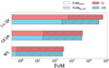 |
Fig. 6 Same as Fig. 5, but for the dark energy and Ωm,0 − S8 FoM. |
| In the text | |
|
Fig. 7 Contour plot for the G and GS constraints, considering the full 3×2pt analysis in the optimistic case, in the reference scenario. The two shaded regions of the ellipses represent the 1 and 2σ contours. For clarity, the nuisance parameters are shown separately in Fig. 8 and the log10(TAGN/K) parameter name has been shortened to log(T). |
| In the text | |
|
Fig. 8 Percent increase of the marginalised 1σ uncertainty of the nuisance parameters, for all probe choices, in the optimistic case and for the reference scenario. |
| In the text | |
|
Fig. 9 Ratio between WL and 3×2pt marginalised uncertainties computed by including or neglecting the SSC contribution, as a function of the number of (equally populated) redshift bins, for the pessimistic and optimistic cases. |
| In the text | |
|
Fig. 10 FoM ratio vs the number of EP and ED гedshift bins for WL (left) and 3×2pt (right) in the optimistic scenario. The blue curves in this plot match the ones in the bottom right panel of Fig 9 in the optimistic case, for the corresponding probes. |
| In the text | |
|
Fig. 11 3×2pt FoM in the optimistic scenario with and without SSC as a function of the percentage prior εb on the galaxy bias parameters for σm = (5, 50, 500) × 10−4 (solid, dashed, dotted lines). Left: FoM values. Right. ℛ(FoM), defined as the ratio between the blue and red curves. |
| In the text | |
|
Fig. 12 FoMGS contours in the (εb, σm) plane for FoMGS/FoMref going from 0.8 to 1.1 in steps of 0.05 (from right to left). |
| In the text | |
|
Fig. A.1 Some of the most important elements examined in the comparison. The arrows show the ordering followed to produce the parameters constraints, which is opposite to the one followed to validate the code. The derivatives of the PS with respect to the cosmological parameters, entering the final step of the computation, are not shown. |
| In the text | |
Current usage metrics show cumulative count of Article Views (full-text article views including HTML views, PDF and ePub downloads, according to the available data) and Abstracts Views on Vision4Press platform.
Data correspond to usage on the plateform after 2015. The current usage metrics is available 48-96 hours after online publication and is updated daily on week days.
Initial download of the metrics may take a while.