© The Authors 2024

1 Introduction

In recent decades, a large number of observations and studies have been converging on the fact that our Universe is going through a phase of accelerated expansion, visible on cosmo-logical scales. In order to better understand the origin of this cosmic acceleration and the physics of gravity on large scales, wide galaxy surveys such as Euclid¹ (Laureijs et al. 2011; Euclid Collaboration 2024c) rely essentially on two main probes: galaxy clustering, denoted here by GC_sp (GC_ph) for analyses with spectroscopic (photometric) redshifts; and weak gravitational lensing (WL), also known as cosmic shear. The GC_sp and GC_ph probes aim at reconstructing the fluctuations of the underlying dark matter density using coordinates and redshifts from the angular and radial positions of galaxies. Different measurements can be done to extract information from this underlying distribution, such as measurements of the baryon acoustic oscillations (BAOs; Eisenstein et al. 2005; Aubourg et al. 2015), or measurements of the redshift-space distortion effects (RSD; Percival & White 2009). Complementary to the clustering probes, galaxy surveys enable WL analyses. They characterise the matter present along the line of sight, which slightly alters the images of galaxies as a function of the gravitational potentials traversed by photons (see, e.g., Kilbinger 2015, for a detailed review). WL analyses not only extract information about the matter content of the Universe, but also about the growth ofstructure and the physics of gravitational interaction. Stage-IV galaxy surveys, such as Euclid, will provide a large amount of data that will enable very precise GC_sp, GC_ph, and WL analyses (see, e.g., Euclid Collaboration 2020, from hereafter EP:VII).

Euclid is an ESA M-class space mission whose main goal is to measure the geometry of the Universe and the growth of structures out to redshift z ~ 2, i.e., a look-back time of 10Gyr and beyond. This space telescope, launched on 1st July 2023, carries a near-infrared spectrometer and photometer instrument (Maciaszek et al. 2022; Euclid Collaboration 2024b, Euclid-NISP) and a visible imager (Cropper et al. 2018; Euclid Collaboration 2024a, Euclid-VIS). These two detectors will perform a galaxy survey over an area of about 15 000 deg² of the extragalactic sky. Euclid-NISP will be able to measure 30 to 50 million spectroscopic redshifts between 0.9 and 1.8 (Pozzetti et al. 2016), which can be used for GC measurements, while Euclid-VIS will measure about 1.5 billion photometric galaxy shapes, enabling WL observations (see Laureijs et al. 2011, for more details). The huge volume of data provided by Euclid will give newinsights into the late Universe, especially on the growth and evolution of large-scale cosmic structures and on the expansion history of the Universe, and more generally shed some light on the nature of dark energy (see Amendola et al. 2018).

As shown in EP:VII, the combination of all main probes (GC_sp, GC_ph, and WL) will lead to the most stringent constraints from future Euclid data. The combination of different probes, sensitive to different aspects of how gravity acts in the cosmos, breaks several degeneracies present between the different cosmological parameters and achieves better constraints.

However, such cosmological probes are in general not independent. It was shown in EP:VII that the cross-correlations between GC_ph and WL were another important key contributor in the joint analysis of all Euclid probes. More precisely, the figure-of-merit (FoM, Albrecht et al. 2006) of the dark energy equation-of-state parameters improves roughly by a factor of 4 when these cross-correlations are included in the analysis. It was also shown in Tutusaus et al. (2020) that a joint analysis of Euclid photometric probes accounting for their cross-correlations can significantly improve our knowledge on nuisance parameters, such as the intrinsic alignment of galaxies or the galaxy bias. Cross-correlations between GC_ph and WL have been studied for real observations (see, e.g., Abbott et al. 2022) and the future Euclid data (Tutusaus et al. 2020). Similarly, there have been several analysis combining spectroscopic and photometric data (see, e.g., Heymans et al. 2021; Sugiyama et al. 2023). However, the full treatment of all cross-correlations between the spectroscopic probe, GC_sp, and the photometric probes, taking into account their covariances and the radial information, has been less considered. One of the main reasons is that spectroscopic analyses are usually performed in three-dimensions, while photometric analyses are done in two-dimensions. This difference makes it non-trivial to properly combine the spectroscopic and photometric probes while accounting for their cross-correlations (although several attempts are available in the literature, see, e.g., Passaglia et al. 2017; Wang et al. 2020; Taylor & Markovič 2022). In EP:VII, the authors neglected any correlation between GC_sp and the photometric probes. In the case of Euclid, another motivation for this choice is that the spectroscopic measurements will be available only at high redshift (z > 0.9), therefore reducing their overlap in volume with the photometric probes. In order to be conservative, a pessimistic scenario was further considered in EP:VII where all objects above z = 0.9 were removed for GCph (and their cross-correlations with WL), with the goal of removing any remaining correlation.

In the present analysis we go beyond the results presented in EP:VII by focusing on extracting additional information from the combination of spectroscopic and photometric probes. Without accounting for all the cross-correlations between spectroscopic and photometric observables (which would require a joint modelling of three- and two-dimensional probes), we extract the additional information from the fact that GC_sp and GC_ph will probe (at least partially) the same volume of the Universe.

To do so, we introduce the ratio of angular correlation functions (or harmonic space power spectra) between the spectroscopic and photometric tracers as an additional observable according to Alimi et al. (1988) who first suggested this type of statistic to get rid of sampling variance. Indeed, given the large number density of Euclid objects, if tracers are accurately selected we can get rid of the cosmic variance and obtain very precise measurements of these ratios. In practice, this implies that once the bias of one tracer is determined, there is effectively almost no uncertainty on the bias of the other tracer. This approach made it possible to implement a multi-tracer approach (Seljak 2009; McDonald & Seljak 2009). This principle of this method has been extensively investigated and it has been applied in a few cases. Recent short reviews can be found in Wang & Zhao (2020); Blanchard (2022). Given the reduction in the effective number of degrees of freedom, it is natural to expect an improvement in the constraints. As we will see in the following, this method can significantly enhance the forecasted Euclid constraints: it leads to an improvement of the FoM ranging from 5% up to 60%, compared to the baseline analysis presented in EP:VII. The specific improvement depends on the settings of the surveys and the cosmological model considered.

The paper is organised as follows. We first describe the Euclid survey and how we forecast its constraining power for the main cosmological probes in Sect. 2. We then present the cosmological models considered in Sect. 3. In Sect. 4 we introduce our new observable making use of the multi-tracer approach, and clarify in Sect. 5 its implementation in our forecasts. The main results of the analysis are presented in Sect. 6, and we conclude in Sect. 7.

2 The main Euclid cosmological probes

In this section we describe how we forecast the constraining power of Euclid for its main cosmological probes. We follow closely the recipes presented in EP:VII and, although we provide a self-contained description in this work, we refer the interested reader to EP:VII for all the technical details.

2.1 Spectroscopic probe

Let us first consider the spectroscopic probe of Euclid. The main observable for this probe is the observed galaxy power spectrum, which needs a reference cosmology. Following EP:VII we model it as $$\begin{array}{cc}{P}_{\text{obs}}\left(k_{\text{ref}},{\mu }_{\text{ref}};z\right)=& \frac{1}{q_{\perp }^2(z)q_{\left|\right|}(z)}\left\{\frac{{\left[b_{\text{sp}}{\sigma }_8(z)+f{\sigma }_8(z){\mu }^2\right]}^2}{1+{\left[f(z)k\mu {\sigma }_{\text{p}}(z)\right]}^2}\right\}\hfill \\ & \times \frac{P_{\text{dw}}(k,\mu ;z)}{{\sigma }_8^2(z)}{F}_z(k,\mu ;z)+P_{\text{s}}(z),\hfill \end{array}$$(1)

where σ₈ is the r.m.s. of linear matter fluctuations on scales of 8 h^–1Mpc, b_sp the galaxy bias parameter, f the growth rate, σ_p is related to the pairwise peculiar velocity and treated as a free nuisance parameter, µ the cosine of the angle between the wave vector, k, and the line-of-sight direction, and all k : = k(k^ref,µ_ref) and µ := µ(µ_ref) with $$k\left(k_{\text{ref}},{\mu }_{\text{ref}}\right)=\frac{k_{\text{ref}}}{q_{\perp }}{\left[1+{\mu }_{\text{ref}}^2\left(\frac{q_{\perp }^2}{q_{\left|\right|}^2}-1\right)\right]}^{1/2},$$(2) $$\mu \left({\mu }_{\text{ref}}\right)={\mu }_{\text{ref}}\frac{q_{\perp }}{q_{\left|\right|}}{\left[1+{\mu }_{\text{ref}}^2\left(\frac{q_{\perp }^2}{q_{\left|\right|}^2}-1\right)\right]}^{1/2}.$$(3)

RSDs are accounted for through the numerator inside the curly bracket in Eq. (1), and the ‘finger-of-God’ effect through the denominator. The term P_dw is the ’de-wiggled’ power spectrum, which accounts for the smearing of the BAOs: $$P_{\text{dw}}(k,\mu ;z)=P_{\delta \delta }^{lin}(k;z){\text{e}}^{-g_{\mu }{k}^2}+P_{\text{nw}}(k;z)\left(1-{\text{e}}^{-g_{\mu }{k}^2}\right),$$(4)

where P_nw stands for a no-wiggle power spectrum with the same broad band shape as the linear power spectrum, $P_{\delta \delta }^{\lim }$, but without the BAO wiggles. We also account for nonlinearities through a nonlinear damping factor $$g_{\mu }(k,\mu ,z)={\sigma }_v^2(z)\left\{1-{\mu }^2+{\mu }^2{[1+f(z)]}^2\right\},$$(5)

with $${\sigma }_{\text{v}}^2(z)=\frac{1}{6{\pi }^2}{\displaystyle {\int }_0^{+\infty }\text{d}}k{P}_{\delta \delta }^{\mathrm{lin}}(k,z).$$(6)

We additionally introduce $$F_z(k,\mu ;z)={\text{e}}^{-k^2{\mu }^2{\sigma }_r^2(z)},$$(7)

where σr(z) = (1 + z)σ_zc/H(z) accounts for redshift uncertainties and is modelled as in EP:VII. We set σ_z = 10^–3 (corresponding to the required precision on spectroscopic redshift in Euclid). Moreover, we consider a residual shot-noise P_s as a constant nuisance parameter in each redshift bin. Finally, the quantities $$q_{\perp }(z)=\frac{r(z)}{r_{\text{ref}}(z)},$$(8) $$q_{\left|\right|}(z)=\frac{H_{\text{ref}}(z)}{H(z)},$$(9)

account for the Alcock-Paczynski effect (Alcock & Paczynski 1979), where r(z) stands for the comoving angular distance and H(z) is the Hubble expansion rate. The quantities indexed by ‘ref’ refer to the quantities in the reference cosmology required for measurements of the power spectrum in the spectroscopic survey.

2.2 Photometric probes

With respect to the photometric survey, we consider the harmonic-space angular power spectra $C_{ij}^{XY}(\ell )$, with i and j representing two tomographic bins, and X and Y being either GC_ph or WL. Under the extended Limber approximation (LoVerde & Afshordi 2008), these are given by $$C_{ij}^{XY}(\ell )=c{\displaystyle {\int }_{z_{\min }}^{z_{\max }}\text{d}}z\frac{W_i^X(z)W_j^Y(z)}{H(z)r^2(z)}{P}_{\delta \delta }\left(k_{\ell },z\right),$$(10)

where k_ℓ = (ℓ + 1/2)/r(z), and the nonlinear matter power spectrum is represented by P_δδ.

The remaining ingredients in Eq. (10) are the kernels for GCph or WL, $$W_i^{{\text{GC}}_{\text{ph}}}(z)=b_i^{\text{ph}}(z)n_i(z)\frac{H(z)}{c},$$(11) $$\begin{array}{l}{W}_i^{\text{WL}}(z)=\frac{3}{2}{\text{Ω}}_{\text{m},0}\frac{H_0^2}{c^2}(1+z)r(z){{{\displaystyle \int }}^{\text{}}}_z^{z_{\max }}\text{d}{z}^{\prime }{n}_i\left(z^{\prime }\right)\frac{r\left(z,z^{\prime }\right)}{r\left(z^{\prime }\right)}\hfill \\ +W_i^{\text{IA}}(z),\hfill \end{array}$$(12)

with ni(z′) being the normalised number density distribution of galaxies in tomographic bin i, $b_i^{\text{ph}}(z)$ the linear galaxy bias in the same bin, and r(z, z′) the comoving angular diameter distance of a source at redshift z′ seen from an observer at redshift z. We also consider the intrinsic alignment (IA) of galaxies with the extended nonlinear alignment (eNLA) model, as in EP:VII. This corresponds to the kernel $$W_i^{\text{IA}}(k,z)=-\frac{{\mathcal{A}}_{\text{IA}}{C}_{\text{IA}}{\text{Ω}}_{\text{m},0}{ℱ}_{\text{IA}}(z)}{D(z)}\frac{H(z)}{c},$$(13)

with D the growth factor for linear perturbations: $$\delta (z)=D(z){\delta }_0,$$(14)

normalised to 1 at z = 0, and $${ℱ}_{\text{IA}}(z)={(1+z)}^{{\eta }_{\text{IA}}}{\left[\frac{\langle L\rangle (z)}{L_{*}(z)}\right]}^{{\beta }_{\text{IA}}}.$$(15)

The functions 〈L〉(z) and L_∗(z) are the redshift-dependent mean and the characteristic luminosity of source galaxies as computed from the luminosity function. For the parameters of the IA model, η_IA, β_IA, C_IA, and A_IA, we consider the fiducial values presented in EP:VII. Further details on the eNLA model and the luminosity dependence assumed can be found there.

2.3 Forecast code

In order to compute the observables described in the previous sections and forecast their constraining power on cosmological parameters, we consider here the TotallySAF² code, which relies on CAMB (Lewis et al. 2000) to solve the Boltzmann equations. TotallySAF has been used previously for forecasting the constraining power of the main cosmological probes of Euclid using the Fisher formalism (EP:VII). The same code allows us to forecast both the spectroscopic (GCsp) and photometric probes (WL and GCph), as well as their cross-correlations. An important feature of this code is the possibility to specify the number of points in the n-point stencil derivatives and therefore achieve a high level of accuracy, avoiding numerical instabilities in the Fisher forecast (Yahia-Cherif et al. 2021).

3 Cosmological models

In the present study, the cosmological models investigated are the ones described in EP:VII. These models are spatially flat universes filled with cold dark matter and dynamical dark energy. We also considered non-flat models and a modified gravity model. The dynamics of dark energy is described by a timevarying equation-of-state parameter following the popular CPL parameterisation (Chevallier & Polarski 2001; Linder 2005): $$w(z)=w_0+w_a\frac{z}{1+z}.$$(16)

Five other cosmological parameters enter in the model: the dimensionless Hubble constant h (defined by H₀ = 100h km s^–1 Mpc^–1); the total matter density at the present time Ω_m; the dark energy density at the present time Ω_DE; the current baryonic matter density Ω_b; the spectral index n_s of the primordial spectrum of scalar perturbations; and the current amplitude of matter fluctuations as expressed by σ₈ (the r.m.s. of linear matter fluctuations in spheres of 8h^-1 Mpc radius). For the description of linear matter perturbations in CAMB we take into account here the parameterised-post-Friedmann (PPF) framework of Hu & Sawicki (2007), which enables the equation- of-state to cross w(z) = –1 without developing instabilities in the perturbation sector.

Extensions of ΛCDM theories may alter the background as well as the perturbation sector. A simple way to investigate this possibility is through the growth index γ, defined as $$\gamma (z)=\frac{\ln f(z)}{\ln {\text{Ω}}_{\text{m}}(z)},\text{\hspace{0.17em}\hspace{0.17em}with\hspace{0.17em}\hspace{0.17em}}{\text{Ω}}_{\text{m}}(z)\equiv \frac{{\text{Ω}}_{\text{m},0}{(1+z)}^3{H}_0^2}{H^2(z)},$$(17)

and f (z) the growth rate, $$f(z)\equiv -\frac{\text{d\hspace{0.17em}}\ln D(z)}{\text{d\hspace{0.17em}}\ln (1+z)}.$$(18)

In standard gravity models, the growth factor is well approximated with a constant γ ≈ 0.55, having a weak dependence on Λ (Lahav et al. 1991). Introducing γ as a constant free parameter is a simple way to describe possible departures from the standard model (Linder 2003).

The fiducial case is the standard concordance model, that is, a spatially flat Universe filled mostly with cold dark matter and a cosmological constant. Our cosmological models are described by the following vector of parameters with their fiducial values coming from EP:VII: $$\begin{array}{l}\lambda =\left\{{\text{Ω}}_{\text{m},0},{\text{Ω}}_{\text{b},0},w_0,w_a,h,n_{\text{s}},{\sigma }_8,{\text{Ω}}_{\text{DE}},\gamma \right\}\hfill \\ =\{0.32,0.05,-1.0,0.0,0.67,0.96,0.816,0.68,0.55\}.\hfill \end{array}$$(19)

There are also several nuisance parameters. For the photometric sample, these include the three parameters for the intrinsic alignments, A_IA, η_IA, β_IA, and the linear galaxy bias in each tomographic bin. For the spectroscopic sample, we consider the linear galaxy bias parameter and the residual shot noise, Ps , in each redshift bin.

The sum of neutrino masses is also fixed to 0.06 eV. In the presence of massive neutrinos, the redshift and scale dependence of the linear growth factor differs from the zero-mass case. This effect is taken into account in standard Boltzmann solvers such as CAMB (Lewis et al. 2000)or CLASS (Lesgourgues 2011). However, given the small neutrino masses considered in this work, we neglect neutrino effects on the growth factor, following the same approach as in EP:VII, for simplicity.

4 The ratio of correlation functions as additional information

The ratio of the correlation functions of two different galaxy samples, also known as the ratio of cross-correlations, is a powerful method to measure the ratio of the galaxy bias of their respective populations (Alimi et al. 1988). Let us consider measuring two galaxy populations, tracers of the matter density field, δ1 and δ2 . Let us further assume that both tracers are Poisson realizations of the underlying density fields δ_i = b_iδ, with b₁, b₂ being the large-scale biases of the two tracers. When the two galaxy populations follow the same selection function over the same volume, this ratio is insensitive to the sampling variance and the Poisson noise is the only source of variance. If the selection functions are different but known, an appropriate weighting scheme will achieve the same result. This is the essence of the multi-tracer approach. It can also be applied to RSD and non- gaussianity measurements (Seljak 2009; McDonald & Seljak 2009). This approach can be applied equivalently to the angular correlation functions or the harmonic power spectra of the two galaxy samples (see for instance Tanidis & Camera 2021; Abramo et al. 2022). In the following, we will consider these two populations to be the spectroscopic and photometric populations of the galaxies observed by Euclid. However, it is important to have the same selection function in both data sets in order to benefit from the insensitivity to sample variance. Because of this, we will choose the spectroscopic sample by selecting those galaxies in each one of the photometric tomographic bins for which spectroscopic information is available. This is aimed at ensuring that the selection function for both data sets in the new observable will be the same, that is, the photometric selection function. A weighting scheme could be necessary to properly achieve this goal, which is feasible as long as the selection functions of the samples are known. To ensure that the same galaxies are not used twice, we will assume that the galaxies in the spectroscopic sample have been removed from the photometric sample.

We first denote as a_ℓm,sp (a_ℓm,ph) the coefficients of the spherical-harmonic decomposition of the spectroscopic (photometric) galaxy distribution and the corresponding angular power spectrum Cℓm,sp (Cℓm,ph).

The aℓm,sp for the spectroscopic survey can be written as ${\widehat{a}}_{\ell m,\text{sp}}=b_{\text{sp}}{a}_{\ell m}^{\text{DM}}+a_{\ell m,\text{sp}}^P$ , where b_sp represents the spectroscopic bias, assumed to be a constant (i.e., no stochasticity in the bias) $a_{\ell m}^{\text{DM}}$ denotes the contribution from the matter distribution, and finally $a_{\ell m,\text{sp}}^p$ represents the contribution from the Poisson noise. The Poisson noise is characterized by $\langle a_{\ell m,\text{sp}}^p\rangle =0$ and $\langle {\left|a_{\ell m,\text{sp}}^p\right|}^2\rangle =\frac{1}{n_{\text{sp}}}$. The estimator of the angular power spectrum is given by: $$\begin{array}{ll}{\widehat{C}}_{\ell ,\text{sp}}\hfill & =\frac{1}{2\ell +1}{\displaystyle {\displaystyle \sum }_m}{\left|{\widehat{a}}_{\ell m,\text{sp}}\right|}^2\hfill \\ \hfill & =\frac{1}{2\ell +1}{\displaystyle {\displaystyle \sum }_m}\left(b_{\text{sp}}^2{\left|a_{\ell m}^{\text{DM}}\right|}^2+2b_{\text{sp}}\mathrm{Re}\left(a_{\ell m}^{\text{DM}}{a}_{\ell m}^{p\ast }\right)+{\left|a_{\ell m}^p\right|}^2\right).\hfill \end{array}$$(20)

The average over Poisson realization yields $$\langle {\widehat{C}}_{\ell ,\text{sp}}\rangle =\frac{1}{2\ell +1}{\displaystyle \sum _m{b}_{\text{sp}}^2}{\left|a_{\ell m}^{\text{DM}}\right|}^2+\frac{1}{n_{\text{sp}}}={\overline{C}}_{\ell ,\text{sp}}+\frac{1}{n_{\text{sp}}}.$$(21)

Here, the quantity ${\overline{C}}_{\ell ,\text{sp}}$ is the angular power spectrum of the dark matter component in the survey area. For the photometric survey, similar expressions can be formulated, with the Poisson noise being negligible due to a significantly larger n_ph compared to n_sp. Consequently, for the photometric angular power spectrum, we have $$\langle {\widehat{C}}_{\ell ,\text{ph}}\rangle \simeq {\overline{C}}_{\ell ,\text{ph}}=\frac{1}{2\ell +1}{\displaystyle \sum _m{b}_{\text{ph}}^2}{\left|a_{\ell m}^{\text{DM}}\right|}^2.$$(22)

In the absence of any Poisson noise, and assuming a linear galaxy bias relation, we have $$\frac{{\left|a_{\ell m,\text{sp}}\right|}^2}{{\left|a_{\ell m,\text{ph}}\right|}^2}=\frac{C_{\ell ,\text{sp}}}{C_{\ell ,\text{ph}}}={\left(\frac{b_{\text{sp}}}{b_{\text{ph}}}\right)}^2,$$(23)

where b_sp (b_ph) stands for the linear galaxy bias of the spectroscopic (photometric) population.

We consider a spectroscopic sample over a finite volume (given by the photometric selection), assumed to be a Poisson realisation of a field with a density n_sp, which represents the galaxy surface density of the spectroscopic sample (in inverse steradians), as well as an unbiased estimator $|\widehat{a_{\ell m,\text{sp}}}{|}^2$ of $|a_{\ell m,\text{sp}}{|}^2$. Over the same volume, with an identical selection function, we also consider an unbiased estimation of |a_ℓm,ph|². We can express the ratio o_ℓ of the angular power spectrum of the two populations as an observable quantity, an estimator of which is $$\widehat{o_{\ell }}=\frac{1}{2l+1}{\displaystyle {\displaystyle \sum }_m}\frac{{\left|\widehat{a_{\ell m,\text{sp}}}\right|}^2}{{\left|\widehat{a_{\ell m,\text{ph}}}\right|}^2}.$$(24)

For the sake of simplicity, we assume that the Poisson noise for the photometric sample can be neglected, as n_ph is expected to be much larger than nsp in Euclid. This means that the shot noise is assumed to be low compared to the spectrum itself. Appropriate processing may be required for data applications (see for example Tessore 2017). Its average over Poisson realisations is then $$\overline{o_{\ell }}\equiv \langle \widehat{o_{\ell }}\rangle =\langle \frac{\widehat{C_{\ell ,\text{sp}}}}{C_{\ell ,\text{ph}}}\rangle =\frac{\langle \widehat{C_{\ell ,\text{sp}}}\rangle }{C_{\ell ,\text{ph}}}={\left(\frac{b_{\text{sp}}}{b_{\text{ph}}}\right)}^2.$$(25)

Since this quantity is a constant independent of the sample, the average (over samples) is also the same (notice that in this expression Cℓ is the realization on the specific survey and differs from the ensemble average). The variance ${\sigma }_o^2(\ell )$ of $\widehat{o_{\ell }}$ can be inferred (see Appendix A): $${\sigma }_o^2(\ell )=\frac{1}{2\ell +1}\left(\frac{4C_{\ell ,\text{sp}}}{f_{\text{sky}}{C}_{\ell ,\text{ph}}^2{n}_{\text{sp}}}+\frac{2}{f_{\text{sky}}{C}_{\ell ,\text{ph}}^2{n}_{\text{sp}}^2}\right).$$(26)

The parameter f_sky represents the fraction of sky observed by Euclid. We can thus build an estimator $\widehat{O}\hspace{0.17em}$ of ${\left(\frac{b_{\text{sp}}}{b_{\text{ph}}}\right)}^2$ by taking the optimal (inverse-variance weighted) average over all ℓ and m: $$\widehat{O}=\frac{{\displaystyle \sum _{\ell ={\ell }_{\min }}^{{\ell }_{\max }}\frac{1}{{\sigma }_o^2(\ell )}}\widehat{o_{\ell }}}{{\displaystyle \sum _{\ell ={\ell }_{\min }}^{{\ell }_{\max }}\frac{1}{{\sigma }_o^2(\ell )}}}.$$(27)

The values ℓ_min and ℓ_max depend on the scenario and are specified in Sect. 6.2 in our case. The variance of this new observable O can then be written as: $${\sigma }_O^2={\left({\displaystyle \sum _{\ell ={\ell }_{\min }}^{{\ell }_{\max }}\frac{(2\ell +1)C_{\ell ,\text{ph}}^2}{1+2n_{sp}{C}_{\ell ,\text{sp}}}}\right)}^{-1}\frac{2}{f_{\text{sky}}{n}_{\text{sp}}^2}.$$(28)

It is important to note that we require the same selection function for both the spectroscopic and photometric data sets to cancel out the dependence on sample variance in Eq. (25) and obtain a direct link between this new observable and the ratio of the linear galaxy biases. That being said, we still consider the standard modelling for GC_sp presented in EP:VII and summarized in Sect. 2.1. For example, we include the impact of RSDs and the finger-of-God effect when modelling the spectroscopic probe. In practice, we consider two different spectroscopic selections: the standard one, with narrow redshift bins; and a new one, derived from the photometric selection, with broad bins. We use the former to derive constraints from GC_sp, like in EP:VII, while we only consider the latter to constrain the ratio of the linear galaxy biases present in Eq. (25). We rely on two basic approximations in using Eq. (25). The first one is to assume that only the density term is important for galaxy number counts when we consider the broad photometric selection function, as was considered in EP:VII, for simplicity. Although other terms, like RSD might have a non-negligible contribution (see, e.g, Tanidis et al. 2024), the change in constraining power when including these effects is very small. Therefore, the same justification to neglect these terms for the photometric data set hold for neglecting them for the harmonic power spectra from the spectroscopic data set (with the broad selection function). The second approximation is that we assume that the linear galaxy bias for the spectroscopic sample used in GC_sp (and therefore considering a top-hat selection function) is the same as the linear galaxy bias for the spectroscopic sample used in the new observable O, which considers the photometric selection function for the spectroscopic sample, too. In reality, the linear galaxy bias b_sp present in Eq. (25) might depend on the selection function and be slightly different compared to the linear galaxy bias that enters Eq. (1) to model the observed power spectra. Given that both the narrow and broad selection function for the spectroscopic data are centred at the same effective redshift, we assume these two parameters to be the same. We have checked that the difference is smaller than 2% in our cases. In practice, a large difference could however be taken into account if necessary by evaluating from the data the ratio of biases for both samples.

5 Introducing the new observable in Fisher forecasts

5.1 Computing the additional Fisher matrix

We recall briefly the Fisher matrix formalism for a given likelihood ℒ and model parameters vector λ = {λ_i} (typically cosmological parameters) with fiducial values λ_i,fid. The F_ij element (where the indices i and j run over model parameters) of the Fisher matrix F is defined as $$F_{ij}\equiv \langle -{\frac{{\partial }^2\ln (ℒ)}{\partial {\lambda }_i\partial {\lambda }_j}|}_{\lambda ={\lambda }_{\text{fid\hspace{0.17em}}}}\rangle \text{,\hspace{0.17em}}$$(29)

(Ly et al. 2017) where brackets denote an ensemble average over all possible realisations of the observables considered, given our fiducial model. Assuming that the vector of observables follows a Gaussian distribution, with mean µ and covariance C (which both can depend on the model parameters), the Fisher matrix can be written analytically as $$F_{ij}=\frac{1}{2}\mathrm{tr}\left[\frac{\partial \text{C}}{\partial {\lambda }_i}{\text{C}}^{-1}\frac{\partial \text{C}}{\partial {\lambda }_j}{\text{C}}^{-1}\right]+{\displaystyle \sum _{mn}\frac{\partial {\mu }_m}{\partial {\lambda }_i}}{\left({\text{C}}^{-1}\right)}_{mn}\frac{\partial {\mu }_n}{\partial {\lambda }_j}.$$(30)

We first consider the combination of two probes A and B; as an example, one may consider the spectroscopic probe: A = GC_sp and the combination of photometric galaxy clustering, weak lensing, and their cross-correlation (XC) :B = GC_ph + WL + XC, often referred to as 3×2pt in the literature). Defining their respective likelihoods as ℒ_A = ℒ(GCsp) and ℒ_B = ℒ(GCph + WL + XC), and assuming that A and B are not correlated, then the combined likelihood of both probes will simply be given by the product of the individual likelihoods.

The main idea of the present work is to go beyond this simple probe combination by exploiting the fact that the two probes A and B share the same volume. To do so we introduce the observable O, the ratio of correlation functions defined in Sect. 4 through Eq. (27). Assuming that this new observable (with associated likelihood ℒ₀) is also independent of A and B (the role of correlations is discussed in Sect. 6.3), the total likelihood is $$ℒ\left({\text{GC}}_{\text{sp}}+{\text{GC}}_{\text{ph}}+\text{WL}+\text{XC}+O\right)={ℒ}_A{ℒ}_B{ℒ}_O.$$(31)

This new likelihood ℒ_O is associated with a ’new’ data vector of dimension equal to the number of overlapping redshift bins between the spectroscopic and photometric probes. More details are provided in Sect. 6.1 on the binning of the two probes to ensure the same selection function in the case of Euclid. In each redshift bin, the mean value µ_O = (b_sp/b_ph)² and variance ${\sigma }_o^2$ of those new observables are obtained respectively from Eqs. (25) and (28) in Sect. 4. The new contribution $F_{ij}^O$ to the total Fisher matrix can then be computed for each redshift, thanks to Eq. (30), $$F_{ij}^O=\frac{1}{{\sigma }_O^2}\left(\frac{\partial {\mu }_O}{\partial {\lambda }_i}\frac{\partial {\mu }_O}{\partial {\lambda }_j}\right),$$(32)

where we assume that the observable O follows a Gaussian distribution, and that we ignore the dependence of its variance on the cosmological and nuisance parameters.

The mean value µ_O of the observable O does not depend on the cosmological parameters, but on b_sp and b_ph. Therefore, the only nonzero partial derivatives are $$\frac{\partial {\mu }_O}{\partial b_{\text{sp}}}=\frac{2b_{\text{sp}}}{b_{\text{ph}}^2}\text{\hspace{0.17em}\hspace{0.17em}and\hspace{0.17em}\hspace{0.17em}}\frac{\partial {\mu }_O}{\partial b_{\text{ph}}}=-\frac{2b_{\text{sp}}^2}{b_{\text{ph}}^3}.$$(33)

As a consequence, the only nonzero elements of F^O reduce to a 2×2 matrix for each redshift bin, given by $$F^O=\frac{1}{{\sigma }_O^2}\left(\begin{array}{cc}{\left(\frac{\partial {\mu }_O}{\partial b_{\text{sp}}}\right)}^2& \frac{\partial {\mu }_O}{\partial b_{\text{sp}}}\frac{\partial {\mu }_O}{\partial b_{\text{ph}}}\\ \frac{\partial {\mu }_O}{\partial b_{\text{sp}}}\frac{\partial {\mu }_O}{\partial b_{\text{ph}}}& {\left(\frac{\partial {\mu }_O}{\partial b_{\text{ph}}}\right)}^2\end{array}\right)=\frac{1}{{\sigma }_O^2}\left(\begin{array}{cc}\frac{4b_{\text{sp}}^2}{b_{\text{ph}}^4}& -\frac{4b_{\text{sp}}^3}{b_{\text{ph}}^5}\\ -\frac{4b_{\text{sp}}^3}{b_{\text{ph}}^5}& \frac{4b_{\text{sp}}^4}{b_{\text{ph}}^6}\end{array}\right).$$(34)

More explicitly, the $F_{11}^O$ element of the above matrix will be added to the F_ij element of the total Fisher matrix corresponding to the spectroscopic galaxy bias (λ_i = λ_j = b_sp). The element $F_{22}^O$ will be added to the element corresponding the photometric galaxy bias (λ_i = λ_j = b_ph). Finally, the two remaining elements of this new Fisher matrix will be additional terms in the off-diagonal elements involving both the spectroscopic and photometric galaxy biases ({λ_i, λ_j} = {λ_j, λ_i} = {b_sp, b_ph}). We will address in the next section how we can build from an existing Fisher matrix for the main cosmological probes a new matrix with these additional terms. We denote this new way of combining the 2D and 3D probes as XC2, as opposed to XC that will be used to denote the baseline analysis GC_sp+GC_ph+WL+XC. We assess now the impact of the combination by examining its effects on the FoM.

The FoM has been defined as the inverse of the area of the 2-σ contour in the w₀,w_a after marginalisation over the other parameters. This is used as a metric for the efficiency of different designs to constraint dark energy properties. We use the alternative definition from Wang (2008) $\mathrm{FoM}=\sqrt{\det \left({\tilde{F}}_{w_0{w}_a}\right)}$, with ${\tilde{F}}_{w_0{w}_a}$ being the marginalised Fisher submatrix for the dark energy equation-of-state parameters.

5.2 Discussion

The objective of the present subsection is to provide an illustration of the benefits from the previously described approach. Firstly, in order to assess the gain obtained by introducing the new observable, we first omit it and compute a baseline FoM, based on the same ingredients and methodology as the optimistic scenario one of the settings considered in EP:VII. We consider two cases in our comparison: the optimistic and the semi-pessimistic cases. In both cases, we start from ℓ_min = 10. For the former, in line with the optimistic case in EP:VII, we apply a cut in multipoles at ℓ_max = 5000 for the WL probe, a cut at ℓ_max = 3000 for GC_ph and XC, and a cut at k = 0.3 h Mpc⁻¹ for the 3D clustering probe GC_sp. For the semi-pessimistic case, the cut is applied at ℓ_max = 1500 for WL, ℓ_max = 750 for GC_ph and XC, and k = 0.25h Mpc⁻¹ for GC_sp. We note that a linear galaxy bias model will probably break down at the very small scales probed in the optimistic case. If we were to consider a nonlinear galaxy bias model, the link between our new observable and the ratio of galaxy biases from Eq. (25) would change. This might be possible to explore, but the extension to higher-order galaxy bias models is beyond the scope of this work. We still provide the results for the semi-pessimistic scenario, for which a linear galaxy bias model will be more appropriate, and decide to show the results for the optimistic case to compare with the ones presented in EP:VII. Our only difference is the use of a new redshift binning of the spectroscopic survey to allow for the same effective redshifts for the spectroscopic and the photometric surveys in their overlapping range. The resulting FoM is calculated to be 1250, close to the value of 1257 obtained in EP:VII. Such a minor difference can be explained by the different redshift binning.

Then, to validate our pipeline, a test case is considered where the spectroscopic galaxy bias is set equal to the photometric galaxy bias (b_sp = b_ph).

Next, the new observable O is introduced and its impact on the FoM is assessed. For simplicity, it is assumed that the standard deviation of the new observable, σ_O, remains constant across all redshift bins (this assumption will be relaxed for the final results in the next section). The value of the FoM with respect to the variation of σ_O is computed and depicted in Fig. 1. When σ_O is large (equivalently, 1/σ_O is small), the FoM approaches an asymptotic value of 1234. This value is slightly lower than the previously obtained 1250 FoM because the spec-troscopic bias has been adjusted to match the photometric bias, resulting in a reduction of constraining power from the spectro-scopic sample. Conversely, for a small value of σ_O, the FoM reaches a higher asymptotic value of 1567, indicating that the inclusion of the new observable has a beneficial impact on the FoM. This increase in the FoM for small σ_O is not surprising, as in this scenario, the two tracers essentially share similar values of the galaxy bias with great precision, effectively reducing the total number of degrees of freedom in the problem (i.e., the number of free parameters). Indeed, this asymptotic value of 1567 is recovered numerically using the pipeline used in EP:VII when assuming a common bias, which yields 1567 and thus validates our entire pipeline.

Finally, we conducted tests in which the spectroscopic and photometric galaxy biases were set to their fiducial values as presented in EP:VII (b_sp > b_ph). For scenarios with a large σ_O, we obtained an FoM of 1250, which aligns perfectly with the previously obtained value when the new observable was not included. This result is expected since, for large σ_O, the new observable does not provide additional information. Conversely, for scenarios with a small σ_O, the FoM increased to 1606, showing a similar level of improvement as observed in the previous case with a common bias.

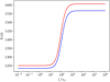Fig. 1 Evolution of the FoM as a function of the inverse of the standard deviation of the new observable, for the test cases considered in Sect. 5.2. In blue, the case where fiducial values of the spectroscopic biases are taken to be equal to the photometric biases (bottom plateau at FoM=1234 and top plateau at FoM=1567). In red, the case with different fiducial values of the spectroscopic biases and photometric biases following the baseline of EP:VII (bottom plateau at FoM=1250 and top plateau at FoM=1606). The FoM includes the information from GCsp, 3×2 pt, and the new observable.

6 Expected improvement on Euclid constraints

6.1 Adjustment of the binning and galaxy selection function in the spectroscopic sample

As seen in the previous section, a substantial improvement in constraints can be achieved, provided the variance on the quantity O is small enough. However, this new observable requires that the selection functions for the two samples are identical (up to a normalisation factor). In order to forecast the potential benefits of this method for the Euclid constraints, it is necessary to adapt the selection function of the spectroscopic galaxy sample to that of the photometric one, in order to ensure that the former is proportional to the latter.

In practice, for each tomographic bin in the photometric sample, it is necessary to select the galaxies in the spectroscopic sample in such a way that the selection function for the two samples is identical. These selected galaxies will then constitute the corresponding population for the spectroscopic sample in the same redshift bin. Throughout this process, we make the assumption that the selection functions retain an identical form, thus ensuring consistency between the two samples. This objective could in principle be achieved by weighting the galaxies in a given sample by the inverse of the selection function, as long as the latter is known. However, the spatially inhomogeneous nature of the resulting Poisson noise could alter the effectiveness of the method. We note that this new selection function for the spectroscopic sample is only considered for the new observable O, as detailed in Sect. 4. When considering GC_sp we still consider narrow redshift bins, to benefit from the radial precision and include all the relevant effects in the modelling. The only difference for GC_sp compared to EP:VII is that we centre the narrow redshift bins on the effective redshifts of the photometric sample. This allows us to have essentially the same galaxy bias for the spectroscopic galaxies in GC_sp and the new observable.

Table 1 presents the numerical values for the galaxy number density in each bin of the spectroscopic sample. The total density of all five bins adds up to 0.35 galaxies per square arcminute, which corresponds to the density of the entire spectroscopic sample. For the photometric probe, we consider the same binning presented in EP:VII, except for a minor change. Since the spec-troscopic survey only goes out to redshift 1.8, we split the last tomographic bin of the photometric sample into two, with half its number density, and therefore consider 11 bins instead of 10. The binning and density values considered for the photometric sample in the redshift range where it overlaps with the spectroscopic sample are presented in Table 2.

6.2 Final results

For each redshift bin where data are available from both surveys, we estimate the total Fisher matrix by adding the contribution from the new observable O to the Fisher matrix computed in the standard case. This allows us to monitor the improvement in various Euclid constraints coming from our new XC2 cross-correlation probe between photometric and spectroscopic surveys, compared to the case where only the correlation between GC_ph and WL is taken into account (i.e., the 3× 2 pt analysis). Figure 2 shows the marginalised constraints for the cosmolog-ical parameters in the optimistic case of the (w₀, w_a) scenario. The addition of the new observable (XC2) clearly improves the constraints and modifies the orientation of correlation ellipses between some parameters, hinting at a breaking of degeneracies. Examination of the triplot of the thirty parameters reveals that the main gain seems to arise on the contours between photometric biases and spectroscopic biases in overlapping redshift bin, although the gain on biases themselves is limited. The appreciable gain on σ₈ likely results from this. A more or less pronounced gain on other parameters follows logically from their correlation with σ₈, see the last line in the triplot of Fig. 2.

Similar comparisons are performed and illustrated in Fig. 3 for the case where the growth index γ is left free. Although no specific behaviour emerges from this comparison, we notice the somewhat logical degeneracy between σ₈ and γ that appears.

Until now, we have followed the EP:VII prescription as much as possible. However, one may wonder whether relaxing these prescriptions could suppress the gain of the addition of the new observable. In order to examine if the hypothesis of scale independent constant bias, we have examine the effect of having more severe scale cut in ℓ for the new observable O. The gains on the FoM are summarised in Table 3 for the semi-pessimistic and optimistic scenarios, with a flat or non-flat cosmology, within general relativity, while for the modified gravity case through the γ model, the comparison of FoMs is presented in Table 4. The percentages correspond to the relative improvement on constraints provided by the XC2 method compared to the baseline analysis. The improvement on the individual cosmological parameters from adding the new observable XC2 is summarized in Fig. 4. This provides a visual comparison of the relative errors on each cosmological parameter and the corresponding FoM for all the cases studied. Although the XC2 method always leads to appreciable improvements, it seems that no regular behaviour can be identified, as some parameters are improved for some cases and not for others. Examination of the triplot of the thirty one parameters reveals that on only some main gain arises on the contours between photometric biases and spectroscopic biases in overlapping redshift bin, but also an appreciable gain on photometric biases, but with almost no gain for spectroscopic biases. The appreciable gain on γ results from this because of tight correlation with photometric biases, and not with spectroscopic biases. Despite the fact that the correlation between γ and σ₈ becomes tighter, no improvement results in σ₈. Again, a more or less pronounced gain on other parameters follows from their correlation with γ, although it remains difficult to identify why the dark energy parameters w₀, w_a are among those to come out on top. In the case of general relativity, the FoM exhibits gains ranging from 18 to 25%. However, when considering cases with γ, substantial gains are observed for both the semi-pessimistic and optimistic scenarios in the flat case. The FoM increases by up to 54% for the semi-pessimistic case and 57% for the optimistic case. In contrast, for the non-flat case with γ, the increase is only 21%. Interestingly, the improvements on the FoM are highest for the flat cosmological case with the modified gravity γ model. We also emphasise that a significant improvement is obtained on γ, by a factor that seems to be roughly the same regardless of the scenario considered. Finally we also compute the improvement when the cut is applied to all the probes: the addition of O: in such a case the relative improvement is the highest. This suggests that the XC2 probe is well-suited to bring interesting constraints for modified gravity models as well as for the GR case.

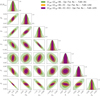Fig. 2 1D normalized likelihood (𝒫/𝒫max) and 2D marginalised Fisher constraints (with 1σ and 2σ limits highlighted) on cosmological parameters for different combinations of probes and in optimistic case/flat space without gravity model considered (no γ growth index parameter). The most stringent constraints are obtained when including the new ratio observable (XC2).

6.3 Taking into account correlations

The results of previous sections were obtained assuming vanishing cross-correlations between O and the C_ℓ. Such terms would appear in the non-diagonal part of the covariance matrix. We have, therefore, evaluated the correlation coefficient κ_ℓ between the two observables o_ℓ (Eq. (24)) and C_ℓ,sp: $${\kappa }_{\ell }=\frac{\langle \left({\widehat{o}}_{\ell }-{\overline{o}}_{\ell }\right)\left(\widehat{C_{\ell ,\text{sp}}}-\overline{C_{\ell ,\text{sp}}}\right)\rangle }{{\sigma }_o{\sigma }_C},$$(35)

in which ${\sigma }_C^2$ stands for the variance of the $\widehat{C_{\ell ,\text{sp}}}$, which is given by $${\sigma }_C=\sqrt{\frac{2}{(2\ell +1)f_{\text{sky}}}}\left(\overline{C_{\ell ,\text{sp}}}+\frac{1}{n_{\text{sp}}}\right).$$(36)

The correlation coefficient κ_ℓ has been estimated accordingly to Eq. (35) and is plotted against ℓ in Fig. 5. Clearly the coefficient κ_ℓ is significant on all scales. The high correlation may undermine the effectiveness of the multi-tracer method as outlined in its simplified version above. On the other hand, employing suitable weighting schemes may help mitigate this degradation (Seljak et al. 2009; Hamaus et al. 2010), but this is beyond the scope of this paper.

6.4 Further strategies for our multi-tracer method

In order to see whether our method could still be useful, we have studied different strategies to get around the difficulty resulting from these strong correlations. In the first strategy, we assume that a fraction α of the survey is devoted to the standard combination of probes in our XC2 synthesis, while the other part 1 − α of the survey is used only for the determination of the observable O. In such a configuration, it is reasonable to assume that the volumes for each observable are independent and therefore O is not correlated to the other probes. The FoM obtained with this strategy is represented by the blue curves in Figs. 6 and 7, where we have considered the optimistic settings. While in the standard scenario (Fig. 6), this strategy does not lead to any improvement in the FoM, one can see from Fig. 7 some gain can be obtained in the modified gravity γ model. In more detail, by devoting 87% of the sky coverage to the standard combination of probes and 13% to the computation of the new observable, the FoM is 9.4 % higher with our multi-tracer approach. This improvement is modest compared to the 58% obtained in Table 4, but it demonstrates that our method can still provide additional information.

In the second strategy, we assume that the 3×2 pt analysis is kept for the full survey, while only a fraction α is used for the GC_sp analysis and (1 − α) for the observable O. This case is represented by the orange curve in Figs. 6 and 7. In the standard model, a modest but non-zero improvement can be seen (4.4%) when 71% of the survey area is used for GC_sp and 29 % is used for the new observable. This improvement is more appreciable in the γ model with a 30% improvement for α = 0.57.

In the final strategy, we assume that the observable O is derived from an independent survey. This assumption necessitates a thorough understanding and mastery of the (photometric) selection functions for the GC_sp and GC_ph surveys. The use of an independent survey then becomes feasible for accessing the observable O. For instance, in the Legacy Survey of Space and Time (LSST) of the Vera C. Rubin Observatory, a significant portion of the observed sky will overlap with the Euclid survey. This, in principle, should enable a precise understanding of the (photometric) selection functions employed in Euclid (GC_sp and GC_ph). Subsequently, the portion of the LSST survey not covered by Euclid can be utilized to estimate the observable O. This case is exemplified by the green curves in Figs. 6 and 7. As one can observe, a significant enhancement is achieved even for α ≃ 0.2–0.3. The improvement is consistently more pronounced in the case of the γ model, suggesting that our multi-tracer approach yields a more substantial benefit in the context of modified gravity theories. However, it is important to note that the expected gain should be evaluated on a case-by-case basis. We note that for this last strategy we consider values of α up to 1.2. This illustrates the improvement on the FoM when using an independent survey with a sky coverage even up to 20% larger than Euclid.

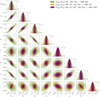Fig. 3 1D normalized likelihood (𝒫/𝒫max) and 2D marginalised Fisher constraints (with 1σ and 2σ limits highlighted) on cosmological parameters for different combinations of probes and in optimistic case/flat space with gravity model considered (γ growth index parameter). The most stringent constraints are also obtained when including the new ratio observable (XC2).

7 Conclusions

Spectroscopic galaxy surveys provide information on both the geometrical distribution of galaxies and their dynamics (through RSDs). Photometric galaxy surveys provide information on both the geometrical distribution of the tracers and the distribution of dark matter through its weak lensing imprint on the shape of galaxies. The information that can be inferred from a survey of a single tracer is primarily limited by the finite volume of the sample, i.e., the sampling noise. In the upcoming generation of wide-field surveys, there will be a significant overlap in the footprint of those two categories of survey. In the case of Euclid, the area overlap between the spectroscopic survey and the photometric survey will be nearly 100%. This overlap offers the opportunity to bring additional information via cross-correlations. Euclid Collaboration: Paganin et al. (in prep.) address the issue of the joint use of the 2D and 3D surveys in Euclid, including their cross-correlations as an additional data vector. Their conclusion is that the covariance between 2D and 3D data can be safely neglected and the addition of the 2D×3D data vector does not significantly change the final constraints. However, when two tracers are available over the same volume, one can also infer the ratio of the bias of the two populations without being limited by the sampling noise (Alimi et al. 1988; Seljak 2009). Given the large number density of objects that will be observed by the upcoming surveys, the Poisson noise limitation is expected to be very small. In this paper, we have introduced a new observable quantity, the ratio of angular (cross-)correlation functions, which provides an additional data vector, enabling a simple implementation of the multi-tracer technique. Using the specifications of Euclid, we have shown that this additional observable provides useful information, resulting in improved estimations of cosmological parameters and, thereby, the FoM of dark energy. Depending on the settings, this improvement can vary from modest (5%) to more substantial (up to 60%). It therefore appears to be a promising approach for enhancing the constraints from future joint analyses when two probes sample the same volume. Interestingly, a gain is achievable even when the biases of the two probes are identical. The details of this gain do not seem to follow a regular pattern. While it leads to a clear improvement in the FoM, constraints on certain cosmological parameters are contingent upon the specific cases studied. For instance, in the general relativity case, no significant enhancement is observed in the constraint on the Hubble parameter, whereas an improvement is observed within the γ model. The constraints on the main targeted parameters, namely the FoM and constraint on γ, consistently exhibit improvement across the various cases investigated. We conclude that the actual benefit of this method needs to be assessed on a case-by-case basis. Finally, we note that the new additional observable we introduced is strongly correlated with the GC_Sp harmonic power spectra. However, we have proposed different strategies, namely splitting the survey into two smaller surveys, or using an independent external survey, to circumvent such a strong correlation. With these strategies we show that the multi-tracer technique proposed in this work can still provide additional valuable information from the combination of probes.

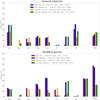Fig. 4 Improvement on cosmological constraints from adding the new observable XC2 compared to the baseline analysis. The top panel shows the improvement for the semi-pessimistic and optimistic settings, and flat and non-flat cosmologies within general relativity. The bottom panel shows the equivalent figure for the modified gravity scenario including the growth index y.

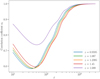Fig. 5 Correlation coefficient κℓ between the two observables oℓ and Qℓ,Sp as a function of ℓ.

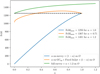Fig. 6 Figure-of-Merit (FoM) as a function of the fraction α of Euclid’s observed sky (fsky). The blue curve represents the combination of a fraction α for the main probes (GCsp and 3×2pt) and (1 – α) for the new observable O. The orange curve represents the combination of a fraction of α for GCsp, together with the full 3×2pt analysis for the full survey and a contribution of (1 – α) for the new observable O. The green curve shows the FoM of the full survey with an additional external contribution from the new observable up to a factor or = 1.2. The dashed line represents the optimal FoM using the standard GCsp and 3×2pt analysis. See the text for additional details on the different cases.

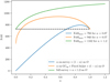Fig. 7 Figure-of-Merit (FoM) as a function of the fraction α of Euclid’s observed sky (fsky). We consider here the modified gravity model with the у parameter. The different curves correspond to the same cases treated in Fig. 6.

Acknowledgements

S. I. thanks the Centre national d’études spatiales (CNES) which supports his postdoctoral research contract. The Euclid Consortium acknowledges the European Space Agency and a number of agencies and institutes that have supported the development of Euclid, in particular the Academy of Finland, the Agenzia Spaziale Italiana, the Belgian Science Policy, the Canadian Euclid Consortium, the French Centre National d’Etudes Spatiales, the Deutsches Zentrum für Luft- und Raumfahrt, the Danish Space Research Institute, the Fundação para a Ciência e a Tecnologia, the Ministerio de Ciencia e Innovación, the National Aeronautics and Space Administration, the National Astronomical Observatory of Japan, the Netherlandse Onder-zoekschool Voor Astronomie, the Norwegian Space Agency, the Romanian Space Agency, the State Secretariat for Education, Research and Innovation (SERI) at the Swiss Space Office (SSO), and the United Kingdom Space Agency. A complete and detailed list is available on the Euclid web site (http://www.euclid-ec.org)..

Appendix A Computation of the variance of the observable ô_ℓ

In this appendix, we provide detailed computations for determining the variance of the observable ô_ℓ . We begin by defining the estimator â_ℓm,sp for the spectroscopic survey as ${\widehat{a}}_{\ell m,\text{sp}}=b_{\text{sp}}{a}_{\ell m}^{\text{DM}}+a_{\ell m,\text{sp}}^p$, where b_sp represents the spectroscopic bias, assumed to be a constant (i.e. no stochasticity in the bias) $a_{\ell m}^{DM}$ denotes the contribution from the matter distribution, and finally $a_{\ell m,\text{sp}}^p$ represents the contribution from the Poisson noise. For simplicity, we initially consider a full sky scenario (f_sky = 1). The Poisson noise is characterized by $\langle a_{\ell m,\text{sp}}^p\rangle =0\text{\hspace{0.17em}and\hspace{0.17em}}\langle {\left|a_{\ell m,\text{sp}}^p\right|}^2\rangle =\frac{1}{n_{\text{sp}}}$. The estimator of the angular power spectrum is given by $${\widehat{C}}_{\ell ,\text{sp}}=\frac{1}{2\ell +1}{\displaystyle \sum _m{\left|{\widehat{a}}_{\ell m,\text{sp}}\right|}^2}=\frac{1}{2\ell +1}{\displaystyle \sum _m\left(b_{\text{sp}}^2{\left|a_{\ell m}^{\text{DM}}\right|}^2+2b_{\text{sp}}\mathrm{Re}\left(a_{\ell m}^{\text{DM}}{a}_{\ell m}^{p*}\right)+{\left|a_{\ell m}^p\right|}^2\right)}.$$(A.1)

The average over Poisson realization yields $$\langle {\widehat{C}}_{\ell ,\text{sp}}\rangle =\frac{1}{2\ell +1}{\displaystyle \sum _m{b}_{\text{sp}}^2}{\left|a_{tm}^{\text{DM}}\right|}^2+\frac{1}{n_{\text{sp}}}={\overline{C}}_{\ell ,\text{sp}}+\frac{1}{n_{\text{sp}}}.$$(A.2)

Here, the quantity ${\overline{C}}_{\ell ,\text{sp}}$ is introduced. For the photometric survey, similar expressions can be formulated, with the Poisson noise being negligible due a significantly larger n_ph compared to n_sp. Consequently, for the photometric angular power spectrum, we have $$\langle {\widehat{C}}_{\ell ,\text{ph}}\rangle \simeq {\overline{C}}_{\ell ,\text{ph}}=\frac{1}{2\ell +1}{\displaystyle \sum _m{b}_{\text{ph}}^2}{\left|a_{\ell m}^{\text{DM}}\right|}^2.$$(A.3)

The observable ô_ℓ can be expressed as $${\widehat{o}}_{\ell }=\frac{{\widehat{C}}_{\ell ,\text{sp}}}{{\widehat{C}}_{\ell ,\text{ph}}}\simeq \frac{{\widehat{C}}_{\ell ,\text{sp}}}{{\overline{C}}_{\ell ,\text{ph}}}={\left(\frac{b_{\text{sp}}}{b_{\text{ph}}}\right)}^2+\frac{1}{(2\ell +1){\overline{C}}_{\ell ,\text{ph}}}{\displaystyle \sum _m\left(2b_{\text{sp}}\mathrm{Re}\left(a_{\ell m}^{\text{DM}}{a}_{\ell m}^{p*}\right)+{\left|a_{\ell m}^p\right|}^2\right)}.$$(A.4)

Hence the mean value of this estimator is given by $$\langle {\widehat{o}}_{\ell }\rangle ={\left(\frac{b_{\text{sp}}}{b_{\text{ph}}}\right)}^2+\frac{1}{n_{\text{sp}}{\overline{C}}_{\ell ,\text{ph}}}.$$(A.5)

The variance is then derived from ${\sigma }_o^2(\ell )=\langle {\left({\widehat{o}}_{\ell }-\langle {\widehat{o}}_{\ell }\rangle \right)}^2\rangle$. Using the property $a_{\ell m}^{*}={(-1)}^m{a}_{\ell ,-m}$ and applying the Isserlis’ theorem to compute $\langle {\left|a_{\ell m}^p\right|}^2{\left|a_{\ell m^{\prime }}^p\right|}^2\rangle$ (assuming Isserlis’ theorem valid for the Poisson noise), straightforward calculations lead to $${\sigma }_o^2(\ell )=\frac{2}{(2\ell +1)f_{\text{sky}}{n}_{\text{sp}}{\overline{C}}_{\ell ,\text{ph}}^2}\left(2{\overline{C}}_{\ell ,\text{sp}}+\frac{1}{n_{\text{sp}}}\right).$$

Here, the f_sky factor has been incorporated, and one recovers expression Eq. (26).

References

All Tables

All Figures

Fig. 1 Evolution of the FoM as a function of the inverse of the standard deviation of the new observable, for the test cases considered in Sect. 5.2. In blue, the case where fiducial values of the spectroscopic biases are taken to be equal to the photometric biases (bottom plateau at FoM=1234 and top plateau at FoM=1567). In red, the case with different fiducial values of the spectroscopic biases and photometric biases following the baseline of EP:VII (bottom plateau at FoM=1250 and top plateau at FoM=1606). The FoM includes the information from GCsp, 3×2 pt, and the new observable.

In the text

	Fig. 2 1D normalized likelihood (𝒫/𝒫max) and 2D marginalised Fisher constraints (with 1σ and 2σ limits highlighted) on cosmological parameters for different combinations of probes and in optimistic case/flat space without gravity model considered (no γ growth index parameter). The most stringent constraints are obtained when including the new ratio observable (XC2).
In the text

	Fig. 3 1D normalized likelihood (𝒫/𝒫max) and 2D marginalised Fisher constraints (with 1σ and 2σ limits highlighted) on cosmological parameters for different combinations of probes and in optimistic case/flat space with gravity model considered (γ growth index parameter). The most stringent constraints are also obtained when including the new ratio observable (XC2).
In the text

	Fig. 4 Improvement on cosmological constraints from adding the new observable XC2 compared to the baseline analysis. The top panel shows the improvement for the semi-pessimistic and optimistic settings, and flat and non-flat cosmologies within general relativity. The bottom panel shows the equivalent figure for the modified gravity scenario including the growth index y.
In the text

	Fig. 5 Correlation coefficient κℓ between the two observables oℓ and Qℓ,Sp as a function of ℓ.
In the text

Fig. 6 Figure-of-Merit (FoM) as a function of the fraction α of Euclid’s observed sky (fsky). The blue curve represents the combination of a fraction α for the main probes (GCsp and 3×2pt) and (1 – α) for the new observable O. The orange curve represents the combination of a fraction of α for GCsp, together with the full 3×2pt analysis for the full survey and a contribution of (1 – α) for the new observable O. The green curve shows the FoM of the full survey with an additional external contribution from the new observable up to a factor or = 1.2. The dashed line represents the optimal FoM using the standard GCsp and 3×2pt analysis. See the text for additional details on the different cases.

In the text

	Fig. 7 Figure-of-Merit (FoM) as a function of the fraction α of Euclid’s observed sky (fsky). We consider here the modified gravity model with the у parameter. The different curves correspond to the same cases treated in Fig. 6.
In the text

References

- Abbott, T. M. C., Aguena, M., Alarcon, A., et al. 2022, Phys. Rev. D, 105, 023520 [CrossRef] [Google Scholar]
- Abramo, L. R., Dinarte Ferri, J. V., Tashiro, I. L., & Loureiro, A. 2022, J. Cosmology Astropart. Phys., 8, 073 [CrossRef] [Google Scholar]
- Albrecht, A., Bernstein, G., Cahn, R., et al. 2006, arXiv e-prints [arXiv:astro-ph/0609591] [Google Scholar]
- Alcock, C., & Paczynski, B. 1979, Nature, 281, 358 [NASA ADS] [CrossRef] [Google Scholar]
- Alimi, J. M., Valls-Gabaud, D., & Blanchard, A. 1988, A&A, 206, L11 [NASA ADS] [Google Scholar]
- Amendola, L., Appleby, S., Avgoustidis, A., et al. 2018, Liv. Rev. Relativ., 21, 2 [NASA ADS] [CrossRef] [Google Scholar]
- Aubourg, É., Bailey, S., Bautista, J. E., et al. 2015, Phys. Rev. D, 92, 123516 [Google Scholar]
- Blanchard, A. 2022, Universe, 8, 479 [NASA ADS] [CrossRef] [Google Scholar]
- Chevallier, M., & Polarski, D. 2001, Int. J. Mod. Phys., D10, 213 [NASA ADS] [CrossRef] [Google Scholar]
- Cropper, M., Pottinger, S., Azzollini, R., et al. 2018, SPIE, 10698, 709 [Google Scholar]
- Eisenstein, D. J., Zehavi, I., Hogg, D. W., et al. 2005, ApJ, 633, 560 [Google Scholar]
- Euclid Collaboration (Blanchard, A., et al.) 2020, A&A, 642, A191 [NASA ADS] [CrossRef] [EDP Sciences] [Google Scholar]
- Euclid Collaboration (Cropper, M., et al.) 2024a, A&A, submitted [arXiv:2405.13492] [Google Scholar]
- Euclid Collaboration (Jahnke, K., et al.) 2024b, A&A, in press, https://doi.org/10.1051/0004-6361/202450786 [Google Scholar]
- Euclid Collaboration (Mellier, Y., et al.) 2024c, A&A, in press, https://doi.org/10.1051/0004-6361/202450010 [Google Scholar]
- Hamaus, N., Seljak, U., Desjacques, V., Smith, R. E., & Baldauf, T. 2010, Phys. Rev. D, 82, 043515 [CrossRef] [Google Scholar]
- Heymans, C., Tröster, T., Asgari, M., et al. 2021, A&A, 646, A140 [NASA ADS] [CrossRef] [EDP Sciences] [Google Scholar]
- Hu, W., & Sawicki, I. 2007, Phys. Rev. D, 76, 104043 [Google Scholar]
- Kilbinger, M. 2015, Rep. Prog. Phys., 78, 086901 [Google Scholar]
- Lahav, O., Lilje, P. ?., Primack, J. R., & Rees, M. J. 1991, MNRAS, 251, 128 [NASA ADS] [CrossRef] [Google Scholar]
- Laureijs, R., Amiaux, J., Arduini, S., et al. 2011, arXiv e-prints [arXiv:1110.3193] [Google Scholar]
- Lesgourgues, J. 2011, arXiv e-prints [arXiv:1104.2932] [Google Scholar]
- Lewis, A., Challinor, A., & Lasenby, A. 2000, ApJ, 538, 473 [Google Scholar]
- Linder, E. V. 2003, Phys. Rev. Lett., 90, 091301 [Google Scholar]
- Linder, E. V. 2005, Phys. Rev. D, 72, 043529 [Google Scholar]
- LoVerde, M., & Afshordi, N. 2008, Phys. Rev. D, 78, 123506 [NASA ADS] [CrossRef] [Google Scholar]
- Ly, A., Marsman, M., Verhagen, J., Grasman, R., & Wagenmakers, E.-J. 2017, arXiv e-prints [arXiv: 1705.01064] [Google Scholar]
- Maciaszek, T., Ealet, A., Gillard, W., et al. 2022, SPIE Conf. Ser., 12180, 121801K [NASA ADS] [Google Scholar]
- McDonald, P., & Seljak, U. 2009, J. Cosmology Astropart. Phys., 10, 007 [CrossRef] [Google Scholar]
- Passaglia, S., Manzotti, A., & Dodelson, S. 2017, Phys. Rev. D, 95, 123508 [CrossRef] [Google Scholar]
- Percival, W. J., & White, M. 2009, MNRAS, 393, 297 [NASA ADS] [CrossRef] [Google Scholar]
- Pozzetti, L., Hirata, C. M., Geach, J. E., et al. 2016, A&A, 590, A3 [NASA ADS] [CrossRef] [EDP Sciences] [Google Scholar]
- Seljak, U. 2009, Phys. Rev. Lett., 102, 021302 [NASA ADS] [CrossRef] [Google Scholar]
- Seljak, U., Hamaus, N., & Desjacques, V. 2009, Phys. Rev. Lett., 103, 091303 [Google Scholar]
- Sugiyama, S., Miyatake, H., More, S., et al. 2023, Phys. Rev. D, 108, 123521 [NASA ADS] [CrossRef] [Google Scholar]
- Tanidis, K., & Camera, S. 2021, MNRAS, 502, 2952 [NASA ADS] [CrossRef] [Google Scholar]
- Tanidis, K., Cardone, V. F., Martinelli, M., et al. 2024, A&A, 683, A17 [NASA ADS] [CrossRef] [EDP Sciences] [Google Scholar]
- Taylor, P. L., & Markovic, K. 2022, Phys. Rev. D, 106, 063536 [NASA ADS] [CrossRef] [Google Scholar]
- Tessore, N. 2017, MNRAS, 471, L57 [NASA ADS] [CrossRef] [Google Scholar]
- Tutusaus, I., Martinelli, M., Cardone, V. F., et al. 2020, A&A, 643, A70 [EDP Sciences] [Google Scholar]
- Wang, Y. 2008, Phys. Rev. D, 77, 123525 [NASA ADS] [CrossRef] [Google Scholar]
- Wang, Y., & Zhao, G.-B. 2020, Res. Astron. Astrophys., 20, 158 [Google Scholar]
- Wang, M. S., Avila, S., Bianchi, D., Crittenden, R., & Percival, W. J. 2020, JCAP 10, 022 [NASA ADS] [CrossRef] [Google Scholar]
- Yahia-Cherif, S., Blanchard, A., Camera, S., et al. 2021, A&A, 649, A52 [NASA ADS] [CrossRef] [EDP Sciences] [Google Scholar]