| Issue |
A&A
Volume 695, March 2025
|
|
|---|---|---|
| Article Number | A280 | |
| Number of page(s) | 24 | |
| Section | Cosmology (including clusters of galaxies) | |
| DOI | https://doi.org/10.1051/0004-6361/202452122 | |
| Published online | 02 April 2025 | |
Euclid preparation
LXV. Determining the weak lensing mass accuracy and precision for galaxy clusters
1
Dipartimento di Fisica e Astronomia “Augusto Righi” – Alma Mater Studiorum Università di Bologna, Via Piero Gobetti 93/2, 40129 Bologna, Italy
2
INAF, Istituto di Radioastronomia, Via Piero Gobetti 101, 40129 Bologna, Italy
3
INAF-Osservatorio di Astrofisica e Scienza dello Spazio di Bologna, Via Piero Gobetti 93/3, 40129 Bologna, Italy
4
INFN-Sezione di Bologna, Viale Berti Pichat 6/2, 40127 Bologna, Italy
5
Université Paris-Saclay, Université Paris Cité, CEA, CNRS, AIM, 91191 Gif-sur-Yvette, France
6
Istituto Nazionale di Fisica Nucleare, Sezione di Bologna, Via Irnerio 46, 40126 Bologna, Italy
7
Université Paris Cité, CNRS, Astroparticule et Cosmologie, 75013 Paris, France
8
Université Côte d’Azur, Observatoire de la Côte d’Azur, CNRS, Laboratoire Lagrange, Bd de l’Observatoire, CS 34229, 06304 Nice Cedex 4, France
9
INAF-Osservatorio Astronomico di Trieste, Via G. B. Tiepolo 11, 34143 Trieste, Italy
10
IFPU, Institute for Fundamental Physics of the Universe, Via Beirut 2, 34151 Trieste, Italy
11
INAF-IASF Milano, Via Alfonso Corti 12, 20133 Milano, Italy
12
Department of Physics “E. Pancini”, University Federico II, Via Cinthia 6, 80126 Napoli, Italy
13
INAF-Osservatorio Astronomico di Capodimonte, Via Moiariello 16, 80131 Napoli, Italy
14
INFN Section of Naples, Via Cinthia 6, 80126 Napoli, Italy
15
Institut für Theoretische Physik, University of Heidelberg, Philosophenweg 16, 69120 Heidelberg, Germany
16
Zentrum für Astronomie, Universität Heidelberg, Philosophenweg 12, 69120 Heidelberg, Germany
17
INAF-Osservatorio Astronomico di Padova, Via dell’Osservatorio 5, 35122 Padova, Italy
18
ESAC/ESA, Camino Bajo del Castillo, s/n., Urb. Villafranca del Castillo, 28692 Villanueva de la Cañada, Madrid, Spain
19
School of Mathematics and Physics, University of Surrey, Guildford, Surrey GU2 7XH, UK
20
INAF-Osservatorio Astronomico di Brera, Via Brera 28, 20122 Milano, Italy
21
INFN, Sezione di Trieste, Via Valerio 2, 34127 Trieste, TS, Italy
22
SISSA, International School for Advanced Studies, Via Bonomea 265, 34136 Trieste, TS, Italy
23
Dipartimento di Fisica e Astronomia, Università di Bologna, Via Gobetti 93/2, 40129 Bologna, Italy
24
Max Planck Institute for Extraterrestrial Physics, Giessenbachstr. 1, 85748 Garching, Germany
25
Universitäts-Sternwarte München, Fakultät für Physik, Ludwig-Maximilians-Universität München, Scheinerstrasse 1, 81679 München, Germany
26
Institut de Physique Théorique, CEA, CNRS, Université Paris-Saclay, 91191 Gif-sur-Yvette Cedex, France
27
Institut d’Astrophysique de Paris, UMR 7095, CNRS, and Sorbonne Université, 98 bis boulevard Arago, 75014 Paris, France
28
INAF-Osservatorio Astrofisico di Torino, Via Osservatorio 20, 10025 Pino Torinese, (TO), Italy
29
Dipartimento di Fisica, Università di Genova, Via Dodecaneso 33, 16146 Genova, Italy
30
INFN-Sezione di Genova, Via Dodecaneso 33, 16146 Genova, Italy
31
Instituto de Astrofísica e Ciências do Espaço, Universidade do Porto, CAUP, Rua das Estrelas, PT4150-762 Porto, Portugal
32
Faculdade de Ciências da Universidade do Porto, Rua do Campo de Alegre, 4150-007 Porto, Portugal
33
Dipartimento di Fisica, Università degli Studi di Torino, Via P. Giuria 1, 10125 Torino, Italy
34
INFN-Sezione di Torino, Via P. Giuria 1, 10125 Torino, Italy
35
Centro de Investigaciones Energéticas, Medioambientales y Tecnológicas (CIEMAT), Avenida Complutense 40, 28040 Madrid, Spain
36
Port d’Informació Científica, Campus UAB, C. Albareda s/n, 08193 Bellaterra, (Barcelona), Spain
37
Institute for Theoretical Particle Physics and Cosmology (TTK), RWTH Aachen University, 52056 Aachen, Germany
38
INAF-Osservatorio Astronomico di Roma, Via Frascati 33, 00078 Monteporzio Catone, Italy
39
Dipartimento di Fisica e Astronomia “Augusto Righi” – Alma Mater Studiorum Università di Bologna Viale Berti Pichat 6/2, 40127 Bologna, Italy
40
Instituto de Astrofísica de Canarias, Calle Vía Láctea s/n, 38204 San Cristóbal de La Laguna, Tenerife, Spain
41
Institute for Astronomy, University of Edinburgh, Royal Observatory, Blackford Hill, Edinburgh EH9 3HJ, UK
42
Jodrell Bank Centre for Astrophysics, Department of Physics and Astronomy, University of Manchester, Oxford Road, Manchester M13 9PL, UK
43
European Space Agency/ESRIN, Largo Galileo Galilei 1, 00044 Frascati, Roma, Italy
44
Université Claude Bernard Lyon 1, CNRS/IN2P3, IP2I Lyon, UMR 5822, Villeurbanne F-69100, France
45
Institute of Physics, Laboratory of Astrophysics, Ecole Polytechnique Fédérale de Lausanne (EPFL), Observatoire de Sauverny, 1290 Versoix, Switzerland
46
Institut de Ciències del Cosmos (ICCUB), Universitat de Barcelona (IEEC-UB), Martí i Franquès 1, 08028 Barcelona, Spain
47
Institució Catalana de Recerca i Estudis Avançats (ICREA), Passeig de Lluís Companys 23, 08010 Barcelona, Spain
48
UCB Lyon 1, CNRS/IN2P3, IUF, IP2I Lyon, 4 rue Enrico Fermi, 69622 Villeurbanne, France
49
Mullard Space Science Laboratory, University College London, Holmbury St Mary, Dorking, Surrey RH5 6NT, UK
50
Departamento de Física, Faculdade de Ciências, Universidade de Lisboa, Edifício C8, Campo Grande, PT1749-016 Lisboa, Portugal
51
Instituto de Astrofísica e Ciências do Espaço, Faculdade de Ciências, Universidade de Lisboa, Campo Grande, 1749-016 Lisboa, Portugal
52
Department of Astronomy, University of Geneva, ch. d’Ecogia 16, 1290 Versoix, Switzerland
53
INFN-Padova, Via Marzolo 8, 35131 Padova, Italy
54
INAF-Istituto di Astrofisica e Planetologia Spaziali, Via del Fosso del Cavaliere, 100, 00100 Roma, Italy
55
Space Science Data Center, Italian Space Agency, Via del Politecnico snc, 00133 Roma, Italy
56
Institut d’Estudis Espacials de Catalunya (IEEC), Edifici RDIT, Campus UPC, 08860 Castelldefels, Barcelona, Spain
57
Institute of Space Sciences (ICE, CSIC), Campus UAB, Carrer de Can Magrans, s/n, 08193 Barcelona, Spain
58
Aix-Marseille Université, CNRS/IN2P3, CPPM, Marseille, France
59
FRACTAL S.L.N.E., calle Tulipán 2, Portal 13 1A, 28231 Las Rozas de Madrid, Spain
60
Dipartimento di Fisica “Aldo Pontremoli”, Università degli Studi di Milano, Via Celoria 16, 20133 Milano, Italy
61
Institute of Theoretical Astrophysics, University of Oslo, P.O. Box 1029 Blindern, 0315 Oslo, Norway
62
Jet Propulsion Laboratory, California Institute of Technology, 4800 Oak Grove Drive, Pasadena, CA 91109, USA
63
Felix Hormuth Engineering, Goethestr. 17, 69181 Leimen, Germany
64
Technical University of Denmark, Elektrovej 327, 2800 Kgs., Lyngby, Denmark
65
Cosmic Dawn Center (DAWN), Copenhagen, Denmark
66
Université Paris-Saclay, CNRS/IN2P3, IJCLab, 91405 Orsay, France
67
Institut de Recherche en Astrophysique et Planétologie (IRAP), Université de Toulouse, CNRS, UPS, CNES, 14 Av. Edouard Belin, 31400 Toulouse, France
68
Max-Planck-Institut für Astronomie, Königstuhl 17, 69117 Heidelberg, Germany
69
NASA Goddard Space Flight Center, Greenbelt, MD 20771, USA
70
Department of Physics and Astronomy, University College London, Gower Street, London WC1E 6BT, UK
71
Department of Physics and Helsinki Institute of Physics, Gustaf Hällströmin katu 2, 00014 University of Helsinki, Finland
72
Université de Genève, Département de Physique Théorique and Centre for Astroparticle Physics, 24 quai Ernest-Ansermet, CH-1211 Genève 4, Switzerland
73
Department of Physics, P.O. Box 64 00014 University of Helsinki, Finland
74
Helsinki Institute of Physics, Gustaf Hällströmin katu 2, University of Helsinki, Helsinki, Finland
75
NOVA Optical Infrared Instrumentation Group at ASTRON, Oude Hoogeveensedijk 4, 7991PD Dwingeloo, The Netherlands
76
Centre de Calcul de l’IN2P3/CNRS, 21 Avenue Pierre de Coubertin, 69627 Villeurbanne Cedex, France
77
University of Applied Sciences and Arts of Northwestern Switzerland, School of Engineering, 5210 Windisch, Switzerland
78
Universität Bonn, Argelander-Institut für Astronomie, Auf dem Hügel 71, 53121 Bonn, Germany
79
INFN-Sezione di Roma, Piazzale Aldo Moro, 2 – c/o Dipartimento di Fisica, Edificio G. Marconi, 00185 Roma, Italy
80
Aix-Marseille Université, CNRS, CNES, LAM, Marseille, France
81
Department of Physics, Institute for Computational Cosmology, Durham University, South Road, Durham DH1 3LE, UK
82
Institut d’Astrophysique de Paris, 98bis Boulevard Arago, 75014 Paris, France
83
European Space Agency/ESTEC, Keplerlaan 1, 2201 AZ Noordwijk, The Netherlands
84
Institut de Física d’Altes Energies (IFAE), The Barcelona Institute of Science and Technology, Campus UAB, 08193 Bellaterra, (Barcelona), Spain
85
DARK, Niels Bohr Institute, University of Copenhagen, Jagtvej 155, 2200 Copenhagen, Denmark
86
Waterloo Centre for Astrophysics, University of Waterloo, Waterloo, Ontario N2L 3G1, Canada
87
Department of Physics and Astronomy, University of Waterloo, Waterloo, Ontario N2L 3G1, Canada
88
Perimeter Institute for Theoretical Physics, Waterloo, Ontario N2L 2Y5, Canada
89
Centre National d’Etudes Spatiales – Centre Spatial de Toulouse, 18 Avenue Edouard Belin, 31401 Toulouse Cedex 9, France
90
Institute of Space Science, Str. Atomistilor, nr. 409 Măgurele, Ilfov 077125, Romania
91
Dipartimento di Fisica e Astronomia “G. Galilei”, Università di Padova, Via Marzolo 8, 35131 Padova, Italy
92
Université St Joseph; Faculty of Sciences, Beirut, Lebanon
93
Departamento de Física, FCFM, Universidad de Chile, Blanco Encalada 2008, Santiago, Chile
94
Satlantis, University Science Park, Sede Bld, 48940 Leioa-Bilbao, Spain
95
Instituto de Astrofísica e Ciências do Espaço, Faculdade de Ciências, Universidade de Lisboa, Tapada da Ajuda, 1349-018 Lisboa, Portugal
96
Universidad Politécnica de Cartagena, Departamento de Electrónica y Tecnología de Computadoras, Plaza del Hospital 1, 30202 Cartagena, Spain
97
INFN-Bologna, Via Irnerio 46, 40126 Bologna, Italy
98
Kapteyn Astronomical Institute, University of Groningen, PO Box 800 9700 AV Groningen, The Netherlands
99
Dipartimento di Fisica, Università degli studi di Genova, and INFN-Sezione di Genova, Via Dodecaneso 33, 16146 Genova, Italy
100
Infrared Processing and Analysis Center, California Institute of Technology, Pasadena, CA 91125, USA
101
Astronomical Observatory of the Autonomous Region of the Aosta Valley (OAVdA), Loc. Lignan 39, I-11020 Nus, (Aosta Valley), Italy
102
ICL, Junia, Université Catholique de Lille, LITL, 59000 Lille, France
103
ICSC – Centro Nazionale di Ricerca in High Performance Computing, Big Data e Quantum Computing, Via Magnanelli 2, Bologna, Italy
104
Instituto de Física Teórica UAM-CSIC, Campus de Cantoblanco, 28049 Madrid, Spain
105
CERCA/ISO, Department of Physics, Case Western Reserve University, 10900 Euclid Avenue, Cleveland, OH 44106, USA
106
Laboratoire Univers et Théorie, Observatoire de Paris, Université PSL, Université Paris Cité, CNRS, 92190 Meudon, France
107
INFN-Sezione di Milano, Via Celoria 16, 20133 Milano, Italy
108
Departamento de Física Fundamental, Universidad de Salamanca, Plaza de la Merced s/n, 37008 Salamanca, Spain
109
Dipartimento di Fisica e Scienze della Terra, Università degli Studi di Ferrara, Via Giuseppe Saragat 1, 44122 Ferrara, Italy
110
Istituto Nazionale di Fisica Nucleare, Sezione di Ferrara, Via Giuseppe Saragat 1, 44122 Ferrara, Italy
111
Université de Strasbourg, CNRS, Observatoire Astronomique de Strasbourg, UMR 7550, 67000 Strasbourg, France
112
Center for Data-Driven Discovery, Kavli IPMU (WPI), UTIAS, The University of Tokyo, Kashiwa, Chiba 277-8583, Japan
113
Ludwig-Maximilians-University, Schellingstrasse 4, 80799 Munich, Germany
114
Max-Planck-Institut für Physik, Boltzmannstr. 8, 85748 Garching, Germany
115
Dipartimento di Fisica – Sezione di Astronomia, Università di Trieste, Via Tiepolo 11, 34131 Trieste, Italy
116
Minnesota Institute for Astrophysics, University of Minnesota, 116 Church St SE, Minneapolis, MN 55455, USA
117
Institute Lorentz, Leiden University, Niels Bohrweg 2, 2333 CA, Leiden, The Netherlands
118
Institute for Astronomy, University of Hawaii, 2680 Woodlawn Drive, Honolulu, HI 96822, USA
119
Department of Physics & Astronomy, University of California Irvine, Irvine, CA 92697, USA
120
Department of Astronomy & Physics and Institute for Computational Astrophysics, Saint Mary’s University, 923 Robie Street, Halifax, Nova Scotia B3H 3C3, Canada
121
Departamento Física Aplicada, Universidad Politécnica de Cartagena, Campus Muralla del Mar, 30202 Cartagena, Murcia, Spain
122
Instituto de Astrofísica de Canarias (IAC); Departamento de Astrofísica, Universidad de La Laguna (ULL), 38200 La Laguna, Tenerife, Spain
123
Université Paris-Saclay, CNRS, Institut d’astrophysique Spatiale, 91405 Orsay, France
124
Department of Physics, Oxford University, Keble Road, Oxford OX1 3RH, UK
125
CEA Saclay, DFR/IRFU, Service d’Astrophysique, Bât. 709, 91191 Gif-sur-Yvette, France
126
Institute of Cosmology and Gravitation, University of Portsmouth, Portsmouth PO1 3FX, UK
127
Department of Computer Science, Aalto University, PO Box 15400 Espoo FI-00 076, Finland
128
Instituto de Astrofísica de Canarias, c/ Via Lactea s/n, La Laguna E-38200, Spain. Departamento de Astrofísica de la Universidad de La Laguna, Avda. Francisco Sanchez, La Laguna E-38200, Spain
129
Ruhr University Bochum, Faculty of Physics and Astronomy, Astronomical Institute (AIRUB), German Centre for Cosmological Lensing (GCCL), 44780 Bochum, Germany
130
Univ. Grenoble Alpes, CNRS, Grenoble INP, LPSC-IN2P3, 53, Avenue des Martyrs, 38000 Grenoble, France
131
Department of Physics and Astronomy, Vesilinnantie 5, 20014 University of Turku, Finland
132
Serco for European Space Agency (ESA), Camino bajo del Castillo, s/n, Urbanizacion Villafranca del Castillo, Villanueva de la Cañada, 28692 Madrid, Spain
133
ARC Centre of Excellence for Dark Matter Particle Physics, Melbourne, Australia
134
Centre for Astrophysics & Supercomputing, Swinburne University of Technology, Hawthorn, Victoria 3122, Australia
135
School of Physics and Astronomy, Queen Mary University of London, Mile End Road, London E1 4NS, UK
136
Department of Physics and Astronomy, University of the Western Cape, Bellville, Cape Town 7535, South Africa
137
ICTP South American Institute for Fundamental Research, Instituto de Física Teórica, Universidade Estadual Paulista, São Paulo, Brazil
138
IRFU, CEA, Université Paris-Saclay, 91191 Gif-sur-Yvette Cedex, France
139
Oskar Klein Centre for Cosmoparticle Physics, Department of Physics, Stockholm University, Stockholm SE-106 91, Sweden
140
Astrophysics Group, Blackett Laboratory, Imperial College London, London SW7 2AZ, UK
141
INAF-Osservatorio Astrofisico di Arcetri, Largo E. Fermi 5, 50125 Firenze, Italy
142
Dipartimento di Fisica, Sapienza Università di Roma, Piazzale Aldo Moro 2, 00185 Roma, Italy
143
Aurora Technology for European Space Agency (ESA), Camino bajo del Castillo, s/n, Urbanizacion Villafranca del Castillo, Villanueva de la Cañada, 28692 Madrid, Spain
144
Centro de Astrofísica da Universidade do Porto, Rua das Estrelas, 4150-762 Porto, Portugal
145
HE Space for European Space Agency (ESA), Camino bajo del Castillo, s/n, Urbanizacion Villafranca del Castillo, Villanueva de la Cañada, 28692 Madrid, Spain
146
Institute of Astronomy, University of Cambridge, Madingley Road, Cambridge CB3 0HA, UK
147
Department of Astrophysics, University of Zurich, Winterthurerstrasse 190, 8057 Zurich, Switzerland
148
INAF-Osservatorio Astronomico di Brera, Via Brera 28, 20122 Milano, Italy, and INFN-Sezione di Genova, Via Dodecaneso 33, 16146 Genova, Italy
149
Theoretical Astrophysics, Department of Physics and Astronomy, Uppsala University, Box 515 751 20 Uppsala, Sweden
150
Department of Physics, Royal Holloway, University of London, TW20 0EX London, UK
151
Department of Physics and Astronomy, University of California, Davis, CA 95616, USA
152
Department of Astrophysical Science, Peyton Hall, Princeton University, Princeton, NJ 08544, USA
153
Cosmic Dawn Center (DAWN), Copenhagen, Denmark
154
Niels Bohr Institute, University of Copenhagen, Jagtvej 128, 2200 Copenhagen, Denmark
155
Center for Cosmology and Particle Physics, Department of Physics, New York University, New York, NY 10003, USA
156
Center for Computational Astrophysics, Flatiron Institute, 162 5th Avenue, 10010 New York, NY, USA
⋆ Corresponding author; lorenzo.ingoglia@inaf.it
Received:
5
September
2024
Accepted:
16
December
2024
The ability to measure unbiased weak-lensing (WL) masses is a key ingredient to exploit galaxy clusters as a competitive cosmological probe with the ESA Euclid survey or future missions. We investigate the level of accuracy and precision of cluster masses measured with the Euclid data processing pipeline. We use the DEMNUni-Cov N-body simulations to assess how well the WL mass probes the true halo mass, and, then, how well WL masses can be recovered in the presence of measurement uncertainties. We consider different halo mass density models, priors, and mass point estimates, that is the biweight, mean, and median of the marginalised posterior distribution and the maximum likelihood parameter. WL mass differs from true mass due to, for example, the intrinsic ellipticity of sources, correlated or uncorrelated matter and large-scale structure, halo triaxiality and orientation, and merging or irregular morphology. In an ideal scenario without observational or measurement errors, the maximum likelihood estimator is the most accurate, with WL masses biased low by ⟨bM⟩= − 14.6 ± 1.7% on average over the full range M200c > 5 × 10¹³ M⊙ and z < 1. Due to the stabilising effect of the prior, the biweight, mean, and median estimates are more precise, that is with smaller intrinsic scatter. The scatter decreases with increasing mass and informative priors can significantly reduce the scatter. Halo mass density profiles with a truncation provide better fits to the lensing signal, while the accuracy and precision are not significantly affected. We further investigate the impact of various additional sources of systematic uncertainty on the WL mass estimates, namely the impact of photometric redshift uncertainties and source selection, the expected performance of Euclid cluster detection algorithms, and the presence of masks. Taken in isolation, we find that the largest effect is induced by non-conservative source selection with ⟨bM⟩= − 33.4 ± 1.6%. This effect can be mostly removed with a robust selection. As a final Euclid-like test, we combine systematic effects in a realistic observational setting and find ⟨bM⟩= − 15.5 ± 2.4% under a robust selection. This is very similar to the ideal case, though with a slightly larger scatter mostly due to cluster redshift uncertainty and miscentering.
Key words: gravitational lensing: weak / galaxies: clusters: general / dark matter
© The Authors 2025
 Open Access article, published by EDP Sciences, under the terms of the Creative Commons Attribution License (https://creativecommons.org/licenses/by/4.0), which permits unrestricted use, distribution, and reproduction in any medium, provided the original work is properly cited.
This article is published in open access under the Subscribe to Open model. Subscribe to A&A to support open access publication.
1. Introduction
Galaxy clusters are robust tracers of the matter density field (e.g. Allen et al. 2011). They are hosted in dark matter haloes, which are seeded by initial perturbations of the matter overdensity field and subsequently form via the hierarchical growth of structure. At the present time, many clusters have reached virial equilibrium and are among the most massive gravitationally bound systems in the Universe Voit 2005; Borgani 2008.
Clusters probe the distribution and evolution of cosmic structures through their abundance, spatial distribution, and as a function of their redshift and mass. The high-mass end of the halo-mass function has been measured by cluster surveys and is particularly sensitive to dark energy Vikhlinin et al. 2009; Mantz et al. 2015; Planck Collaboration XXII 2016; Costanzi et al. 2019; Bocquet et al. 2019. Surveys measure baryonic mass proxies, such as richness, the Sunyaev–Zeldovich effect, and X-ray luminosity, from intracluster gas or the distribution of galaxies. A mass-observable relation is additionally needed to anchor these survey measurements to the halo mass function. Therefore, unbiased cluster mass measurements are essential to accurately constrain cosmological parameters Giocoli et al. 2021; Ingoglia et al. 2022.
One reliable method to measure galaxy cluster masses is via weak gravitational lensing (henceforth WL, for a review see Bartelmann & Schneider 2001; Schneider 2006; Kilbinger 2015), an effect by which the images of background galaxies are distorted due to a foreground mass. The inference of cluster masses from WL is close to unbiased Becker & Kravtsov 2011; Oguri & Hamana 2011; Bahé et al. 2012, independent of the dynamical state of the cluster, and probes the entire halo mass, which is dominated by dark matter Hoekstra et al. 2012, 2015; Umetsu et al. 2014, 2016; Sereno et al. 2018. Individual WL cluster masses have successfully been used in cluster count measurements to constrain cosmology Bocquet et al. 2019; Costanzi et al. 2021.
In the past decade, the emergence of large and deep photometric surveys, such as the Canada-France-Hawaii Telescope Legacy Survey (CFHTLS; Heymans et al. 2012), the Kilo-Degree Survey (KiDS; de Jong et al. 2013), the Hyper Suprime-Cam Subaru Strategic Program (HSC-SSP; Aihara et al. 2018; Miyazaki et al. 2018), and the Dark Energy Survey (DES; Abbott et al. 2018), has enabled precise WL mass measurements of large samples of individual galaxy clusters (e.g. Sereno et al. 2017, 2018; Umetsu et al. 2020; Murray et al. 2022; Euclid Collaboration: Sereno et al. 2024). These measurements have laid the groundwork for the next generation of surveys.
The ESA Euclid Survey (Laureijs et al. 2011; Euclid Collaboration: Scaramella et al. 2022; Euclid Collaboration: Mellier et al. 2024) will observe galaxies over a significant fraction of the sky (the nominal area of the wide survey is 14000 deg2) in wide optical and near-infrared bands. From the photometric galaxy catalogue, galaxy clusters will be identified using two detection algorithms, AMICO Bellagamba et al. 2011, 2018; Euclid Collaboration: Adam et al. 2019 and PZWav Gonzalez 2014; Euclid Collaboration: Adam et al. 2019; Thongkham et al. 2024, and their masses will be estimated with the Euclid combined clusters and WL pipeline COMB-CL1 using the shape catalogue constructed from the high-resolution images taken with the VIS instrument Cropper et al. 2012; Euclid Collaboration: Cropper et al. 2024. While a comprehensive description of the code structure and methods employed by COMB-CL will be presented in a forthcoming paper (Euclid Collaboration: Farrens et al., in prep.), a brief overview of the pipeline can be found in Euclid Collaboration: Sereno et al. 2024.
Measuring individual galaxy cluster masses using the WL signal is challenging due to large intrinsic scatter in the shapes of galaxies (shape noise), contamination from foreground or cluster member galaxies in the source catalogue, and uncertainty in the photometric redshifts (henceforth photo-z) of source galaxies McClintock et al. 2019; Euclid Collaboration: Lesci et al. 2024. Other issues, such as miscentring Sommer et al. 2022, triaxiality Becker & Kravtsov 2011, or merging Lee et al. 2023, can also create a bias with respect to the true cluster mass. Numerical simulations are powerful tools to measure these various effects as they provide a true halo mass and allow us to test how individual systematic effects influence the lensing signal. Recent works on hydrodynamical simulations have made significant progress in determining bias and uncertainties in WL mass calibration Grandis et al. 2019, 2021.
Euclid Collaboration: Giocoli et al. (2024, referred hereafter as ECG) perform a systematic study of the cluster mass bias based on the Three Hundred Project Cui et al. 2018, 2022 simulations, a sample of 324 high-massive clusters resimulated with hydrodynamical physics. They examine the impact of cluster projection effects, different halo profile modelling, and free, fixed, or mass-dependent concentration on the measured WL mass in the Euclid Wide Survey.
In this paper, we present an analysis, complementary to ECG, of the bias affecting the WL cluster mass estimates obtained with COMB-CL in a Euclid-like setting. Using a large N-body simulation data set, we measure the mass bias for different statistical point estimates over the broad mass range M200c > 5 × 10¹³ M⊙, where M200c is the mass enclosed by a spherical overdensity 200 times the critical density of the Universe at the cluster redshift. Our analysis differs from the Three Hundred study in several ways. Firstly, the distribution in mass and redshift of the simulations we use is more representative of the clusters that Euclid is expected to detect. Secondly, while the Three Hundred study focuses on the most massive clusters, we here perform a WL mass bias analysis on a larger sample of clusters that includes relatively low-mass clusters. Furthermore, we study the impact of individual and combined systematic effects on both lens and source catalogues. In addition to shape noise, we assess the impact of uncertain source redshift estimates, different algorithms used for cluster detection in Euclid (AMICO or PZWav), cluster miscentring, masks, models of the halo density profile, and priors.
In this work, we assume a spatially flat ΛCDM model consistent with the simulation data adopted. All references to ‘ln’ and ‘log’ stand for the natural and decimal logarithms, respectively. Masses expressed in logarithms are log(M/M⊙) or ln(M/M⊙).
This paper is part of a series presenting and discussing WL mass measurements of clusters exploiting the COMB-CL pipeline. Euclid Collaboration: Farrens et al., (in prep.) describes the algorithms and code, Euclid Collaboration: Sereno et al. 2024 tests the robustness of COMB-CL through the reanalysis of precursor photometric surveys, and Euclid Collaboration: Lesci et al. 2024 introduces a novel method for colour selection of background galaxies.
The present paper discusses the simulation data used for the analysis (Sect. 2), methods for lensing mass measurements (Sect. 3), accuracy and precision of WL mass estimates (Sect. 4), impacts of various systematic effects on the mass bias (Sect. 5), and the role of halo profile modelling and priors (Sect. 6). All systematic effects are considered together in Sect. 7, and a conclusive summary and discussion are presented in Sects. 8; and 9, respectively.
2. Simulated data
In this work, we are interested in simulated data of massive dark matter haloes, typical of those that host galaxy clusters. The following section presents the simulations used in the paper for a consistent test of individual cluster WL mass measurements.
2.1. DEMNUni-Cov
The Dark Energy and Massive Neutrino Universe (DEMNUni, Carbone et al. 2016; Parimbelli et al. 2022) is a set of cosmological N-body simulations that follows the redshift evolution of the large-scale structure (LSS) of the Universe with and without massive neutrinos. These simulations are designed to study covariance matrices of various cosmological observables, such as galaxy clustering, WL, and complementary CMB data. Their large volume and high resolution make them ideal for cluster WL studies.
In this work, we use one of the DEMNUni-Cov independent N-body simulations Parimbelli et al. 2021; Baratta et al. 2023. It consists of the gravitational evolution of 10243 CDM (Cold Dark Matter) particles with mass resolution mp ∼ 8 × 10¹⁰ h−1 M⊙ in a box of comoving size equal to 1 h−1 Gpc on a side. Initial conditions are generated at z = 99, using a theoretical linear power spectrum calculated using CAMB Lewis et al. 2000. The considered cosmological parameters are consistent with Planck Collaboration VI 2020; specifically, Ωcdm = 0.27, Ωb = 0.05, Hubble constant H0 = 67 km s−1 Mpc−1, initial scalar amplitude As = 2.1265 × 10⁻⁹, and primordial spectra index ns = 0.96. 63 snapshots are stored while running the simulations from redshift z = 99 to z = 0. This is sufficient to construct continuous past-light cones up to high redshifts.
Lensing past-light cone simulations are constructed with the MapSim pipeline routines Giocoli et al. 2015. The size of the simulation box is sufficient to design a pyramidal past-light cone with a square base up to z = 4 and an aperture of 10 degrees on a side. A total of 43 lens planes are constructed by reading 40 stored snapshots from z = 0 to z = 4, replicating the boxes five times along the light-cone, and stacking the boxes Tessore et al. 2015; Giocoli et al. 2017, 2018a,b; Castro et al. 2018; Peel et al. 2018; Hilbert et al. 2020; Boyle et al. 2021. Rays are shot through these lens planes in the Born approximation regime from various source redshifts, located at the upper bound of each lens plane, down to the observer placed at the vertex of the pyramid. The convergence and shear maps are computed with the MOKA library pipeline Giocoli et al. 2012 and resolved with 4096 pixels, which correspond to a pixel resolution of  , adequate for WL cluster studies.
The Born approximation is reasonable given the resolution and the volume of DEMNUni-Cov. It is worth underlining that this assumption is an excellent approximation on small angular scales in the WL regime and remains valid in the cluster lensing regime, as long as we avoid the core region of the cluster Schäfer et al. 2012. This method has been used and tested on a variety of cosmological simulations Tessore et al. 2015; Castro et al. 2018; Giocoli et al. 2018b; Euclid Collaboration: Ajani et al. 2023 and recently compared with other algorithms Hilbert et al. 2020. From the calibration of shear measured in Euclid-like surveys, we expect a sub-percent level of accuracy Cropper et al. 2013. We extract the corresponding shear catalogue, as done in Euclid Collaboration: Ajani et al. 2023, by populating the past-light cone with the expected Euclid source redshift distribution for the wide survey Euclid Collaboration: Blanchard et al. 2020.
2.2. Source and lens specifics
2.2.1. Sources
An unbiased shear catalogue of unclustered sources is derived from the DEMNUni-Cov past-light cones with information about source position (RA, Dec), redshift, shear components γ1, γ2, and convergence κ. The sources are uniformly spatially distributed with a number density of 30 arcmin−2 up to z = 3.
We simulate observed ellipticities, including both intrinsic ellipticity and shear distortion, based on the simulated shear and convergence. In the WL regime, where γ ≪ 1 and κ ≪ 1, the average intrinsic shape of randomly oriented sources has zero ellipticity, and the ensemble average observed ellipticity of the sources is equivalent to the reduced shear g ≡ γ/(1 − κ).
Due to the weak deformation of the source shape, the shear components are dominated by shot noise. We simulate observed ellipticities by adding shape noise to the reduced shear as Seitz & Schneider 1997
where the intrinsic ellipticity of the source ϵs is normally generated assuming a shape dispersion of σϵ = 0.26, as expected for Euclid Euclid Collaboration: Martinet et al. 2019; Euclid Collaboration: Ajani et al. 2023.
For our analysis, we consider either true simulated source redshifts, or redshifts scattered to mimic the process of a photometric redshift measurement, see Sect. 5.1. We discuss two sets of simulated photo-zs with appropriate selections: one accounting for outliers and using a non-conservative cut, and another with more reliable photo-zs and a robust cut. We do not consider uncertainties in the source position, which are negligible in the WL regime. The astrometric uncertainty for Euclid sources is lower than 15″ Euclid Collaboration: Moneti et al. 2022, and the effect on the signal is negligible in WL analyses.
2.2.2. Lenses
The lens halo catalogue extracted from the DM haloes provides the following information: position (RA, Dec); redshift of the deflector zd < 1; mass M200c > 5 × 10¹³ M⊙. The DEMNUni-Cov sample consists of 6155 clusters. Cuts on the halo catalogue are made at low mass, M200c > 5 × 10¹³ M⊙, and high redshift, zd < 1, to focus on the broad mass-redshift region of Euclid-detected clusters for which the WL mass can be obtained with a large signal-to-noise ratio Euclid Collaboration: Adam et al. 2019; Euclid Collaboration: Sereno et al. 2024.
Figure 1 depicts the distribution of selected clusters. The mass distribution peaks at the lower bound of the sample, while the cluster redshifts are more uniformly distributed above zd > 0.4.
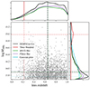 |
Fig. 1. Distribution of the DEMNUni-Cov clusters and of the Three Hundred clusters (ECG) in the mass-redshift plane. The marginalised distribution of the redshift and mass of the clusters is shown in the top and right panels, respectively. Distributions are normalised to the full DEMNUni-Cov sample. Distributions of AMICO and PZWav-like selected objects (see Sect. 5.2) are also shown. The median is shown with dashed lines. The mean of the Gaussian prior on mass (see Sect. 6.2) is shown on the right panel as a dotted line. |
For our analysis, we consider either the full sample with true simulated lens position and redshift or subsamples with scattered values to mimic the detection process, see Sect. 5.2. Two Euclid-like cluster catalogues are generated, simulating the centre positions and cluster distributions using the selection functions of the detection algorithms AMICO Bellagamba et al. 2011, 2018; Euclid Collaboration: Adam et al. 2019 and PZWav Gonzalez 2014; Euclid Collaboration: Adam et al. 2019; Thongkham et al. 2024.
2.3. Three Hundred
We compare our findings with the recent results presented by ECG and based on the Three Hundred simulations. These runs consist of 324 hydrodynamical simulated regions by the Three Hundred Collaboration Cui et al. 2018, 2022 centred on the most massive clusters (M200c ≳ 8 × 10¹⁴ h−1 M⊙) identified at zd = 0 in a box size of 1 Gpc on a side, where haloes have been identified using AHF (Amiga’s Halo Finder, Knollmann & Knebe 2009).
The WL mass measurements from the Three Hundred simulations are discussed in Sect. 4.3. In ECG, the analyses of cluster WL mass bias are performed using the projections of lensing signals along different orientations of the mass tensor ellipsoid. The authors consider the haloes at zd = 0.22 and three random projections, raising the effective number of cluster mass measurements to 972. The authors fit a Baltz–Marshall–Oguri model Baltz et al. 2009, as implemented in the CosmoBolognaLib2 Marulli et al. 2016 libraries, with fixed, free, or mass-constrained values of the concentration parameter and various values of the truncated radius, finding that the results are sensitive to the model parameter choices.
The mass and redshift range of DEMNUni-Cov clusters more closely resemble what is expected from Euclid observations than the mass range of the Three Hundred Project. In particular, the DEMNUni-Cov catalogue focuses on a lower cluster mass range; thus, the cluster sample is much larger than that of the Three Hundred.
For the Three Hundred simulations, the WL signal is derived by projecting the particles in a slice of depth ± 5 Mpc in front and behind the cluster onto a single lens plane to focus on the lensing effect of the main halo. On the contrary, a full multiplane ray-tracing is performed in DEMNUni-Cov simulations, and we can account for the full projected mass density distribution from the source redshift to the observer located at z = 0, including the effects of LSS and correlated matter around the main halo.
The large DEMNUni-Cov sample allows us to measure WL mass bias with systematics similar to those we expect from Euclid data in the low-mass range. We also look at the precision of the lensing signal in different redshift bins as DEMNUni-Cov haloes are distributed up to redshift z = 1. It is worth highlighting that hydrodynamical effects primarily impact the lensing signal in the cluster core, R ≲ 100 kpc (e.g. Springel et al. 2008). In order to avoid the impact of these effects, we only model the WL mass outside of this region.
3. Lensing measurements
In this section, we detail the methodology we use to estimate WL cluster masses from the data presented in Sect. 2. In particular, we describe how we measure the WL signal in radial bins and fit the data to a fiducial model.
3.1. Shear profiles
3.1.1. Lensing properties
The intrinsic shapes of galaxies are distorted by the matter inhomogeneities along the line of sight, which include galaxy clusters. This yields isotropic and anisotropic deformations of the intrinsic ellipticity of the galaxies: the convergence κ and the shear γ, respectively. The lensing information of an intervening axially symmetric lens on a single source plane is encoded by the convergence Bartelmann & Schneider 2001; Schneider 2006; Kilbinger 2015

and by excess surface density, which can be expressed in terms of the tangential component of the shear,

Here, the surface mass density Σ is the projected matter density, and the excess surface mass density ΔΣ is the difference between the mean value of the surface mass density calculated over a disc with a radius that comprises the projected distance between the lens centre and the source, and its local value. The critical surface mass density Σcr is defined as
where c is the speed of light in vacuum, G is the gravitational constant, and Ds, Dd and Dds are the angular diameter distances from the observer to the source, from the observer to the lens, and from the lens to the source, respectively.
We also introduce the observed quantity ΔΣgt analogous to Eq. (3),

In the following, we will use the excess surface mass density as in Eq. (5).
3.1.2. Profile measurement
Because the intrinsic shape noise dominates the lensing signal of individual sources, we derive density profiles by measuring the mean source shear in fixed radial bins. The averaged lensing observable is calculated over the j-th radial annulus as
where the weight of the i-th source is  . We consider a uniform lensing weight related to shape estimate uncertainties, ws = 1/σϵ2. In this study, the statistical uncertainty of the lensing estimate accounts for the shape noise of the background sources, and it is computed as the uncertainty of the weighted mean,
Here, we do not account for bias in ellipticity measurements and shear calibration in the lensing signal, unlike methods applied to real survey data (e.g. McClintock et al. 2019).
We select background sources with the following criterion for the source photo-z

where Δz is a secure interval that minimises the contamination. We set Δz = 0.1 to be twice the threshold value defined in Medezinski et al. 2018.
Shears are measured at the shear-weighted radial position Sereno et al. 2017
The effective radius is computed with α = 1.
To calculate Σcr in a radial bin with N background sources, we derive the effective surface critical density as Sereno et al. 2017
In addition, we define the WL signal-to-noise ratio per halo as Sereno et al. 2017
Here, ⟨ΔΣgt⟩ is the average lensing observable measured in the full radial range of the lens, while the error budget δt accounts for the contribution of statistical uncertainties and cosmic noise, see Sect. 3.2.2.
In the following, we consider shears averaged in eight logarithmically equispaced radial bins covering the range [0.4, 4.0] Mpc from the cluster centre, similar to the binning scheme set in Euclid Collaboration: Sereno et al. 2024.
3.2. Mass inference
3.2.1. Density models
We derive WL masses by constraining a fiducial model of the halo density profile with the measured shear density profiles. Modelling the mass density distribution of the haloes is challenging as it results from various physical effects, for example, miscentering Yang et al. 2006; Johnston et al. 2007 or the contribution of correlated matter Covone et al. 2014; Ingoglia et al. 2022. In this study, as a reference model, we assume the simple but effective Navarro–Frenk–White (NFW) density profile Navarro et al. 1996, 1997
where ρs is the scale density, and rs the scale radius.
We also consider a truncated version of the NFW profile 2009JCAP...01..015B, known as the Baltz–Marshall–Oguri (BMO) profile,
where rt is the truncation radius set to rt = 3r200c Oguri & Hamana 2011; Bellagamba et al. 2019.
The mass density and the excess surface mass density can be expressed as a function of mass, M200c, and concentration c200c. For the fitting parameters, we consider the logarithm (base 10) of mass and concentration.
3.2.2. Fitting procedure
Following a Bayesian approach, we derive the posterior probability density function p of parameters p = [log M200c, log c200c] given the likelihood function ℒ and the prior pprior as

where ⟨ΔΣgt⟩ are the data, ℒ ∝ exp(−χ2/2), and
![$$ \begin{aligned} \chi ^2 = \sum \limits _{i, j} \!\left[ \langle \Delta \Sigma _{g_{\rm t}} \rangle _i - \Delta \Sigma _{g_{\rm t}} (\langle R \rangle _i, \boldsymbol{\mathrm{p}}) \right]^{-1} \!{\mathsf{C }}_{ij}^{-1}\! \left[ \langle \Delta \Sigma _{g_{\rm t}} \rangle _j - \Delta \Sigma _{g_{\rm t}} (\langle R \rangle _j, \boldsymbol{\mathrm{p}}) \right], \end{aligned} $$](/articles/aa/full_html/2025/03/aa52122-24/aa52122-24-eq17.gif)
where the sum runs over the radial bins i, j. We measure the reduced χ2 as

where Nd.o.f is the number of degrees of freedom.
In the present analysis, the covariance matrix C accounts for shape noise, δΔΣgt, and cosmic noise, ΔΣLSS, as Gruen et al. 2015; Sereno et al. 2018
In the above equation, Cstat is a diagonal matrix with terms  , and C
 characterises the effects of uncorrelated LSS in each pair of annular bins (Δθi, Δθj) Schneider et al. 1998; Hoekstra 2003

where Pk(l) is the effective projected lensing power spectrum and the function g is the filter.
We adopt a uniform prior with ranges log M200c ∈ [13, 16] and log c200c ∈ [0, 1]. In Sect. 6.2, we show the impact of using a Gaussian prior on the mass inference.
We sample the posterior distribution using an affine invariant Markov Chain Monte Carlo (MCMC) approach Foreman-Mackey et al. 2013. Each Markov chain runs for 3200 steps starting from initial values randomly taken from a bivariate normal distribution of mean mass log M200c = 14 and mean concentration log c200c = 0.6. The posterior is estimated after removing a burn-in phase, which is assumed to be four times the autocorrelation time of the chain.
3.2.3. Mass point estimators
The MCMC chains sample the posterior distribution of the model parameters, and can be summarised with a point estimate of the WL mass. Cluster masses measured using individual shear density profiles may vary depending on the statistical estimator employed. In the following sections, we compare WL masses recovered using several different point estimators. We look at the mean, and the related standard deviation, or the median of the marginalised posterior mass distribution, for which the associated uncertainties are the standard deviation, and the 16th and 84th percentiles of the sample distribution. We also consider the biweight location and scale, hereafter referred to as CBI and SBI, respectively, which are robust statistics for summarising a distribution Beers et al. 1990. Finally, we look at the maximum likelihood max(ℒ), hereafter referred to as ML.
3.3. Cluster ensemble average
By averaging the shear signal across an ensemble of clusters, the precision of lensing profile measurements improves in comparison to those obtained from a single lens. Therefore, the uncertainties on the lensing mass measurements are also reduced. This provides a complementary method to single lens mass bias analyses for quantifying the impact of systematic effects.
We measure the surface mass density in the j-th radial annulus similarly to Eq. (20) with the average quantity
where ⟨ΔΣgt⟩j, n is the surface mass density in the j-th radial bin, see Eq. (6), of the n-th cluster, and the weight can be expressed in terms of the uncertainty on the weighted mean, see Eq. (7), as WΔΣ, j, n = δΔΣgt, j, n−2.
The associated uncertainty on the averaged cluster lensing profile accounts for the total shape noise of the sources. For this analysis, contributions from correlated or uncorrelated large-scale structure are not considered in the covariance of the averaged lensing profiles. In the following, any observable O measured by fitting the averaged lensing profile, for instance, mass or concentration, is quoted as O⟨ΔΣ⟩.
Figure 2 displays the average shear profiles for the samples and cases discussed in Sects. 4, and 5, and the density model for the ML point estimate. Mass and concentration are estimated at the mean lens redshift of the cluster sample considered, as measured in Eq. (20), and given in Table 1 along with the corresponding reduced χ2.
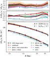 |
Fig. 2. Average excess surface density and maximum likelihood NFW / BMO density fitted models. The figure shows the density profiles for the LSS plus shape noise (Sect. 4), non-conservative photo-z selection (Sect. 5.1.1), robust photo-z selection (Sect. 5.1.2), AMICO-like sample (Sect. 5.2), PZWav-like sample (Sect. 5.2), masks (Sect. 5.3), BMO model (Sect. 6.1), and combined effects (Sect. 7). Signals are shown either for the full sample, or for the massive subsample at log Msim ≥ 14.7. The top panels show the relative change with respect to the fiducial shape and LSS noise shear data (points), and with respect to their models (lines). |
ML logarithmic mass and concentration of the NFW fit to average cluster lensing profiles, and associated reduced χ2.
For a given population of N galaxy clusters, we compute the ensemble average of the observable O, such as the mass bias or the mass change, see Eqs. (23), (25), as a lensing-weighted mean (e.g. Umetsu et al. 2014)
where On is the observable measured for the n-th cluster, and WΔΣ, n = ∑jWΔΣ, j, n is the total weight of the n-th cluster, see Eq. (7). The associated scale of the weighted mean in Eq. (20) is calculated as
4. Accuracy and precision for WL masses for intrinsic scatter and noise
Simulated data can be used to probe the accuracy and precision of WL cluster mass measurements, as the true halo masses are known a priori. In this section, we assess the WL mass estimates we obtained for DEMNUni-Cov clusters measured from unbiased catalogues. By unbiased catalogues, we mean that the catalogues are not affected by measurement errors, and the WL mass differs from the true mass only for intrinsic noise and bias. This can be due to a number of effects. For example, due to intrinsic ellipticity, the measured shape of a source may differ from the underlying reduced shear. LSS distorts the source shape. Mass derived assuming the spherical approximation may be scattered due to traxiality and cluster orientation, or irregular morphology Meneghetti et al. 2010, 2014; Becker & Kravtsov 2011; Giocoli et al. 2014; Herbonnet et al. 2022; Euclid Collaboration: Giocoli et al. 2024. These effects are all accounted for in simulated N-body samples. We refer to this case as ‘LSS + shape noise’.
4.1. Precision of the lensing signal
To assess the precision to which the WL signal can be measured, we first calculate (S/N)WL for each lens as in Eq. (11). In Fig. 3, we plot the distribution of (S/N)WL for clusters binned in mass and redshift. For each bin, we show the CBI value. We find the highest (S/N)WL values for the few high-mass and low-redshift haloes, while the more numerous distant or low-mass objects have lensing signals largely dominated by noise.
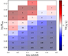 |
Fig. 3. (S/N)WL of DEMNUni-Cov clusters in bins of mass and redshift, computed as the CBI of the values in the bin, for the ‘LSS + shape noise’ case. The number of clusters is displayed in each bin. |
Table 2 gives the number of clusters with (S/N)WL larger than a certain threshold. Only 226 (3.7%) clusters have lensing signals with (S/N)WL > 3. This number depends on the radial aperture of the lensing profile, the number density of the background source population, and the cosmological framework of the analysis.
Number (percentage) of clusters with (S/N)WL larger than a given threshold.
Our results are consistent with the semi-analytical forecasting presented in Euclid Collaboration: Sereno et al. 2024. Applying the methodology presented in Euclid Collaboration: Sereno et al. (2024) to haloes with the same mass and redshift distribution as the DEMNUni-Cov simulations, and assuming ideal observational conditions with only shape and LSS noise, the expected number of clusters with (S/N)WL > 3 is 66. This estimate can be interpreted as the number of massive clusters that individually have a probability in excess of 50% of having (S/N)WL > 3 for different noise realisations.
In the presence of noise, the signal is scattered. Due to the steepness of the halo mass function, a large number of low-mass clusters are expected to have their signal boosted to (S/N)WL > 3. The semi-analytical modelling of Euclid Collaboration: Sereno et al. 2024 predicts 206 ± 12 haloes with (S/N)WL > 3, in good agreement with the result from the DEMNUni-Cov N-body simulations. However, the semi-analytical prediction could be slightly biased low due to effects not taken into account in the modelling, such as projection effects or triaxiality.
4.2. Accuracy and precision of the lensing mass
We measure WL masses by fitting an NFW model to the shear profile for each lens in the DEMNUni-Cov simulations, in the ‘LSS + shape noise’ case. Other observational uncertainties are discussed in Sect. 5. Therefore, we compare the true mass to the WL mass determined when only intrinsic noise and bias affect the estimate.
The WL mass accuracy and precision is assessed using two different approaches. In Sect. 4.2.1, we compare WL and true mass with a linear regression, while in Sect. 4.2.2 we analyse the weighted mass bias, that is the ratio between the WL mass and the true mass. The two analyses are complementary. On the one hand, we consider the linear relation between the logarithm of masses, whose uncertainty is proportional to the relative uncertainty on the mass and close to the (S/N)WL. High-signal, more massive clusters weigh more since the noise is (nearly) uniform at a given lens redshift. On the other hand, the mass bias in Sect. 4.2.2 is weighted by the (inverse of the squared) noise. This weight is (nearly) uniform for clusters of different masses.
4.2.1. Linear regression
In Fig. 4, we show the scatter between the WL mass and the true mass of DEMNUni-Cov lenses. We display masses as median, CBI, mean, or ML point estimates obtained with the COMB-CL pipeline. As a first attempt to assess the accuracy of the measurements, we look at the fraction of clusters with WL mass lower than the true halo mass. The median, CBI, and mean point estimates show a similar fraction of underestimated WL masses (65.5%, 66.9%, and 68.5%), while almost half of the clusters have a ML WL mass lower than the true mass (49.2%).
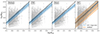 |
Fig. 4. Scatter plot for WL mass point estimates of DEMNUni-Cov clusters. Error bars correspond to the standard deviation of the mean (in the mean/ML panels), 16th and 84th percentiles (in the median panel), or SBI (in the CBI pannel). The one-to-one line is shown in black, while blue lines give results for the linear regression over the data points for the ‘LSS + shape noise’ case. The orange line shows the linear regression for ML WL mass measured on DEMNUni-Cov data with the combination of systematic effects discussed in Sect. 7. The shaded region corresponds to the scatter. |
To better evaluate the level of WL mass accuracy and precision, we perform a linear regression of the true mass versus the WL mass point estimate using the LIRA (LInear Regression in Astronomy, Sereno 2016) package. Intercept α, slope β, and intrinsic scatter σ are calculated from the linear regression of the logarithmic masses as

where the pivot mass is Mpiv = 1014 M⊙. Results are presented in Table B.1. The slope and intercept values indicate how close the regression line is to a one-to-one relationship, and thus account for the accuracy. The scatter quantifies how close the mass dependence is to the linear relation in Eq. (22), and thus accounts for the precision.
The ML is the most accurate point estimate for the overall mass range (β ∼ 1). Given the adopted priors, the bias is mass dependent for the mean, median, or CBI estimators, (β ∼ 0.9). In the low-mass regime, the mean, median, or CBI estimators are accurate, but significantly deviate from the one-to-one relation at higher cluster masses. The scatter of the ML masses is about twice the size of that from the other statistical estimators, which makes the ML masses less precise.
The level of precision of the different estimators can be strongly impacted by the mass prior. The ML estimator is by design not affected by the shape of the prior but it is still affected by the lower limit of the fitted parameter space. At low masses, the prior can play a stabilising role. For low or negative (S/N)WL, the ML estimator is very close to the minimum considered mass, log MWL = 13. In our analysis, 18.9% of the ML estimates reach the lower limit of the mass range. On the other hand, even when the peak of the mass posterior probability is at very low masses, the median, CBI, or mean estimators better account for the tail of the distribution at larger masses, and hence have a significantly lower scatter.
4.2.2. Mass bias
To quantify the WL mass accuracy, we can look at the mass bias, that is the ratio between the WL mass and the true halo mass,
To first-order in the Taylor expansion, the mass bias can be written as
Hereafter, all references to the mass bias correspond to the definition in Eq. (24).
The ensemble average mass bias ⟨bM⟩, which measures the accuracy, and the related scatter σb, which measures the precision, are computed as in Eqs. (20), (21), respectively. We calculate the uncertainty of mass bias and scatter estimates as the standard deviation of 1000 bootstrap realizations.
Figure 5 shows the weighted average of the mass bias in 8 equispaced logarithmic mass bins. The WL mass for low-mass clusters is underestimated. This is particularly severe for median, CBI, and mean point estimates, for which the WL mass, in the mass range 14 ≲ log Msim ≲ 14.5, is about 50% of the true mass. On the other hand, the ML mass suffers from a less severe bias, and, for the same mass bins, it is no less than 80% of the true mass on average. For massive clusters, the bias is smaller. However, in the high-mass range, the number of simulated clusters is low and the bias measurement is strongly affected by statistical fluctuations.
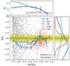 |
Fig. 5. Weighted average (plotted as lines) of the WL mass bias for median, CBI, mean, and ML point estimates as a function of the true mass of the DEMNUni-Cov clusters. The grey points show the WL mass bias for ML estimates. Results from ECG are presented with red lines and points. The light and dark yellow bands mark ±10% and 20% thresholds, respectively. Top and right panels give the mass bias scatter and the distribution of the mass bias points for each estimator, respectively. Error bars are the standard deviation of the bootstrap sample distribution of weighted means. |
The intrinsic scatter decreases as the cluster mass increases. In the low-mass regime, the scatter of the ML masses is larger than the scatter of the median, CBI, or mean measurements. This difference vanishes for higher masses, where the (S/N)WL can become significant.
Table B.2 provides the weighted mean of the WL mass bias for each point estimate. Median, CBI, and mean data points underestimate the true mass by approximately 23–27%, while ML masses are on average more accurate, ⟨bM⟩= − 14.6%. For the overall mass range, the scatter is mainly driven by the numerous, low-mass haloes, and it is larger for the ML mass, which can often coincide with the lower limit of the parameter space. The scatter reduces from 1.07 to 0.83 when only considering objects with ML mass strictly larger than the lower limit of the mass prior. On the other hand, the scatter of high-mass clusters is lower and nearly independent of the point estimate of the mass, see Fig. 5.
In summary, for the prior we considered, the ML mass is more accurate but less precise than median, CBI, or mean masses. The precision of the ML is similar to other point estimates in the high-mass regime, log Msim ≳ 14.5. The results may depend on priors, which should be optimised for each analysis based on the scientific goal.
4.3. Comparison with the Three Hundred
The mass bias of the Three Hundred clusters is smaller than the bias of the DEMNUni-Cov clusters, which cover a larger mass and redshift range, see Fig. 1. A fair comparison requires one to consider the mass bias of the 318 DEMNUni-Cov clusters within the mass range of the 3 × 324 Three Hundred clusters.
In Fig. 6, we show the weighted mean of the mass bias and associated scatter for clusters with true mass Msim > Mmin, where log Mmin ≥ 14.4 is the lower limit of the cluster mass range. The WL mass bias for the ML estimator is in agreement regardless of the lower limit considered, while other statistical estimators agree for clusters with log Msim ≳ 14.7. Our mass bias scatter is about twice the scatter for the Three Hundred clusters, but the bias scatter values agree at the high-mass end. The difference can be explained in terms of the simulation settings. The distribution of the Three Hundred clusters better samples the high-mass end of the halo mass function, whereas the DEMNUni-Cov cluster mass distribution follows the halo mass function, thus predominantly populating the low-mass range. There are numerous DEMNUni-Cov objects with log Msim ≤ 14.7, 269 out of 318, which increase the mass bias when calculating the mean of the full sample. Conversely, the contribution of the 66 Three Hundred clusters (out of 972) has less impact on the mass bias. Furthermore, ECG focus on the main halo and only consider particles in a slice of depth ± 5 Mpc in front of and behind the cluster. On the other hand, the DEMNUni-Cov settings fully account for correlated matter around the halo and uncorrelated matter from LSS, which is a significant source of scatter awt the Euclid lensing depth Euclid Collaboration: Sereno et al. 2024.
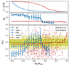 |
Fig. 6. Weighted average of the WL mass bias of DEMNUni-Cov clusters with Msim > Mmin as a function of Mmin. Results are compared with measurements performed on the Three Hundred cluster sample from ECG. Top panels give the fraction of clusters in the considered mass range (top) and the mass bias scatter (middle). The vertical line is at log Mmin = 14.7 lower limit. Error bars are the standard deviation of the bootstrap sample distribution. |
Averaged density profiles and measured masses for log Msim ≥ 14.7 are shown in Fig. 2 and reported in Table 1, respectively. The agreement with the Three Hundred results is also found in the analysis of the linear regression of the true mass versus the median WL mass, see Fig. 7. We use the median to be consistent with ECG, which measures the 16th, 50th, and 84th percentiles of the mass. The parameters fitted to the DEMNUni-Cov clusters are α = −0.136 ± 0.064 and β = 1.146 ± 0.099, while those for the Three Hundred are α = −0.114 ± 0.046 and β = 1.081 ± 0.044. However, consistently with the scatter of the weighted average, our measured scatter from the linear regression is about two to three times larger than that of the Three Hundred, σ = 0.158 ± 0.018 vs. σ = 0.064 ± 0.003. We attribute this to the different mass distribution of objects, and to the uncorrelated LSS noise in the shear.
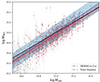 |
Fig. 7. Scatter plot for median WL mass point estimates of DEMNUni-Cov clusters in the ECG mass range. Error bars correspond to the 16th and 84th percentiles. The red line shows the linear regression for median WL mass measured in ECG. The shaded region corresponds to the scatter. |
5. Assessment of systematic effects in lens or source catalogues
The analysis in Sect. 4 presents cluster mass measurements in an idealised setting where lens and source catalogues are unbiased and where only sources of intrinsic scatter and noise, such as LSS and shape noise, triaxiality, or cluster orientation, play a role. In this section, we test how well WL mass can be measured and how observational and measurement effects impact WL mass measurements. In particular, we examine the effects of redshift uncertainty, selection effects from optical cluster detection algorithms, cluster centroid offsets, and masked data.
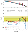 |
Fig. 8. Weighted average of the WL mass bias for the ML mass estimator. Data sets considered are ‘LSS + shape noise’ (Sect. 4), photo-z non-conservative selection (Sect. 5.1.1), photo-z robust selection (Sect. 5.1.2), AMICO-like sample (Sect. 5.2), PZWav-like sample (Sect. 5.2), masks (Sect. 5.3), BMO model (Sect. 6.1), and combined effects (Sect. 7). The top panel shows the mass bias scatter. Error bars are the standard deviation of the bootstrap sample distribution. |
To quantify the impact of each systematic effect, we define the relative mass change
where Mref is the reference WL mass measured in the unbiased ‘LSS + shape noise’ case as in the previous section, and Msys is the WL mass measured on catalogues with additional systematic effects. As in Eq. (24), we express the relative mass change in terms of the natural logarithm. We measure the ensemble average mass change, ⟨ΔlnM⟩, as given in Eq. (20) for clusters in common in reference and comparison samples. The error for this measurement is the standard deviation of the bootstrap sample distribution.
The mass shift can be further assessed with the WL mass measured by fitting the cluster ensemble averaged lensing profile, see Eq. (19), ΔlnM⟨ΔΣ⟩. All clusters of the samples are accounted in the averaged lensing profile. The uncertainty for ΔlnM⟨ΔΣ⟩ is the sum in quadrature of the standard deviations of the posterior distribution for both reference and comparison samples.
Table 3 lists the relative mass variation for the cluster mass ensemble average and the cluster lensing profile ensemble average. Figure 9 shows mass change for the cluster mass ensemble average in different mass bins.
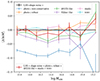 |
Fig. 9. Relative change of the WL mass with respect to the ‘LSS plus shape noise’ case due to systematic effects. We consider the ML estimator. Data sets considered are photo-z non-conservative selection (Sect. 5.1.1), photo-z robust selection (Sect. 5.1.2), AMICO-like sample (Sect. 5.2), PZWav-like sample (Sect. 5.2), masks (Sect. 5.3), BMO model (Sect. 6.1), and combined effects (Sect. 7). Error bars are the standard deviation of the bootstrap sample distribution. |
Relative change of the WL mass with respect to the ‘LSS plus shape noise’ case due to systematic effects.
Hereafter, we primarily present results on WL mass, mass bias, and relative mass change using ML point estimates. The ML point estimate is often considered in lensing analyses of Stage-III surveys or precursors (Euclid Collaboration: Sereno et al. 2024). Properties of each sample presented in this section are summarised in Table A.1.
5.1. Source redshift uncertainty
Measuring unbiased WL masses requires a robust identification of background galaxies. Contamination from foreground or cluster member galaxies substantially dilutes the lensing signal Melchior et al. 2017, thus increasing the WL mass bias towards negative values. We define the contamination fraction following Euclid Collaboration: Lesci et al. 2024 as
where p is the photo-z selection criterion, defined via Eq. (8) or Eq. (28), and Nsel is the number of galaxies selected with the condition p.
Contamination by cluster members could be corrected with a so-called ‘boost factor’, applied either directly to the shear data (e.g. Murata et al. 2018) or added to the mass model (e.g. McClintock et al. 2019). In this work, we do not include a boost factor to correct for signal dilution. In fact, we find, in agreement with Euclid Collaboration: Lesci et al. 2024, that a boost correction is not necessary if one applies a sufficiently conservative source selection. However, boosting the WL signal allows for effective correction of the lensing signal, resulting in accurate mass calibration (e.g. Varga et al. 2019).
Primary Euclid WL probes will divide galaxies into tomographic bins and perform a redshift calibration a posteriori to correct the galaxy distribution n(z) in each bin. Cluster WL masses can be measured considering tomographic bins for background source redshifts with the ensemble n(z) calibration (e.g. Bocquet et al. 2024; Grandis et al. 2024). Using tomographic bins can result in significant foreground contamination in the background galaxy sample. However, this can be corrected using a well-known and calibrated source redshift distribution.
To study the effects of source selection on cluster WL masses, we simulate observed photometric source redshifts, zobs, from the true source redshifts, ztrue,
We consider two source populations. The first population accounts for well-behaved photo-zs, whose deviations  follow a Gaussian distribution centred on a redshift bias
  and with scatter
  .
.
The second population accounts for catastrophic outliers with  , for which
  is uniformly distributed in the
  region up to zs = 3. The distribution of simulated photo-zs is shown in Fig. 10.
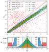 |
Fig. 10. Scatter plot of simulated photo-z vs. true redshift for non-conservative (red + blue) or robust (green − orange) selection. The bottom panel shows the marginalised 1D distribution of the normalised redshift deviation. |
The parameters of the distributions we use are informed by Euclid Collaboration: Bisigello et al. 2023, who measure photo-z bias and scatter from simulated Euclid data Bisigello et al. 2020 using various codes. Measurements of the photo-z bias are in agreement with those found for cosmic shear analyses Euclid Collaboration: Ilbert et al. 2021. The photometry is simulated for Euclid and Rubin/LSST bands with Gaussian noise. The photometric noise distributions depend on the survey depth and is fixed to one tenth of the flux corresponding to a S/N > 10.
Below, we describe our simulations of two different photo-z selected source samples, a non-conservative or a robust galaxy selection, and we examine the precision in lensing signal and mass in both scenarios. The distribution n(z) beyond the cluster redshift zd = 0.3, as well as the distribution n(z) of the original DEMUni-Cov sample, for both photo-z selections, are shown in Fig. 11.
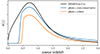 |
Fig. 11. Redshift distribution of DEMNUni-Cov sources, and of non-conservative and robust photo-z-selected sources beyond zd = 0.3. |
5.1.1. Non-conservative photo-z selection
Here, we consider the systematic uncertainty on cluster WL masses derived using a non-conservative source selection that selects background galaxies based only on the photo-z point estimate, without any further photo-z quality cuts. This is analogous to cluster WL with tomographic bins.
For this non-conservative selection, we expect the distribution of observed photo-zs to comprise a fraction of well-behaved galaxies with Gaussian scatter around the true redshift as well as a fraction of catastrophic outliers. Based on models of Euclid plus ground-based complementary photometry from Euclid Collaboration: Bisigello et al. 2023, and their analysis of HE-band detected galaxies with S/N > 3, we expect an outlier fraction of 12.7%. For the distribution of non-catastrophic, well-behaved photo-zs, we consider a normal distribution with mean  and dispersion
  . Figure 10 shows the distribution of simulated galaxy redshifts.
Sources are selected to be background galaxies following Eq. (8). As shown in Fig. 12, this simple selection criterion results in significant foreground source contamination. The contamination, as defined in Eq. (26), increases with the cluster redshift. This is because the total number of background sources reduces, while the number of contaminated sources increases with increasing redshift.
5.1.2. Robust photo-z selection
To reduce foreground contamination, we can make additional quality cuts in the galaxy source sample, for example, requiring that the photo-z probability distribution is well behaved with a prominent peak, or that a significant fraction of the distribution is above the lens redshift Sereno et al. 2017. These conservative cuts can significantly reduce the systematic contamination at the expense of a slightly smaller sample of selected galaxies and a slightly higher noise level Euclid Collaboration: Lesci et al. 2024.
We model the properties of the robustly selected galaxies as follows. Firstly, we conservatively assume that reliable shapes and nearly unbiased photo-zs can be measured for about 70% of the full galaxy population (e.g. Bellagamba et al. 2012, 2019; Ingoglia et al. 2022), and, therefore, we randomly discard 30% of the galaxies from the sample. Euclid and Stage-IV surveys should perform even better in terms of completeness Euclid Collaboration: Lesci et al. 2024.
Next, we assume that after applying redshift quality cuts, we are left with galaxies with a well-behaved, single peaked photo-z probability density distribution whose signal is likely better detected than for the full sample. Consequently, we model the observed photo-z distribution of the selected sources as galaxies expected to be observed in HE-band images with S/N > 10 Euclid Collaboration: Bisigello et al. 2023. We expect 4% of outliers, but we do not include these objects in the sample as we assume that their fraction is significantly reduced to the sub-percent level thanks to the robust photo-z selection, possibly coupled with thorough colour selections as discussed in Euclid Collaboration: Lesci et al. 2024. Deviations from the true redshifts of these photo-zs are normally distributed with mean  and dispersion
  . Figure 10 shows the redshift distribution of the robustly selected galaxies.
Finally, we select galaxies according to the robust criterion Sereno et al. 2017
where zs, min is the  lower limit of the galaxy photo-z distribution. Figure 12 shows that the robust selection significantly reduces the foreground contamination of the source sample.
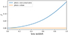 |
Fig. 12. Photo-z contamination fraction as a function of the lens redshift of non-conservative or robust photo-z selected sources. |
5.1.3. Impact of photo-z uncertainties
In Fig. 13, we plot the difference between the (S/N)WL for the ‘LSS + shape noise’ source catalogue with true galaxy redshifts, see Fig. 3, and that derived from a source catalogue with photo-z noise. Photo-z noise generally reduces the lensing (S/N)WL, particularly in the higher-mass bins. The reduction is larger for the non-conservative photo-z selected sample, with (S/N)WL lower by 15% on average, than for the robust one, (S/N)WL lower by 5% on average. We notice a larger (S/N)WL using the robust selection in some high-mass, high-redshift bins. However, their low statistics do not allow for a significant conclusion about deviations from the ‘LSS + shape noise’ case. As summarised in Table 2, photo-z noise generally decreases the (S/N)WL. The decrease is slightly smaller in the robust case because the removal of foreground contaminants strengthens the lensing signal. However, at low mass and low redshift, the robust photo-z selection decreases the (S/N)WL slightly more than in the non-conservative case. This is because the robust photo-z cut reduces the overall number of sources and shape noise dominates in this mass regime.
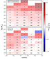 |
Fig. 13. Difference of the (S/N)WL as measured either for lensing with true redshifts, that is the ‘LSS + shape noise’ case, or non-conservative (top) or robust (bottom) photo-z selected samples, computed as the CBI of the values binned in mass and redshift. The number of clusters is displayed in each bin. |
Figure 8 shows the weighted average of the mass bias and scatter in different mass bins considering the ML point estimator. In the non-conservative case, the mass bias can be as large as −40% and it exceeds the −20% limit for log Msim ≲ 14.75. On the other hand, for the robustly selected background sample, the mass bias does not significantly change from the fiducial case. This trend is also seen for the relative mass change in Fig. 9, where the WL mass for the non-conservative selection differs from the WL mass measured on true redshift data. On the other hand, the robust photo-z selection does not show a significant relative change.
The mass bias and scatter averaged over the full sample mass range are summarised in Table B.2. The measured WL mass bias for the non-conservative photo-z selection is on average −34.4 ± 1.6%. On the other hand, the mass bias for the robust photo-z selection is very close to the unbiased measurement, ⟨bM⟩= − 14.6 ± 1.9%, but has a larger scatter due to the lower number of sources selected.
These results are consistent with the linear regression analysis, see Table B.1. The slope and intercept of the linear regression for the non-conservative selection are lower than in the unbiased sample, whereas the scatter is not significantly different. On the other hand, results for the robust photo-z selection are very similar to the unbiased case except for the scatter that is larger, in agreement with results from the mass bias.
The cluster average density profiles plotted in Fig. 2 further support our finding that non-conservative source selection significantly biases cluster WL measurements. On the other hand, we find that the average shear profiles of sources selected in the robust photo-z case are consistent with the ‘LSS + shape noise’ case.
Masses recovered from the average density profiles are given in Table 1 and the corresponding relative mass change is reported in Table 3. The mass is 22.3 ± 1.5% lower than the ‘LSS + shape noise’ case for the non-conservative selection, but differs by just 0.7 ± 1.7% for the robust photo-z selection.
The mass change as derived from the ensemble average of individual WL masses is −8.0 ± 0.2% for the non-conservative selection. This is due to the effect of the mass prior on noisy individual estimates.
To summarise, we find that the WL mass measurement can be significantly impacted by source redshift uncertainties without further calibration. However, this effect can be significantly mitigated with a careful source selection. A robust selection in photo-z to reduce foreground contamination can be coupled with a colour-colour selection to increase source completeness while preserving purity Euclid Collaboration: Lesci et al. 2024. Another possibility is to use calibrated redshift distributions from tomographic bins for cosmic shear along with an empirical correction for cluster member contamination Bocquet et al. 2024.
5.2. Cluster detection
Cluster detection can be another source of WL mass systematic effects, due to, for example, selection effects or miscentring. In this section, we study the potential impact of the optical cluster detection algorithms that will be used in the Euclid data analysis pipeline: the Adaptive Matched Identifier of Clustered Object algorithm AMICO Bellagamba et al. 2011, 2018; Euclid Collaboration: Adam et al. 2019, and the wavelet-based algorithm PZWav Gonzalez 2014; Euclid Collaboration: Adam et al. 2019; Thongkham et al. 2024. These two optical cluster finding algorithms are selected to run on Euclid data based on their performance in a comparative challenge of state-of-the-art detection algorithms Euclid Collaboration: Adam et al. 2019.
To construct simulated lens samples reflecting the expected performance of each algorithm in the Euclid survey, we first account for the cluster detection completeness. Euclid Collaboration: Cabanac et al. (in prep.) evaluates the performance of AMICO and PZWav by running them on the realistic simulated Euclid galaxy catalogue Flagship version 2.1.10 Potter et al. 2017; Euclid Collaboration: Castander et al. 2024. The completeness is calculated for galaxy clusters detected with (S/N)det > 3. In Fig. 14, we show the mass-redshift completeness of AMICO and PZWav. In each mass-redshift bin, we randomly pick DEMNUni-Cov galaxy clusters with an associated probability equal to the completeness of the bin. Following this procedure, we obtain two Euclid-like cluster samples, whose distributions are shown in Fig. 1. The sizes of the AMICO and PZWav-like catalogues are similar, 4557 and 4954 clusters, respectively.
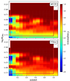 |
Fig. 14. Expected completeness for the AMICO and PZWav algorithms as a function of mass and redshift. The light red box encloses the parameter space sampled by the DEMNUni-Cov haloes. |
To simulate realistic cluster catalogues, we take into account the centroid offset, that is the angular separation between the true cluster centre and the location of the detection, and realistic cluster redshifts based on the performance of the algorithms Euclid Collaboration: Adam et al. 2019. We randomly shift the centre positions of AMICO-like (PZWav-like) clusters on the perimeter of a circle centred on the true position using a separation following a log-normal distribution with a mean of  and RMS
  Euclid Collaboration: Adam et al. 2019. Figure 15 displays the centroid offset distribution generated for each cluster detection algorithm. Redshifts of detected clusters are scattered as
  for masses lower than 1014 M⊙, and
  for masses larger than 1014 M⊙.
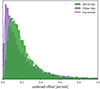 |
Fig. 15. Centroid offsets of AMICO-like and PZWav-like clusters selected from the DEMNUni-Cov catalogue. |
We show the weighted average of the mass bias of Euclid-like clusters in Fig. 8. For both samples, the mass bias is generally larger than for the full DEMNUni-Cov catalogue, which is well-centred and complete. The impact on the mass bias seems larger in the low-mass range, where AMICO-like and PZWav-like samples are less complete. The mass bias of PZWav-like clusters is larger than for AMICO-like clusters due to the larger dispersion of the centroid offset.
Table B.2 presents the results of the ensemble average mass bias and scatter. For the two detection algorithms and in comparison with results presented in Sect. 4, WL mass bias values are slightly more severe. AMICO (PZWav) clusters have a WL mass that is lower than the true mass on average by 18.2 ± 2.0% (21.0 ± 2.0%). The results of the linear regression presented in Table B.1 agree. For both Euclid-like samples, intercept and slope parameters are lower than parameters for the unbiased cluster sample, whereas the intrinsic scatter slightly increases. Uncertainties in cluster redshift and position lower the precision of the lensing mass.
Table 3 shows the relative change in WL mass. The ensemble WL mass change is not significantly impacted by systematic effects. The relative change given in WL mass as inferred from the averaged lensing signal, as shown in Fig. 2, is 5.3 ± 1.7% (0.9 ± 1.9%) larger for AMICO-like (PZWav-like) samples.
Cluster samples discussed here are selected from the DM haloes in the DEMNUni-Cov simulation given the expected performance of the Euclid detection algorithms, and we could not account for correlation between WL mass and optical proxies. Nevertheless, it is also known that optical cluster selection leads to WL selection biases Wu et al. 2022; Zhang & Annis 2022. This is due to secondary selection effects of optical clusters, like a preference for concentrated haloes, haloes aligned along the line of sight, and haloes with more structure along the line of sight, leading to projection effects in the measured richness.
An alternative approach would be to perform an end-to-end mass bias analysis with the large Euclid-like Flagship simulation Potter et al. 2017; Euclid Collaboration: Castander et al. 2024, including galaxy clusters directly detected with AMICO and PZWav. However, no shear products were available in Flagship at the time that the analysis presented in this paper was carried out.
5.3. Masks effects
Masking of data plays a major role in large surveys. Regions of the sky must be masked due to, for example, foreground bright stars. Masks lower the number of sources useful for WL, and increase the noise Liu et al. 2014. To consider these effects, we apply the binary mask of Pires et al. 2020, shown in Fig. B.1, to our catalogue. The mask is derived from Euclid simulated catalogues Euclid Collaboration: Desprez et al. 2020 using the code FLASK Xavier et al. 2016. The fraction of the masked sky is 22.4%, both on source and lens catalogues.
The resulting mass bias is shown in Fig. 8 and Table B.2. On the overall mass range, we do not see a significant difference with respect to the full-sky case with no masks, but we see a slightly larger scatter. The parameters of the linear regression, see Table B.1, are not significantly impacted. The relative mass change with respect to the unmasked case, see Table 3, is not statistically significant.
Here clusters are selected within the unmasked regions. On real data sets, cluster detection algorithms run on fields with masks. One way to assess WL mass precision and accuracy more realistically would be to detect clusters directly on masked mocks. In this way, we would also account for galaxy clusters detected at the edges of the mask.
6. Halo density model and priors
Here, we discuss the bias related to the fitting procedure adopted to derive the mass, in particular, the assumed model of the halo density profile and the role of priors.
6.1. BMO profile
The NFW profile has a non-physical divergence of its total mass Takada & Jain 2003. The BMO profile, a smoothly truncated version of the NFW profile, see Eq. (13), circumvents this problem, but it still suffers from the well-known degeneracy between mass and concentration. A halo with WL mass biased low can still fit the data if the concentration is biased high.
The BMO modelling gives results similar to NFW in terms of mass point estimators with respect to the true mass, see Table B.2 and Fig. 8. However, the WL mass and concentration inferred by fitting the averaged lensing signal are impacted. The BMO profile provides a better fit to the data at larger radii than the NFW profile, see Fig. 2, with a smaller reduced χ2, see Table 1. As shown in Table 3, the mass fitted to the averaged lensing profile is 5.1 ± 1.6% higher, while the concentration is 42.8% lower, which echoes the mass-concentration degeneracy existing for the NFW profile.
An additional step to further this analysis would be to consider the two-halo term. On larger scales than those reached in this study, that is  , the lensing signal of the halo is dominated by correlated matter, such as neighbouring haloes or filaments Tinker et al. 2005, 2010; Ingoglia et al. 2022.
6.2. Gaussian mass prior
To explore the role of the model, we consider an informative prior on the mass. We repeat the Bayesian analysis, and we fit the WL signal to a BMO profile with a Gaussian prior on the mass, which, combined with the prior limits set in Sect. 3.2.2, mimics the distribution of the DEMNUni-Cov clusters, see Fig. 1. The mean of the Gaussian prior is set to the mode of the cluster mass distribution. The dispersion is twice the standard deviation, so that the tail in the distribution towards high masses is accounted for. The prior is then truncated at the parameter limits.
The slope, intercept, and scatter of the linear regression between WL and true masses are reported in Table B.1. By definition, the prior does not affect the ML analysis, but it affects results for point estimators based on the posterior probability distribution. For the median, CBI, and mean point estimates, the slope and intercept parameters are lower than for the fiducial setting with a uniform prior. The intrinsic scatter is also two times lower. The informative prior leads to increased precision but also to a larger bias.
Results of the analysis of the weighted mass bias, see Table B.2, are consistent with those of the linear regression. The mass bias is more severe but the scatter is lower for the median, CBI, and mean WL mass leading to a decreased accuracy and increased precision. Other prior functions could also be explored, in particular priors based on mass-concentration relations (e.g. Meneghetti et al. 2014; Diemer & Kravtsov 2015; Diemer & Joyce 2019; Euclid Collaboration: Giocoli et al. 2024).
7. Accuracy and precision in an Euclid-like survey
Finally, to provide a preliminary overview of the accuracy and precision we can expect from WL mass measurements in Euclid, we measure the mass bias and the relative mass change considering at the same time all the systematic effects previously discussed. To mimic a realistic scenario Euclid Collaboration: Sereno et al. 2024, we consider the following setting:
-
robust photo-z source selection (Sect. 5.1.2);
-
AMICO-like clusters (Sect. 5.2);
-
masked catalogues (Sect. 5.3);
-
BMO halo profile and Gaussian prior (Sect. 6).
In terms of precision of the lensing signal, we find 140 (about 3.9%) clusters with (S/N)WL > 3, similar to the fraction of clusters with (S/N)WL > 3 measured from catalogues in the ‘LSS + shape noise’ case (about 3.7%). In terms of precision of the recovered WL mass, the scatter as inferred either from the linear regression of the ML mass or the weighted average analysis is larger than the scatter of the ‘LSS + shape noise’ case if we consider the ML point estimate. However, looking at the median, CBI, or mean point estimates, the scatter is smaller and the precision is increased, mainly due to the Gaussian mass prior.
In terms of accuracy of the recovered WL mass, the slope and intercept values of the ML mass linear regression are statistically consistent with those of the ‘LSS + shape noise’ case, with intercept α = −0.097 ± 0.010 and slope β = 0.924 ± 0.043, see Fig. 4. For the median, CBI, and mean WL mass, the recovered accuracy is lower.
The weighted average mass bias is summarised in Table B.2. The ML mass is larger than 80% of the true mass in a significant mass range, see Fig. 8. The bias of the ML mass is ⟨bM⟩= − 15.4 ± 2.5% for the full sample. The median, CBI, and mean estimators exhibit a larger increase in mass bias with respect to the ‘LSS + shape noise’ case measurement than the ML estimator. Looking at the relative mass change, see Table 3, we find that the ensemble average ML mass is consistent with the ‘LSS + shape noise’ case, suggesting that systematic effects can be well controlled.
The difference in the average lensing profile is due to the effect of the selection function of Euclid detected clusters. In the low-mass regime, clusters are not detected and the ensemble average of the cluster surface mass density profile increases compared to the profile of the full cluster population. A residual difference in the fitted mass is due to the BMO halo density model compared to NFW.
8. Summary
To exploit the full cosmological constraining power of galaxy clusters, their WL masses must be well characterised. This requires testing the accuracy and precision of algorithms for WL mass measurement on simulated data. We can then use the resulting mass bias measurements to understand the impact of systematic effects on cluster WL masses.
In view of the first data from the Euclid survey, we investigate the mass bias with COMB-CL, the Euclid pipeline for cluster WL mass measurements. Using COMB-CL on the DEMNUni-Cov N-body simulations, we study the WL mass of 6155 clusters with true mass Msim > 5 × 10¹³ M⊙ (or log Msim ≳ 13.7) and redshift zd < 1.
We first assess the precision and accuracy of the measured shear profile and WL mass in an ideal scenario with no measurement errors or uncertainties, but where the measured mass can differ from the true one due to, for example, shape noise, LSS, triaxiality, and cluster orientation, mergings or irregular morphology Euclid Collaboration: Ajani et al. 2023. This allows us to quantify the intrinsic bias and scatter of the WL mass with respect to the true cluster mass. We summarise the results discussed in Sect. 4 as follows.
-
The lensing signal of low-mass clusters is expected to be low. Only 3.7% of the clusters are recovered with (S/N)WL > 3, most of which lie at the sparsely populated, high-mass end. We find agreement with the semi-analytical forecasting presented in Euclid Collaboration: Sereno et al. 2024.
-
The mass bias significantly depends on the mass point-estimator of choice. A summary statistic with only a location and a scale might be not enough to properly describe the mass probability function of a halo with low (S/N)WL. We measure the average mass bias via four statistical estimators: median, biweight location (CBI), mean, and maximum likelihood (ML). We find that the ML point estimate yields a WL mass almost two times more accurate than those of the median, CBI, and mean. In fact, at low masses, the mass bias can be as large as ⟨bM⟩∼ − 40%. The ML point estimate is more accurate, with ⟨bM⟩≳ − 20% in the full mass range. For the full sample, the WL mass is on average biased low by about 23.5–26.7 ± 1.2% for median, CBI, and mean measurements, and 14.6 ± 1.7% for ML. However, the intrinsic scatter of the ML masses is about two times larger than other mass estimates.
-
At the massive end of the halo mass function, log Msim ≥ 14.7, we find a mass bias in agreement with that measured with the massive Three Hundred clusters Euclid Collaboration: Giocoli et al. 2024. Our sample extends to lower masses and larger redshifts, as expected for Euclid-like clusters. We find that the bias over the full mass range is three to five times larger than that measured for massive clusters. The larger scatter in the DEMNUni-Cov sample is due to noise by correlated matter or LSS.
We go beyond the simple scenario with only intrinsic scatter and noise and check how various systematic effects or uncertainties, such as photo-z uncertainties, sample incompleteness, or masks, affect the WL mass measurements. We mostly focus on the ML mass estimator. Results are discussed in Sect. 5 and summarised below.
-
Following Euclid Collaboration: Bisigello et al. 2023, we simulate observed galaxy photometric redshifts in two different scenarios, a robust photo-z sample, with a conservative source selection, and a non-conservative photo-z sample, which suffers from significant contamination or photo-z outliers. For the non-conservative selection, which is similar to WL analyses in tomographic bins, we find that the lensing signal is biased low by 15%, and that the WL mass bias is −33.4 ± 1.6% on the overall cluster mass range. For the robust selection, the lensing signal and the WL mass are well recovered over the full cluster mass range with a mass bias of −14.7 ± 1.9%.
-
We simulate Euclid-like cluster samples considering the two cluster detection algorithms selected to run in the Euclid analysis pipeline, AMICO and PZWav Euclid Collaboration: Adam et al. 2019. Each sample is simulated with the corresponding completeness, centroid offset distribution, and redshift uncertainty. Thanks to the high completeness, Euclid samples will recover the full halo population even in the low-mass regime, even though miscentering and redshift uncertainty could dilute the lensing signal. The relative change of the measured WL mass with respect to the true WL mass is on average −1.5(−2.5)±0.3% for AMICO (PZWav)-like clusters.
-
We apply masks to the simulated data and find that the resulting WL masses remain consistent with the ideal scenario, even though some constraining power is lost due to the lower number of selected background galaxies.
We additionally consider the effects of halo profile modelling and priors.
-
We switch the NFW model of the halo density profile to a BMO profile. On average, individual WL masses are consistent with mass measured with a NFW profile. We notice that the BMO model better describes the averaged lensing profile, with a lower reduced χ2. On averaged density profiles, the BMO profile brings the WL mass higher, with a relative change with respect to the NFW WL mass of 5.1 ± 1.6%.
-
The prior affects the median, CBI, and mean mass point estimates. With a Gaussian prior on the mass, the scatter on the mass is two times lower and the bias more severe than for a uniform prior, leading to a higher precision and a lower accuracy.
A final test is performed using a combination of the aforementioned effects including masks and realistic photo-zs.
-
We consider AMICO-like clusters, detected in the presence of masks, with robustly selected source galaxies. We fit a BMO model with a Gaussian mass prior. From the linear regression of the WL mass – true mass relation, we find a higher scatter than for the fiducial case with only instinsic scatter and noise, but a similar accuracy as measured with the slope and intercept parameters. Thanks to the high completeness of the lens sample and the robust source selection, the average mass bias, ⟨bM⟩= − 15.5 ± 2.4%, agrees with that expected in an ideal scenario.
9. Discussion
Our analysis considers a broad selection of systematic effects, including triaxiality and cluster orientation, LSS and shape noise, source redshift uncertainties, and detection uncertainties from cluster-finding algorithms. However, in this work, we do not consider calibration of the spurious lensing signals induced by improper shear measurements or blended objects. Shear correction calibrated for cosmic shear may not be appropriate in the cluster regime since the shear response can become non-linear for stronger shears Hernández-Martín et al. 2020. Further improvements to the methodology and a full calibration of the cluster mass bias would require realistic cluster image simulations. Moreover, we do not account for intrinsic alignment and the clustering of sources, which are subdominant for single cluster WL mass analyses (e.g. Chisari et al. 2014).
The analysis presented in this paper assumes that the miscentring of galaxy clusters follows an isotropic distribution. This approximation accounts for random deviations from the gravitational centre but does not consider inherent (directional) correlations between the centre proxy and WL shear measurements. Such correlations might arise, for example, when cluster centres are identified based on properties of the intracluster medium, as discussed in Sommer et al. 2024.
We characterise WL mass bias using point estimates, simplifying the treatment by neglecting posterior shapes. As Lee et al. 2018 show, bias and scatter can be derived using the full posterior of the WL mass measurement. This approach provides a close approximation (∼4% relative difference) to our mean point estimate.
Cluster WL mass bias could be further reduced with improvements to the halo density model. We find that fitting improves if we consider a truncation radius. Proper modelling for miscentring, concentration, or correlated or infalling matter could further improve the fit Bellagamba et al. 2019; Giocoli et al. 2021; Ingoglia et al. 2022.
We underline that this study is part of a larger series of work to characterise cluster WL masses with Euclid. Euclid Collaboration: Sereno et al. 2024 tests the robustness of Euclid cluster mass measurement algorithms on an extensive data set of Stage-III surveys or precursors. Euclid Collaboration: Lesci et al. 2024 derives colour selections from Euclid and ground-based photometry to optimise the quality of the WL signal. Ongoing testing and future works will exploit the Flagship simulation Potter et al. 2017; Euclid Collaboration: Castander et al. 2024 to perform a complete end-to-end cluster WL analyses within Euclid.
https://gitlab.euclid-sgs.uk/PF-LE3-CL/LE3_COMB_CL The access is restricted to members of the Euclid Consortium. A public release is expected with Euclid Collaboration: Farrens et al. (in prep.).
Acknowledgments
The Euclid Consortium acknowledges the European Space Agency and a number of agencies and institutes that have supported the development of Euclid, in particular the Agenzia Spaziale Italiana, the Austrian Forschungsförderungsgesellschaft funded through BMK, the Belgian Science Policy, the Canadian Euclid Consortium, the Deutsches Zentrum für Luft- und Raumfahrt, the DTU Space and the Niels Bohr Institute in Denmark, the French Centre National d’Etudes Spatiales, the Fundação para a Ciência e a Tecnologia, the Hungarian Academy of Sciences, the Ministerio de Ciencia, Innovación y Universidades, the National Aeronautics and Space Administration, the National Astronomical Observatory of Japan, the Netherlandse Onderzoekschool Voor Astronomie, the Norwegian Space Agency, the Research Council of Finland, the Romanian Space Agency, the State Secretariat for Education, Research, and Innovation (SERI) at the Swiss Space Office (SSO), and the United Kingdom Space Agency. A complete and detailed list is available on the Euclid web site (https://www.euclid-ec.org/). LI and MS acknowledge financial contributions from INAF Theory Grant 2023: Gravitational lensing detection of matter distribution at galaxy cluster boundaries and beyond (1.05.23.06.17). LI acknowledges financial support from the INAF grant 2023: Testing the origin of giant radio halos with joint LOFAR (1.05.23.05.11). MS acknowledges financial contributions from contract ASI-INAF n.2017-14-H.0 and contract INAF mainstream project 1.05.01.86.10. LI and LM acknowledge the grants ASI n.2018- 23-HH.0 and ASI n. 2024-10-HH.0 “Attività scientifiche per la missione Euclid – fase E”. LM acknowledges the grant ASI n.I/023/12/0. GC thanks the support from INAF theory Grant 2022: Illuminating Dark Matter using Weak Lensing by Cluster Satellites, PI: Carlo Giocoli. GC and LM thank Prin-MUR 2022 supported by Next Generation EU (n.20227RNLY3 The concordance cosmological model: stress-tests with galaxy clusters). The DEMNUni-cov simulations were carried out in the framework of “The Dark Energy and Massive Neutrino Universe covariances" project, using the Tier-0 Intel OmniPath Cluster Marconi-A1 of the Centro Interuniversitario del Nord-Est per il Calcolo Elettronico (CINECA). We acknowledge a generous CPU and storage allocation by the Italian Super-Computing Resource Allocation (ISCRA) as well as from the coordination of the “Accordo Quadro MoU per lo svolgimento di attività congiunta di ricerca Nuove frontiere in Astrofisica: HPC e Data Exploration di nuova generazione”, together with storage from INFN-CNAF and INAF-IA2. GD acknowledges the funding by the European Union – NextGenerationEU, in the framework of the HPC project – “National Centre for HPC, Big Data and Quantum Computing” (PNRR – M4C2 – I1.4 – CN00000013 – CUP J33C22001170001). LM acknowledges the financial contribution from the grant PRIN-MUR 2022 20227RNLY3 “The concordance cosmological model: stress-tests with galaxy clusters” supported by Next Generation EU and from the grants ASI n.2018-23-HH.0 and n. 2024-10-HH.0 “Attività scientifiche per la missione Euclid – fase E”.
References
- Abbott, T. M. C., Abdalla, F. B., Allam, S., et al. 2018, ApJS, 239, 18 [Google Scholar]
- Aihara, H., Arimoto, N., Armstrong, R., et al. 2018, PASJ, 70, S4 [NASA ADS] [Google Scholar]
- Allen, S. W., Evrard, A. E., & Mantz, A. B. 2011, ARA&A, 49, 409 [Google Scholar]
- Bahé, Y. M., McCarthy, I. G., & King, L. J. 2012, MNRAS, 421, 1073 [NASA ADS] [CrossRef] [Google Scholar]
- Baltz, E. A., Marshall, P., & Oguri, M. 2009, JCAP, 1, 015 [Google Scholar]
- Baratta, P., Bel, J., Gouyou Beauchamps, S., & Carbone, C. 2023, A&A, 673, A1 [NASA ADS] [CrossRef] [EDP Sciences] [Google Scholar]
- Bartelmann, M., & Schneider, P. 2001, Phys. Rep., 340, 291 [Google Scholar]
- Becker, M. R., & Kravtsov, A. V. 2011, ApJ, 740, 25 [NASA ADS] [CrossRef] [Google Scholar]
- Beers, T. C., Flynn, K., & Gebhardt, K. 1990, AJ, 100, 32 [Google Scholar]
- Bellagamba, F., Maturi, M., Hamana, T., et al. 2011, MNRAS, 413, 1145 [NASA ADS] [CrossRef] [Google Scholar]
- Bellagamba, F., Meneghetti, M., Moscardini, L., & Bolzonella, M. 2012, MNRAS, 422, 553 [Google Scholar]
- Bellagamba, F., Roncarelli, M., Maturi, M., & Moscardini, L. 2018, MNRAS, 473, 5221 [NASA ADS] [CrossRef] [Google Scholar]
- Bellagamba, F., Sereno, M., Roncarelli, M., et al. 2019, MNRAS, 484, 1598 [Google Scholar]
- Bisigello, L., Kuchner, U., Conselice, C. J., et al. 2020, MNRAS, 494, 2337 [NASA ADS] [CrossRef] [Google Scholar]
- Bocquet, S., Dietrich, J. P., Schrabback, T., et al. 2019, ApJ, 878, 55 [Google Scholar]
- Bocquet, S., Grandis, S., Bleem, L. E., et al. 2024, Phys. Rev. D, 110, 083509 [NASA ADS] [CrossRef] [Google Scholar]
- Borgani, S. 2008, in A Pan-Chromatic View of Clusters of Galaxies and the Large-Scale Structure, eds. M. Plionis, O. López-Cruz, & D. Hughes (Netherlands: Springer), 740, 24 [NASA ADS] [Google Scholar]
- Boyle, A., Uhlemann, C., Friedrich, O., et al. 2021, MNRAS, 505, 2886 [NASA ADS] [CrossRef] [Google Scholar]
- Carbone, C., Petkova, M., & Dolag, K. 2016, JCAP, 7, 034 [CrossRef] [Google Scholar]
- Castro, T., Quartin, M., Giocoli, C., Borgani, S., & Dolag, K. 2018, MNRAS, 478, 1305 [Google Scholar]
- Chisari, N. E., Mandelbaum, R., Strauss, M. A., Huff, E. M., & Bahcall, N. A. 2014, MNRAS, 445, 726 [NASA ADS] [CrossRef] [Google Scholar]
- Costanzi, M., Rozo, E., Simet, M., et al. 2019, MNRAS, 488, 4779 [NASA ADS] [CrossRef] [Google Scholar]
- Costanzi, M., Saro, A., Bocquet, S., et al. 2021, Phys. Rev. D, 103, 043522 [Google Scholar]
- Covone, G., Sereno, M., Kilbinger, M., & Cardone, V. F. 2014, ApJ, 784, L25 [NASA ADS] [CrossRef] [Google Scholar]
- Cropper, M., Cole, R., James, A., et al. 2012, in Space Telescopes and Instrumentation 2012: Optical, Infrared, and Millimeter Wave, eds. M. C. Clampin, G. G. Fazio, H. A. MacEwen, & J. M. Oschmann Jr., Society of Photo-Optical Instrumentation Engineers (SPIE) Conference Series, 8442, 84420V [NASA ADS] [CrossRef] [Google Scholar]
- Cropper, M., Hoekstra, H., Kitching, T., et al. 2013, MNRAS, 431, 3103 [Google Scholar]
- Cui, W., Knebe, A., Yepes, G., et al. 2018, MNRAS, 480, 2898 [Google Scholar]
- Cui, W., Dave, R., Knebe, A., et al. 2022, MNRAS, 514, 977 [NASA ADS] [CrossRef] [Google Scholar]
- de Jong, J. T. A., Verdoes Kleijn, G. A., Kuijken, K. H., & Valentijn, E. A. 2013, Exp. Astron., 35, 25 [Google Scholar]
- Diemer, B., & Joyce, M. 2019, ApJ, 871, 168 [NASA ADS] [CrossRef] [Google Scholar]
- Diemer, B., & Kravtsov, A. V. 2015, ApJ, 799, 108 [Google Scholar]
- Euclid Collaboration (Adam, R., et al.) 2019, A&A, 627, A23 [NASA ADS] [CrossRef] [EDP Sciences] [Google Scholar]
- Euclid Collaboration (Martinet, N., et al.) 2019, A&A, 627, A59 [NASA ADS] [CrossRef] [EDP Sciences] [Google Scholar]
- Euclid Collaboration (Blanchard, A., et al.) 2020, A&A, 642, A191 [NASA ADS] [CrossRef] [EDP Sciences] [Google Scholar]
- Euclid Collaboration (Desprez, G., et al.) 2020, A&A, 644, A31 [EDP Sciences] [Google Scholar]
- Euclid Collaboration (Ilbert, O., et al.) 2021, A&A, 647, A117 [NASA ADS] [CrossRef] [EDP Sciences] [Google Scholar]
- Euclid Collaboration (Moneti, A., et al.) 2022, A&A, 658, A126 [NASA ADS] [CrossRef] [EDP Sciences] [Google Scholar]
- Euclid Collaboration (Scaramella, R., et al.) 2022, A&A, 662, A112 [NASA ADS] [CrossRef] [EDP Sciences] [Google Scholar]
- Euclid Collaboration (Ajani, V., et al.) 2023, A&A, 675, A120 [NASA ADS] [CrossRef] [EDP Sciences] [Google Scholar]
- Euclid Collaboration (Bisigello, L., et al.) 2023, MNRAS, 520, 3529 [NASA ADS] [CrossRef] [Google Scholar]
- Euclid Collaboration (Giocoli, C., et al.) 2024, A&A, 681, A67 [NASA ADS] [CrossRef] [EDP Sciences] [Google Scholar]
- Euclid Collaboration (Lesci, G. F., et al.) 2024, A&A, 684, A139 [NASA ADS] [CrossRef] [EDP Sciences] [Google Scholar]
- Euclid Collaboration (Sereno, M., et al.) 2024, A&A, 689, A252 [NASA ADS] [CrossRef] [EDP Sciences] [Google Scholar]
- Euclid Collaboration (Castander, F., et al.) 2025, A&A, in press, https://doi.org/10.1051/0004-6361/202450853 [Google Scholar]
- Euclid Collaboration (Cropper, M., et al.) 2025, A&A, in press, https://doi.org/10.1051/0004-6361/202450996 [Google Scholar]
- Euclid Collaboration (Mellier, Y., et al.) 2025, A&A, in press, https://doi.org/10.1051/0004-6361/202450810 [Google Scholar]
- Foreman-Mackey, D., Hogg, D. W., Lang, D., & Goodman, J. 2013, PASP, 125, 306 [Google Scholar]
- Giocoli, C., Meneghetti, M., Bartelmann, M., Moscardini, L., & Boldrin, M. 2012, MNRAS, 421, 3343 [Google Scholar]
- Giocoli, C., Meneghetti, M., Metcalf, R. B., Ettori, S., & Moscardini, L. 2014, MNRAS, 440, 1899 [NASA ADS] [CrossRef] [Google Scholar]
- Giocoli, C., Metcalf, R. B., Baldi, M., et al. 2015, MNRAS, 452, 2757 [Google Scholar]
- Giocoli, C., Di Meo, S., Meneghetti, M., et al. 2017, MNRAS, 470, 3574 [NASA ADS] [CrossRef] [Google Scholar]
- Giocoli, C., Baldi, M., & Moscardini, L. 2018a, MNRAS, 481, 2813 [Google Scholar]
- Giocoli, C., Moscardini, L., Baldi, M., Meneghetti, M., & Metcalf, R. B. 2018b, MNRAS, 478, 5436 [Google Scholar]
- Giocoli, C., Marulli, F., Moscardini, L., et al. 2021, A&A, 653, A19 [NASA ADS] [CrossRef] [EDP Sciences] [Google Scholar]
- Gonzalez, A. 2014, Building the Euclid Cluster Survey– Scientific Program, Proceedings of a Conference Held July 6–11 2014 at the Sexten Center for Astrophysics, 7 [Google Scholar]
- Grandis, S., Mohr, J. J., Dietrich, J. P., et al. 2019, MNRAS, 488, 2041 [NASA ADS] [Google Scholar]
- Grandis, S., Bocquet, S., Mohr, J. J., Klein, M., & Dolag, K. 2021, MNRAS, 507, 5671 [NASA ADS] [CrossRef] [Google Scholar]
- Grandis, S., Ghirardini, V., Bocquet, S., et al. 2024, A&A, 687, A178 [NASA ADS] [CrossRef] [EDP Sciences] [Google Scholar]
- Gruen, D., Seitz, S., Becker, M. R., Friedrich, O., & Mana, A. 2015, MNRAS, 449, 4264 [NASA ADS] [CrossRef] [Google Scholar]
- Herbonnet, R., Crawford, A., Avestruz, C., et al. 2022, MNRAS, 513, 2178 [NASA ADS] [CrossRef] [Google Scholar]
- Hernández-MartÃn, B., Schrabback, T., Hoekstra, H., et al. 2020, A&A, 640, A117 [Google Scholar]
- Heymans, C., Van Waerbeke, L., Miller, L., et al. 2012, MNRAS, 427, 146 [Google Scholar]
- Hilbert, S., Barreira, A., Fabbian, G., et al. 2020, MNRAS, 493, 305 [Google Scholar]
- Hoekstra, H. 2003, MNRAS, 339, 1155 [NASA ADS] [CrossRef] [Google Scholar]
- Hoekstra, H., Mahdavi, A., Babul, A., & Bildfell, C. 2012, MNRAS, 427, 1298 [NASA ADS] [CrossRef] [Google Scholar]
- Hoekstra, H., Herbonnet, R., Muzzin, A., et al. 2015, MNRAS, 449, 685 [NASA ADS] [CrossRef] [Google Scholar]
- Ingoglia, L., Covone, G., Sereno, M., et al. 2022, MNRAS, 511, 1484 [NASA ADS] [CrossRef] [Google Scholar]
- Johnston, D. E., Sheldon, E. S., Tasitsiomi, A., et al. 2007, ApJ, 656, 27 [NASA ADS] [CrossRef] [Google Scholar]
- Kilbinger, M. 2015, Rep. Progr. Phys., 78, 086901 [Google Scholar]
- Knollmann, S. R., & Knebe, A. 2009, ApJS, 182, 608 [Google Scholar]
- Laureijs, R., Amiaux, J., Arduini, S., et al. 2011, arXiv e-prints [arXiv:1110.3193] [Google Scholar]
- Lee, B. E., Le Brun, A. M. C., Haq, M. E., et al. 2018, MNRAS, 479, 890 [Google Scholar]
- Lee, W., Cha, S., Jee, M. J., et al. 2023, ApJ, 945, 71 [NASA ADS] [CrossRef] [Google Scholar]
- Lewis, A., Challinor, A., & Lasenby, A. 2000, ApJ, 538, 473 [Google Scholar]
- Liu, X., Wang, Q., Pan, C., & Fan, Z. 2014, ApJ, 784, 31 [NASA ADS] [Google Scholar]
- Mantz, A. B., von der Linden, A., Allen, S. W., et al. 2015, MNRAS, 446, 2205 [Google Scholar]
- Marulli, F., Veropalumbo, A., & Moresco, M. 2016, Astron. Comput., 14, 35 [Google Scholar]
- McClintock, T., Varga, T. N., Gruen, D., et al. 2019, MNRAS, 482, 1352 [Google Scholar]
- Medezinski, E., Oguri, M., Nishizawa, A. J., et al. 2018, PASJ, 70, 30 [NASA ADS] [Google Scholar]
- Melchior, P., Gruen, D., McClintock, T., et al. 2017, MNRAS, 469, 4899 [CrossRef] [Google Scholar]
- Meneghetti, M., Rasia, E., Merten, J., et al. 2010, A&A, 514, A93 [NASA ADS] [CrossRef] [EDP Sciences] [Google Scholar]
- Meneghetti, M., Rasia, E., Vega, J., et al. 2014, ApJ, 797, 34 [Google Scholar]
- Miyazaki, S., Komiyama, Y., Kawanomoto, S., et al. 2018, PASJ, 70, S1 [NASA ADS] [Google Scholar]
- Murata, R., Nishimichi, T., Takada, M., et al. 2018, ApJ, 854, 120 [NASA ADS] [CrossRef] [Google Scholar]
- Murray, C., Bartlett, J. G., Artis, E., & Melin, J.-B. 2022, MNRAS, 512, 4785 [NASA ADS] [CrossRef] [Google Scholar]
- Navarro, J. F., Frenk, C. S., & White, S. D. M. 1996, ApJ, 462, 563 [Google Scholar]
- Navarro, J. F., Frenk, C. S., & White, S. D. M. 1997, ApJ, 490, 493 [Google Scholar]
- Oguri, M., & Hamana, T. 2011, MNRAS, 414, 1851 [NASA ADS] [CrossRef] [Google Scholar]
- Parimbelli, G., Anselmi, S., Viel, M., et al. 2021, JCAP, 1, 009 [NASA ADS] [Google Scholar]
- Parimbelli, G., Carbone, C., Bel, J., et al. 2022, JCAP, 11, 041 [Google Scholar]
- Peel, A., Pettorino, V., Giocoli, C., Starck, J.-L., & Baldi, M. 2018, A&A, 619, A38 [NASA ADS] [CrossRef] [EDP Sciences] [Google Scholar]
- Pires, S., Vandenbussche, V., Kansal, V., et al. 2020, A&A, 638, A141 [NASA ADS] [CrossRef] [EDP Sciences] [Google Scholar]
- Planck Collaboration VI. 2020, A&A, 641, A6 [NASA ADS] [CrossRef] [EDP Sciences] [Google Scholar]
- Planck Collaboration XXII. 2016, A&A, 594, A22 [NASA ADS] [CrossRef] [EDP Sciences] [Google Scholar]
- Potter, D., Stadel, J., & Teyssier, R. 2017, Comput. Astrophys. Cosmol., 4, 2 [NASA ADS] [CrossRef] [Google Scholar]
- Schäfer, B. M., Heisenberg, L., Kalovidouris, A. F., & Bacon, D. J. 2012, MNRAS, 420, 455 [Google Scholar]
- Schneider, P. 2006, in Saas-Fee Advanced Course 33: Gravitational Lensing: Strong, Weak and Micro, eds. G. Meylan, P. Jetzer, P. North, et al., 269 [Google Scholar]
- Schneider, P., van Waerbeke, L., Jain, B., & Kruse, G. 1998, MNRAS, 296, 873 [NASA ADS] [CrossRef] [Google Scholar]
- Seitz, C., & Schneider, P. 1997, A&A, 318, 687 [NASA ADS] [Google Scholar]
- Sereno, M. 2016, MNRAS, 455, 2149 [Google Scholar]
- Sereno, M., Covone, G., Izzo, L., et al. 2017, MNRAS, 472, 1946 [Google Scholar]
- Sereno, M., Giocoli, C., Izzo, L., et al. 2018, Nat. Astron., 2, 744 [NASA ADS] [CrossRef] [Google Scholar]
- Sommer, M. W., Schrabback, T., Applegate, D. E., et al. 2022, MNRAS, 509, 1127 [Google Scholar]
- Sommer, M. W., Schrabback, T., Ragagnin, A., & Rockenfeller, R. 2024, MNRAS, 532, 3359 [NASA ADS] [CrossRef] [Google Scholar]
- Springel, V., Wang, J., Vogelsberger, M., et al. 2008, MNRAS, 391, 1685 [Google Scholar]
- Takada, M., & Jain, B. 2003, MNRAS, 340, 580 [NASA ADS] [CrossRef] [Google Scholar]
- Tessore, N., Winther, H. A., Metcalf, R. B., Ferreira, P. G., & Giocoli, C. 2015, JCAP, 10, 036 [NASA ADS] [Google Scholar]
- Thongkham, K., Gonzalez, A. H., Brodwin, M., et al. 2024, ApJ, 967, 123 [NASA ADS] [Google Scholar]
- Tinker, J. L., Weinberg, D. H., Zheng, Z., & Zehavi, I. 2005, ApJ, 631, 41 [Google Scholar]
- Tinker, J. L., Robertson, B. E., Kravtsov, A. V., et al. 2010, ApJ, 724, 878 [NASA ADS] [CrossRef] [Google Scholar]
- Umetsu, K., Medezinski, E., Nonino, M., et al. 2014, ApJ, 795, 163 [NASA ADS] [CrossRef] [Google Scholar]
- Umetsu, K., Zitrin, A., Gruen, D., et al. 2016, ApJ, 821, 116 [Google Scholar]
- Umetsu, K., Sereno, M., Lieu, M., et al. 2020, ApJ, 890, 148 [NASA ADS] [CrossRef] [Google Scholar]
- Varga, T. N., DeRose, J., Gruen, D., et al. 2019, MNRAS, 489, 2511 [NASA ADS] [CrossRef] [Google Scholar]
- Vikhlinin, A., Kravtsov, A. V., Burenin, R. A., et al. 2009, ApJ, 692, 1060 [Google Scholar]
- Voit, G. M. 2005, Rev. Mod. Phys., 77, 207 [Google Scholar]
- Wu, H.-Y., Costanzi, M., To, C.-H., et al. 2022, MNRAS, 515, 4471 [CrossRef] [Google Scholar]
- Xavier, H. S., Abdalla, F. B., & Joachimi, B. 2016, MNRAS, 459, 3693 [NASA ADS] [CrossRef] [Google Scholar]
- Yang, X., Mo, H. J., van den Bosch, F. C., et al. 2006, MNRAS, 373, 1159 [Google Scholar]
- Zhang, Y., & Annis, J. 2022, MNRAS, 511, L30 [NASA ADS] [Google Scholar]
Appendix A: Samples properties
Properties of the different samples of the analysis.
Appendix B: Additional material
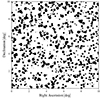 |
Fig. B.1. Mask map considered for the analysis Pires et al. 2020. |
Fitted parameters of the log MWL − log Msim relation.
Ensemble weighted average mass bias and scatter of median, CBI, mean, and ML point estimates.
All Tables
ML logarithmic mass and concentration of the NFW fit to average cluster lensing profiles, and associated reduced χ2.
Relative change of the WL mass with respect to the ‘LSS plus shape noise’ case due to systematic effects.
Ensemble weighted average mass bias and scatter of median, CBI, mean, and ML point estimates.
All Figures
|
Fig. 1. Distribution of the DEMNUni-Cov clusters and of the Three Hundred clusters (ECG) in the mass-redshift plane. The marginalised distribution of the redshift and mass of the clusters is shown in the top and right panels, respectively. Distributions are normalised to the full DEMNUni-Cov sample. Distributions of AMICO and PZWav-like selected objects (see Sect. 5.2) are also shown. The median is shown with dashed lines. The mean of the Gaussian prior on mass (see Sect. 6.2) is shown on the right panel as a dotted line. |
| In the text | |
|
Fig. 2. Average excess surface density and maximum likelihood NFW / BMO density fitted models. The figure shows the density profiles for the LSS plus shape noise (Sect. 4), non-conservative photo-z selection (Sect. 5.1.1), robust photo-z selection (Sect. 5.1.2), AMICO-like sample (Sect. 5.2), PZWav-like sample (Sect. 5.2), masks (Sect. 5.3), BMO model (Sect. 6.1), and combined effects (Sect. 7). Signals are shown either for the full sample, or for the massive subsample at log Msim ≥ 14.7. The top panels show the relative change with respect to the fiducial shape and LSS noise shear data (points), and with respect to their models (lines). |
| In the text | |
|
Fig. 3. (S/N)WL of DEMNUni-Cov clusters in bins of mass and redshift, computed as the CBI of the values in the bin, for the ‘LSS + shape noise’ case. The number of clusters is displayed in each bin. |
| In the text | |
|
Fig. 4. Scatter plot for WL mass point estimates of DEMNUni-Cov clusters. Error bars correspond to the standard deviation of the mean (in the mean/ML panels), 16th and 84th percentiles (in the median panel), or SBI (in the CBI pannel). The one-to-one line is shown in black, while blue lines give results for the linear regression over the data points for the ‘LSS + shape noise’ case. The orange line shows the linear regression for ML WL mass measured on DEMNUni-Cov data with the combination of systematic effects discussed in Sect. 7. The shaded region corresponds to the scatter. |
| In the text | |
|
Fig. 5. Weighted average (plotted as lines) of the WL mass bias for median, CBI, mean, and ML point estimates as a function of the true mass of the DEMNUni-Cov clusters. The grey points show the WL mass bias for ML estimates. Results from ECG are presented with red lines and points. The light and dark yellow bands mark ±10% and 20% thresholds, respectively. Top and right panels give the mass bias scatter and the distribution of the mass bias points for each estimator, respectively. Error bars are the standard deviation of the bootstrap sample distribution of weighted means. |
| In the text | |
|
Fig. 6. Weighted average of the WL mass bias of DEMNUni-Cov clusters with Msim > Mmin as a function of Mmin. Results are compared with measurements performed on the Three Hundred cluster sample from ECG. Top panels give the fraction of clusters in the considered mass range (top) and the mass bias scatter (middle). The vertical line is at log Mmin = 14.7 lower limit. Error bars are the standard deviation of the bootstrap sample distribution. |
| In the text | |
|
Fig. 7. Scatter plot for median WL mass point estimates of DEMNUni-Cov clusters in the ECG mass range. Error bars correspond to the 16th and 84th percentiles. The red line shows the linear regression for median WL mass measured in ECG. The shaded region corresponds to the scatter. |
| In the text | |
|
Fig. 8. Weighted average of the WL mass bias for the ML mass estimator. Data sets considered are ‘LSS + shape noise’ (Sect. 4), photo-z non-conservative selection (Sect. 5.1.1), photo-z robust selection (Sect. 5.1.2), AMICO-like sample (Sect. 5.2), PZWav-like sample (Sect. 5.2), masks (Sect. 5.3), BMO model (Sect. 6.1), and combined effects (Sect. 7). The top panel shows the mass bias scatter. Error bars are the standard deviation of the bootstrap sample distribution. |
| In the text | |
|
Fig. 9. Relative change of the WL mass with respect to the ‘LSS plus shape noise’ case due to systematic effects. We consider the ML estimator. Data sets considered are photo-z non-conservative selection (Sect. 5.1.1), photo-z robust selection (Sect. 5.1.2), AMICO-like sample (Sect. 5.2), PZWav-like sample (Sect. 5.2), masks (Sect. 5.3), BMO model (Sect. 6.1), and combined effects (Sect. 7). Error bars are the standard deviation of the bootstrap sample distribution. |
| In the text | |
|
Fig. 10. Scatter plot of simulated photo-z vs. true redshift for non-conservative (red + blue) or robust (green − orange) selection. The bottom panel shows the marginalised 1D distribution of the normalised redshift deviation. |
| In the text | |
|
Fig. 11. Redshift distribution of DEMNUni-Cov sources, and of non-conservative and robust photo-z-selected sources beyond zd = 0.3. |
| In the text | |
|
Fig. 12. Photo-z contamination fraction as a function of the lens redshift of non-conservative or robust photo-z selected sources. |
| In the text | |
|
Fig. 13. Difference of the (S/N)WL as measured either for lensing with true redshifts, that is the ‘LSS + shape noise’ case, or non-conservative (top) or robust (bottom) photo-z selected samples, computed as the CBI of the values binned in mass and redshift. The number of clusters is displayed in each bin. |
| In the text | |
|
Fig. 14. Expected completeness for the AMICO and PZWav algorithms as a function of mass and redshift. The light red box encloses the parameter space sampled by the DEMNUni-Cov haloes. |
| In the text | |
|
Fig. 15. Centroid offsets of AMICO-like and PZWav-like clusters selected from the DEMNUni-Cov catalogue. |
| In the text | |
|
Fig. B.1. Mask map considered for the analysis Pires et al. 2020. |
| In the text | |
Current usage metrics show cumulative count of Article Views (full-text article views including HTML views, PDF and ePub downloads, according to the available data) and Abstracts Views on Vision4Press platform.
Data correspond to usage on the plateform after 2015. The current usage metrics is available 48-96 hours after online publication and is updated daily on week days.
Initial download of the metrics may take a while.