| Issue |
A&A
Volume 689, September 2024
|
|
|---|---|---|
| Article Number | A252 | |
| Number of page(s) | 25 | |
| Section | Cosmology (including clusters of galaxies) | |
| DOI | https://doi.org/10.1051/0004-6361/202348680 | |
| Published online | 16 September 2024 | |
Euclid preparation
XLII. A unified catalogue-level reanalysis of weak lensing by galaxy clusters in five imaging surveys
1
INAF-Osservatorio di Astrofisica e Scienza dello Spazio di Bologna, Via Piero Gobetti 93/3, 40129 Bologna, Italy
2
INFN-Sezione di Bologna, Viale Berti Pichat 6/2, 40127 Bologna, Italy
3
Université Paris-Saclay, Université Paris Cité, CEA, CNRS, AIM, 91191 Gif-sur-Yvette, France
4
Dipartimento di Fisica e Astronomia “Augusto Righi” – Alma Mater Studiorum Università di Bologna, Via Piero Gobetti 93/2, 40129 Bologna, Italy
5
AIM, CEA, CNRS, Université Paris-Saclay, Université de Paris, 91191 Gif-sur-Yvette, France
6
Department of Physics “E. Pancini”, University Federico II, Via Cinthia 6, 80126 Napoli, Italy
7
INAF-Osservatorio Astronomico di Capodimonte, Via Moiariello 16, 80131 Napoli, Italy
8
INFN section of Naples, Via Cinthia 6, 80126 Napoli, Italy
9
Université Côte d’Azur, Observatoire de la Côte d’Azur, CNRS, Laboratoire Lagrange, Bd de l’Observatoire, CS 34229, 06304 Nice cedex 4, France
10
INAF-Osservatorio Astronomico di Trieste, Via G. B. Tiepolo 11, 34143 Trieste, Italy
11
IFPU, Institute for Fundamental Physics of the Universe, Via Beirut 2, 34151 Trieste, Italy
12
Université Paris-Saclay, CNRS, Institut d’astrophysique spatiale, 91405 Orsay, France
13
INAF-Osservatorio Astronomico di Brera, Via Brera 28, 20122 Milano, Italy
14
Dipartimento di Fisica e Astronomia, Università di Bologna, Via Gobetti 93/2, 40129 Bologna, Italy
15
Max Planck Institute for Extraterrestrial Physics, Giessenbachstr. 1, 85748 Garching, Germany
16
INAF-Osservatorio Astrofisico di Torino, Via Osservatorio 20, 10025 Pino Torinese (TO), Italy
17
Dipartimento di Fisica, Università di Genova, Via Dodecaneso 33, 16146 Genova, Italy
18
INFN-Sezione di Genova, Via Dodecaneso 33, 16146 Genova, Italy
19
Instituto de Astrofísica e Ciências do Espaço, Universidade do Porto, CAUP, Rua das Estrelas, 4150-762 Porto, Portugal
20
Dipartimento di Fisica, Università degli Studi di Torino, Via P. Giuria 1, 10125 Torino, Italy
21
INFN-Sezione di Torino, Via P. Giuria 1, 10125 Torino, Italy
22
INAF-IASF Milano, Via Alfonso Corti 12, 20133 Milano, Italy
23
INAF-Osservatorio Astronomico di Roma, Via Frascati 33, 00078 Monteporzio Catone, Italy
24
INFN-Sezione di Roma, Piazzale Aldo Moro, 2 – c/o Dipartimento di Fisica, Edificio G. Marconi, 00185 Roma, Italy
25
Institut de Física d’Altes Energies (IFAE), The Barcelona Institute of Science and Technology, Campus UAB, 08193 Bellaterra (Barcelona), Spain
26
Port d’Informació Científica, Campus UAB, C. Albareda s/n, 08193 Bellaterra (Barcelona), Spain
27
Institute for Theoretical Particle Physics and Cosmology (TTK), RWTH Aachen University, 52056 Aachen, Germany
28
Dipartimento di Fisica e Astronomia “Augusto Righi” – Alma Mater Studiorum Università di Bologna, Viale Berti Pichat 6/2, 40127 Bologna, Italy
29
Centre National d’Etudes Spatiales – Centre spatial de Toulouse, 18 avenue Edouard Belin, 31401 Toulouse Cedex 9, France
30
Institut national de physique nucléaire et de physique des particules, 3 rue Michel-Ange, 75794 Paris Cédex 16, France
31
Institute for Astronomy, University of Edinburgh, Royal Observatory, Blackford Hill, Edinburgh EH9 3HJ, UK
32
Jodrell Bank Centre for Astrophysics, Department of Physics and Astronomy, University of Manchester, Oxford Road, Manchester M13 9PL, UK
33
European Space Agency/ESRIN, Largo Galileo Galilei 1, 00044 Frascati, Roma, Italy
34
ESAC/ESA, Camino Bajo del Castillo, s/n., Urb. Villafranca del Castillo, 28692 Villanueva de la Cañada, Madrid, Spain
35
Université Claude Bernard Lyon 1, CNRS/IN2P3, IP2I Lyon, UMR 5822, Villeurbanne 69100, France
36
Institute of Physics, Laboratory of Astrophysics, Ecole Polytechnique Fédérale de Lausanne (EPFL), Observatoire de Sauverny, 1290 Versoix, Switzerland
37
UCB Lyon 1, CNRS/IN2P3, IUF, IP2I Lyon, 4 rue Enrico Fermi, 69622 Villeurbanne, France
38
Mullard Space Science Laboratory, University College London, Holmbury St Mary, Dorking, Surrey RH5 6NT, UK
39
Departamento de Física, Faculdade de Ciências, Universidade de Lisboa, Edifício C8, Campo Grande, 1749-016 Lisboa, Portugal
40
Instituto de Astrofísica e Ciências do Espaço, Faculdade de Ciências, Universidade de Lisboa, Campo Grande, 1749-016 Lisboa, Portugal
41
Department of Astronomy, University of Geneva, ch. d’Ecogia 16, 1290 Versoix, Switzerland
42
INAF-Istituto di Astrofisica e Planetologia Spaziali, via del Fosso del Cavaliere, 100, 00100 Roma, Italy
43
Department of Physics, Oxford University, Keble Road, Oxford OX1 3RH, UK
44
INFN-Padova, Via Marzolo 8, 35131 Padova, Italy
45
INAF-Osservatorio Astronomico di Padova, Via dell’Osservatorio 5, 35122 Padova, Italy
46
Universitäts-Sternwarte München, Fakultät für Physik, Ludwig-Maximilians-Universität München, Scheinerstrasse 1, 81679 München, Germany
47
Institute of Theoretical Astrophysics, University of Oslo, PO Box 1029 Blindern, 0315 Oslo, Norway
48
Jet Propulsion Laboratory, California Institute of Technology, 4800 Oak Grove Drive, Pasadena, CA 91109, USA
49
Department of Physics, Lancaster University, Lancaster LA1 4YB, UK
50
von Hoerner & Sulger GmbH, Schlossplatz 8, 68723 Schwetzingen, Germany
51
Technical University of Denmark, Elektrovej 327, 2800 Kgs. Lyngby, Denmark
52
Cosmic Dawn Center (DAWN), Copenhagen, Denmark
53
Institut d’Astrophysique de Paris, UMR 7095, CNRS, and Sorbonne Université, 98 bis boulevard Arago, 75014 Paris, France
54
Max-Planck-Institut für Astronomie, Königstuhl 17, 69117 Heidelberg, Germany
55
Department of Physics and Astronomy, University College London, Gower Street, London WC1E 6BT, UK
56
Department of Physics and Helsinki Institute of Physics, Gustaf Hällströmin katu 2, University of Helsinki, 00014 Helsinki, Finland
57
Aix-Marseille Université, CNRS/IN2P3, CPPM, Marseille, France
58
Université de Genève, Département de Physique Théorique and Centre for Astroparticle Physics, 24 quai Ernest-Ansermet, 1211 Genève 4, Switzerland
59
Department of Physics, University of Helsinki, PO Box 64 00014 Helsinki, Finland
60
Helsinki Institute of Physics, Gustaf Hällströmin katu 2, University of Helsinki, Helsinki, Finland
61
NOVA optical infrared instrumentation group at ASTRON, Oude Hoogeveensedijk 4, 7991PD Dwingeloo, The Netherlands
62
Dipartimento di Fisica “Aldo Pontremoli”, Università degli Studi di Milano, Via Celoria 16, 20133 Milano, Italy
63
INFN-Sezione di Milano, Via Celoria 16, 20133 Milano, Italy
64
Universität Bonn, Argelander-Institut für Astronomie, Auf dem Hügel 71, 53121 Bonn, Germany
65
Aix-Marseille Université, CNRS, CNES, LAM, Marseille, France
66
Department of Physics, Institute for Computational Cosmology, Durham University, South Road, DH1 3LE Durham, UK
67
Université Paris Cité, CNRS, Astroparticule et Cosmologie, 75013 Paris, France
68
Institut d’Astrophysique de Paris, 98bis Boulevard Arago, 75014 Paris, France
69
European Space Agency/ESTEC, Keplerlaan 1, 2201 AZ Noordwijk, The Netherlands
70
Kapteyn Astronomical Institute, University of Groningen, PO Box 800 9700 AV Groningen, The Netherlands
71
Leiden Observatory, Leiden University, Einsteinweg 55, 2333 CC Leiden, The Netherlands
72
Department of Physics and Astronomy, University of Aarhus, Ny Munkegade 120, 8000 Aarhus C, Denmark
73
Université Paris-Saclay, Université Paris Cité, CEA, CNRS, Astrophysique, Instrumentation et Modélisation Paris-Saclay, 91191 Gif-sur-Yvette, France
74
Space Science Data Center, Italian Space Agency, Via del Politecnico snc, 00133 Roma, Italy
75
Institute of Space Science, Str. Atomistilor, nr. 409 Măgurele, Ilfov 077125, Romania
76
Instituto de Astrofísica de Canarias, Calle Vía Láctea s/n, 38204 San Cristóbal de La Laguna, Tenerife, Spain
77
Departamento de Astrofísica, Universidad de La Laguna, 38206 La Laguna, Tenerife, Spain
78
Dipartimento di Fisica e Astronomia “G. Galilei”, Università di Padova, Via Marzolo 8, 35131 Padova, Italy
79
Departamento de Física, FCFM, Universidad de Chile, Blanco Encalada 2008, Santiago, Chile
80
Universität Innsbruck, Institut für Astro- und Teilchenphysik, Technikerstr. 25/8, 6020 Innsbruck, Austria
81
Institut d’Estudis Espacials de Catalunya (IEEC), Edifici RDIT, Campus UPC, 08860 Castelldefels, Barcelona, Spain
82
Institut de Ciencies de l’Espai (IEEC-CSIC), Campus UAB, Carrer de Can Magrans, s/n Cerdanyola del Vallés, 08193 Barcelona, Spain
83
Centro de Investigaciones Energéticas, Medioambientales y Tecnológicas (CIEMAT), Avenida Complutense 40, 28040 Madrid, Spain
84
Instituto de Astrofísica e Ciências do Espaço, Faculdade de Ciências, Universidade de Lisboa, Tapada da Ajuda, 1349-018 Lisboa, Portugal
85
Universidad Politécnica de Cartagena, Departamento de Electrónica y Tecnología de Computadoras, Plaza del Hospital 1, 30202 Cartagena, Spain
86
Institut de Recherche en Astrophysique et Planétologie (IRAP), Université de Toulouse, CNRS, UPS, CNES, 14 Av. Edouard Belin, 31400 Toulouse, France
87
INFN-Bologna, Via Irnerio 46, 40126 Bologna, Italy
88
Infrared Processing and Analysis Center, California Institute of Technology, Pasadena, CA 91125, USA
89
CEA Saclay, DFR/IRFU, Service d’Astrophysique, Bat. 709, 91191 Gif-sur-Yvette, France
90
Ernst-Reuter-Str. 4e, 31224 Peine, Germany
91
Junia, EPA department, 41 Bd Vauban, 59800 Lille, France
92
Instituto de Física Teórica UAM-CSIC, Campus de Cantoblanco, 28049 Madrid, Spain
93
CERCA/ISO, Department of Physics, Case Western Reserve University, 10900 Euclid Avenue, Cleveland, OH 44106, USA
94
Laboratoire de Physique de l’École Normale Supérieure, ENS, Université PSL, CNRS, Sorbonne Université, 75005 Paris, France
95
Observatoire de Paris, Université PSL, Sorbonne Université, LERMA, Paris, France
96
Astrophysics Group, Blackett Laboratory, Imperial College London, London SW7 2AZ, UK
97
Scuola Normale Superiore, Piazza dei Cavalieri 7, 56126 Pisa, Italy
98
SISSA, International School for Advanced Studies, Via Bonomea 265, 34136 Trieste TS, Italy
99
INFN, Sezione di Trieste, Via Valerio 2, 34127 Trieste TS, Italy
100
Dipartimento di Fisica e Scienze della Terra, Università degli Studi di Ferrara, Via Giuseppe Saragat 1, 44122 Ferrara, Italy
101
Istituto Nazionale di Fisica Nucleare, Sezione di Ferrara, Via Giuseppe Saragat 1, 44122 Ferrara, Italy
102
Dipartimento di Fisica – Sezione di Astronomia, Università di Trieste, Via Tiepolo 11, 34131 Trieste, Italy
103
NASA Ames Research Center, Moffett Field, CA 94035, USA
104
Kavli Institute for Particle Astrophysics & Cosmology (KIPAC), Stanford University, Stanford, CA 94305, USA
105
INAF, Istituto di Radioastronomia, Via Piero Gobetti 101, 40129 Bologna, Italy
106
Institute Lorentz, Leiden University, Niels Bohrweg 2, 2333 CA Leiden, The Netherlands
107
Institute for Astronomy, University of Hawaii, 2680 Woodlawn Drive, Honolulu, HI 96822, USA
108
Department of Physics & Astronomy, University of California Irvine, Irvine, CA 92697, USA
109
Department of Astronomy & Physics and Institute for Computational Astrophysics, Saint Mary’s University, 923 Robie Street, Halifax, Nova Scotia B3H 3C3, Canada
110
Dipartimento di Fisica, Università degli studi di Genova, and INFN-Sezione di Genova, Via Dodecaneso 33, 16146 Genova, Italy
111
Institute of Space Sciences (ICE, CSIC), Campus UAB, Carrer de Can Magrans, s/n, 08193 Barcelona, Spain
112
Institute of Cosmology and Gravitation, University of Portsmouth, Portsmouth PO1 3FX, UK
113
Ruhr University Bochum, Faculty of Physics and Astronomy, Astronomical Institute (AIRUB), German Centre for Cosmological Lensing (GCCL), 44780 Bochum, Germany
114
Department of Physics and Astronomy, University of Turku, Vesilinnantie 5, 20014 Turku, Finland
115
Oskar Klein Centre for Cosmoparticle Physics, Department of Physics, Stockholm University, Stockholm 106 91, Sweden
116
Univ. Grenoble Alpes, CNRS, Grenoble INP, LPSC-IN2P3, 53, Avenue des Martyrs, 38000 Grenoble, France
117
Centre de Calcul de l’IN2P3/CNRS, 21 avenue Pierre de Coubertin, 69627 Villeurbanne Cedex, France
118
Dipartimento di Fisica, Sapienza Università di Roma, Piazzale Aldo Moro 2, 00185 Roma, Italy
119
Centro de Astrofísica da Universidade do Porto, Rua das Estrelas, 4150-762 Porto, Portugal
120
Institut für Theoretische Physik, University of Heidelberg, Philosophenweg 16, 69120 Heidelberg, Germany
121
Zentrum für Astronomie, Universität Heidelberg, Philosophenweg 12, 69120 Heidelberg, Germany
122
Department of Mathematics and Physics E. De Giorgi, University of Salento, Via per Arnesano, CP-I93, 73100 Lecce, Italy
123
INAF-Sezione di Lecce, c/o Dipartimento Matematica e Fisica, Via per Arnesano, 73100 Lecce, Italy
124
INFN, Sezione di Lecce, Via per Arnesano, CP-193, 73100 Lecce, Italy
125
Department of Astrophysics, University of Zurich, Winterthurerstrasse 190, 8057 Zurich, Switzerland
126
Université St Joseph, Faculty of Sciences, Beirut, Lebanon
127
Department of Physics and Astronomy, University of California, Davis, CA 95616, USA
128
Department of Astrophysical Sciences, Peyton Hall, Princeton University, Princeton, NJ 08544, USA
Received:
20
November
2023
Accepted:
10
April
2024
Abstract
Precise and accurate mass calibration is required to exploit galaxy clusters as astrophysical and cosmological probes in the Euclid era. Systematic errors in lensing signals by galaxy clusters can be empirically estimated by comparing different surveys with independent and uncorrelated systematics. To assess the robustness of the lensing results to systematic errors, we carried out end-to-end tests across different data sets. We performed a unified analysis at the catalogue level by leveraging the Euclid combined cluster and weak-lensing pipeline (COMB-CL). Notably, COMB-CL will measure weak lensing cluster masses for the Euclid Survey. Heterogeneous data sets from five recent, independent lensing surveys (CHFTLenS, DES SV1, HSC-SSP S16a, KiDS DR4, and RCSLenS), which exploited different shear and photometric redshift estimation algorithms, were analysed with a consistent pipeline under the same model assumptions. We performed a comparison of the amplitude of the reduced excess surface density and of the mass estimates using lenses from the Planck PSZ2 and SDSS redMaPPer cluster samples. Mass estimates agree with the results in the literature collected in the LC2 catalogues. Mass accuracy was further investigated considering the AMICO-detected clusters in the HSC-SSP XXL-North field. The consistency of the data sets was tested using our unified analysis framework. We found agreement between independent surveys at the level of systematic noise in Stage-III surveys or precursors. This indicates successful control over systematics. If this control continues into Stage IV, Euclid will be able to measure the weak lensing masses of around 13 000 (considering shot noise only) or 3000 (noise from shape and large-scale-structure) massive clusters with a signal-to-noise ratio greater than three.
Key words: gravitational lensing: weak / surveys / galaxies: clusters: general / cosmology: observations
Corresponding author; This email address is being protected from spambots. You need JavaScript enabled to view it. .
Deceased.
© The Authors 2024
 Open Access article, published by EDP Sciences, under the terms of the Creative Commons Attribution License (https://creativecommons.org/licenses/by/4.0), which permits unrestricted use, distribution, and reproduction in any medium, provided the original work is properly cited.
This article is published in open access under the Subscribe to Open model. This email address is being protected from spambots. You need JavaScript enabled to view it. to support open access publication.
1. Introduction
Mass calibration is crucial to exploiting galaxy clusters as cosmological probes (Sereno 2002; Voit 2005; Ettori et al. 2009; Mantz et al. 2010; Jullo et al. 2010; Lubini et al. 2014; Planck Collaboration XX 2014; Bocquet et al. 2019; Abbott et al. 2020; Lesci et al. 2022) or astrophysical laboratories (CHEX-MATE Collaboration 2021). The theory of weak gravitational lensing (WL) by galaxy clusters is well understood (Bartelmann & Schneider 2001; Umetsu 2020), and it has emerged as one of the most reliable tools to accurately and precisely measure cluster masses (see, e.g., Hoekstra et al. 2012, 2015; von der Linden et al. 2014; Applegate et al. 2014; Umetsu et al. 2014, 2016; Okabe & Smith 2016; Dietrich et al. 2019).
The prominence of WL mass calibration has increased in the era of large and deep photometric surveys. These surveys are usually conceived for cosmic shear or galaxy-galaxy lensing analyses or statistical analyses of ensembles of clusters, but the ever-increasing depth of modern surveys has also made it possible to measure the masses of single clusters (see, e.g., Sereno et al. 2017; Umetsu et al. 2020). Until relatively recently, measuring the mass of a single cluster was only possible with dedicated, targeted observations. Now, we can measure individual cluster masses directly from current WL survey data (Melchior et al. 2015; Medezinski et al. 2018; Sereno et al. 2017, 2018; Murray et al. 2022).
Large cosmological surveys enable the study of large and homogeneous samples of clusters. While our understanding of calibration issues has made significant progress (Grandis et al. 2021), some areas of concern still persist. In particular, WL mass calibration is still seen as a possible source of systematic error for stacked cluster analyses (Costanzi et al. 2021).
In preparation for the Euclid Survey (Laureijs et al. 2011; Euclid Collaboration 2022b), we discuss how well recent and ongoing optical surveys can measure the masses of individual clusters and groups. Measurement accuracy can be estimated by checks with simulations or reference samples. Shear calibration requires expensive simulations (Mandelbaum et al. 2018), while photometric redshift (photo-z) calibration requires deep and unbiased calibration samples (Hildebrandt et al. 2012; Euclid Collaboration 2022a). Assessment of the total error budgets requires end-to-end testing. However, these products can be difficult to generate or acquire for deep and large galaxy surveys.
Data-driven approaches offer an alternative path to assessing robustness. Comparison of independent results can unveil and quantify unknown systematics (Chang et al. 2019; Leauthaud et al. 2022; Longley et al. 2023). Analyses from
independent collaborations can differ in many aspects: data sets, shear and photo-z estimation algorithms, theory model assumptions, or inference pipelines. Cross-survey analyses can assess the consistency of lensing signals across different data sets and provide the basis for end-to-end tests of systematic errors. They can also offer insight into what we can expect from upcoming and future surveys.
Recent cross-comparisons of surveys have shown that cosmic shear and galaxy-galaxy lensing analyses can be robust across different modelling choices and data sets. Chang et al. (2019) assessed the robustness of cosmic shear results with a unified analysis at the catalogue level of four cosmic shear surveys. By using a unified pipeline, they showed how the cosmological constraints are sensitive to the various details of the pipeline. The same approach was then used by Longley et al. (2023), who performed a unified catalogue-level reanalysis of three cosmic shear data sets, exploiting and testing the pipeline developed by the LSST (Legacy Survey of Space and Time) Dark Energy Science Collaboration of the Vera C. Rubin Observatory. They found the results from the three surveys to be statistically consistent and the constraints on cosmological parameters to be robust to different small-scale modellings. Dark Energy Survey and Kilo-Degree Survey Collaboration (2023) presented a cosmic shear analysis of two Stage-III surveys in a collaborative effort between the two teams and found consistent cosmological parameters.
Leauthaud et al. (2022) performed a blind comparison of the amplitude of galaxy-galaxy lensing using lens samples from the Baryon Oscillation Spectroscopic survey (BOSS) and six independent lensing surveys and pipelines. They found good agreement between empirically estimated and reported systematic errors.
In this work, we extend the cross-survey approach to cluster WL. We report on the performance of a uniform analysis with the combined clusters and weak-lensing pipeline (COMB-CL). The COMB-CL pipeline forms part of the global Euclid data processing pipeline and will measure cluster WL shear profiles and masses for the survey (see App. A). This paper is part of a series presenting and discussing WL mass measurements of clusters exploiting COMB-CL.
The analysis serves a double data-driven validation purpose. On one hand, we cross-validate measurements and calibrations in lensing surveys by comparing results obtained from a unified pipeline. Agreement suggests that data products are compatible and that systematic errors in each survey were corrected to the required level. On the other hand, the pipeline is validated by comparing the WL mass estimates obtained here with those of previous works and literature results.
In this work, we consider that two independent estimates agree and systematic errors are under control if differences between the results are smaller than the nominal statistical uncertainties. Using cross-validation, we can assess the accuracy and precision of WL shear profiles and mass estimates in Stage-III and precursor surveys. In the following text, accuracy is defined as how close measured estimates are to their true values. Small systematic errors imply high accuracy. In a cross-comparison, we can assess the accuracy of a measurement by quantifying the statistical agreement of independent results from different surveys.
Precision is a measure of how close the estimates are to each other. Small statistical uncertainties imply high precision. Precision can be assessed by measuring the signal-to-noise ratio or the statistical uncertainties.
In this paper, we adopt a flat ΛCDM model with (total) present day matter density parameter Ωm = 0.30, baryonic density parameter Ωb = 0.05, Hubble constant H0 = 70 km s−1Mpc−1, power spectrum amplitude σ8 = 0.8, and initial index ns = 1.0. As usual, H(z) is the redshift dependent Hubble parameter, Ez ≡ H(z)/H0, and h = H0 / (100 km s−1Mpc−1).
We use OΔc to denote a cluster property, O, measured within the radius rΔc, which encloses a mean over-density of Δc times the critical density at the cluster redshift, ρcr(z)≡3H2(z)/(8πG). The term ‘log’ is the logarithm in base 10, and ‘ln’ is the natural logarithm. Scale results for natural logarithm are quoted as percents, that is, 100 times the dispersion in natural logarithm. If not stated otherwise, the central location and scale are computed as CBI (Centre BIweight) and SBI (Scale BIweight) (Beers et al. 1990). Probabilities are computed considering the marginalised posterior distributions.
2. Public lensing surveys
Galaxy imaging surveys have advanced to so-called Stage-III (Albrecht et al. 2006). Some have been successfully completed while others are still ongoing with very strong intermediate results. We list the surveys used for our analysis in Table 1, and we briefly introduce them in the following. We consider the surveys that we are aware of at the time of writing with public calibrated shear, photometric, and photo-z catalogues. We only consider shear catalogues with multiplicative/additive bias corrections. We do not consider public metacalibrated shear catalogues (e.g. Gatti et al. 2021), which are relatively rare at the time of writing and whose treatment is not yet fully tested in the version of the Euclid data processing pipeline used in this work.
Public lensing surveys considered in the present work.
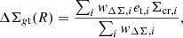
The survey data releases under consideration in this work have covered a total effective sky area (after masking) of ∼1500 deg2 with deep multi-band photometry, see Fig. 1. For full details of each analysis, we refer to the quoted survey papers. Some surveys use multiple pipelines for photometry, shape, and/or photo-z estimates. In Table 1, we report the estimates we used for our work. We motivate our choices below.
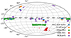 |
Fig. 1. Sky coverage in the equatorial coordinate system of the lensing surveys used in this work. We consider only the tiles with sufficiently reliable shape and photo-z measurements. |
We only use photometry for colour estimates, where differences due to slightly differing transmission filters are sub-dominant for the considered surveys with respect to other effects. Therefore, we do not consider differences in filters or magnitude definitions.
Most of the surveys were designed as dark energy experiments, and were optimised for cosmic shear. These surveys generally quote estimates of area or galaxy density, among others. Here, we are interested in cluster lensing and thus, to ease comparison, we recompute some quantities in a common framework of interest for our specific analysis, see Table 2. Values for these estimates computed in different ways can be found in the survey papers cited here. The estimates of number density or effective area are for the most part consistent, but there are some minor discrepancies.
Weak gravitational lensing properties of the public lensing surveys.
As eligible sources for our analysis, Nsources, we consider galaxies with measured shape, non-null lensing weight, and photo-z. We compute their raw density, nraw, as the mean density in 1000 small random regions of size 2′×2′. The effective survey area Aeff can be estimated as Nsources/nraw.
Most cluster lenses lie at redshift ∼0.3 and sources for cluster lensing are usually recovered from a field of view with proper size of 3–4 Mpc, i.e., half a degree at z ∼ 0.3. We compute the effective density of sources for cluster lensing, neff, as the median of the weighted densities (see Eq. (1) in Heymans et al. 2012) in 1000 random regions of size 30′×30′. We discard the 100 smallest values to mimic selection effects, with clusters less likely to be detected in less populated areas, near borders, or near masked regions.
The raw and effective source densities defined above are defined in a cluster-lensing context. They may differ from the nominal values reported in the reference survey papers and in the following subsections for the different definitions or the different source selections. For our analysis, we exclusively use our homogenised estimates.
2.1. HSC-SSP S16a
The Hyper Suprime-Cam Subaru Strategic Program (HSC-SSP, Miyazaki et al. 2018; Aihara et al. 2018) is an ongoing program to carry out a multi-band imaging survey in five optical bands (g, r, i, z, y) with HSC, an optical wide-field imager with a field-of-view of 1.77deg2 mounted on the prime focus of the 8.2 m Subaru telescope (Miyazaki et al. 2018; Komiyama et al. 2018; Furusawa et al. 2018; Kawanomoto et al. 2018).
The wide survey aims to observe around 1400 deg2 with a depth of i ∼ 26 mag at the 5 σ limit within a 2″ diameter aperture (Aihara et al. 2018). The survey design is optimised for WL studies (Mandelbaum et al. 2018; Hikage et al. 2019; Miyatake et al. 2019; Hamana et al. 2020).
The catalogue of galaxy shape measurements from the first-year data release (S16a) is presented in Mandelbaum et al. (2018). The catalogue covers an area of 136.9 deg2 split into six fields to final depth, with a mean i-band seeing of  . The survey overlaps with the XXL survey (Pierre et al. 2016) in the XXL-North field.
Galaxy shapes were estimated on the co-added i-band images using a moments-based shape measurement method along with the re-Gaussianisation PSF correction method (Hirata & Seljak 2003), which fits a Gaussian profile with elliptical isophotes to the image.
Conservative galaxy selection criteria were implemented to produce the shear catalogue for first-year science, with a magnitude cut of i < 24.5 mag. This results in nominal unweighted and weighted source number densities of 24.6 and 21.8 arcmin−2, respectively (Mandelbaum et al. 2018).
Photo-zs were found to be well determined in the redshift range 0.2 ≲ z ≲ 1.5, with an accuracy of σzphot ∼ 0.05 (1 + zp), and an outlier rate of ∼15% for galaxies down to i = 25 (Tanaka et al. 2018). For the brighter sample of i < 24, performance improves to σzphot ∼ 0.04 (1 + zp) and ∼8% outliers.
We retrieve catalogues from the public archive1. The collaboration provides a variety of estimates for photometric magnitude (Huang et al. 2018) and redshift (Tanaka et al. 2018). Our choices are informed from previous WL cluster analysis of data release S16a (Chiu et al. 2020; Umetsu et al. 2020). We consider photo-zs based on the EPHOR_AB code, which delivers estimates based on PSF-matched aperture photometry (Tanaka et al. 2018). A photo-z risk parameter R(zp) is provided to represent the expected loss for a given choice of zp as the point estimate (Tanaka et al. 2018). For the photometry, we consider the forced cmodel (Huang et al. 2018).
2.2. CFHTLenS
The Canada France Hawaii Telescope Legacy Survey (CFHTLS, Heymans et al. 2012) is a completed photometric survey performed with MegaCam. The final footprint covers four independent fields for a total of 154 deg2 in five optical bands u*, g, r, i, z (Heymans et al. 2012).
The survey was designed for WL analysis, with the deep i-band data taken in sub-arcsecond seeing conditions (Erben et al. 2013). The nominal total unmasked area suitable for cosmic shear analysis covers 125.7 deg2. The nominal raw number density of lensing sources, including all objects with a measured shape, is 17.8 galaxies per arcmin2 (Hildebrandt et al. 2016). The nominal weighted density is 15.1 galaxies per arcmin2 (Hildebrandt et al. 2016).
The CFHTLenS team provided WL data processed with THELI (Erben et al. 2013), and shear measurements obtained with lensfit (Miller et al. 2013), a likelihood based model-fitting method2. Photo-zs were determined with the BPZ algorithm (Benítez 2000), and the ODDS quantifies the prominence of the most likely redshift (Hildebrandt et al. 2012). The photo-zs were measured with accuracy σzphot ∼ 0.04 (1 + z) and a catastrophic outlier rate of about 4% (Hildebrandt et al. 2012; Benjamin et al. 2013).
2.3. KiDS DR4
The Kilo-Degree Survey (KiDS, de Jong et al. 2013) is a European Southern Observatory (ESO) public survey performed with the OmegaCAM wide-field camera mounted at the VLT Survey Telescope (VST). KiDS was designed to observe a total area of 1350 deg2 in the u, g, r, i bands.
The survey area has been observed to full depth, and the analysis is ongoing. The fourth data release (hereafter referred to as KiDS DR4 or KiDS 1000) covered approximately 1000 deg2 in all four survey filters, with complementary aperture-matched Z, Y, J, H, Ks photometry from the partner VIKING survey on the VISTA telescope (Kuijken et al. 2019). The mean limiting magnitudes in the four bands are, respectively, 24.23, 25.12, 25.02, and 23.68 (5 σ in a 2″ aperture).
The survey area is divided into the southern (KiDS-S) and the northern (KiDS-N) fields. KiDS-N contains two additional smaller areas: KiDS-N-W2, which coincides with the G9 patch of the GAMA survey, and KiDS-N-D2, a single pointing on the COSMOS field.
The Astro-WISE information system was used for data processing and catalogue extraction. Shear measurements were done with lensfit, similar to CFHTLenS. Shape measurements were performed on r-band images, as these images exhibit better seeing properties and higher source density (Fenech Conti et al. 2017; Kannawadi et al. 2019). The r-band images were separately reduced with the THELI pipeline for WL science.
We use the gold sample, which includes only galaxies with reliable shape and redshift measurements up to zp = 1.2 (Kuijken et al. 2019; Hildebrandt et al. 2021; Giblin et al. 2021). Cosmological parameter constraints from cosmic shear or galaxy clustering have been presented in such works as Asgari et al. (2021), Heymans et al. (2021), Tröster et al. (2021), Joachimi et al. (2021).
2.4. DES SV1
The Dark Energy Survey (DES) is expected to cover approximately 5000 deg2 in the south Galactic cap region in five optical bands, g, r, i, z, and Y, in a five-year span with the Dark Energy Camera (DECam) (Gatti et al. 2021). The DES Science Verification (SV) survey mimicked the number of visits and total image depth (10 σ limiting magnitude of 24.1 in the i band) planned for the full DES survey (Jarvis et al. 2016).
The largest portion of the SV area, known as SPT-East (SPT-E for short), covers the eastern part of the region observed by the South Pole Telescope (63 deg2). For the present analysis, we consider the SVA1 Gold Catalogue3. The nominal area for the shear catalogues covers 139 deg2.
We consider the shear measurements from the IM3SHAPE shear pipeline on r-band images based on a maximum likelihood fit using a bulge-or-disc galaxy model. For the photo-zs, we consider the BPZ estimates.
Photo-z reliabilities were not provided in the public catalogues. We estimate the confidence in the redshift point estimate zp from the probability density function, in a manner similar to ODDS, as
 (1)
(1)
where we set Δzp = 0.12 (1 + zp), i.e., three times the typical photo-z uncertainty.
2.5. RCSLenS
The RCSLenS is a large public survey performed with MegaCam for WL analyses4 (Hildebrandt et al. 2016). The parent survey, i.e., the Red-sequence Cluster Survey 2 (RCS2, Gilbank et al. 2011) is a sub-arcsecond seeing, multi-band imaging survey in the g, r, i, z bands initially designed to optically detect galaxy clusters.
The survey covers a nominal total unmasked area of 571.7 deg2 down to a magnitude limit of r ∼ 24.3 (for a point source at 7 σ). Photo-zs are available for a nominal unmasked area covering 383.5 deg2, where the nominal raw (weighted) number density of lensing sources is 7.2 (4.9) galaxies per arcmin2. The survey area is divided into 14 patches, the largest being 10 × 10 deg2 and the smallest 6 × 6 deg2.
The shape measurement and data-analysis were performed with tools developed for the CFHTLenS pipeline. A detailed presentation of imaging data, data reduction, masking, multi-colour photometry, photo-zs, shape measurements, tests for systematic errors, and the blinding scheme for objective measurements can be found in Hildebrandt et al. (2016).
3. Cluster samples
We made use of five lens catalogues. Firstly, to compare results from different surveys, assess accuracy, and check for systematic errors, we chose two independent cluster catalogues: (i) the second Planck Catalogue of Sunyaev-Zeldovich Sources (PSZ2, Planck Collaboration XXVII 2016), based on a Sunyaev-Zeldovich (SZ) selection, and (ii) the red-sequence Matched-filter Probabilistic Percolation (redMaPPer) catalogue based on an optical selection on the Sloan Digital Sky Survey (SDSS) DR8 data (Rykoff et al. 2016). These catalogues are extracted from data sets different from the surveys we used for shape measurements. This makes the distribution of lenses uncorrelated with residual systematic effects in galaxy shape measurements (Miyatake et al. 2013; Sereno et al. 2015).
For each lens sample, we used all the clusters that lie in the survey fields without any further selection, and the lensing clusters we considered are an unbiased subsample of the parent catalogue. The main properties of the lensing cluster samples from PSZ2 and redMaPPer per survey are reported in Tables 3 and 4, respectively. Secondly, to study the statistical precision of WL mass measurements, we considered the candidate clusters detected with the Adaptive Matched Identifier of Clustered Objects (AMICO, Bellagamba et al. 2018; Maturi et al. 2019) in the XXL-North field of HSC-SSP. Thirdly, to check for residual systematic effects in the shear calibration, we considered two samples: the clusters detected in HSC-SSP S16a (Oguri et al. 2018) with the Cluster finding algorithm based on Multi-band Identification of Red sequence gAlaxies (CAMIRA; Oguri 2014) and the AMICO clusters in KiDS-DR3 (Lesci et al. 2022). Finally, for comparison with the literature, we considered the Literature Catalogue of weak Lensing Clusters of galaxies (LC2 or LC2; Sereno 2015).
Main properties of the PSZ2 cluster lenses per survey.
Main properties of the redMaPPer cluster lenses per survey.
3.1. Planck PSZ2
PSZ2 is based on the 29 month full-mission data set and contains 1653 candidate clusters (Planck Collaboration XXVII 2016). It is the largest all-sky, SZ selected sample of galaxy clusters produced to date5.
The catalogue includes candidates with S/N above 4.5 located outside the highest-emitting Galactic regions, the Small and Large Magellanic Clouds, and point source masks. 1203 clusters were confirmed with counterparts identified either in external optical or X-ray samples, or by dedicated follow-ups.
Proxy masses (denoted as MSZ or M500cYz) of clusters with known redshift were calibrated with a best fitting scaling relation between M500c and the spherically integrated Compton parameter Y500c (Planck Collaboration XX 2014). The catalogue spans a nominal mass range from MSZ ∼ 0.8 × 10¹⁴ M⊙ to 16 × 1014 M⊙ over the redshift range 0.01 ≲ z ≲ 1.0. The mean redshift is z ∼ 0.25.
Most of the PSZ2 clusters covered by the surveys here considered are at z < 0.6, for which data from Stage-III surveys or precursors can provide reliable masses (Melchior et al. 2015; Sereno et al. 2017; Medezinski et al. 2018). There are two exceptions. PSZ2 G099.86+58.45 at z = 0.63 can be still detected in CFHTLenS with high (S/N)WL (Sereno et al. 2018), whereas PSZ2 G297.97−67.74 at z = 0.87, here covered by DES SV1, is not significantly detected.
3.2. The SDSS redMaPPer catalogue
The redMaPPer algorithm is a red-sequence cluster finder designed for large photometric surveys (Rykoff et al. 2014). Here, we consider the cluster candidates found parsing nearly 10 000 deg2 of contiguous high quality observations of the SDSS DR8 data (Rykoff et al. 2016). The resulting catalogue6 contains 26 111 candidate clusters over the redshift range 0.08 ≲ z ≲ 0.6.
The catalogue provides a richness estimate, λ, defined as the sum of the probabilities of the galaxies found near a cluster to be actual cluster members. The sum extends over all galaxies above a cut-off luminosity (0.2 L*) and below a radial cut that scales with richness (Rykoff et al. 2014).
3.3. AMICO clusters in the XXL-HSC field
AMICO (Bellagamba et al. 2018; Maturi et al. 2019) is an optimal matched filter that takes advantage of the known statistical properties of field galaxies and cluster galaxy members. AMICO can deal with an arbitrary number of quantities describing galaxies. For the AMICO-built catalogues considered here, galaxy angular coordinates, magnitudes, and photo-z were considered, whereas the information concerning the colours was avoided to be independent of the red-sequence (Maturi et al. 2019).
AMICO was selected as one of two cluster selection algorithms for the Euclid mission (Euclid Collaboration 2019a), and has been implemented in the extensively tested Euclid cluster detection pipeline (DET-CL). Here, we consider the runs in the XXL-North field covered by HSC-SSP S18a observations (Euclid Collaboration: Sartoris et al., in prep.).
The XXL-North field has been covered by multi-wavelength observations. HSC-SSP observations over this area from Year 1 have already reached full depth, which makes this an interesting test-case for the Euclid Survey. DET-CL found 3534 candidate clusters with (S/N)det ≥ 3 in the redshift range 0.03 ≤ z ≤ 1.05 with intrinsic richness, λ*, in the range 22.5 ≲ λ* ≲ 591.2 (Euclid Collaboration: Sartoris et al., in prep.). The intrinsic richness is defined as the sum of the probabilities of all galaxies associated with the detection brighter than m* + 1.5 and within the model virial radius.
3.4. CAMIRA clusters in HSC-SSP S16a
Oguri et al. (2018) presented a cluster sample from HSC-SSP S16a, optically selected with CAMIRA (Oguri 2014; Oguri et al. 2018). CAMIRA is a red sequence method that fits each galaxy in the image with a stellar population synthesis model to compute the likelihood to be a red sequence galaxy at a given redshift (Oguri 2014).
Oguri et al. (2018) constructed a catalogue of 1921 clusters from HSC-SSP S16a. The images were sufficiently deep to detect clusters at redshift 0.1 < z < 1.1 with richness  that roughly corresponds to M200m ≳ 1014 h−1 M⊙.
3.5. AMICO clusters in KiDS-DR3
The AMICO algorithm was run in KiDS-DR3 to detect 4934 candidate galaxy clusters with intrinsic richness λ* ≥ 15 and (S/N)det ≥ 3.5 in the redshift range 0.1 ≲ z ≲ 0.8 (Maturi et al. 2019; Lesci et al. 2022).
4. Background source selection
We identify galaxies as background sources for the WL analysis behind the lens at zlens based on their photo-z or colours. As a first step, we select galaxies such that
 (2)
(2)
where zp is the redshift point-estimate and Δzlens is a threshold above the cluster redshift to lower the contamination.
On top of this criterion, we require that the sources pass more restrictive cuts in either photo-z or colour properties, which we discuss below.
4.1. Photometric redshifts
A population of background galaxies can be selected with criteria based on the photo-zs (Sereno et al. 2017):
 (3)
(3)
 (4)
(4)
 (5)
(5)
 (6)
(6)
where the parameter zp, confidence is a measure of the confidence we have in the point estimate of the redshift; zp, 2.3% is the lower bound of the region including the 95.4% of the probability density distribution; Δzlens is a conservative threshold to better select background galaxies, see Eq. (2); zp, range, min and zp, range, max are the boundaries of the redshift range wherein photo-z estimates are thought to be reliable.
The redshift range can be chosen based on the survey depth or such that the photometric bands straddle the 4000 Å break. Employed parameters and cuts for each survey are listed in Table 5.
Parameters for the photo-z background selection.
4.2. Colour-colour
Selection of background galaxies in colour-colour (CC) space can be highly effective and provide very complete and pure samples (Euclid Collaboration 2024). Here, we adopt the cuts in the g − i vs. r − z CC space proposed in Medezinski et al. (2018), which spans the optical range observed by the considered surveys. Different populations of galaxies are efficiently separated in this space and the level of contamination is consistent with zero within a 0.5% uncertainty. The cuts are detailed in Medezinski et al. (2018, Appendix A).
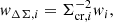
The distribution of sources per survey that would be considered as background for a lens plane at zlens = 0.4 is shown in Fig. 2.
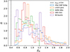 |
Fig. 2. Normalised distribution of the photo-zs up to zp = 2 for selected sources behind a lens plane at zlens = 0.4. The sources are selected either with robust cuts in photo-z or in colour-colour space. |
5. WL signal
The lensing signal is recovered from the measured shapes of the background galaxies.
5.1. Signal definition
As the main observable, we considered the tangential reduced excess surface density ΔΣgt, which can be expressed in terms of the surface density, Σ, and of the tangential excess surface density ΔΣt. For an axially symmetric lens and a single source plane,
 (7)
(7)
where R is the transverse proper distance from the assumed lens centre, and Σcr is the critical density for lensing,
 (8)
(8)
where c is the speed of light in vacuum, G is the gravitational constant, and Dl, Ds, and Dls are the angular diameter distances to the lens, to the source, and from the lens to the source, respectively.
The tangential reduced excess surface density can be rewritten in terms of the reduced tangential shear, gt = γt/(1 − κ), where γt is the tangential shear, and κ ≡ Σ/Σcr is the convergence, as
 (9)
(9)
For a population of sources distributed in redshift, the source averaged excess surface mass density can be approximated as (Umetsu 2020)
 (10)
(10)
The equations here presented hold for non-axially symmetric lenses too if we consider azimuthally averaged quantities.
5.2. Signal measurement
If ⟨eα⟩, i.e., the ensemble average of the shape measurements eα, where α = 1, 2 denotes the shear component in the Cartesian plane, is an unbiased estimator for the reduced shear (Schramm & Kayser 1995; Seitz & Schneider 1997; Bernstein & Jarvis 2002; Miller et al. 2013),
 (11)
(11)
the reduced excess surface density ΔΣgt in circular annuli can be estimated from the sum over the sources inside each annulus as
 (12)
(12)
where
 (13)
(13)
and et, i is the tangential component of the ellipticity of the i-th source galaxy, wi is the weight assigned to the source ellipticity, and Σcr, i is the critical density for the i-th source. The sum runs over the galaxies included in the annulus centred at R.
In the following, we use the notation ⟨…⟩ΔΣ for a weighted average, where wΔΣ, i are the weights. With this notation, Eq. (12) can be rewritten as
 (14)
(14)
Some shape measurements, such as the ellipticity |ϵ|=(1 − q)/(1 + q), where q is the image axial ratio, from lensfit or IM3SHAPE, fulfil Eq. (11), i.e., ϵi = ei. For other shape estimates, e.g., the distortion |δ|=(1 − q2)/(1 + q2) measured by the re-Gauss algorithm (Mandelbaum et al. 2008), GALSIM (Rowe et al. 2015), or KSB-like algorithms (Kaiser et al. 1995), one must account for the responsivity ℛ:
 (15)
(15)
The responsivity can be calculated based on the inverse variance weights and the per-object estimates of the RMS distortion δRMS, i as (Mandelbaum et al. 2018)
 (16)
(16)
For our analysis, a responsivity calculation is needed to process the HSC-SSP data.
The source averaged reduced excess surface mass density can be approximated as in Eq. (10) with the ⟨…⟩ΔΣ average,
 (17)
(17)
We compute distances to the sources and critical surface densities in Eq. (8) based on the photo-z point-estimator. Methods exploiting the per-source photo-z probability density function (see, e.g., Sheldon et al. 2004) or the ensemble source redshift distribution (see, e.g., Hildebrandt et al. 2020) have been advocated, too. Some methods need inherently unbiased and accurate representations of the redshift probability distribution and of systematic uncertainties, which might be difficult to achieve (Tanaka et al. 2018; Hildebrandt et al. 2020). However, the level of systematic errors introduced by either the point-estimator or the probability density function for quality photo-zs and robust selections is usually sub-dominant for Stage-III surveys (see, e.g., Bellagamba et al. 2019).
The present version of the Euclid data processing pipeline for cluster weak lensing relies on photo-z point-estimators. Pros and cons of different approaches are discussed in Leauthaud et al. (2022) and references therein.
We measure the average reduced excess surface density ΔΣgt in eight radial circular annuli equally separated in logarithmic space spanning the range between Rmin = 0.3 h−1 Mpc (∼0.43 Mpc) and Rmin = 3.0 h−1 Mpc ( ∼ 4.3 Mpc) from the cluster centre.
5.3. Calibration
The raw shape components of the source galaxies, eraw, 1 and eraw, 2, can exhibit a bias that can be parameterised by a multiplicative (m) and an additive (c) component,
 (18)
(18)
which must be calibrated. If needed, we correct each galaxy for the additive bias, whereas the multiplicative bias m is averaged in each annulus (Heymans et al. 2012; Miller et al. 2013; Viola et al. 2015),
 (19)
(19)
5.4. Signal-to-noise
The S/N of the WL cluster can be defined in terms of the weighted excess surface density ΔΣgt in the relevant radial range Rmin < R < Rmax (Sereno et al. 2017),
 (20)
(20)
where the noise δt includes statistical uncertainties, and cosmic noise (if relevant) added in quadrature.
For our analysis, we consider (S/N)WL between Rmin = 0.3 h−1 Mpc and Rmin = 3.0 h−1 Mpc from the cluster centre.
6. Mass inference
Cluster masses can be determined fitting the shear profiles in a fixed cosmological model. The general framework is detailed in Sereno et al. (2017) and Umetsu (2020) for example (and references therein). Here, we only discuss the specific setting adopted for the present analysis.
6.1. Halo model
We model the lens either with a simple Navarro, Frenk, White (NFW) profile (Navarro et al. 1996), characterised by mass, M200c, and concentration, c200c, or with a composite model consisting of a Baltz, Marshall, Oguri (BMO) profile (Baltz et al. 2009), e.g., a truncated NFW profile, parameterised by mass, concentration, and truncation radius, rt, plus a two-halo term for the correlated matter characterised by the environment bias, be (Sereno et al. 2018). We refer to the second model as BMO+2-halo. The NFW model can be seen as a specific form of the BMO model, with be = 0 and rt → ∞.
For the fitting parameters, we consider the logarithm (base 10) of mass and concentration, p = (logM200c, logc200c). Here, logM200c is short for log10[M200c/(1014 M⊙)].
The contribution from the uncorrelated large-scale structure (LSS) is treated as a source of noise (Sereno et al. 2017). The cross-correlation between two angular bins Δθi and Δθj can be written as (Schneider et al. 1998; Hoekstra 2003)
 (21)
(21)
where Pk(l) is the effective projected power spectrum of lensing. We compute the linear matter power spectrum with a semi-analytical fitting function (Eisenstein & Hu 1998), which is adequate for the precision needed in our analysis. The effects of non-linear evolution are accounted for with the revised halofit model (Takahashi et al. 2012). The function g is the filter. In an angular bin θ1 < Δθ < θ2,
![Mathematical equation: $$ \begin{aligned} g=\frac{1}{\pi (\theta _1^2 -\theta _2^2)l} \left[ \frac{2}{l} \left( J_0(l \theta _2) -J_0(l \theta _1) \right) +\theta _2 J_1(l \theta _2) -\theta _1 J_1(l \theta _1) \right]. \end{aligned} $$](/articles/aa/full_html/2024/09/aa48680-23/aa48680-23-eq24.gif) (22)
(22)
6.2. Inference
The lens parameters are measured with a Bayesian analysis, where the posterior probability density function of the parameters, p, given the data, {⟨ΔΣgt⟩}, can be written as
 (23)
(23)
where p is a vector including the model parameters, ℒ is the likelihood, and pprior is the prior.
The likelihood is ℒ∝exp(−χ12/2), where χ2 is written as
![Mathematical equation: $$ \begin{aligned} \chi ^2 = \sum _{i,j} \left[ \langle \Delta \Sigma _{g\mathrm{t}}\rangle _i - \Delta \Sigma _{g\mathrm{t}} (R_i | \mathbf p ) \right]^\mathrm{t} \mathsf{C }_{ij}^{-1} \left[ \langle \Delta \Sigma _{g\mathrm{t}}\rangle _ij - \Delta \Sigma _{g\mathrm{t}} (R_j | \mathbf p ) \right]; \end{aligned} $$](/articles/aa/full_html/2024/09/aa48680-23/aa48680-23-eq26.gif) (24)
(24)
the sum extends over the radial annuli; ΔΣgt(Ri|p) is the halo model computed at the lensing weighted radius Ri of the i-th bin (Sereno et al. 2017); and ⟨ΔΣgt⟩i is the measured reduced excess surface density in the i-th bin.
Shape noise, δΔΣStat, and lensing from LSS, ΔΣLSS, are treated as uncertainties. The total uncertainty covariance matrix is
 (25)
(25)
where Cstat accounts for the uncorrelated statistical uncertainties in the measured shear, and  , where Δθi is the i-th annular bin, is due to LSS (Sereno et al. 2017; Umetsu et al. 2020).
The main source of noise is the intrinsic ellipticity dispersion σeα. For Euclid, a reference value of σeα = 0.26 was estimated from a sample of galaxies observed with the Hubble Space Telescope and with similar photometric properties to those expected from Euclid (Schrabback et al. 2018a; Euclid Collaboration 2019b, 2023a).
Here, we do not consider correlated shape noise due to intrinsic alignment of sources, which can be neglected for Stage-III analyses of cluster lensing (McClintock et al. 2019; Umetsu et al. 2020) but it might play a role for Euclid and Stage-IV analyses of clusters and their outskirts (Sereno et al. 2018).
6.3. Priors
We consider non-informative, uniform priors in log-space, as suitable for positive quantities, with −1 < logM200c < 2 and 0 < logc200c < 1.
The truncation radius and environment bias are fixed. For the BMO+2-halo model, the truncation radius is set to rt = 3 r200c, and the environment bias be is fixed with a Dirac delta prior as a function of the peak height ν, be = bh[ν(M200c, z)] (Tinker et al. 2010).
7. Consistency tests
To detect the degree of any potential discrepancy between independent results, we utilise two metrics. Let Qa and Qb be two sets of parameters, with total uncertainty expressed through the covariance matrix CQa, b. The χ2 can be defined as
 (26)
(26)
For uncorrelated data, the covariance matrix is diagonal with the diagonal terms given by the sum of the squared uncertainties,
 (27)
(27)
where δQa and δQb are the uncertainties on Qa and Qb, respectively.
Given a χ2 distribution with Nd.o.f. degrees of freedom, we can calculate the probability to exceed a given value, p(χ2 > χa, b2; Nd.o.f.), and use this probability as a metric for comparison.
When we compare a scalar quantity Qi, we consider
 (28)
(28)
where 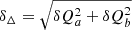 .
.
As a second metric, we consider a function based only on the point-estimates. We compute the CBI of the differences,
 (29)
(29)
and the associated SBI,
 (30)
(30)
The estimator ΔSBI quantifies the dispersion of the results. The uncertainty on ΔCBI, δΔCBI, can be computed by bootstrapping the sample and computing the SBI of the summary CBI statistics. Any value of ΔCBI in excess of the statistical uncertainty can point to systematic effects or statistical uncertainties biased low. We report the Δ metric as ΔCBI(±δΔCBI)±ΔSBI.
The main observable quantities we considered for comparison are the radial profiles of the reduced excess surface density, Qa = {⟨ΔΣgt, survey(Ri)⟩}, with Nd.o.f. given by the number of bins, and the lens masses of a sample, Qa = {logM200c, survey, i}, with Nd.o.f. given by the number of clusters. When we compared the total signal ΔΣgt(Rmin < R < Rmax), we used Δχ as the main metric.
8. WL signal accuracy
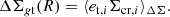
To assess the accuracy to which the WL signal can be measured, we compare the average radial profiles of the reduced excess surface density of the lenses, ΔΣgt, survey(Ri), from different surveys, see Fig. 3. We measure the signal in eight radial bins (Nd.o.f. = Nbin = 8).
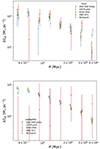 |
Fig. 3. Average reduced excess surface density profiles of clusters detected in public surveys as a function of R, the transverse proper distance from the lens centre, coded by colours as in the legend. Top: PSZ2 clusters. Bottom: Sample of redMaPPer. |
In our approach, statistically significant differences between results from different surveys are seen as indications of systematic errors. An analysis with underestimated statistical uncertainties is then conservative as it can inflate differences. When comparing the WL profiles, we only account for the total shape noise including the intrinsic shape dispersion per component and the per-component shape measurement error. We do not account for noise from either correlated or uncorrelated LSS.
Different surveys share lenses and source galaxies in overlapping regions, and intrinsic ellipticity and shape noise are correlated to some degree. This is difficult to quantify at the catalogue level. Ellipticity values measured with a different resolution, in a different galaxy radial range, with different effective radial weight functions, or in different bands might vary, as the spatial distribution of the light emission may not be identical (Schrabback et al. 2018b). We very conservatively quantify the correlation assuming that lensing signal of shared clusters is fully correlated.
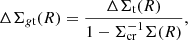
We measured the reduced excess surface density, which unlike the excess surface density, brings some residual dependence on source and lens redshift, mostly in the inner regions (see Eq. (17) in Umetsu 2020). Notwithstanding our simplifying and conservative assumptions, the agreement between the profiles measured in different surveys is significant both for Planck, see Table 6, and redMaPPer clusters, see Table 7.
Comparison of the average reduced excess surface density profiles of the Planck clusters detected in different surveys.
Comparison of the average reduced excess surface density profiles of the redMaPPer clusters detected in different surveys.
Discrepancies between surveys are smaller than statistical uncertainties. This implies that shear can be accurately calibrated and known systematic effects are properly accounted for. For Stage-III surveys and precursors, unknown or residual systematic effects either play a negligible role or very fortuitously counter-balance each other among different surveys and data sets.
The validity of the test relies on the assumption that the cluster subsamples, which are selected from different survey footprints, are homogeneous. This assumption may be invalid if the properties of the parent samples vary spatially (Leauthaud et al. 2022). Even if the samples are spatially homogeneous, we are sampling a small number of clusters per survey, which might not fairly sample the full parent population of dark matter haloes. On the other hand, this choice of the lens samples per survey limits the correlation of sources. Some concerns on the lens samples can be solved by analysing lenses that are covered by more than one survey. In fact, for the four Planck clusters covered by a pair of surveys, we found statistical agreement, see App. B.
In App. C, we perform a cross-check between shear calibrations by comparing the WL profile of clusters extracted by matched source catalogues from different surveys to show how residual effects for Stage-III surveys and precursors are negligible with respect to the statistical uncertainties.
9. Mass accuracy
In this section, we report results on the accuracy we can reach in mass measurements of cluster masses from survey data. The section serves a dual purpose. On one hand, we cross-validate Stage-III surveys by comparing results obtained from a uniform, consistent analysis. Agreement can indicate that the different data sets are compatible and that systematic errors in each survey are corrected to the required levels.
On the other hand, fitting procedures here employed for WL profiles and WL mass estimates can be validated by comparison with literature results.
As a reference fitting model, we considered the BMO+2-halo model. For the uncertainty budget, we considered contributions from both shape noise and LSS.
We first look for potential systematic effects by comparing results exploiting different analysis assumptions, see Sects. 9.1 and 9.2. Then we compare results from different surveys, see Sect. 9.3, or with estimates from the literature, see Sect. 9.4.
9.1. Mass point-estimators
In the regime of low signal-to-noise, the inferred probability distribution for the mass can be very skewed. The peak may not be prominent and the distribution can show a strong tail to very low values. In the case of negative (S/N)WL, the distribution could be better summarised by an upper limit rather than an estimate of the central location.
In Table 8, we compare different mass point-estimates of the PSZ2 clusters. We consider the maximum likelihood (ML) value as well as the biweight location CBI, the median, and the mean of the posterior probability distribution. Point-estimates can significantly differ. As expected for a distribution sampled with a long chain, estimates of the median and the CBI are in very good agreement. The agreement with the mean is also good, though with a larger dispersion. On the other hand, ML estimates are usually larger than CBI or mean estimates, even when considering the large dispersion.
Comparison of mass point-estimators of the PSZ2 clusters.
Any mass point-estimate (and a related uncertainty) might fail in summarising the mass posterior, and the full probability distribution should be considered. For example, using the mass location and scale in analyses that implicitly assume a Gaussian distribution can significantly bias the results if the mass probability distribution is not Gaussian. The use of the full probability distribution is recommended in the low (S/N)WL regime.
In the following, when comparing our results with literature values, we try to use the most appropriate estimator, i.e., the estimator that most resembles the properties of the comparison sample.
9.2. Halo model
A proper modelling of the lens is crucial for an unbiased mass determination (Oguri & Hamana 2011). We estimate the effects of halo modelling in Stage-III surveys and precursors by comparing mass point-estimates of the PSZ2 clusters derived by modelling the lens either with BMO+2-halo or NFW profiles. Results are consistent with ΔCBI ± ΔSBI = −0.03 ± 0.02, −0.05 ± 0.24, −0.05 ± 0.24, and −0.05 ± 0.22 for the ML, CBI, median, and mean, respectively.
Halo modelling can play a larger role when fitting the very inner regions, where the inner slope has to be properly accounted for (Sereno et al. 2016), or the outer regions where the matter distribution transits to the infalling region (Diemer & Kravtsov 2014), or with the better data quality expected for Stage-IV surveys. At the level of the present analysis, where we consider Stage-III surveys and precursors and exclude the inner and outer radial regions from the fitting, the role is minor. We only consider the BMO+2-halo model in the following.
9.3. Clusters covered by multiple surveys
A number of redMaPPer clusters are covered by multiple surveys. For these clusters, we can directly compare the mass estimates.
Any correlation between mass estimates, which is not properly accounted for, can underestimate the statistical significance of mass differences. Three sources of correlation are the galaxies shared by different surveys in overlapping regions, the noise from uncorrelated matter, and the common fitting scheme.
Firstly, different surveys share the same source galaxies in overlapping regions, and intrinsic ellipticity and shape noise are correlated to some degree. As discussed in Sect. 8, this can be quantified with working assumptions. When cross-comparing two surveys, we can assume that the deeper survey detects and measures shear for all the galaxies detected and measured by the shallower survey in the overlapping region. For example, for an hypothetical lens at zlens = 0.38, as is typical for redMaPPer clusters, see Table 4, we can assume that all background sources detected in KiDS DR4 are also selected in HSC-SSP S16a. This would account for ∼30% of the full background source sample in HSC-SSP S16a. If we neglect differences in intrinsic ellipticity due to different bands or spatial extents, this would entail a correlation of ∼0.5 in the measured shear.
Secondly, mass measurements of the same cluster from different surveys experience the same noise from uncorrelated matter. Even though the LSS noise is mostly negligible with respect to the shape noise for Stage-III surveys or precursors, it can still entail some correlation in the shape measurements. For a KiDS-like survey, the LSS noise is ∼50% of the shape noise for a lens at zlens = 0.38 in the radial range we considered for fitting, which would entail a correlation of ∼0.2. When correlated shape and LSS noise are considered together, the correlation would be ∼0.7 when comparing mass estimates based on either KiDS DR4 or HSC-SSP S16a.
Finally, if we consider that the use of the same pipeline for mass measurements can further correlate the estimates, we can conservatively consider a total correlation of ∼0.8. We will use this estimate of the correlation for our comparison.
Results for the redMaPPer clusters are summarised in Table 9, where we report results for the mass biweight point-estimator, and we find agreement between different surveys. This can be seen as a consequence of the agreement between the shear profiles, discussed in Sect. 8.
Comparison of WL masses of redMaPPer clusters covered by multiple surveys.
9.4. Comparison with the WL mass from literature
To assess the robustness of WL mass estimates, we compare masses of PSZ2 or redMaPPer clusters obtained using COMB-CL on survey data with literature values. We first consider the LC2 meta-catalogues (Sereno 2015) in Sect. 9.4.1, and then two smaller, but homogeneous and statistically complete samples, PSZ2LenS (Sereno et al. 2017) in Sects. 9.4.2, and HSC-XXL (Umetsu et al. 2020) in 9.4.3. LC2 is mostly based on follow-up, targeted observations independent of the survey data we consider here. By comparison, we can test the robustness of the mass estimates to data and analysis systematics. On the other hand, PSZ2LenS or HSC-XXL have to a large extent exploited the same survey data considered here. By comparing with their results, we can gain insight into the robustness to analysis choices.
The degree of correlation of our mass uncertainties with literature results from a meta-catalogue is difficult to quantity but it is expected to be smaller than for a mass comparison between results exploiting overlapping survey data and a uniform pipeline. Literature results are usually based on targeted observations that cover a smaller radial extent than a survey. This often leads to a small fraction of common source galaxies. Furthermore, methods used to select background galaxies or to measure galaxy ellipticity follow very heterogeneous pipelines, which can further lower the degree of correlation due a shared subsample of source galaxies.
On the other hand, noise from correlated or uncorrelated matter can make the measurements correlated. Following Sect. 9.3, we can estimate a correlation of 0.2 due to LSS noise, and we use this estimate when comparing our masses with masses from LC2.
9.4.1. LC2
As a first comparison sample, we consider LC2, a large compilation of WL masses retrieved from the literature and periodically updated (Sereno 2015)7. The latest compilation (v3.9) lists 1501 clusters and groups (806 unique) with measured redshift and WL mass from 119 bibliographic sources. The catalogues report coordinates, redshift, WL masses to over-densities of 2500, 500, 200, and to the virial radius, and spherical WL masses within 0.5, 1.0, and 1.5 Mpc in a reference cosmological model.
We identify counterparts in the LC2 catalogue by matching with clusters from the lens samples whose redshifts differ for less than Δz = 0.05 (1 + zlens) and whose projected distance in the sky does not exceed 10′. We found 47 (44 unique) matches for PSZ2 and 158 (119 unique) matches for redMaPPer. We consider a threshold in arcmin since the Planck positional accuracy is driven by the angular PSF. Matching results do not significantly change considering thresholds in proper lengths (e.g. a projected distance in the sky that does not exceed 1 Mpc).
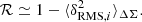
The ML estimator is often considered for mass point estimates. To ease comparison with literature values, we adopted this estimator. We found no evidence of disagreement (see Fig. 4 and Tables 10 and 11). For the quantitative comparison, we excluded 11 clusters with low (S/N)WL whose mass estimate collapses on the lower bound of the prior range and for which the median or mean estimator would have been more appropriate. Results do not significantly depend on their exclusion.
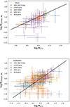 |
Fig. 4. Maximum likelihood estimates of M200c of clusters as obtained with the COMB-CL analysis of public surveys (colour-coded according to the legend) versus literature masses from the LC2 catalogue. Top: PSZ2 clusters. Bottom: Sample from redMaPPer. |
Comparison of Planck cluster masses from the COMB-CL analysis of public surveys with literature values.
Comparison of redMaPPer cluster masses from the COMB-CL analysis of public surveys with literature values.
Some of the results collected in the LC2 catalogues were based on survey data. For example, Sereno et al. (2017) and Medezinski et al. (2018) studied PSZ2 clusters covered by CFHTLenS/RCSLenS or HSC-SSP 16A, respectively. This makes the results correlated to some degree. However, the LC2 sample is heterogeneous and mostly based on independent, targeted follow-up observations.
9.4.2. Comparison with PSZ2LenS
Sereno et al. (2017) studied the PSZ2LenS sample, i.e., the PSZ2 clusters covered by CFHTLenS and RCSLenS. Most of the LC2 matches with PSZ2 are from their analysis. Considering only the matches with PSZ2LenS, we lose some statistical power with respect to the full LC2 vs. PSZ2 comparison, but we can exploit a better defined, statistically complete, and homogeneous comparison sample. We find consistent results, see Table 10, notwithstanding some notable differences with respect to Sereno et al. (2017).
Here, we are interested in survey results, and we consider lens properties as reported in the cluster catalogues without further elaboration. Sereno et al. (2017) re-examined the Planck candidates, re-centred them to the brightest cluster galaxy (BCG), and re-examined the cluster redshifts reported in the catalogue. However, miscentring effects were found to be small (Sereno et al. 2017).
To perform a multi-survey analysis, we select background galaxies with a colour cut in r − z and g − i. This is very convenient for deep surveys such as HSC-SSP. For a much shallower survey such as RCSLenS, a colour selection in g − r and r − i, as done in Sereno et al. (2017), may be more convenient to collect a larger number of low redshift sources and boost the WL signal.
Finally, Sereno et al. (2017) considered a uniform prior for the mass, which may favour larger masses with respect to our prior, which is flat in log-space. Notwithstanding the differences in analyses, agreement is good (see Table 10).
9.4.3. HSC-XXL
Umetsu et al. (2020) performed a WL analysis of 136 spectroscopically confirmed X-ray detected galaxy groups and clusters selected from the XMM-XXL survey (Pierre et al. 2016; Adami et al. 2018) in the 25 deg2 XXL-North region and covered by the HSC-SSP first-year data. The overlap with the redMaPPer sample is significant, see Table 11, and we can perform a comparison with a homogeneous analysis from the literature. WL masses reported in Umetsu et al. (2020) were rescaled to our reference cosmological model following Sereno (2015).
Umetsu et al. (2020) exploited the same HSC-SSP data release used in the present analysis, and we consider the same photo-z estimates, but some noteworthy differences still remain. Umetsu et al. (2020) considered the radial range within a comoving cluster-centric radius of 3.0 h−1 Mpc, whereas we consider proper lengths. They did not perform background selection in the colour-colour space. They adopted a NFW model with log-uniform priors. Umetsu et al. (2020) centred clusters in the X-ray peak, which can differ from the redMaPPer centre. Notwithstanding the differences, our analyses share the WL data set (for HSC-SSP-16a) and some major assumptions. Umetsu et al. (2020) considered the biweight location as the mass point-estimate and to be consistent, only for the sake of this comparison, we consider the same estimator. Results are in good agreement, see Table 11.
9.5. Discussion
The agreement between mass measurements, estimated with a uniform fitting scheme, of the same clusters covered by multiple surveys further supports the agreement between the different data sets from Stage-III surveys and precursors, and the agreement of the inferred shear profiles. The agreement between shear profiles is a prerequisite for consistent mass measurements. Therefore, if we check for mass agreement, we also check that this prerequisite is met.
The agreement of our mass measurements with literature results derived both from large, heterogeneous compilations, or smaller but homogeneous analyses, demonstrates that the fitting procedures for WL mass estimates are robust at the level required by Stage-III surveys.
We do not correct for miscentring or residual cluster member contamination, which reduce the signal and can make the derived masses systematically lower than what was found in dedicated analyses from the literature. On the other hand, correlation in shear estimates can lower the level of disagreement. However, our comparison showed that different treatments of the halo model, line-of-sight projections, correlated matter or LSS, triaxiality, contamination and membership dilution, miscentring, or priors still yield WL mass estimates consistent within the statistical uncertainty for Stage-III surveys and precursors.
Our analysis suggests that residual or unknown systematic effects are sub-dominant with respect to known effects for Stage-III surveys and precursors. Comparison of WL masses of redMaPPer clusters covered by multiple surveys, see Table 9, shows a mass accuracy of ∼1 ± 2%. This result is mostly driven by the cross-comparison of the HSC-SSP S16a and the KiDS DR4 surveys, with 343 redMaPPer clusters in the overlapping fields, but cross-checks are also consistent for other surveys.
The cross-comparison under a unified scheme can show biases at the catalogue level, such as biases due to the calibration of either shear or photo-z measurements, but might be insensitive to modelling assumptions concerning miscentring or background selection, for example. Dependence on the mass point estimator, see Sect. 9.1 and Table 8, or halo model, see Sect. 9.2, is subcritical. The total level of systematics can be assessed by comparison with literature values. Considering the 130 (with duplicates) redMaPPer clusters with known WL masses covered by the surveys under considerations, see Table 11, we infer an accuracy of ∼1 ± 8%. This estimate could be inflated due to the heterogeneity of the comparison sample.
10. Mass precision
The Euclid Survey will cover about 15 000 deg2 of the extra-galactic sky (Euclid Collaboration 2022b) and Euclid will deliver an unprecedented number of clusters with high (S/N)WL. In this section, we want to discuss the statistical precision of WL mass measurements in Stage-III surveys and the expectations for Euclid. We first discuss the status quo for mass measurements in ongoing or completed surveys. Then, we make a forecast for Euclid with a semi-analytical approach. Finally, we extrapolate the results from Stage-III surveys and precursors to make a data-driven forecast for Euclid.
10.1. Intermediate and massive clusters
WL measurements of individual clusters are very challenging. For the more massive and well observed clusters, only a mass precision of the order of about 10% can be reached (Applegate et al. 2014; Umetsu et al. 2016). In Fig. 5, we plot the distribution of the (S/N)WL of the PSZ2 and redMaPPer clusters per survey. Some survey specifics are listed in Tables 3 and 4. Cumulative statistics for (S/N)WL are reported in Tables 12 and 13.
 |
Fig. 5. Binned distribution of (S/N)WL of clusters that lie in public surveys, coded by colour as in the legend. Top: PSZ2 clusters. Bottom: Sample from redMaPPer-SDSS. |
Number of PSZ2 clusters per survey with (S/N)WL larger than a given threshold.
Number of redMaPPer clusters per survey with (S/N)WL larger than a given threshold.
The very massive end of the halo mass function is covered by the redMaPPer sample (up to z ∼ 0.6) and the PSZ2 sample (up to z ∼ 1). However, (S/N)WL exceeds 3 only for a few lenses. We find 50 redMaPPer lenses with (S/N)WL ≥ 3 from a total multi-survey area of ∼1500 deg2 covered with a not homogeneous depth.
10.2. Small groups
In a photometric survey, clusters can be detected from the same data set used for shape measurements. In Figs. 6 and 7, we consider the distribution of the AMICO clusters detected in XXL-North exploiting the HSC-SSP data, see Sect. 3.3. For 1474 clusters (∼42% of the total sample), (S/N)WL is negative. Based on WL data only, we could not detect them. Mass can be significantly constrained only for a few very rich clusters.
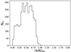 |
Fig. 6. Binned distribution of (S/N)WL of the candidate clusters detected by AMICO in the XXL-North field covered by HSC-SSP S16a. |
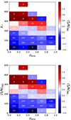 |
Fig. 7. (S/N)WL of the clusters and groups detected by AMICO in the XXL-North field of HSC-SSP. Top: (S/N)WL as a function of redshift and richness. The (S/N)WL is computed as the median value for the candidate groups in the bin, and (S/N)WL is colour-coded as shown in the right bar. The number of candidates is superimposed in each bin. Bottom: Same as in the top panel for (S/N)WL as a function of redshift and (S/N)det. In other words, this panel shows the S/N of the optical detection of the algorithm. |
The AMICO-defined S/N for optical detection, (S/N)det, is nearly one order of magnitude larger than the corresponding (S/N)WL. (S/N)WL exceeds 2 (3) only for 28 (5) out of 3541 detections with (S/N)det ≥ 3.
10.3. Semi-analytical forecasting
The expected number of Euclid clusters with a well measured WL mass can be estimated using a semi-analytical approach. We first estimate the expected (S/N)WL of a lens at a given mass and redshift. Subsequently, we estimate the limiting mass at a given redshift such that the mean (S/N)WL is above a given threshold. We finally estimate the number of clusters above this threshold mass.
As in Sect. 5, we consider the signal collected in the radial range between 0.3 and 3.0 h−1 Mpc from the cluster centre. We model the cluster as a NFW halo whose concentration follows the mass-concentration relation from Diemer & Joyce (2019).
For noise, we consider either shape noise and LSS noise or shape noise only. Galaxy shape noise is mainly due to intrinsic ellipticity, which we model as being Gaussian distributed with σint = 0.26, as measured for a sample of galaxies observed by the Hubble Space Telescope with similar photometric properties to those expected from Euclid (Schrabback et al. 2018a; Euclid Collaboration 2023a).
Given the resolution and depth of Euclid, we anticipate that the survey can measure galaxy shapes with a density of about 30 galaxies per arcmin2 (Laureijs et al. 2011). To model the source distribution, we consider the Euclid-like distribution of sources approximated from the COSMOS2015 photometric redshift catalogs (Laigle et al. 2016) by Martinet et al. (2021), and modelled as proposed in Fu et al. (2008), with parameters from Euclid Collaboration (2023a).
For the source selection, we consider one third of the Euclid sky to be masked. Subsamples of sources with high completeness can be extracted in Euclid with a robust selection at the sub-percent contamination level (Euclid Collaboration 2024). This can be approximated by selecting 80% of the galaxies with z > zlens + 0.1, see Eq. (2).
We can then compute the mass threshold for a halo to have mean (S/N)WL larger than a given threshold value defined as a function of redshift. The threshold mass is shown in Fig. 8. Shape noise or noise contribution from LSS to the shear smoothly increase with the lens redshift, as well as the reduced shear, but the different growth rates at low redshift cause the upturn. For shape noise only, the mass threshold for (S/N)WL > 3 can be approximated as
 (31)
(31)
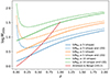 |
Fig. 8. Expected mass thresholds for WL mass precision with Euclid as a function of redshift. For each redshift, we plot the minimum mass for which the mean (S/N)WL is expected to exceed a threshold in the reference cosmology. For comparison, we also show the result from Andreon & Bergé (2012) for a different (S/N)WL definition. |
Finally, we compute how many haloes exceed the mass threshold in a ΛCDM universe. We model the halo mass function as proposed in Tinker et al. (2008). The mass threshold in Eq. (31) is much larger than the mass limit for optical detection and we expect the cluster sample to be complete in this mass range. We consider the redshift range 0.1 < z < 2.0 and we assume that all clusters with (S/N)WL ≥ 3 in this redshift range can be optically detected.
The total number of clusters with mean (S/N)WL larger than a threshold can be found by integration of the halo mass function.
Considering shape noise only, we find ∼14 800, ∼2400, ∼90 clusters with (S/N)WL ≥ 3, 5, 10, respectively, in the redshift range 0.1 < z < 2.0. The redshift distribution of clusters is shown in Fig. 9. The mean lens redshift is ∼0.37. We expect ∼1600 (100), 250 (8), or 20 (0) clusters at z > 0.6, 0.8, or 1.0, respectively, with (S/N)WL ≥ 3 (5).
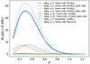 |
Fig. 9. Expected number of clusters (in small redshift bins of Δz = 0.001) with (S/N)WL in excess of a given threshold. We show results for different (S/N)WL thresholds (three, five, ten); halo mass function modelling, either from Tinker et al. (2008) or Despali et al. (2016); and cosmological models (the reference one or Planck18). |
The main source of uncertainty in this forecasting is due to the cosmological model. We estimated an uncertainty of ±3000 by comparing the expected number of clusters with mean (S/N)WL ≥ 3 with the results obtained using a halo mass function with cosmological parameters derived from the final Planck data release of Cosmic Microwave Background anisotropies (Planck Collaboration VI 2020). Uncertainties due to the modelling of the halo mass function (±600) were estimated comparing to results based on the halo mass function proposed by Despali et al. (2016). These uncertainties can be added to give a final estimate of 15 000 ± 4000 expected clusters with (S/N)WL ≥ 3.
Andreon & Bergé (2012) performed a forecast for the expected number of WL selected clusters. Notwithstanding the substantial differences compared to our analysis (e.g. different definitions of (S/N)WL), different treatments of masks, photometric redshift uncertainty, member and foreground contamination, and LSS noise, we find that the total expected number of clusters agrees with their estimate.
Noise from LSS will be one of the main sources of uncertainty for WL mass calibration in Stage-IV surveys (Köhlinger et al. 2015). If we consider both shape and LSS noise, the number of clusters with a large (S/N)WL is significantly reduced. We find ∼3000, ∼260, ∼2 clusters with (S/N)WL ≥ 3, 5, 10, respectively, in the redshift range 0.1 < z < 2.0.
The previous analysis applies to massive, confirmed clusters, e.g., the redMaPPer or the PSZ2 sample. At a given mass and redshift, the measured (S/N)WL can strongly differ from the mean value. Due to shape and LSS noise fluctuations, the (S/N)WL measured along random line-of-sights that are empty of massive haloes can exceed 3 with a probability ≳10−1 percent. The cluster distribution is very steep and we expect much more low mass clusters to be upscattered above threshold due to noise than high mass clusters to be downscattered. Considering the population of haloes with M200c > 1012.5 M⊙ at 0.01 ≤ z ≤ 2 in our reference cosmology, only ∼4 × 10⁻³ percent of the haloes have mass in excess of the mass threshold we considered, but ∼2 × 10⁻¹ percent of them should have their signal boosted to (S/N)WL ≥ 3 due to noise fluctuations.
A more precise forecast should account for additional impacting factors. For example, triaxiality and projection effects can either boost or reduce the signal. In addition, clusters are not uniformly distributed in space but more likely to be found at dense nodes and filaments of the cosmic web.
10.4. Forecast from Stage-III surveys or precursors
Results from Stage-III surveys or precursors can be extrapolated to forecast the expected number of clusters with high (S/N)WL in the Euclid Survey. Since LSS noise is negligible with respect to shape noise in Stage-III surveys, these extrapolations cannot account for LSS and we can only compare to semi-analytical predictions with shape noise only.
The WL signal will be larger for Stage-IV surveys, and the noise smaller. A cluster detected with (S/N)WL = 3 in Euclid would be detected with (S/N)Euclid, 3 < 3 in a shallower survey. The shear signal is proportional to the inverse of the critical surface density  , see Eq. (8), and it is larger for higher redshift sources. Considering a lens at z ∼ 0.37, see Sect. 10.3, and the redshift distribution of the surveys under consideration, see Table 2, the shear signal for Euclid is expected to be approximately ∼24%, 32%, 37%, 57%, or 61% larger than for HSC-SSP S16a, CFHTLenS, KiDS DR4, DES SV, or RCSLenS, respectively.
Accounting for the larger number of sources, the shape noise for Euclid measurements is expected to be approximately 15% smaller than HSC-SSP S16a and 40% smaller than CFHTLenS. It will be a factor of ∼2 smaller compared to KiDS DR4, DES SV, or RCSLenS.
As a result of increased signal and reduced noise, a halo detected with, e.g., (S/N)WL ∼ 1 in KiDS will be detected with (S/N)WL ∼ 3 in Euclid. After rescaling both the signal and noise per survey to the Euclid expectation, we estimate that ∼900 redMaPPer clusters from the subsample covered by the surveys considered here are expected to pass the (S/N)WL > 3 cut in Euclid.
The total expected number of clusters with (S/N)WL > 3 in Euclid can be obtained by rescaling to both the larger survey area and the larger redshift baseline of the cluster sample. The area of each survey overlapping with that parsed in SDSS-DR8 by redMaPPer is proportional to the number of redMaPPer clusters that lie in the survey area. For forecasting, we re-scale to the area of the Euclid Survey.
The redMaPPer catalogue is nearly complete within the redshift range 0.1 ≲ z ≲ 0.6, whereas Euclid will successfully detect clusters up to higher redshifts (Sartoris et al. 2016; Euclid Collaboration 2019a). Based on the results of Sect. 10.3, we expect that ∼10% of the massive clusters with (S/N)WL > 3 will lie at z > 0.6.
Taking the above into consideration, extrapolations from HSC-SSP S16a, CFHTLenS, KiDS DR4, DES SV, or RCSLenS provide a forecast of ∼4000, 12 000, 13 000, 11 000, or 14 000 Euclid detected clusters with (S/N)WL ≥ 3, respectively. These individual forecasts can be finally combined taking the biweight estimators to give an expected number of 13 000 ± 3000 Euclid clusters with (S/N)WL ≥ 3, in agreement with the semi-analytical result in Sect. 10.3.
10.5. Forecast from AMICO XXL-HSC
A third forecast can be based on the AMICO detected clusters in the XXL-North field covered by HSC SSP S16a. The equivalent (S/N)WL threshold for Euclid detection can be found as in Sect. 10.4.
The catalogue is complete up to z ∼ 0.75, and we expect ∼5% more massive Euclid clusters with (S/N)WL ≥ 3 at larger redshift.
We find 14 clusters with (S/N)WL > (S/N)Euclid, 3 in around 30deg2 (unmasked) area. Rescaling to the Euclid Survey area and to the extended redshift baseline, we expect 7000 ± 2000 Euclid clusters with (S/N)WL > 3. The uncertainty accounts for the Poisson fluctuations on the actual number of detected clusters.
This figure is in agreement with, but lower than, the forecast based on the semi-analytical method, see Sect. 10.3, or the extrapolation based on redMaPPer clusters in Stage-III surveys or precursors, see Sect. 10.4. The forecast based on redMaPPer clusters in HSC-SSP S16a was also lower. For the forecast, we used the effective source density neff ∼ 23.4 arcmin−2 estimated in Sect. 2, which is higher than the nominal survey value, neff ∼ 21.8 arcmin−2, see Sect. 2.1. Using the nominal value, we would obtain ∼8000 expected clusters.
10.6. Discussion
Clusters with significant (S/N)WL are still rare. Upon completion, the KiDS survey will cover ∼40 clusters with (S/N)WL > 3, as can be seen by rescaling results from Sect. 10.1 to the final survey area. We can collect from literature a heterogeneous sample of 375 clusters with (S/N)WL ≥ 3 (Sereno 2015).
Euclid will detect ∼13 000 (3000) massive clusters with (S/N)WL > 3 if we consider shape noise only (shape noise and LSS noise). In terms of quantity, this makes for a growth of nearly two orders of magnitude with respect to present samples. In terms of quality, the sample will be homogeneous and statistically complete and it will significantly extend the mass range (towards smaller haloes) and redshift range (to greater distances) of known clusters with direct WL mass measurement.
Some thousands may be a large number, but, out of the total number of groups and clusters expected to be detected from Euclid data, this high (S/N)WL sample only constitutes a small fraction. For the HSC-SSP survey, only 0.1–0.2% of all detected groups and clusters have (S/N)WL ≥ 3, see Sect. 10.2. Considering a detection rate of ∼150 groups or clusters per deg2 (Euclid Collaboration: Cabanac et al., in prep.), the fraction of massive haloes with (S/N)WL ≥ 3 (shape noise only) will be 0.1–0.2% for Euclid too. Euclid should uncover ∼200 000 massive haloes with M200c > 1014 M⊙ (Sartoris et al. 2016; Euclid Collaboration 2019a), and 1–2% of these massive haloes are expected to have (S/N)WL ≥ 3 (shape noise only). Most of the clusters with measured (S/N)WL ≥ 3 will be low mass haloes whose signal is upscattered due to noise. To assess the mass of most systems, WL stacking and optical proxies will be required (Bellagamba et al. 2019; McClintock et al. 2019; Lesci et al. 2022).
11. Systematics
Analyses of Stage-III surveys or precursors agree that the total level of systematic uncertainty affecting the mass calibration is of the order of 5–10% (Simet et al. 2017; Melchior et al. 2017; Sereno et al. 2017; McClintock et al. 2019; Bellagamba et al. 2019). In Table 14 we summarise results from independent investigations. Main sources of systematic errors are residual biases in shear calibration or photo-z estimations, contamination due to foreground or member galaxies, and modelling effects.
Systematic error budget on the mass calibration for WL cluster analyses in Stage-III surveys or precursors.
Comparison between estimates from different surveys or by different analyses is not straightforward since the expected size of a systematic error may depend on the analysis or the data sample. For example, smoothing of the WL signal due to miscentring effects in Umetsu et al. (2020) is expected to be negligible thanks to X-ray centring information, whereas it was significant for optically selected groups in DES (Melchior et al. 2017; McClintock et al. 2019). Umetsu et al. (2020) accounted for intrinsic variations of the lensing signal at fixed mass due to variations in halo concentrations, cluster asphericity, or correlated haloes by adding an additional term to the shear uncertainty covariance matrix, whereas, e.g., cluster triaxiality was treated as a systematic effect in other analyses (Simet et al. 2017; Melchior et al. 2017; Sereno et al. 2017; McClintock et al. 2019). Sources of systematics can be taken as uncorrelated or correlated in different analyses (Melchior et al. 2017). Notwithstanding the differences, different analyses agree on the main sources of systematics and on their size. Mass biases of the order of 5–10% are consistent with results from our cross-comparison.
We performed an end-to-end analysis, and we compared the main results, which are affected by all potential systematics and enter at different steps. However, cross-checks can be also used to assess specific systematic effects. In App. C, we show how residual effects in shear calibration for Stage-III surveys and precursors are negligible with respect to the statistical uncertainties by comparing the WL profiles of clusters extracted from matched source catalogues.
12. Conclusions
Both statistical uncertainty and unaccounted for systematics can limit the accuracy of mass calibration. The main contributors to the systematic error budget are the calibration uncertainties of the shear measurements, photo-z performance, and the selection of the source galaxies. Furthermore, in the regime of cluster lensing, shape calibration has to be revised for the impact of stronger shears and increased blending (Hernández-Martín et al. 2020). Köhlinger et al. (2015) explored statistical uncertainties and systematic errors in WL mass estimates of galaxy clusters in a Euclid-like survey and showed that requirements for WL by clusters are similar but a bit weaker than what is needed for cosmic shear. In principle, proper calibration for cosmic shear should also meet requirements for WL clusters.
To test the residual level of systematic effects in Stage-III surveys, we performed a cross-survey analysis. To assess the robustness of the cluster mass determinations, we performed a unified analysis exploiting the COMB-CL processing function to be used by the Euclid Collaboration for WL cluster mass measurements. On one hand, COMB-CL can deal with different data sets or shear and photo-z estimation algorithms, and on the other hand, it can measure the WL signal and determine the cluster mass with uniform and consistent model assumptions and the same inference pipeline. The analysis also served as a test of the COMB-CL processing function.
Our choices and assumptions were meant to provide a consistent framework for comparison of very different data sets. The goal was to look for discrepancies and not to rank alternative methodologies for WL cluster analyses or surveys nor to fully exploit their statistical power. For example, we adopted the same secure colour-colour cut for all surveys. This made the background selection and the systematic effects related to member and foreground contamination quite consistent. Different cuts that were optimised per survey could improve the purity and completeness of background selection at a price of a less straightforward cross-survey comparison.
The comparison of the cluster-lensing signal and of the inferred WL mass showed a remarkable agreement between independent imaging surveys. Differences in excess surface density profiles were consistent with the statistical uncertainties and well within the survey-defined systematic error budgets for Stage-III surveys and precursors. This is consistent with previous results on cosmic shear (Chang et al. 2019; Longley et al. 2023) and galaxy-galaxy lensing (Leauthaud et al. 2022). Masses of individual clusters were found to agree with the literature results. Our analysis suggests that unknown or residual systematic effects are sub-dominant with respect to statistical noise or known systematic errors for Stage-III surveys and precursors.
However, to improve WL mass calibration, difficult challenges remain. Shear calibration can be hampered by incomplete image simulations (Mandelbaum et al. 2018). Sufficient archival Hubble Space Telescope data should be available to create realistic populations of mock galaxies for Euclid-like simulations and achieve the required sub-percent level accuracy (Hoekstra et al. 2017). Performance could also improve with data-driven approaches, such as metacalibration (Huff & Mandelbaum 2017; Sheldon & Huff 2017; Hoekstra 2021).
Spectroscopic training samples used to calibrate photo-zs can be incomplete at high redshifts or for some galaxy types, resulting in systematic uncertainty in the photo-z calibration. With these issues in mind, the Euclid Collaboration has been making a significant effort to enlarge the calibration sample (see, e.g., Euclid Collaboration 2022a) and properly train the photo-z algorithms (see, e.g., Euclid Collaboration 2023b).
In any analysis, one seeks to obtain the right balance between high statistical precision and a low level of systematic errors. For example, we favoured very conservative background galaxy selections, where we retained only the sources with high fidelity redshift estimates. On one hand, this results in a larger shape noise than in, for example, analyses using the full source sample. On the other hand, systematic uncertainties are expected to be smaller.
Precise mass calibration is required to ensure the success of Stage-IV cluster cosmology measurements (Sartoris et al. 2016). Mass calibration at the level of a few percent is already within reach of Stage-III analyses. In a Euclid-like survey, shear is going to be calibrated within an accuracy of |Δm|∼2 × 10⁻³ (Cropper et al. 2013). Given the exquisite space-based infrared photometry complemented by ground-based optical coverage and spectroscopic calibration samples (Euclid Collaboration 2022a), photo-z estimates will be very accurate, with an expected bias on the order of |Δzp|∼0.002(1 + z) (Euclid Collaboration 2023b). Such accurate photo-zs along with extended optical and infrared photometry will also strongly aid background selection. We expect to select nearly complete (up to ∼90%) and pure samples of background sources, with a contamination at the sub-percent level (Euclid Collaboration 2024). Systematics due to analysis assumptions can be significantly reduced with lens modelling that accounts for such issues as miscentring, concentration and truncation, and the effect of correlated or uncorrelated matter (Sereno et al. 2018; Bellagamba et al. 2019; McClintock et al. 2019). Mass calibration at the percent level or better could be within the reach of Stage-IV surveys.
The public archive is available through the Canadian Astronomy Data Centre at http://www.cfht.hawaii.edu/Science/CFHLS
The data products are publicly available at http://www.cadc-ccda.hia-iha.nrc-cnrc.gc.ca/en/community/rcslens/query.html
The union catalogue HFI_PCCS_SZ-union_R2.08.fits is available from the Planck legacy archive at http://pla.esac.esa.int/pla/
We use the latest version of the catalogue (v6.3), which is publicly available at https://cdsarc.cds.unistra.fr/viz-bin/cat/J/ApJS/224/1#/browse
The catalogues are available at http://pico.oabo.inaf.it/ sereno/CoMaLit/LC2/
Acknowledgments
This work was made possible by public sharing of tools and data sets by the astronomical community, which we thanks in the following with the suggested formulations. MS acknowledges financial contributions from contract ASI-INAF n.2017-14-H.0, contract INAF mainstream project 1.05.01.86.10, INAF Theory Grant 2023: Gravitational lensing detection of matter distribution at galaxy cluster boundaries and beyond (1.05.23.06.17), and contract Prin-MUR 2022 supported by Next Generation EU (n.20227RNLY3, The concordance cosmological model: stress-tests with galaxy clusters). CG thanks the support from INAF theory Grant 2022: Illuminating Dark Matter using Weak Lensing by Cluster Satellites, PI: Carlo Giocoli. LM acknowledges support from the grants PRIN-MIUR 2017 WSCC32 and ASI n.2018-23-HH.0. The Euclid Consortium acknowledges the European Space Agency and a number of agencies and institutes that have supported the development of Euclid, in particular the Academy of Finland, the Agenzia Spaziale Italiana, the Belgian Science Policy, the Canadian Euclid Consortium, the French Centre National d’Etudes Spatiales, the Deutsches Zentrum für Luft-und Raumfahrt, the Danish Space Research Institute, the Fundação para a Ciência e a Tecnologia, the Ministerio de Ciencia e Innovación, the National Aeronautics and Space Administration, the National Astronomical Observatory of Japan, the Netherlandse Onderzoekschool Voor Astronomie, the Norwegian Space Agency, the Romanian Space Agency, the State Secretariat for Education, Research and Innovation (SERI) at the Swiss Space Office (SSO), and the United Kingdom Space Agency. A complete and detailed list is available on the Euclid web site (http://www.euclid-ec.org). This research has made use of NASA’s Astrophysics Data System (ADS) and of the NASA/IPAC Extragalactic Database (NED), which is operated by the Jet Propulsion Laboratory, California Institute of Technology, under contract with the National Aeronautics and Space Administration. The Hyper Suprime-Cam (HSC) collaboration includes the astronomical communities of Japan and Taiwan, and Princeton University. The HSC instrumentation and software were developed by the National Astronomical Observatory of Japan (NAOJ), the Kavli Institute for the Physics and Mathematics of the Universe (Kavli IPMU), the University of Tokyo, the High Energy Accelerator Research Organization (KEK), the Academia Sinica Institute for Astronomy and Astrophysics in Taiwan (ASIAA), and Princeton University. Funding was contributed by the FIRST program from Japanese Cabinet Office, the Ministry of Education, Culture, Sports, Science and Technology (MEXT), the Japan Society for the Promotion of Science (JSPS), Japan Science and Technology Agency (JST), the Toray Science Foundation, NAOJ, Kavli IPMU, KEK, ASIAA, and Princeton University. Based in part on data collected at the Subaru Telescope and retrieved from the HSC data archive system, which is operated by Subaru Telescope and Astronomy Data Center at National Astronomical Observatory of Japan. This work is based in part on observations obtained with MegaPrime/MegaCam, a joint project of CFHT and CEA/IRFU, at the Canada-France-Hawaii Telescope (CFHT) which is operated by the National Research Council (NRC) of Canada, the Institut National des Sciences de l’Univers of the Centre National de la Recherche Scientifique (CNRS) of France, and the University of Hawaii. This research used the facilities of the Canadian Astronomy Data Centre operated by the National Research Council of Canada with the support of the Canadian Space Agency. CFHTLenS and RCSLenS data processing was made possible thanks to significant computing support from the NSERC Research Tools and Instruments grant program. This work is based in part on observations made with ESO Telescopes at the La Silla Paranal Observatory under programme IDs 177.A-3016, 177.A-3017, 177.A-3018 and 179.A-2004, and on data products produced by the KiDS consortium. The KiDS production team acknowledges support from: Deutsche Forschungsgemeinschaft, ERC, NOVA and NWO-M grants; Target; the University of Padova, and the University Federico II (Naples). This project used public archival data from the Dark Energy Survey (DES). Funding for the DES Projects has been provided by the U.S. Department of Energy, the U.S. National Science Foundation, the Ministry of Science and Education of Spain, the Science and Technology FacilitiesCouncil of the United Kingdom, the Higher Education Funding Council for England, the National Center for Supercomputing Applications at the University of Illinois at Urbana-Champaign, the Kavli Institute of Cosmological Physics at the University of Chicago, the Center for Cosmology and Astro-Particle Physics at the Ohio State University, the Mitchell Institute for Fundamental Physics and Astronomy at Texas A&M University, Financiadora de Estudos e Projetos, Fundação Carlos Chagas Filho de Amparo à Pesquisa do Estado do Rio de Janeiro, Conselho Nacional de Desenvolvimento Científico e Tecnológico and the Ministério da Ciência, Tecnologia e Inovação, the Deutsche Forschungsgemeinschaft, and the Collaborating Institutions in the Dark Energy Survey. The Collaborating Institutions are Argonne National Laboratory, the University of California at Santa Cruz, the University of Cambridge, Centro de Investigaciones Energéticas, Medioambientales y Tecnológicas-Madrid, the University of Chicago, University College London, the DES-Brazil Consortium, the University of Edinburgh, the Eidgenössische Technische Hochschule (ETH) Zürich, Fermi National Accelerator Laboratory, the University of Illinois at Urbana-Champaign, the Institut de Ciències de l’Espai (IEEC/CSIC), the Institut de Física d’Altes Energies, Lawrence Berkeley National Laboratory, the Ludwig-Maximilians Universität München and the associated Excellence Cluster Universe, the University of Michigan, the National Optical Astronomy Observatory, the University of Nottingham, The Ohio State University, the OzDES Membership Consortium, the University of Pennsylvania, the University of Portsmouth, SLAC National Accelerator Laboratory, Stanford University, the University of Sussex, and Texas A&M University. Based in part on observations at Cerro Tololo Inter-American Observatory, National Optical Astronomy Observatory, which is operated by the Association of Universities for Research in Astronomy (AURA) under a cooperative agreement with the National Science Foundation.
References
- Abbott, T. M. C., Aguena, M., Alarcon, A., et al. 2020, Phys. Rev. D, 102, 023509 [Google Scholar]
- Adami, C., Giles, P., Koulouridis, E., et al. 2018, A&A, 620, A5 [NASA ADS] [CrossRef] [EDP Sciences] [Google Scholar]
- Aihara, H., Armstrong, R., Bickerton, S., et al. 2018, PASJ, 70, S8 [NASA ADS] [Google Scholar]
- Albrecht, A., Bernstein, G., Cahn, R., et al. 2006, arXiv e-prints [arXiv:astro-ph/0609591] [Google Scholar]
- Andreon, S., & Bergé, J. 2012, A&A, 547, A117 [NASA ADS] [CrossRef] [EDP Sciences] [Google Scholar]
- Applegate, D. E., von der Linden, A., Kelly, P. L., et al. 2014, MNRAS, 439, 48 [Google Scholar]
- Asgari, M., Lin, C.-A., Joachimi, B., et al. 2021, A&A, 645, A104 [NASA ADS] [CrossRef] [EDP Sciences] [Google Scholar]
- Baltz, E. A., Marshall, P., & Oguri, M. 2009, JCAP, 1, 15 [Google Scholar]
- Bartelmann, M., & Schneider, P. 2001, Phys. Rep., 340, 291 [Google Scholar]
- Beers, T. C., Flynn, K., & Gebhardt, K. 1990, AJ, 100, 32 [Google Scholar]
- Bellagamba, F., Roncarelli, M., Maturi, M., & Moscardini, L. 2018, MNRAS, 473, 5221 [NASA ADS] [CrossRef] [Google Scholar]
- Bellagamba, F., Sereno, M., Roncarelli, M., et al. 2019, MNRAS, 484, 1598 [Google Scholar]
- Benítez, N. 2000, ApJ, 536, 571 [Google Scholar]
- Benjamin, J., Van Waerbeke, L., Heymans, C., et al. 2013, MNRAS, 431, 1547 [Google Scholar]
- Bernstein, G. M., & Jarvis, M. 2002, AJ, 123, 583 [NASA ADS] [CrossRef] [Google Scholar]
- Bocquet, S., Dietrich, J. P., Schrabback, T., et al. 2019, ApJ, 878, 55 [Google Scholar]
- Chang, C., Wang, M., Dodelson, S., et al. 2019, MNRAS, 482, 3696 [Google Scholar]
- CHEX-MATE Collaboration (Arnaud, M., et al.) 2021, A&A, 650, A104 [NASA ADS] [CrossRef] [EDP Sciences] [Google Scholar]
- Chiu, I. N., Umetsu, K., Murata, R., Medezinski, E., & Oguri, M. 2020, MNRAS, 495, 428 [NASA ADS] [CrossRef] [Google Scholar]
- Costanzi, M., Saro, A., Bocquet, S., et al. 2021, Phys. Rev. D, 103, 043522 [Google Scholar]
- Cropper, M., Hoekstra, H., Kitching, T., et al. 2013, MNRAS, 431, 3103 [Google Scholar]
- Dark Energy Survey and Kilo-Degree Survey Collaboration (Abbott, T. M. C., et al.) 2023, Open J. Astrophys., 6, 36 [NASA ADS] [Google Scholar]
- de Jong, J. T. A., Kuijken, K., Applegate, D., et al. 2013, Messenger, 154, 44 [Google Scholar]
- Despali, G., Giocoli, C., Angulo, R. E., et al. 2016, MNRAS, 456, 2486 [NASA ADS] [CrossRef] [Google Scholar]
- Diemer, B., & Joyce, M. 2019, ApJ, 871, 168 [NASA ADS] [CrossRef] [Google Scholar]
- Diemer, B., & Kravtsov, A. V. 2014, ApJ, 789, 1 [NASA ADS] [CrossRef] [Google Scholar]
- Dietrich, J. P., Bocquet, S., Schrabback, T., et al. 2019, MNRAS, 483, 2871 [Google Scholar]
- Eisenstein, D. J., & Hu, W. 1998, ApJ, 496, 605 [Google Scholar]
- Erben, T., Hildebrandt, H., Miller, L., et al. 2013, MNRAS, 433, 2545 [Google Scholar]
- Ettori, S., Morandi, A., Tozzi, P., et al. 2009, A&A, 501, 61 [NASA ADS] [CrossRef] [EDP Sciences] [Google Scholar]
- Euclid Collaboration (Adam, R., et al.) 2019a, A&A, 627, A23 [NASA ADS] [CrossRef] [EDP Sciences] [Google Scholar]
- Euclid Collaboration (Martinet, N., et al.) 2019b, A&A, 627, A59 [NASA ADS] [CrossRef] [EDP Sciences] [Google Scholar]
- Euclid Collaboration (Saglia, R., et al.) 2022a, A&A, 664, A196 [NASA ADS] [CrossRef] [EDP Sciences] [Google Scholar]
- Euclid Collaboration (Scaramella, R., et al.) 2022b, A&A, 662, A112 [NASA ADS] [CrossRef] [EDP Sciences] [Google Scholar]
- Euclid Collaboration (Ajani, V., et al.) 2023a, A&A, 675, A120 [NASA ADS] [CrossRef] [EDP Sciences] [Google Scholar]
- Euclid Collaboration (Bisigello, L., et al.) 2023b, MNRAS, 520, 3529 [NASA ADS] [CrossRef] [Google Scholar]
- Euclid Collaboration (Lesci, G. F., et al.) 2024, A&A, 684, A139 [NASA ADS] [CrossRef] [EDP Sciences] [Google Scholar]
- Fenech Conti, I., Herbonnet, R., Hoekstra, H., et al. 2017, MNRAS, 467, 1627 [NASA ADS] [Google Scholar]
- Foreman-Mackey, D., Hogg, D. W., Lang, D., & Goodman, J. 2013, PASP, 125, 306 [Google Scholar]
- Fu, L., Semboloni, E., Hoekstra, H., et al. 2008, A&A, 479, 9 [NASA ADS] [CrossRef] [EDP Sciences] [Google Scholar]
- Furusawa, H., Koike, M., Takata, T., et al. 2018, PASJ, 70, S3 [Google Scholar]
- Gatti, M., Sheldon, E., Amon, A., et al. 2021, MNRAS, 504, 4312 [NASA ADS] [CrossRef] [Google Scholar]
- Giblin, B., Heymans, C., Asgari, M., et al. 2021, A&A, 645, A105 [NASA ADS] [CrossRef] [EDP Sciences] [Google Scholar]
- Gilbank, D. G., Gladders, M. D., Yee, H. K. C., & Hsieh, B. C. 2011, AJ, 141, 94 [Google Scholar]
- Grandis, S., Bocquet, S., Mohr, J. J., Klein, M., & Dolag, K. 2021, MNRAS, 507, 5671 [NASA ADS] [CrossRef] [Google Scholar]
- Hamana, T., Shirasaki, M., Miyazaki, S., et al. 2020, PASJ, 72, 16 [Google Scholar]
- Hernández-Martín, B., Schrabback, T., Hoekstra, H., et al. 2020, A&A, 640, A117 [EDP Sciences] [Google Scholar]
- Heymans, C., Van Waerbeke, L., Miller, L., et al. 2012, MNRAS, 427, 146 [Google Scholar]
- Heymans, C., Tröster, T., Asgari, M., et al. 2021, A&A, 646, A140 [NASA ADS] [CrossRef] [EDP Sciences] [Google Scholar]
- Hikage, C., Oguri, M., Hamana, T., et al. 2019, PASJ, 71, 43 [Google Scholar]
- Hildebrandt, H., Erben, T., Kuijken, K., et al. 2012, MNRAS, 421, 2355 [Google Scholar]
- Hildebrandt, H., Choi, A., Heymans, C., et al. 2016, MNRAS, 463, 635 [Google Scholar]
- Hildebrandt, H., Köhlinger, F., van den Busch, J. L., et al. 2020, A&A, 633, A69 [NASA ADS] [CrossRef] [EDP Sciences] [Google Scholar]
- Hildebrandt, H., van den Busch, J. L., Wright, A. H., et al. 2021, A&A, 647, A124 [EDP Sciences] [Google Scholar]
- Hirata, C., & Seljak, U. 2003, MNRAS, 343, 459 [Google Scholar]
- Hoekstra, H. 2003, MNRAS, 339, 1155 [NASA ADS] [CrossRef] [Google Scholar]
- Hoekstra, H. 2021, A&A, 656, A135 [NASA ADS] [CrossRef] [EDP Sciences] [Google Scholar]
- Hoekstra, H., Mahdavi, A., Babul, A., & Bildfell, C. 2012, MNRAS, 427, 1298 [NASA ADS] [CrossRef] [Google Scholar]
- Hoekstra, H., Herbonnet, R., Muzzin, A., et al. 2015, MNRAS, 449, 685 [NASA ADS] [CrossRef] [Google Scholar]
- Hoekstra, H., Viola, M., & Herbonnet, R. 2017, MNRAS, 468, 3295 [NASA ADS] [CrossRef] [Google Scholar]
- Huang, S., Leauthaud, A., Murata, R., et al. 2018, PASJ, 70, S6 [CrossRef] [Google Scholar]
- Huff, E., & Mandelbaum, R. 2017, ApJ, submitted [arXiv:1702.02600] [Google Scholar]
- Jarvis, M., Sheldon, E., Zuntz, J., et al. 2016, MNRAS, 460, 2245 [Google Scholar]
- Joachimi, B., Lin, C. A., Asgari, M., et al. 2021, A&A, 646, A129 [NASA ADS] [CrossRef] [EDP Sciences] [Google Scholar]
- Jullo, E., Natarajan, P., Kneib, J.-P., et al. 2010, Science, 329, 924 [CrossRef] [Google Scholar]
- Kaiser, N., Squires, G., & Broadhurst, T. 1995, ApJ, 449, 460 [Google Scholar]
- Kannawadi, A., Hoekstra, H., Miller, L., et al. 2019, A&A, 624, A92 [NASA ADS] [CrossRef] [EDP Sciences] [Google Scholar]
- Kawanomoto, S., Uraguchi, F., Komiyama, Y., et al. 2018, PASJ, 70, 66 [Google Scholar]
- Köhlinger, F., Hoekstra, H., & Eriksen, M. 2015, MNRAS, 453, 3107 [NASA ADS] [Google Scholar]
- Komiyama, Y., Obuchi, Y., Nakaya, H., et al. 2018, PASJ, 70, S2 [Google Scholar]
- Kuijken, K., Heymans, C., Dvornik, A., et al. 2019, A&A, 625, A2 [NASA ADS] [CrossRef] [EDP Sciences] [Google Scholar]
- Laigle, C., McCracken, H. J., Ilbert, O., et al. 2016, ApJS, 224, 24 [Google Scholar]
- Laureijs, R., Amiaux, J., Arduini, S., et al. 2011, arXiv e-prints [arXiv:1110.3193] [Google Scholar]
- Leauthaud, A., Amon, A., Singh, S., et al. 2022, MNRAS, 510, 6150 [NASA ADS] [CrossRef] [Google Scholar]
- Lesci, G. F., Marulli, F., Moscardini, L., et al. 2022, A&A, 659, A88 [NASA ADS] [CrossRef] [EDP Sciences] [Google Scholar]
- Longley, E. P., Chang, C., Walter, C. W., et al. 2023, MNRAS, 520, 5016 [NASA ADS] [CrossRef] [Google Scholar]
- Lubini, M., Sereno, M., Coles, J., Jetzer, P., & Saha, P. 2014, MNRAS, 437, 2461 [NASA ADS] [CrossRef] [Google Scholar]
- Mandelbaum, R., Seljak, U., & Hirata, C. M. 2008, JCAP, 8, 006 [CrossRef] [Google Scholar]
- Mandelbaum, R., Miyatake, H., Hamana, T., et al. 2018, PASJ, 70, S25 [Google Scholar]
- Mantz, A., Allen, S. W., Rapetti, D., & Ebeling, H. 2010, MNRAS, 406, 1759 [NASA ADS] [Google Scholar]
- Martinet, N., Harnois-Déraps, J., Jullo, E., & Schneider, P. 2021, A&A, 646, A62 [EDP Sciences] [Google Scholar]
- Maturi, M., Bellagamba, F., Radovich, M., et al. 2019, MNRAS, 485, 498 [Google Scholar]
- McClintock, T., Varga, T. N., Gruen, D., et al. 2019, MNRAS, 482, 1352 [Google Scholar]
- Medezinski, E., Oguri, M., Nishizawa, A. J., et al. 2018, PASJ, 70, 30 [NASA ADS] [Google Scholar]
- Melchior, P., Suchyta, E., Huff, E., et al. 2015, MNRAS, 449, 2219 [NASA ADS] [CrossRef] [Google Scholar]
- Melchior, P., Gruen, D., McClintock, T., et al. 2017, MNRAS, 469, 4899 [CrossRef] [Google Scholar]
- Miller, L., Heymans, C., Kitching, T. D., et al. 2013, MNRAS, 429, 2858 [Google Scholar]
- Miyatake, H., Nishizawa, A. J., Takada, M., et al. 2013, MNRAS, 429, 3627 [NASA ADS] [CrossRef] [Google Scholar]
- Miyatake, H., Battaglia, N., Hilton, M., et al. 2019, ApJ, 875, 63 [Google Scholar]
- Miyazaki, S., Komiyama, Y., Kawanomoto, S., et al. 2018, PASJ, 70, S1 [NASA ADS] [Google Scholar]
- Murray, C., Bartlett, J. G., Artis, E., & Melin, J.-B. 2022, MNRAS, 512, 4785 [NASA ADS] [CrossRef] [Google Scholar]
- Navarro, J. F., Frenk, C. S., & White, S. D. M. 1996, ApJ, 462, 563 [Google Scholar]
- Oguri, M. 2014, MNRAS, 444, 147 [NASA ADS] [CrossRef] [Google Scholar]
- Oguri, M., & Hamana, T. 2011, MNRAS, 414, 1851 [NASA ADS] [CrossRef] [Google Scholar]
- Oguri, M., Lin, Y.-T., Lin, S.-C., et al. 2018, PASJ, 70, S20 [NASA ADS] [Google Scholar]
- Okabe, N., & Smith, G. P. 2016, MNRAS, 461, 3794 [Google Scholar]
- Pierre, M., Pacaud, F., Adami, C., et al. 2016, A&A, 592, A1 [NASA ADS] [CrossRef] [EDP Sciences] [Google Scholar]
- Planck Collaboration XX. 2014, A&A, 571, A20 [NASA ADS] [CrossRef] [EDP Sciences] [Google Scholar]
- Planck Collaboration XXVII. 2016, A&A, 594, A27 [NASA ADS] [CrossRef] [EDP Sciences] [Google Scholar]
- Planck Collaboration VI. 2020, A&A, 641, A6 [NASA ADS] [CrossRef] [EDP Sciences] [Google Scholar]
- Rowe, B. T. P., Jarvis, M., Mandelbaum, R., et al. 2015, Astron. Comput., 10, 121 [Google Scholar]
- Rykoff, E. S., Rozo, E., Busha, M. T., et al. 2014, ApJ, 785, 104 [Google Scholar]
- Rykoff, E. S., Rozo, E., Hollowood, D., et al. 2016, ApJS, 224, 1 [NASA ADS] [CrossRef] [Google Scholar]
- Sartoris, B., Biviano, A., Fedeli, C., et al. 2016, MNRAS, 459, 1764 [Google Scholar]
- Schneider, P., van Waerbeke, L., Jain, B., & Kruse, G. 1998, MNRAS, 296, 873 [NASA ADS] [CrossRef] [Google Scholar]
- Schrabback, T., Applegate, D., Dietrich, J. P., et al. 2018a, MNRAS, 474, 2635 [Google Scholar]
- Schrabback, T., Schirmer, M., van der Burg, R. F. J., et al. 2018b, A&A, 610, A85 [NASA ADS] [CrossRef] [EDP Sciences] [Google Scholar]
- Schramm, T., & Kayser, R. 1995, A&A, 299, 1 [NASA ADS] [Google Scholar]
- Seitz, C., & Schneider, P. 1997, A&A, 318, 687 [NASA ADS] [Google Scholar]
- Sereno, M. 2002, A&A, 393, 757 [NASA ADS] [CrossRef] [EDP Sciences] [Google Scholar]
- Sereno, M. 2015, MNRAS, 450, 3665 [Google Scholar]
- Sereno, M., Veropalumbo, A., Marulli, F., et al. 2015, MNRAS, 449, 4147 [NASA ADS] [CrossRef] [Google Scholar]
- Sereno, M., Fedeli, C., & Moscardini, L. 2016, JCAP, 1, 042 [CrossRef] [Google Scholar]
- Sereno, M., Covone, G., Izzo, L., et al. 2017, MNRAS, 472, 1946 [Google Scholar]
- Sereno, M., Giocoli, C., Izzo, L., et al. 2018, Nat. Astron., 2, 744 [NASA ADS] [CrossRef] [Google Scholar]
- Sheldon, E. S., & Huff, E. M. 2017, ApJ, 841, 24 [NASA ADS] [CrossRef] [Google Scholar]
- Sheldon, E. S., Johnston, D. E., Frieman, J. A., et al. 2004, AJ, 127, 2544 [Google Scholar]
- Simet, M., McClintock, T., Mandelbaum, R., et al. 2017, MNRAS, 466, 3103 [NASA ADS] [CrossRef] [Google Scholar]
- Takahashi, R., Sato, M., Nishimichi, T., Taruya, A., & Oguri, M. 2012, ApJ, 761, 152 [Google Scholar]
- Tanaka, M., Coupon, J., Hsieh, B.-C., et al. 2018, PASJ, 70, S9 [Google Scholar]
- Tinker, J., Kravtsov, A. V., Klypin, A., et al. 2008, ApJ, 688, 709 [Google Scholar]
- Tinker, J. L., Robertson, B. E., Kravtsov, A. V., et al. 2010, ApJ, 724, 878 [NASA ADS] [CrossRef] [Google Scholar]
- Tröster, T., Asgari, M., Blake, C., et al. 2021, A&A, 649, A88 [NASA ADS] [CrossRef] [EDP Sciences] [Google Scholar]
- Umetsu, K. 2020, A&ARv, 28, 7 [Google Scholar]
- Umetsu, K., Medezinski, E., Nonino, M., et al. 2014, ApJ, 795, 163 [NASA ADS] [CrossRef] [Google Scholar]
- Umetsu, K., Zitrin, A., Gruen, D., et al. 2016, ApJ, 821, 116 [Google Scholar]
- Umetsu, K., Sereno, M., Lieu, M., et al. 2020, ApJ, 890, 148 [NASA ADS] [CrossRef] [Google Scholar]
- Viola, M., Cacciato, M., Brouwer, M., et al. 2015, MNRAS, 452, 3529 [NASA ADS] [CrossRef] [Google Scholar]
- Voit, G. M. 2005, Rev. Mod. Phys., 77, 207 [Google Scholar]
- von der Linden, A., Allen, M. T., Applegate, D. E., et al. 2014, MNRAS, 439, 2 [NASA ADS] [CrossRef] [Google Scholar]
Appendix A: COMB-CL pipeline
The analysis presented in this paper is performed with the combined cluster and weak-lensing pipeline, COMB-CL, that forms part of the global Euclid data processing pipeline. In the following text, we provide a brief overview of the structure of COMB-CL as well as the specific configuration choices made for this work. A more comprehensive description of the code and methodology implemented in COMB-CL will be provided with the code public release.
The structure of COMB-CL is presented in Fig. A.1, where input and output products are shown in white parallelograms, while the various modules that perform different processing steps are shown in blue boxes. The input cluster catalogue is expected to contain the positions, redshifts and, if available, richness estimates for the detected objects. The input galaxy catalogue is expected to contain the positions of source galaxies with measured shear values, photometric redshift point estimates and, if available, magnitudes or fluxes.
 |
Fig. A.1. Structure of the Euclid combined cluster and weak-lensing pipeline, COMB-CL. White parallelograms show input or output products, and blue boxes show COMB-CL modules that perform different processing steps. |
The Cosmology module simply defines a shared class instance for the cosmological parameters provided (H0, Ωb, Ωm, ns and σ8). This instance provides consistent cosmological parameters and functions, such as the Hubble parameter, H(z), and the comoving distance, dC(z), to the other COMB-CL modules.
The Halo Bias, and Halo Concentration modules implement various models for the halo bias and concentration as a function of mass, respectively. The models used for the work presented in this paper are the halo bias model of Tinker et al. (2010) and the halo concentration model of Diemer & Joyce (2019).
The Halo Module module takes a given combination of halo and concentration models and defines various models of the 1-halo and 2-halo components of the surface mass density as a function of radius. These components can then be combined to provide a final model for the reduced differential density profile. The specific model used for the work presented in this paper is described in Sect. 6.1.
The Shear Profile module reads in the galaxy and cluster catalogues provided. Then, for each cluster, background source galaxies are selected using a series of cuts in photometric redshift and/or colour as described in Sect. 4. The tangential shear profile for each cluster is then derived as described in Sect. 5 and provided as an output product of COMB-CL. In Table A.1, we list the specific argument values passed to the Shear Profile module for this work.
Survey specifics to instantiate the COMB-CLShear class.
Finally, the MCMC Fitting module performs a Markov chain Monte Carlo (MCMC) analysis to fit the defined halo model to the measured tangential shear profiles to derive weak-lensing mass estimates, as well as other parameters describing the 1-halo term (e.g. concentration) or the 2-halo term (e.g. halo bias), for each of the clusters. The fitting procedure is described in Sect. 6.2. The specific package employed by COMB-CL to perform the MCMC analysis is emcee (Foreman-Mackey et al. 2013).
Appendix B: Planck clusters in multiple surveys
For four PSZ2 clusters, we retrieve data from two surveys. The measured reduced excess surface density profiles are shown in Fig. B.1, whereas the statistical comparison is summarised in Table B.1. We find no evidence for disagreement.
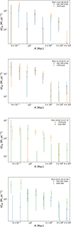 |
Fig. B.1. Reduced excess surface density profiles of Planck clusters detected in multiple public surveys. |
Planck clusters in multiple surveys.
Appendix C: Shear calibration
Shear calibration is regarded as one of the main systematic effects for lensing and we can examine its effect by cross-checking shear estimates. We compare measurements from overlapping survey areas. Direct comparison of ellipticity estimates obtained with different resolution and/or in different band passes might be misleading, as the spatial distribution of the light emission may not be identical and different effective radial weight functions may be used (Schrabback et al. 2018b). However, the estimated reduced tangential cluster shear profile should be consistent when a matched shear catalogue is used (Schrabback et al. 2018b).
In contrast with the main analysis in the paper, for this test we consider cluster samples detected from the same data sets used for shear measurements. This maximises the relevant difference in signal. Source selection is performed based on the photo-z or colours of the reference survey. Any difference in signal between the samples can be only due to differently measured and calibrated galaxy shear.
We compare ellipticity measurements from a reference survey with a comparison survey under two different schemes. We use either identical weights from the reference survey, or we apply each respective survey weights consistently for that survey. Results are summarised in Table C.1. Agreement between HSC-SSP S16a and KiDS DR4, see Figs. C.1, C.2, or CHFTLenS, see Fig. C.3, is good, with differences consistent with zero within the statistical uncertainty.
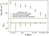 |
Fig. C.1. Average reduced excess surface density profiles of clusters detected by CAMIRA in the fields covered by HSC-SSP S16a and KiDS DR4. Top panel: Average profiles. Bottom: Differences. |
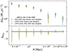 |
Fig. C.3. Average reduced excess surface density profiles of clusters detected by AMICO in the XXL-North field covered by HSC-SSP S16a and CFHTLenS. Top panel: Average profiles. Bottom: Differences. |
Systematic error budget on the shear calibration for WL cluster analyses in Stage-III surveys or precursors.
All Tables
Comparison of the average reduced excess surface density profiles of the Planck clusters detected in different surveys.
Comparison of the average reduced excess surface density profiles of the redMaPPer clusters detected in different surveys.
Comparison of Planck cluster masses from the COMB-CL analysis of public surveys with literature values.
Comparison of redMaPPer cluster masses from the COMB-CL analysis of public surveys with literature values.
Number of redMaPPer clusters per survey with (S/N)WL larger than a given threshold.
Systematic error budget on the mass calibration for WL cluster analyses in Stage-III surveys or precursors.
Systematic error budget on the shear calibration for WL cluster analyses in Stage-III surveys or precursors.
All Figures
|
Fig. 1. Sky coverage in the equatorial coordinate system of the lensing surveys used in this work. We consider only the tiles with sufficiently reliable shape and photo-z measurements. |
| In the text | |
|
Fig. 2. Normalised distribution of the photo-zs up to zp = 2 for selected sources behind a lens plane at zlens = 0.4. The sources are selected either with robust cuts in photo-z or in colour-colour space. |
| In the text | |
|
Fig. 3. Average reduced excess surface density profiles of clusters detected in public surveys as a function of R, the transverse proper distance from the lens centre, coded by colours as in the legend. Top: PSZ2 clusters. Bottom: Sample of redMaPPer. |
| In the text | |
|
Fig. 4. Maximum likelihood estimates of M200c of clusters as obtained with the COMB-CL analysis of public surveys (colour-coded according to the legend) versus literature masses from the LC2 catalogue. Top: PSZ2 clusters. Bottom: Sample from redMaPPer. |
| In the text | |
|
Fig. 5. Binned distribution of (S/N)WL of clusters that lie in public surveys, coded by colour as in the legend. Top: PSZ2 clusters. Bottom: Sample from redMaPPer-SDSS. |
| In the text | |
|
Fig. 6. Binned distribution of (S/N)WL of the candidate clusters detected by AMICO in the XXL-North field covered by HSC-SSP S16a. |
| In the text | |
|
Fig. 7. (S/N)WL of the clusters and groups detected by AMICO in the XXL-North field of HSC-SSP. Top: (S/N)WL as a function of redshift and richness. The (S/N)WL is computed as the median value for the candidate groups in the bin, and (S/N)WL is colour-coded as shown in the right bar. The number of candidates is superimposed in each bin. Bottom: Same as in the top panel for (S/N)WL as a function of redshift and (S/N)det. In other words, this panel shows the S/N of the optical detection of the algorithm. |
| In the text | |
|
Fig. 8. Expected mass thresholds for WL mass precision with Euclid as a function of redshift. For each redshift, we plot the minimum mass for which the mean (S/N)WL is expected to exceed a threshold in the reference cosmology. For comparison, we also show the result from Andreon & Bergé (2012) for a different (S/N)WL definition. |
| In the text | |
|
Fig. 9. Expected number of clusters (in small redshift bins of Δz = 0.001) with (S/N)WL in excess of a given threshold. We show results for different (S/N)WL thresholds (three, five, ten); halo mass function modelling, either from Tinker et al. (2008) or Despali et al. (2016); and cosmological models (the reference one or Planck18). |
| In the text | |
|
Fig. A.1. Structure of the Euclid combined cluster and weak-lensing pipeline, COMB-CL. White parallelograms show input or output products, and blue boxes show COMB-CL modules that perform different processing steps. |
| In the text | |
|
Fig. B.1. Reduced excess surface density profiles of Planck clusters detected in multiple public surveys. |
| In the text | |
|
Fig. C.1. Average reduced excess surface density profiles of clusters detected by CAMIRA in the fields covered by HSC-SSP S16a and KiDS DR4. Top panel: Average profiles. Bottom: Differences. |
| In the text | |
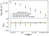 |
Fig. C.2. Same as Fig. C.1 but for AMICO-KiDS-DR3 clusters. |
| In the text | |
|
Fig. C.3. Average reduced excess surface density profiles of clusters detected by AMICO in the XXL-North field covered by HSC-SSP S16a and CFHTLenS. Top panel: Average profiles. Bottom: Differences. |
| In the text | |
Current usage metrics show cumulative count of Article Views (full-text article views including HTML views, PDF and ePub downloads, according to the available data) and Abstracts Views on Vision4Press platform.
Data correspond to usage on the plateform after 2015. The current usage metrics is available 48-96 hours after online publication and is updated daily on week days.
Initial download of the metrics may take a while.