| Issue |
A&A
Volume 696, April 2025
|
|
|---|---|---|
| Article Number | A227 | |
| Number of page(s) | 10 | |
| Section | Cosmology (including clusters of galaxies) | |
| DOI | https://doi.org/10.1051/0004-6361/202553989 | |
| Published online | 25 April 2025 | |
Self-similarity of the mass distribution in rich galaxy clusters up to z∼1 tracked with weak lensing
1
INAF – Osservatorio di Astrofisica e Scienza dello Spazio di Bologna, Via Piero Gobetti 93/3, I-40129 Bologna, Italy
2
INFN, Sezione di Bologna, viale Berti Pichat 6/2, I-40127 Bologna, Italy
⋆ Corresponding author: This email address is being protected from spambots. You need JavaScript enabled to view it.
Received:
31
January
2025
Accepted:
18
March
2025
Abstract
In the standard theory of growth of nonbaryonic dark matter, cosmic structures form hierarchically and self-similarly from smaller clumps. The assembly merger tree extends from the linear perturbations in the early Universe to highly non-linear structures at late times. Gravity is the driving force, and self-similarity should inform cosmic haloes. However, it is unclear whether the apparent anomalies at non-linear scales are due to baryonic or new physics. I show that the mass distribution of rich haloes evolved self-similarly at least since the Universe was 5.7 Gyr old. Using gravitational weak lensing, I constrained the mass profiles of galaxy clusters with M200c ≳ 2 × 10¹⁴ M⊙ that were optically detected in the HSC-SSP survey in the redshift range 0.2 ≤ z < 1.0. The cluster self-similarity confirms the standard theory of growth in the non-linear regime. Clusters are still growing, but neither violent mergers nor matter slowly falling in from the cosmic web disrupt the self-similarity, which is in place well before the halo formation time. Dark matter growth can fit the fossil cosmic microwave background as well as young, very massive haloes. Next-generation survey searches at scales in clusters in which self-similarity breaks might pose a new challenge to dark matter.
Key words: gravitational lensing: weak / galaxies: clusters: general / cosmology: observations / dark matter
© The Authors 2025
 Open Access article, published by EDP Sciences, under the terms of the Creative Commons Attribution License (https://creativecommons.org/licenses/by/4.0), which permits unrestricted use, distribution, and reproduction in any medium, provided the original work is properly cited.
This article is published in open access under the Subscribe to Open model. This email address is being protected from spambots. You need JavaScript enabled to view it. to support open access publication.
1. Introduction
In the standard cold dark matter with a cosmological constant Λ (ΛCDM) cosmology, the cosmic structure grew by gravity out of departures of the primeval mass distribution from homogeneity (Peebles 2025; Efstathiou 2025; Madhavacheril 2025). The agreement between linear perturbation theory and measurements of thermal cosmic microwave background (CMB) radiation at redshift z ∼ 1000 offers a substantial piece of evidence for the model. CMB lensing, which is mainly caused by matter at z ∼ 2, is consistent with the value inferred from the primary anisotropies. In contrast, late-time evolution and non-linear scales probed by weak-lensing measurements from cosmic shear surveys show some differences that might be reconciled if yet to be understood processes suppress the amplitude of the non-linear spectrum on small scales. Currently, it is unclear whether the discrepancies are due to observational systematics, baryonic effects that are not adequately explained, or new physics (Efstathiou 2025; Madhavacheril 2025).
Galaxy clusters stand at the other end of the growth spectrum (Voit 2005). The CMB is a fossil, and clusters are young and still growing. As the latest and most massive nearly virialised haloes to form, their properties place important constraints on cosmological formation theories.
Galaxy clusters are unique laboratories for probing DM and provided the first evidence for it (Zwicky 1937). The validation of the ΛCDM model with an abundance of galaxy clusters would be another strong confirmation in the non-linear regime. Some results from cluster count analyses (Planck Collaboration XX 2014; Planck Collaboration XXIV 2016; Costanzi et al. 2021) differed from multiple cosmological probes, for example, supernovae, baryon acoustic oscillations, cosmic shear, galaxy clustering, or CMB anisotropies. However, other cluster analyses did not support previous results (Lesci et al. 2022; Bocquet et al. 2024; Ghirardini et al. 2024). More than signs of physics beyond the ΛCDM model, the differences might be due to unaccounted for systematic uncertainties related to incomplete or impure samples or to biased mass calibration.
Cosmological information is encoded in the mass distribution of galaxy clusters. In the standard scenario, structure grows hierarchically. The massive DM haloes that host massive clusters have assembled through a process that depends on the cosmic matter content, expansion rate, and on the amplitude of initial matter density fluctuations (Corasaniti et al. 2022). First tests based on sparsity, that is, the ratio of the halo mass within radii enclosing different over-densities, are nearly insensitive to selection or mass calibration biases and provide constraints that agree with primary CMB analyses (Corasaniti et al. 2021).
The density fluctuations that give rise to massive clusters are approximately scale-free and result in a self-similar evolution apart from dissipative processes (Kaiser 1986). The formation of bound, virialised structures in an expanding Universe can be described as the spherical collapse of positive density perturbations (Gunn & Gott 1972). Bound shells continue to turn around and fall in. The secondary infall approaches self-similaritiy and informs the halo mass distribution (Gunn 1977; Fillmore & Goldreich 1984; Bertschinger 1985).
However, the collapse of peaks is generally expected to be non-spherical and to follow the preferential direction of the filamentary structure of the cosmic web. Numerical simulations of DM haloes can recover the merger tree of cosmic structure formation, as clumps of matter merge to form larger clumps in a hierarchy of mergers that continued to the formation of galaxies and groups and clusters of galaxies as galaxy merging slowed. Simulations have shown that the growth of DM halo density profiles undergoes two major phases (Navarro et al. 1997; Bullock et al. 2001; Zhao et al. 2003; Wechsler et al. 2002; Diemer & Kravtsov 2014; Fujita et al. 2018). In the early stages, the accretion is fast, and mass builds up in the central region of the cluster. In a later, slow accretion phase, the mass builds in the outer region while the mass density in the core remains approximately constant (Gott & Rees 1975; Gunn 1977; Łokas & Hoffman 2000; Ascasibar et al. 2004, 2007; Lithwick & Dalal 2011).
The numerical study of galaxy clusters at high redshift is a computationally demanding task, as simulations have to resolve the inner regions of the clusters down to small scales, and at the same time, they need to correctly reproduce the influence of the large-scale structure on the outer, gravity-dominated regions. First results confirmed self-similarity (Le Brun et al. 2018; Mostoghiu et al. 2019; Singh et al. 2025). The evolution of the density profiles of the 25 most massive galaxy clusters in a DM Universe, once scaled to the critical density, exhibits low dispersion and little evolution up to redshifts z ∼ 1 (Le Brun et al. 2018), suggesting that self-similarity was established early in the formation process. This was confirmed by tracking the merging history of the 300 most massive clusters at z = 0 backwards in time (Mostoghiu et al. 2019). The mass distribution of the progenitors is already in place by z ∼ 2.5.
The complex behaviour of baryons can hamper self-similarity in galaxies or small groups. Because they are dominated by DM with a baryonic fraction in line with the universal value, massive galaxy clusters offer a useful laboratory for DM tests. As highly non-linear structures, they might be difficult to model, but in the new era of precision astronomy, they can be investigated with many tools.
The main baryonic components consists of a hot, X-ray emitting intracluster medium (ICM). The bulk of the ICM outside the inner core in massive clusters has evolved self-similarly since z ∼ 1.9, as tracked by X-ray inferred gas density profiles and thermodynamic properties (McDonald et al. 2017; Ghirardini et al. 2021). This indicates the self-similar evolution of the underlying DM distribution, since rich clusters are DM dominated, and the gas distribution, except in the very central regions, is driven by gravity.
I directly measure the self-similarity of the matter profiles of rich clusters by detecting the weak-lensing (WL) signal. The theory of WL by galaxy clusters is well understood (Bartelmann & Schneider 2001; Umetsu 2020). WL distorts the shape of the background galaxies and the shear profile accurately, and it precisely tracks the total mass distribution of the lens (Hoekstra et al. 2012; von der Linden et al. 2014; Applegate et al. 2014; Hoekstra et al. 2015; Umetsu et al. 2014, 2016; Okabe & Smith 2016; Dietrich et al. 2019). WL provides a direct measurement of the excess surface mass density of the cluster acting as a lens, and no assumptions about the dynamical status or the equilibrium between baryons and DM are required.
Until relatively recently, WL analyses were only possible with dedicated, targeted observations (von der Linden et al. 2014; Umetsu et al. 2014), which made the study of statistically complete, homogeneous, and large samples elusive. Photometric surveys have now advanced to the so-called Stage-III (Albrecht et al. 2006). Based on their ever-increasing depth, the WL signal of cluster samples can now be measured up to high redshifts (Sereno et al. 2017; Umetsu et al. 2020; Melchior et al. 2015; Medezinski et al. 2018; Sereno et al. 2018). Singh et al. (2025) measured the WL signal of galaxy clusters in the area covered by the Dark Energy Survey (DES), which were first selected by the South Pole Telescope thermal Sunyaev–Zel’dovich effect and were then optically confirmed. The authors found some evidence for self-similarity up to z ∼ 0.6. I take advantage of the deepest Stage-III galaxy image survey to search for self-similarity up to z ∼ 1.0.
As a reference cosmological framework, I assumed the concordance flat ΛCDM model with total matter density parameter ΩM = 0.3, baryonic parameter ΩB = 0.05, Hubble constant H0 = 70 km s−1 Mpc−1, power spectrum amplitude σ8 = 0.8, and initial index ns = 1. When H0 is not specified, h is the Hubble constant in units of 100 km s−1 Mpc−1. The suffix Δc refers to the region within which the halo density is Δ times the cosmological critical density at the cluster redshift, ρcr. ‘log’ is the logarithm in base 10, and ‘ln’ is the natural logarithm.
2. The deepest Stage-III survey
The Hyper Suprime-Cam Subaru Strategic Program (HSC-SSP; Miyazaki et al. 2018; Aihara et al. 2018) is the deepest Stage-III galaxy image survey, and it opens a window on cluster physics at high redshift. HSC-SSP is a multi-band imaging survey in five optical bands (g, r, i, z, and y) with HSC, an optical wide-field imager with a field of view of 1.77deg2 mounted on the prime focus of the 8.2 m Subaru telescope (Miyazaki et al. 2018; Komiyama et al. 2018; Furusawa et al. 2018; Kawanomoto et al. 2018). The wide survey is optimised for WL studies (Mandelbaum et al. 2018; Hikage et al. 2019; Miyatake et al. 2019; Hamana et al. 2020), and it aims to observe ∼1200deg2 with a depth of i ∼ 26 mag at the 5σ limit within a 2-arcsecond-diameter aperture (Aihara et al. 2018).
I considered the latest data releases at the time of writing for each product used in the analysis, which are S16a for the shear catalogue (see Sect. 2.1) and S18a for the catalogue of clusters (see Sect. 2.2). The analysis is limited to the clusters in the S16a footprint.
2.1. Shears
I exploited the S16a catalogue of galaxy shape measurements from the first-year data release (Mandelbaum et al. 2018). The catalogue covers an area of ∼137deg2 split into six fields (see Fig. 1), observed to final depth, with a mean i-band seeing of 0.58 arcseconds. Galaxy shapes were estimated on the co-added i-band images (Hirata & Seljak 2003) by fitting a Gaussian profile with elliptical isophotes to the image with a conservative magnitude cut of i < 24.5 mag. The nominal unweighted and weighted source number densities are 24.6 and 21.8 arcmin−2, respectively (Mandelbaum et al. 2018).
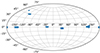 |
Fig. 1. Sky coverage in equatorial coordinates of the lensing survey HSC-SSP S16a. |
My choices for the lensing analysis were informed from previous WL studies (Chiu et al. 2020; Umetsu et al. 2020). Photometric redshifts (photo-z or zp) are well recovered in the redshift range 0.2 ≲ z ≲ 1.5, with an accuracy of σzp/(1 + zp)∼0.05 (0.04), and an outlier rate of ∼15 (8) % for galaxies down to i = 25 (24) (Tanaka et al. 2018). I considered photo-zs measured with the EPHOR_AB code based on point spread function-matched aperture photometry (Tanaka et al. 2018). For the photometric magnitudes, I considered the forced cmodel (Huang et al. 2018).
2.2. Clusters
A complete and homogeneous sample of optically selected clusters was retrieved from HSC-SSP with the cluster-finding algorithm based on multi-band identification of red sequence galaxies (CAMIRA; Oguri et al. 2018). CAMIRA fits each galaxy in the image with a stellar population synthesis model to compute the likelihood that it is a red-sequence galaxy at a given redshift (Oguri 2014; Oguri et al. 2018). Each cluster candidate is assigned a redshift and a richness  , which describes the number of red member galaxies with stellar masses M* ≳ 1010.2 M⊙ and within a circular aperture with a radius R ≲ 1.4 Mpc. The richness is a reliable mass proxy, with an intrinsic scatter of ∼15% at fixed mass (Oguri et al. 2018).
I considered the catalogue version constructed from the public data release 3 (S18a). There are 1439 clusters in the WL footprint at a redshift 0.1 < z < 1.1 and with a richness  , which roughly corresponds to M200c ≳ 1.1 × 10¹⁴ M⊙ (Oguri et al. 2018). The sample is highly pure (≳95%) down to the richness limit of
  , and it is high complete (∼95%) for high-mass clusters M200c ≳ 2 × 10¹⁴ M⊙. The cluster redshift is recovered with a scatter of 0.008 × (1 + z). Nearly 68% of the clusters is well centred, the other clusters show a mean off-set of ∼0.4 Mpc.
I studied the evolution of cluster density profiles in four equally spaced redshift bins from z = 0.2 to 1 (see Fig. 2). In each bin, I selected the 100 richest clusters to focus on the high-mass end of the halo mass function. Clusters at z < 0.2 were excluded from the analysis due to the small comoving volume. Clusters at z ≥ 1 were excluded due to the poor WL signal.
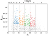 |
Fig. 2. Distribution of the CAMIRA clusters in the redshift – richness plane. The age of the Universe at a given redshift is plotted on the top axis. The points are colour-coded according to their redshift bin. Clusters represented by grey points are excluded from the WL analysis. |
3. Methods
I present the methods I used for the WL inference of mass and shape profiles, for the abundance matching, and to compare the profile. I refer to quoted references for further details.
3.1. Signal definition
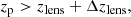
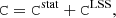
The main observable to constrain density profiles with lensing is the reduced excess surface density ΔΣgt, which can be expressed in terms of the surface density, Σ, and of the excess surface density ΔΣt. For an axially symmetric lens and a single source plane,
 (1)
(1)
where R is the transverse proper distance from the assumed lens centre,  is the mean density within R, and
 (2)
(2)
the critical density for lensing, Σcr, can be expressed as
 (3)
(3)
where c is the speed of light in vacuum, G is the gravitational constant, and Dl, Ds, and Dls are the angular diameter distances to the lens, to the source, and from the lens to the source, respectively.
For a source redshift distribution, the source-averaged reduced excess surface mass density can be approximated as (Umetsu 2020)
 (4)
(4)
The equations presented here and in the following also hold for non-axially symmetric lenses when azimuthally averaged quantities are considered.
3.2. Signal measurement
I measured the reduced excess surface density ΔΣgt in circular annuli with the estimator
 (5)
(5)
where
 (6)
(6)
The sum runs over the sources inside each annulus centred at R, and et, i is the tangential component of the ellipticity of the ith source galaxy, wi is the weight assigned to the source ellipticity, and Σcr, i is the critical density for the ith source.
The shape catalogue I used lists measurements of the distortion δ, which is related to the ellipticity through the responsivity ℛ as (Mandelbaum et al. 2008; Rowe et al. 2015; Kaiser et al. 1995),
 (7)
(7)
The mean responsivity in an annulus can be calculated from the inverse variance weights and the per-object estimates of the RMS distortion δRMS, i as (Mandelbaum et al. 2018),
 (8)
(8)
where ⟨…⟩ΔΣ denotes an average with the wΔΣ, i weights.
I computed distances to the sources and critical surface densities or selected background galaxies based on the photo-z point-estimator. Other methods exploit the per-source photo-z probability density function (Sheldon et al. 2004) or the ensemble source redshift distribution (Hildebrandt et al. 2020). These methods rely on an unbiased and accurate redshift probability distribution, which needs expensive calibration samples or simulations (Tanaka et al. 2018; Hildebrandt et al. 2020). For this analysis, I preferred to rely on conservative selections based on the photo-z point-estimator (Sereno et al. 2017; Medezinski et al. 2018), whose level of systematic errors is under control and subdominant for Stage-III surveys (Bellagamba et al. 2019; Euclid Collaboration: Sereno et al. 2024).
3.3. Background source selection
I selected galaxies behind the lens as sources for the WL analysis based on their photo-z or colours. As a first step, I selected galaxies such that
 (9)
(9)
where zlens is the lens redshift, zp is the source redshift, and Δzlens = 0.1 is a threshold above the cluster redshift to lower the contamination.
In addition to this criterion, I required that the sources passed more restrictive cuts in either photo-z or colour properties, which I discuss below.
3.3.1. Photometric redshifts
A secure population of background galaxies can be selected with criteria based on the photo-zs (Sereno et al. 2017),
 (10)
(10)
 (11)
(11)
 (12)
(12)
 (13)
(13)
where zp, 2.3% is the lower bound of the region including 95.4% of the probability density distribution. The photo-z risk parameter R(zp) represents the expected loss for a given choice of zp as the point estimate, and it quantifies the confidence in the point estimate of the redshift (Tanaka et al. 2018). Thresholds are conservative, and I selected galaxies in the redshift range 0.2 < zp < 1.5, in which photo-z is thought to be reliable (Tanaka et al. 2018). The contamination level is expected to be at the percent level (Oguri et al. 2012; Sereno et al. 2017; Medezinski et al. 2018; Umetsu et al. 2020).
3.3.2. Colour–colour
The selection of galaxies in colour–colour space can provide complete and pure background samples and can complement the photo-z selection (Euclid Collaboration: Lesci et al. 2024). I adopted the cuts in the g − i versus r − z colour–colour space (Medezinski et al. 2018), which are optimised for the HSC-SSP. Blue or red galaxies are efficiently separated in this space for lenses up to zlens ≲ 1.1. The level of contamination is within the percent level (Medezinski et al. 2018; Euclid Collaboration: Lesci et al. 2024).
3.4. Shear calibration
The raw shape components of the source galaxies, eraw, 1 and eraw, 2, can be affected by a multiplicative (m) or an additive (c) bias,
 (14)
(14)
HSC-SSP calibrated the bias with simulations (Mandelbaum et al. 2018). I corrected each galaxy shape for the additive bias, whereas the multiplicative bias m was averaged in each annulus (Heymans et al. 2012; Miller et al. 2013; Viola et al. 2015),
 (15)
(15)
3.5. Rescaling
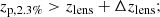
When I compared lensing profiles, I rescaled the lengths by a proxy for the over-density radius,
 (16)
(16)
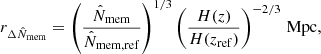
where the pivots were fixed to  and zref = 0.6.
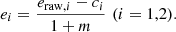
For each cluster, I measured the lensing signal ΔΣgt in eight radial circular annuli equally separated in logarithmic space that spanned the range between 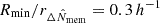 (∼0.43) and
 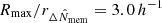 ( ∼ 4.3) from the cluster centre.
The surface densities were scaled by
 (17)
(17)
3.6. Noise
The uncertainty covariance matrix for a single lens accounts for measurement uncertainties and lensing from the uncorrelated large-scale structure (LSS), ΔΣLSS,
 (18)
(18)
where Cstat accounts for the shape noise and shear measurements uncertainties, and CLSS is the covariance due to LSS. The main source of noise is the intrinsic ellipticity dispersion σeα. For Stage-III surveys and optical bands, σeα ≃ 0.26 − 0.3 (Schrabback et al. 2018; Euclid Collaboration: Martinet et al. 2019; Euclid Collaboration: Ajani et al. 2023).
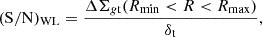
The covariance CLSS accounts for lensing from LSS (Hoekstra 2003; Sereno et al. 2018). It can be written as the cross-correlation between two angular bins Δθi and Δθj (Schneider et al. 1998; Hoekstra 2003),
 (19)
(19)
where Pk(l) is the effective lensing-projected power spectrum. I computed the linear matter power spectrum with a semi-analytical fitting function (Eisenstein & Hu 1998) and the effects of non-linear evolution with the revised halofit model (Takahashi et al. 2012). These approximations are adequate for the precision needed in my analysis. The function g is the filter. In an angular bin θ1 < Δθ < θ2,
![Mathematical equation: $$ \begin{aligned} g=\frac{1}{\pi (\theta _1^2 -\theta _2^2)l} \left[ \frac{2}{l} \left( J_0(l \theta _2) -J_0(l \theta _1) \right) +\theta _2 J_1(l \theta _2) -\theta _1 J_1(l \theta _1) \right]. \end{aligned} $$](/articles/aa/full_html/2025/04/aa53989-25/aa53989-25-eq27.gif) (20)
(20)
I did not consider correlated noise due to the intrinsic alignment of the sources, which can be neglected for Stage-III analyses of cluster lensing (McClintock et al. 2019; Umetsu et al. 2020), or the correlated large-scale structure, which is subdominant in the radial range I considered (McClintock et al. 2019; Euclid Collaboration: Sereno et al. 2024).
For my reference analysis, I assumed that lensing signals between lenses were uncorrelated. My sample consisted of 400 clusters in an area of ≲140deg2, with an average projected separation in the plane of the sky of ∼0.6deg. This is larger than the radial extension for the shear profiles under consideration, which cover ≲0.2deg (≲0.4deg) at the median (minimum) redshift of the sample.
3.7. Signal-to-noise ratio
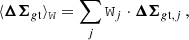
The signal-to-noise ratio (S/N) of the WL profile can be defined in terms of the weighted excess surface density ΔΣgt in the relevant radial range Rmin < R < Rmax (Sereno et al. 2017),
 (21)
(21)
where the noise δt includes statistical uncertainties and cosmic noise. I measured (S/N)WL between Rmin = 0.3 h−1 Mpc and Rmax = 3.0 h−1 Mpc from the cluster centre.
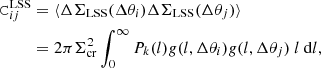
3.8. Population averages and covariances
I computed the average lensing profiles and the related covariance matrix. The covariance can be computed theoretically, analytically, or by resampling. For this analysis, I considered the latter two methods.
3.8.1. Analytical
The weighted average of the lensing profiles of a population of lenses in a redshift bin, ⟨ΔΣgt⟩W, can be measured with standard statistical methods as (Schmelling 1995)
 (22)
(22)
with weight matrices Wj,
 (23)
(23)
where Cjj is the covariance matrix of the jth lensing profile ΔΣgt, j. For the present analysis, Cii is non-diagonal to the LSS noise.
The weighted covariance matrix for the average can be written as
 (24)
(24)
where Cij is the cross-covariance between the ith and jth lens. For the reference analysis, the cross-covariance between different lenses (i ≠ j) was assumed to be null.
Together with the measurement uncertainties, scatter due to rescaling should also be accounted for. The richness is a scattered proxy of the mass. If the mass is overestimated, the profile is rescaled to a lower value of R/rΔ than expected, and at the same time, the value of ΔΣgt/ΣΔ is biased low. The scatter in the proxy over-density radius,  , can be written as
 (25)
(25)
where Nav is the number of averaged clusters, and  is the proxy scatter (Oguri et al. 2018). The scatter in the rescaling unit
  is a source of scatter for the rescaled profiles. If the lensing profile has a logarithmic slope equal to γR, ΔΣt ∝ R−γR, the associated covariance matrix can be written as
 (26)
(26)
Cδ is subdominant with respect to CW, and a nearly isothermal profile with γR = 1 can be safely assumed.
3.8.2. Resampling
Covariance matrices can be alternatively computed with internal estimators that directly resample the observed data by using, for example, a jackknife or bootstrap method to generate multiple copies of the observations (Mohammad & Percival 2022). The added value of these approaches is that they account for all systematic or statistical uncertainties and correlations, including cross-correlations between redshift or richness bins, which are estimated with a data-driven approach. On the other hand, the inverse of a noisy, unbiased estimator of the covariance matrix is not an unbiased estimator of the inverse covariance matrix (Hartlap et al. 2007; Mandelbaum et al. 2013), and corrections or calibrations might still be needed.
For the survey under study, I considered the analytical covariance as the reference covariance mostly due to the small sample (only 400 clusters) and limited survey area (≲140 deg2). However, to validate the result, I also computed the covariance matrix by bootstrap resampling with a replacement. I grouped the lenses in simply connected regions (McClintock et al. 2019). I considered 50 groups, so that there were two clusters from any redshift bin per group on average, and I resampled over the lens groups 104 times. I resampled over the lenses, that is, the lensing profiles, rather than over the sources (which would need a recomputation of the lensing profiles at each step), but except for subdominant border effects for clusters near the spatial region edges, the two different resamplings provided comparable results.
3.9. Profile comparison
The self-similarity of populations a and b was tested by comparing average lensing profiles,
 (27)
(27)
where the difference between the profiles can be written as
 (28)
(28)
and the total uncertainty covariance for the difference accounting for shape noise, LSS, and systematics in the rescaling isgiven by
 (29)
(29)
The null hypothesis is that the profiles are self-similar, that is, Δab is consistent with a null signal. The p-value used as metric for comparison was computed as the probability for a χ2 distribution with Nd.o.f. degrees of freedom to exceed the measured value, p(χ2 > χa, b2; Nd.o.f.). Here, Ndof equals the number of radial bins. A very low p-value, that is, a large χa, b2 compared to Nd.o.f., means that the observed profiles would be very unlikely if they were self-similar (null hypothesis).
3.10. Abundance matching
The properties of a cluster sample can be estimated by matching its abundance with the expected abundance of haloes for a given cosmological model (Rykoff et al. 2012; Oguri et al. 2018; Murata et al. 2019). I first simulated a population of haloes in the ΛCDM framework, then I computed mock observable properties, and I finally matched the simulated to the observed clusters.
I simulated clusters from the cosmological halo massfunction,
 (30)
(30)
where n is the number density, and V is the comoving volume. I modelled the halo mass function as in Tinker et al. (2008). In an area equal to the area covered by the survey, I expect ∼3000 haloes with a mass higher than 10−13.9 M⊙ between z = 0.15 and z = 1.05 in the reference cosmology. The total number of simulated clusters was extracted from a Poisson distribution centred on the mean value.
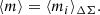
I selected clusters according to a mass proxy NM related to the true halo mass as
 (31)
(31)
where 𝒩 is the normal distribution. The distribution was centred on the true value, and it had the same scatter as the measured conditional scatter of the (logarithm of the) richness at a given mass,  , see Sect. 2.2.
I accounted for the uncertainty in the observed cluster redshift as
 (32)
(32)
where σz = 0.008 × (1 + z) (see Sect. 2.2). The clusters were assigned to their redshift bin based on zobs.
For each redshift bin, I selected the richer clusters, that is, the clusters with higher values of NM. Completeness was simulated by considering the 100/C richer clusters, where C is the completeness, and randomly drawing 100 of them. The CAMIRA cluster sample is highly complete for massive haloes. I assumed a sample completeness of C = 0.95.
I finally studied the mass distribution of the selected clusters. I performed 104 simulations.
3.11. Halo model
Cluster masses can be measured by fitting the lensing profiles in a fixed cosmological model (Sereno et al. 2017; Umetsu 2020). I only discuss the specific setting adopted for the present analysis. The excess surface density profile of the stacked lenses can be modelled as (Johnston et al. 2007)
 (33)
(33)
where ΔΣcen is the excess surface density contributed by the centred haloes, fmis is the fraction of miscentred clusters, and ΔΣmis is the excess surface density of the miscentred haloes.
The well-centred haloes are described with ΔΣcen. I modelled the lenses with Navarro, Frenk, White profiles (NFW; Navarro et al. 1996) that were characterised by a mass of M200c and a concentration of c200c. As fitting parameters, I considered the logarithm (base 10) of the mass and concentration, p = (logM200c, logc200c). Here, logM200c is short for log10[M200c/(1014 M⊙)].
Cluster detection algorithms might misidentify the cluster centre, or the optically detected centre might differ from the minimum of the gravitational potential. Miscentering leads to an underestimate of ΔΣt(R) at small scales and to a low bias on the measurement of the concentration. The azimuthally averaged surface density of a halo that is misplaced by Rmis from the centre of the lens plane can be computed as (Yang et al. 2006)
 (34)
(34)
where Σcen is the centred profile. I modelled the distribution of the off-sets with an azimuthally symmetric Gaussian distribution (Johnston et al. 2007; Hilbert & White 2010),
![Mathematical equation: $$ \begin{aligned} P(R_{\rm mis})=\frac{R_{\rm mis}}{\sigma _{\rm mis}^2}\exp \left[ -\frac{1}{2}\left( \frac{R_{\rm mis}}{\sigma _{\rm mis}}\right)^2 \right], \end{aligned} $$](/articles/aa/full_html/2025/04/aa53989-25/aa53989-25-eq46.gif) (35)
(35)
where σmis is the scale length. The contribution of the off-centred haloes is then
 (36)
(36)
For the CAMIRA clusters, the typical scale length is about σmis ∼ 0.4 Mpc (Oguri et al. 2018).
3.12. Weak-lensing mass inference
The lens parameters were fitted with a Bayesian analysis (Euclid Collaboration: Sereno et al. 2024). The posterior probability density function of the parameters, p, given the data, {⟨ΔΣgt⟩}, is written as
 (37)
(37)
where p is a vector including the model parameters, ℒ is the likelihood, and pprior is the prior. I considered non-informative priors with −1 ≤ logM200c ≤ 2, 0 ≤ logc200c ≤ 1, 0 ≤ foff ≤ 0.5, and 0.1 ≤ σs/(1 Mpc)≤0.7.
The likelihood is ℒ ∝ exp(−χ2/2), where χ2 is written as
![Mathematical equation: $$ \begin{aligned} \chi ^2 = \sum _{i,j} \left[ \langle \Delta \Sigma _{g\mathrm{t}}\rangle _i - \Delta \Sigma _{g\mathrm{t}} (R_i | \boldsymbol{p}) \right]^\mathrm{t} \mathtt C _{ij}^{-1} \left[ \langle \Delta \Sigma _{g\mathrm{t}}\rangle _j - \Delta \Sigma _{g\mathrm{t}} (R_j | \boldsymbol{p}) \right] \end{aligned} $$](/articles/aa/full_html/2025/04/aa53989-25/aa53989-25-eq49.gif) (38)
(38)
the sum extends over the radial annuli, ΔΣgt(Ri|p) is the halo model computed at the lensing weighted radius Ri of the ith bin (Sereno et al. 2017), and ⟨ΔΣgt⟩i is the measured reduced excess surface density in the ith bin.
4. Results
I studied the properties of the observed clusters and how they fit in the ΛCDM framework.
4.1. Masses
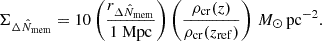
The summary statistics for the masses estimated with abundance matching, MAM, for each redshift bin are listed in Table 1. The expected mass distributions are shown in Fig. 3. Since the richness is a nearly unbiased, time-independent proxy of the mass, a cut in richness results approximately in a cut in mass at M200c ≳ 1.5 × 10¹⁴ M⊙. The mass distribution is also nearly independent of time independent (see Fig. 3), and it peaked at M200c ∼ 3 × 10¹⁴ M⊙.
 |
Fig. 3. Mass distribution of the selected clusters in redshift bins as estimated by the abundance matching. The distributions are coded by colour and line style according to the redshift bin. |
Mass properties of the selected CAMIRA clusters for the redshift bin.
I measured the WL signal in circular annuli. The average excess surface density profiles are shown in Fig. 4. The lensing signal is recovered with high signal-to-noise, S/NWL, in each redshift bin, see Table 1.
 |
Fig. 4. Average reduced excess surface density profiles of massive CAMIRA clusters as a function of distance from the lens centre. The lengths and densities are rescaled by over-density units. The vertical error bars represent the square root of the diagonal elements of the total uncertainty covariance matrix, including statistical and LSS noise. The profiles are coded by colour and style according to the cluster redshifts, as in the legend, and they are horizontally shifted by 2% along the abscissa for clarity. |
The typical mass in each redshift bin can be directly inferred by fitting the measured lensing profile with a parametric lens model (see Sect. 3.12). The cluster mass distribution can be recovered with the WL analysis of the excess surface density ΔΣgt. All the matter along the line of sight contributes to the lensing phenomenon. In a stacked sample of lenses, there are three main contributors: (i) The centred lenses, that is, the collapsed and nearly virialised clusters, whose signal can be well recovered up to radii ≲3 Mpc, and whose centre is well determined (see Sect. 3.11); (ii) clusters with the same properties as the centred ones, but whose estimated centres are measured with an off-set distribution (see Sect. 3.11); and (iii) the uncorrelated matter of the LSS that fills the line of sight and contributes noise (see Sect. 3.6). The halo model was then fitted to the lensing profiles (in proper units) to give a direct estimate of the WL mass.
The WL masses (see Table 1), agree well with estimates from abundance matching, which is a comforting confirmation for the tested cosmological scenario. The difference between the WL mass of the mean profile and the mean mass of the abundance-matched clusters is comparable to the statistical uncertainty of the WL mass and it is smaller than the scale on the expected distribution in mean mass from abundance matching. Due to the still limited survey area and the rarity of massive clusters, the maximum mass from abundance matching can strongly vary among different realisations of the simulated survey. On the other hand, the minimum mass, which is better sampled, is estimated with a better precision. For any deviation from ΛCDM to emerge as a difference between the estimated mass from either WL or abundance matching, a larger survey area is needed.
4.2. Self-similar density profiles
The mass density profile is thought to be self-similar in a ΛCDM scenario when the radial and density units are rescaled by the over-density radius and the critical density of the Universe at the cluster redshift, respectively (Le Brun et al. 2018). The richness is a reliable proxy for the mass, and it can be used to define units for rescaling,  and
and  for the length and surface density, respectively (see Sect. 3.5). This can add additional scatter (see Sect. 3.8), but makes our results independent of the WL-inferred mass inference, which could reduce possible time-evolution, and of the halo model.
The agreement between the profiles is good (see Fig. 4), with no sign of redshift evolution. I quantified the level of agreement between signals from different redshift bins with a p-valuestatistics (see Sect. 3.9). All profiles are consistent within the statistical uncertainties, with no signs for evolution (see Table 2).
Comparison of the average reduced excess surface density profiles in different redshift bins.
The self-similarity between profiles is still recovered when the uncertainty covariance is computed with a bootstrap resampling of clusters grouped in spatially connected regions of the survey area. Notwithstanding the noisy covariance matrix, the average p-value is ∼0.15.
I excised from the analysis the cluster region within ≲0.4 Mpc since the measured signal here could deviate from self-similarity. Firstly, miscentring can flatten the profile and might cause an apparent breaking of the self-similarity. Secondly, in a two-phase accretion model for halo mass growth, material falling in remains in the outer regions, while the core evolves almost unperturbed. Since the inner regions are also the most contaminated, I conservatively chose not to include them in the WL analysis. With an even more conservative excision of the regions up to ∼0.57 Mpc, the p-values improve by ∼ + 0.13 on average.
Since in each redshift bin the signal is dominated by clusters of similar mass, M200c ∼ 3 × 10¹⁴ M⊙ (see Fig. 3), self-similarity should be still in place when the signal is stacked in comoving (Umetsu et al. 2020) or proper units. This is in fact the case, as the average p-values decrease by ∼ − 0.15 or ∼ − 0.24 for comoving or proper units, respectively, but at ∼0.54. or ∼0.46, they are still consistent with self-similarity. At a fixed mass, rescaling in comoving units captures most of the self-similarity.
4.3. Mass-accretion history
My sample consisted of the most massive clusters in the redshift and area volume covered by HSC-SSP S16a. It does not track an evolutionary sequence. The massive CAMIRA clusters at z ∼ 1.0 are not the progenitors of the low-redshift clusters at z ∼ 0.2. Their descendants are more massive, but they can be missed mostly due to the small volume of the observed local Universe. In models for the mass-accretion history of DM haloes, clusters can be placed on an evolution track. The formation redshift zform can be defined as the redshift where the main halo progenitor has accreted one -half of the expected final mass at z = 0 (Mostoghiu et al. 2019).
Correa et al. (2015) used the extended Press-Schechter formalism to derive the halo mass-accretion history from the growth rate of initial density perturbations. I used their model to compute the mass of the main progenitor along the main branch of the merger tree as a function of redshift. I took as starting point the mass and redshift estimated from WL for the average profile and placed a halo with this mass and redshift on an accretion track to predict its final mass at z = 0 or to trace it back in time and estimate its formation redshift.
The clusters in my sample experienced different phases of their accretion history (see Table 1). The clusters in the sample up to z ≲ 0.5 are observed after their formation redshift, the clusters at z ∼ 0.7 are nearly at their formation time, that is, nearly halfway in their mass-accretion process, whereas clusters at z ∼ 0.9 are caught nearly 1.3 Gy before zform, when they still have to accrete about two-thirds of their final mass by major mergers or slow inflow. Notwithstanding the very different evolution phases, the clusters in my sample show self-similar mass profiles up to z ∼ 1.
4.4. Summary
The WL inferred properties of the most massive optically detected clusters in HSC-SSP S16a provide a picture that is consistent with the standard theory of structure formation.
-
The WL mass of the richest optically selected haloes matches the prediction from ΛCDM well.
-
The halo mass distribution as inferred from the excess surface density profiles is remarkably self-similar up to z ∼ 1.
-
Substantial self-similarity is attained in the early stages of the formation process, before the main progenitor still has to accrete one-half of the expected final mass.
5. Systematics
The total level of systematic uncertainty that affects the calibration of the excess surface density for HSC-SSP 16a is about ≲3% (Murata et al. 2019; Umetsu et al. 2020). The main sources of systematic errors are shear calibration, photo-z uncertainties, contamination due to foreground or member galaxies, and modelling effects. This level of accuracy is adequate for the precision of my profiles, which are constrained at the level of 5–10% in the redshift bins with the best (S/N)WL.
The analysis I presented relied on constraints on the redshift evolution more than on the absolute calibration, and a constant level of systematics, if it were redshift independent, would not affect our analysis. The selection of background galaxies was conservative and secure in the explored redshift range. The bias, scatter, and outlier fraction for the photo-zs are nearly constant up to zp = 1.5 (Tanaka et al. 2018), which is the maximum source redshift I employed.
Shear is calibrated at the percent level (Mandelbaum et al. 2018). Furthermore, the calibration of selected sources is nearly redshift independent, as found by comparing the multiplicative bias for lenses at different redshifts. For clusters at z = 0.3, 0.5, 0.7, and 0.9, I find a weighted multiplicative bias of background sources of ⟨m⟩= − 0.12 ± 0.9, −0.12 ± 0.9, −0.12 ± 0.9, and −0.13 ± 0.9. A time-independent multiplicative bias is consistent with the data.
Contamination is also expected to be under control. I excised from the analysis the innermost regions within a minimum distance radius of R ≳ 0.4 Mpc, which removed most of the contamination from the member galaxies.
In summary, systematics are expected to be subdominant with respect to the statistical precision. Different residual effects are expected to be uncorrelated among them, and each effect is expected to be correlated among different redshifts bins, which neither disrupt nor enhance self-similarity.
6. Conclusions
The growth of the nonbaryonic DM theory can explain both the CMB anisotropies in the liner regime or the density profiles of massive haloes in the highly non-linear regime. The list of current anomalies is intriguing but significantly shorter than the body of evidence supporting the theory (Peebles 2025). As far as DM and gravity are the main drivers of formation and evolution, the theory is very successful. The differences mostly arise in non-linear regimes where baryonic effects become significant and can compete with gravity (Efstathiou 2025; Madhavacheril 2025). The theory is apparently paradoxical because the matter that is dark is easy to model, whereas the matter that is luminous and familiar undergoes mechanisms that are difficult to grasp. It works, however.
The self-similarity of galaxy clusters is a strong prediction of CDM (Kaiser 1986). Simulations found that notwithstanding the variety of dynamical states and formation histories, the density profiles of the most massive haloes in the Universe, once scaled by the critical density, are remarkably similar and converge quickly to the near-universal form displayed by relaxed systems in the local Universe (Le Brun et al. 2017; Mostoghiu et al. 2019; Singh et al. 2025).
The observation of galaxy clusters with gravitational lensing showed that the mass distribution in clusters was already established when the Universe was ∼5.7 Gyr old and that the evolution has been self-similar since then. Merger activity and matter infall do not disrupt the density profiles, which are already stable at z ∼ 1. Self-similarity is in place before the cluster formation time, which for the massive clusters in our sample is zform ∼ 0.6 − 0.7.
The DM history in rich clusters differs from the hot gas, which takes some time to reach equilibrium (Sereno et al. 2021). The thermalisation epoch follows the cosmic DM – dark energy equality at z ∼ 0.33, and lies in a gentler era of structure growth. Even though the distribution of the ICM in massive clusters has evolved self-similarly since z ∼ 1.9 (McDonald et al. 2017; Ghirardini et al. 2021), the most massive clusters in the observed Universe attained an advanced thermal equilibrium only ∼1.8 Gyr ago, at redshift z = 0.14 ± 0.06, when the Universe was 11.7 ± 0.7 Gyr old (Sereno et al. 2021). The DM profiles were already established at z ≳ 1 (when the Universe was ≲5.7 Gyr old) in an early phase of the cluster growth.
Self-similarity in clusters could break in the cluster cores, which evolve nearly unperturbed in a two-phase accretion process, or in the outskirts, where matter is still falling in from the cosmic web. We should be able to investigate these regimes with the final phase of Stage-III surveys when HSC-SSP will be complete, or with the first phase of Stage-IV surveys, which started with the successful launch of the Euclid satellite (Euclid Collaboration: Mellier et al. 2025).
Data availability
HSC-SSP products, including photometry, shape, and photo-z catalogues, are publicly available at https://hsc-release.mtk.nao.ac.jp/datasearch. The CAMIRA catalogues are available at https://github.com/oguri/cluster_catalogs.
Acknowledgments
The author acknowledges financial contributions from contract ASI-INAF n.2017-14-H.0, contract INAF mainstream project 1.05.01.86.10, INAF Theory Grant 2023: Gravitational lensing detection of matter distribution at galaxy cluster boundaries and beyond (1.05.23.06.17), and contract Prin-MUR 2022 supported by Next Generation EU (n.20227RNLY3, The concordance cosmological model: stress-tests with galaxy clusters). The Hyper Suprime-Cam (HSC) collaboration includes the astronomical communities of Japan and Taiwan, and Princeton University. The HSC instrumentation and software were developed by the National Astronomical Observatory of Japan (NAOJ), the Kavli Institute for the Physics and Mathematics of the Universe (Kavli IPMU), the University of Tokyo, the High Energy Accelerator Research Organization (KEK), the Academia Sinica Institute for Astronomy and Astrophysics in Taiwan (ASIAA), and Princeton University. Funding was contributed by the FIRST program from Japanese Cabinet Office, the Ministry of Education, Culture, Sports, Science and Technology (MEXT), the Japan Society for the Promotion of Science (JSPS), Japan Science and Technology Agency (JST), the Toray Science Foundation, NAOJ, Kavli IPMU, KEK, ASIAA, and Princeton University. Based in part on data collected at the Subaru Telescope and retrieved from the HSC data archive system, which is operated by Subaru Telescope and Astronomy Data Center at National Astronomical Observatory of Japan. This research has made use of NASA’s Astrophysics Data System (ADS) and of the NASA/IPAC Extragalactic Database (NED), which is operated by the Jet Propulsion Laboratory, California Institute of Technology, under contract with the National Aeronautics and Space Administration. This research used the public python packages numpy (Harris et al. 2020), scipy (Virtanen et al. 2020), matplotlib (Hunter 2007), colossus (Diemer 2018), emcee (Foreman-Mackey et al. 2013), commah (Correa et al. 2015), and kmeans (McClintock et al. 2019).
References
- Aihara, H., Armstrong, R., Bickerton, S., et al. 2018, PASJ, 70, S8 [NASA ADS] [Google Scholar]
- Albrecht, A., Bernstein, G., Cahn, R., et al. 2006, ArXiv e-prints [arXiv:astro-ph/0609591] [Google Scholar]
- Applegate, D. E., von der Linden, A., Kelly, P. L., et al. 2014, MNRAS, 439, 48 [Google Scholar]
- Ascasibar, Y., Yepes, G., Gottlöber, S., & Müller, V. 2004, MNRAS, 352, 1109 [NASA ADS] [CrossRef] [Google Scholar]
- Ascasibar, Y., Hoffman, Y., & Gottlöber, S. 2007, MNRAS, 376, 393 [Google Scholar]
- Bartelmann, M., & Schneider, P. 2001, Phys. Rep., 340, 291 [Google Scholar]
- Bellagamba, F., Sereno, M., Roncarelli, M., et al. 2019, MNRAS, 484, 1598 [Google Scholar]
- Bertschinger, E. 1985, ApJS, 58, 39 [Google Scholar]
- Bocquet, S., Grandis, S., Bleem, L. E., et al. 2024, Phys. Rev. D, 110, 083510 [NASA ADS] [CrossRef] [Google Scholar]
- Bullock, J. S., Kolatt, T. S., Sigad, Y., et al. 2001, MNRAS, 321, 559 [Google Scholar]
- Chiu, I. N., Umetsu, K., Murata, R., Medezinski, E., & Oguri, M. 2020, MNRAS, 495, 428 [NASA ADS] [CrossRef] [Google Scholar]
- Corasaniti, P.-S., Sereno, M., & Ettori, S. 2021, ApJ, 911, 82 [NASA ADS] [CrossRef] [Google Scholar]
- Corasaniti, P. S., Le Brun, A. M. C., Richardson, T. R. G., et al. 2022, MNRAS, 516, 437 [NASA ADS] [CrossRef] [Google Scholar]
- Correa, C. A., Wyithe, J. S. B., Schaye, J., & Duffy, A. R. 2015, MNRAS, 450, 1514 [NASA ADS] [CrossRef] [Google Scholar]
- Costanzi, M., Saro, A., Bocquet, S., et al. 2021, Phys. Rev. D, 103, 043522 [Google Scholar]
- Diemer, B. 2018, ApJS, 239, 35 [NASA ADS] [CrossRef] [Google Scholar]
- Diemer, B., & Kravtsov, A. V. 2014, ApJ, 789, 1 [NASA ADS] [CrossRef] [Google Scholar]
- Dietrich, J. P., Bocquet, S., Schrabback, T., et al. 2019, MNRAS, 483, 2871 [Google Scholar]
- Efstathiou, G. 2025, Philosophical Transactions of the Royal Society of London Series A, 383, 20240022 [Google Scholar]
- Eisenstein, D. J., & Hu, W. 1998, ApJ, 496, 605 [Google Scholar]
- Euclid Collaboration (Martinet, N., et al.) 2019, A&A, 627, A59 [NASA ADS] [CrossRef] [EDP Sciences] [Google Scholar]
- Euclid Collaboration (Ajani, V., et al.) 2023, A&A, 675, A120 [NASA ADS] [CrossRef] [EDP Sciences] [Google Scholar]
- Euclid Collaboration (Lesci, G. F., et al.) 2024, A&A, 684, A139 [NASA ADS] [CrossRef] [EDP Sciences] [Google Scholar]
- Euclid Collaboration (Sereno, M., et al.) 2024, A&A, 689, A252 [NASA ADS] [CrossRef] [EDP Sciences] [Google Scholar]
- Euclid Collaboration (Mellier, Y., et al.) 2025, A&A, 697, A1 [Google Scholar]
- Fillmore, J. A., & Goldreich, P. 1984, ApJ, 281, 1 [Google Scholar]
- Foreman-Mackey, D., Hogg, D. W., Lang, D., & Goodman, J. 2013, PASP, 125, 306 [Google Scholar]
- Fujita, Y., Umetsu, K., Rasia, E., et al. 2018, ApJ, 857, 118 [NASA ADS] [CrossRef] [Google Scholar]
- Furusawa, H., Koike, M., Takata, T., et al. 2018, PASJ, 70, S3 [Google Scholar]
- Ghirardini, V., Bulbul, E., Kraft, R., et al. 2021, ApJ, 910, 14 [NASA ADS] [CrossRef] [Google Scholar]
- Ghirardini, V., Bulbul, E., Artis, E., et al. 2024, A&A, 689, A298 [NASA ADS] [CrossRef] [EDP Sciences] [Google Scholar]
- Gott, J. R., I, & Rees, M. J. 1975, A&A, 45, 365 [NASA ADS] [Google Scholar]
- Gunn, J. E. 1977, ApJ, 218, 592 [NASA ADS] [CrossRef] [Google Scholar]
- Gunn, J. E., & Gott, J. R., I 1972, ApJ, 176, 1 [NASA ADS] [CrossRef] [Google Scholar]
- Hamana, T., Shirasaki, M., Miyazaki, S., et al. 2020, PASJ, 72, 16 [Google Scholar]
- Harris, C. R., Millman, K. J., van der Walt, S. J., et al. 2020, Nature, 585, 357 [NASA ADS] [CrossRef] [Google Scholar]
- Hartlap, J., Simon, P., & Schneider, P. 2007, A&A, 464, 399 [NASA ADS] [CrossRef] [EDP Sciences] [Google Scholar]
- Heymans, C., Van Waerbeke, L., Miller, L., et al. 2012, MNRAS, 427, 146 [Google Scholar]
- Hikage, C., Oguri, M., Hamana, T., et al. 2019, PASJ, 71, 43 [Google Scholar]
- Hilbert, S., & White, S. D. M. 2010, MNRAS, 404, 486 [NASA ADS] [Google Scholar]
- Hildebrandt, H., Köhlinger, F., van den Busch, J. L., et al. 2020, A&A, 633, A69 [NASA ADS] [CrossRef] [EDP Sciences] [Google Scholar]
- Hirata, C., & Seljak, U. 2003, MNRAS, 343, 459 [Google Scholar]
- Hoekstra, H. 2003, MNRAS, 339, 1155 [NASA ADS] [CrossRef] [Google Scholar]
- Hoekstra, H., Mahdavi, A., Babul, A., & Bildfell, C. 2012, MNRAS, 427, 1298 [NASA ADS] [CrossRef] [Google Scholar]
- Hoekstra, H., Herbonnet, R., Muzzin, A., et al. 2015, MNRAS, 449, 685 [NASA ADS] [CrossRef] [Google Scholar]
- Huang, S., Leauthaud, A., Murata, R., et al. 2018, PASJ, 70, S6 [CrossRef] [Google Scholar]
- Hunter, J. D. 2007, Computing in Science and Engineering, 9, 90 [Google Scholar]
- Johnston, D. E., Sheldon, E. S., Wechsler, R. H., et al. 2007, ArXiv e-prints [arXiv:0709.1159] [Google Scholar]
- Kaiser, N. 1986, MNRAS, 222, 323 [Google Scholar]
- Kaiser, N., Squires, G., & Broadhurst, T. 1995, ApJ, 449, 460 [Google Scholar]
- Kawanomoto, S., Uraguchi, F., Komiyama, Y., et al. 2018, PASJ, 70, 66 [Google Scholar]
- Komiyama, Y., Obuchi, Y., Nakaya, H., et al. 2018, PASJ, 70, S2 [Google Scholar]
- Le Brun, A. M. C., McCarthy, I. G., Schaye, J., & Ponman, T. J. 2017, MNRAS, 466, 4442 [Google Scholar]
- Le Brun, A. M. C., Arnaud, M., Pratt, G. W., & Teyssier, R. 2018, MNRAS, 473, L69 [Google Scholar]
- Lesci, G. F., Marulli, F., Moscardini, L., et al. 2022, A&A, 659, A88 [NASA ADS] [CrossRef] [EDP Sciences] [Google Scholar]
- Lithwick, Y., & Dalal, N. 2011, ApJ, 734, 100 [Google Scholar]
- Łokas, E. L., & Hoffman, Y. 2000, ApJ, 542, L139 [Google Scholar]
- Madhavacheril, M. S. 2025, Philosophical Transactions of the Royal Society of London Series A, 383, 20240025 [Google Scholar]
- Mandelbaum, R., Seljak, U., & Hirata, C. M. 2008, J. Cosmology Astropart. Phys., 8, 006 [Google Scholar]
- Mandelbaum, R., Slosar, A., Baldauf, T., et al. 2013, MNRAS, 432, 1544 [NASA ADS] [CrossRef] [Google Scholar]
- Mandelbaum, R., Miyatake, H., Hamana, T., et al. 2018, PASJ, 70, S25 [Google Scholar]
- McClintock, T., Varga, T. N., Gruen, D., et al. 2019, MNRAS, 482, 1352 [Google Scholar]
- McDonald, M., Allen, S. W., Bayliss, M., et al. 2017, ApJ, 843, 28 [Google Scholar]
- Medezinski, E., Oguri, M., Nishizawa, A. J., et al. 2018, PASJ, 70, 30 [NASA ADS] [Google Scholar]
- Melchior, P., Suchyta, E., Huff, E., et al. 2015, MNRAS, 449, 2219 [NASA ADS] [CrossRef] [Google Scholar]
- Miller, L., Heymans, C., Kitching, T. D., et al. 2013, MNRAS, 429, 2858 [Google Scholar]
- Miyatake, H., Battaglia, N., Hilton, M., et al. 2019, ApJ, 875, 63 [Google Scholar]
- Miyazaki, S., Komiyama, Y., Kawanomoto, S., et al. 2018, PASJ, 70, S1 [NASA ADS] [Google Scholar]
- Mohammad, F. G., & Percival, W. J. 2022, MNRAS, 514, 1289 [NASA ADS] [CrossRef] [Google Scholar]
- Mostoghiu, R., Knebe, A., Cui, W., et al. 2019, MNRAS, 483, 3390 [NASA ADS] [CrossRef] [Google Scholar]
- Murata, R., Oguri, M., Nishimichi, T., et al. 2019, PASJ, 71, 107 [CrossRef] [Google Scholar]
- Navarro, J. F., Frenk, C. S., & White, S. D. M. 1996, ApJ, 462, 563 [Google Scholar]
- Navarro, J. F., Frenk, C. S., & White, S. D. M. 1997, ApJ, 490, 493 [Google Scholar]
- Oguri, M. 2014, MNRAS, 444, 147 [NASA ADS] [CrossRef] [Google Scholar]
- Oguri, M., Bayliss, M. B., Dahle, H., et al. 2012, MNRAS, 420, 3213 [Google Scholar]
- Oguri, M., Lin, Y.-T., Lin, S.-C., et al. 2018, PASJ, 70, S20 [NASA ADS] [Google Scholar]
- Okabe, N., & Smith, G. P. 2016, MNRAS, 461, 3794 [Google Scholar]
- Peebles, P. J. E. 2025, Philosophical Transactions of the Royal Society of London Series A, 383, 20240021 [Google Scholar]
- Planck Collaboration XX. 2014, A&A, 571, A20 [NASA ADS] [CrossRef] [EDP Sciences] [Google Scholar]
- Planck Collaboration XXIV. 2016, A&A, 594, A24 [NASA ADS] [CrossRef] [EDP Sciences] [Google Scholar]
- Rowe, B. T. P., Jarvis, M., Mandelbaum, R., et al. 2015, Astronomy and Computing, 10, 121 [Google Scholar]
- Rykoff, E. S., Koester, B. P., Rozo, E., et al. 2012, ApJ, 746, 178 [NASA ADS] [CrossRef] [Google Scholar]
- Schmelling, M. 1995, Phys. SCR, 51, 676 [Google Scholar]
- Schneider, P., van Waerbeke, L., Jain, B., & Kruse, G. 1998, MNRAS, 296, 873 [NASA ADS] [CrossRef] [Google Scholar]
- Schrabback, T., Applegate, D., Dietrich, J. P., et al. 2018, MNRAS, 474, 2635 [Google Scholar]
- Sereno, M., Covone, G., Izzo, L., et al. 2017, MNRAS, 472, 1946 [Google Scholar]
- Sereno, M., Giocoli, C., Izzo, L., et al. 2018, Nature Astronomy, 2, 744 [Google Scholar]
- Sereno, M., Lovisari, L., Cui, W., & Schellenberger, G. 2021, MNRAS, 507, 5214 [NASA ADS] [CrossRef] [Google Scholar]
- Sheldon, E. S., Johnston, D. E., Frieman, J. A., et al. 2004, AJ, 127, 2544 [Google Scholar]
- Singh, A., Mohr, J. J., Davies, C. T., et al. 2025, A&A, 695, A49 [NASA ADS] [CrossRef] [EDP Sciences] [Google Scholar]
- Takahashi, R., Sato, M., Nishimichi, T., Taruya, A., & Oguri, M. 2012, ApJ, 761, 152 [Google Scholar]
- Tanaka, M., Coupon, J., Hsieh, B.-C., et al. 2018, PASJ, 70, S9 [Google Scholar]
- Tinker, J., Kravtsov, A. V., Klypin, A., et al. 2008, ApJ, 688, 709 [Google Scholar]
- Umetsu, K. 2020, A&A Rev., 28, 7 [NASA ADS] [CrossRef] [Google Scholar]
- Umetsu, K., Medezinski, E., Nonino, M., et al. 2014, ApJ, 795, 163 [NASA ADS] [CrossRef] [Google Scholar]
- Umetsu, K., Zitrin, A., Gruen, D., et al. 2016, ApJ, 821, 116 [Google Scholar]
- Umetsu, K., Sereno, M., Lieu, M., et al. 2020, ApJ, 890, 148 [NASA ADS] [CrossRef] [Google Scholar]
- Viola, M., Cacciato, M., Brouwer, M., et al. 2015, MNRAS, 452, 3529 [NASA ADS] [CrossRef] [Google Scholar]
- Virtanen, P., Gommers, R., Oliphant, T. E., et al. 2020, Nature Methods, 17, 261 [CrossRef] [Google Scholar]
- Voit, G. M. 2005, Reviews of Modern Physics, 77, 207 [NASA ADS] [CrossRef] [Google Scholar]
- von der Linden, A., Allen, M. T., Applegate, D. E., et al. 2014, MNRAS, 439, 2 [NASA ADS] [CrossRef] [Google Scholar]
- Wechsler, R. H., Bullock, J. S., Primack, J. R., Kravtsov, A. V., & Dekel, A. 2002, ApJ, 568, 52 [NASA ADS] [CrossRef] [Google Scholar]
- Yang, X., Mo, H. J., van den Bosch, F. C., et al. 2006, MNRAS, 373, 1159 [Google Scholar]
- Zhao, D. H., Mo, H. J., Jing, Y. P., & Börner, G. 2003, MNRAS, 339, 12 [NASA ADS] [CrossRef] [Google Scholar]
- Zwicky, F. 1937, ApJ, 86, 217 [NASA ADS] [CrossRef] [Google Scholar]
All Tables
Comparison of the average reduced excess surface density profiles in different redshift bins.
All Figures
|
Fig. 1. Sky coverage in equatorial coordinates of the lensing survey HSC-SSP S16a. |
| In the text | |
|
Fig. 2. Distribution of the CAMIRA clusters in the redshift – richness plane. The age of the Universe at a given redshift is plotted on the top axis. The points are colour-coded according to their redshift bin. Clusters represented by grey points are excluded from the WL analysis. |
| In the text | |
|
Fig. 3. Mass distribution of the selected clusters in redshift bins as estimated by the abundance matching. The distributions are coded by colour and line style according to the redshift bin. |
| In the text | |
|
Fig. 4. Average reduced excess surface density profiles of massive CAMIRA clusters as a function of distance from the lens centre. The lengths and densities are rescaled by over-density units. The vertical error bars represent the square root of the diagonal elements of the total uncertainty covariance matrix, including statistical and LSS noise. The profiles are coded by colour and style according to the cluster redshifts, as in the legend, and they are horizontally shifted by 2% along the abscissa for clarity. |
| In the text | |
Current usage metrics show cumulative count of Article Views (full-text article views including HTML views, PDF and ePub downloads, according to the available data) and Abstracts Views on Vision4Press platform.
Data correspond to usage on the plateform after 2015. The current usage metrics is available 48-96 hours after online publication and is updated daily on week days.
Initial download of the metrics may take a while.