© The Authors 2024

1. Introduction

The locations of galaxy clusters trace the position of peaks in the large-scale matter distribution. As a result, their properties – including number density, masses, baryon content and evolution – contain information about the growth of structure in our Universe and can constrain quantities such as the amplitude of matter fluctuations, σ₈, the matter density, Ω_m, and the dark energy equation of state. The key statistic is their number density as a function of mass and redshift, N(M, z). In practice, however, we cannot measure the mass directly and instead infer it from some observable quantity that correlates with mass (see for example, Allen et al. 2011, for a review).

Clusters can be observed across a range of wavelengths, resulting in a variety of mass proxies. For example, they emit X-rays from the hot intra-cluster gas, with the gas temperature scaling with mass (for example, Ebeling et al. 1998; Böhringer et al. 2004; Vikhlinin et al. 2009). In the optical and infrared, the cluster richness and stellar luminosity of the galaxies within the cluster also correlate with mass (for example, Gladders & Yee 2005; Rykoff et al. 2016). At millimetre wavelengths clusters are detected through the thermal Sunyaev-Zel’dovich (SZ) effect (Zel’dovich & Sunyaev 1969; Sunyaev & Zel’dovich 1972; Birkinshaw et al. 1984), which occurs when cosmic microwave background (CMB) photons are inverse Compton scattered off electrons in the hot cluster gas. In this case, the mass observable is the volume integrated intra-cluster medium (ICM) pressure, measured with the Compton–y parameter. Because the SZ effect surface brightness is independent of redshift, catalogues produced with arcminute-resolution SZ effect observations have a mass threshold that is almost constant with redshift, which makes them excellent tracers of the underlying matter distribution.

For all cluster detection methods, using clusters for cosmology is currently limited by the uncertainty in the mass-observable scaling relations which need to be calibrated. In the case of the SZ effect, a mass M_SZ¹ is usually derived from the Compton–y parameter by assuming the gas and density profiles estimated by Arnaud et al. (2010), from X-ray observations of local clusters, are in hydrostatic equilibrium (e.g. Hilton et al. 2021; Hasselfield et al. 2013; Planck Collaboration XXIV 2016).

Weak Gravitational Lensing provides a tool to calibrate biases in the SZ mass estimate, as it is sensitive to the total mass of the cluster, both dark and baryonic, and does not depend on its dynamical state (Hoekstra et al. 2013). Previous estimates of weak lensing masses have been made for SZ-selected clusters from the South Pole Telescope (SPT; McInnes et al. 2009; High et al. 2012; Schrabback et al. 2018; Dietrich et al. 2019; Stern et al. 2019), the Atacama Cosmology Telescope (ACT; Miyatake et al. 2013, 2019; Jee et al. 2014; Battaglia et al. 2016), and the Planck satellite (von der Linden et al. 2014; Hoekstra et al. 2015; Penna-Lima et al. 2017; Sereno et al. 2017; Medezinski et al. 2018; Herbonnet et al. 2020). Many of these studies have therefore focussed on measuring the mass bias, which quantifies the cluster mass fraction left unaccounted for in the y − M scaling relation. The mass bias is defined as

$$\begin{array}{c}\hfill (1-b_{\mathrm{SZ}})=\frac{M_{\mathrm{SZ}}}{M_{\mathrm{WL}}},\end{array}$$(1)

where M_SZ is the mass derived from the SZ Compton–y observable, assuming the X-ray derived y − M relation from Arnaud et al. (2010), and M_WL is the mass measured using weak gravitational lensing which we take to be the “true” mass. This definition of M_SZ is not an “absolute” definition of the SZ mass, but is the one chosen for this analysis. There have been investigations into whether (1 − b_SZ) may depend on mass or redshift (Henson et al. 2017; Remazeilles et al. 2019; Herbonnet et al. 2020); current data are not yet conclusive given the uncertainties. Recent estimates of this bias from SZ clusters detected using Planck and ACT are reported in Medezinski et al. (2018) and Miyatake et al. (2019), with alternative parameterisations of the mass scaling reported from SPT in Bocquet et al. (2019).

In the Planck SZ cluster counts analysis (Planck Collaboration XXIV 2016) and the Planck primary CMB analysis (Planck Collaboration VI 2020) inconsistent results were obtained if hydrostatic equilibrium was assumed. This difference in results could be resolved by relaxing this assumption, yielding a mass bias of 0.62 ± 0.03, obtained by combining the primary CMB spectra and cluster counts likelihoods.

In the analysis presented here, we estimate the mass bias for the cluster sample from ACT using weak lensing data from the Kilo Degree Survey (KiDS; Kuijken et al. 2019; Giblin et al. 2021). The ACT experiment has been used to construct a sample of more than 4000 confirmed clusters over a 13 000 deg² region, measured during the 2008–18 observing seasons (Hilton et al. 2021). KiDS provides 774 deg² of weak lensing data in the area covered by ACT; we find 157 SZ-confirmed clusters in this region which are detected with an SZ signal-to-noise greater than 5. We estimate the mean mass of these clusters, using stacked lensing data, and the bias parameter. This allows us to probe the lower end of the SZ cluster mass range (1.72 − 10.4)×10¹⁴ M_⊙ with a larger sample size than was previously available. This study also provides a means to cross-check consistency of data from different weak lensing surveys which have survey areas in common with ACT.

The outline of this paper is as follows. We summarise the data and observable quantities in Sect. 2. Our results are presented in Sects. 3 and 4 with our conclusions following in Sect. 5. We assume a flat ΛCDM cosmology with Ω_m = 0.3, Ω_Λ = 0.7 and H₀ = 70 km s⁻¹ Mpc⁻¹ throughout, unless otherwise stated. We investigate the dependence of our result on fixing cosmology when inferring the mass, which is discussed in Sect. 3.

2. Data and observables

2.1. The Atacama Cosmology Telescope SZ-selected cluster sample

We use the ACT cluster catalogue described in Hilton et al. (2021), based on the ACT Data Release 5 (DR5) 2008–2018 coadded maps described in Naess et al. (2020). The cluster catalogue is constructed from coadded maps at 90 and 150 GHz (Naess et al. 2020). Clusters are identified using a suite of multi-frequency matched filters, and confirmed using imaging from the public large imaging and spectroscopic surveys and spectroscopic measurements reported in the literature (see Hilton et al. 2021, for details). From this optical data, the cluster redshifts are also determined and a cluster may therefore have either a spectroscopic or photometric redshift. The SZ signal-to-noise of the cluster detection is determined from a single fixed filter scale which simplifies the survey selection function. The fraction of false positives is 0.03 for clusters that are detected with an SZ signal-to-noise greater than 5 (shown in Fig. 6 of Hilton et al. 2021) and rises to 0.34 for an SZ signal-to-noise cut of 4. The cluster locations are shown in Fig. 1, and the distribution of their SZ detection signal-to-noise, redshifts and SZ estimated masses, are shown in Fig. 2 in comparison to the full ACT sample. Figure 2 shows that the clusters found within the KiDS survey region are a good representation of the full ACT cluster sample (see Fig. 18 of Hilton et al. 2021). An additional selection, requiring the clusters to have a redshift between 0.1 and 0.9, is applied to the cluster sample, this is to ensure there are source galaxies behind the clusters to make the weak lensing measurements with (see Sect. 2.2).

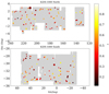Fig. 1. KiDS North and South survey areas are shown in light grey in the upper and lower panels, respectively. The positions of ACT clusters used in this analysis are indicated by each circle. The colour of the circles corresponds to cluster redshift, with yellow indicating high redshift and black indicating low redshift. The size of each circle scales with the SZ signal-to-noise, which is correlated with the cluster mass when the noise is the same everywhere, such that larger circles represent clusters with a greater SZ signal-to-noise than smaller circles.

Hilton et al. (2021) estimate the Compton–y parameter and associated SZ mass, M_SZ, for each cluster; we summarise their method here. The signal we observe, at a projected angle θ from the cluster centre, due to the SZ effect is a change in radiation intensity which can be expressed in terms of CMB temperature by

$$\begin{array}{c}\hfill \frac{\mathrm{\Delta }T(\theta )}{T_{\mathrm{CMB}}}=f_{\mathrm{SZ}}y(\theta ),\end{array}$$(2)

where y(θ) is the line-of-sight integrated pressure profile. In the non-relativistic limit, f_SZ only depends on the observed radiation frequency. In Hilton et al. (2021) a correction factor f_rel is applied to include relativistic effects for gas temperature, as determined in Itoh et al. (1998).

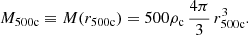
The Compton–y signal is modelled using the universal pressure profile (Arnaud et al. 2010) which describes the intra-cluster gas pressure, p, as a function of scaled radius, x = r/r_500c where r_500c is the radius within which the density is 500 times the critical density ρ_c, at z = 0. This relation was modelled with a generalised Navarro-Frenk-White (NFW) profile from Nagai (2006) as

$$\begin{array}{c}\hfill p(x)=\frac{p_0}{{(c_{500}x)}^{\gamma }{[1+{(c_{500}x)}^{\alpha }]}^{(\beta -\gamma )/\alpha }},\end{array}$$(3)

where c₅₀₀ is the concentration parameter and {γ, α, β} describe the slope at different radii. This includes any mass dependence in the profile shape and has been calibrated to X-ray observations of nearby clusters.

Hilton et al. (2021) combine Eqs. (2) and (3) to produce a frequency-dependent matched filter across a range of masses and redshifts (each of which change the amplitude and width of the filter). Following Arnaud et al. (2010), the matched filter amplitude, ${\stackrel{\sim }{\mathit{y}}}_0$, can be related to cluster mass via

$$\begin{array}{c}\hfill {\stackrel{\sim }{y}}_0={10}^{A_0}{E}^2(z){\left(\frac{M_{\mathrm{SZ},500}}{M_{\mathrm{piv}}}\right)}^{1+B_0}Q(M_{\mathrm{SZ},500},z)f_{\mathrm{rel}}(M_{\mathrm{SZ},500},z),\end{array}$$(4)

where 10^A₀ = 4.95  ×  10⁻⁵ is the normalisation, E(z) is the ratio of the Hubble constant at a redshift z to the present value, B₀ = 0.08 is a scaling parameter and M_piv = 3 × 10¹⁴ M_⊙ is a mass normalisation parameter. The cluster-filter scale mismatch function Q accounts for the discrepancy between the size of a cluster with a different mass and redshift to the reference model used to define the matched filter, which includes the effects of the beam (see Hasselfield et al. 2013, for full details). The location of the cluster is then defined as the peak of the SZ signal. An alternative definition of the cluster centre is the brightest cluster galaxy (BCG) which is expected to be a better tracer of the true centre compared to the SZ signal which is tracing the gas distribution. This is investigated further in Appendix A however in our main analysis we take the BCG as the cluster centre.

To obtain the cluster mass, the intrinsic scatter σ_c in the y − M scaling relation must be accounted for. Hilton et al. (2021) assume a log-normal distribution with dispersion σ_c = 0.2. This level of scatter is consistent with both numerical simulations (Bode et al. 2012) and dynamical mass measurements of clusters (Sifón et al. 2013). The distribution of SZ derived cluster masses (M_SZ) for our sample is shown in the lower panel of Fig. 2. We note that the values of M_SZ used in this analysis have no prior (1 − b_SZ) correction applied.

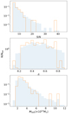Fig. 2. Upper: normalised SZ signal-to-noise distribution of the ACT clusters found in the KiDS-1000 region. Middle: normalised redshift distribution of these clusters. Lower: normalised SZ-derived mass distribution of these clusters, estimated from the SZ observable Compton–y values. The blue shaded region corresponds to clusters selected to have an SZ signal-to-noise greater than 5 and in the redshift range 0.1–0.9 across the full ACT footprint. The orange line corresponds to the selection of 157 clusters used in this analysis that lie within the KiDS footprint.

2.2. Weak Gravitational Lensing from the Kilo Degree Survey

KiDS is an optical survey utilising the OmegaCAM CCD mosaic camera on the VLT Survey Telescope in Chile (de Jong et al. 2015). For this analysis we are using the most recent KiDS dataset, KiDS-1000, first presented in Kuijken et al. (2019)². This catalogue includes 30 million galaxies across two areas of sky based around the GAMA spectroscopic survey. KiDS-1000 was observed in 4 bands, {u, g, r, i} with an additional five bands {Z, Y, J, H, K_s} observed by the VISTA Kilo-Degree Infrared Galaxy survey (VIKING; Edge et al. 2013), making KiDS a deep and wide nine-band imaging dataset (Wright et al. 2019). KiDS-1000 includes 1006 deg² of imaging with galaxy lensing measurements and accurately calibrated photometric redshifts to z_B < 1.2 (Wright et al. 2020). The redshift distributions we use in this analysis are calibrated following the methods adopted in the KiDS-1000 cosmology analyses (Asgari et al. 2021; Heymans et al. 2021) which use a self-organising map (SOM). This approach removes source galaxies from our sample because their redshift could not be accurately calibrated with spectroscopic datasets, resulting from incompleteness in the spectroscopic sample (Wright et al. 2020; Hildebrandt et al. 2021). We select source galaxies by their photometric redshift estimate, z_B, which is derived from the nine-band imaging using the Bayesian Photometric Redshifts code (BPZ; Benítez 2000). For each cluster lensing measurement, source galaxies are selected to have z_B > z_l + 0.2, where z_l is the redshift of the lens. This selection aims to eliminate unlensed galaxies from our source galaxy sample, although correction factors are still required (discussed in Sect. 2.3). A redshift distribution calibrated by the SOM, based on this z_B redshift selection, is produced for each cluster. The more selective nature of the SOM method has reduced the galaxy number density and therefore increased the statistical error over the same area, however, the systematic error associated with the photometric redshift distribution has decreased. Source galaxy shape measurements are computed with the lensfit pipeline (Miller et al. 2013), which is calibrated with simulations described in Kannawadi et al. (2019) and presented in Giblin et al. (2021). KiDS-1000 has an effective number density of 6.17 arcmin⁻², in the photometric redshift range (0.1 < z_B < 1.2), and the variance of the ellipticities is on average 0.265 (see Table 1, Giblin et al. 2021). For more technical details on the survey see Kuijken et al. (2019). The footprint of the observed KiDS region is shown in Fig. 1.

2.3. The excess surface density

We summarise the formalism for estimating the weak gravitational lensing signal around a stack of clusters, following Bartelmann & Schneider (2001). Considering an isolated cluster, weak lensing introduces a systematic tangential alignment of the images of the source galaxies relative to the lens. We use the average tangential distortion, γ_t, to quantify the lensing signal. This is calculated from the two components of shear, [γ₁, γ₂],

$$\begin{array}{c}\hfill \left(\begin{array}{c}{\gamma }_{\mathrm{t}}\\ {\gamma }_{\times }\\ \end{array}\right)=\left(\begin{array}{cc}-cos2\varphi & -sin2\varphi \\ sin2\varphi & -cos2\varphi \\ \end{array}\right)\left(\begin{array}{c}{\gamma }_1\\ {\gamma }_2\\ \end{array}\right),\end{array}$$(5)

where, in a flat sky approximation, ϕ is the angle measured from a line of constant declination to a given source galaxy relative to the centre of the lens and γ_× is the shear component along the 45° rotated direction. In practice, γ_t and γ_× are both averaged over all angles so that a gravitational lensing signal can be detected from the average γ_t, and the average γ_× is a useful control statistic that should be consistent with zero for a signal solely caused by gravitational lensing.

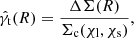
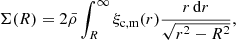
Since the tangential distortion we observe is due to intervening matter along the line of sight, the average γ_t of source galaxies, at a projected comoving separation R from the cluster lens can be expressed in terms of the excess surface density, ΔΣ,

$$\begin{array}{c}\hfill {\widehat{\gamma }}_{\mathrm{t}}(R)=\frac{\mathrm{\Delta }\mathrm{\Sigma }(R)}{{\mathrm{\Sigma }}_{\mathrm{c}}({\chi }_{\mathrm{l}},{\chi }_{\mathrm{s}})},\end{array}$$(6)

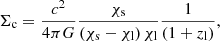
where Σ_c is the comoving critical surface density, written in terms of comoving distances, given by

$$\begin{array}{c}\hfill {\mathrm{\Sigma }}_{\mathrm{c}}=\frac{c^2}{4\pi G}\frac{{\chi }_{\mathrm{s}}}{({\chi }_{\mathrm{s}}-{\chi }_{\mathrm{l}}){\chi }_{\mathrm{l}}}\frac{1}{(1+z_{\mathrm{l}})},\end{array}$$(7)

for spatially flat models only and χ is the comoving distance to the lens χ_l and the source χ_s and z_l is the lens redshift. The excess surface density (ESD) is defined as

$$\begin{array}{c}\hfill \mathrm{\Delta }\mathrm{\Sigma }(R)\equiv \overline{\mathrm{\Sigma }}(<R)-\mathrm{\Sigma }(R),\end{array}$$(8)

with the average mass density within a radius R given by

$$\begin{array}{c}\hfill \overline{\mathrm{\Sigma }}(<R)\equiv \frac{2}{R^2}{\displaystyle {\int }_0^R}{R}^{\prime }\mathrm{\Sigma }(R^{\prime })\mathrm{d}{R}^{\prime }.\end{array}$$(9)

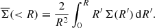
Equation (6) can be generalised for broad lens and source redshift distributions, n_l and n_s to give

$$\begin{array}{c}\hfill ⟨{\gamma }_{\mathrm{t}}⟩(R)={\displaystyle {\int }_0^{\infty }\mathrm{d}z{n}_{\mathrm{l}}(z)\mathrm{\Delta }\mathrm{\Sigma }(R,z){\int }_z^{\infty }\mathrm{d}{z}^{\prime }{n}_{\mathrm{s}}(z^{\prime })\frac{1}{{\mathrm{\Sigma }}_{\mathrm{c}}(z,z^{\prime })}·}\end{array}$$(10)

For a narrow lens and source redshift distribution, n_l(z) = δ_D(z − z_l) and n_s(z′) = δ_D(z′−z_s), so that the above equation reduces to Eq. (6). Equation (10) cannot be solved for in closed form, but for a narrow lens redshift distribution, averaging over a background source redshift distribution, n(z_s), we find

$$\begin{array}{c}\hfill \mathrm{\Delta }\mathrm{\Sigma }(R,z_{\mathrm{l}})\approx ⟨{\gamma }_{\mathrm{t}}⟩(R){{\displaystyle \left[{\int }_{z_{\mathrm{l}}}^{\infty }\mathrm{d}{z}_{\mathrm{s}}n(z_{\mathrm{s}})\frac{1}{{\mathrm{\Sigma }}_{\mathrm{c}}(z_{\mathrm{l}},z_{\mathrm{s}})}\right]}}^{-1}·\end{array}$$(11)

This equation can be re-written as

$$\begin{array}{c}\hfill \mathrm{\Delta }\mathrm{\Sigma }(R,z_{\mathrm{l}})=\frac{⟨{\gamma }_{\mathrm{t}}⟩(R)}{\overline{{\mathrm{\Sigma }}_{\mathrm{c}}^{-1}}},\end{array}$$(12)

where, for a given dataset, the average inverse critical surface density, $\overline{{\mathrm{\Sigma }}_c^{-1}}$, is defined as

$$\begin{array}{cc}\hfill \overline{{\mathrm{\Sigma }}_{\mathrm{c},\mathrm{l}}^{-1}}& \equiv {\displaystyle {\int }_{z_{\mathrm{l}}}^{\infty }}\mathrm{d}{z}_{\mathrm{s}}n(z_{\mathrm{s}}){\mathrm{\Sigma }}_{\mathrm{c}}^{-1}(z_{\mathrm{l}},z_{\mathrm{s}})\hfill \\ \hfill & =\frac{4\pi G}{c^2}(1+z_{\mathrm{l}}){\chi }_{\mathrm{l}}{\displaystyle {\int }_{z_{\mathrm{l}}}^{\infty }\mathrm{d}{z}_{\mathrm{s}}n(z_{\mathrm{s}})(1-\frac{{\chi }_{\mathrm{l}}}{{\chi }_{\mathrm{s}}})·}\hfill \end{array}$$(13)

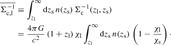
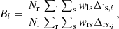
From the equations derived above we can write an estimator for the ESD as

$$\begin{array}{c}\hfill \mathrm{\Delta }{\mathrm{\Sigma }}_i=\frac{{\sum }_{\mathrm{l}}{\sum }_{\mathrm{s}}{w}_{\mathrm{ls}}{ϵ}_{\mathrm{t},\mathrm{s}}{\left(\overline{{\mathrm{\Sigma }}_{\mathrm{c},\mathrm{l}}^{-1}}\right)}^{-1}{\mathrm{\Delta }}_{\mathrm{ls},i}}{{\sum }_{\mathrm{l}}{\sum }_{\mathrm{s}}{w}_{\mathrm{ls}}{\mathrm{\Delta }}_{\mathrm{ls},i}},\end{array}$$(14)

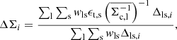
where Δ_ls,i is a bin selector function which is defined to be unity if the radial separation between a foreground lens l and background source s, lies within a bin centred on R_i. The tangential ellipticity of source galaxy s projected on to an axis perpendicular to the line between the lens and source is given by ϵ_t, s and the weight, w_ls assigned to a given source galaxy, s, behind a lens, l, is

$$\begin{array}{c}\hfill w_{\mathrm{ls}}=w_{\mathrm{s}}{\left(\overline{{\mathrm{\Sigma }}_{\mathrm{c},\mathrm{l}}^{-1}}\right)}^2.\end{array}$$(15)

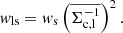
Since our shape measurement pipeline uses lensfit, each source galaxy has a corresponding weight which is approximately an inverse variance weighting that accounts for total shape noise, 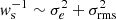$w_{\mathrm{s}}^{-1}\sim {\sigma }_e^2+{\sigma }_{\mathrm{rms}}^2$, where σ_rms is the intrinsic shape dispersion, and σ_e is the shape measurement error.

Due to the uncertainty associated with the photometric redshifts of the source galaxies, there will be some source galaxies that are a cluster member or a foreground galaxy. This leads to a dilution of the lensing signal and therefore a mass estimate that is biased low. This effect can be corrected for by making the same ESD measurements around 100 random positions, denoted with the subscript r, that are unclustered but still have the same selection function as the lensing clusters. This approach was first shown for the tangential shear estimator (Mandelbaum et al. 2006) but can analogously be applied to the ESD (Singh et al. 2017) as

$$\begin{array}{c}\hfill \mathrm{\Delta }{\mathrm{\Sigma }}_i=\frac{{\sum }_{\mathrm{l}}{\sum }_{\mathrm{s}}{w}_{\mathrm{ls}}{ϵ}_{\mathrm{t},\mathrm{ls}}{\left(\overline{{\mathrm{\Sigma }}_{\mathrm{c},\mathrm{l}}^{-1}}\right)}^{-1}{\mathrm{\Delta }}_{\mathrm{ls},i}}{{\sum }_{\mathrm{r}}{\sum }_{\mathrm{s}}{w}_{\mathrm{rs}}{\mathrm{\Delta }}_{\mathrm{rs},i}}\left(\frac{N_{\mathrm{r}}}{N_{\mathrm{l}}}\right)-\frac{{\sum }_{\mathrm{r}}{\sum }_{\mathrm{s}}{w}_{\mathrm{rs}}{ϵ}_{\mathrm{t},\mathrm{rs}}\left(\overline{{\mathrm{\Sigma }}_{\mathrm{c},\mathrm{r}}^{-1}}\right){\mathrm{\Delta }}_{\mathrm{rs},i}}{{\sum }_{\mathrm{r}}{\sum }_{\mathrm{s}}{w}_{\mathrm{rs}}{\mathrm{\Delta }}_{\mathrm{rs},i}}·\end{array}$$(16)

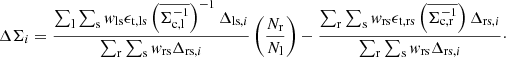
Here N_l and N_r are the number of lenses and random positions respectively within radial bin Δ_ls,i. Normalising with random lenses produces an unbiased estimate of the ESD unaffected by any source-lens clustering, compared to Eq. (14). This is often referred to as the “boost” factor (Sheldon et al. 2004) which is given by

$$\begin{array}{c}\hfill B_i=\frac{N_{\mathrm{r}}}{N_{\mathrm{l}}}\frac{{\sum }_{\mathrm{l}}{\sum }_{\mathrm{s}}{w}_{\mathrm{ls}}{\mathrm{\Delta }}_{\mathrm{ls},i}}{{\sum }_{\mathrm{r}}{\sum }_{\mathrm{s}}{w}_{\mathrm{rs}}{\mathrm{\Delta }}_{{\mathrm{rs},}_i}},\end{array}$$(17)

for the case of lenses and random positions having no additional weighting applied. In our analysis we ensure our random sample has the same area and redshift properties as our cluster sample.

We apply an additional correction factor to account for multiplicative bias shear calibration which accounts for uncertainty in the shape measurement calibration (Kannawadi et al. 2019) and multiplies the ESD estimator defined in Eq. (16) as $\frac{1}{(1+{\overline{m}}_i)}\mathrm{\Delta }{\mathrm{\Sigma }}_i$ for

$$\begin{array}{c}\hfill {\overline{m}}_i=\frac{{\sum }_{\mathrm{l}}{\sum }_{\mathrm{s}}{w}_{\mathrm{ls}}{m}_{\mathrm{s}}{\mathrm{\Delta }}_{ls,i}}{{\sum }_{\mathrm{l}}{\sum }_{\mathrm{s}}{w}_{\mathrm{ls}}{\mathrm{\Delta }}_{ls,i}}·\end{array}$$(18)

Here m_s is given by the multiplicative bias value of the tomographic bin which the source s falls into based on its z_B value. The value of the multiplicative bias per tomographic bin are described in Asgari et al. (2021) and were determined in Kannawadi et al. (2019).

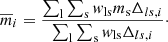
For the stacked ESD measurement we estimate the covariance matrix following the same procedure as Miyatake et al. (2019) as

$$\begin{array}{c}\hfill \mathsf{C}={\mathsf{C}}^{\mathrm{stat}}+{\mathsf{C}}^{\mathrm{lss}}+{\mathsf{C}}^{\mathrm{int}},\end{array}$$(19)

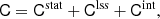
where C^stat accounts for the statistical uncertainty due to galaxy shapes, C^lss is the covariance due to projection effects from uncorrelated large-scale structure (Hoekstra 2001) and C^int corresponds to the intrinsic variations due to halo triaxiality and correlated halos. The contribution to the covariance from shape noise is diagonal by definition and is given by

$$\begin{array}{c}\hfill {\sigma }_{\mathrm{stat},i}^2={\sigma }_e^2[\frac{{\sum }_{\mathrm{ls}}{\left(w_{\mathrm{ls}}\overline{{\mathrm{\Sigma }}_{\mathrm{c},\mathrm{l}}^{-1}}\right)}^2{\mathrm{\Delta }}_{\mathrm{ls},i}}{{\left({\sum }_{\mathrm{rs}}{w}_{\mathrm{rs}}{\overline{{\mathrm{\Sigma }}_{\mathrm{c},\mathrm{r}}^{-1}}}^2{\mathrm{\Delta }}_{\mathrm{rs},i}\right)}^2}{\left(\frac{N_{\mathrm{r}}}{N_{\mathrm{l}}}\right)}^2+\frac{{\sum }_{\mathrm{rs}}{\left(w_{\mathrm{ls}}\overline{{\mathrm{\Sigma }}_{\mathrm{c},\mathrm{l}}^{-1}}\right)}^2{\mathrm{\Delta }}_{\mathrm{rs},i}}{{\left({\sum }_{\mathrm{rs}}{w}_{\mathrm{rs}}{\overline{{\mathrm{\Sigma }}_{\mathrm{c},\mathrm{r}}^{-1}}}^2{\mathrm{\Delta }}_{\mathrm{rs},i}\right)}^2}],\end{array}$$(20)

for the estimator given in Eq. (16). The large-scale structure and intrinsic parts of the covariance are defined in Eqs. (A.1) and (A.7) in Miyatake et al. (2019).

3. Results

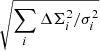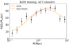In our fiducial analysis we measure the ESD, ΔΣ, “stacking” all 157 ACT-detected clusters, as given by Eq. (14). The lensing signal is detected with a signal-to-noise of 25 in the range 0.1–10 Mpc from the cluster centres, and the ESD profile is shown in Fig. 3. The detection significance is computed as $\sqrt{\sum _i\mathrm{\Delta }{\mathrm{\Sigma }}_i^2/{\sigma }_i^2}$.

Fig. 3. ESD profile (ΔΣ) multiplied by the radius R as a function of radius R for the complete stack of 157 SZ-detected clusters. The signal is detected at 25σ significance. The best-fitting model is shown using a single NFW, shown in red, and the halo model, shown in orange. A limited range of scales is used for the NFW model to avoid the impact of mis-centring at small scales and the contribution from large-scale structure at scales greater than 5 Mpc. Both models give good fits to the data.

3.1. Modelling the stacked ESD

We estimate the weak lensing mass, M_WL, of the stacked clusters using two models: a single NFW halo (Navarro et al. 1997) and a full halo model (Peacock & Smith 2000; Seljak 2000). The single NFW fit assumes that the measured lensing signal is only due to the cluster. The halo model also assumes that the central cluster halo is described by an NFW but additionally accounts for line-of-sight lensing. Furthermore, the halo model method is superior for modelling the ESD signal, as the ACT selection function can be included and we also use a modified NFW profile to account for mis-centring at small scales. We include the NFW fit to compare our results with previous analyses which have utilised a similar modelling approach.

The signal we observe is actually the reduced shear g = γ/(1 − κ), where κ is the convergence which accounts for the change in size of an object due to gravitational lensing. At large scales κ is very small and so the true shear, γ ≈ g. At small scales, however, κ is larger and the equivalence of g and γ no longer holds. Given that we use data at small scales, we apply a correction to our model for the ESD signal to account for reduced shear following Schrabback et al. (2018).

This factor simply multiplies the model for the ESD as f_reduce ΔΣ^model and is given for a stack of clusters as

$$\begin{array}{c}\hfill f_{\mathrm{reduce}}=[1+(\frac{⟨{\beta }_s^2⟩}{{⟨{\beta }_s⟩}^2}-1)⟨{\beta }_s⟩{\kappa }_{\infty }^{\mathrm{model}}]\frac{1}{(1-⟨{\beta }_s⟩{\kappa }_{\infty }^{\mathrm{model}})},\end{array}$$(21)

where ${\kappa }_{\infty }^{\mathrm{model}}$ is the model convergence computed at infinite redshift and the shape weights are accounted for as

$$\begin{array}{c}\hfill ⟨{\beta }_s⟩=\frac{\sum {\beta }_{\mathrm{l}}{w}_{\mathrm{l}}}{\sum w_{\mathrm{l}}},⟨{\beta }_s^2⟩=\frac{\sum {\beta }_{\mathrm{l}}^2{w}_{\mathrm{l}}}{\sum w_{\mathrm{l}}},\end{array}$$(22)

where β_l is computed per lens for the estimated source redshift distribution as

$$\begin{array}{c}\hfill {\beta }_{\mathrm{l}}=\frac{{\chi }_{\infty }}{({\chi }_{\infty }-{\chi }_{\mathrm{l}})}{\displaystyle {\int }_{z_{\mathrm{l}}}^{\infty }}\mathrm{d}{z}_{\mathrm{s}}n(z_{\mathrm{s}})\frac{({\chi }_{\mathrm{s}}-{\chi }_{\mathrm{l}})}{{\chi }_{\mathrm{s}}}·\end{array}$$(23)

The $\frac{⟨{\beta }_s^2⟩}{{⟨{\beta }_s⟩}^2}$ in the correction term accounts for the width in the redshift distribution (Applegate et al. 2014; Hoekstra et al. 2000; Seitz & Schneider 1997). For our sample this correction factor is ∼1.3 at the smallest scales, which correspond to 1σ shift in the ESD. For R > 0.5 Mpc the correction factor decreases to less than 1.05.

3.1.1. Single NFW

We estimate the average cluster mass, M_WL, by assuming an NFW density profile (Navarro et al. 1997) and calculating the expected ESD using Wright & Brainerd (2000), summarised here. The NFW profile is given by

$$\begin{array}{c}\hfill \rho (r)=\frac{{\delta }_c{\rho }_{\mathrm{c}}}{(r/r_{\mathrm{s}}){(1+r/r_{\mathrm{s}})}^2},\end{array}$$(24)

where the characteristic overdensity, δ_c, is related to the NFW concentration parameter, c₅₀₀ via

$$\begin{array}{c}\hfill {\delta }_c=\frac{500}{3}\frac{c_{500}^3}{[ln(1+c_{500})-c_{500}/(1+c_{500})]}·\end{array}$$(25)

In Eq. (24), r_s = r_500c/c₅₀₀ is the scale radius. We use the r_500c radius to be consistent with the SZ measurements which also use this definition. The mass within a radius of r_500c, is given by

$$\begin{array}{c}\hfill M_{500\mathrm{c}}\equiv M(r_{500\mathrm{c}})=500{\rho }_{\mathrm{c}}\frac{4\pi }{3}{r}_{500\mathrm{c}}^3.\end{array}$$(26)

Within this model we fit the mass, $M_{500\mathrm{c}}^{\mathrm{WL}}$, and the concentration, c₅₀₀, using wide flat priors and take the average cluster redshift of z = 0.36, which is calculated by weighting the clusters using the weights defined in Eq. (15). Fitting for the concentration, rather than assuming a mass-concentration relation which has been calibrated on dark matter-only simulations, has been shown to capture the change in the ESD profile due to baryon feedback which effectively redistributes material from the centre to the outer regions of the cluster. Debackere et al. (2021) showed that when assuming a mass-concentration relation, the mass inferred from weak lensing can be overestimated by 10% at the smallest scales and underestimated by around 5% at the largest scales considered in our analysis. Allowing the concentration and mass to vary removes the bias at large scales and reduces the bias at small scales to less than 5% for the largest halos, which are most affected, and to ∼1% for the halos with a mass comparable to those considered in this work. Thus this approach for mitigating the impact of baryons is sufficient in decreasing the bias in the mass estimate. Debackere et al. (2021) demonstrated however that when performing a cosmological analysis the bias in cosmological parameters increases due to a mis-match in the mass definition when the mass function is obtained from dark matter-only simulations. As a result the inferred bias cannot be directly applied as a calibration in a cosmological analysis. Similar arguments have been put forward by Cromer et al. (2022), who implemented a generalised NFW – which allows for a more flexible radial dependence of the density profile – to account for the effects of baryons, and found biases 5–10% when adopting an NFW profile. We therefore caution against over interpreting c; it should not be thought of as the concentration of an underlying NFW model but as a catch-all for a variety of effects that may modify the inner mass profiles of clusters.

The best-fitting NFW model is shown in Fig. 3, which has a p-value of 0.81. We only use the range (0.5 < R < 5) Mpc to avoid any mis-centring biases at small scales (see Appendix A), and to avoid including the potentially significant signal from the large-scale structure at scales greater than 5 Mpc (Applegate et al. 2014). This upper limit was chosen apriori and the lower limit was informed by the analysis presented in Appendix A although this is consistent with the ranges used in previous cluster weak lensing analyses. We compute the average weak lensing mass to be $M_{500\mathrm{c}}^{\mathrm{NFW}}=(4.9\pm 0.4)\times {10}^{14}{M}_{\odot }$.

3.1.2. Halo model method

Cluster lensing can be understood within the framework of the halo model following Seljak (2000), Peacock & Smith (2000), Cooray & Sheth (2002). The projected surface density is completely specified by the cluster–matter cross correlation, ξ_c, m, which can be computed from a given halo occupation model,

$$\begin{array}{c}\hfill \mathrm{\Sigma }(R)=2\overline{\rho }{\displaystyle {\int }_R^{\infty }}{\xi }_{\mathrm{c},\mathrm{m}}(r)\frac{r\mathrm{d}r}{\sqrt{r^2-R^2}},\end{array}$$(27)

where r is the 3D comoving distance r² = R² + (χ − χ_l)², for a flat Universe. The cluster–matter cross correlation power spectrum, at a wavenumber k, is given in terms of ξ_c, m as

$$\begin{array}{c}\hfill P_{\mathrm{c},\mathrm{m}}(k)=4\pi {\displaystyle {\int }_0^{\infty }}{\xi }_{\mathrm{c},\mathrm{m}}(r)\frac{sin(kr)}{\mathit{kr}}{r}^2\mathrm{d}r.\end{array}$$(28)

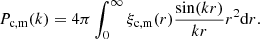
The power spectrum of the cluster–dark matter cross correlation can be split into two parts:

$$\begin{array}{c}\hfill P_{\mathrm{c},\mathrm{m}}(k)=P_{\mathrm{c},\mathrm{m}}^{1\mathrm{h}}(k)+P_{\mathrm{c},\mathrm{m}}^{2\mathrm{h}}(k),\end{array}$$(29)

with the 1-halo term, which includes the non-linear regime at small scales, and the 2-halo term which describes the clustering between halos, which is dominant on large scales.

The 1-halo term, $P_{\mathrm{c},\mathrm{m}}^{1\mathrm{h}}(k)$, describes the matter distribution inside halos hosting clusters. For a single cluster, this is

$$\begin{array}{c}\hfill P_{\mathrm{c},\mathrm{m}}^{1\mathrm{h}}(k)=\frac{1}{\overline{\rho }}{u}_{\mathrm{c}}(k|M),\end{array}$$(30)

where u_c(k|M) is the Fourier transform of the cluster density profile ρ(r|M), which we assume to be described by an NFW profile.

Since we are measuring a stack of clusters, the 1-halo term becomes

$$\begin{array}{c}\hfill P_{\mathrm{c},\mathrm{m}}^{1\mathrm{h}}(k)=\frac{1}{\overline{\rho }}{\displaystyle {\int }_0^{\infty }}\mathcal{P}(M)u_{\mathrm{c}}(k|M)\mathrm{d}M,\end{array}$$(31)

where 𝒫(M) is the probability that a cluster within an SZ sample resides in a halo of mass M, which is given

$$\begin{array}{c}\hfill \mathcal{P}(M)\mathrm{d}M=\frac{\langle N_{\mathrm{c}}|M\rangle \frac{\mathrm{d}n(M)}{\mathrm{d}M}}{{\overline{n}}_{\mathrm{c}}}\mathrm{d}M,\end{array}$$(32)

where ⟨N_c|M⟩ is the average number of clusters in the SZ selection with a halo of mass M, $\frac{\mathrm{d}n(M)}{\mathrm{d}M}$ is the halo mass function and 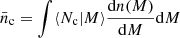${\overline{n}}_{\mathrm{c}}=\int ⟨N_{\mathrm{c}}|M⟩\frac{\mathrm{d}n(M)}{\mathrm{d}M}\mathrm{d}M$ is the comoving number density of clusters in the SZ selection. Equation (31) can therefore be re-written as:

$$\begin{array}{c}\hfill P_{\mathrm{c},\mathrm{m}}^{1\mathrm{h}}(k)=\frac{1}{\overline{\rho }{\overline{n}}_{\mathrm{c}}}{\displaystyle {\int }_0^{\infty }}\mathrm{d}M\frac{\mathrm{d}n(M)}{\mathrm{d}M}{u}_{\mathrm{c}}(k|M)⟨N_{\mathrm{c}}|M⟩.\end{array}$$(33)

This 1-halo term is constructed so that mis-centring of clusters can be accounted for in the cluster density profile, via the u_c(k|M) term defined as

$$\begin{array}{c}\hfill u_{\mathrm{c}}(k|M)=u_{\mathrm{dm}}(k|M)(1-p_{\mathrm{off}}+p_{\mathrm{off}}{e}^{-0.5k^2{(r_{\mathrm{s}}{f}_{\mathrm{off}})}^2}),\end{array}$$(34)

where, p_off and f_off is the probability of mis-centring and the size of the offset, as fraction of r_s, respectively.

The 2-halo term, denoted by $P_{\mathrm{c},\mathrm{m}}^{2\mathrm{h}}(k)$, describes the correlation between clusters and dark matter particles belonging to separate haloes, and is given by

$$\begin{array}{cc}\hfill P_{\mathrm{c},\mathrm{m}}^{2\mathrm{h}}(k)& =\frac{P_{\mathrm{dm}}(k)}{\overline{\rho }}{\displaystyle {\int }_0^{\infty }}\mathcal{P}(M)b_{\mathrm{h}}(M)\mathrm{d}M\hfill \\ \hfill & {\displaystyle {\int }_0^{\infty }{u}_{\mathrm{dm}}(k|M^{\prime })b_{\mathrm{h}}(M^{\prime })\frac{\mathrm{d}n(M^{\prime })}{\mathrm{d}{M}^{\prime }}\mathrm{d}{M}^{\prime }.}\hfill \end{array}$$(35)

Here P_dm is the matter power spectrum, which we assume to be linear, and b_h(M) is the halo bias function. The halo bias function describes how halos of mass M are biased with respect to the overall dark matter distribution. Using Eq. (32), we can re-write Eq. (35) as

$$\begin{array}{cc}\hfill P_{\mathrm{c},\mathrm{m}}^{2\mathrm{h}}(k)& =\frac{P_{\mathrm{dm}}(k)}{\overline{\rho }{\overline{n}}_{\mathrm{c}}}{\displaystyle {\int }_0^{\infty }}⟨N_{\mathrm{c}}|M⟩b(M)\frac{\mathrm{d}n(M)}{\mathrm{d}M}\mathrm{d}M\hfill \\ \hfill & {\displaystyle {\int }_0^{\infty }{u}_{\mathrm{dm}}(k|M^{\prime })b(M^{\prime })\frac{\mathrm{d}n(M^{\prime })}{\mathrm{d}{M}^{\prime }}\mathrm{d}{M}^{\prime }.}\hfill \end{array}$$(36)

We adopt the halo bias model from Tinker et al. (2010) and include an amplitude A_b that multiplies the halo bias as b(M) = A_bb_h(M), which we marginalise over in our halo model analysis. For the halo occupation statistics that are required to calculate ⟨N_c|M⟩, we assume a simple power-law dependence between halo mass M and M_SZ

$$\begin{array}{c}\hfill M_{\mathrm{SZ}}=A{M}^{\beta },\end{array}$$(37)

to calculate the average number of clusters. Given the limited signal-to-noise ratio of the data we fix the mass-dependent exponent, β, equal to 1, so that we can focus on A, which quantifies the constant mass bias between the SZ mass and the true mass. This assumption is justified by the fact that there is no significant evidence for a mass dependence of the SZ bias when combining studies probing different cluster masses (see Fig. 4). For our sample of clusters, the average number of clusters is then given by,

$$\begin{array}{c}\hfill ⟨N_c|M⟩=\frac{1}{\sqrt{2\pi }{\sigma }_c}{\displaystyle {\int }_0^{\infty }}\frac{S(M_{\mathrm{SZ}})}{M_{\mathrm{SZ}}}{\mathrm{e}}^{\left[\frac{-{(ln(M_{\mathrm{SZ}}/M)-lnA)}^2}{2{\sigma }_c^2}\right]}\mathrm{d}{M}_{\mathrm{SZ}},\end{array}$$(38)

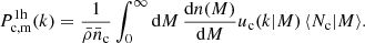
Fig. 4. Estimated (1 − bSZ) bias parameter from this analysis (ACT SZ-detected clusters calibrated with KiDS weak lensing), compared to other recent results. Shown on this figure at the lower mass range, the analyses of ACT and Planck clusters using HSC (Miyatake et al. 2019; Medezinski et al. 2018), ACT/CS82 (Battaglia et al. 2016), CLASH (Penna-Lima et al. 2017), PSZ2LenS (Sereno et al. 2017), WtG (von der Linden et al. 2014), CCCP (Hoekstra et al. 2015) which has recently been updated to CCCP and MENeaCS (Herbonnet et al. 2020) and Planck clusters with Planck CMB lensing (Zubeldia & Challinor 2019) analyses. The blue band indicates the prediction from Planck primary CMB measurements if the ΛCDM model is correct (Planck Collaboration VI 2020), given the SZ clusters observed by Planck. This value is computed using a Planck Collaboration VI (2020) primary CMB best fit cosmology, however using the cosmology derived from ACT DR6 lensing, Madhavacheril et al. (2023), would give the same result.

where we have assumed a log-normal scatter, σ_c, and S(M_SZ) is the SZ-experiment selection function, which can be computed for a given range in SZ signal-to-noise. We fix the SZ mass scatter to σ_c = 0.2, firstly because lensing does not constrain this well and secondly because this is the same scatter taken to correct the Eddington bias selection effect for the SZ masses derived for the ACT clusters (Hilton et al. 2021), based on the level of scatter seen in numerical simulations and dynamical mass measurements. We check that the chosen value for the scatter does not significantly impact our estimate of (1 − b_SZ) by repeating our analysis with σ_c = 0.001 and σ_c = 0.5. Our inferred value for the mass changes by less than 0.2σ which has a 2% effect on (1 − b_SZ).

In this model we fit for the following set of parameters: {c, lnA, A_b, p_off, f_off}. The average halo mass, which is the main parameter we are interested in, is a derived parameter, given by

$$\begin{array}{c}\hfill M_{500\mathrm{c}}^{\mathrm{HM}}\equiv M_{\mathrm{h}}=\frac{1}{{\overline{n}}_{\mathrm{c}}}{\displaystyle \int }⟨N_{\mathrm{c}}|M⟩M\frac{\mathrm{d}n(M)}{\mathrm{d}M}\mathrm{d}M.\end{array}$$(39)

Our halo model framework described above is built from the halo model modules in the public Core Cosmology Library (Chisari et al. 2019).

We use Bayesian inference to recover the posterior probability distribution of these five parameters using EMCEE, the MCMC Python package (Foreman-Mackey et al. 2013). We use wide flat priors for all parameters (c ∈ [0, 10], lnA ∈ [ − 5, 5], A_b ∈ [0, 10], p_off ∈ [0, 1], f_off ∈ [0, 1]) and assume a Gaussian likelihood given by

$$\begin{array}{cc}\hfill ln\mathcal{L}& [\mathrm{\Delta }{\mathrm{\Sigma }}_{\mathrm{obs}}(R)|\mathrm{\Delta }\mathrm{\Sigma }(R,q)]=\hfill \\ \hfill & -\frac{1}{2}(\mathrm{\Delta }{\mathrm{\Sigma }}_{\mathrm{obs}}(R)-\mathrm{\Delta }\mathrm{\Sigma }(R,q){)}^T{\mathsf{C}}_{R,R^{\prime }}^{-1}(\mathrm{\Delta }{\mathrm{\Sigma }}_{\mathrm{obs}}(R)-\mathrm{\Delta }\mathrm{\Sigma }(R,q)),\hfill \end{array}$$(40)

for the set of parameters q. We note that since the effective concentration and halo bias parameters are nuisance parameters, which do not have a significant impact on the posterior distribution, sampling in linear or log space has no impact on our results. We fix the cosmological parameters to Planck Collaboration VI (2020), which are in excellent agreement with the recent CMB lensing results from ACT (Madhavacheril et al. 2023), for computing P_dm. Assuming a value for σ₈ which has been determined at a similar redshift to our lensing measurements is more robust as this is not dependent on assuming structure growth. We find our results are insensitive to this choice however, by repeating our analysis assuming cosmological parameters determined from KiDS cosmic shear measurements (Heymans et al. 2021), which are in ∼2σ tension with Planck, where we recover the same estimate of the cluster mass. Furthermore, if we marginalise over σ₈, Ω_m and h in our fit we recover the same value for the inferred mass but our error on the mass increases by 50%. As we have a mis-centring term and a 2-halo term in this model we use the full range of scales from (0.1 − 10) Mpc. We check that our mass estimate is robust to the choice of scales included in the analysis by re-performing our fits with the limited range of scales used in the single NFW halo fit, the mass estimate remains the same but the error increases by 20%. The halo model is evaluated at a median redshift of z = 0.36, calculated using the same weighting defined in Eq. (15). From our MCMC sampling analysis, we infer the average weak lensing mass estimate to be $M_{500\mathrm{c}}^{\mathrm{HM}}=(4.9\pm 0.4)\times {10}^{14}{M}_{\odot }$. Our best-fitting halo model is shown in Fig. 3 and has a p-value of 0.28.

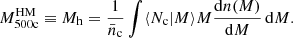
3.2. Splitting the cluster sample

Given our large cluster sample and high signal-to-noise in the stacked cluster lensing measurement we split our sample to investigate the dependence of calibration bias on the cluster mass. As the inferred SZ cluster mass has a large associated uncertainty we split based on the SZ signal-to-noise, since the SZ signal is correlated with the cluster mass. The binning is defined in Table 1 with the corresponding number of clusters in each bin, average SZ inferred mass and average cluster redshift.

We perform both NFW and halo model fits to each SZ signal-to-noise bin following the same procedure as described for the total stack of clusters above. The best fit values are reported in Table 1 for both models. The ESD measurements for each bin with corresponding best fit models are shown in Fig. 5.

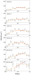Fig. 5. ESD profile (ΔΣ) as a function of radius R, for each sub-sample of clusters. The best fit lines are also plotted shown in red for the single NFW and orange for the halo model.

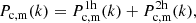
4. Calibration bias: (1 − b_SZ)

To compute the mass bias (1 − b_SZ) we combine estimates of the SZ inferred cluster masses by taking the weighted average. Here clusters are weighted in the same way as in the stacked ESD measurement described in Eq. (15). We estimate the average SZ inferred mass to be $M_{500\mathrm{c}}^{\mathrm{SZ}}=(3.18\pm 0.07)\times {10}^{14}{M}_{\odot }$.

From our halo model estimate of the weak lensing mass, we estimate (1 − b_SZ) = 0.65 ± 0.05. This is consistent with our estimate using a single NFW profile of (1 − b_SZ) = 0.64 ± 0.05. The large deviation of (1 − b_SZ) from unity suggests that clusters are not in hydrostatic equilibrium and that baryon feedback plays an important role; this is consistent with recent results from kinetic SZ and thermal SZ analyses (for example, Koukoufilippas et al. 2020; Ibitoye et al. 2022). This bias, however, cannot be solely attributed to the assumption of hydrostatic equilibrium and is dependent on other assumptions made when estimating M_SZ.

This analysis does not consider the impact of lensing mass bias as investigated in, for example, Becker & Kravtsov (2011) who found a mass bias of 5–10%. For our analysis this level of additional bias in the mass would translate into a shift of up to 1σ in our constraint on (1 − b_SZ). Furthermore Euclid Collaboration (2023) find a similar level of bias of less than 10%, which will be important for future analyses which are more sensitive than this analysis.

In Fig. 4 we show our new estimate together with a compilation of measurements from other data combinations. ACT and Planck cluster mass estimates can be directly compared since they are derived from the same SZ-mass scaling relations and pressure profiles. Our results are consistent with, though generally lower than, analyses of ACT and Planck clusters in a similar mass range using weak galaxy lensing data from Hyper Suprime-Cam (HSC; see Miyatake et al. 2019; Medezinski et al. 2018), CS82 (Battaglia et al. 2016) and CFHTLenS/RCSLenS (Sereno et al. 2017). We also find consistency with the analysis of Planck clusters with CLASH galaxy weak lensing (Penna-Lima et al. 2017) and Planck CMB lensing (Zubeldia & Challinor 2019). Compared to several of the earlier analyses, shown in Fig. 4, we have a slight improvement in constraining power which is due to the larger cluster sample.

Comparing to higher mass Planck cluster analyses, WtG (von der Linden et al. 2014), CCCP (Hoekstra et al. 2015) and its more recent re-analysis CCCP/MENeaCS (Herbonnet et al. 2020), our inferred value for the mass bias is up to 3.8σ lower. Battaglia et al. (2016) demonstrated, however, that adding a correction for Eddington bias (see Sect. 3.1) applied to the SZ mass estimates, would lower the value of (1 − b_SZ) in both the WtG and CCCP analysis (see Fig. 7 in Battaglia et al. 2016). We do apply that correction in this work. In Fig. 4 we show how our result would change if the correction was not applied, with the value we estimate for the mass bias increasing to (1 − b_SZ) = 0.74 ± 0.06, which is a shift of 2σ. It appears that the tension between the value for (1 − b_SZ) found in this work and the recent result from Herbonnet et al. (2020), who found (1 − b_SZ) = 0.84 ± 0.04, can be explained by uncorrected Eddington bias in the latter.

We also find consistency with the mass bias required for Planck primary CMB cosmology to be consistent with the Planck cluster count analysis, which is indicated by the blue band in Fig. 4. To be able to combine all the measurements shown in Fig. 4, we would need to account for covariances between different datasets since some clusters appear in more than one sample and the difference in the ACT and Planck selection functions.

By splitting our sample based on SZ detection signal-to-noise, a quantity correlated with the cluster mass, we investigate whether the bias is mass dependent. The results are reported in Table 1 and shown in Fig. 6. We fit a straight line to M_SZ against (1 − b_SZ), considering two cases: the first just fitting for the y-intercept (no mass dependence) and the second fitting for both the gradient and the y-intercept. We find no evidence for any dependence on mass; with a best fit gradient of 0 ± 0.1. We find that repeating the fit with a gradient of zero still produces an excellent fit, a p-value of 0.9, and only improves the p-value at the sub-percent level when including a mass dependence. Similar results are obtained using the best fit mass estimates from the NFW model. To confirm that this result is not driven by the highest SZ signal-to-noise bin, we perform both fits again excluding this bin and find the same result. This is consistent previous results, which also found no evidence for redshift dependence of the calibration bias (Herbonnet et al. 2020).

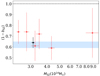Fig. 6. Estimated (1 − bSZ) bias parameter from the total cluster stack shown in black, and in red for six individual SZ signal-to-noise bins. These values are reported in Table 1. The blue band indicates the prediction from Planck primary CMB measurements if the ΛCDM model is correct (Planck Collaboration VI 2020), given the SZ clusters observed by Planck.

5. Conclusions

We have estimated the masses of a new sample of galaxy clusters detected using the Atacama Cosmology Telescope. Stacking the signal from 157 high SZ signal-to-noise clusters, we detect the weak lensing signal at 25σ significance. We estimate the stacked mass to be $M_{500\mathrm{c}}^{\mathrm{WL}}=(4.9\pm 0.4)\times {10}^{14}{M}_{\odot }$, using an analytical halo model formalism which accounts for the ACT SZ cluster selection. By comparing this gravitational lensing estimate of mass to the mass inferred from the SZ signal itself, we provide a new estimate of the calibration of the SZ Compton–y parameter mass scaling relation.

When modelling the cluster lensing signal we adopt two methods, a simpler NFW and a full halo model. The NFW method only models the central halo term and we therefore limit the scales used for this fit to avoid mis-centring at small scales and large-scale structure at scales greater than 5 Mpc. The halo model method assumes an NFW profile for the central halo, however it also accounts for line-of-sight lensing, the ACT selection function and mis-centring. Both mass estimates are consistent within 1σ of each other and have comparable constraining power, which may be initially surprising. This shows that even though we are able to include more data at large and small scales in the halo model fit, the uncertainty on centroiding and the large-scale structure means these extra scales do not help to constrain the mass. The comparable constraining power of these two methods reinforces that our scale cuts for the NFW model fit are correctly defined.

We find our estimate of the mass calibration bias to be consistent, given the statistical uncertainty, with estimates made using other contemporary weak lensing surveys including HSC. This measurement does not indicate a departure from the predicted value of the mass bias from Planck primary CMB measurements if the ΛCDM model is correct (Planck Collaboration VI 2020), given the SZ clusters observed by Planck. Additionally, we find no tension with estimates of the mass bias from a higher mass sample if we do not account for Eddington bias, as first demonstrated in Battaglia et al. (2016).

From splitting our sample based on SZ detection signal-to-noise, which is correlated with the cluster mass, we investigated if the bias has a dependence on mass. Within the statistical uncertainty of our measurements we found no evidence of any dependence on mass which is consistent with the results presented in Herbonnet et al. (2020).

Acknowledgments

The figures in this work were created with matplotlib (Hunter 2007) making use of the numpy (Harris et al. 2020), scipy (Virtanen et al. 2020) and astropy (Astropy Collaboration 2022) software packages. We thank our anonymous referee for their positive feedback and useful comments. N.R. acknowledges support from UK Science and Technology Facilities Council (STFC) under grant ST/V000594/1. C.S. acknowledges support from the Agencia Nacional de Investigación y Desarrollo (ANID) through FONDECYT grant no. 11191125 and BASAL project FB210003. M.B. is supported by the Polish National Science Center through grants no. 2020/38/E/ST9/00395, 2018/30/E/ST9/00698, 2018/31/G/ST9/03388 and 2020/39/B/ST9/03494, and by the Polish Ministry of Science and Higher Education through grant DIR/WK/2018/12. B.G. acknowledges the support of the Royal Society through an Enhancement Award (RGF/EA/181006) and the Royal Society of Edinburgh for support through the Saltire Early Career Fellowship (ref. number 1914). C.H. acknowledges support from the European Research Council under grant number 647112, from the Max Planck Society and the Alexander von Humboldt Foundation in the framework of the Max Planck-Humboldt Research Award endowed by the Federal Ministry of Education and Research, and the UK Science and Technology Facilities Council (STFC) under grant ST/V000594/1. H.H. is supported by a Heisenberg grant of the Deutsche Forschungsgemeinschaft (Hi 1495/5-1) as well as an ERC Consolidator Grant (No. 770935). H.H. acknowledges support from Vici grant 639.043.512, financed by the Netherlands Organisation for Scientific Research (NWO). M.H. acknowledges support from the National Research Foundation of South Africa (grant no. 137975). J.P.H. gratefully acknowledges support from the estate of George A. and Margaret M. Downsbrough. H.Y.S. acknowledges the support from CMS-CSST-2021-A01 and CMS-CSST-2021-B01, NSFC of China under grant 11973070, and Key Research Program of Frontier Sciences, CAS, Grant No. ZDBS-LY-7013. T.T. acknowledges funding from the Swiss National Science Foundation under the Ambizione project PZ00P2_193352. A.H.W. is supported by an European Research Council Consolidator Grant (No. 770935). Support for ACT was through the US National Science Foundation through awards AST-0408698, AST-0965625, and AST-1440226 for the ACT project, as well as awards PHY-0355328, PHY-0855887 and PHY-1214379. Funding was also provided by Princeton University, the University of Pennsylvania, and a Canada Foundation for Innovation (CFI) award to UBC. ACT operated in the Parque Astronómico Atacama in northern Chile under the auspices of the Agencia Nacional de Investigación y Desarrollo (ANID). The development of multichroic detectors and lenses was supported by NASA grants NNX13AE56G and NNX14AB58G. Detector research at NIST was supported by the NIST Innovations in Measurement Science program. Author contributions: All authors contributed to the development and writing of this paper. The authorship list is given in two groups: the lead authors (NCR & CS) followed by an alphabetical group of those who made significant contributions to the scientific analysis and/or the ACT or KiDS surveys.

References

Appendix A: Mis-centring of clusters

The mis-centring of clusters has been reported as one of the largest biases when estimating the cluster mass from weak gravitational lensing (e.g. Sommer et al. 2022; Ford et al. 2015). If the true cluster centre has not been identified then the amplitude of the ESD will be reduced at small radii, corresponding to a lower mass estimate for the cluster.

We consider two different cluster centre definitions: the peak of the SZ emission and the Brightest Cluster Galaxy (BCG), which has been shown to be the best tracer of the cluster centre (George et al. 2012). The SZ centre is not expected to trace the centre precisely since it is limited by the size of the beam which is 1.4 arcmin for ACT; this corresponds to R = 0.09 Mpc for z_l = 0.1 and R = 0.62 Mpc for z_l = 0.9. We also anticipate that most clusters are not relaxed and therefore the gas is not expected to trace the centre of the dark matter halo.

We find the BCG for each cluster by selecting KiDS galaxies found inside a cylinder, centred on the SZ peak, with a length |z_B − z_l| = 2 × 0.04(1 + z_l), where z_B is the photometric redshift of a KiDS galaxy, and a diameter 2 × 1.4 arcmin. The length of the cylinder is defined to be twice the length of the uncertainty on the photometric redshift of the KiDS galaxies, and the diameter is defined based on the size of the ACT beam. From these galaxies the brightest one is chosen. We then confirm the BCG locations by visual inspection, using public imaging from KiDS, the Dark Energy Camera Legacy Survey and Hyper Suprime-Cam. We note that for some clusters (for example one of the most massive clusters in our sample, Abell 2744/ACT-CL J0014.3−3022) that are undergoing merging and therefore far from being in a virialised state, it is difficult assign an appropriate centre.

Measuring the ESD around both these centre candidates, we find at small radii the ESD measured around the BCG has a higher amplitude than measured around the SZ centre, which agrees with our expectation – this is shown in Fig. A.1. The ratio between the BCG and SZ centred signal when averaged R > 0.5Mpc is unity, compared to the same ratio having a value of ∼5 when averaged R < 0.5Mpc.

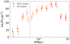Fig. A.1. Tests of mis-centring: comparison of the ESD measured around the peak in the SZ emission and the BCG. The ratio between the BCG and SZ centred signal averaged R > 0.5 is unity.

All Tables

All Figures

Fig. 1. KiDS North and South survey areas are shown in light grey in the upper and lower panels, respectively. The positions of ACT clusters used in this analysis are indicated by each circle. The colour of the circles corresponds to cluster redshift, with yellow indicating high redshift and black indicating low redshift. The size of each circle scales with the SZ signal-to-noise, which is correlated with the cluster mass when the noise is the same everywhere, such that larger circles represent clusters with a greater SZ signal-to-noise than smaller circles.

In the text

Fig. 2. Upper: normalised SZ signal-to-noise distribution of the ACT clusters found in the KiDS-1000 region. Middle: normalised redshift distribution of these clusters. Lower: normalised SZ-derived mass distribution of these clusters, estimated from the SZ observable Compton–y values. The blue shaded region corresponds to clusters selected to have an SZ signal-to-noise greater than 5 and in the redshift range 0.1–0.9 across the full ACT footprint. The orange line corresponds to the selection of 157 clusters used in this analysis that lie within the KiDS footprint.

In the text

Fig. 3. ESD profile (ΔΣ) multiplied by the radius R as a function of radius R for the complete stack of 157 SZ-detected clusters. The signal is detected at 25σ significance. The best-fitting model is shown using a single NFW, shown in red, and the halo model, shown in orange. A limited range of scales is used for the NFW model to avoid the impact of mis-centring at small scales and the contribution from large-scale structure at scales greater than 5 Mpc. Both models give good fits to the data.

In the text

Fig. 4. Estimated (1 − bSZ) bias parameter from this analysis (ACT SZ-detected clusters calibrated with KiDS weak lensing), compared to other recent results. Shown on this figure at the lower mass range, the analyses of ACT and Planck clusters using HSC (Miyatake et al. 2019; Medezinski et al. 2018), ACT/CS82 (Battaglia et al. 2016), CLASH (Penna-Lima et al. 2017), PSZ2LenS (Sereno et al. 2017), WtG (von der Linden et al. 2014), CCCP (Hoekstra et al. 2015) which has recently been updated to CCCP and MENeaCS (Herbonnet et al. 2020) and Planck clusters with Planck CMB lensing (Zubeldia & Challinor 2019) analyses. The blue band indicates the prediction from Planck primary CMB measurements if the ΛCDM model is correct (Planck Collaboration VI 2020), given the SZ clusters observed by Planck. This value is computed using a Planck Collaboration VI (2020) primary CMB best fit cosmology, however using the cosmology derived from ACT DR6 lensing, Madhavacheril et al. (2023), would give the same result.

In the text

	Fig. 5. ESD profile (ΔΣ) as a function of radius R, for each sub-sample of clusters. The best fit lines are also plotted shown in red for the single NFW and orange for the halo model.
In the text

	Fig. 6. Estimated (1 − bSZ) bias parameter from the total cluster stack shown in black, and in red for six individual SZ signal-to-noise bins. These values are reported in Table 1. The blue band indicates the prediction from Planck primary CMB measurements if the ΛCDM model is correct (Planck Collaboration VI 2020), given the SZ clusters observed by Planck.
In the text

	Fig. A.1. Tests of mis-centring: comparison of the ESD measured around the peak in the SZ emission and the BCG. The ratio between the BCG and SZ centred signal averaged R > 0.5 is unity.
In the text

References

- Allen, S. W., Evrard, A. E., & Mantz, A. B. 2011, ARA&A, 49, 409 [Google Scholar]
- Applegate, D. E., von der Linden, A., Kelly, P. L., et al. 2014, MNRAS, 439, 48 [Google Scholar]
- Arnaud, M., Pratt, G. W., Piffaretti, R., et al. 2010, A&A, 517, A92 [CrossRef] [EDP Sciences] [Google Scholar]
- Asgari, M., Lin, C.-A., Joachimi, B., et al. 2021, A&A, 645, A104 [NASA ADS] [CrossRef] [EDP Sciences] [Google Scholar]
- Astropy Collaboration (Price-Whelan, A. M., et al.) 2022, ApJ, 935, 167 [NASA ADS] [CrossRef] [Google Scholar]
- Bartelmann, M., & Schneider, P. 2001, Phys. Rep., 340, 291 [Google Scholar]
- Battaglia, N., Leauthaud, A., Miyatake, H., et al. 2016, JCAP, 2016, 013 [NASA ADS] [CrossRef] [Google Scholar]
- Becker, M. R., & Kravtsov, A. V. 2011, ApJ, 740, 25 [NASA ADS] [CrossRef] [Google Scholar]
- Benítez, N. 2000, ApJ, 536, 571 [Google Scholar]
- Birkinshaw, M., Gull, S. F., & Hardebeck, H. 1984, Nature, 309, 34 [NASA ADS] [CrossRef] [Google Scholar]
- Bocquet, S., Dietrich, J. P., Schrabback, T., et al. 2019, ApJ, 878, 55 [Google Scholar]
- Bode, P., Ostriker, J. P., Cen, R., & Trac, H. 2012, arXiv e-prints [arXiv:1204.1762] [Google Scholar]
- Böhringer, H., Schuecker, P., Guzzo, L., et al. 2004, A&A, 425, 367 [NASA ADS] [CrossRef] [EDP Sciences] [Google Scholar]
- Chisari, N. E., Alonso, D., Krause, E., et al. 2019, ApJS, 242, 2 [Google Scholar]
- Cooray, A., & Sheth, R. 2002, Phys. Rep., 372, 1 [Google Scholar]
- Cromer, D., Battaglia, N., Miyatake, H., & Simet, M. 2022, JCAP, 2022, 034 [CrossRef] [Google Scholar]
- de Jong, J. T. A., Verdoes Kleijn, G. A., Boxhoorn, D. R., et al. 2015, A&A, 582, A62 [NASA ADS] [CrossRef] [EDP Sciences] [Google Scholar]
- Debackere, S. N. B., Schaye, J., & Hoekstra, H. 2021, MNRAS, 505, 593 [NASA ADS] [CrossRef] [Google Scholar]
- Dietrich, J. P., Bocquet, S., Schrabback, T., et al. 2019, MNRAS, 483, 2871 [Google Scholar]
- Ebeling, H., Edge, A. C., Bohringer, H., et al. 1998, MNRAS, 301, 881 [Google Scholar]
- Edge, A., Sutherland, W., Kuijken, K., et al. 2013, Messenger, 154, 32 [Google Scholar]
- Euclid Collaboration (Giocoli, C., et al.) 2023, A&A, in press, https://doi.org/10.1051/0004-6361/202346058 [Google Scholar]
- Ford, J., Van Waerbeke, L., Milkeraitis, M., et al. 2015, MNRAS, 447, 1304 [CrossRef] [Google Scholar]
- Foreman-Mackey, D., Hogg, D. W., Lang, D., & Goodman, J. 2013, PASP, 125, 306 [Google Scholar]
- George, M. R., Leauthaud, A., Bundy, K., et al. 2012, ApJ, 757, 2 [NASA ADS] [CrossRef] [Google Scholar]
- Giblin, B., Heymans, C., Asgari, M., et al. 2021, A&A, 645, A105 [NASA ADS] [CrossRef] [EDP Sciences] [Google Scholar]
- Gladders, M. D., & Yee, H. K. C. 2005, ApJS, 157, 1 [NASA ADS] [CrossRef] [Google Scholar]
- Harris, C. R., Millman, K. J., van der Walt, S. J., et al. 2020, Nature, 585, 357 [NASA ADS] [CrossRef] [Google Scholar]
- Hasselfield, M., Hilton, M., Marriage, T. A., et al. 2013, JCAP, 2013, 008 [Google Scholar]
- Henson, M. A., Barnes, D. J., Kay, S. T., McCarthy, I. G., & Schaye, J. 2017, MNRAS, 465, 3361 [NASA ADS] [CrossRef] [Google Scholar]
- Herbonnet, R., Sifón, C., Hoekstra, H., et al. 2020, MNRAS, 497, 4684 [NASA ADS] [CrossRef] [Google Scholar]
- Heymans, C., Tröster, T., Asgari, M., et al. 2021, A&A, 646, A140 [NASA ADS] [CrossRef] [EDP Sciences] [Google Scholar]
- High, F. W., Hoekstra, H., Leethochawalit, N., et al. 2012, ApJ, 758, 68 [NASA ADS] [CrossRef] [Google Scholar]
- Hildebrandt, H., van den Busch, J. L., Wright, A. H., et al. 2021, A&A, 647, A124 [EDP Sciences] [Google Scholar]
- Hilton, M., Sifón, C., Naess, S., et al. 2021, ApJS, 253, 3 [Google Scholar]
- Hoekstra, H. 2001, A&A, 370, 743 [NASA ADS] [CrossRef] [EDP Sciences] [Google Scholar]
- Hoekstra, H., Franx, M., & Kuijken, K. 2000, ApJ, 532, 88 [Google Scholar]
- Hoekstra, H., Bartelmann, M., Dahle, H., et al. 2013, Space Sci. Rev., 177, 75 [NASA ADS] [CrossRef] [Google Scholar]
- Hoekstra, H., Herbonnet, R., Muzzin, A., et al. 2015, MNRAS, 449, 685 [NASA ADS] [CrossRef] [Google Scholar]
- Hunter, J. D. 2007, Comput. Sci. Eng., 9, 90 [NASA ADS] [CrossRef] [Google Scholar]
- Ibitoye, A., Tramonte, D., Ma, Y.-Z., & Dai, W.-M. 2022, ApJ, 935, 18 [NASA ADS] [CrossRef] [Google Scholar]
- Itoh, N., Kohyama, Y., & Nozawa, S. 1998, ApJ, 502, 7 [Google Scholar]
- Jee, M. J., Hughes, J. P., Menanteau, F., et al. 2014, ApJ, 785, 20 [NASA ADS] [CrossRef] [Google Scholar]
- Kannawadi, A., Hoekstra, H., Miller, L., et al. 2019, A&A, 624, A92 [NASA ADS] [CrossRef] [EDP Sciences] [Google Scholar]
- Koukoufilippas, N., Alonso, D., Bilicki, M., & Peacock, J. A. 2020, MNRAS, 491, 5464 [Google Scholar]
- Kuijken, K., Heymans, C., Dvornik, A., et al. 2019, A&A, 625, A2 [NASA ADS] [CrossRef] [EDP Sciences] [Google Scholar]
- Madhavacheril, M. S., Qu, F. J., Sherwin, B. D., et al. 2023, ApJ, submitted [arXiv:2304.05203] [Google Scholar]
- Mandelbaum, R., Hirata, C. M., Ishak, M., Seljak, U., & Brinkmann, J. 2006, MNRAS, 367, 611 [CrossRef] [Google Scholar]
- McInnes, R. N., Menanteau, F., Heavens, A. F., et al. 2009, MNRAS, 399, L84 [NASA ADS] [Google Scholar]
- Medezinski, E., Battaglia, N., Umetsu, K., et al. 2018, PASJ, 70, S28 [NASA ADS] [Google Scholar]
- Miller, L., Heymans, C., Kitching, T. D., et al. 2013, MNRAS, 429, 2858 [Google Scholar]
- Miyatake, H., Nishizawa, A. J., Takada, M., et al. 2013, MNRAS, 429, 3627 [NASA ADS] [CrossRef] [Google Scholar]
- Miyatake, H., Battaglia, N., Hilton, M., et al. 2019, ApJ, 875, 63 [Google Scholar]
- Naess, S., Aiola, S., Austermann, J. E., et al. 2020, JCAP, 2020, 046 [Google Scholar]
- Nagai, D. 2006, ApJ, 650, 538 [Google Scholar]
- Navarro, J. F., Frenk, C. S., & White, S. D. M. 1997, ApJ, 490, 493 [Google Scholar]
- Peacock, J. A., & Smith, R. E. 2000, MNRAS, 318, 1144 [Google Scholar]
- Penna-Lima, M., Bartlett, J. G., Rozo, E., et al. 2017, A&A, 604, A89 [NASA ADS] [CrossRef] [EDP Sciences] [Google Scholar]
- Planck Collaboration XXIV. 2016, A&A, 594, A24 [NASA ADS] [CrossRef] [EDP Sciences] [Google Scholar]
- Planck Collaboration VI. 2020, A&A, 641, A6 [NASA ADS] [CrossRef] [EDP Sciences] [Google Scholar]
- Remazeilles, M., Bolliet, B., Rotti, A., & Chluba, J. 2019, MNRAS, 483, 3459 [Google Scholar]
- Rykoff, E. S., Rozo, E., Hollowood, D., et al. 2016, ApJS, 224, 1 [NASA ADS] [CrossRef] [Google Scholar]
- Schrabback, T., Applegate, D., Dietrich, J. P., et al. 2018, MNRAS, 474, 2635 [Google Scholar]
- Seitz, C., & Schneider, P. 1997, A&A, 318, 687 [NASA ADS] [Google Scholar]
- Seljak, U. 2000, MNRAS, 318, 203 [Google Scholar]
- Sereno, M., Covone, G., Izzo, L., et al. 2017, MNRAS, 472, 1946 [Google Scholar]
- Sheldon, E. S., Johnston, D. E., Frieman, J. A., et al. 2004, AJ, 127, 2544 [Google Scholar]
- Sifón, C., Menanteau, F., Hasselfield, M., et al. 2013, ApJ, 772, 25 [CrossRef] [Google Scholar]
- Singh, S., Mandelbaum, R., Seljak, U., Slosar, A., & Vazquez Gonzalez, J. 2017, MNRAS, 471, 3827 [Google Scholar]
- Sommer, M. W., Schrabback, T., Applegate, D. E., et al. 2022, MNRAS, 509, 1127 [Google Scholar]
- Stern, C., Dietrich, J. P., Bocquet, S., et al. 2019, MNRAS, 485, 69 [NASA ADS] [CrossRef] [Google Scholar]
- Sunyaev, R. A., & Zel’dovich, Y. B. 1972, Comm. Astrophys. Space Phys., 4, 173 [Google Scholar]
- Tinker, J. L., Robertson, B. E., Kravtsov, A. V., et al. 2010, ApJ, 724, 878 [NASA ADS] [CrossRef] [Google Scholar]
- Vikhlinin, A., Burenin, R. A., Ebeling, H., et al. 2009, ApJ, 692, 1033 [Google Scholar]
- Virtanen, P., Gommers, R., Oliphant, T. E., et al. 2020, Nat. Methods, 17, 261 [Google Scholar]
- von der Linden, A., Mantz, A., Allen, S. W., et al. 2014, MNRAS, 443, 1973 [NASA ADS] [CrossRef] [Google Scholar]
- Wright, C. O., & Brainerd, T. G. 2000, ApJ, 534, 34 [Google Scholar]
- Wright, A. H., Hildebrandt, H., Kuijken, K., et al. 2019, A&A, 632, A34 [NASA ADS] [CrossRef] [EDP Sciences] [Google Scholar]
- Wright, A. H., Hildebrandt, H., van den Busch, J. L., et al. 2020, A&A, 640, L14 [NASA ADS] [CrossRef] [EDP Sciences] [Google Scholar]
- Zel’dovich, Y. B., & Sunyaev, R. A. 1969, Ap&SS, 4, 301 [NASA ADS] [CrossRef] [Google Scholar]
- Zubeldia, Í., & Challinor, A. 2019, MNRAS, 489, 401 [NASA ADS] [CrossRef] [Google Scholar]